CalcI_Derivatives_Apps_Solutions pdf - عبدالرحمن سهيل

CALCULUS I

Solutions to Practice Problems

Applications of Derivatives

Paul Dawkins

Calculus I

http://tutorial.math.lamar.edu/terms.aspx

Table of Contents

Preface ............................................................................................................................................ 1

Applications of Derivatives ........................................................................................................... 1

Rates of Change......................................................................................................................................... 2

Critical Points ............................................................................................................................................ 2

Minimum and Maximum Values .............................................................................................................16

Finding Absolute Extrema ......................................................................................................................27

The Shape of a Graph, Part I....................................................................................................................43

The Shape of a Graph, Part II ..................................................................................................................66

The Mean Value Theorem .......................................................................................................................94

Optimization ............................................................................................................................................99

More Optimization Problems ...............................................................................................................112

Indeterminate Forms and L’Hospital’s Rule ........................................................................................127

Linear Approximations .........................................................................................................................141

Differentials ...........................................................................................................................................145

Newton’s Method ...................................................................................................................................148

Business Applications ...........................................................................................................................159

Preface

Here are the solutions to the practice problems for my Calculus I notes.  Some solutions will have
more or less detail than other solutions. The level of detail in each solution will depend up on
several issues. If the section is a review section, this mostly applies to problems in the first
chapter, there will probably not be as much detail to the solutions given that the problems really
should be review. As the difficulty level of the problems increases less detail will go into the
basics of the solution under the assumption that if you’ve reached the level of working the harder
problems then you will probably already understand the basics fairly well and won’t need all the
explanation.

This document was written with presentation on the web in mind. On the web most solutions are
broken down into steps and many of the steps have hints. Each hint on the web is given as a
popup however in this document they are listed prior to each step. Also, on the web each step can
be viewed individually by clicking on links while in this document they are all showing. Also,
there are liable to be some formatting parts in this document intended for help in generating the
web pages that haven’t been removed here.  These issues may make the solutions a little difficult
to follow at times, but they should still be readable.

Applications of Derivatives

Calculus I

http://tutorial.math.lamar.edu/terms.aspx

Rates of Change

As noted in the text for this section the purpose of this section is only to remind you of certain
types of applications that were discussed in the previous chapter. As such there aren’t any
problems written for this section. Instead here is a list of links (note that these will only be active
links in the web version and not the pdf version) to problems from the relevant sections from the
previous chapter.

Each of the following sections has a selection of increasing/decreasing problems towards the
bottom of the problem set.

Differentiation Formulas

Product & Quotient Rules

Derivatives of Trig Functions

Derivatives of Exponential and Logarithm Functions

Chain Rule

Related Rates problems are in the

Related Rates

section.

Critical Points

1. Determine the critical points of

( )

f x

−

Step 1
We’ll need the first derivative to get the answer to this problem so let’s get that.

( )

(

)(

)

162

7 4

′

−

Factoring the derivative as much as possible will help with the next step.

Step 2
Recall that critical points are simply where the derivative is zero and/or doesn’t exist. In this case
the derivative is just a polynomial and we know that exists everywhere and so we don’t need to
worry about that. So, all we need to do is set the derivative equal to zero and solve for the critical
points.

(

)(

)

1
4

− =

⇒

= −

2. Determine the critical points of

( )

1 80

R t

= +

−

Calculus I

http://tutorial.math.lamar.edu/terms.aspx

Step 1
We’ll need the first derivative to get the answer to this problem so let’s get that.

( )

(

)(

)

240

R t

′

−

= −

−

(

)(

)

−

⇒

= −

3. Determine the critical points of

( )

g w

−

Step 1
We’ll need the first derivative to get the answer to this problem so let’s get that.

( )

g w

′

−

Step 2
Recall that critical points are simply where the derivative is zero and/or doesn’t exist. In this case
the derivative is just a polynomial and we know that exists everywhere and so we don’t need to
worry about that. So, all we need to do is set the derivative equal to zero and solve for the critical
points.

268

−

− =

⇒

As we can see in this case we needed to use the quadratic formula to find the critical points. Not
all quadratics will factor so don’t forget about the quadratic formula!

4. Determine the critical points of

( )

g x

−

Step 1
We’ll need the first derivative to get the answer to this problem so let’s get that.

Calculus I

http://tutorial.math.lamar.edu/terms.aspx

( )

(

)

g x

′

−

(

)

−

⇒

−

From the first term we clearly see that

is a critical point. The second term does not factor

and we we’ll need to use the quadratic formula to solve this equation.

167

± −

Remember that not all quadratics will factor so don’t forget about the quadratic formula!

Step 3
Now, recall that we don’t use complex numbers in this class and so the solutions from the second
term are not critical points. Therefore, the only critical point of this function is,

5. Determine the critical points of

( )

h z

−

Step 1
We’ll need the first derivative to get the answer to this problem so let’s get that.

( )

h z

′

−

Calculus I

http://tutorial.math.lamar.edu/terms.aspx

396

± −

−

+ =

⇒

As we can see in this case we needed to use the quadratic formula to solve the quadratic.
Remember that not all quadratics will factor so don’t forget about the quadratic formula!

Step 3
Now, recall that we don’t use complex numbers in this class and so the solutions are not critical
points. Therefore, there are no critical points for this function.

Do not get excited about there being no critical points for a function. There is no rule that says
that every function has to have critical points!

6. Determine the critical points of

( ) (

)

(

)

2 8

Q x

−

Step 1
We’ll need the first derivative to get the answer to this problem so let’s get that.

( ) (

) ( )

(

)

(

) ( )

(

)

( )

(

)

(

)

(

)

(

)

(

)

(

)

(

)

(

)

4 2 8

2 8

2 2 8

2 8

2 2 8

144

4 2 8

Q x

′

−

+ −

−





−

− +

−













−

= −

−









Factoring the derivative as much as possible will help with the next step. For this problem
(unlike some of the previous problems) this extra factoring is all but required to make this easier
to finish.

Step 2
Recall that critical points are simply where the derivative is zero and/or doesn’t exist. In this case
the derivative is just a polynomial, (admittedly a somewhat messy polynomial) and we know that
exists everywhere and so we don’t need to worry about that. So, all we need to do is set the
derivative equal to zero and solve for the critical points.

(

)

(

)

4 2 8





−





From this we get the following three equations that we need to solve.

Calculus I

http://tutorial.math.lamar.edu/terms.aspx

(

)

(

)

2 8

−

For the first two equations all we really need to do is set the quantity inside the parenthesis to
zero (the exponent on the parenthesis won’t affect the solution) and the third requires the
quadratic formula.

1
4

2 8

−

⇒

− =

⇒

= ±

( )(

)

( )

4 20

5769

2 20

−

⇒

So, we get the 5 critical points boxed in above.

7. Determine the critical points of

( )

f z

+ +

Step 1
We’ll need the first derivative to get the answer to this problem so let’s get that.

( )

(

)

(

)(

)

(

)

(

)

(

)

(

)

1 2

4 4

+ + − +

−

′

+ +

The “-2” was factored out of the numerator only to make it a little nicer for the next step and
doesn’t really need to be done.

Step 2
Recall that critical points are simply where the derivative is zero and/or doesn’t exist. In this case
the derivative is a rational expression. Therefore we know that the derivative will be zero if the
numerator is zero (and the denominator is also not zero for the same values of course). We also
know that the derivative won’t exist if we get division by zero.

So, all we need to do is set the numerator and denominator equal to zero and solve. Note as well
that the “-2” we factored out of the numerator will not affect where it is zero and so can be
ignored. Likewise, the exponent on the whole denominator will not affect where it is zero and so
can also be ignored. This means we need to solve the following two equations.

Calculus I

http://tutorial.math.lamar.edu/terms.aspx

4 3 2

− ±

− =

⇒

= − ±

− ± −

− ±

+ + =

⇒

As we can see in this case we needed to use the quadratic formula both of the quadratic equations.
Remember that not all quadratics will factor so don’t forget about the quadratic formula!

Step 3
Now, recall that we don’t use complex numbers in this class and so the solutions from where the
denominator is zero (i.e. the derivative doesn’t exist) won’t be critical points. Therefore, the only
critical points of this function are,

4 3 2

= − ±

8. Determine the critical points of

( )

R x

−

Step 1
We’ll need the first derivative to get the answer to this problem so let’s get that.

( )

(

)

(

)(

)

(

)

(

)

R x

−

− −

−

′

−

Step 2
Recall that critical points are simply where the derivative is zero and/or doesn’t exist. In this case
the derivative is a rational expression. Therefore we know that the derivative will be zero if the
numerator is zero (and the denominator is also not zero for the same values of course). We also
know that the derivative won’t exist if we get division by zero.

So, all we need to do is set the numerator and denominator equal to zero and solve. Note that the
exponent on the whole denominator will not affect where it is zero and so can be ignored. This
means we need to solve the following two equations.

1 2 3

± −

−

⇒

= ±

(

)(

)

5, 3

−

− =

⇒

= −

Calculus I

http://tutorial.math.lamar.edu/terms.aspx

As we can see in this case we needed to use the quadratic formula on the first quadratic equation.
Remember that not all quadratics will factor so don’t forget about the quadratic formula!

Step 3
Now, recall that we don’t use complex numbers in this class and so the solutions from where the
numerator is zero won’t be critical points.

Also recall that a point will only be a critical point if the function (not the derivative, but the
original function) exists at the point. For this problem we found two values where the derivative
doesn’t exist, however the function also doesn’t exist at these points and so neither of these will
be critical points either.

Therefore, this function has no critical points. Do not get excited about this when it happens.
Not all functions will have critical points!

9. Determine the critical points of

( )

r y

−

Step 1
We’ll need the first derivative to get the answer to this problem so let’s get that.

( ) (

)

(

)

(

)

r y

−

′

−

We took the term with the negative exponent to the denominator for the discussion in the next
step.  While it doesn’t really need to be done this will make sure that there are no inadvertent
mistakes down the road.

Step 2
Recall that critical points are simply where the derivative is zero and/or doesn’t exist. In this case
the derivative is a rational expression. Therefore we know that the derivative will be zero if the
numerator is zero (and the denominator is also not zero for the same values of course). We also
know that the derivative won’t exist if we get division by zero.

So, all we need to do is set the numerator and denominator equal to zero and solve. Note that the
exponent on the whole denominator will not affect where it is zero and so can be ignored.  This
means we need to solve the following two equations.

− =

⇒

(

)

0, 6

y y

−

⇒

Step 3

Calculus I

http://tutorial.math.lamar.edu/terms.aspx

Note as well that the reason for moving the term to the denominator as we did in the first step is
to make it clear that the last two critical points are critical points because the derivative does not
exist at those points and not because the derivative is zero at those points. Also note that they are
critical points because the function does exist at these points.

Therefore, along with the first critical point (where the derivative is zero), we get the following
critical points for this function.

0, 3, 6

10. Determine the critical points of

( )

(

)

h t





− −

− +





Step 1
We’ll need the first derivative to get the answer to this problem so let’s get that.

( )

(

)

( )

(

)

(

)(

)

(

)

(

)(

)

(

)

(

)

h t

−

′













− +

− −

−

− +

−

















− +





− + − −

−

− +

After differentiating we moved the term with the negative exponent to the denominator and then
combined everything into a single term. This will help with the next step considerably.

Step 2
Recall that critical points are simply where the derivative is zero and/or doesn’t exist.

Because we moved the term with the negative exponent to the denominator and then combined
everything into a single term we now have written the derivative as a rational expression.
Therefore we know that the derivative will be zero if the numerator is zero (and the denominator
is also not zero for the same values of course).  We also know that the derivative won’t exist if we
get division by zero.

So, all we need to do is set the numerator and denominator equal to zero and solve. Note that the
exponent on the whole denominator will not affect where it is zero and so can be ignored. This
means we need to solve the following two equations.

544

19 2 34

−

⇒

Calculus I

http://tutorial.math.lamar.edu/terms.aspx

(

)(

)

1, 7

− + = −

− =

⇒

Step 3
Note that because we combined all the terms in the derivative into a single term it was much
easier to determine the critical points for this function. If we had not combined the terms the
solving work would have been more complicated, although not impossible.

Doing this also makes it clear that the last two critical points are critical points because the
derivative does not exist at those points and not because the derivative is zero at those points.
Also note that they are critical points because the function does exist at these points.

Therefore, along with the first two critical points (where the derivative is zero), we get the
following critical points for this function.

2 34

1, 7,

11. Determine the critical points of

( )

4 cos

s z

−

Step 1
We’ll need the first derivative to get the answer to this problem so let’s get that.

( )

4 sin

s z

′

= −

−

Step 2
Recall that critical points are simply where the derivative is zero and/or doesn’t exist.

This derivative exists everywhere and so we don’t need to worry about that. Therefore all we
need to do is determine where the derivative is zero. So, all we need to do is solve the equation,

( )

4 sin

sin

0.2527

−

− =

→

= −

→

−

= −

This is the answer we got from a calculator and we could use this or we could use the equivalent

positive angle :

0.2527

6.0305

−

. Either can be used, but we’ll use the positive one for

this problem.

Now, a quick look at a unit circle gives us a second solution of

0.2527

3.3943

Finally all possible solutions to this equation, and hence, all the critical points of the original
function are,

Calculus I

http://tutorial.math.lamar.edu/terms.aspx

6.0305 2

0, 1, 2, ,

3.3943 2

π
π

= ± ± ±



If you don’t remember how to solve trig equations you should go back and review those sections
in the Review Chapter of the notes.

12. Determine the critical points of

( )

sin

f y

Step 1
We’ll need the first derivative to get the answer to this problem so let’s get that.

( )

cos

′

( )

cos

2.3005

−

+ =

→

= −

→

−

This is the answer we got from a calculator and a quick look at a unit circle gives us a second
solution of either -2.3005 or if you want the positive equivalent we could use

2.3005

3.9827

−

. For this problem we’ll use the positive one, although the negative one

could just as easily be used if you wanted to.

All possible solutions to

( )

cos

= −

are then,

2.3005 2

0, 1, 2, ,

3.9827

π
π

= ± ± ±



Finally solving for y gives all the critical points of the function.

6.9015 6

0, 1, 2, ,

11.9481 6

= ± ± ±



If you don’t remember how to solve trig equations you should go back and review those sections
in the Review Chapter of the notes.

Calculus I

http://tutorial.math.lamar.edu/terms.aspx

13. Determine the critical points of

( )

sin

V t

Step 1
We’ll need the first derivative to get the answer to this problem so let’s get that.

( )

( ) ( )

6 sin 3 cos 3

V t

′

( ) ( )

( )

6 sin 3 cos 3

sin 3

cos 3

→

Step 3
So, we now need to solve these two trig equations.

From a quick look at a unit circle we can see that sine is zero at 0 and

and so all solutions to

( )

sin 3

are then,

2
3

0 2

0, 1, 2, ,

= +

→

= ± ± ±

= +



Another look at a unit circle and we can see that cosine is zero at

and

and so all solutions

( )

cos 3

are then,

0, 1, 2, ,

= +

→

= ± ± ±

= +



Therefore, critical points of the function are,

0, 1, 2, ,

n t

= +

= ± ± ± 

If you don’t remember how to solve trig equations you should go back and review those sections
in the Review Chapter of the notes.

14. Determine the critical points of

( )

9 2

f x

−

Calculus I

http://tutorial.math.lamar.edu/terms.aspx

Step 1
We’ll need the first derivative to get the answer to this problem so let’s get that.

( )

(

)

9 2

1 2

−

′

−

We did some quick factoring to help with the next step and while it doesn’t technically need to be
done it will significantly reduce the amount work required in the next step.

Step 2
Recall that critical points are simply where the derivative is zero and/or doesn’t exist.

This derivative exists everywhere and so we don’t need to worry about that.  Therefore all we
need to do is determine where the derivative is zero.

Notice as well that because we know that exponential functions are never zero and so the
derivative will only be zero if,

1
2

1 2

−

→

So, we have a single critical point,

1
2

, for this function.

15. Determine the critical points of

( )

g w

−

= e

Step 1
We’ll need the first derivative to get the answer to this problem so let’s get that.

( )

(

)

(

)(

)

g w

−

′

−

We did some quick factoring to help with the next step.

Step 2
Recall that critical points are simply where the derivative is zero and/or doesn’t exist.

This derivative exists everywhere and so we don’t need to worry about that.  Therefore all we
need to do is determine where the derivative is zero.

Notice as well that because we know that exponential functions are never zero and so the
derivative will only be zero if,

Calculus I

http://tutorial.math.lamar.edu/terms.aspx

(

)(

)

7
3

−

+ =

→

−

So, we have a two critical points,

7
3

and

= −

for this function.

16. Determine the critical points of

( )

(

)

R x

Step 1
We’ll need the first derivative to get the answer to this problem so let’s get that.

( )

R x

′

Step 2
Recall that critical points are simply where the derivative is zero and/or doesn’t exist. In this case
the derivative is a rational expression.

So, we know that the derivative will be zero if the numerator is zero (and the denominator is also
not zero for the same values of course).

We also know that the derivative won’t exist if we get division by zero. However, in this case
note that the denominator is also the polynomial that is inside the logarithm and so any values of
x for which the denominator is zero will not be in the domain of the original function (i.e. the

function,

( )

R x

, won’t exist at those values of x because we can’t take the logarithm of zero).

Therefore, these points will not be critical points and we don’t need to bother determining where
the derivative will be zero.

So, setting the numerator equal to zero gives,

+ =

⇒

= −

Step 3

As a final step we really should check that

( )

−

exists since there is always a chance that it

won’t since we are dealing with a logarithm. It does exist (

( )

ln 10

− =

) and so the only

critical point for this function is,

= −

Calculus I

http://tutorial.math.lamar.edu/terms.aspx

17. Determine the critical points of

( )

(

)

7 ln 8

A t

= −

Step 1
We’ll need the first derivative to get the answer to this problem so let’s get that.

( )

3 7

A t

−





′

= −









We did quite a bit of simplification of the derivative to help with the next step. While not
technically required it will mean the next step will be a fair amount simpler to do.

Step 2
Recall that critical points are simply where the derivative is zero and/or doesn’t exist. In this case
the derivative is a rational expression.

So, we know that the derivative will be zero if the numerator is zero (and the denominator is also
not zero for the same values of course).

We also know that the derivative won’t exist if we get division by zero. However, in this case
note that the denominator is also the polyomial that is inside the logarithm and so any values of t

for which the denominator is zero (i.e.

1
4

= −

since it’s easy to see that point) will not be in the

domain of the original function (i.e. the function,

( )

1
4

−

, won’t exist because we can’t take the

logarithm of zero). Therefore, this point will not be a critical point.

So, setting the numerator equal to zero gives,

−

⇒

Step 3

As a final step we really should check that

( )

exists since there is always a chance that it

won’t since we are dealing with a logarithm. It does exist (

( )

7 ln

= −

) and so the

only critical point for this function is,

Calculus I

http://tutorial.math.lamar.edu/terms.aspx

Minimum and Maximum Values

1. Below is the graph of some function,

( )

f x

. Identify all of the relative extrema and absolute

extrema of the function.

Solution

There really isn’t all that much to this problem. We know that absolute extrema are the
highest/lowest point on the graph and that they may occur at the endpoints or in the interior of the
graph. Relative extrema on the other hand, are “humps” or “bumps” in the graph where in the
region around that point the “bump” is a maximum or minimum. Also recall that relative extrema
only occur in the interior of the graph and not at the end points of the interval.

Also recall that relative extrema can also be absolute extrema.

So, we have the following absolute/relative extrema.

Absolute Maximum :

( )

4, 5

Absolute Minimum :

(

)

2, 6

−

Relative Maximums :

(

)

1, 2

−

and

( )

4, 5

Relative Minimums :

(

)

3, 2

− −

and

(

)

2, 6

−

Calculus I

http://tutorial.math.lamar.edu/terms.aspx

2. Below is the graph of some function,

( )

f x

. Identify all of the relative extrema and absolute

extrema of the function.

Absolute Maximum :

( )

6,8

Absolute Minimum :

(

)

9, 6

−

Relative Maximums :

( )

1, 3

and

( )

6,8

Relative Minimums :

(

)

2, 1

− −

and

(

)

2, 4

−

3. Sketch the graph of

( )

g x

−

and identify all the relative extrema and absolute extrema

of the function on each of the following intervals.

(a)

(

)

−∞ ∞

Calculus I

http://tutorial.math.lamar.edu/terms.aspx

(b)

[

]

1, 4

−

(c)

[ ]

1, 3

(d)

[ ]

3, 5

(e)

(

]

1, 5

−

(a)

(

)

−∞ ∞

Here’s a graph of the function on the interval.

If you don’t recall how to graph parabolas you should check out the section on

graphing

parabolas

in the Algebra notes.

So, on the interval

(

)

−∞ ∞

, we can clearly see that there are no absolute maximums (the graph

increases without bounds on both the left and right side of the graph.). There are also no relative
maximums (there are no “bumps” in which the graph is a maximum in the region around the

point). The point

(

)

2, 4

−

is both a relative minimum and an absolute minimum.

(b)

[

]

1, 4

−

Here’s a graph of the function on this interval.

Calculus I

http://tutorial.math.lamar.edu/terms.aspx

The point

(

)

2, 4

−

is still both a relative minimum and an absolute minimum. There are still

no relative maximums. However, because we are now working on a closed interval (i.e. we are
working on an interval with finite endpoints and we are including the endpoints) we can see that

we have an absolute maximum at the point

(

)

1, 5

−

(c)

[ ]

1, 3

Here’s a graph of the function on this interval.

The point

(

)

2, 4

−

is still both a relative minimum and an absolute minimum. There are still

no relative maximums of the function on this interval. However, because we are now working
on a closed interval (i.e. we are working on an interval with finite endpoints and we are including

the endpoints) we can see that we have an absolute maximum that occurs at the points

(

)

1, 3

−

and

(

)

3, 3

−

Recall that while there can only be one absolute maximum value of a function (or minimum value
if that is the case) it can occur at more than one point.

(d)

[ ]

3, 5

Here’s a graph of the function on this interval.

Calculus I

http://tutorial.math.lamar.edu/terms.aspx

On this interval we clearly do not have any “bumps” in the interior of the interval and so, for this
interval, there are no relative extrema of the function on this interval. However, we are working
on a closed interval and so we can clearly see that there is an absolute maximum at the point

( )

5, 5

and an absolute minimum at the point

(

)

3, 3

−

(e)

(

]

1, 5

−

Here’s a graph of the function on this interval.

The point

(

)

2, 4

−

is both a relative minimum and an absolute minimum. There are no

relative maximums of the function on this interval.

For the absolute maximum we need to be a little careful however. In this case we are including
the right endpoint of the interval, but not the left endpoint. Therefore, there is an absolute

maximum at the point

( )

5, 5

. There is not, however, an absolute maximum at the left point

because that point is not being included in the interval.

Because we are not including the left endpoint in the interval and so x will get closer and closer to

= −

without actually reaching

= −

. This means that while the graph will get closer and

closer to

it will never actually reach

and so there will not be an absolute maximum

at the left end point.

4. Sketch the graph of

( )

(

)

h x

= − +

and identify all the relative extrema and absolute

extrema of the function on each of the following intervals.

(a)

(

)

−∞ ∞

(b)

[

]

5.5, 2

−

(c)

[

)

4, 3

− −

Calculus I

http://tutorial.math.lamar.edu/terms.aspx

(d)

[

]

4, 3

− −

(a)

(

)

−∞ ∞

Here’s a graph of the function on the interval.

To graph this recall the

transformations

of graphs. The “-” in front simply reflects the graph of

about the x-axis and the “+4” shifts that graph 4 units to the left.

So, on the interval

(

)

−∞ ∞

, we can clearly see that there are no absolute maximums (the graph

increases/decreases without bounds on both the left/right side of the graph.). There are also no
relative extrema (there are no “bumps” in which the graph is a maximum or minimum in the
region around the point).

Don’t get so locked into functions having to have extrema of some kind. There are all sorts of
graphs that do not have absolute or relative extrema. This is one of those.

(b)

[

]

5.5, 2

−

Here’s a graph of the function on this interval.

Calculus I

http://tutorial.math.lamar.edu/terms.aspx

As with the first part we still have no relative extrema. However, because we are now working
on a closed interval (i.e. we are working on an interval with finite endpoints and we are including
the endpoints) we can see that we will have absolute extrema in the interval.

We will have an absolute maximum at the point

(

)

5.5, 3.375

−

and an absolute minimum at

the point

(

)

2, 8

− −

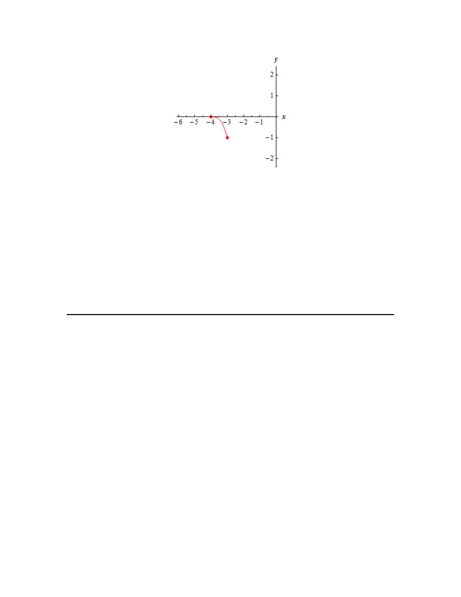
(c)

[

)

4, 3

− −

Here’s a graph of the function on this interval.

We still have no relative extrema for this function.

Because we are including the left endpoint in the interval we can see that we have an absolute

maximum at the point

(

)

4, 0

−

We need to be careful with the right endpoint however. It may look like we have an absolute

minimum at that point, but we don’t. We are not including

= −

in our interval. What this

means is that we are going to continue to take values of x that are closer and closer to

= −

and

graphing them, but we aren’t going to ever reach

= −

. Therefore, technically, the graph will

continually decreases without ever actually reaching a final value. It will get closer and closer to
-1, but will never actually reach that point. What this means for us is that there will be no
absolute minimum of the function on the given interval.

(d)

[

]

4, 3

− −

Here is a graph of the function on this interval.

Calculus I

http://tutorial.math.lamar.edu/terms.aspx

Note that the only difference between this part and the previous part is that we are now including
the right endpoint in the interval. Because of that most of the answers here are identical to part
(c).

There are no relative extrema of the function on the interval and there is an absolute maximum

at the point

(

)

4, 0

−

Now, unlike part (c) we are including

= −

in the interval and so the graph will reach a final

point, so to speak, as we move to the right. Therefore, for this interval, we have an absolute

minimum at the point

(

)

3, 1

− −

5. Sketch the graph of some function on the interval

[ ]

1, 6

that has an absolute maximum at

and an absolute minimum at

Hint :Do not let the apparent difficulty of this problem fool you. It’s not asking us to find an
actual function that meets these conditions. It’s only asking for a graph that meets the conditions
and we know what absolute extrema look like so just start sketching and keep in mind what the
conditions are.

Step 1
So, we need a graph of some function (not the function itself, only the graph). The graph must be

on the interval

[ ]

1, 6

and must have absolute extrema at the specified points.

By this point we should have seen enough sketches of graphs to have a pretty good idea of what
absolute minimums that are not at the endpoints of an interval should look like on a graph.

Therefore, we should know basically what the graph should look like at

Calculus I

http://tutorial.math.lamar.edu/terms.aspx

Next, we know that the absolute maximum must occur at the right end point of the interval and so
all we need to do is sketch a curve from the absolute minimum up to the right endpoint and make
sure that the graph at the right endpoint is simply higher than every other point on the graph.

For the graph to the left of the absolute minimum we can sketch in pretty much anything until we
reach the left end point, we just need to make sure that no portion of it goes below the absolute
minimum or above the absolute maximum.

Step 2
There are literally an infinite number of graphs that we could do here. Some will be more
complicated that others, but here is probably one of the simpler graphs that we could use here.

6. Sketch the graph of some function on the interval

[

]

4, 3

−

that has an absolute maximum at

= −

and an absolute minimum at

on the interval

[

]

4, 3

−

and must have absolute extrema at the specified points.

By this point we should have seen enough sketches of graphs to have a pretty good idea of what
absolute maximums/minimums that are not at the endpoints of an interval should look like on a

graph. Therefore, we should know basically what the graph should look like at

= −

and

Calculus I

http://tutorial.math.lamar.edu/terms.aspx

. There are many ways we could sketch the graph between these two points, but there is no

reason to overly complicate the graph so the best thing to do is probably just sketch in a short
smooth curve connecting the two points.

Also, because the absolute extrema occur interior to the interval we know that the graph at the
endpoints of the interval must fall somewhere between the maximum/minimum values of the
graph.  This means that as we sketch the graph from the absolute maximum to the left end point
we can sketch anything we just need to make sure it never rises above the highest point on the
graph or below the lowest point on the graph.

Similarly as we sketch the graph from the absolute minimum to the right endpoint we just need to
make sure it stays between the highest and lowest point on the graph.

Step 2
There are literally an infinite number of graphs that we could do here. Some will be more
complicated that others, but here is probably one of the simpler graphs that we could use here.

7. Sketch the graph of some function that meets the following conditions :

(a) The function is continuous.
(b) Has two relative minimums.
(b) One of relative minimums is also an absolute minimum and the other relative

minimum is not an absolute minimum.

(c) Has one relative maximum.
(d) Has no absolute maximum.

Calculus I

http://tutorial.math.lamar.edu/terms.aspx

and we know what absolute and relative extrema look like so just start sketching and keep in
mind what the conditions are.

Step 1
So, we need a graph of some function (not the function itself, only the graph) that meets the given
conditions. We were not given an interval as one of the conditions so it’s okay to assume that the

interval is

(

)

−∞ ∞

for this problem.

From the first condition we know that we can’t have any holes or breaks in the graph in order for
the function to be continuous.

Now let’s take care of the next two conditions as they are related to each other. By this point
we’ve seen enough sketches of graphs to have a pretty good idea of what absolute and relative
minimums looks like. So, we’re going to need two downwards pointing “bumps” in the graph to
give use the two relative minimums. Also, one of them must be the lowest point on the graph and
other must be higher so it is not also an absolute minimum.

Next, we want to think about how to connect the two relative minimums. This is also where the
fourth condition comes in. As we’ll see because we have a continuous function we’ll need that to
connect the two relative minimums.

Let’s start with the leftmost relative minimum. In order for it to be a minimum the graph must be
increasing as we move to the right. However, if we also want to get the minimum to the right of
this the graph will have to, at some point, start decreasing again. If you think about it that is
exactly what a relative maximum will look like. So, in moving from the leftmost relative
minimum to the rightmost relative minimum we must have a relative maximum between them
and so the fourth condition is automatically met.

Note that if we don’t insist on a continuous function it is possible to get from one to the other
without having a relative minimum. All it would take is to have a division by zero discontinuity
somewhere between the two relative minimums in which the graph goes to positive infinity on
both sides of the discontinuity.

This would maintain the relative minimums and at the same time would not be a relative
maximum.

Now let’s deal with the final condition.  In order for the graph to have no absolute maximum all
we really need to do is make sure that the graph increases without bound as we move to the right
and left of the graph.  This will also match up nicely with the relative minimums that we are
required to have.

To the left of the leftmost relative minimum the graph must be increasing and so we may as well
just let it increase forever on that side. Likewise, on the right side of the rightmost relative

Calculus I

http://tutorial.math.lamar.edu/terms.aspx

minimum the graph will need to be increasing. So, again let’s just let the graph increase forever
on that side.

Step 2
There are literally an infinite number of graphs that we could do here. Some will be more
complicated that others, but here is probably one of the simpler graphs that we could use here.

Finding Absolute Extrema

1. Determine the absolute extrema of

( )

f x

−

[

]

8, 2

−

Hint : Just recall the process for finding absolute extrema outlined in the notes for this section and
you’ll be able to do this problem!

Step 1
First, notice that we are working with a polynomial and this is continuous everywhere and so will
be continuous on the given interval. Recall that this is important because we now know that
absolute extrema will in fact exist by the

Extreme Value Theorem

Now that we know that absolute extrema will in fact exist on the given interval we’ll need to find
the critical points of the function.

Given that the purpose of this section is to find absolute extrema we’ll not be putting much
work/explanation into the critical point steps. If you need practice finding critical points please
go back and work some problems from that section.

Calculus I

http://tutorial.math.lamar.edu/terms.aspx

Here are the critical points for this function.

( )

(

)(

)

1
4

162

6 4

′

−

⇒

= −

Step 2
Now, recall that we actually are only interested in the critical points that are in the given interval
and so, in this case, the critical points that we need are,

1
4

= −

Step 3
The next step is to evaluate the function at the critical points from the second step and at the end
points of the given interval. Here are those function evaluations.

( )

1
4

1416

1511

13.3125

296

− =

= −

Do not forget to evaluate the function at the end points! This is one of the biggest mistakes that
people tend to make with this type of problem.

Step 4
The final step is to identify the absolute extrema. So, the answers for this problem are then,

1
4

Absolute Maximum : 1511 at

Absolute Minimum : 13.3125 at

= −

−

2. Determine the absolute extrema of

( )

f x

−

[

]

4, 2

−

Extreme Value Theorem

Now that we know that absolute extrema will in fact exist on the given interval we’ll need to find
the critical points of the function.

Calculus I

http://tutorial.math.lamar.edu/terms.aspx

Given that the purpose of this section is to find absolute extrema we’ll not be putting much
work/explanation into the critical point steps. If you need practice finding critical points please
go back and work some problems from that section.

Here are the critical points for this function.

( )

(

)(

)

1
4

162

6 4

′

−

⇒

= −

Step 2
Now, recall that we actually are only interested in the critical points that are in the given interval
and so, in this case, the only critical point that we need is,

1
4

Step 3
The next step is to evaluate the function at the critical point from the second step and at the end
points of the given interval. Here are those function evaluations.

( )

1
4

944

13.3125

296

− =

= −

1
4

Absolute Maximum : 944 at

Absolute Minimum : 13.3125 at

= −

−

Note the importance of paying attention to the interval with this problem. Had we neglected to

exclude

= −

we would have gotten the wrong answer for the absolute maximum (check out

the previous problem to see this….).

3. Determine the absolute extrema of

( )

1 80

R t

= +

−

[

]

4.5, 4

−

Hint : Just recall the process for finding absolute extrema outlined in the notes for this section and
you’ll be able to do this problem!

Step 1

Calculus I

http://tutorial.math.lamar.edu/terms.aspx

First, notice that we are working with a polynomial and this is continuous everywhere and so will
be continuous on the given interval. Recall that this is important because we now know that
absolute extrema will in fact exist by the

Extreme Value Theorem

( )

(

)(

)

240

R t

′

−

= −

−

⇒

= −

Step 2
Now, recall that we actually are only interested in the critical points that are in the given interval
and so, in this case, the critical points that we need are,

= −

Step 3
The next step is to evaluate the function at the critical points from the second step and at the end
points of the given interval. Here are those function evaluations.

(

)

( )

4.5

1548.13

1791

4353

−

= −

− = −

Absolute Maximum : 4353 at

Absolute Minimum : 1791 at

−

= −

Note the importance of paying attention to the interval with this problem. Had we neglected to

exclude

we would have gotten the wrong answer for the absolute maximum. Also note that

if we’d neglected to check the endpoints at all we also would have gotten the wrong absolute
maximum.

Calculus I

http://tutorial.math.lamar.edu/terms.aspx

4. Determine the absolute extrema of

( )

1 80

R t

= +

−

[ ]

0, 7

Extreme Value Theorem

( )

(

)(

)

240

R t

′

−

= −

−

⇒

= −

Step 2
Now, recall that we actually are only interested in the critical points that are in the given interval
and so, in this case, the critical points that we need are,

Do not get excited about the fact that one of the critical points also happens to be one of the end
points of the interval. This happens on occasion.

Step 3
The next step is to evaluate the function at the critical points from the second step and at the end
points of the given interval. Here are those function evaluations.

( )

8209

5832

Calculus I

http://tutorial.math.lamar.edu/terms.aspx

Absolute Maximum : 8209 at

Absolute Minimum : 1 at

Note the importance of paying attention to the interval with this problem. Had we neglected to

exclude

= −

we would have gotten the wrong answer for the absolute minimum.

5. Determine the absolute extrema of

( )

h z

−

[

]

2,1

−

Extreme Value Theorem

( )

396

h z

± −

′

−

+ =

⇒

Now, recall that we only work with real numbers here and so we ignore complex roots.
Therefore this function has no critical points.

Step 2
Technically the next step is to determine all the critical points that are in the given interval.
However, there are no critical points for this function and so there are also no critical points in the
given interval.

Step 3
The next step is to evaluate the function at the critical points from the second step and at the end
points of the given interval. However, since there are no critical points for this function all we
need to do is evaluate the function at the end points of the interval.

Calculus I

http://tutorial.math.lamar.edu/terms.aspx

Here are those function evaluations.

( )

− = −

Do not forget to evaluate the function at the end points! This is one of the biggest mistakes that
people tend to make with this type of problem. That is especially true for this problem as there
would be no points to evaluate at without the end points.

Step 4
The final step is to identify the absolute extrema. So, the answers for this problem are then,

Absolute Maximum : 22 at

Absolute Minimum : 50 at

−

= −

Note that if we hadn’t remembered to evaluate the function at the end points of the interval we
would not have had an answer for this problem!

6. Determine the absolute extrema of

( )

g x

−

[ ]

1, 5

Extreme Value Theorem

( )

(

)(

)

5
2

120

4 2

g x

x x

′

−

− =

⇒

Step 2

Calculus I

http://tutorial.math.lamar.edu/terms.aspx

Now, recall that we actually are only interested in the critical points that are in the given interval
and so, in this case, the critical points that we need are,

5
2

Step 3
The next step is to evaluate the function at the critical points from the second step and at the end
points of the given interval. Here are those function evaluations.

( )

5
2

74.9375

114

Absolute Maximum : 114 at

Absolute Minimum : 26 at

Note that if we hadn’t remembered to evaluate the function at the end points of the interval we
would have gotten both of the answers incorrect!

7. Determine the absolute extrema of

( ) (

)

(

)

2 8

Q x

−

[

]

3, 3

−

Extreme Value Theorem

Calculus I

http://tutorial.math.lamar.edu/terms.aspx

Here are the critical points for this function.

( ) ( )(

)

(

)

( )(

)

(

)

(

)

(

) (

)

5796

1
4

8 2 8

3 2

2 8

4 2 8

1.8239, 1.9739

Q x

′

= −

−

= −

−

⇒

= ±

= −

Step 2
Now, recall that we actually are only interested in the critical points that are in the given interval
and so, in this case, we need all the critical points from the first step.

5796

1
4

1.8239, 1.9739

= ±

= −

Do not get excited about the fact that both end points of the interval are also critical points. It
happens sometimes and in this case it will reduce the number of computations required in the next
step by 2 and that’s not a bad thing.

Step 3
The next step is to evaluate the function at the critical points from the second step and at the end
points of the given interval. Here are those function evaluations.

( )

(

)

( )

(

)

( )

1
4

1.8239

1.38 10

1.9739

4.81 10

− =

−

= −

Do not get excited about the large numbers for the two non-zero function values. This is
something that is going to happen on occasion and we shouldn’t worry about it when it does
happen.

Step 4
The final step is to identify the absolute extrema. So, the answers for this problem are then,

1
4

Absolute Maximum : 0 at

Absolute Minimum : 1.38 10 at

1.8239

= −

−

= −

Recall that while we can only have one largest possible value (i.e. only one absolute maximum) it
is completely possible for it to occur at more than one point (3 points in this case).

8. Determine the absolute extrema of

( )

(

)

h w

−









Calculus I

http://tutorial.math.lamar.edu/terms.aspx

Extreme Value Theorem

( )

(

)

(

)

(

) (

)

3
4

h w

w w

′

+ =

⇒

= −

Step 2
Now, recall that we actually are only interested in the critical points that are in the given interval
and so, in this case, we need all the critical points from the first step.

3
4

= −

Step 3
The next step is to evaluate the function at the critical points from the second step and at the end
points of the given interval. Here are those function evaluations.

( )

0.9766

2.5749

24.4141

− =

− = −

Step 4
The final step is to identify the absolute extrema. So, the answers for this problem are then,

1
2

3
4

Absolute Maximum : 24.4141 at

Absolute Minimum :

2.5749 at

−

= −

Calculus I

http://tutorial.math.lamar.edu/terms.aspx

9. Determine the absolute extrema of

( )

f z

+ +

[

]

10, 0

−

Hint : Just recall the process for finding absolute extrema outlined in the notes for this section and
you’ll be able to do this problem!

Step 1
First, notice that we are working with a rational expression in which both the numerator and
denominator are continuous everywhere. Also notice that the rational expression exists at all
points in the interval and so will be continuous on the given interval.  Recall that this is important
because we now know that absolute extrema will in fact exist by the

Extreme Value Theorem

( )

(

)

(

)(

)

(

)

(

)

(

)

1 2

4 4

4 3 2

8.2426, 0.2426

− ±

+ + − +

′

+ +

−

⇒

= − ±

= −

+ +

Step 2
Now, recall that we actually are only interested in the critical points that are in the given interval
and so, in this case, the only critical point that we need is,

4 3 2

8.2426

= − −

= −

Step 3
The next step is to evaluate the function at the critical point from the second step and at the end
points of the given interval. Here are those function evaluations.

(

)

(

)

( )

0.0303

8.2426

0.03128

−

= − = −

−

= −

Step 4
The final step is to identify the absolute extrema. So, the answers for this problem are then,

Calculus I

http://tutorial.math.lamar.edu/terms.aspx

1
2

Absolute Maximum : at

Absolute Minimum : 0.03128 at

4 3 2

−

= − −

Note the importance of paying attention to the interval with this problem. Had we neglected to

exclude

4 3 2

0.2426

= − +

we would have gotten the wrong answer for the absolute

maximum.

This problem also shows that we need to be very careful with doing too much rounding of our
answers. Had we rounded down to say 2 decimal places we would have been tempted to say that
the absolute minimum occurred at two places when in fact one of the points was lower than the
other.

10. Determine the absolute extrema of

( )

(

)

A t

−

[

]

2, 10.5

Hint : Just recall the process for finding absolute extrema outlined in the notes for this section and
you’ll be able to do this problem!

Step 1
First, notice that we are working with a product of a polynomial and a cube root function. Bother
are continuous everywhere and so the product will be continuous on the given interval. Recall
that this is important because we now know that absolute extrema will in fact exist by the

Extreme Value Theorem

( )

(

)

( )

( )(

)

(

)

(

)

(

)

(

)

(

)

(

)

(

)

2 10

1 10

2 10

3 10

6 10

4 15 2

3 10

A t

−

′

−

− −

−

Calculus I

http://tutorial.math.lamar.edu/terms.aspx

Don’t forget about critical points where the derivative doesn’t exist!

Step 2
Now, recall that we actually are only interested in the critical points that are in the given interval
and so, in this case, the critical points that we need are,

Step 3
The next step is to evaluate the function at the critical points from the second step and at the end
points of the given interval. Here are those function evaluations.

( )

(

)

103.613

10.5

69.4531

Step 4
The final step is to identify the absolute extrema. So, the answers for this problem are then,

Absolute Maximum : 103.613 at

Absolute Minimum : 0 at

Note the importance of paying attention to the interval with this problem. Had we neglected to

exclude

we would have had the absolute minimum showing up at two places instead of

only the one place inside the given interval.

11. Determine the absolute extrema of

( )

sin

f y

[

]

10,15

−

Hint : Just recall the process for finding absolute extrema outlined in the notes for this section and
you’ll be able to do this problem!

Step 1
First, notice that we are working with the sine function and this is continuous everywhere and so
will be continuous on the given interval. Recall that this is important because we now know that
absolute extrema will in fact exist by the

Extreme Value Theorem

Now that we know that absolute extrema will in fact exist on the given interval we’ll need to find
the critical points of the function.

Calculus I

http://tutorial.math.lamar.edu/terms.aspx

( )

cos

2.3005

−

′

+ =

→

= −

→

− =

2.3005 2

6.9016 6

0, 1, 2, ,

11.9481 6

3.9827

⇒

= ± ± ±



If you need some review on solving trig equations please go back to the Review chapter and work
some of the problems the Solving Trig Equations sections.

Step 2
Now, recall that we actually are only interested in the critical points that are in the given interval
and so, in this case, the critical points that we need are,

6.9016,

11.9481

= −

Note that we got these values by plugging in values of n into the solutions above and checking the
results against the given interval.

Step 3
The next step is to evaluate the function at the critical points from the second step and at the end
points of the given interval. Here are those function evaluations.

(

)

(

)

(

)

(

)

( )

2.0317

6.9016

2.2790

6.9016

2.2790

11.9481

1.9098

2.3744

−

= −

−

= −

Step 4
The final step is to identify the absolute extrema. So, the answers for this problem are then,

Absolute Maximum : 2.3744 at

Absolute Minimum :

2.2790 at

6.9016

−

= −

Note the importance of paying attention to the interval with this problem. Without an interval we
would have had (literally) an infinite number of critical points to check. Also, without an interval
(as a quick graph of the function would show) there would be no absolute extrema for this
function.

Calculus I

http://tutorial.math.lamar.edu/terms.aspx

12. Determine the absolute extrema of

( )

g w

−

= e

1
2

−









Hint : Just recall the process for finding absolute extrema outlined in the notes for this section and
you’ll be able to do this problem!

Step 1
First, notice that we are working with an exponential function with a polynomial in the exponent.
The exponent is continuous everywhere and so we can see that the exponential function will also
be continuous everywhere.  Therefore the function will be continuous on the given interval.
Recall that this is important because we now know that absolute extrema will in fact exist by the

Extreme Value Theorem

( )

(

)

(

)(

)

7
3

1 3

g w

−

′

−

⇒

= −

Step 2
Now, recall that we actually are only interested in the critical points that are in the given interval
and so, in this case, the only critical point that we need is,

7
3

Step 3
The next step is to evaluate the function at the critical point from the second step and at the end
points of the given interval. Here are those function evaluations.

( )

392

115

1
2

−

− =

Step 4
The final step is to identify the absolute extrema. So, the answers for this problem are then,

Calculus I

http://tutorial.math.lamar.edu/terms.aspx

392

1
2

7
3

Absolute Maximum :

Absolute Minimum :

−

= −

Note the importance of paying attention to the interval with this problem. Had we neglected to

exclude

= −

we would have gotten the absolute maximum wrong.

Also note that we need to be careful with rounding with this problem. Both of the exponentials
with negative exponents are very small and rounding could cause some real issues here.
However, we don’t need to actually do any calculator work for this anyway. Recall that the more
negative the exponent is the smaller the exponential will be.

So, because

392

115

we must have

392

115

−

13. Determine the absolute extrema of

( )

(

)

R x

[

]

4, 2

−

Hint : Just recall the process for finding absolute extrema outlined in the notes for this section and
you’ll be able to do this problem!

Step 1
First, notice that we are working with a logarithm whose argument is a polynomial (which is
continuous everywhere) that is always positive in the interval. Because of this we can see that the
function will be continuous on the given interval. Recall that this is important because we now
know that absolute extrema will in fact exist by the

Extreme Value Theorem

( )

R x

′

⇒

= −

Step 2
Now, recall that we actually are only interested in the critical points that are in the given interval
and so, in this case, the critical point that we need is,

Calculus I

http://tutorial.math.lamar.edu/terms.aspx

= −

Step 3
The next step is to evaluate the function at the critical points from the second step and at the end
points of the given interval. Here are those function evaluations.

( )

2.6391

2.3026

3.2581

− =

Step 4
The final step is to identify the absolute extrema. So, the answers for this problem are then,

Absolute Maximum : 3.2581 at

Absolute Minimum : 2.3026 at

= −

The Shape of a Graph, Part I

1. The graph of a function is given below. Determine the open intervals on which the function
increases and decreases.

Solution
There really isn’t too much to this problem. We can easily see from the graph where the function
in increasing/decreasing and so all we need to do is write down the intervals.

(

)

(

)

(

)

( )

Increasing :

3,1 & 7,

Decreasing :

, 3

1, 7

−

∞

−∞ −

Calculus I

http://tutorial.math.lamar.edu/terms.aspx

Note as well that by open intervals we mean that we don’t include the end points in the interval.
For this problem that is important because at the end points we are at infinity or the function is
either not increasing or decreasing.

2. The graph of a function is given below. Determine the open intervals on which the function
increases and decreases.

Solution
There really isn’t too much to this problem. We can easily see from the graph where the function
in increasing/decreasing and so all we need to do is write down the intervals.

(

) ( )

(

)

( )

Increasing :

,1 ,

4,8 & 8,

Decreasing : 1, 4

−∞

∞

3. Below is the graph of the derivative of a function. From this graph determine the open
intervals in which the function increases and decreases.

Calculus I

http://tutorial.math.lamar.edu/terms.aspx

Hint : Be careful with this problem. The graph is of the derivative of the function and so we
don’t just write down intervals where the graph is increasing and decreasing. Recall how the
derivative tells us where the function is increasing and decreasing and this problem is not too bad.

Solution

We have to be careful and not do this problem as we did the first two practice problems. The
graph given is the graph of the derivative and not the graph of the function. So, the answer is not
just where the graph is increasing or decreasing.

Instead we need to recall that the sign of the derivative tells us where the function is increasing
and decreasing.  If the derivative is positive (i.e. its graph is above the x-axis) then the function is
increasing and if the derivative is negative (i.e. its graph is below the x-axis) then the function is
decreasing.

So, it is fairly clear where the graph is above/below the x-axis and so we have the following
intervals of increase/decrease.

(

)

(

)

(

)

(

)

Increasing :

7, 2

2, 5

Decreasing :

, 7

− −

−

−∞ −

∞

4. This problem is about some function. All we know about the function is that it exists
everywhere and we also know the information given below about the derivative of the function.
Answer each of the following questions about this function.

Calculus I

http://tutorial.math.lamar.edu/terms.aspx

( )

(

) (

)

( )

(

) ( )

0 on

5, 2 ,

2, 4 , 8,

0 on

, 5 , 4,8

′

− =

′

− −

−

∞

−∞ −

Hint : This problem is actually quite simple. Just keep in mind how critical points are defined
and how we can answer the last two parts from the derivative of the function.

(a) Identify the critical points of the function.

Okay, let’s recall the definition of a critical point. A critical point is any point in which the
function exists and the derivative is either zero or doesn’t exist.

We are given that the function exists everywhere (and in fact this part is why that in there at
all….) and so we don’t really need to worry about that part of the definition for this problem.

Also, from the given information about the derivative we can see that at every point the derivative
is either zero, positive or negative. In other words, the derivative will exist at every point.

So, all this means that the critical points of the function are those points were the derivative is
zero and we are given those in the information.

Therefore, the critical points of the function are,

= −

(b) Determine the open intervals on which the function increases and decreases.

There is really not a lot to this part. We know that the function will increase where the derivative
is positive and it will decrease where the derivative is negative. This positive and negative
information is clearly listed above in the given information so here are the increasing/decreasing
intervals for this function.

(

)

( )

(

) (

)

(

)

Increasing :

, 5

& 4,8

Decreasing :

5, 2 ,

2, 4 & 8,

−∞ −

− −

−

∞

(c) Classify the critical points as relative maximums, relative minimums or neither.

Okay, there isn’t a lot that we need to do here. We know that relative maximums are increasing
on the left and decreasing on the right and relative minimums are decreasing on the left and
increasing on the right. We have all the increasing/decreasing information from the second part
so here is the answer to this part.

Calculus I

http://tutorial.math.lamar.edu/terms.aspx

: Relative Maximum

: Neither

: Relative Minimum

: Relative Maximum

= −
= −
=
=

5. For

( )

f x

−

answer each of the following questions.

(a) Identify the critical points of the function.

We need the 1

derivative to get the critical points so here it is.

( )

(

)

(

)(

)

′

−

Now, recall that critical points are where the derivative doesn’t exist or is zero. Clearly this
derivative exists everywhere (it’s a polynomial….) and because we factored the derivative we can
easily identify where the derivative is zero. The critical points of the function are,

= −

(b) Determine the open intervals on which the function increases and decreases.

To determine the increase/decrease information for the function all we need is a quick number
line for the derivative. Here is the number line.

From this we get the following increasing/decreasing information for the function.

(

)

(

)

(

)

Increasing :

, 2

& 5,

Decreasing :

2, 5

−∞ −

∞

−

Calculus I

http://tutorial.math.lamar.edu/terms.aspx

(c) Classify the critical points as relative maximums, relative minimums or neither.

With the increasing/decreasing information from the previous step we can easily classify the
critical points using the 1

derivative test. Here is classification of the functions critical points.

: Relative Maximum

: Relative Minimum

= −
=

6. For

( )

50 40

h t

−

answer each of the following questions.

(a) Identify the critical points of the function.

We need the 1

derivative to get the critical points so here it is.

( )

(

)

(

)(

)

120

h t

′

−

= −

+ −

= −

−

= −

Calculus I

http://tutorial.math.lamar.edu/terms.aspx

From this we get the following increasing/decreasing information for the function.

(

)

( )

(

)

(

)

Increasing :

3, 0

& 0, 2

Decreasing :

, 3

−

−∞ −

∞

derivative test. Here is classification of the functions critical points.

: Relative Minimum

Neither

: Relative Maximum

= −
=
=

7. For

−

answer each of the following questions.

(a) Identify the critical points of the function.

We need the 1

derivative to get the critical points so here it is.

−

Now, recall that critical points are where the derivative doesn’t exist or is zero. Clearly this
derivative exists everywhere (it’s a polynomial….) and because the derivative can’t be factored in
this case we’ll need to do a quick quadratic formula to find where the derivative is zero. The
critical points of the function are,

0.78475, 2.54858

Calculus I

http://tutorial.math.lamar.edu/terms.aspx

From this we get the following increasing/decreasing information for the function.

(

) (

)

(

)

Increasing :

Decreasing :

−

−∞

∞

derivative test. Here is classification of the functions critical points.

0.78475

: Relative Maximum

2.54858

: Relative Minimum

−

8. For

( )

cos 3

p x

answer each of the following questions on

3
2

, 2

−









(a) Identify the critical points of the function.

We need the 1

derivative to get the critical points so here it is.

( )

3sin 3

p x

′

= −

Now, recall that critical points are where the derivative doesn’t exist or is zero. Clearly this
derivative exists everywhere (the sine function exists everywhere….) and so all we need to do is
set the derivative equal to zero and solve. We’re not going to show all of those details so if you
need to do some review of the process go back to the

Solving Trig Equations

sections for some

examples.

Here are all the critical points.

Calculus I

http://tutorial.math.lamar.edu/terms.aspx

0.2432

0, 1, 2, 3,

0.8040

= ± ± ±



Plugging in some n’s gives the following critical points in the interval

3
2

, 2

−









1.2904,

0.2432,

0.8040

= −

From this we get the following increasing/decreasing information for the function.

(

)

(

]

)

(

)

3
2

Increasing :

1.2904, 0.2432

& 0.8040, 2

Decreasing :

, 1.2904 & 0.2432, 0.8040

−

− −



Be careful with the end points of these intervals! We are working on the interval

3
2

, 2

−









and

we’ve done no work for increasing and decreasing outside of this interval and so we can’t say
anything about what happens outside of the interval.

(c) Classify the critical points as relative maximums, relative minimums or neither.

With the increasing/decreasing information from the previous step we can easily classify the
critical points using the 1

derivative test. Here is classification of the functions critical points.

1.2904

: Relative Minimum

0.2432

: Relative Maximum

0.8040

: Relative Minimum

= −
=
=

Calculus I

http://tutorial.math.lamar.edu/terms.aspx

As with the last step, we need to again recall that we are only working on the interval

3
2

, 2

−









and

the classifications given here are only for those critical points in the interval. There are, of
course, an infinite number of critical points outside of this interval and they can all be classified
as relative minimums or relative maximums provided we do the work to justify the
classifications.

9. For

( )

2 5

14 sin

R z

= −

−

answer each of the following questions on

[

]

10, 7

−

(a) Identify the critical points of the function.

We need the 1

derivative to get the critical points so here it is.

( )

5 7 cos

R z

′

= − −

Now, recall that critical points are where the derivative doesn’t exist or is zero. Clearly this
derivative exists everywhere (the cosine function exists everywhere….) and so all we need to do
is set the derivative equal to zero and solve. We’re not going to show all of those details so if you
need to do some review of the process go back to the

Solving Trig Equations

sections for some

examples.

Here are all the critical points.

4.7328 4

0, 1, 2, 3,

7.8336 4

π
π

= ± ± ±



Plugging in some n’s gives the following critical points in the interval

[

]

10, 7

−

7.8336,

4.7328,

4.7328

= −

Calculus I

http://tutorial.math.lamar.edu/terms.aspx

From this we get the following increasing/decreasing information for the function.

(

)

(

]

[

)

(

)

Increasing :

7.8336, 4.7328

& 4.7328, 7

Decreasing :

10, 7.8336 &

4.7328, 4.7328

−

Be careful with the end points of these intervals! We are working on the interval

[

]

10, 7

−

and

derivative test. Here is classification of the functions critical points.

7.8336

: Relative Minimum

4.7328

: Relative Maximum

4.7328

: Relative Minimum

= −
= −
=

As with the last step, we need to again recall that we are only working on the interval

[

]

10, 7

−

and the classifications given here are only for those critical points in the interval. There are, of
course, an infinite number of critical points outside of this interval and they can all be classified
as relative minimums or relative maximums provided we do the work to justify the
classifications.

10. For

( )

2 3

h t

−

answer each of the following questions.

(a) Identify the critical points of the function.

Calculus I

http://tutorial.math.lamar.edu/terms.aspx

We need the 1

derivative to get the critical points so here it is.

( )

(

)

( )

(

)

(

)

(

)

(

)

(

)

(

)

(

)

(

)

1
3

h t

t t

−

′

−

− +

−

Now, recall that critical points are where the derivative doesn’t exist or is zero. Because we
simplified and factored the derivative as much as possible we can clearly see that the derivative

does not exist at

(and the function exists here…) and that the derivative is zero at

and

. The critical points of this function are then,

From this we get the following increasing/decreasing information for the function.

(

) ( )

(

)

( )

Increasing :

, 0 ,

6, 7

& 7,

Decreasing : 0, 6

−∞

∞

derivative test. Here is classification of the functions critical points.

Calculus I

http://tutorial.math.lamar.edu/terms.aspx

: Relative Maximum

: Relative Minimum

: Neither

=
=
=

11. For

( )

f w

−

= e

answer each of the following questions.

(a) Identify the critical points of the function.

We need the 1

derivative to get the critical points so here it is.

( )

(

)

(

)(

)

−

′

−

Now, recall that critical points are where the derivative doesn’t exist or is zero. Because we
simplified and factored the derivative as much as possible we can clearly see that the derivative
will exist everywhere (it’s the product of functions that exist everywhere).  We can also easily see
where the derivative is zero. The critical points of this function are then,

= −

From this we get the following increasing/decreasing information for the function.

Calculus I

http://tutorial.math.lamar.edu/terms.aspx

(

)

(

)

( )

Increasing :

1,1

Decreasing :

, 1

−

−∞ −

∞

derivative test. Here is classification of the functions critical points.

: Relative Minimum

: Relative Maximum

= −
=

12. For

( )

(

)

2 ln 1

g x

= −

answer each of the following questions.

(a) Identify the critical points of the function.

We need the 1

derivative to get the critical points so here it is.

( )

1 4

1 2

g x

−

= −

Now, recall that critical points are where the derivative doesn’t exist or is zero. Because we
simplified and factored the derivative as much as possible we can clearly see that the derivative
will exist everywhere (or at least the denominator will not be zero for any real numbers…). We’ll
also need the quadratic formula to determine where the numerator, and hence the derivative, is
zero. The critical points of this function are then,

0.2679, 3.7321

= ±

Calculus I

http://tutorial.math.lamar.edu/terms.aspx

From this we get the following increasing/decreasing information for the function.

(

)

(

)

(

)

Increasing :

, 0.2679

3.7321,

Decreasing : 0.2679, 3.7321

−∞

∞

derivative test. Here is classification of the functions critical points.

0.2679

: Relative Maximum

3.7321

: Relative Minimum

=
=

13. For some function,

( )

f x

, it is known that there is a relative maximum at

. Answer

each of the following questions about this function.

(a) What is the simplest form for the derivative of this function?

Note : There really are many

possible forms of the derivative so to make the rest of this problem as simple as possible you will
want to use the simplest form of the derivative that you can come up with.

(b) Using your answer from (a) determine the most general form of the function.

(c) Given that

( )

find a function that will have a relative maximum at

Note :

You should be able to use your answer from (b) to determine an answer to this part.

Hint : As noted in the problem there are many possible forms that the derivative can take.
However, if we want things to remain simple just keep in mind what it takes for a point to be a
critical point (why a critical point?). With that in mind it should be pretty simple to figure out a
really simple form for the derivative to take to make sure we get a relative maximum at the point.

(a) What is the simplest form for the derivative of this function?

Note : There really are many

possible forms of the derivative so to make the rest of this problem as simple as possible you will want
to use the simplest form of the derivative that you can come up with.

Okay, let’s get started with this problem.

Calculus I

http://tutorial.math.lamar.edu/terms.aspx

The first thing that we’ll do is assume that the derivative exists everywhere. Making assumptions
in a math class is generally a bad thing. However, in this case, because we are being asked to
come up the form of the derivative all we are really doing here is starting that process. If we
can’t find a derivative that will have a relative maximum at the point that also exists everywhere
we can come back and change things up. If we can find a derivative that will exist everywhere
(which we can as we’ll see) this assumption will help with keeping the derivative as simple as
possible.

Now, given that we are assuming that the derivative exists everywhere and we know that if we

have a relative maximum at

then

must also be a critical point (recall

Fermat’s

Theorem

from a couple of sections ago…). This is another reason for the assumption we made

above. Fermat’s theorem requires that the derivative exist at the point in order to know that it is
also a critical point.

Next, because we assumed that the derivative exists everywhere (and in particular it exists at

) we know that in order for it to be a critical point we must also have

( )

f ′

. There are

lots and lots of functions that will be zero at

but probably one of the simplest is use,

( )

′

= −

This does give

( )

f ′

as we need, however we have a problem. We can clearly see that if

we would have

( )

′

and if

we would have

( )

′

. This says that

would have to be a relative minimum and not the relative maximum that we wanted it to be.

Luckily enough for us this is easy to fix. The only problem with our original guess is that the

signs of the derivative to the right and left of

are opposite what we need them to be.

Therefore, all we need to do is change them and that can easily be done by multiplying by a
negative or,

( )

′

= −

With this choice we still have

( )

f ′

and now the derivative is positive if

and negative

which means that

will be a relative maximum.

As noted in the problem statement there are many possible answers to this part. We will be
working with the one given above. However, just to make the point here are a sampling of other

derivatives all of which come from functions that have a relative maximum at

( )

(

)

24 18

sin 2

π π

−

′

−

Calculus I

http://tutorial.math.lamar.edu/terms.aspx

After working the rest of this problem with

( )

′

= −

you might want to come back and see

if you can repeat the problem with one or more of these to see what you get.

Hint : This is where the problem gets a little tricky (as if the previous part wasn’t tricky huh?).
What we need to do here is “undo” the derivative. However, if you kept the answer from the
previous part simple and you understand how differentiation works then it shouldn’t be too hard
to “undo” the differentiation and determine a function that gives your derivative. Keep in mind
however that the problem statement asks for the most general possible function and that is where
most will run into problems with this part.

(b) Using your answer from (a) determine the most general form of the function.

Okay, from the previous part we have assumed that the derivative of our function is

( )

′

= −

and we need to “undo” the differentiation to determine the most general possible

function that we could have had.

So, before doing this let’s recall what we know about differentiation. First, let’s recall the
following formula,

( )

−

When we differentiate a power of x the power goes down by one. So, what would we have to
differentiate to get x? We’ll, since the exponent on the x is 1 we would have had to differentiate

. However, because we know that that the derivative of

is 2x and we want just an x that

would mean that in fact we would have had to differentiate

1
2

to get x.

Next, also recall,

( )

So, using this as a guide is should be pretty simple to see that we would need to differentiate 4x to
get 4.

So, if we put these two parts together it looks like we could use the following function.

( )

1
2

f x

−

The derivative of this function is clearly

( )

′

= −

. However, it is not the most general

possible function that gives this derivative.

Calculus I

http://tutorial.math.lamar.edu/terms.aspx

Do not forget that the derivative of a constant is zero and so we could add any constant onto our
function and get the same derivative.

This is one of the biggest mistakes that students make with learning to “undo” differentiation.
Any time we undo differentiation there is always the possibility that there was a constant on the
original function and so we need to acknowledge that.  We usually do this by adding a “ + c ”
onto the end of our function. We use a general c because we have no way of knowing that the
constant would be and this allows for all possible constants.

Therefore, the most general function that we could use to get

( )

′

= −

is,

( )

1
2

f x

−

Hint : This is the “easy” part of this problem. All we are really being asked to do is determine the

specific value of c that we would need in order have the function have the value of 1 at

. If

you’ve reached this point of a Calculus course you should have the required Algebra knowledge
(and yes it really is just Algebra) to do this part.

(c) Given that

( )

find a function that will have a relative maximum at

Note : You

should be able to use your answer from (b) to determine an answer to this part.

To do this part all we really need to do is plug

into our answer from the previous part and

set the result equal to 1. This will result in an equation with a single unknown value, c. So all we
need to do then is solve for c.

Here is the work for this part.

( )

( ) ( )

1
2

4 4

1 8

−

+ = +

→

= +

→

= −

So, it looks like one possible function that will have a relative maximum at

is,

( )

1
2

f x

−

As a final part to this problem, here is a quick graph of this function to verify that it does in fact

have a relative maximum at

Calculus I

http://tutorial.math.lamar.edu/terms.aspx

14. Given that

( )

f x

and

( )

g x

are increasing functions. If we define

( )

( ) ( )

h x

f x

g x

show that

( )

h x

is an increasing function.

Hint : At first glance this problem may seem quite difficult. However, just keep in mind how we
have been determining whether functions where increasing to this point and that should suggest a
first step.

Step 1
To this point we’ve always used the derivative to determine if a function was increasing so let’s
do that here as well.

Note that this may not seem all that useful because we don’t actually know what any of the
functions are. However, just because we don’t know what the functions are doesn’t mean that we

can’t at least write down a formula for

( )

h x

′

. Here is that formula.

( )

h x

g x

′

Hint : We were told that

( )

f x

and

( )

g x

are increasing functions so what does that tell us about

their derivatives?

Step 2

We are told that both

( )

f x

and

( )

g x

are increasing functions so this means that we know that

both of their derivatives must be positive. Or,

( )

g x

′

Calculus I

http://tutorial.math.lamar.edu/terms.aspx

Hint : Given the formula for

( )

h x

′

we found in Step 1 and what we noticed about the signs of

( )

′

and

( )

g x

′

that we noted in Step 2 what can we say about the sign of

( )

h x

Step 3
Okay, we are pretty much done at this point. We know from Step 1 that,

( )

h x

g x

′

Also from Step 2 we know that both

( )

′

and

( )

g x

′

are positive. So,

( )

h x

′

is the sum of

two positive functions and in turn means that we must have,

( )

h x

′

Therefore we can see that

( )

h x

must be an increasing function.

-------------------------------------------------------

Final Thoughts / Strategy Discussion
Figuring out how to do these kinds of problems can definitely seem quite daunting at times. That
is especially true when the statement we are being asked to prove seems to be fairly "obvious" as
is the case here. The sum of two increasing functions intuitively should also be increasing. The
problem is that we are being asked to actually prove that and not just say "well it makes sense so
it should be true".

What we want to discuss here is not the proof of this fact (that is given above after all...). Instead
let's take a look at the thought process that went into constructing the proof above.

The first step is to really look at what we are being asked to prove.  This means not just reading
the statement, but reading the statement and trying to relate what we are being asked to prove to
something we already know.

In this case, we’re being asked to show that a general function is increasing given a set of
assumptions. By this point we know how to prove that specific functions are increasing.  So, let’s
start with that.

We know that in order to use Calculus to prove that a function is increasing we need to look at the
derivative of the function.  We also know that, at least symbolically, we write down the formula
for the derivative of the function we are interested in for this problem.

Now for the next step in the thought process.  We've got a formula and we know that we need to
show that it is positive.  At this point we need to think about the assumptions that we were given.

Calculus I

http://tutorial.math.lamar.edu/terms.aspx

Don't forget the assumptions. They were given for a reason and we'll need to use them. What do
the assumptions tell us? How can we relate them to what we are being asked to prove?

In this case, we know from the assumptions that the two derivatives were positive.

For this problem this wasn't a particularly difficult step, but for other problems this can be a little
tricky.

Finally, we need to put the two previous thought process steps together.  This can also be a fairly
tricky step. If you haven't had a lot of exposure to "mathematical logic/proofs" it can be daunting
to put all the information together. Often times you will need to try various ways of putting the
information together before something "clicks" and you can see how to proceed.  You may even
need to go back to the previous step and see if there is something about the assumptions that you
may have missed.

In this case we could see that the derivative was the sum of two other derivatives and from our
assumptions we knew that the two individual derivatives had to be positive. We also know from
basic Algebra knowledge that the sum of two positive quantities has to be positive and so we are
done.

The key part of this whole process is that you will have to persevere.  Try not to get discouraged
and if something doesn't work out move on and try something else. Also, do not get so wrapped
up in the process that you don't take breaks occasionally. If you keep running into road blocks
then step away for a while and come back at a later point. Sometimes that is all it takes to get a
fresh idea.

Another thing that students often initially have difficulty with is trying to mathematically write
this kind of thing down. In your mind you may have been able to see all the "logic" involved in
the proof, but just couldn't see who to put it all together and write it down.  If you are having that
problem the best thing to do is just start writing things down.

For instance, you know you need the derivative of the given function so write that down. If you
don't have a specific function to differentiate can you at least symbolically write down the
derivative as we did here?

Once you have that written down look at the pieces and start writing down what you know about

them. Actually write down what you know (i.e. things like

( )

′

). This seems silly at

times, but it really can help with the process.

Once you have everything written down you might be able to see how to string everything
together with words/explanations to prove what you want to prove.

Calculus I

http://tutorial.math.lamar.edu/terms.aspx

15. Given that

( )

f x

is an increasing function and define

( )

h x

f x

= 







. Will

( )

h x

be an

increasing function? If yes, prove that

( )

h x

is an increasing function. If not, can you determine

any other conditions needed on the function

( )

f x

that will guarantee that

( )

h x

will also

increase?

Hint : If you have trouble with these kinds of “proof” problems you might want to check out the
discussion at the end of the previous problem for a “strategy” that might be useful here.  This
isn’t quite the same kind of problem but the strategy given there should help here as well.

Hint : How do we use Calculus to determine if a function is increasing?

Step 1
We know that the derivative can be used to tell us if a function is increasing so let’s find the

derivative of

( )

h x

. Do not get excited about the fact that we don’t know what

( )

f x

is. We

can symbolically take the derivative with a quick application of the chain rule.

Here is the derivative of

( )

h x

( )

( ) ( )

h x

f x

f x f

′









Hint : How do we use the derivative to determine if a function is increasing?

Step 2
We know that a function will be increasing if its derivative is positive. So, the question we need

to answer is can we guarantee that

( )

h x

′

if we only take into account the assumption that

( )

f x

is an increasing function.

From our assumption that

( )

f x

is an increasing function and so we know that

( )

′

Now, let’s see what

( )

h x

′

tells us. We can see that

( )

h x

′

is a product of a number and two

functions. The “2” is positive and so the sign of the derivative will come from the sign of the

product of

( )

f x

and

( )

′

Hint : So, will

( )

h x

′

be positive?

Step 3

Calculus I

http://tutorial.math.lamar.edu/terms.aspx

Okay, from our assumption we know that

( )

′

is positive. However, the product isn’t

guaranteed to be positive.

For example, consider

( )

f x

. Clearly,

( )

1 0

′

= >

, and so this is an increasing function.

However,

( ) ( ) ( )( )

f x f

′

. Therefore, we can see that the product will not always be

positive. This shouldn’t be too surprising given that,

( )

[ ]

h x

f x









In this case we can clearly see that

( )

h x

will not always be an increasing function.

On the other had if we let

( )

f x

= e

we can see that

( )

′

and we can also see that

( ) ( )

( )( )

f x f

′

So, from these two examples we can see that we can find increasing functions,

( )

f x

, for which

( )

f x









may or may not always be increasing.

Hint : Can you use the examples above to determine a condition on

( )

f x

that will guarantee that

( )

h x

will be increasing?

Step 4
So, just what was the difference between the two examples above?

The problem with the first example,

( )

f x

was that it wasn’t always positive and so the

product of

( )

f x

and

( )

′

would not always be positive as we needed it to be.

This was not a problem with the second example however,

( )

f x

= e

. In this case the function

is always positive and so the product of the function and its derivative will also be positive.

That is also the added condition that we need to guarantee that

( )

h x

will be positive.

If we start with the assumption that

( )

f x

in an increasing function we need to further assume

that

( )

f x

is a positive function in order to guarantee that

( )

h x

f x

= 







will be a positive

function.

Calculus I

http://tutorial.math.lamar.edu/terms.aspx

The Shape of a Graph, Part II

1. The graph of a function is given below. Determine the open intervals on which the function is
concave up and concave down.

Solution
There really isn’t too much to this problem.  We can easily see from the graph where the function
in concave up/concave down and so all we need to do is estimate where the concavity changes
(and this really will be an estimate as it won’t always be clear) and write down the intervals.

(

)

(

)

(

)

( )

Concave Up :

1, 2 & 6,

Concave Down :

, 1

2, 6

−

∞

−∞ −

Again, the endpoints of these intervals are, at best, estimates as it won’t always be clear just
where the concavity changes.

2. Below is the graph the 2

derivative of a function. From this graph determine the open

intervals in which the function is concave up and concave down.

Calculus I

http://tutorial.math.lamar.edu/terms.aspx

Hint : Be careful with this problem. The graph is of the 2

derivative of the function and so we

don’t just write down intervals where the graph is concave up and concave down. Recall how the
2

derivative tells us where the function is concave up and concave down and this problem is not

too bad.

Solution
We need to be careful and not do this problem as we did the first practice problem. The graph
given is the graph of the 2

derivative and not the graph of the function. Therefore, the answer

is not just where the graph is concave up or concave down.

What we need to do here is to recall that if the 2

derivative is positive (i.e. the graph is above the

x-axis) then the function in concave up and if the 2

derivative is negative (i.e. the graph is below

the x-axis) then the function is concave down.

So, it is fairly clear where the graph is above/below the x-axis and so we have the following
intervals of concave up/concave down.

(

) (

)

(

)

(

)

Concave Up :

, 4 ,

2, 3 & 3,

Concave Down :

4, 2

−∞ −

−

∞

− −

Even though the problem didn’t ask for it we can also identify that

= −

and

= −

are

inflection points because at these points the concavity changes. Note that

is not an

inflection point. Clearly the 2

derivative is zero here, but the concavity doesn’t change at this

point and so it is not an inflection point. Keep in mind inflection points are only where the
concavity changes and not simply where the 2

derivative is zero.

3. For

( )

12 6

f x

−

answer each of the following questions.

Calculus I

http://tutorial.math.lamar.edu/terms.aspx

(a) Determine a list of possible inflection points for the function.
(b) Determine the open intervals on which the function is concave up and concave down.
(c) Determine the inflection points of the function.

(a) Determine a list of possible inflection points for the function.

To get the list of possible inflection points for the function we’ll need the 2

derivative of the

function so here that is.

( )

12 6

′

′′

−

Now, recall that possible inflection points are where the 2

derivative either doesn’t exist or is

zero. Clearly the 2

derivative exists everywhere (it’s a polynomial….) and, in this case, it

should be fairly clear where the 2

derivative is zero. The only possible inflection critical point of

the function in this case is,

(b) Determine the open intervals on which the function is concave up and concave down.

There isn’t much to this part. All we really need here is a number line for the 2

derivative. Here

that is,

From this we get the following concave up/concave down information for the function.

(

)

(

)

Concave Up :

, 2

Concave Down : 2,

−∞

∞

(c) Determine the inflection points of the function.

For this part all we need to do is interpret the results from the previous step. Recall that inflection
points are points where the concavity changes (as opposed to simply the points where the 2

derivative is zero or doesn’t exist). Therefore the single inflection point for this function is,

Calculus I

http://tutorial.math.lamar.edu/terms.aspx

4. For

( )

g z

−

answer each of the following questions.

(a) Determine a list of possible inflection points for the function.

To get the list of possible inflection points for the function we’ll need the 2

derivative of the

function so here that is.

( )

(

)

g z

z z

′

′′

−

Now, recall that possible inflection points are where the 2

derivative either doesn’t exist or is

zero. Clearly the 2

derivative exists everywhere (it’s a polynomial….) and, because we factored

the 2

derivative, it should be fairly clear where the 2

derivative is zero. The possible inflection

critical points of this function are,

(b) Determine the open intervals on which the function is concave up and concave down.

There isn’t much to this part. All we really need here is a number line for the 2

derivative. Here

that is,

From this we get the following concave up/concave down information for the function.

(

)

(

)

( )

Concave Up :

, 0

Concave Down : 0, 6

−∞

∞

Calculus I

http://tutorial.math.lamar.edu/terms.aspx

derivative is zero or doesn’t exist). Therefore the inflection points for this function are,

5. For

( )

h t

= +

−

answer each of the following questions.

(a) Determine a list of possible inflection points for the function.

To get the list of possible inflection points for the function we’ll need the 2

derivative of the

function so here that is.

( )

(

)

12 12

h t

′

′′

−

+ +

Now, recall that possible inflection points are where the 2

derivative either doesn’t exist or is

zero. Clearly the 2

derivative exists everywhere (it’s a polynomial….). In this case the 2

derivative doesn’t factor and so we’ll need to use the quadratic formula to determine where the
2

derivative is zero.

The possible inflection critical points of this function are,

3 2 2

5.8284,

0.1716

= − ±

= −

−

(b) Determine the open intervals on which the function is concave up and concave down.

There isn’t much to this part. All we really need here is a number line for the 2

derivative. Here

that is,

Calculus I

http://tutorial.math.lamar.edu/terms.aspx

From this we get the following concave up/concave down information for the function.

(

)

(

)

(

)

Concave Up :

, 3 2 2

3 2 2,

Concave Down :

3 2 2, 3 2 2

−∞ − −

− +

∞

− −

− +

derivative is zero or doesn’t exist). Therefore the inflection points for this function are,

3 2 2

= − −

= − +

6. For

( )

8 5

cos 3

h w

= −

−

[

]

1, 2

−

answer each of the following questions.

(a) Determine a list of possible inflection points for the function.

To get the list of possible inflection points for the function we’ll need the 2

derivative of the

function so here that is.

( )

5 4

3sin 3

4 9 cos 3

h w

′

′′

= − +

= +

Now, recall that possible inflection points are where the 2

derivative either doesn’t exist or is

zero. Clearly the 2

derivative exists everywhere (the cosine function exists everywhere…) and

so all we need to do is set the 2

derivative equal to zero and solve. We’re not going to show all

Calculus I

http://tutorial.math.lamar.edu/terms.aspx

of those details so if you need to do some review of the process go back to the

Solving Trig

Equations

sections for some examples.

The possible inflection critical points of this function are,

0.6771

0, 1, 2, 3,

1.4173

= ± ± ±



Plugging in some n’s gives the following possible inflection points in the interval

[

]

1, 2

−

0.6771

1.4173

= −

(b) Determine the open intervals on which the function is concave up and concave down.

There isn’t much to this part. All we really need here is a number line for the 2

derivative. Here

that is,

From this we get the following concave up/concave down information for the function.

(

)

(

]

[

)

(

)

Concave Up :

0.6771, 0.6771

1.4173, 2

Concave Down :

0.6771

0.6771, 1.4173

−

− −

Be careful with the end points of these intervals! We are working on the interval

[

]

1, 2

−

and

we’ve done no work for concavity outside of this interval and so we can’t say anything about
what happens outside of the interval.

(c) Determine the inflection points of the function.

For this part all we need to do is interpret the results from the previous step. Recall that inflection
points are points where the concavity changes (as opposed to simply the points where the 2

derivative is zero or doesn’t exist). Therefore the inflection points for this function are,

Calculus I

http://tutorial.math.lamar.edu/terms.aspx

0.6771

1.4173

= −

As with the previous step we have to be careful and recall that we are working on the interval

[

]

1, 2

−

. There are infinitely many more possible inflection points and we’ve done no work

outside of the interval to determine if they are in fact inflection points!

7. For

( ) (

)

R z

z z

answer each of the following questions.

(a) Determine a list of possible inflection points for the function.

To get the list of possible inflection points for the function we’ll need the 2

derivative of the

function so here that is.

( ) (

)

( )

(

)

(

)

( )

(

)

(

)

(

)(

)

(

)

(

) (

)

(

)

(

)

2
3

5 3

R z

−

′

−









′′













Note that we simplified the derivatives at each step to help with the next step. You don’t
technically need to do this, but having the 2

derivative in its “simplest” form will definitely help

with getting the answer to this part.

Now, recall that possible inflection points are where the 2

derivative either doesn’t exist or is

zero. Because we simplified the 2

derivative as much as possible it is clear that the 2

derivative won’t exist at

= −

(and the function exists at this point as well!). It should also be

clear that the 2

derivative is zero at

= − = −

The possible inflection critical points of this function are then,

4.8

= − = −

= −

(b) Determine the open intervals on which the function is concave up and concave down.

Calculus I

http://tutorial.math.lamar.edu/terms.aspx

There isn’t much to this part. All we really need here is a number line for the 2

derivative. Here

that is,

From this we get the following concave up/concave down information for the function.

(

)

(

)

(

)

Concave Up :

, 4

Concave Down :

−

− ∞

−∞ −

derivative is zero or doesn’t exist). Therefore the only inflection point for this function is,

= −

8. For

( )

h x

−

= e

answer each of the following questions.

(a) Determine a list of possible inflection points for the function.

To get the list of possible inflection points for the function we’ll need the 2

derivative of the

function so here that is.

( )

(

)

2 4

h x

−

′

′′

= −

−

Don’t forget to product rule for the 2

derivative and factoring the exponential out will help a

little with the next step.

Calculus I

http://tutorial.math.lamar.edu/terms.aspx

Now, recall that possible inflection points are where the 2

derivative either doesn’t exist or is

zero. It should be fairly clear that the 2

derivative exists everywhere (it is a product of two

functions that exist everywhere…). We also know that exponentials are never zero and so the 2

derivative will be zero at the solutions to

− =

The possible inflection critical points of this function are then,

0.7071

= ±

(b) Determine the open intervals on which the function is concave up and concave down.

There isn’t much to this part. All we really need here is a number line for the 2

derivative. Here

that is,

From this we get the following concave up/concave down information for the function.

(

)

(

)

(

)

Concave Up :

Concave Down :

−∞ −

∞

−

derivative is zero or doesn’t exist). Therefore the only inflection point for this function is,

0.7071

= −

9. For

( )

g t

= −

answer each of the following questions.

(a) Identify the critical points of the function.
(b) Determine the open intervals on which the function increases and decreases.

Calculus I

http://tutorial.math.lamar.edu/terms.aspx

(c) Classify the critical points as relative maximums, relative minimums or neither.
(d) Determine the open intervals on which the function is concave up and concave down.
(e) Determine the inflection points of the function.
(f) Use the information from steps (a) – (e) to sketch the graph of the function.

(a) Identify the critical points of the function.

The parts to this problem (with the exception of the last part) are just like the basic
increasing/decreasing problems from the previous section and the basic concavity problems from
earlier in this section. Because of that we will not be putting in quite as much detail here. If you
are still unsure how to work the parts of this problem you should go back and work a few of the
basic problems from the previous section and/or earlier in this section before proceeding.

We will need the 1

derivative to start things off.

( )

(

)

g t

′

−

From the 1

derivative we can see that the critical points of this function are then,

(b) Determine the open intervals on which the function increases and decreases.

To answer this part all we need is the number line for the 1

derivative.

From this we get the following increasing/decreasing information for the function.

(

)

(

)

( )

Increasing :

, 0

Decreasing : 0, 4

−∞

∞

(c) Classify the critical points as relative maximums, relative minimums or neither.

From the number line in the previous step we get the following classifications of the critical
points.

Calculus I

http://tutorial.math.lamar.edu/terms.aspx

0 : Relative Maximum

4 : Relative Minimum

(d) Determine the open intervals on which the function is concave up and concave down.

We’ll need the 2

derivative to find the list of possible inflection points.

( )

(

)

′′

−

The possible inflection points for this problem are,

To get the intervals of concavity we’ll need the number line for the 2

derivative.

From this we get the following concavity information for the function.

(

)

(

)

( )

Concave Up : 3,

Concave Down :

, 0

0, 3

∞

−∞

(e) Determine the inflection points of the function.

From the concavity information in the previous step we can see that the single inflection point for
the function is,

(f) Use the information from steps (a) – (e) to sketch the graph of the function.

Here is a sketch of the graph of this function using the information above. As we did in problems
in this section we can start at the left and work our way to the right on the graph. As we do this
we first pay attention to the increasing/decreasing information and then make sure that the curve
has the correct concavity as we sketch it in.

Calculus I

http://tutorial.math.lamar.edu/terms.aspx

Note that because we used a computer to generate the sketch it is possible that your sketch won’t
be quite the same. It should however, have the same points listed on the graph above, the same
basic increasing/decreasing nature and the same basic concavity.

10. For

( )

5 8

f x

= −

−

answer each of the following questions.

(a) Identify the critical points of the function.
(b) Determine the open intervals on which the function increases and decreases.
(c) Classify the critical points as relative maximums, relative minimums or neither.
(d) Determine the open intervals on which the function is concave up and concave down.
(e) Determine the inflection points of the function.
(f) Use the information from steps (a) – (e) to sketch the graph of the function.

derivative to start things off.

( )

(

)

′

= −

−

= −

From the 1

derivative we can see that the critical points of this function are then,

Calculus I

http://tutorial.math.lamar.edu/terms.aspx

= −

(b) Determine the open intervals on which the function increases and decreases.

To answer this part all we need is the number line for the 1

derivative.

From this we get the following increasing/decreasing information for the function.

(

)

(

)

(

)

Increasing :

, 6

Decreasing :

6, 0

−∞ −

−

∞

(c) Classify the critical points as relative maximums, relative minimums or neither.

From the number line in the previous step we get the following classifications of the critical
points.

6 : Relative Maximum

0 : Neither

= −

(d) Determine the open intervals on which the function is concave up and concave down.

We’ll need the 2

derivative to find the list of possible inflection points.

( )

(

)

x x

′′

= −

−

= −

The possible inflection points for this function are,

= −

To get the intervals of concavity we’ll need the number line for the 2

derivative.

Calculus I

http://tutorial.math.lamar.edu/terms.aspx

From this we get the following concavity information for the function.

(

)

(

)

(

)

Concave Up :

4, 0

Concave Down :

, 4

−

−∞ −

∞

(e) Determine the inflection points of the function.

From the concavity information in the previous step we can see that the inflection points for the
function are,

= −

Calculus I

http://tutorial.math.lamar.edu/terms.aspx

11. For

( )

h z

−

answer each of the following questions.

derivative to start things off.

( )

(

)

h z

′

−

From the 1

derivative we can see that the critical points of this function are then,

105

1.8117, 3.3117

= −

(b) Determine the open intervals on which the function increases and decreases.

To answer this part all we need is the number line for the 1

derivative.

From this we get the following increasing/decreasing information for the function.

Calculus I

http://tutorial.math.lamar.edu/terms.aspx

(

)

(

)

(

) (

)

105

Increasing :

, 0

Decreasing :

−

∞

−∞

(c) Classify the critical points as relative maximums, relative minimums or neither.

From the number line in the previous step we get the following classifications of the critical
points.

105

: Relative Minimum

0 : Relative Maximum

: Relative Minimum

−

(d) Determine the open intervals on which the function is concave up and concave down.

We’ll need the 2

derivative to find the list of possible inflection points.

( )

(

)(

)

24 12

′′

−

The possible inflection points for this function are,

= −

To get the intervals of concavity we’ll need the number line for the 2

derivative.

From this we get the following concavity information for the function.

(

)

(

)

(

)

Concave Up :

, 1

Concave Down :

1, 2

−∞ −

∞

−

(e) Determine the inflection points of the function.

From the concavity information in the previous step we can see that the inflection points for the
function are,

Calculus I

http://tutorial.math.lamar.edu/terms.aspx

= −

12. For

( )

8sin

Q t

= −

[

]

7, 4

−

answer each of the following questions.

Calculus I

http://tutorial.math.lamar.edu/terms.aspx

earlier in this section. Because of that we will not be putting in quite as much detail here. If you
are still unsure how to work the parts of this problem you should go back and work a few of the
basic problems from the previous section and/or earlier in this section before proceeding.

We will need the 1

derivative to start things off.

( )

3 4 cos

Q t

′

= −

From the 1

derivative all of the critical points are,

1.4454 4

0, 1, 2, 3,

11.1210 4

= ± ± ±



If you need some review of the solving trig equation process go back to the

Solving Trig

Equations

sections for some examples.

Plugging in some values of n we see that the critical points in the interval

[

]

7, 4

−

are,

1.4454

= −

(b) Determine the open intervals on which the function increases and decreases.

To answer this part all we need is the number line for the 1

derivative.

From this we get the following increasing/decreasing information for the function.

[

)

(

]

(

)

Increasing :

7, 1.4454

1.4454, 4

Decreasing :

1.4454,1.4454

− −

−

(c) Classify the critical points as relative maximums, relative minimums or neither.

From the number line in the previous step we get the following classifications of the critical
points.

Calculus I

http://tutorial.math.lamar.edu/terms.aspx

1.4454 : Relative Maximum

1.4454 : Relative Minimum

= −

(d) Determine the open intervals on which the function is concave up and concave down.

We’ll need the 2

derivative to find the list of possible inflection points.

( )

2 sin

Q t

′′

All possible critical points of the function are,

0, 1, 2, 3,

π
π

= ± ± ±



Plugging in some values of n we see that the possible inflection points in the interval

[

]

7, 4

−

are,

6.2832

= −

To get the intervals of concavity we’ll need the number line for the 2

derivative.

From this we get the following concavity information for the function.

[

)

(

]

(

)

Concave Up :

7, 6.2832

0, 4

Concave Down : 6.2832, 0

− −

−

(e) Determine the inflection points of the function.

From the concavity information in the previous step we can see that the inflection points for the
function are,

6.2832

= −

Calculus I

http://tutorial.math.lamar.edu/terms.aspx

we first pay attention to the increasing/decreasing information and then make sure that the curve
has the correct concavity as we sketch it in.

13. For

( )

(

)

f x

−

answer each of the following questions.

derivative to start things off.

Calculus I

http://tutorial.math.lamar.edu/terms.aspx

( )

(

)

f x

′

−

→

−

Note that by factoring the

out we made it a little easier to quickly see that the critical points

are,

8
7

1.1429

= =

(b) Determine the open intervals on which the function increases and decreases.

To answer this part all we need is the number line for the 1

derivative.

From this we get the following increasing/decreasing information for the function.

(

)

(

)

( )

Increasing :

, 0

Decreasing : 0,

−∞

∞

(c) Classify the critical points as relative maximums, relative minimums or neither.

From the number line in the previous step we get the following classifications of the critical
points.

8
7

0 : Relative Maximum

: Relative Minimum

(d) Determine the open intervals on which the function is concave up and concave down.

We’ll need the 2

derivative to find the list of possible inflection points.

( )

−

′′

−

The possible inflection points for this function are,

Calculus I

http://tutorial.math.lamar.edu/terms.aspx

2
7

0.2857

= =

To get the intervals of concavity we’ll need the number line for the 2

derivative.

From this we get the following concavity information for the function.

(

)

(

)

( )

Concave Up :

Concave Down :

, 0

∞

−∞

(e) Determine the inflection points of the function.

From the concavity information in the previous step we can see that the single inflection point for
the function is,

2
7

Calculus I

http://tutorial.math.lamar.edu/terms.aspx

14. For

( )

P w

= e

[

]

1
4

−

answer each of the following questions.

→ ± ∞

a little trickier.

Once we cover that section you might want to come back and eliminate the interval and see what
the graph is.

We will need the 1

derivative to start things off.

( )

(

)

1 4

P w

′

From the 1

derivative we can see that the only critical points of this function is,

1
4

= −

(b) Determine the open intervals on which the function increases and decreases.

To answer this part all we need is the number line for the 1

derivative.

Calculus I

http://tutorial.math.lamar.edu/terms.aspx

From this we get the following increasing/decreasing information for the function.

(

)

(

)

Increasing :

Decreasing :

− ∞

−∞ −

(c) Classify the critical points as relative maximums, relative minimums or neither.

From the number line in the previous step we get the following classification of the critical point.

1
4

: Relative Minimum

= −

(d) Determine the open intervals on which the function is concave up and concave down.

We’ll need the 2

derivative to find the list of possible inflection points.

( )

(

)

(

)

1 4

1 2

′′

The only possible inflection point for this function is,

1
2

= −

To get the intervals of concavity we’ll need the number line for the 2

derivative.

From this we get the following concavity information for the function.

Calculus I

http://tutorial.math.lamar.edu/terms.aspx

(

)

(

)

Concave Up :

Concave Down :

− ∞

−∞ −

(e) Determine the inflection points of the function.

From the concavity information in the previous step we can see that the single inflection point for
the function is,

1
2

= −

15. Determine the minimum degree of a polynomial that has exactly one inflection point.

Hint : What is the simplest possible form of the 2

derivative that we can have that will guarantee

that we have a single inflection point?

Step 1

Calculus I

http://tutorial.math.lamar.edu/terms.aspx

First, let’s suppose that the single inflection point occurs at

for some number a. The value

of a is not important, this only allows us to discuss the problem.

Now, if we start with a polynomial, call it

( )

p x

, then the 2

derivative must also be a

polynomial and we have to have

( )

p a

′′

. In addition we know that the 2

derivative must

change signs at

The simplest polynomial that we can have that will do this is,

( )

′′

= −

This clearly has

( )

p a

′′

and it will change sign at

. Note as well that we don’t really

care which side is concave up and which side is concave down. We only care that the 2

derivative changes sign at

as it does here.

Hint : We saw how to “undo” differentiation in the practice problems in the previous section.
Here we simply need to do that twice and note that we don’t actually have to undo the derivatives
here, just think about what they would have to look like.

Step 2

Okay, saw how to “undo” differentiation in the practice problems of the previous section. We
don’t actually need to do that here, but we do need to think about what undoing differentiation
will give here.

The 2

derivative is a 1

degree polynomial and that means the 1

derivative had to be a 2

degree polynomial. This should make sense to you if you understand how differentiation works.

We know that we have to differentiate the 1

derivative to get the 2

derivative. Therefore

because the highest power of x in the 2

derivative is 1 and we know that differentiation lowers

the power by 1 the highest power of x in the 1

derivative must have been 2.

Okay, we’ve figured out that the 1

derivative must have been a 2

degree polynomial. This in

turn means that the original function must have been a 3

degree polynomial Again,

differentiation lowers the power of x by 1 and if the highest power of x in the 1

derivative is 2

then the highest power of x in the original function must have been 3.

So, the minimum degree of a polynomial that has exactly one inflection point must be three (i.e.
a cubic polynomial).

Calculus I

http://tutorial.math.lamar.edu/terms.aspx

Note that we can have higher degree polynomials with exactly one inflection point. This is
simply the minimal degree that will give exactly one inflection point.

16. Suppose that we know that

( )

f x

is a polynomial with critical points

= −

and

. If we also know that the 2

derivative is

( )

′′

= −

−

. If possible, classify

each of the critical points as relative minimums, relative maximums.  If it is not possible to
classify the critical points clearly explain why they cannot be classified.

Hint : We do NOT need the 1

derivative to answer this question. We are in the 2

derivative

section and we did see a way in the notes on how to use the 2

derivative (which we have nicely

been given…) to classify most critical points.

Solution

This problem is not as difficult as many students originally make it out to be. We’ve been given
the 2

derivative and we saw how the 2

derivative test can be used to classify most critical

points so let’s use that.

First, we should note that because we have been told that

( )

f x

is a polynomial it should be

fairly clear that, regardless of what the 1

derivative actually is, we should have,

( )

′

− =

What this means is that we can use the 2

derivative test as it only works for these kinds of

critical points.

All we need to do then is plug the critical points into the 2

derivative and use the 2

derivative

test to classify the critical points.

( )
( )
( )

21 0

Relative Maximum

Relative Minimum

Relative Maximum

′′ − = − <
′′

′′

= − <

So, in this case it was possible to classify all of the given critical points. Recall that if the 2

derivative had been zero for any of them we would not have been able to classify that critical
point without the 1

derivative which we don’t have for this case.

Calculus I

http://tutorial.math.lamar.edu/terms.aspx

The Mean Value Theorem

1. Determine all the number(s) c which satisfy the conclusion of Rolle’s Theorem for

( )

f x

−

[

]

1, 3

−

Solution
The first thing we should do is actually verify that Rolle’s Theorem can be used here.

The function is a polynomial which is continuous and differentiable everywhere and so will be

continuous on

[

]

1, 3

−

and differentiable on

(

)

1, 3

−

Next, a couple of quick function evaluations shows that

( )

− =

= −

Therefore, the conditions for Rolle’s Theorem are met and so we can actually do the problem.

Note that this may seem to be a little silly to check the conditions but it is a really good idea to get
into the habit of doing this stuff. Since we are in this section it is pretty clear that the conditions
will be met or we wouldn’t be asking the problem. However, once we get out of this section and
you want to use the Theorem the conditions may not be met. If you are in the habit of not
checking you could inadvertently use the Theorem on a problem that can’t be used and then get
an incorrect answer.

Now that we know that Rolle’s Theorem can be used there really isn’t much to do. All we need
to do is take the derivative,

( )

′

−

and then solve

( )

′

− =

⇒

So, we found a single value and it is in the interval so the value we want is,

Calculus I

http://tutorial.math.lamar.edu/terms.aspx

2. Determine all the number(s) c which satisfy the conclusion of Rolle’s Theorem for

( )

g t

t t

= − −

[

]

2,1

−

Solution
The first thing we should do is actually verify that Rolle’s Theorem can be used here.

The function is a polynomial which is continuous and differentiable everywhere and so will be

continuous on

[

]

2,1

−

and differentiable on

(

)

2,1

−

Next, a couple of quick function evaluations shows that

( )

− =

( )

2 2

g t

′

= − −

and then solve

( )

g c

′

1.2153, 0.5486

−

+ =

⇒

= −

So, we found two values and, in this case, they are both in the interval so the values we want are,

1.2153, 0.5486

−

= −

3. Determine all the number(s) c which satisfy the conclusion of Mean Value Theorem for

( )

h z

−

[ ]

2, 5

Solution
The first thing we should do is actually verify that the Mean Value Theorem can be used here.

Calculus I

http://tutorial.math.lamar.edu/terms.aspx

The function is a polynomial which is continuous and differentiable everywhere and so will be

continuous on

[ ]

2, 5

and differentiable on

( )

2, 5

Therefore, the conditions for the Mean Value Theorem are met and so we can actually do the
problem.

Note that this may seem to be a little silly to check the conditions but it is a really good idea to get
into the habit of doing this stuff. Since we are in this section it is pretty clear that the conditions
will be met or we wouldn’t be asking the problem. However, once we get out of this section and
you want to use the Theorem the conditions may not be met. If you are in the habit of not
checking you could inadvertently use the Theorem on a problem that can’t be used and then get
an incorrect answer.

Now that we know that the Mean Value Theorem can be used there really isn’t much to do. All
we need to do is do some function evaluations and take the derivative.

( )

333

h z

′

−

The final step is to then plug into the formula from the Mean Value Theorem and solve for c.

333 12

5 2

107

100

−

+ =

→

−

2.2961, 3.6294

= −

So, we found two values and, in this case, only the second is in the interval and so the value we
want is,

3.6294

4. Determine all the number(s) c which satisfy the conclusion of Mean Value Theorem for

( )

A t

−

= + e

[

]

2, 3

−

Solution
The first thing we should do is actually verify that the Mean Value Theorem can be used here.

The function is a sum of a polynomial and an exponential function both of which are continuous
and differentiable everywhere. This in turn means that the sum is also continuous and

differentiable everywhere and so the function will be continuous on

[

]

2, 3

−

and differentiable on

(

)

2, 3

−

Calculus I

http://tutorial.math.lamar.edu/terms.aspx

( )

8 3

A t

−

− = − +

= −

The final step is to then plug into the formula from the Mean Value Theorem and solve for c.

(

)

( )

(

)

8 3

72.6857

80.6857

26.8952

ln 26.8952

3.29195

1.0973

−

− − +

−

− −

−

= −

=
=

− =

⇒

= −

So, we found a single value and it is in the interval and so the value we want is,

1.0973

= −

5. Suppose we know that

( )

f x

is continuous and differentiable on the interval

[

]

7, 0

−

, that

( )

− = −

and that

( )

′

≤

. What is the largest possible value for

( )

Step 1
We were told in the problem statement that the function (whatever it is) satisfies the conditions
of the Mean Value Theorem so let’s start out this that and plug in the known values.

( )

( )(

)

( )

7 0

′

−

− =

−

→

+ =

Step 2

Calculus I

http://tutorial.math.lamar.edu/terms.aspx

Next, let’s solve for

( )

′

−

Step 3
Finally, let’s take care of what we know about the derivative. We are told that the maximum
value of the derivative is 2. So, plugging the maximum possible value of the derivative into

( )

′

above will, in this case, give us the maximum value of

( )

. Doing this gives,

( )

7 2

3 11

′

− ≤

− =

So, the largest possible value for

( )

is 11. Or, written as an inequality this would be written

as,

( )

≤

6. Show that

( )

f x

−

has exactly one real root.

Hint : Can you use the Intermediate Value Theorem to prove that it has at least one real root?

Step 1

First let’s note that

( )

. If we could find a function value that was negative the

Intermediate Value Theorem (which can be used here because the function is continuous
everywhere) would tell us that the function would have to be zero somewhere. In other words,
there would have to be at least one real root.

Because the largest power of x is 3 it looks like if we let x be large enough and negative the
function should also be negative. All we need to do is start plugging in negative x’s until we find

one that works. In fact, we don’t even need to do much :

( )

− = −

So, we can see that

( )

− =

− < <

and so by the Intermediate Value Theorem the

function must be zero somewhere in the interval

(

)

1, 0

−

. The interval itself is not important.

What is important is that we have at least one real root.

Hint : What would happen if there were more than one real root?

Step 2

Calculus I

http://tutorial.math.lamar.edu/terms.aspx

Next, let’s assume that there is more than one real root. Assuming this means that there must be
two numbers, say a and b, so that,

( )

f a

f b

Next, because

( )

f x

is a polynomial it is continuous and differentiable everywhere and so we

could use Rolle’s Theorem to see that there must be a real value, c, so that,

( )

′

Note that Rolle’s Theorem tells us that c must be between a and b. Since both of these are real
values then c must also be real.

Hint : Is that possible?

Step 3

Because

( )

f x is a polynomial it is easy enough to see if such a c exists.

( )

′

−

→

−

→

So, we can see that in fact the only two places where the derivative is zero are complex numbers
are not real numbers. Therefore, it is not possible for there to be more than one real root.

From Step 1 we know that there is at least one real root and we’ve just proven that we
can’t have more than one real root. Therefore, there must be exactly one real root.

Optimization

1. Find two positive numbers whose sum is 300 and whose product is a maximum.

Step 1
The first step is to write down equations describing this situation.

Let’s call the two numbers x and y and we are told that the sum is 300 (this is the constraint for
the problem) or,

Calculus I

100

http://tutorial.math.lamar.edu/terms.aspx

300

+ =

We are being asked to maximize the product,

Step 2
We now need to solve the constraint for x or y (and it really doesn’t matter which variable we
solve for in this case) and plug this into the product equation.

( ) (

)

300

A x

−

⇒

−

Step 3

The next step is to determine the critical points for this equation.

( )

300 2

150

A x

′

−

→

−

→

Step 4
Now for the step many neglect as unnecessary.  Just because we got a single value we can’t just
assume that this will give a maximum product.  We need to do a quick check to see if it does give
a maximum.

As discussed in notes there are several methods for doing this, but in this case we can quickly see
that,

( )

A x

′′

= −

From this we can see that the second derivative is always negative and so

( )

A x

will always be

concave down and so the single critical point we got in Step 3 must be a relative maximum and
hence must be the value that gives a maximum product.

Step 5
Finally, let’s actually answer the question. We need to give both values. We already have x so
we need to determine y and that is easy to do from the constraint.

300 150

150

−

The final answer is then,

150

Calculus I

101

http://tutorial.math.lamar.edu/terms.aspx

2. Find two positive numbers whose product is 750 and for which the sum of one and 10 times the
other is a minimum.

Step 1
The first step is to write down equations describing this situation.

Let’s call the two numbers x and y and we are told that the product is 750 (this is the constraint
for the problem) or,

750

We are then being asked to minimize the sum of one and 10 times the other,

= +

Note that it really doesn’t worry which is x and which is y in the sum so we simply chose the y to
be multiplied by 10.

Step 2
We now need to solve the constraint for x or y (and it really doesn’t matter which variable we
solve for in this case) and plug this into the product equation.

( )

750

S y

⇒

Step 3

The next step is to determine the critical points for this equation.

( )

750

5 3

′

= −

→

−

→

= ±

Because we are told that y must be positive we can eliminate the negative value and so the only

value we really get out of this step is :

5 3

Step 4
Now for the step many neglect as unnecessary. Just because we got a single value we can’t just
assume that this will give a minimum sum. We need to do a quick check to see if it does give a
minimum.

As discussed in notes there are several methods for doing this, but in this case we can quickly see
that,

Calculus I

102

http://tutorial.math.lamar.edu/terms.aspx

( )

1500

′′

From this we can see that, provided we recall that y is positive, then the second derivative will

always be positive. Therefore,

( )

S y

will always be concave up and so the single critical point

from Step 3 that we can use must be a relative minimum and hence must be the value that gives a
minimum sum.

Step 5
Finally, let’s actually answer the question. We need to give both values. We already have y so
we need to determine x and that is easy to do from the constraint.

750

50 3

5 3

The final answer is then,

50 3

5 3

3. Let x and y be two positive numbers such that

and

(

)(

)

is a maximum.

Step 1
In this case we were given the constraint in the problem,

We are also told the equation to maximize,

(

)(

)

So, let’s just solve the constraint for x or y (we’ll solve for x to avoid fractions…) and plug this
into the product equation.

( ) (

)(

) (

)(

)

50 2

51 2

102 47

f y

−

⇒

−

Step 2

The next step is to determine the critical points for this equation.

( )

′

−

→

−

→

Calculus I

103

http://tutorial.math.lamar.edu/terms.aspx

Step 3
Now for the step many neglect as unnecessary.  Just because we got a single value we can’t just
assume that this will give a maximum product.  We need to do a quick check to see if it does give
a maximum.

As discussed in notes there are several methods for doing this, but in this case we can quickly see
that,

( )

′′

= −

From this we can see that the second derivative is always negative and so

( )

f y

will always be

concave down and so the single critical point we got in Step 2 must be a relative maximum and
hence must be the value that gives a maximum.

Step 4
Finally, let’s actually answer the question. We need to give both values. We already have y so
we need to determine x and that is easy to do from the constraint.





−









The final answer is then,

4. We are going to fence in a rectangular field. If we look at the field from above the cost of the
vertical sides are $10/ft, the cost of the bottom is $2/ft and the cost of the top is $7/ft. If we have
$700 determine the dimensions of the field that will maximize the enclosed area.

Step 1
The first step is to do a quick sketch of the problem. We could probably skip the sketch in this
case, but that is a really bad habit to get into. For many of these problems a sketch is really
convenient and it can be used to help us keep track of some of the important information in the
problem and to “define” variables for the problem.

Here is the sketch for this problem.

Calculus I

104

http://tutorial.math.lamar.edu/terms.aspx

Step 2
Next we need to set up the constraint and equation that we are being asked to optimize.

We are told that we have $700 to spend and so the cost of the material will be the constraint for
this problem. The cost for the material is then,

700

We are being asked to maximize the area so that equation is,

Step 3

Now, let’s solve the constraint for y (that looks like it will only have one fraction in it and
so may be “easier”…).

−

Plugging this into the area formula gives,

( )

(

)

A x

−

Step 4
Finding the critical point(s) for this shouldn’t be too difficult at this point so here is that work.

( )

350

A x

′

−

→

−

→

Step 5
The second derivative of the area function is,

( )

A x

′′

= −

Calculus I

105

http://tutorial.math.lamar.edu/terms.aspx

From this we can see that the second derivative is always negative and so

( )

A x

will always be

concave down and so the single critical point we got in Step 4 must be a relative maximum and
hence must be the value that gives a maximum area.

Step 6
Now, let’s finish the problem by getting the second dimension.

( )

350

−

The final dimensions are then,

350

5. We have 45 m

of material to build a box with a square base and no top. Determine the

dimensions of the box that will maximize the enclosed volume.

Step 1
The first step is to do a quick sketch of the problem. We could probably skip the sketch in this
case, but that is a really bad habit to get into. For many of these problems a sketch is really
convenient and it can be used to help us keep track of some of the important information in the
problem and to “define” variables for the problem.

Here is the sketch for this problem.

Step 2
Next we need to set up the constraint and equation that we are being asked to optimize.

We are told that we have 45 m

of material to build the box and so that is the constraint. The

amount of material that we need to build the box is then,

( ) ( )

Calculus I

106

http://tutorial.math.lamar.edu/terms.aspx

Note that because there is no top the first term won’t have the 2 that the second and third term
have. Be careful with this kind of thing it is easy to miss if you aren’t paying attention.

We are being asked to maximize the volume so that equation is,

lwh

w h

Note as well that we went ahead and used fact that

in both of these equations to reduce the

three variables in the equation down to two variables.

Step 3

Now, let’s solve the constraint for h (that will allow us to avoid dealing with roots, plus
there is only one h in the constraint so it will simply be easier to deal with).

−

Plugging this into the volume formula gives,

( )

(

) (

)

V w





−









Step 4
Finding the critical point(s) for this shouldn’t be too difficult at this point so here is that work.

( )

(

)

(

)

45 3

V w

′

−

→

−

→

= ±

Because we are dealing with the dimensions of a box the negative width doesn’t make any sense

and so the only critical point that we can use here is :

Be careful here and do not get into the habit of just eliminating the negative values.  The only
reason for eliminating it in this case is for physical reasons. If we had just given the equations
without any physical reasoning it would have to be included in the rest of the work!

Step 5
The second derivative of the volume function is,

( )

′′

= −

From this we can see that the second derivative is always negative for positive w (which we will
always have for this case since w is the width of a box). Therefore, provided w is positive,

Calculus I

107

http://tutorial.math.lamar.edu/terms.aspx

( )

V w

will always be concave down and so the single critical point we got in Step 4 must be a

relative maximum and hence must be the value that gives a maximum volume.

Step 6
Now, let’s finish the problem by getting the remaining dimensions.

45 15

3.8730

1.9365

4 15

−

= =

The final dimensions are then,

3.8730

1.9365

= =

6. We want to build a box whose base length is 6 times the base width and the box will enclose 20
in

. The cost of the material of the sides is $3/in

and the cost of the top and bottom is $15/in

Determine the dimensions of the box that will minimize the cost.

Step 1
The first step is to do a quick sketch of the problem. We could probably skip the sketch in this
case, but that is a really bad habit to get into. For many of these problems a sketch is really
convenient and it can be used to help us keep track of some of the important information in the
problem and to “define” variables for the problem.

Here is the sketch for this problem.

Step 2
Next we need to set up the constraint and equation that we are being asked to optimize.

We are told that the volume of the box must be 20 in

and so this is the constraint.

lwh

w h

Calculus I

108

http://tutorial.math.lamar.edu/terms.aspx

We are being asked to minimize the cost and the cost function is,

( ) ( )

( )

[

]

3 2

15 2

3 12

15 12

180

























Note as well that we went ahead and used fact that

in both of these equations to reduce

the three variables in the equation down to two variables.

Step 3

Now, let’s solve the constraint for h (that will allow us to avoid dealing with roots).

Plugging this into the cost function gives,

( )

140

180

C w













Step 4
Finding the critical point(s) for this shouldn’t be too difficult at this point. Here is the derivative.

( )

140

360

140

360

C w

−

′

= −

From this it looks like the critical points are :

and

0.7299

Because we are dealing with the dimensions of a box the zero width doesn’t make any sense and

so the only critical point that we can use here is :

0.7299

Be careful here and do not get into the habit of just eliminating the zero as a critical point.  The
only reason for eliminating it in this case is for physical reasons. If we had just given the
equations without any physical reasoning it would have to be included in the rest of the work!

Step 5
The second derivative of the volume function is,

( )

280

360

′′

From this we can see that the second derivative is always positive for positive w (which we will
always have for this case since w is the width of a box). Therefore, provided w is positive,

Calculus I

109

http://tutorial.math.lamar.edu/terms.aspx

( )

C w

will always be concave up and so the single critical point we got in Step 4 must be a

relative minimum and hence must be the value that gives a minimum cost.

Step 6
Now, let’s finish the problem by getting the remaining dimensions.

(

)

4.3794

6.2568

3 0.7299

The final dimensions are then,

0.7299

4.3794

6.2568

7. We want to construct a cylindrical can with a bottom but no top that will have a volume of 30
cm

. Determine the dimensions of the can that will minimize the amount of material needed to

construct the can.

Step 1
The first step is to do a quick sketch of the problem. We could probably skip the sketch in this
case, but that is a really bad habit to get into. For many of these problems a sketch is really
convenient and it can be used to help us keep track of some of the important information in the
problem and to “define” variables for the problem.

Here is the sketch for this problem.

Step 2
Next we need to set up the constraint and equation that we are being asked to optimize.

We are told that the volume of the can must be 30 cm

and so this is the constraint.

r h

Calculus I

110

http://tutorial.math.lamar.edu/terms.aspx

We are being asked to minimize the amount of material needed to construct the can,

Recall that the can will have no top and so the second term will only be for the area of the bottom
of the can.

Step 3

Now, let’s solve the constraint for h (that will allow us to avoid dealing with roots).

Plugging this into the amount of material function gives,

( )

A r













Step 4
Finding the critical point(s) for this shouldn’t be too difficult at this point. Here is the derivative.

( )

A r

−

′

= −

From this it looks like the critical points are :

and

2.1216

Because we are dealing with the dimensions of a can the zero radius doesn’t make any sense and

so the only critical point that we can use here is :

2.1216

Be careful here and do not get into the habit of just eliminating the zero as a critical point. The
only reason for eliminating it in this case is for physical reasons. If we had just given the
equations without any physical reasoning it would have to be included in the rest of the work!

Step 5
The second derivative of the volume function is,

( )

120

A r

′′

From this we can see that the second derivative is always positive for positive r (which we will

always have for this case since r is the radius of a can). Therefore, provided r is positive,

( )

A r

Calculus I

111

http://tutorial.math.lamar.edu/terms.aspx

will always be concave up and so the single critical point we got in Step 4 must be a relative
minimum and hence must be the value that gives a minimum amount of material.

Step 6
Now, let’s finish the problem by getting the height of the can.

(

)

2.1215

2.1216

The final dimensions are then,

2.1216

2.1215

8. We have a piece of cardboard that is 50 cm by 20 cm and we are going to cut out the corners
and fold up the sides to form a box. Determine the height of the box that will give a maximum
volume.

Step 1
The first step is to do a quick sketch of the problem.

Step 2

As with the problem like this in the notes the constraint is really the size of the box and
that has been taken into account in the figure so all we need to do is set up the volume
equation that we want to maximize.

( )

(

)(

)

140

1000

V h

−

Step 3
Finding the critical point(s) for this shouldn’t be too difficult at this point so here is that work,

( )

35 5 19

280

1000

4.4018,

18.9315

V h

′

−

Calculus I

112

http://tutorial.math.lamar.edu/terms.aspx

From the figure above we can see that the limits on h must be

and

(the largest h

could is ½ the smaller side). Note that neither of these really make physical sense but they do
provide limits on h.

So, we must have

≤ ≤

and this eliminates the second critical point and so the only critical

point we need to worry about is

4.4018

Step 4
Because we have limits on h we can quickly check to see if we have maximum by plugging in the
volume function.

( )

(

)

( )

4.4018

2030.34

So, we can see then that the height of the box will have to be

4.4018

in order to get a

maximum volume.

More Optimization Problems

1. We want to construct a window whose middle is a rectangle and the top and bottom of the
window are semi-circles. If we have 50 meters of framing material what are the dimensions of
the window that will let in the most light?

Step 1
Let’s start with a quick sketch of the window.

Calculus I

113

http://tutorial.math.lamar.edu/terms.aspx

Step 2
Next we need to set up the constraint and equation that we are being asked to optimize.

We are told that we have 50 meters of framing material (i.e. the perimeter of the window) and so
that will be the constraint for this problem.

( )

We are being asked to maximize the amount of light being let in and that is simply the
enclosed area or,

( )

(

)

1
2

With both of these equations we were a little careful with the last term. In each case we needed
either the perimeter or area of each semicircle and there were two of them. The end result of
course is the equation of the perimeter/area of a whole circle, but we really should be careful
setting these equations up and note just where everything is coming from.

Step 3

Now, let’s solve the constraint for h.

−

Plugging this into the area function gives,

( )

(

)

2 25

A r

r r

−

Step 4
Finding the critical point(s) for this shouldn’t be too difficult at this point. Here is the derivative.

( )

50 2

A r

′

−

From this it looks like we get a single critical points are :

7.9577

= =

Step 5
The second derivative of the volume function is,

( )

A r

′′

= −

From this we can see that the second derivative is always negative. Therefore

( )

A r

will always

be concave down and so the single critical point we got in Step 4 must be a relative maximum
and hence must be the value that allows in the maximum amount of light.

Step 6

Calculus I

114

http://tutorial.math.lamar.edu/terms.aspx

Now, let’s finish the problem by getting the radius of the semicircles.

( )

−

Okay, what this means is that in fact the most light will come from not even having a rectangle

between the semicircles and just having a circular window of radius

2. Determine the area of the largest rectangle that can be inscribed in a circle of radius 1.

Step 1
Let’s start with a quick sketch of the circle and rectangle. Also, in order to make the work a little
easier we went ahead and assumed that the circle was centered at the origin of the standard xy-
coordinate system.

We’ve also defined a point

( )

x y

in the first quadrant. This is the point that we will be

attempting to find when we get into the problems. If we know the coordinates of this point then
the rectangle defined by the point, as shown in the figure, will be the one with the largest area.

Step 2
Next we need to set up the constraint and equation that we are being asked to optimize.

Given our graph above we can easily determine the equation of the circle. This will also be the
constraint of the problem because the corners of the rectangle must be on the circle.

Calculus I

115

http://tutorial.math.lamar.edu/terms.aspx

Also note that from the figure or equation we can clearly see that

− ≤ ≤

and

− ≤ ≤

One or both of these limits will be useful later on in the problem.

We are being asked to maximize the amount of the rectangle and using the definitions we
see in the figure above the area is,

( )( )

Step 3

We can solve the constraint for x or y. Either will lead to essentially the same work so
we’ll solve for x.

= ±

−

Because we’ve defined the point on the circle to be in the 1

quadrant we will use the “+” portion

of this. Plugging this into the area function gives,

( )

A y

−

Step 4
Finding the critical point(s) for this shouldn’t be too difficult at this point. Here is the derivative.

( )

4 8

4 1

A y

−

′

−

From this it looks like, from the numerator, we get the critical points,

0.7071

= ±

From the denominator we get the critical points :

= ±

Before proceeding to the next step let’s notice that because our point is in the first quadrant we
know that y must be positive. This fact along with the limits on y we discussed in Step 2 tells us

that we must have :

≤ ≤

This in turn tells us that the only two critical points that we need to worry about are,

0.7071

Step 5
Because we’ve got a range for possible critical points all we need to do to determine the
maximum area is plug the end points and critical points into the area.

Calculus I

116

http://tutorial.math.lamar.edu/terms.aspx

( )

Step 6
So, the area of the largest rectangle that can be inscribed in the circle is : 2.

3. Find the point(s) on

3 2

= −

that are closest to

(

)

4, 0

−

Step 1
Let’s start with a quick sketch of this situation. Below is a sketch of the graph of the function as

well as the point

(

)

4, 0

−

. As we can see we can expect to get two points as answers with the

only difference being the sign on the y-coordinate.

Step 2
Next we need to set up the constraint and equation that we are being asked to optimize.

In this case the constraint is simply the equation we are given. The point must lie on the graph
and so must also satisfy the equation.

3 2

= −

We are being asked to minimize the distance between a point (or points) on the graph and

the point

(

)

4, 0

−

. We can do this by looking at the distance between

(

)

4, 0

−

and

( )

x y .

The distance between these two points is,

(

)

Calculus I

117

http://tutorial.math.lamar.edu/terms.aspx

As we discussed in the notes for this section the point that minimizes the square of the distance
will also minimize the distance itself and so to avoid dealing with the root we will minimize the
square of the distance or,

(

)

Step 3

Now we have two choices on how to proceed from this point. The first option is to plug
the equation we are given into the x in the distance squared and get a 4

degree

polynomial for y that we’ll need to work with. The second is to solve the equation for

y and plug that into the distance squared and get a 2

degree polynomial for x that

we’ll need to work with. The second option gives a “nicer” polynomial to work with so
we’ll do that.

(

)

−

= −

Plugging this into the distance squared gives,

( )

(

)

f x

+ −

Step 4
Finding the critical point(s) for this shouldn’t be too difficult at this point. Here is the derivative.

( )

′

From this it looks like we get a single critical point :

3.75

= − = −

Step 5
The second derivative of the distance squared function is,

( )

′′

From this we can see that the second derivative is always positive. Therefore the distance
squared will always be concave up and so the single critical point we got in Step 4 must be a
relative minimum and hence must be the value of x that gives the points that are closest to

(

)

4, 0

−

Step 6
Finally we just need to determine the values y that give the actual points.

Calculus I

118

http://tutorial.math.lamar.edu/terms.aspx

( )

1.8371

= − −

⇒

= ±

So, the two points on the graph that are closest to

(

)

4, 0

−

are,

(

)

(

)

−

4. An 80 cm piece of wire is cut into two pieces. One piece is bent into an equilateral triangle and
the other will be bent into a rectangle with one side 4 times the length of the other side.
Determine where, if anywhere, the wire should be cut to maximize the area enclosed by the two
figures.

Step 1
Before we do a sketch we’ll need to do a little setup.  Let’s suppose that the length of the piece of
wire that goes to the rectangle is x.  This means that the length of the piece of wire going to the

triangle is

−

We know that the length of each side of the triangle are equal and so must have length

(

)

1
3

−

. We also know that the interior angles of the triangle are

and so the height of the triangle is

(

)

( )

(

)

1
3

sin

−

For the rectangle let’s suppose that the length of the smaller side is L and so the length of the
larger side is 4L. Next, we know that the total perimeter of the rectangle is x and so we must
have,

( ) ( )

2 4

→

Now that we have all the various lengths of the figures in terms of x (which will make the work
here a little easier) let’s summarize everything up with the following figure.

Calculus I

119

http://tutorial.math.lamar.edu/terms.aspx

Step 2
Next we need to set up the constraint and equation that we are being asked to optimize.

This is one of those cases where we really don’t have a constraint equation to work with. The
constraint is the length of the wire (80 cm), but we took that into account when we set up our
figure above so there isn’t anything to do with that in this case.

We are being asked to maximize the enclosed area of the two figures and so here is the
total area of the enclosed figures.

( )

( )( )

(

)

(

)

(

)

A x





−







 



Step 3
Finding the critical point(s) for this shouldn’t be too difficult at this point (although the Algebra
will be a little messy). Here is the derivative.

( )

(

)

A x

′

−

From this it looks like we get a single critical point,

40 3

43.6828

Step 4
The second derivative of the area function is,

( )

A x

′′

= +

From this we can see that the second derivative is always positive. Therefore

( )

A x

will always

be concave up and so the single critical point we got in Step 4 must be a relative minimum and
hence must be the value of x (i.e. the cut point) that will give the minimum enclosed area.

This is a problem however as we were asked for the maximum enclosed area.  This is the reason
for this step being in every problem that we’ve worked over the last couple of sections. Far too
often students get to this point, get a single answer and then just assume that it must be the correct
answer and don’t bother doing any kind of checking to verify if it is the correct answer.

After all there was a single value so there is no choice for it to be correct. Right? Well, no.  As
we’ll seen here it in fact is not the correct answer.

Step 5

Calculus I

120

http://tutorial.math.lamar.edu/terms.aspx

So, what to do? We’ll recall for the problem statement that we were asked to,

“Determine where, if anywhere, the wire should be cut to maximize the area enclosed by the two
figures.”

The “if anywhere” portion seems to suggest that we may not want to cut it at all. Maybe all of the

wire should go to the rectangle (corresponding to

above) or maybe all of the wire should

to the triangle (corresponding to

above).

So, all we need to do is plug

and

into the area function and determine which will

give the largest area.

( )

(

)

( )

307.92

All wire goes to triangle.

43.6828

139.785

Wire goes to both triangle and rectangle.

256

All wire goes to rectangle.

=
=
=

Note that we included the critical point above just to make it really clear that it will not in fact
give the maximum area. We didn’t really need to include it here as we already knew it wouldn’t
work for us.

From the function evaluations above it looks like we’ll need to take all of the wire and bend it
into an equilateral triangle in order to get the maximum area.

5. A line through the point

( )

2, 5

forms a right triangle with the x-axis and y-axis in the 1

quadrant. Determine the equation of the line that will minimize the area of this triangle.

Step 1
This problem may seem a little tricky at first. Here is a sketch of a line that goes through the

point

( )

2, 5

, has an x-intercept of

( )

, 0

and a y-intercept of

( )

0, b

Calculus I

121

http://tutorial.math.lamar.edu/terms.aspx

Note that the only way we can get a triangle with the line, x-axis and y-axis as sides is to require

that

and

. If either of those are not true we will not have the triangle that we want.

Step 2
Next we need to set up the constraint and equation that we are being asked to optimize.

We are being asked to minimize the area of the triangle shown above. In terms of the quantities
given on the graph it is easy enough to get an equation for the area. The base length of the
triangle is a and the height of the triangle is b.  We don’t have values for either of these but that
isn’t a problem. Here is the area of the triangle.

1
2

The constraint in this case is the equation of the line since that will define the hypotenuse of the
triangle and hence also give both the base and height of the triangle. We need to write down the
equation of the line, but we have three points on the line that we can use. Note however, that we

really should use

( )

2, 5

as one of the points because the line does need to go the point and using

this point to write down the equation will give us that without any extra work.

The real question then is whether we should use the x or y-intercept for the second point when
determining the slope of the line. It really doesn’t matter which point that you use. The work
will be slightly different for each point but there will be no real difference in the difficulty of the
problem.

We are going to use

( )

, 0

for the second point. The slope of the line using this point is,

−

We already know that b is the y-intercept and so the equation of the line through the point is,

Calculus I

122

http://tutorial.math.lamar.edu/terms.aspx

x b

−

Note that we definitely seem to have a problem here.  Normally at this point we’ve got two
equation and two unknowns. In this case we appear to have four unknowns : a, b, x and y.  This
isn’t a problem as well see in the next step.

Step 3

We now need to solve the constraint for one of the unknowns in the area function, i.e
either a or b. However, as we noted above we also have an x and y in the equation that
will cause problems if they stay in the equation.

The point of this step is to get the area function down to a single variable. If we leave the
x and y in the equation of the line we will end up with an area function with not one
variable but three and that won’t work for us.

What we really need is an equation involving only a and b that we can solve for one or the other
and plug into the area function. Luckily this is easy to get. All we need to do is plug the x-
intercept into the equation of the line to get,

−

Do you see why we couldn’t have used the y-intercept here? If not, plug it in and you’ll very
quickly see why it won’t work.

At this point we can easily solve the equation for b to get,

= −

−

To eliminate one of the minus signs we took the minus sign in front of the quotient and applied it
to the denominator and simplified. This doesn’t need to be done, but it does eliminate one of
them.

Note that if we had used the y-intercept to determine the slope we would have found it to be
easier at this step to solve for a instead. That is the only real difference in which point you use to
find the slope.

Okay, let’s put all this together. We know the value of b in terms of a so plug that into the area
function to get,

( )

A a









−





Calculus I

123

http://tutorial.math.lamar.edu/terms.aspx

Step 4
Here is the derivative of the area function,

( )

(

)

(

)

(

)

a a

A a

−

′

−

From this it looks like we get a three possible critical points :

and

We can’t use

as the critical point because that will no longer form a triangle with both the

x-axis and the y-axis as the problem asks for as noted in the first step.

We also can’t use

for two reasons. First, it isn’t actually a critical point because the area

function doesn’t exist at

. This shouldn’t be surprising given that if we used this point we

wouldn’t have a triangle anyway (again as we noted in the first step) and that is also the second
reason for not using it.

This leaves only

as a potential critical point that we can use.

Step 5
The second derivative of the area function (after a little simplification) is,

( )

(

)

A a

′′

−

From this we can see that the second derivative is always positive provided we have

However, as we noted in the first step this is required in order even work the problem. Therefore,
the second derivative will always be positive for the range of a that we are working on. The area

function will then will always be concave up for the range of a and

must give a minimum

area.

Step 6
Now that we know the value of a we know that the slope and y-intercept are,

( )

5 4

2 4

4 2

= −

−

The equation of the line is then,

= −

Calculus I

124

http://tutorial.math.lamar.edu/terms.aspx

6. A piece of pipe is being carried down a hallway that is 18 feet wide. At the end of the hallway
there is a right-angled turn and the hallway narrows down to 12 feet wide. What is the longest
pipe (always keeping it horizontal) that can be carried around the turn in the hallway?

Step 1
Let’s start with a quick sketch of the pipe and hallways with all the important quantities given.

Step 2
Next we need to set up the constraint and equation that we are being asked to optimize.

As we discussed in the similar problem in the notes for this section we actually need to minimize
the total length of the pipe. The equation we need to minimize is then,

Also as we discussed in the notes problem with actually have two constraints : the widths of the

two hallways. We can easily solve for these in terms of the angle

12 sec

18 csc

As discussed in the notes problem we also know that we must have

< <

Step 3
All we need to do here is plug our two constraints in the length function to get a function in terms

that we can minimize.

( )

12 sec

18 csc

Step 4

Calculus I

125

http://tutorial.math.lamar.edu/terms.aspx

The derivative of the length function is,

( )

12 sec tan

18 csc cot

′

−

Next we need to set this equal to zero and solve this for

to get the critical point that is in the

range

< <

12 sec tan

18 csc cot

sec tan

csc cot

tan

The critical point that we need is then :

( )

tan

0.8528

−

Step 5
Verifying that this is the value that gives the minimum is a little trickier than the other problems.

As noted in the notes for this section as we move

→

we have

→ ∞

and as we move

θ →

we have

→ ∞

. Therefore, on either side of

0.8528

radians the length of the pipe

is increasing to infinity as we move towards the end of the range.

Therefore, this angle must give us the minimum length of the pipe and so is the largest pipe that
we can fit around corner.

Step 6
The largest pipe that we can fit around the corner is then,

(

)

0.8528

42.1409 feet

7. Two 10 meter tall poles are 30 meters apart. A length of wire is attached to the top of each
pole and it is staked to the ground somewhere between the two poles. Where should the wire be
staked so that the minimum amount of wire is used?

Step 1
Let’s start with a quick of the situation.

Calculus I

126

http://tutorial.math.lamar.edu/terms.aspx

Step 2
Next we need to set up the constraint and equation that we are being asked to optimize.

We want to minimize the amount of wire and so the equation we need to minimize is,

The constraint here is that the poles must be 30 meters apart. We can use this to determine the
lengths of the individual wires in terms of x. Doing this gives,

(

)

100

−

Note as well that can also see that we need to require that

≤ ≤

Step 3
All we need to do here is plug the lengths of the individual wires in the total length to get a
function in terms of x that we can minimize.

( )

(

)

100

L x

−

Step 4
The derivative of the length function is,

( )

100

1000

L x

−

′

−

Solving for the critical point(s) is going to be messy so here it goes.

Calculus I

127

http://tutorial.math.lamar.edu/terms.aspx

(

)

(

)

(

)

(

)

100

1000

100

1000

100

1000

100

1000

6000

90000

6000

90000

x x

−

= −

−

= − −

−

= −

A quick check by plugging this back into the derivative shows that we do indeed get

( )

L′

and so this is a critical point and it is in the acceptable range of x.

Recall that because we squared both sides of the equation above it is possible to end up with
answers that in fact are not solutions and so we have to go back and check in the original equation
to make sure that they are solutions.

Step 5
Since we have a range of x’s and the distance function is continuous in the range all we need to
do is plug in the endpoints and the critical point to identify the minimum distance.

( )

41.6228

36.0555

41.6228

Step 6
The wire should be staked midway between the poles to minimize the amount of wire.

Indeterminate Forms and L’Hospital’s Rule

1. Use L’Hospital’s Rule to evaluate

lim

→

−

+ −

Step 1
The first step we should really do here is verify that L’Hospital’s Rule can in fact be used on this
limit.

Calculus I

128

http://tutorial.math.lamar.edu/terms.aspx

This may seem like a silly step given that we are told to use L’Hospital’s Rule. However, in later
sections we won’t be told to use it when/if it can be used. Therefore, we really need to get in the
habit of checking that it can be used before applying it just to make sure that we can. If we apply
L’Hospital’s Rule to a problem that it can’t be applied to then it’s is almost assured that we will
get the wrong answer (it’s always possible you might get lucky and get the correct answer, but we
will only be very lucky if it does).

So a quick check shows us that,

−

→

+ −

and so this is a form that allows the use of L’Hospital’s Rule.

Step 2
So, at this point let’s just apply L’Hospital’s Rule.

lim

→

−

+ −

Step 3

At this point all we need to do is try the limit and see if it can be done.

lim

→

−

+ −

So, the limit can be done and we done with the problem! The limit is then,

lim

→

−

= −

+ −

2. Use L’Hospital’s Rule to evaluate

( )

sin

lim

→−

−

Step 1
The first step we should really do here is verify that L’Hospital’s Rule can in fact be used on this
limit.

This may seem like a silly step given that we are told to use L’Hospital’s Rule. However, in later
sections we won’t be told to use it when/if it can be used.  Therefore, we really need to get in the
habit of checking that it can be used before applying it just to make sure that we can. If we apply
L’Hospital’s Rule to a problem that it can’t be applied to then it’s is almost assured that we will

Calculus I

129

http://tutorial.math.lamar.edu/terms.aspx

get the wrong answer (it’s always possible you might get lucky and get the correct answer, but we
will only be very lucky if it does).

So a quick check shows us that,

( )

sin

→ −

→

−

and so this is a form that allows the use of L’Hospital’s Rule.

Step 2
So, at this point let’s just apply L’Hospital’s Rule.

( )

sin

cos

lim

→−

−

Step 3

At this point all we need to do is try the limit and see if it can be done.

( )

(

)

sin

cos

lim

→−

−

So, the limit can be done and we done with the problem! The limit is then,

( )

sin

lim

→−

= −

−

3. Use L’Hospital’s Rule to evaluate

( )

ln 3

lim

→∞

Calculus I

130

http://tutorial.math.lamar.edu/terms.aspx

( )

ln 3

∞

→ ∞

→

∞

and so this is a form that allows the use of L’Hospital’s Rule.

Step 2
So, at this point let’s just apply L’Hospital’s Rule.

( )

ln 3

lim

→∞

Don’t forget to simplify after taking the derivatives. This can often be the difference between
being able to do the problem or not.

Step 3

At this point all we need to do is try the limit and see if it can be done.

( )

ln 3

lim

→∞

So, the limit can be done and we done with the problem! The limit is then,

( )

ln 3

lim

→∞

4. Use L’Hospital’s Rule to evaluate

( )

(

)

sin 2

lim

→

−

Calculus I

131

http://tutorial.math.lamar.edu/terms.aspx

( )

(

)

sin 2

−

→

and so this is a form that allows the use of L’Hospital’s Rule.

Step 2
Before actually using L’Hospital’s Rule it might be better if we multiply out the denominator to
make the derivative (and later steps a little easier). Doing this gives,

( )

(

)

( )

sin 2

lim

→

−

Now let’s apply L’Hospitals’s Rule.

( )

(

)

( )

sin 2

2 cos 2

lim

→

−

Step 3

At this point let’s try the limit and see if it can be done. However, in this case, we can
see that,

( )

2 cos 2

−

→

Step 4
So, using L’Hospital’s Rule doesn’t give us a limit that we can do. However, the new limit is one
that can use L’Hospital’s Rule on so let’s do that.

( )

(

)

( )

sin 2

4 sin 2

lim

→

−

Okay, the second L’Hospital’s Rule gives us a limit we can do and so the answer is,

( )

(

)

sin 2

lim

→

−

5. Use L’Hospital’s Rule to evaluate

lim

−

→−∞

Calculus I

132

http://tutorial.math.lamar.edu/terms.aspx

−

∞

→ − ∞

→

∞

and so this is a form that allows the use of L’Hospital’s Rule.

Step 2
So, at this point let’s just apply L’Hospital’s Rule.

lim

−

→−∞

−

Step 3

At this point let’s try the limit and see if it can be done. However, in this case, we can
see that,

−

−∞

→ − ∞

→

−

−∞

Step 4
So, using L’Hospital’s Rule doesn’t give us a limit that we can do. However, the new limit is one
that can use L’Hospital’s Rule on so let’s do that.

lim

−

→−∞

−

Okay, the second L’Hospital’s Rule gives us a limit we can do and so the answer is,

lim

−

→−∞

6. Use L’Hospital’s Rule to evaluate

lim

→∞

−

Calculus I

133

http://tutorial.math.lamar.edu/terms.aspx

∞

→ ∞

→

−

−∞

and so this is a form that allows the use of L’Hospital’s Rule.

Step 2
So, at this point let’s just apply L’Hospital’s Rule.

lim

→∞

−

Step 3

At this point let’s try the limit and see if it can be done. However, in this case, we can
see that,

∞

→ ∞

→

−

−∞

Step 4
So, using L’Hospital’s Rule doesn’t give us a limit that we can do. However, the new limit is one
that can use L’Hospital’s Rule on so let’s do that.

2 16

lim

→∞

−

Step 5
Now, at this point we need to be careful. It looks like we are still in a case of an infinity divided
by an infinity and that looks to continue forever if we keep applying L’Hospital’s Rule.
However, do not forget to do some basic simplifications where you can.

If we simplify we get the following.

Calculus I

134

http://tutorial.math.lamar.edu/terms.aspx

(

)(

)

(

)

lim

lim 2 16

lim

→∞

−

and this is something that we can take the limit of.

So the answer is,

(

)

lim

→∞

−

= −∞

−

Again, it cannot be stressed enough that you’ve got to do simplification where you can. For some
of these problems that can mean the difference between being able to do the problem or not.

7. Use L’Hospital’s Rule to evaluate

lim

ln 1

→∞

























Step 1
The first thing to notice here is that is not in a form that allows L’Hospital’s Rule. L’Hospital’s
Rule only works on a certain class of rational functions and this is clearly not a rational function.

Note however that it is in the following indeterminate form,

( )( )

ln 1





→ ∞









and as we discussed in the notes for this section we can always turn this kind of indeterminate
form into a rational expression that will allow L’Hospital’s Rule to be applied.

Step 2
The real question is do we move the first term or the second term to the denominator. From the
looks of things it appears that it would be best to move the first term to the denominator.

ln 1

lim

ln 1

lim

→∞





































Notice as well that,

Calculus I

135

http://tutorial.math.lamar.edu/terms.aspx

ln 1













→ ∞

→

and we can use L’Hospital’s Rule on this.

Step 3

Applying L’Hospital’s Rule gives,

ln 1

lim

ln 1

lim

→∞

−





























−









Can you see why we chose to move the t to the denominator?  Moving the logarithm would have
left us with a very messy derivative to take!  It might have ended up working okay for us, but the
work would be greatly increased.

Step 4
Do not forget to simplify after we’ve taken the derivative. This problem becomes very simple if
we do that.

ln 1

lim

ln 1

lim

→∞





































8. Use L’Hospital’s Rule to evaluate

( )

lim

ln 4

→









( )

( )( )

ln 4

→

−∞

and as we discussed in the notes for this section we can always turn this kind of indeterminate
form into a rational expression that will allow L’Hospital’s Rule to be applied.

Step 2

Calculus I

136

http://tutorial.math.lamar.edu/terms.aspx

The real question is do we move the first term or the second term to the denominator. From the
looks of things it appears that it would be best to move the first term to the denominator.

( )

ln 4

lim

ln 4

lim

→



 =





Notice as well that,

( )

ln 4

−∞

→

∞

and we can use L’Hospital’s Rule on this.

Step 3

Applying L’Hospital’s Rule gives,

( )

ln 4

lim

ln 4

lim

→



 =





−

Can you see why we chose to move the first term to the denominator?  Moving the logarithm
would have left us with a very messy derivative to take!  It might have ended up working okay
for us, but the work would be greatly increased.

Step 4
Do not forget to simplify after we’ve taken the derivative. This problem becomes very simple if
we do that. In fact, it is the only way to actually get an answer for this problem. If we do not
simplify will get stuck in a never ending chain of infinity divided by infinity forms no matter how
many times we apply L’Hospital’s Rule.

( )

ln 4

lim

ln 4

lim

→



 =

−





9. Use L’Hospital’s Rule to evaluate

(

)

( )

lim

1 tan

→





−





Calculus I

137

http://tutorial.math.lamar.edu/terms.aspx

(

)

( )

( )( )

1 tan

→

−

→

−∞

and as we discussed in the notes for this section we can always turn this kind of indeterminate
form into a rational expression that will allow L’Hospital’s Rule to be applied.

Step 2
The real question is do we move the first term or the second term to the denominator. At first
glance it might appear that neither term will be particularly useful in the denominator. In
particular, if we move the tangent to the denominator we would end up needing to differentiate a

term in the form

tan

. That doesn’t look to be all that fun to differentiate and we’re liable to

end up with a mess when we are done.

However, that is exactly the term we are going to move to the denominator for reasons that will
quickly become apparent.

(

)

( )

lim

1 tan

lim

cot

tan

→

−





−





Step 3
With a little simplification after moving the tangent to the denominator we ended up with
something that doesn’t look all that bad. We’ll also see that the remainder of this problem is
going to be quite simple.

Before we proceed however we should notice as well that,

( )

cot

−

→

and we can use L’Hospital’s Rule on this.

Step 4

Applying L’Hospital’s Rule gives,

(

)

( )

lim

1 tan

lim

cot

csc

→

−





−

= −





−

10. Use L’Hospital’s Rule to evaluate

( )

lim cos 2

→









Step 1

Calculus I

138

http://tutorial.math.lamar.edu/terms.aspx

The first thing to notice here is that is not in a form that allows L’Hospital’s Rule. L’Hospital’s
Rule only works on certain classes of rational functions and this is clearly not a rational function.

Note however that it is in the following indeterminate form,

( )

cos 2

∞

→









and as we discussed in the notes for this section we can do some manipulation on this to turn it
into a problem that can be done with L’Hospital’s Rule.

Step 2
First, let’s define,

( )

cos 2

= 







and take the log of both sides. We’ll also do a little simplification.

( )

(

)

( )

ln cos 2

cos 2

ln cos 2

























Step 3

We can now take the limit as

→

of this.

[ ]

( )

ln cos 2

lim ln

lim

→

























Before we proceed let’s notice that we have the following,

( )

ln cos 2

ln 1









→

and we have a limit that we can use L’Hospital’s Rule on.

Step 4

Applying L’Hospital’s Rule gives,

[ ]

( )

2 sin 2

ln cos 2

cos 2

tan 2

lim ln

lim

→

−









−

















Step 5
We now have a limit that behaves like,

Calculus I

139

http://tutorial.math.lamar.edu/terms.aspx

( )

tan 2

−

→

and so we can use L’Hospital’s Rule on this as well. Doing this gives,

[ ]

( )

tan 2

2 sec

lim ln

lim

→

−

= −

Step 6
Now all we need to do is recall that,

= e

This in turn means that we can do the original limit as follows,

( )

[ ]

lim

lim cos 2

lim

→

−

→









11. Use L’Hospital’s Rule to evaluate

lim

→∞









Step 1
The first thing to notice here is that is not in a form that allows L’Hospital’s Rule. L’Hospital’s
Rule only works on certain classes of rational functions and this is clearly not a rational function.

Note however that it is in the following indeterminate form,





→ ∞





and as we discussed in the notes for this section we can do some manipulation on this to turn it
into a problem that can be done with L’Hospital’s Rule.

Step 2
First, let’s define,









and take the log of both sides. We’ll also do a little simplification.

Calculus I

140

http://tutorial.math.lamar.edu/terms.aspx





































Step 3
We can now take the limit as

→ ∞

of this.

[ ]

lim ln

lim

→∞

























Before we proceed let’s notice that we have the following,





∞





→ ∞

→=

∞

and we have a limit that we can use L’Hospital’s Rule on.

Step 4

Applying L’Hospital’s Rule gives,

[ ]

lim ln

lim

→∞

























Step 5
We now have a limit that behaves like,

∞

→ ∞

→

∞

and so we can use L’Hospital’s Rule on this as well. Doing this gives,

[ ]

( )

lim ln

lim

lim 1

→∞

Notice that we did have to use L’Hospital’s Rule twice here and we also made sure to do some
simplification so we could actually take the limit.

Step 6
Now all we need to do is recall that,

= e

Calculus I

141

http://tutorial.math.lamar.edu/terms.aspx

This in turn means that we can do the original limit as follows,

[ ]

lim

→∞









Linear Approximations

1. Find a linear approximation to

( )

f x

−

Step 1
We’ll need the derivative first as well as a couple of function evaluations.

( )

−

′

Step 2
There really isn’t much to do at this point other than write down the linear approximation.

( )

(

)

15 33

150

L x

− =

−

While it wasn’t asked for, here is a quick sketch of the function and the linear approximation.

Calculus I

142

http://tutorial.math.lamar.edu/terms.aspx

2. Find a linear approximation to

( )

h t

= −

+ −

= −

Step 1
We’ll need the derivative first as well as a couple of function evaluations.

( )

227

267

h t

′

−

− =

− = −

Step 2
There really isn’t much to do at this point other than write down the linear approximation.

( )

(

)

227 267

267

574

L t

−

+ = −

−

While it wasn’t asked for, here is a quick sketch of the function and the linear approximation.

3. Find the linear approximation to

( )

g z

. Use the linear approximation to

approximate the value of

and

. Compare the approximated values to the exact values.

Step 1
We’ll need the derivative first as well as a couple of function evaluations.

( )

g z

−

′

Step 2
Here is the linear approximation.

Calculus I

143

http://tutorial.math.lamar.edu/terms.aspx

( )

(

)

1
4

L z

−

Step 3
Finally here are the approximations of the values along with the exact values.

( )

1.33786

1.31607

% Error : 1.65523

2.37841

1.77828

% Error : 33.7481

So, as we might have expected the farther from

we got the worse the approximation is.

Recall that the approximation will generally be more accurate the closer to the point of the linear
approximation.

4. Find the linear approximation to

( )

cos 2

f t

1
2

. Use the linear approximation to

approximate the value of

( )

cos 1

and

( )

cos 9

. Compare the approximated values to the exact

values.

Step 1
We’ll need the derivative first as well as a couple of function evaluations.

( )

2 sin 2

cos 1

2 sin 1

′

= −

Step 2
Here is the linear approximation.

( )

(

)

(

)

cos 1

2 sin 1

0.5403 1.6829

L t

−

− =

−

Make sure your calculator is set in radians! Remember that we use radians by default in this
class.

Step 3
Finally here are the approximations of the values along with the exact values.

( )

0.301169

0.416147

% Error : 27.6292

13.7647

0.660317

% Error : 2184.56

= −

Calculus I

144

http://tutorial.math.lamar.edu/terms.aspx

So, as we might have expected the farther from

1
2

we got the worse the approximation is.

Recall that the approximation will generally be more accurate the closer to the point of the linear
approximation.

5. Without using any kind of computational aid use a linear approximation to estimate the value

0.1

Hint : This is really nothing more than Problem 3 and 4 from this section. The only difference is
that you need to determine the function and the point for the linear approximation.

The function should be pretty obvious given the value we are asked to estimate. There should
also be a pretty obvious point to use given that we aren’t supposed to use calculators/computers.

Step 1
This is really the same problem as Problems 3 & 4 from this section. The difference is that we
need to determine the function and point for the linear approximation.

Given the value we are being asked to estimate it should be fairly clear that the function should
be,

( )

f x

= e

The point for the linear approximation should also be somewhat clear. With the function in hand

it’s now clear that we are being asked to use a linear approximation to estimate

( )

0.1

. So,

we’ll need a point that is close to

0.1

and one that we can evaluate in the function without a

calculator. It therefore seems fairly clear that

would be a really nice point use for the

linear approximation.

Step 2
At this point finding the linear approximation shouldn’t be too bad so here is the work for that.

( )

′

The linear approximation is then,

( )

( )(

)

L t

= +

− = +

Step 3

The estimation of

0.1

is then,

Calculus I

145

http://tutorial.math.lamar.edu/terms.aspx

( )

0.1

1.1

≈

For comparison purposes the exact value is

( )

0.1

1.10517

and so we have an error of

0.467884 %.

Differentials

1. Compute the differential for

( )

sec

f x

−

Solution
There is not really a whole lot to this problem.

( ) ( )

(

)

sec

tan

−

Don’t forget to tack on the dx at the end!

2. Compute the differential for

− +

= e

Solution
There is not really a whole lot to this problem.

(

)

− +

−

+ e

Don’t forget to tack on the dx at the end!

3. Compute the differential for

( )

( ) ( )

ln 2

sin 2

h z

Solution
There is not really a whole lot to this problem.

Calculus I

146

http://tutorial.math.lamar.edu/terms.aspx

( )

( ) ( )

sin 2

2 ln 2

cos 2













Don’t forget to tack on the dz at the end!

4. Compute dy and

∆

for

= e

as x changes from 3 to 3.01.

Step 1

First let’s get the actual change,

∆

3.01

501.927

∆ =

−

Step 2
Next, we’ll need the differential.

Step 3

As x changes from 3 to 3.01 we have

3.01 3

0.01

∆ =

− =

and we’ll assume that

0.01

≈ ∆ =

. The approximate change, dy, is then,

( ) (

)

2 3

0.01

486.185

Don’t forget to use the “starting” value of x (i.e.

) for all the x’s in the differential.

5. Compute dy and

∆

for

−

as x changes from 6 to 5.9.

Step 1

First let’s get the actual change,

∆

( )

(

)

( )

(

)

5.9

2 5.9

7 5.9

2 6

7 6

606.215

∆ =

−

= −

Step 2
Next, we’ll need the differential.

Calculus I

147

http://tutorial.math.lamar.edu/terms.aspx

(

)

−

Step 3

As x changes from 6 to 5.9 we have

5.9 6

0.1

∆ =

− = −

and we’ll assume that

0.1

≈ ∆ = −

The approximate change, dy, is then,

( ) ( )

(

)

(

)

5 6

6 6

0.1

627.1

−

= −

Don’t forget to use the “starting” value of x (i.e.

) for all the x’s in the differential.

6. The sides of a cube are found to be 6 feet in length with a possible error of no more than 1.5
inches. What is the maximum possible error in the volume of the cube if we use this value of the
length of the side to compute the volume?

Step 1
Let’s get everything set up first.

If we let the side of the cube be denoted by x the volume is then,

( )

V x

We are told that

and we can assume that

1.5

0.125

≈ ∆ =

(don’t forget to convert

the inches to feet!).

Step 2
We want to estimate the maximum error in the volume and so we can again assume that

∆ ≈

The differential is then,

x dx

The maximum error in the volume is then,

( )

(

)

3 6

0.125

13.5 ft

∆ ≈

Calculus I

148

http://tutorial.math.lamar.edu/terms.aspx

Newton’s Method

1. Use Newton’s Method to determine

for

( )

f x

−

Step 1
There really isn’t that much to do with this problem. We know that the basic formula for
Newton’s Method is,

( )

f x

−

′

so all we need to do is run through this twice.

Here is the derivative of the function since we’ll need that.

( )

′

−

We just now need to run through the formula above twice.

Step 2

The first iteration through the formula for

is,

( )

f x

−

= −

′

Step 3

The second iteration through the formula for

is,

( )

5.71875

f x

−

= −

′

So, the answer for this problem is

5.71875

Although it was not asked for in the problem statement the actual root is 5.68577952608963.
Note as well that this did require some computational aid to get and it not something that you can,
in general, get by hand.

Calculus I

149

http://tutorial.math.lamar.edu/terms.aspx

2. Use Newton’s Method to determine

for

( )

cos

f x

−

Step 1
There really isn’t that much to do with this problem. We know that the basic formula for
Newton’s Method is,

( )

f x

−

′

so all we need to do is run through this twice.

Here is the derivative of the function since we’ll need that.

( )

cos

sin

′

−

We just now need to run through the formula above twice.

Step 2

The first iteration through the formula for

is,

( )

0.4596976941

0.8002329432

2.301168679

f x

−

= −

′

−

′

Don’t forget that for us angles are always in radians so make sure your calculator is set to
compute in radians.

Step 3

The second iteration through the formula for

is,

( )

(

)

(

)

0.8002329432

0.08297883948

0.8002329432

0.7440943985

1.478108132

f x

−

′

−

So, the answer for this problem is

0.7440943985

Calculus I

150

http://tutorial.math.lamar.edu/terms.aspx

Although it was not asked for in the problem statement the actual root is 0.739085133215161.
Note as well that this did require some computational aid to get and it not something that you can,
in general, get by hand.

3. Use Newton’s Method to find the root of

−

+ =

accurate to six decimal places

in the interval

[ ]

4, 6

Step 1

First, recall that Newton’s Method solves equation in the form

( )

f x

and so it is (hopefully)

fairly clear that we have,

( )

f x

−

Next, we are not given a starting value,

, but we were given an interval in which the root exists

so we may as well use the midpoint of this interval as our starting point or,

. Note that this

is not the only value we could use and if you use a different one (which is perfectly acceptable)
then your values will be different from those here.

At this point all we need to do is run through Newton’s Method,

( )

f x

−

′

until the answers agree to six decimal places.

Step 2

The first iteration through the formula for

is,

( )

4.641791045

134

f x

−

= −

′

Step 3

The second iteration through the formula for

is,

( )

8.950542057

4.641791045

4.537543959

85.85891882

f x

−

′

Calculus I

151

http://tutorial.math.lamar.edu/terms.aspx

We’ll need to keep going because even the first decimal is not correct yet.

Step 4

The second iteration through the formula for

is,

( )

0.6329967413

4.537543959

4.528973727

73.85993168

f x

−

′

At this point we are accurate to the first decimal place so we need to continue.

Step 5

The second iteration through the formula for

is,

( )

0.004066133005

4.528973727

4.52891796

72.91199944

f x

−

′

At this point we are accurate to 4 decimal places so we need to continue.

Step 6

The second iteration through the formula for

is,

( )

1.714694911*1

4.52891796

72.905850

f x

−

′

At this point we are accurate to 8 decimal places which is actually better than we asked and so we
can officially stop and we can estimate that the root in the interval is,

4.52891796

≈

Using computational aids we found that the actual root in this interval is 4.52891795729. Note
that this wasn’t actually asked for in the problem and is only given for comparison purposes.

4. Use Newton’s Method to find the root of

+ = e

accurate to six decimal places in the

interval

[ ]

3, 4

Step 1

Calculus I

152

http://tutorial.math.lamar.edu/terms.aspx

First, recall that Newton’s Method solves equation in the form

( )

f x

and so we’ll need move

everything to one side. Doing this gives,

( )

f x

+ − e

Note that we could have just as easily gone the other direction. All that would have done was
change the signs on the function and derivative evaluations in the work below. The final answers
however would not be changed.

Next, we are not given a starting value,

, but we were given an interval in which the root exists

so we may as well use the midpoint of this interval as our starting point or,

3.5

. Note that

this is not the only value we could use and if you use a different one (which is perfectly
acceptable) then your values will be different that those here.

At this point all we need to do is run through Newton’s Method,

( )

f x

−

′

until the answers agree to six decimal places.

Step 2

The first iteration through the formula for

is,

( )

3.615451959

3.5

3.310862334

19.11545196

f x

−

′

Step 3

The second iteration through the formula for

is,

( )

0.4851319992

3.310862334

3.276614422

14.16530146

f x

−

′

We’ll need to keep going because even the first decimal is not correct yet.

Step 4

The second iteration through the formula for

is,

Calculus I

153

http://tutorial.math.lamar.edu/terms.aspx

( )

0.0135463486

3.276614422

3.275601951

13.37949281

f x

−

′

At this point we are accurate to two decimal places so we need to continue.

Step 5

The second iteration through the formula for

is,

( )

0.00001152056596

3.275

13.3

601951

3.275601089

56740003

f x

−

′

At this point we are accurate to 6 decimal places which is what we were asked to do and so we
can officially stop and we can estimate that the root in the interval is,

3.275601089

≈

Using computational aids we found that the actual root in this interval is

3.27560108884732

Note that this wasn’t actually asked for in the problem and is only given for comparison purposes
and it does look like Newton’s Method did a pretty good job as this is identical to the final
iteration that we did.

5. Use Newton’s Method to find all the roots of

1 0

−

+ =

accurate to six decimal

places.

Hint : Can you use your knowledge of Algebra to determine how many roots this equation should
have? Maybe a graph of the function could also be useful for this problem.

Step 1

First, recall that Newton’s Method solves equation in the form

( )

f x

and so it is (hopefully)

fairly clear that we have,

( )

f x

−

Next, we are not given a starting value,

and unlike Problems 3 & 4 above we are not even

given an interval to use as a way to determine a good possible value of

. We are also not even

told how many roots we need to find.

Calculus I

154

http://tutorial.math.lamar.edu/terms.aspx

Of course, if we

recall

our Algebra skills we can see that we have a cubic polynomial and so there

should be at most three distinct roots of the equation (there may be some that repeat and so we
may not have three distinct roots…). Knowing this all we really need to do to get potential
starting values is to do a quick sketch of the function.

In determining a proper range of x values just keep in mind what we know about limits at infinity.
Because the largest power of x is odd in this case we know that as

→ ∞

the graph should also

be approaching positive infinity and as

→ −∞

the graph should be approaching negative

infinity. So, we can start with a large range of x’s that gives the behavior we expect at the
right/left ends of the graph and then narrow it down until we see the actual roots showing up on
the graph.

Doing this gives,

So, it looks like we are going to have three roots here (i.e. the graph crosses the x-axis three times
and so three roots…).

For each root we’ll use the graph to pick a value of

that is close to the root we are after (we’ll

go from left to right for the problem) and then run through Newton’s Method,

( )

f x

−

′

Calculus I

155

http://tutorial.math.lamar.edu/terms.aspx

Step 2

For the left most root let’s start with

3.5

= −

. Here are the results of iterating through

Newton’s Method for this root.

( )

3.443478261

No decimal places agree

3.442146902

Accurate to two decimal places

3.44214617

Accurate to six decimal places

f x

−

= −

′

−

= −

′

−

= −

′

So, it looks like the estimate of the left most root is :

3.44214617

≈ −

Step 3

For the middle root let’s start with

. Be careful with this root. From the graph we may be

tempted to just say the root is zero. However, as we’ll see the root is not zero. It is close to zero,
but is not exactly zero!

Here are the results of iterating through Newton’s Method for this root.

( )

0.06666666667

No decimal places agree

0.06639231824

Accurate to three decimal places

0.06639231426

Accurate to eight decimal places

f x

−

′

−

′

−

′

So, it looks like the estimate of the middle root is :

0.06639231426

≈

Step 4

For the right most root let’s start with

4.5

. Here are the results of iterating through

Newton’s Method for this root.

Calculus I

156

http://tutorial.math.lamar.edu/terms.aspx

( )

4.380952381

No decimal places agree

4.375763556

Accurate to one decimal place

4.375753856

Accurate to four decimal places

4.375753856

Accurate to nine

f x

−

′

−

′

−

′

−

′

decimal places

So, it looks like the estimate of the right most root is :

4.375753856

≈

Step 5
Using computational aids we found that the actual roots of this equation to be,

3.44214616993

0.0663923142603

4.37575385567

= −

Note that these weren’t actually asked for in the problem and are only given for comparison
purposes.

As a final warning about Newton’s Method, be careful to not assume that you’ll get six (or better
in some cases) decimal places of accuracy with just a few iterations.

These problems were chosen with the understanding that it would only take a few iterations of the

method. There are problems and/or choices of

for which it will take significantly more

iterations to get any kind of real accuracy, provided the method even works for that equation

and/or choice of

. Recall that we saw an example in the notes in which the method failed

spectacularly.

6. Use Newton’s Method to find all the roots of

( )

sin

−

accurate to six decimal places.

Hint : Can you use your knowledge what the graph of the left side and right side of this equation
to determine how many roots this equation should have? Maybe a graph of the functions on the
left and right side could also be useful for this problem.

Step 1

Calculus I

157

http://tutorial.math.lamar.edu/terms.aspx

First, recall that Newton’s Method solves equation in the form

( )

f x

and so we’ll need move

everything to one side. Doing this gives,

( )

sin

f x

= −

−

Next, we are not given a starting value,

and unlike Problems 3 & 4 above we not even given

an interval to use as a way to determine a good possible value of

. We are also not even told

how many roots we need to find.

So to estimate the number of roots of the equation let’s take a look at each side of the equation
and realize that each root will in fact be the point of intersection of the two curves on the left and
right of the equal sign.

The left side of the original equation is a quadratic that will have its vertex at

and open

downward while the right side is the sine function. Given what we know of these two functions
we should expect there to be at most two roots where the quadratic, on its way down, intersects
with the sine function. Because the quadratic will never turn around and start moving back
upwards it should never intersect with the sine function again after those points.

So, let’s graph both the quadratic and sine function to see if our intuition on this is correct. Doing
this gives,

So, it looks like we guessed correctly and should have two roots here.

Calculus I

158

http://tutorial.math.lamar.edu/terms.aspx

For each root we’ll use the graph to pick a value of

that is close to the root we are after (we’ll

go from left to right for the problem) and then run through Newton’s Method,

( )

f x

−

′

until the answers agree to six decimal places.

Note as well that unlike Problems 3 & 4 we are not going to put in all the function evaluations for
this problem. We’ll leave that to you to check and verify our final answers for each iteration.

Also note that the analysis that we had to do to estimate the number of roots is something that
does need to be done for these kinds of problems and it will differ for each equation. However, if
you do have a basic knowledge of how most of the basic functions behave you can do this for
most equations you’ll be asked to deal with.

Step 2

For the left most root let’s start with

1.5

= −

. Here are the results of iterating through

Newton’s Method for this root.

( )

1.755181948

No decimal places agree

1.728754674

Accurate to one decimal place

1.728466353

Accurate to three decimal places

1.728466319

Accurate to

f x

−

= −

′

−

= −

′

−

= −

′

−

= −

′

seven decimal places

So, it looks like the estimate of the left most root is :

1.728466319

≈ −

Step 3

For the right most root let’s start with

. Here are the results of iterating through Newton’s

Method for this root.

Calculus I

159

http://tutorial.math.lamar.edu/terms.aspx

( )

1.062405571

No decimal places agree

1.061549933

Accurate to two decimal places

1.061549775

Accurate to six decimal places

f x

−

′

−

′

−

′

So, it looks like the estimate of the right most root is :

1.061549775

≈

Step 5
Using computational aids we found that the actual roots of this equation to be,

1.72846631899718

1.06154977463138

= −

method. There are problems and/or choices of

for which it will take significantly more

iterations to get any kind of real accuracy, provided the method even works for that equation

and/or choice of

. Recall that we saw an example in the notes in which the method failed

spectacularly.

Business Applications

1. A company can produce a maximum of 1500 widgets in a year. If they sell x widgets during
the year then their profit, in dollars, is given by,

( )

1
3

30, 000, 000 360, 000

750

P x

−

How many widgets should they try to sell in order to maximize their profit?

Calculus I

160

http://tutorial.math.lamar.edu/terms.aspx

Step 1
Because these are essentially the same type of problems that we did in the

Absolute Extrema

section we will not be doing a lot of explanation to the steps here. If you need some practice on
absolute extrema problems you should check out some of the examples and/or practice problems
there.

All we really need to do here is determine the absolute maximum of the profit function and the
value of x that will give the absolute maximum.

Here is the derivative of the profit function and the critical point(s) since we’ll need those for this
problem.

( )

(

)(

)

360, 000 1500

1200

300

300,

1200

P x

′

= −

−

= − −

−

⇒

Step 2
From the problem statement we can see that we only want critical points that are in the interval

[

]

0,1500

. As we can see both of the critical points from the above step are in this interval and so

we’ll need both of them.

Step 3
The next step is to evaluate the profit function at the critical points from the second step and at
the end points of the given interval. Here are those function evaluations.

( )

(

)

(

)

30, 000, 000

300

19, 500, 000

1200

102, 000, 000

1500

52, 500, 000

= −

Step 4
From these evaluations we can see that they will need to sell 1200 widgets to maximize the
profits.

2. A management company is going to build a new apartment complex. They know that if the
complex contains x apartments the maintenance costs for the building, landscaping etc. will be,

( )

4000 14

0.04

C x

−

The land they have purchased can hold a complex of at most 500 apartments. How many
apartments should the complex have in order to minimize the maintenance costs?

Step 1

Calculus I

161

http://tutorial.math.lamar.edu/terms.aspx

Because these are essentially the same type of problems that we did in the

Absolute Extrema

section we will not be doing a lot of explanation to the steps here. If you need some practice on
absolute extrema problems you should check out some of the examples and/or practice problems
there.

All we really need to do here is determine the absolute minimum of the maintenance function and
the value of x that will give the absolute minimum.

Here is the derivative of the maintenance function and the critical point(s) since we’ll need those
for this problem.

( )

14 0.08

175

C x

′

−

⇒

Step 2
From the problem statement we can see that we only want critical points that are in the interval

[

]

0, 500

. As we can see both of the critical points from the above step are in this interval and so

we’ll need both of them.

Step 3
The next step is to evaluate the maintenance function at the critical points from the second step
and at the end points of the given interval. Here are those function evaluations.

( )

4000

175

5225

500

1000

Step 4
From these evaluations we can see that the complex should have 500 apartments to minimize the
maintenance costs.

3. The production costs, in dollars, per day of producing x widgets is given by,

( )

1750 6

0.04

0.0003

C x

−

What is the marginal cost when

175

and

300

? What do your answers tell you about the

production costs?

Step 1
From the notes in this section we know that the marginal cost is simply the derivative of the cost
function so let’s start with that.

( )

6 0.08

0.0009

C x

′

= −

Calculus I

162

http://tutorial.math.lamar.edu/terms.aspx

Step 2
The marginal costs for each value of x is then,

( )

175

19.5625

300

′

Step 3
From these computations we can see that is will cost approximately $19.56 to produce the 176

widget and approximately $63 to produce the 301

widget.

4. The production costs, in dollars, per month of producing x widgets is given by,

( )

10000

200 0.5

C x

What is the marginal cost when

200

and

500

? What do your answers tell you about the

production costs?

Step 1
From the notes in this section we know that the marginal cost is simply the derivative of the cost
function so let’s start with that.

( )

10000

0.5

C x

′

−

Step 2
The marginal costs for each value of x is then,

(

)

( )

200

0.25

500

0.46

′

Step 3
From these computations we can see that is will cost approximately 25 cents to produce the 201

widget and approximately 46 cents to produce the 501

widget.

5. The production costs, in dollars, per week of producing x widgets is given by,

( )

4000 32

0.08

0.00006

C x

−

Calculus I

163

http://tutorial.math.lamar.edu/terms.aspx

and the demand function for the widgets is given by,

( )

250 0.02

0.001

p x

−

What is the marginal cost, marginal revenue and marginal profit when

200

and

400

What do these numbers tell you about the cost, revenue and profit?

Step 1
First we need to get the revenue and profit functions. From the notes for this section we know
that these functions are,

( )

Revenue :

250

0.02

0.001

Profit :

4000 282

0.06

0.00106

R x

x p x

P x

R x

C x

−

= −

−

Step 2
From the notes in this section we know that the marginal cost, marginal revenue and marginal
profit functions are simply the derivative of the cost, revenue and profit functions so let’s start
with those.

( )

( )
( )

32 0.16

0.00018

250 0.04

0.003

282 0.12

0.00318

C x

R x

P x

′

= − +

′

−

′

−

Step 3
The marginal cost, marginal revenue and marginal profit for each value of x is then,

(

)

(

)

(

)

(

)

(

)

(

)

200

7.2

200

138

200

130.8

400

60.8

400

214

400

274.8

′

= −

Step 4
From these computations we can see that producing the 201

widget will cost approximately $7.2

and will add approximately $138 in revenue and $130.8 in profit.

Likewise, producing the 401

widget will cost approximately $60.8 and will see a decrease of

approximately $214 in revenue and a decrease of $274.8 in profit.

Calculus I

164

http://tutorial.math.lamar.edu/terms.aspx