
CALCULUS I
Applications of Integrals
Paul Dawkins

Calculus I
Table of Contents
Preface ............................................................................................................................................ ii
Applications of Integrals ............................................................................................................... 2
Introduction ................................................................................................................................................ 3
Average Function Value ............................................................................................................................ 4
Area Between Curves ................................................................................................................................. 7
Volumes of Solids of Revolution / Method of Rings ................................................................................18
Volumes of Solids of Revolution / Method of Cylinders ..........................................................................28
More Volume Problems ............................................................................................................................36
Work .........................................................................................................................................................47
© 2007 Paul Dawkins
i
http://tutorial.math.lamar.edu/terms.aspx
Calculus I
Preface
Here are my online notes for my Calculus I course that I teach here at Lamar University. Despite
the fact that these are my “class notes”, they should be accessible to anyone wanting to learn
Calculus I or needing a refresher in some of the early topics in calculus.
I’ve tried to make these notes as self contained as possible and so all the information needed to
read through them is either from an Algebra or Trig class or contained in other sections of the
notes.
Here are a couple of warnings to my students who may be here to get a copy of what happened on
a day that you missed.
1. Because I wanted to make this a fairly complete set of notes for anyone wanting to learn
calculus I have included some material that I do not usually have time to cover in class
and because this changes from semester to semester it is not noted here. You will need to
find one of your fellow class mates to see if there is something in these notes that wasn’t
covered in class.
2. Because I want these notes to provide some more examples for you to read through, I
don’t always work the same problems in class as those given in the notes. Likewise, even
if I do work some of the problems in here I may work fewer problems in class than are
presented here.
3. Sometimes questions in class will lead down paths that are not covered here. I try to
anticipate as many of the questions as possible when writing these up, but the reality is
that I can’t anticipate all the questions. Sometimes a very good question gets asked in
class that leads to insights that I’ve not included here. You should always talk to
someone who was in class on the day you missed and compare these notes to their notes
and see what the differences are.
4. This is somewhat related to the previous three items, but is important enough to merit its
own item. THESE NOTES ARE NOT A SUBSTITUTE FOR ATTENDING CLASS!!
Using these notes as a substitute for class is liable to get you in trouble. As already noted
not everything in these notes is covered in class and often material or insights not in these
notes is covered in class.
Applications of Integrals
© 2007 Paul Dawkins
ii
http://tutorial.math.lamar.edu/terms.aspx

Calculus I
Introduction
In this last chapter of this course we will be taking a look at a couple of applications of integrals.
There are many other applications, however many of them require integration techniques that are
typically taught in Calculus II. We will therefore be focusing on applications that can be done
only with knowledge taught in this course.
Because this chapter is focused on the applications of integrals it is assumed in all the examples
that you are capable of doing the integrals. There will not be as much detail in the integration
process in the examples in this chapter as there was in the examples in the previous chapter.
Here is a listing of applications covered in this chapter.
Average Function Value
– We can use integrals to determine the average value of a function.
Area Between Two Curves
– In this section we’ll take a look at determining the area between
two curves.
Volumes of Solids of Revolution / Method of Rings
– This is the first of two sections devoted
to find the volume of a solid of revolution. In this section we look at the method of rings/disks.
Volumes of Solids of Revolution / Method of Cylinders
– This is the second section devoted to
finding the volume of a solid of revolution. Here we will look at the method of cylinders.
More Volume Problems
– In this section we’ll take a look at finding the volume of some solids
that are either not solids of revolutions or are not easy to do as a solid of revolution.
Work
– The final application we will look at is determining the amount of work required to move
an object.
© 2007 Paul Dawkins
3
http://tutorial.math.lamar.edu/terms.aspx
Calculus I
Average Function Value
The first application of integrals that we’ll take a look at is the average value of a function. The
following fact tells us how to compute this.
Average Function Value
The average value of a function
( )
f x
over the interval [a,b] is given by,
( )
1
b
avg
a
f
f x dx
b a
=
−
∫
To see a justification of this formula see the
Proof of Various Integral Properties
section of the
Extras chapter.
Let’s work a couple of quick examples.
Example 1
Determine the average value of each of the following functions on the given
interval.
(a)
( )
( )
2
5
6 cos
f t
t
t
t
π
= − +
on
5
1,
2
−
[
Solution
]
(b)
( )
( )
( )
1 cos 2
sin 2
z
R z
z
−
=
e
on
[
]
,
π π
−
[
Solution
]
Solution
(a)
( )
( )
2
5
6 cos
f t
t
t
t
π
= − +
on
5
1,
2
−
There’s really not a whole lot to do in this problem other than just use the formula.
( )
( )
( )
5
2
2
1
5
2
3
2
1
5
2
1
5
6 cos
1
2 1
5
6
sin
7 3
2
12
13
7
6
1.620993
avg
f
t
t
t dt
t
t
t
π
π
π
π
−
−
=
− +
− −
=
−
+
=
−
= −
∫
You caught the substitution needed for the third term right?
So, the average value of this function of the given interval is -1.620993.
[
Return to Problems
]
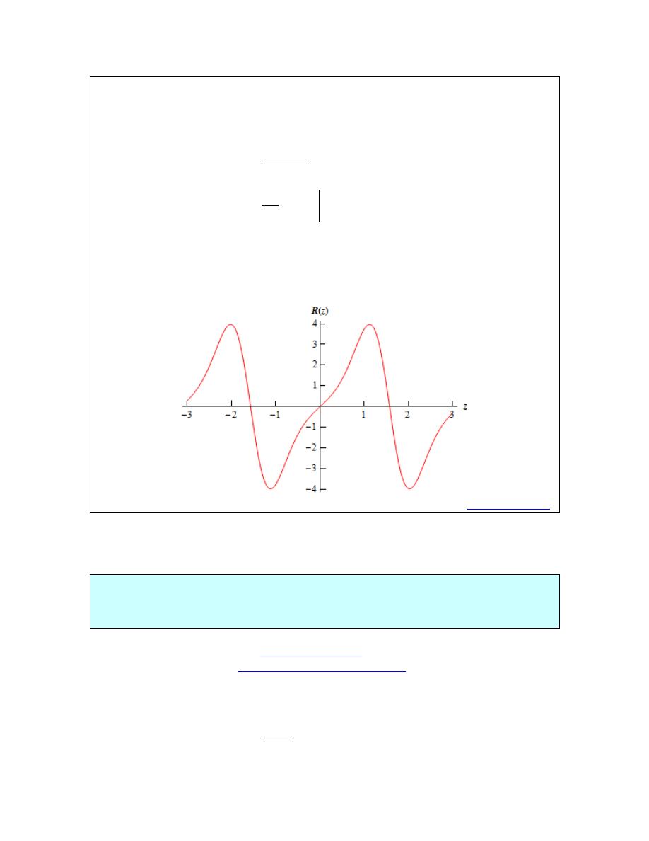
(b)
( )
( )
( )
1 cos 2
sin 2
z
R z
z
−
=
e
on
[
]
,
π π
−
Again, not much to do here other than use the formula. Note that the integral will need the
© 2007 Paul Dawkins
4
http://tutorial.math.lamar.edu/terms.aspx
Calculus I
following substitution.
( )
1 cos 2
u
z
= −
Here is the average value of this function,
( )
( )
( )
( )
1 cos 2
1 cos 2
1
sin 2
1
4
0
z
avg
z
R
z
dz
π
π
π
π
π
π
π
−
−
−
−
=
− −
=
=
∫
e
e
So, in this case the average function value is zero. Do not get excited about getting zero here. It
will happen on occasion. In fact, if you look at the graph of the function on this interval it’s not
too hard to see that this is the correct answer.
[
Return to Problems
]
There is also a theorem that is related to the average function value.
The Mean Value Theorem for Integrals
If
( )
f x
is a continuous function on [a,b] then there is a number c in [a,b] such that,
( )
( )(
)
b
a
f x dx
f c b a
=
−
∫
Note that this is very similar to the
Mean Value Theorem
that we saw in the Derivatives
Applications chapter. See the
Proof of Various Integral Properties
section of the Extras chapter
for the proof.
Note that one way to think of this theorem is the following. First rewrite the result as,
( )
( )
1
b
a
f x dx
f c
b a
=
−
∫
© 2007 Paul Dawkins
5
http://tutorial.math.lamar.edu/terms.aspx
Calculus I
and from this we can see that this theorem is telling us that there is a number
a
c
b
< <
such that
( )
avg
f
f c
=
. Or, in other words, if
( )
f x
is a continuous function then somewhere in [a,b] the
function will take on its average value.
Let’s take a quick look at an example using this theorem.
Example 2
Determine the number c that satisfies the Mean Value Theorem for Integrals for the
function
( )
2
3
2
f x
x
x
=
+
+
on the interval [1,4]
Solution
First let’s notice that the function is a polynomial and so is continuous on the given interval. This
means that we can use the Mean Value Theorem. So, let’s do that.
(
)
(
)
(
)
4
2
2
1
4
3
2
2
1
2
2
3
2
3
2 4 1
1
3
2
3
3
2
3
2
99
3
9
6
2
7
0
3
9
2
x
x
dx
c
c
x
x
x
c
c
c
c
c
c
+
+
=
+
+
−
+
+
=
+
+
=
+
+
8
=
+
−
∫
This is a quadratic equation that we can solve. Using the quadratic formula we get the following
two solutions,
3
67
2.593
2
3
67
5.593
2
c
c
− +
=
=
− −
=
= −
Clearly the second number is not in the interval and so that isn’t the one that we’re after. The
first however is in the interval and so that’s the number we want.
Note that it is possible for both numbers to be in the interval so don’t expect only one to be in the
interval.
© 2007 Paul Dawkins
6
http://tutorial.math.lamar.edu/terms.aspx
Calculus I
Area Between Curves
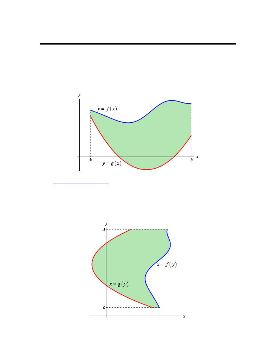
In this section we are going to look at finding the area between two curves. There are actually
two cases that we are going to be looking at.
In the first case we want to determine the area between
( )
y
f x
=
and
( )
y
g x
=
on the interval
[a,b]. We are also going to assume that
( )
( )
f x
g x
≥
. Take a look at the following sketch to
get an idea of what we’re initially going to look at.
In the
Area and Volume Formulas
section of the Extras chapter we derived the following formula
for the area in this case.
( ) ( )
b
a
A
f x
g x dx
=
−
∫
(1)
The second case is almost identical to the first case. Here we are going to determine the area
between
( )
x
f y
=
and
( )
x
g y
=
on the interval [c,d] with
( )
( )
f y
g y
≥
.
© 2007 Paul Dawkins
7
http://tutorial.math.lamar.edu/terms.aspx
Calculus I
In this case the formula is,
( ) ( )
d
c
A
f y
g y dy
=
−
∫
(2)
Now (1) and (2) are perfectly serviceable formulas, however, it is sometimes easy to forget that
these always require the first function to be the larger of the two functions. So, instead of these
formulas we will instead use the following “word” formulas to make sure that we remember that
the area is always the “larger” function minus the “smaller” function.
In the first case we will use,
upper
lower
,
function
function
b
a
A
dx
a
x
b
=
−
≤ ≤
⌠
⌡
(3)
In the second case we will use,
right
left
,
function
function
d
c
A
dy
c
y
d
=
−
≤ ≤
⌠
⌡
(4)
Using these formulas will always force us to think about what is going on with each problem and
to make sure that we’ve got the correct order of functions when we go to use the formula.
Let’s work an example.
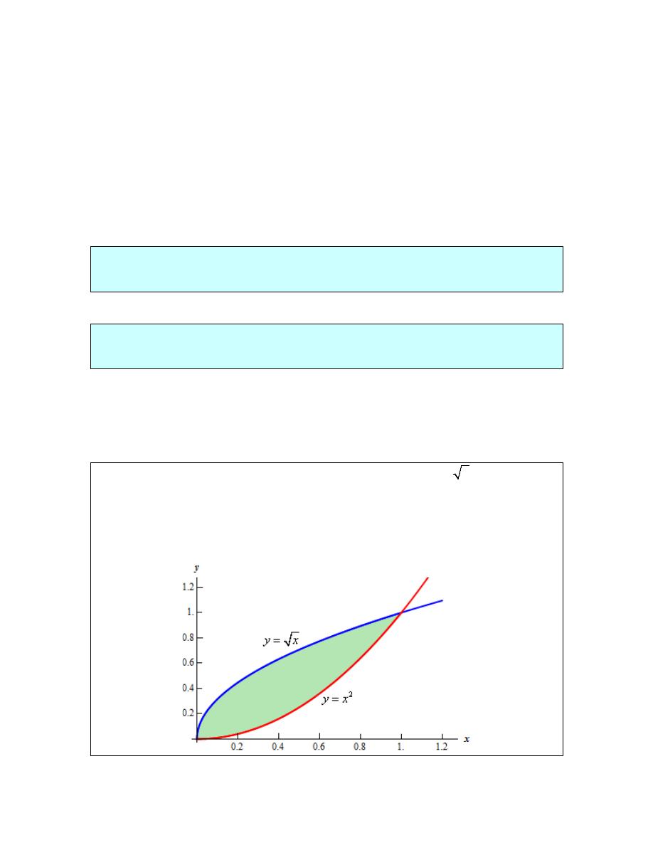
Example 1
Determine the area of the region enclosed by
2
y
x
=
and
y
x
=
.
Solution
First of all, just what do we mean by “area enclosed by”. This means that the region we’re
interested in must have one of the two curves on every boundary of the region. So, here is a
graph of the two functions with the enclosed region shaded.
© 2007 Paul Dawkins
8
http://tutorial.math.lamar.edu/terms.aspx
Calculus I
Note that we don’t take any part of the region to the right of the intersection point of these two
graphs. In this region there is no boundary on the right side and so is not part of the enclosed
area. Remember that one of the given functions must be on the each boundary of the enclosed
region.
Also from this graph it’s clear that the upper function will be dependent on the range of x’s that
we use. Because of this you should always sketch of a graph of the region. Without a sketch it’s
often easy to mistake which of the two functions is the larger. In this case most would probably
say that
2
y
x
=
is the upper function and they would be right for the vast majority of the x’s.
However, in this case it is the lower of the two functions.
The limits of integration for this will be the intersection points of the two curves. In this case it’s
pretty easy to see that they will intersect at
0
x
=
and
1
x
=
so these are the limits of integration.
So, the integral that we’ll need to compute to find the area is,
1
2
0
1
3
3
2
0
upper
lower
function
function
2
1
3
3
1
3
b
a
A
dx
x
x dx
x
x
=
−
=
−
=
−
=
⌠
⌡
∫
Before moving on to the next example, there are a couple of important things to note.
First, in almost all of these problems a graph is pretty much required. Often the bounding region,
which will give the limits of integration, is difficult to determine without a graph.
Also, it can often be difficult to determine which of the functions is the upper function and which
is the lower function without a graph. This is especially true in cases like the last example where
the answer to that question actually depended upon the range of x’s that we were using.
Finally, unlike the area under a curve that we looked at in the previous chapter the area between
two curves will always be positive. If we get a negative number or zero we can be sure that
we’ve made a mistake somewhere and will need to go back and find it.
Note as well that sometimes instead of saying region enclosed by we will say region bounded by.
They mean the same thing.
Let’s work some more examples.
© 2007 Paul Dawkins
9
http://tutorial.math.lamar.edu/terms.aspx
Calculus I
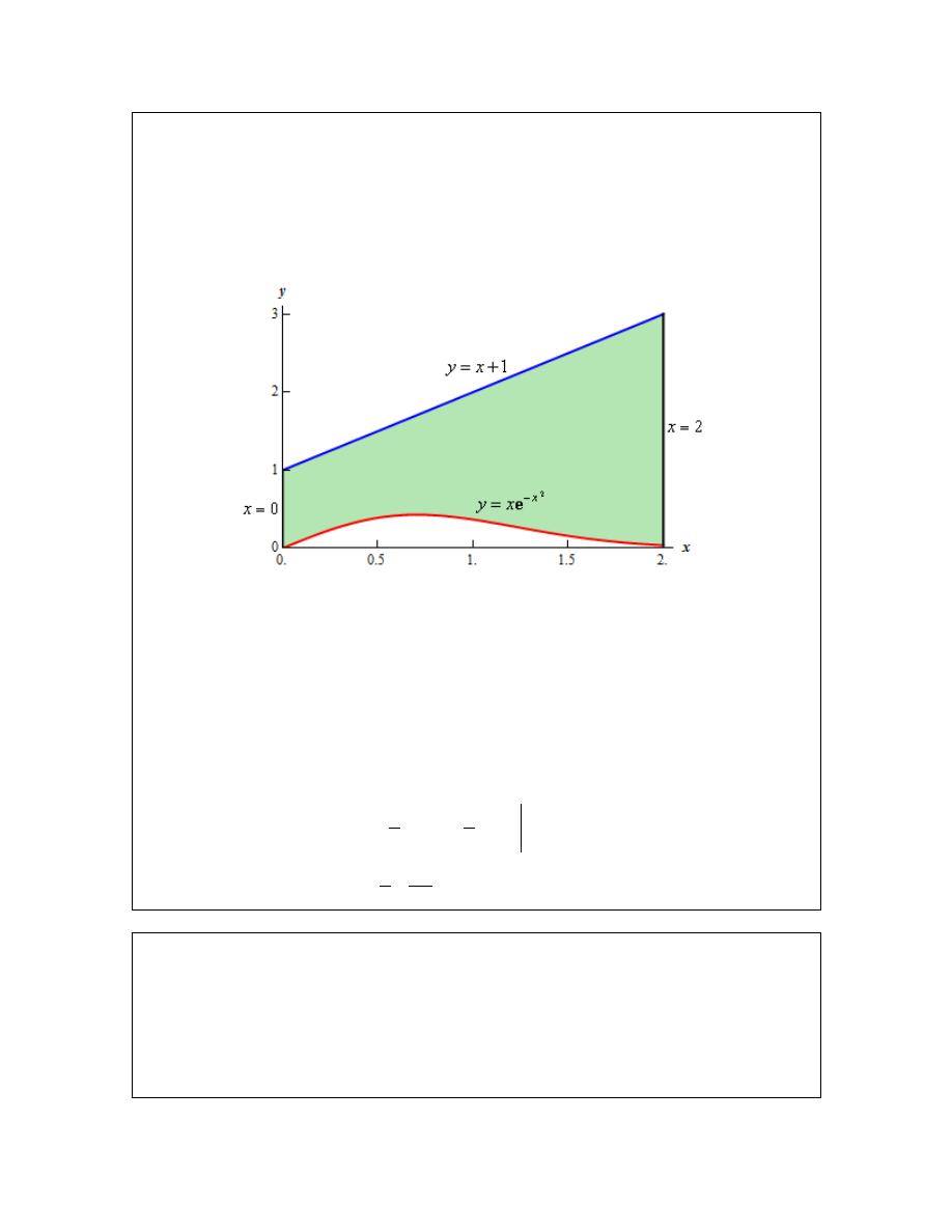
Example 2
Determine the area of the region bounded by
2
x
y
x
−
= e
,
1
y
x
= +
,
2
x
=
, and the
y-axis.
Solution
In this case the last two pieces of information,
2
x
=
and the y-axis, tell us the right and left
boundaries of the region. Also, recall that the y-axis is given by the line
0
x
=
. Here is the graph
with the enclosed region shaded in.
Here, unlike the first example, the two curves don’t meet. Instead we rely on two vertical lines to
bound the left and right sides of the region as we noted above
Here is the integral that will give the area.
2
0
2
2
0
4
2
2
upper
lower
function
function
1
1
1
2
2
7
3.5092
2
2
b
a
x
x
A
dx
x
x
dx
x
x
−
−
−
=
−
=
+ −
=
+ +
= +
=
⌠
⌡
∫
e
e
e
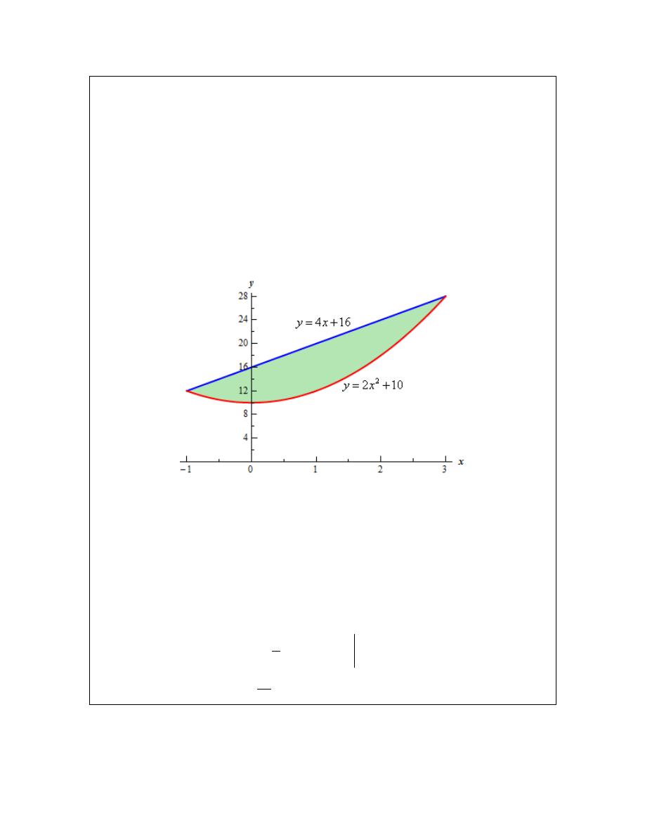
Example 3
Determine the area of the region bounded by
2
2
10
y
x
=
+
and
4
16
y
x
=
+
.
Solution
In this case the intersection points (which we’ll need eventually) are not going to be easily
identified from the graph so let’s go ahead and get them now. Note that for most of these
problems you’ll not be able to accurately identify the intersection points from the graph and so
you’ll need to be able to determine them by hand. In this case we can get the intersection points
© 2007 Paul Dawkins
10
http://tutorial.math.lamar.edu/terms.aspx
Calculus I
by setting the two equations equal.
(
)(
)
2
2
2
10
4
16
2
4
6
0
2
1
3
0
x
x
x
x
x
x
+
=
+
−
− =
+
− =
So it looks like the two curves will intersect at
1
x
= −
and
3
x
=
. If we need them we can get
the y values corresponding to each of these by plugging the values back into either of the
equations. We’ll leave it to you to verify that the coordinates of the two intersection points on the
graph are (-1,12) and (3,28).
Note as well that if you aren’t good at graphing knowing the intersection points can help in at
least getting the graph started. Here is a graph of the region.
With the graph we can now identify the upper and lower function and so we can now find the
enclosed area.
(
)
3
2
1
3
2
1
3
3
2
1
upper
lower
function
function
4
16
2
10
2
4
6
2
2
6
3
64
3
b
a
A
dx
x
x
dx
x
x
dx
x
x
x
−
−
−
=
−
=
+
−
+
=
−
+
+
= −
+
+
=
⌠
⌡
∫
∫
Be careful with parenthesis in these problems. One of the more common mistakes students make
with these problems is to neglect parenthesis on the second term.
© 2007 Paul Dawkins
11
http://tutorial.math.lamar.edu/terms.aspx
Calculus I
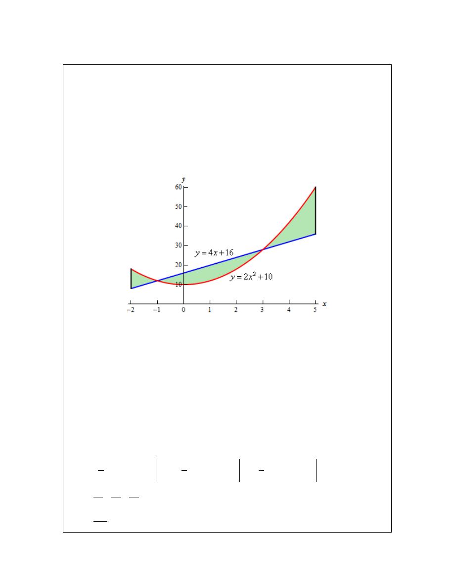
Example 4
Determine the area of the region bounded by
2
2
10
y
x
=
+
,
4
16
y
x
=
+
,
2
x
= −
and
5
x
=
Solution
So, the functions used in this problem are identical to the functions from the first problem. The
difference is that we’ve extended the bounded region out from the intersection points. Since
these are the same functions we used in the previous example we won’t bother finding the
intersection points again.
Here is a graph of this region.
Okay, we have a small problem here. Our formula requires that one function always be the upper
function and the other function always be the lower function and we clearly do not have that here.
However, this actually isn’t the problem that it might at first appear to be. There are three regions
in which one function is always the upper function and the other is always the lower function.
So, all that we need to do is find the area of each of the three regions, which we can do, and then
add them all up.
Here is the area.
(
)
(
)
(
)
1
3
5
2
2
2
2
1
3
1
3
5
2
2
2
2
1
3
1
3
5
3
2
3
2
3
2
2
1
3
2
10
4
16
4
16
2
10
2
10
4
16
2
4
6
2
4
6
2
4
6
2
2
2
2
6
2
6
2
6
3
3
3
14
64
64
3
3
3
142
3
A
x
x
dx
x
x
dx
x
x
dx
x
x
dx
x
x
dx
x
x
dx
x
x
x
x
x
x
x
x
x
−
−
−
−
−
−
−
−
−
=
+
−
+
+
+
−
+
+
+
−
+
=
−
−
+
−
+
+
+
−
−
=
−
−
+ −
+
+
+
−
−
=
+
+
=
∫
∫
∫
∫
∫
∫
© 2007 Paul Dawkins
12
http://tutorial.math.lamar.edu/terms.aspx
Calculus I
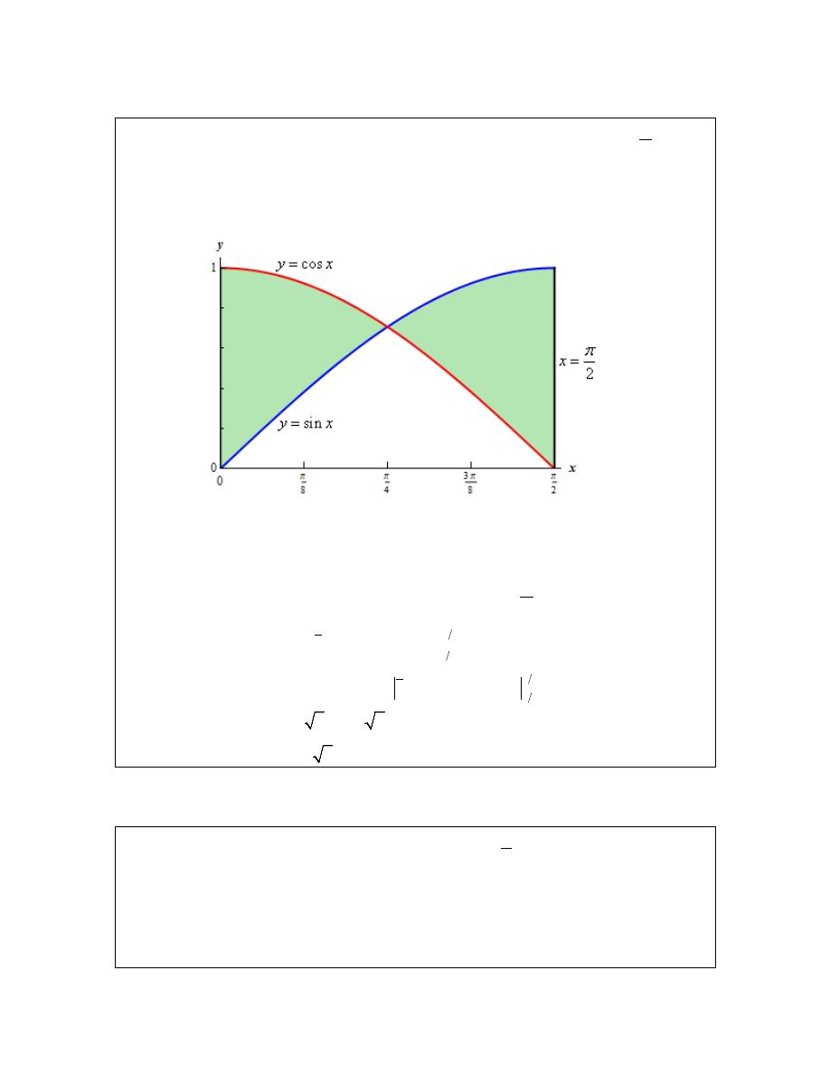
Example 5
Determine the area of the region enclosed by
sin
y
x
=
,
cos
y
x
=
,
2
x
π
=
, and the
y-axis.
Solution
First let’s get a graph of the region.
So, we have another situation where we will need to do two integrals to get the area. The
intersection point will be where
sin
cos
x
x
=
in the interval. We’ll leave it to you to verify that this will be
4
x
π
=
. The area is then,
(
)
(
)
(
)
2
4
0
4
2
4
0
4
cos
sin
sin
cos
sin
cos
cos
sin
2 1
2 1
2 2
2
0.828427
A
x
x dx
x
x dx
x
x
x
x
π
π
π
π
π
π
=
−
+
−
=
+
+ −
−
=
− +
−
=
− =
∫
∫
We will need to be careful with this next example.
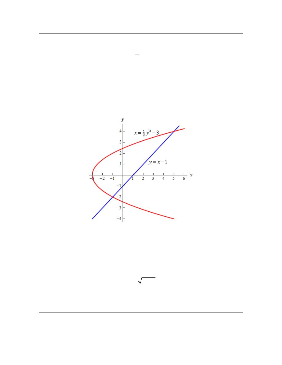
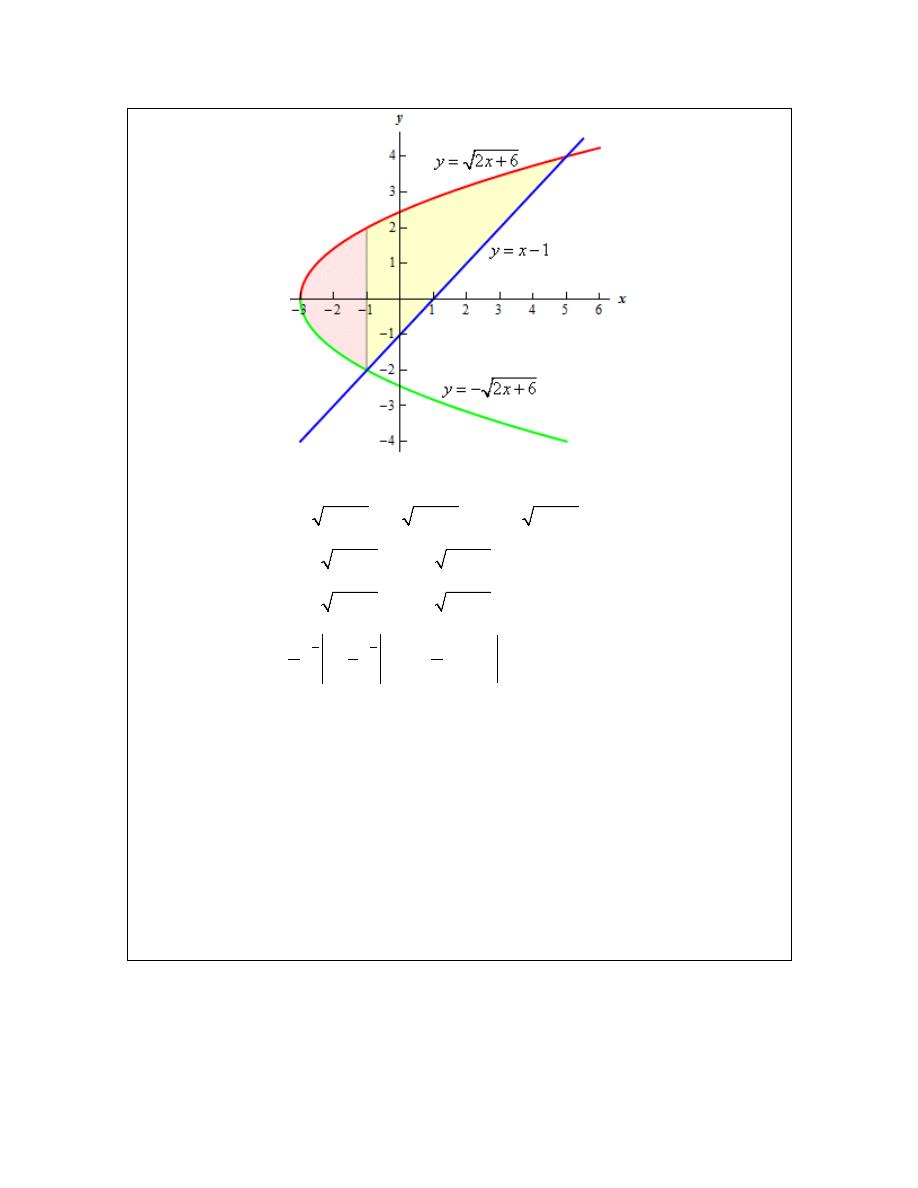
Example 6
Determine the area of the region enclosed by
2
1
3
2
x
y
=
−
and
1
y
x
= −
.
Solution
Don’t let the first equation get you upset. We will have to deal with these kinds of equations
occasionally so we’ll need to get used to dealing with them.
As always, it will help if we have the intersection points for the two curves. In this case we’ll get
© 2007 Paul Dawkins
13
http://tutorial.math.lamar.edu/terms.aspx
Calculus I
the intersection points by solving the second equation for x and then setting them equal. Here is
that work,
(
)(
)
2
2
2
1
1
3
2
2
2
6
0
2
8
0
4
2
y
y
y
y
y
y
y
y
+ =
−
+ =
−
=
−
−
=
−
+
So, it looks like the two curves will intersect at
2
y
= −
and
4
y
=
or if we need the full
coordinates they will be : (-1,-2) and (5,4).
Here is a sketch of the two curves.
Now, we will have a serious problem at this point if we aren’t careful. To this point we’ve been
using an upper function and a lower function. To do that here notice that there are actually two
portions of the region that will have different lower functions. In the range [-2,-1] the parabola is
actually both the upper and the lower function.
To use the formula that we’ve been using to this point we need to solve the parabola for y. This
gives,
2
6
y
x
= ±
+
where the “+” gives the upper portion of the parabola and the “-” gives the lower portion.
Here is a sketch of the complete area with each region shaded that we’d need if we were going to
use the first formula.
© 2007 Paul Dawkins
14
http://tutorial.math.lamar.edu/terms.aspx
Calculus I
The integrals for the area would then be,
(
)
(
)
1
5
3
1
1
5
3
1
1
5
5
3
1
1
4
16
5
3
3
2
2
2
1
0
4
2
6
2
6
2
6
1
2 2
6
2
6
1
2 2
6
2
6
1
2
1
1
3
3
2
18
A
x
x
dx
x
x
dx
x
dx
x
x
dx
x
dx
x
dx
x
dx
u
u
x
x
−
−
−
−
−
−
−
−
−
−
−
=
+ − −
+
+
+ − −
=
+
+
+ − +
=
+
+
+
+
− +
=
+
+ −
+
=
∫
∫
∫
∫
∫
∫
∫
While these integrals aren’t terribly difficult they are more difficult than they need to be.
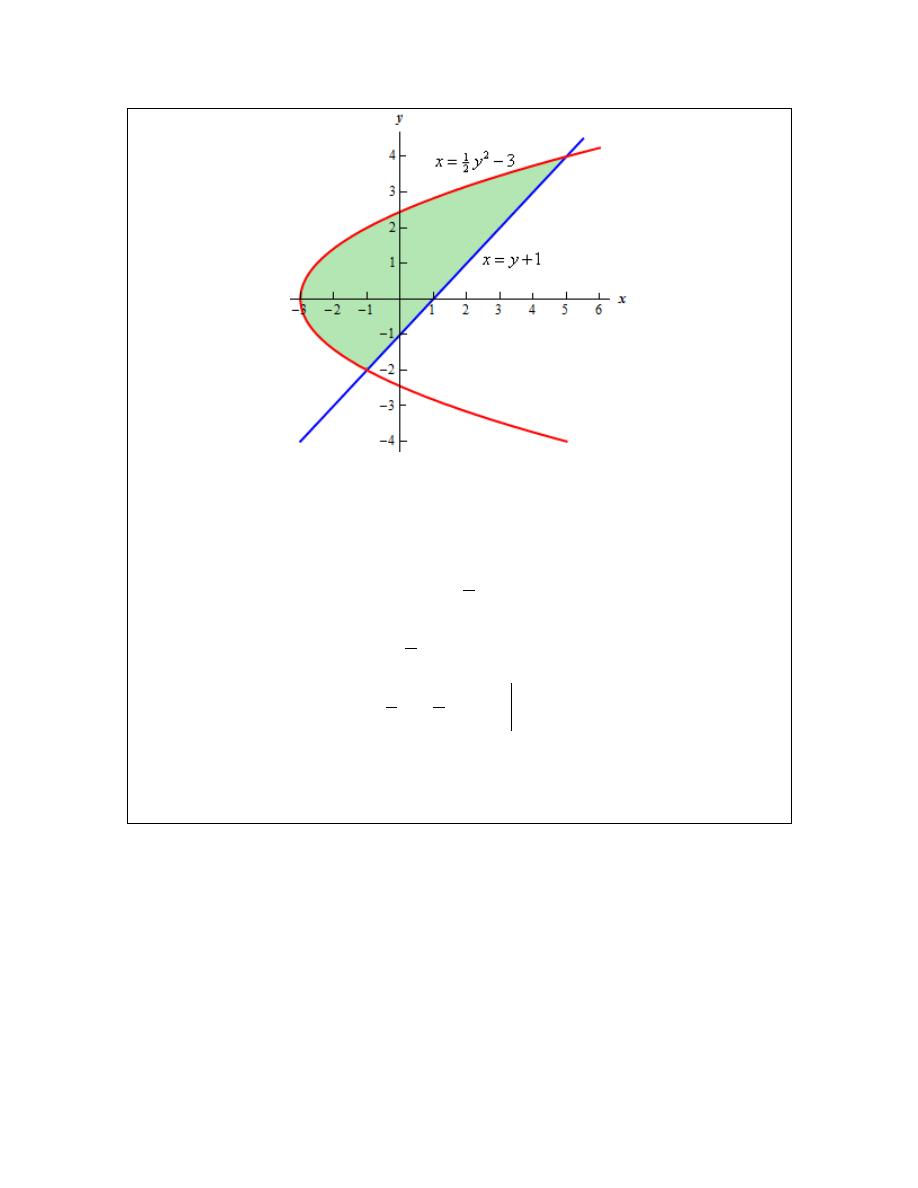
Recall that there is another formula for determining the area. It is,
right
left
,
function
function
d
c
A
dy
c
y
d
=
−
≤ ≤
⌠
⌡
and in our case we do have one function that is always on the left and the other is always on the
right. So, in this case this is definitely the way to go. Note that we will need to rewrite the
equation of the line since it will need to be in the form
( )
x
f y
=
but that is easy enough to do.
Here is the graph for using this formula.
© 2007 Paul Dawkins
15
http://tutorial.math.lamar.edu/terms.aspx
Calculus I
The area is,
(
)
4
2
2
4
2
2
4
3
2
2
right
left
function
function
1
1
3
2
1
4
2
1
1
4
6
2
18
d
c
A
dy
y
y
dy
y
y
dy
y
y
y
−
−
−
=
−
=
+ −
−
=
−
+ +
= −
+
+
=
⌠
⌡
⌠
⌡
⌠
⌡
This is the same that we got using the first formula and this was definitely easier than the first
method.
So, in this last example we’ve seen a case where we could use either formula to find the area.
However, the second was definitely easier.
Students often come into a calculus class with the idea that the only easy way to work with
functions is to use them in the form
( )
y
f x
=
. However, as we’ve seen in this previous
example there are definitely times when it will be easier to work with functions in the form
( )
x
f y
=
. In fact, there are going to be occasions when this will be the only way in which a
problem can be worked so make sure that you can deal with functions in this form.
© 2007 Paul Dawkins
16
http://tutorial.math.lamar.edu/terms.aspx
Calculus I
Let’s take a look at one more example to make sure we can deal with functions in this form.
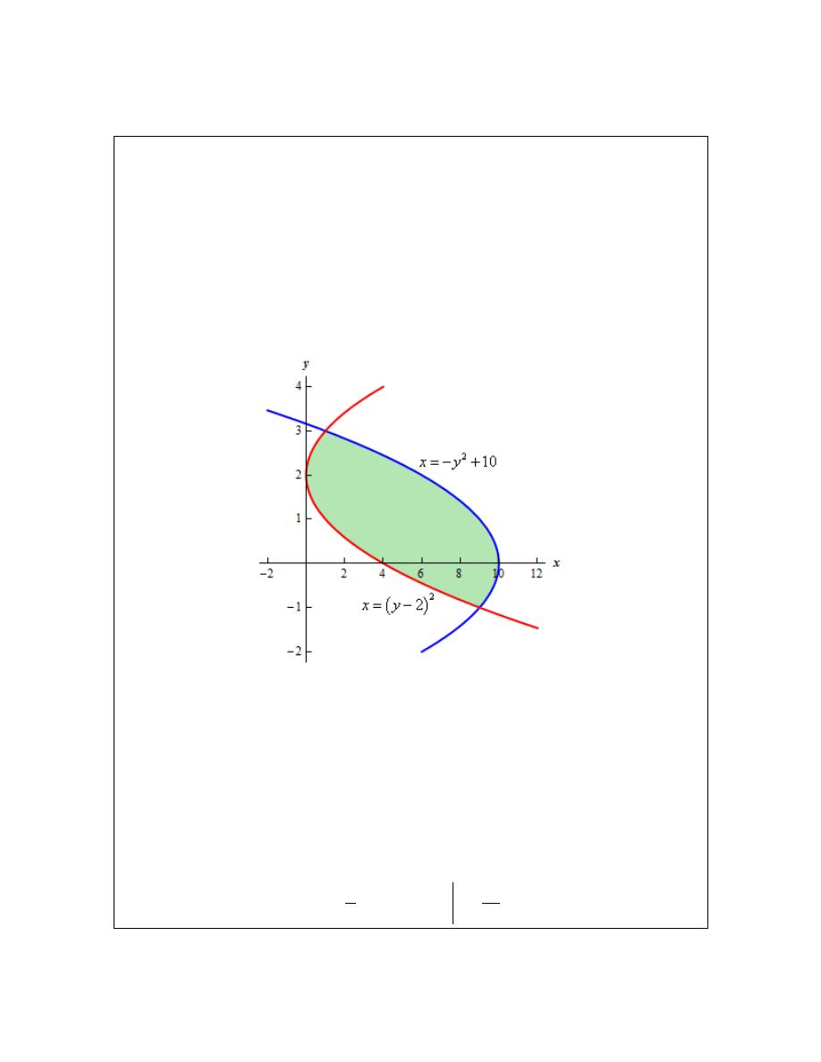
Example 7
Determine the area of the region bounded by
2
10
x
y
= − +
and
(
)
2
2
x
y
=
−
.
Solution
First, we will need intersection points.
(
)
(
)(
)
2
2
2
2
2
10
2
10
4
4
0
2
4
6
0
2
1
3
y
y
y
y
y
y
y
y
y
− +
=
−
− +
=
−
+
=
−
−
=
+
−
The intersection points are
1
y
= −
and
3
y
=
. Here is a sketch of the region.
This is definitely a region where the second area formula will be easier. If we used the first
formula there would be three different regions that we’d have to look at.
The area in this case is,
(
)
3
2
2
1
3
2
1
3
3
2
1
right
left
function
function
10
2
2
4
6
2
4
2
6
3
3
d
c
A
dy
y
y
dy
y
y
dy
y
y
y
−
−
−
=
−
=
− +
−
−
=
−
+
+
6
= −
+
+
=
⌠
⌡
∫
∫
© 2007 Paul Dawkins
17
http://tutorial.math.lamar.edu/terms.aspx
Calculus I
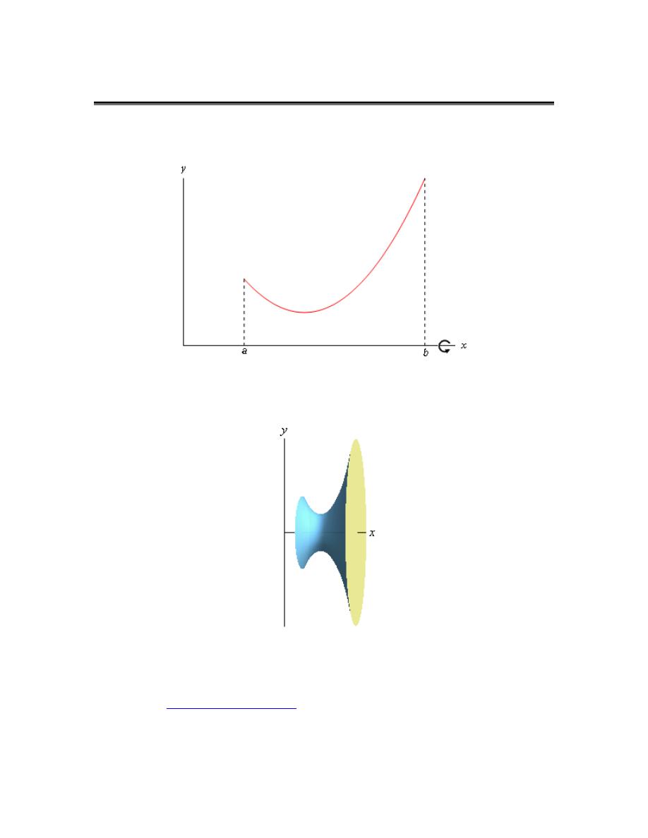
Volumes of Solids of Revolution / Method of Rings
In this section we will start looking at the volume of a solid of revolution. We should first define
just what a solid of revolution is. To get a solid of revolution we start out with a function,
( )
y
f x
=
, on an interval [a,b].
We then rotate this curve about a given axis to get the surface of the solid of revolution. For
purposes of this discussion let’s rotate the curve about the x-axis, although it could be any vertical
or horizontal axis. Doing this for the curve above gives the following three dimensional region.
What we want to do over the course of the next two sections is to determine the volume of this
object.
In the final the
Area and Volume Formulas
section of the Extras chapter we derived the following
formulas for the volume of this solid.
© 2007 Paul Dawkins
18
http://tutorial.math.lamar.edu/terms.aspx

Calculus I
( )
( )
b
d
a
c
V
A x dx
V
A y dy
=
=
∫
∫
where,
( )
A x
and
( )
A y
is the cross-sectional area of the solid. There are many ways to get the
cross-sectional area and we’ll see two (or three depending on how you look at it) over the next
two sections. Whether we will use
( )
A x
or
( )
A y
will depend upon the method and the axis of
rotation used for each problem.
One of the easier methods for getting the cross-sectional area is to cut the object perpendicular to
the axis of rotation. Doing this the cross section will be either a solid disk if the object is solid (as
our above example is) or a ring if we’ve hollowed out a portion of the solid (we will see this
eventually).
In the case that we get a solid disk the area is,
(
)
2
radius
A
π
=
where the radius will depend upon the function and the axis of rotation.
In the case that we get a ring the area is,
2
2
outer
inner
radius
radius
A
π
=
−
where again both of the radii will depend on the functions given and the axis of rotation. Note as
well that in the case of a solid disk we can think of the inner radius as zero and we’ll arrive at the
correct formula for a solid disk and so this is a much more general formula to use.
Also, in both cases, whether the area is a function of x or a function of y will depend upon the
axis of rotation as we will see.
This method is often called the method of disks or the method of rings.
Let’s do an example.
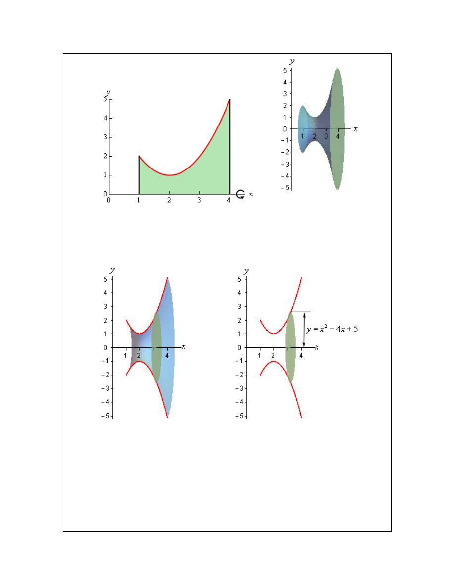
Example 1
Determine the volume of the solid obtained by rotating the region bounded by
2
4
5
y
x
x
=
−
+
,
1
x
=
,
4
x
=
, and the x-axis about the x-axis.
Solution
The first thing to do is get a sketch of the bounding region and the solid obtained by rotating the
region about the x-axis. Here are both of these sketches.
© 2007 Paul Dawkins
19
http://tutorial.math.lamar.edu/terms.aspx
Calculus I
Okay, to get a cross section we cut the solid at any x. Below are a couple of sketches showing a
typical cross section. The sketch on the right shows a cut away of the object with a typical cross
section without the caps. The sketch on the left shows just the curve we’re rotating as well as its
mirror image along the bottom of the solid.
In this case the radius is simply the distance from the x-axis to the curve and this is nothing more
than the function value at that particular x as shown above. The cross-sectional area is then,
( )
(
)
(
)
2
2
4
3
2
4
5
8
26
40
25
A x
x
x
x
x
x
x
π
π
=
−
+
=
−
+
−
+
Next we need to determine the limits of integration. Working from left to right the first cross
section will occur at
1
x
=
and the last cross section will occur at
4
x
=
. These are the limits of
integration.
© 2007 Paul Dawkins
20
http://tutorial.math.lamar.edu/terms.aspx
Calculus I
The volume of this solid is then,
( )
4
4
3
2
1
4
5
4
3
2
1
8
26
40
25
1
26
2
20
25
5
3
78
5
b
a
V
A x dx
x
x
x
x
dx
x
x
x
x
x
π
π
π
=
=
−
+
−
+
=
−
+
−
+
=
∫
∫
In the above example the object was a solid object, but the more interesting objects are those that
are not solid so let’s take a look at one of those.
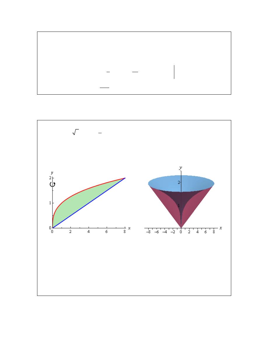
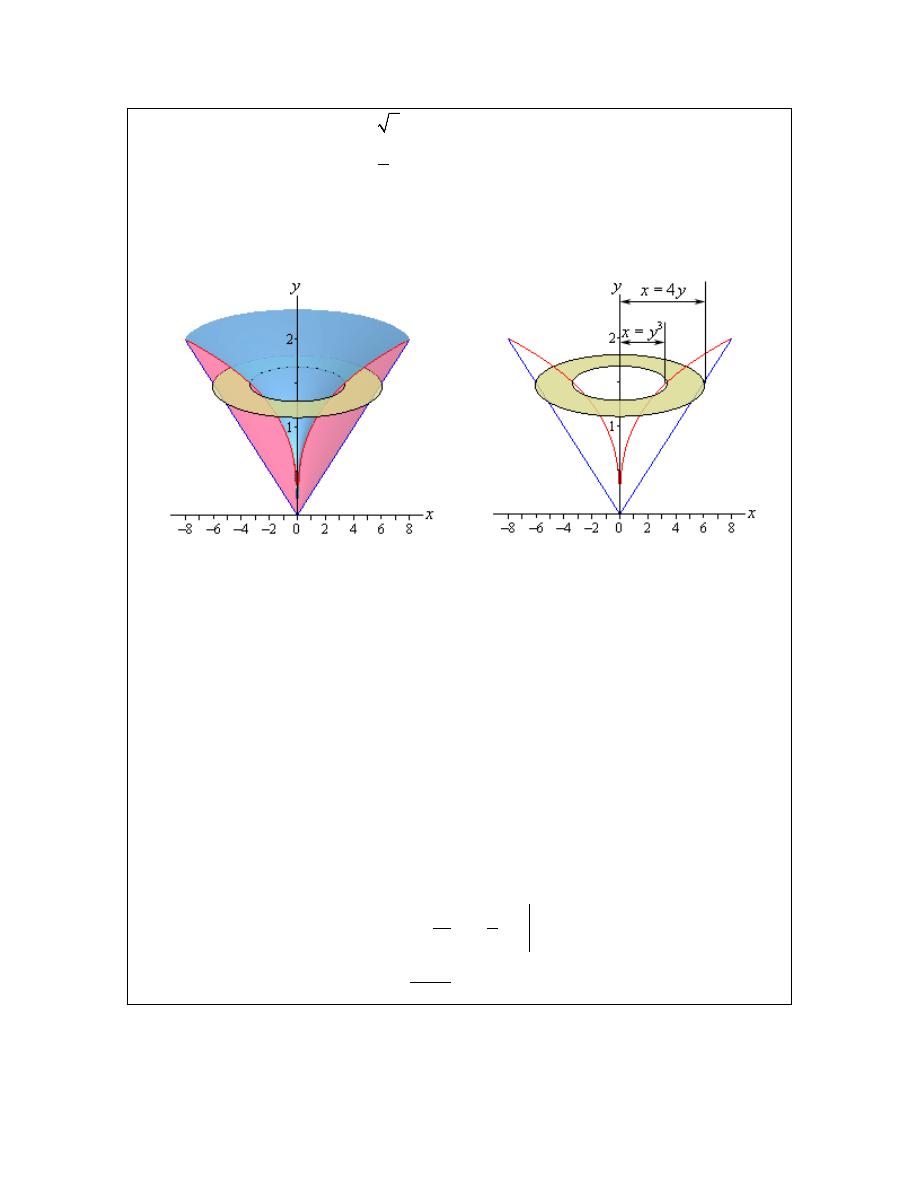
Example 2
Determine the volume of the solid obtained by rotating the portion of the region
bounded by
3
y
x
=
and
4
x
y
=
that lies in the first quadrant about the y-axis.
Solution
First, let’s get a graph of the bounding region and a graph of the object. Remember that we only
want the portion of the bounding region that lies in the first quadrant. There is a portion of the
bounding region that is in the third quadrant as well, but we don't want that for this problem.
There are a couple of things to note with this problem. First, we are only looking for the volume
of the “walls” of this solid, not the complete interior as we did in the last example.
Next, we will get our cross section by cutting the object perpendicular to the axis of rotation. The
cross section will be a ring (remember we are only looking at the walls) for this example and it
will be horizontal at some y. This means that the inner and outer radius for the ring will be x
values and so we will need to rewrite our functions into the form
( )
x
f y
=
. Here are the
functions written in the correct form for this example.
© 2007 Paul Dawkins
21
http://tutorial.math.lamar.edu/terms.aspx
Calculus I
3
3
4
4
y
x
x
y
x
y
x
y
=
⇒
=
=
⇒
=
Here are a couple of sketches of the boundaries of the walls of this object as well as a typical ring.
The sketch on the left includes the back portion of the object to give a little context to the figure
on the right.
The inner radius in this case is the distance from the y-axis to the inner curve while the outer
radius is the distance from the y-axis to the outer curve. Both of these are then x distances and so
are given by the equations of the curves as shown above.
The cross-sectional area is then,
( )
( )
( )
(
)
(
)
2
2
3
2
6
4
16
A y
y
y
y
y
π
π
=
−
=
−
Working from the bottom of the solid to the top we can see that the first cross-section will occur
at
0
y
=
and the last cross-section will occur at
2
y
=
. These will be the limits of integration.
The volume is then,
( )
2
2
6
0
2
3
7
0
16
16
1
3
7
512
21
d
c
V
A y dy
y
y dy
y
y
π
π
π
=
=
−
=
−
=
∫
∫
With these two examples out of the way we can now make a generalization about this method. If
we rotate about a horizontal axis (the x-axis for example) then the cross sectional area will be a
© 2007 Paul Dawkins
22
http://tutorial.math.lamar.edu/terms.aspx
Calculus I
function of x. Likewise, if we rotate about a vertical axis (the y-axis for example) then the cross
sectional area will be a function of y.
The remaining two examples in this section will make sure that we don’t get too used to the idea
of always rotating about the x or y-axis.
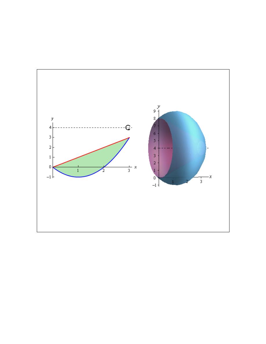
Example 3
Determine the volume of the solid obtained by rotating the region bounded by
2
2
y
x
x
=
−
and
y
x
=
about the line
4
y
=
.
Solution
First let’s get the bounding region and the solid graphed.
Again, we are going to be looking for the volume of the walls of this object. Also since we are
rotating about a horizontal axis we know that the cross-sectional area will be a function of x.
Here are a couple of sketches of the boundaries of the walls of this object as well as a typical ring.
The sketch on the left includes the back portion of the object to give a little context to the figure
on the right.
© 2007 Paul Dawkins
23
http://tutorial.math.lamar.edu/terms.aspx
Calculus I
Now, we’re going to have to be careful here in determining the inner and outer radius as they
aren’t going to be quite as simple they were in the previous two examples.
Let’s start with the inner radius as this one is a little clearer. First, the inner radius is NOT x. The
distance from the x-axis to the inner edge of the ring is x, but we want the radius and that is the
distance from the axis of rotation to the inner edge of the ring. So, we know that the distance
from the axis of rotation to the x-axis is 4 and the distance from the x-axis to the inner ring is x.
The inner radius must then be the difference between these two. Or,
inner radius
4
x
= −
The outer radius works the same way. The outer radius is,
(
)
2
2
outer radius
4
2
2
4
x
x
x
x
= −
−
= − +
+
Note that given the location of the typical ring in the sketch above the formula for the outer radius
may not look quite right but it is in fact correct. As sketched the outer edge of the ring is below
the x-axis and at this point the value of the function will be negative and so when we do the
subtraction in the formula for the outer radius we’ll actually be subtracting off a negative number
which has the net effect of adding this distance onto 4 and that gives the correct outer radius.
Likewise, if the outer edge is above the x-axis, the function value will be positive and so we’ll be
doing an honest subtraction here and again we’ll get the correct radius in this case.
The cross-sectional area for this case is,
( )
(
)
(
)
(
)
(
)
2
2
2
4
3
2
2
4
4
4
5
24
A x
x
x
x
x
x
x
x
π
π
=
− +
+
− −
=
−
−
+
© 2007 Paul Dawkins
24
http://tutorial.math.lamar.edu/terms.aspx
Calculus I
The first ring will occur at
0
x
=
and the last ring will occur at
3
x
=
and so these are our limits
of integration. The volume is then,
( )
3
4
3
2
0
3
5
4
3
2
0
4
5
24
1
5
12
5
3
153
5
b
a
V
A x dx
x
x
x
x dx
x
x
x
x
π
π
π
=
=
−
−
+
=
−
−
+
=
∫
∫
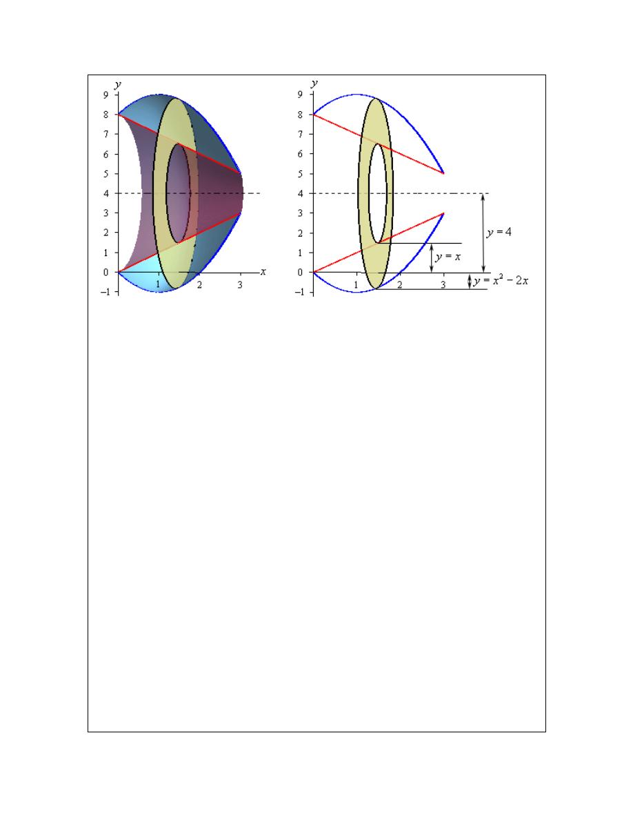
Example 4
Determine the volume of the solid obtained by rotating the region bounded by
2
1
y
x
=
−
and
1
y
x
= −
about the line
1
x
= −
.
Solution
As with the previous examples, let’s first graph the bounded region and the solid.
Now, let’s notice that since we are rotating about a vertical axis and so the cross-sectional area
will be a function of y. This also means that we are going to have to rewrite the functions to also
get them in terms of y.
2
2
1
1
4
1
1
y
y
x
x
y
x
x
y
=
−
⇒
=
+
= −
⇒
= +
Here are a couple of sketches of the boundaries of the walls of this object as well as a typical ring.
The sketch on the left includes the back portion of the object to give a little context to the figure
on the right.
© 2007 Paul Dawkins
25
http://tutorial.math.lamar.edu/terms.aspx
Calculus I
The inner and outer radius for this case is both similar and different from the previous example.
This example is similar in the sense that the radii are not just the functions. In this example the
functions are the distances from the y-axis to the edges of the rings. The center of the ring
however is a distance of 1 from the y-axis. This means that the distance from the center to the
edges is a distance from the axis of rotation to the y-axis (a distance of 1) and then from the y-axis
to the edge of the rings.
So, the radii are then the functions plus 1 and that is what makes this example different from the
previous example. Here we had to add the distance to the function value whereas in the previous
example we needed to subtract the function from this distance. Note that without sketches the
radii on these problems can be difficult to get.
So, in summary, we’ve got the following for the inner and outer radius for this example.
2
2
outer radius
1 1
2
inner radius
1 1
2
4
4
y
y
y
y
= + + = +
=
+ + =
+
The cross-sectional area is then,
( )
(
)
2
2
4
2
2
2
4
4
16
y
y
A y
y
y
π
π
=
+
−
+
=
−
The first ring will occur at
0
y
=
and the final ring will occur at
4
y
=
and so these will be our
limits of integration.
The volume is,
© 2007 Paul Dawkins
26
http://tutorial.math.lamar.edu/terms.aspx
Calculus I
( )
4
4
0
4
2
5
0
4
16
1
2
80
96
5
d
c
V
A y dy
y
y
dy
y
y
π
π
π
=
=
−
=
−
=
⌠
⌡
∫
© 2007 Paul Dawkins
27
http://tutorial.math.lamar.edu/terms.aspx
Calculus I
Volumes of Solids of Revolution / Method of Cylinders
In the previous section we started looking at finding volumes of solids of revolution. In that
section we took cross sections that were rings or disks, found the cross-sectional area and then
used the following formulas to find the volume of the solid.
( )
( )
b
d
a
c
V
A x dx
V
A y dy
=
=
∫
∫
In the previous section we only used cross sections that were in the shape of a disk or a ring. This
however does not always need to be the case. We can use any shape for the cross sections as long
as it can be expanded or contracted to completely cover the solid we’re looking at. This is a good
thing because as our first example will show us we can’t always use rings/disks.
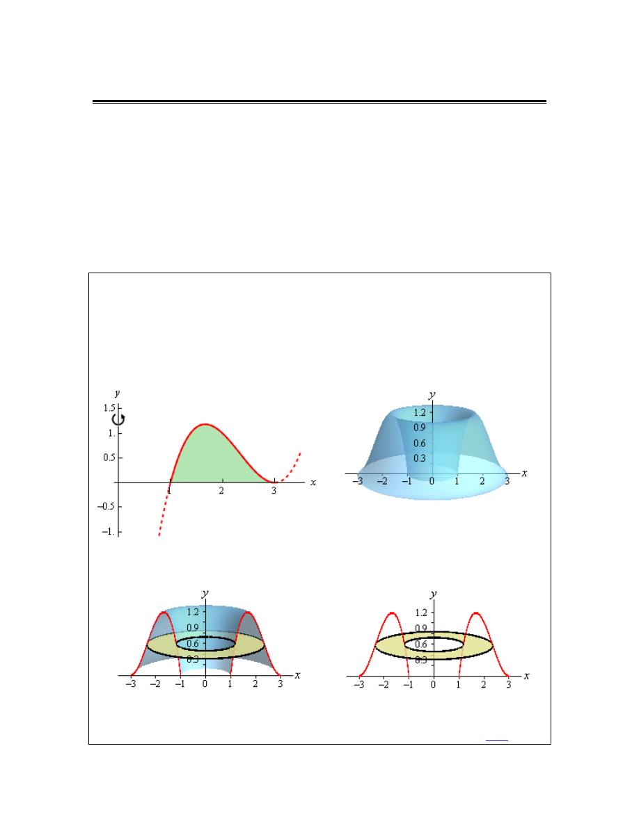
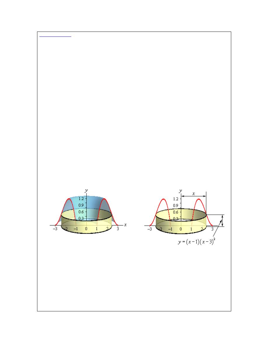
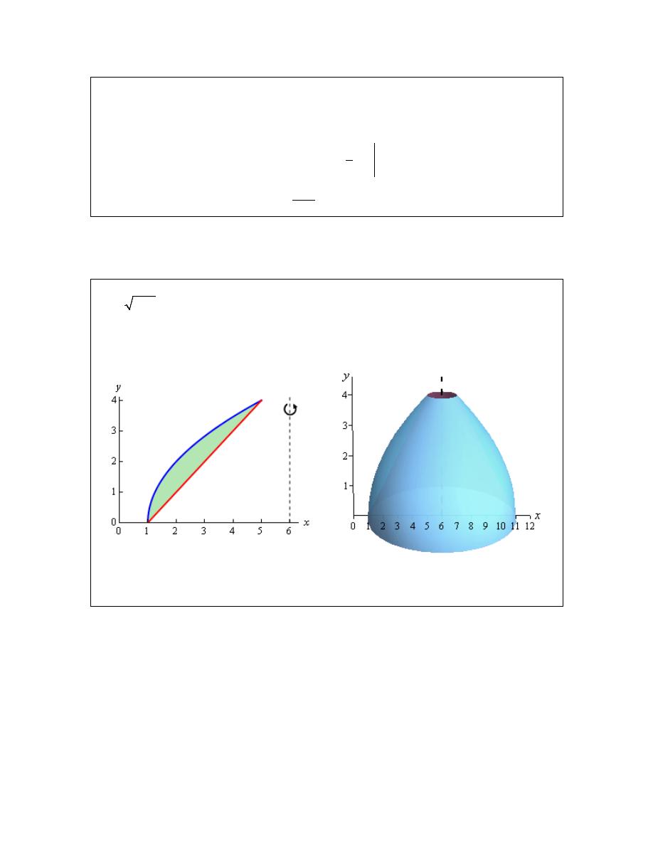
Example 1
Determine the volume of the solid obtained by rotating the region bounded by
(
)(
)
2
1
3
y
x
x
=
−
−
and the x-axis about the y-axis.
Solution
As we did in the previous section, let’s first graph the bounded region and solid. Note that the
bounded region here is the shaded portion shown. The curve is extended out a little past this for
the purposes of illustrating what the curve looks like.
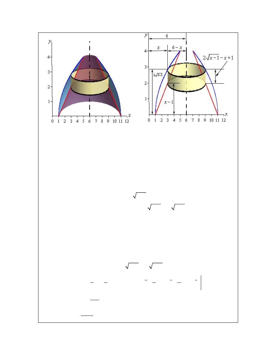
So, we’ve basically got something that’s roughly doughnut shaped. If we were to use rings on
this solid here is what a typical ring would look like.
This leads to several problems. First, both the inner and outer radius are defined by the same
function. This, in itself, can be dealt with on occasion as we saw in a example in the
Area
© 2007 Paul Dawkins
28
http://tutorial.math.lamar.edu/terms.aspx
Calculus I
Between Curves
section. However, this usually means more work than other methods so it’s
often not the best approach.
This leads to the second problem we got here. In order to use rings we would need to put this
function into the form
( )
x
f y
=
. That is NOT easy in general for a cubic polynomial and in
other cases may not even be possible to do. Even when it is possible to do this the resulting
equation is often significantly messier than the original which can also cause problems.
The last problem with rings in this case is not so much a problem as it’s just added work. If we
were to use rings the limit would be y limits and this means that we will need to know how high
the graph goes. To this point the limits of integration have always been intersection points that
were fairly easy to find. However, in this case the highest point is not an intersection point, but
instead a relative maximum. We spent several sections in the Applications of Derivatives
chapter talking about how to find maximum values of functions. However, finding them can, on
occasion, take some work.
So, we’ve seen three problems with rings in this case that will either increase our work load or
outright prevent us from using rings.
What we need to do is to find a different way to cut the solid that will give us a cross-sectional
area that we can work with. One way to do this is to think of our solid as a lump of cookie dough
and instead of cutting it perpendicular to the axis of rotation we could instead center a cylindrical
cookie cutter on the axis of rotation and push this down into the solid. Doing this would give the
following picture,
Doing this gives us a cylinder or shell in the object and we can easily find its surface area. The
surface area of this cylinder is,
( )
(
)(
)
( ) (
)(
)
(
)
(
)
2
4
3
2
2
radius
height
2
1
3
2
7
15
9
A x
x
x
x
x
x
x
x
π
π
π
=
=
−
−
=
−
+
−
Notice as well that as we increase the radius of the cylinder we will completely cover the solid
and so we can use this in our formula to find the volume of this solid. All we need are limits of
integration. The first cylinder will cut into the solid at
1
x
=
and as we increase x to
3
x
=
we
© 2007 Paul Dawkins
29
http://tutorial.math.lamar.edu/terms.aspx
Calculus I
will completely cover both sides of the solid since expanding the cylinder in one direction will
automatically expand it in the other direction as well.
The volume of this solid is then,
( )
3
4
3
2
1
3
5
4
3
2
1
2
7
15
9
1
7
9
2
5
5
4
2
24
5
b
a
V
A x dx
x
x
x
x dx
x
x
x
x
π
π
π
=
=
−
+
−
=
−
+
−
=
∫
∫
The method used in the last example is called the method of cylinders or method of shells. The
formula for the area in all cases will be,
(
)(
)
2
radius
height
A
π
=
There are a couple of important differences between this method and the method of rings/disks
that we should note before moving on. First, rotation about a vertical axis will give an area that is
a function of x and rotation about a horizontal axis will give an area that is a function of y. This is
exactly opposite of the method of rings/disks.
Second, we don’t take the complete range of x or y for the limits of integration as we did in the
previous section. Instead we take a range of x or y that will cover one side of the solid. As we
noted in the first example if we expand out the radius to cover one side we will automatically
expand in the other direction as well to cover the other side.
Let’s take a look at another example.
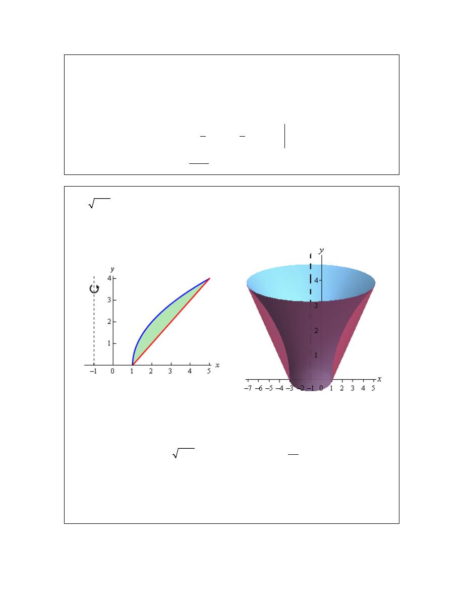
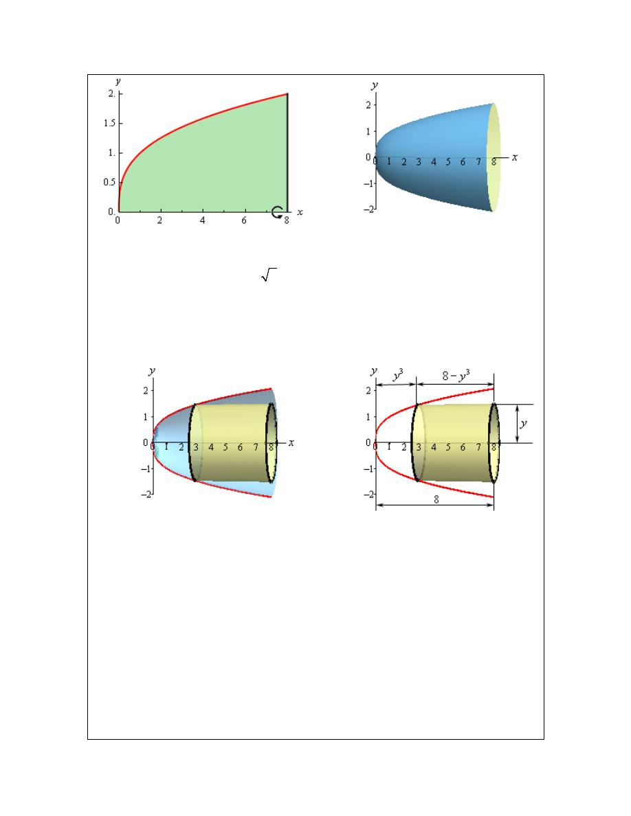
Example 2
Determine the volume of the solid obtained by rotating the region bounded by
3
y
x
=
,
8
x
=
and the x-axis about the x-axis.
Solution
First let’s get a graph of the bounded region and the solid.
© 2007 Paul Dawkins
30
http://tutorial.math.lamar.edu/terms.aspx
Calculus I
Okay, we are rotating about a horizontal axis. This means that the area will be a function of y and
so our equation will also need to be written in
( )
x
f y
=
form.
3
3
y
x
x
y
=
⇒
=
As we did in the ring/disk section let’s take a couple of looks at a typical cylinder. The sketch on
the left shows a typical cylinder with the back half of the object also in the sketch to give the right
sketch some context. The sketch on the right contains a typical cylinder and only the curves that
define the edge of the solid.
In this case the width of the cylinder is not the function value as it was in the previous example.
In this case the function value is the distance between the edge of the cylinder and the y-axis. The
distance from the edge out to the line is
8
x
=
and so the width is then
3
8
y
−
. The cross
sectional area in this case is,
( )
(
)(
)
( )
(
)
(
)
3
4
2
radius
width
2
8
2
8
A y
y
y
y
y
π
π
π
=
=
−
=
−
The first cylinder will cut into the solid at
0
y
=
and the final cylinder will cut in at
2
y
=
and so
these are our limits of integration.
The volume of this solid is,
© 2007 Paul Dawkins
31
http://tutorial.math.lamar.edu/terms.aspx
Calculus I
( )
2
4
0
2
2
5
0
2
8
1
2
4
5
96
5
d
c
V
A y dy
y
y dy
y
y
π
π
π
=
=
−
=
−
=
∫
∫
The remaining examples in this section will have axis of rotation about axis other than the x and
y-axis. As with the method of rings/disks we will need to be a little careful with these.
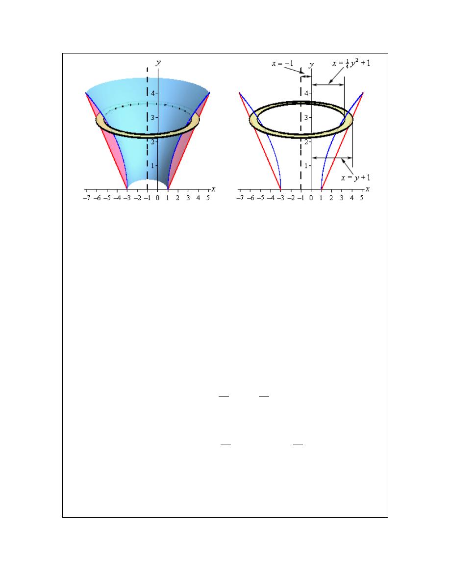
Example 3
Determine the volume of the solid obtained by rotating the region bounded by
2
1
y
x
=
−
and
1
y
x
= −
about the line
6
x
=
.
Solution
Here’s a graph of the bounded region and solid.
Here are our sketches of a typical cylinder. Again, the sketch on the left is here to provide some
context for the sketch on the right.
© 2007 Paul Dawkins
32
http://tutorial.math.lamar.edu/terms.aspx
Calculus I
Okay, there is a lot going on in the sketch to the left. First notice that the radius is not just an x or
y as it was in the previous two cases. In this case x is the distance from the y-axis to the edge of
the cylinder and we need the distance from the axis of rotation to the edge of the cylinder. That
means that the radius of this cylinder is
6
x
−
.
Secondly, the height of the cylinder is the difference of the two functions in this case.
The cross sectional area is then,
( )
(
)(
)
(
)
(
)
(
)
2
2
radius
height
2
6
2
1
1
2
7
6 12
1 2
1
A x
x
x
x
x
x
x
x x
π
π
π
=
=
−
− − +
=
−
+ +
− −
−
Now the first cylinder will cut into the solid at
1
x
=
and the final cylinder will cut into the solid
at
5
x
=
so there are our limits.
Here is the volume.
( )
(
)
(
)
(
)
5
2
1
5
3
3
5
3
2
2
2
2
1
2
7
6 12
1 2
1
1
7
4
4
2
6
8
1
1
1
3
2
3
5
136
2
15
272
15
b
a
V
A x dx
x
x
x
x x
dx
x
x
x
x
x
x
π
π
π
π
=
=
−
+ +
− −
−
=
−
+
+
−
−
−
−
−
=
=
∫
∫
© 2007 Paul Dawkins
33
http://tutorial.math.lamar.edu/terms.aspx
Calculus I
The integration of the last term is a little tricky so let’s do that here. It will use the substitution,
1
1
u
x
du
dx
x
u
= −
=
= +
(
)
(
)
(
)
1
2
3
1
2
2
5
3
2
2
5
3
2
2
2
1
2
1
2
2
2
2
5
3
4
4
1
1
5
3
x x
dx
u
u du
u
u du
u
u
c
x
x
c
−
=
+
=
+
=
+
+
=
−
+
−
+
⌠
⌡
∫
∫
We saw one of these kinds of substitutions back in the
substitution
section.
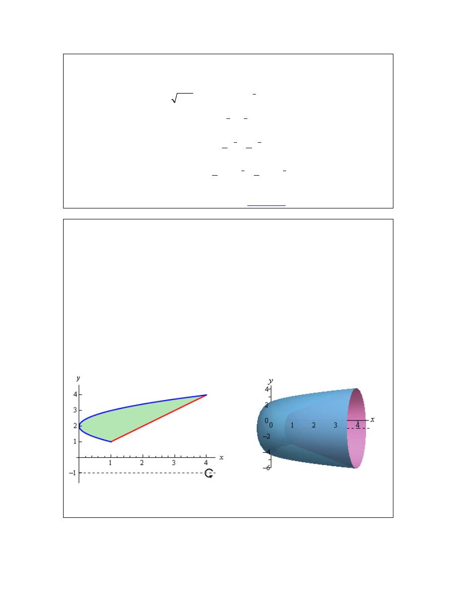
Example 4
Determine the volume of the solid obtained by rotating the region bounded by
(
)
2
2
x
y
=
−
and
y
x
=
about the line
1
y
= −
.
Solution
We should first get the intersection points there.
(
)
(
)(
)
2
2
2
2
4
4
0
5
4
0
4
1
y
y
y
y
y
y
y
y
y
=
−
=
−
+
=
−
+
=
−
−
So, the two curves will intersect at
1
y
=
and
4
y
=
. Here is a sketch of the bounded region and
the solid.
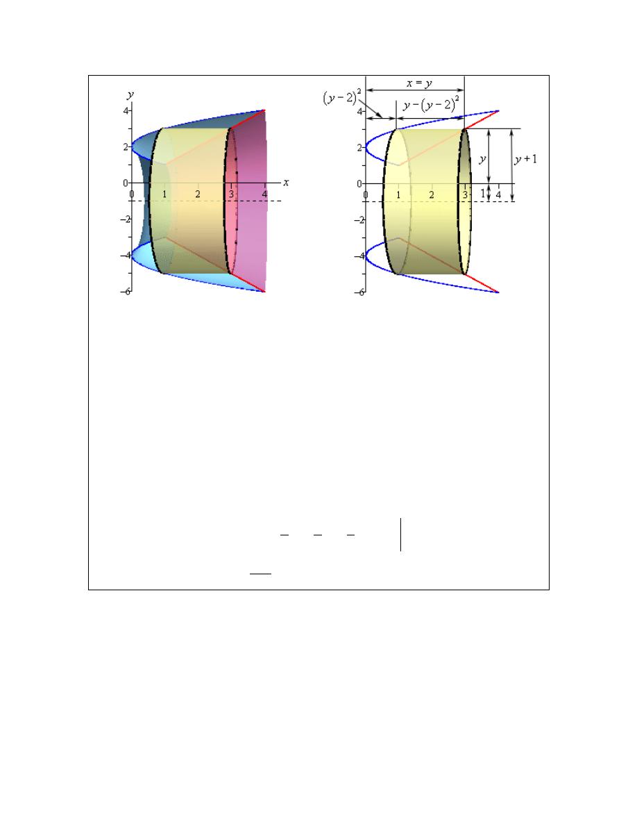
Here are our sketches of a typical cylinder. The sketch on the left is here to provide some context
for the sketch on the right.
© 2007 Paul Dawkins
34
http://tutorial.math.lamar.edu/terms.aspx
Calculus I
Here’s the cross sectional area for this cylinder.
( )
(
)(
)
(
)
(
)
(
)
(
)
2
3
2
2
radius
width
2
1
2
2
4
4
A y
y
y
y
y
y
y
π
π
π
=
=
+
−
−
=
− +
+ −
The first cylinder will cut into the solid at
1
y
=
and the final cylinder will cut in at
4
y
=
. The
volume is then,
( )
4
3
2
1
4
4
3
2
1
2
4
4
1
4
1
2
4
4
3
2
63
2
d
c
V
A y dy
y
y
y
dy
y
y
y
y
π
π
π
=
=
− +
+ −
=
−
+
+
−
=
∫
∫
© 2007 Paul Dawkins
35
http://tutorial.math.lamar.edu/terms.aspx
Calculus I
More Volume Problems
In this section we’re going to take a look at some more volume problems. However, the
problems we’ll be looking at here will not be solids of revolution as we looked at in the previous
two sections. There are many solids out there that cannot be generated as solids of revolution, or
at least not easily and so we need to take a look at how to do some of these problems.
Now, having said that these will not be solids of revolutions they will still be worked in pretty
much the same manner. For each solid we’ll need to determine the cross-sectional area, either
( )
A x
or
( )
A y
, and they use the formulas we used in the previous two sections,
( )
( )
b
d
a
c
V
A x dx
V
A y dy
=
=
∫
∫
The “hard” part of these problems will be determining what the cross-sectional area for each solid
is. Each problem will be different and so each cross-sectional area will be determined by
different means.
Also, before we proceed with any examples we need to acknowledge that the integrals in this
section might look a little tricky at first. There are going to be very few numbers in these
problems. All of the examples in this section are going to be more general derivation of volume
formulas for certain solids. As such we’ll be working with things like circles of radius r and
we’ll not be giving a specific value of r and we’ll have heights of h instead of specific heights,
etc.
All the letters in the integrals are going to make the integrals look a little tricky, but all you have
to remember is that the r’s and the h’s are just letters being used to represent a fixed quantity for
the problem, i.e. it is a constant. So when we integrate we only need to worry about the letter in
the differential as that is the variable we’re actually integrating with respect to. All other letters
in the integral should be thought of as constants. If you have trouble doing that, just think about
what you’d do if the r was a 2 or the h was a 3 for example.
Let’s start with a simple example that we don’t actually need to do an integral that will illustrate
how these problems work in general and will get us used to seeing multiple letters in integrals.
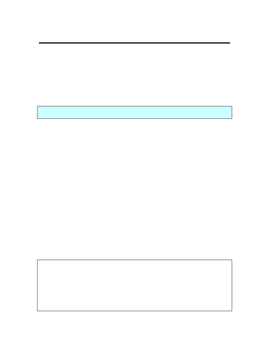
Example 1
Find the volume of a cylinder of radius r and height h.
Solution
Now, as we mentioned before starting this example we really don’t need to use an integral to find
this volume, but it is a good example to illustrate the method we’ll need to use for these types of
problems.
We’ll start off with the sketch of the cylinder below.
© 2007 Paul Dawkins
36
http://tutorial.math.lamar.edu/terms.aspx
Calculus I
We’ll center the cylinder on the x-axis and the cylinder will start at
0
x
=
and end at
x
h
=
as
shown. Note that we’re only choosing this particular set up to get an integral in terms of x and to
make the limits nice to deal with. There are many other orientations that we could use.
What we need here is to get a formula for the cross-sectional area at any x. In this case the cross-
sectional area is constant and will be a disk of radius r. Therefore, for any x we’ll have the
following cross-sectional area,
( )
2
A x
r
π
=
Next the limits for the integral will be
0
x
h
≤ ≤
since that is the range of x in which the cylinder
lives. Here is the integral for the volume,
2
2
2
2
0
0
0
h
h
h
V
r dx
r
dx
r x
r h
π
π
π
π
=
=
=
=
∫
∫
So, we get the expected formula.
Also, recall we are using r to represent the radius of the cylinder. While r can clearly take
different values it will never change once we start the problem. Cylinders do not change their
radius in the middle of a problem and so as we move along the center of the cylinder (i.e. the x-
axis) r is a fixed number and won’t change. In other words it is a constant that will not change as
we change the x. Therefore, because we integrated with respect to x the r will be a constant as far
as the integral is concerned. The r can then be pulled out of the integral as shown (although that’s
not required, we just did it to make the point). At this point we’re just integrating dx and we
know how to do that.
When we evaluate the integral remember that the limits are x values and so we plug into the x and
NOT the r. Again, remember that r is just a letter that is being used to represent the radius of the
cylinder and, once we start the integration, is assumed to be a fixed constant.
As noted before we started this example if you’re having trouble with the r just think of what
you’d do if there was a 2 there instead of an r. In this problem, because we’re integrating with
respect to x, both the 2 and the r will behave in the same manner. Note however that you should
NEVER actually replace the r with a 2 as that WILL lead to a wrong answer. You should just
think of what you would do IF the r was a 2.
© 2007 Paul Dawkins
37
http://tutorial.math.lamar.edu/terms.aspx
Calculus I
So, to work these problems we’ll first need to get a sketch of the solid with a set of x and y axes to
help us see what’s going on. At the very least we’ll need the sketch to get the limits of the
integral, but we will often need it to see just what the cross-sectional area is. Once we have the
sketch we’ll need to determine a formula for the cross-sectional area and then do the integral.
Let’s work a couple of more complicated examples. In these examples the main issue is going to
be determining what the cross-sectional areas are.
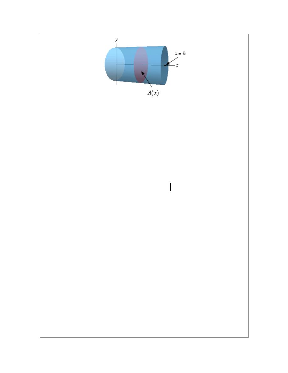
Example 2
Find the volume of a pyramid whose base is a square with sides of length L and
whose height is h.
Solution
Let’s start off with a sketch of the pyramid. In this case we’ll center the pyramid on the y-axis
and to make the equations easier we are going to position the point of the pyramid at the origin.
Now, as shown here the cross-sectional area will be a function of y and it will also be a square
with sides of length s. The area of the square is easy, but we’ll need to get the length of the side
in terms of y. To determine this consider the figure on the right above. If we look at the pyramid
directly from the front we’ll see that we have two similar triangles and we know that the ratio of
any two sides of similar triangles must be equal. In other words, we know that,
s
y
y
L
s
L
y
L
h
h
h
=
⇒
=
=
So, the cross-sectional area is then,
( )
2
2
2
2
L
A y
s
y
h
=
=
© 2007 Paul Dawkins
38
http://tutorial.math.lamar.edu/terms.aspx
Calculus I
The limit for the integral will be
0
y
h
≤ ≤
and the volume will be,
2
2
2
2
2
3
2
2
2
2
0
0
0
1
1
3
3
h
h
h
L
L
L
V
y dy
y dy
y
L h
h
h
h
=
=
=
=
⌠
⌡
∫
Again, do not get excited about the L and the h in the integral. Once we start the problem if we
change y they will not change and so they are constants as far as the integral is concerned and can
get pulled out of the integral. Also, remember that when we evaluate will only plug the limits
into the variable we integrated with respect to, y in this case.
Before we proceed with some more complicated examples we should once again remind you to
not get excited about the other letters in the integrals. If we’re integrating with respect to x or y
then all other letters in the formula that represent fixed quantities (i.e. radius, height, length of a
side, etc.) are just constants and can be treated as such when doing the integral.
Now let’s do some more examples.
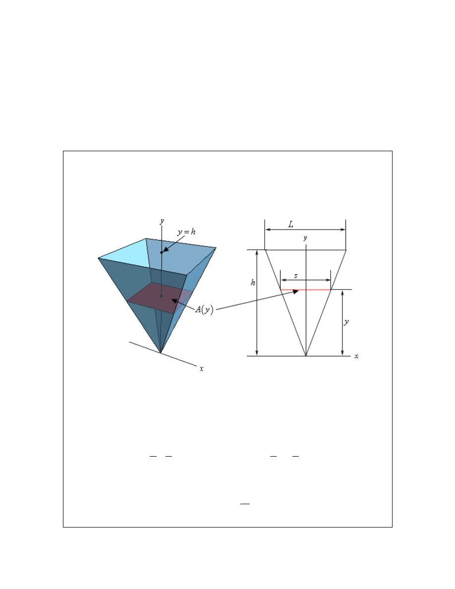
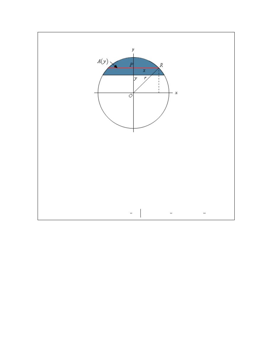
Example 3
For a sphere of radius r find the volume of the cap of height h.
Solution
A sketch is probably best to illustrate what we’re after here.
We are after the top portion of the sphere and the height of this is portion is h. In this case we’ll
use a cross-sectional area that starts at the bottom of the cap, which is at
y
r
h
= −
, and moves up
towards the top, which is at
y
r
=
. So, each cross-section will be a disk of radius x. It is a little
easier to see that the radius will be x if we look at it from the top as shown in the sketch to the
right above. The area of this disk is then,
2
x
π
This is a problem however as we need the cross-sectional area in terms of y. So, what we really
© 2007 Paul Dawkins
39
http://tutorial.math.lamar.edu/terms.aspx
Calculus I
need to determine what
2
x
will be for any given y at the cross-section. To get this let’s look at
the sphere from the front.
In particular look at the triangle POR. Because the point R lies on the sphere itself we can see
that the length of the hypotenuse of this triangle (the line OR) is r, the radius of the sphere. The
line PR has a length of x and the line OP has length y so by the Pythagorean Theorem we know,
2
2
2
2
2
2
x
y
r
x
r
y
+
=
⇒
=
−
So, we now know what
2
x
will be for any given y and so the cross-sectional area is,
( )
(
)
2
2
A y
r
y
π
=
−
As we noted earlier the limits on y will be
r
h
y
r
− ≤ ≤
and so the volume is,
(
)
(
)
(
)
(
)
2
2
2
3
2
3
2
1
1
1
3
3
3
r
r
r h
r h
V
r
y
dy
r y
y
h r
h
h
r
h
π
π
π
π
−
−
=
−
=
−
=
−
=
−
∫
In the previous example we again saw an r in the integral. However, unlike the previous two
examples it was not multiplied times the x or the y and so could not be pulled out of the integral.
In this case it was like we were integrating
2
4
y
−
and we know how integrate that. So, in this
case we need to treat the
2
r
like the 4 and so when we integrate that we’ll pick up a y.
© 2007 Paul Dawkins
40
http://tutorial.math.lamar.edu/terms.aspx
Calculus I
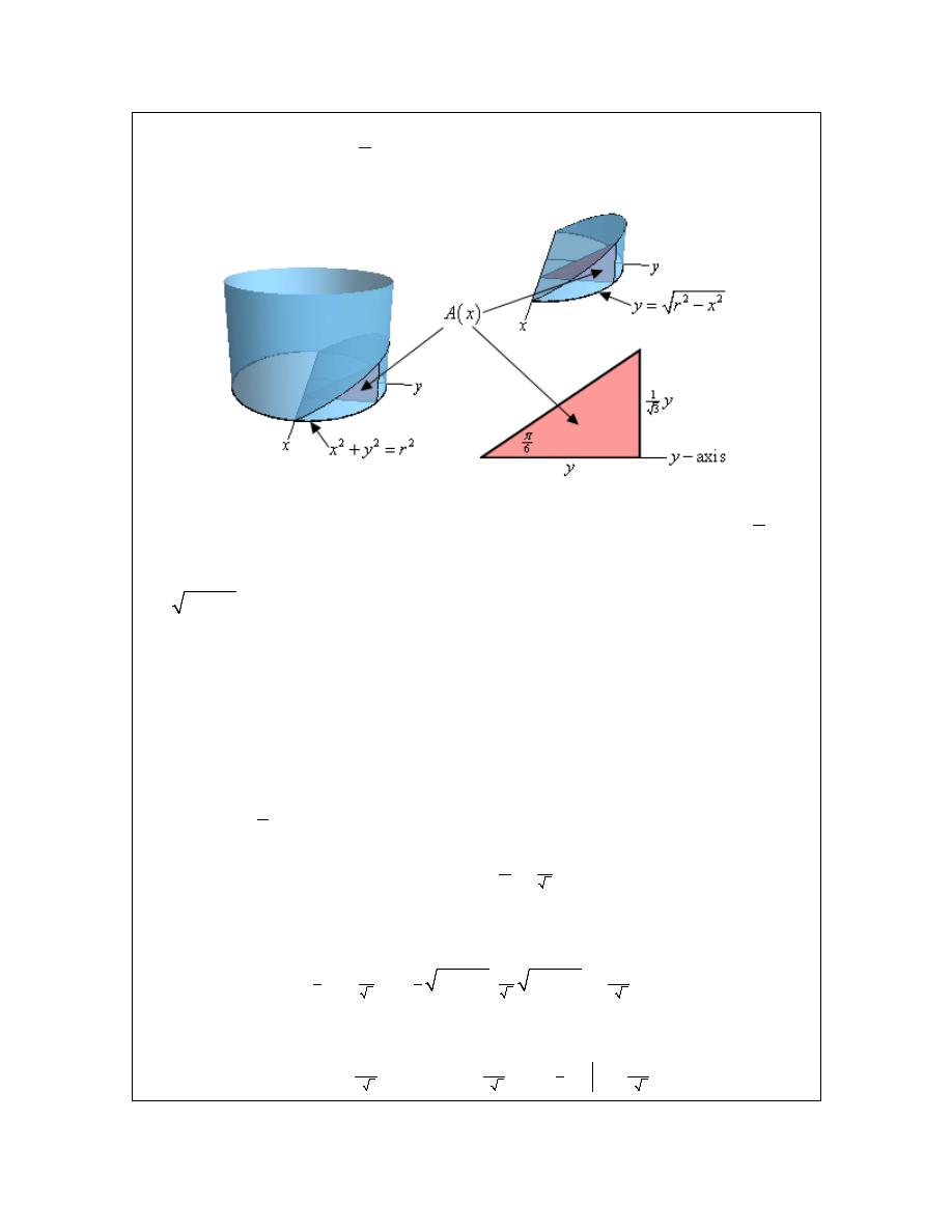
Example 4
Find the volume of a wedge cut out of a cylinder of radius r if the angle between the
top and bottom of the wedge is
6
π
.
Solution
We should really start off with a sketch of just what we’re looking for here.
On the left we see how the wedge is being cut out of the cylinder. The base of the cylinder is the
circle give by
2
2
2
x
y
r
+
=
and the angle between this circle and the top of the wedge is
6
π
. The
sketch in the upper right position is the actual wedge itself. Given the orientation of the axes here
we get the portion of the circle with positive y and so we can write the equation of the circle as
2
2
y
r
x
=
−
since we only need the positive y values. Note as well that this is the reason for
the way we oriented the axes here. We get positive y’s and we can write the equation of the circle
as a function only of x’s.
Now, as we can see in the two sketches of the wedge the cross-sectional area will be a right
triangle and the area will be a function of x as we move from the back of the cylinder, at
x
r
= −
,
to the front of the cylinder, at
x
r
=
.
The right angle of the triangle will be on the circle itself while the point on the x-axis will have an
interior angle of
6
π
. The base of the triangle will have a length of y and using a little right
triangle trig we see that the height of the rectangle is,
( )
1
6
3
height
tan
y
y
π
=
=
So, we now know the base and height of our triangle, in terms of y, and we have an equation for y
in terms of x and so we can see that the area of the triangle, i.e. the cross-sectional area is,
( ) ( )
( )
(
)
(
)
2
2
2
2
2
2
1
1
1
1
1
2
2
3
3
2 3
A x
y
y
r
x
r
x
r
x
=
=
−
−
=
−
The limits on x are
r
x
r
− ≤ ≤
and so the volume is then,
(
)
(
)
3
2
2
2
2
3
1
1
1
3
2 3
2 3
3 3
r
r
r
r
r
V
r
x
dx
r x
x
−
−
=
−
=
−
=
∫
© 2007 Paul Dawkins
41
http://tutorial.math.lamar.edu/terms.aspx
Calculus I
The next example is very similar to the previous one except it can be a little difficult to visualize
the solid itself.
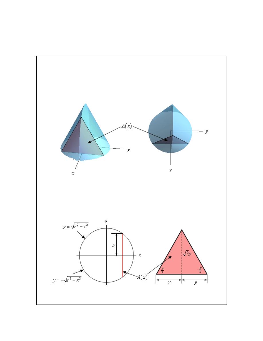
Example 5
Find the volume of the solid whose base is a disk of radius r and whose cross-
sections are equilateral triangles.
Solution
Let’s start off with a couple of sketches of this solid. The sketch on the left is from the “front” of
the solid and the sketch on the right is more from the top of the solid.
The base of this solid is the disk of radius r and we move from the back of the disk at
x
r
= −
to
the front of the disk at
x
r
=
we form equilateral triangles to form the solid. A sample equilateral
triangle, which is also the cross-sectional area, is shown above to hopefully make it a little clearer
how the solid is formed.
Now, let’s get a formula for the cross-sectional area. Let’s start with the two sketches below.
In the left hand sketch we are looking at the solid from directly above and notice that we
“reoriented” the sketch a little to put the x and y-axis in the “normal” orientation. The solid
© 2007 Paul Dawkins
42
http://tutorial.math.lamar.edu/terms.aspx
Calculus I
vertical line in this sketch is the cross-sectional area. From this we can see that the cross-section
occurs at a given x and the top half will have a length of y where the value of y will be the y-
coordinate of the point on the circle and so is,
2
2
y
r
x
=
−
Also, because the cross-section is an equilateral triangle that is centered on the x-axis the bottom
half will also have a length of y. Thus the base of the cross-section must have a length of 2y.
The sketch to the right is of one of the cross-sections. As noted above the base of the triangle has
a length of 2y. Also note that because it is an equilateral triangle the angles are all
3
π
. If we
divide the cross-section in two (as shown with the dashed line) we now have two right triangles
and using right triangle trig we can see that the length of the dashed line is,
( )
3
dashed line
tan
3
y
y
π
=
=
Therefore the height of the cross-section is
3 y
. Because the cross-section is a triangle we
know that that it’s area must then be,
( ) ( )
( )
(
)(
)
(
)
2
2
2
2
2
2
1
1
2
2
2
3
2
3
3
A x
y
y
r
x
r
x
r
x
=
=
−
−
=
−
Note that we used the cross-sectional area in terms of x because each of the cross-sections is
perpendicular to the x-axis and this pretty much forces us to integrate with respect to x.
The volume of the solid is then,
( )
(
)
(
)
2
2
2
3
3
1
4
3
3
3
3
r
r
r
r
V x
r
x
dx
r x
x
r
−
−
=
−
=
−
=
∫
The final example we’re going to work here is a little tricky both in seeing how to set it up and in
doing the integral.
© 2007 Paul Dawkins
43
http://tutorial.math.lamar.edu/terms.aspx
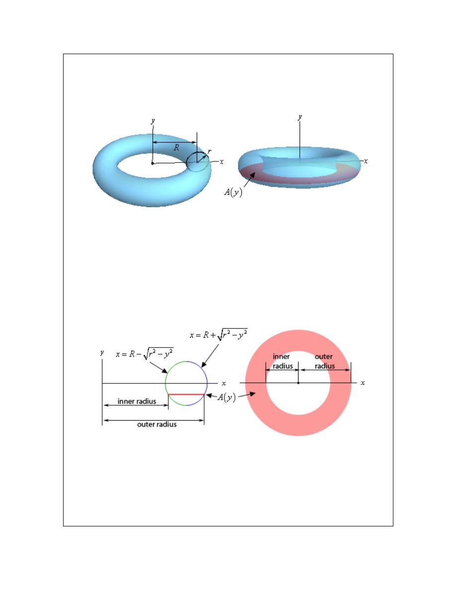
Calculus I
Example 6
Find the volume of a torus with radii r and R.
Solution
First, just what is a torus? A torus is a donut shaped solid that is generated by rotating the circle
of radius r and centered at (R, 0) about the y-axis. This is shown in the sketch to the left below.
One of the trickiest parts of this problem is seeing what the cross-sectional area needs to be.
There is an obvious one. Most people would probably think of using the circle of radius r that
we’re rotating about the y-axis as the cross-section. It is definitely one of the more obvious
choices, however setting up an integral using this is not so easy.
So, what we’ll do is use a cross-section as shown in the sketch to the right above. If we cut the
torus perpendicular to the y-axis we’ll get a cross-section of a ring and finding the area of that
shouldn’t be too bad. To do that let’s take a look at the two sketches below.
The sketch to the left is a sketch of the full cross-section. The sketch to the right is more
important however. This is a sketch of the circle that we are rotating about the y-axis. Included
is a line representing where the cross-sectional area would be in the torus.
Notice that the inner radius will always be the left portion of the circle and the outer radius will
always be the right portion of the circle. Now, we know that the equation of this is,
(
)
2
2
2
x
R
y
r
−
+
=
© 2007 Paul Dawkins
44
http://tutorial.math.lamar.edu/terms.aspx
Calculus I
and so if we solve for x we can get the equations for the left and right sides as shown above in the
sketch. This however means that we also now have equations for the inner and outer radii.
2
2
2
2
inner radius :
outer radius :
x
R
r
y
x
R
r
y
= −
−
= +
−
The cross-sectional area is then,
( )
(
)
(
)
(
) (
)
(
)
2
2
2
2
2
2
2
2
2
2
2
2
2
2
2
2
2
2
2
2
outer radius
inner radius
2
2
4
A y
R
r
y
R
r
y
R
R r
y
r
y
R
R r
y
r
y
R r
y
π
π
π
π
π
=
−
=
+
−
−
−
−
=
+
−
+ −
−
−
−
+ −
=
−
Next, the lowest cross-section will occur at
y
r
= −
and the highest cross-section will occur at
y
r
=
and so the limits for the integral will be
r
y
r
− ≤ ≤
.
The integral giving the volume is then,
2
2
2
2
2
2
0
0
4
2
4
8
r
r
r
r
V
R r
y dy
R r
y dy
R
r
y dy
π
π
π
−
=
−
=
−
=
−
∫
∫
∫
Note that we used the fact that because the integrand is an even function and we’re integrating
over
[
]
,
r r
−
we could change the lower limit to zero and double the value of the integral. We
saw this fact back in the
Substitution Rule for Definite Integrals
section.
We’ve now reached the second really tricky part of this example. With the knowledge that we’ve
currently got at this point this integral is not possible to do. It requires something called a
trig
substitution
and that is a topic for Calculus II. Luckily enough for us, and this is the tricky part,
in this case we can actually determine what the integral’s value is using what we know about
integrals.
Just for a second let’s think about a different problem. Let’s suppose we wanted to use an
integral to determine the area under the portion of the circle of radius r and centered at the origin
that is in the first quadrant. There are a couple of ways to do this, but to match what we’re doing
here let’s do the following.
We know that the equation of the circle is
2
2
2
x
y
r
+
=
and if we solve for x the equation of the
circle in the first (and fourth for that matter) quadrant is,
2
2
x
r
y
=
−
If we want an integral for the area in the first quadrant we can think of this area as the region
© 2007 Paul Dawkins
45
http://tutorial.math.lamar.edu/terms.aspx
Calculus I
between the curve
2
2
x
r
y
=
−
and the y-axis for
0
y
r
≤ ≤
and this is,
2
2
0
r
A
r
y dy
=
−
∫
In other words, this integral represents one quarter of the area of a circle of radius r and from
basic geometric formulas we now know that this integral must have the value,
2
2
2
1
4
0
r
A
r
y dy
r
π
=
−
=
∫
So, putting all this together the volume of the torus is then,
(
)
2
2
2
2
2
1
4
0
8
8
2
r
V
R
r
y dy
R
r
R
r
π
π
π
π
=
−
=
=
∫
© 2007 Paul Dawkins
46
http://tutorial.math.lamar.edu/terms.aspx
Calculus I
Work
This is the final application of integral that we’ll be looking at in this course. In this section we
will be looking at the amount of work that is done by a force in moving an object.
In a first course in Physics you typically look at the work that a constant force, F, does when
moving an object over a distance of d. In these cases the work is,
W
Fd
=
However, most forces are not constant and will depend upon where exactly the force is acting.
So, let’s suppose that the force at any x is given by F(x). Then the work done by the force in
moving an object from
x
a
=
to
x
b
=
is given by,
( )
b
a
W
F x dx
=
∫
To see a justification of this formula see the
Proof of Various Integral Properties
section of the
Extras chapter.
Notice that if the force is constant we get the correct formula for a constant force.
(
)
b
a
b
a
W
F dx
Fx
F b a
=
=
=
−
∫
where b-a is simply the distance moved, or d.
So, let’s take a look at a couple of examples of non-constant forces.
Example 1
A spring has a natural length of 20 cm. A 40 N force is required to stretch (and hold
the spring) to a length of 30 cm. How much work is done in stretching the spring from 35 cm to
38 cm?
Solution
This example will require Hooke’s Law to determine the force. Hooke’s Law tells us that the
force required to stretch a spring a distance of x meters from its natural length is,
( )
F x
k x
=
where
0
k
>
is called the spring constant.
The first thing that we need to do is determine the spring constant for this spring. We can do that
using the initial information. A force of 40 N is required to stretch the spring 30cm-20cm = 10cm
= 0.10m from its natural length. Using Hooke’s Law we have,
40
0.10
400
k
k
=
⇒
=
So, according to Hooke’s Law the force required to hold this spring x meters from its natural
© 2007 Paul Dawkins
47
http://tutorial.math.lamar.edu/terms.aspx
Calculus I
length is,
( )
400
F x
x
=
We want to know the work required to stretch the spring from 35cm to 38cm. First we need to
convert these into distances from the natural length in meters. Doing that gives us x’s of 0.15m
and 0.18m.
The work is then,
0.18
0.15
0.18
2
0.15
400
200
1.98 J
W
x dx
x
=
=
=
∫
Example 2
We have a cable that weighs 2 lbs/ft attached to a bucket filled with coal that weighs
800 lbs. The bucket is initially at the bottom of a 500 ft mine shaft. Answer each of the
following about this.
(a) Determine the amount of work required to lift the bucket to the midpoint of
the shaft.
(b) Determine the amount of work required to lift the bucket from the midpoint
of the shaft to the top of the shaft.
(c) Determine the amount of work required to lift the bucket all the way up the
shaft.
Solution
Before answering either part we first need to determine the force. In this case the force will be
the weight of the bucket and cable at any point in the shaft.
To determine a formula for this we will first need to set a convention for x. For this problem we
will set x to be the amount of cable that has been pulled up. So at the bottom of the shaft
0
x
=
,
at the midpoint of the shaft
250
x
=
and at the top of the shaft
500
x
=
. Also at any point in the
shaft there is
500
x
−
feet of cable still in the shaft.
The force then for any x is then nothing more than the weight of the cable and bucket at that
point. This is,
( )
(
)
weight of cable
weight of bucket/coal
2 500
800
1800 2
F x
x
x
=
+
=
− +
=
−
We can now answer the questions.
(a) In this case we want to know the work required to move the cable and bucket/coal from
0
x
=
to
250
x
=
. The work required is,
© 2007 Paul Dawkins
48
http://tutorial.math.lamar.edu/terms.aspx
Calculus I
( )
(
)
250
0
250
0
250
2
0
1800 2
1800
387500 ft-lb
W
F x dx
x dx
x
x
=
=
−
=
−
=
∫
∫
(b) In this case we want to move the cable and bucket/coal from
250
x
=
to
500
x
=
. The work
required is,
( )
(
)
500
250
500
250
500
2
250
1800 2
1800
262500 ft-lb
W
F x dx
x dx
x
x
=
=
−
=
−
=
∫
∫
(c) In this case the work is,
( )
(
)
500
0
500
0
500
2
0
1800 2
1800
650000 ft-lb
W
F x dx
x dx
x
x
=
=
−
=
−
=
∫
∫
Note that we could have instead just added the results from the first two parts and we would have
gotten the same answer to the third part.
Example 3
A 20 ft cable weighs 80 lbs and hangs from the ceiling of a building without
touching the floor. Determine the work that must be done to lift the bottom end of the chain all
the way up until it touches the ceiling.
Solution
First we need to determine the weight per foot of the cable. This is easy enough to get,
80 lbs
4 lb/ft
20 ft
=
Next, let x be the distance from the ceiling to any point on the cable. Using this convention we
can see that the portion of the cable in the range
10
20
x
< ≤
will actually be lifted. The portion
of the cable in the range
0
10
x
≤ ≤
will not be lifted at all since once the bottom of the cable has
been lifted up to the ceiling the cable will be doubled up and each portion will have a length of 10
ft. So, the upper 10 foot portion of the cable will never be lifted while the lower 10 ft portion will
be lifted.
© 2007 Paul Dawkins
49
http://tutorial.math.lamar.edu/terms.aspx

Calculus I
Now, the very bottom of the cable,
20
x
=
, will be lifted 10 feet to get to the midpoint and then a
further 10 feet to get to the ceiling. A point 2 feet from the bottom of the cable,
18
x
=
will lift 8
feet to get to the midpoint and then a further 8 feet until it reaches its final position (if it is 2 feet
from the bottom then its final position will be 2 feet from the ceiling). Continuing on in this
fashion we can see that for any point on the lower half of the cable, i.e.
10
20
x
≤ ≤
it will be
lifted a total of
(
)
2
10
x
−
.
As with the previous example the force required to lift any point of the cable in this range is
simply the distance that point will be lifted times the weight/foot of the cable. So, the force is
then,
( ) (
)(
)
(
)( )
(
)
distance lifted
weight per foot of cable
2
10 4
8
10
F x
x
x
=
=
−
=
−
The work required is now,
(
)
(
)
20
10
20
2
10
8
10
4
80
400 ft-lb
W
x
dx
x
x
=
−
=
−
=
∫
Provided we can find the force,
( )
F x
, for a given problem then using the above method for
determining the work is (generally) pretty simple. However, there are some problems where this
approach won’t easily work. Let’s take a look at one of those kinds of problems.
Example 4
A tank in the shape of an inverted cone has a height of 15 meters and a base radius
of 4 meters and is filled with water to a depth of 12 meters. Determine the amount of work
needed to pump all of the water to the top of the tank. Assume that the density of the water is
1000 kg/m
3
.
Solution
Okay, in this case we cannot just determine a force function,
( )
F x
that will work for us. So, we
are going to need to approach this from a different standpoint.
Let’s first set
0
x
=
to be the lower end of the tank/cone and
15
x
=
to be the top of the
tank/cone. With this definition of our x’s we can now see that the water in the tank will
correspond to the interval
[
]
0,12
.
So, let’s start off by dividing
[
]
0,12
into n subintervals each of width
x
∆
and let’s also let
*
i
x
be
© 2007 Paul Dawkins
50
http://tutorial.math.lamar.edu/terms.aspx
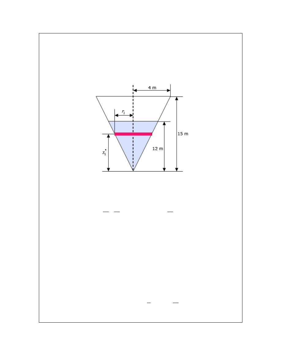
Calculus I
any point from the i
th
subinterval where
1, 2,
i
n
=
. Now, for each subinterval we will
approximate the water in the tank corresponding to that interval as a cylinder of radius
i
r
and
height
x
∆
.
Here is a quick sketch of the tank. Note that the sketch really isn’t to scale and we are looking at
the tank from directly in front so we can see all the various quantities that we need to work with.
The red strip in the sketch represents the “cylinder” of water in the i
th
subinterval. A quick
application of similar triangles will allow us to relate
i
r
to
*
i
x
(which we’ll need in a bit) as
follows.
*
*
4
4
15
15
i
i
i
i
r
r
x
x
=
⇒
=
Okay, the mass,
i
m
, of the volume of water,
i
V
, for the i
th
subinterval is simply,
density
i
i
m
V
=
×
We know the density of the water (it was given in the problem statement) and because we are
approximating the water in the i
th
subinterval as a cylinder we can easily approximate the volume,
(
) (
)
2
radius
height
i
V
π
≈
, and hence the mass of the water in the i
th
subinterval.
The mass for the i
th
subinterval is approximately,
(
)
( )
( )
2
2
2
*
*
640
4
15
9
1000
1000
i
i
i
i
m
r
x
x
x
x
x
π
π
π
≈
∆ =
∆ =
∆
To raise this volume of water we need to overcome the force of gravity that is acting on the
© 2007 Paul Dawkins
51
http://tutorial.math.lamar.edu/terms.aspx
Calculus I
volume and that is,
i
F
m g
=
, where
2
9.8
m
s
g
=
is the gravitational acceleration. The force to
raise the volume of water in the i
th
subinterval is then approximately,
( )
( )
2
*
640
9
9.8
i
i
i
F
m g
x
x
π
=
≈
∆
Next, in order to reach to the top of the tank the water in the i
th
subinterval will need to travel
approximately
*
15
i
x
−
to reach the top of the tank. Because the volume of the water in the i
th
subinterval is constant the force needed to raise the water through any distance is also a constant
force.
Therefore the work to move the volume of water in the i
th
subinterval to the top of the tank, i.e.
raise it a distance of
*
15
i
x
−
, is then approximately,
(
)
( )
( ) (
)
2
*
*
*
640
9
15
9.8
15
i
i
i
i
i
W
F
x
x
x
x
π
≈
−
=
−
∆
The total amount of work required to raise all the water to the top of the tank is then
approximately the sum of each of the
i
W
for
1, 2,
i
n
=
. Or,
( )
( ) (
)
2
*
*
640
9
1
9.8
15
n
i
i
i
W
x
x
x
π
=
≈
−
∆
∑
To get the actual amount of work we simply need to take
n
→ ∞
. I.e. compute the following
limit,
( )
( ) (
)
2
*
*
640
9
1
lim
9.8
15
n
i
i
n
i
W
x
x
x
π
→∞
=
=
−
∆
∑
This limit of a summation should look somewhat familiar to you. It’s probably been some time,
but recalling the
definition of the definite integral
we can see that this is nothing more than the
following definite integral,
( )
(
)
( )
( )
(
)
12
12
2
2
3
640
640
9
9
0
0
12
3
4
640
1
9
4
0
9.8
15
9.8
15
9.8
5
7, 566, 362.543 J
W
x
x dx
x
x dx
x
x
π
π
π
=
−
=
−
=
−
=
∫
∫
As we’ve seen in the previous example we sometimes need to compute “incremental” work and
then use that to determine the actual integral we need to compute. This idea does arise on
occasion and we shouldn’t forget it!
© 2007 Paul Dawkins
52
http://tutorial.math.lamar.edu/terms.aspx

Calculus I
© 2007 Paul Dawkins
53
http://tutorial.math.lamar.edu/terms.aspx

Calculus I
© 2007 Paul Dawkins
54
http://tutorial.math.lamar.edu/terms.aspx