
CALCULUS II
Integration Techniques
Paul Dawkins

Calculus II
Table of Contents
Preface ............................................................................................................................................ ii
Integration Techniques ................................................................................................................. 0
Introduction ................................................................................................................................................ 0
Integration by Parts .................................................................................................................................... 2
Integrals Involving Trig Functions ............................................................................................................12
Trig Substitutions ......................................................................................................................................22
Partial Fractions ........................................................................................................................................33
Integrals Involving Roots ..........................................................................................................................41
Integrals Involving Quadratics ..................................................................................................................43
Integration Strategy ...................................................................................................................................51
Improper Integrals .....................................................................................................................................58
Comparison Test for Improper Integrals ...................................................................................................65
Approximating Definite Integrals .............................................................................................................72
© 2007 Paul Dawkins
i
http://tutorial.math.lamar.edu/terms.aspx

Calculus II
Preface
Here are my online notes for my Calculus II course that I teach here at Lamar University.
Despite the fact that these are my “class notes”, they should be accessible to anyone wanting to
learn Calculus II or needing a refresher in some of the topics from the class.
These notes do assume that the reader has a good working knowledge of Calculus I topics
including limits, derivatives and basic integration and integration by substitution.
Calculus II tends to be a very difficult course for many students. There are many reasons for this.
The first reason is that this course does require that you have a very good working knowledge of
Calculus I. The Calculus I portion of many of the problems tends to be skipped and left to the
student to verify or fill in the details. If you don’t have good Calculus I skills, and you are
constantly getting stuck on the Calculus I portion of the problem, you will find this course very
difficult to complete.
The second, and probably larger, reason many students have difficulty with Calculus II is that you
will be asked to truly think in this class. That is not meant to insult anyone; it is simply an
acknowledgment that you can’t just memorize a bunch of formulas and expect to pass the course
as you can do in many math classes. There are formulas in this class that you will need to know,
but they tend to be fairly general. You will need to understand them, how they work, and more
importantly whether they can be used or not. As an example, the first topic we will look at is
Integration by Parts. The integration by parts formula is very easy to remember. However, just
because you’ve got it memorized doesn’t mean that you can use it. You’ll need to be able to look
at an integral and realize that integration by parts can be used (which isn’t always obvious) and
then decide which portions of the integral correspond to the parts in the formula (again, not
always obvious).
Finally, many of the problems in this course will have multiple solution techniques and so you’ll
need to be able to identify all the possible techniques and then decide which will be the easiest
technique to use.
So, with all that out of the way let me also get a couple of warnings out of the way to my students
who may be here to get a copy of what happened on a day that you missed.
1. Because I wanted to make this a fairly complete set of notes for anyone wanting to learn
calculus I have included some material that I do not usually have time to cover in class
and because this changes from semester to semester it is not noted here. You will need to
find one of your fellow class mates to see if there is something in these notes that wasn’t
covered in class.
2. In general I try to work problems in class that are different from my notes. However,
with Calculus II many of the problems are difficult to make up on the spur of the moment
and so in this class my class work will follow these notes fairly close as far as worked
problems go. With that being said I will, on occasion, work problems off the top of my
head when I can to provide more examples than just those in my notes. Also, I often
© 2007 Paul Dawkins
ii
http://tutorial.math.lamar.edu/terms.aspx

Calculus II
don’t have time in class to work all of the problems in the notes and so you will find that
some sections contain problems that weren’t worked in class due to time restrictions.
3. Sometimes questions in class will lead down paths that are not covered here. I try to
anticipate as many of the questions as possible in writing these up, but the reality is that I
can’t anticipate all the questions. Sometimes a very good question gets asked in class
that leads to insights that I’ve not included here. You should always talk to someone who
was in class on the day you missed and compare these notes to their notes and see what
the differences are.
4. This is somewhat related to the previous three items, but is important enough to merit its
own item. THESE NOTES ARE NOT A SUBSTITUTE FOR ATTENDING CLASS!!
Using these notes as a substitute for class is liable to get you in trouble. As already noted
not everything in these notes is covered in class and often material or insights not in these
notes is covered in class.
© 2007 Paul Dawkins
iii
http://tutorial.math.lamar.edu/terms.aspx

Calculus II
Integration Techniques
Introduction
In this chapter we are going to be looking at various integration techniques. There are a fair
number of them and some will be easier than others. The point of the chapter is to teach you
these new techniques and so this chapter assumes that you’ve got a fairly good working
knowledge of basic integration as well as substitutions with integrals. In fact, most integrals
involving “simple” substitutions will not have any of the substitution work shown. It is going to
be assumed that you can verify the substitution portion of the integration yourself.
Also, most of the integrals done in this chapter will be indefinite integrals. It is also assumed that
once you can do the indefinite integrals you can also do the definite integrals and so to conserve
space we concentrate mostly on indefinite integrals. There is one exception to this and that is the
Trig Substitution section and in this case there are some subtleties involved with definite integrals
that we’re going to have to watch out for. Outside of that however, most sections will have at
most one definite integral example and some sections will not have any definite integral
examples.
Here is a list of topics that are covered in this chapter.
– Of all the integration techniques covered in this chapter this is probably
the one that students are most likely to run into down the road in other classes.
Integrals Involving Trig Functions
– In this section we look at integrating certain products and
quotients of trig functions.
– Here we will look using substitutions involving trig functions and how they
can be used to simplify certain integrals.
– We will use partial fractions to allow us to do integrals involving some
rational functions.
– We will take a look at a substitution that can, on occasion, be used
with integrals involving roots.
Integrals Involving Quadratics
– In this section we are going to look at some integrals that
involve quadratics.
– We give a general set of guidelines for determining how to evaluate an
integral.
– We will look at integrals with infinite intervals of integration and integrals
with discontinuous integrands in this section.
© 2007 Paul Dawkins
0
http://tutorial.math.lamar.edu/terms.aspx

Calculus II
Comparison Test for Improper Integrals
– Here we will use the Comparison Test to determine
if improper integrals converge or diverge.
Approximating Definite Integrals
– There are many ways to approximate the value of a definite
integral. We will look at three of them in this section.
© 2007 Paul Dawkins
1
http://tutorial.math.lamar.edu/terms.aspx

Calculus II
Integration by Parts
Let’s start off with this section with a couple of integrals that we should already be able to do to
get us started. First let’s take a look at the following.
x
x
dx
c
=
+
∫
e
e
So, that was simple enough. Now, let’s take a look at,
2
x
x
dx
∫
e
To do this integral we’ll use the following substitution.
2
1
2
2
u
x
du
x dx
x dx
du
=
=
⇒
=
2
2
1
1
1
2
2
2
u
u
x
x
x
dx
du
c
c
=
=
+ =
+
∫
∫
e
e
e
e
Again, simple enough to do provided you remember how to do
. By the way make
sure that you can do these kinds of substitutions quickly and easily. From this point on we are
going to be doing these kinds of substitutions in our head. If you have to stop and write these out
with every problem you will find that it will take you significantly longer to do these problems.
Now, let’s look at the integral that we really want to do.
6 x
x
dx
∫
e
If we just had an x by itself or
6 x
e
by itself we could do the integral easily enough. But, we don’t
have them by themselves, they are instead multiplied together.
There is no substitution that we can use on this integral that will allow us to do the integral. So,
at this point we don’t have the knowledge to do this integral.
To do this integral we will need to use integration by parts so let’s derive the integration by parts
formula. We’ll start with the product rule.
( )
f g
f g
f g
′
′
′
=
+
Now, integrate both sides of this.
( )
f g dx
f g
f g dx
′
′
′
=
+
∫
∫
The left side is easy enough to integrate and we’ll split up the right side of the integral.
fg
f g dx
f g dx
′
′
=
+
∫
∫
Note that technically we should have had a constant of integration show up on the left side after
doing the integration. We can drop it at this point since other constants of integration will be
showing up down the road and they would just end up absorbing this one.
Finally, rewrite the formula as follows and we arrive at the integration by parts formula.
© 2007 Paul Dawkins
2
http://tutorial.math.lamar.edu/terms.aspx

Calculus II
f g dx
fg
f g dx
′
′
=
−
∫
∫
This is not the easiest formula to use however. So, let’s do a couple of substitutions.
( )
( )
( )
( )
u
f x
v
g x
du
f
x dx
dv
g x dx
=
=
′
′
=
=
Both of these are just the standard Calc I substitutions that hopefully you are used to by now.
Don’t get excited by the fact that we are using two substitutions here. They will work the same
way.
Using these substitutions gives us the formula that most people think of as the integration by parts
formula.
u dv
uv
v du
=
−
∫
∫
To use this formula we will need to identify u and dv, compute du and v and then use the formula.
Note as well that computing v is very easy. All we need to do is integrate dv.
v
dv
=
∫
So, let’s take a look at the integral above that we mentioned we wanted to do.
Example 1
Evaluate the following integral.
6 x
x
dx
∫
e
Solution
So, on some level, the problem here is the x that is in front of the exponential. If that wasn’t there
we could do the integral. Notice as well that in doing integration by parts anything that we
choose for u will be differentiated. So, it seems that choosing
u
x
=
will be a good choice since
upon differentiating the x will drop out.
Now that we’ve chosen u we know that dv will be everything else that remains. So, here are the
choices for u and dv as well as du and v.
6
6
6
1
6
x
x
x
u
x
dv
dx
du
dx
v
dx
=
=
=
=
=
∫
e
e
e
The integral is then,
6
6
6
6
6
1
6
6
1
6
36
x
x
x
x
x
x
x
dx
dx
x
c
=
−
=
−
+
⌠
⌡
∫
e
e
e
e
e
Once we have done the last integral in the problem we will add in the constant of integration to
get our final answer.
© 2007 Paul Dawkins
3
http://tutorial.math.lamar.edu/terms.aspx

Calculus II
Next, let’s take a look at integration by parts for definite integrals. The integration by parts
formula for definite integrals is,
Integration by Parts, Definite Integrals
b
b
b
a
a
a
u dv
uv
v du
=
−
∫
∫
Note that the
b
a
uv
in the first term is just the standard integral evaluation notation that you should
be familiar with at this point. All we do is evaluate the term, uv in this case, at b then subtract off
the evaluation of the term at a.
At some level we don’t really need a formula here because we know that when doing definite
integrals all we need to do is do the indefinite integral and then do the evaluation.
Let’s take a quick look at a definite integral using integration by parts.
Example 2
Evaluate the following integral.
2
6
1
x
x
dx
−
∫
e
Solution
This is the same integral that we looked at in the first example so we’ll use the same u and dv to
get,
2
2
2
6
6
6
1
1
1
2
2
6
6
1
1
12
6
1
6
6
1
6
36
11
7
36
36
x
x
x
x
x
x
x
dx
dx
x
−
−
−
−
−
−
=
−
=
−
=
+
∫
∫
e
e
e
e
e
e
e
Since we need to be able to do the indefinite integral in order to do the definite integral and doing
the definite integral amounts to nothing more than evaluating the indefinite integral at a couple of
points we will concentrate on doing indefinite integrals in the rest of this section. In fact,
throughout most of this chapter this will be the case. We will be doing far more indefinite
integrals than definite integrals.
Let’s take a look at some more examples.
Example 3
Evaluate the following integral.
(
)
3
5 cos
4
t
t
dt
+
⌠
⌡
Solution
There are two ways to proceed with this example. For many, the first thing that they try is
multiplying the cosine through the parenthesis, splitting up the integral and then doing integration
by parts on the first integral.
While that is a perfectly acceptable way of doing the problem it’s more work than we really need
© 2007 Paul Dawkins
4
http://tutorial.math.lamar.edu/terms.aspx

Calculus II
to do. Instead of splitting the integral up let’s instead use the following choices for u and dv.
3
5
cos
4
3
4 sin
4
t
u
t
dv
dt
t
du
dt
v
= +
=
=
=
The integral is then,
(
)
(
)
(
)
3
5 cos
4 3
5 sin
12 sin
4
4
4
4 3
5 sin
48 cos
4
4
t
t
t
t
dt
t
dt
t
t
t
c
+
=
+
−
=
+
+
+
⌠
⌠
⌡
⌡
Notice that we pulled any constants out of the integral when we used the integration by parts
formula. We will usually do this in order to simplify the integral a little.
Example 4
Evaluate the following integral.
(
)
2
sin 10
w
w dw
∫
Solution
For this example we’ll use the following choices for u and dv.
(
)
(
)
2
sin 10
1
2
cos 10
10
u
w
dv
w dw
du
w dw
v
w
=
=
=
= −
The integral is then,
(
)
(
)
(
)
2
2
1
sin 10
cos 10
cos 10
10
5
w
w
w dw
w
w
w dw
= −
+
∫
∫
In this example, unlike the previous examples, the new integral will also require integration by
parts. For this second integral we will use the following choices.
(
)
(
)
cos 10
1
sin 10
10
u
w
dv
w dw
du
dw
v
w
=
=
=
=
So, the integral becomes,
(
)
(
)
(
)
(
)
(
)
(
)
(
)
(
)
(
)
(
)
2
2
2
2
1
1
sin 10
cos 10
sin 10
sin 10
10
5 10
10
1
1
cos 10
sin 10
cos 10
10
5 10
100
1
cos 10
sin 10
cos 10
10
50
500
w
w
w
w dw
w
w
w dw
w
w
w
w
w
c
w
w
w
w
w
c
= −
+
−
= −
+
+
+
= −
+
+
+
∫
∫
Be careful with the coefficient on the integral for the second application of integration by parts.
Since the integral is multiplied by
1
5
we need to make sure that the results of actually doing the
integral are also multiplied by
1
5
. Forgetting to do this is one of the more common mistakes with
integration by parts problems.
© 2007 Paul Dawkins
5
http://tutorial.math.lamar.edu/terms.aspx

Calculus II
As this last example has shown us, we will sometimes need more than one application of
integration by parts to completely evaluate an integral. This is something that will happen so
don’t get excited about it when it does.
In this next example we need to acknowledge an important point about integration techniques.
Some integrals can be done in using several different techniques. That is the case with the
integral in the next example.
Example 5
Evaluate the following integral
1
x x
dx
+
∫
(a) Using Integration by Parts.
(b) Using a standard Calculus I substitution.
Solution
(a) Evaluate using Integration by Parts.
First notice that there are no trig functions or exponentials in this integral. While a good many
integration by parts integrals will involve trig functions and/or exponentials not all of them will
so don’t get too locked into the idea of expecting them to show up.
In this case we’ll use the following choices for u and dv.
(
)
3
2
1
2
1
3
u
x
dv
x
dx
du
dx
v
x
=
=
+
=
=
+
The integral is then,
(
)
(
)
(
)
(
)
3
3
2
2
3
5
2
2
2
2
1
1
1
3
3
2
4
1
1
3
15
x x
dx
x x
x
dx
x x
x
c
+
=
+
−
+
=
+
−
+
+
∫
∫
(b) Evaluate Using a standard Calculus I substitution.
Now let’s do the integral with a substitution. We can use the following substitution.
1
1
u
x
x
u
du
dx
= +
= −
=
Notice that we’ll actually use the substitution twice, once for the quantity under the square root
and once for the x in front of the square root. The integral is then,
(
)
(
)
(
)
3
1
2
2
5
3
2
2
5
3
2
2
1
1
2
2
5
3
2
2
1
1
5
3
x x
dx
u
u du
u
u du
u
u
c
x
x
c
+
=
−
=
−
=
−
+
=
+
−
+
+
∫
∫
∫
© 2007 Paul Dawkins
6
http://tutorial.math.lamar.edu/terms.aspx

Calculus II
So, we used two different integration techniques in this example and we got two different
answers. The obvious question then should be : Did we do something wrong?
Actually, we didn’t do anything wrong. We need to
remember
the following fact from Calculus
I.
( )
( )
( )
( )
If then
f
x
g x
f x
g x
c
′
′
=
=
+
In other words, if two functions have the same derivative then they will differ by no more than a
constant. So, how does this apply to the above problem? First define the following,
( )
( )
1
f
x
g x
x x
′
′
=
=
+
Then we can compute
( )
f x
and
( )
g x
by integrating as follows,
( )
( )
( )
( )
f x
f
x dx
g x
g x dx
′
′
=
=
∫
∫
We’ll use integration by parts for the first integral and the substitution for the second integral.
Then according to the fact
( )
f x
and
( )
g x
should differ by no more than a constant. Let’s
verify this and see if this is the case. We can verify that they differ by no more than a constant if
we take a look at the difference of the two and do a little algebraic manipulation and
simplification.
(
)
(
)
(
)
(
)
(
)
(
)
(
)
(
) ( )
3
5
5
3
2
2
2
2
3
2
3
2
2
4
2
2
1
1
1
1
3
15
5
3
2
4
2
2
1
1
1
3
15
5
3
1
0
0
x x
x
x
x
x
x
x
x
x
+
−
+
−
+
−
+
=
+
−
+ −
+ +
=
+
=
So, in this case it turns out the two functions are exactly the same function since the difference is
zero. Note that this won’t always happen. Sometimes the difference will yield a nonzero
constant. For an example of this check out the
notes.
So just what have we learned? First, there will, on occasion, be more than one method for
evaluating an integral. Secondly, we saw that different methods will often lead to different
answers. Last, even though the answers are different it can be shown, sometimes with a lot of
work, that they differ by no more than a constant.
When we are faced with an integral the first thing that we’ll need to decide is if there is more than
one way to do the integral. If there is more than one way we’ll then need to determine which
method we should use. The general rule of thumb that I use in my classes is that you should use
the method that you find easiest. This may not be the method that others find easiest, but that
doesn’t make it the wrong method.
© 2007 Paul Dawkins
7
http://tutorial.math.lamar.edu/terms.aspx

Calculus II
One of the more common mistakes with integration by parts is for people to get too locked into
perceived patterns. For instance, all of the previous examples used the basic pattern of taking u to
be the polynomial that sat in front of another function and then letting dv be the other function.
This will not always happen so we need to be careful and not get locked into any patterns that we
think we see.
Let’s take a look at some integrals that don’t fit into the above pattern.
Example 6
Evaluate the following integral.
ln x dx
∫
Solution
So, unlike any of the other integral we’ve done to this point there is only a single function in the
integral and no polynomial sitting in front of the logarithm.
The first choice of many people here is to try and fit this into the pattern from above and make the
following choices for u and dv.
1
ln
u
dv
x dx
=
=
This leads to a real problem however since that means v must be,
ln
v
x dx
=
∫
In other words, we would need to know the answer ahead of time in order to actually do the
problem. So, this choice simply won’t work. Also notice that with this choice we’d get that
0
du
=
which also causes problems and is another reason why this choice will not work.
Therefore, if the logarithm doesn’t belong in the dv it must belong instead in the u. So, let’s use
the following choices instead
ln
1
u
x
dv
dx
du
dx
v
x
x
=
=
=
=
The integral is then,
1
ln
ln
ln
ln
x dx
x
x
x dx
x
x
x
dx
x
x
x c
=
−
=
−
=
− +
⌠
⌡
∫
∫
Example 7
Evaluate the following integral.
5
3
1
x
x
dx
+
∫
Solution
So, if we again try to use the pattern from the first few examples for this integral our choices for u
and dv would probably be the following.
5
3
1
u
x
dv
x
dx
=
=
+
However, as with the previous example this won’t work since we can’t easily compute v.
3
1
v
x
dx
=
+
∫
© 2007 Paul Dawkins
8
http://tutorial.math.lamar.edu/terms.aspx

Calculus II
This is not an easy integral to do. However, notice that if we had an x
2
in the integral along with
the root we could very easily do the integral with a substitution. Also notice that we do have a lot
of x’s floating around in the original integral. So instead of putting all the x’s (outside of the root)
in the u let’s split them up as follows.
(
)
3
2
3
3
2
3
2
1
2
3
1
9
u
x
dv
x
x
dx
du
x dx
v
x
=
=
+
=
=
+
We can now easily compute v and after using integration by parts we get,
(
)
(
)
(
)
(
)
3
3
5
3
3
3
2
3
2
2
3
5
3
3
3
2
2
2
2
1
1
1
9
3
2
4
1
1
9
45
x
x
dx
x
x
x
x
dx
x
x
x
c
+
=
+
−
+
=
+
−
+
+
⌠
⌡
∫
So, in the previous two examples we saw cases that didn’t quite fit into any perceived pattern that
we might have gotten from the first couple of examples. This is always something that we need
to be on the lookout for with integration by parts.
Let’s take a look at another example that also illustrates another integration technique that
sometimes arises out of integration by parts problems.
Example 8
Evaluate the following integral.
cos d
θ
θ θ
∫
e
Solution
Okay, to this point we’ve always picked u in such a way that upon differentiating it would make
that portion go away or at the very least put it the integral into a form that would make it easier to
deal with. In this case no matter which part we make u it will never go away in the differentiation
process.
It doesn’t much matter which we choose to be u so we’ll choose in the following way. Note
however that we could choose the other way as well and we’ll get the same result in the end.
cos
sin
u
dv
d
du
d
v
θ
θ
θ
θ
θ θ
=
=
= −
=
e
e
The integral is then,
cos
cos
sin
d
d
θ
θ
θ
θ θ
θ
θ θ
=
+
∫
∫
e
e
e
So, it looks like we’ll do integration by parts again. Here are our choices this time.
sin
cos
u
dv
d
du
d
v
θ
θ
θ
θ
θ θ
=
=
=
=
e
e
The integral is now,
cos
cos
sin
cos
d
d
θ
θ
θ
θ
θ θ
θ
θ
θ θ
=
+
−
∫
∫
e
e
e
e
© 2007 Paul Dawkins
9
http://tutorial.math.lamar.edu/terms.aspx
Calculus II
Now, at this point it looks like we’re just running in circles. However, notice that we now have
the same integral on both sides and on the right side it’s got a minus sign in front of it. This
means that we can add the integral to both sides to get,
2
cos
cos
sin
d
θ
θ
θ
θ θ
θ
θ
=
+
∫
e
e
e
All we need to do now is divide by 2 and we’re done. The integral is,
(
)
1
cos
cos
sin
2
d
c
θ
θ
θ
θ θ
θ
θ
=
+
+
∫
e
e
e
Notice that after dividing by the two we add in the constant of integration at that point.
This idea of integrating until you get the same integral on both sides of the equal sign and then
simply solving for the integral is kind of nice to remember. It doesn’t show up all that often, but
when it does it may be the only way to actually do the integral.
We’ve got one more example to do. As we will see some problems could require us to do
integration by parts numerous times and there is a short hand method that will allow us to do
multiple applications of integration by parts quickly and easily.
Example 9
Evaluate the following integral.
4
2
x
x
dx
∫
e
Solution
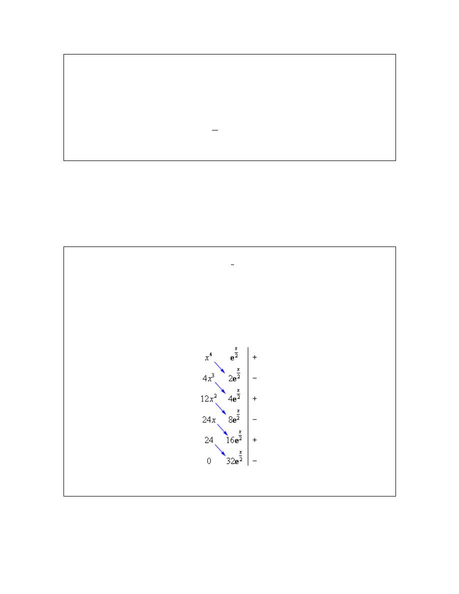
We start off by choosing u and dv as we always would. However, instead of computing du and v
we put these into the following table. We then differentiate down the column corresponding to u
until we hit zero. In the column corresponding to dv we integrate once for each entry in the first
column. There is also a third column which we will explain in a bit and it always starts with a
“+” and then alternates signs as shown.
Now, multiply along the diagonals shown in the table. In front of each product put the sign in the
third column that corresponds to the “u” term for that product. In this case this would give,
© 2007 Paul Dawkins
10
http://tutorial.math.lamar.edu/terms.aspx

Calculus II
( )
( )
(
)
(
)
( )
4
4
3
2
2
2
2
2
2
2
4
3
2
2
2
2
2
2
2
4
4
12
8
24
16
24
32
2
16
96
384
768
x
x
x
x
x
x
x
x
x
x
x
x
dx
x
x
x
x
x
x
x
x
c
=
−
+
−
+
=
−
+
−
+
+
∫
e
e
e
e
e
e
e
e
e
e
e
We’ve got the integral. This is much easier than writing down all the various u’s and dv’s that
we’d have to do otherwise.
So, in this section we’ve seen how to do integration by parts. In your later math classes this is
liable to be one of the more frequent integration techniques that you’ll encounter.
It is important to not get too locked into patterns that you may think you’ve seen. In most cases
any pattern that you think you’ve seen can (and will be) violated at some point in time. Be
careful!
Also, don’t forget the shorthand method for multiple applications of integration by parts
problems. It can save you a fair amount of work on occasion.
© 2007 Paul Dawkins
11
http://tutorial.math.lamar.edu/terms.aspx

Calculus II
Integrals Involving Trig Functions
In this section we are going to look at quite a few integrals involving trig functions and some of
the techniques we can use to help us evaluate them. Let’s start off with an integral that we should
already be able to do.
5
5
6
cos sin
using the substitution
sin
1
sin
6
x
x dx
u du
u
x
x c
=
=
=
+
∫
∫
This integral is easy to do with a substitution because the presence of the cosine, however, what
about the following integral.
Example 1
Evaluate the following integral.
5
sin x dx
∫
Solution
This integral no longer has the cosine in it that would allow us to use the substitution that we used
above. Therefore, that substitution won’t work and we are going to have to find another way of
doing this integral.
Let’s first notice that we could write the integral as follows,
(
)
2
5
4
2
sin
sin
sin
sin
sin
x dx
x
x dx
x
x dx
=
=
∫
∫
∫
Now recall the trig identity,
2
2
2
2
cos
sin
1
sin
1 cos
x
x
x
x
+
=
⇒
= −
With this identity the integral can be written as,
(
)
2
5
2
sin
1 cos
sin
x dx
x
x dx
=
−
∫
∫
and we can now use the substitution
cos
u
x
=
. Doing this gives us,
(
)
2
5
2
2
4
3
5
3
5
sin
1
1 2
2
1
3
5
2
1
cos
cos
cos
3
5
x dx
u
du
u
u du
u
u
u
c
x
x
x c
= −
−
= − −
+
= −
−
+
+
= −
+
−
+
∫
∫
∫
So, with a little rewriting on the integrand we were able to reduce this to a fairly simple
substitution.
Notice that we were able to do the rewrite that we did in the previous example because the
exponent on the sine was odd. In these cases all that we need to do is strip out one of the sines.
© 2007 Paul Dawkins
12
http://tutorial.math.lamar.edu/terms.aspx

Calculus II
The exponent on the remaining sines will then be even and we can easily convert the remaining
sines to cosines using the identity,
2
2
cos
sin
1
x
x
+
=
(1)
If the exponent on the sines had been even this would have been difficult to do. We could strip
out a sine, but the remaining sines would then have an odd exponent and while we could convert
them to cosines the resulting integral would often be even more difficult than the original integral
in most cases.
Let’s take a look at another example.
Example 2 Evaluate the following integral.
6
3
sin
cos
x
x dx
∫
Solution
So, in this case we’ve got both sines and cosines in the problem and in this case the exponent on
the sine is even while the exponent on the cosine is odd. So, we can use a similar technique in
this integral. This time we’ll strip out a cosine and convert the rest to sines.
(
)
(
)
6
3
6
2
6
2
6
2
6
8
7
9
sin
cos
sin
cos
cos
sin
1 sin
cos
sin
1
1
1
sin
sin
7
9
x
x dx
x
x
x dx
x
x
x dx
u
x
u
u
du
u
u du
x
x
c
=
=
−
=
=
−
=
−
=
−
+
∫
∫
∫
∫
∫
At this point let’s pause for a second to summarize what we’ve learned so far about integrating
powers of sine and cosine.
sin
cos
n
m
x
x dx
∫
(2)
In this integral if the exponent on the sines (n) is odd we can strip out one sine, convert the rest to
cosines using (1) and then use the substitution
cos
u
x
=
. Likewise, if the exponent on the
cosines (m) is odd we can strip out one cosine and convert the rest to sines and the use the
substitution
sin
u
x
=
.
Of course, if both exponents are odd then we can use either method. However, in these cases it’s
usually easier to convert the term with the smaller exponent.
The one case we haven’t looked at is what happens if both of the exponents are even? In this case
the technique we used in the first couple of examples simply won’t work and in fact there really
isn’t any one set method for doing these integrals. Each integral is different and in some cases
there will be more than one way to do the integral.
With that being said most, if not all, of integrals involving products of sines and cosines in which
both exponents are even can be done using one or more of the following formulas to rewrite the
integrand.
© 2007 Paul Dawkins
13
http://tutorial.math.lamar.edu/terms.aspx

Calculus II
( )
(
)
( )
(
)
( )
2
2
1
cos
1 cos 2
2
1
sin
1 cos 2
2
1
sin cos
sin 2
2
x
x
x
x
x
x
x
=
+
=
−
=
The first two formulas are the standard half angle formula from a trig class written in a form that
will be more convenient for us to use. The last is the standard double angle formula for sine,
again with a small rewrite.
Let’s take a look at an example.
Example 3
Evaluate the following integral.
2
2
sin
cos
x
x dx
∫
Solution
As noted above there are often more than one way to do integrals in which both of the exponents
are even. This integral is an example of that. There are at least two solution techniques for this
problem. We will do both solutions starting with what is probably the harder of the two, but it’s
also the one that many people see first.
Solution 1
In this solution we will use the two half angle formulas above and just substitute them into the
integral.
( )
(
)
( )
(
)
( )
2
2
2
1
1
sin
cos
1 cos 2
1 cos 2
2
2
1
1 cos
2
4
x
x dx
x
x
dx
x dx
=
−
+
=
−
⌠
⌡
∫
∫
So, we still have an integral that can’t be completely done, however notice that we have managed
to reduce the integral down to just one term causing problems (a cosine with an even power)
rather than two terms causing problems.
In fact to eliminate the remaining problem term all that we need to do is reuse the first half angle
formula given above.
( )
(
)
( )
( )
( )
2
2
1
1
sin
cos
1
1 cos 4
4
2
1
1
1
cos 4
4
2
2
1 1
1
sin 4
4 2
8
1
1
sin 4
8
32
x
x dx
x
dx
x dx
x
x
c
x
x
c
=
−
+
=
−
=
−
+
=
−
+
⌠
⌡
⌠
⌡
∫
So, this solution required a total of three trig identities to complete.
© 2007 Paul Dawkins
14
http://tutorial.math.lamar.edu/terms.aspx

Calculus II
Solution 2
In this solution we will use the half angle formula to help simplify the integral as follows.
(
)
( )
( )
2
2
2
2
2
sin
cos
sin cos
1
sin 2
2
1
sin
2
4
x
x dx
x
x
dx
x
dx
x dx
=
=
=
⌠
⌡
∫
∫
∫
Now, we use the double angle formula for sine to reduce to an integral that we can do.
( )
( )
2
2
1
sin
cos
1 cos 4
8
1
1
sin 4
8
32
x
x dx
x dx
x
x
c
=
−
=
−
+
∫
∫
This method required only two trig identities to complete.
Notice that the difference between these two methods is more one of “messiness”. The second
method is not appreciably easier (other than needing one less trig identity) it is just not as messy
and that will often translate into an “easier” process.
In the previous example we saw two different solution methods that gave the same answer. Note
that this will not always happen. In fact, more often than not we will get different answers.
However, as we discussed in the
Integration by Parts
section, the two answers will differ by no
more than a constant.
In general when we have products of sines and cosines in which both exponents are even we will
need to use a series of half angle and/or double angle formulas to reduce the integral into a form
that we can integrate. Also, the larger the exponents the more we’ll need to use these formulas
and hence the messier the problem.
Sometimes in the process of reducing integrals in which both exponents are even we will run
across products of sine and cosine in which the arguments are different. These will require one of
the following formulas to reduce the products to integrals that we can do.
(
)
(
)
(
)
(
)
(
)
(
)
1
sin
cos
sin
sin
2
1
sin
sin
cos
cos
2
1
cos
cos
cos
cos
2
α
β
α β
α β
α
β
α β
α β
α
β
α β
α β
=
−
+
+
=
−
−
+
=
−
+
+
Let’s take a look at an example of one of these kinds of integrals.
© 2007 Paul Dawkins
15
http://tutorial.math.lamar.edu/terms.aspx

Calculus II
Example 4
Evaluate the following integral.
( ) ( )
cos 15
cos 4
x
x dx
∫
Solution
This integral requires the last formula listed above.
( ) ( )
( )
( )
( )
( )
1
cos 15
cos 4
cos 11
cos 19
2
1
1
1
sin 11
sin 19
2 11
19
x
x dx
x
x dx
x
x
c
=
+
=
+
+
∫
∫
Okay, at this point we’ve covered pretty much all the possible cases involving products of sines
and cosines. It’s now time to look at integrals that involve products of secants and tangents.
This time, let’s do a little analysis of the possibilities before we just jump into examples. The
general integral will be,
sec
tan
n
m
x
x dx
∫
(3)
The first thing to notice is that we can easily convert even powers of secants to tangents and even
powers of tangents to secants by using a formula similar to (1). In fact, the formula can be
derived from (1) so let’s do that.
2
2
2
2
2
2
2
sin
cos
1
sin
cos
1
cos
cos
cos
x
x
x
x
x
x
x
+
=
+
=
2
2
tan
1 sec
x
x
+ =
(4)
Now, we’re going to want to deal with (3) similarly to how we dealt with (2). We’ll want to
eventually use one of the following substitutions.
2
tan
sec
sec
sec tan
u
x
du
x dx
u
x
du
x
x dx
=
=
=
=
So, if we use the substitution
tan
u
x
=
we will need two secants left for the substitution to work.
This means that if the exponent on the secant (n) is even we can strip two out and then convert the
remaining secants to tangents using (4).
Next, if we want to use the substitution
sec
u
x
=
we will need one secant and one tangent left
over in order to use the substitution. This means that if the exponent on the tangent (m) is odd
and we have at least one secant in the integrand we can strip out one of the tangents along with
one of the secants of course. The tangent will then have an even exponent and so we can use (4)
to convert the rest of the tangents to secants. Note that this method does require that we have at
least one secant in the integral as well. If there aren’t any secants then we’ll need to do
something different.
If the exponent on the secant is even and the exponent on the tangent is odd then we can use
either case. Again, it will be easier to convert the term with the smallest exponent.
© 2007 Paul Dawkins
16
http://tutorial.math.lamar.edu/terms.aspx

Calculus II
Let’s take a look at a couple of examples.
Example 5
Evaluate the following integral.
9
5
sec
tan
x
x dx
∫
Solution
First note that since the exponent on the secant isn’t even we can’t use the substitution
tan
u
x
=
.
However, the exponent on the tangent is odd and we’ve got a secant in the integral and so we will
be able to use the substitution
sec
u
x
=
. This means stripping out a single tangent (along with a
secant) and converting the remaining tangents to secants using (4).
Here’s the work for this integral.
(
)
(
)
9
5
8
4
2
8
2
2
8
2
12
10
8
13
11
9
sec
tan
sec
tan
tan sec
sec
sec
1 tan sec
sec
1
2
1
2
1
sec
sec
sec
13
11
9
x
x dx
x
x
x
x dx
x
x
x
x dx
u
x
u
u
du
u
u
u du
x
x
x
c
=
=
−
=
=
−
=
−
+
=
−
+
+
∫
∫
∫
∫
∫
Example 6
Evaluate the following integral.
4
6
sec
tan
x
x dx
∫
Solution
So, in this example the exponent on the tangent is even so the substitution
sec
u
x
=
won’t work.
The exponent on the secant is even and so we can use the substitution
tan
u
x
=
for this integral.
That means that we need to strip out two secants and convert the rest to tangents. Here is the
work for this integral.
(
)
(
)
4
6
2
6
2
2
6
2
2
6
8
6
9
7
sec
tan
sec
tan
sec
tan
1 tan
sec
tan
1
1
1
tan
tan
9
7
x
x dx
x
x
x dx
x
x
x dx
u
x
u
u du
u
u du
x
x
c
=
=
+
=
=
+
=
+
=
+
+
∫
∫
∫
∫
∫
Both of the previous examples fit very nicely into the patterns discussed above and so were not
all that difficult to work. However, there are a couple of exceptions to the patterns above and in
these cases there is no single method that will work for every problem. Each integral will be
different and may require different solution methods in order to evaluate the integral.
Let’s first take a look at a couple of integrals that have odd exponents on the tangents, but no
secants. In these cases we can’t use the substitution
sec
u
x
=
since it requires there to be at least
one secant in the integral.
© 2007 Paul Dawkins
17
http://tutorial.math.lamar.edu/terms.aspx

Calculus II
Example 7
Evaluate the following integral.
tan x dx
∫
Solution
To do this integral all we need to do is recall the definition of tangent in terms of sine and cosine
and then this integral is nothing more than a Calculus I substitution.
1
sin
tan
cos
cos
1
ln cos
ln
ln
ln cos
ln sec
r
x
x dx
dx
u
x
x
du
u
x
c
r
x
x
x
c
x
c
−
=
=
= −
= −
+
=
=
+
+
⌠
⌡
⌠
⌡
∫
Example 8
Evaluate the following integral.
3
tan x dx
∫
Solution
The trick to this one is do the following manipulation of the integrand.
(
)
3
2
2
2
tan
tan tan
tan
sec
1
tan sec
tan
x dx
x
x dx
x
x
dx
x
x dx
x dx
=
=
−
=
−
∫
∫
∫
∫
∫
We can now use the substitution
tan
u
x
=
on the first integral and the results from the previous
example on the second integral.
The integral is then,
3
2
1
tan
tan
ln sec
2
x dx
x
x
c
=
−
+
∫
Note that all odd powers of tangent (with the exception of the first power) can be integrated using
the same method we used in the previous example. For instance,
(
)
5
3
2
3
2
3
tan
tan
sec
1
tan
sec
tan
x dx
x
x
dx
x
x dx
x dx
=
−
=
−
∫
∫
∫
∫
So, a quick substitution (
tan
u
x
=
) will give us the first integral and the second integral will
always be the previous odd power.
Now let’s take a look at a couple of examples in which the exponent on the secant is odd and the
exponent on the tangent is even. In these cases the substitutions used above won’t work.
It should also be noted that both of the following two integrals are integrals that we’ll be seeing
on occasion in later sections of this chapter and in later chapters. Because of this it wouldn’t be a
bad idea to make a note of these results so you’ll have them ready when you need them later.
© 2007 Paul Dawkins
18
http://tutorial.math.lamar.edu/terms.aspx

Calculus II
Example 9
Evaluate the following integral.
sec x dx
∫
Solution
This one isn’t too bad once you see what you’ve got to do. By itself the integral can’t be done.
However, if we manipulate the integrand as follows we can do it.
(
)
2
sec
sec
tan
sec
sec
tan
sec
tan sec
sec
tan
x
x
x
x dx
dx
x
x
x
x
x
dx
x
x
+
=
+
+
=
+
⌠
⌡
⌠
⌡
∫
In this form we can do the integral using the substitution
sec
tan
u
x
x
=
+
. Doing this gives,
sec
ln sec
tan
x dx
x
x
c
=
+
+
∫
The idea used in the above example is a nice idea to keep in mind. Multiplying the numerator
and denominator of a term by the same term above can, on occasion, put the integral into a form
that can be integrated. Note that this method won’t always work and even when it does it won’t
always be clear what you need to multiply the numerator and denominator by. However, when it
does work and you can figure out what term you need it can greatly simplify the integral.
Here’s the next example.
Example 10
Evaluate the following integral.
3
sec x dx
∫
Solution
This one is different from any of the other integrals that we’ve done in this section. The first step
to doing this integral is to perform integration by parts using the following choices for u and dv.
2
sec
sec
sec tan
tan
u
x
dv
x dx
du
x
x dx
v
x
=
=
=
=
Note that using integration by parts on this problem is not an obvious choice, but it does work
very nicely here. After doing integration by parts we have,
3
2
sec
sec tan
sec tan
x dx
x
x
x
x dx
=
−
∫
∫
Now the new integral also has an odd exponent on the secant and an even exponent on the tangent
and so the previous examples of products of secants and tangents still won’t do us any good.
To do this integral we’ll first write the tangents in the integral in terms of secants. Again, this is
not necessarily an obvious choice but it’s what we need to do in this case.
(
)
3
2
3
sec
sec tan
sec
sec
1
sec tan
sec
sec
x dx
x
x
x
x
dx
x
x
x dx
x dx
=
−
−
=
−
+
∫
∫
∫
∫
Now, we can use the results from the previous example to do the second integral and notice that
© 2007 Paul Dawkins
19
http://tutorial.math.lamar.edu/terms.aspx

Calculus II
the first integral is exactly the integral we’re being asked to evaluate with a minus sign in front.
So, add it to both sides to get,
3
2 sec
sec tan
ln sec
tan
x dx
x
x
x
x
=
+
+
∫
Finally divide by two and we’re done.
(
)
3
1
sec
sec tan
ln sec
tan
2
x dx
x
x
x
x
c
=
+
+
+
∫
Again, note that we’ve again used the idea of integrating the right side until the original integral
shows up and then moving this to the left side and dividing by its coefficient to complete the
evaluation. We first saw this in the
Integration by Parts
section and noted at the time that this was
a nice technique to remember. Here is another example of this technique.
Now that we’ve looked at products of secants and tangents let’s also acknowledge that because
we can relate cosecants and cotangents by
2
2
1 cot
csc
x
x
+
=
all of the work that we did for products of secants and tangents will also work for products of
cosecants and cotangents. We’ll leave it to you to verify that.
There is one final topic to be discussed in this section before moving on.
To this point we’ve looked only at products of sines and cosines and products of secants and
tangents. However, the methods used to do these integrals can also be used on some quotients
involving sines and cosines and quotients involving secants and tangents (and hence quotients
involving cosecants and cotangents).
Let’s take a quick look at an example of this.
Example 11
Evaluate the following integral.
7
4
sin
cos
x
dx
x
⌠
⌡
Solution
If this were a product of sines and cosines we would know what to do. We would strip out a sine
(since the exponent on the sine is odd) and convert the rest of the sines to cosines. The same idea
will work in this case. We’ll strip out a sine from the numerator and convert the rest to cosines as
follows,
(
)
(
)
7
6
4
4
3
2
4
3
2
4
sin
sin
sin
cos
cos
sin
sin
cos
1 cos
sin
cos
x
x
dx
x dx
x
x
x
x dx
x
x
x dx
x
=
=
−
=
⌠
⌠
⌡
⌡
⌠
⌡
⌠
⌡
At this point all we need to do is use the substitution
cos
u
x
=
and we’re done.
© 2007 Paul Dawkins
20
http://tutorial.math.lamar.edu/terms.aspx

Calculus II
(
)
3
2
7
4
4
4
2
2
3
3
3
3
1
sin
cos
3
3
1 1
1
1
3
3
3
3
1
3
1
3cos
cos
3cos
cos
3
u
x
dx
du
x
u
u
u
u du
u
u
c
u
u
x
x
c
x
x
−
−
−
= −
= −
−
+ −
= − −
+
+
−
+
=
−
−
+
+
⌠
⌠
⌡
⌡
∫
So, under the right circumstances, we can use the ideas developed to help us deal with products of
trig functions to deal with quotients of trig functions. The natural question then, is just what are
the right circumstances?
First notice that if the quotient had been reversed as in this integral,
4
7
cos
sin
x
dx
x
⌠
⌡
we wouldn’t have been able to strip out a sine.
4
4
7
6
cos
cos
1
sin
sin
sin
x
x
dx
dx
x
x
x
=
⌠
⌠
⌡
⌡
In this case the “stripped out” sine remains in the denominator and it won’t do us any good for the
substitution
cos
u
x
=
since this substitution requires a sine in the numerator of the quotient.
Also note that, while we could convert the sines to cosines, the resulting integral would still be a
fairly difficult integral.
So, we can use the methods we applied to products of trig functions to quotients of trig functions
provided the term that needs parts stripped out in is the numerator of the quotient.
© 2007 Paul Dawkins
21
http://tutorial.math.lamar.edu/terms.aspx

Calculus II
Trig Substitutions
As we have done in the last couple of sections, let’s start off with a couple of integrals that we
should already be able to do with a standard substitution.
(
)
3
2
2
2
2
2
1
1
25
4
25
4
25
4
75
25
25
4
x
x
x
dx
x
c
dx
x
c
x
−
=
−
+
=
− +
−
⌠
⌡
∫
Both of these used the substitution
2
25
4
u
x
=
−
and at this point should be pretty easy for you to
do. However, let’s take a look at the following integral.
Example 1
Evaluate the following integral.
2
25
4
x
dx
x
−
⌠
⌡
Solution
In this case the substitution
2
25
4
u
x
=
−
will not work and so we’re going to have to do
something different for this integral.
It would be nice if we could get rid of the square root somehow. The following substitution will
do that for us.
2
sec
5
x
θ
=
Do not worry about where this came from at this point. As we work the problem you will see that
it works and that if we have a similar type of square root in the problem we can always use a
similar substitution.
Before we actually do the substitution however let’s verify the claim that this will allow us to get
rid of the square root.
(
)
2
2
2
2
4
25
4
25
sec
4
4 sec
1
2 sec
1
25
x
θ
θ
θ
− =
− =
− =
−
To get rid of the square root all we need to do is recall the relationship,
2
2
2
2
tan
1 sec
sec
1
tan
θ
θ
θ
θ
+ =
⇒
− =
Using this fact the square root becomes,
2
2
25
4
2 tan
2 tan
x
θ
θ
− =
=
Note the presence of the absolute value bars there. These are important. Recall that
2
x
x
=
There should always be absolute value bars at this stage. If we knew that
tan
θ
was always
positive or always negative we could eliminate the absolute value bars using,
if 0
if 0
x
x
x
x
x
≥
=
−
<
© 2007 Paul Dawkins
22
http://tutorial.math.lamar.edu/terms.aspx
Calculus II
Without limits we won’t be able to determine if
tan
θ
is positive or negative, however, we will
need to eliminate them in order to do the integral. Therefore, since we are doing an indefinite
integral we will assume that
tan
θ
will be positive and so we can drop the absolute value bars.
This gives,
2
25
4
2 tan
x
θ
− =
So, we were able to eliminate the square root using this substitution. Let’s now do the
substitution and see what we get. In doing the substitution don’t forget that we’ll also need to
substitute for the dx. This is easy enough to get from the substitution.
2
2
sec
sec tan
5
5
x
dx
d
θ
θ
θ θ
=
⇒
=
Using this substitution the integral becomes,
2
2
5
2
25
4
2 tan
2
sec tan
sec
5
2 tan
x
dx
d
x
d
θ
θ
θ θ
θ
θ θ
−
=
=
⌠
⌠
⌡
⌡
∫
With this substitution we were able to reduce the given integral to an integral involving trig
functions and we saw how to do these problems in the previous
. Let’s finish the integral.
(
)
2
2
25
4
2 sec
1
2 tan
x
dx
d
x
c
θ
θ
θ θ
−
=
−
=
−
+
⌠
⌡
∫
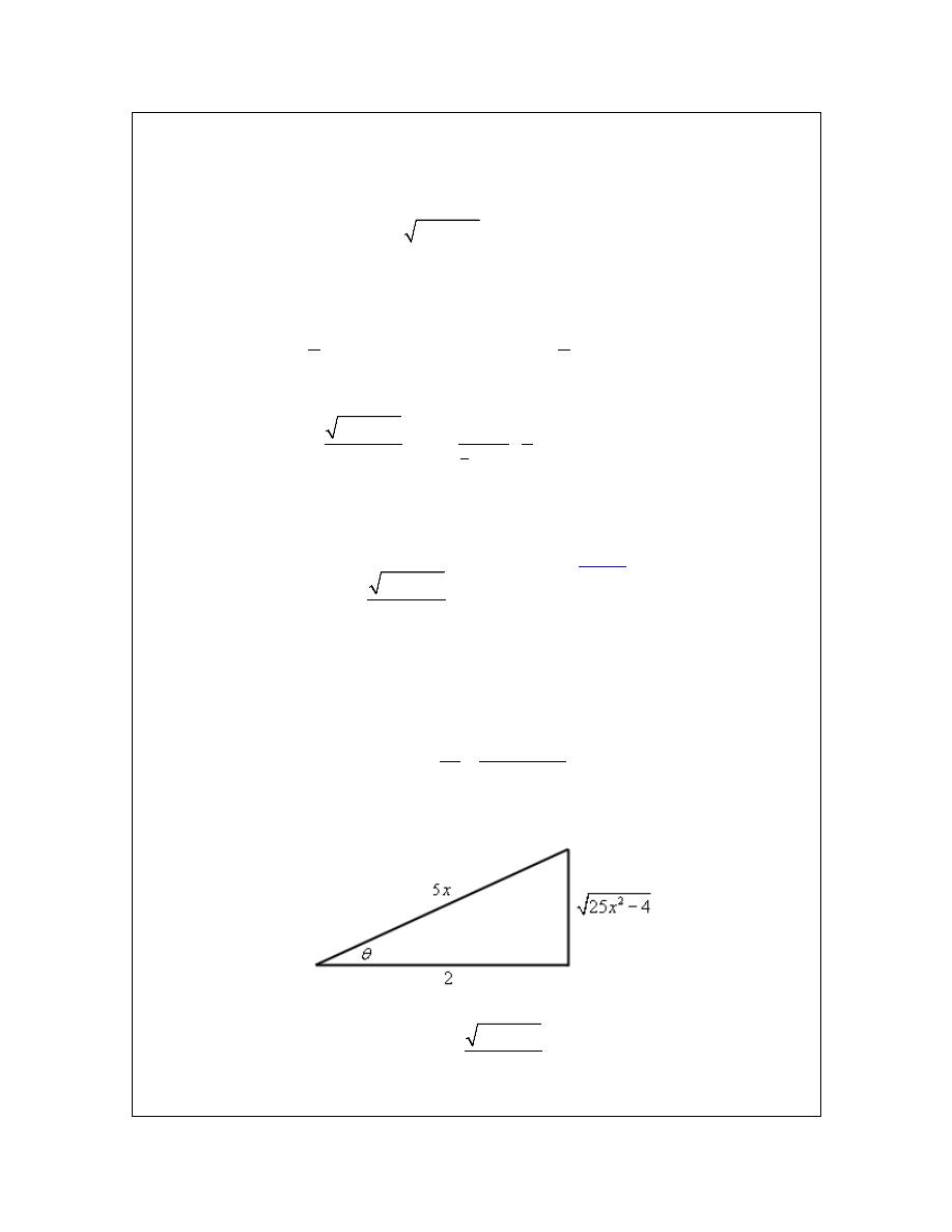
So, we’ve got an answer for the integral. Unfortunately the answer isn’t given in x’s as it should
be. So, we need to write our answer in terms of x. We can do this with some right triangle trig.
From our original substitution we have,
5
hypotenuse
sec
2
adjacent
x
θ =
=
This gives the following right triangle.
From this we can see that,
2
25
4
tan
2
x
θ
−
=
We can deal with the
θ
in one of any variety of ways. From our substitution we can see that,
© 2007 Paul Dawkins
23
http://tutorial.math.lamar.edu/terms.aspx

Calculus II
1
5
sec
2
x
θ
−
=
While this is a perfectly acceptable method of dealing with the
θ
we can use any of the possible
six inverse trig functions and since sine and cosine are the two trig functions most people are
familiar with we will usually use the inverse sine or inverse cosine. In this case we’ll use the
inverse cosine.
1
2
cos
5x
θ
−
=
So, with all of this the integral becomes,
2
2
1
2
1
25
4
25
4
2
2
cos
2
5
2
25
4
2 cos
5
x
x
dx
c
x
x
x
c
x
−
−
−
−
=
−
+
=
− −
+
⌠
⌡
We now have the answer back in terms of x.
Wow! That was a lot of work. Most of these won’t take as long to work however. This first one
needed lot’s of explanation since it was the first one. The remaining examples won’t need quite
as much explanation and so won’t take as long to work.
However, before we move onto more problems let’s first address the issue of definite integrals
and how the process differs in these cases.
Example 2
Evaluate the following integral.
4
2
5
2
5
25
4
x
dx
x
−
⌠
⌡
Solution
The limits here won’t change the substitution so that will remain the same.
2
sec
5
x
θ
=
Using this substitution the square root still reduces down to,
2
25
4
2 tan
x
θ
− =
However, unlike the previous example we can’t just drop the absolute value bars. In this case
we’ve got limits on the integral and so we can use the limits as well as the substitution to
determine the range of
θ
that we’re in. Once we’ve got that we can determine how to drop the
absolute value bars.
Here’s the limits of
θ
.
© 2007 Paul Dawkins
24
http://tutorial.math.lamar.edu/terms.aspx

Calculus II
2
2
2
sec
0
5
5
5
4
4
2
sec
5
5
5
3
x
x
θ
θ
π
θ
θ
=
⇒
=
⇒
=
=
⇒
=
⇒
=
So, if we are in the range
2
4
5
5
x
≤ ≤
then
θ
is in the range of
3
0
π
θ
≤ ≤
and in this range of
θ
’s
tangent is positive and so we can just drop the absolute value bars.
Let’s do the substitution. Note that the work is identical to the previous example and so most of it
is left out. We’ll pick up at the final integral and then do the substitution.
(
)
4
2
5
2
3
0
2
5
3
0
25
4
2
sec
1
2 tan
2
2 3
3
x
dx
d
x
π
π
θ
θ
θ θ
π
−
=
−
=
−
=
−
⌠
⌡
∫
Note that because of the limits we didn’t need to resort to a right triangle to complete the
problem.
Let’s take a look at a different set of limits for this integral.
Example 3
Evaluate the following integral.
2
2
5
4
5
25
4
x
dx
x
−
−
−
⌠
⌡
Solution
Again, the substitution and square root are the same as the first two examples.
2
2
sec
25
4
2 tan
5
x
x
θ
θ
=
− =
Let’s next see the limits
θ
for this problem.
2
2
2
sec
5
5
5
4
4
2
2
sec
5
5
5
3
x
x
θ
θ π
π
θ
θ
= −
⇒
− =
⇒
=
= −
⇒
− =
⇒
=
Note that in determining the value of
θ
we used the smallest positive value. Now for this range
of x’s we have
2
3
π
θ π
≤ ≤
and in this range of
θ
tangent is negative and so in this case we can
drop the absolute value bars, but will need to add in a minus sign upon doing so. In other words,
2
25
4
2 tan
x
θ
− = −
So, the only change this will make in the integration process is to put a minus sign in front of the
integral. The integral is then,
© 2007 Paul Dawkins
25
http://tutorial.math.lamar.edu/terms.aspx
Calculus II
(
)
2
2
5
2
2
4
3
5
2
3
25
4
2
sec
1
2 tan
2
2 3
3
x
dx
d
x
π
π
π
π
θ
θ
θ θ
π
−
−
−
= −
−
= −
−
=
−
⌠
⌡
∫
In the last two examples we saw that we have to be very careful with definite integrals. We need
to make sure that we determine the limits on
θ
and whether or not this will mean that we can
drop the absolute value bars or if we need to add in a minus sign when we drop them.
Before moving on to the next example let’s get the general form for the substitution that we used
in the previous set of examples.
2
2
2
sec
a
b x
a
x
b
θ
−
⇒
=
Let’s work a new and different type of example.
Example 4
Evaluate the following integral.
4
2
1
9
dx
x
x
−
⌠
⌡
Solution
Now, the square root in this problem looks to be (almost) the same as the previous ones so let’s
try the same type of substitution and see if it will work here as well.
3sec
x
θ
=
Using this substitution the square root becomes,
2
2
2
2
9
9 9 sec
3 1 sec
3
tan
x
θ
θ
θ
−
=
−
=
−
=
−
So using this substitution we will end up with a negative quantity (the tangent squared is always
positive of course) under the square root and this will be trouble. Using this substitution will give
complex values and we don’t want that. So, using secant for the substitution won’t work.
However, the following substitution (and differential) will work.
3sin
3cos
x
dx
d
θ
θ θ
=
=
With this substitution the square root is,
2
2
2
9
3 1 sin
3 cos
3 cos
3cos
x
θ
θ
θ
θ
−
=
−
=
=
=
We were able to drop the absolute value bars because we are doing an indefinite integral and so
we’ll assume that everything is positive.
The integral is now,
© 2007 Paul Dawkins
26
http://tutorial.math.lamar.edu/terms.aspx
Calculus II
(
)
4
4
2
4
4
1
1
3cos
81sin
3cos
9
1
1
81
sin
1
csc
81
dx
d
x
x
d
d
θ θ
θ
θ
θ
θ
θ θ
=
−
=
=
⌠
⌠
⌡
⌡
⌠
⌡
∫
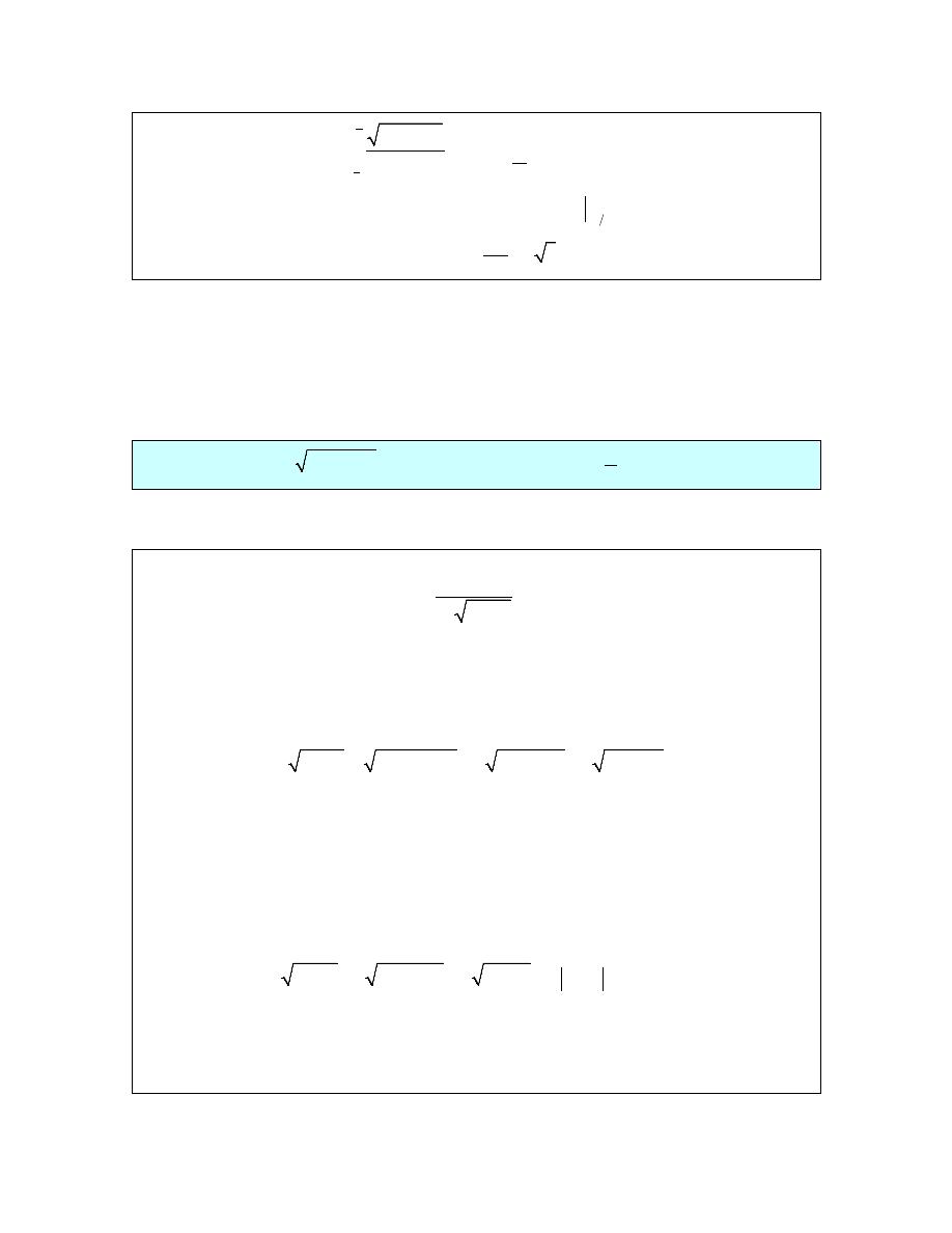
In the previous section we saw how to deal with integrals in which the exponent on the secant
was even and since cosecants behave an awful lot like secants we should be able to do something
similar with this.
Here is the integral.
(
)
2
2
4
2
2
2
2
3
1
1
csc
csc
81
9
1
cot
1 csc
cot
81
1
1
81
1
1
cot
cot
81 3
dx
d
x
x
d
u
u
du
c
θ
θ θ
θ
θ θ
θ
θ
θ
=
−
=
+
=
= −
+
= −
+
+
⌠
⌡
∫
∫
∫
Now we need to go back to x’s using a right triangle. Here is the right triangle for this problem
and trig functions for this problem.
2
9
sin
cot
3
x
x
x
θ
θ
−
=
=
The integral is then,
(
)
3
2
2
4
2
3
2
2
2
3
1
1
1
9
9
81 3
9
9
9
243
81
x
x
dx
c
x
x
x
x
x
x
c
x
x
−
−
= −
+
+
−
−
−
= −
−
+
⌠
⌡
Here’s the general form for this type of square root.
© 2007 Paul Dawkins
27
http://tutorial.math.lamar.edu/terms.aspx

Calculus II
2
2
2
sin
a
a
b x
x
b
θ
−
⇒
=
There is one final case that we need to look at. The next integral will also contain something that
we need to make sure we can deal with.
Example 5
Evaluate the following integral.
(
)
1
6
5
3
2
2
0
36
1
x
dx
x
+
⌠
⌡
Solution
First, notice that there really is a square root in this problem even though it isn’t explicitly written
out. To see the root let’s rewrite things a little.
(
)
(
)
(
)
3
3
1
3
2
2
2
2
2
36
1
36
1
36
1
x
x
x
+
=
+
=
+
This square root is not in the form we saw in the previous examples. Here we will use the
substitution for this root.
2
1
1
tan
sec
6
6
x
dx
d
θ
θ θ
=
=
With this substitution the denominator becomes,
(
) (
) (
)
3
3
3
3
2
2
2
36
1
tan
1
sec
sec
x
θ
θ
θ
+
=
+
=
=
Now, because we have limits we’ll need to convert them to
θ
so we can determine how to drop
the absolute value bars.
1
0
0
tan
0
6
1
1
1
tan
6
6
6
4
x
x
θ
θ
π
θ
θ
=
⇒
=
⇒
=
=
⇒
=
⇒
=
In this range of
θ
secant is positive and so we can drop the absolute value bars.
Here is the integral,
(
)
1
6
5
5
1
4
2
7776
3
3
2
0
2
0
5
4
0
tan
1
sec
sec
6
36
1
1
tan
46656
sec
x
dx
d
x
d
π
π
θ
θ θ
θ
θ θ
θ
=
+
=
⌠
⌠
⌡
⌡
⌠
⌡
There are several ways to proceed from this point. Normally with an odd exponent on the tangent
we would strip one of them out and convert to secants. However, that would require that we also
© 2007 Paul Dawkins
28
http://tutorial.math.lamar.edu/terms.aspx
Calculus II
have a secant in the numerator which we don’t have. Therefore, it seems like the best way to do
this one would be to convert the integrand to sines and cosines.
(
)
(
)
1
6
5
5
4
3
4
2
0
2
0
2
2
4
4
0
1
sin
46656
cos
36
1
1 cos
1
sin
46656
cos
x
dx
d
x
d
π
π
θ θ
θ
θ
θ θ
θ
=
+
−
=
⌠
⌠
⌡
⌡
⌠
⌡
We can now use the substitution
cos
u
θ
=
and we might as well convert the limits as well.
0
cos 0 1
2
cos
4
4
2
u
u
θ
π
π
θ
=
=
=
=
=
=
The integral is then,
(
)
1
6
2
5
4
2
2
3
1
2
2
0
2
2
3
1
1
2
1
46656
36
1
1
1
2
46656
3
1
11 2
17496
279936
x
dx
u
u
du
x
u
u
u
−
−
= −
−
+
+
= −
−
+ +
=
−
⌠
⌡
∫
The general form for this final type of square root is
2
2
2
tan
a
a
b x
x
b
θ
+
⇒
=
We have a couple of final examples to work in this section. Not all trig substitutions will just
jump right out at us. Sometimes we need to do a little work on the integrand first to get it into the
correct form and that is the point of the remaining examples.
Example 6
Evaluate the following integral.
2
2
4
7
x
dx
x
x
−
−
⌠
⌡
Solution
In this case the quantity under the root doesn’t obviously fit into any of the cases we looked at
above and in fact isn’t in the any of the forms we saw in the previous examples. Note however
that if we complete the square on the quadratic we can make it look somewhat like the above
integrals.
Remember that completing the square requires a coefficient of one in front of the x
2
. Once we
have that we take half the coefficient of the x, square it, and then add and subtract it to the
© 2007 Paul Dawkins
29
http://tutorial.math.lamar.edu/terms.aspx
Calculus II
quantity. Here is the completing the square for this problem.
(
)
(
)
2
2
2
2
7
7
9
2
2
2
2
1 1
2
1
2
1
9
2
2
2
x
x
x
x
x
x
−
−
=
−
+ − −
=
−
−
=
−
−
So, the root becomes,
(
)
2
2
2
4
7
2
1
9
x
x
x
−
− =
−
−
This looks like a secant substitution except we don’t just have an x that is squared. That is okay,
it will work the same way.
3
3
3
1
sec
1
sec
sec tan
2
2
2
x
x
dx
d
θ
θ
θ
θ θ
− =
= +
=
Using this substitution the root reduces to,
(
)
2
2
2
2
2
4
7
2
1
9
9 sec
9
3 tan
3 tan
3 tan
x
x
x
θ
θ
θ
θ
−
− =
−
− =
− =
=
=
Note we could drop the absolute value bars since we are doing an indefinite integral. Here is the
integral.
3
2
2
2
1
sec
3
sec tan
3 tan
2
2
4
7
1
3
sec
sec
2
2
1
3
ln sec
tan
tan
2
2
x
dx
d
x
x
d
c
θ
θ
θ θ
θ
θ
θ θ
θ
θ
θ
+
=
−
−
=
+
=
+
+
+
⌠
⌠
⌡
⌡
⌠
⌡
And here is the right triangle for this problem.
(
)
2
2
1
2
4
7
sec
tan
3
3
x
x
x
θ
θ
−
−
−
=
=
The integral is then,
(
)
2
2
2
2
1
1
2
4
7
2
4
7
ln
3
3
2
2
2
4
7
x
x
x
x
x
x
dx
c
x
x
−
−
−
−
−
=
+
+
+
−
−
⌠
⌡
© 2007 Paul Dawkins
30
http://tutorial.math.lamar.edu/terms.aspx
Calculus II
Example 7
Evaluate the following integral.
4
2
1
x
x
dx
+
∫
e
e
Solution
This doesn’t look to be anything like the other problems in this section. However it is. To see
this we first need to notice that,
( )
2
2 x
x
=
e
e
With this we can use the following substitution.
2
tan
sec
x
x
dx
d
θ
θ θ
=
=
e
e
Remember that to compute the differential all we do is differentiate both sides and then tack on
dx or
d
θ
onto the appropriate side.
With this substitution the square root becomes,
( )
2
2
2
2
1
1
1 tan
sec
sec
sec
x
x
θ
θ
θ
θ
+
=
+
=
+
=
=
=
e
e
Again, we can drop the absolute value bars because we are doing an indefinite integral. Here’s
the integral.
( )
( )
(
)
(
)
(
)
4
2
3
2
3
2
3
2
2
2
4
2
5
3
1
1
1
tan
sec
sec
sec
1 sec
sec tan
sec
1
1
sec
sec
5
3
x
x
x
x
x
x
x
x
dx
dx
dx
d
d
u
u
u du
c
θ
θ
θ θ
θ
θ
θ
θ θ
θ
θ
θ
+
=
+
=
+
=
=
−
=
=
−
=
−
+
∫
∫
∫
∫
∫
∫
e
e
e e
e
e
e
e
Here is the right triangle for this integral.
2
2
1
tan
sec
1
1
1
x
x
x
θ
θ
+
=
=
=
+
e
e
e
The integral is then,
(
)
(
)
5
3
4
2
2
2
2
2
1
1
1
1
1
5
3
x
x
x
x
dx
c
+
=
+
−
+
+
∫
e
e
e
e
© 2007 Paul Dawkins
31
http://tutorial.math.lamar.edu/terms.aspx
Calculus II
So, as we’ve seen in the final two examples in this section some integrals that look nothing like
the first few examples can in fact be turned into a trig substitution problem with a little work.
Before leaving this section let’s summarize all three cases in one place.
2
2
2
2
2
2
2
2
2
sin
sec
tan
a
a
b x
x
b
a
b x
a
x
b
a
a
b x
x
b
θ
θ
θ
−
⇒
=
−
⇒
=
+
⇒
=
© 2007 Paul Dawkins
32
http://tutorial.math.lamar.edu/terms.aspx

Calculus II
Partial Fractions
In this section we are going to take a look at integrals of rational expressions of polynomials and
once again let’s start this section out with an integral that we can already do so we can contrast it
with the integrals that we’ll be doing in this section.
(
)
2
2
2
2
1
1
using
6 and
2
1
6
ln
6
x
dx
du
u
x
x
du
x
dx
x
x
u
x
x
c
−
=
=
− −
=
−
− −
=
− − +
⌠
⌠
⌡
⌡
So, if the numerator is the derivative of the denominator (or a constant multiple of the derivative
of the denominator) doing this kind of integral is fairly simple. However, often the numerator
isn’t the derivative of the denominator (or a constant multiple). For example, consider the
following integral.
2
3
11
6
x
dx
x
x
+
− −
⌠
⌡
In this case the numerator is definitely not the derivative of the denominator nor is it a constant
multiple of the derivative of the denominator. Therefore, the simple substitution that we used
above won’t work. However, if we notice that the integrand can be broken up as follows,
2
3
11
4
1
6
3
2
x
x
x
x
x
+
=
−
− −
−
+
then the integral is actually quite simple.
2
3
11
4
1
6
3
2
4 ln
3
ln
2
x
dx
dx
x
x
x
x
x
x
c
+
=
−
− −
−
+
=
− −
+ +
⌠
⌠
⌡
⌡
This process of taking a rational expression and decomposing it into simpler rational expressions
that we can add or subtract to get the original rational expression is called partial fraction
decomposition. Many integrals involving rational expressions can be done if we first do partial
fractions on the integrand.
So, let’s do a quick review of partial fractions. We’ll start with a rational expression in the form,
( )
( )
( )
P x
f x
Q x
=
where both P(x) and Q(x) are polynomials and the degree of P(x) is smaller than the degree of
Q(x). Recall that the degree of a polynomial is the largest exponent in the polynomial. Partial
fractions can only be done if the degree of the numerator is strictly less than the degree of the
denominator. That is important to remember.
So, once we’ve determined that partial fractions can be done we factor the denominator as
completely as possible. Then for each factor in the denominator we can use the following table to
determine the term(s) we pick up in the partial fraction decomposition.
© 2007 Paul Dawkins
33
http://tutorial.math.lamar.edu/terms.aspx

Calculus II
Factor in
denominator
Term in partial
fraction decomposition
ax b
+
A
ax b
+
(
)
k
ax b
+
(
)
(
)
1
2
2
k
k
A
A
A
ax b
ax b
ax b
+
+ +
+
+
+
,
1, 2, 3,
k
=
2
ax
bx
c
+
+
2
Ax
B
ax
bx
c
+
+
+
(
)
2
k
ax
bx c
+
+
(
)
(
)
1
1
2
2
2
2
2
2
k
k
k
A x
B
A x
B
A x
B
ax
bx c
ax
bx c
ax
bx c
+
+
+
+
+ +
+
+
+
+
+
+
,
1, 2, 3,
k
=
Notice that the first and third cases are really special cases of the second and fourth cases
respectively.
There are several methods for determining the coefficients for each term and we will go over each
of those in the following examples.
Let’s start the examples by doing the integral above.
Example 1
Evaluate the following integral.
2
3
11
6
x
dx
x
x
+
− −
⌠
⌡
Solution
The first step is to factor the denominator as much as possible and get the form of the partial
fraction decomposition. Doing this gives,
(
)(
)
3
11
3
2
3
2
x
A
B
x
x
x
x
+
=
+
−
+
−
+
The next step is to actually add the right side back up.
(
)(
)
(
)
(
)
(
)(
)
2
3
3
11
3
2
3
2
A x
B x
x
x
x
x
x
+
+
−
+
=
−
+
−
+
Now, we need to choose A and B so that the numerators of these two are equal for every x. To do
this we’ll need to set the numerators equal.
(
)
(
)
3
11
2
3
x
A x
B x
+ =
+ +
−
Note that in most problems we will go straight from the general form of the decomposition to this
step and not bother with actually adding the terms back up. The only point to adding the terms is
to get the numerator and we can get that without actually writing down the results of the addition.
At this point we have one of two ways to proceed. One way will always work, but is often more
work. The other, while it won’t always work, is often quicker when it does work. In this case
both will work and so we’ll use the quicker way for this example. We’ll take a look at the other
method in a later example.
© 2007 Paul Dawkins
34
http://tutorial.math.lamar.edu/terms.aspx

Calculus II
What we’re going to do here is to notice that the numerators must be equal for any x that we
would choose to use. In particular the numerators must be equal for
2
x
= −
and
3
x
=
. So, let’s
plug these in and see what we get.
( )
( )
( )
( )
2
5
0
5
1
3
20
5
0
4
x
A
B
B
x
A
B
A
= −
=
+
−
⇒
= −
=
=
+
⇒
=
So, by carefully picking the x’s we got the unknown constants to quickly drop out. Note that
these are the values we claimed they would be above.
At this point there really isn’t a whole lot to do other than the integral.
2
3
11
4
1
6
3
2
4
1
3
2
4 ln
3
ln
2
x
dx
dx
x
x
x
x
dx
dx
x
x
x
x
c
+
=
−
− −
−
+
=
−
−
+
=
− −
+ +
⌠
⌠
⌡
⌡
⌠
⌠
⌡
⌡
Recall that to do this integral we first split it up into two integrals and then used the substitutions,
3
2
u
x
v
x
= −
= +
on the integrals to get the final answer.
Before moving onto the next example a couple of quick notes are in order here. First, many of
the integrals in partial fractions problems come down to the type of integral seen above. Make
sure that you can do those integrals.
There is also another integral that often shows up in these kinds of problems so we may as well
give the formula for it here since we are already on the subject.
1
2
2
1
1
tan
x
dx
c
x
a
a
a
−
=
+
+
⌠
⌡
It will be an example or two before we use this so don’t forget about it.
Now, let’s work some more examples.
Example 2
Evaluate the following integral.
2
3
2
4
3
4
4
x
dx
x
x
x
+
+
−
⌠
⌡
Solution
We won’t be putting as much detail into this solution as we did in the previous example. The first
thing is to factor the denominator and get the form of the partial fraction decomposition.
(
)(
)
2
4
2 3
2
2
3
2
x
A
B
C
x x
x
x
x
x
+
= +
+
+
−
+
−
The next step is to set numerators equal. If you need to actually add the right side together to get
© 2007 Paul Dawkins
35
http://tutorial.math.lamar.edu/terms.aspx

Calculus II
the numerator for that side then you should do so, however, it will definitely make the problem
quicker if you can do the addition in your head to get,
(
)(
)
(
)
(
)
2
4
2 3
2
3
2
2
x
A x
x
Bx
x
Cx x
+ =
+
− +
− +
+
As with the previous example it looks like we can just pick a few values of x and find the
constants so let’s do that.
( )( )
( )( )
0
4
2
2
1
1
2
8
2
8
2
2
40
2
8
40
5
3
9
3
3
16
2
x
A
A
x
B
B
x
C
C
=
=
−
⇒
= −
= −
=
−
−
⇒
=
=
=
⇒
=
=
Note that unlike the first example most of the coefficients here are fractions. That is not unusual
so don’t get excited about it when it happens.
Now, let’s do the integral.
2
5
1
2
2
3
2
4
1
3
4
4
2
3
2
1
5
ln
ln
2
ln 3
2
2
6
x
dx
dx
x
x
x
x
x
x
x
x
x
c
+
= − +
+
+
−
+
−
= −
+
+ +
− +
⌠
⌠
⌡
⌡
Again, as noted above, integrals that generate natural logarithms are very common in these
problems so make sure you can do them.
Example 3
Evaluate the following integral.
(
)
(
)
2
2
2
29
5
4
3
x
x
dx
x
x
−
+
−
+
⌠
⌡
Solution
This time the denominator is already factored so let’s just jump right to the partial fraction
decomposition.
(
)
(
)
(
)
2
2
2
2
2
29
5
4
3
4
3
4
x
x
A
B
Cx
D
x
x
x
x
x
−
+
+
=
+
+
−
+
−
+
−
Setting numerators gives,
(
)
(
) (
)
(
)(
)
2
2
2
2
29
5
4
3
3
4
x
x
A x
x
B x
Cx
D
x
−
+ =
−
+ +
+ +
+
−
In this case we aren’t going to be able to just pick values of x that will give us all the constants.
Therefore, we will need to work this the second (and often longer) way. The first step is to
multiply out the right side and collect all the like terms together. Doing this gives,
(
)
(
)
(
)
2
3
2
29
5
4
8
3
16
8
12
3
16
x
x
A C x
A
B
C
D x
A
C
D x
A
B
D
−
+ =
+
+ −
+ −
+
+
+
−
−
+
+
Now we need to choose A, B, C, and D so that these two are equal. In other words we will need
to set the coefficients of like powers of x equal. This will give a system of equations that can be
solved.
© 2007 Paul Dawkins
36
http://tutorial.math.lamar.edu/terms.aspx

Calculus II
3
2
1
0
:
0
:
4
8
1
1,
5,
1,
2
:
3
16
8
29
:
12
3
16
5
x
A C
x
A
B
C
D
A
B
C
D
x
A
C
D
x
A
B
D
+ =
−
+ −
+ =
⇒
=
= −
= −
=
+
−
= −
−
+
+
=
Note that we used x
0
to represent the constants. Also note that these systems can often be quite
large and have a fair amount of work involved in solving them. The best way to deal with these
is to use some form of computer aided solving techniques.
Now, let’s take a look at the integral.
(
)
(
)
(
)
(
)
2
2
2
2
2
2
2
2
2
1
29
5
1
5
2
4
3
4
3
4
1
5
2
4
3
3
4
5
1
2
ln
4
ln
3
tan
4
2
3
3
x
x
x
dx
dx
x
x
x
x
x
x
dx
x
x
x
x
x
x
x
c
x
−
−
+
− +
=
−
+
−
+
−
+
−
=
−
−
+
−
+
+
−
=
− +
−
+ +
+
−
⌠
⌠
⌡
⌡
⌠
⌡
In order to take care of the third term we needed to split it up into two separate terms. Once
we’ve done this we can do all the integrals in the problem. The first two use the substitution
4
u
x
= −
, the third uses the substitution
2
3
v
x
=
+
and the fourth term uses the formula given
above for inverse tangents.
Example 4
Evaluate the following integral.
(
)
(
)
3
2
2
2
10
3
36
1
4
x
x
x
dx
x
x
+
+
+
−
+
⌠
⌡
Solution
Let’s first get the general form of the partial fraction decomposition.
(
)
(
)
(
)
3
2
2
2
2
2
2
10
3
36
1
4
1
4
4
x
x
x
A
Bx C
Dx
E
x
x
x
x
x
+
+
+
+
+
=
+
+
−
+
−
+
+
Now, set numerators equal, expand the right side and collect like terms.
(
)
(
)(
)
(
)
(
)(
)
(
)
(
)
(
)
(
)
2
3
2
2
2
4
3
2
10
3
36
4
1
4
1
8
4
4
4
16
4
x
x
x
A x
Bx C
x
x
Dx
E
x
A
B x
C
B x
A
B C
D x
B
C
D
E x
A
C
E
+
+
+
=
+
+
+
−
+ +
+
−
=
+
+
−
+
+
− +
+
−
+
− +
+
−
−
Setting coefficient equal gives the following system.
© 2007 Paul Dawkins
37
http://tutorial.math.lamar.edu/terms.aspx

Calculus II
4
3
2
1
0
:
0
:
1
:
8
4
10
2,
2,
1,
1,
0
:
4
4
3
:
16
4
36
x
A
B
x
C
B
x
A
B C
D
A
B
C
D
E
x
B
C
D
E
x
A
C
E
+ =
− =
+
− + =
⇒
=
= −
= −
=
=
−
+
− + =
−
− =
Don’t get excited if some of the coefficients end up being zero. It happens on occasion.
Here’s the integral.
(
)
(
)
(
)
(
)
3
2
2
2
2
2
2
2
2
2
2
2
1
2
10
3
36
2
2
1
1
4
1
4
4
2
2
1
1
4
4
4
1
1
1
2 ln
1
ln
4
tan
2
2
2
4
x
x
x
x
x
dx
dx
x
x
x
x
x
x
x
dx
x
x
x
x
x
x
x
c
x
−
+
+
+
− −
=
+
+
−
+
−
+
+
=
−
−
+
−
+
+
+
=
− −
+ −
−
+
+
⌠
⌠
⌡
⌡
⌠
⌡
To this point we’ve only looked at rational expressions where the degree of the numerator was
strictly less that the degree of the denominator. Of course not all rational expressions will fit into
this form and so we need to take a look at a couple of examples where this isn’t the case.
Example 5
Evaluate the following integral.
4
3
2
3
2
5
6
18
3
x
x
x
dx
x
x
−
+
−
−
⌠
⌡
Solution
So, in this case the degree of the numerator is 4 and the degree of the denominator is 3.
Therefore, partial fractions can’t be done on this rational expression.
To fix this up we’ll need to do long division on this to get it into a form that we can deal with.
Here is the work for that.
(
)
(
)
3
2
4
3
2
4
3
3
2
3
2
2
3
5
6
18
3
2
6
18
2
6
18
x
x
x
x
x
x
x
x
x
x
x
x
−
−
−
+
−
−
−
−
+
−
− −
+
−
So, from the long division we see that,
© 2007 Paul Dawkins
38
http://tutorial.math.lamar.edu/terms.aspx

Calculus II
4
3
2
3
2
3
2
5
6
18
18
2
3
3
x
x
x
x
x
x
x
x
−
+
−
= − −
−
−
and the integral becomes,
4
3
2
3
2
3
2
3
2
5
6
18
18
2
3
3
18
2
3
x
x
x
dx
x
dx
x
x
x
x
x
dx
dx
x
x
−
+
−
=
− −
−
−
=
−
−
−
⌠
⌠
⌡
⌡
⌠
⌡
∫
The first integral we can do easily enough and the second integral is now in a form that allows us
to do partial fractions. So, let’s get the general form of the partial fractions for the second
integrand.
(
)
2
2
18
3
3
A
B
C
x
x
x
x
x
= +
+
−
−
Setting numerators equal gives us,
(
)
(
)
2
18
3
3
Ax x
B x
Cx
=
− +
− +
Now, there is a variation of the method we used in the first couple of examples that will work
here. There are a couple of values of x that will allow us to quickly get two of the three constants,
but there is no value of x that will just hand us the third.
What we’ll do in this example is pick x’s to get the two constants that we can easily get and then
we’ll just pick another value of x that will be easy to work with (i.e. it won’t give large/messy
numbers anywhere) and then we’ll use the fact that we also know the other two constants to find
the third.
( )
( )
( )
( )
0
18
3
6
3
18
9
2
1
18
2
2
2
14
2
x
B
B
x
C
C
x
A
B
C
A
A
=
=
−
⇒
= −
=
=
⇒
=
=
=
− +
− + = −
+
⇒
= −
The integral is then,
4
3
2
3
2
2
2
5
6
18
2
6
2
2
3
3
1
6
2
2 ln
2 ln
3
2
x
x
x
dx
x
dx
dx
x
x
x
x
x
x
x
x
x
c
x
−
+
−
=
−
− − −
+
−
−
=
−
+
− −
− +
⌠
⌠
⌡
⌡
∫
In the previous example there were actually two different ways of dealing with the x
2
in the
denominator. One is to treat it as a quadratic which would give the following term in the
decomposition
2
Ax
B
x
+
and the other is to treat it as a linear term in the following way,
(
)
2
2
0
x
x
=
−
which gives the following two terms in the decomposition,
© 2007 Paul Dawkins
39
http://tutorial.math.lamar.edu/terms.aspx

Calculus II
2
A
B
x
x
+
We used the second way of thinking about it in our example. Notice however that the two will
give identical partial fraction decompositions. So, why talk about this? Simple. This will work
for x
2
, but what about x
3
or x
4
? In these cases we really will need to use the second way of
thinking about these kinds of terms.
3
4
2
3
2
3
4
A
B
C
A
B
C
D
x
x
x
x
x
x
x
x
x
⇒
+
+
⇒
+
+
+
Let’s take a look at one more example.
Example 6
Evaluate the following integral.
2
2
1
x
dx
x
−
⌠
⌡
Solution
In this case the numerator and denominator have the same degree. As with the last example we’ll
need to do long division to get this into the correct form. I’ll leave the details of that to you to
check.
2
2
2
2
1
1
1
1
1
1
x
dx
dx
dx
dx
x
x
x
=
+
=
+
−
−
−
⌠
⌠
⌠
⌡
⌡
⌡
∫
So, we’ll need to partial fraction the second integral. Here’s the decomposition.
(
)(
)
1
1
1
1
1
A
B
x
x
x
x
=
+
−
+
−
+
Setting numerator equal gives,
(
)
(
)
1
1
1
A x
B x
=
+ +
−
Picking value of x gives us the following coefficients.
( )
( )
1
1
1
2
2
1
1
1
2
2
x
B
B
x
A
A
= −
=
−
⇒
= −
=
=
⇒
=
The integral is then,
2
1
1
2
2
2
1
1
1
1
1
ln
1
ln
1
2
2
x
dx
dx
dx
x
x
x
x
x
x
c
=
+
−
−
−
+
= +
− −
+ +
⌠
⌠
⌡
⌡
∫
© 2007 Paul Dawkins
40
http://tutorial.math.lamar.edu/terms.aspx
Calculus II
Integrals Involving Roots
In this section we’re going to look at an integration technique that can be useful for some
integrals with roots in them. We’ve already seen some integrals with roots in them. Some can be
done quickly with a simple Calculus I substitution and some can be done with trig substitutions.
However, not all integrals with roots will allow us to use one of these methods. Let’s look at a
couple of examples to see another technique that can be used on occasion to help with these
integrals.
Example 1
Evaluate the following integral.
3
2
3
x
dx
x
+
−
⌠
⌡
Solution
Sometimes when faced with an integral that contains a root we can use the following substitution
to simplify the integral into a form that can be easily worked with.
3
3
u
x
=
−
So, instead of letting u be the stuff under the radical as we often did in Calculus I we let u be the
whole radical. Now, there will be a little more work here since we will also need to know what x
is so we can substitute in for that in the numerator and so we can compute the differential, dx.
This is easy enough to get however. Just solve the substitution for x as follows,
3
2
3
3
x
u
dx
u du
=
+
=
Using this substitution the integral is now,
(
)
(
)
(
)
3
2
4
5
2
5
2
3
3
3
2
3
3
15
3
15
5
2
3
15
3
3
5
2
u
u du
u
u du
u
u
u
c
x
x
c
+ +
=
+
=
+
+
=
−
+
−
+
⌠
⌡
∫
So, sometimes, when an integral contains the root
( )
n
g x
the substitution,
( )
n
u
g x
=
can be used to simplify the integral into a form that we can deal with.
Let’s take a look at another example real quick.
Example 2
Evaluate the following integral.
2
3
10
dx
x
x
−
+
⌠
⌡
Solution
We’ll do the same thing we did in the previous example. Here’s the substitution and the extra
work we’ll need to do to get x in terms of u.
© 2007 Paul Dawkins
41
http://tutorial.math.lamar.edu/terms.aspx

Calculus II
2
10
10
2
u
x
x
u
dx
u du
=
+
=
−
=
With this substitution the integral is,
( )
2
2
2
2
4
2
10 3
3
10
3
10
u
dx
u du
du
u
u
u
u
x
x
=
=
− −
−
−
−
+
⌠
⌠
⌠
⌡
⌡
⌡
This integral can now be done with partial fractions.
(
)(
)
4
5
2
5
2
u
A
B
u
u
u
u
=
+
−
+
−
+
Setting numerators equal gives,
(
)
(
)
4
2
5
u
A u
B u
=
+ +
−
Picking value of u gives the coefficients.
( )
( )
8
2
8
7
7
20
5
20
7
7
u
B
B
u
A
A
= −
− =
−
=
=
=
=
The integral is then,
20
8
7
7
2
5
2
3
10
20
8
ln
5
ln
2
7
7
20
8
ln
10
5
ln
10
2
7
7
dx
du
u
u
x
x
u
u
c
x
x
c
=
+
−
+
−
+
=
− +
+ +
=
+
− +
+
+ +
⌠
⌠
⌡
⌡
So, we’ve seen a nice method to eliminate roots from the integral and put it into a form that we
can deal with. Note however, that this won’t always work and sometimes the new integral will be
just as difficult to do.
© 2007 Paul Dawkins
42
http://tutorial.math.lamar.edu/terms.aspx

Calculus II
Integrals Involving Quadratics
To this point we’ve seen quite a few integrals that involve quadratics. A couple of examples are,
2
1
2
2
2
1
1
1
ln
tan
2
x
x
dx
x
a
c
dx
x
a
x
a
a
a
−
=
± +
=
±
+
⌠
⌠
⌡
⌡
We also saw that integrals involving
2
2
2
b x
a
−
,
2
2
2
a
b x
−
and
2
2
2
a
b x
+
could be done
with a trig substitution.
Notice however that all of these integrals were missing an x term. They all consist of a quadratic
term and a constant.
Some integrals involving general quadratics are easy enough to do. For instance, the following
integral can be done with a quick substitution.
(
)
(
)
2
2
2
2
3
1
1
4
12
1
4 2
3
4
12
1
4
1
ln 4
12
1
4
x
dx
du
u
x
x
du
x
dx
x
x
u
x
x
c
+
=
=
+
−
=
+
+
−
=
+
− +
⌠
⌠
⌡
⌡
Some integrals with quadratics can be done with partial fractions. For instance,
2
10
6
4
2
2
4 ln
5
ln 3
1
3
16
5
5
3
1
3
x
dx
dx
x
x
c
x
x
x
x
−
=
−
=
+ −
+ +
+
+
+
+
⌠
⌠
⌡
⌡
Unfortunately, these methods won’t work on a lot of integrals. A simple substitution will only
work if the numerator is a constant multiple of the derivative of the denominator and partial
fractions will only work if the denominator can be factored.
This section is how to deal with integrals involving quadratics when the techniques that we’ve
looked at to this point simply won’t work.
Back in the
Trig Substitution
section we saw how to deal with square roots that had a general
quadratic in them. Let’s take a quick look at another one like that since the idea involved in
doing that kind of integral is exactly what we are going to need for the other integrals in this
section.
Example 1
Evaluate the following integral.
2
4
5
x
x
dx
+
+
∫
Solution
Recall from the Trig Substitution section that in order to do a trig substitution here we first
needed to complete the square on the quadratic. This gives,
(
)
2
2
2
4
5
4
4 4 5
2
1
x
x
x
x
x
+
+ =
+
+ − + =
+
+
After completing the square the integral becomes,
(
)
2
2
4
5
2
1
x
x
dx
x
dx
+
+
=
+
+
∫
∫
© 2007 Paul Dawkins
43
http://tutorial.math.lamar.edu/terms.aspx
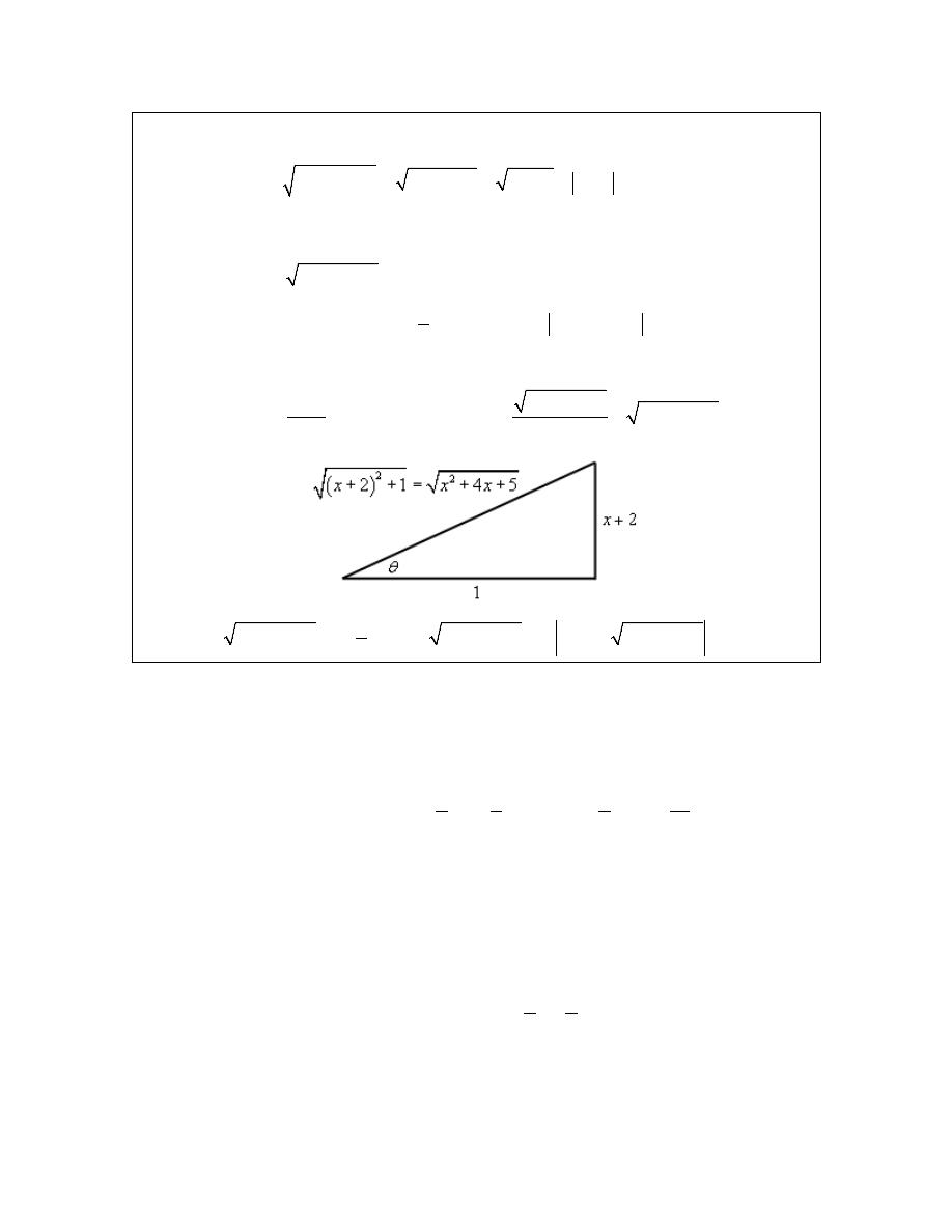
Calculus II
Upon doing this we can identify the trig substitution that we need. Here it is,
2
2
tan
tan
2
sec
x
x
dx
d
θ
θ
θ θ
+ =
=
−
=
(
)
2
2
2
2
1
tan
1
sec
sec
sec
x
θ
θ
θ
θ
+
+ =
+ =
=
=
Recall that since we are doing an indefinite integral we can drop the absolute value bars. Using
this substitution the integral becomes,
(
)
2
3
4
5
sec
1
sec tan
ln sec
tan
2
x
x
dx
d
c
θ θ
θ
θ
θ
θ
+
+
=
=
+
+
+
∫
∫
We can finish the integral out with the following right triangle.
2
2
2
4
5
tan
sec
4
5
1
1
x
x
x
x
x
θ
θ
+
+
+
=
=
=
+
+
(
)
(
)
2
2
2
1
4
5
2
4
5
ln
2
4
5
2
x
x
dx
x
x
x
x
x
x
c
+
+
=
+
+
+ +
+ +
+
+
+
∫
So, by completing the square we were able to take an integral that had a general quadratic in it
and convert it into a form that allowed us to use a known integration technique.
Let’s do a quick review of completing the square before proceeding. Here is the general
completing the square formula that we’ll use.
2
2
2
2
2
2
2
2
2
4
b
b
b
b
x
bx
c
x
bx
c
x
c
+
+ =
+
+
−
+ =
+
+ −
This will always take a general quadratic and write it in terms of a squared term and a constant
term.
Recall as well that in order to do this we must have a coefficient of one in front of the x
2
. If not
we’ll need to factor out the coefficient before completing the square. In other words,
2
2
complete the
square on this!
b
c
ax
bx c
a x
x
a
a
+
+ =
+
+
© 2007 Paul Dawkins
44
http://tutorial.math.lamar.edu/terms.aspx

Calculus II
Now, let’s see how completing the square can be used to do integrals that we aren’t able to do at
this point.
Example 2
Evaluate the following integral.
2
1
2
3
2
dx
x
x
−
+
⌠
⌡
Solution
Okay, this doesn’t factor so partial fractions just won’t work on this. Likewise, since the
numerator is just “1” we can’t use the substitution
2
2
3
8
u
x
x
=
−
+
. So, let’s see what happens
if we complete the square on the denominator.
2
2
2
2
3
2
3
2
2
1
2
3
9
9
2
1
2
16
16
3
7
2
4
16
x
x
x
x
x
x
x
−
+ =
−
+
=
−
+
−
+
−
+
With this the integral is,
(
)
2
2
3
7
4
16
1
1
1
2
3
2
2
dx
dx
x
x
x
=
−
+
−
+
⌠
⌠
⌡
⌡
Now this may not seem like all that great of a change. However, notice that we can now use the
following substitution.
3
4
u
x
du
dx
= −
=
and the integral is now,
2
2
7
16
1
1
1
2
3
2
2
dx
du
x
x
u
=
−
+
+
⌠
⌠
⌡
⌡
We can now see that this is an inverse tangent! So, using the formula from above we get,
1
2
1
1
1
4
4
tan
2
3
2
2
7
7
2
4
3
tan
7
7
u
dx
c
x
x
x
c
−
−
=
+
−
+
−
=
+
⌠
⌡
Example 3
Evaluate the following integral.
2
3
1
10
28
x
dx
x
x
−
+
+
⌠
⌡
Solution
This example is a little different from the previous one. In this case we do have an x in the
numerator however the numerator still isn’t a multiple of the derivative of the denominator and so
a simple Calculus I substitution won’t work.
© 2007 Paul Dawkins
45
http://tutorial.math.lamar.edu/terms.aspx
Calculus II
So, let’s again complete the square on the denominator and see what we get,
(
)
2
2
2
10
28
10
25 25 28
5
3
x
x
x
x
x
+
+
=
+
+
−
+
=
+
+
Upon completing the square the integral becomes,
(
)
2
2
3
1
3
1
10
28
5
3
x
x
dx
dx
x
x
x
−
−
=
+
+
+
+
⌠
⌠
⌡
⌡
At this point we can use the same type of substitution that we did in the previous example. The
only real difference is that we’ll need to make sure that we plug the substitution back into the
numerator as well.
5
5
u
x
x
u
dx
du
= +
= −
=
(
)
(
)
2
2
2
2
2
1
2
1
3
5
1
3
1
10
28
3
3
16
3
3
3
16
ln
3
tan
2
3
3
3
16
5
ln
5
3
tan
2
3
3
u
x
dx
du
x
x
u
u
du
u
u
u
u
c
x
x
c
−
−
− −
−
=
+
+
+
=
−
+
+
=
+ −
+
+
=
+
+ −
+
⌠
⌠
⌡
⌡
⌠
⌡
So, in general when dealing with an integral in the form,
2
Ax
B
dx
ax
bx
c
+
+
+
⌠
⌡
(1)
Here we are going to assume that the denominator doesn’t factor and the numerator isn’t a
constant multiple of the derivative of the denominator. In these cases we complete the square on
the denominator and then do a substitution that will yield an inverse tangent and/or a logarithm
depending on the exact form of the numerator.
Let’s now take a look at a couple of integrals that are in the same general form as (1) except the
denominator will also be raised to a power. In other words, let’s look at integrals in the form,
(
)
2
n
Ax
B
dx
ax
bx c
+
+
+
⌠
⌡
(2)
Example 4
Evaluate the following integral.
(
)
3
2
6
11
x
dx
x
x
−
+
⌠
⌡
Solution
For the most part this integral will work the same as the previous two with one exception that will
© 2007 Paul Dawkins
46
http://tutorial.math.lamar.edu/terms.aspx

Calculus II
occur down the road. So, let’s start by completing the square on the quadratic in the denominator.
(
)
2
2
2
6
11
6
9 9 11
3
2
x
x
x
x
x
−
+ =
−
+ − + =
−
+
The integral is then,
(
)
(
)
3
3
2
2
6
11
3
2
x
x
dx
dx
x
x
x
=
−
+
−
+
⌠
⌠
⌡
⌡
Now, we will use the same substitution that we’ve used to this point in the previous two
examples.
3
3
u
x
x
u
dx
du
= −
= +
=
(
)
(
)
(
)
(
)
3
3
2
2
3
3
2
2
3
6
11
2
3
2
2
x
u
dx
du
x
x
u
u
du
du
u
u
+
=
−
+
+
=
+
+
+
⌠
⌠
⌡
⌡
⌠
⌠
⌡
⌡
Now, here is where the differences start cropping up. The first integral can be done with the
substitution
2
2
v
u
=
+
and isn’t too difficult. The second integral however, can’t be done with
the substitution used on the first integral and it isn’t an inverse tangent.
It turns out that a trig substitution will work nicely on the second integral and it will be the same
as we did
we had square roots in the problem.
2
2 tan
2 sec
u
du
d
θ
θ θ
=
=
With these two substitutions the integrals become,
(
)
(
)
(
)
(
)
(
)
(
)
(
)
(
)
(
)
(
)
2
3
3
3
2
2
2
3
2
2
2
2
3
2
2
2
4
2
4
2
2
1
1
3
2 sec
2
6
11
2 tan
2
1 1
3 2 sec
4
8 tan
1
1
1
3 2
sec
4
8
2
sec
1
1
3 2
1
4
8
sec
3
2
1
1
3 2
cos
4
8
3
2
x
dx
dv
d
v
x
x
d
v
d
u
d
x
d
x
θ θ
θ
θ
θ
θ
θ
θ
θ
θ
θ
θ θ
=
+
−
+
+
= −
+
+
= −
+
+
= −
+
−
+
= −
+
−
+
⌠
⌠
⌠
⌡
⌡
⌡
⌠
⌡
⌠
⌡
⌠
⌡
∫
© 2007 Paul Dawkins
47
http://tutorial.math.lamar.edu/terms.aspx
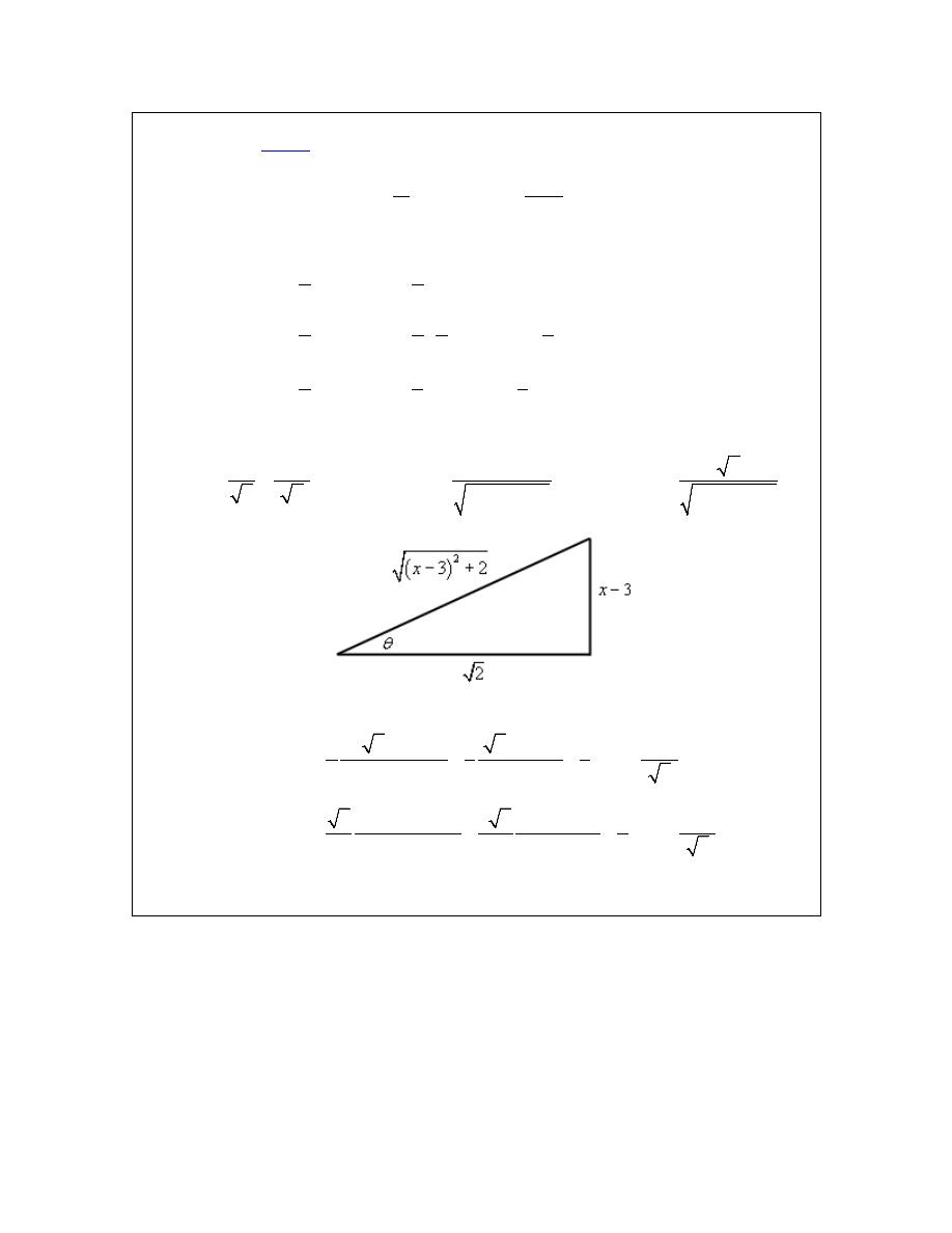
Calculus II
Okay, at this point we’ve got two options for the remaining integral. We can either use the ideas
we learned in the
about integrals involving trig integrals or we could use the following
formula.
1
2
1
1
cos
sin cos
cos
m
m
m
m
d
d
m
m
θ θ
θ
θ
θ θ
−
−
−
=
+
∫
∫
Let’s use this formula to do the integral.
4
3
2
3
0
0
3
1
3
cos
sin cos
cos
4
4
1
3 1
1
sin cos
sin cos
cos
cos
1!
4
4 2
2
1
3
3
sin cos
sin cos
4
8
8
d
d
d
θ θ
θ
θ
θ θ
θ
θ
θ
θ
θ θ
θ
θ
θ
θ
θ
θ
=
+
=
+
+
=
=
+
+
∫
∫
∫
Next, let’s use the following right triangle to get this back to x’s.
(
)
(
)
2
2
3
3
2
tan
sin
cos
2
2
3
2
3
2
u
x
x
x
x
θ
θ
θ
−
−
=
=
=
=
−
+
−
+
The cosine integral is then,
(
)
(
)
(
)
(
)
(
)
(
)
(
)
(
)
4
1
2
2
2
1
2
2
2
2 2
3
2
3
1
3
3
3
cos
tan
4
8
8
2
3
2
3
2
2
3
3 2
3
3
3
tan
2
8
8
2
3
2
3
2
x
x
x
d
x
x
x
x
x
x
x
θ θ
−
−
−
−
−
=
+
+
−
+
−
+
−
−
−
=
+
+
−
+
−
+
∫
All told then the original integral is,
© 2007 Paul Dawkins
48
http://tutorial.math.lamar.edu/terms.aspx
Calculus II
(
)
(
)
(
)
(
)
(
)
(
)
(
)
(
)
(
)
3
2
2
2
1
2
2
2
1
2
2
2
1
1
4
6
11
3
2
3 2
2
3
3 2
3
3
3
tan
8
2
8
8
2
3
2
3
2
1
3
11
9
3
9 2
3
tan
8
32
64
2
3
2
3
2
x
dx
x
x
x
x
x
x
x
x
x
x
x
c
x
x
−
−
= −
+
−
+
−
+
−
−
−
+
+
−
+
−
+
−
−
−
=
+
+
+
−
+
−
+
⌠
⌡
It’s a long and messy answer, but there it is.
Example 5
Evaluate the following integral.
(
)
2
2
3
4 2
x
dx
x
x
−
−
−
⌠
⌡
Solution
As with the other problems we’ll first complete the square on the denominator.
(
) (
)
(
)
(
)
(
)
2
2
2
2
2
4 2
2
4
2
1 1 4
1
5
5
1
x
x
x
x
x
x
x
x
−
−
= −
+
−
= −
+
+ − −
= −
+
− = − +
The integral is,
(
)
(
)
2
2
2
2
3
3
4 2
5
1
x
x
dx
dx
x
x
x
−
−
=
−
−
−
+
⌠
⌠
⌡
⌡
Now, let’s do the substitution.
1
1
u
x
x
u
dx
du
= +
= −
=
and the integral is now,
(
)
(
)
(
)
(
)
2
2
2
2
2
2
2
2
3
4
4 2
5
4
5
5
x
u
dx
du
x
x
u
u
du
du
u
u
−
−
=
−
−
−
=
−
−
−
⌠
⌠
⌡
⌡
⌠
⌠
⌡
⌡
In the first integral we’ll use the substitution
2
5
v
u
= −
and in the second integral we’ll use the following trig substitution
5 sin
5 cos
u
du
d
θ
θ θ
=
=
Using these substitutions the integral becomes,
© 2007 Paul Dawkins
49
http://tutorial.math.lamar.edu/terms.aspx
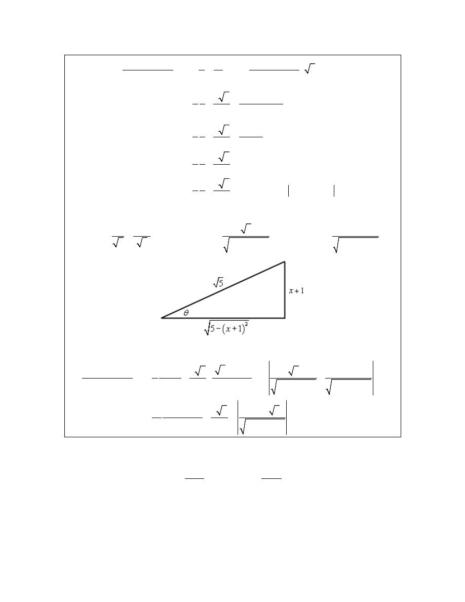
Calculus II
(
)
(
)
(
)
(
)
(
)
2
2
2
2
2
2
2
4
3
3
1
1
4
5 cos
2
4 2
5 5sin
1 1
4 5
cos
2
25
1 sin
1 1
4 5
cos
2
25
cos
1 1
4 5
sec
2
25
1 1
2 5
sec tan
ln sec
tan
2
25
x
dx
dv
d
v
x
x
d
v
d
v
d
v
c
v
θ θ
θ
θ
θ
θ
θ θ
θ
θ θ
θ
θ
θ
θ
−
= −
−
−
−
−
=
−
−
=
−
=
−
=
−
+
+
+
⌠
⌠
⌠
⌡
⌡
⌡
⌠
⌡
⌠
⌡
∫
We’ll need the following right triangle to finish this integral out.
(
)
(
)
2
2
1
5
1
sin
sec
tan
5
5
5
1
5
1
u
x
x
x
x
θ
θ
θ
+
+
=
=
=
=
− +
− +
So, going back to x’s the integral becomes,
(
)
(
)
(
)
(
)
(
)
(
)
(
)
2
2
2
2
2
2
2
2
5
1
3
1
1
2 5
5
1
ln
2 5
25
5
1
4 2
5
1
5
1
1
4
1
2 5
1
5
ln
10
25
5
1
5
1
x
x
x
dx
c
u
x
x
x
x
x
x
x
c
x
x
+
−
+
=
−
+
+
+
−
−
+
−
−
−
+
−
+
−
+ +
=
−
+
−
+
−
+
⌠
⌡
Often the following formula is needed when using the trig substitution that we used in the
previous example.
2
2
1
2
sec
tan sec
sec
1
1
m
m
m
m
d
d
m
m
θ θ
θ
θ
θ θ
−
−
−
=
+
−
−
∫
∫
Note that we’ll only need the two trig substitutions that we used here. The third trig substitution
that we used will not be needed here.
© 2007 Paul Dawkins
50
http://tutorial.math.lamar.edu/terms.aspx

Calculus II
Integration Strategy
We’ve now seen a fair number of different integration techniques and so we should probably
pause at this point and talk a little bit about a strategy to use for determining the correct technique
to use when faced with an integral.
There are a couple of points that need to be made about this strategy. First, it isn’t a hard and fast
set of rules for determining the method that should be used. It is really nothing more than a
general set of guidelines that will help us to identify techniques that may work. Some integrals
can be done in more than one way and so depending on the path you take through the strategy
you may end up with a different technique than somebody else who also went through this
strategy.
Second, while the strategy is presented as a way to identify the technique that could be used on an
integral also keep in mind that, for many integrals, it can also automatically exclude certain
techniques as well. When going through the strategy keep two lists in mind. The first list is
integration techniques that simply won’t work and the second list is techniques that look like they
might work. After going through the strategy and the second list has only one entry then that is
the technique to use. If, on the other hand, there is more than one possible technique to use we
will then have to decide on which is liable to be the best for us to use. Unfortunately there is no
way to teach which technique is the best as that usually depends upon the person and which
technique they find to be the easiest.
Third, don’t forget that many integrals can be evaluated in multiple ways and so more than one
technique may be used on it. This has already been mentioned in each of the previous points, but
is important enough to warrant a separate mention. Sometimes one technique will be
significantly easier than the others and so don’t just stop at the first technique that appears to
work. Always identify all possible techniques and then go back and determine which you feel
will be the easiest for you to use.
Next, it’s entirely possible that you will need to use more than one method to completely do an
integral. For instance a substitution may lead to using integration by parts or partial fractions
integral.
Finally, in my class I will accept any valid integration technique as a solution. As already noted
there is often more than one way to do an integral and just because I find one technique to be the
easiest doesn’t mean that you will as well. So, in my class, there is no one right way of doing an
integral. You may use any integration technique that I’ve taught you in this class or you learned
in Calculus I to evaluate integrals in this class. In other words, always take the approach that you
find to be the easiest.
Note that this final point is more geared towards my class and it’s completely possible that your
instructor may not agree with this and so be careful in applying this point if you aren’t in my
class.
Okay, let’s get on with the strategy.
© 2007 Paul Dawkins
51
http://tutorial.math.lamar.edu/terms.aspx

Calculus II
1. Simplify the integrand, if possible. This step is very important in the integration
process. Many integrals can be taken from impossible or very difficult to very easy with
a little simplification or manipulation. Don’t forget basic trig and algebraic identities as
these can often be used to simplify the integral.
We used this idea when we were looking at integrals involving trig functions. For
example consider the following integral.
2
cos x dx
∫
This integral can’t be done as is, however simply by recalling the identity,
( )
(
)
2
1
cos
1 cos 2
2
x
x
=
+
the integral becomes very easy to do.
Note that this example also shows that simplification does not necessarily mean that we’ll
write the integrand in a “simpler” form. It only means that we’ll write the integrand into
a form that we can deal with and this is often longer and/or “messier” than the original
integral.
2. See if a “simple” substitution will work. Look to see if a simple substitution can be
used instead of the often more complicated methods from Calculus II. For example
consider both of the following integrals.
2
2
1
1
x
dx
x x
dx
x
−
−
⌠
⌡
∫
The first integral can be done with partial fractions and the second could be done with a
trig substitution.
However, both could also be evaluated using the substitution
2
1
u
x
=
−
and the work
involved in the substitution would be significantly less than the work involved in either
partial fractions or trig substitution.
So, always look for quick, simple substitutions before moving on to the more
complicated Calculus II techniques.
3. Identify the type of integral. Note that any integral may fall into more than one of these
types. Because of this fact it’s usually best to go all the way through the list and identify
all possible types since one may be easier than the other and it’s entirely possible that the
easier type is listed lower in the list.
a. Is the integrand a rational expression (i.e is the integrand a polynomial divided by
a polynomial)? If so, then partial fractions may work on the integral.
b. Is the integrand a polynomial times a trig function, exponential, or logarithm? If
so, then integration by parts may work.
c. Is the integrand a product of sines and cosines, secant and tangents, or cosecants
and cotangents? If so, then the topics from the second section may work.
Likewise, don’t forget that some quotients involving these functions can also be
done using these techniques.
© 2007 Paul Dawkins
52
http://tutorial.math.lamar.edu/terms.aspx

Calculus II
d. Does the integrand involve
2
2
2
b x
a
+
,
2
2
2
b x
a
−
, or
2
2
2
a
b x
−
? If so,
then a trig substitution might work nicely.
e. Does the integrand have roots other than those listed above in it? If so, then the
substitution
( )
n
u
g x
=
might work.
f. Does the integrand have a quadratic in it? If so, then completing the square on
the quadratic might put it into a form that we can deal with.
4. Can we relate the integral to an integral we already know how to do? In other words,
can we use a substitution or manipulation to write the integrand into a form that does fit
into the forms we’ve looked at previously in this chapter.
A typical example here is the following integral.
2
cos
1 sin
x
x dx
+
∫
This integral doesn’t obviously fit into any of the forms we looked at in this chapter.
However, with the substitution
sin
u
x
=
we can reduce the integral to the form,
2
1 u du
+
∫
which is a trig substitution problem.
5. Do we need to use multiple techniques? In this step we need to ask ourselves if it is
possible that we’ll need to use multiple techniques. The example in the previous part is a
good example. Using a substitution didn’t allow us to actually do the integral. All it did
was put the integral and put it into a form that we could use a different technique on.
Don’t ever get locked into the idea that an integral will only require one step to
completely evaluate it. Many will require more than one step.
6. Try again. If everything that you’ve tried to this point doesn’t work then go back
through the process and try again. This time try a technique that that you didn’t use the
first time around.
As noted above this strategy is not a hard and fast set of rules. It is only intended to guide you
through the process of best determining how to do any given integral. Note as well that the only
place Calculus II actually arises is in the third step. Steps 1, 2 and 4 involve nothing more than
manipulation of the integrand either through direct manipulation of the integrand or by using a
substitution. The last two steps are simply ideas to think about in going through this strategy.
Many students go through this process and concentrate almost exclusively on Step 3 (after all this
is Calculus II, so it’s easy to see why they might do that….) to the exclusion of the other steps.
One very large consequence of that exclusion is that often a simple manipulation or substitution is
overlooked that could make the integral very easy to do.
Before moving on to the next section we should work a couple of quick problems illustrating a
couple of not so obvious simplifications/manipulations and a not so obvious substitution.
© 2007 Paul Dawkins
53
http://tutorial.math.lamar.edu/terms.aspx

Calculus II
Example 1
Evaluate the following integral.
4
tan
sec
x
dx
x
⌠
⌡
Solution
This integral almost falls into the form given in 3c. It is a quotient of tangent and secant and we
know that sometimes we can use the same methods for products of tangents and secants on
quotients.
The process from that
tells us that if we have even powers of secant to strip two of them
off and convert the rest to tangents. That won’t work here. We can split two secants off, but they
would be in the denominator and they won’t do us any good there. Remember that the point of
splitting them off is so they would be there for the substitution
tan
u
x
=
. That requires them to
be in the numerator. So, that won’t work and so we’ll have to find another solution method.
There are in fact two solution methods to this integral depending on how you want to go about it.
We’ll take a look at both.
Solution 1
In this solution method we could just convert everything to sines and cosines and see if that gives
us an integral we can deal with.
4
4
3
3
4
tan
sin
cos
sec
cos
sin cos
cos
1
cos
4
x
x
dx
x dx
x
x
x
x dx
u
x
u du
x
c
=
=
=
= −
= −
+
⌠
⌠
⌡
⌡
∫
∫
Note that just converting to sines and cosines won’t always work and if it does it won’t always
work this nicely. Often there will be a lot more work that would need to be done to complete the
integral.
Solution 2
This solution method goes back to dealing with secants and tangents. Let’s notice that if we had
a secant in the numerator we could just use
sec
u
x
=
as a substitution and it would be a fairly
quick and simple substitution to use. We don’t have a secant in the numerator. However we
could very easily get a secant in the numerator simply by multiplying the numerator and
denominator by secant.
4
5
5
4
4
tan
tan sec
sec
sec
sec
1
1
1
4 sec
1
cos
4
x
x
x
dx
dx
u
x
x
x
du
u
c
x
x
c
=
=
=
= −
+
= −
+
⌠
⌠
⌡
⌡
⌠
⌡
© 2007 Paul Dawkins
54
http://tutorial.math.lamar.edu/terms.aspx

Calculus II
In the previous example we saw two “simplifications” that allowed us to do the integral. The first
was using identities to rewrite the integral into terms we could deal with and the second involved
multiplying the numerator and the denominator by something to again put the integral into terms
we could deal with.
Using identities to rewrite an integral is an important “simplification” and we should not forget
about it. Integrals can often be greatly simplified or at least put into a form that can be dealt with
by using an identity.
The second “simplification” is not used as often, but does show up on occasion so again, it’s best
to not forget about it. In fact, let’s take another look at an example in which multiplying the
numerator and denominator by something will allow us to do an integral.
Example 2
Evaluate the following integral.
1
1 sin
dx
x
+
⌠
⌡
Solution
This is an integral in which if we just concentrate on the third step we won’t get anywhere. This
integral doesn’t appear to be any of the kinds of integrals that we worked in this chapter.
We can do the integral however, if we do the following,
2
1
1
1 sin
1 sin
1 sin 1 sin
1 sin
1 sin
x
dx
dx
x
x
x
x
dx
x
−
=
+
+
−
−
=
−
⌠
⌠
⌡
⌡
⌠
⌡
This does not appear to have done anything for us. However, if we now remember the first
“simplification” we looked at above we will notice that we can use an identity to rewrite the
denominator. Once we do that we can further reduce the integral into something we can deal
with.
2
2
2
1
1 sin
1 sin
cos
1
sin
1
cos
cos
cos
sec
tan sec
tan
sec
x
dx
dx
x
x
x
dx
x
x
x
x
x
x dx
x
x
c
−
=
+
=
−
=
−
=
−
+
⌠
⌠
⌡
⌡
⌠
⌡
∫
So, we’ve seen once again that multiplying the numerator and denominator by something can put
the integral into a form that we can integrate. Notice as well that this example also showed that
“simplifications” do not necessarily put an integral into a simpler form. They only put the
integral into a form that is easier to integrate.
Let’s now take a quick look at an example of a substitution that is not so obvious.
© 2007 Paul Dawkins
55
http://tutorial.math.lamar.edu/terms.aspx
Calculus II
Example 3
Evaluate the following integral.
( )
cos
x dx
∫
Solution
We introduced this example saying that the substitution was not so obvious. However, this is
really an integral that falls into the form given by 3e in our strategy above. However, many
people miss that form and so don’t think about it. So, let’s try the following substitution.
2
2
u
x
x
u
dx
u du
=
=
=
With this substitution the integral becomes,
( )
cos
2
cos
x dx
u
u du
=
∫
∫
This is now an integration by parts integral. Remember that often we will need to use more than
one technique to completely do the integral. This is a fairly simple integration by parts problem
so I’ll leave the remainder of the details to you to check.
( )
( )
( )
(
)
cos
2 cos
sin
x dx
x
x
x
c
=
+
+
∫
Before leaving this section we should also point out that there are integrals out there in the world
that just can’t be done in terms of functions that we know. Some examples of these are.
( )
( )
( )
2
2
sin
cos
cos
x
x
x
dx
x
dx
dx
dx
x
−
⌠
⌡
∫
∫
∫
e
e
That doesn’t mean that these integrals can’t be done at some level. If you go to a computer
algebra system such as
and have it do these integrals it will return the
following.
( )
( )
( )
( )
( )
( )
2
2
erf
2
2
cos
FresnelC
2
sin
Si
cos
Ci
x
x
x
dx
x
x
dx
x
x
dx
x
x
dx
π
π
π
−
=
=
=
=
⌠
⌡
∫
∫
∫
e
e
e
So it appears that these integrals can in fact be done. However this is a little misleading. Here
are the definitions of each of the functions given above.
Error Function
( )
0
2
2
erf
x
t
x
dt
π
−
=
∫
e
The Sine Integral
( )
0
sin
Si
x
t
x
dt
t
= ⌠
⌡
© 2007 Paul Dawkins
56
http://tutorial.math.lamar.edu/terms.aspx

Calculus II
The Fresnel Cosine Integral
( )
2
0
FresnelC
cos
2
x
x
t
dt
π
=
⌠
⌡
The Cosine Integral
( )
( )
0
cos
1
Ci
ln
x
t
x
x
dt
t
γ
−
= +
+ ⌠
⌡
Where
γ
is the
Note that the first three are simply defined in terms of themselves and so when we say we can
integrate them all we are really doing is renaming the integral. The fourth one is a little different
and yet it is still defined in terms of an integral that can’t be done in practice.
It will be possible to integrate every integral given in this class, but it is important to note that
there are integrals that just can’t be done. We should also note that after we look at
will be able to write down series representations of each of the integrals above.
© 2007 Paul Dawkins
57
http://tutorial.math.lamar.edu/terms.aspx

Calculus II
Improper Integrals
In this section we need to take a look at a couple of different kinds of integrals. Both of these are
examples of integrals that are called Improper Integrals.
Let’s start with the first kind of improper integrals that we’re going to take a look at.
Infinite Interval
In this kind of integral one or both of the limits of integration are infinity. In these cases the
interval of integration is said to be over an infinite interval.
Let’s take a look at an example that will also show us how we are going to deal with these
integrals.
Example 1
Evaluate the following integral.
2
1
1
dx
x
∞
⌠
⌡
Solution
This is an innocent enough looking integral. However, because infinity is not a real number we
can’t just integrate as normal and then “plug in” the infinity to get an answer.
To see how we’re going to do this integral let’s think of this as an area problem. So instead of
asking what the integral is, let’s instead ask what the area under
( )
2
1
f x
x
=
on the interval
[
)
1,
∞
is.
We still aren’t able to do this, however, let’s step back a little and instead ask what the area under
( )
f x
is on the interval
[ ]
1, t
where
1
t
>
and t is finite. This is a problem that we can do.
2
1
1
1
1
1
1
t
t
t
A
dx
x
x
t
=
= −
= −
⌠
⌡
Now, we can get the area under
( )
f x
on
[
)
1,
∞
simply by taking the limit of A
t
as t goes to
infinity.
1
lim
lim 1
1
t
t
t
A
A
t
→∞
→∞
=
=
−
=
This is then how we will do the integral itself.
2
2
1
1
1
1
1
lim
1
lim
1
lim 1
1
t
t
t
t
t
dx
dx
x
x
x
t
∞
→∞
→∞
→∞
=
=
−
=
−
=
⌠
⌠
⌡
⌡
© 2007 Paul Dawkins
58
http://tutorial.math.lamar.edu/terms.aspx

Calculus II
So, this is how we will deal with these kinds of integrals in general. We will replace the infinity
with a variable (usually t), do the integral and then take the limit of the result as t goes to infinity.
On a side note, notice that the area under a curve on an infinite interval was not infinity as we
might have suspected it to be. In fact, it was a surprisingly small number. Of course this won’t
always be the case, but it is important enough to point out that not all areas on an infinite interval
will yield infinite areas.
Let’s now get some definitions out of the way. We will call these integrals convergent if the
associated limit exists and is a finite number (i.e. it’s not plus or minus infinity) and divergent if
the associated limit either doesn’t exist or is (plus or minus) infinity.
Let’s now formalize up the method for dealing with infinite intervals. There are essentially three
cases that we’ll need to look at.
1. If
( )
t
a
f x dx
∫
exists for every
t
a
>
then,
( )
( )
lim
t
a
a
t
f x dx
f x dx
→∞
∞
=
∫
∫
provided the limit exists and is finite.
2. If
( )
b
t
f x dx
∫
exists for every
t
b
<
then,
( )
( )
lim
b
b
t
t
f x dx
f x dx
−
→−∞
∞
=
∫
∫
provided the limits exists and is finite.
3. If
( )
c
f x dx
−
∞
∫
and
( )
c
f x dx
∞
∫
are both convergent then,
( )
( )
( )
c
c
f x dx
f x dx
f x dx
−
−
∞
∞
∞
∞
=
+
∫
∫
∫
Where c is any number. Note as well that this requires BOTH of the integrals to be
convergent in order for this integral to also be convergent. If either of the two integrals is
divergent then so is this integral.
Let’s take a look at a couple more examples.
Example 2
Determine if the following integral is convergent or divergent and if it’s convergent
find its value.
1
1
dx
x
∞
⌠
⌡
Solution
So, the first thing we do is convert the integral to a limit.
1
1
1
1
lim
t
t
dx
dx
x
x
∞
→∞
=
⌠
⌠
⌡
⌡
Now, do the integral and the limit.
© 2007 Paul Dawkins
59
http://tutorial.math.lamar.edu/terms.aspx
Calculus II
( )
( )
(
)
1
1
1
lim ln
lim ln
ln1
t
t
t
dx
x
x
t
∞
→∞
→∞
=
=
−
= ∞
⌠
⌡
So, the limit is infinite and so the integral is divergent.
If we go back to thinking in terms of area notice that the area under
( )
1
x
g x
=
on the interval
[
)
1,
∞
is infinite. This is in contrast to the area under
( )
2
1
x
f x
=
which was quite small. There
really isn’t all that much difference between these two functions and yet there is a large difference
in the area under them. We can actually extend this out to the following fact.
Fact
If
0
a
>
then
1
p
a
dx
x
∞
⌠
⌡
is convergent if
1
p
>
and divergent if
1
p
≤
.
One thing to note about this fact is that it’s in essence saying that if an integrand goes to zero fast
enough then the integral will converge. How fast is fast enough? If we use this fact as a guide it
looks like integrands that go to zero faster than
1
x
goes to zero will probably converge.
Let’s take a look at a couple more examples.
Example 3
Determine if the following integral is convergent or divergent. If it is convergent
find its value.
0
1
3
dx
x
−∞
−
⌠
⌡
Solution
There really isn’t much to do with these problems once you know how to do them. We’ll convert
the integral to a limit/integral pair, evaluate the integral and then the limit.
(
)
0
0
0
1
1
lim
3
3
lim 2 3
lim
2 3
2 3
2 3
t
t
t
t
t
dx
dx
x
x
x
t
→−∞
−∞
→−∞
→−∞
=
−
−
=
−
−
=
−
+
−
= −
+ ∞
= ∞
⌠
⌠
⌡
⌡
So, the limit is infinite and so this integral is divergent.
© 2007 Paul Dawkins
60
http://tutorial.math.lamar.edu/terms.aspx

Calculus II
Example 4
Determine if the following integral is convergent or divergent. If it is convergent
find its value.
2
x
x
dx
∞
−
−∞
∫
e
Solution
In this case we’ve got infinities in both limits and so we’ll need to split the integral up into two
separate integrals. We can split the integral up at any point, so let’s choose
0
a
=
since this will
be a convenient point for the evaluation process. The integral is then,
0
0
2
2
2
x
x
x
x
dx
x
dx
x
dx
∞
∞
−
−
−
−∞
−∞
=
+
∫
∫
∫
e
e
e
We’ve now got to look at each of the individual limits.
0
0
0
2
2
2
2
lim
1
lim
2
1
1
lim
2
2
1
2
t
t
t
t
t
t
x
x
x
x
dx
x
dx
−
−
−∞
→−∞
−
→−∞
−
→−∞
=
=
−
=
− +
= −
∫
∫
e
e
e
e
So, the first integral is convergent. Note that this does NOT mean that the second integral will
also be convergent. So, let’s take a look at that one.
0
0
0
2
2
2
2
lim
1
lim
2
1
1
lim
2
2
1
2
t
t
t
t
t
t
x
x
x
x
dx
x
dx
∞
−
−
→∞
−
→∞
−
→∞
=
=
−
=
−
+
=
∫
∫
e
e
e
e
This integral is convergent and so since they are both convergent the integral we were actually
asked to deal with is also convergent and its value is,
0
0
2
2
2
1
1
0
2
2
x
x
x
x
dx
x
dx
x
dx
∞
∞
−
−
−
−∞
−∞
=
+
= − + =
∫
∫
∫
e
e
e
Example 5
Determine if the following integral is convergent or divergent. If it is convergent
find its value.
2
sin x dx
∞
−
∫
Solution
First convert to a limit.
© 2007 Paul Dawkins
61
http://tutorial.math.lamar.edu/terms.aspx

Calculus II
(
)
(
)
2
2
2
sin
lim
sin
lim
cos
lim cos 2 cos
t
t
t
t
t
x dx
x dx
x
t
∞
−
−
→∞
−
→∞
→∞
=
=
−
=
−
∫
∫
This limit doesn’t exist and so the integral is divergent.
In most examples in a Calculus II class that are worked over infinite intervals the limit either
exists or is infinite. However, there are limits that don’t exist, as the previous example showed,
so don’t forget about those.
Discontinuous Integrand
We now need to look at the second type of improper integrals that we’ll be looking at in this
section. These are integrals that have discontinuous integrands. The process here is basically the
same with one subtle difference. Here are the general cases that we’ll look at for these integrals.
1. If
( )
f x
is continuous on the interval
[
)
,
a b
and not continuous at
x
b
=
then,
( )
( )
lim
b
t
a
a
t
b
f x dx
f x dx
−
→
=
∫
∫
provided the limit exists and is finite. Note as well that we do need to use a left hand
limit here since the interval of integration is entirely on the left side of the upper limit.
2. If
( )
f x
is continuous on the interval
(
]
,
a b
and not continuous at
x
a
=
then,
( )
( )
lim
b
b
a
t
t
a
f x dx
f x dx
+
→
=
∫
∫
provided the limit exists and is finite. In this case we need to use a right hand limit here
since the interval of integration is entirely on the right side of the lower limit.
3. If
( )
f x
is not continuous at
x
c
=
where
a
c
b
< <
and
( )
c
a
f x dx
∫
and
( )
b
c
f x dx
∫
are both convergent then,
( )
( )
( )
b
c
b
a
a
c
f x dx
f x dx
f x dx
=
+
∫
∫
∫
As with the infinite interval case this requires BOTH of the integrals to be convergent in
order for this integral to also be convergent. If either of the two integrals is divergent
then so is this integral.
4. If
( )
f x
is not continuous at
x
a
=
and
x
b
=
and if
( )
c
a
f x dx
∫
and
( )
b
c
f x dx
∫
are
both convergent then,
( )
( )
( )
b
c
b
a
a
c
f x dx
f x dx
f x dx
=
+
∫
∫
∫
Where c is any number. Again, this requires BOTH of the integrals to be convergent in
order for this integral to also be convergent.
© 2007 Paul Dawkins
62
http://tutorial.math.lamar.edu/terms.aspx
Calculus II
Note that the limits in these cases really do need to be right or left handed limits. Since we will
be working inside the interval of integration we will need to make sure that we stay inside that
interval. This means that we’ll use one-sided limits to make sure we stay inside the interval.
Let’s do a couple of examples of these kinds of integrals.
Example 6
Determine if the following integral is convergent or divergent. If it is convergent
find its value.
3
0
1
3
dx
x
−
⌠
⌡
Solution
The problem point is the upper limit so we are in the first case above.
(
)
(
)
3
3
0
0
3
0
3
1
1
lim
3
3
lim
2 3
lim 2 3
2 3
2 3
t
t
t
t
t
dx
dx
x
x
x
t
−
−
−
→
→
→
=
−
−
=
−
−
=
−
−
=
⌠
⌠
⌡
⌡
The limit exists and is finite and so the integral converges and the integral’s value is
2 3
.
Example 7
Determine if the following integral is convergent or divergent. If it is convergent
find its value.
3
3
2
1
dx
x
−
⌠
⌡
Solution
This integrand is not continuous at
0
x
=
and so we’ll need to split the integral up at that point.
3
0
3
3
3
3
2
2
0
1
1
1
dx
dx
dx
x
x
x
−
−
=
+
⌠
⌠
⌠
⌡
⌡
⌡
Now we need to look at each of these integrals and see if they are convergent.
0
3
3
0
2
2
2
0
2
2
0
1
1
lim
1
lim
2
1
1
lim
2
8
t
t
t
t
t
dx
dx
x
x
x
t
−
−
−
→
−
−
→
−
→
=
=
−
=
−
+
= −∞
⌠
⌠
⌡
⌡
At this point we’re done. One of the integrals is divergent that means the integral that we were
asked to look at is divergent. We don’t even need to bother with the second integral.
© 2007 Paul Dawkins
63
http://tutorial.math.lamar.edu/terms.aspx

Calculus II
Before leaving this section let’s note that we can also have integrals that involve both of these
cases. Consider the following integral.
Example 8
Determine if the following integral is convergent or divergent. If it is convergent
find its value.
2
0
1
dx
x
∞
⌠
⌡
Solution
This is an integral over an infinite interval that also contains a discontinuous integrand. To do
this integral we’ll need to split it up into two integrals. We can split it up anywhere, but pick a
value that will be convenient for evaluation purposes.
1
2
2
2
0
0
1
1
1
1
dx
dx
dx
x
x
x
∞
∞
=
+
⌠
⌠
⌠
⌡
⌡
⌡
In order for the integral in the example to be convergent we will need BOTH of these to be
convergent. If one or both are divergent then the whole integral will also be divergent.
We know that the second integral is convergent by the fact given in the infinite interval portion
above. So, all we need to do is check the first integral.
1
1
2
2
0
0
1
0
0
1
1
lim
1
lim
1
lim
1
t
t
t
t
t
dx
dx
x
x
x
t
+
+
+
→
→
→
=
=
−
=
− +
= ∞
⌠
⌠
⌡
⌡
So, the first integral is divergent and so the whole integral is divergent.
© 2007 Paul Dawkins
64
http://tutorial.math.lamar.edu/terms.aspx

Calculus II
Comparison Test for Improper Integrals
Now that we’ve seen how to actually compute improper integrals we need to address one more
topic about them. Often we aren’t concerned with the actual value of these integrals. Instead we
might only be interested in whether the integral is convergent or divergent. Also, there will be
some integrals that we simply won’t be able to integrate and yet we would still like to know if
they converge or diverge.
To deal with this we’ve got a test for convergence or divergence that we can use to help us
answer the question of convergence for an improper integral.
We will give this test only for a sub-case of the infinite interval integral, however versions of the
test exist for the other sub-cases of the infinite interval integrals as well as integrals with
discontinuous integrands.
Comparison Test
If
( )
( )
0
f x
g x
≥
≥
on the interval
[
)
,
a
∞
then,
1. If
( )
a
f x dx
∞
∫
converges then so does
( )
a
g x dx
∞
∫
.
2. If
( )
a
g x dx
∞
∫
diverges then so does
( )
a
f x dx
∞
∫
.
Note that if you think in terms of area the Comparison Test makes a lot of sense. If
( )
f x
is
larger than
( )
g x
then the area under
( )
f x
must also be larger than the area under
( )
g x
.
So, if the area under the larger function is finite (i.e.
( )
a
f x dx
∞
∫
converges) then the area under
the smaller function must also be finite (i.e.
( )
a
g x dx
∞
∫
converges). Likewise, if the area under
the smaller function is infinite (i.e.
( )
a
g x dx
∞
∫
diverges) then the area under the larger function
must also be infinite (i.e.
( )
a
f x dx
∞
∫
diverges).
Be careful not to misuse this test. If the smaller function converges there is no reason to believe
that the larger will also converge (after all infinity is larger than a finite number…) and if the
larger function diverges there is no reason to believe that the smaller function will also diverge.
Let’s work a couple of examples using the comparison test. Note that all we’ll be able to do is
determine the convergence of the integral. We won’t be able to determine the value of the
integrals and so won’t even bother with that.
© 2007 Paul Dawkins
65
http://tutorial.math.lamar.edu/terms.aspx

Calculus II
Example 1
Determine if the following integral is convergent or divergent.
2
2
2
cos x
dx
x
∞
⌠
⌡
Solution
Let’s take a second and think about how the Comparison Test works. If this integral is
convergent then we’ll need to find a larger function that also converges on the same interval.
Likewise, if this integral is divergent then we’ll need to find a smaller function that also diverges.
So, it seems like it would be nice to have some idea as to whether the integral converges or
diverges ahead of time so we will know whether we will need to look for a larger (and
convergent) function or a smaller (and divergent) function.
To get the guess for this function let’s notice that the numerator is nice and bounded and simply
won’t get too large. Therefore, it seems likely that the denominator will determine the
convergence/divergence of this integral and we know that
2
2
1
dx
x
∞
⌠
⌡
converges since
2 1
p
= >
by the fact in the previous
section
. So let’s guess that this integral will
converge.
So we now know that we need to find a function that is larger than
2
2
cos x
x
and also converges. Making a fraction larger is actually a fairly simple process. We can either
make the numerator larger or we can make the denominator smaller. In this case we can’t do a lot
about the denominator. However we can use the fact that
2
0
cos
1
x
≤
≤
to make the numerator
larger (i.e. we’ll replace the cosine with something we know to be larger, namely 1). So,
2
2
2
cos
1
x
x
x
≤
Now, as we’ve already noted
2
2
1
dx
x
∞
⌠
⌡
converges and so by the Comparison Test we know that
2
2
2
cos x
dx
x
∞
⌠
⌡
must also converge.
Example 2
Determine if the following integral is convergent or divergent.
3
1
x
dx
x
∞
+
⌠
⌡
e
Solution
Let’s first take a guess about the convergence of this integral. As noted after the fact in the last
section about
© 2007 Paul Dawkins
66
http://tutorial.math.lamar.edu/terms.aspx

Calculus II
1
p
a
dx
x
∞
⌠
⌡
if the integrand goes to zero faster than
1
x
then the integral will probably converge. Now, we’ve
got an exponential in the denominator which is approaching infinity much faster than the x and so
it looks like this integral should probably converge.
So, we need a larger function that will also converge. In this case we can’t really make the
numerator larger and so we’ll need to make the denominator smaller in order to make the function
larger as a whole. We will need to be careful however. There are two ways to do this and only
one, in this case only one, of them will work for us.
First, notice that since the lower limit of integration is 3 we can say that
3
0
x
≥ >
and we know
that exponentials are always positive. So, the denominator is the sum of two positive terms and if
we were to drop one of them the denominator would get smaller. This would in turn make the
function larger.
The question then is which one to drop? Let’s first drop the exponential. Doing this gives,
1
1
x
x
x
<
+ e
This is a problem however, since
3
1
dx
x
∞
⌠
⌡
diverges by the
fact
. We’ve got a larger function that is divergent. This doesn’t say anything
about the smaller function. Therefore, we chose the wrong one to drop.
Let’s try it again and this time let’s drop the x.
1
1
x
x
x
x
−
<
=
+
e
e
e
Also,
(
)
3
3
3
3
lim
lim
t
x
x
t
t
t
dx
dx
∞ −
−
→∞
−
−
→∞
−
=
=
−
+
=
∫
∫
e
e
e
e
e
So,
3
x
dx
∞ −
∫
e
is convergent. Therefore, by the Comparison test
3
1
x
dx
x
∞
+
⌠
⌡
e
is also convergent.
© 2007 Paul Dawkins
67
http://tutorial.math.lamar.edu/terms.aspx

Calculus II
Example 3
Determine if the following integral is convergent or divergent.
3
1
x
dx
x
∞
−
−
⌠
⌡
e
Solution
This is very similar to the previous example with a couple of very important differences. First,
notice that the exponential now goes to zero as x increases instead of growing larger as it did in
the previous example (because of the negative in the exponent). Also note that the exponential is
now subtracted off the x instead of added onto it.
The fact that the exponential goes to zero means that this time the x in the denominator will
probably dominate the term and that means that the integral probably diverges. We will therefore
need to find a smaller function that also diverges.
Making fractions smaller is pretty much the same as making fractions larger. In this case we’ll
need to either make the numerator smaller or the denominator larger.
This is where the second change will come into play. As before we know that both x and the
exponential are positive. However, this time since we are subtracting the exponential from the x
if we were to drop the exponential the denominator will become larger and so the fraction will
become smaller. In other words,
1
1
x
x
x
−
>
− e
and we know that
3
1
dx
x
∞
⌠
⌡
diverges and so by the Comparison Test we know that
3
1
x
dx
x
∞
−
−
⌠
⌡
e
must also diverge.
Example 4
Determine if the following integral is convergent or divergent.
( )
4
1
1 3sin
2x
dx
x
∞
+
⌠
⌡
Solution
First notice that as with the first example, the numerator in this function is going to be bounded
since the sine is never larger than 1. Therefore, since the exponent on the denominator is less
than 1 we can guess that the integral will probably diverge. We will need a smaller function that
also diverges.
We know that
( )
4
0
sin
2
1
x
≤
≤
. In particular, this term is positive and so if we drop it from the
numerator the numerator will get smaller. This gives,
( )
4
1 3sin
2
1
x
x
x
+
>
and
© 2007 Paul Dawkins
68
http://tutorial.math.lamar.edu/terms.aspx

Calculus II
1
1
dx
x
∞
⌠
⌡
diverges so by the Comparison Test
( )
4
1
1 3sin
2x
dx
x
∞
+
⌠
⌡
also diverges.
Okay, we’ve seen a few examples of the Comparison Test now. However, most of them worked
pretty much the same way. All the functions were rational and all we did for most of them was
add or subtract something from the numerator or denominator to get what we want.
Let’s take a look at an example that works a little differently so we don’t get too locked into these
ideas.
Example 5
Determine if the following integral is convergent or divergent.
1
x
dx
x
∞ −
⌠
⌡
e
Solution
Normally, the presence of just an x in the denominator would lead us to guess divergent for this
integral. However, the exponential in the numerator will approach zero so fast that instead we’ll
need to guess that this integral converges.
To get a larger function we’ll use the fact that we know from the limits of integration that
1
x
>
.
This means that if we just replace the x in the denominator with 1 (which is always smaller than
x) we will make the denominator smaller and so the function will get larger.
1
x
x
x
x
−
−
−
<
=
e
e
e
and we can show that
1
x
dx
∞ −
∫
e
converges. In fact, we’ve already done this for a lower limit of 3 and changing that to a 1 won’t
change the convergence of the integral. Therefore, by the Comparison Test
1
x
dx
x
∞ −
⌠
⌡
e
also converges.
We should also really work an example that doesn’t involve a rational function since there is no
reason to assume that we’ll always be working with rational functions.
Example 6
Determine if the following integral is convergent or divergent.
1
2
x
dx
∞ −
∫
e
Solution
We know that exponentials with negative exponents die down to zero very fast so it makes sense
to guess that this integral will be convergent. We need a larger function, but this time we don’t
© 2007 Paul Dawkins
69
http://tutorial.math.lamar.edu/terms.aspx
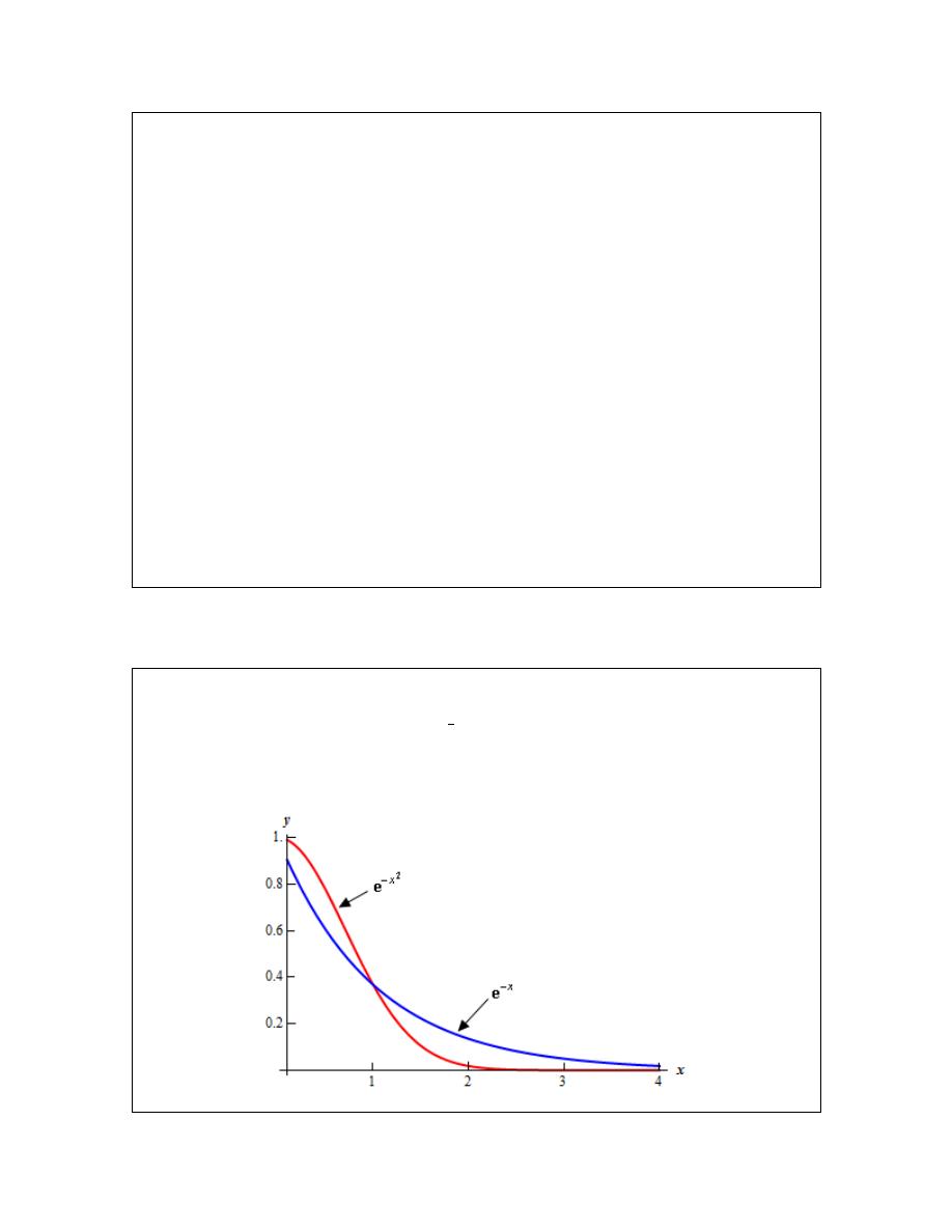
Calculus II
have a fraction to work with so we’ll need to do something different.
We’ll take advantage of the fact that
x
−
e
is a decreasing function. This means that
1
2
1
2
x
x
x
x
−
−
>
⇒
<
e
e
In other words, plug in a larger number and the function gets smaller.
From the limits of integration we know that
1
x
>
and this means that if we square x it will get
larger. Or,
2
provided 1
x
x
x
>
>
Note that we can only say this since
1
x
>
. This won’t be true if
1
x
≤
! We can now use the fact
that
x
−
e
is a decreasing function to get,
2
x
x
−
−
<
e
e
So,
x
−
e
is a larger function than
2
x
−
e
and we know that
1
x
dx
∞ −
∫
e
converges so by the Comparison Test we also know that
1
2
x
dx
∞ −
∫
e
is convergent.
The last two examples made use of the fact that
1
x
>
. Let’s take a look at an example to see
how do we would have to go about these if the lower limit had been smaller than 1.
Example 7
Determine if the following integral is convergent or divergent.
1
2
2
x
dx
∞ −
∫
e
Solution
First, we need to note that
2
x
x
−
−
≤
e
e
is only true on the interval
[
)
1,
∞
as is illustrated in the
graph below.
© 2007 Paul Dawkins
70
http://tutorial.math.lamar.edu/terms.aspx

Calculus II
So, we can’t just proceed as we did in the previous example with the Comparison Test on the
interval
[
)
1
2
,
∞
. However, this isn’t the problem it might at first appear to be. We can always
write the integral as follows,
1
1
2
2
1
1
1
2
2
2
2
0.28554
x
x
x
x
dx
dx
dx
dx
∞
∞
−
−
−
∞ −
=
+
=
+
∫
∫
∫
∫
e
e
e
e
to get the value of the first integral. Now, if the second integral converges
it will have a finite value and so the sum of two finite values will also be finite and so the original
integral will converge. Likewise, if the second integral diverges it will either be infinite or not
have a value at all and adding a finite number onto this will not all of a sudden make it finite or
exist and so the original integral will diverge. Therefore, this integral will converge or diverge
depending only on the convergence of the second integral.
As we saw in Example 6 the second integral does converge and so the whole integral must also
converge.
As we saw in this example, if we need to, we can split the integral up into one that doesn’t
involve any problems and can be computed and one that may contain a problem that we can use
the Comparison Test on to determine its convergence.
© 2007 Paul Dawkins
71
http://tutorial.math.lamar.edu/terms.aspx
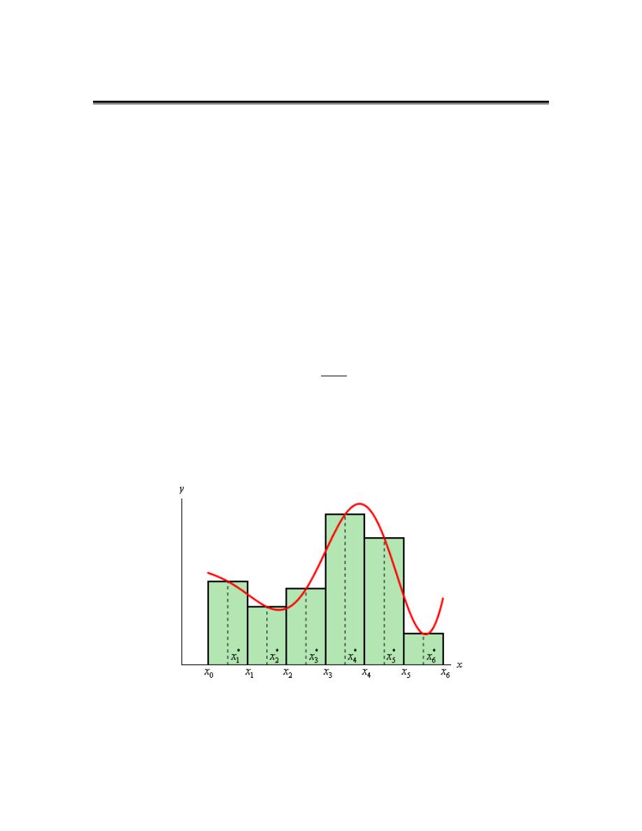
Calculus II
Approximating Definite Integrals
In this chapter we’ve spent quite a bit of time on computing the values of integrals. However, not
all integrals can be computed. A perfect example is the following definite integral.
2
0
2
x
dx
∫
e
We now need to talk a little bit about estimating values of definite integrals. We will look at
three different methods, although one should already be familiar to you from your Calculus I
days. We will develop all three methods for estimating
( )
b
a
f x dx
∫
by thinking of the integral as an area problem and using known shapes to estimate the area under
the curve.
Let’s get first develop the methods and then we’ll try to estimate the integral shown above.
Midpoint Rule
This is the rule that should be somewhat familiar to you. We will divide the interval
[ ]
,
a b
into n
subintervals of equal width,
b a
x
n
−
∆ =
We will denote each of the intervals as follows,
[
] [
]
[
]
0
1
1
2
1
0
,
,
,
,
,
,
where
and
n
n
n
x x
x x
x
x
x
a
x
b
−
=
=
Then for each interval let
*
i
x
be the midpoint of the interval. We then sketch in rectangles for
each subinterval with a height of
( )
*
i
f x
. Here is a graph showing the set up using
6
n
=
.
We can easily find the area for each of these rectangles and so for a general n we get that,
( )
( )
( )
( )
*
*
*
1
2
b
n
a
f x dx
x f x
x f x
x f x
≈ ∆
+ ∆
+ + ∆
∫
Or, upon factoring out a
x
∆
we get the general Midpoint Rule.
© 2007 Paul Dawkins
72
http://tutorial.math.lamar.edu/terms.aspx
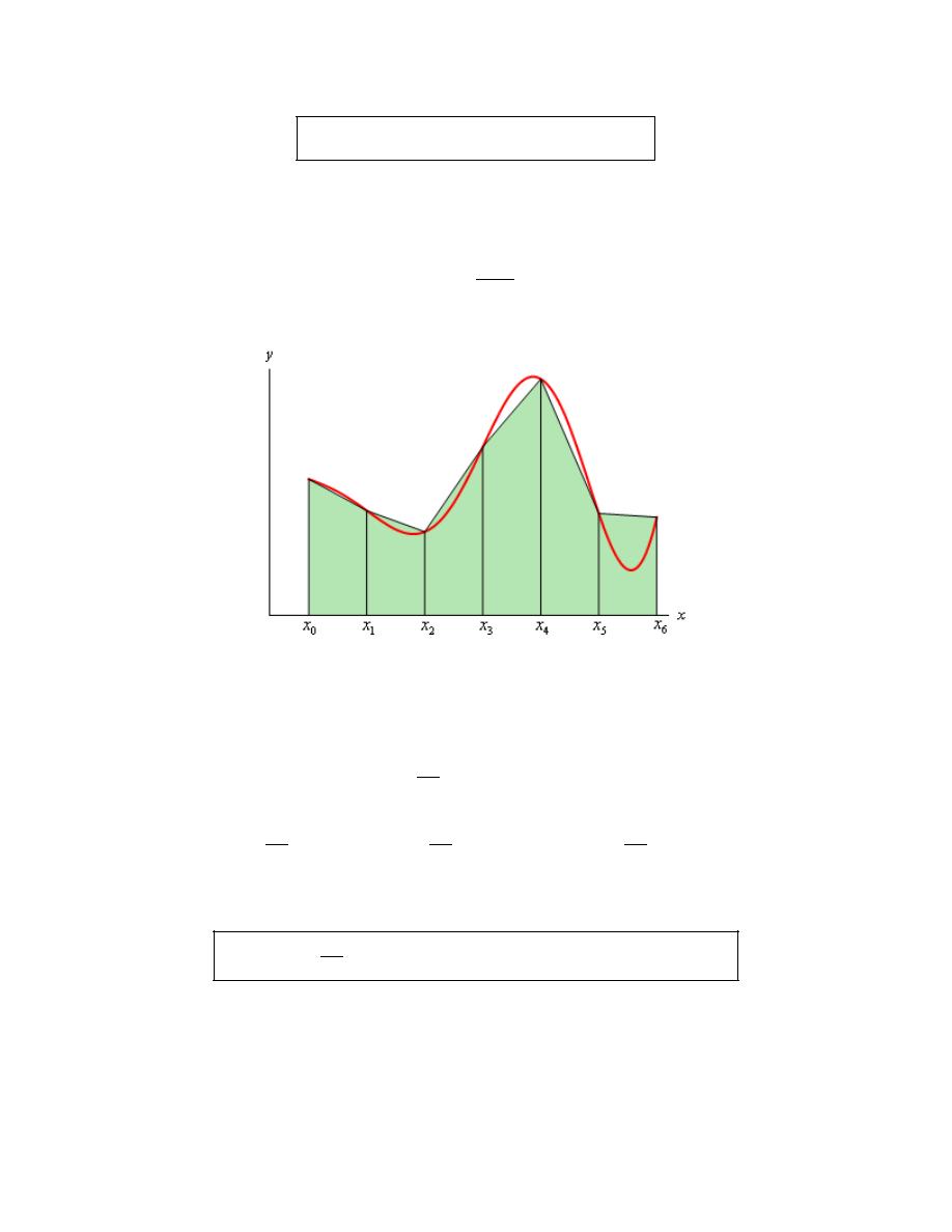
Calculus II
( )
( ) ( )
( )
*
*
*
1
2
b
n
a
f x dx
x f x
f x
f x
≈ ∆
+
+ +
∫
Trapezoid Rule
For this rule we will do the same set up as for the Midpoint Rule. We will break up the interval
[ ]
,
a b
into n subintervals of width,
b a
x
n
−
∆ =
Then on each subinterval we will approximate the function with a straight line that is equal to the
function values at either endpoint of the interval. Here is a sketch of this case for
6
n
=
.
Each of these objects is a trapezoid (hence the rule’s name…) and as we can see some of them do
a very good job of approximating the actual area under the curve and others don’t do such a good
job.
The area of the trapezoid in the interval
[
]
1
,
i
i
x
x
−
is given by,
( )
( )
(
)
1
2
i
i
i
x
A
f x
f x
−
∆
=
+
So, if we use n subintervals the integral is approximately,
( )
( )
( )
(
)
( )
( )
(
)
( )
( )
(
)
0
1
1
2
1
2
2
2
b
n
n
a
x
x
x
f x dx
f x
f x
f x
f x
f x
f x
−
∆
∆
∆
≈
+
+
+
+ +
+
∫
Upon doing a little simplification we arrive at the general Trapezoid Rule.
( )
( )
( )
( )
( )
( )
0
1
2
1
2
2
2
2
b
n
n
a
x
f x dx
f x
f x
f x
f x
f x
−
∆
≈
+
+
+ +
+
∫
Note that all the function evaluations, with the exception of the first and last, are multiplied by 2.
© 2007 Paul Dawkins
73
http://tutorial.math.lamar.edu/terms.aspx
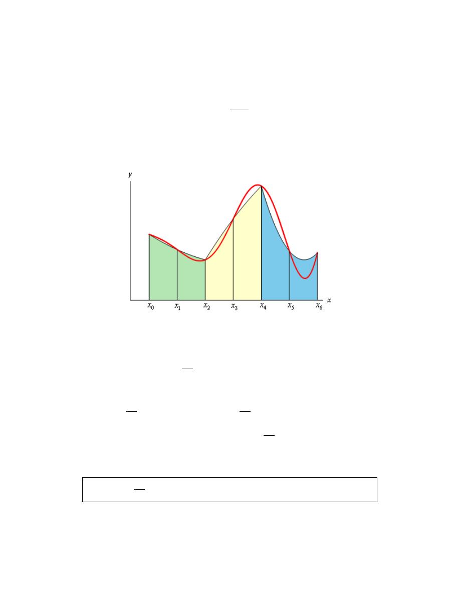
Calculus II
Simpson’s Rule
This is the final method we’re going to take a look at and in this case we will again divide up the
interval
[ ]
,
a b
into n subintervals. However unlike the previous two methods we need to require
that n be even. The reason for this will be evident in a bit. The width of each subinterval is,
b a
x
n
−
∆ =
In the Trapezoid Rule we approximated the curve with a straight line. For Simpson’s Rule we are
going to approximate the function with a quadratic and we’re going to require that the quadratic
agree with three of the points from our subintervals. Below is a sketch of this using
6
n
=
. Each
of the approximations is colored differently so we can see how they actually work.
Notice that each approximation actually covers two of the subintervals. This is the reason for
requiring n to be even. Some of the approximations look more like a line than a quadratic, but
they really are quadratics. Also note that some of the approximations do a better job than others.
It can be shown that the area under the approximation on the intervals
[
]
1
,
i
i
x
x
−
and
[
]
1
,
i
i
x x
+
is,
( )
( )
( )
(
)
1
1
4
3
i
i
i
i
x
A
f x
f x
f x
−
+
∆
=
+
+
If we use n subintervals the integral is then approximately,
( )
( )
( )
( )
(
)
( )
( )
( )
(
)
(
)
( )
( )
(
)
0
1
2
2
3
4
2
1
4
4
3
3
4
3
b
a
n
n
n
x
x
f x dx
f x
f x
f x
f x
f x
f x
x
f x
f x
f x
−
−
∆
∆
≈
+
+
+
+
+
∆
+ +
+
+
∫
Upon simplifying we arrive at the general Simpson’s Rule.
( )
( )
( )
( )
(
)
( )
( )
0
1
2
2
1
4
2
2
4
3
b
n
n
n
a
x
f x dx
f x
f x
f x
f x
f x
f x
−
−
∆
≈
+
+
+ +
+
+
∫
© 2007 Paul Dawkins
74
http://tutorial.math.lamar.edu/terms.aspx

Calculus II
In this case notice that all the function evaluations at points with odd subscripts are multiplied by
4 and all the function evaluations at points with even subscripts (except for the first and last) are
multiplied by 2. If you can remember this, this is a fairly easy rule to remember.
Okay, it’s time to work an example and see how these rules work.
Example 1
Using
4
n
=
and all three rules to approximate the value of the following integral.
2
0
2
x
dx
∫
e
Solution
First, for reference purposes, Maple gives the following value for this integral.
2
0
2
16.45262776
x
dx
=
∫
e
In each case the width of the subintervals will be,
2 0
1
4
2
x
−
∆ =
=
and so the subintervals will be,
[
] [
] [
] [
]
0, 0.5 , 0.5, 1 , 1, 1.5 , 1.5, 2
Let’s go through each of the methods.
Midpoint Rule
(
)
(
)
(
)
(
)
(
)
2
2
2
2
2
0.25
0.75
1.25
1.75
0
2
1
14.48561253
2
x
dx
≈
+
+
+
=
∫
e
e
e
e
e
Remember that we evaluate at the midpoints of each of the subintervals here! The Midpoint Rule
has an error of 1.96701523.
Trapezoid Rule
( )
( )
( )
( )
( )
(
)
2
2
2
2
2
2
0
0.5
1
1.5
2
0
2
1 2
2
2
2
20.64455905
2
x
dx
≈
+
+
+
+
=
∫
e
e
e
e
e
e
The Trapezoid Rule has an error of 4.19193129
Simpson’s Rule
( )
( )
( )
( )
( )
(
)
2
2
2
2
2
2
0
0.5
1
1.5
2
0
2
1 2
4
2
4
17.35362645
3
x
dx
≈
+
+
+
+
=
∫
e
e
e
e
e
e
The Simpson’s Rule has an error of 0.90099869.
None of the estimations in the previous example are all that good. The best approximation in this
case is from the Simpson’s Rule and yet it still had an error of almost 1. To get a better
estimation we would need to use a larger n. So, for completeness sake here are the estimates for
some larger value of n.
© 2007 Paul Dawkins
75
http://tutorial.math.lamar.edu/terms.aspx
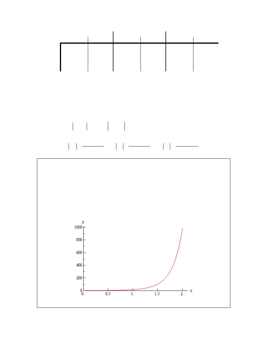
Calculus II
Midpoint
Trapezoid
Simpson’s
n
Approx.
Error
Approx.
Error
Approx.
Error
8
15.9056767 0.5469511 17.5650858 1.1124580 16.5385947 0.0859669
16
16.3118539 0.1407739 16.7353812 0.2827535 16.4588131 0.0061853
32
16.4171709 0.0354568 16.5236176 0.0709898 16.4530297 0.0004019
64
16.4437469 0.0088809 16.4703942 0.0177665 16.4526531 0.0000254
128 16.4504065 0.0022212 16.4570706 0.0044428 16.4526294 0.0000016
In this case we were able to determine the error for each estimate because we could get our hands
on the exact value. Often this won’t be the case and so we’d next like to look at error bounds for
each estimate.
These bounds will give the largest possible error in the estimate, but it should also be pointed out
that the actual error may be significantly smaller than the bound. The bound is only there so we
can say that we know the actual error will be less than the bound.
So, suppose that
( )
f
x
K
′′
≤
and
( )
( )
4
f
x
M
≤
for
a
x
b
≤ ≤
then if E
M
, E
T
, and E
S
are the
actual errors for the Midpoint, Trapezoid and Simpson’s Rule we have the following bounds,
(
)
(
)
(
)
3
3
5
2
2
4
24
12
180
M
T
S
K b a
K b a
M b a
E
E
E
n
n
n
−
−
−
≤
≤
≤
Example 2
Determine the error bounds for the estimations in the last example.
Solution
We already know that
4
n
=
,
0
a
=
, and
2
b
=
so we just need to compute K (the largest value
of the second derivative) and M (the largest value of the fourth derivative). This means that we’ll
need the second and fourth derivative of f(x).
( )
(
)
( )
( )
(
)
2
4
2
4
2
2
2
1 2
4
3 12
4
x
x
f
x
x
f
x
x
x
′′
=
+
=
+
+
e
e
Here is a graph of the second derivative.
Here is a graph of the fourth derivative.
© 2007 Paul Dawkins
76
http://tutorial.math.lamar.edu/terms.aspx
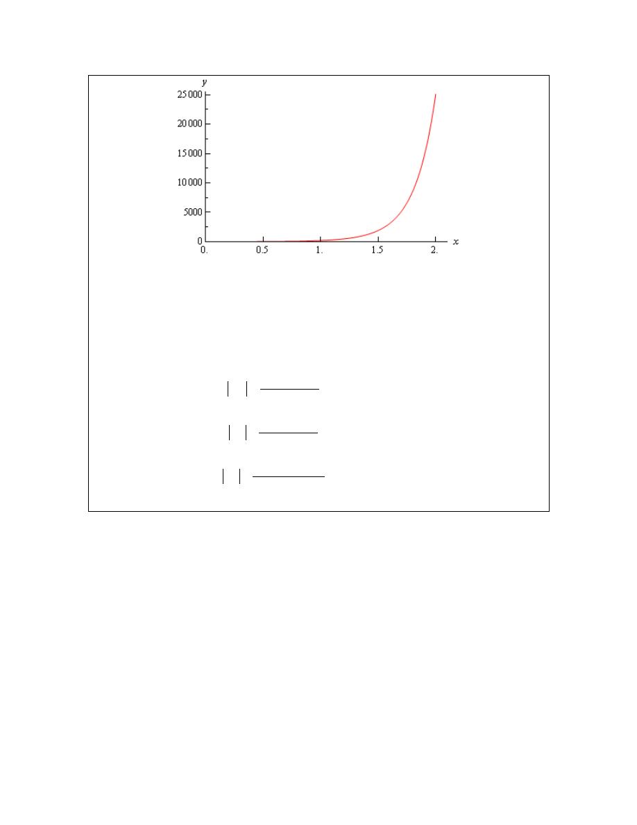
Calculus II
So, from these graphs it’s clear that the largest value of both of these are at
2
x
=
. So,
( )
( )
( )
4
2
982.76667
983
2
25115.14901
25116
f
K
f
M
′′
=
⇒
=
=
⇒
=
We rounded to make the computations simpler.
Here are the bounds for each rule.
(
)
( )
3
2
983 2 0
20.4791666667
24 4
M
E
−
≤
=
(
)
( )
3
2
983 2 0
40.9583333333
12 4
T
E
−
≤
=
(
)
( )
5
4
25116 2 0
17.4416666667
180 4
S
E
−
≤
=
In each case we can see that the errors are significantly smaller than the actual bounds.
© 2007 Paul Dawkins
77
http://tutorial.math.lamar.edu/terms.aspx

Calculus II
© 2007 Paul Dawkins
78
http://tutorial.math.lamar.edu/terms.aspx