
CALCULUS II
Solutions to Practice Problems
Applications of Integrals
Paul Dawkins
Calculus II
© 2007 Paul Dawkins
i
http://tutorial.math.lamar.edu/terms.aspx
Table of Contents
Preface ............................................................................................................................................ 1
Applications of Integrals ............................................................................................................... 1
Arc Length ................................................................................................................................................. 1
Surface Area ............................................................................................................................................... 8
Center of Mass ..........................................................................................................................................16
Hydrostatic Pressure and Force .................................................................................................................19
Probability .................................................................................................................................................30
Preface
Here are the solutions to the practice problems for my Calculus II notes. Some solutions will have more
or less detail than other solutions. As the difficulty level of the problems increases less detail will go into
the basics of the solution under the assumption that if you’ve reached the level of working the harder
problems then you will probably already understand the basics fairly well and won’t need all the
explanation.
This document was written with presentation on the web in mind. On the web most solutions are broken
down into steps and many of the steps have hints. Each hint on the web is given as a popup however in
this document they are listed prior to each step. Also, on the web each step can be viewed individually by
clicking on links while in this document they are all showing. Also, there are liable to be some formatting
parts in this document intended for help in generating the web pages that haven’t been removed here.
These issues may make the solutions a little difficult to follow at times, but they should still be readable.
Applications of Integrals
Arc Length
1. Set up, but do not evaluate, an integral for the length of
2
y
x
=
+
,
1
7
x
≤ ≤
using,
(a)
2
1
dy
ds
dx
dx
=
+
(b)
2
1
dx
ds
dy
dy
=
+
Calculus II
© 2007 Paul Dawkins
2
http://tutorial.math.lamar.edu/terms.aspx
(a)
2
1
dy
ds
dx
dx
=
+
Step 1
We’ll need the derivative of the function first.
(
)
(
)
1
2
1
2
1
1
2
2
2
2
dy
x
dx
x
−
=
+
=
+
Step 2
Plugging this into the formula for ds gives,
(
)
(
)
(
)
2
2
1
2
1
1
4
9
1
1
1
4
2
4
2
2
2
dy
x
ds
dx
dx
dx
dx
dx
x
x
x
+
=
+
=
+
=
+
=
+
+
+
Step 3
All we need to do now is set up the integral for the arc length. Also note that we have a dx in the formula
for ds and so we know that we need x limits of integration which we’ve been given in the problem
statement.
7
1
4
9
4
8
x
L
ds
dx
x
+
=
=
+
⌠
⌡
∫
(b)
2
1
dx
ds
dy
dy
=
+
Step 1
In this case we first need to solve the function for x so we can compute the derivative in the ds.
2
2
2
y
x
x
y
=
+
→
=
−
The derivative of this is,
2
dx
y
dy
=
Step 2
Plugging this into the formula for ds gives,
[ ]
2
2
2
1
1
2
1 4
dx
ds
dy
y
dy
y dy
dy
=
+
=
+
=
+
Calculus II
© 2007 Paul Dawkins
3
http://tutorial.math.lamar.edu/terms.aspx
Step 3
Next, note that the ds has a dy in it and so we’ll need y limits of integration.
We are only given x limits in the problem statement. However, we can plug these into the function we
were given in the problem statement to convert them to y limits. Doing this gives,
1:
3
7 :
9
3
x
y
x
y
=
=
=
=
=
So, the corresponding y limits are :
3
3
y
≤ ≤
.
Step 4
Finally, all we need to do is set up the integral.
3
2
3
1 4
L
ds
y dy
=
=
+
∫
∫
2. Set up, but do not evaluate, an integral for the length of
( )
cos
x
y
=
,
1
2
0
x
≤ ≤
using,
(a)
2
1
dy
ds
dx
dx
=
+
(b)
2
1
dx
ds
dy
dy
=
+
(a)
2
1
dy
ds
dx
dx
=
+
Step 1
In this case we first need to solve the function for y so we can compute the derivative in the ds.
( )
( )
( )
1
cos
cos
arccos
x
y
y
x
x
−
=
→
=
=
Which notation you use for the inverse tangent is not important since it will be “disappearing” once we
take the derivative.
Speaking of which, here is the derivative of the function.
2
1
1
dy
dx
x
= −
−
Step 2
Plugging this into the formula for ds gives,
Calculus II
© 2007 Paul Dawkins
4
http://tutorial.math.lamar.edu/terms.aspx
2
2
2
2
2
2
1
1
2
1
1
1
1
1
1
dy
x
ds
dx
dx
dx
dx
dx
x
x
x
−
=
+
=
+ −
=
+
=
−
−
−
Step 3
All we need to do now is set up the integral for the arc length. Also note that we have a dx in the formula
for ds and so we know that we need x limits of integration which we’ve been given in the problem
statement.
1
2
2
2
0
2
1
x
L
ds
dx
x
−
=
=
−
⌠
⌡
∫
(b)
2
1
dx
ds
dy
dy
=
+
Step 1
We’ll need the derivative of the function first.
( )
sin
dx
y
dy
= −
Step 2
Plugging this into the formula for ds gives,
( )
( )
2
2
2
1
1
sin
1 sin
dx
ds
dy
y
dy
y dy
dy
=
+
=
+ −
=
+
Step 3
Next, note that the ds has a dy in it and so we’ll need y limits of integration.
We are only given x limits in the problem statement. However, in part (a) we solved the function for y to
get,
( )
( )
1
cos
arccos
y
x
x
−
=
=
and all we need to do is plug x limits we were given into this to convert them to y limits. Doing this
gives,
( )
( )
1
1
0 :
cos
0
arccos 0
2
1
1
1
:
cos
arccos
2
2
2
3
x
y
x
y
π
π
−
−
=
=
=
=
=
=
=
=
Calculus II
© 2007 Paul Dawkins
5
http://tutorial.math.lamar.edu/terms.aspx
So, the corresponding y limits are :
3
2
y
π
π
≤ ≤
.
Note that we used both notations for the inverse cosine here but you only need to use the one you are
comfortable with. Also, recall that we know that the range of the inverse cosine function is,
( )
1
0
cos
x
π
−
≤
≤
Therefore, there is only one possible value of y that we can get out of each value of x.
Step 4
Finally, all we need to do is set up the integral.
( )
2
2
3
1 sin
L
ds
y dy
π
π
=
=
+
∫
∫
3. Determine the length of
(
)
3
2
7 6
y
x
=
+
,
189
875
y
≤ ≤
.
Step 1
Since we are not told which ds to use we will have to decide which one to use. In this case the function is
set up to use the ds in terms of x. Note as well that if we solve the function for x (which we’d need to do
in order to use the ds that is in terms of y) we would still have a fractional exponent and the derivative
will not work out as nice once we plug it into the ds formula.
So, let’s take the derivative of the given function and plug into the ds formula.
(
)
1
2
21
6
2
dy
x
dx
=
+
(
)
(
)
1
2
2
2
21
441
1
1
6
1
6
2
4
2650
441
1
2650 441
4
4
2
dy
ds
dx
x
dx
x dx
dx
x dx
x dx
=
+
=
+
+
=
+
+
=
+
=
+
We did a little simplification that may or may not make the integration easier. That will probably depend
upon the person doing the integration and just what they find the easiest to deal with. The point is there
are several forms of the ds that we could use here. All will give the same answer.
Step 2
Next we need to deal with the limits for the integral. The ds that we choose to use in the first step has a
dx in it and that means that we’ll need x limits for our integral. We, however, were given y limits in the
problem statement. This means we’ll need to convert those to x’s before proceeding with the integral.
Calculus II
© 2007 Paul Dawkins
6
http://tutorial.math.lamar.edu/terms.aspx
To do convert these all we need to do is plug them into the function we were given in the problem
statement and solve for the corresponding x. Doing this gives,
(
)
(
)
3
2
2
3
3
2
2
3
189 :
189
7 6
6
27
9
3
875 :
875
7 6
6
125
25
19
y
x
x
x
y
x
x
x
=
=
+
→
+ =
=
→
=
=
=
+
→
+ =
=
→
=
So, the corresponding ranges of x’s is :
3
19
x
≤ ≤
.
Step 3
The integral giving the arc length is then,
19
1
2
3
2650 441
L
ds
x dx
=
=
+
∫
∫
Step 4
Finally all we need to do is evaluate the integral. In this case all we need to do is use a quick Calc I
substitution. We’ll leave most of the integration details to you to verify.
The arc length of the curve is,
(
)
(
)
3
3
3
2
2
2
19
19
1
1
1
2
1323
1323
3
3
2650
441
2650
441
11029
3973
686.1904
L
x dx
x
=
+
=
+
=
−
=
∫
4. Determine the length of
(
)
2
4 3
x
y
=
+
,
1
4
y
≤ ≤
.
Step 1
Since we are not told which ds to use we will have to decide which one to use. In this case the function is
set up to use the ds in terms of y.
If we were to solve the function for y (which we’d need to do in order to use the ds that is in terms of x)
we would put a square root into the function and those can be difficult to deal with in arc length problems.
So, let’s take the derivative of the given function and plug into the ds formula.
(
)
8 3
dx
y
dy
=
+
(
)
(
)
2
2
2
1
1
8 3
1 64 3
dx
ds
dy
y
dy
y
dy
dy
=
+
=
+
+
=
+
+
Note that we did not square out the term under the root. Doing that would greatly complicate the
integration process so we’ll need to leave it as it is.
Calculus II
© 2007 Paul Dawkins
7
http://tutorial.math.lamar.edu/terms.aspx
Step 2
In this case we don’t need to anything special to get the limits for the integral. Our choice of ds contains
a dy which means we need y limits for the integral and nicely enough that is what we were given in the
problem statement.
So, the integral giving the arc length is,
(
)
4
2
1
1 64 3
L
ds
y
dy
=
=
+
+
∫
∫
Step 3
Finally all we need to do is evaluate the integral. In this case all we need to do is use a trig substitution.
We’ll not be putting a lot of explanation into the integration work so if you need a little refresher on trig
substitutions you should go back to that section and work a few practice problems.
The substitution we’ll need is,
2
1
1
8
8
3
tan
sec
y
dy
d
θ
θ θ
+ =
→
=
In order to properly deal with the square root we’ll need to convert the y limits to
θ
limits. Here is that
work.
( )
( )
1
1
8
1
1
8
1:
4
tan
tan
32
tan
32
1.5396
4 :
7
tan
tan
56
tan
56
1.5529
y
y
θ
θ
θ
θ
θ
θ
−
−
=
=
→
=
→
=
=
=
=
→
=
→
=
=
Now let’s deal with the square root.
(
)
(
)
2
2
2
2
1
8
1 64 3
1 64
tan
1 tan
sec
sec
y
θ
θ
θ
θ
+
+
=
+
=
+
=
=
From the work above we know that
θ
is in the range
1.5396
1.5529
θ
≤ ≤
. This is in the first and
fourth quadrants and cosine (and hence secant) is positive in this range. So,
(
)
2
1 64 3
sec
y
θ
+
+
=
Putting all of this together gives,
(
)
4
1.5529
2
3
1
8
1
1.5396
1 64 3
sec
L
y
dy
d
θ θ
=
+
+
=
∫
∫
Evaluating the integral gives,
(
)
(
)
4
1.5529
2
1
16
1.5396
1
1 64 3
tan sec
ln tan
sec
130.9570
L
y
dy
θ
θ
θ
θ
=
+
+
=
+
+
=
∫

Calculus II
© 2007 Paul Dawkins
8
http://tutorial.math.lamar.edu/terms.aspx
Note that if you used more decimal places than four here (the standard number of decimal places that we
tend to use for these problems) you may have gotten a slightly different answer. Using a computer to get
an “exact” answer gives 132.03497085.
These kinds of different answers can be a real issues with these kinds of problems and illustrates the
potential problems if you round numbers too much.
Of course, there is also the problem of often not knowing just how many decimal places are needed to get
an “accurate” answer. In many cases 4 decimal places is sufficient but there are cases (such as this one)
in which that is not enough. Often the best bet is to simply use as many decimal places as you can to
have the best chance of getting an “accurate” answer.
Surface Area
1. Set up, but do not evaluate, an integral for the surface area of the object obtained by rotating
5
x
y
=
+
,
5
3
x
≤ ≤
about the y-axis using,
(a)
2
1
dy
ds
dx
dx
=
+
(b)
2
1
dx
ds
dy
dy
=
+
(a)
2
1
dy
ds
dx
dx
=
+
Step 1
In this case we first need to solve the function for y so we can compute the derivative in the ds.
2
5
5
x
y
y
x
=
+
→
=
−
The derivative of this is,
2
dy
x
dx
=
Step 2
Plugging this into the formula for ds gives,
[ ]
2
2
2
1
1
2
1 4
dy
ds
dx
x
dx
x dx
dx
=
+
=
+
=
+
Calculus II
© 2007 Paul Dawkins
9
http://tutorial.math.lamar.edu/terms.aspx
Step 3
Finally, all we need to do is set up the integral. Also note that we have a dx in the formula for ds and so
we know that we need x limits of integration which we’ve been given in the problem statement.
3
2
5
2
2
1 4
L
x ds
x
x dx
π
π
=
=
+
∫
∫
Be careful with the formula! Remember that the variable in the integral is always opposite the axis of
rotation. In this case we rotated about the y-axis and so we needed an x in the integral.
As an aside, note that the ds we chose to use here is technically immaterial. Realistically however, one ds
may be easier than the other to work with. Determining which might be easier comes with experience
and in many cases simply trying both to see which is easier.
(b)
2
1
dx
ds
dy
dy
=
+
Step 1
We’ll need the derivative of the function first.
(
)
(
)
1
2
1
2
1
1
5
2
2
5
dx
y
dy
y
−
=
+
=
+
Step 2
Plugging this into the formula for ds gives,
(
)
(
)
(
)
2
2
1
2
1
1
4
21
1
1
1
4
5
4
5
2
5
dx
y
ds
dy
dy
dy
dy
dy
y
y
y
+
=
+
=
+
=
+
=
+
+
+
Step 3
Next, note that the ds has a dy in it and so we’ll need y limits of integration.
We are only given x limits in the problem statement. However, we can plug these into the function we
derived in Step 1 of the first part to convert them to y limits. Doing this gives,
5 :
0
3 :
4
x
y
x
y
=
=
=
=
So, the corresponding y limits are :
0
4
y
≤ ≤
.
Step 4
Finally, all we need to do is set up the integral.
Calculus II
© 2007 Paul Dawkins
10
http://tutorial.math.lamar.edu/terms.aspx
(
)
(
)
4
4
0
0
4
4
0
0
4
21
4
21
2
2
2
5
4
5
4
5
4
21
2
5
4
21
2
5
y
y
L
xds
x
dy
y
dy
y
y
y
y
dy
y
dy
y
π
π
π
π
π
+
+
=
=
=
+
+
+
+
=
+
=
+
+
⌠
⌠
⌡
⌡
⌠
⌡
∫
∫
Be careful with the formula! Remember that the variable in the integral is always opposite the axis of
rotation. In this case we rotated about the y-axis and so we needed an x in the integral.
Note that with the ds we were told to use for this part we had a dy in the final integral and that means that
all the variables in the integral need to be y’s. This means that the x from the formula needs to be
converted into y’s as well. Luckily this is easy enough to do since we were given the formula for x in
terms of y in the problem statement.
Finally, make sure you simplify these as much as possible as we did here. Had we not taken the square
root of the numerator and denominator of the rational expression we would not have seen the cancelation
that can happen there. Without that cancelation the integral would be much more difficult to do!
As an aside, note that the ds we chose to use here is technically immaterial. Realistically however, one ds
may be easier than the other to work with. Determining which might be easier comes with experience
and in many cases simply trying both to see which is easier.
2. Set up, but do not evaluate, an integral for the surface area of the object obtained by rotating
( )
sin 2
y
x
=
,
8
0
x
π
≤ ≤
about the x-axis using,
(a)
2
1
dy
ds
dx
dx
=
+
(b)
2
1
dx
ds
dy
dy
=
+
(a)
2
1
dy
ds
dx
dx
=
+
Step 1
We’ll need the derivative of the function first.
( )
2 cos 2
dy
x
dx
=
Step 2
Plugging this into the formula for ds gives,
Calculus II
© 2007 Paul Dawkins
11
http://tutorial.math.lamar.edu/terms.aspx
( )
( )
2
2
2
1
1
2 cos 2
1 4 cos
2
dy
ds
dx
x
dx
x dx
dx
=
+
=
+
=
+
Step 3
Finally, all we need to do is set up the integral. Also note that we have a dx in the formula for ds and so
we know that we need x limits of integration which we’ve been given in the problem statement.
( )
( )
( )
8
8
2
2
0
0
2
2
1 4 cos
2
2 sin 2
1 4 cos
2
L
y ds
y
x dx
x
x dx
π
π
π
π
π
=
=
+
=
+
∫
∫
∫
Be careful with the formula! Remember that the variable in the integral is always opposite the axis of
rotation. In this case we rotated about the x-axis and so we needed a y in the integral.
Note that with the ds we were told to use for this part we had a dx in the final integral and that means that
all the variables in the integral need to be x’s. This means that the y from the formula needs to be
converted into x’s as well. Luckily this is easy enough to do since we were given the formula for y in
terms of x in the problem statement.
As an aside, note that the ds we chose to use here is technically immaterial. Realistically however, one ds
may be easier than the other to work with. Determining which might be easier comes with experience
and in many cases simply trying both to see which is easier.
(b)
2
1
dx
ds
dy
dy
=
+
Step 1
In this case we first need to solve the function for x so we can compute the derivative in the ds.
( )
( )
1
1
2
sin 2
sin
y
x
x
y
−
=
→
=
The derivative of this is,
2
2
1
1
1
2 1
2 1
dx
dy
y
y
=
=
−
−
Step 2
Plugging this into the formula for ds gives,
(
)
(
)
2
2
2
2
2
2
1
1
5 4
1
1
1
4 1
4 1
2 1
dx
y
ds
dy
dy
dy
dy
dy
y
y
y
−
=
+
=
+
=
+
=
−
−
−
Step 3
Next, note that the ds has a dy in it and so we’ll need y limits of integration.
Calculus II
© 2007 Paul Dawkins
12
http://tutorial.math.lamar.edu/terms.aspx
We are only given x limits in the problem statement. However, we can plug these into the function we
were given in the problem statement to convert them to y limits. Doing this gives,
( )
( )
2
8
4
2
0 :
sin 0
0
:
sin
x
y
x
y
π
π
=
=
=
=
=
=
So, the corresponding y limits are :
2
2
0
y
≤ ≤
.
Step 4
Finally, all we need to do is set up the integral.
2
2
2
2
0
5 4
2
2
4 4
y
L
yds
y
dy
y
π
π
−
=
=
−
⌠
⌡
∫
Be careful with the formula! Remember that the variable in the integral is always opposite the axis of
rotation. In this case we rotated about the x-axis and so we needed an y in the integral.
Also note that the ds we chose to use is technically immaterial. Realistically one ds may be easier than the
other to work with but technically either could be used.
3. Set up, but do not evaluate, an integral for the surface area of the object obtained by rotating
3
4
y
x
=
+
,
1
5
x
≤ ≤
about the given axis. You can use either ds.
(a) x-axis
(b) y-axis
(a) x-axis
Step 1
We are told that we can use either ds here and the function seems to be set up to use the following ds.
2
1
dy
ds
dx
dx
=
+
Note that we could use the other ds if we wanted to. However, that would require us to solve the equation
for x in terms of y. That would, in turn, would give us fractional exponents that would make the
derivatives and hence the integral potentially messier.
Therefore we’ll go with our first choice of ds.
Step 2
Now we’ll need the derivative of the function.
Calculus II
© 2007 Paul Dawkins
13
http://tutorial.math.lamar.edu/terms.aspx
2
3
dy
x
dx
=
Plugging this into the formula for our choice of ds gives,
2
2
4
1
3
1 9
ds
x
dx
x dx
=
+
=
+
Step 3
Finally, all we need to do is set up the integral. Also note that we have a dx in the formula for ds and so
we know that we need x limits of integration which we’ve been given in the problem statement.
(
)
5
5
4
3
4
1
1
2
2
1 9
2
4
1 9
L
y ds
y
x dx
x
x dx
π
π
π
=
=
+
=
+
+
∫
∫
∫
Be careful with the formula! Remember that the variable in the integral is always opposite the axis of
rotation. In this case we rotated about the x-axis and so we needed a y in the integral.
Finally, with the ds we choose to use for this part we had a dx in the final integral and that means that all
the variables in the integral need to be x’s. This means that the y from the formula needs to be converted
into x’s as well. Luckily this is easy enough to do since we were given the formula for y in terms of x in
the problem statement.
(b) y-axis
Step 1
We are told that we can use either ds here and the function seems to be set up to use the following ds for
the same reasons we choose it in the first part.
2
1
dy
ds
dx
dx
=
+
Step 2
Now, as with the first part of this problem we’ll need the derivative of the function and the ds. Here is
that work again for reference purposes.
2
2
2
4
3
1
3
1 9
dy
x
ds
x
dx
x dx
dx
=
=
+
=
+
Step 3
Finally, all we need to do is set up the integral. Also note that we have a dx in the formula for ds and so
we know that we need x limits of integration which we’ve been given in the problem statement.
5
4
1
2
2
1 9
L
x ds
x
x dx
π
π
=
=
+
∫
∫
Calculus II
© 2007 Paul Dawkins
14
http://tutorial.math.lamar.edu/terms.aspx
Be careful with the formula! Remember that the variable in the integral is always opposite the axis of
rotation. In this case we rotated about the y-axis and so we needed an x in the integral.
In this part, unlike the first part, we do not do any substitution for the x in front of the root. Our choice of
ds for this part put a dx into the integral and this means we need x’s the integral. Since the variable in
front of the root was an x we don’t need to do any substitution for the variable.
4. Find the surface area of the object obtained by rotating
2
4 3
y
x
= +
,
1
2
x
≤ ≤
about the y-axis.
Step 1
The first step here is to decide on a ds to use for the problem. We can use either one, however the
function is set up for,
2
1
dy
ds
dx
dx
=
+
Using the other ds will put fractional exponents into the function and make the ds and integral potentially
messier so we’ll stick with this ds.
Step 2
Let’s now set up the ds.
[ ]
2
2
6
1
6
1 36
dy
x
ds
x
dx
x dx
dx
=
⇒
=
+
=
+
Step 3
The integral for the surface area is,
2
2
1
2
2
1 36
L
x ds
x
x dx
π
π
=
=
+
∫
∫
Note that because we are rotating the function about the y-axis for this problem we need an x in front of
the root. Also note that because our choice of ds puts a dx in the integral we need x limits of integration
which we were given in the problem statement.
Step 4
Finally, all we need to do is evaluate the integral. That requires a quick Calc I substitution. We’ll leave
most of the integration details to you to verify since you should be pretty good at Calc I substitutions by
this point.
(
)
(
)
3
3
3
2
2
2
2
2
2
2
54
54
1
1
2
1 36
1 36
145
37
88.4864
L
x
x dx
x
π
π
π
=
+
=
+
=
−
=
∫

Calculus II
© 2007 Paul Dawkins
15
http://tutorial.math.lamar.edu/terms.aspx
5. Find the surface area of the object obtained by rotating
( )
sin 2
y
x
=
,
8
0
x
π
≤ ≤
about the x-axis.
Step 1
Note that we actually set this problem up in Part (a) of Problem 2. So, we’ll just summarize the steps of
the set up part of the problem here. If you need to see all the details please check out the work in Problem
2.
Here is ds for this problem.
( )
( )
2
2 cos 2
1 4 cos
2
dy
x
ds
x dx
dx
=
⇒
=
+
The integral for the surface area is,
( )
( )
8
2
0
2 sin 2
1 4 cos
2
L
x
x dx
π
π
=
+
∫
Step 2
In order to evaluate this integral we’ll need the following trig substitution.
( )
( )
( )
( )
( )
( )
( )
( )
2
1
1
2
2
2
2
2
cos 2
tan
2 sin 2
sec
1 4 cos
2
1 tan
sec
sec
x
x dx
d
x
θ
θ θ
θ
θ
θ
=
→
−
=
+
=
+
=
=
In order to deal with the absolute value bars we’ll need to convert the x limits to
θ
limits. Here’s that
work.
( )
( )
( )
( )
( )
( )
1
1
2
1
2
1
8
4
2
2
0 : cos 0
1
tan
tan
2
1.1071
: cos
tan
tan
2
0.9553
x
x
π
π
θ
θ
θ
θ
−
−
=
= =
→
=
=
=
=
=
→
=
=
The corresponding range of
θ
is
0.9553
1.1071
θ
≤ ≤
. This is in the first quadrant and secant is
positive there. Therefore, we can drop the absolute value bars on the secant.
Step 3
Putting all the work from the previous step together gives,
( )
( )
( )
8
0.9553
2
3
2
1.1071
0
2 sin 2
1 4 cos
2
sec
L
x
x dx
d
π
π
π
θ θ
=
+
= −
∫
∫
Step 4
Using the formula for the integral of
( )
3
sec
θ
we derived in the
Integrals Involving Trig Functions
we
get,
Calculus II
© 2007 Paul Dawkins
16
http://tutorial.math.lamar.edu/terms.aspx
( )
( ) ( )
( )
( )
0.9553
0.9553
3
2
4
1.1071
1.1071
sec
sec
tan
ln sec
tan
1.8215
L
d
π
π
θ θ
θ
θ
θ
θ
= −
= −
+
+
=
∫
Note that depending upon the number of decimal places you used your answer may be slightly different
from that give here. The “exact” answer, obtained by computer, is 1.8222.
Center of Mass
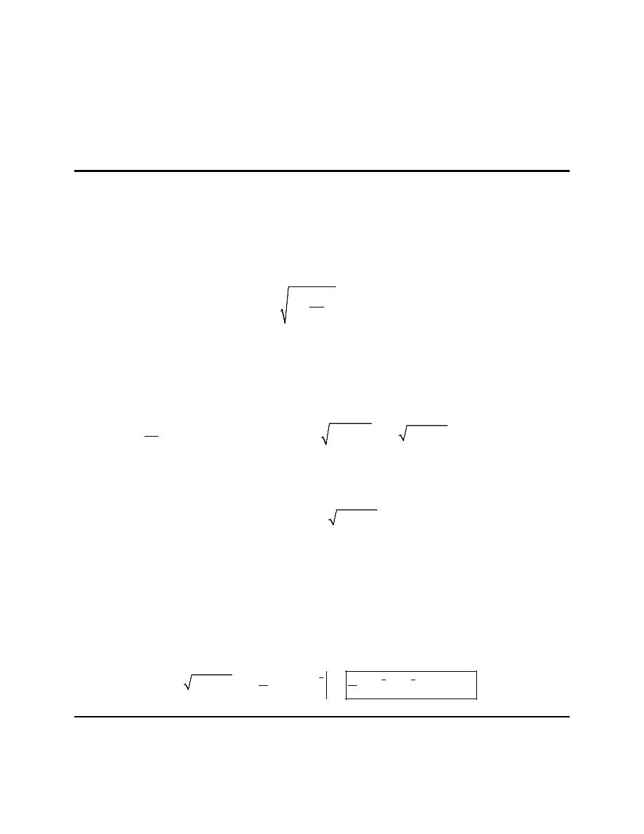
1. Find the center of mass for the region bounded by
2
4
y
x
= −
that is in the first quadrant.
Step 1
Let’s start out with a quick sketch of the region, with the center of mass indicated by the dot (the
coordinates of this dot are of course to be determined in the final step…..).
We’ll also need the area of this region so let’s find that first.
(
)
2
2
2
3
16
1
3
3
0
0
4
4
A
x dx
x
x
=
−
=
−
=
∫
Step 2
Next we need to compute the two moments. We didn’t include the density in the computations below
because it will only cancel out in the final step.
(
)
(
)
(
)
(
)
(
)
2
2
2
2
2
2
4
3
5
8
128
1
1
1
1
2
2
2
3
5
15
0
0
0
2
2
2
2
3
2
4
1
4
0
0
0
4
16 8
16
4
4
2
4
x
y
M
x
dx
x
x
dx
x
x
x
M
x
x
dx
x
x dx
x
x
=
−
=
−
+
=
−
+
=
=
−
=
−
=
−
=
∫
∫
∫
∫
Step 3
Finally the coordinates of the center of mass is,
Calculus II
© 2007 Paul Dawkins
17
http://tutorial.math.lamar.edu/terms.aspx
( )
( )
( )
( )
128
15
16
16
3
3
4
3
8
4
5
y
x
M
M
x
y
M
M
ρ
ρ
ρ
ρ
=
=
=
=
=
=
The center of mass is then :
( )
3
8
4
5
,
.
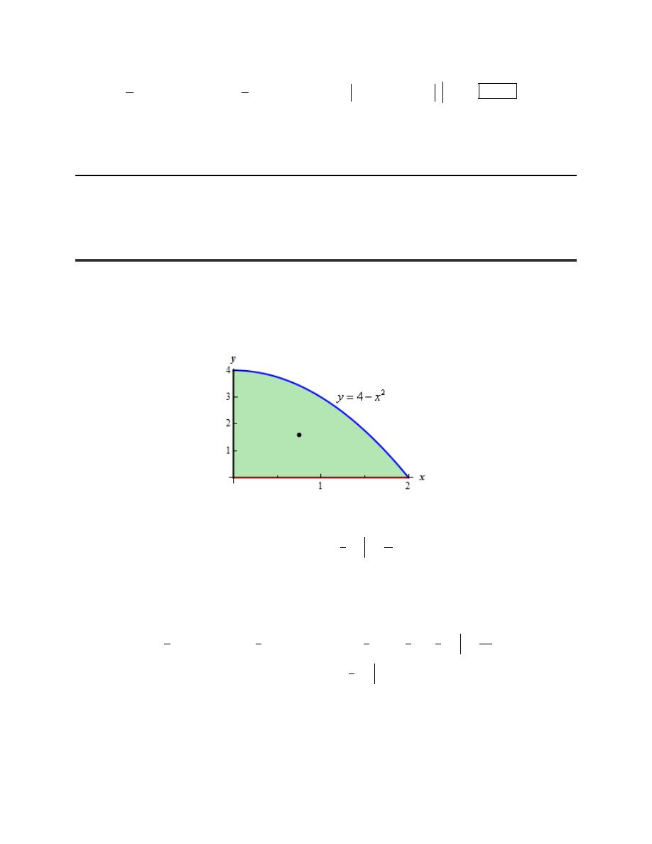
2. Find the center of mass for the region bounded by
3
x
y
−
= − e
, the x-axis,
2
x
=
and the y-axis.
Step 1
Let’s start out with a quick sketch of the region, with the center of mass indicated by the dot (the
coordinates of this dot are of course to be determined in the final step…..).
We’ll also need the area of this region so let’s find that first.
(
)
2
2
0
0
2
3
3
5
x
x
A
dx
x
−
−
−
=
−
=
+
= +
∫
e
e
e
Step 2
Next we need to compute the two moments. We didn’t include the density in the computations below
because it will only cancel out in the final step.
(
)
(
)
(
)
(
)
(
)
2
2
2
2
25
1
1
1
1
1
2
2
2
2
4
4
0
0
0
2
2
2
2
3
2
0
0
0
2
2
2
4
2
3
9 6
9
6
3
3
3
5 3
x
y
x
x
x
x
x
x
x
x
x
M
dx
dx
x
M
x
dx
x
x
dx
x
x
−
−
−
−
−
−
−
−
−
−
−
−
=
−
=
−
+
=
+
−
= +
−
=
−
=
−
=
+
+
= +
∫
∫
∫
∫
e
e
e
e
e
e
e
e
e
e
e
e
For the second term in the
y
M
integration we used the following integration by parts.
(
)
x
x
x
x
x
x
x
x
x
x
x
dx
u
x
du
dx
dv
dx v
x
dx
x
dx
x
x
−
−
−
−
−
−
−
−
−
−
=
=
=
= −
= −
+
= −
−
= −
+
∫
∫
∫
e
e
e
e
e
e
e
e
e
e
The minus sign here canceled with the minus sign that was in front of the term in the full integral.
Calculus II
© 2007 Paul Dawkins
18
http://tutorial.math.lamar.edu/terms.aspx
Make sure you don’t forget integration by parts! It is a fairly common integration technique for these
kinds of problems.
Step 3
Finally the coordinates of the center of mass is,
(
)
(
)
(
)
(
)
25
1
4
4
2
2
4
2
2
5 3
3
1.05271
1.29523
5
5
y
x
M
M
x
y
M
M
ρ
ρ
ρ
ρ
−
−
−
−
−
+
+
−
=
=
=
=
=
=
+
+
e
e
e
e
e
The center of mass is then :
(
)
1.05271, 1.29523
.
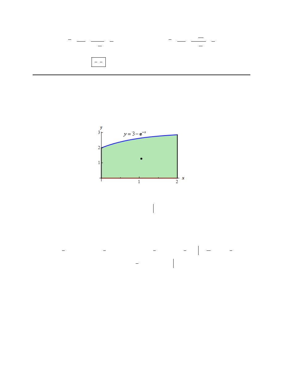
3. Find the center of mass for the triangle with vertices (0, 0), (-4, 2) and (0,6).
Step 1
Let’s start out with a quick sketch of the region, with the center of mass indicated by the dot (the
coordinates of this dot are of course to be determined in the final step…..).
We’ll leave it to you verify the equations of the upper and lower leg of the triangle.
We’ll also need the area of this region so let’s find that first.
(
)
(
)
(
)
0
0
0
2
3
3
1
2
2
4
4
4
4
6
6
6
12
A
x
x dx
x
dx
x
x
−
−
−
=
+ − −
=
+
=
+
=
∫
∫
Step 2
Next we need to compute the two moments. We didn’t include the density in the computations below
because it will only cancel out in the final step.
(
)
(
)
(
)
(
)
(
)
(
)
(
)
0
0
0
2
2
2
3
2
3
1
1
1
2
2
8
8
4
4
4
0
0
0
2
3
2
3
1
1
2
2
2
4
4
4
6
6
18
3
18
32
6
6
3
16
x
y
M
x
x
dx
x
x
dx
x
x
x
M
x
x
x
dx
x
x dx
x
x
−
−
−
−
−
−
=
+
− −
=
+
+
=
+
+
=
=
+ − −
=
+
=
+
= −
∫
∫
∫
∫
Step 3
Calculus II
© 2007 Paul Dawkins
19
http://tutorial.math.lamar.edu/terms.aspx
Finally the coordinates of the center of mass is,
(
)
( )
( )
( )
16
32
4
8
12
3
12
3
y
x
M
M
x
y
M
M
ρ
ρ
ρ
ρ
−
=
=
= −
=
=
=
The center of mass is then :
(
)
8
4
3
3
,
−
.
Hydrostatic Pressure and Force
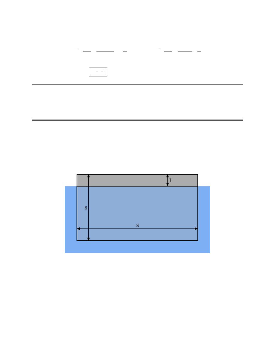
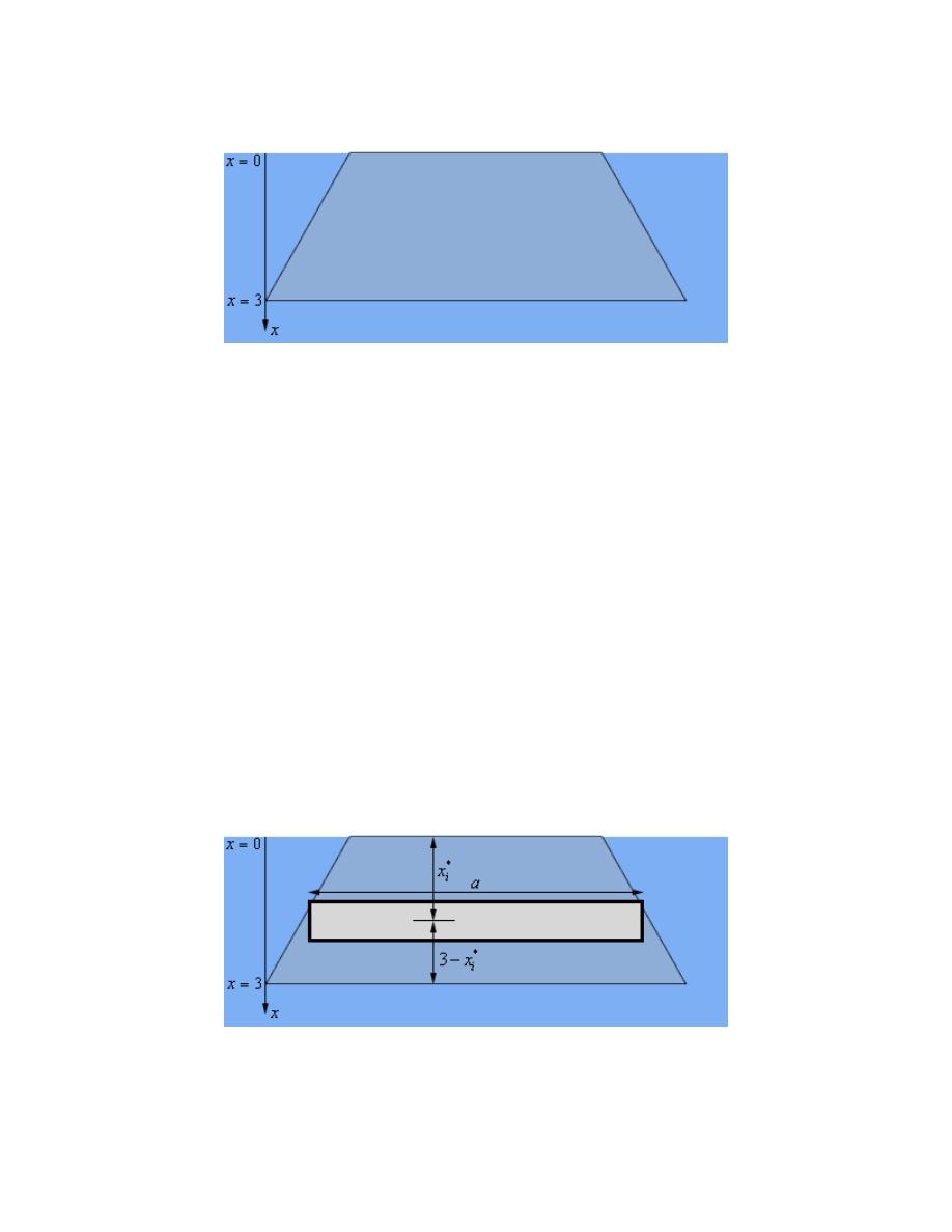
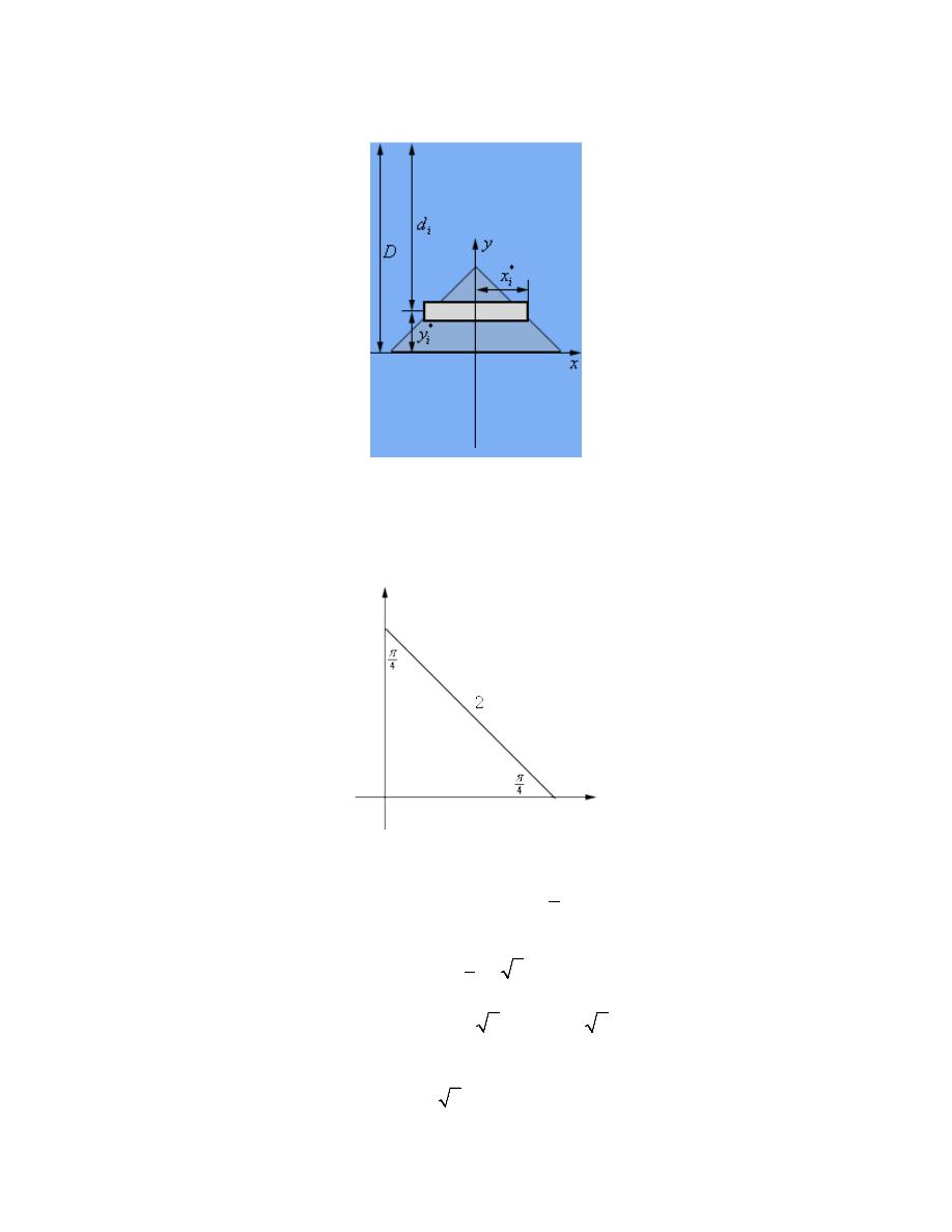
1. Find the hydrostatic force on the plate submerged in water as shown in the image below.
Consider the top of the blue “box” to be the surface of the water in which the plate is submerged. Note as
well that the dimensions in the image will not be perfectly to scale in order to better fit the plate in the
image. The lengths given in the image are in meters.
Hint : Start off by defining an “axis system” for the figure.
Step 1
The first thing we should do is define an axis system for the portion of the plate that is below the water.
Calculus II
© 2007 Paul Dawkins
20
http://tutorial.math.lamar.edu/terms.aspx
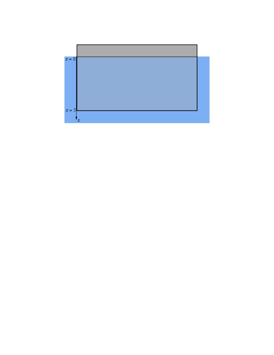
Note that we started the x-axis at the surface of the water and by doing this x will give the depth of any
point on the plate below the surface of the water. This in turn means that the bottom of the plate will be
defined by
5
x
=
.
It is always useful to define some kind of axis system for the plate to help with the rest of the problem.
There are lots of ways to actually define the axis system and how we define them will in turn affect how
we work the rest of the problem. There is nothing special about one definition over another but there is
often an “easier” axis definition and by “easier’ we mean is liable to make some portions of the rest of the
work go a little easier.
Hint : At this point it would probably be useful to break up the plate into horizontal strips and get a sketch
of a representative strip.
Step 2
As we did in the notes we’ll break up the portion of the plate that is below the surface of the water into n
horizontal strips of width
x
∆
and we’ll let each strip be defined by the interval
[
]
1
,
i
i
x
x
−
with
1, 2, 3,
i
n
=
. Finally we’ll let
*
i
x
be any point that is in the interval and hence will be some point on
the strip.
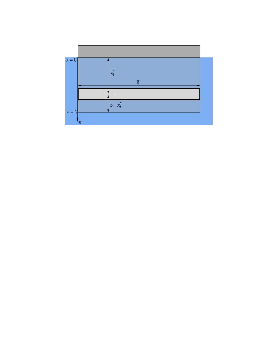
Below is yet another sketch of the plate only this time we’ve got a representative strip sketched on the
plate. Note that the strip is “thicker” than the strip really should be but it will make it easier to see what
the strip looks like and get all of the appropriate lengths clearly listed.
Calculus II
© 2007 Paul Dawkins
21
http://tutorial.math.lamar.edu/terms.aspx
Now
*
i
x
is a point from the interval defining the strip and so, for sufficiently thin strips, it is safe to
assume that the strip will be at the point
*
i
x
below the surface of the water as shown in the figure above.
In other words, the strip is a distance of
*
i
x
below the surface of the water.
Also, because our plate is a rectangle we know that each strip will have a width of 8.
Hint : What is the hydrostatic pressure and force on the representative strip?
Step 3
We’ll assume that the strip is sufficiently thin so the hydrostatic pressure on the strip will be constant and
is given by,
(
)(
)
*
*
1000 9.81
9810
i
i
i
i
P
gd
x
x
ρ
=
=
=
This, in turn, means that the hydrostatic force on each strip is given by,
(
)
( )( )
*
*
9810
8
78480
i
i
i
i
i
F
P A
x
x
x
x
=
=
∆
=
∆
Hint : How can we use the result from the previous step to approximate the total hydrostatic force on the
plate and how can we modify that to get an expression for the actual hydrostatic force on the plate?
Step 4
We can now approximate the total hydrostatic force on plate as the sum off the force on each of the strips.
Or,
*
1
78480
n
i
i
F
x
x
=
≈
∆
∑
Calculus II
© 2007 Paul Dawkins
22
http://tutorial.math.lamar.edu/terms.aspx
Now, we can get an expression for the actual hydrostatic force on the plate simply by letting n go to
infinity.
Or in other words, we take the limit as follows,
*
1
lim
78480
n
i
n
i
F
x
x
→∞
=
=
∆
∑
Hint : You do recall the definition of the definite integral don’t you?
Step 5
Finally, we know from the definition of the definite integral that this is nothing more than the following
definite integral that we can easily compute.
5
5
2
0
0
78480
39240
981, 000
F
x dx
x
N
=
=
=
∫
2. Find the hydrostatic force on the plate submerged in water as shown in the image below.
Consider the top of the blue “box” to be the surface of the water in which the plate is submerged. Note as
well that the dimensions in the image will not be perfectly to scale in order to better fit the plate in the
image. The lengths given in the image are in meters.
Hint : Start off by defining an “axis system” for the figure.
Step 1
The first thing we should do is define an axis system for the portion of the plate that is below the water.
Calculus II
© 2007 Paul Dawkins
23
http://tutorial.math.lamar.edu/terms.aspx
Note that we started the x-axis at the surface of the water and by doing this x will give the depth of any
point on the plate below the surface of the water. This in turn means that the bottom of the plate will be
defined by
3
x
=
.
It is always useful to define some kind of axis system for the plate to help with the rest of the problem.
There are lots of ways to actually define the axis system and how we define them will in turn affect how
we work the rest of the problem. There is nothing special about one definition over another but there is
often an “easier” axis definition and by “easier’ we mean is liable to make some portions of the rest of the
work go a little easier.
Hint : At this point it would probably be useful to break up the plate into horizontal strips and get a sketch
of a representative strip.
Step 2
As we did in the notes we’ll break up the plate into n horizontal strips of width
x
∆
and we’ll let each
strip be defined by the interval
[
]
1
,
i
i
x
x
−
with
1, 2, 3,
i
n
=
. Finally we’ll let
*
i
x
be any point that is in
the interval and hence will be some point on the strip.
Below is yet another sketch of the plate only this time we’ve got a representative strip sketched on the
plate. Note that the strip is “thicker” than the strip really should be but it will make it easier to see what
the strip looks like and get all of the appropriate lengths clearly listed.
Calculus II
© 2007 Paul Dawkins
24
http://tutorial.math.lamar.edu/terms.aspx
Now
*
i
x
is a point from the interval defining the strip and so, for sufficiently thin strips, it is safe to
assume that the strip will be at the point
*
i
x
below the surface of the water as shown in the figure above.
In other words, the strip is a distance of
*
i
x
below the surface of the water.
The width of each of the strips will be dependent on the depth of the strip and so temporarily let’s just call
the width a.
To determine the value of a for each strip let’s consider the following set of similar triangles.
This is the triangle of “empty” space to the left of the plate. The overall height of the larger triangle is the
same as the plate, namely 3. The overall width of the larger triangle is 1.5. We arrived at this number by
noticing that the top of the plate was 3 meters shorter than the bottom and if we assume the top was
perfectly centered over the bottom there must be 1.5 meters of “empty” space to either side of the top.
The top of the smaller triangle corresponds to the strip on the plate. We’ll call the width of the smaller
triangle b. and the height of the smaller triangle must be
*
3
i
x
−
for each strip.
Because the two triangles are similar triangles we have the following equation.
(
)
*
*
1.5
1
3
3
3
2
i
i
b
b
x
x
=
=
−
−

Calculus II
© 2007 Paul Dawkins
25
http://tutorial.math.lamar.edu/terms.aspx
Note that while we looked only at the empty space to the left of the plate we’d get an almost identical
triangle for the empty space to the right of the plate. The only exception would be that it would be a
mirror image of this triangle.
Now, let’s get back to the width of the strip in our picture of the plate. Assuming that the top is centered
over the bottom of the plate we can see that we have to have,
( )
(
)
*
*
1
2
7
2
3 2
3
4
i
i
a
b
x
x
= −
= −
−
= +
Hint : What is the hydrostatic pressure and force on the representative strip?
Step 3
We’ll assume that the strip is sufficiently thin so the hydrostatic pressure on the strip will be constant and
is given by,
(
)(
)
*
*
1000 9.81
9810
i
i
i
i
P
gd
x
x
ρ
=
=
=
This, in turn, means that the hydrostatic force on each strip is given by,
(
) (
)
( )
( )
2
*
*
*
*
9810
4
19620 4
i
i
i
i
i
i
i
F
P A
x
x
x
x
x
x
=
=
+
∆
=
+
∆
Hint : How can we use the result from the previous step to approximate the total hydrostatic force on the
plate and how can we modify that to get an expression for the actual hydrostatic force on the plate?
Step 4
We can now approximate the total hydrostatic force on plate as the sum off the force on each of the strips.
Or,
( )
2
*
*
1
19620 4
n
i
i
i
F
x
x
x
=
≈
+
∆
∑
Now, we can get an expression for the actual hydrostatic force on the plate simply by letting n go to
infinity.
Or in other words, we take the limit as follows,
( )
2
*
*
1
lim
19620 4
n
i
i
n
i
F
x
x
x
→∞
=
=
+
∆
∑
Hint : You do recall the definition of the definite integral don’t you?
Step 5
Finally, we know from the definition of the definite integral that this is nothing more than the following
definite integral that we can easily compute.
(
)
(
)
3
3
2
2
3
1
3
0
0
19620 4
19620 2
529, 740
F
x
x
dx
x
x
N
=
+
=
+
=
∫
Calculus II
© 2007 Paul Dawkins
26
http://tutorial.math.lamar.edu/terms.aspx
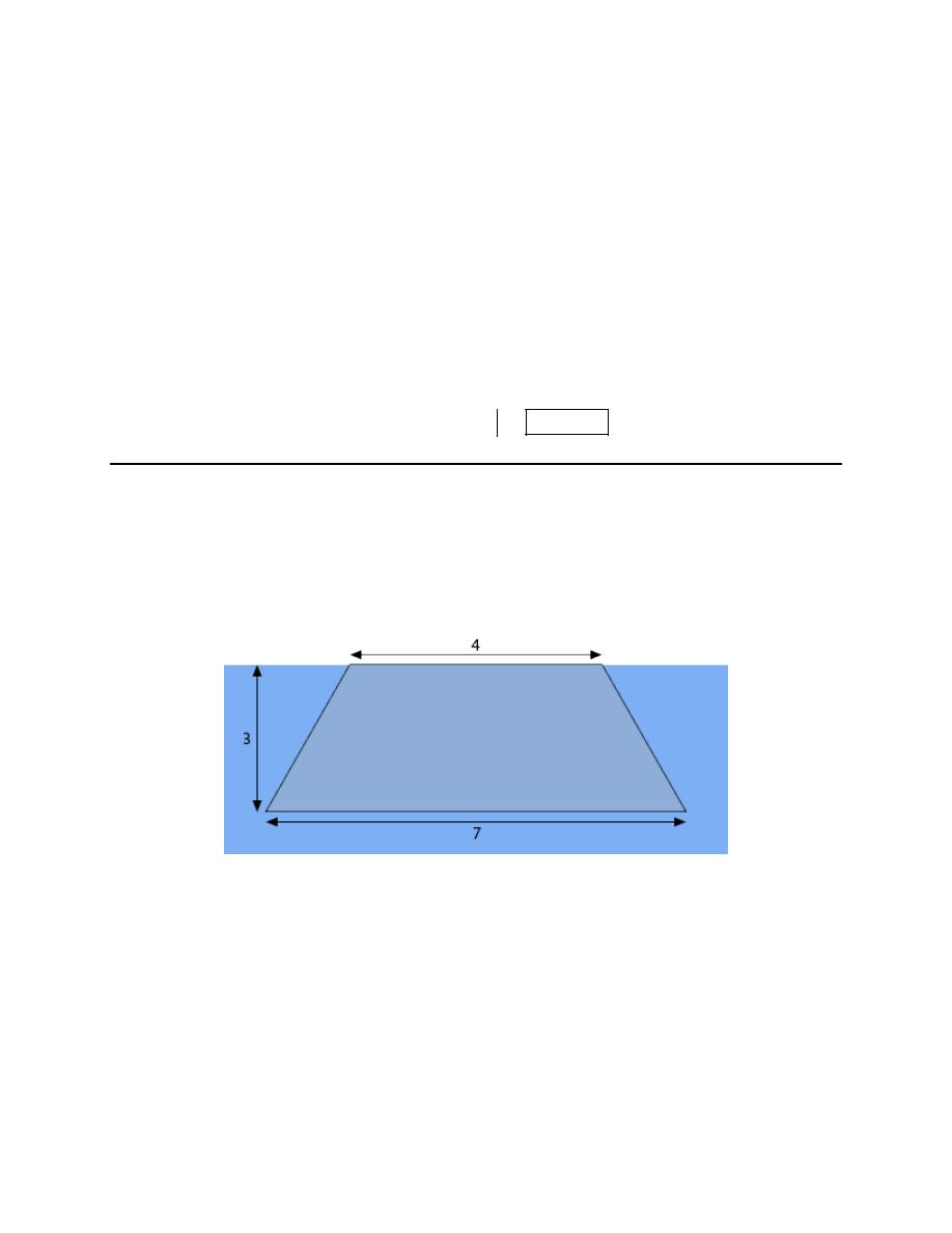
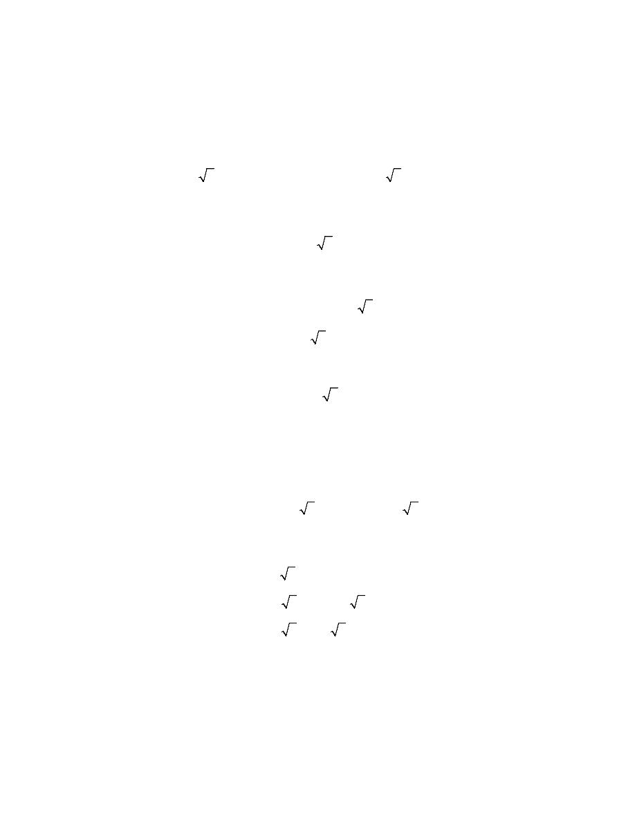
3. Find the hydrostatic force on the plate submerged in water as shown in the image below. The plate in
this case is the top half of a diamond formed from a square whose sides have a length of 2.
Consider the top of the blue “box” to be the surface of the water in which the plate is submerged. Note as
well that the dimensions in the image will not be perfectly to scale in order to better fit the plate in the
image. The lengths given in the image are in meters.
Hint : Start off by defining an “axis system” for the figure.
Step 1
The first thing we should do is define an axis system for the portion of the plate that is below the water.
Calculus II
© 2007 Paul Dawkins
27
http://tutorial.math.lamar.edu/terms.aspx
In this case since we had the top half a diamond formed from a square it seemed convenient to center the
axis system in the middle of the diamond.
It is always useful to define some kind of axis system for the plate to help with the rest of the problem.
There are lots of ways to actually define the axis system and how we define them will in turn affect how
we work the rest of the problem. There is nothing special about one definition over another but there is
often an “easier” axis definition and by “easier’ we mean is liable to make some portions of the rest of the
work go a little easier.
Hint : At this point it would probably be useful to break up the plate into horizontal strips and get a sketch
of a representative strip.
Step 2
As we did in the notes we’ll break up the plate into n horizontal strips of width
y
∆
and we’ll let each
strip be defined by the interval
[
]
1
,
i
i
y
y
−
with
1, 2, 3,
i
n
=
. Finally we’ll let
*
i
y
be any point that is in
the interval and hence will be some point on the strip.
Below is yet another sketch of the plate only this time we’ve got a representative strip sketched on the
plate. Note that the strip is “thicker” than the strip really should be but it will make it easier to see what
the strip looks like and get all of the appropriate lengths clearly listed.
Calculus II
© 2007 Paul Dawkins
28
http://tutorial.math.lamar.edu/terms.aspx
We’ve got a few quantities to determine at this point. To do that it would be convenient to have an
equation for one of the sides of the plate. Let’s take a look at the side in the first quadrant. Here is a
quick sketch of that portion of the plate.
Now, as noted above we have the top half of a diamond formed from a square and so we can see that the
“triangle” formed in the first quadrant by the plate must be an isosceles right triangle whose hypotenuse is
2 and the two interior angles other than the right angle must be
4
π
. Therefore the bottom/left side of the
triangle must be,
( )
4
side
2 tan
2
π
=
=
This means we know that the x and y-intercepts are
(
)
2, 0
and
(
)
0, 2
respectively and so the
equation for the line representing the hypotenuse must be,
2
y
x
=
−
Calculus II
© 2007 Paul Dawkins
29
http://tutorial.math.lamar.edu/terms.aspx
Okay, let’s get the various quantities in the figure.
We’ll start with
*
i
x
. This we can get directly from the equation above by acknowledging that if we are at
*
i
x
then the y value must be
*
i
y
. In other words, plugging these into the equation and solving gives,
*
*
*
*
2
2
i
i
i
i
y
x
x
y
=
−
→
=
−
Notice as well that the width of each strip in terms of
*
i
y
is then,
(
)
*
*
2
2
2
i
i
x
y
=
−
Next, let’s get D. First we can see that D is the distance from the surface of the water to the x-axis in our
figure. We know that the distance from the surface of the water to the top of the plate is 4 meters. Also,
we found above that the top point of the plate is a distance of
2
above the x-axis. So, we then have,
4
2
D
= +
Finally, the depth of each strip below the surface of the water is,
*
*
4
2
i
i
i
d
D
y
y
= −
= +
−
Hint : What is the hydrostatic pressure and force on the representative strip?
Step 3
We’ll assume that the strip is sufficiently thin so the hydrostatic pressure on the strip will be constant and
is given by,
(
)(
)
(
)
(
)
*
*
1000 9.81 4
2
9810 4
2
i
i
i
i
P
gd
y
y
ρ
=
=
+
−
=
+
−
This, in turn, means that the hydrostatic force on each strip is given by,
(
)
( )
( )
(
) (
)
( )
(
)(
)
( )
*
*
*
*
*
*
9810 4
2
2
9810 4
2
2
2
19620 4
2
2
i
i
i
i
i
i
i
i
i
F
P A
y
x
y
y
y
y
y
y
y
=
=
+
−
∆
=
+
−
−
∆
=
+
−
−
∆
Hint : How can we use the result from the previous step to approximate the total hydrostatic force on the
plate and how can we modify that to get an expression for the actual hydrostatic force on the plate?
Step 4
We can now approximate the total hydrostatic force on plate as the sum off the force on each of the strips.
Or,
Calculus II
© 2007 Paul Dawkins
30
http://tutorial.math.lamar.edu/terms.aspx
(
)(
)
( )
*
*
1
19620 4
2
2
n
i
i
i
F
y
y
y
=
≈
+
−
−
∆
∑
Now, we can get an expression for the actual hydrostatic force on the plate simply by letting n go to
infinity.
Or in other words, we take the limit as follows,
(
)(
)
( )
*
*
1
lim
19620 4
2
2
n
i
i
n
i
F
y
y
y
→∞
=
=
+
−
−
∆
∑
Hint : You do recall the definition of the definite integral don’t you?
Step 5
Finally, we know from the definition of the definite integral that this is nothing more than the following
definite integral that we can easily compute.
(
)(
)
(
)
(
)
(
) (
)
(
)
2
0
2
2
0
2
3
2
1
3
0
19620 4
2
2
19620
4 2 2
2 4 2
19620
2
2
2 4 2
96, 977.9
F
y
y dy
y
y
dy
y
y
y
N
=
+
−
−
=
− +
+ +
=
− +
+ +
=
∫
∫
Probability
1. Let,
( )
(
)
2
3
20
if 2
18
37760
0
otherwise
x
x
x
f x
−
≤ ≤
=
(a) Show that
( )
f x
is a probability density function.
(b) Find
(
)
7
P X
≤
.
(c) Find
(
)
7
P X
≥
.
(d) Find
(
)
3
14
P
X
≤
≤
.
(e) Determine the mean value of X.

Calculus II
© 2007 Paul Dawkins
31
http://tutorial.math.lamar.edu/terms.aspx
(a) Show that
( )
f x
is a probability density function.
Okay, to show that this function is a probability density function we can first notice that in the range
2
18
x
≤ ≤
the function is positive and will be zero everywhere else and so the first condition is satisfied.
The main thing that we need to do here is show that
( )
1
f x dx
∞
−∞
=
∫
.
( )
(
)
(
)
18
2
3
37760
2
18
18
2
3
3
4
3
3
20
1
37760
37760
3
4
2
2
20
20
1
f x dx
x
x dx
x
x dx
x
x
∞
−∞
=
−
=
−
=
−
=
∫
∫
∫
The integral is one and so this is in fact a probability density function.
(b) Find
(
)
7
P X
≤
.
First note that because of our limits on x for which the function is not zero this is equivalent to
(
)
2
7
P
X
≤
≤
. Here is the work for this problem.
(
)
(
)
(
)
(
)
7
7
2
3
4
3
3
20
1
37760
37760
3
4
2
2
7
2
7
20
0.130065
P X
P
X
x
x dx
x
x
≤
=
≤
≤
=
−
=
−
=
∫
Note that we made use of the fact that we’ve already done the indefinite integral itself in the first part. All
we needed to do was change limits from that part to match the limits for this part.
(c) Find
(
)
7
P X
≥
.
First note that because of our limits on x for which the function is not zero this is equivalent to
(
)
7
18
P
X
≤
≤
. Here is the work for this problem.
(
)
(
)
(
)
(
)
18
18
2
3
4
3
3
20
1
37760
37760
3
4
7
7
7
7
18
20
0.869935
P X
P
X
x
x dx
x
x
≥
=
≤
≤
=
−
=
−
=
∫
Note that we made use of the fact that we’ve already done the indefinite integral itself in the first part. All
we needed to do was change limits from that part to match the limits for this part.
(d) Find
(
)
7
P X
≥
.
Not much to do here other than compute the integral.
(
)
(
)
(
)
14
14
2
3
4
3
3
20
1
37760
37760
3
4
3
3
3
14
20
0.677668
P
X
x
x dx
x
x
≤
≤
=
−
=
−
=
∫
Note that we made use of the fact that we’ve already done the indefinite integral itself in the first part. All
we needed to do was change limits from that part to match the limits for this part.
(e) Determine the mean value of X.
For this part all we need to do is compute the following integral.

Calculus II
© 2007 Paul Dawkins
32
http://tutorial.math.lamar.edu/terms.aspx
( )
(
)
(
)
18
2
3
37760
2
18
18
3
4
4
5
3
3
1
37760
37760
5
2
2
20
20
5
11.6705
x f x dx
x
x
x
dx
x
x dx
x
x
µ
∞
−∞
=
=
−
=
−
=
−
=
∫
∫
∫
The mean value of X is then 11.6705.
2. For a brand of light bulb the probability density function of the life span of the light bulb is given by
the function below, where t is in months.
( )
25
0.04
if 0
0
if 0
t
t
f t
t
−
≥
=
<
e
(a) Verify that
( )
f t
is a probability density function.
(b) What is the probability that a light bulb will have a life span less than 8 months?
(c) What is the probability that a light bulb will have a life span more than 20 months?
(d) What is the probability that a light bulb will have a life span between 14 and 30 months?
(e) Determine the mean value of the life span of the light bulbs.
(a) Show that
( )
f t
is a probability density function.
Okay, to show that this function is a probability density function we can first notice that the exponential
portion is always positive regardless of the value of t we plug in and the remainder of the function is
always zero and so the first condition is satisfied.
The main thing that we need to do here is show that
( )
1
f x dx
∞
−∞
=
∫
.
( )
25
25
0
0
25
25
0
0.04
lim
0.04
lim
lim
1
0 1 1
n
n
n
n
n
t
t
t
n
f x dx
dt
dt
−
−
∞
∞
−∞
→∞
−
−
→∞
→∞
=
=
=
−
=
−
+ = + =
∫
∫
∫
e
e
e
e
The integral is one and so this is in fact a probability density function.
For this integral do not forget to properly deal with the infinite limit! If you don’t recall how to deal with
these kinds of integrals go back to the
Improper Integral section
and do a quick review!
(b) What is the probability that a light bulb will have a life span less than 8 months?

Calculus II
© 2007 Paul Dawkins
33
http://tutorial.math.lamar.edu/terms.aspx
What this problem is really asking us to compute is
(
)
8
P X
≤
. Also, because of our limits on t for
which the function is not zero this is equivalent to
(
)
0
8
P
X
≤
≤
. Here is the work for this problem.
(
)
(
)
8
8
25
25
0
0
8
0
8
0.04
0.273851
t
t
P X
P
X
dt
−
−
≤
=
≤
≤
=
= −
=
∫
e
e
(c) What is the probability that a light bulb will have a life span more than 20 months?
What this problem is really asking us to compute is
(
)
20
P X
≥
. Here is the work for this problem.
(
)
25
25
20
20
20
25
25
25
20
20
0.04
lim
0.04
lim
lim
0.449329
n
n
n
n
n
t
t
t
n
P X
dt
dt
−
−
∞
→∞
−
−
−
→∞
→∞
≥
=
=
=
−
=
−
+
=
∫
∫
e
e
e
e
e
For this integral do not forget to properly deal with the infinite limit! If you don’t recall how to deal with
these kinds of integrals go back to the
Improper Integral section
and do a quick review!
(d) What is the probability that a light bulb will have a life span between 14 and 30 months?
What this problem is really asking us to compute is
(
)
14
30
P
X
≤
≤
. Here is the work for this problem.
(
)
30
30
25
25
14
14
14
30
0.04
0.270015
t
t
P
X
dt
−
−
≤
≤
=
= −
=
∫
e
e
(e) Determine the mean value of the life span of the light bulbs.
For this part all we need to do is compute the following integral.
( )
(
)
( )
25
25
0
0
25
25
25
25
0
25
1
25
25
25
0.04
lim
0.04
lim
25
lim
25
25
1
lim
25
25
lim
25 0
25
25
n
n
n
n
n
n
n
t
t
t
t
n
n
n
n
n
t f t dt
t
dt
t
dt
t
n
n
µ
−
−
∞
∞
−∞
→∞
−
−
−
−
→∞
→∞
−
→∞
→∞
=
=
=
=
−
−
=
−
−
− −
=
−
−
+
=
−
−
+
=
∫
∫
∫
e
e
e
e
e
e
e
e
e
The mean value of the life span of the light bulbs is then 25 months.
We had to use integration by parts to do the integral. Here is that work if you need to see it.

Calculus II
© 2007 Paul Dawkins
34
http://tutorial.math.lamar.edu/terms.aspx
25
25
25
25
25
25
25
25
0.04
0.04
0.04
25
0.04
25
t
t
t
t
t
t
t
t
t
dt
u
t
du
dt
dv
dt
v
t
dt
t
dt
t
−
−
−
−
−
−
−
−
=
=
=
= −
= −
+
= −
−
∫
∫
∫
e
e
e
e
e
e
e
e
Also, for the limit of the first term we used L’Hospital’s Rule to do the limit.
3. Determine the value of c for which the function below will be a probability density function.
( )
(
)
3
4
8
if 0
8
0
otherwise
c
x
x
x
f x
−
≤ ≤
=
Solution
This problem is actually easier than it might look like at first glance.
First, in order for the function to be a probability density function we know that the function must be
positive or zero for all x. We can see that for
0
8
x
≤ ≤
we have
3
4
8
0
x
x
−
≥
. Therefore, we need to
require that whatever c is it must be a positive number.
To find c we’ll use the fact that we must also have
( )
1
f x dx
∞
−∞
=
∫
. So, let’s compute this integral (with
the c in the function) and see what we get.
( )
(
)
(
)
8
8
3
4
4
5
8192
1
5
5
0
0
8
2
f x dx
c
x
x
dx
c
x
x
c
∞
−∞
=
−
=
−
=
∫
∫
So, we can see that in order for this integral to have a value of 1 (as it must in order for the function to be
a probability density function) we must have,
5
8192
c
=
and note that this is also a positive number as we determined earlier was required.