
.
Ahmad_engineer21@yahoo.com
M
A
T
L
A
B
:
-
.
:
-
.
:
-
.
:
-
)
,
,
(
:
-
)
,
,
,
,
(
:
-
Ahmad_Engineer21@yahoo.com
:
-
.
.
.
:
-
2010
2011
.
:
-
.
:
-
.

.
Ahmad_engineer21@yahoo.com
,
,
...
.
.
.
. .
.
.
......................
............................
..............................
.........................
........................
...................
.................
.....................
........................
................

.
Ahmad_engineer21@yahoo.com
1
-
%---------------------------------
clc
clear
a=4;
b=5;
c=7;
d=a+b+c
%---------------------------------
clc
clear
a=[2 3 4 6 7 8 9 10];
sum(a)
%----------------------------------
2
-
%---------------------------------
clc
clear
a=4;
b=5;
c=7;
d=a-b-c
%---------------------------------
3
-
%---------------------------------
clc
clear
a=4;
b=5;
c=7;
d=a*b*c
%---------------------------------
clc
clear
a=4;
b=5;
c=7;
d=conv(a,b)
%or d=conv(a,conv(b,c))
f=conv(d,c)
%----------------------------------
s=[4 5 7];
prod(s)
%-------------------------
4
-
%---------------------------------
clc
clear
a=4;
b=5;
c=7;
d=a/b
f=d/c
%---------------------------------

.
Ahmad_engineer21@yahoo.com
clc
clear
a=4;
b=5;
c=7;
d=deconv(a,b)
%or d=deconv(deconv(a,b),c)
f=deconv(d,c)
%----------------------------------
5
-
((5*log10(x)+2*x^2*sin(x)+sqrt(x)*lin(x))
f=-----------------------------------------
(exp(6*x^3)+3*x^4+sin(lin(x)))
%---------------------------------
clc
clear
x=1;
f=deconv((5*log10(x)+2*x^2*sin(x)+sqrt(x)*log(x)),(exp(6*x^3)+3*x^4+s
in(log(x))))
%---------------------------------
clc
clear
x=1;
f=(5*log10(x)+2*x^2*sin(x)+sqrt(x)*log(x))/(exp(6*x^3)+3*x^4+sin(log
(x)))
%----------------------------------
6
-
%---------------------------------
clc
clear
syms
x
f=((x^5)+(5*x^4)+(4*x^3)-(2*x^2)-(8*x)+9)
d=diff(f,x)
%---------------------------
clc
clear
syms
x
f=((x^5)+(5*x^4)+(4*x^3)-(2*x^2)-(8*x)+9)
d=diff(f,2)
%------------------------------
%---------------------------------
clc
clear
syms
x
f=(1/(1+x^2))
d=diff(f,x)
%---------------------------
7
-
%---------------------------------
clc
clear
syms
x
f=(1/(1+x^2))
.
Ahmad_engineer21@yahoo.com
d=int(f,x)
%---------------------------
clc
clear
syms
x
f=((x^5)+(5*x^4)+(4*x^3)-(2*x^2)-(8*x)+9)
d=int(f,x)
%------------------------------
%---------------------------
clc
clear
syms
x
f=((x^5)+(5*x^4)+(4*x^3)-(2*x^2)-(8*x)+9)
d=int(f,1,2)
%------------------------------
%---------------------------
clc
clear
syms
x
a
b
f=((x^5)+(5*x^4)+(4*x^3)-(2*x^2)-(8*x)+9)
d=int(f,a,b)
%------------------------------
8
-
.
Ahmad_engineer21@yahoo.com
%---------------------------------
clc
clear
syms
x
t
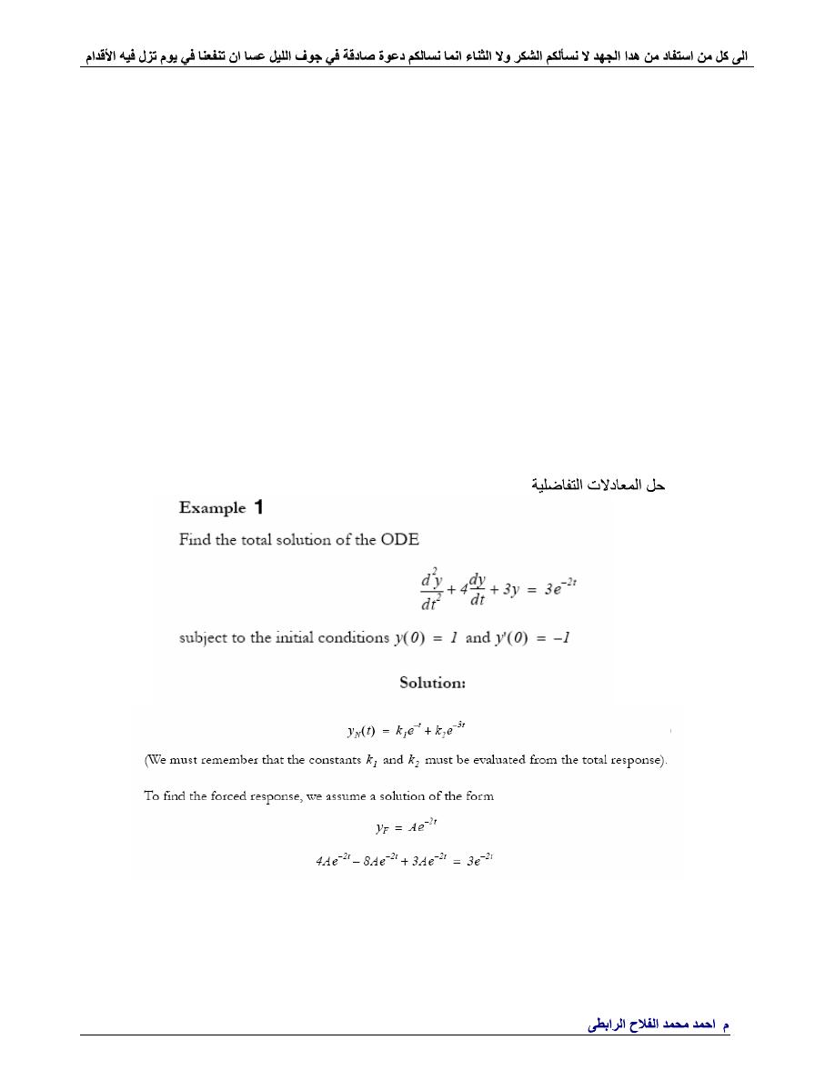
y=dsolve(
'D2y+4*Dy+3*y=3*exp(-2*t)'
,
'y(0)=1'
,
'Dy(0)=-1'
)
ezplot(y,[0 4])
%pretty(y)
%-----------------------------------
9
-
%-----------------------------------
clc
syms
k3
k4
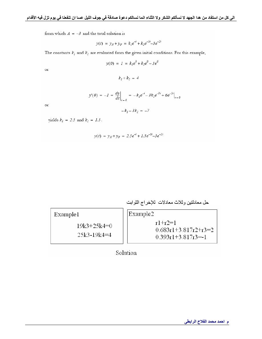
f1=19*k3+25*k4;
f2=25*k3-19*k4-4;
[k3 k4]=solve(f1,f2 )
%--------------------------------
clc
syms
r1
r2
r3
f1=r1+r2-1;
f2=0.683*r1+3.817*r2+r3-2;
.
Ahmad_engineer21@yahoo.com
f3=0.393*r1 + 3.817*r3+1
[r1 r2 r3]=solve(f1,f2,f3)
%------------------------------------------
Solution
%--------------------------------
clc
syms
x
y
z
alpha
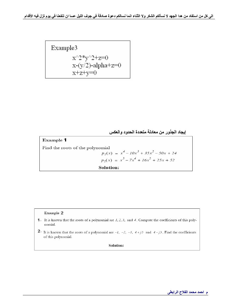
x^2*y^2+z=0
x-(y/2)-alpha+z=0
x+z+y=0
[x,y,z]=solve(
'x^2*y^2+z'
,
'x-(y/2)-alpha+z'
,
'x+z+y'
)
%----------------------------------
10
-
%-----------------------------------
clc
p1=[1 -10 35 -50 24];
f1=roots(p1)
%-----------------------------------
p2=[1 -7 0 16 25 52];
f2=roots(p2)
%----------------------------------
%--------------------------------
clc
r1=[1 2 3 4];
f1=poly(r1)
r2=[-1 -2 -3 -4+5j -4-5j ];
f2=poly(r2)
%----------------------------------
.
Ahmad_engineer21@yahoo.com
%--------------------------------
clc
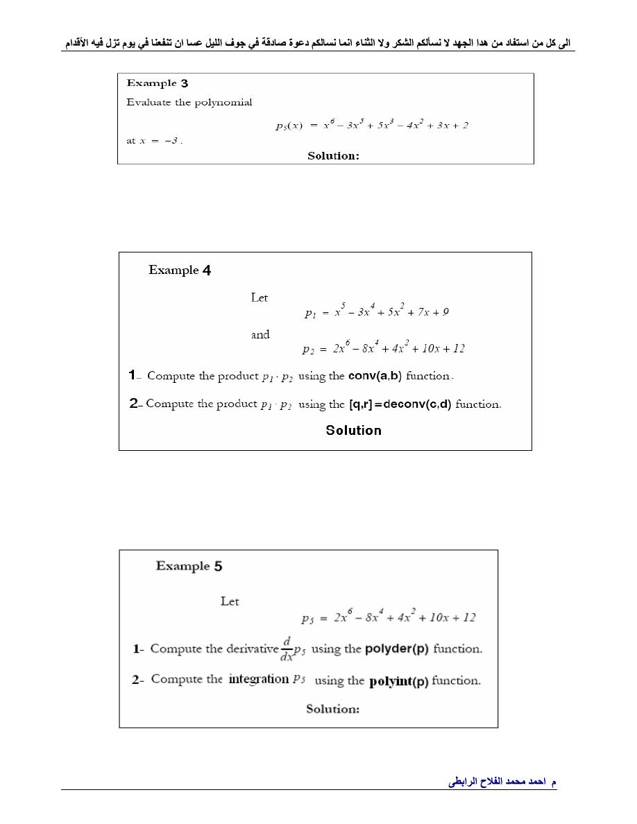
p1=[1 -3 0 5 -4 3 2];
f1=polyval(p1,-3)
%----------------------------------
%--------------------------------
clc
p1=[1 0 -3 0 5 7 9];
p2=[2 -8 0 0 4 10 12];
f1=conv(p1,p2)
[q,r]=deconv(p1,p2)
%----------------------------------
.
Ahmad_engineer21@yahoo.com
%--------------------------------
clc
clear
p5=[2 0 -8 0 4 10 12];
f1=polyder(p5)
f2=polyint(p5)
%----------------------------------
%--------------------------------
clc
clear
syms
x
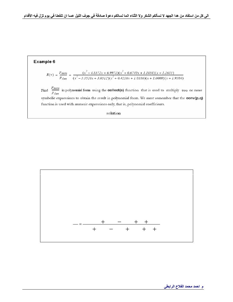
pnum=collect((x^2-4.8372*x+6.9971)*(x^2+0.6740*x+1.1058)*(x+1.1633))
pden=collect((x^23.3520*x+3.0512)*(x^2+0.4216*x+1.0186)*(x+1.0000)*(x
+1.9304))
R=pnum/pden
pretty(R)
%----------------------------------
Example 7
finds the residues, poles and direct term of a partial fraction expansion of the ratio of
two polynomials B(s)/A(s) .If there are no multiple roots,
B(s) R(1) R(2) R(n)
---- = -------- + -------- + ... + -------- + K(s)
A(s) s - P(1) s - P(2) s - P(n)
[R,P,K] = residue (B,A)
1
2
2
^
6
3
^
2
4
^
4
5
^
1
5
2
^
4
3
^
2
4
^
x
x
x
x
x
x
x
x
x
a
b
solution
%--------------------------------
clc
b=[1 2 -4 5 1];
a=[1 4 -2 6 2 1];
[R,P,K] = residue(b,a)
%----------------------------------
.
Ahmad_engineer21@yahoo.com
R = 0.2873 , -0.0973 + 0.1767i, -0.0973 - 0.1767i, 0.4536 + 0.0022i, 0.4536 - 0.0022i
P = -4.6832, 0.5276 + 1.0799i, 0.5276 - 1.0799i, -0.1860 + 0.3365i, -0.1860 - 0.3365i
K =0
11
-
%--------------------------------
clc
clear
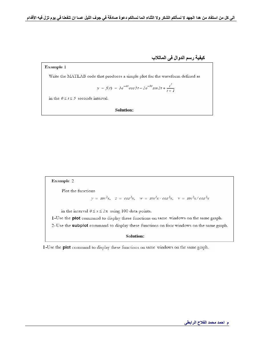
t=0: 0.01: 5
% Define t-axis in 0.01 increments
y=3.* exp(-4.* t).* cos(5 .* t)-2.* exp(-3.* t).* sin(2.* t) + t.^2./
(t+1)
plot(t,y);
grid;
xlabel(
't'
);
ylabel(
'y=f(t)'
);
title(
'Plot for Example A.13'
)
%----------------------------------
%--------------------------------
clc
clear
x=linspace(0,2*pi,100);
% Interval with 100 data points
y=(sin(x).^ 2);
z=(cos(x).^ 2);
w=y.* z;
v=y./ (z+eps);
% add eps to avoid division by zero
plot(x,y,
'b'
,x,z,
'g'
,x,w,
'r'
,x,v,
'y'
);
grid
on
axis([0 10 0 5]);
%-----------------------------------------------------------------
.
Ahmad_engineer21@yahoo.com
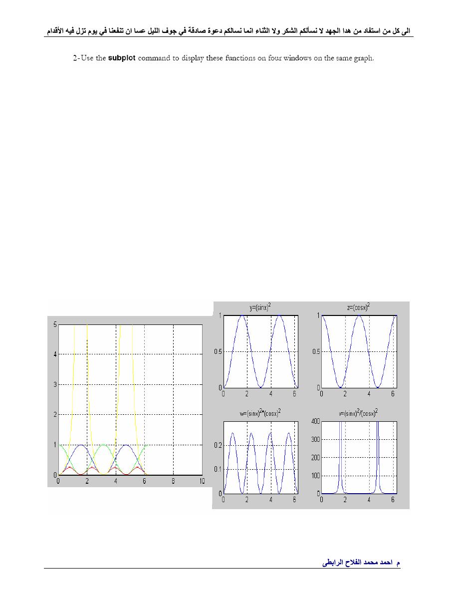
%-----------------------------------------------------------------
clc
clear
x=linspace(0,2*pi,100);
% Interval with 100 data points
y=(sin(x).^ 2);
z=(cos(x).^ 2);
w=y.* z;
v=y./ (z+eps);
subplot(221);
% upper left of four subplots
plot(x,y);
axis([0 2*pi 0 1]);
title(
'y=(sinx)^2'
);
grid
on
subplot(222);
% upper right of four subplots
plot(x,z);
axis([0 2*pi 0 1]);
title(
'z=(cosx)^2'
);
grid
on
subplot(223);
% lower left of four subplots
plot(x,w);
axis([0 2*pi 0 0.3]);
title(
'w=(sinx)^2*(cosx)^2'
);
grid
on
subplot(224);
% lower right of four subplots
plot(x,v);
axis([0 2*pi 0 400]);
title(
'v=(sinx)^2/(cosx)^2'
);
grid
on
%----------------------------------

.
Ahmad_engineer21@yahoo.com
:
-
for
clc
a=0;
disp(
'----------------------------------------------------'
)
for
i=1:10;
b=0;
for
j=1:10;
c(j) =a*b;
b=b+1;
end
c
disp(
'----------------------------------------------------'
)
a=a+1;
end
.
Ahmad_engineer21@yahoo.com
1
-
))
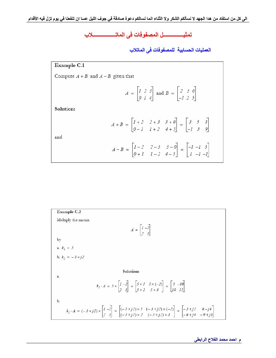
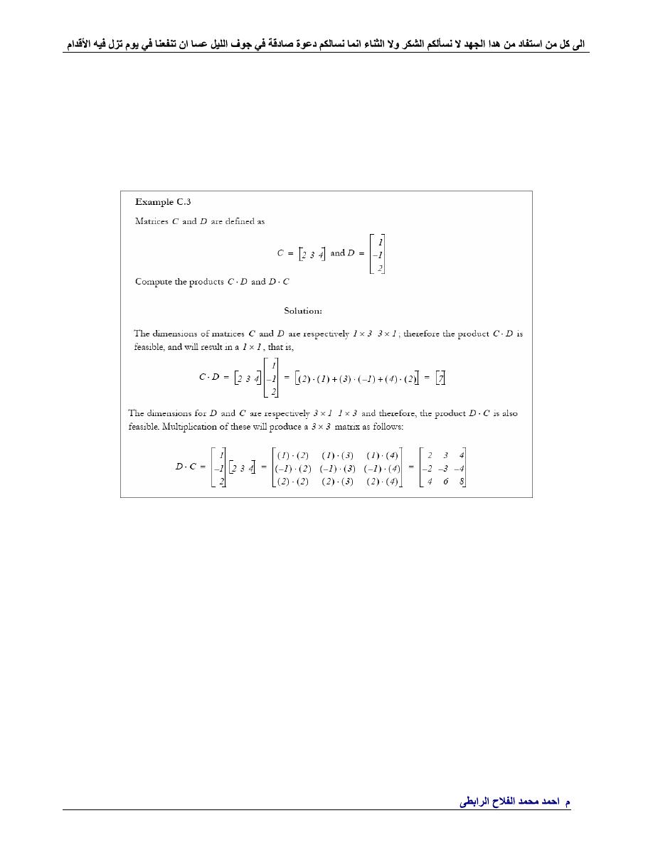
Matrix Operations
((
Check with MATLAB:
%----------------------------------------------------------
clc
clear
A=[1 2 3; 0 1 4];
% Define matrices A
B=[2 3 0; -1 2 5];
% Define matrices B
m1=A+B
% Add A and B
m2=A-B
% Subtract B from A
%-----------------------------------------------------------
.
Ahmad_engineer21@yahoo.com
Check with MATLAB:
%----------------------------------------------------------
clc
clear
k1=5;
% Define scalars k1
k2=(-3 + 2*j);
% Define scalars k2
A=[1 -2; 2 3];
% Define matrix A
m1=k1*A
% Multiply matrix A by constant k1
m2=k2*A
%Multiply matrix A by constant k2
%-----------------------------------------------------------
Check with MATLAB:
%----------------------------------------------------------
clc
clear
C=[2 3 4];
% Define matrices C and D
D=[1; -1; 2];
% Define matrices C and D
m1=C*D
% Multiply C by D
m2=D*C
% Multiply D by C
%-----------------------------------------------------------
.
Ahmad_engineer21@yahoo.com
2
-
))
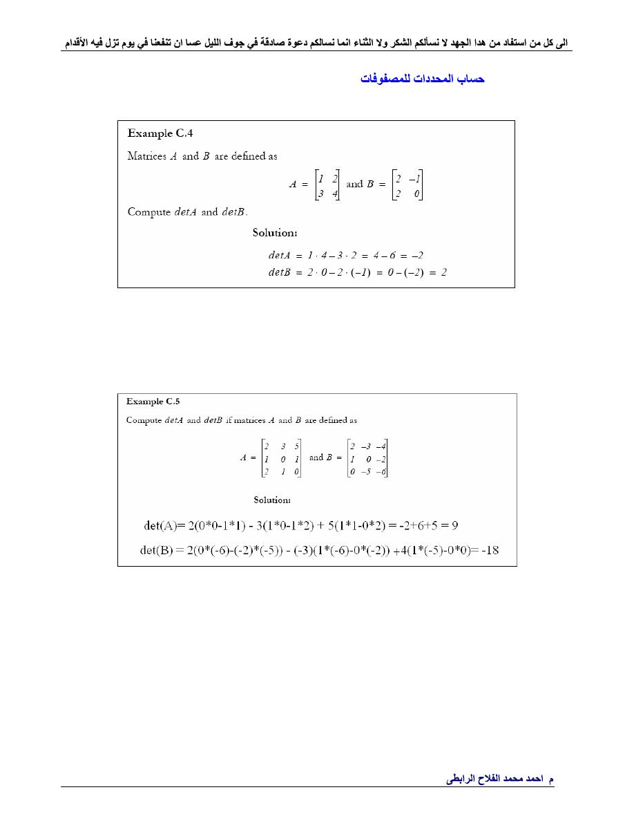
Determinants of Matrices
((
Check with MATLAB:
%----------------------------------------------------------
clc
clear
A=[1 2; 3 4];
B=[2 -1; 2 0];
% Define matrices A and B
det(A)
% Compute the determinant of A
det(B)
% Compute the determinant of B
%-----------------------------------------------------------
Check with MATLAB:
%----------------------------------------------------------
clc
clear
A=[2 3 5; 1 0 1; 2 1 0];
% Define matrix A
B=[2 -3 -4; 1 0 -2; 0 -5 -6];
% Define matrix B
det(A)
% Compute the determinant of A
det(B)
% Compute the determinant of B
%-----------------------------------------------------------
.
Ahmad_engineer21@yahoo.com
3
-
))
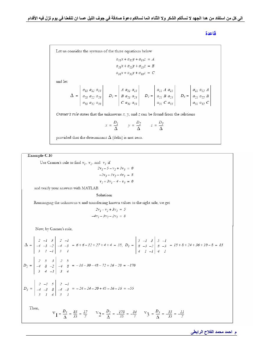
Cramer’s Rule
((
.
Ahmad_engineer21@yahoo.com
We will verify with MATLAB as follows.
%----------------------------------------------------------
clc
clear
% The following code will compute and display the values of v1, v2
and v3.
B=[2 -1 3;-4 -3 -2; 3 1 -1];
% The elements of the determinant
D of matrix B
delta=det(B);
% Compute the determinant D of
matrix B
d1=[5 -1 3; 8 -3 -2; 4 1 -1];
% The elements of D1
detd1=det(d1);
% Compute the determinant of D1
d2=[2 5 3; -4 8 -2; 3 4 -1];
% The elements of D2
detd2=det(d2);
% Compute the determinant of D2
d3=[2 -1 5; -4 -3 8; 3 1 4];
% The elements of D3
detd3=det(d3);
% Compute he determinant of D3
v1=detd1/delta;
% Compute the value of v1
v2=detd2/delta;
% Compute the value of v2
v3=detd3/delta;
% Compute the value of v3
%-----------------------------------------------------------
disp(
'v1='
);disp(v1);
% Display the value of v1
disp(
'v2='
);disp(v2);
% Display the value of v2
disp(
'v3='
);disp(v3);
% Display the value of v3
%-----------------------------------------------------------
-4
))
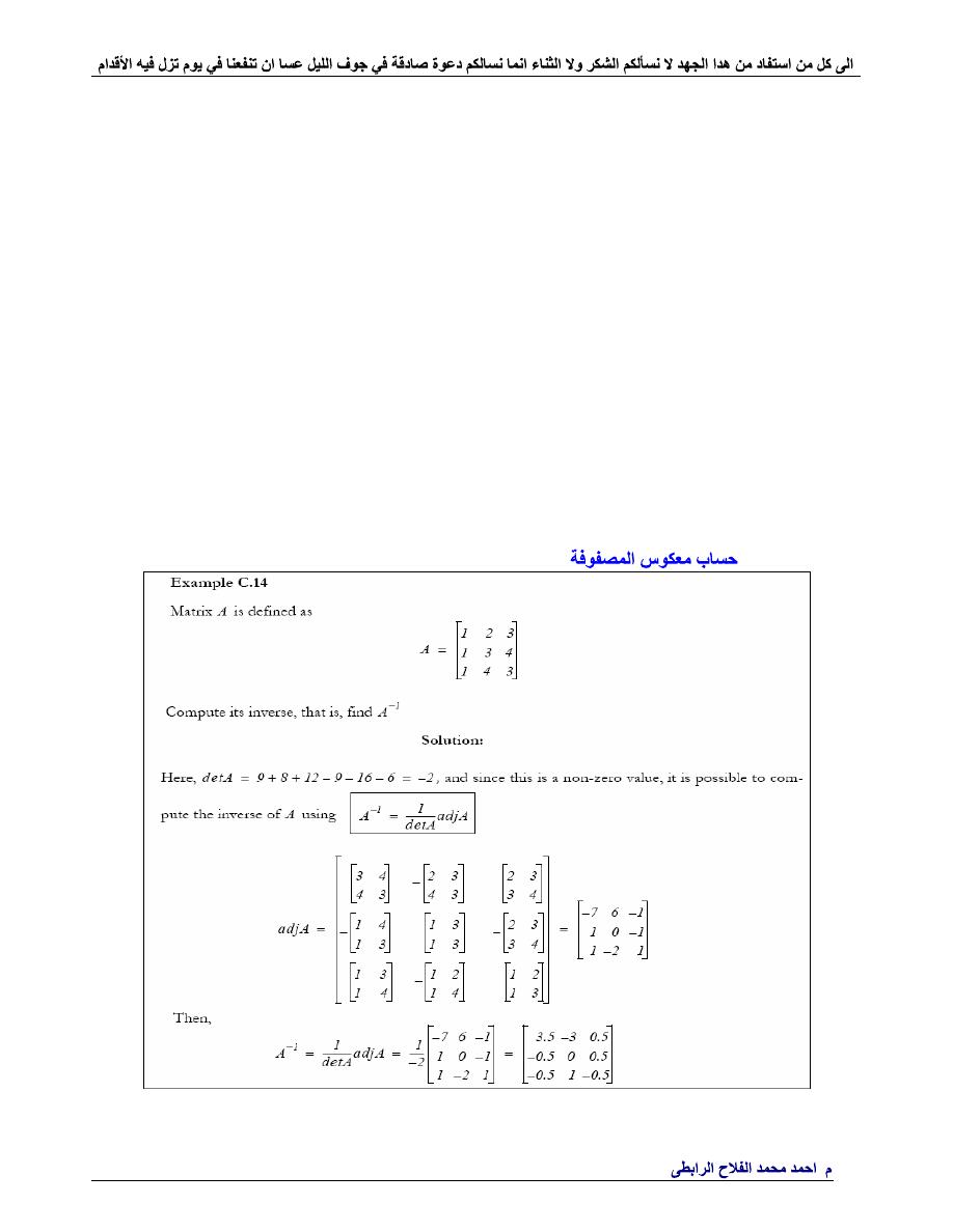
The Inverse of a Matrix
((

.
Ahmad_engineer21@yahoo.com
Check with MATLAB:
%----------------------------------------------------------
clc
clear
A=[1 2 3; 1 3 4; 1 4 3];
invA=inv(A)
%format long;invA
%format short;invA
%-----------------------------------------------------------
.
Ahmad_engineer21@yahoo.com
5
-
))
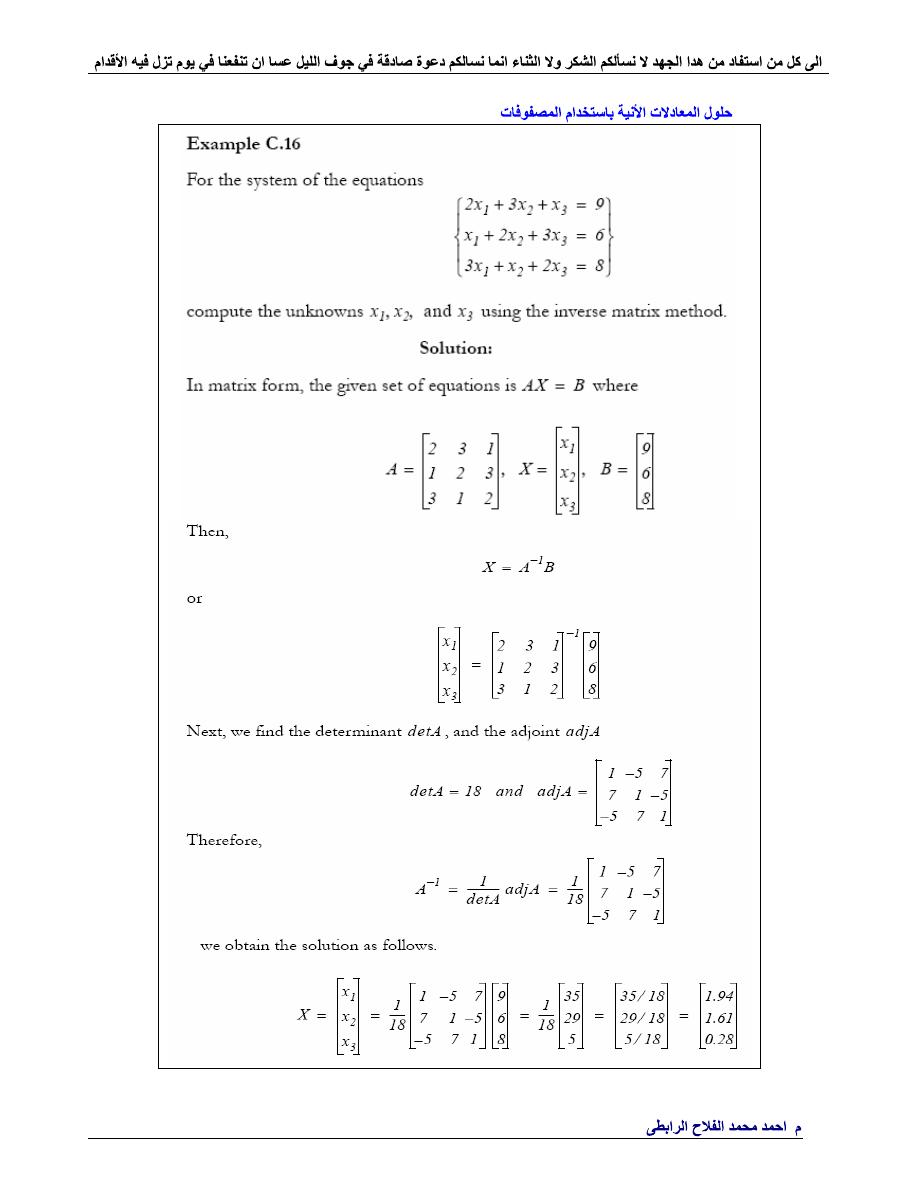
Solution of Simultaneous Equations with Matrices
((

.
Ahmad_engineer21@yahoo.com
Check with MATLAB:
%----------------------------------------------------------
clc
clear
A=[2 3 1; 1 2 3; 3 1 2];
B=[9 6 8]';
X=A\B
M=inv(A)*B
%-----------------------------------------------------------
.
Ahmad_engineer21@yahoo.com

.
Ahmad_engineer21@yahoo.com
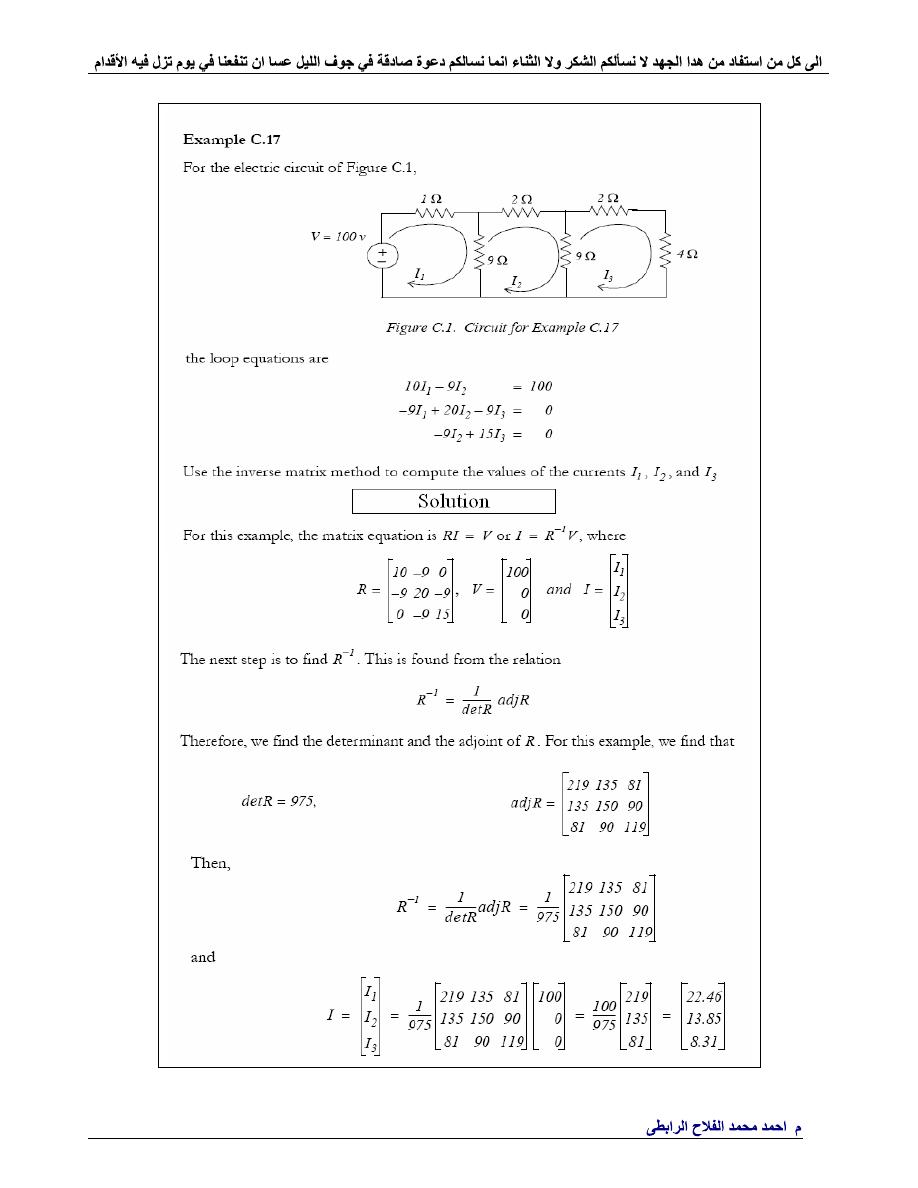
Check with MATLAB:
%----------------------------------------------------------
clc
clear
R=[10 -9 0; -9 20 -9; 0 -9 15];
V=[100 0 0]';
I=R\V;
disp(
'I1='
);
disp(I(1))
disp(
'I2='
);
disp(I(2))
disp(
'I3='
);
disp(I(3))
M=inv(R)*V
%-----------------------------------------------------------
.
Ahmad_engineer21@yahoo.com

.
Ahmad_engineer21@yahoo.com
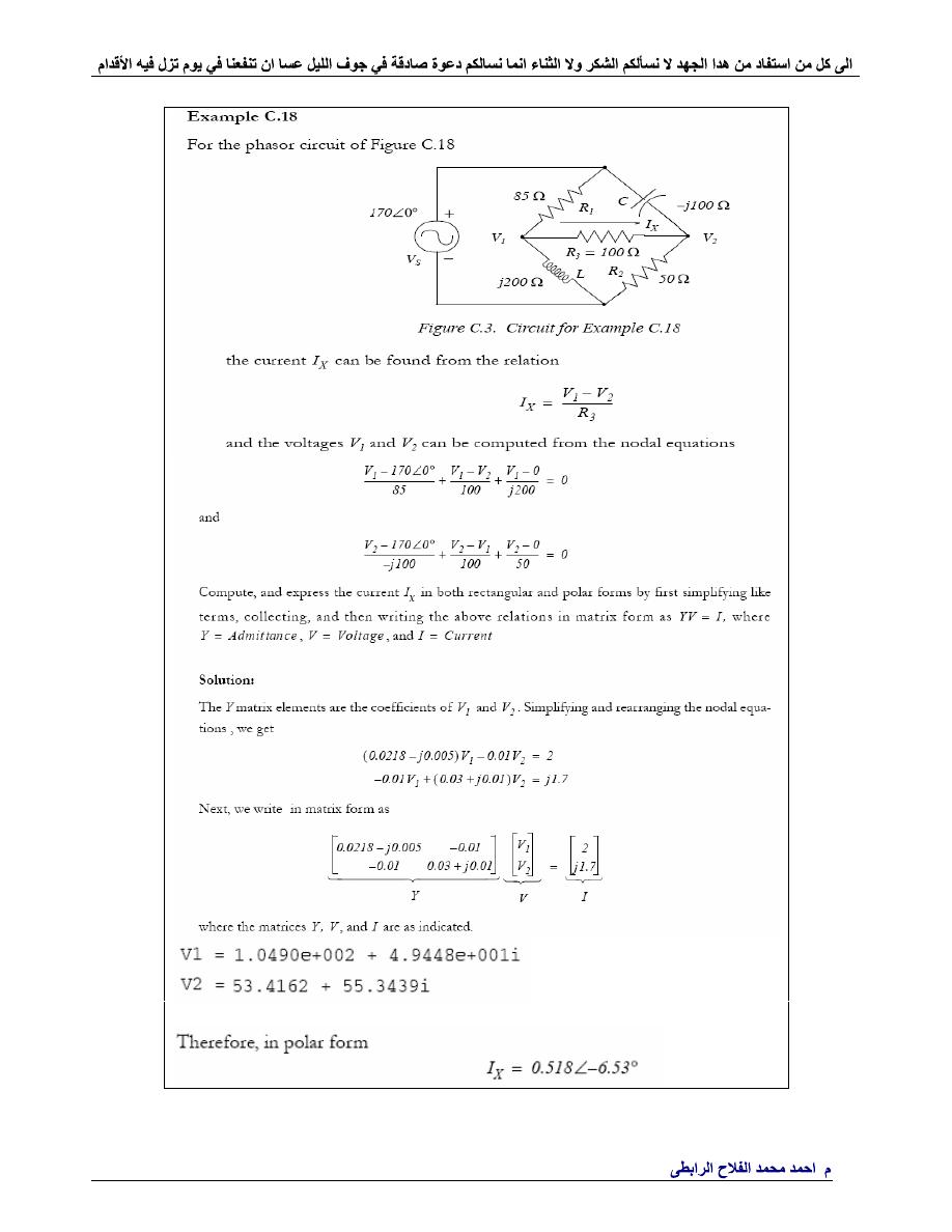
Check with MATLAB:
%----------------------------------------------------------
clc
clear
Y=[0.0218-0.005j -0.01;-0.01 0.03+0.01j];
% Define Y,
I=[2; 1.7j];
% Define I,
V=Y\I;
% Find V
M=inv(Y)*I;
fprintf(
'\n'
);
% Insert a line
disp(
'V1 = '
);
disp(V(1));
% Display values of V1
disp(
'V2 = '
);
disp(V(2));
% Display values of V2
R3=100;
IX=(V(1)-V(2))/R3
% Compute the value of IX
magIX=abs(IX)
% Compute the magnitude
of IX
thetaIX=angle(IX)*180/pi
% Compute angle theta in
degrees
%-----------------------------------------------------------
.
Ahmad_engineer21@yahoo.com
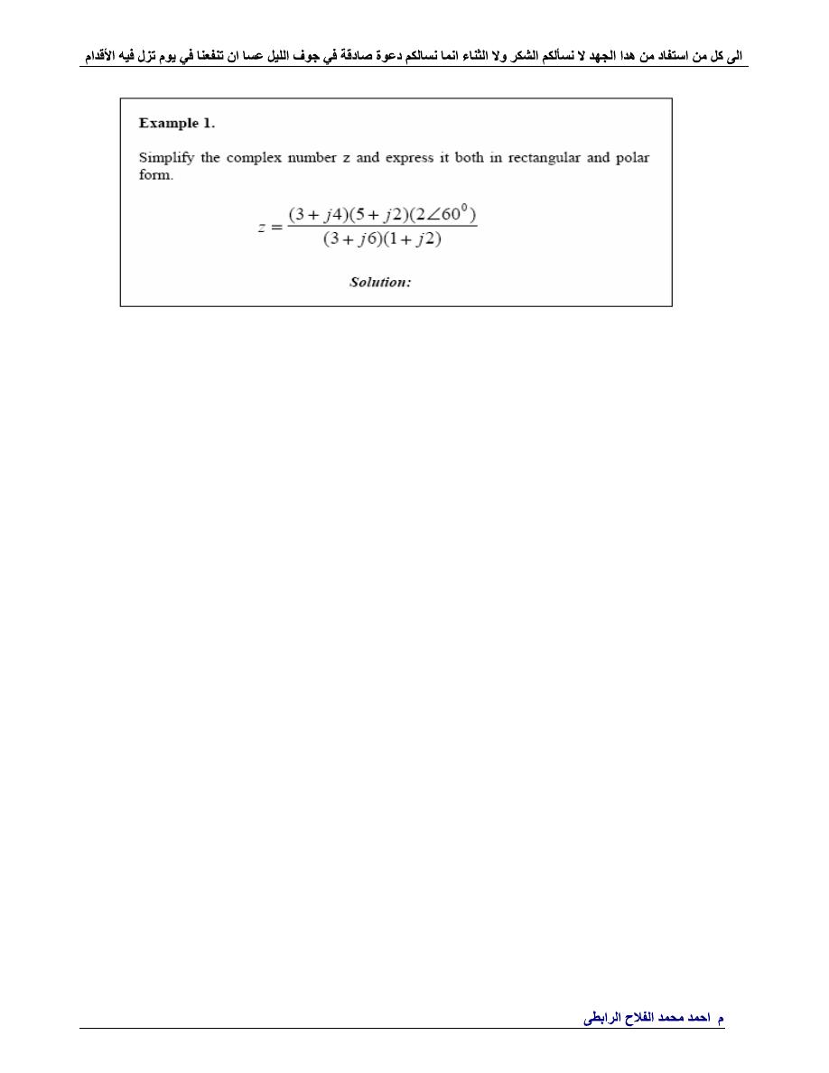
%--------------------------------------------------------------------
% Evaluation of Z
% the complex numbers are entered
%--------------------------------------------------------------------
clc
Z1 = 3+4*j;
Z2 = 5+2*j;
theta = (60/180)*pi;
% angle in radians
Z3 = 2*exp(j*theta);
Z4 = 3+6*j;
Z5 = 1+2*j;
%--------------------------------------------------------------------
% Z_rect is complex number Z in rectangular form
disp(
'Z in rectangular form is'
);
% displays text inside brackets
Z_rect = Z1*Z2*Z3/(Z4+Z5)
Z_mag = abs (Z_rect);
% magnitude of Z
Z_angle = angle(Z_rect)*(180/pi);
% Angle in degrees
disp(
'complex number Z in polar form, mag, phase'
);
% displays text
%inside brackets
Z_polar = [Z_mag, Z_angle]
diary
%--------------------------------------------------------------------

.
Ahmad_engineer21@yahoo.com
%--------------------------------------------------------------------
function
req = equiv_sr(r)
% equiv_sr is a function program for obtaining
% the equivalent resistance of series connected resistors
% usage: req = equiv_sr(r)
% r is an input vector of length n
% req is an output, the equivalent resistance(scalar)
n = length(r);
% number of resistors
req = sum (r);
% sum up all resistors
end
%--------------------------------------------------------------------
The above MATLAB script can be found in the function file
equiv_sr.m,
which is available on the disk that accompanies this book.
Suppose we want to find the equivalent resistance of the series
connected resistors 10, 20, 15, 16 and 5 ohms. The following statements
can be typed in the MATLAB command window to reference the
function
equiv_sr
%---------------------------------------------------------------
clc
a = [10 20 15 16 5];
Rseries = equiv_sr(a)
diary
%----------------------------------------------------------------
The result obtained from MATLAB is
Rseries =
66
.
Ahmad_engineer21@yahoo.com
%-----------------------------------------------------------------
function
rt = rt_quad(coef)
%
% rt_quad is a function for obtaining the roots of
% of a quadratic equation
% usage: rt = rt_quad(coef)
% coef is the coefficients a,b,c of the quadratic
% equation ax*x + bx + c =0
% rt are the roots, vector of length 2
% coefficient a, b, c are obtained from vector coef
a = coef(1); b = coef(2); c = coef(3);
int = b^2 - 4*a*c;
if
int > 0
srint = sqrt(int);
x1= (-b + srint)/(2*a);
x2= (-b - srint)/(2*a);
elseif
int == 0
x1= -b/(2*a);
x2= x1;
elseif
int < 0
srint = sqrt(-int);
p1 = -b/(2*a);
p2 = srint/(2*a);
x1 = p1+p2*j;
x2 = p1-p2*j;
end
rt =[x1;x2];
end
%------------------------------------------------------------------
We can use m-file function, rt_quad, to find the roots of the following
quadratic equations:
%---------------------------------------------------
clc
%diary ex1.dat
ca = [1 3 2];
ra = rt_quad(ca)
cb = [1 2 1];
rb = rt_quad(cb)
cc = [1 -2 3];
rc = rt_quad(cc)
diary
%---------------------------------------------------

.
Ahmad_engineer21@yahoo.com
%----aX^2+bX+c=0-----------------------------------------------------
clear
clc
close
all
a = input(
' a = '
);
b = input(
' b = '
);
c = input(
' c = '
);
x1 = ( - b + sqrt( b^2-4*a*c))/(2*a)
x2 = ( - b + sqrt( b^2-4*a*c))/(2*a)
if
imag(x1)==0 & imag(x2)==0
if
x1==x2
str=
'ident'
else
str=
'real'
end
elseif
real(x1)==0 & real(x2)==0
str=
'imag'
else
str=
'comp'
end
bigstr=[
'(x1='
,num2str(x1),
')--'
,
'(x2='
,num2str(x2),
')--'
,str];
msgbox(bigstr)
%--------------------------------------------------------------------
800
,
120
/
80
/
200
/
%--------------------------------------------------------------------
clear
clc
close
all
a=input(
'enter your transportation method :'
,
's'
);
switch
a
case
'car'
t=800/120
msgbox([
'your trip will take '
,num2str(t),
' hours'
]);
case
'bus'
t=800/80
msgbox([
'your trip will take '
,num2str(t),
' hours'
]);
case
'plane'
t=800/200
msgbox([
'your trip will take '
,num2str(t),
' hours'
]);
otherwise
msgbox(
'inter valed tm'
)
end
%--------------------------------------------------------------------
.
Ahmad_engineer21@yahoo.com
1
-
))
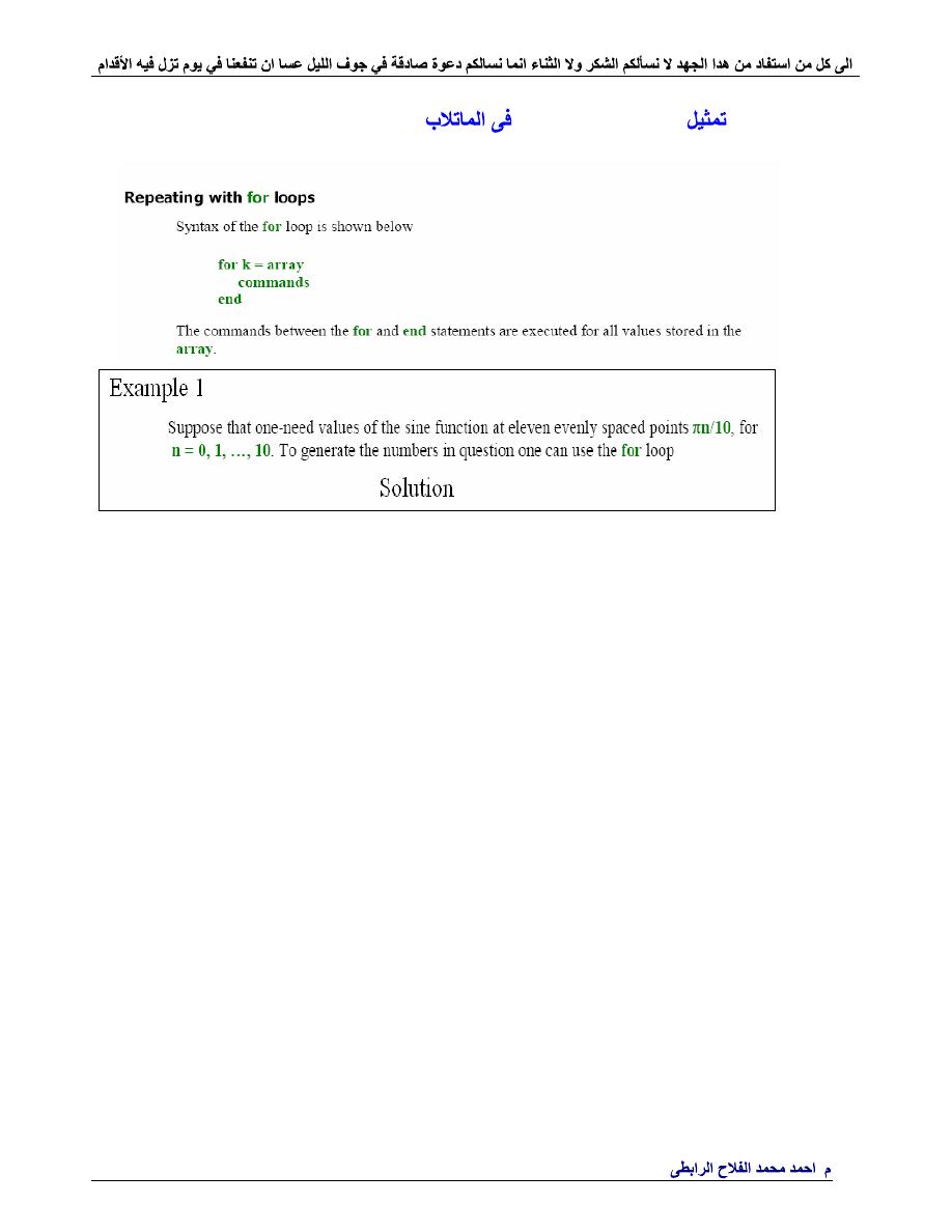
the for loops
((
%------------------------------------------
clc
for
n=0:10
x(n+1) = sin(pi*n/10);
end
x
%----------------------------------------
%------------------------------------------
clc
H = zeros(5);
for
k=1:5
for
l=1:5
H(k,l) = 1/(k+l-1);
end
end
H
%----------------------------------------
%------------------------------------------
clc
A = zeros(10);
for
k=1:10
for
l=1:10
A(k,l) = sin(k)*cos(l);
end
end
%------------------------------------------
k = 1:10;
A = sin(k)'*cos(k);
%------------------------------------------
.
Ahmad_engineer21@yahoo.com
2
-
))
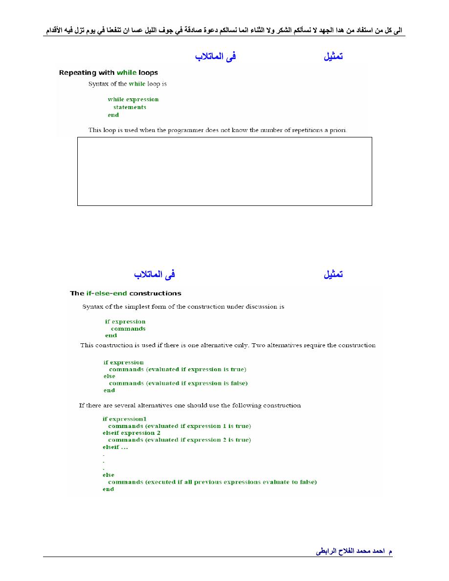
the while loops
((
Example 1
This process is continued till the current quotient is less than or equal
to 0.01. What is the largest quotient that is greater than 0.01?
Solution
%------------------------------------------
clc
q = pi;
while
q > 0.01
q = q/2;
end
q
%------------------------------------------
3
-
))
the if-else-end constructions
((
.
Ahmad_engineer21@yahoo.com
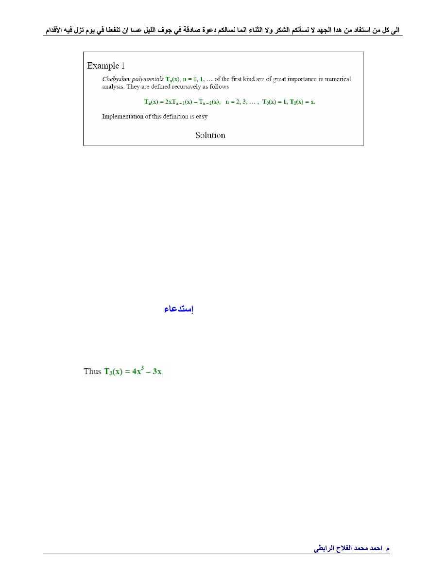
%--------------------------------------------------------
function
T = chebt(n)
% Coefficients T of the nth Chebyshev polynomial of the first
kind.
% They are stored in the descending order of powers.
t0 = 1;
t1 = [1 0];
if
n == 0
T = t0;
elseif
n == 1;
T = t1;
else
for
k=2:n
T = [2*t1 0] - [0 0 t0];
t0 = t1;
t1 = T;
end
end
%---------------------------------------------------------
%---------------------------------------------------------
clc
n=3
coff = chebt(n)
diary
%---------------------------------------------------------
.
Ahmad_engineer21@yahoo.com
4
-
))
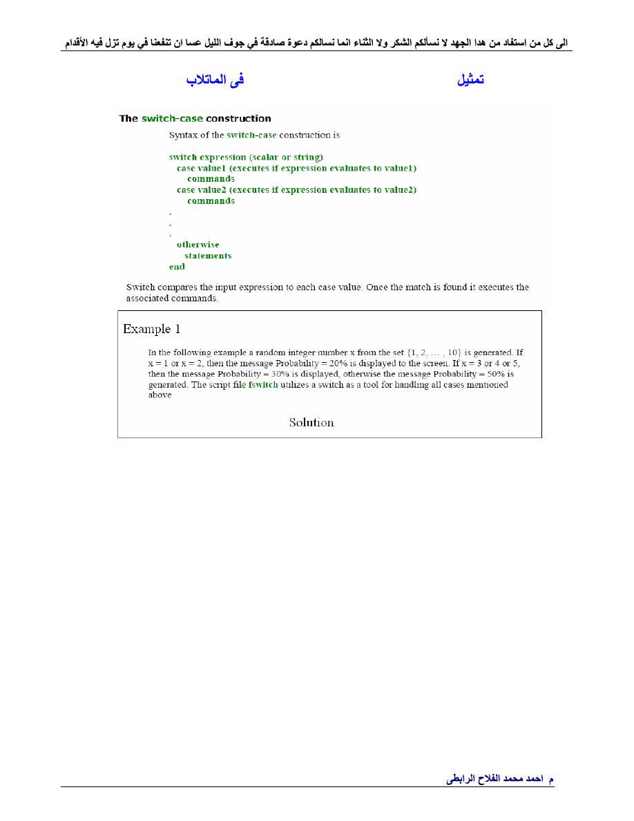
the switch-case constructions
((
%--------------------------------------------------------------------
clc
% Script file fswitch.
x = ceil(10*rand);
% Generate a random integer in {1, 2, ... , 10}
switch
x
case
{1,2}
disp(
'Probability = 20%'
);
case
{3,4,5}
disp(
'Probability = 30%'
);
otherwise
disp(
'Probability = 50%'
);
end
%--------------------------------------------------------------------
Note use of the curly braces{ }after the word
case
. This creates the
so-called cell array rather than the one-dimensional array, which requires
use of the square brackets[].
.
Ahmad_engineer21@yahoo.com
5
-
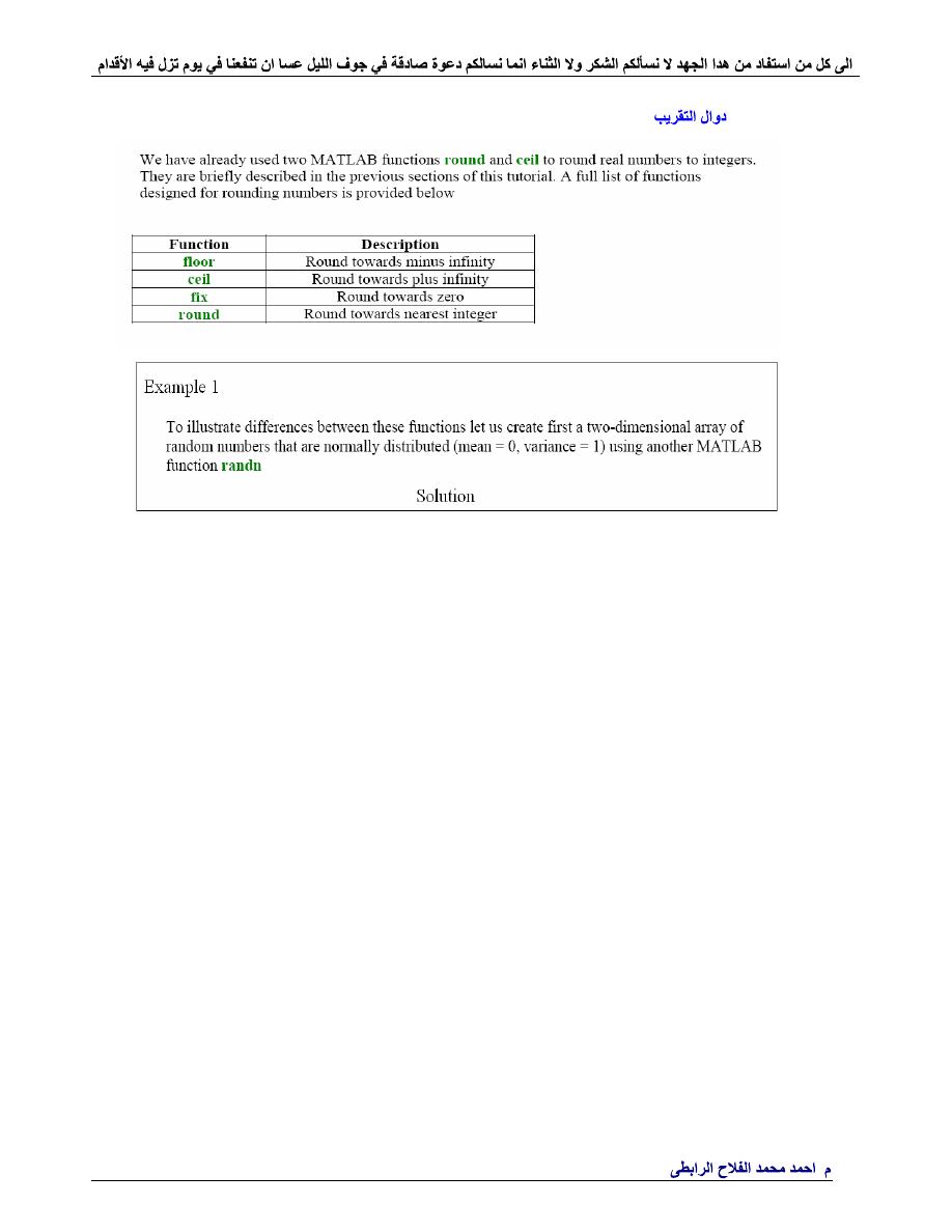
))
Rounding to integers. Function ceil, floor, fix and round
((
%--------------------------------------------------------------------
clc
randn(
'seed'
, 0)
% This sets the seed of the random numbers
% generator to zero
T = randn(5)
A = floor(T)
B = ceil(T)
C = fix(T)
D = round(T)
%--------------------------------------------------------------------

.
Ahmad_engineer21@yahoo.com
%--------------------------------------------------------
function
[m, r] = rep4(x)
% Given a nonnegative number x, function rep4 computes an integer m
% and a real number r, where 0.25 <= r < 1, such that x = (4^m)*r.
if
x == 0
m = 0;
r = 0;
return
end
u = log10(x)/log10(4);
if
u < 0
m = floor(u)
else
m = ceil(u);
end
r = x/4^m;
%-------------------------------------------------------------------
%--------------------------------------------------------------------
clc
[m, r] = rep4(pi)
%--------------------------------------------------------------------
.
Ahmad_engineer21@yahoo.com
11
-
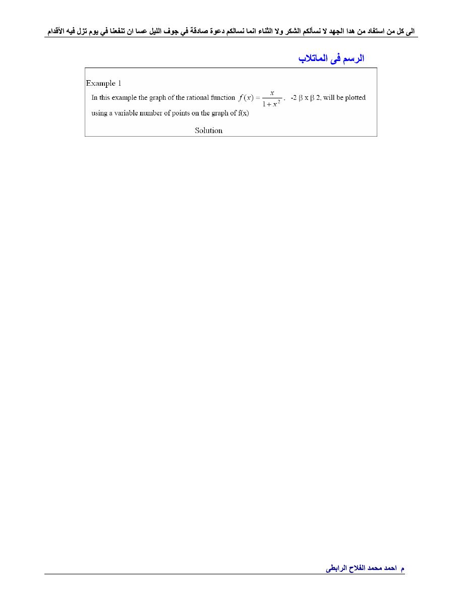
))
((MATLAB graphics
%--------------------------------------------------------------------
clc
% Script file graph1.
% Graph of the rational function y = x/(1+x^2).
for
n=1:2:5
n10 = 10*n;
x = linspace(-2,2,n10);
y = x./(1+x.^2);
plot(x,y,
'r'
)
title(sprintf(
'Graph %g. Plot based upon n = %g points.'
,(n+1)/2, n10))
axis([-2,2,-.8,.8])
xlabel(
'x'
)
ylabel(
'y'
)
grid
pause(3)
end
%--------------------------------------------------------------------
clc
% Script file graph2.
% Several plots of the rational function y = x/(1+x^2)
% in the same window.
k = 0;
for
n=1:3:10
n10 = 10*n;
x = linspace(-2,2,n10);
y = x./(1+x.^2);
k = k+1;
subplot(2,2,k)
plot(x,y,
'r'
)
title(sprintf(
'Graph %g. Plot based upon n = %g points.'
, k, n10))
xlabel(
'x'
)
ylabel(
'y'
)
axis([-2,2,-.8,.8])
grid
pause(3);
end
%--------------------------------------------------------------------
.
Ahmad_engineer21@yahoo.com
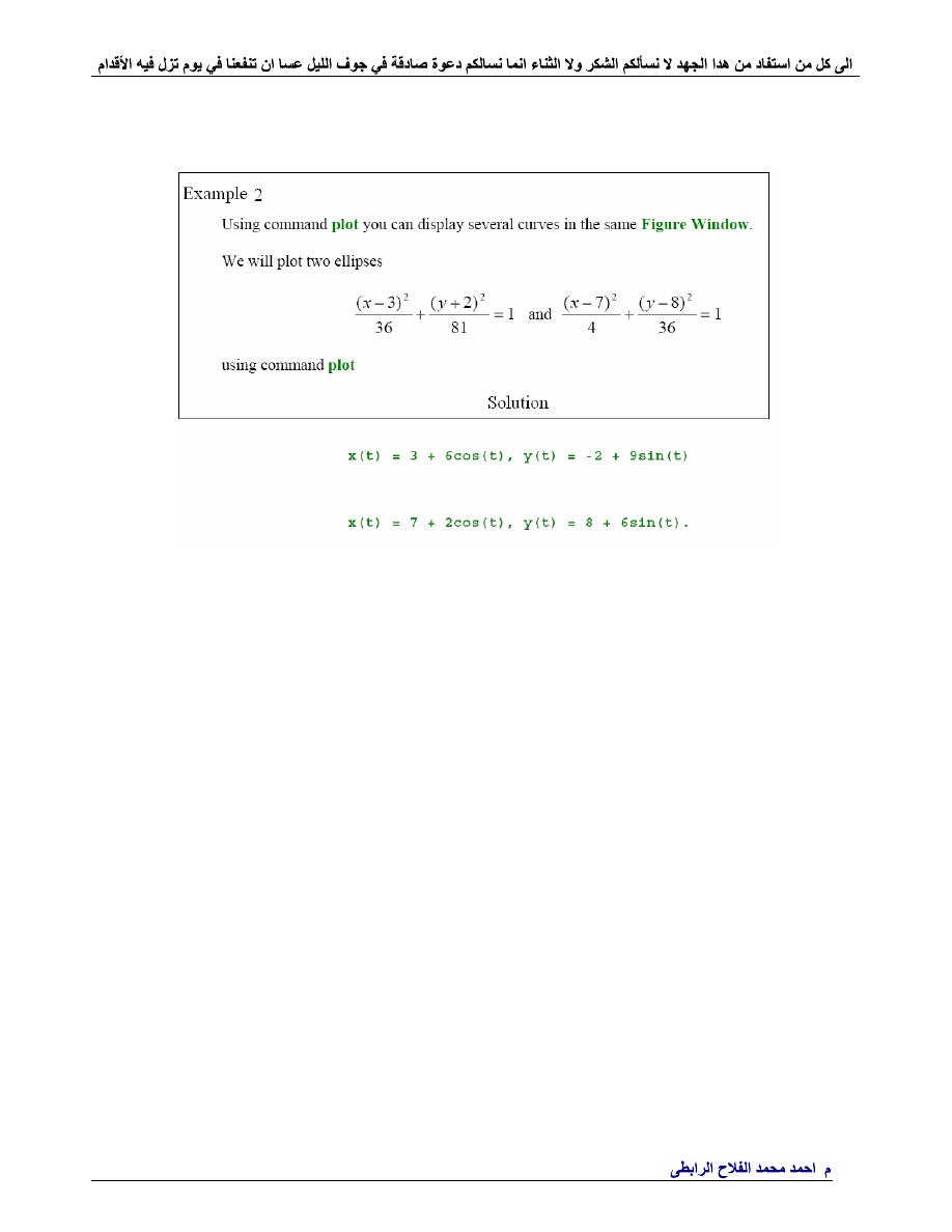
%--------------------------------------------------------------------
clc
% Script file graph3.
% Graphs of two ellipses
% x(t) = 3 + 6cos(t), y(t) = -2 + 9sin(t)
% and
% x(t) = 7 + 2cos(t), y(t) = 8 + 6sin(t).
t = 0:pi/100:2*pi;
x1 = 3 + 6*cos(t);
y1 = -2 + 9*sin(t);
x2 = 7 + 2*cos(t);
y2 = 8 + 6*sin(t);
plot(x1,y1,
'r'
,x2,y2,
'b'
);
axis([-10 15 -14 20])
xlabel(
'x'
)
ylabel(
'y'
)
title(
'Graphs of (x-3)^2/36+(y+2)^2/81 = 1 and (x-7)^2/4+(y-8)^2/36 =1.'
)
grid
%--------------------------------------------------------------------
.
Ahmad_engineer21@yahoo.com
%--------------------------------------------------------------------
clc
t = 0:pi/100:2*pi;
x = cos(t);
y = sin(t);
plot(x,y)
%--------------------------------------------------------------------
% Script file graph4.
% Curve r(t) = < t*cos(t), t*sin(t), t >.
t = -10*pi:pi/100:10*pi;
x = t.*cos(t);
y = t.*sin(t);
plot3(x,y,t);
title(
'Curve u(t) = < t*cos(t), t*sin(t), t >'
)
xlabel(
'x'
)
ylabel(
'y'
)
zlabel(
'z'
)
grid
%--------------------------------------------------------------------
.
Ahmad_engineer21@yahoo.com
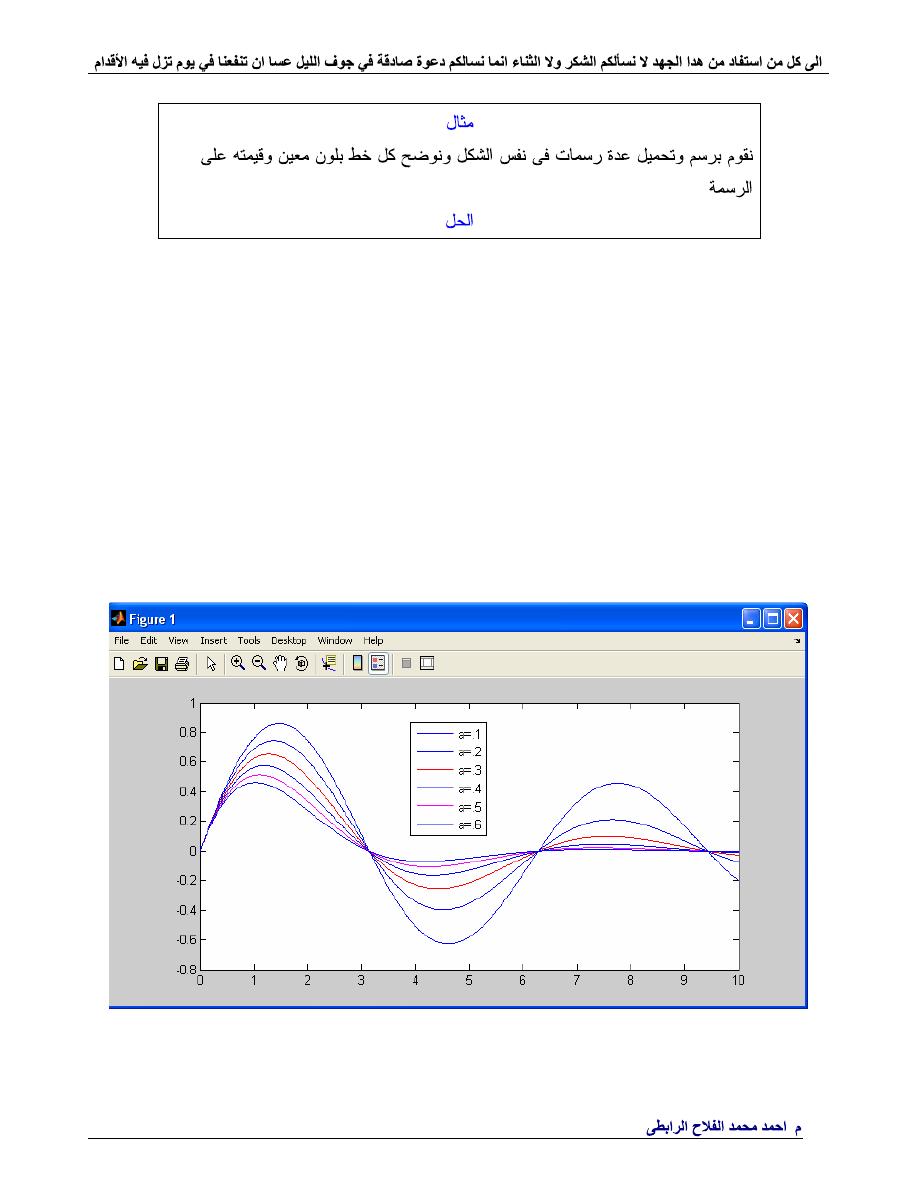
%---------------------------------------------------------------
clear
clc
close
all
x=linspace(0,10,1000);
a=.1:.1:.6;
c=
'b r m c x y'
;
for
i=1:6
y=sin(x).*exp(-a(i)*x);
plot(x,y,c(i))
hold
on
end
legend(
'a=.1'
,
'a=.2'
,
'a=.3'
,
'a=.4'
,
'a=.5'
,
'a=.6'
)
%---------------------------------------------------------------

.
Ahmad_engineer21@yahoo.com
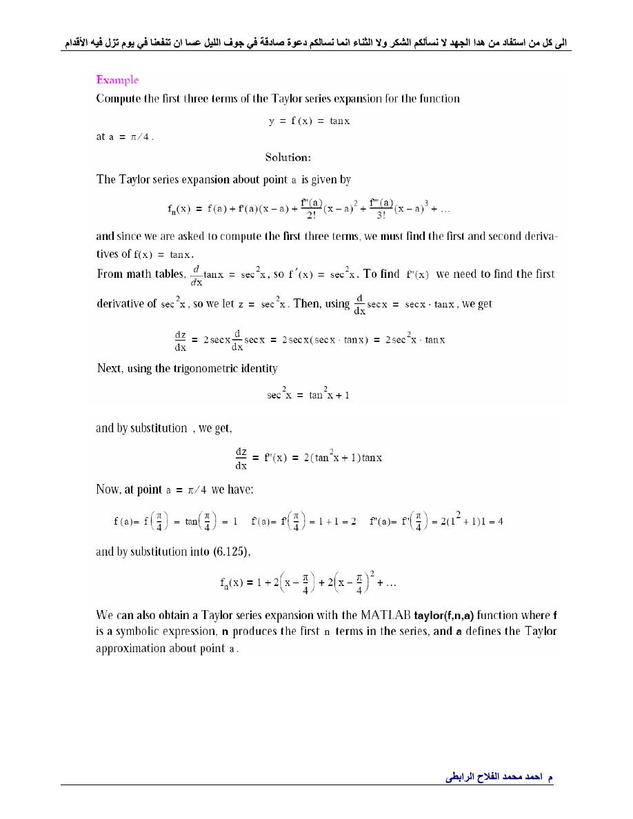
Example
Find first and second derivatives for
F(x)=x^2+2x+2
Solution
%------To find first and second derivatives of Pn(x)-----
--
clc
a=[1 2 3];
syms
x
p=a(1);
for
i=1;
p=a(i+1)+x*p;
end
disp(
'First derivative'
)
p2=p+x*diff(p)
disp(
'Second derivative'
)
p22=diff(p2)
%------------------------------------------------
--
First
derivative
p2 =
2+2*x
Second
derivative
p22 =
2
.
Ahmad_engineer21@yahoo.com
Example
P4(x)=3x^4-10x^3-48x^2-2x+12
at
r=6
deflate the polynomial
with Horners algorithm Find
P3(x).
Solution
%-------------Horner alogorithm------------------
-
clc
a=[3 -10 -48 -2 12];
r=6;
b(1)=a(1);
p=0;
n=length(a);
for
i=2:n;
b(i)=a(i)+r.*b(i-1);
end
syms
x
for
i=1:n;
p=p+b(i)*x^(4-i);
end
disp(
'P3(x)='
)
p
%------------------------------------------------
--
P
3
(x)=
3*x^3+8*x^2-2
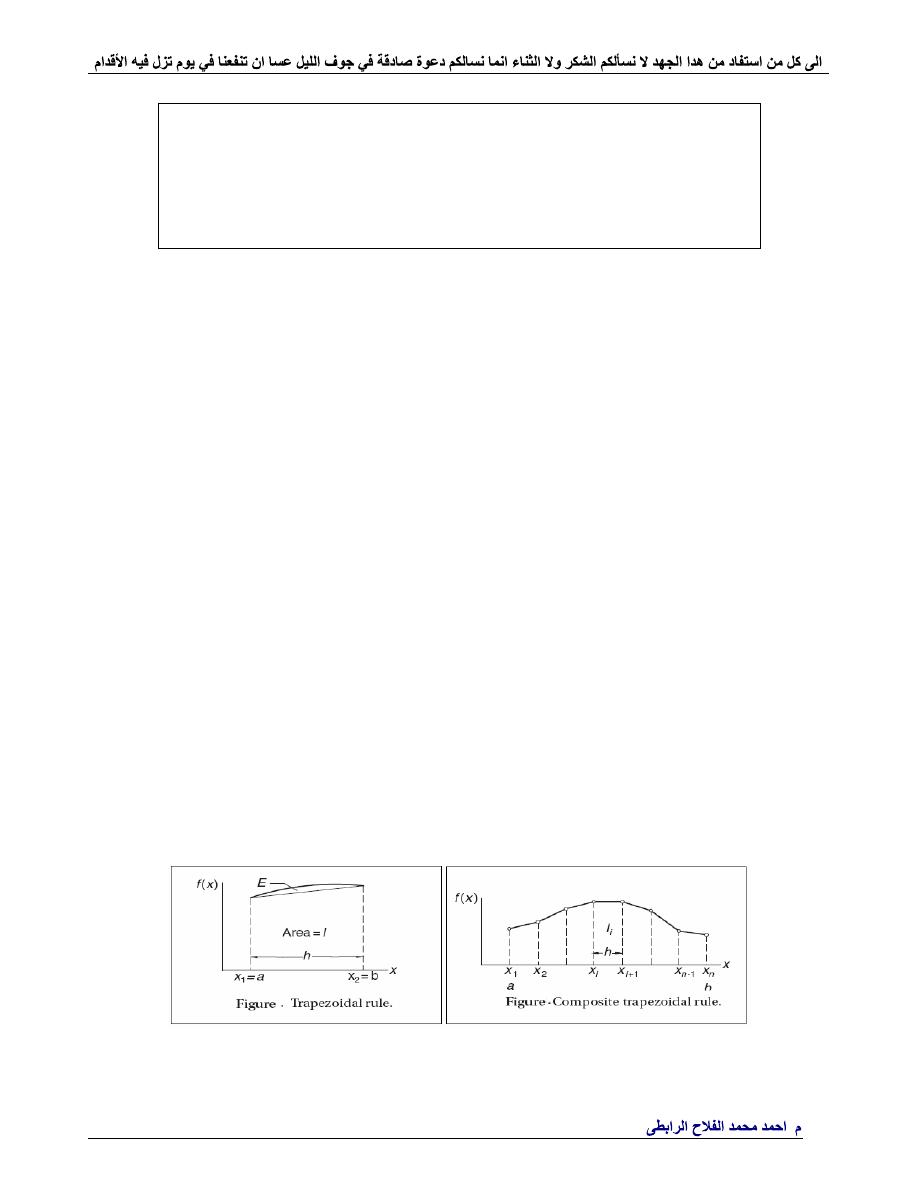
Numerical Integration
1-
Trapezoidal Rule
The composite trapezoidal rule.
.
Ahmad_engineer21@yahoo.com
Example
Suppose we wished to integrate the function trabulated the table
below for
e
x
f
x
)
(
over the interval from x=1.8 to x=3.4 using n=8
b
a
4
3
8
x
.
.
1
)
(
)
(
dx
e
dx
x
f
Am
x
1.6
1.8
2
2.2
2.4
2.6
2.8
3
3.2
3.4
3.6
3.8
f(x)
4.953
6.050
7.389
9.025
11.023
13.464
16.445
20.086
24.533
29.964
36.598
44.701
Solution
%---Trapezoidal Rule---------------
clc
a=1.8;
b=3.4;
h=0.2;
n=(b-a)/h
f=0;
x=2;
for
i=1:n;
%c=a+(i-1/2)*h;
%f=f+(c^2+1);
f=(f+exp(x))
x=x+h;
end
Am_approx=h/2*(exp(a)+2*f+exp(b))
syms
t
Am_exact=int(exp(t),1.8,3.4)
error=Am_exact-Am_approx
E_t=(error/(Am_approx+error))*100
E_a=((Am_approx-Am_exact)/Am_approx)*100
%--------------------------------
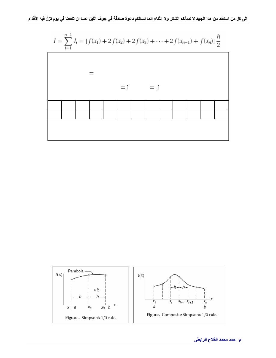
2-
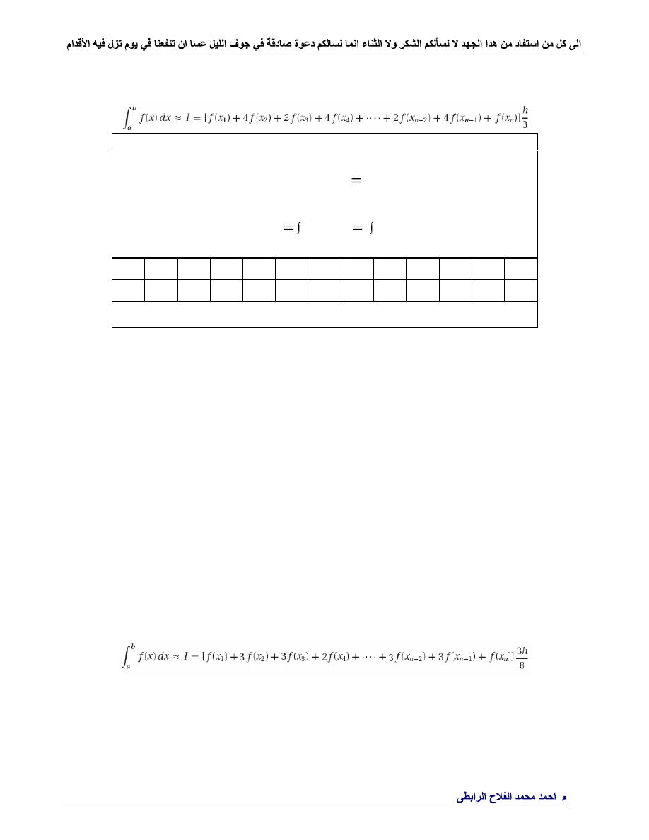
Simpson
’
s 1/3 rule
.
Ahmad_engineer21@yahoo.com
The composite Simpson
’
s 1/3 rule
Example
Suppose we wished to integrate the function using
Simpson
’
s 1/3 rule
and
Simpson
’
s 3/8 rule
the table below for
e
x
f
x
)
(
over the interval from x=1.8
to x=3.4 using n=8
b
a
4
3
8
x
.
.
1
)
(
)
(
dx
e
dx
x
f
Am
x
1.6
1.8
2
2.2
2.4
2.6
2.8
3
3.2
3.4
3.6
3.8
f(x)
4.953
6.050
7.389
9.025
11.023
13.464
16.445
20.086
24.533
29.964
36.598
44.701
Solution
%---Simpson’s 1/3 rule --------------------------------
clc
a=1.8;
b=3.4;
h=0.2;
n=(b-a)/h
f=0;
m=0;
for
x=2:(h+h):3.2;
f=(f+exp(x));
end
for
x=2.2:(h+h):3;
m=(m+exp(x));
end
Am_approx=h/3*(exp(a)+4*f+2*m+exp(b))
syms
t
Am_exact=int(exp(t),1.8,3.4)
error=Am_exact-Am_approx
E_t=(error/(Am_approx+error))*100
E_a=((Am_approx-Am_exact)/Am_approx)*100
%-----------------------------------------------------
3-Simpson
’
s 3/8 rule
The composite Simpson
’
s 3/8 rule
%--------------------Simpson’s 3/8 rule --------------
clc
a=1.8;
b=3.4;

.
Ahmad_engineer21@yahoo.com
h=0.2;
n=(b-a)/h;
f=0;
m=0;
%----------------------------------------------------
for
x=2:h:2+h;
f=f+exp(x)
end
%----------------------------------------------------
x=x+h;
m=exp(x);
%----------------------------------------------------
for
x=2.6:h:2.6+h;
f=f+exp(x);
end
%----------------------------------------------------
x=x+h;
m=m+exp(x);
x=x+h;
f=f+exp(x);
%----------------------------------------------------
Am_approx=((3*h)/8)*(exp(a)+3*f+2*m+exp(b))
%----------------------------------------------------
syms
t
Am_exact=int(exp(t),1.8,3.4)
error=Am_exact-Am_approx
E_t=(error/(Am_approx+error))*100
E_a=((Am_approx-Am_exact)/Am_approx)*100
%----------------------------------------------------
%--------------------Simpson’s 3/8 rule --------------
clc
a=1.8;b=3.4;h=0.2;n=(b-a)/h;f=0;m=0;
%----------------------------------------------------
for
x=2:h:3.2;
switch
x
case
{2,2.2}
f=f+exp(x)

.
Ahmad_engineer21@yahoo.com
case
{2.4}
m=exp(x);
case
{2.6,2.8}
f=f+exp(x);
case
{3}
m=m+exp(x);
otherwise
f=f+exp(x);
end
end
%----------------------------------------------------
Am_approx=((3*h)/8)*(exp(a)+3*(f)+2*(m)+exp(b))
%----------------------------------------------------
syms
t
Am_exact=int(exp(t),1.8,3.4)
pretty(Am_exact)
error=Am_exact-Am_approx
pretty(error)
E_t=(error/(Am_approx+error))*100
pretty(E_t)
E_a=((Am_approx-Am_exact)/Am_approx)*100
pretty(E_a)
%----------------------------------------------------
.
Ahmad_engineer21@yahoo.com
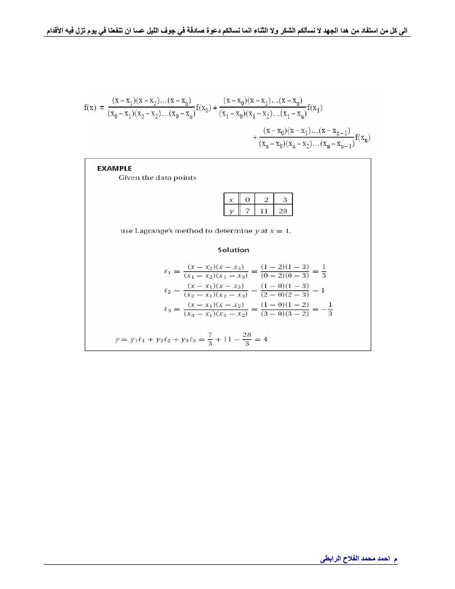
4-Lagrange Interpolating Polynomial Method
Lagrange’s interpolation method uses the formula
%-----------Lagrange’s interpolation method ---------
clc
x=1;
%syms x
%----------------------------------------------------
x1=0;
x2=2;
x3=3;
%----------------------------------------------------
y0=7;
y1=11;
y2=28;
%----------------------------------------------------
l0=((x-x2)*(x-x3))/((x1-x2)*(x1-x3))
l1=((x-x1)*(x-x3))/((x2-x1)*(x2-x3))
l2=((x-x1)*(x-x2))/((x3-x1)*(x3-x2))
%----------------------------------------------------
y=y0*l0+y1*l1+y2*l2
%----------------------------------------------------
.
Ahmad_engineer21@yahoo.com
Example 2
Construct the polynomial interpolating the data by using
Lagrange polynomials
X
1
1/2
3
F(x)
3
-10
2
Solution
%-----------Lagrange’s interpolation method ---------
clc
syms
x
%----------------------------------------------------
x1=1;
x2=0.5;
x3=3;
%----------------------------------------------------
y0=3;
y1=-10;
y2=2;
%----------------------------------------------------
l0=((x-x2)*(x-x3))/((x1-x2)*(x1-x3))
l1=((x-x1)*(x-x3))/((x2-x1)*(x2-x3))
l2=((x-x1)*(x-x2))/((x3-x1)*(x3-x2))
%----------------------------------------------------
y=y0*l0+y1*l1+y2*l2;
collect(y)
%----------------------------------------------------
%-------------Lagrange's interpolation method--------
clc
syms
x
p=0;
s=[1 1/2 3];
f=[3 -10 2];
n=length(s);
for
i=1:n;
l=1;
for
j=1:n;
if
(i~=j);
l=((x-s(j))/(s(i)-s(j)))*l;
end
end
p=l.*f(i)+p;
end
p=collect(p)
%----------------------------------------------------

.
Ahmad_engineer21@yahoo.com
Example 2
Construct the polynomial interpolating the data by using
Lagrange polynomials
X
1
1/2
3
F(x)
3
-10
2
Solution
%-------------Lagrange's interpolation method--------
clc
x=input(
' enter value of x:'
)
p=0;
s=[1 1/2 3];
f=[3 -10 2];
n=length(s);
for
i=1:n;
l=1;
for
j=1:n;
if
(i~=j);
l=((x-s(j))/(s(i)-s(j)))*l;
end
end
p=l.*f(i)+p;
end
p;
fprintf(
'\n p(%3.3f)=%5.4f'
,x,p)
%---------------------------------------------------
syms
x
p=0;
for
i=1:n;
l=1;
for
j=1:n;
if
(i~=j);
l=((x-s(j))/(s(i)-s(j)))*l;
end
end
p=l.*f(i)+p;
end
p=collect(p)
%---------------------------------------------------
p = -283/10 -53/5 *
x
^2 + 419/10 *
x
enter value of
x
:5
x
=5
p(
5.000
)=-83.8000
%---------------------------------------------------

.
Ahmad_engineer21@yahoo.com
Example 3
Find the area by lagrange polynomial using 3 nodes
X
1.8
2.6
3.4
F(x)
6.04964
13.464
29.964
Solution
%-----------Lagrange’s interpolation method ---------
clc
syms
x
%----------------------------------------------------
x1=1.8;
x2=2.6;
x3=3.4;
%----------------------------------------------------
F0=6.04964;
F1=13.464;
F2=29.964;
%----------------------------------------------------
l0=((x-x2)*(x-x3))/((x1-x2)*(x1-x3))
A0=int(l0,1.8,3.4)
l1=((x-x1)*(x-x3))/((x2-x1)*(x2-x3))
A1=int(l1,1.8,3.4)
l2=((x-x1)*(x-x2))/((x3-x1)*(x3-x2))
A2=int(l2,1.8,3.4)
%----------------------------------------------------
F=F0*A0+F1*A1+F2*A2
collect(F)
%----------------------------------------------------
%-------------Lagrange's interpolation method---
clc
syms
x
format
long
p=0;
s=[1.8 2.6 3.4];
f=[6.04964 13.464 29.964];
n=length(s);
for
i=1:n;
l=1;
for
j=1:n;
if
(i~=j);
l=((x-s(j))/(s(i)-s(j)))*l;
end
end
A=int(l,s(1),s(n))
p=A*f(i)+p
;
end
p
%-----------------------------------------------
.
Ahmad_engineer21@yahoo.com
5-Mid Point Rule
Example
Find the mid point approximation for
b
a
2
1
)
1
2
^
(
)
(
dx
x
dx
x
f
Am
using n=6
Solution
%---Mid Point Rule---------------
clc
a=-1;
b=2;
n=6;
h=(b-a)/n;
f=0;
for
i=1:n;
c=a+(i-1/2)*h;
f=f+(c^2+1);
end
Am=h*f
%--------------------------------
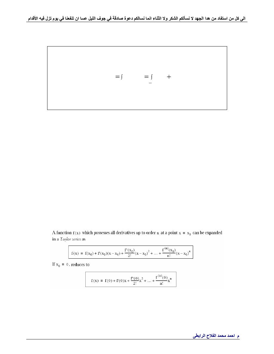
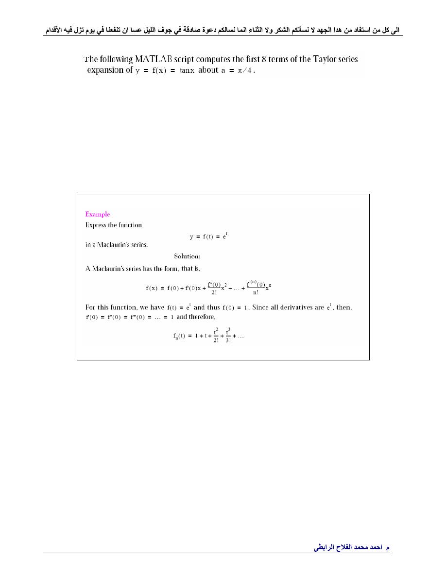
6- Taylor series
.
Ahmad_engineer21@yahoo.com
.
Ahmad_engineer21@yahoo.com
%-------------------- Taylor series --------------
clc
a=pi/4;
sym
x
y=tan(x);
z=taylor(y,8,a);
pretty(z)
%----------------------------------------------------
MATLAB displays the same result.
%-------------------- Taylor series --------------
clc
syms
t
fn=taylor(exp(t));
pretty(fn)
%----------------------------------------------------
.
Ahmad_engineer21@yahoo.com
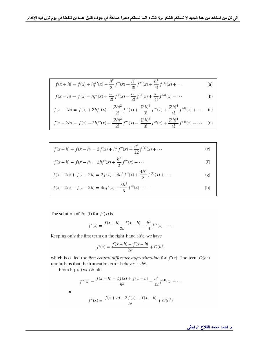
Numerical Differentiation
1-
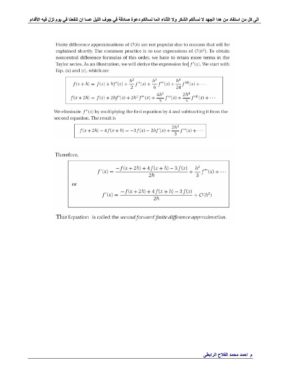
Finite Difference Approximations
The derivation of the finite difference approximations for the derivatives of f (x)
are based on forward and backward Taylor series expansions of f (x) about x,
such as
We also record the sums and differences of the series:
First Central Difference Approximations
.
Ahmad_engineer21@yahoo.com
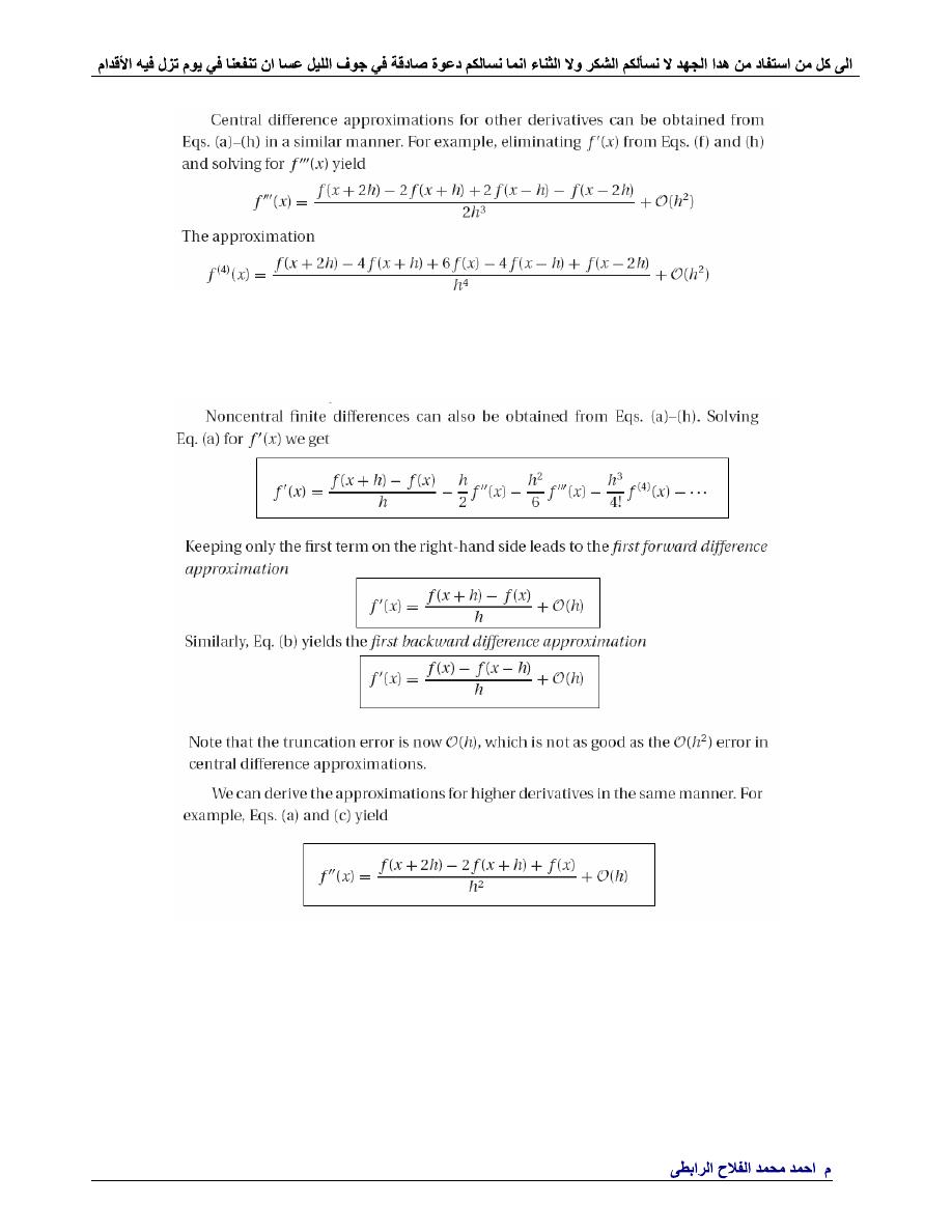
First Noncentral Finite Difference Approximations
These expressions are called
forward
and
backward
finite difference
approximations.
.
Ahmad_engineer21@yahoo.com
Second Noncentral Finite Difference Approximations

.
Ahmad_engineer21@yahoo.com
EXAMPLE
Use forward difference approximations of oh to estimate the first
% derivative of
fx = -0.1.*x.^4-0.15.*x.^3-0.5.*x.^2-0.25.*x+1.2
solution
%---------------------------------------------------------------
% Use forward difference approximations to estimate the first
% derivative of fx=-0.1.*x.^4-0.15.*x.^3-0.5.*x.^2-0.25.*x+1.2
clc
h=0.5;
x=0.5;
x1=x+h
fxx=[-0.1 -0.15 -0.5 -0.25 1.2]
fx=polyval(fxx,x)
fx1=polyval(fxx,x1)
tr_va=polyval(polyder(fxx),0.5)
fda=(fx1-fx)/h
et=(tr_va1-fda)/(tr_va1)*100
%----------------------------------------------------------------
.
Ahmad_engineer21@yahoo.com
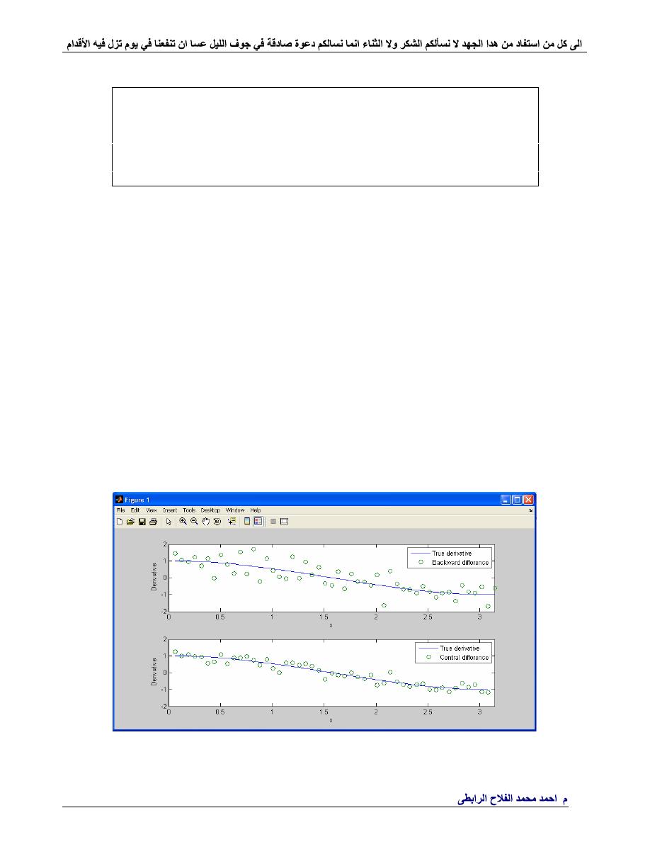
EXAMPLE
Comparison of numerical derivative for backward difference and central
difference method with true derivative and with standard deviation of 0.025
x = [0:pi/50:pi];
yn = sin(x)+0.025
True derivative=td=cos(x)
solution
%--------------------------------------------------------
clc
% Comparison of numerical derivative algorithms
x = [0:pi/50:pi];
n = length(x);
% Sine signal with Gaussian random error
yn = sin(x)+0.025*randn(1,n);
% Derivative of noiseless sine signal
td = cos(x);
% Backward difference estimate noisy sine signal
dynb = diff(yn)./diff(x);
subplot(2,1,1)
plot(x(2:n),td(2:n),x(2:n),dynb,
'o'
)
xlabel(
'x'
)
ylabel(
'Derivative'
)
axis([0 pi -2 2])
legend(
'True derivative'
,
'Backward difference'
)
% Central difference
dync = (yn(3:n)-yn(1:n-2))./(x(3:n)-x(1:n-2));
subplot(2,1,2)
plot(x(2:n-1),td(2:n-1),x(2:n-1),dync,
'o'
)
xlabel(
'x'
)
ylabel(
'Derivative'
)
axis([0 pi -2 2])
legend(
'True derivative'
,
'Central difference'
)
%--------------------------------------------------------
Figure. Comparison of backward difference and central difference methods
.
Ahmad_engineer21@yahoo.com
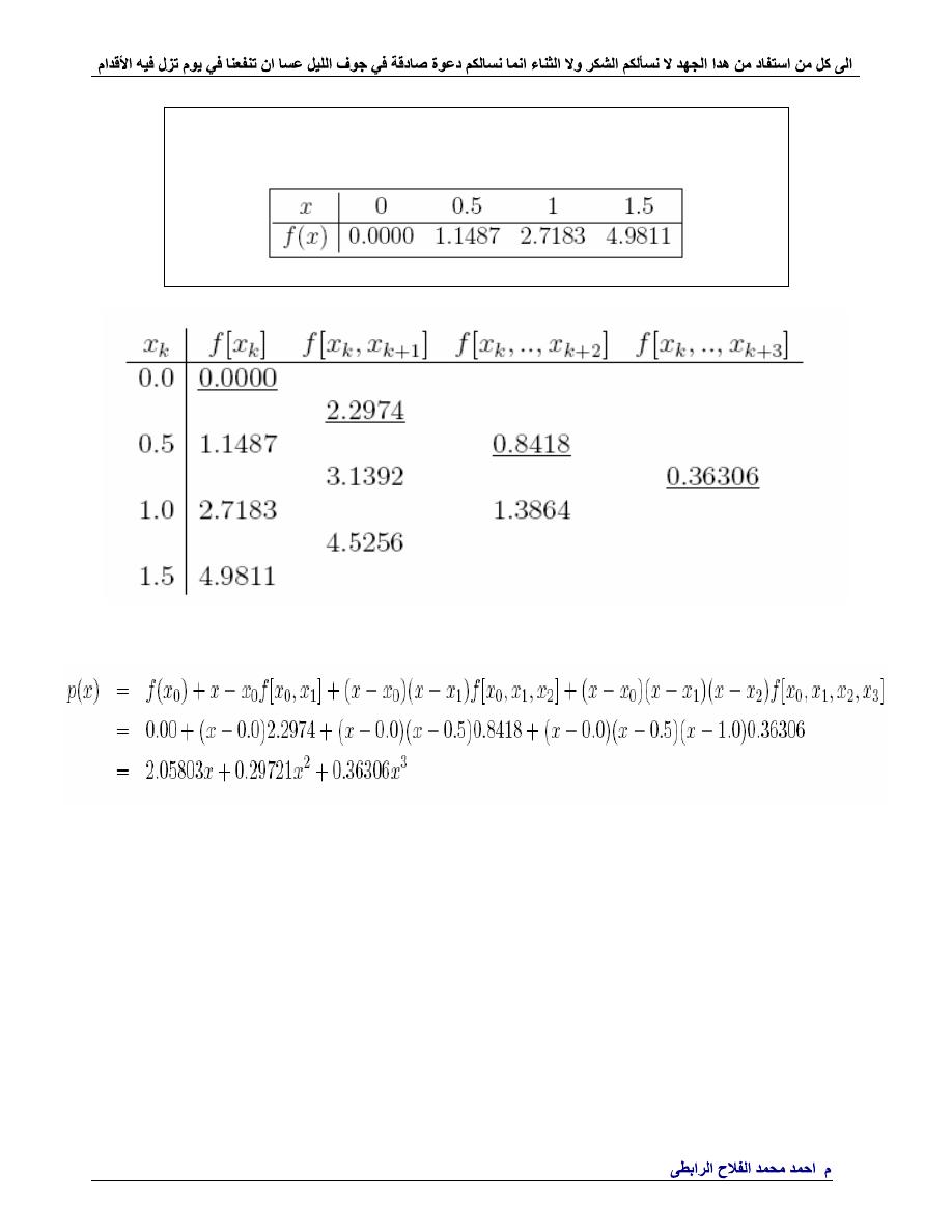
Example
Consider a
Divided Difference table
for points following
Solution

.
Ahmad_engineer21@yahoo.com
%----------------
Divided Difference table algorithm
-------------
clc
disp(
'******** divided difference table *********'
)
x=[2 4 6 8 10]
y=[4.077 11.084 30.128 81.897 222.62]
f00=y(1);
for
i=1:4
f1(i)=(y(i+1)-y(i))/(x(i+1)-x(i));
f01=f1(1);
end
f1=[f1(1) f1(2) f1(3) f1(4)]
for
i=1:3
f2(i)=(f1(i+1)-f1(i))/(x(i+2)-x(i));
f02=f2(1);
end
f2=[f2(1) f2(2) f2(3)]
for
i=1:2
f3(i)=(f2(i+1)-f2(i))/(x(i+3)-x(i));
f03=f3(1);
end
f3=[f3(1) f3(2)]
disp(
'*************************************'
)
y=input(
'enter value of y:'
)
p4x=f00+((y-x(1))*f01)+((y-x(1))*(y-x(2))*f02+((y-x(1))*(y-
x(2))*f02))
fprintf(
'\np4(%3.3f)=%5.4f'
,y,p4x)
syms
y
p4x=f00+((y-x(1))*f01)+((y-x(1))*(y-x(2))*f02+((y-x(1))*(y-
x(2))*f02))
%-------------------------------------------------------------------
f1 = 3.5035 9.5220 25.8845 70.3615
f2 = 1.5046 4.0906 11.1193
f3 = 0.4310 1.1714
p4x = -293/100+7007/2000*y+12037/4000*(y-2)*(y-4)
enter value of y:8
y = 8
p4(8.000)=97.3200
% -------------------------------------------------------------------
.
Ahmad_engineer21@yahoo.com
Example { H.W }
Find the divided differences (newten's Interpolating) for the data
and compare with lagrange interpolating.
X
1
1/2
3
F(x)
3
-10
2
Solution
************** divided difference table *****************
f1 =
26.000000000000000 4.800000000000000
f2 =
-10.600000000000000
----------------Divided Difference table algorithm-------
----------------{ newtens Interpolating }----------------
enter value of y:5
p4(5.000)=-83.8000
px = -283/10-53/5*y^2+419/10*y
----------------------compare with ----------------------
-------------Lagranges interpolation method--------------
enter value of x:5
p(5.000)=-83.8000
p = -283/10-53/5*m^2+419/10*m

.
Ahmad_engineer21@yahoo.com
%------------------------Solve H.W------------------------------
%----------------Divided Difference table algorithm-------------
%----------------{ newten's Interpolating }---------------------
clc
disp(
'******** divided difference table *********'
)
x=[1 0.5 3];
y=[3 -10 2];
f00=y(1);
for
i=1:2;
f1(i)=(y(i+1)-y(i))/(x(i+1)-x(i));
f01=f1(1);
end
f1=[f1(1) f1(2)]
for
i=1;
f2(i)=(f1(i+1)-f1(i))/(x(i+2)-x(i));
f02=f2(1);
end
f2=f2(1)
disp(
'----------------Divided Difference table algorithm-----------'
)
disp(
'----------------{ newtens Interpolating }--------------------'
)
y=input(
'enter value of y:'
);
px=f00+((y-x(1))*f01)+((y-x(1))*(y-x(2))*f02);
fprintf(
'\npx(%3.3f)=%5.4f'
,y,px)
syms
y
px=f00+((y-x(1))*f01)+((y-x(1))*(y-x(2))*f02);
px=collect(px)
%----------------------compare with ---------------------------
%-------------Lagrange's interpolation method------------------
disp(
'----------------------compare with --------------------------'
)
disp(
'-------------Lagranges interpolation method------------------'
)
m=input(
' enter value of x:'
);
p=0;
s=[1 1/2 3];
f=[3 -10 2];
n=length(s);
for
i=1:n;
l=1;
for
j=1:n;
if
(i~=j);
l=((m-s(j))/(s(i)-s(j)))*l;
end
end
p=l.*f(i)+p;
end
p;
fprintf(
'\n p(%3.3f)=%5.4f'
,m,p)
syms
m
p=0;
for
i=1:n;
l=1;
for
j=1:n;
if
(i~=j);
l=((m-s(j))/(s(i)-s(j)))*l;
end
end
p=l.*f(i)+p;
end
p=collect(p)
%--------------------------------------------------------------

.
Ahmad_engineer21@yahoo.com
Example { H.W }
Estimate the In(3) for
Xi
2
4
6
F(x)
In(2)
In(4)
In(6)
a) Linear Interpolation
.
B) Quardratic Interpolation
compare between a&b
Solution
a)Linear Interpolation
.
F1(x)=f(x0)+((f(x1)-f(x0))/(x1-x0))*(x-x0)
b)Quardratic Interpolation
f2(x)=b0+b1*(x-x0)+b2*(x-x0)*(x-x1)
b0= f(x0) = 0.693147180559945;
b1= (f(x1)-f(x0))/(x1-x0) = 0.346573590279973
b2= ((f(x2)-f(x1))/(x2-x1))-b1/(x2-x0) = -0.035960259056473;
---------a) Linear Interpolation---------------------
fx1 = 0.693147180559945-0.346573590279973 (
X
-2)
inter value x:3
fx1 = 1.039720770839918
---------b) Quardratic Interpolation-----------------
fx2 = 0.346573590279973
X
+(-0.035960259056473
X
+0.071920518112945)*(
X
-4)
inter value x:3
fx2 = 1.075681029896391
---------- compare between a&b----------------------
---------a) Linear Interpolation---------------------
Et1 =5.360536964281382 %
---------b) Quardratic Interpolation-----------------
Et2 = 2.087293124994937 %
Quardratic Interpolation is better than Linear Interpolation

.
Ahmad_engineer21@yahoo.com
%---------- Solve H.W-------------------------------------------
%---------a) Linear Interpolation------------------------------
%---------b) Quardratic Interpolation------------------------
%---------- compare between a&b----------------------------
clc
x=input(
'inter value x:'
);
format
long
xi=[2 4 6];
fx=[log(2) log(4) log(6)];
disp(
'---------a) Linear Interpolation-----------------------'
)
fx1=fx(1)+((fx(2)-fx(1))/(xi(2)-xi(1)))*(x-xi(1))
disp(
'---------b) Quardratic Interpolation-----------------'
)
b0=fx(1);
b1=(fx(2)-fx(1))/(xi(2)-xi(1));
b2=(((fx(3)-fx(2))/(xi(3)-xi(2)))-b1)/(xi(3)-xi(1));
fx2=b0+b1*(x-xi(1))+b2*(x-xi(1))*(x-xi(2));
% pretty(fx2)%expand(fx2)%collect(fx2)
disp(
'---------- compare between a&b----------------------'
)
Tv=log(3);
disp(
'---------a) Linear Interpolation-----------------------'
)
Et1=abs((Tv-fx1)/Tv)*100
disp(
'---------b) Quardratic Interpolation-----------------'
)
Et2=abs((Tv-fx2)/Tv)*100
if
Et1>Et2;
disp(
'Quardratic Interpolation is better than Linear Interpolation'
)
else
disp(
'Linear Interpolation is better than Quardratic Interpolation'
)
end
syms
x
disp(
'---------a) Linear Interpolation-----------------------'
)
fx1=fx(1)+((fx(2)-fx(1))/(xi(2)-xi(1)))*(x-xi(1))
disp(
'---------b) Quardratic Interpolation-----------------'
)
b0=fx(1);
b1=(fx(2)-fx(1))/(xi(2)-xi(1));
b2=(((fx(3)-fx(2))/(xi(3)-xi(2)))-b1)/(xi(3)-xi(1));
fx2=b0+b1*(x-xi(1))+b2*(x-xi(1))*(x-xi(2))
.
Ahmad_engineer21@yahoo.com
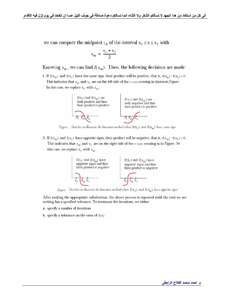
The Bisection Method for Root Approximation
.
Ahmad_engineer21@yahoo.com
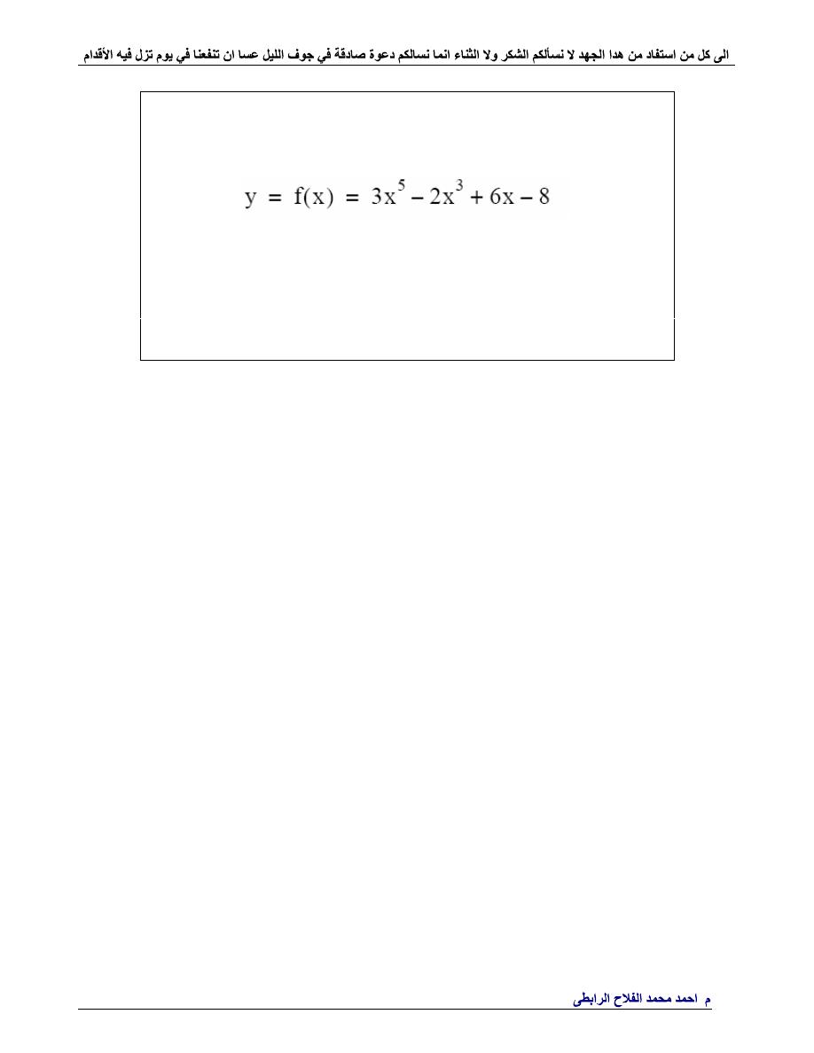
Example
Use the Bisection Method with MATLAB to approximate one of
the roots of
by
a
. by specifying 16 iterations, and using a for end loop MATLAB
program
b
. by specifying 0.00001 tolerance for f(x), and using a while end loop
MATLAB program
Solution:
%--------------------------------------------------------------------
function
y= funcbisect01(x);
y = 3 .* x .^ 5 - 2 .* x .^ 3 + 6 .* x - 8;
% We must not forget to type the semicolon at the end of the line
above;
% otherwise our script will fill the screen with values of y
%--------------------------------------------------------------------
call for function under name funcbisect01.m
%--------------------------------------------------------------------
clc
x1=1;
x2=2;
disp(
'-------------------------'
)
disp(
' xm fm'
)
% xm is the average of x1 and x2, fm is
f(xm)
disp(
'-------------------------'
)
% insert line under xm and
fm
for
k=1:16;
f1=funcbisect01(x1); f2=funcbisect01(x2);
xm=(x1+x2) / 2; fm=funcbisect01(xm);
fprintf(
'%9.6f %13.6f \n'
, xm,fm)
% Prints xm and fm on same
line;
if
(f1*fm<0)
x2=xm;
else
x1=xm;
end
end
disp(
'-------------------------'
)
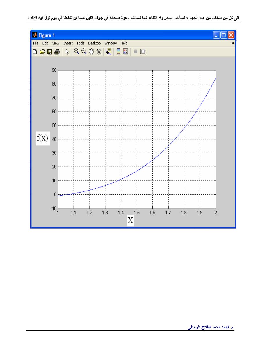
x=1:0.05:2;
y = 3 .* x .^ 5 - 2 .* x .^ 3 + 6 .* x - 8;
plot(x,y)
grid
%--------------------------------------------------------------------
.
Ahmad_engineer21@yahoo.com

.
Ahmad_engineer21@yahoo.com
%--------------------------------------------------------------------
function
y= funcbisect01(x);
y = 3 .* x .^ 5 - 2 .* x .^ 3 + 6 .* x - 8;
% We must not forget to type the semicolon at the end of the line
above;
% otherwise our script will fill the screen with values of y
%--------------------------------------------------------------------
call for function under name funcbisect01.m
%--------------------------------------------------------------------
%--------------------------------------------------------------------
clc
x1=1;
x2=2;
tol=0.00001;
disp(
'-------------------------'
)
disp(
' xm fm'
);
disp(
'-------------------------'
)
while
(abs(x1-x2)>2*tol);
f1=funcbisect01(x1);
f2=funcbisect01(x2);
xm=(x1+x2)/2;
fm=funcbisect01(xm);
fprintf(
'%9.6f %13.6f \n'
, xm,fm);
if
(f1*fm<0);
x2=xm;
else
x1=xm;
end
end
disp(
'-------------------------'
)
%--------------------------------------------------------------------
-------------------------
xm
fm
-------------------------
1.500000 17.031250
1.250000 4.749023
1.125000 1.308441
1.062500 0.038318
1.031250 -0.506944
1.046875 -0.241184
1.054688 -0.103195
1.058594 -0.032885
1.060547 0.002604
1.059570 -0.015168
1.060059 -0.006289
1.060303 -0.001844
1.060425 0.000380
1.060364 -0.000732
1.060394 -0.000176
1.060410 0.000102
-------------------------

.
Ahmad_engineer21@yahoo.com
Example
Use the Bisection Method with MATLAB to approximate one of
the roots of (to find the roots of)
Y=f(x)= x.^3-10.*x.^2+5;
That lies in the interval ( 0.6,0.8 ) by specifying 0.00001 tolerance
for f(x), and using a while end loop MATLAB program
Solution:
%--------------------------------------------------------------------
function
y= funcbisect01(x);
y = x.^3-10.*x.^2+5;
% We must not forget to type the semicolon at the end of the line
above
;
(
% otherwise our script will fill the screen with values of y
)
%--------------------------------------------------------------------
call for function under name funcbisect01.m
%--------------------------------------------------------------------
clc
x1=0.6; x2=0.8;tol=0.00001;
disp(
'-------------------------'
)
disp(
' xm fm'
);
disp(
'-------------------------'
)
while
(abs(x1-x2)>2*tol);
f1=funcbisect01(x1);
f2=funcbisect01(x2);
xm=(x1+x2)/2;
fm=funcbisect01(xm);
fprintf(
'%9.6f %13.6f \n'
, xm,fm);
if
(f1*fm<0);
x2=xm;
else
x1=xm;
end
end
disp(
'-------------------------'
)
%--------------------------------------------------------------------
-----------------------------
xm fm
-----------------------------
0.700000 0.443000
0.750000 -0.203125
0.725000 0.124828
0.737500 -0.037932
0.731250 0.043753
0.734375 0.002987
0.735938 -0.017453
0.735156 -0.007228
0.734766 -0.002120
0.734570 0.000434
0.734668 -0.000843
0.734619 -0.000204
0.734595 0.000115
0.734607 -0.000045
------------------------------
.
Ahmad_engineer21@yahoo.com
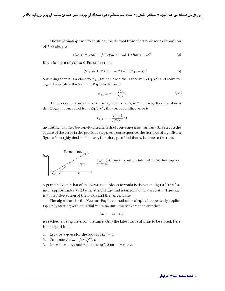
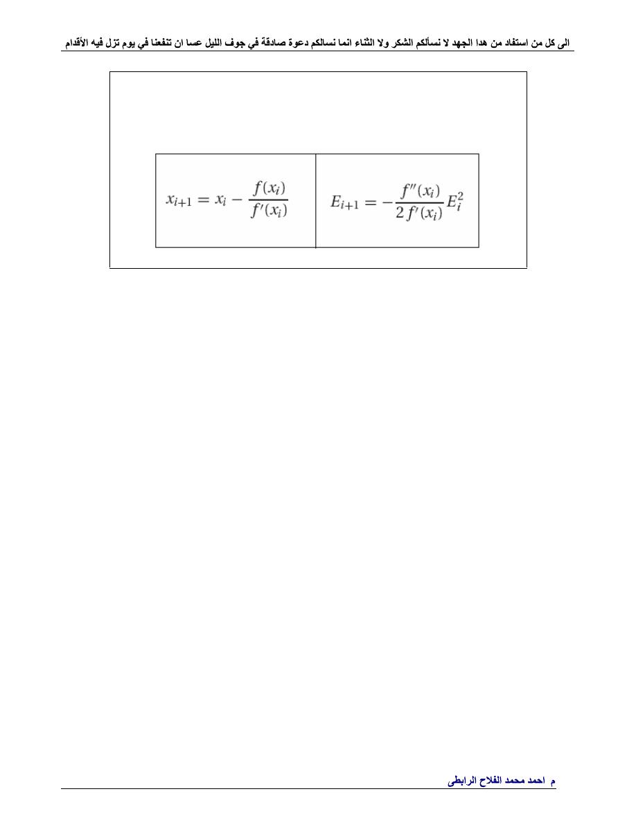
Newton
–
Raphson Method
.
Ahmad_engineer21@yahoo.com

.
Ahmad_engineer21@yahoo.com
Example
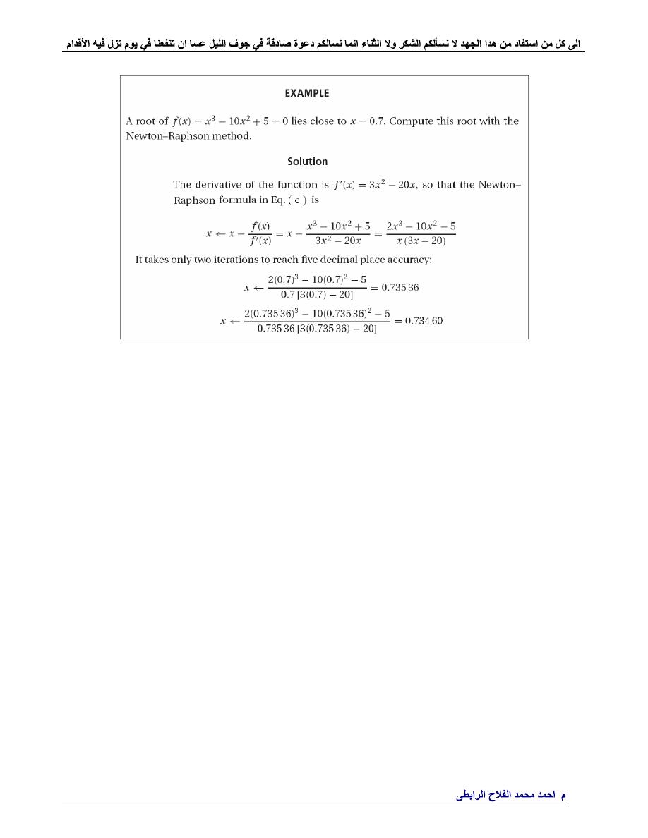
Use the Newton–Raphson Method to estimate the root of f(x)=e^(-x)-x,
employing an initial guess of x0=0
Solution
%------Newton–Raphson Method--------------------------
clc
x=[0];
tol=0.0000000007;
format
long
for
i=1:5;
fx=exp(-x(i))-x(i);
fxx=-exp(-x(i))-1 ;
fxxx=exp(-x(i));
x(i+1)=x(i)-(fx/fxx);
T.V(i)=(abs((x(i+1)-x(i))/x(i+1)))*100;
end
for
i=1:5;
e(i)=x(6)-x(i);
fxx=-exp(-x(6))-1 ;
fxxx=exp(-x(6));
e(i+1)=(-fxxx/2*fxx)*(e(i))^2;
end
if
abs(x(i+1)-x(i))<tol
disp(
' enough to here'
)
disp(
'------------'
)
disp(
' X(i+1) '
)
disp(
'-------------'
)
x'
disp(
'------------'
)
disp(
' T.V '
)
disp(
'-------------'
)
T.V'
disp(
'------------'
)
disp(
' E(i+1) '
)
disp(
'-------------'
)
e'
disp(
'-------------'
)
end
%-----------------------------------------------------

.
Ahmad_engineer21@yahoo.com
enough to here
-----------------------------
X(i+1)
-----------------------------
0
0.500000000000000
0.566311003197218
0.567143165034862
0.567143290409781
0.567143290409784
----------------------------
T.V
----------------------------
1.0e+002 *
1.000000000000000
0.117092909766624
0.001467287078375
0.000000221063919
0.000000000000005
----------------------------
E(i+1)
----------------------------
0.567143290409784
0.067143290409784
0.000832287212566
0.000000125374922
0.000000000000003
0.000000000000000
----------------------------
.
Ahmad_engineer21@yahoo.com
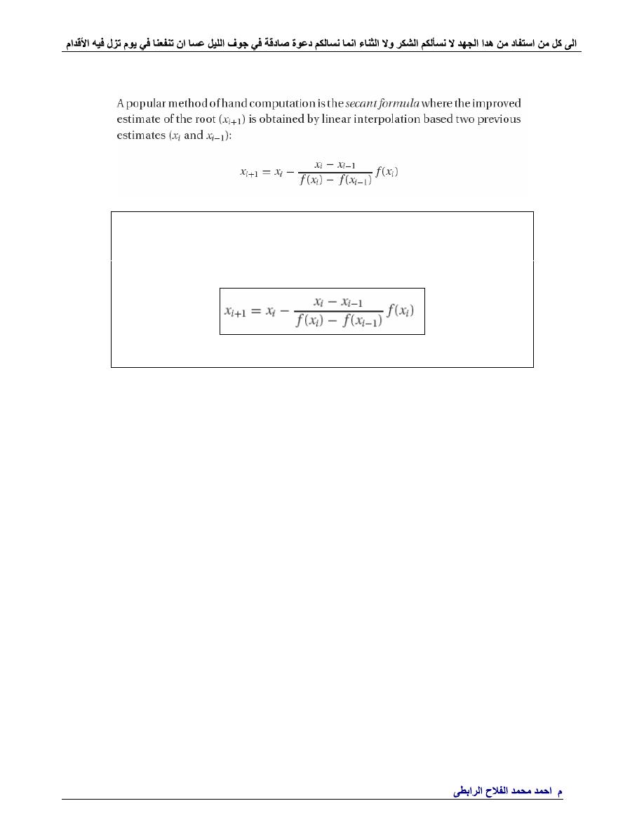
The secant Formula Method
Example
Use the The secant Formula Method to estimate the root of
f(x)=e^(-x)-x, employing an initial guess of x(i-1)=0 & x(0)=0
Solution
%------The secant Formula Method ------------------------
clc
x=[0 1];
TV=0.567143290409784;
format
long
for
i=2:6;
fx=exp(-x(i-1))-x(i-1);
fxx=exp(-x(i))-x(i);
x(i+1)=x(i)-((x(i)-x(i-1))*fxx)/(fxx-fx);
E_T(i)=(abs((TV-x(i+1))/TV))*100;
end
disp(
'------------'
)
disp(
' X(i+1) '
)
disp(
'-------------'
)
x'
disp(
'------------'
)
disp(
' E_T '
)
disp(
'-------------'
)
E_T'
disp(
'------------'
)
%-----------------------------------------------------

.
Ahmad_engineer21@yahoo.com
----------------------
X(i+1)
----------------------
0
1.000000000000000
0.612699836780282
0.563838389161074
0.567170358419745
0.567143306604963
0.567143290409705
---------------------
E_T
---------------------
0
8.032634281467328
0.582727734700312
0.004772693324310
0.000002855570996
0.000000000013997
--------------------
.
Ahmad_engineer21@yahoo.com
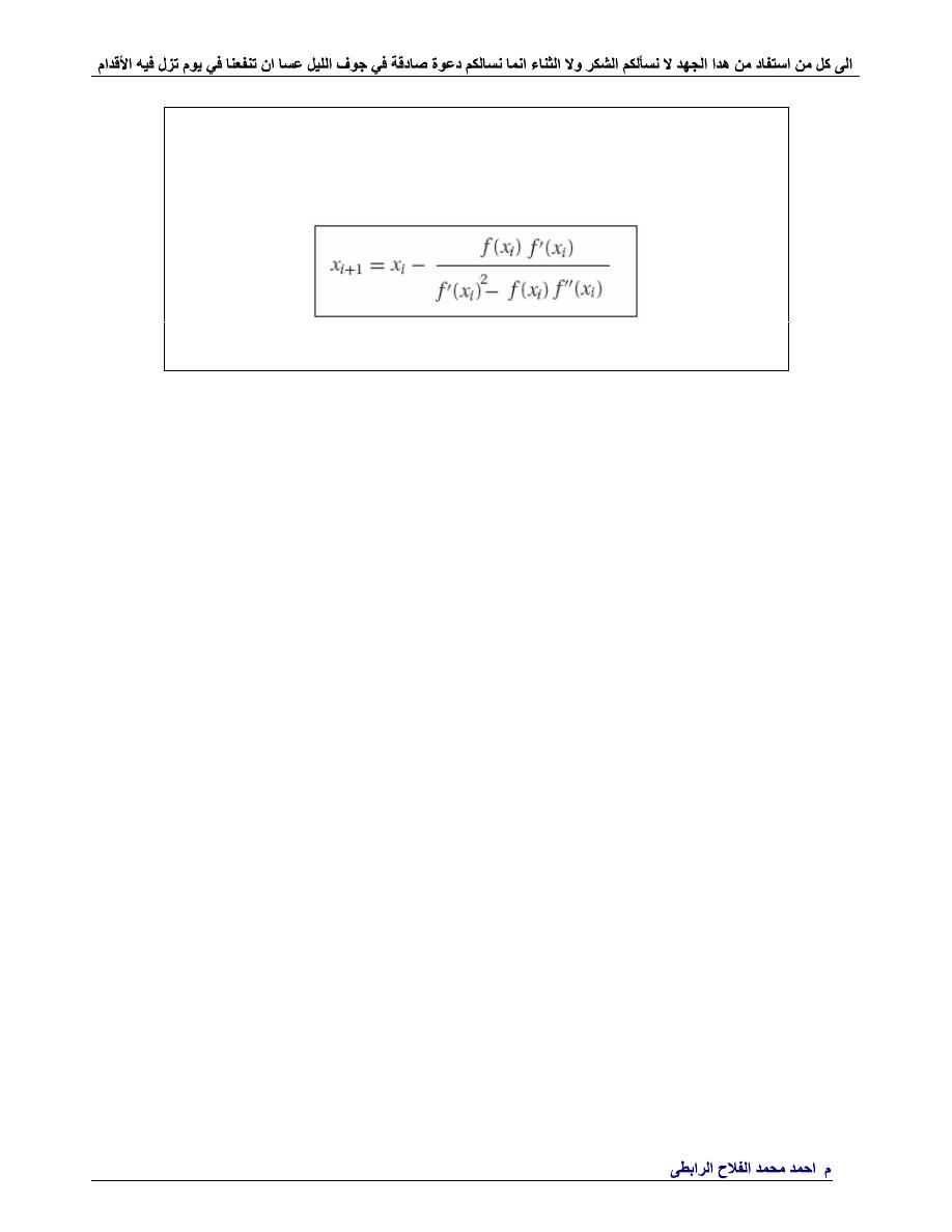
Example
Use N.R. Quadratically Method to estimate the multiple root of
f(x)=x^3-5x^2+7x-3, initial guess of x(0)=0
Solution
%------The N.R. Quadratically Method -----------------
clc
TV=1;
x=[0];
format
long
for
i=1:6;
fx=x(i)^3-5*x(i)^2+7*x(i)-3
fxx=3*x(i)^2-10*x(i)+7
fxxx=6*x(i)-10
x(i+1)=x(i)-(fx*fxx)/((fxx)^2-fx*fxxx);
E_T(i)=(abs((TV-x(i+1))/TV))*100;
end
disp(
'------------'
)
disp(
' X(i+1) '
)
disp(
'-------------'
)
x'
disp(
'------------'
)
disp(
' E_T '
)
disp(
'-------------'
)
E_T'
disp(
'------------'
)
%------------------------------------------------
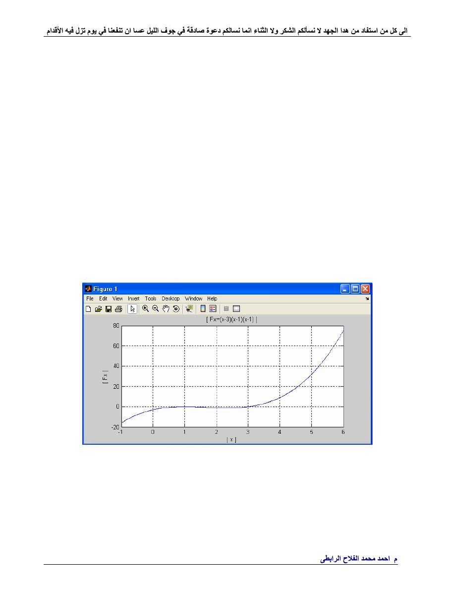
%------Multiple Roots---------
%--fx=(x-3)(x-1)(x-1)---------
clc
for
x=-1:0.01:6;
fx=x.^3-5.*x.^2+7.*x-3
plot(x,fx)
hold
on
end
grid
title(
'(x-3)(x-1)(x-1)'
)
xlabel(
'x'
)
ylabel(
'fx'
)
%----------------------------
.
Ahmad_engineer21@yahoo.com
---------------------------
X(i+1)
---------------------------
0
1.105263157894737
1.003081664098603
1.000002381493816
1.000000000037312
1.000000000074625
1.000000000074625
----------------------------
E_T
----------------------------
10.526315789473696
0.308166409860333
0.000238149381548
0.000000003731215
0.000000007462475
0.000000007462475
----------------------------
.
Ahmad_engineer21@yahoo.com
Example
Use the Newton–Raphson Method to estimate the root of
f(x)=x^3-5x^2+7x-3, initial guess of x(0)=4
Solution
%------Newton–Raphson Method--------------------------
clc
x=[4];
tol=0.0007;
TV=3;
format
long
for
i=1:5;
fx=x(i)^3-5*x(i)^2+7*x(i)-3;
fxx=3*x(i)^2-10*x(i)+7;
x(i+1)=x(i)-(fx/fxx);
E_T(i)=(abs((TV-x(i+1))/TV))*100;
end
for
i=1:5;
e(i)=x(6)-x(i);
fx=x(i)^3-5*x(i)^2+7*x(i)-3;
fxx=3*x(i)^2-10*x(i)+7;
fxxx=6*x(i)-10;
e(i+1)=(-fxxx/2*fxx)*(e(i))^2;
end
if
abs(TV-x(i+1))<tol
disp(
' enough to here'
)
disp(
'------------'
)
disp(
' X(i+1) '
)
disp(
'-------------'
)
x'
disp(
'------------'
)
disp(
' T.V '
)
disp(
'-------------'
)
E_T'
disp(
'------------'
)
disp(
' E(i+1) '
)
disp(
'-------------'
)
e'
disp(
'-------------'
)
end
%-----------------------------------------------------

.
Ahmad_engineer21@yahoo.com
enough to here
---------------------
X(i+1)
---------------------
4.000000000000000
3.400000000000000
3.100000000000000
3.008695652173913
3.000074640791192
3.000000005570623
---------------------
T.V
---------------------
13.333333333333330
3.333333333333322
0.289855072463781
0.002488026373060
0.000000185687436
0.000000007462475
--------------------
E(i+1)
--------------------
-0.999999994429377
-0.399999994429377
-0.099999994429377
-0.008695646603290
-0.000074635220569
-0.000000089144954
---------------------

.
Ahmad_engineer21@yahoo.com
Gauss Elimination Method
Example
Use the Gauss Elimination Method with MATLAB to solve the
following equations
2x1+x2-x3=5---------------------------(1)
X1+2x2+4x3=10-----------------------(2)
5x1+4x2-x3=14------------------------(3)
Solution:
%----- Gauss Elimination Method------------------------------
clc
A=[2 1 -1;1 2 4;5 4 -1];
b=[5 10 14];
if
size(b,2) > 1; b = b';
end
% b must be column vector
n = length(b);
for
k = 1:n-1
% Elimination phase
for
i= k+1:n
if
A(i,k) ~= 0
lambda = A(i,k)/A(k,k);
A(i,k+1:n) = A(i,k+1:n) - lambda*A(k,k+1:n);
b(i)= b(i) - lambda*b(k);
end
end
end
if
nargout == 2; det = prod(diag(A));
end
for
k = n:-1:1
% Back substitution phase
b(k) = (b(k) - A(k,k+1:n)*b(k+1:n))/A(k,k);
fprintf('
end
x = b
%----------------------------------------------------------
x =
4
-1
2

.
Ahmad_engineer21@yahoo.com
.
.
.
.
.
