
Don't forget to check out the Online Learning Center, www.mhhe.com/forouzan for
additional resources!
Instructors and students using Data Communications and Networking, Fourth Edition
by Behrouz A. Forouzan will find a wide variety of resources available at the Online
Learning Center, www.mhhe.comlforouzan
Instructor Resources
Instructors can access the following resources by contacting their McGraw-Hill Repre-
sentative for a secure password.
a
PowerPoint Slides. Contain figures, tables, highlighted points, and brief descriptions
of each section.
o
Complete Solutions Manual. Password-protected solutions to all end-of-chapter
problems are provided.
a
Pageout. A free tool that helps you create your own course website.
D
Instructor Message Board. Allows you to share ideas with other instructors
using the text.
Student Resources
The student resources are available to those students using the book. Once you have
accessed the Online Learning Center, click on
Resources," then select a chap-
ter from the drop down menu that appears. Each chapter has a wealth of materials to
help you review communications and networking concepts. Included are:
a
Chapter Summaries. Bulleted summary points provide an essential review of
major ideas and concepts covered in each chapter.
a
Student Solutions Manual. Contains answers for odd-numbered problems.
o
Glossary. Defines key terms presented in the book.
o
Flashcards. Facilitate learning through practice and review.
a
Animated Figures. Visual representations model key networking concepts, bringing
them to life.
D
Automated Quizzes. Easy-to-use quizzes strengthen learning and emphasize impor-
tant ideas from the book.
a
Web links. Connect students to additional resources available online.


DATA
COMMUNICATIONS
AND
NETWORKING

McGraw-Hill Forouzan Networking Series
Titles
by
Behrouz A. Forouzan:
Data Communications and Networking
TCPflP Protocol Suite
Local Area Networks
Business Data Communications

DATA
COMMUNICATIONS
AND
NETWORKING
Fourth Edition
Behrouz A. Forouzan
DeAnza College
with
Sophia Chung Fegan
Higher Education
Boston
Burr Ridge, IL
Dubuque, IA
Madison, WI
New York
San Francisco
S1. Louis
Bangkok
Bogota
Caracas
Kuala Lumpur
Lisbon
London
Madrid
Mexico City
Milan
Montreal
New Delhi
Santiago
Seoul
Singapore
Sydney
Taipei
Toronto

The
McGraw·HiII
Higher Education
DATA COMMUNICATIONS AND NETWORKING, FOURTH EDITION
Published by McGraw-Hill, a business unit of The McGraw-Hill Companies. Inc., 1221 Avenue
of the Americas, New York, NY 10020. Copyright © 2007 by The McGraw-Hill Companies, Inc.
AlI rights reserved. No part of this publication may be reproduced or distributed in any form or
by any means, or stored in a database or retrieval system, without the prior written consent of
The McGraw-Hill Companies, Inc., including, but not limited to, in any network or other
electronic storage or transmission, or broadcast for distance learning.
Some ancillaries, including electronic and print components, may not be available to customers
outside the United States.
This book is printed on acid-free paper.
1234567890DOC/DOC09876
ISBN-13
978-0-07-296775-3
ISBN-to
0-07-296775-7
Publisher: Alan R. Apt
Developmental Editor: Rebecca Olson
Executive Marketing Manager: Michael Weitz
Senior Project Manager: Sheila M. Frank
Senior Production Supervisor: Kara Kudronowicz
Senior Media Project Manager: Jodi K. Banowetz
Associate Media Producer: Christina Nelson
Senior Designer: David
Hash
Cover Designer: Rokusek Design
(USE) Cover Image: Women ascending Mount McKinley, Alaska. Mount McKinley (Denali)
12,000 feet, ©Allan Kearney/Getty Images
Compositor: Interactive Composition Corporation
Typeface: 10/12 Times Roman
Printer: R. R. Donnelley Crawfordsville, IN
Library of Congress
Data
Forouzan, Behrouz A.
Data communications and networking
I
Behrouz
A
Forouzan.
4th ed.
p. em.
(McGraw-HilI Forouzan networking series)
Includes index.
ISBN 978-0-07-296775-3 -
ISBN 0-07-296775-7 (hard eopy : alk. paper)
1. Data transmission systems. 2. Computer networks.
I.
Title. II. Series.
TK5105.F6617
004.6--dc22
www.mhhe.com
2007
2006000013
CIP

To
lny
wife, Faezeh, with love
Behrouz Forouzan


Preface
XXlX
PART 1
Overview
1
Chapter 1
Introduction
3
Chapter 2
Network Models
27
PART 2
Chapter 3
Chapter 4
Chapter 5
Chapter 6
Chapter 7
Chapter 8
Chapter 9
PART 3
Chapter 10
Chapter
11
Chapter 12
Chapter 13
Chapter 14
Chapter 15
Chapter 16
Chapter 17
Chapter 18
Physical Layer and Media
55
Data and Signals
57
Digital Transmission
101
Analog Transmission
141
Bandwidth Utilization: Multiplexing and Spreading
161
Transmission Media
191
Switching
213
Using Telephone and Cable Networksfor Data Transmission
241
Data Link Layer
265
Error Detection and Correction
267
Data Link Control
307
Multiple Access
363
Wired LANs: Ethernet
395
Wireless LANs
421
Connecting LANs, Backbone Networks, and Virtual LANs
445
Wireless WANs: Cellular Telephone and Satellite Networks
467
SONETISDH
491
Virtual-Circuit
Frame Relay andATM
517
vii
viii
BRIEF CONTENTS
PART 4
Chapter 19
Chapter 20
Chapter 21
Chapter 22
PARTS
Chapter 23
Chapter 24
PART 6
Chapter 25
Chapter 26
Chapter 27
Chapter 28
Chapter 29
Network Layer
547
Layer: Logical Addressing
549
Layer: Internet Protocol
579
Address Mapping, Error Reporting,
and Multicasting
611
Network Layer: Delivery, Fonvarding,
Routing
647
Transport Layer
701
Process-to-Process Delivery: UDp, TCP, and SCTP
703
Congestion Control and Quality
761
Application Layer
795
Domain Name
797
Remote Logging, Electronic Mail, and File
817
WWW and HTTP
Network Management: SNMP
873
Multimedia
901
PART 7
Security
929
Chapter 30
tog raphy
931
Chapter 31
Network
961
Chapter 32
Securit}' in the Internet: IPSec, SSLlTLS, PCp, VPN,
and Firewalls
Appendix A
Unicode
1029
Appendix B
Systems
1037
Appendix C
Mathematical Review
1043
Appendix D
8B/6T Code
1055
Appendix E
Telephone History
1059
Appendix F
Co!1tact Addresses
1061
Appendix G
RFCs
1063
Appendix H
UDP and TCP Ports
1065
1067
1071
References
1107
Index
IIII

Preface
xxix
PART 1
Overview
1
Chapter 1
Introduction
3
1.1
DATA COMMUNICATIONS
3
Components
4
Data Representation
5
DataFlow
6
1.2
NETWORKS
7
Distributed Processing
7
Network Criteria
7
Physical Structures
8
Network Models
13
Categories of Networks
13
Interconnection of Networks: Internetwork
IS
1.3
THE INTERNET
16
A Brief History
17
The Internet Today
17
1.4
PROTOCOLS AND STANDARDS
19
Protocols
19
Standards
19
Standards Organizations
20
Internet Standards
21
1.5
RECOMMENDED READING
21
Books
21
Sites
22
RFCs
22
1.6
KEY TERMS
22
1.7
SUMMARY
23
1.8
PRACTICE SET
24
Review Questions
24
Exercises
24
Research Activities
25
Chapter 2
Network Models
27
2.1
LAYERED TASKS
27
Sender, Receiver, and Carrier
28
Hierarchy
29
ix

x
CONTENTS
2.2
THE OSI MODEL
29
Layered Architecture
30
Peer-to-Peer Processes
30
Encapsulation
33
2.3
LAYERS IN THE OSI MODEL
33
Physical Layer
33
Data Link Layer
34
Network Layer
36
Transport Layer
37
Session Layer
39
Presentation Layer
39
Application Layer
41
Summary of Layers
42
2.4
TCP/IP
PROTOCOL SUITE
42
Physical and Data Link Layers
43
Network Layer
43
Transport Layer
44
Application Layer
45
2.5
ADDRESSING
45
Physical Addresses
46
Logical Addresses
47
Port Addresses
49
Specific Addresses
50
2.6
RECOMMENDED READING
50
Books
51
Sites
51
RFCs
51
2.7
KEY lERMS
51
2.8
SUMMARY
52
2.9
PRACTICE SET
52
Review Questions
52
Exercises
53
Research Activities
54
PART 2
Physical Layer and Media
55
Chapter 3
Data and Signals
57
3.1
ANALOG AND DIGITAL
57
Analog and Digital Data
57
Analog and Digital Signals
58
Periodic and Nonperiodic Signals
58
3.2
PERIODIC ANALOG SIGNALS
59
Sine Wave
59
Phase
63
Wavelength
64
Time and Frequency Domains
65
Composite Signals
66
Bandwidth
69
3.3
DIGITAL SIGNALS
71
Bit Rate
73
Bit Length
73
Digital Signal as a Composite Analog Signal
74
Transmission of Digital Signals
74

3.4
TRANSMISSION IMPAIRMENT
80
Attenuation
81
Distortion
83
Noise
84
3.5
DATA RATE LIMITS
85
Noiseless Channel: Nyquist Bit Rate
86
Noisy Channel: Shannon Capacity
87
Using Both Limits
88
3.6
PERFORMANCE
89
Bandwidth
89
Throughput
90
Latency (Delay)
90
Bandwidth-Delay Product
92
Jitter
94
3.7
RECOMMENDED READING
94
Books
94
3.8
KEYTERMS
94
3.9
SUMMARY
95
3.10
PRACTICE SET
96
Review Questions
96
Exercises
96
Chapter 4
Digital Transmission
101
4.1
DIGITAL-TO-DIGITAL CONVERSION
101
Line Coding
101
Line Coding Schemes
106
Block Coding
115
Scrambling
118
4.2
ANALOG-TO-DIGITAL CONVERSION
120
Pulse Code Modulation (PCM)
121
Delta Modulation (DM)
129
4.3
TRANSMISSION MODES
131
Parallel Transmission
131
Serial Transmission
132
4.4
RECOMMENDED READING
135
Books
135
4.5
KEYTERMS
135
4.6
SUMMARY
136
4.7
PRACTICE SET
137
Review Questions
137
Exercises
137
Chapter 5
Analog
141
5.1
DIGITAL-TO-ANALOG CONVERSION
141
Aspects of Digital-to-Analog Conversion
142
Amplitude Shift Keying
143
Frequency Shift Keying
146
Phase Shift Keying
148
Quadrature Amplitude Modulation
152
5.2
ANALOG-TO-ANALOG CONVERSION
152
Amplitude Modulation
153
Frequency Modulation
154
Phase Modulation
155
CONTENTS
xi

xii
CONTENTS
5.3
RECOMMENDED READING
156
Books
156
5.4
KEY lERMS
157
5.5
SUMMARY
157
5.6
PRACTICE SET
158
Review Questions
158
Exercises
158
Chapter 6
Multiplexing
and Spreading
161
6.1
MULTIPLEXING
161
Frequency-Division Multiplexing
162
Wavelength-Division Multiplexing
167
Synchronous Time-Division Multiplexing
169
Statistical Time-Division Multiplexing
179
6.2
SPREAD SPECTRUM
180
Frequency Hopping Spread Spectrum (FHSS)
181
Direct Sequence Spread Spectrum
184
6.3
RECOMMENDED READING
185
Books
185
6.4
KEY lERMS
185
6.5
SUMMARY
186
6.6
PRACTICE SET
187
Review Questions
187
Exercises
187
Chapter 7
Transmission Media
191
7.1
GUIDED MEDIA
192
Twisted-Pair Cable
193
Coaxial Cable
195
Fiber-Optic Cable
198
7.2
UNGUIDED MEDIA: WIRELESS
203
Radio Waves
205
Microwaves
206
Infrared
207
7.3
RECOMMENDED READING
208
Books
208
7.4
KEY lERMS
208
7.5
SUMMARY
209
7.6
PRACTICE SET
209
Review Questions
209
Exercises
210
Chapter 8
213
8.1
CIRCUIT-SWITCHED NETWORKS
214
Three Phases
217
Efficiency
217
Delay
217
Circuit-Switched Technology in Telephone Networks
218
8.2
DATAGRAM NETWORKS
218
Routing Table
220

CONTENTS
xiii
Efficiency
220
Delay
221
Datagram Networks in the Internet
221
8.3
VIRTUAL-CIRCUIT NETWORKS
221
Addressing
222
Three Phases
223
Efficiency
226
Delay in Virtual-Circuit Networks
226
Circuit-Switched Technology in WANs
227
8.4
STRUCTURE OF A SWITCH
227
Structure of Circuit Switches
227
Structure of Packet Switches
232
8.5
RECOMMENDED READING
235
Books
235
8.6
KEY TERMS
235
8.7
SUMMARY
236
8.8
PRACTICE SET
236
Review Questions
236
Exercises
237
Chapter 9
Using Telephone and Cable Networks for Data
Transm,ission
241
9.1
1ELEPHONE NETWORK
241
Major Components
241
LATAs
242
Signaling
244
Services Provided by Telephone Networks
247
9.2
DIAL-UP MODEMS
248
Modem Standards
249
9.3
DIGITAL SUBSCRIBER LINE
251
ADSL
252
ADSL Lite
254
HDSL
255
SDSL
255
VDSL
255
Summary
255
9.4
CABLE TV NETWORKS
256
Traditional Cable Networks
256
Hybrid Fiber-Coaxial (HFC) Network
256
9.5
CABLE TV FOR DATA TRANSFER
257
Bandwidth
257
Sharing
259
CM and CMTS
259
Data Transmission Schemes: DOCSIS
260
9.6
RECOMMENDED READING
261
Books
261
9.7
KEY TERMS
261
9.8
SUMMARY
262
9.9
PRACTICE SET
263
Review Questions
263
Exercises
264

xiv
CONTENTS
PART 3
Data Link Layer
265
Chapter 10
Error Detection and Correction
267
10.1
INTRODUCTION
267
Types of Errors
267
Redundancy
269
Detection Versus Correction
269
Forward Error Correction Versus Retransmission
269
Coding
269
Modular Arithmetic
270
10.2
BLOCK CODING
271
Error Detection
272
Error Correction
273
Hamming Distance
274
Minimum Hamming Distance
274
10.3
LINEAR BLOCK CODES
277
Minimum Distance for Linear Block Codes
278
Some Linear Block Codes
278
10.4
CYCLIC CODES
284
Cyclic Redundancy Check
284
Hardware Implementation
287
Polynomials
291
Cyclic Code Analysis
293
Advantages of Cyclic Codes
297
Other Cyclic Codes
297
10.5
CHECKSUM
298
Idea
298
One's Complement
298
Internet Checksum
299
10.6
RECOMMENDED READING
30 I
Books
301
RFCs
301
10.7
KEY lERMS
301
10.8
SUMMARY
302
10.9
PRACTICE SET
303
Review Questions
303
Exercises
303
Chapter 11
Data Link Control
307
11.1
FRAMING
307
Fixed-Size Framing
308
Variable-Size Framing
308
11.2
FLOW AND ERROR CONTROL
311
Flow Control
311
Error Control
311
11.3
PROTOCOLS
311
11.4
NOISELESS CHANNELS
312
Simplest Protocol
312
Stop-and-Wait Protocol
315
11.5
NOISY CHANNELS
318
Stop-and-Wait Automatic Repeat Request
318
Go-Back-N
Automatic Repeat Request
324

11.6
11.7
11.8
11.9
11.10
11.11
Selective Repeat Automatic Repeat Request
Piggybacking
339
HDLC
340
Configurations and Transfer Modes
340
Frames
341
Control Field
343
POINT-TO-POINT PROTOCOL
346
Framing
348
Transition Phases
349
Multiplexing
350
Multilink PPP
355
RECOMMENDED READING
357
Books
357
KEY TERMS
357
SUMMARY
358
PRACTICE SET
359
Review Questions
359
Exercises
359
332
CONTENTS
xv
Chapter 12
Multiple Access
363
12.1
RANDOMACCESS
364
ALOHA
365
Carrier Sense Multiple Access (CSMA)
370
Carrier Sense Multiple Access with Collision Detection
(CSMAlCD)
373
Carrier Sense Multiple Access with Collision Avoidance
(CSMAlCA)
377
12.2
CONTROLLED ACCESS
379
Reservation
379
Polling
380
Token Passing
381
12.3
CHANNELIZATION
383
Frequency-Division Multiple Access (FDMA)
383
Time-Division Multiple Access (TDMA)
384
Code-Division Multiple Access (CDMA)
385
12.4
RECOMMENDED READING
390
Books
391
12.5
KEY TERMS
391
12.6
SUMMARY
391
12.7
PRACTICE SET
392
Review Questions
392
Exercises
393
Research Activities
394
Chapter 13
Wired LANs: Ethernet
395
13.1
IEEE STANDARDS
395
Data Link Layer
396
Physical Layer
397
13.2
STANDARD ETHERNET
397
MAC Sublayer
398
Physical Layer
402
13.3
CHANGES IN THE STANDARD
406
Bridged Ethernet
406
Switched Ethernet
407
Full-Duplex Ethernet
408

xvi
CONTENTS
13.4
FAST ETHERNET
409
MAC Sublayer
409
Physical Layer
410
13.5
GIGABIT ETHERNET
412
MAC Sublayer
412
Physical Layer
414
Ten-Gigabit Ethernet
416
13.6
RECOMMENDED READING
417
Books
417
13.7
KEY TERMS
417
13.8
SUMMARY
417
13.9
PRACTICE SET
418
Review Questions
418
Exercises
419
Chapter 14
Wireless LANs
421
14.1
IEEE 802.11
421
Architecture
421
MAC Sublayer
423
Addressing Mechanism
428
Physical Layer
432
14.2
BLUETOOTH
434
Architecture
435
Bluetooth Layers
436
Radio Layer
436
Baseband Layer
437
L2CAP
440
Other Upper Layers
441
14.3
RECOMMENDED READING
44 I
Books
442
14.4
KEYTERMS
442
14.5
SUMMARY
442
14.6
PRACTICE SET
443
Review Questions
443
Exercises
443
Chapter 15
Connecting LANs, Backbone Networks,
and VirtuaL LANs
445
15.1
CONNECTING DEVICES
445
Passive Hubs
446
Repeaters
446
Active Hubs
447
Bridges
447
Two-Layer Switches
454
Routers
455
Three-Layer Switches
455
Gateway
455
15.2
BACKBONE NETWORKS
456
Bus Backbone
456
Star Backbone
457
Connecting Remote LANs
457

15.3
VIRTUAL LANs
458
Membership
461
Configuration
461
Communication Between Switches
462
IEEE Standard
462
Advantages
463
15.4
RECOMMENDED READING
463
Books
463
Site
463
15.5
KEY TERMS
463
15.6
SUMMARY
464
15.7
PRACTICE SET
464
Review Questions
464
Exercises
465
CONTENTS
xvii
Chapter 16
Wireless WANs: Cellular Telephone and
Satellite Networks
467
16.1
CELLULAR TELEPHONY
467
Frequency-Reuse Principle
467
Transmitting
468
Receiving
469
Roaming
469
First Generation
469
Second Generation
470
Third Generation
477
16.2
SATELLITE NETWORKS
478
Orbits
479
Footprint
480
Three Categories of Satellites
480
GEO Satellites
481
MEO Satellites
481
LEO Satellites
484
16.3
RECOMMENDED READING
487
Books
487
16.4
KEY TERMS
487
16.5
SUMMARY
487
16.6
PRACTICE SET
488
Review Questions
488
Exercises
488
Chapter 17
SONETISDH
491
17.1
ARCHITECTURE
491
Signals
491
SONET Devices
492
Connections
493
17.2
SONET LAYERS
494
Path Layer
494
Line Layer
495
Section Layer
495
Photonic Layer
495
Device-Layer Relationships
495

xviii
CONTENTS
17.3
SONET FRAMES
496
Frame, Byte, and Bit Transmission
496
STS-l Frame Format
497
Overhead Summary
501
Encapsulation
501
17.4
STS MULTIPLEXING
503
Byte Interleaving
504
Concatenated Signal
505
AddlDrop Multiplexer
506
17.5
SONET NETWORKS
507
Linear Networks
507
Ring Networks
509
Mesh Networks
510
17.6
VIRTUAL TRIBUTARIES
512
Types ofVTs
512
17.7
RECOMMENDED READING
513
Books
513
17.8
KEY lERMS
513
17.9
SUMMARY
514
17.1 0 PRACTICE SET
514
Review Questions
514
Exercises
515
Chapter 18
Virtual-Circuit Networks:
Frame
and ATM
517
18.1
FRAME RELAY
517
Architecture
518
Frame Relay Layers
519
Extended Address
521
FRADs
522
VOFR
522
LMI
522
Congestion Control and Quality of Service
522
18.2
ATM
523
Design Goals
523
Problems
523
Architecture
526
Switching
529
ATM Layers
529
Congestion Control and Quality of Service
535
18.3
ATM LANs
536
ATM LAN Architecture
536
LAN Emulation (LANE)
538
Client/Server Model
539
Mixed Architecture with Client/Server
540
18.4
RECOMMENDED READING
540
Books
541
18.5
KEY lERMS
541
18.6
SUMMARY
541
18.7
PRACTICE SET
543
Review Questions
543
Exercises
543

CONTENTS
xix
PART 4
Network Layer
547
Chapter 19
Netvl/ark Layer: Logical Addressing
549
19.1
IPv4ADDRESSES
549
Address Space
550
Notations
550
Classful Addressing
552
Classless Addressing
555
Network Address Translation (NAT)
563
19.2
IPv6 ADDRESSES
566
Structure
567
Address Space
568
19.3
RECOMMENDED READING
572
Books
572
Sites
572
RFCs
572
19.4
KEY TERMS
572
19.5
SUMMARY
573
19.6
PRACTICE SET
574
Review Questions
574
Exercises
574
Research Activities
577
Chapter 20
Network Layer: Internet Protocol
579
20.1
INTERNETWORKING
579
Need for Network Layer
579
Internet as a Datagram Network
581
Internet as a Connectionless Network
582
20.2
IPv4
582
Datagram
583
Fragmentation
589
Checksum
594
Options
594
20.3
IPv6
596
Advantages
597
Packet Format
597
Extension Headers
602
20.4
TRANSITION FROM IPv4 TO IPv6
603
Dual Stack
604
Tunneling
604
Header Translation
605
20.5
RECOMMENDED READING
605
Books
606
Sites
606
RFCs
606
20.6
KEY TERMS
606
20.7
SUMMARY
607
20.8
PRACTICE SET
607
Review Questions
607
Exercises
608
Research Activities
609

xx
CONTENTS
Chapter 21
Network Layer: Address Mapping, Error Reporting,
and Multicasting
611
21.1
ADDRESS MAPPING
611
Mapping Logical to Physical Address: ARP
612
Mapping Physical to Logical Address: RARp, BOOTP, and DHCP
618
21.2
ICMP
621
Types of Messages
621
Message Format
621
Error Reporting
622
Query
625
Debugging Tools
627
21.3
IGMP
630
Group Management
630
IGMP Messages
631
Message Format
631
IGMP Operation
632
Encapsulation
635
Netstat Utility
637
21.4
ICMPv6
638
Error Reporting
638
Query
639
21.5
RECOMMENDED READING
640
Books
641
Site
641
RFCs
641
21.6
KEYTERMS
641
21.7
SUMMARY
642
21.8
PRACTICE SET
643
Review Questions
643
Exercises
644
Research Activities
645
Chapter 22
Network Layer: Delivery, Forwarding,
and Routing
647
22.1
DELIVERY
647
Direct Versus Indirect Delivery
647
22.2
FORWARDING
648
Forwarding Techniques
648
Forwarding Process
650
Routing Table
655
22.3
UNICAST ROUTING PROTOCOLS
658
Optimization
658
Intra- and Interdomain Routing
659
Distance Vector Routing
660
Link State Routing
666
Path Vector Routing
674
22.4
MULTICAST ROUTING PROTOCOLS
678
Unicast, Multicast, and Broadcast
678
Applications
681
Multicast Routing
682
Routing Protocols
684

CONTENTS
xxi
22.5
RECOMMENDED READING
694
Books
694
Sites
694
RFCs
694
22.6
KEY lERMS
694
22.7
SUMMARY
695
22.8
PRACTICE SET
697
Review Questions
697
Exercises
697
Research Activities
699
PART 5
Transport Layer
701
Chapter 23
Process-fa-Process Delivery: UDp, TCp,
and
SeTP
703
23.1
PROCESS-TO-PROCESS DELIVERY
703
Client/Server Paradigm
704
Multiplexing and Demultiplexing
707
Connectionless Versus Connection-Oriented Service
707
Reliable Versus Unreliable
708
Three Protocols
708
23.2
USER DATAGRAM PROTOCOL (UDP)
709
Well-Known Ports for UDP
709
User Datagram
710
Checksum
711
UDP Operation
713
Use ofUDP
715
23.3
TCP
715
TCP Services
715
TCP Features
719
Segment
721
A TCP Connection
723
Flow Control
728
Error Control
731
Congestion Control
735
SCTP
736
SCTP Services
736
SCTP Features
738
Packet Format
742
An SCTP Association
743
Flow Control
748
Error Control
751
Congestion Control
753
23.5
RECOMMENDED READING
753
Books
753
Sites
753
RFCs
753
23.6
KEY lERMS
754
23.7
SUMMARY
754
23.8
PRACTICE SET
756
Review Questions
756
Exercises
757
Research Activities
759

xxii
CONTENTS
Chapter 24
Congestion Control and Quality
767
24.1
DATA lRAFFIC
761
Traffic Descriptor
76]
Traffic Profiles
762
24.2
CONGESTION
763
Network Performance
764
24.3
CONGESTION CONTROL
765
Open-Loop Congestion Control
766
Closed-Loop Congestion Control
767
24.4
lWO EXAMPLES
768
Congestion Control in TCP
769
Congestion Control in Frame Relay
773
24.5
QUALITY OF SERVICE
775
Flow Characteristics
775
Flow Classes
776
24.6
TECHNIQUES TO IMPROVE QoS
776
Scheduling
776
Traffic Shaping
777
Resource Reservation
780
Admission Control
780
24.7
INTEGRATED SERVICES
780
Signaling
781
Flow Specification
781
Admission
781
Service Classes
781
RSVP
782
Problems with Integrated Services
784
24.8
DIFFERENTIATED SERVICES
785
DS Field
785
24.9
QoS IN SWITCHED NETWORKS
786
QoS in Frame Relay
787
QoS inATM
789
24.10 RECOMMENDED READING
790
Books
791
24.11 KEY TERMS
791
24.12 SUMMARY
791
24.13 PRACTICE SET
792
Review Questions
792
Exercises
793
PART 6
Application Layer
795
Chapter 25
DO/nain Name Svstem
797
25.1
NAME SPACE
798
Flat Name Space
798
Hierarchical Name Space
798
25.2
DOMAIN NAME SPACE
799
Label
799
Domain Narne
799
Domain
801

25.3
25.4
25.5
25.6
25.7
25.8
25.9
25.10
25.11
25.12
25.13
25.14
DISTRIBUTION OF NAME SPACE
801
Hierarchy of Name Servers
802
Zone
802
Root Server
803
Primary and Secondary Servers
803
DNS IN THE INTERNET
803
Generic Domains
804
Country Domains
805
Inverse Domain
805
RESOLUTION
806
Resolver
806
Mapping Names to Addresses
807
Mapping Address to Names
807
Recursive Resolution
808
Iterative Resolution
808
Caching
808
DNS MESSAGES
809
Header
809
TYPES OF RECORDS
811
Question Record
811
Resource Record
811
REGISTRARS
811
DYNAMIC DOMAIN NAME SYSTEM (DDNS)
ENCAPSULATION
812
RECOMMENDED READING
812
Books
813
Sites
813
RFCs
813
KEY TERMS
813
SUMMARY
813
PRACTICE SET
814
Review Questions
814
Exercises
815
812
CONTENTS
xxiii
Chapter 26
Remote Logging, Electronic Mail, and File Transfer
817
26.1
REMOTE LOGGING
817
TELNET
817
26.2
ELECTRONIC MAIL
824
Architecture
824
User Agent
828
Message Transfer Agent: SMTP
834
Message Access Agent: POP and IMAP
837
Web-Based Mail
839
26.3
FILE TRANSFER
840
File Transfer Protocol (FTP)
840
Anonymous FTP
844
26.4
RECOMMENDED READING
845
Books
845
Sites
845
RFCs
845
26.5
KEY lERMS
845
26.6
SUMMARY
846

xxiv
CONTENTS
26.7
PRACTICE SET
847
Review Questions
847
Exercises
848
Research Activities
848
Chapter 27
WWW and HTTP
851
27.1
ARCHITECTURE
851
Client (Browser)
852
Server
852
Uniform Resource Locator
853
Cookies
853
27.2
WEB DOCUMENTS
854
Static Documents
855
Dynamic Documents
857
Active Documents
860
27.3
HTTP
861
HTTP Transaction
861
Persistent Versus Nonpersistent Connection
868
Proxy Server
868
27.4
RECOMMENDED READING
869
Books
869
Sites
869
RFCs
869
27.5
KEY 1ERMS
869
27.6
SUMMARY
870
27.7
PRACTICE SET
871
Review Questions
871
Exercises
871
Chapter 28
Network Management: SNMP
873
28.1
NETWORK MANAGEMENT SYSTEM
873
Configuration Management
874
Fault Management
875
Performance Management
876
Security Management
876
Accounting Management
877
28.2
SIMPLE NETWORK MANAGEMENT PROTOCOL (SNMP)
877
Concept
877
Management Components
878
Structure of Management Information
881
Management Information Base (MIB)
886
Lexicographic Ordering
889
SNMP
891
Messages
893
UDP Ports
895
Security
897
28.3
RECOMMENDED READING
897
Books
897
Sites
897
RFCs
897
28.4
KEY 1ERMS
897
28.5
SUMMARY
898

28.6
PRACTICE SET
899
Review Questions
899
Exercises
899
Chapter 29
Multimedia
901
29.1
DIGITIZING AUDIO AND VIDEO
902
Digitizing Audio
902
Digitizing Video
902
29.2
AUDIO AND VIDEO COMPRESSION
903
Audio Compression
903
Video Compression
904
29.3
STREAMING STORED AUDIO/VIDEO
908
First Approach: Using a Web Server
909
Second Approach: Using a Web Server with Metafile
909
Third Approach: Using a Media Server
910
Fourth Approach: Using a Media Server and RTSP
911
29.4
STREAMING LIVE AUDIOIVIDEO
912
29.5
REAL-TIME INTERACTIVE AUDIOIVIDEO
912
Characteristics
912
29.6
RTP
916
RTP Packet Format
917
UDPPort
919
29.7
RTCP
919
Sender Report
919
Receiver Report
920
Source Description Message
920
Bye Message
920
Application-Specific Message
920
UDP Port
920
29.8
VOICE OVER IP
920
SIP
920
H.323
923
29.9
RECOMMENDED READING
925
Books
925
Sites
925
29.10 KEY 1ERMS
925
29.11 SUMMARY
926
29.12 PRACTICE SET
927
Review Questions
927
Exercises
927
Research Activities
928
PART 7
Security
929
Chapter 30
Cryptography
931
30.1
INTRODUCTION
931
Definitions
931
Categories
932
30.2
SYMMETRIC-KEY CRYPTOGRAPHY
935
Traditional Ciphers
935
Simple Modem Ciphers
938
CONTENTS
xxv

xxvi
CONTENTS
Modern Round Ciphers
940
Mode of Operation
945
30.3
ASYMMETRIC-KEY CRYPTOGRAPHY
949
RSA
949
Diffie-Hellman
952
30.4
RECOMMENDED READING
956
Books
956
30.5
KEY TERMS
956
30.6
SUMMARY
957
30.7
PRACTICE SET
958
Review Questions
958
Exercises
959
Research Activities
960
Chapter 31
Network Security
961
31.1
SECURITY SERVICES
961
Message Confidentiality
962
Message Integrity
962
Message Authentication
962
Message Nonrepudiation
962
Entity Authentication
962
31.2
MESSAGE CONFIDENTIALITY
962
Confidentiality with Symmetric-Key Cryptography
963
Confidentiality with Asymmetric-Key Cryptography
963
31.3
MESSAGE INTEGRITY
964
Document and Fingerprint
965
Message and Message Digest
965
Difference
965
Creating and Checking the Digest
966
Hash Function Criteria
966
Hash Algorithms: SHA-1
967
31.4
MESSAGE AUTHENTICATION
969
MAC
969
31.5
DIGITAL SIGNATURE
971
Comparison
97
I
Need for Keys
972
Process
973
Services
974
Signature Schemes
976
31.6
ENTITY AUTHENTICATION
976
Passwords
976
Challenge-Response
978
31.7
KEY MANAGEMENT
981
Symmetric-Key Distribution
981
Public-Key Distribution
986
31.8
RECOMMENDED READING
990
Books
990
31.9
KEY TERMS
990
31.10 SUMMARY
991
31.11 PRACTICE SET
992
Review Questions
992
Exercises
993
Research Activities
994

CONTENTS
xxvii
Chapter 32
Security
the Internet: IPSec, SSUFLS, PGP, VPN,
and Firewalls
995
32.1
IPSecurity (lPSec)
996
Two Modes
996
Two Security Protocols
998
Security Association
1002
Internet Key Exchange (IKE)
1004
Virtual Private Network
1004
32.2
SSLffLS
1008
SSL Services
1008
Security Parameters
1009
Sessions and Connections
1011
Four Protocols
10 12
Transport Layer Security
1013
32.3
PGP
1014
Security Parameters
1015
Services
1015
A Scenario
1016
PGP Algorithms
1017
Key Rings
1018
PGP Certificates
1019
32.4
FIREWALLS
1021
Packet-Filter Firewall
1022
Proxy Firewall
1023
32.5
RECOMMENDED READING
1024
Books
1024
32.6
KEY lERMS
1024
32.7
SUMMARY
1025
32.8
PRACTICE SET
1026
Review Questions
1026
Exercises
1026
Appendix A
Unicode
1029
A.l
UNICODE
1029
Planes
1030
Basic Multilingual Plane (BMP)
1030
Supplementary Multilingual Plane (SMP)
1032
Supplementary Ideographic Plane (SIP)
1032
Supplementary Special Plane (SSP)
1032
Private Use Planes (PUPs)
1032
A.2
ASCII
1032
Some Properties of ASCII
1036
Appendix B
Numbering Systems
1037
B.l
BASE 10: DECIMAL
1037
Weights
1038
B.2
BASE 2: BINARY
1038
Weights
1038
Conversion
1038

xxviii
CONTENTS
B.3
BASE 16: HEXADECIMAL
1039
Weights
1039
Conversion
1039
A Comparison
1040
BA
BASE 256: IP ADDRESSES
1040
Weights
1040
Conversion
1040
B.5
OTHER CONVERSIONS
1041
Binary and Hexadecimal
1041
Base 256 and Binary
1042
Appendix C
Mathenwtical
1043
C.1
TRIGONOMETRIC FUNCTIONS
1043
Sine Wave
1043
Cosine Wave
1045
Other Trigonometric Functions
1046
Trigonometric Identities
1046
C.2
FOURIER ANALYSIS
1046
Fourier Series
1046
Fourier Transform
1048
C.3
EXPONENT AND LOGARITHM
1050
Exponential Function
1050
Logarithmic Function
1051
Appendix 0
8B/6T Code
1055
Appendix E
Telephone History
1059
Before 1984
1059
Between 1984 and 1996
1059
After 1996
1059
Appendix F
Contact Addresses
1061
Appendix G
RFCs
1063
Appendix H
UDP and TCP Ports
1065
Acronyms
1067
Glossary
1071
References
1107
Index
1111

Data communications and networking may be the fastest growing technologies in our
culture today. One of the ramifications of that growth is a dramatic increase in the number
of professions where an understanding of these technologies is essential for success-
and a proportionate increase in the number and types of students taking courses to learn
about them.
Features of the Book
Several features of this text are designed to make it particularly easy for students to
understand data communications and networking.
Structure
We have used the five-layer Internet model as the framework for the text not only because
a thorough understanding of the model is essential to understanding most current network-
ing theory but also because it is based on a structure of interdependencies: Each layer
builds upon the layer beneath it and supports the layer above it. In the same way, each con-
cept introduced in our text builds upon the concepts examined in the previous sections. The
Internet model was chosen because it is a protocol that is fully implemented.
This text is designed for students with little or no background in telecommunica-
tions or data communications. For this reason, we use a bottom-up approach. With this
approach, students learn first about data communications (lower layers) before learning
about networking (upper layers).
Visual Approach
The book presents highly technical subject matter without complex formulas by using a
balance of text and figures. More than 700 figures accompanying the text provide a
visual and intuitive opportunity for understanding the material. Figures are particularly
important in explaining networking concepts, which are based on connections and
transmission. Both of these ideas are easy to grasp visually.
Highlighted Points
We emphasize important concepts in highlighted boxes for quick reference and imme-
diate attention.
xxix

xxx
PREFACE
Examples and Applications
When appropriate, we have selected examples to reflect true-to-life situations. For exam-
ple, in Chapter 6 we have shown several cases of telecommunications in current telephone
networks.
Recommended Reading
Each chapter includes a list of books and sites that can be used for further reading.
Key Terms
Each chapter includes a list of key terms for the student.
Summary
Each chapter ends with a summary of the material covered in that chapter. The sum-
mary provides a brief overview of all the important points in the chapter.
Practice Set
Each chapter includes a practice set designed to reinforce and apply salient concepts.
It
consists of three parts: review questions, exercises, and research activities (only for
appropriate chapters). Review questions are intended to test the student's first-level under-
standing of the material presented in the chapter. Exercises require deeper understanding
of the materiaL Research activities are designed to create motivation for further study.
Appendixes
The appendixes are intended to provide quick reference material or a review of materi-
als needed to understand the concepts discussed in the book.
Glossary and Acronyms
The book contains an extensive glossary and a list of acronyms.
Changes in the Fourth Edition
The Fourth Edition has major changes from the Third Edition, both in the organization
and in the contents.
Organization
The following lists the changes in the organization of the book:
1. Chapter 6 now contains multiplexing as well as spreading.
2. Chapter 8 is now totally devoted to switching.
3. The contents of Chapter 12 are moved to Chapter 11.
4. Chapter 17 covers SONET technology.
5. Chapter 19 discusses IP addressing.
6. Chapter 20 is devoted to the Internet Protocol.
7. Chapter 21 discusses three protocols: ARP, ICMP, and IGMP.
8. Chapter 28 is new and devoted to network management in the Internet.
9. The previous Chapters 29 to 31 are now Chapters 30 to 32.

PREFACE
xxxi
Contents
We have revised the contents of many chapters including the following:
1. The contents of Chapters 1 to 5 are revised and augmented. Examples are added to
clarify the contents.
2. The contents of Chapter 10 are revised and augmented to include methods of error
detection and correction.
3. Chapter 11 is revised to include a full discussion of several control link protocols.
4. Delivery, forwarding, and routing of datagrams are added to Chapter 22.
5. The new transport protocol, SCTP, is added to Chapter 23.
6. The contents of Chapters 30, 31, and 32 are revised and augmented to include
additional discussion about security issues and the Internet.
7. New examples are added to clarify the understanding of concepts.
End Materials
1. A section is added to the end of each chapter listing additional sources for study.
2. The review questions are changed and updated.
3. The multiple-choice questions are moved to the book site to allow students to self-test
their knowledge about the contents of the chapter and receive immediate feedback.
4. Exercises are revised and new ones are added to the appropriate chapters.
5. Some chapters contain research activities.
Instructional Materials
Instructional materials for both the student and the teacher are revised and augmented.
The solutions to exercises contain both the explanation and answer including full col-
ored figures or tables when needed. The Powerpoint presentations are more compre-
hensive and include text and figures.
Contents
The book is divided into seven parts. The first part is an overview; the last part concerns
network security. The middle five parts are designed to represent the five layers of the
Internet model. The following summarizes the contents of each part.
Part One: Overview
The first part gives a general overview of data communications and networking. Chap-
ter 1 covers introductory concepts needed for the rest of the book. Chapter 2 introduces
the Internet model.
Part Two: Physical Layer
The second part is a discussion of the physical layer of the Internet model. Chapters 3
to 6 discuss telecommunication aspects of the physical layer. Chapter 7 introduces the
transmission media, which, although not part of the physical layer, is controlled by it.
Chapter 8 is devoted to switching, which can be used in several layers. Chapter 9 shows
how two public networks, telephone and cable TV, can be used for data transfer.

xxxii
PREFACE
Part Three: Data Link Layer
The third part is devoted to the discussion of the data link layer of the Internet model.
Chapter 10 covers error detection and correction. Chapters 11, 12 discuss issues related
to data link control. Chapters 13 through 16 deal with LANs. Chapters 17 and] 8 are
about WANs. LANs and WANs are examples of networks operating in the first two lay-
ers of the Internet model.
Part Four: Network Layer
The fourth part is devoted to the discussion of the network layer of the Internet model.
Chapter 19 covers IP addresses. Chapters 20 and 21 are devoted to the network layer
protocols such as IP, ARP, ICMP, and IGMP. Chapter 22 discusses delivery, forwarding,
and routing of packets in the Internet.
Part Five: Transport Layer
The fifth part is devoted to the discussion of the transport layer of the Internet model.
Chapter 23 gives an overview of the transport layer and discusses the services and
duties of this layer.
It
also introduces three transport-layer protocols: UDP, TCP, and
SCTP. Chapter 24 discusses congestion control and quality of service, two issues
related to the transport layer and the previous two layers.
Part Six: Application Layer
The sixth part is devoted to the discussion of the application layer of the Internet model.
Chapter 25 is about DNS, the application program that is used by other application pro-
grams to map application layer addresses to network layer addresses. Chapter 26 to 29
discuss some common applications protocols in the Internet.
Part Seven: Security
The seventh part is a discussion of security.
It
serves as a prelude to further study in this
subject. Chapter 30 briefly discusses cryptography. Chapter 31 introduces security
aspects. Chapter 32 shows how different security aspects can be applied to three layers
of the Internet model.
Online Learning Center
The McGraw-Hill Online Learning Center contains much additional material. Avail-
able at www.mhhe.com/forouzan. As students read through
Data Communications and
Networking,
they can go online to take self-grading quizzes. They can also access lec-
ture materials such as PowerPoint slides, and get additional review from animated fig-
ures from the book. Selected solutions are also available over the Web. The solutions to
odd-numbered problems are provided to students, and instructors can use a password to
access the complete set of solutions.
Additionally, McGraw-Hill makes it easy to create a website for your networking
course with an exclusive McGraw-Hill product called PageOut.
It
requires no prior
knowledge of HTML, no long hours, and no design skills on your part. Instead,
Out offers a series of templates. Simply fill them with your course information

PREFACE
xxxiii
click on one of 16 designs. The process takes under
an
hour and leaves you with a pro-
fessionally designed website.
Although PageOut offers "instant" development, the finished website provides pow-
erful features. An interactive course syllabus allows you to post content to coincide with
your lectures, so when students visit your PageOut website, your syllabus will direct them
to components of Forouzan's Online Learning Center, or specific material of your own.
How to Use the Book
This book is written for both an academic and a professional audience. The book can be
used as a self-study guide for interested professionals. As a textbook, it can be used for
a one-semester or one-quarter course. The following are some guidelines.
o
Parts one to three are strongly recommended.
o
four to six can be covered if there is no following course in
TCP/IP
protocol.
o
Part seven is recommended if there is no following course in network security.
Acknowledgments
It
is obvious that the development of a book of this scope needs the support of many people.
Peer Review
The most important contribution to the development of a book such as this comes from
peer reviews. We cannot express our gratitude in words to the many reviewers who
spent numerous hours reading the manuscript and providing us with helpful comments
and ideas. We would especially like to acknowledge the contributions of the following
reviewers for the third and fourth editions of this book.
Farid Ahmed, Catholic University
Kaveh Ashenayi, University of Tulsa
Yoris Au, University ofTexas, San Antonio
Essie Bakhtiar, Clayton College
&
State University
Anthony Barnard, University ofAlabama, Brimingham
A.T. Burrell, Oklahoma State University
Scott Campbell, Miami University
Teresa Carrigan, Blackburn College
Hwa Chang, Tufts University
Edward Chlebus, Illinois Institute ofTechnology
Peter Cooper, Sam Houston State University
Richard Coppins, Virginia Commonwealth University
Harpal Dhillon, Southwestern Oklahoma State University
Hans-Peter Dommel, Santa Clara University
M. Barry Dumas, Baruch College, CUNY
William Figg, Dakota State University
Dale Fox, Quinnipiac University
Terrence Fries, Coastal Carolina University
Errin Fulp, Wake Forest University

xxxiv
PREFACE
Sandeep Gupta,
Arizona State University
George Hamer,
South Dakota State University
James Henson,
California State University, Fresno
Tom Hilton,
Utah State University
Allen Holliday,
California State University, Fullerton
Seyed Hossein Hosseini,
University of Wisconsin, Milwaukee
Gerald Isaacs,
Carroll College, Waukesha
Hrishikesh Joshi,
DeVry University
E.S. Khosravi,
Southern University
Bob Kinicki,
Worcester Polytechnic University
Kevin Kwiat,
Hamilton College
Ten-Hwang Lai,
Ohio State University
Chung-Wei Lee,
Auburn University
Ka-Cheong Leung,
Texas Tech University
Gertrude Levine,
Fairleigh Dickinson University
Alvin Sek See Lim,
Auburn University
Charles Liu,
California State University, Los Angeles
Wenhang Liu,
California State University, Los Angeles
Mark Llewellyn,
University of Central Florida
Sanchita Mal-Sarkar,
Cleveland State University
Louis Marseille,
Harford Community College
Kevin McNeill,
University ofArizona
Arnold C. Meltzer,
George Washington University
Rayman Meservy,
Brigham Young University
Prasant Mohapatra,
University of California, Davis
Hung Z Ngo,
SUNY, Buffalo
Larry Owens,
California State University, Fresno
Arnold Patton,
Bradley University
Dolly Samson,
Hawaii
University
Joseph Sherif,
California State University, Fullerton
Robert Simon,
George Mason University
Ronald 1. Srodawa,
Oakland University
Daniel Tian,
California State University, Monterey Bay
Richard Tibbs,
Radford University
Christophe Veltsos,
Minnesota State University, Mankato
Yang Wang,
University of Maryland, College Park
Sherali Zeadally,
Wayne State University
McGraw-Hill Staff
Special thanks go to the staff of McGraw-Hill. Alan Apt, our publisher, proved how a
proficient publisher can make the impossible possible. Rebecca Olson, the developmen-
tal editor, gave us help whenever we needed it. Sheila Frank, our project manager,
guided us through the production process with enormous enthusiasm. We also thank
David Hash in design, Kara Kudronowicz in production, and Patti Scott, the copy editor.

Overview
Objectives
Part 1 provides a general idea of what we will see in the rest of the book. Four major
concepts are discussed: data communications, networking, protocols and standards,
and networking models.
Networks exist so that data may be sent from one place to another-the basic con-
cept of
data communications.
To fully grasp this subject, we must understand the data
communication components, how different types of data can be represented, and how
to create a data flow.
Data communications between remote parties can be achieved through a process
called
networking,
involving the connection of computers, media, and networking
devices. Networks are divided into two main categories: local area networks (LANs)
and wide area networks (WANs). These two types of networks have different charac-
teristics and different functionalities. The Internet, the main focus of the book, is a
collection of LANs and WANs held together by internetworking devices.
Protocols and standards
are vital to the implementation of data communications
and networking. Protocols refer to the rules; a standard is a protocol that has been
adopted by vendors and manufacturers.
Network models
serve to organize, unify, and control the hardware and software com-
ponents of data communications and networking. Although the term "network model"
suggests a relationship to networking, the model also encompasses data communications.
Chapters
This part consists of two chapters: Chapter 1 and Chapter 2.
Chapter 1
In Chapter 1, we introduce the concepts of data communications and networking. We dis-
cuss data communications components, data representation, and data flow. We then move
to the structure of networks that carry data. We discuss network topologies, categories
of networks, and the general idea behind the Internet. The section on protocols and
standards gives a quick overview of the organizations that set standards in data communi-
cations and networking.

Chapter 2
The two dominant networking models are the Open Systems Interconnection (OSI) and
the Internet model (TCP/IP).The first is a theoretical framework; the second is the
actual model used in today's data communications.
In Chapter 2, we first discuss the
OSI model to give a general background. We then concentrate on the Internet model,
which is the foundation for the rest of the book.

CHAPTERl
Introduction
Data communications and networking are changing the way we do business and the way
we live. Business decisions have to be made ever more quickly, and the decision makers
require immediate access to accurate information. Why wait a week for that report
from Germany to arrive by mail when it could appear almost instantaneously through
computer networks? Businesses today rely on computer networks and internetworks.
But before we ask how quickly we can get hooked up, we need to know how networks
operate, what types of technologies are available, and which design best fills which set
of needs.
The development of the personal computer brought about tremendous changes for
business, industry, science, and education. A similar revolution is occurring in data
communications and networking. Technological advances are making it possible for
communications links to carry more and faster signals. As a result, services are evolving
to allow use of this expanded capacity. For example, established telephone services
such as conference calling, call waiting, voice mail, and caller
ID have been extended.
Research in data communications and networking has resulted in new technolo-
gies. One goal is to be able to exchange data such as text, audio, and video from all
points in the world. We want to access the Internet to download and upload information
quickly and accurately and at any time.
This chapter addresses four issues: data communications, networks, the Internet,
and protocols and standards. First we give a broad definition of data communications.
Then we define networks as a highway on which data can travel. The Internet is dis-
cussed as a good example of an internetwork (i.e., a network of networks). Finally, we
discuss different types of protocols, the difference between protocols and standards,
and the organizations that set those standards.
1.1
DATA COMMUNICATIONS
When we communicate, we are sharing information. This sharing can be local or
remote. Between individuals, local communication usually occurs face to face, while
remote communication takes place over distance. The term
telecommunication, which
3
I
I
I
4
CHAPTER
1
INTRODUCTION
includes telephony, telegraphy, and television, means communication at a distance
(tele
is Greek for "far").
The word
data refers to information presented in whatever form is agreed upon by
the parties creating and using the data.
Data communications
are the exchange of data between two devices via some
form of transmission medium such as a wire cable. For data communications to occur,
the communicating devices must be part of a communication system made up of a com-
bination of hardware (physical equipment) and software (programs). The effectiveness
of a data communications system depends on four fundamental characteristics: deliv-
ery, accuracy, timeliness, and jitter.
I.
Delivery.
The system must deliver data to the correct destination. Data must be
received by the intended device or user and only by that device or user.
Accuracy.
The system must deliver the data accurately. Data that have been
altered in transmission and left uncorrected are unusable.
Timeliness.
The system must deliver data in a timely manner. Data delivered late are
useless. In the case of video and audio, timely delivery means delivering data as
they are produced, in the same order that they are produced, and without signifi-
cant delay. This kind of delivery is called
real-time transmission.
Jitter.
Jitter refers to the variation in the packet arrival time.
It
is the uneven delay in
the delivery of audio or video packets. For example, let us assume that video packets
are sent every 3D ms.
If
some of the packets arrive with 3D-ms delay and others with
4D-ms delay, an uneven quality in the video is the result.
COinponents
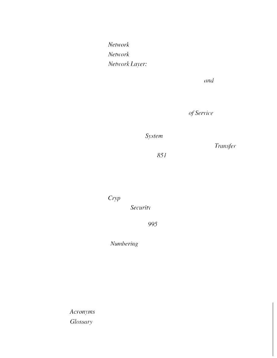
A data communications system has five components (see Figure 1.1).
Figure 1.1
Five components of data communication
Rule 1:
Rule 2:
Rule
n:
Protocol
Message
Medium
Protocol
Rule 1:
Rule 2:
Rulen:
I. Message.
The
message
is the information (data) to be communicated. Popular
forms of information include text, numbers, pictures, audio, and video.
Sender.
The
sender
is the device that sends the data message. It can be a com-
puter, workstation, telephone handset, video camera, and so on.
Receiver.
The
receiver
is the device that receives the message.
It
can be a com-
puter, workstation, telephone handset, television, and so on.
Transmission medium.
The
transmission medium
is the physical path by which
a message travels from sender to receiver. Some examples of transmission media
include twisted-pair wire, coaxial cable, fiber-optic cable, and radio waves.

SECTION
1.1
DATA COMMUNICATIONS
5
5. Protocol. A protocol is a set of rules that govern data communications. It repre-
sents an agreement between the communicating devices. Without a protocol, two
devices may be connected but not communicating, just as a person speaking French
cannot be understood by a person who speaks only Japanese.
Data Representation
Information today comes in different forms such as text, numbers, images, audio, and
video.
Text
In data communications, text is represented as a bit pattern, a sequence of bits (Os or
Is). Different sets of bit patterns have been designed to represent text symbols. Each set
is called a code, and the process of representing symbols is called coding. Today, the
prevalent coding system is called Unicode, which uses 32 bits to represent a symbol or
character used in any language in the world. The American Standard Code for Infor-
mation Interchange (ASCII), developed some decades ago in the United States, now
constitutes the first 127 characters in Unicode and is also referred to as Basic Latin.
Appendix A includes part of the Unicode.
Numbers
Numbers are also represented by bit patterns. However, a code such as ASCII is not used
to represent numbers; the number is directly converted to a binary number to simplify
mathematical operations. Appendix B discusses several different numbering systems.
Images
Images are also represented by bit patterns. In its simplest form, an image is composed
of a matrix of pixels (picture elements), where each pixel is a small dot. The size of the
pixel depends on the
resolution.
For example, an image can be divided into 1000 pixels
or 10,000 pixels. In the second case, there is a better representation of the image (better
resolution), but more memory is needed to store the image.
After an image is divided into pixels, each pixel is assigned a bit pattern. The size
and the value of the pattern depend on the image. For an image made of only black-
and-white dots (e.g., a chessboard), a I-bit pattern is enough to represent a pixel.
If
an image is not made of pure white and pure black pixels, you can increase the
size of the bit pattern to include gray scale. For example, to show four levels of gray
scale, you can use 2-bit patterns. A black pixel can be represented by 00, a dark gray
pixel by 01, a light gray pixel by 10, and a white pixel by 11.
There are several methods to represent color images. One method is called RGB,
so called because each color is made of a combination of three primary colors:
red,
green, and blue. The intensity of each color is measured, and a bit pattern is assigned to
it. Another method is called YCM, in which a color is made of a combination of three
other primary colors: yellow, cyan, and magenta.
Audio
Audio refers to the recording or broadcasting of sound or music. Audio is by nature
different from text, numbers, or images. It is continuous, not discrete. Even when we
6
CHAPTER
1
INTRODUCTION
use a microphone to change voice or music to an electric signal, we create a continuous
signal. In Chapters 4 and 5, we learn how to change sound or music to a digital or an
analog signal.
Video
Video refers to the recording or broadcasting of a picture or movie. Video can either be
produced as a continuous entity (e.g., by a TV camera), or it can be a combination of
images, each a discrete entity, arranged to convey the idea of motion. Again we can
change video to a digital or an analog signal, as we will see in Chapters 4 and 5.
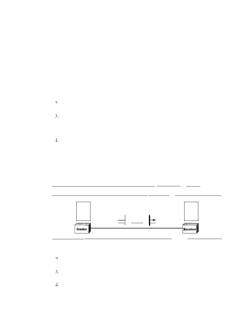
Data Flow
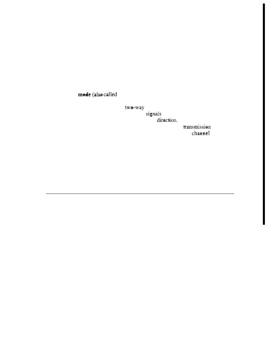
Communication between two devices can be simplex, half-duplex, or full-duplex as
shown in Figure 1.2.
Figure 1.2
Data flow (simplex, half-duplex, and full-duplex)
Mainframe
a. Simplex
b. Half-duplex
c. Full·duplex
Direction of data
Direction of data at time I
Direction of data at time 2
Direction of data all the time
)
Monitor
Simplex
In simplex mode, the communication is unidirectional, as on a one-way street. Only one
of the two devices on a link can transmit; the other can only receive (see Figure 1.2a).
Keyboards and traditional monitors are examples of simplex devices. The key-
board can only introduce input; the monitor can only accept output. The simplex mode
can use the entire capacity of the channel to send data in one direction.
Half-Duplex
In half-duplex mode, each station can both transmit and receive, but not at the same time. :
When one device is sending, the other can only receive, and vice versa (see Figure 1.2b).
SECTION
1.2
NETWORKS
7
The half-duplex mode is like a one-lane road with traffic allowed in both direc-
tions. When cars are traveling in one direction, cars going the other way must wait. In a
half-duplex transmission, the entire capacity of a channel is taken over by whichever of
the two devices is transmitting at the time. Walkie-talkies and CB (citizens band) radios
are both half-duplex systems.
The half-duplex mode is used in cases where there is no need for communication
in both directions at the same time; the entire capacity of the channel can be utilized for
each direction.
Full-Duplex
In
full-duplex
duplex),
both stations can transmit and receive simul-
taneously (see Figure 1.2c).
The full-duplex mode is like a
street with traffic flowing in both direc-
tions at the same time. In full-duplex mode,
going in one direction share the
capacity of the link: with signals going in the other
This sharing can occur in
two ways: Either the link must contain two physically separate
paths, one
for sending and the other for receiving; or the capacity of the
is divided
between signals traveling in both directions.
One common example of full-duplex communication is the telephone network.
When two people are communicating by a telephone line, both can talk and listen at the
same time.
The full-duplex mode is used when communication in both directions is required
all the time. The capacity of the channel, however, must be divided between the two
directions.
1.2
NETWORKS
A
network
is a set of devices (often referred to as nodes) connected by communication
links. A node can be a computer, printer, or any other device capable of sending and/or
receiving data generated by other nodes on the network.
Distributed Processing
Most networks use
distributed processing,
in which a task is divided among multiple
computers. Instead of one single large machine being responsible for all aspects of a
process, separate computers (usually a personal computer or workstation) handle a
subset.
Network Criteria
A network must be able to meet a certain number of criteria. The most important of
these are performance, reliability, and security.
Performance
Performance
can be measured in many ways, including transit time and response time.
Transit time is the amount of time required for a message to travel from one device to

8
CHAPTER 1
INTRODUCTION
another. Response time is the elapsed time between an inquiry and a response. The per-
formance of a network depends on a number of factors, including the number of users,
the type of transmission medium, the capabilities of the connected hardware, and the
efficiency of the software.
Performance is often evaluated by two networking metrics: throughput and delay.
We often need more throughput and less delay. However, these two criteria are often
contradictory.
If
we
try
to send more data to the network, we may increase throughput
but we increase the delay because of traffic congestion in the network.
Reliability
In addition to accuracy of delivery, network reliability is measured by the frequency of
failure, the time it takes a link to recover from a failure, and the network's robustness in
a catastrophe.
Security
Network security issues include protecting data from unauthorized access, protecting
data from damage and development, and implementing policies and procedures for
recovery from breaches and data losses.
Physical Structures
Before discussing networks, we need to define some network attributes.
Type of Connection
A network is two or more devices connected through links. A link is a communications
pathway that transfers data from one device to another. For visualization purposes, it is
simplest to imagine any link as a line drawn between two points. For communication to
occur, two devices must be connected in some way to the same link at the same time.
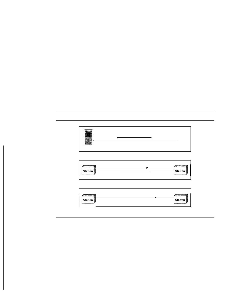
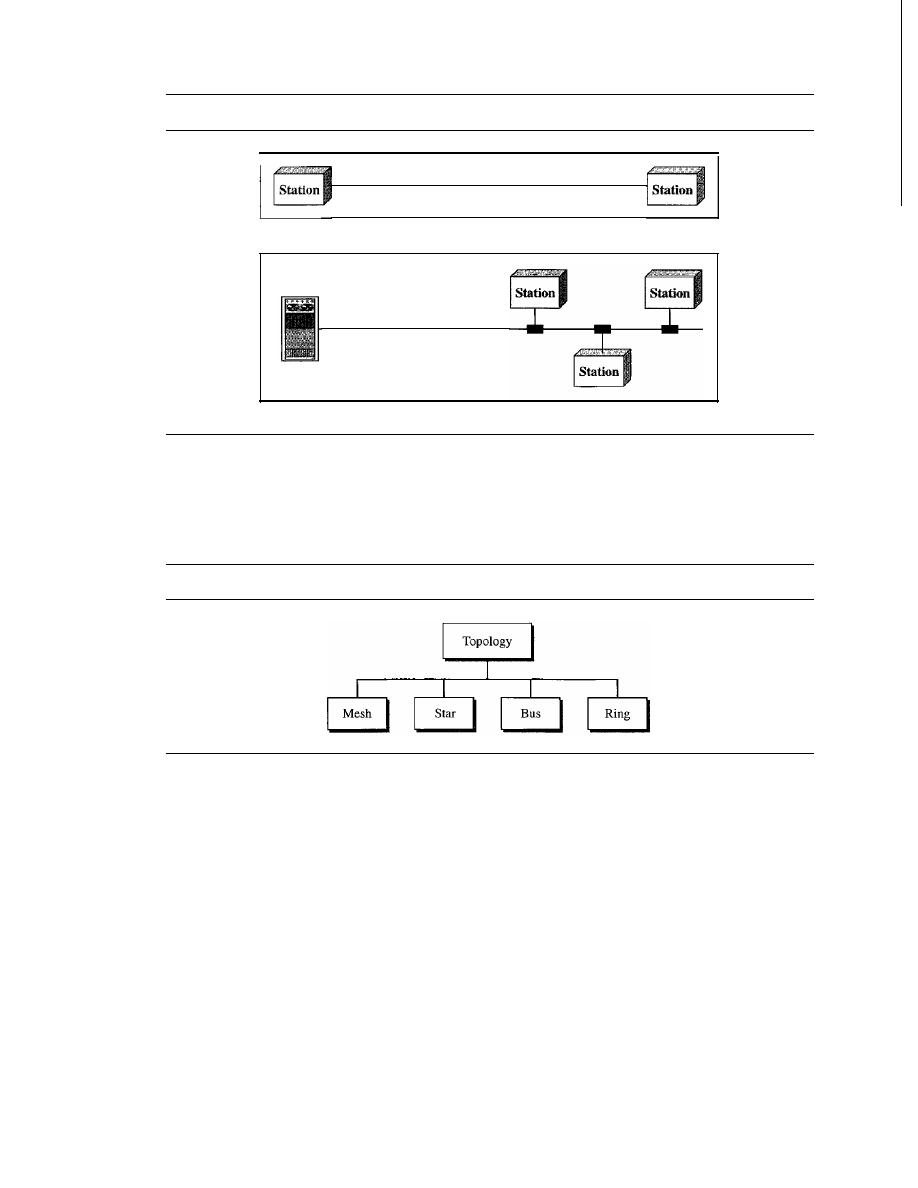
There are two possible types of connections: point-to-point and multipoint.
Point-to-Point
A point-to-point connection provides a dedicated link between two
devices. The entire capacity of the link is reserved for transmission between those two
devices. Most point-to-point connections use an actual length of wire or cable to con-
nect the two ends, but other options, such as microwave or satellite links, are also possi-
ble (see Figure 1.3a). When you change television channels by infrared remote control,
you are establishing a point-to-point connection between the remote control and the
television's control system.
Multipoint
A multipoint (also called multidrop) connection is one in which more
than two specific devices share a single link (see Figure 1.3b).
In a multipoint environment, the capacity of the channel is shared, either spatially
or temporally.
If
several devices can use the link simultaneously, it is a
spatially shared
connection. If users must take turns, it is a
timeshared
connection.
Physical Topology
The term physical topology refers to the way in which a network is laid out physically.:
or more devices connect to a link; two or more links form a topology. The topology
SECTION
1.2
NETWORKS
9
Figure 1.3
Types of connections: point-to-point and multipoint
Link
a. Point-to-point
Mainframe
Link
b. Multipoint
of a network is the geometric representation of the relationship of all the links and
linking devices (usually called
nodes) to one another. There are four basic topologies
possible: mesh, star, bus, and ring (see Figure 1.4).
Figure
1.4
Categories of topology
Mesh
In a
mesh topology, every device has a dedicated point-to-point link to every
other device. The term
dedicated
means that the link carries traffic only between the
two devices it connects. To find the number of physical links in a fully connected mesh
network with
n
nodes, we first consider that each node must be connected to every
other node. Node 1 must be connected to
n -
I nodes, node 2 must be connected to
n -
1
nodes, and finally node
n
must be connected to
n -
1 nodes. We need
n(n -
1) physical
links. However, if each physical link allows communication in both directions (duplex
mode), we can divide the number of links by 2. In other words, we can say that in a
mesh topology, we need
n(n
-1) /2
duplex-mode links.
To accommodate that many links, every device on the network must have
n -
1
input/output
(VO)
ports (see Figure 1.5) to be connected to the other
n - 1 stations.
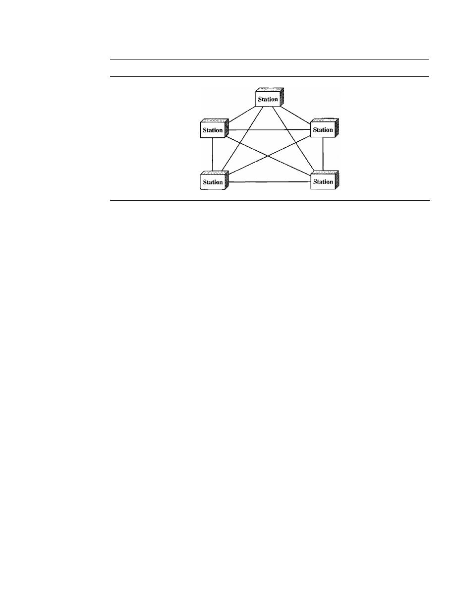
10
CHAPTER 1
INTRODUCTION
Figure 1.5
A fully connected mesh topology (five devices)
A mesh offers several advantages over other network topologies. First, the use of
dedicated links guarantees that each connection can carry its own data load, thus elimi-
nating the traffic problems that can occur when links must be shared by multiple devices.
Second, a mesh topology is robust.
If
one link becomes unusable, it does not incapaci-
tate the entire system. Third, there is the advantage of privacy or security. When every
message travels along a dedicated line, only the intended recipient sees it. Physical
boundaries prevent other users from gaining access to messages. Finally, point-to-point
links make fault identification and fault isolation easy. Traffic can be routed to avoid
links with suspected problems. This facility enables the network manager to discover the
precise location of the fault and aids in finding its cause and solution.
The main disadvantages of a mesh are related to the amount of cabling and the
number of I/O ports required. First, because every device must be connected to every
other device, installation and reconnection are difficult. Second, the sheer bulk of the
wiring can be greater than the available space (in walls, ceilings, or floors) can accom-
modate. Finally, the hardware required to connect each link (I/O ports and cable) can be
prohibitively expensive. For these reasons a mesh topology is usually implemented in a
limited fashion, for example, as a backbone connecting the main computers of a hybrid
network that can include several other topologies.
One practical example of a mesh topology is the connection of telephone regional
offices in which each regional office needs to be connected to every other regional office.
Star Topology
In a star topology, each device has a dedicated point-to-point link
only to a central controller, usually called a hub. The devices are not directly linked to
one another. Unlike a mesh topology, a star topology does not allow direct traffic
between devices. The controller acts as an exchange:
If
one device wants to send data to
another, it sends the data to the controller, which then relays the data to the other con-
nected device (see Figure 1.6) .
A star topology is less expensive than a mesh topology. In a star, each device needs
only one link and one I/O port to connect it to any number of others. This factor also
makes it easy to install and reconfigure. Far less cabling needs to be housed, and addi-
tions, moves, and deletions involve only one connection: between that device and the hub.
Other advantages include robustness.
If
one link fails, only that link is affected. All
other links remain active. This factor also lends itself to easy fault identification and
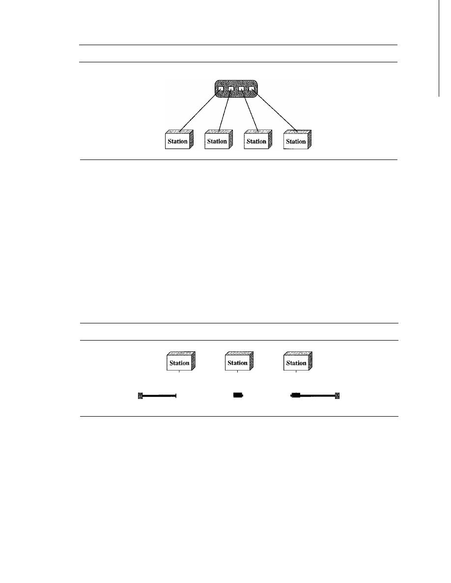
SECTION
1.2
NETWORKS
11
Figure 1.6
A star topology connecting four stations
Hub
fault isolation. As long as the hub is working, it can be used to monitor link problems
and bypass defective links.
One big disadvantage of a star topology is the dependency of the whole topology
on one single point, the hub. If the hub goes down, the whole system is dead.
Although a star requires far less cable than a mesh, each node must be linked to a
central hub. For this reason, often more cabling is required in a star than in some other
topologies (such as ring or bus).
The star topology is used in local-area networks (LANs), as we will see
in
Chapter 13.
High-speed LANs often use a star topology with a central hub.
Bus Topology
The preceding examples all describe point-to-point connections. A bus
topology, on the other hand, is multipoint. One long cable acts as a backbone to link all
the devices in a network (see Figure 1.7).
Figure 1.7
A bus topology connecting three stations
Drop line
Drop line
Drop line
Cable end
. .- - - - -
- - - - -
Cable end
Tap
Tap
Tap
Nodes are connected to the bus cable by drop lines and taps. A drop line is a con-
nection running between the device and the main cable. A tap is a connector that either
splices into the main cable or punctures the sheathing of a cable to create a contact with
the metallic core. As a signal travels along the backbone, some of its energy is transformed
into heat. Therefore, it becomes weaker and weaker as it travels farther and farther. For
this reason there is a limit on the number of taps a bus can support and on the distance
between those taps.
Advantages of a bus topology include ease of installation. Backbone cable can be
laid along the most efficient path, then connected to the nodes by drop lines of various
lengths. In this way, a bus uses less cabling than mesh or star topologies. In a star, for
example, four network devices in the same room require four lengths of cable reaching
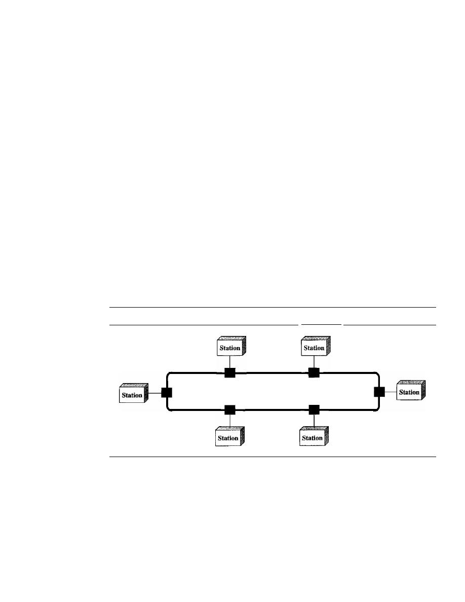
12
CHAPTER 1
INTRODUCTION
all the way to the hub. In a bus, this redundancy is eliminated. Only the backbone cable
stretches through the entire facility. Each drop line has to reach only as far as the near-
est point on the backbone.
Disadvantages include difficult reconnection and fault isolation. A bus is usually
designed to be optimally efficient at installation.
It
can therefore be difficult to add new
devices. Signal reflection at the taps can cause degradation in quality. This degradation
can be controlled by limiting the number and spacing of devices connected to a given
length of cable. Adding new devices may therefore require modification or replacement
of the backbone.
In addition, a fault or break in the bus cable stops all transmission, even between
devices on the same side of the problem. The damaged area reflects signals back in the
direction of origin, creating noise in both directions.
Bus topology was the one of the first topologies used in the design of early local-
area networks. Ethernet LANs can use a bus topology, but they are less popular now for
reasons we will discuss in Chapter 13.
Ring Topology
In a ring topology, each device has a dedicated point-to-point con-
nection with only the two devices on either side of it. A signal is passed along the ring
in one direction, from device to device, until it reaches its destination. Each device in
the ring incorporates a repeater. When a device receives a signal intended for another
device, its repeater regenerates the bits and passes them along (see Figure 1.8).
Figure 1.8
A ring topology connecting six stations
Repeater
Repeater
Repeater
Repeater
Repeater
Repeater
A ring is relatively easy to install and reconfigure. Each device is linked to only its
immediate neighbors (either physically or logically). To add or delete a device requires
changing only two connections. The only constraints are media and traffic consider-
ations (maximum ring length and number of devices). In addition, fault isolation is sim-
plified. Generally in a ring, a signal is circulating at all times.
If
one device does not
receive a signal within a specified period, it can issue an alarm. The alarm alerts the
network operator to the problem and its location.
However, unidirectional traffic can be a disadvantage. In a simple ring, a break in
the ring (such as a disabled station) can disable the entire network. This weakness can
be solved by using a dual ring or a switch capable of closing off the break.
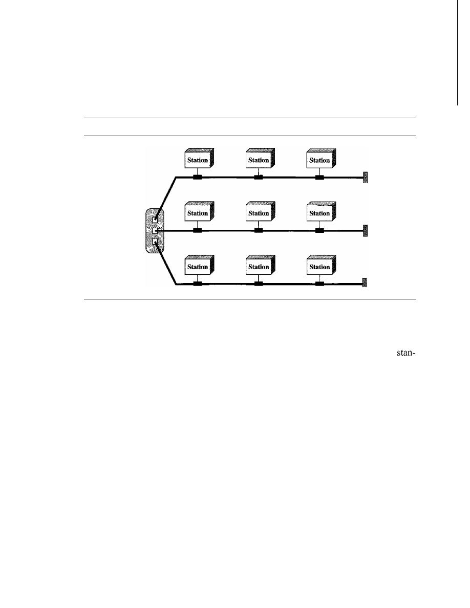
SECTION
1.2
NETWORKS
13
Ring topology was prevalent when IBM introduced its local-area network Token
Ring. Today, the need for higher-speed LANs has made this topology less popular.
Hybrid Topology
A network can be hybrid. For example, we can have a main star topol-
ogy with each branch connecting several stations in a bus topology as shown
in
Figure 1.9.
Figure 1.9
A
hybrid topology: a star backbone with three bus networks
Hub
Network Models
Computer networks are created by different entities. Standards are needed so that these
heterogeneous networks can communicate with one another. The two best-known
dards are the OSI model and the Internet model. In Chapter 2 we discuss these two
models. The OSI (Open Systems Interconnection) model defines a seven-layer net-
work; the Internet model defines a five-layer network. This book is based on the Internet
model with occasional references to the OSI model.
Categories of Networks
Today when we speak of networks, we are generally referring to two primary catego-
ries: local-area networks and wide-area networks. The category into which a network
falls is determined by its size. A LAN normally covers an area less than 2 mi; a WAN can
be worldwide. Networks of a size in between are normally referred to as metropolitan-
area networks and span tens of miles.
Local Area Network
A local area network (LAN) is usually privately owned and links the devices in a single
office, building, or campus (see Figure 1.10). Depending on the needs of an organization
and the type of technology used, a LAN can be as simple as two PCs and a printer in
someone's home office; or it can extend throughout a company and include audio and
video peripherals. Currently, LAN size is limited to a few kilometers.
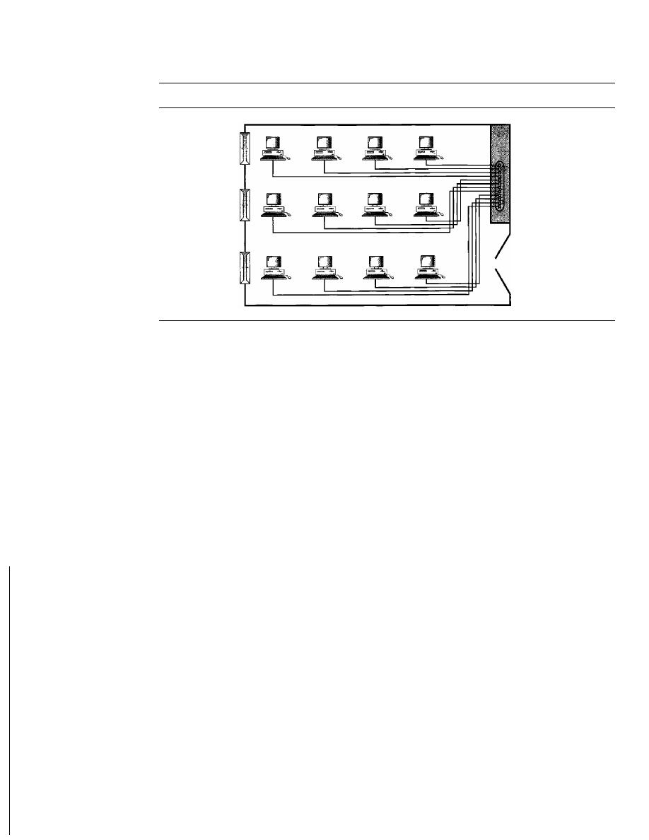
14
CHAPTER 1
INTRODUCTION
Figure 1.10
An isolated IAN connecting
12
computers to a hub in a closet
Hub
LANs are designed to allow resources to be shared between personal computers or
workstations. The resources to be shared can include hardware (e.g., a printer), software
(e.g., an application program), or data. A common example of a LAN, found in many
business environments, links a workgroup of task-related computers, for example, engi-
neering workstations or accounting PCs. One of the computers may be given a large-
capacity disk drive and may become a server to clients. Software can be stored on this
central server and used as needed by the whole group. In this example, the size of the
LAN may be determined by licensing restrictions on the number of users per copy of soft-
ware, or by restrictions on the number of users licensed to access the operating system.
In addition to size, LANs are distinguished from other types of networks by their
transmission media and topology. In general, a given LAN will use only one type of
transmission medium. The most common LAN topologies are bus, ring, and star.
Early LANs had data rates in the 4 to 16 megabits per second (Mbps) range. Today,
however, speeds are normally 100 or 1000 Mbps. LANs are discussed at length in
Chapters 13, 14, and 15.
Wireless LANs are the newest evolution in LAN technology. We discuss wireless
LANs in detail in Chapter 14.
Wide Area Network
A wide area network
(WAN)
provides long-distance transmission of data, image, audio,
and video information over large geographic areas that may comprise a country, a conti-
nent, or even the whole world. In Chapters
17
and
18
we discuss wide-area networks in
greater detail. A WAN can be as complex as the backbones that connect the Internet or as
simple as a dial-up line that connects a home computer to the Internet. We normally refer
to the first as a switched WAN and to the second as a point-to-point WAN (Figure 1.11).
The switched WAN connects the end systems, which usually comprise a router (internet-
working connecting device) that connects to another LAN or WAN. The point-to-point
WAN is normally a line leased from a telephone or cable TV provider that connects a
home computer or a small LAN to an Internet service provider (lSP). This type of WAN
is often used to provide Internet access.
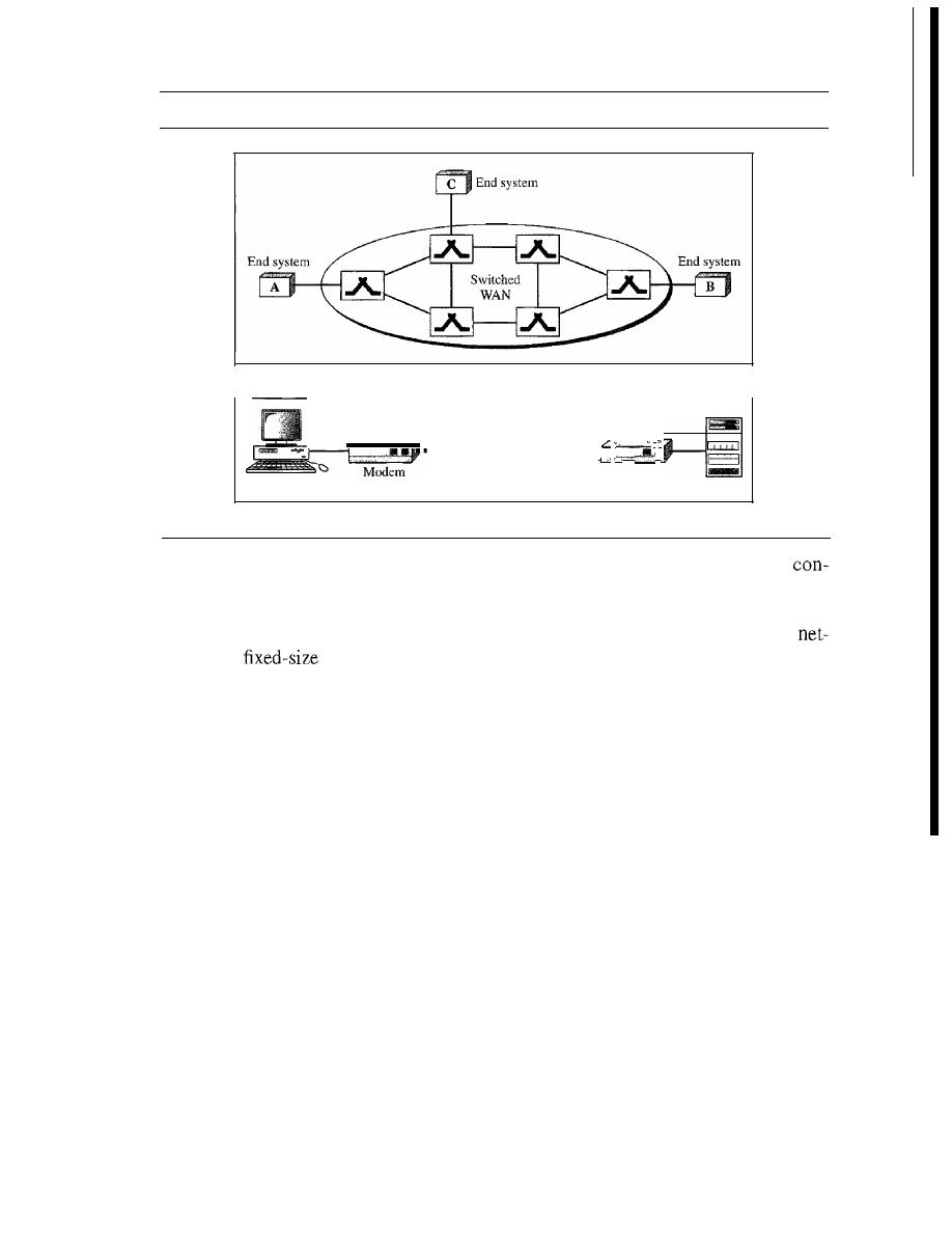
Computer
SECTION
1.2
NETWORKS
Figure 1.11
WANs: a switched WAN and a point-to-point WAN
a. Switched WAN
Point-te-point
:_:
WAN
"",
j
Modem
Modem
-
ISP
b.
Point-to-point WAN
15
i
i
I
An early example of a switched WAN is X.25, a network designed to provide
nectivity between end users. As we will see in Chapter 18, X.25 is being gradually
replaced by a high-speed, more efficient network called Frame Relay. A good example
of a switched WAN is the asynchronous transfer mode (ATM) network, which is a
work with
data unit packets called cells. We will discuss ATM in Chapter 18.
Another example ofWANs is the wireless WAN that is becoming more and more popu-
lar. We discuss wireless WANs and their evolution in Chapter 16.
Metropolitan Area Networks
A
metropolitan area network (MAN)
is a network with a size between a LAN and a
WAN. It normally covers the area inside a town or a city. It is designed for customers
who need a high-speed connectivity, normally to the Internet, and have endpoints
spread over a city or part of city. A good example of a MAN is the part of the telephone
company network that can provide a high-speed DSL line to the customer. Another
example is the cable TV network that originally was designed for cable TV, but today
can also be used for high-speed data connection to the Internet. We discuss DSL lines
and cable TV networks in Chapter
9.
Interconnection of Networks: Internetwork
Today, it is very rare to see a LAN, a MAN, or a LAN in isolation; they are con-
nected to one another. When two or more networks are connected, they become an
internetwork,
or
internet.
As an example, assume that an organization has two offices, one on the east coast
and the other on the west coast. The established office on the west coast has a bus topology
LAN; the newly opened office on the east coast has a star topology LAN. The president of
the company lives somewhere in the middle and needs to have control over the company
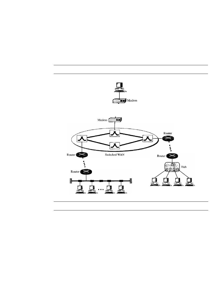
16
CHAPTER 1
INTRODUCTION
from her horne. To create a backbone WAN for connecting these three entities (two
LANs and the president's computer), a switched WAN (operated by a service provider
such as a telecom company) has been leased. To connect the LANs to this switched
WAN, however, three point-to-point WANs are required. These point-to-point WANs
can be a high-speed DSL line offered by a telephone company or a cable modern line
offered by a cable TV provider as shown in Figure 1.12.
Figure 1.12
A heterogeneous network made offour WANs and two LANs
President
•
•
Point-to-point:
WAN
:
•
•
Point-to-point
WAN
•
•
Point-to-point
WAN
.
LAN
LAN
1.3
THE INTERNET
The Internet has revolutionized many aspects of our daily lives.
It
has affected the way
we do business as well as the way we spend our leisure time. Count the ways you've
used the Internet recently. Perhaps you've sent electronic mail (e-mail) to a business
associate, paid a utility bill, read a newspaper from a distant city, or looked up a local
movie schedule-all by using the Internet. Or maybe you researched a medical topic,
booked a hotel reservation, chatted with a fellow Trekkie, or comparison-shopped for a
car. The Internet is a communication system that has brought a wealth of information to
our fingertips and organized it for our use.
The Internet is a structured, organized system. We begin with a brief history of the
Internet. We follow with a description of the Internet today.

SECTION
1.3
THE INTERNET
17
A Brief History
A network is a group of connected communicating devices such as computers and
printers. An internet (note the lowercase letter i) is two or more networks that can com-
municate with each other. The most notable internet is called the Internet (uppercase
letter I), a collaboration of more than hundreds of thousands of interconnected net-
works. Private individuals as well as various organizations such as government agen-
cies, schools, research facilities, corporations, and libraries in more than 100 countries
use the Internet. Millions of people are users. Yet this extraordinary communication sys-
tem only came into being in 1969.
In the mid-1960s, mainframe computers in research organizations were stand-
alone devices. Computers from different manufacturers were unable to communicate
with one another. The Advanced Research Projects Agency (ARPA) in the Depart-
ment of Defense (DoD) was interested in finding a way to connect computers so that
the researchers they funded could share their findings, thereby reducing costs and elim-
inating duplication of effort.
In 1967, at an Association for Computing Machinery (ACM) meeting, ARPA pre-
sented its ideas for ARPANET, a small network of connected computers. The idea was
that each host computer (not necessarily from the same manufacturer) would be
attached to a specialized computer, called an
message processor
(IMP). The
IMPs, in tum, would be connected to one another. Each IMP had to be able to commu-
nicate with other IMPs as well as with its own attached host.
By 1969, ARPANET was a reality. Four nodes, at the University of California at
Los Angeles (UCLA), the University of California at Santa Barbara (UCSB), Stanford
Research Institute (SRI), and the University of Utah, were connected via the IMPs to
form a network. Software called the
Network Control Protocol
(NCP) provided com-
munication between the hosts.
In 1972, Vint Cerf and Bob Kahn, both of whom were part of the core ARPANET
group, collaborated on what they called the
Internetting
Cerf and Kahn's land-
mark 1973 paper outlined the protocols to achieve end-to-end delivery of packets. This
paper on Transmission Control Protocol (TCP) included concepts such as encapsula-
tion, the datagram, and the functions of a gateway.
Shortly thereafter, authorities made a decision to split TCP into two protocols:
Transmission Control Protocol (TCP) and Internetworking Protocol (lP). IP would
handle datagram routing while TCP would be responsible for higher-level functions
such as segmentation, reassembly, and error detection. The internetworking protocol
became known as TCPIIP.
The Internet Today
The Internet has come a long way since the 1960s. The Internet today is not a simple
hierarchical structure.
It
is made up of many wide- and local-area networks joined by
connecting devices and switching stations.
It
is difficult to give an accurate represen-
tation of the Internet because it is continually changing-new networks are being
added, existing networks are adding addresses, and networks of defunct companies are
being removed. Today most end users who want Internet connection use the services of
Internet service providers (lSPs). There are international service providers, national
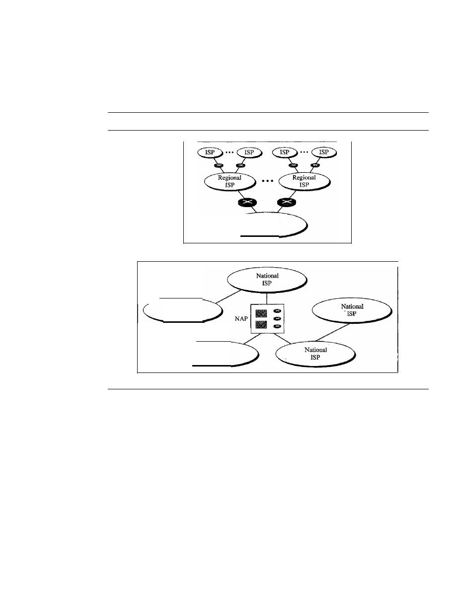
18
CHAPTER 1
INTRODUCTION
service providers, regional service providers, and local service providers. The Internet
today is run by private companies, not the government. Figure 1.13 shows a conceptual
(not geographic) view of the Internet.
Figure 1.13
Hierarchical organization of the Internet
National
ISP
a. Structure of a national ISP
National
ISP
National
ISP
b. Interconnection of national ISPs
International Internet Service Providers
At the top of the hierarchy are the international service providers that connect nations
together.
National Internet Service Providers
The national Internet service providers are backbone networks created and main-
tained by specialized companies. There are many national ISPs operating in North
America; some of the most well known are SprintLink, PSINet, UUNet Technology,
AGIS, and internet Mel. To provide connectivity between the end users, these back-
bone networks are connected by complex switching stations (normally run by a third
party) called network access points (NAPs). Some national ISP networks are also
connected to one another by private switching stations called
peering points.
These
normally operate at a high data rate (up to 600 Mbps).

SECTION
1.4
PROTOCOLS AND STANDARDS
19
Regional Internet Service Providers
Regional internet service providers or
regional ISPs
are smaller ISPs that are connected
to one or more national ISPs. They are at the third level of the hierarchy with a smaller
data rate.
Local Internet Service Providers
Local Internet service providers
provide direct service to the end users. The local
ISPs can be connected to regional ISPs or directly to national ISPs. Most end users are
connected to the local ISPs. Note that in this sense, a local ISP can be a company that
just provides Internet services, a corporation with a network that supplies services to its
own employees, or a nonprofit organization, such as a college or a university, that runs
its own network. Each of these local ISPs can be connected to a regional or national
service provider.
1.4
PROTOCOLS
AND STANDARDS
In this section, we define two widely used terms: protocols and standards. First, we
define protocol, which is synonymous with rule. Then we discuss standards, which are
agreed-upon rules.
Protocols
In computer networks, communication occurs between entities in different systems. An
entity
is anything capable of sending or receiving information. However, two entities can-
not simply send bit streams to each other and expect to be understood. For communication
to occur, the entities must agree on a protocol. A protocol is a set of rules that govern data
communications. A protocol defines what is communicated, how it is communicated, and
when it is communicated. The key elements of a protocol are syntax, semantics, and timing.
o
Syntax.
The term
syntax
refers to the structure or format of the data, meaning the
order in which they are presented. For example, a simple protocol might expect the
first 8 bits of data to be the address of the sender, the second 8 bits to be the address
of the receiver, and the rest of the stream to be the message itself.
o
Semantics.
The word
semantics
refers to the meaning of each section of bits.
How is a particular pattern to be interpreted, and what action is to be taken based
on that interpretation? For example, does an address identify the route to be taken
or the final destination of the message?
o
Timing.
The term
timing
refers to two characteristics: when data should be sent
and how fast they can be sent. For example, if a sender produces data at 100 Mbps
but the receiver can process data at only 1 Mbps, the transmission will overload the
receiver and some data will be lost.
Standards
Standards are essential in creating and maintaining an open and competitive market for
equipment manufacturers and in guaranteeing national and international interoperability
of data and telecommunications technology and processes. Standards provide guidelines

20
CHAPTER 1
INTRODUCTION
to manufacturers, vendors, government agencies, and other service providers to ensure
the kind of interconnectivity necessary in today's marketplace and in international com-
munications. Data communication standards fall into two categories: de facto (meaning
"by fact" or "by convention") and de jure (meaning "by law" or "by regulation").
o
De facto. Standards that have not been approved by an organized body but have
been adopted as standards through widespread use are de facto standards. De facto
standards are often established originally by manufacturers who seek to define the
functionality of a new product or technology.
o
De jure. Those standards that have been legislated by an officially recognized body
are de jure standards.
Standards Organizations
Standards are developed through the cooperation of standards creation committees,
forums, and government regulatory agencies.
Standards Creation Committees
While many organizations are dedicated to the establishment of standards, data tele-
communications in North America rely primarily on those published by the following:
o
International Organization for Standardization (ISO). The ISO is a multinational
body whose membership is drawn mainly from the standards creation committees
of various governments throughout the world. The ISO is active in developing
cooperation in the realms of scientific, technological, and economic activity.
o
International
Telecommunication
Union-Telecommunication
Standards
Sector (ITU-T). By the early 1970s, a number of countries were defining national
standards for telecommunications, but there was still little international compati-
bility. The United Nations responded by forming, as part of its International
Telecommunication Union (ITU), a committee, the Consultative Committee
for International Telegraphy and Telephony (CCITT). This committee was
devoted to the research and establishment of standards for telecommunications in
general and for phone and data systems in particular. On March 1, 1993, the name
of this committee was changed to the International Telecommunication Union-
Telecommunication Standards Sector (ITU-T).
o
American National Standards Institute (ANSI). Despite its name, the American
National Standards Institute is a completely private, nonprofit corporation not affili-
ated with the U.S. federal government. However, all ANSI activities are undertaken
with the welfare of the United States and its citizens occupying primary importance.
o
Institute of Electrical and Electronics Engineers (IEEE). The Institute of
Electrical and Electronics Engineers is the largest professional engineering society in
the world. International in scope, it aims to advance theory, creativity, and product
quality in the fields of electrical engineering, electronics, and radio as well as in all
related branches of engineering. As one of its goals, the IEEE oversees the develop-
ment and adoption of international standards for computing and communications.
o
Electronic Industries Association (EIA). Aligned with ANSI, the Electronic
Industries Association is a nonprofit organization devoted to the promotion of

SECTION
1.5
RECOMMENDED READING
21
electronics manufacturing concerns. Its activities include public awareness education
and lobbying efforts in addition to standards development. In the field of information
technology, the EIA has made significant contributions by defining physical connec-
tion interfaces and electronic signaling specifications for data communication.
Forums
Telecommunications technology development is moving faster than the ability of stan-
dards committees to ratify standards. Standards committees are procedural bodies and
by nature slow-moving. To accommodate the need for working models and agreements
and to facilitate the standardization process, many special-interest groups have
oped forums made up of representatives from interested corporations. The forums
work with universities and users to test, evaluate, and standardize new technologies. By
concentrating their efforts on a particular technology, the forums are able to speed
acceptance and use of those technologies in the telecommunications community. The
forums present their conclusions to the standards bodies.
Regulatory Agencies
All communications technology is subject to regulation by government agencies such
as the Federal Communications Commission (FCC) in the United States. The pur-
pose of these agencies is to protect the public interest by regulating radio, television,
and wire/cable communications. The FCC has authority over interstate and interna-
tional commerce as it relates to communications.
Internet Standards
An Internet standard is a thoroughly tested specification that is useful to and adhered
to by those who work with the Internet. It is a formalized regulation that must be fol-
lowed. There is a strict procedure by which a specification attains Internet standard
status. A specification begins as an Internet draft. An Internet draft is a working docu-
ment (a work in progress) with no official status and a 6-month lifetime. Upon recom-
mendation from the Internet authorities, a draft may be published as a Request for
Comment (RFC). Each RFC is edited, assigned a number, and made available to all
interested parties. RFCs go through maturity levels and are categorized according to
their requirement level.
1.5
RECOMMENDED READING
For more details about subjects discussed in this chapter, we recommend the following
books and sites. The items enclosed in brackets [...] refer to the reference list at the end
of the book.
Books
The introductory materials covered in this chapter can be found in [Sta04] and [PD03].
[Tan03] discusses standardization in Section 1.6.

22
CHAPTER
1
INTRODUCTION
Sites
The following sites are related to topics discussed in this chapter.
o
www.acm.org/sigcomm/sos.html
This site gives the status of
networking
standards.
o
www.ietf.org/
The Internet Engineering Task Force (IETF) home page.
RFCs
The following site lists all RFCs, including those related to IP and TCP. In future chap-
ters we cite the RFCs pertinent to the chapter material.
o
www.ietf.org/rfc.html
1.6
KEY TERMS
Advanced Research Projects
Agency (ARPA)
American National Standards
Institute (ANSI)
American Standard Code for
Information Interchange (ASCII)
ARPANET
audio
backbone
Basic Latin
bus topology
code
Consultative Committee for
International Telegraphy
and Telephony (CCITT)
data
data communications
de facto standards
de jure standards
delay
distributed processing
Electronic Industries Association (EIA)
entity
Federal Communications Commission
(FCC)
forum
full-duplex mode, or duplex
half-duplex mode
hub
image
Institute of Electrical and Electronics
Engineers (IEEE)
International Organization for
Standardization (ISO)
International Telecommunication
Union-Telecommunication
Standards Sector (ITU-T)
Internet
Internet draft
Internet service provider (ISP)
Internet standard
internetwork or internet
local area network (LAN)
local Internet service providers
mesh topology
message
metropolitan area network (MAN)
multipoint or multidrop connection
national Internet service provider
network

network access points (NAPs)
node
performance
physical topology
point-to-point connection
protocol
receiver
regional ISP
reliability
Request for Comment (RFC)
ROB
ring topology
security
semantics
1.7
SUMMARY
SECTION
1.7
SUMMARY
23
sender
simplex mode
star topology
syntax
telecommunication
throughput
timing
Transmission Control Protocol!
Internetworking Protocol (TCPIIP)
transmission medium
Unicode
video
wide area network (WAN)
YCM
o
Data communications are the transfer of data from one device to another via some
form of transmission medium.
o
A data communications system must transmit data to the correct destination in an
accurate and timely manner.
o
The five components that make up a data communications system are the message,
sender, receiver, medium, and protocol.
o
Text, numbers, images, audio, and video are different forms of information.
o
Data flow between two devices can occur in one of three ways: simplex, half-duplex,
or full-duplex.
o
A network is a set of communication devices connected by media links.
o
In a point-to-point connection, two and only two devices are connected by a
dedicated link. In a multipoint connection, three or more devices share a link.
o
Topology refers to the physical or logical arrangement of a network. Devices may
be arranged in a mesh, star, bus, or ring topology.
o
A network can be categorized as a local area network or a wide area network.
o
A LAN is a data communication system within a building, plant, or campus, or
between nearby buildings.
o
A WAN is a data communication system spanning states, countries, or the whole
world.
o
An internet is a network of networks.
o
The Internet is a collection of many separate networks.
o
There are local, regional, national, and international Internet service providers.
o
A protocol is a set of rules that govern data communication; the key elements of
a protocol are syntax, semantics, and timing.

24
CHAPTER
1
INTRODUCTION
o
Standards are necessary to ensure that products from different manufacturers can
work together as expected.
o
The ISO, ITD-T, ANSI, IEEE, and EIA are some of the organizations involved
in standards creation.
o
Forums are special-interest groups that quickly evaluate and standardize new
technologies.
o
A Request for Comment is an idea or concept that is a precursor to an Internet
standard.
1.8
PRACTICE SET
Review Questions
1. Identify the five components of a data communications system.
What are the advantages of distributed processing?
What are the three criteria necessary for an effective and efficient network?
4. What are the advantages of a multipoint connection over a point-to-point
connection?
5. What are the two types of line configuration?
6. Categorize the four basic topologies in terms of line configuration.
7. What is the difference between half-duplex and full-duplex transmission modes?
Name the four basic network topologies, and cite an advantage of each type.
9. For
n
devices in a network, what is the number of cable links required for a mesh,
ring, bus, and star topology?
10. What are some of the factors that determine whether a communication system is a
LAN or WAN?
1
I.
What is an internet? What is the Internet?
12. Why are protocols needed?
13. Why are standards needed?
Exercises
14. What is the maximum number of characters or symbols that can be represented by
Unicode?
15. A color image uses 16 bits to represent a pixel. What is the maximum number of
different colors that can be represented?
16. Assume six devices are arranged in a mesh topology. How many cables are needed?
How many ports are needed for each device?
17. For each of the following four networks, discuss the consequences if a connection fails.
a. Five devices arranged in a mesh topology
b. Five devices arranged in a star topology (not counting the hub)
c. Five devices arranged in a bus topology
d. Five devices arranged in a ring topology

SECTION 1.8
PRACTICE SET
25
18. You have two computers connected by an Ethernet hub at home. Is this a LAN, a
MAN, or a WAN? Explain your reason.
19. In the ring topology in Figure 1.8, what happens if one of the stations is unplugged?
20.
In the bus topology in Figure 1.7, what happens if one ofthe stations is unplugged?
21. Draw a hybrid topology with a star backbone and three ring networks.
22. Draw a hybrid topology with a ring backbone and two bus networks.
23. Performance is inversely related to delay. When you use the Internet, which of the
following applications are more sensitive to delay?
a. Sending an
b. Copying a file
c. Surfing the Internet
24. When a party makes a local telephone call to another party, is this a point-to-point
or multipoint connection? Explain your answer.
25. Compare the telephone network and the Internet. What are the similarities? What
are the differences?
Research Activities
26. Using the site \\iww.cne.gmu.edu/modules/network/osi.html, discuss the OSI model.
27. Using the site www.ansi.org, discuss ANSI's activities.
28. Using the site www.ieee.org, discuss IEEE's activities.
29. Using the site www.ietf.org/, discuss the different types of RFCs.


CHAPTER 2
Network Models
A network is a combination of hardware and software that sends data from one location
to another. The hardware consists of the physical equipment that carries signals from
one point of the network to another. The software consists of instruction sets that make
possible the services that we expect from a network.
We can compare the task of networking to the task of solving a mathematics problem
with a computer. The fundamental job of solving the problem with a computer is done
by computer hardware. However, this is a very tedious task if only hardware is involved.
We would need switches for every memory location to store and manipulate data. The
task is much easier if software is available. At the highest level, a program can direct
the problem-solving process; the details of how this is done by the actual hardware can
be left to the layers of software that are called by the higher levels.
Compare this to a service provided by a computer network. For example, the task
of sending an e-mail from one point in the world to another can be broken into several
tasks, each performed by a separate software package. Each software package uses the
services of another software package. At the lowest layer, a signal, or a set of signals, is
sent from the source computer to the destination computer.
In this chapter, we give a general idea of the layers of a network and discuss the
functions of each. Detailed descriptions of these layers follow in later chapters.
2.1
LAYERED TASKS
We use the concept of layers in our daily life. As an example, let us consider two
friends who communicate through postal maiL The process of sending a letter to a
friend would be complex if there were no services available from the post office. Fig-
ure 2.1 shows the steps in this task.
27
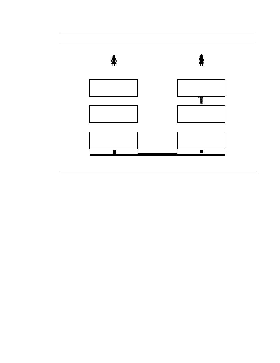
28
CHAPTER
2
NETWORK MODELS
Figure 2.1
Tasks involved in sending a letter
Sender
Receiver
I
t
The letter is written,
The letter is picked up,
put in an envelope, and
Higher layers
removed from the
dropped in a mailbox.
envelope, and read.
I
The letter is carried
The letter is carried
from the mailbox
Middle layers
from the post office
to a post office.
to the mailbox.
I
I
The letter is delivered
The letter is delivered
to
a carrier by the post
Lower layers
from the carrier
office.
to the post office.
The parcel is carried from
the source to the destination.
Sender, Receiver, and Carrier
In Figure 2.1 we have a sender, a receiver, and a carrier that transports the letter. There
is a hierarchy of tasks.
At the Sellder Site
Let us first describe, in order, the activities that take place at the sender site.
o
Higher layer. The sender writes the letter, inserts the letter in an envelope, writes
the sender and receiver addresses, and drops the letter in a mailbox.
o
Middle layer. The letter is picked up by a letter carrier and delivered to the post
office.
o
Lower layer. The letter is sorted at the post office; a carrier transports the letter.
011
the
Way
The letter is then on its way to the recipient. On the way to the recipient's local post
office, the letter may actually go through a central office. In addition, it may be trans-
ported by truck, train, airplane, boat, or a combination of these.
At the Receiver Site
o
Lower layer. The carrier transports the letter to the post office.
o
Middle layer. The letter is sorted and delivered to the recipient's mailbox.
o
Higher layer. The receiver picks up the letter, opens the envelope, and reads it.

SECTION 2.2
THE OS! MODEL
29
Hierarchy
According to our analysis, there are three different activities at the sender site and
another three activities at the receiver site. The task of transporting the letter between
the sender and the receiver is done by the carrier. Something that is not obvious
immediately is that the tasks must be done in the order given in the hierarchy. At the
sender site, the letter must be written and dropped in the mailbox before being picked
up by the letter carrier and delivered to the post office. At the receiver site, the letter
must be dropped in the recipient mailbox before being picked up and read by the
recipient.
Services
Each layer at the sending site uses the services of the layer immediately below it. The
sender at the higher layer uses the services of the middle layer. The middle layer uses
the services of the lower layer. The lower layer uses the services of the carrier.
The layered model that dominated data communications and networking literature
before 1990 was the Open Systems Interconnection (OSI) model. Everyone believed
that the OSI model would become the ultimate standard for data communications, but
this did not happen. The TCPIIP protocol suite became the dominant commercial archi-
tecture because it was used and tested extensively in the Internet; the OSI model was
never fully implemented.
In this chapter, first we briefly discuss the OSI model, and then we concentrate on
TCPIIP as a protocol suite.
2.2
THE OSI MODEL
Established in 1947, the International Standards Organization (ISO) is a multinational
body dedicated to worldwide agreement on international standards. An ISO standard
that covers all aspects of network communications is the Open Systems Interconnection
model. It was first introduced in the late 1970s. An open system is a set of protocols that
allows any two different systems to communicate regardless of their underlying archi-
tecture. The purpose of the OSI model is to show how to facilitate communication
between different systems without requiring changes to the logic of the underlying hard-
ware and software. The OSI model is not a protocol; it is a model for understanding and
designing a network architecture that is flexible, robust, and interoperable.
ISO is the organization. OSI is the model.
The OSI model is a layered framework for the design of network systems that
allows communication between all types of computer systems. It consists of seven sep-
arate but related layers, each of which defines a part of the process of moving information
across a network (see Figure 2.2). An understanding of the fundamentals of the OSI
model provides a solid basis for exploring data communications.

30
CHAPTER
2
NETWORK MODELS
Figure 2.2
Seven layers of the OSI model
71
Application
61
Presentation
51
Session
41
Transport
31
Network
21
Data link
1
I
Physical
Layered Architecture
The OSI model is composed of seven ordered layers: physical (layer 1), data link (layer 2),
network (layer 3), transport (layer 4), session (layer 5), presentation (layer 6), and
application (layer 7). Figure 2.3 shows the layers involved when a message is sent from
device A to device B. As the message travels from A to B, it may pass through many
intermediate nodes. These intermediate nodes usually involve only the first three layers
of the OSI model.
In
developing
the model, the designers distilled the process of transmitting data to
its most fundamental elements. They identified which networking functions had related
uses and collected those functions into discrete groups that became the layers. Each
layer defines a family of functions distinct from those of the other layers. By defining
and localizing functionality in this fashion, the designers created an architecture that is
both comprehensive and flexible. Most importantly, the OSI model allows complete
interoperability between otherwise incompatible systems.
Within a single machine, each layer calls upon the services of the layer just below
it. Layer 3, for example, uses the services provided by layer 2 and provides services for
layer 4. Between machines, layer
x
on one machine communicates with layer
x
on
another machine. This communication is governed by an agreed-upon series of rules
and conventions called protocols. The processes on each machine that communicate at
a given layer are called peer-to-peer processes. Communication between machines is
therefore a peer-to-peer process using the protocols appropriate to a given layer.
Peer-to-Peer
Processes
At the physical layer, communication is direct: In Figure 2.3, device A sends a stream
of bits to device B (through intermediate nodes). At the higher layers, however, com-
munication must move down through the layers on device A, over to device B, and then
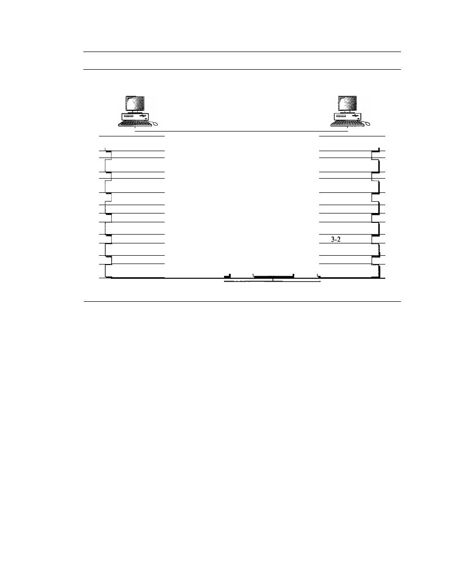
SECTION
2.2
THE OSI MODEL
31
Figure 2.3
The interaction between layers in the OSI model
Device
A
Device
B
Intermediate
node
Intermediate
node
Peer-to-peer protocol Oth layer)
7
Application
------------------------
Application
7
7-6 interface
7-6 interface
Peer-to-peer protocol (6th layer)
6
Presentation
------------------------
Presentation
6
6-5 interface
6-5 interface
Peer-to-peer protocol (5th layer)
5
Session
------------------------
Session
5
5-4 interface
Peer-to-peer protocol (4th layer)
5-4 interface
4
Transport
------------------------
Transport
4
4-3 interface
4-3 interface
3
Network
Network
3
3-2 interface
interface
2
Data link
Data link
2
2-1 interface
2-1 interface
Physical
Physical
Physical communication
back up through the layers. Each layer in the sending device adds its own information
to the message it receives from the layer just above it and passes the whole package to
the layer just below it.
At layer I the entire package is converted to a form that can be transmitted to the
receiving device. At the receiving machine, the message is unwrapped layer by layer,
with each process receiving and removing the data meant for it. For example, layer 2
removes the data meant for it, then passes the rest
to
layer 3. Layer 3 then removes the
data meant for it and passes the rest to layer 4, and so on.
Interfaces Between Layers
The passing of the data and network information down through the layers of the send-
ing device and back up through the layers of the receiving device is made possible by
an interface between each pair of adjacent layers. Each interface defines the informa-
tion and services a layer must provide for the layer above it. Well-defined interfaces and
layer functions provide modularity
to
a network. As long as a layer provides the
expected services to the layer above it, the specific implementation of its functions can
be modified or replaced without requiring changes to the surrounding layers.
Organization of the Layers
The seven layers can be thought of as belonging to three subgroups. Layers I, 2, and
3-physical, data link, and network-are the network support layers; they deal with
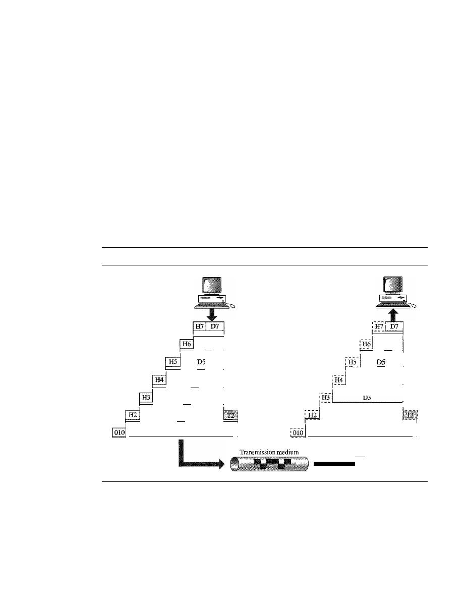
32
CHAPTER 2
NETWORK MODELS
the physical aspects of moving data from one device to another (such as electrical
specifications, physical connections, physical addressing, and transport timing and
reliability). Layers 5, 6, and 7-session, presentation, and application-can be
thought of as the user support layers; they allow interoperability among unrelated
software systems. Layer 4, the transport layer, links the two subgroups and ensures
that what the lower layers have transmitted is in a form that the upper layers can use.
The upper OSI layers are almost always implemented in software; lower layers are a
combination of hardware and software, except for the physical layer, which is mostly
hardware.
In Figure 2.4, which gives an overall view of the OSI layers, D7 means the data
unit at layer 7, D6 means the data unit at layer 6, and so on. The process starts at layer
7 (the application layer), then moves from layer to layer in descending, sequential
order. At each layer, a header, or possibly a trailer, can be added to the data unit.
Commonly, the trailer is added only at layer 2. When the formatted data unit passes
through the physical layer (layer 1), it is changed into an electromagnetic signal and
transported along a physical link.
Figure 2.4
An exchange using the OS! model
D6
I
D4
I
. - - - - - -
D3
I
D2
- -
010101010101101010000010000
I
1
D6
I
I
D4
I
D3
I
D2
010101010101101010000010000
I
Upon reaching its destination, the signal passes into layer 1 and is transformed
back into digital form. The data units then move back up through the OSI layers. As
each block of data reaches the next higher layer, the headers and trailers attached to it at
the corresponding sending layer are removed, and actions appropriate to that layer are
taken. By the time it reaches layer 7, the message is again in a form appropriate to the
application and is made available to the recipient.
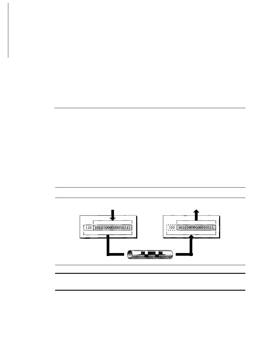
SECTION
2.3
LAYERS IN THE OSI MODEL
33
Encapsulation
Figure 2.3 reveals another aspect of data communications in the OSI model: encapsula-
tion. A packet (header and data) at level 7 is encapsulated in a packet at level 6. The
whole packet at level 6 is encapsulated in a packet at level 5, and so on.
In
other words, the data portion of a packet at level
N -
1 carries the whole packet
(data and header and maybe trailer) from level
N.
The concept is called encapsulation;
level
N -
1 is not aware of which part of the encapsulated packet is data and which part
is the header or trailer. For level
N -
1, the whole packet coming from level
N
is treated
as one integral unit.
2.3
LAYERS IN THE OSI MODEL
In this section we briefly describe the functions of each layer in the OSI model.
Physical Layer
The
physical layer
coordinates the functions required to carry a bit stream over a physi-
cal medium.
It
deals with the mechanical and electrical specifications of the interface and
transmission medium.
It
also defines the procedures and functions that physical devices
and interfaces have to perform for transmission to Occur. Figure 2.5 shows the position of
the physical layer with respect to the transmission medium and the data link layer.
Figure 2.5
Physical layer
From data link layer
To data link layer
Physical
layer
Physical
layer
Transmission medium
The physical layer is responsible for movements of
individual bits from one hop (node) to the next.
The physical layer is also concerned with the following:
o
Physical characteristics of interfaces and medium.
The physical layer defines
the characteristics of the interface between the devices and the transmission
medium.
It
also defines the type of transmission medium.
o
Representation of bits.
The physical layer data consists of a stream of
bits
(sequence of Os or 1s) with no interpretation. To be transmitted, bits must be
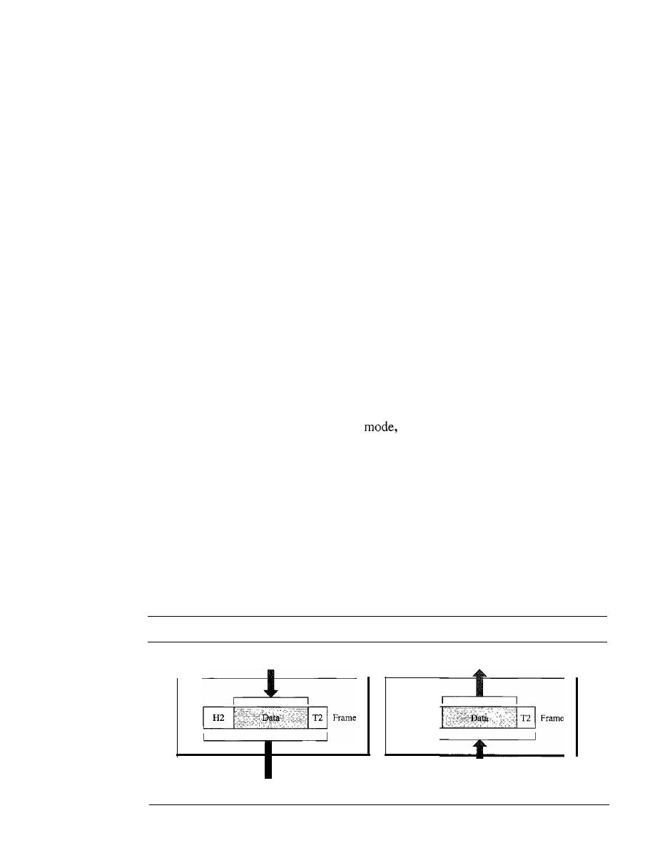
34
CHAPTER
2
NETWORK MODELS
encoded into signals--electrical or optical. The physical layer defines the type of
encoding (how Os and I s are changed to signals).
o
Data rate. The transmission rate-the number of bits sent each second-is also
defined by the physical layer. In other words, the physical layer defines the dura-
tion of a bit, which is how long it lasts.
o
Synchronization of bits. The sender and receiver not only must use the same bit
rate but also must be synchronized at the bit level. In other words, the sender and
the receiver clocks must be synchronized.
o
Line configuration. The physical layer is concerned with the connection of
devices to the media. In a point-to-point configuration, two devices are connected
through a dedicated link. In a multipoint configuration, a link is shared among
several devices.
o
Physical topology. The physical topology defines how devices are connected to
make a network. Devices can be connected by using a mesh topology (every device
is connected to every other device), a star topology (devices are connected through
a central device), a ring topology (each device is connected to the next, forming a
ring), a bus topology (every device is on a common link),
or
a hybrid topology (this
is a combination of two or more topologies).
o
Transmission mode. The physical layer also defines the direction of transmission
between two devices: simplex, half-duplex, or full-duplex. In simplex mode, only
one device can send; the other can only receive. The simplex mode is a one-way
communication. In the half-duplex
two devices can send and receive, but
not at the same time. In a full-duplex (or simply duplex) mode, two devices can
send and receive at the same time.
Data Link Layer
The data link layer transforms the physical layer, a raw transmission facility, to a reli-
able link.
It
makes the physical layer appear error-free to the upper layer (network
layer). Figure
2.6
shows the relationship of the data link layer to the network and phys-
icallayers.
Figure 2.6
Data link layer
From network layer
Data link layer
To physical layer
H2
To network layer
Data link layer
From physical layer
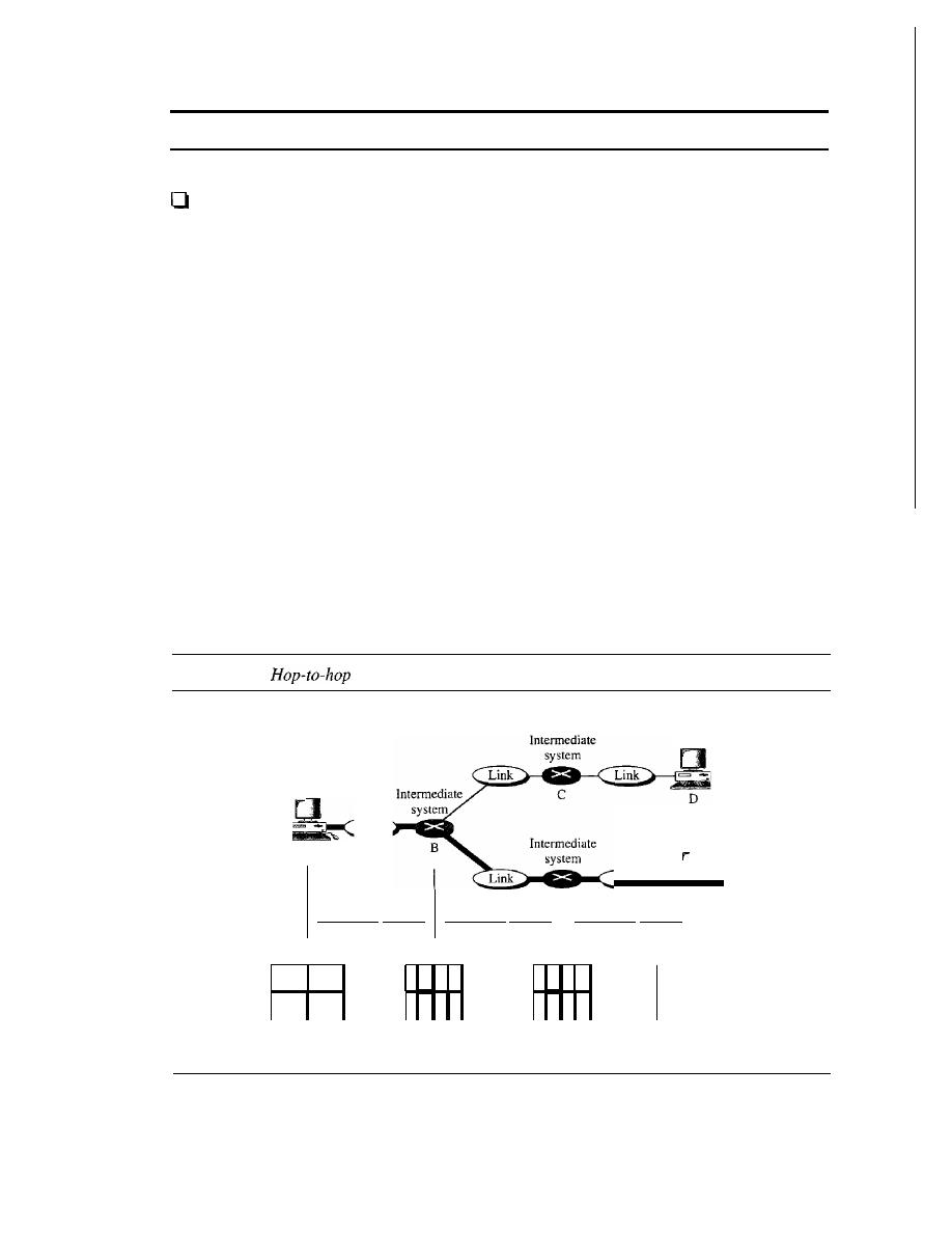
SECTION
2.3
LAYERS IN THE OSI MODEL
35
The data link layer is responsible for moving frames from one hop (node) to the next.
Other responsibilities of the data link layer include the following:
Framing.
The data link layer divides the stream of bits received from the network
layer into manageable data units called
frames.
o
Physical addressing.
If frames are to be distributed to different systems on the
network, the data link layer adds a header to the frame to define the sender and/or
receiver of the frame.
If
the frame is intended for a system outside the sender's
network, the receiver address is the address of the device that connects the network
to the next one.
D
Flow control.
If the rate at which the data are absorbed by the receiver is less than
the rate at which data are produced in the sender, the data link layer imposes a flow
control mechanism to avoid overwhelming the receiver.
o
Error control.
The data link layer adds reliability to the physical layer by adding
mechanisms to detect and retransmit damaged or lost frames.
It
also uses a mecha-
nism to recognize duplicate frames. Error control is normally achieved through a
trailer added to the end of the frame.
D
Access control.
When two or more devices are connected to the same link, data
link layer protocols are necessary to determine which device has control over the
link at any given time.
Figure 2.7 illustrates
hop-to-hop (node-to-node) delivery
by the data link layer.
Figure 2.7
delivery
End
system
Link
Link
A
End
system
End
system
E
F
Hop-ta-hop delivery
Hop-to-hop delivery
Hop-to-hop delivery
A
B
E
F
Data link
Data link
Data link
Physical
Physical
Physical
Hop-to-hop delivery
Hop-to-hop delivery
Hop-to-hop delivery
As the figure shows, communication at the data link layer occurs between two
adjacent nodes. To send data from A to F, three partial deliveries are made. First, the
data link layer at A sends a frame to the data link layer at B (a router). Second, the data
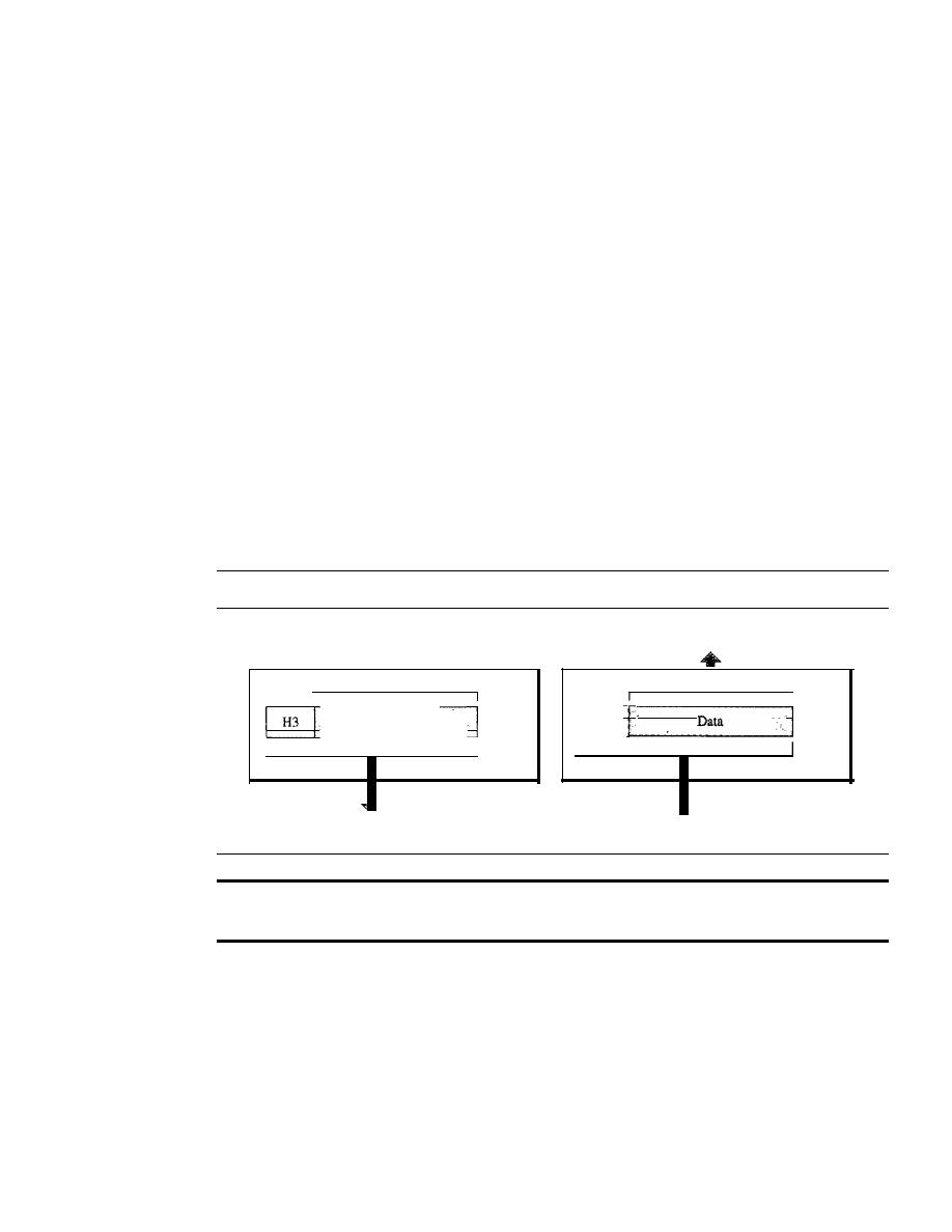
36
CHAPTER
2
NETWORK MODELS
link layer at B sends a new frame to the data link layer at E. Finally, the data link layer
at E sends a new frame to the data link layer at
F.
Note that the frames that are
exchanged between the three nodes have different values in the headers. The frame from
A to B has B as the destination address and A as the source address. The frame from B to
E has E as the destination address and B as the source address. The frame from E to F
has F as the destination address and E as the source address. The values of the trailers
can also be different if error checking includes the header of the frame.
Network Layer
The network layer is responsible for the source-to-destination delivery of a packet,
possibly across multiple networks (links). Whereas the data link layer oversees the
delivery of the packet between two systems on the same network (links), the network
layer ensures that each packet gets from its point of origin to its final destination.
If
two systems are connected to the same link, there is usually no need for a net-
work layer. However, if the two systems are attached to different networks (links) with
connecting devices between the networks (links), there is often a need for the network
layer to accomplish source-to-destination delivery. Figure 2.8 shows the relationship of
the network layer to the data link and transport layers.
Figure 2.8
Network layer
From transport layer
I
1
Data
Packet
I
I
To transport layer
I
',,- - -H-3- -
I
Packet
i------
Network
layer
To data link layer
Network
layer
From data link layer
The network layer is responsible for the delivery of individual
packets from the source host to the destination host.
Other responsibilities of the network layer include the following:
o
Logical addressing. The physical addressing implemented by the data link layer
handles the addressing problem locally. If a packet passes the network boundary,
we need another addressing system to help distinguish the source and destination
systems. The network layer adds a header to the packet coming from the upper
layer that, among other things, includes the logical addresses of the sender and
receiver. We discuss logical addresses later in this chapter.
o
Routing. When independent networks or links are connected to create
intemetworks
(network of networks) or a large network, the connecting devices (called
routers
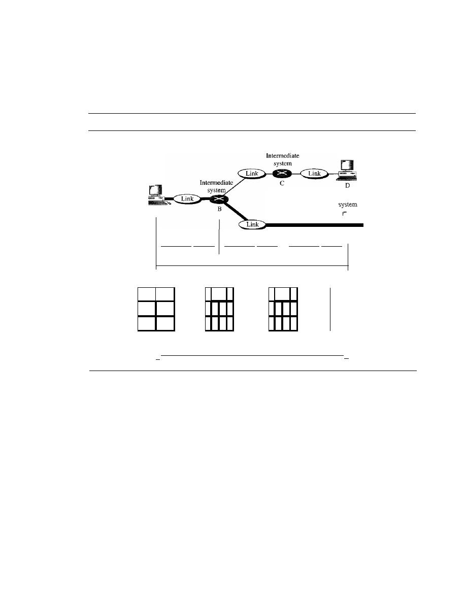
SECTION
2.3
LAYERS IN THE OSI MODEL
37
or
switches)
route or switch the packets to their final destination. One of the func-
tions of the network layer is to provide this mechanism.
Figure 2.9 illustrates end-to-end delivery by the network layer.
Figure 2.9
Source-to-destination delivery
End
Link
Intermediate
system
A
End
system
End
system
E
F
HOP-lO-hop delivery
Hop-to-hop delivery
HOp-lO-hop delivery
Source-to-destination delivery
A
B
E
F
Network
-
Network
-
Network
Data link
Data link
Data link
Physical
Physical
Physical
I.
Source-to-destination delivery
,I
As the figure shows, now we need a source-to-destination delivery. The network layer
at A sends the packet to the network layer at B. When the packet arrives at router B, the
router makes a decision based on the final destination (F) of the packet. As we will see
in later chapters, router B uses its routing table to find that the next hop is router
E.
The
network layer at B, therefore, sends the packet to the network layer at E. The network
layer at E, in tum, sends the packet to the network layer at F.
Transport Layer
The transport layer is responsible for process-to-process delivery of the entire mes-
sage. A process is an application program running on a host. Whereas the network layer
oversees source-to-destination delivery of individual packets, it does not recognize
any relationship between those packets.
It
treats each one independently, as though
each piece belonged to a separate message, whether or not it does. The transport layer,
on the other hand, ensures that the whole message arrives intact and in order, overseeing
both error control and flow control at the source-to-destination level. Figure 2.10 shows
the relationship of the transport layer to the network and session layers.
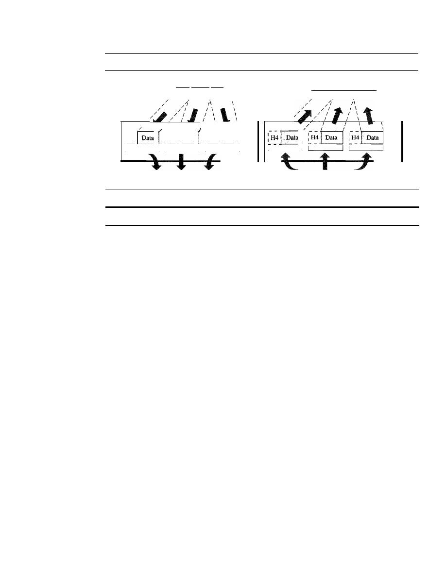
38
CHAPTER
2
NETWORK MODELS
Figure 2.10
Transport layer
From session layer
To session layer
\
\
\
\
Transport
layer
Segments
From network layer
/
/
I
I
I
To network layer
/
/
I
I
\
\
I
H4
I
H4
f
Data
I
H4)
Data
1
I
I I
I I
I
Segments
Transport
layer
The transport layer is responsible for the delivery of a message from one process to another.
Other responsibilities of the transport layer include the following:
o
Service-point addressing. Computers often run several programs at the same
time. For this reason, source-to-destination delivery means delivery not only from
one computer to the next but also from a specific process (running program) on
one computer to a specific process (running program) on the other. The transport
layer header must therefore include a type of address called a
service-point
address
(or port address). The network layer gets each packet to the correct
computer; the transport layer gets the entire message to the correct process on
that computer.
o
Segmentation and reassembly. A message is divided into transmittable segments,
with each segment containing a sequence number. These numbers enable the trans-
port layer to reassemble the message correctly upon arriving at the destination and
to identify and replace packets that were lost in transmission.
o
Connection control. The transport layer can be either connectionless or connection-
oriented. A connectionless transport layer treats each segment as an independent
packet and delivers it to the transport layer at the destination machine. A connection-
oriented transport layer makes a connection with the transport layer at the destina-
tion machine first before delivering the packets. After all the data are transferred,
the connection is terminated.
o
Flow control. Like the data link layer, the transport layer is responsible for flow
control. However, flow control at this layer is performed end to end rather than
across a single
link.
o
Error control. Like the data link layer, the transport layer is responsible for
error control. However, error control at this layer is performed process-to-
process rather than across a single link. The sending transport layer makes sure
that the entire message arrives at the receiving transport layer without
error
(damage, loss, or duplication). Error correction is usually achieved through
retransmission.
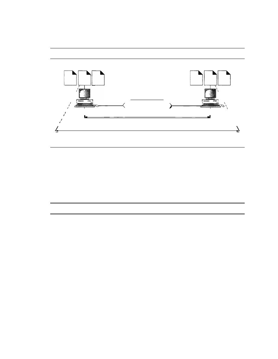
SECTION
2.3
LAYERS IN THE OSI MODEL
39
Figure 2.11 illustrates process-to-process delivery by the transport layer.
Figure 2.11
Reliable process-to-process delivery of a message
Processes
Processes
\
\
\
\
\
\
\
\
\
\
\
\
\
An internet
I
I
I
,,
,
,
I
I
I
I
,
I
Network layer
I
,
Host-to-host delivery
Transport layer
Process-to-process delivery
Session Layer
The services provided by the first three layers (physical, data link, and network) are
not sufficient for some processes. The session layer is the network
dialog controller.
It
establishes, maintains, and synchronizes the interaction among communicating
systems.
The session layer is responsible for dialog control and synchronization.
Specific responsibilities of the session layer include the following:
o
Dialog control. The session layer allows two systems to enter into a dialog.
It
allows the communication between two processes to take place in either half-
duplex (one way at a time) or full-duplex (two ways at a time) mode.
o
Synchronization. The session layer allows a process to add checkpoints, or syn-
Chronization points, to a stream of data. For example, if a system is sending a file
of 2000 pages, it is advisable to insert checkpoints after every 100 pages to ensure
that each 100-page unit is received and acknowledged independently. In this case,
if a crash happens during the transmission of page 523, the only pages that need to
be resent after system recovery are pages 501 to 523. Pages previous to 501 need
not be resent. Figure 2.12 illustrates the relationship of the session layer to the
transport and presentation layers.
Presentation Layer
The presentation layer is concerned with the syntax and semantics of the information
exchanged between two systems. Figure 2.13 shows the relationship between the pre-
sentation layer and the application and session layers.
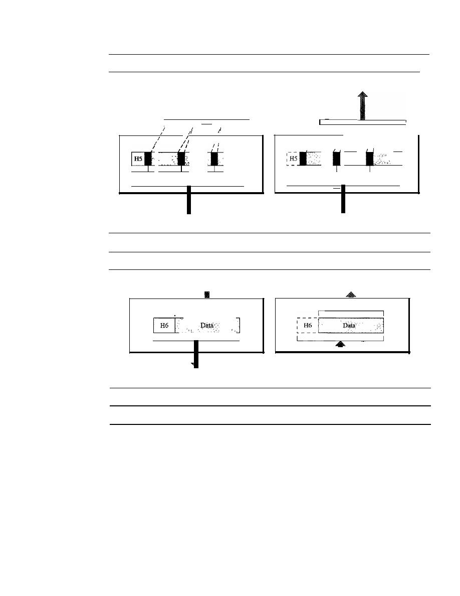
40
CHAPTER 2
NETWORK MODELS
Figure 2.12
Session layer
I
I
II
1/
I
I
I
I I
I I
I
I
I
I
syn
syn
syn
I
To presentation layer
I
I
I
I
I
I
I
I
I
From presentation layer
1
I
II
syn
syn
syn
1
Session
layer
Session
layer
To transport layer
From transport layer
Figure 2.13
Presentation layer
From application layer
To application layer
I
1
- - 1
I
I
Presentation
layer
To session layer
Presentation
layer
From session layer
The presentation layer is responsible for translation, compression, and encryption.
Specific responsibilities of the presentation layer include the following:
o
Translation.
The processes (running programs) in two systems are usually exchang-
ing information in the form of character strings, numbers, and so on. The infonna-
tion must be changed to bit streams before being transmitted. Because different
computers use different encoding systems, the presentation layer is responsible for
interoperability between these different encoding methods. The presentation layer
at the sender changes the information from its sender-dependent format into a
common format. The presentation layer at the receiving machine changes the
common format into its receiver-dependent format.
o
Encryption.
To carry sensitive information, a system must be able to ensure
privacy. Encryption means that the sender transforms the original information to
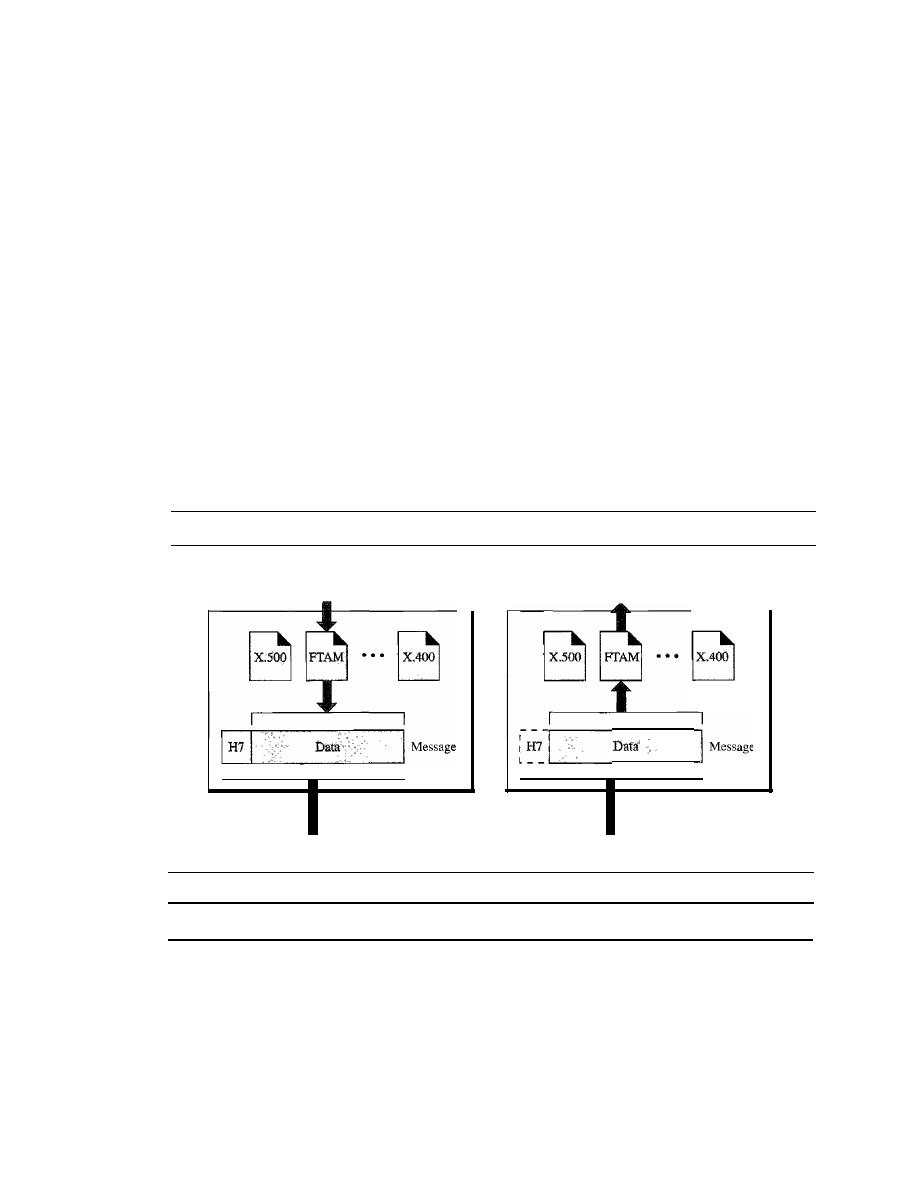
SECTION
2.3
LAYERS IN THE OSI MODEL
41
another form and sends the resulting message out over the network. Decryption
reverses the original process to transform the message back to its original form.
o
Compression. Data compression reduces the number of bits contained in the
information. Data compression becomes particularly important in the transmission
of multimedia such as text, audio, and video.
Application Layer
The application layer enables the user, whether human or software, to access the net-
work. It provides user interfaces and support for services such as electronic mail,
remote file access and transfer, shared database management, and other types of distrib-
uted information services.
Figure 2.14 shows the relationship of the application layer to the user and the pre-
sentation layer. Of the many application services available, the figure shows only three:
XAOO
(message-handling services), X.500 (directory services), and file transfer,
access, and management (FTAM). The user in this example employs
XAOO
to send an
e-mail message.
Figure 2.14
Application layer
User
(human or program)
Application
layer
To presentation layer
User
(human or program)
Application
layer
From presentation layer
The application layer is responsible for providing services to the user.
Specific services provided by the application layer include the following:
o
Network virtual terminal. A network virtual terminal is a software version of
a physical terminal, and it allows a user to log on to a remote host. To do so, the
application creates a software emulation of a terminal at the remote host. The
user's computer talks to the software terminal which, in turn, talks to the host,
and vice versa. The remote host believes it is communicating with one of its own
terminals and allows the user to log on.
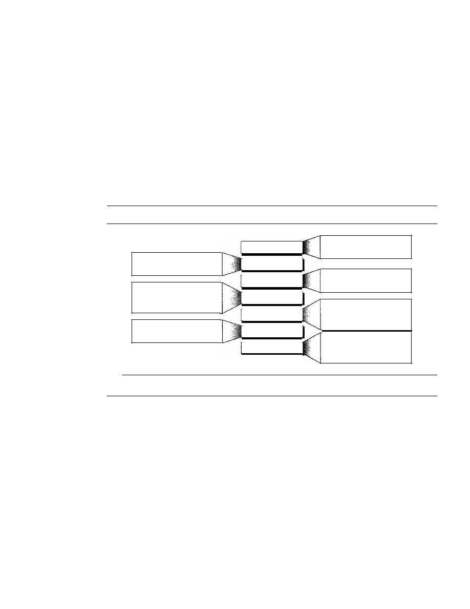
42
CHAPTER 2
NETWORK MODELS
o
File transfer, access,
and
management. This application allows a user to access
files in a remote host (to make changes or read data), to retrieve files from a remote
computer for use in the local computer, and to manage or control files in a remote
computer locally.
o
Mail services. This application provides the basis for e-mail forwarding and
storage.
o
Directory services. This application provides distributed database sources and
access for global information about various objects and services.
Summary of Layers
Figure 2.15 shows a summary of duties for each layer.
Figure
2.15
Summary of layers
To translate, encrypt, and
compress data
To provide reliable process-to-
process message delivery and
error recovery
To organize bits into frames;
to provide hop-to-hop delivery
Application
Presentation
Session
Transport
Network
Data link
Physical
To allow access to network
resources
To establish, manage, and
terminate sessions
To move packets from source
to destination; to provide
internetworking
To transmit bits over a medium;
to provide mechanical and
electrical specifications
2.4
TCP/IP PROTOCOL SUITE
The TCPIIP protocol suite was developed prior to the OSI model. Therefore, the lay-
ers in the TCP/IP protocol suite do not exactly match those in the OSI model. The
original TCP/IP protocol suite was defined as having four layers: host-to-network,
internet, transport, and application. However, when TCP/IP is compared to OSI, we can
say that the host-to-network layer is equivalent to the combination of the physical and
data link layers. The internet layer is equivalent to the network layer, and the applica-
tion layer is roughly doing the job of the session, presentation, and application layers
with the transport layer in TCPIIP taking care of part of the duties of the session layer.
So in this book, we assume that the TCPIIP protocol suite is made of five layers: physi-
cal, data link, network, transport, and application. The first four layers provide physical
standards, network interfaces, internetworking, and transport functions that correspond
to the first four layers of the OSI model. The three topmost layers in the OSI model,
however, are represented in TCPIIP by a single layer called the
application layer (see
Figure 2.16).
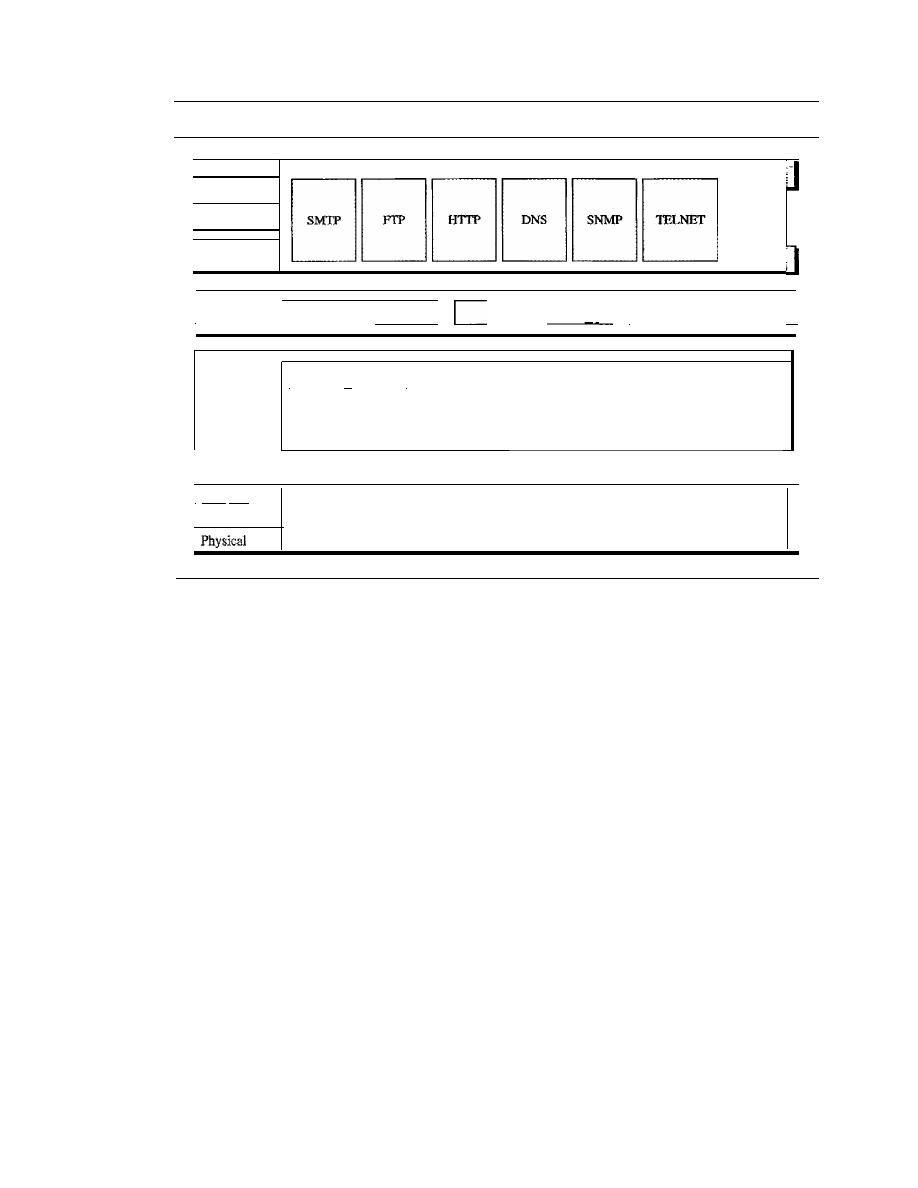
SECTION
2.4
TCPIIP PROTOCOL SUITE
43
Figure 2.16
TCPIIP and OSI model
I
Application
Applications
I
Presentation
...
]
I
Session
I
Transport
_ _ _
SC_TP_ _
!
__
TC_P
I I
UD_P_ _
II
I
ICMP
II
IGMP
I
Network
IP
(internet)
I
RARP
II
ARP
I
I
Data link
I
Protocols defined
by
the underlying networks
(host-to-network)
J
1
TCP/IP
is a hierarchical protocol made up of interactive modules, each of which
provides a specific functionality; however, the modules are not necessarily interdepen-
dent. Whereas the OSI model specifies which functions belong to each of its layers,
the layers of the
TCP/IP
protocol suite contain relatively independent protocols that
can be mixed and matched depending on the needs of the system. The term
hierarchi-
cal
means that each upper-level protocol is supported by one or more lower-level
protocols.
At the transport layer,
TCP/IP
defines three protocols: Transmission Control
Protocol (TCP), User Datagram Protocol (UDP), and Stream Control Transmission
Protocol (SCTP). At the network layer, the main protocol defined by TCP/IP is the
Internetworking Protocol (IP); there are also some other protocols that support data
movement in this layer.
Physical and Data Link Layers
At the physical and data link layers,
TCPIIP
does not define any specific protocol. It
supports all the standard and proprietary protocols. A network in a
TCPIIP
internetwork
can be a local-area network or a wide-area network.
Network Layer
At the network layer (or, more accurately, the internetwork layer),
TCP/IP
supports
the Internetworking Protocol. IP, in turn, uses four supporting protocols: ARP,
RARP, ICMP, and IGMP. Each of these protocols is described in greater detail in later
chapters.

44
CHAPTER
2
NETWORK MODELS
Internetworking Protocol (IP)
The Internetworking Protocol (IP) is the transmission mechanism used by the TCP/IP
protocols. It is an unreliable and connectionless protocol-a best-effort delivery service.
The term best effort means that IP provides no error checking or tracking. IP assumes
the unreliability of the underlying layers and does its best to get a transmission through
to its destination, but with no guarantees.
IP transports data in packets called datagrams, each of which is transported sepa-
rately. Datagrams can travel along different routes and can arrive out of sequence or be
duplicated. IP does not keep track of the routes and has no facility for reordering data-
grams once they arrive at their destination.
The limited functionality of IP should not be considered a weakness, however. IP
provides bare-bones transmission functions that free the user to add only those facilities
necessary for a given application and thereby allows for maximum efficiency. IP is dis-
cussed in Chapter 20.
Address Resolution Protocol
The Address Resolution Protocol (ARP) is used to associate a logical address with a
physical address. On a typical physical network, such as a LAN, each device on a link
is identified by a physical or station address, usually imprinted on the network interface
card (NIC). ARP is used to find the physical address of the node when its Internet
address is known. ARP is discussed in Chapter 21.
Reverse Address Resolution Protocol
The Reverse Address Resolution Protocol (RARP) allows a host to discover its Inter-
net address when it knows only its physical address. It is used when a computer is con-
nected to a network for the first time or when a diskless computer is booted. We discuss
RARP in Chapter 21.
Internet Control Message Protocol
The Internet Control Message Protocol (ICMP) is a mechanism used by hosts and
gateways to send notification of datagram problems back to the sender. ICMP sends
query and error reporting messages. We discuss ICMP in Chapter 21.
Internet Group Message Protocol
The Internet Group Message Protocol (IGMP) is used to facilitate the simultaneous
transmission of a message to a group of recipients. We discuss IGMP in Chapter 22.
Transport Layer
Traditionally the transport layer was represented in
TCP/IP
by two protocols: TCP and
UDP. IP is a host-to-host protocol, meaning that it can deliver a packet from one
physical device to another. UDP and TCP are transport level protocols responsible
for delivery of a message from a process (running program) to another process. A new
transport layer protocol, SCTP, has been devised to meet the needs of some newer
applications.
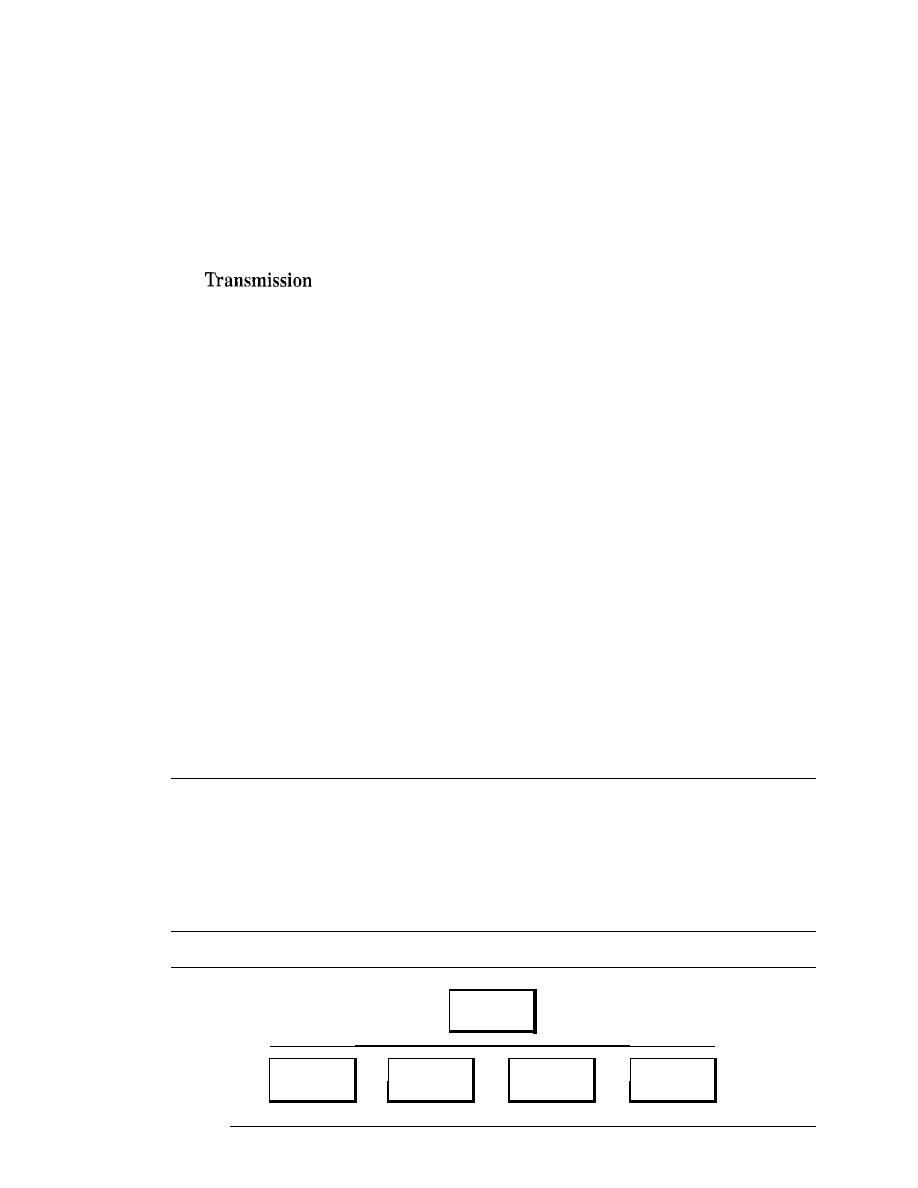
SECTION
2.5
ADDRESSING
45
User Datagram Protocol
The
User Datagram Protocol (UDP) is the simpler of the two standard TCPIIP transport
protocols.
It
is a process-to-process protocol that adds only port addresses, checksum
error control, and length information to the data from the upper layer. UDP is discussed
in Chapter 23.
Transmission Control Protocol
The
Control Protocol (TCP) provides full transport-layer services to
applications. TCP is a reliable stream transport protocol. The term
stream,
in this con-
text, means connection-oriented: A connection must be established between both ends
of a transmission before either can transmit data.
At the sending end of each transmission, TCP divides a stream of data into smaller
units called
segments.
Each segment includes a sequence number for reordering after
receipt, together with an acknowledgment number for the segments received. Segments
are carried across the internet inside of IP datagrams. At the receiving end, TCP col-
lects each datagram as it comes in and reorders the transmission based on sequence
numbers. TCP is discussed in Chapter 23.
Stream Control Transmission Protocol
The
Stream Control Transmission Protocol (SCTP) provides support for newer
applications such as voice over the Internet.
It
is a transport layer protocol that com-
bines the best features of UDP and TCP. We discuss SCTP in Chapter 23.
Application Layer
The
application layer
in TCPIIP is equivalent to the combined session, presentation,
and application layers in the OSI modeL Many protocols are defined at this layer. We
cover many of the standard protocols in later chapters.
2.5
ADDRESSING
Four levels of addresses are used in an internet employing the TCP/IP protocols:
physical (link) addresses, logical (IP) addresses, port addresses, and specific
addresses (see Figure 2.17).
Figure 2.17
Addresses in TCPIIP
Addresses
I
I
I
I
I
Physical
Logical
Port
Specific
addresses
addresses
addresses
addresses
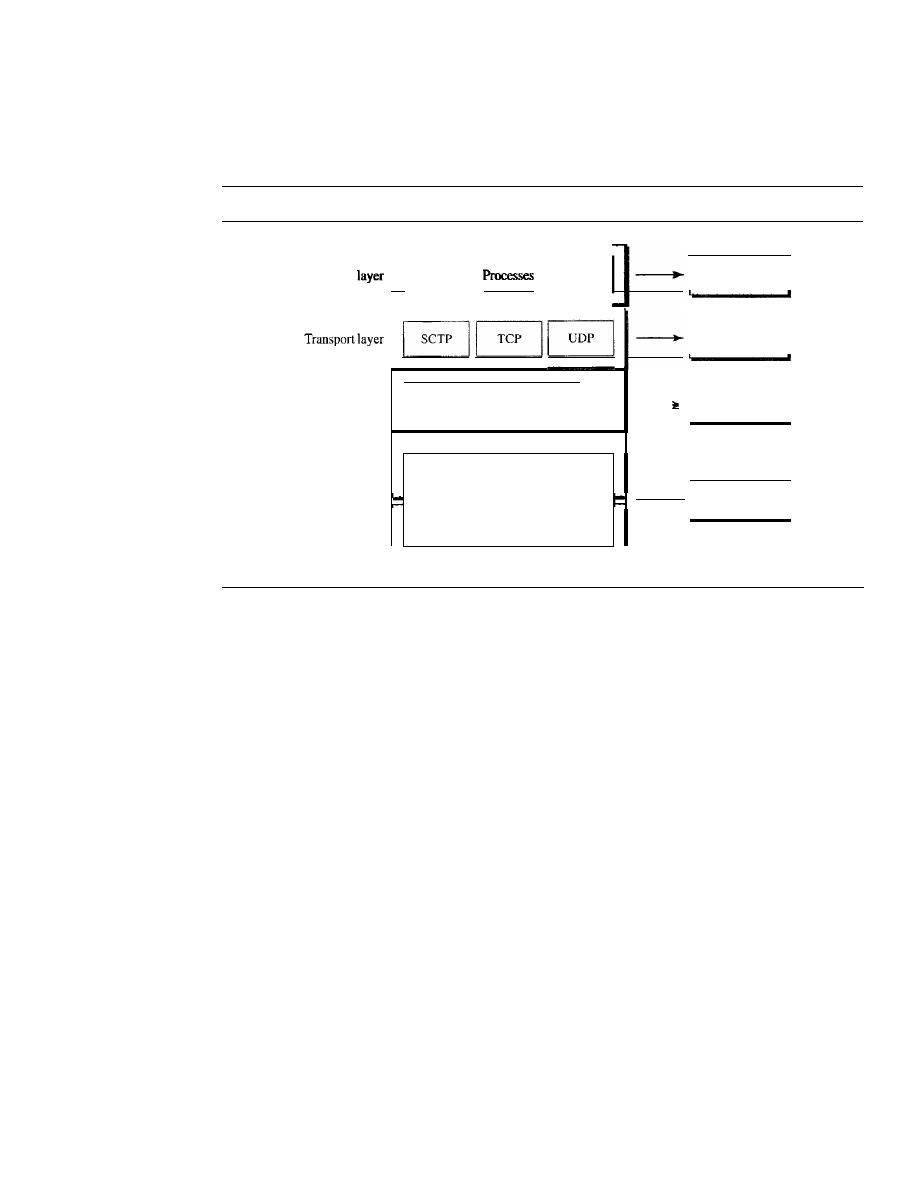
46
CHAPTER 2
NETWORK MODELS
Each address is related to a specific layer in the TCPIIP architecture, as shown in
Figure 2.18.
Figure 2.18
Relationship of layers and addresses in TCPIIP
Physical
addresses
Specific
addresses
Port
addresses
Logical
addresses
I
I
IPand
other protocols
Underlying
physical
networks
Physical layer
Appli"tio"
II
I
Network layer
Data link layer
Physical Addresses
The physical address, also known as the link address, is the address of a node as defined
by its LAN or WAN.
It
is included in the frame used by the data link layer.
It
is the
lowest-level address.
The physical addresses have authority over the network (LAN or WAN). The size
and format of these addresses vary depending on the network. For example, Ethernet
uses a 6-byte (48-bit) physical address that is imprinted on the network interface card
(NIC). LocalTalk (Apple), however, has a I-byte dynamic address that changes each
time the station comes up.
Example 2.1
In Figure 2.19 a node with physical address 10 sends a frame to a node with physical address 87.
The two nodes are connected by a link (bus topology LAN). At the data link layer, this frame
contains physical (link) addresses in the header. These are the only addresses needed. The rest of
the header contains other information needed at this level. The trailer usually contains extra bits
needed for error detection. As the figure shows, the computer with physical address lOis the
sender, and the computer with physical address 87 is the receiver. The data link layer at the
sender receives data from an upper layer.
It
encapsulates the data in a frame, adding a header and
a trailer. The header, among other pieces of information, carries the receiver and the sender phys-
ical (link) addresses. Note that in most data link protocols, the destination address, 87 in this
case, comes before the source address (10 in this case).
We have shown a bus topology for an isolated LAN. In a bus topology, the frame is propa-
gated in both directions (left and right). The frame propagated to the left dies when it reaches the
end of the cable if the cable end is terminated appropriately. The frame propagated to the right is
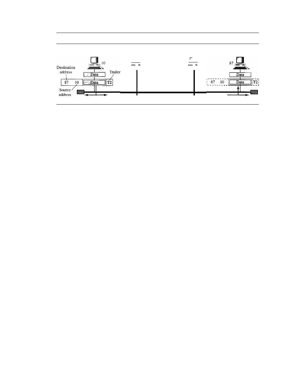
SECTION
2.5
ADDRESSING
47
Figure 2.19
Physical addresses
53
Sender
28
Destination address does
not match; the packet is
dropped
•••
LAN
Receiver
sent to every station on the network. Each station with a physical addresses other than 87 drops
the frame because the destination address in the frame does not match its own physical address.
The intended destination computer, however, finds a match between the destination address in the
frame and its own physical address. The frame is checked, the header and trailer are dropped, and
the data part is decapsulated and delivered to the upper layer.
Example 2.2
As we will see in Chapter 13, most local-area networks use a 48-bit (6-byte) physical address
written as 12 hexadecimal digits; every byte (2 hexadecimal digits) is separated by a colon, as
shown below:
07:01:02:01 :2C:4B
A 6-byte (12 hexadecimal digits) physical address
Logical Addresses
Logical addresses are necessary for universal communications that are independent of
underlying physical networks. Physical addresses are not adequate in an internetwork
environment where different networks can have different address formats. A universal
addressing system is needed in which each host can be identified uniquely, regardless
of the underlying physical network.
The logical addresses are designed for this purpose. A logical address in the Internet
is currently a 32-bit address that can uniquely define a host connected to the Internet. No
two publicly addressed and visible hosts on the Internet can have the same IP address.
Example 2.3
Figure 2.20 shows a part of an internet with two routers connecting three LANs. Each device
(computer or router) has a pair of addresses (logical and physical) for each connection. In this
case, each computer is connected to only one link and therefore has only one pair of addresses.
Each router, however, is connected to three networks (only two are shown in the figure). So each
router has three pairs of addresses, one for each connection. Although it may obvious that each
router must have a separate physical address for each connection, it may not be obvious why it
needs a logical address for each connection. We discuss these issues
in
Chapter 22 when we dis-
cuss routing.
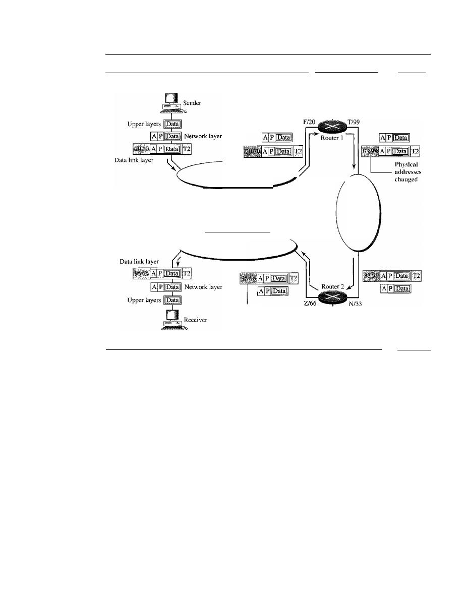
48
CHAPTER 2
NETWORK MODELS
Figure 2.20
IP addresses
AI
10
LAN 2
To another
network
Y/55
To another
XJ44
network
Ph)sical
addl'esscs
changed
LAN 3
LAN 1
P/95
The computer with logical address A and physical address 10 needs to send a
packet to the computer with logical address P and physical address 95. We use letters to
show the logical addresses and numbers for physical addresses, but note that both are
actually numbers, as we will see later in the chapter.
The sender encapsulates its data in a packet at the network layer and adds two logical
addresses (A and P). Note that in most protocols, the logical source address comes before
the logical destination address (contrary to the order of physical addresses). The network
layer, however, needs to find the physical address of the next hop before the packet can be
delivered. The network layer consults its routing table (see Chapter 22) and finds the
logical address of the next hop (router I) to be
F.
The ARP discussed previously finds
the physical address of router 1 that corresponds to the logical address of 20. Now the
network layer passes this address to the data link layer, which in tum, encapsulates the
packet with physical destination address 20 and physical source address 10.
The frame is received by every device on LAN 1, but is discarded by all except
router 1, which finds that the destination physical address in the frame matches with its
own physical address. The router decapsulates the packet from the frame to read the log-
ical destination address P. Since the logical destination address does not match the
router's logical address, the router knows that the packet needs to be forwarded. The

SECTION
2.5
ADDRESSING
49
router consults its routing table and ARP to find the physical destination address of the
next hop (router 2), creates a new frame, encapsulates the packet, and sends it to router 2.
Note the physical addresses in the frame. The source physical address changes
from 10 to 99. The destination physical address changes from 20 (router 1 physical
address) to 33 (router 2 physical address). The logical source and destination addresses
must remain the same; otherwise the packet will be lost.
At router 2 we have a similar scenario. The physical addresses are changed, and a
new frame is sent to the destination computer. When the frame reaches the destination,
the packet is decapsulated. The destination logical address P matches the logical address
of the computer. The data are decapsulated from the packet and delivered to the upper
layer. Note that although physical addresses will change from hop to hop, logical
addresses remain the same from the source to destination. There are some exceptions to
this rule that we discover later in the book.
The physical addresses
will
change from hop to hop,
but the logical addresses usually remain the same.
Port Addresses
The IP address and the physical address are necessary for a quantity of data to travel
from a source to the destination host. However, arrival at the destination host is not the
final objective of data communications on the Internet. A system that sends nothing but
data from one computer to another is not complete. Today, computers are devices that
can run multiple processes at the same time. The end objective of Internet communica-
tion is a process communicating with another process. For example, computer A can
communicate with computer C by using TELNET. At the same time, computer A com-
municates with computer B by using the File Transfer Protocol (FTP). For these pro-
cesses to receive data simultaneously, we need a method to label the different processes.
In other words, they need addresses. In the TCPIIP architecture, the label assigned to a
process is called a port address. A port address in TCPIIP is 16 bits in length.
Example 2.4
Figure 2.21 shows two computers communicating via the Internet. The sending computer is run-
ning three processes at this time with port addresses a, b, and c. The receiving computer is running
two processes at this time with port addresses
j
and k. Process a in the sending computer needs to
communicate with process
j
in the receiving computer. Note that although both computers are
using the same application, FTP, for example, the port addresses are different because one is a client
program and the other is a server program, as we will see in Chapter 23. To show that data from
process a need to be delivered to process
j,
and not k, the transport layer encapsulates data from
the application layer in a packet and adds two port addresses (a and
j),
source and destination. The
packet from the transport layer is then encapsulated in another packet at the network layer with
logical source and destination addresses (A and P). Finally, this packet is encapsulated in a frame
with the physical source and destination addresses of the next hop. We have not shown the physi-
cal addresses because they change from hop to hop inside the cloud designated as the Internet.
Note that although physical addresses change from hop to hop, logical and port addresses remain
the same from the source to destination. There are some exceptions to this rule that we discuss
later in the book.
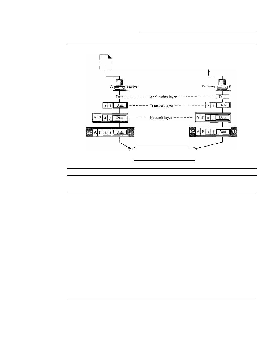
50
CHAPTER
2
NETWORK MODELS
Figure 2.21
Port addresses
a b c
DD
- - - - Data link layer - - - -
Internet
j
k
DD
The physical addresses change from hop to hop,
but the logical and port addresses usually remain the same.
Example 2.5
As we will see in Chapter 23, a port address is a 16-bit address represented by one decimal num-
her as shown.
753
A 16-bit port address represented as one single number
Specific Addresses
Some applications have user-friendly addresses that are designed for that specific address.
Examples include the e-mail address (for example, forouzan@fhda.edu) and the Universal
Resource Locator (URL) (for example, www.mhhe.com). The first defines the recipient of
an e-mail (see Chapter 26); the second is used to find a document on the World Wide Web
(see Chapter 27). These addresses, however, get changed to the corresponding port and
logical addresses by the sending computer, as we will see in Chapter 25.
2.6
RECOMMENDED READING
For more details about subjects discussed in this chapter, we recommend the following
books and sites. The items enclosed in brackets, [...] refer to the reference list at the
end of the text.

SECTION
2. 7
KEY TERMS
51
Books
Network models are discussed in Section 1.3 of [Tan03], Chapter 2 of [For06], Chapter 2
of [Sta04], Sections 2.2 and 2.3 of [GW04], Section 1.3 of [PD03], and Section 1.7 of
[KR05]. A good discussion about addresses can be found in Section 1.7 of [Ste94].
Sites
The following site is related to topics discussed in this chapter.
o
www.osi.org!
Information about OS1.
RFCs
The following site lists all RFCs, including those related to IP and port addresses.
o
www.ietLorg/rfc.html
2.7
KEY TERMS
access control
Address Resolution Protocol (ARP)
application layer
best-effort delivery
bits
connection control
data link layer
encoding
error
error control
flow control
frame
header
hop-to-hop delivery
host-to-host protocol
interface
Internet Control Message Protocol
(ICMP)
Internet Group Message Protocol (IGMP)
logical addressing
mail service
network layer
node-to-node delivery
open system
Open Systems Interconnection (OSI)
model
peer-to-peer process
physical addressing
physical layer
port address
presentation layer
process-to-process delivery
Reverse Address Resolution Protocol
(RARP)
routing
segmentation
session layer
source-to-destination delivery
Stream Control Transmission Protocol
(SCTP)
synchronization point
TCPIIP protocol suite
trailer
Transmission Control Protocol (TCP)
transmission rate
transport layer
transport level protocols
User Datagram Protocol (UDP)

52
CHAPTER 2
NETWORK MODELS
2.8
SUMMARY
o
The International Standards Organization created a model called the Open Systems
Interconnection, which allows diverse systems to communicate.
U
The seven-layer OSI model provides guidelines for the development of universally
compatible networking protocols.
o
The physical, data link, and network layers are the network support layers.
o
The session, presentation, and application layers are the user support layers.
D
The transport layer links the network support layers and the user support layers.
o
The physical layer coordinates the functions required to transmit a bit stream over
a physical medium.
o
The data link layer is responsible for delivering data units from one station to the
next without errors.
o
The network layer is responsible for the source-to-destination delivery of a packet
across multiple network links.
The transport layer is responsible for the process-to-process delivery of the entire
message.
D
The session layer establishes, maintains, and synchronizes the interactions between
communicating devices.
U
The presentation layer ensures interoperability between communicating devices
through transformation of data into a mutually agreed upon format.
o
The application layer enables the users to access the network.
TCP/IP is a five-layer hierarchical protocol suite developed before the OSI model.
U
The TCP/IP application layer is equivalent to the combined session, presentation,
and application layers of the OSI model.
U
Four levels of addresses are used in an internet following the TCP/IP protocols: phys-
ical (link) addresses, logical (IP) addresses, port addresses, and specific addresses.
o
The physical address, also known as the link address, is the address of a node as
defined by its LAN or WAN.
The IP address uniquely defines a host on the Internet.
The port address identifies a process on a host.
o
A specific address is a user-friendly address.
2.9
PRACTICE SET
Review Questions
I.
List the layers of the Internet model.
2. Which layers in the Internet model are the network support layers?
Which layer in the Internet model is the user support layer?
4. What is the difference between network layer delivery and transport layer delivery?

SECTION
2.9
PRACTICE SET
53
5. What is a peer-to-peer process?
6. How does information get passed from one layer to the next in the Internet
model?
7. What are headers and trailers, and how do they get added and removed?
What are the concerns of the physical layer in the Internet model?
9. What are the responsibilities of the data link layer in the Internet model?
10. What are the responsibilities of the network layer in the Internet model?
II.
What are the responsibilities of the transport layer in the Internet model?
What is the difference between a port address, a logical address, and a physical
address?
Name some services provided by the application layer in the Internet model.
How do the layers of the Internet model correlate to the layers of the OSI model?
Exercises
15. How are OSI and ISO related to each other?
16. Match the following to one or more layers of the OSI model:
a. Route determination
b. Flow control
c. Interface to transmission media
d. Provides access for the end user
I
7. Match the following to one or more layers of the OSI model:
a. Reliable process-to-process message delivery
b. Route selection
c. Defines frames
d. Provides user services such as e-mail and file transfer
e. Transmission of bit stream across physical medium
\
Match the following to one or more layers of the
OSl
model:
a. Communicates directly with user's application program
b. Error correction and retransmission
c. Mechanical, electrical, and functional interface
d. Responsibility for carrying frames between adjacent nodes
I
9. Match the following to one or more layers of the OSI model:
a. Format and code conversion services
b. Establishes, manages, and terminates sessions
c. Ensures reliable transmission of data
d. Log-in and log-out procedures
e. Provides independence from differences in data representation
In Figure 2.22, computer A sends a message to computer D via LANl, router Rl,
and LAN2. Show the contents of the packets and frames at the network and data
link layer for each hop interface.
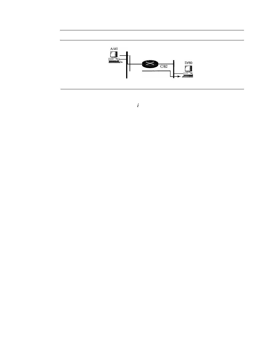
54
CHAPTER
2
NETWORK MODELS
Figure 2.22
Exercise 20
Sender
8/42
LAN 1
Rl
LAN 2
Sender
21. In Figure 2.22, assume that the communication is between a process running at
computer A with port address
and a process running at computer D with port
address
j.
Show the contents of packets and frames at the network, data link, and
transport layer for each hop.
22. Suppose a computer sends a frame to another computer on a bus topology LAN.
The physical destination address of the frame is corrupted during the transmission.
What happens to the frame? How can the sender be informed about the situation?
23. Suppose a computer sends a packet at the network layer to another computer
somewhere in the Internet. The logical destination address of the packet is cor-
rupted. What happens to the packet? How can the source computer be informed of
the situation?
24. Suppose a computer sends a packet at the transport layer to another computer
somewhere in the Internet. There is no process with the destination port address
running at the destination computer. What will happen?
25.
If
the data link layer can detect errors between hops, why do you think we need
another checking mechanism at the transport layer?
Research Activities
26. Give some advantages and disadvantages of combining the session, presentation,
and application layer in the OSI model into one single application layer in the
Internet model.
27. Dialog control and synchronization are two responsibilities of the session layer in
the OSI model. Which layer do you think is responsible for these duties in the
Internet model? Explain your answer.
28. Translation, encryption, and compression are some of the duties of the presentation
layer in the OSI model. Which layer do you think is responsible for these duties in
the Internet model? Explain your answer.
29. There are several transport layer models proposed in the OSI model. Find all of
them. Explain the differences between them.
30. There are several network layer models proposed in the OSI model. Find all of
them. Explain the differences between them.

Physical Layer
and Media
Objectives
We start the discussion of the Internet model with the bottom-most layer, the physical
layer. It is the layer that actually interacts with the transmission media, the physical part
of the network that connects network components together. This layer is involved in
physically carrying information from one node in the network to the next.
The physical layer has complex tasks to perform. One major task is to provide
services for the data link layer. The data in the data link layer consists of Os and I s orga-
nized into frames that are ready to be sent across the transmission medium. This stream
of Os and I s must first be converted into another entity: signals. One of the services pro-
vided by the physical layer is to create a signal that represents this stream of bits.
The physical layer must also take care of the physical network, the transmission
medium. The transmission medium is a passive entity; it has no internal program or
logic for control like other layers. The transmission medium must be controlled by the
physical layer. The physical layer decides on the directions of data flow. The physical
layer decides on the number of logical channels for transporting data coming from
different sources.
In Part 2 of the book, we discuss issues related to the physical layer and the trans-
mission medium that is controlled by the physical layer. In the last chapter of Part 2, we
discuss the structure and the physical layers of the telephone network and the cable
network.
Part 2 of the book is devoted to the physical layer
and the transmission media.

Chapters
This part consists of seven chapters: Chapters 3 to 9.
Chapter 3
Chapter 3 discusses the relationship between data, which are created by a device, and
electromagnetic signals, which are transmitted over a medium.
Chapter 4
Chapter 4 deals with digital transmission. We discuss how we can covert digital or
analog data to digital signals.
Chapter 5
Chapter 5 deals with analog transmission. We discuss how we can covert digital or
analog data to analog signals.
Chapter 6
Chapter 6 shows how we can use the available bandwidth efficiently. We discuss two
separate, but related topics, multiplexing and spreading.
Chapter 7
After explaining some ideas about data and signals and how we can use them effi-
ciently, we discuss the characteristics of transmission media, both guided and
unguided, in this chapter. Although transmission media operates under the physical
layer, they are controlled by the physical layer.
Chapter 8
Although the previous chapters in this part are issues related to the physical layer or
transmission media, Chapter 8 discusses switching, a topic that can be related to several
layers. We have included this topic in this part of the book to avoid repeating the dis-
cussion for each layer.
Chapter 9
Chapter 9 shows how the issues discussed in the previous chapters can be used in actual
networks. In this chapter, we first discuss the telephone network as designed to carry
voice. We then show how it can be used to carry data. Second, we discuss the cable
work as a television network. We then show how it can also be used to carry data.

CHAPTER 3
Data and Signals
One of the major functions of the physical layer is to move data in the form of electro-
magnetic signals across a transmission medium. Whether you are collecting numerical
statistics from another computer, sending animated pictures from a design workstation,
or causing a bell to ring at a distant control center, you are working with the transmis-
sion of data across network connections.
Generally, the data usable to a person or application are not in a form that can be
transmitted over a network. For example, a photograph must first be changed to a form
that transmission media can accept. Transmission media work by conducting energy
along a physical path.
To be transmitted, data must be transformed to electromagnetic signals.
3.1
ANALOG AND DIGITAL
Both data and the signals that represent them can be either analog or digital in form.
Analog and Digital Data
Data can be analog or digital. The term analog data refers to information that is contin-
uous; digital data refers to information that has discrete states. For example, an analog
clock that has hour, minute, and second hands gives information in a continuous form;
the movements of the hands are continuous. On the other hand, a digital clock that
reports the hours and the minutes will change suddenly from 8:05 to 8:06.
Analog data, such as the sounds made by a human voice, take on continuous values.
When someone speaks, an analog wave is created in the air. This can be captured by a
microphone and converted to an analog signal or sampled and converted to a digital
signal.
Digital data take on discrete values. For example, data are stored in computer
memory in the form of Os and 1s. They can be converted to a digital signal or modu-
lated into an analog signal for transmission across a medium.
57
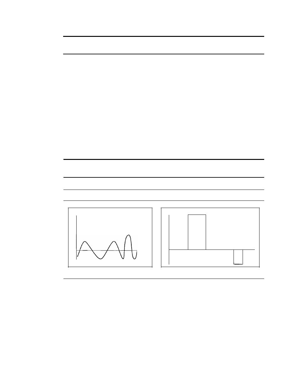
58
CHAPTER
3
DATA AND SIGNALS
Data can be analog or digital. Analog data are continuous and take continuous values.
Digital data have discrete states and take discrete values.
Analog and Digital Signals
Like the data they represent, signals can be either analog or digital. An analog signal
has infinitely many levels of intensity over a period of time. As the wave moves from
value
A
to value
B,
it passes through and includes an infinite number of values along its
path. A digital signal, on the other hand, can have only a limited number of defined
values. Although each value can be any number, it is often as simple as
1
and
O.
The simplest way to show signals is by plotting them on a pair of perpendicular
axes. The vertical axis represents the value or strength of a signal. The horizontal axis
represents time. Figure
3.1 illustrates an analog signal and a digital signal. The curve
representing the analog signal passes through an infinite number of points. The vertical
lines of the digital signal, however, demonstrate the sudden jump that the signal makes
from value to value.
Signals can be analog or digital. Analog signals can have an infinite number of
values in a range; digital signals can have only a limited number of values.
Figure 3.1
Comparison of analog and digital signals
Value
Value
Time
-
Time
a. Analog signal
b. Digital signal
Periodic and Nonperiodic Signals
Both analog and digital signals can take one of two forms:
periodic or nonperiodic
(sometimes refer to as
aperiodic, because the prefix a in Greek means "non").
A periodic signal completes a pattern within a measurable time frame, called a
period, and repeats that pattern over subsequent identical periods. The completion of
one full pattern is called a cycle. A nonperiodic signal changes without exhibiting a pat-
tern or cycle that repeats over time.
Both analog and digital signals can be periodic or nonperiodic. In data communi-
cations, we commonly use periodic analog signals (because they need less bandwidth,
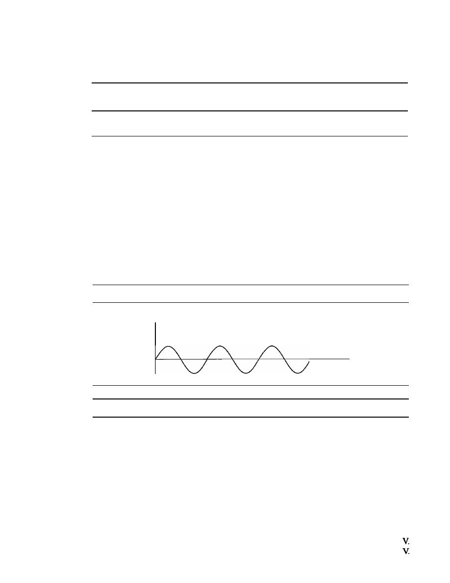
SECTION
3.2
PERIODIC ANALOG SIGNALS
59
as we will see in Chapter 5) and nonperiodic digital signals (because they can represent
variation in data, as we will see in Chapter 6).
In data communications, we commonly use periodic
analog signals and nonperiodic digital signals.
3.2
PERIODIC
ANALOG SIGNALS
Periodic analog signals can be classified as simple or composite. A simple periodic
analog signal, a sine wave, cannot be decomposed into simpler signals. A composite
periodic analog signal is composed of multiple sine waves.
Sine Wave
The sine wave is the most fundamental form of a periodic analog signal. When we
visualize it as a simple oscillating curve, its change over the course of a cycle is smooth
and consistent, a continuous, rolling flow. Figure 3.2 shows a sine wave. Each cycle
consists of a single arc above the time axis followed by a single arc below it.
Figure 3.2
A
sine wave
Value
Time
We discuss a mathematical approach to sine waves in Appendix C.
A sine wave can be represented by three parameters: the
peak amplitude,
the
fre-
quency,
and the
phase.
These three parameters fully describe a sine wave.
Peak Amplitude
The peak amplitude of a signal is the absolute value of its highest intensity, propor-
tional to the energy it carries. For electric signals, peak amplitude is normally measured
in
volts.
Figure 3.3 shows two signals and their peak amplitudes.
Example 3.1
The power in your house can be represented by a sine wave with a peak amplitude of 155 to 170
However, it is common knowledge that the voltage of the power in U.S. homes is 110 to 120
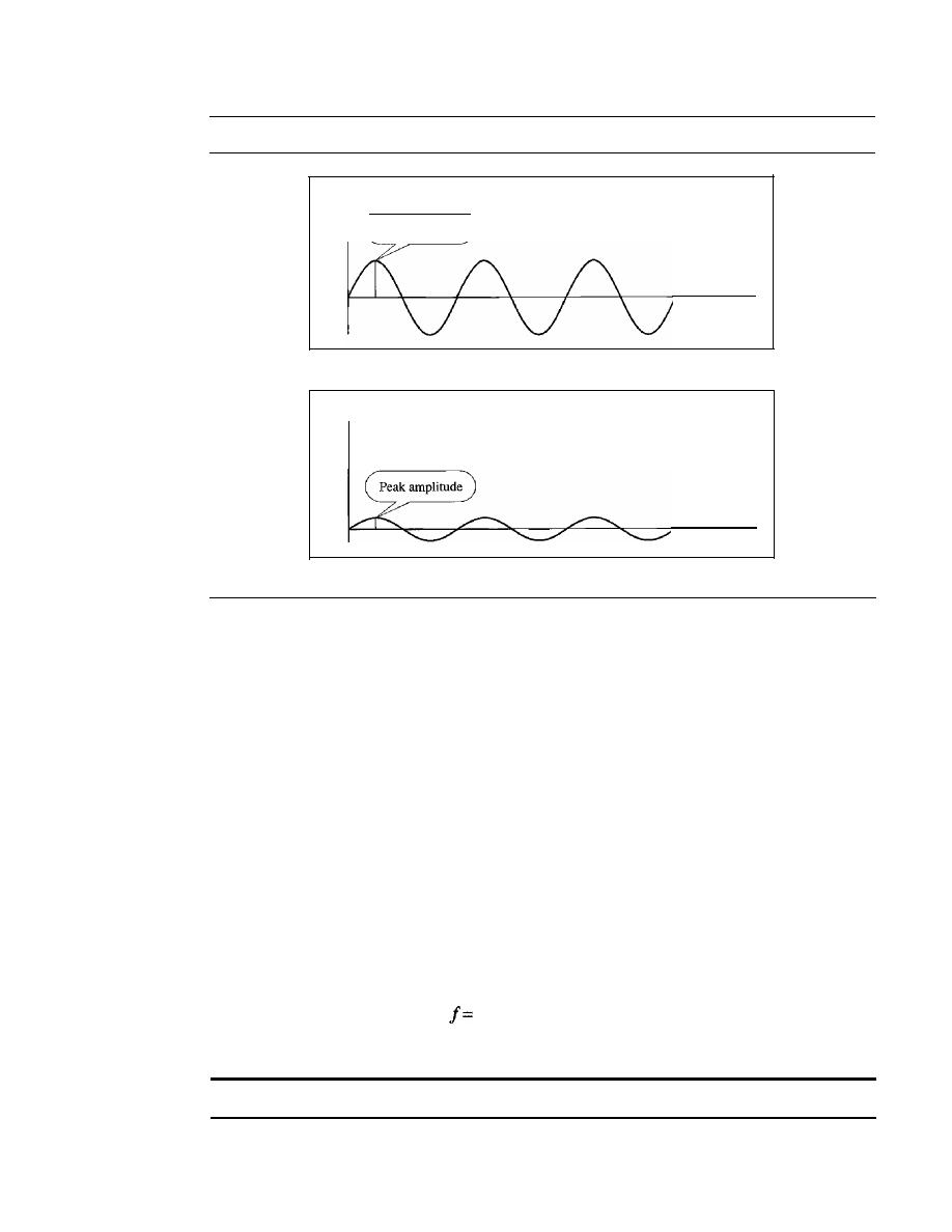
60
CHAPTER
3
DATA AND SIGNALS
Figure 3.3
Two signals with the same phase and frequency, but different amplitudes
Amplitude
Peak amplitude
Time
a. A signal with high peak amplitude
Amplitude
Time
b. A signal with low peak amplitude
This discrepancy is due to the fact that these are root mean square (rms) values. The signal is
squared and then the average amplitude is calculated. The peak value is equal to 2
112
x rms
value.
Example 3.2
The voltage of battery is a constant; this constant value can be considered a sine wave, as we will
see later. For example, the peak value of an AA battery is normally 1.5
V.
Period and Frequency
Period
refers to the amount of time, in seconds, a signal needs to complete 1 cycle.
Frequency
refers to the number of periods in
I
s. Note that period and frequency are just
one characteristic defined in two ways. Period is the inverse of frequency, and frequency
is the inverse of period, as the following formulas show.
1
-
T
and
1
T=-
f
Frequency and period are the inverse of each other.
Figure 3.4 shows two signals and their frequencies.
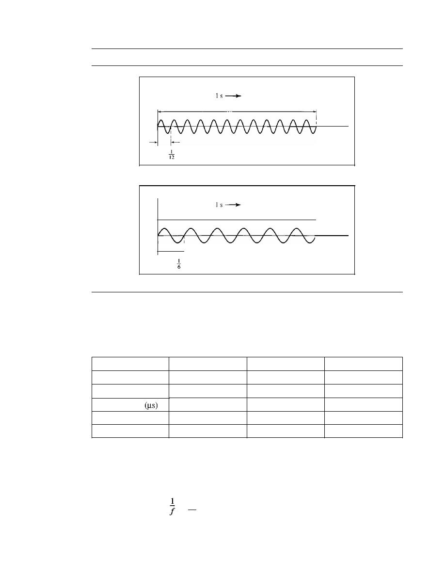
SECTION
3.2
PERIODIC ANALOG SIGNALS
61
Figure 3.4
Two signals with the same amplitude and phase, but different frequencies
Amplitude
12 periods in
Frequency is 12 Hz
1
s
Time
Period:
s
a. A signal with a frequency of 12 Hz
Amplitude
6 periods in
Frequency is 6 Hz
1
s
I
• • •
Time
T
Period:
s
b. A signal with a frequency of 6 Hz
Period is formally expressed in seconds. Frequency is formally expressed in
Hertz (Hz), which is cycle per second. Units of period and frequency are shown in
Table 3.1.
Table 3.1
Units ofperiod andfrequency
Unit
Equivalent
Unit
Equivalent
Seconds (s)
1 s
Hertz (Hz)
1 Hz
Milliseconds (ms)
10-
3
s
Kilohertz (kHz)
10
3
Hz
Microseconds
10-6 s
Megahertz (MHz)
10
6
Hz
Nanoseconds (ns)
10-
9
s
Gigahertz (GHz)
10
9
Hz
Picoseconds (ps)
10-
12
s
Terahertz (THz)
10
12
Hz
Example 3.3
The power we use at home has a frequency of
60
Hz
(50
Hz in Europe). The period of this sine
wave can be determined as follows:
T=
=
6
1
0
=
0.0166
s
=
0.0166
x
10
3
ms
=
16.6
illS
This means that the period of the power for our lights at home is 0.0116 s, or 16.6 ms. Our
eyes are not sensitive enough to distinguish these rapid changes in amplitude.

62
CHAPTER
3
DATA AND SIGNALS
Example 3.4
Express a period of
100
ms in microseconds.
Solution
From Table 3.1 we find the equivalents of 1 ms
(l
ms is 10-
3
s) and 1 s (1 sis
We make
the following substitutions:
100
100
X
10-
3
100
X
10-
3 X
10
6
10
2 X
10-
3 X
10
6
10
5
Example 3.5
The period of a signal is 100 ms. What is its frequency in kilohertz?
Solution
First we change lOO ms to seconds, and then we calculate the frequency from the period (1 Hz
=
10-
3
kHz).
100 ms
=
100
X
10-
3
S
=
10-
1
S
f=
= _1_
Hz
=
10
Hz
=
10
X
10-
3
kHz
=
10-
2
kHz
T
10-
1
More About Frequency
We already know that frequency is the relationship of a signal to time and that the frequency
of a wave is the number of cycles it completes in 1 s. But another way to look at frequency
is as a measurement of the rate of change. Electromagnetic signals are oscillating wave-
forms; that is, they fluctuate continuously and predictably above and below a mean energy
level. A 40-Hz signal has one-half the frequency of an 80-Hz signal; it completes 1 cycle
in
twice the time of the 80-Hz signal, so each cycle also takes twice as long to change from its
lowest to its highest voltage levels. Frequency, therefore, though described in cycles per sec-
ond (hertz), is a general measurement of the rate of change of a signal with respect to time.
Frequency is the rate of change with respect to time. Change in a short span of time
means high frequency. Change over a long span of time means low frequency.
If
the value of a signal changes over a very short span of time, its frequency is
high. If it changes over a long span of time, its frequency is low.
Two Extremes
What if a signal does not change at all? What
if
it maintains a constant voltage level for the
entire time it is active? In such a case, its frequency is zero. Conceptually, this idea is a sim-
ple one.
If
a signal does not change at all, it never completes a cycle, so its frequency is
a
Hz.
But what if a signal changes instantaneously? What if it jumps from one level to
another in no time? Then its frequency is infinite. In other words, when a signal changes
instantaneously, its period is zero; since frequency is the inverse of period, in this case,
the frequency is 1/0, or infinite (unbounded).
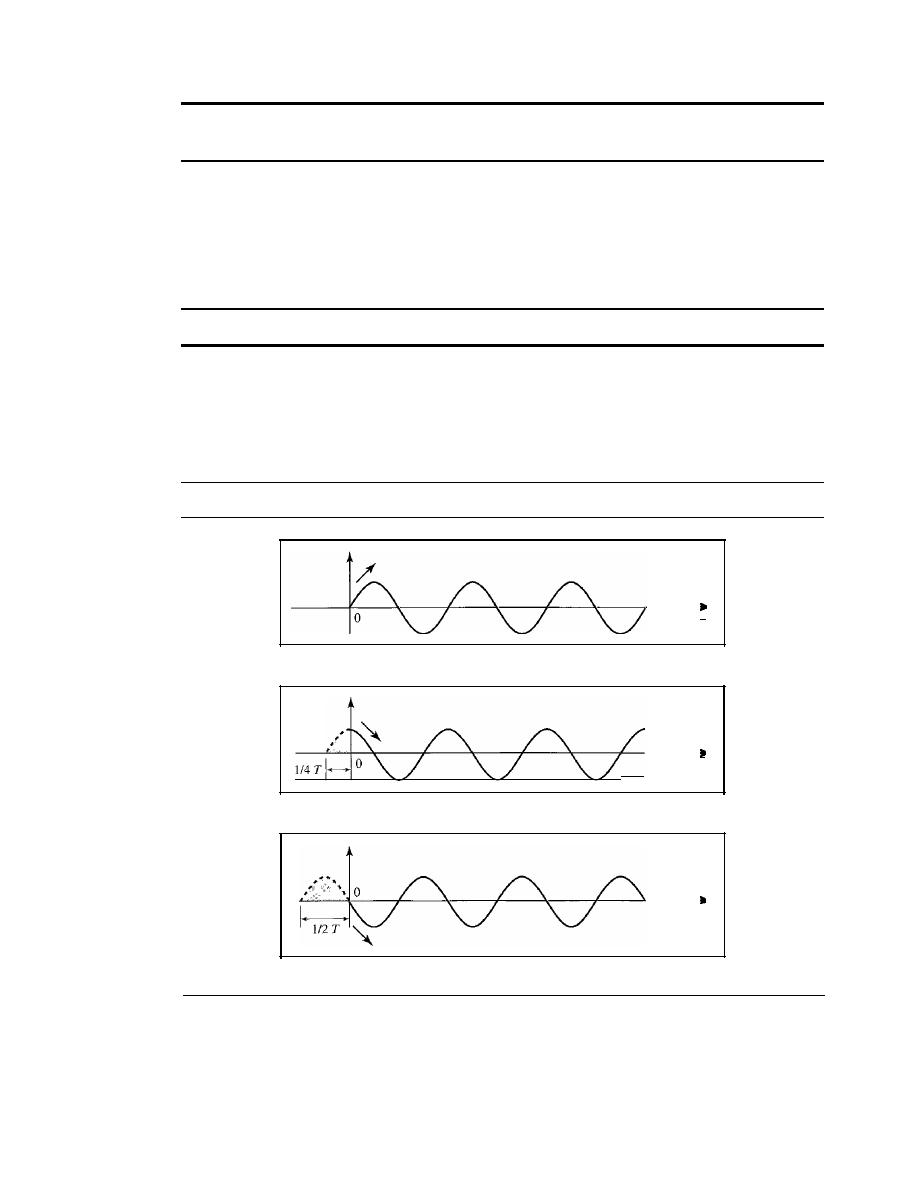
SECTION
3.2
PERiODIC ANALOG SIGNALS
63
If
a signal does not change at all, its frequency is zero.
If
a signal changes instantaneously, its frequency is infinite.
Phase
The term phase describes the position of the waveform relative to time O. If we think of
the wave as something that can be shifted backward or forward along the time axis,
phase describes the amount of that shift. It indicates the status of the first cycle.
Phase describes the position of the waveform relative to time O.
Phase is measured in degrees or radians [360° is
2n
rad; 1° is
2n/360
rad, and 1 rad
is
360/(2n)].
A phase shift of 360° corresponds to a shift of a complete period; a phase
shift of 180° corresponds
to
a shift of one-half of a period; and a phase shift of 90° cor-
responds to a shift of one-quarter of a period (see Figure 3.5).
Figure 3.5
Three sine waves with the same amplitude andfrequency, but different phases
a.
0
degrees
b. 90 degrees
c. 180 degrees
Time
Time
Time
Looking at Figure 3.5, we can say that
I.
A sine wave with a phase of 0° starts at time 0 with a zero amplitude. The
amplitude is increasing.
2. A sine wave with a phase of 90° starts at time 0 with a peak amplitude. The
amplitude is decreasing.

64
CHAPTER
3
DATA AND SIGNALS
3. A sine wave with a phase of 180° starts at time 0 with a zero amplitude. The
amplitude is decreasing.
Another way to look at the phase is in terms of shift or offset. We can say that
1. A sine wave with a phase of 0° is not shifted.
2. A sine wave with a phase of 90° is shifted to the left by
cycle. However, note
4
that the signal does not really exist before time O.
3. A sine wave with a phase of 180° is shifted to the left by
cycle. However, note
that the signal does not really exist before time O.
Example 3.6
A sine wave is offset
cycle with respect to time O. What is its phase in degrees and radians?
Solution
We know that 1 complete cycle is 360°. Therefore,
cycle is
!
360;::; 60° =60
x
tad;::;
fad;::;
1.046
rad
6
360
3
Wavelength
Wavelength is another characteristic of a signal traveling through a transmission
medium. Wavelength binds the period or the frequency of a simple sine wave to the
propagation speed of the medium (see Figure 3.6).
Figure
3.6
Wavelength and period
Wavelength
:.
':
Transmission medium
/
/
Direction of
propagation
While the frequency of a signal is independent of the medium, the wavelength
depends on both the frequency and the medium. Wavelength is a property of any type
of signal. In data communications, we often use wavelength to describe the transmis-
sion of light in an optical fiber. The wavelength is the distance a simple signal can travel
in one period.
Wavelength can be calculated if one is given the propagation speed (the speed of
light) and the period of the signal. However, since period and frequency are related to
each other, if we represent wavelength by
propagation speed by c (speed of light), and
frequency by
1,
we get
.
•
propagation speed
Wavelength
=
propagatJon speed x perJod
requency
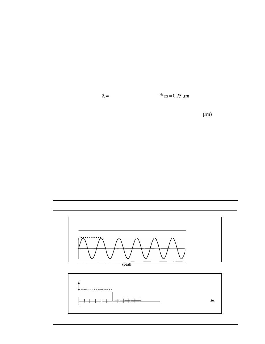
SECTION
3.2
PERIODIC ANALOG SIGNALS
6S
The propagation speed of electromagnetic signals depends on the medium and on
the frequency of the signal. For example, in a vacuum, light is propagated with a speed
of 3 x 10
8
mls. That speed is lower in air and even lower in cable.
The wavelength is normally measured in micrometers (microns) instead of meters.
For example, the wavelength of red light (frequency
=
4 x 10
14
)
in air is
8
c
3xlO
- =
=0.75 x 10
f
4x 10
14
In a coaxial or fiber-optic cable, however, the wavelength is shorter (0.5
because the
propagation speed in the cable is decreased.
Time and Frequency Domains
A sine wave is comprehensively defined by its amplitude, frequency, and phase. We
have been showing a sine wave by using what is called a
time-domain
plot. The
time-domain plot shows changes in signal amplitude with respect to time (it is an
amplitude-versus-time plot). Phase is not explicitly shown on a time-domain plot.
To show the relationship between amplitude and frequency, we can use what is
called a
frequency-domain
plot. A frequency-domain plot is concerned with only the
peak value and the frequency. Changes of amplitude during one period are not shown.
Figure 3.7 shows a signal in both the time and frequency domains.
Figure 3.7
The time-domain andfrequency-domain plots ofa sine wave
Amplitude
Frequency: 6 Hz
Peak value: 5 V
5
Time
(s)
a. A sine wave in the time domain
value: 5 V, frequency: 6 Hz)
Amplitude
Peak value: 5 V
5
-+-1
-+1-+-1
1
2
3
4
5
6
7
8
9 10 11 12 13 14
Frequency
(Hz)
b. The same sine wave in the frequency domain (peak value: 5 V, frequency: 6 Hz)
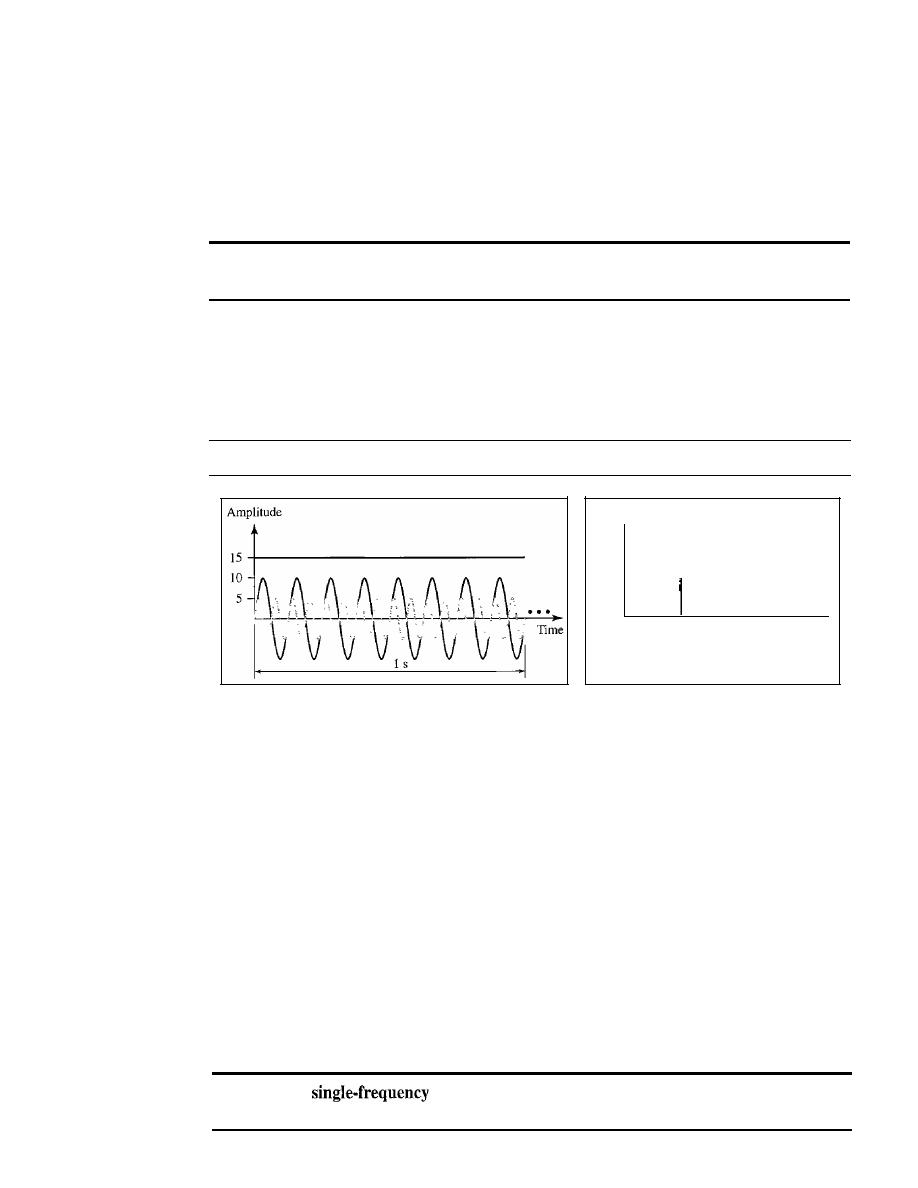
66
CHAPTER
3
DATA AND SIGNALS
It
is obvious that the frequency domain is easy to plot and conveys the information
that one can find in a time domain plot. The advantage of the frequency domain is that
we can immediately see the values of the frequency and peak amplitude. A complete
sine wave is represented by one spike. The position of the spike shows the frequency;
its height shows the peak amplitude.
A complete sine wave in the time domain can be represented
by one single spike in the frequency domain.
Example 3.7
The frequency domain is more compact and useful when we are dealing with more than one sine
wave. For example, Figure 3.8 shows three sine waves, each with different amplitude and fre-
quency. All can be represented by three spikes in the frequency domain.
Figure 3.8
The time domain and frequency domain of three sine waves
Amplitude
15 -
10 -
5-
o
8
16
Frequency
a. Time-domain representation of three sine waves with
frequencies 0, 8, and 16
b. Frequency-domain representation of
the same three signals
- - - - - - - - - - - - - - - - - - - - - - - - - - - - - - - - - - - - - - -
Composite Signals
So far, we have focused on simple sine waves. Simple sine waves have many applica-
tions in daily life. We can send a single sine wave to carry electric energy from one
place to another. For example, the power company sends a single sine wave with a fre-
quency of 60 Hz to distribute electric energy to houses and businesses. As another
example, we can use a single sine wave to send an alarm to a security center when a
burglar opens a door or window in the house. In the first case, the sine wave is carrying
energy; in the second, the sine wave is a signal of danger.
If
we had only one single sine wave to convey a conversation over the phone, it
would make no sense and carry no information. We would just hear a buzz. As we will
see in Chapters 4 and 5, we need to send a composite signal to communicate data. A
composite signal is made of many simple sine waves.
A
sine wave is not useful
in
data communications;
we need to send a composite signal, a signal made of many simple sine waves.
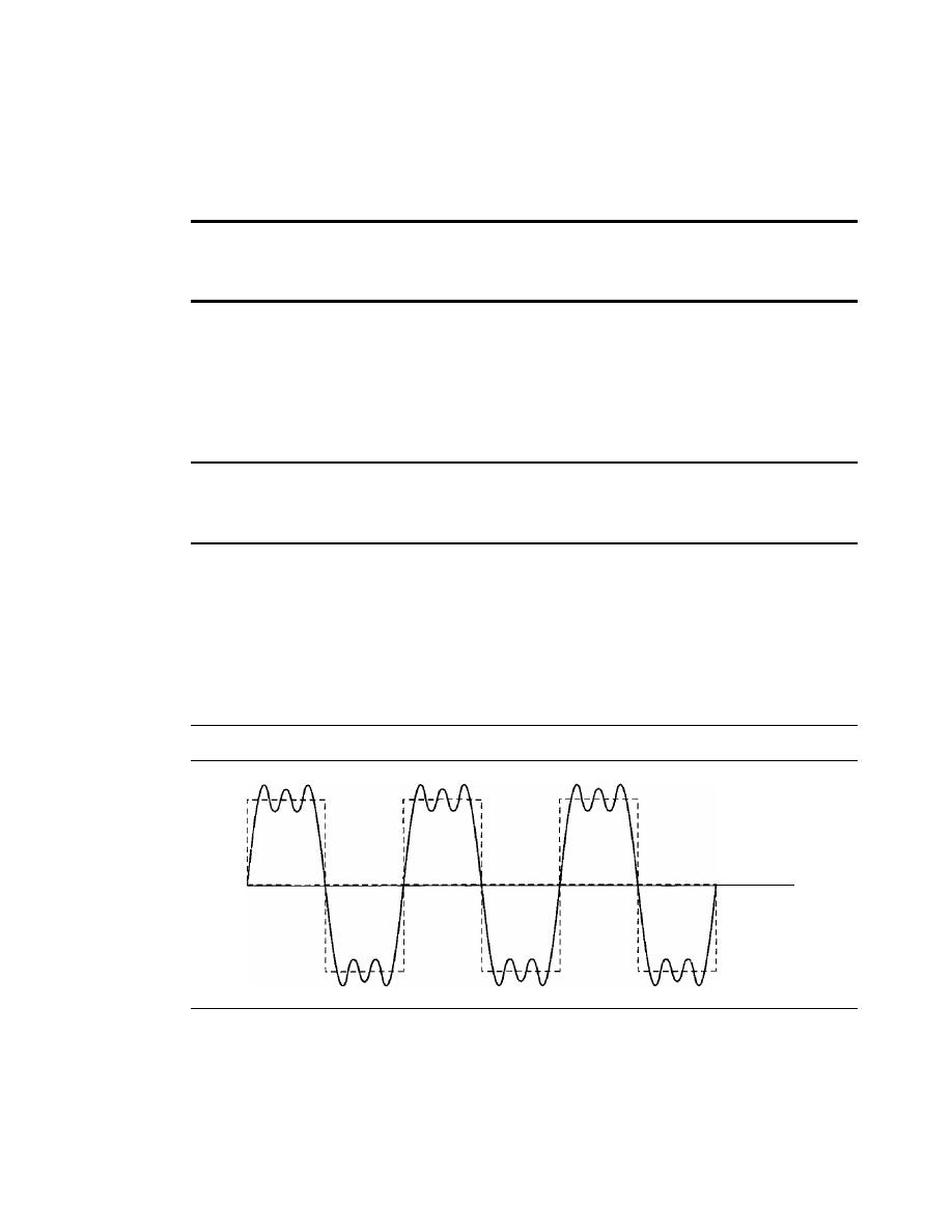
SECTION
3.2
PERIODIC ANALOG SIGNALS
67
In the early 1900s, the French mathematician Jean-Baptiste Fourier showed that
any composite signal is actually a combination of simple sine waves with different fre-
quencies, amplitudes, and phases.
Fourier analysis is discussed in Appendix C; for our
purposes, we just present the concept.
According to Fourier analysis, any composite signal is a combination of
simple sine waves with different frequencies, amplitudes, and phases.
Fourier analysis is discussed in Appendix C.
A composite signal can be periodic or nonperiodic. A periodic composite signal
can be decomposed into a series of simple sine waves with discrete frequencies-
frequencies that have integer values
(1,
2, 3, and so on). A nonperiodic composite sig-
nal can be decomposed into a combination of an infinite number of simple sine waves
with continuous frequencies, frequencies that have real values.
If
the composite signal is periodic, the decomposition gives a series of signals with
discrete frequencies; if the composite signal is nonperiodic, the decomposition
gives a combination of sine waves with continuous frequencies.
Example 3.8
Figure 3.9 shows a periodic composite signal with frequency
f
This type of signal is not typical
of those found in data communications.We can consider it to be three alarm systems, each with a
different frequency. The analysis of this signal can give us a good understanding of how to
decompose signals.
Figure 3.9
A composite periodic signal
...
Time
It
is very difficult to manually decompose this signal into a series of simple sine waves.
However, there are tools, both hardware and software, that can help us do the job. We are not con-
cerned about how
it
is done; we are only interested in the result. Figure 3.10 shows the result of
decomposing the above signal in both the time and frequency domains.
The amplitude of the sine wave with frequency
f
is almost the same as the peak amplitude of
the composite signal. The amplitude of the sine wave with frequency
3f
is one-third of that of the
first, and the amplitude of the sine wave with frequency
9f
is one-ninth of the first. The frequency
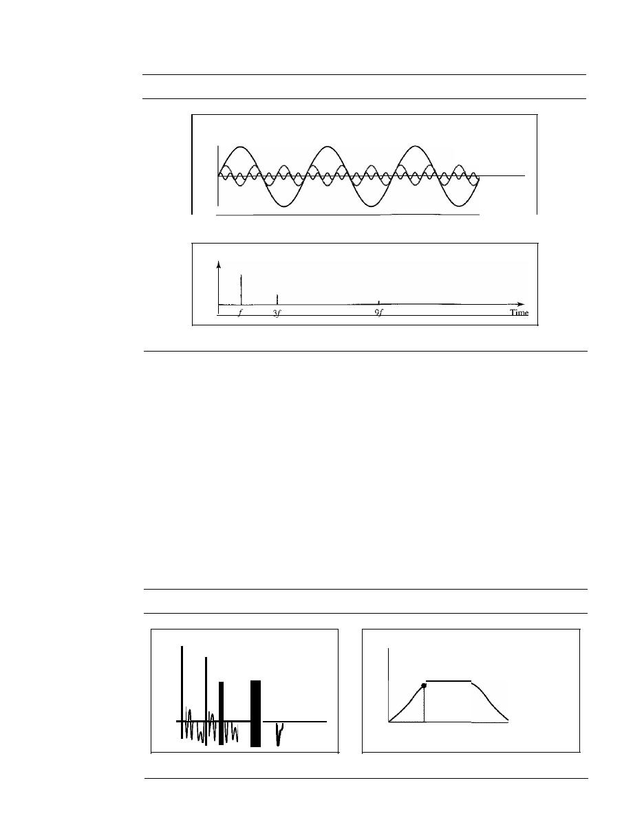
68
CHAPTER
3
DATA AND SIGNALS
Figure 3.10
Decomposition of a composite periodic signal in the time and frequency domains
Amplitude
a. Time-domain decomposition of a composite signal
-
Frequency
1
-
Frequency
31
-
Frequency
91
Time
Amplitude
b. Frequency-domain decomposition of the composite signal
of the sine wave with frequency
f
is the same as the frequency of the composite signal; it is called
the
fundamental frequency,
or first
harmonic.
The sine wave with frequency 3fhas a frequency
of 3 times the fundamental frequency; it is called the third harmonic. The third sine wave with fre-
quency 9fhas a frequency of 9 times the fundamental frequency; it is called the ninth harmonic.
Note that the frequency decomposition of the signal is discrete; it has frequenciesf,
3f,
and
9f
Because f is an integral number, 3f and 9f are also integral numbers. There are no frequencies
such as 1.2f or 2.6f The frequency domain of a periodic composite signal is always made of dis-
crete spikes.
Example 3.9
Figure 3.11 shows a nonperiodic composite signal.
It
can be the signal created by a microphone or a
telephone set when a word or two is pronounced. In this case, the composite signal cannot be peri-
odic, because that implies that we are repeating the same word or words with exactly the same tone.
Figure 3.11
The time and frequency domains of a nonperiodic signal
Amplitude
Amplitude
Amplitude for sine
wave of frequency
1
a. Time domain
,
Time
1
b. Frequency domain
4 kHz
Frequency
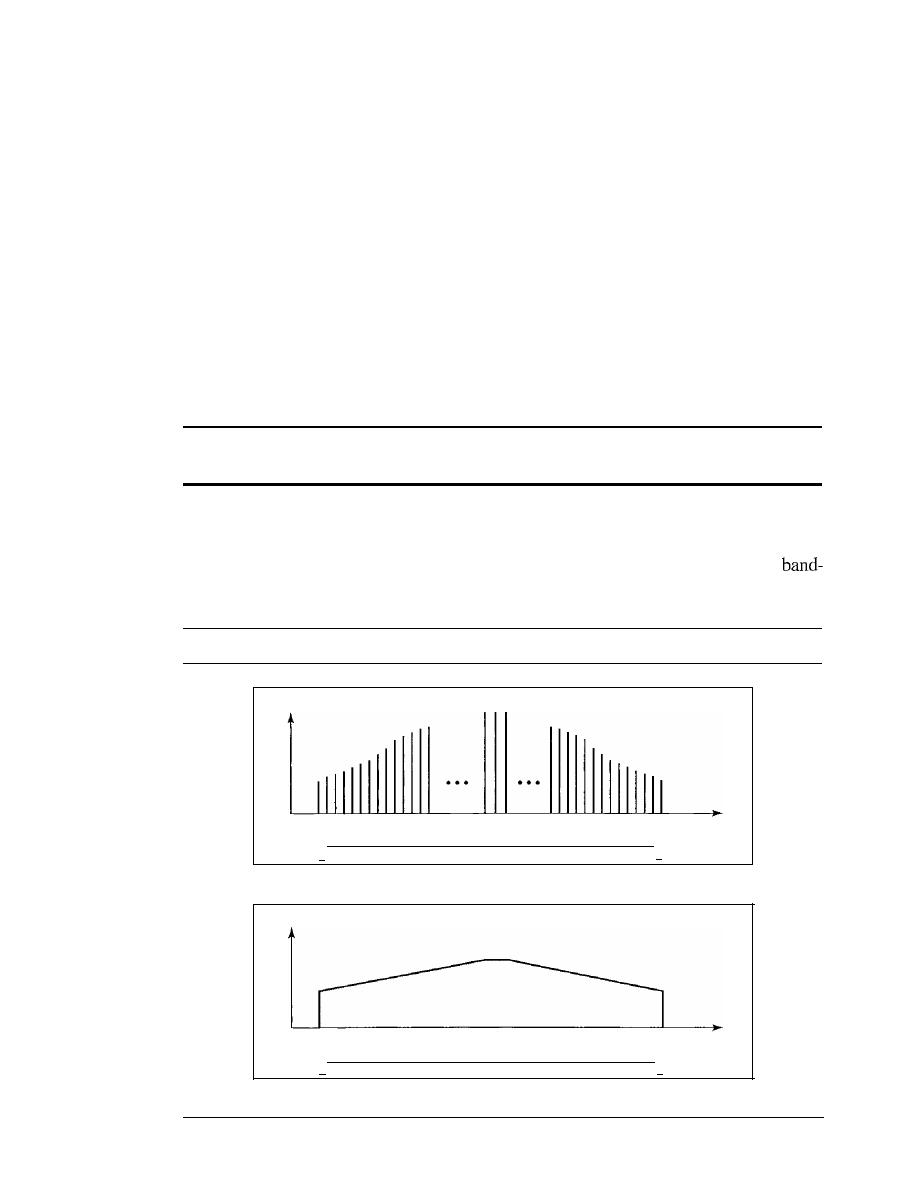
SECTION
3.2
PERIODIC ANALOG SIGNALS
69
In a time-domain representation of this composite signal, there are an infinite num-
ber of simple sine frequencies. Although the number of frequencies in a human voice is
infinite, the range is limited. A normal human being can create a continuous range of
frequencies between 0 and 4 kHz.
Note that the frequency decomposition of the signal yields a continuous curve.
There are an infinite number of frequencies between 0.0 and 4000.0 (real values). To find
the amplitude related to frequency
J,
we draw a vertical line atfto intersect the envelope
curve. The height of the vertical line is the amplitude of the corresponding frequency.
Bandwidth
The range of frequencies contained in a composite signal is its bandwidth. The band-
width is normally a difference between two numbers. For example, if a composite signal
contains frequencies between 1000 and 5000, its bandwidth is 5000 - 1000, or 4000.
The bandwidth of a composite signal is the difference between the
highest and the lowest frequencies contained in that signal.
Figure 3.12 shows the concept of bandwidth. The figure depicts two composite
signals, one periodic and the other nonperiodic. The bandwidth of the periodic signal
contains all integer frequencies between 1000 and 5000 (1000, 100 I, 1002, ...). The
width of the nonperiodic signals has the same range, but the frequencies are continuous.
Figure
3.12
The bandwidth ofperiodic and nonperiodic composite signals
Amplitude
1000
I·
Bandwidth
=
5000 - 1000
=
4000 Hz
5000
Frequency
·1
a. Bandwidth of a periodic signal
Amplitude
1000
I·
Bandwidth
=
5000 - 1000
=
4000 Hz
5000
Frequency
·1
b. Bandwidth of a nonperiodic signal

70
CHAPTER
3
DATA AND SIGNALS
Example 3.10
If a periodic signal is decomposed into five sine waves with frequencies of 100, 300, 500, 700,
and 900 Hz, what is its bandwidth? Draw the spectrum, assuming all components have a maxi-
mum amplitude of 10 V.
Solution
Letfh
be the highest frequency,
the lowest frequency, and
B
the bandwidth. Then
B
=
fh -
=
900 -
100
=
800 Hz
The spectrum has only five spikes, at 100, 300, 500, 700, and 900 Hz (see Figure 3.13).
Figure 3.13
The bandwidthfor Example 3.10
Amplitude
10+-----]
Bandwidth
=
900 - 100
=
800 Hz
100
I,
300
500
700
900
-I
Frequency
Example 3.11
A
periodic signal has a bandwidth of 20 Hz. The highest frequency is 60 Hz. What is the lowest
frequency? Draw the spectrum if the signal contains all frequencies of the same amplitude.
Solution
Letfh be the highest frequency,fz the lowest frequency, and
B
the bandwidth. Then
B
=
fh -
20
=
60 -
=
60 - 20
=
40 Hz
The spectrum contains all integer frequencies. We show this by a series of spikes (see Figure 3.14).
Figure 3.14
The bandwidth for Example 3.11
I I I
4041 42
I,
Bandwidth
=
60 - 40
=
20 Hz
585960
·1
Frequency
(Hz)
Example 3.12
A nonperiodic composite signal has a bandwidth of 200 kHz, with a middle frequency of
140 kHz and peak amplitude of 20
V.
The two extreme frequencies have an amplitude of 0. Draw
the frequency domain of the signal.
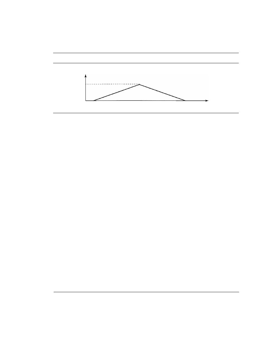
SECT/ON
3.3
DIGITAL SIGNALS
71
Solution
The lowest frequency must be at 40 kHz and the highest at 240 kHz. Figure 3.15 shows the fre-
quency domain and the bandwidth.
Figure 3.15
The bandwidth for Example 3.12
Amplitude
40 kHz
140kHz
240 kHz
Frequency
Example 3.
J
3
An
example of a nonperiodic composite signal is the signal propagated by an AM radio station, In
the United States, each AM radio station is assigned a lO-kHz bandwidth. The total bandwidth ded-
icated to AM radio ranges from 530 to 1700 kHz. We will show the rationale behind this lO-kHz
bandwidth in Chapter 5.
Example 3.
J
4
Another example of a nonperiodic composite signal is the signal propagated by an FM radio sta-
tion. In the United States, each FM radio station is assigned a 200-kHz bandwidth. The total
bandwidth dedicated to FM radio ranges from 88 to 108 MHz. We will show the rationale behind
this 200-kHz bandwidth in Chapter 5.
Example 3./5
Another example of a nonperiodic composite signal is the signal received by an old-fashioned
analog black-and-white TV. A TV screen is made up of pixels (picture elements) with each pixel
being either white or black. The screen is scanned 30 times per second. (Scanning is actually
60 times per second, but odd lines are scanned in one round and even lines in the next and then
interleaved.)
If
we assume a resolution of 525 x 700 (525 vertical lines and 700 horizontal lines),
which is a ratio of 3: 4, we have 367,500 pixels per screen. If we scan the screen 30 times per sec-
ond, this is 367,500 x 30
=
11,025,000 pixels per second. The worst-case scenario is alternating
black and white pixels. In this case, we need to represent one color by the minimum amplitude
and the other color by the maximum amplitude. We can send 2 pixels per cycle. Therefore, we
need 11,025,000/2
=
5,512,500 cycles per second, or Hz. The bandwidth needed is 5.5124 MHz.
This worst-case scenario has such a low probability of occurrence that the assumption is that we
need only 70 percent of this bandwidth, which is 3.85 MHz. Since audio and synchronization sig-
nals are also needed, a 4-MHz bandwidth has been set aside for each black and white TV chan-
nel. An analog color TV channel has a 6-MHz bandwidth.
3.3
DIGITAL SIGNALS
In addition to being represented by an analog signal, information can also be repre-
sented by a digital signal. For example, a I can be encoded as a positive voltage and a 0
as zero voltage. A digital signal can have more than two levels. In this case, we can
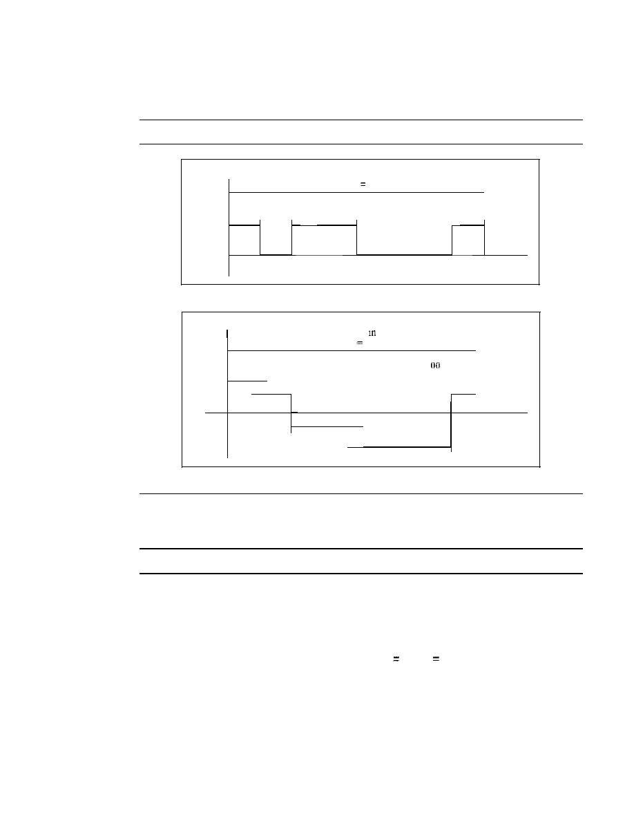
72
CHAPTER
3
DATA AND SIGNALS
send more than 1 bit for each level. Figure 3.16 shows two signals, one with two levels
and the other with four.
Figure 3.16
Two digital signals: one with two signal levels and the other with four signal levels
Amplitude
8 bits sent in
I
s,
Levell
Levell
Bit rate
8 bps
1
I
0
I
1
I
I
I
0
I
0
I
0
I
1
I
I
I
I
I
I
I
I
I
I
I
I
I
I
I
I
I
I
I
I
I
I
I
...
I
I
I
I
I
I
I
I
s
I
I
I
I
I
I
I
Tim
I
I
I
I
I
I
I
e
a.
A
digital signal with two levels
e
6 b"
"1
I
Its sent
s,
Bit rate
16 bps
II
I
10
I
01
[
01
I
00
00
[
I
10
I
I
I
I
I
I
I
I
el4
,
I
I
I
I
I
I
I
I
I
I
I
I
I
I
I
I
I
I
I
el3
[
I
I
I ...
I
I
I
[
I
I
I
I
I
s
I
I
I
I
Tim
ell
I
I
I
I
I
[
[
ell
I
I
[
I
I
I
I
[
I
I
I
I
I
Lev
Amplitude
Lev
Lev
Lev
b. A digital signal with four levels
We send 1 bit per level in part a of the figure and 2 bits per level in part b of the
figure. In general, if a signal has
L
levels, each level needs
log2L
bits.
Appendix C reviews information about exponential and logarithmic functions.
Example 3.16
A digital signal has eight levels. How many bits are needed per level? We calculate the number
of bits from the formula
Number of bits per level
log2 8
3
Each signal level is represented by 3 bits.
Example 3.17
A digital signal has nine levels. How many bits are needed per level? We calculate the number of
bits by using the formula. Each signal level is represented by 3.17 bits. However, this answer is
not realistic. The number of bits sent per level needs to be an integer as well as a power of 2. For
this example, 4 bits can represent one level.

SECTION
3.3
DIGITAL SIGNALS
73
Bit Rate
Most digital signals are nonperiodic, and thus period and frequency are not appropri-
ate characteristics. Another
term-bit rate
(instead
ofjrequency)-is
used to describe
digital signals. The
bit rate is the number of bits sent in Is, expressed in bits per
second (bps). Figure 3.16 shows the bit rate for two signals.
Example 3.18
Assume we need to download text documents at the rate of 100 pages per minute. What is the
required bit rate of the channel?
Solution
A page is an average of 24 lines with 80 characters in each line. If we assume that one character
requires 8 bits, the bit rate is
100
x
24
x
80
x
8
=
1,636,000 bps
=
1.636 Mbps
Example 3.19
A digitized voice channel, as we will see in Chapter 4, is made by digitizing a 4-kHz bandwidth
analog voice signal. We need to sample the signal at twice the highest frequency (two samples
per hertz). We assume that each sample requires 8 bits. What is the required bit rate?
Solution
The bit rate can be calculated as
2
x
4000
x
8
=
64,000 bps
=
64 kbps
Example 3.20
What is the bit rate for high-definition TV (HDTV)?
Solution
HDTV uses digital signals to broadcast high quality video signals. The HDTV Screen is normally
a ratio of 16 : 9 (in contrast to 4 : 3 for regular TV), which means the screen is wider. There are
1920 by 1080 pixels per screen, and the screen is renewed 30 times per second. Twenty-four bits
represents one color pixel. We can calculate the bit rate as
1920
x
1080
x
30
x
24
=
1,492,992,000
or
1.5 Gbps
The TV stations reduce this rate to 20 to 40 Mbps through compression.
Bit Length
We discussed the concept of the wavelength for an analog signal: the distance one cycle
occupies on the transmission medium. We can define something similar for a digital
signal: the bit length. The
bit length is the distance one bit occupies on the transmis-
sion medium.
Bit length
propagation speed x bit duration
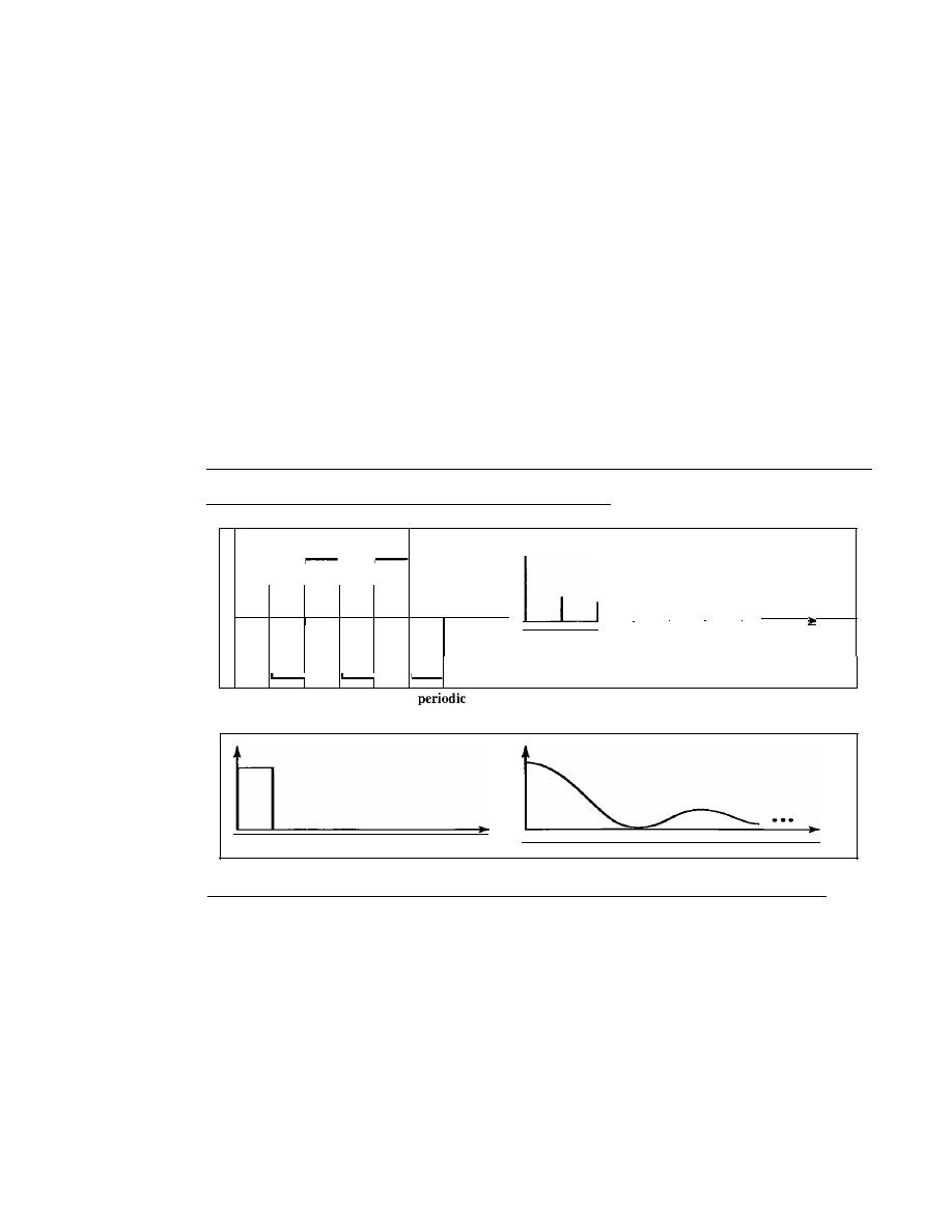
74
CHAPTER
3
DATA AND SIGNALS
Digital Signal as a Composite Analog Signal
Based on Fourier analysis, a digital signal is a composite analog signal. The bandwidth
is infinite, as you may have guessed. We can intuitively corne up with this concept when
we consider a digital signal. A digital signal, in the time domain, comprises connected
vertical and horizontal line segments. A vertical line in the time domain means a fre-
quency of infinity (sudden change in time); a horizontal line in the time domain means a
frequency of zero (no change in time). Going from a frequency of zero to a frequency of
infinity (and vice versa) implies all frequencies in between are part of the domain.
Fourier analysis can be used to decompose a digital signal. If the digital signal is
periodic, which is rare in data communications, the decomposed signal has a frequency-
domain representation with an infinite bandwidth and discrete frequencies. If the digital
signal is nonperiodic, the decomposed signal still has an infinite bandwidth, but the fre-
quencies are continuous. Figure 3.17 shows a periodic and a nonperiodic digital signal
and their bandwidths.
Figure 3.17
The time andfrequency domains ofperiodic and nonperiodic digital signals
---- - - - - - - - - - - - -
-
...
I
I
I
I
...
Time
/
3/
5f
7f
9f
Ilf
I3f
Frequency
a. Time and frequency domains of
digital signal
o
Time
Frequency
b. Time and frequency domains of nonperiodic digital signal
Note that both bandwidths are infinite, but the periodic signal has discrete frequen-
cies while the nonperiodic signal has continuous frequencies.
Transmission of Digital Signals
The previous discussion asserts that a digital signal, periodic or nonperiodic, is a com-
posite analog signal with frequencies between zero and infinity. For the remainder of
the discussion, let us consider the case of a nonperiodic digital signal, similar to the
ones we encounter in data communications. The fundamental question is, How can we
send a digital signal from point
A
to point
B?
We can transmit a digital signal by using
one of two different approaches: baseband transmission or broadband transmission
(using modulation).
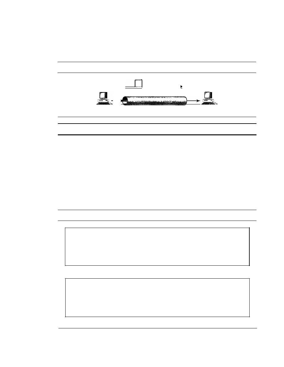
SECTION
3.3
DIGITAL SIGNALS
75
Baseband Transmission
Baseband transmission means sending a digital signal over a channel without changing
the digital signal to an analog signal. Figure 3.18 shows baseband transmission.
Figure 3.18
Baseband transmission
Digital signal
Channel
A digital signal is a composite analog signal with an infinite bandwidth.
Baseband transmission requires that we have a low-pass channel, a channel with a
bandwidth that starts from zero. This is the case if we have a dedicated medium with a
bandwidth constituting only one channel. For example, the entire bandwidth of a cable
connecting two computers is one single channel. As another example, we may connect
several computers to a bus, but not allow more than two stations to communicate at a
time. Again we have a low-pass channel, and we can use it for baseband communication.
Figure 3.19 shows two low-pass channels: one with a narrow bandwidth and the other
with a wide bandwidth. We need to remember that a low-pass channel with infinite band-
width is ideal, but we cannot have such a channel in real life. However, we can get close.
Figure 3.19
Bandwidths of two low-pass channels
o
a. Low-pass channel, wide bandwidth
o
b. Low-pass channel, narrow bandwidth
Let us study two cases of a baseband communication: a low-pass channel with a
wide bandwidth and one with a limited bandwidth.
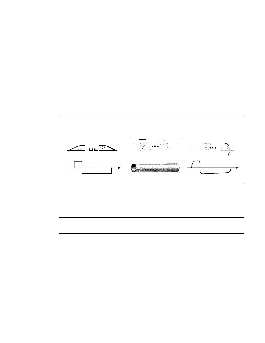
76
CHAPTER
3
DATA AND SIGNALS
Case 1: Low-Pass Channel with Wide Bandwidth
If we want to preserve the exact form of a nonperiodic digital signal with vertical seg-
ments vertical and horizontal segments horizontal, we need to send the entire spectrum,
the continuous range of frequencies between zero and infinity. This is possible if we
have a dedicated medium with an infinite bandwidth between the sender and receiver
that preserves the exact amplitude of each component of the composite signal.
Although this may be possible inside a computer (e.g., between CPU and memory), it
is not possible between two devices. Fortunately, the amplitudes of the frequencies at
the border of the bandwidth are so small that they can be ignored. This means that if we
have a medium, such as a coaxial cable or fiber optic, with a very wide bandwidth, two
stations can communicate by using digital signals with very good accuracy, as shown in
Figure 3.20. Note that!i is close to zero, andh is very high.
Figure 3.20
Baseband transmission using a dedicated medium
Input signal bandwidth
o
Input signal
Bandwidth supported
by
medium
L
Wide-bandwidth channel
Output signal bandwidth
_C
II
Output signal
Although the output signal is not an exact replica of the original signal, the data
can still be deduced from the received signal. Note that although some of the frequen-
cies are blocked by the medium, they are not critical.
Baseband transmission of a digital signal that preserves the shape of the digital signal is
possible only
if
we have a low-pass channel with an infinite or very wide bandwidth.
Example 3.21
An example of a dedicated channel where the entire bandwidth of the medium is used as one single
channel is a LAN. Almost every wired LAN today uses a dedicated channel for two stations com-
municating with each other. In a bus topology LAN with multipoint connections, only two stations
can communicate with each other at each moment in time (timesharing); the other stations need to
refrain from sending data. In a star topology LAN, the entire channel between each station and the
hub is used for communication between these two entities. We study LANs in Chapter 14.
Case 2: Low-Pass Channel with Limited Bandwidth
In a low-pass channel with limited bandwidth, we approximate the digital signal with
an analog signal. The level of approximation depends on the bandwidth available.
Rough Approximation
Let us assume that we have a digital signal of bit rate
N.
If
we
want to send analog signals to roughly simulate this signal, we need to consider the worst
case, a maximum number of changes in the digital signal. This happens when the signal
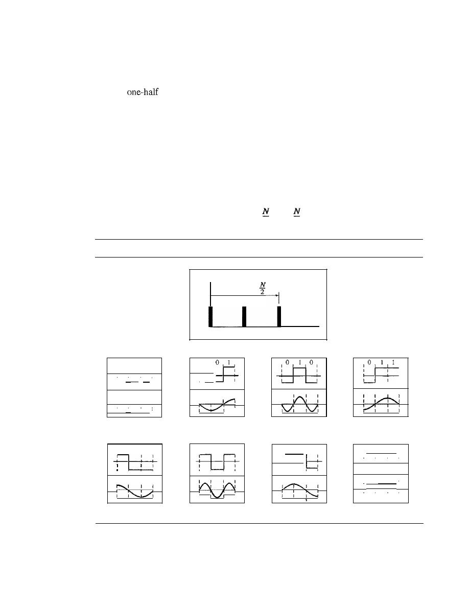
SECTION
3.3
DIGITAL SIGNALS
77
carries the sequence 01010101 ... or the sequence 10101010· ... To simulate these two
cases, we need an analog signal of frequency
f
=
N12.
Let 1 be the positive peak value and
o
be the negative peak value. We send 2 bits in each cycle; the frequency of the analog
signal is
of the bit rate, or
N12.
However, just this one frequency cannot make all
patterns; we need more components. The maximum frequency is
NI2.
As an example of
this concept, let us see how a digital signal with a 3-bit pattern can be simulated by using
analog signals. Figure 3.21 shows the idea. The two similar cases (000 and 111) are simu-
lated with a signal with frequency
f
=
0 and a phase of 180° for 000 and a phase of 0° for
111. The two worst cases (010 and 101) are simulated with an analog signal with fre-
quency
f
=
NI2
and phases of 180° and 0°. The other four cases can only be simulated with
an analog signal with
f
=
NI4
and phases of 180°, 270°, 90°, and 0°. In other words, we
need a channel that can handle frequencies 0,
N14,
and
NI2.
This rough approximation is
referred to as using the first harmonic
(NI2)
frequency. The required bandwidth is
Bandwidth
=
-
0
=
2
2
Figure 3.21
Rough approximation of a digital signal using the first harmonic for worst case
Amplitude
Bandwidth
==
o
N/4
N/2
Frequency
Digital: bit rate
N
1 ° 1
0
I
0
1
I
1
I
1
I
1
I
1
I
1
!
!
,
,
1
1
I
1
1
I
I
1
i
i
i
I
I
I
.
,
,
,
,
,
Analog:f
=
0,
p
=
180
Digital: bit rate
N
1
I
I
o
1 0 1
•
1
1
I
I
I
,
.
,
,
Analog:f=N/4, p
=
90
Digital: bit rate
N
I
0
1
I
1
:
:
,
,
,
,
I
I
I
I
I
I
I
,
,
,
.
Analog:f==N/4,p=
180
Digital: bit rate
N
I
1
I
o
1
1
I
I
I
,
,
.
,
Analog:j==
N/2, P
=
0
Digital: bit rate
N
I
I
I
1
J
I
I
I
1
1
,
,
,
,
Analog:j==N/2, p == 180
Digital: bit rate
N
1
1
I
1
I
°
I
:
,
I
1
I
,
,
I
I
j
I
J
,
,
Analog:f=N/4,p== 0
Digital: bit rate
N
I
I
,
,
,
I
I
I
I
,
,
,
,
Analog:j==N/4,
p
== 270
Digital: bit rate
N
I
1
1
I
I
I
1
i
i
I
i
I
I
I
I
I
1
I
1
,
,
,
,
I
!
1
,
I
I
I
I
I
I
i
I
I
1
I
I
,
,
,
,
Analog:
j
== 0,
p
=
0
Better Approximation
To make the shape of the analog signal look more like that
of a digital signal, we need to add more harmonics of the frequencies. We need to
increase the bandwidth. We can increase the bandwidth to
3N12, 5N12,
7
NI2,
and so on.
Figure 3.22 shows the effect of this increase for one of the worst cases, the pattern 010.
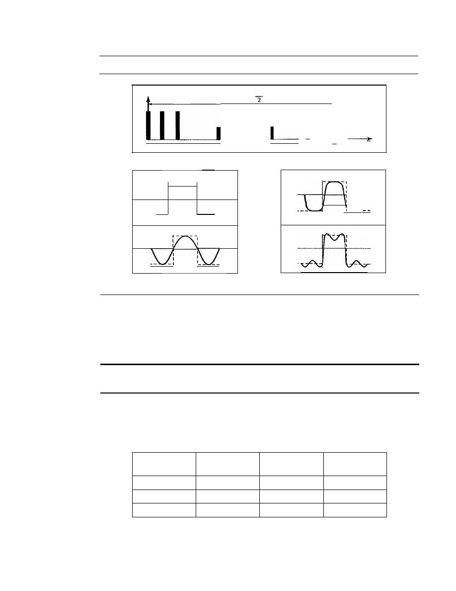
78
CHAPTER
3
DATA AND SIGNALS
Figure 3.22
Simulating a digital signal with three first harmonics
I
1
5N/4
5N12
Frequency
o
N/4 NI2
3N/4
3N12
Amplitude
5N
Bandwidth
=
Digital: bit rate
N
Analog:/=
NI2 and 3N12
0
1
I
0
I
I
I
I
I
I
I
I
I
I
I
I
I
I
I
I
I
I
I
I
I
I
U
I
I
1
Analog:!
=
N/2
Analog:!=
N12, 3N12, and 5NI2
Note that we have shown only the highest frequency for each hannonic. We use the first,
third, and fifth hannonics. The required bandwidth is now
5NJ2,
the difference between the
lowest frequency
0
and the highest frequency
5NJ2.
As we emphasized before, we need
to remember that the required bandwidth is proportional to the bit rate.
In
baseband transmission, the required bandwidth is proportional to the bit rate;
if
we need to send bits faster, we need more bandwidth.
By using this method, Table
3.2
shows how much bandwidth we need to send data
at different rates.
Table 3.2
Bandwidth requirements
Bit
Harmonic
Harmonics
Harmonics
Rate
1
1,3
1,3,5
n
=
1 kbps
B=500Hz
B= 1.5 kHz
B=2.5 kHz
n
=
10 kbps
B=5 kHz
B= 15kHz
B= 25 kHz
n
=
100 kbps
B= 50kHz
B
=
150 kHz
B= 250 kHz
Example 3.22
What is the required bandwidth of a low-pass channel if we need to send
1
Mbps
by
using base-
band transmission?
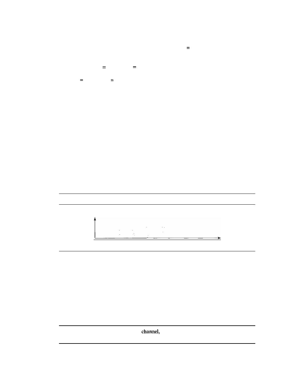
Bandpass channel
SECTION 3.3
DIGITAL SIGNALS
79
Solution
The answer depends on the accuracy desired.
a. The minimum bandwidth, a rough approximation, is
B
bit rate /2, or 500 kHz. We need
a low-pass channel with frequencies between 0 and 500 kHz.
b. A better result can be achieved by using the first and the third harmonics with the required
bandwidth
B
3
x
500 kHz
1.5 MHz.
c. Still a better result can be achieved by using the first, third, and fifth harmonics with
B
5 x 500 kHz
2.5 MHz.
Example 3.23
We have a low-pass channel with bandwidth 100 kHz. What is the maximum bit rate of this
channel?
Solution
The maximum bit rate can be achieved if we use the first harmonic. The bit rate is 2 times the
available bandwidth, or 200 kbps.
Broadband Transmission (Using Modulation)
Broadband transmission or modulation means changing the digital signal to an analog
signal for transmission. Modulation allows us to use a bandpass channel-a channel with
a bandwidth that does not start from zero. This type of channel is more available than a
low-pass channel. Figure 3.23 shows a bandpass channel.
Figure 3.23
Bandwidth of a bandpass channel
Amplitude
Frequency
Note that a low-pass channel can be considered a bandpass channel with the lower
frequency starting at zero.
Figure 3.24 shows the modulation of a digital signal. In the figure, a digital signal is
converted to a composite analog signal. We have used a single-frequency analog signal
(called a carrier); the amplitude of the carrier has been changed to look like the digital
signal. The result, however, is not a single-frequency signal; it is a composite signal, as
we will see in Chapter 5. At the receiver, the received analog signal is converted to digital,
and the result is a replica of what has been sent.
If
the available channel is a bandpass
we cannot send the digital signal directly to
the channel; we need to convert the digital signal to an analog signal before transmission.
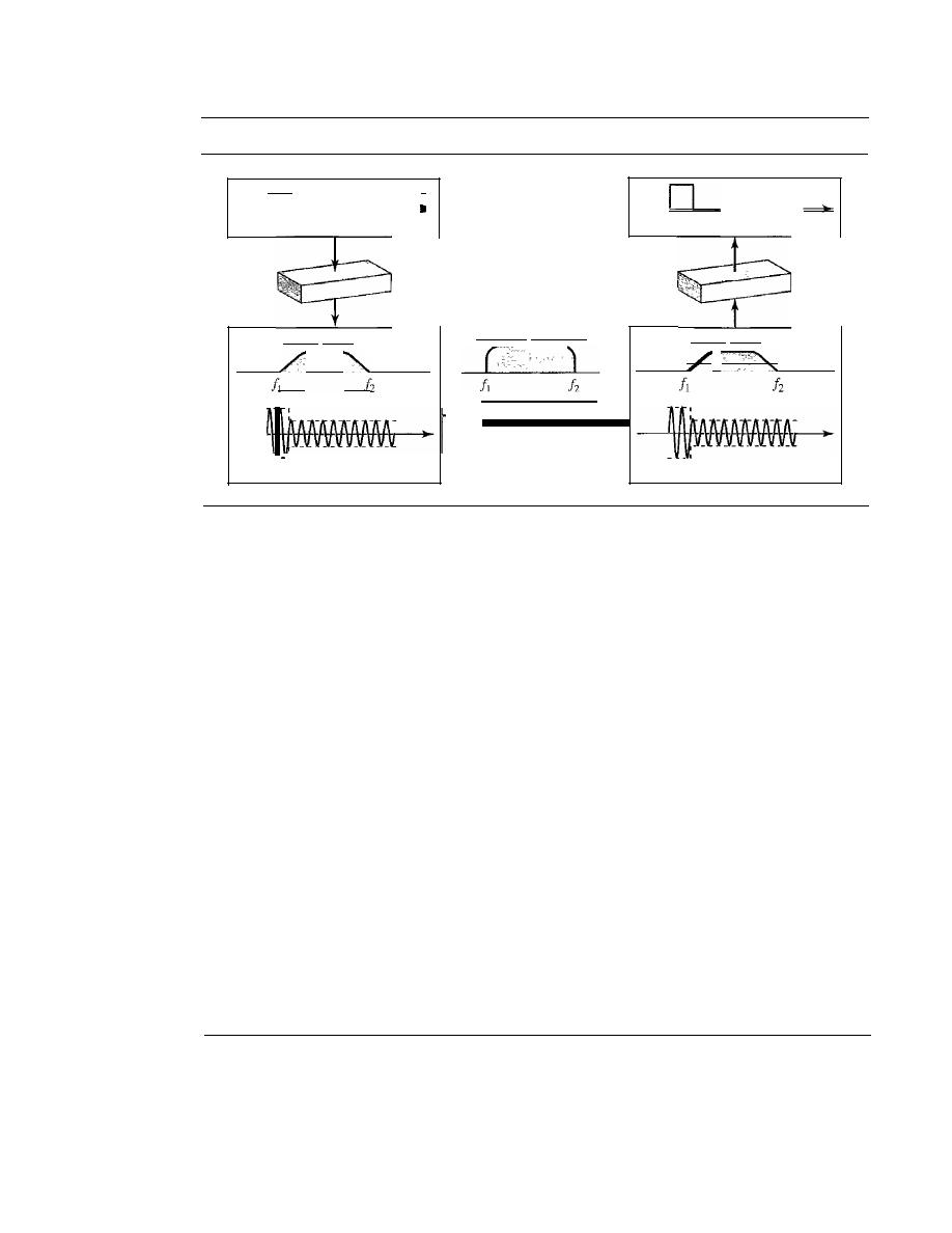
80
CHAPTER
3
DATA AND SIGNALS
Figure 3.24
Modulation of a digital signal for transmission on a bandpass channel
0
Input digi tal signal
Output digital signal
Input analog signal bandwidth
Output analog signal bandwidth
Analog/digital
con verter
Available bandwidth
DigitaUanalog
converter
-
I
Bandpass channel
Input analog signal
Input analog signal
Example 3.24
An example of broadband transmission using modulation is the sending of computer data through
a telephone subscriber line, the line connecting a resident to the central telephone office. These
lines, installed many years ago, are designed to carry voice (analog signal) with a limited band-
width (frequencies between 0 and 4 kHz). Although this channel can be used as a low-pass chan-
nel, it is normally considered a bandpass channel. One reason is that the bandwidth is so narrow
(4 kHz) that if we treat the channel as low-pass and use it for baseband transmission, the maximum
bit rate can be only 8 kbps. The solution is to consider the channel a bandpass channel, convert the
digital signal from the computer to an analog signal, and send the analog signal. We can install two
converters to change the digital signal to analog and vice versa at the receiving end. The converter,
in this case, is called a modem (modulator/demodulator), which we discuss in detail in Chapter 5.
Example 3.25
A second example is the digital cellular telephone. For better reception, digital cellular phones
convert the analog voice signal to a digital signal (see Chapter 16). Although the bandwidth allo-
cated to a company providing digital cellular phone service is very wide, we still cannot send the
digital signal without conversion. The reason is that we only have a bandpass channel available
between caller and callee. For example, if the available bandwidth is Wand we allow lOOO cou-
ples to talk simultaneously, this means the available channel is
WIlOOO,
just part of the entire
bandwidth. We need to convert the digitized voice to a composite analog signal before sending.
The digital cellular phones convert the analog audio signal to digital and then convert it again to
analog for transmission over a bandpass channel.
3.4
TRANSMISSION IMPAIRMENT
Signals travel through transmission media, which are not petfect. The impetfection causes
signal impairment. This means that the signal at the beginning of the medium is not the
same as the signal at the end of the medium. What is sent is not what is received. Three
causes of impairment are attenuation, distortion, and noise (see Figure 3.25).
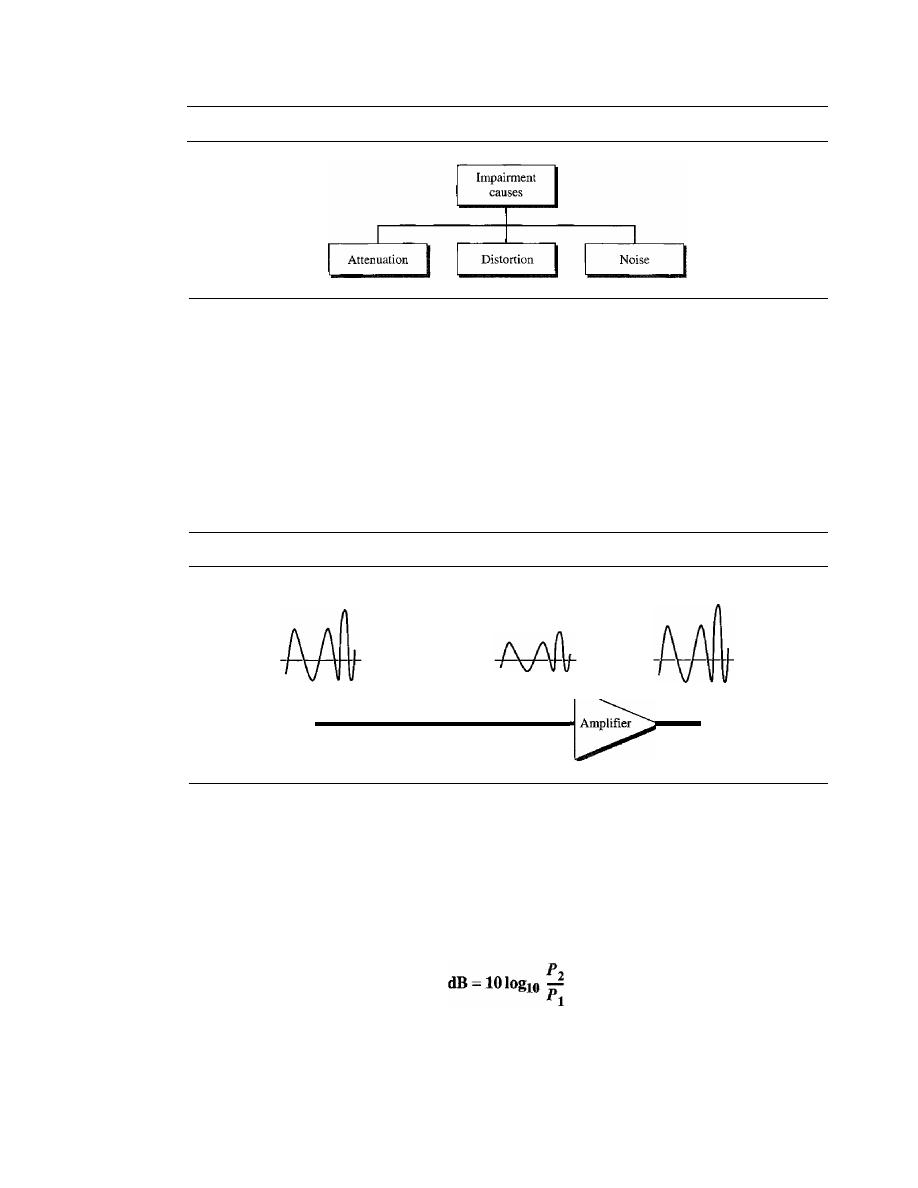
SECTION
3.4
TRANSMISSION IMPAIRMENT
81
Figure 3.25
Causes of impairment
Attenuation
Attenuation means a loss of energy. When a signal, simple or composite, travels
through a medium, it loses some of its energy in overcoming the resistance of the
medium. That is why a wire carrying electric signals gets warm, if not hot, after a
while. Some of the electrical energy in the signal is converted to heat. To compensate
for this loss, amplifiers are used to amplify the signal. Figure 3.26 shows the effect of
attenuation and amplification.
Figure 3.26
Attenuation
Original
Attenuated
Amplified
Point 1
Transmission medium
Point
2
Point 3
Decibel
To show that a signal has lost or gained strength, engineers use the unit of the decibel.
The decibel (dB) measures the relative strengths of two signals or one signal at two dif-
ferent points. Note that the decibel is negative if a signal is attenuated and positive if a
signal is amplified.
Variables
PI
and
P2
are the powers of a signal at points 1 and 2, respectively. Note that
some engineering books define the decibel in terms of voltage instead of power. In this
case, because power is proportional to the square of the voltage, the formula is dB
=
20 log
10
(V
2
IV
1).
In this text, we express dB in terms of power.
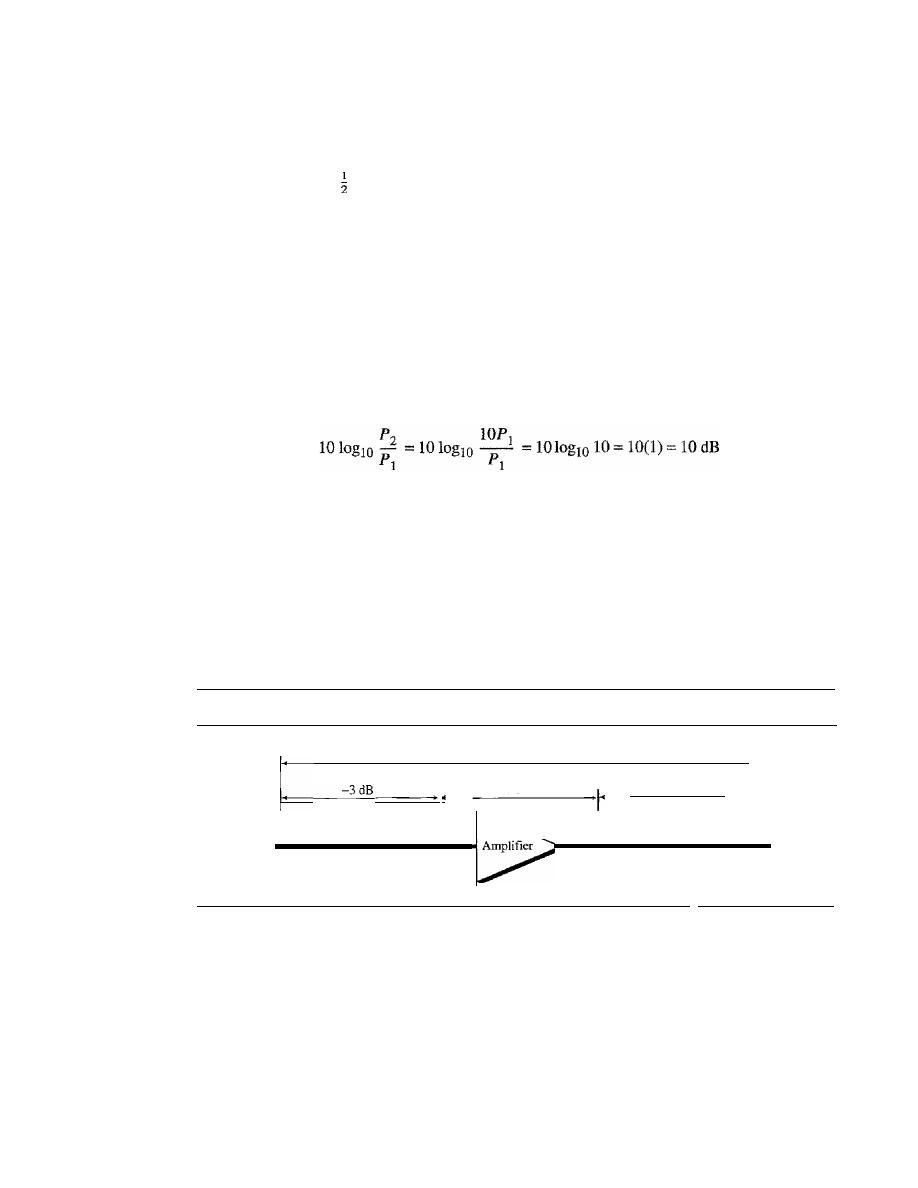
82
CHAPTER
3
DATA AND SIGNALS
Example 3.26
Suppose a signal travels through a transmission medium and its power is reduced to one-half.
This means that
P
2
=
PI'
In this case, the attenuation (loss of power) can be calculated as
P
z
0.5PI
1010glO -
= 1010gl0 - - = 10
Iogl
o
0.5 = 10(-0.3) = -3 dB
PI
PI
A loss of 3 dB (-3 dB) is equivalent to losing one-half the power.
Example 3.27
A signal travels through an amplifier, and its power is increased 10 times. This means that
P
z
=
1
OP
I'
In this case, the amplification (gain of power) can be calculated as
Example 3.28
One reason that engineers use the decibel to measure the changes in the strength of a signal is that
decibel numbers can be added (or subtracted) when we are measuring several points (cascading)
instead of just two. In Figure 3.27 a signal travels from point 1 to point 4. The signal is attenuated
by the time it reaches point 2. Between points 2 and 3, the signal is amplified. Again, between
points 3 and 4, the signal is attenuated. We can find the resultant decibel value for the signal just
by adding the decibel measurements between each set of points.
Figure 3.27
Decibels for Example 3.28
I dB
:1
7dB
-3 dB
Point 3
Transmission
Point 4
medium
Point 2
Transmission
medium
Point 1
dB
•
1
In this case, the decibel value can be calculated as
dB=-3+7-3=+1
The signal has gained in power.
Example 3.29
Sometimes the decibel is used to measure signal power in milliwatts. In this case, it is referred to
as dB
m
and is calculated as dB
m
=
10 loglO Pm' where Pm is the power in milliwatts. Calculate
the power of a signal if its dB
m
=
-30.
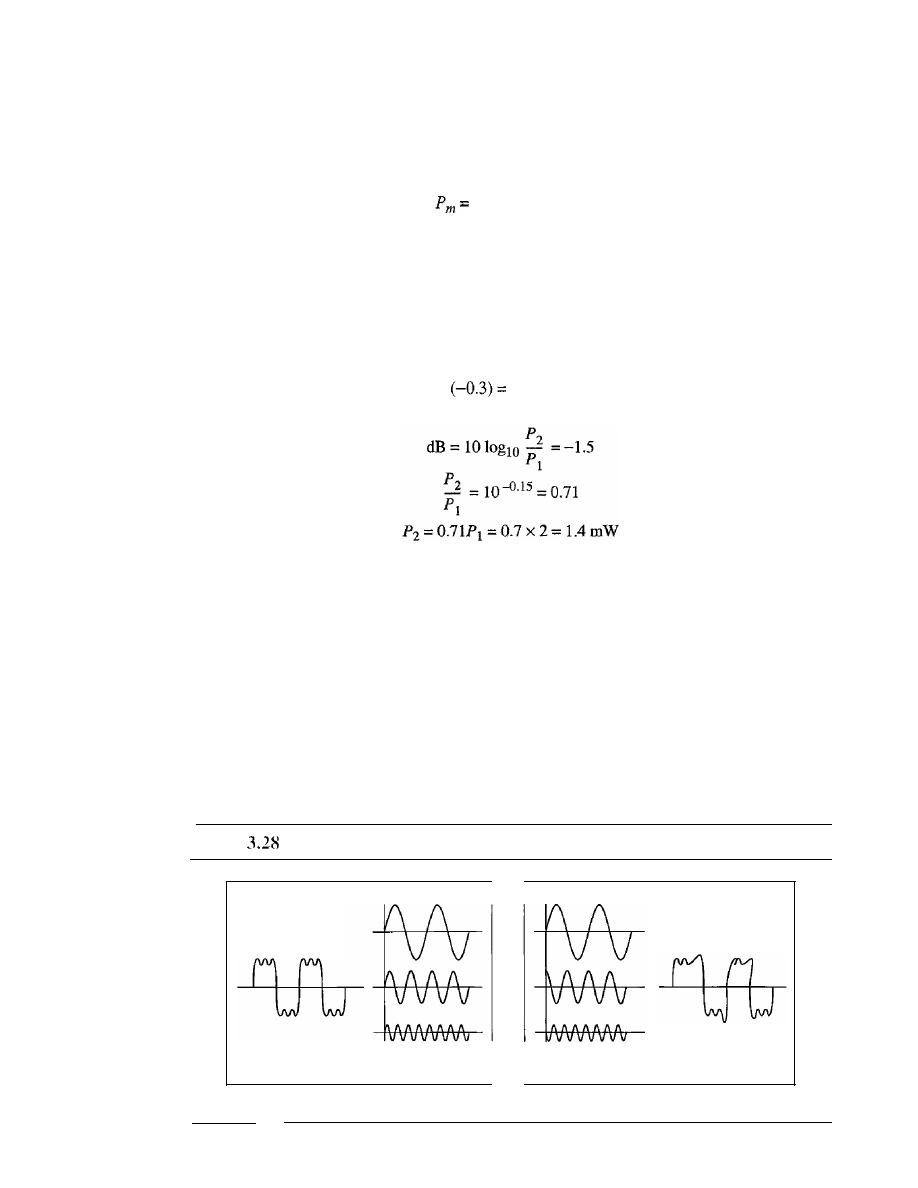
SECTION
3.4
TRANSMISSION IMPAIRMENT
83
Solution
We can calculate the power in the signal as
dB
m
=
10 log
10
Pm
=
-30
loglO
-3
Pm
=
10-
3
rnW
Example 3.30
The loss in a cable is usually defined in decibels per kilometer (dB/km).
If
the signal at the
beginning of a cable with -0.3 dBlkm has a power of 2 mW, what is the power of the signal
at 5 km?
Solution
The loss in the cable in decibels is 5 x
-1.5
dB. We can calculate the power as
Distortion
Distortion
means that the signal changes its form or shape. Distortion can occur in a
composite signal made of different frequencies. Each signal component has its own
propagation speed (see the next section) through a medium and, therefore, its own
delay in arriving at the final destination. Differences in delay may create a difference in
phase if the delay is not exactly the same as the period duration. In other words, signal
components at the receiver have phases different from what they had at the sender. The
shape of the composite signal is therefore not the same. Figure 3.28 shows the effect of
distortion on a composite signal.
Figure
Distortion
Composite signal
sent
At the sender
Components,
in phase
Composite signal
received
Components,
out of phase
At the receiver
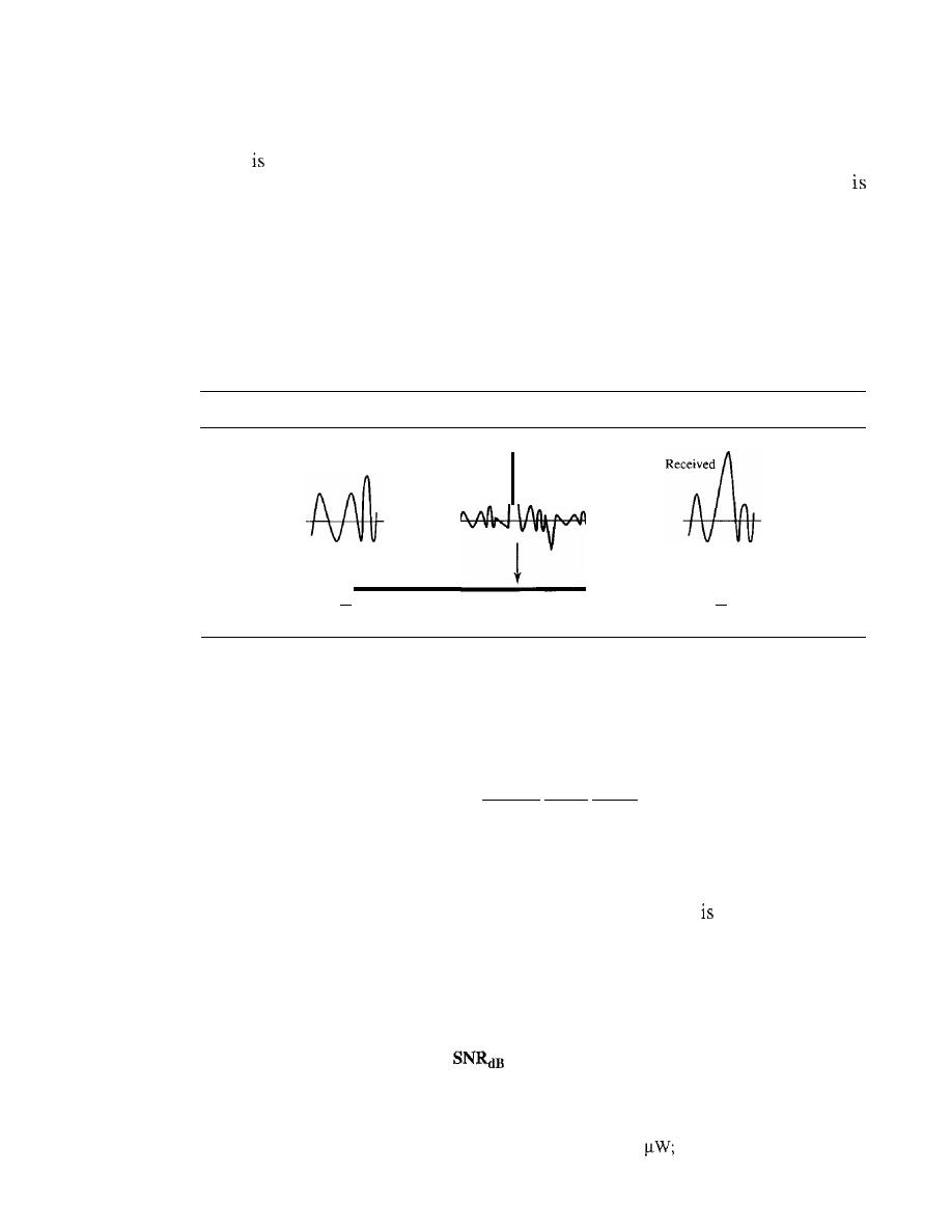
84
CHAPTER
3
DATA AND SIGNALS
Noise
Noise
another cause of impairment. Several types of noise, such as thermal noise,
induced noise, crosstalk, and impulse noise, may corrupt the signal. Thermal noise
the random motion of electrons in a wire which creates an extra signal not originally
sent by the transmitter. Induced noise comes from sources such as motors and appli-
ances. These devices act as a sending antenna, and the transmission medium acts as the
receiving antenna. Crosstalk is the effect of one wire on the other. One wire acts as a
sending antenna and the other as the receiving antenna. Impulse noise is a spike (a sig-
nal with high energy in a very short time) that comes from power lines, lightning, and so
on. Figure 3.29 shows the effect of noise on a signal. We discuss error in Chapter 10.
Figure 3.29
Noise
Transmitted
I
I
I
•
Point 1
Noise
Transmission medium
I
I
I
•
Point 2
Signal-to-Noise Ratio (SNR)
As we will see later, to find the theoretical bit rate limit, we need to know the ratio of
the signal power to the noise power. The signal-to-noise ratio is defined as
SNR
=
average signal power
average noise power
We need to consider the average signal power and the average noise power because
these may change with time. Figure 3.30 shows the idea of SNR.
SNR is actually the ratio of what is wanted (signal) to what
not wanted (noise).
A high SNR means the signal is less corrupted by noise; a low SNR means the signal is
more corrupted by noise.
Because SNR is the ratio of two powers, it is often described in decibel units,
SNR
dB,
defined as
=
lOloglo SNR
Example 3.31
The power of a signal is 10 mW and the power of the noise is 1
what are the values of SNR
and SNR
dB
?
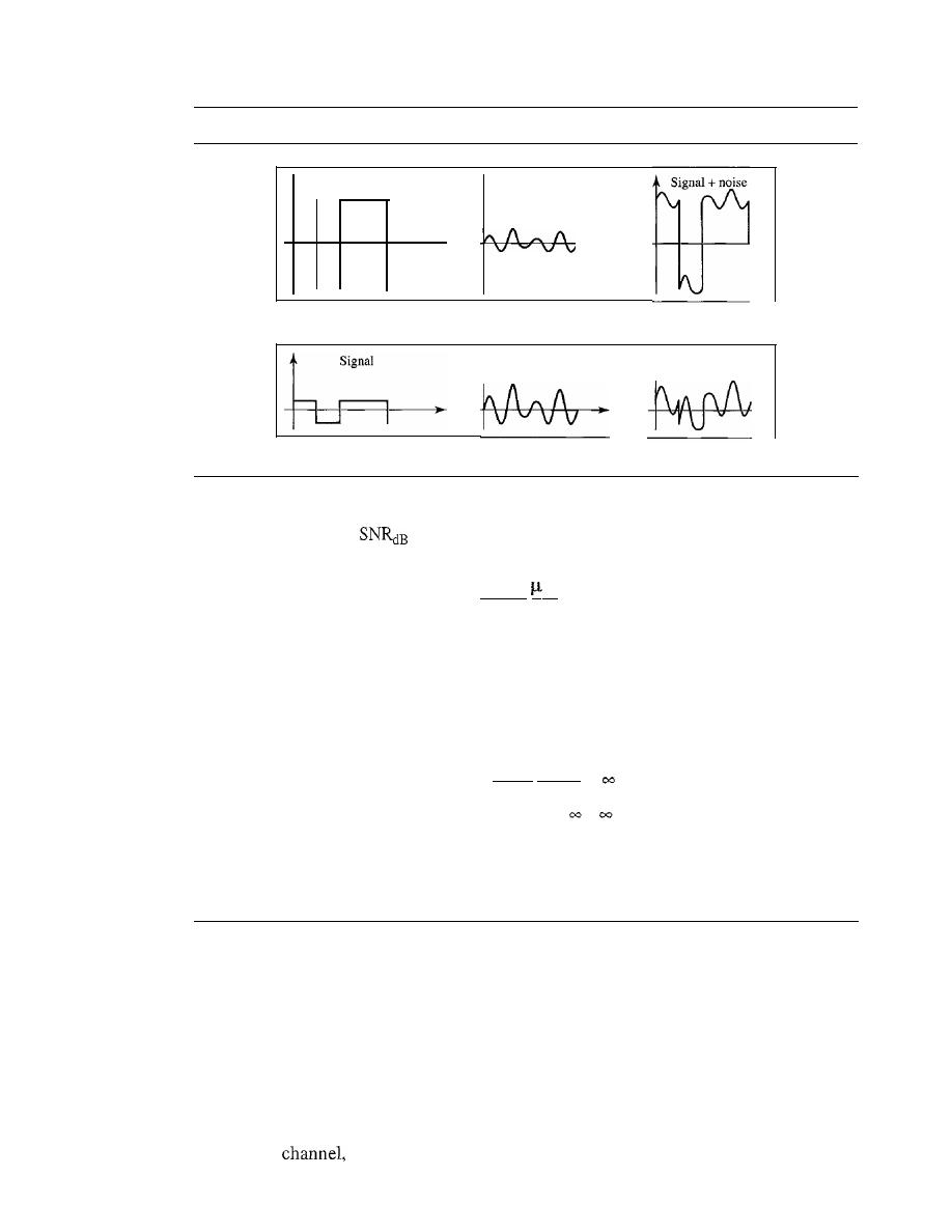
SECTION
3.5
DATA RATE LIMITS
85
Figure 3.30
Two cases of SNR: a high SNR and a low SNR
Signal
-
a. Large SNR
b. Small SNR
Noise
Noise
Signal
+
noise
Solution
The values of SNR and
can be calculated as follows:
SNR
=
10.000
W
=
10 000
ImW
'
SNR
dB
=
10 loglO 10,000
=
10 loglO 10
4
=
40
Example 3.32
The values of SNR and SNRdB for a noiseless channel are
SNR
=
signal power
=
o
SNRdB
=
10 loglO
=
We can never achieve this ratio in real life; it is an ideal.
3.5
DATA RATE LIMITS
A very important consideration in data communications is how fast we can send data, in
bits per second. over a channel. Data rate depends on three factors:
1.
The bandwidth available
2.
The level of the signals we use
3.
The quality of the channel (the level of noise)
Two theoretical formulas were developed to calculate the data rate: one by Nyquist for
a noiseless
another by Shannon for a noisy channel.

86
CHAPTER
3
DATA AND SIGNALS
Noiseless Channel: Nyquist Bit Rate
For a noiseless channel, the Nyquist bit rate formula defines the theoretical maximum
bit rate
BitRate
=
2
x
bandwidth x 10g2
L
In this formula, bandwidth is the bandwidth of the channel,
L
is the number of signal
levels used to represent data, and BitRate is the bit rate in bits per second.
According to the formula, we might think that, given a specific bandwidth, we can
have any bit rate we want by increasing the number of signa11eve1s. Although the idea
is theoretically correct, practically there is a limit. When we increase the number of sig-
nal1eve1s, we impose a burden on the receiver.
If
the number of levels in a signal is just 2,
the receiver can easily distinguish between a 0 and a 1.
If
the level of a signal is 64, the
receiver must be very sophisticated to distinguish between 64 different levels. In other
words, increasing the levels of a signal reduces the reliability of the system.
Increasing the levels of a signal may reduce the reliability of the system.
Example 3.33
Does the Nyquist theorem bit rate agree with the intuitive bit rate described in baseband
transmission?
Solution
They match when we have only two levels. We said, in baseband transmission, the bit rate is
2
times the bandwidth if we use only the first harmonic in the worst case. However, the Nyquist
formula is more general than what we derived intuitively; it can be applied to baseband transmis-
sion and modulation. Also, it can be applied when we have two or more levels of signals.
Example 3.34
Consider a noiseless channel with a bandwidth of 3000 Hz transmitting a signal with two signal
levels. The maximum bit rate can be calculated as
BitRate
=
2 x 3000 x log2 2
=
6000 bps
Example 3.35
Consider the same noiseless channel transmitting a signal with four signal levels (for each level,
we send 2 bits). The maximum bit rate can be calculated as
BitRate
=
2 x 3000
X
log2 4
=
12,000 bps
Example 3.36
We need to send 265 kbps over a noiseless channel with a bandwidth of 20 kHz. How many sig-
nallevels do we need?

SECTION
3.5
DATA RATE LIMITS
87
Solution
We can use the Nyquist formula as shown:
265,000
=
2
X
20,000
X
logz
L
log2
L
=
6.625
L
=
2
6
.
625
=
98.7 levels
Since this result is not a power of 2, we need to either increase the number of levels or reduce
the bit rate. If we have 128 levels, the bit rate is 280 kbps. If we have 64 levels, the bit rate is
240 kbps.
Noisy Channel: Shannon Capacity
In reality, we cannot have a noiseless channel; the channel is always noisy. In 1944,
Claude Shannon introduced a formula, called the Shannon capacity, to determine the
theoretical highest data rate for a noisy channel:
Capacity
=
bandwidth
X
log2 (1
+
SNR)
In this formula, bandwidth is the bandwidth of the channel, SNR is the signal-to-
noise ratio, and capacity is the capacity of the channel in bits per second. Note that in the
Shannon formula there is no indication of the signal level, which means that no matter
how many levels we have, we cannot achieve a data rate higher than the capacity of the
channel. In other words, the formula defines a characteristic of the channel, not the method
of transmission.
Example 3.37
Consider an extremely noisy channel in which the value of the signal-to-noise ratio is almost
zero. In other words, the noise is so strong that the signal is faint. For this channel the capacity C
is calculated as
C
=
B
log2
(1
+
SNR)
=
B
10g
z
(l
+
0)
=
B
log2 1
B
x
0
0
This means that the capacity of this channel is zero regardless of the bandwidth. In other
words, we cannot receive any data through this channel.
Example 3.38
We can calculate the theoretical highest bit rate of a regular telephone line.
A
telephone line nor-
mally has a bandwidth of 3000 Hz (300 to 3300 Hz) assigned for data communications. The sig-
nal-to-noise ratio is usually 3162. For this channel the capacity is calculated as
C
=
B
log2 (1
+
SNR)
=
3000 log2
(l
+
3162)
=
3000 log2 3163
3000
x
11.62
34,860 bps
This means that the highest bit rate for a telephone line is 34.860 kbps. If we want to send
data faster than this, we can either increase the bandwidth of the line or improve the signal-to-
noise ratio.

88
CHAPTER
3
DATA AND SIGNALS
Example 3.39
The signal-to-noise ratio is often given in decibels. Assume that
=
36 and the channel
bandwidth is 2 MHz. The theoretical channel capacity can be calculated as
SNR
dB
=
10
loglO
SNR
SNR
=
10
3.6
=
3981
C
=
B
log2
(1+
SNR)
= 2
X
10
6
X
log2 3982
=
24 Mbps
Example 3.40
For practical purposes, when the SNR is very high, we can assume that SNR
+
I is almost the
same as SNR. In these cases, the theoretical channel capacity can be simplified to
SNR
dB
C=BX
- - =
3
For example, we can calculate the theoretical capacity of the previous example as
36
C= 2 MHz X -
=24 Mbps
3
Using
Both Limits
In practice, we need to use both methods to find the limits and signal levels. Let us show
this with an example.
Example 3.41
We have a channel with a I-MHz bandwidth. The SNR for this channel is 63. What are the appro-
priate bit rate and signal level?
Solution
First, we use the Shannon formula to find the upper limit.
C
=
B
log2
(l
+
SNR)
=
10
6
log2 (1
+
63)
=
10
6
10g2 64
=
6 Mbps
The Shannon formula gives us 6 Mbps, the upper limit. For better performance we choose
something lower, 4 Mbps, for example. Then we use the Nyquist formula to find the number of
signal levels.
4Mbps=2x 1
MHz
x
log
2
L
L=4
The Shannon capacity gives us the upper limit;
the Nyquist formula tells us how many signal levels we need.

SECTION
3.6
PERFORMANCE
89
3.6
PERFORMANCE
Up to now, we have discussed the tools of transmitting data (signals) over a network
and how the data behave. One important issue in networking is the performance of the
network-how good is it? We discuss quality of service, an overall measurement of
network performance, in greater detail in Chapter 24. In this section, we introduce
terms that we need for future chapters.
Bandwidth
One characteristic that measures network performance is bandwidth. However, the term
can be used in two different contexts with two different measuring values: bandwidth in
hertz and bandwidth in bits per second.
Bandwidth in Hertz
We have discussed this concept. Bandwidth in hertz is the range of frequencies con-
tained in a composite signal or the range of frequencies a channel can pass. For exam-
ple, we can say the bandwidth of a subscriber telephone line is 4 kHz.
Bandwidth in Bits per Seconds
The term
bandwidth can also refer to the number of bits per second that a channel, a
link, or even a network can transmit. For example, one can say the bandwidth of a Fast
Ethernet network (or the links in this network) is a maximum of
100 Mbps. This means
that this network can send
100 Mbps.
Relationship
There is an explicit relationship between the bandwidth in hertz and bandwidth in bits
per seconds. Basically, an increase in bandwidth in hertz means an increase in bandwidth
in bits per second. The relationship depends on whether we have baseband transmission
or transmission with modulation. We discuss this relationship in Chapters
4 and 5.
In networking, we use the term bandwidth
in
two contexts.
o
The first,
bandwidth in hertz, refers to the range of frequencies in a composite
signal or the range of frequencies that a channel can pass.
o
The second,
bandwidth in bits per second, refers to the speed of bit transmis-
sion in a channel or link.
Example 3.42
The bandwidth of a subscriber line is 4 kHz for voice or data. The bandwidth of this line for data trans-
mission can be up to 56,000 bps using a sophisticated modem to change the digital signal to analog.
Example 3.43
If the telephone company improves the quality of the line and increases the bandwidth to 8 kHz,
we can send 112,000 bps by using the same technology as mentioned in Example 3.42.

90
CHAPTER
3
DATA AND SIGNALS
Throughput
The
throughput
is a measure of how fast we can actually send data through a network.
Although, at first glance, bandwidth in bits per second and throughput seem the
they are different. A link may have a bandwidth of B bps, but we can only send T bps
through this link with
T
always less than
B.
In other words, the bandwidth is a potential
measurement of a link; the throughput is an actual measurement of how fast we can
send data. For example, we may have a link with a bandwidth of
1
but the
devices connected to the end of the link may handle only 200 kbps. This means that we
cannot send more than 200 kbps through this link.
Imagine a highway designed to transmit 1000 cars per minute from one point
to another. However, if there is congestion on the road, this figure may be reduced to
100 cars per minute. The bandwidth is 1000 cars per minute; the throughput is 100 cars
per minute.
Example 3.44
A network with bandwidth of 10 Mbps can pass only an average of
frames per minute
with each frame carrying an average of 10,000 bits. What is the throughput of this network?
Solution
We can calculate the throughput as
Throughput
=
12,000 x 10,000
=
2 Mbps
60
The throughput is almost one-fifth of the bandwidth in this case.
Latency (Delay)
The latency or delay defines how long it takes for an entire message to completely
arrive at the destination from the time the first bit is sent out from the source. We can
say that latency is made of four components:
propagation time, transmission time,
queuing time
and
processing delay.
Latency
=
propagation time
+
transmission time
+
queuing time
+
processing delay
Propagation Time
Propagation time measures the time required for a bit to travel from the source to the
destination. The propagation time is calculated by dividing the distance by the propaga-
tion speed.
Propagation time
=
Propagation speed
The propagation speed of electromagnetic signals depends on the medium and on
the frequency of the signaL For example, in a vacuum, light is propagated with a speed
of 3 x 10
8
mfs. It is lower in air; it is much lower in cable.

SECTION
3.6
PERFORMANCE
91
Example 3.45
What is the propagation time if the distance between the two points is 12,000 km? Assume the
propagation speed to be 2.4 x 10
8
mls in cable.
Solution
We can calculate the propagation time as
. .
12000
x
1000
Propagation
=
'
=
50 ms
2.4
x
10
8
The example shows that a bit can go over the Atlantic Ocean in only 50 ms if there is a direct
cable between the source and the destination.
Tra/lsmissio/l
Time
In data communications we don't send just 1 bit, we send a message. The first bit may
take a time equal to the propagation time to reach its destination; the last bit also may
take the same amount of time. However, there is a time between the first bit leaving the
sender and the last bit arriving at the receiver. The first bit leaves earlier and arrives ear-
lier; the last bit leaves later and arrives later. The time required for transmission of a
message depends on the size of the message and the bandwidth of the channel.
Transmission time
=
Message size
Bandwidth
Example 3.46
What are the propagation time and the transmission time for a 2.5-kbyte message (an e-mail) if
the bandwidth of the network is 1 Gbps? Assume that the distance between the sender and the
receiver is 12,000 km and that light travels at 2.4
x
10
8
mls.
Solution
We can calculate the propagation and transmission time as
. .
12000
x
1000
PropagatIon Hme
=
x
10
8
=
50 ms
T
. . .
2500
x
8
0 020
ranSIlllSSlOn
=
9
=.
ms
10
Note that in this case, because the message is short and the bandwidth is high, the
dominant factor is the propagation time, not the transmission time. The transmission
time can be ignored.
Example 3.47
What are the propagation time and the transmission time for a 5-Mbyte message (an image) if the
bandwidth of the network is 1 Mbps? Assume that the distance between the sender and the
receiver is 12,000 km and that light travels at 2.4 x 10
8
mls.
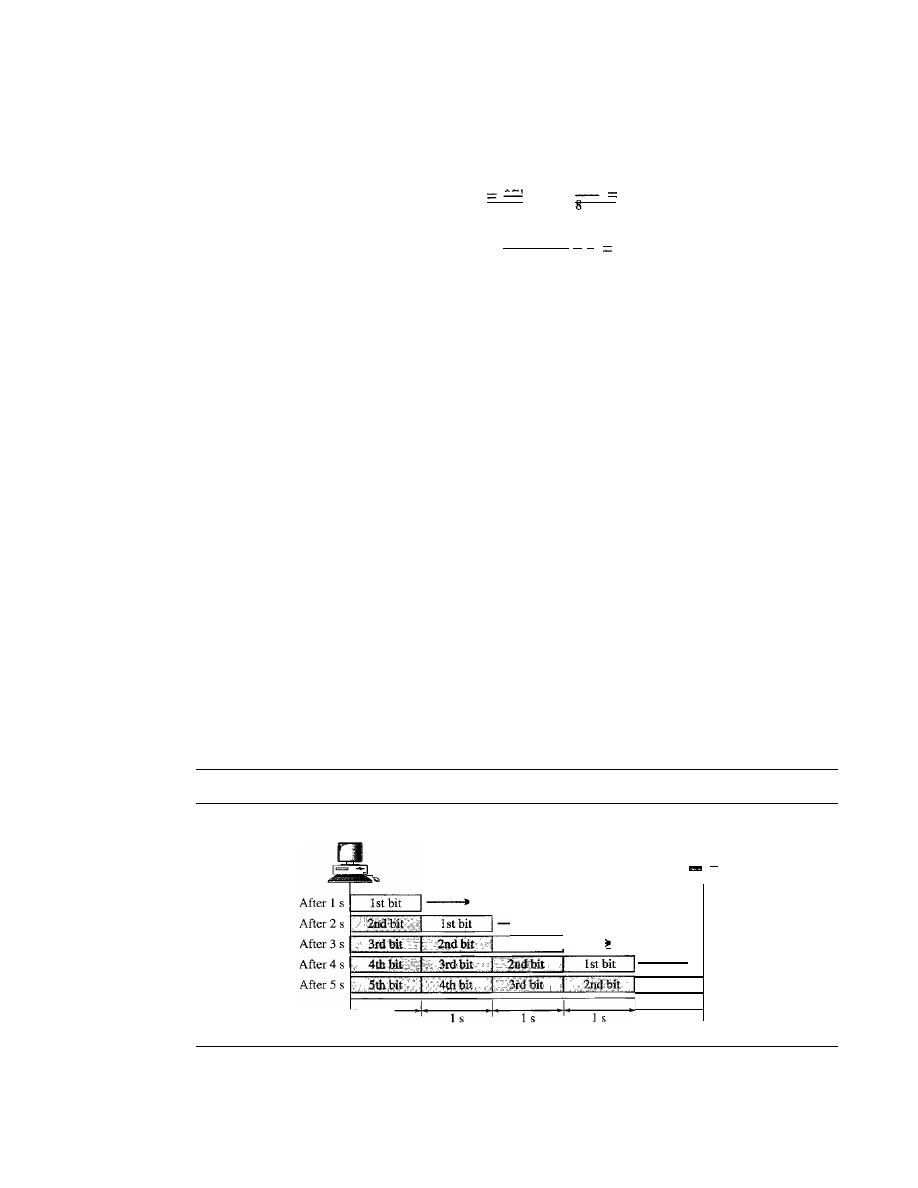
92
CHAPTER
3
DATA AND SIGNALS
Solution
We can calculate the propagation and transmission times as
. ,
12 000
X
1000
PropagatIon tIme
50
ms
2.4x
10
T
. .
.
5,000,000
x
8
40
ranSffilSSlOn
tIme::::
6
S
10
Note that in this case, because the message is very long and the bandwidth is not very
high, the dominant factor is the transmission time, not the propagation time. The propa-
gation time can be ignored.
Queuing Time
The third component in latency is the queuing time, the time needed for each interme-
diate or end device to hold the message before it can be processed. The queuing time is
not a fixed factor; it changes with the load imposed on the network. When there is
heavy traffic on the network, the queuing time increases. An intermediate device, such
as a router, queues the arrived messages and processes them one by one. If there are
many messages, each message will have to wait.
Bandwidth-Delay Product
Bandwidth and delay are two performance metrics of a link. However, as we will see in
this chapter and future chapters, what is very important in data communications is the
product of the two, the bandwidth-delay product. Let us elaborate on this issue, using
two hypothetical cases as examples.
o
Case
1.
Figure 3.31 shows case
1.
Figure 3.31
Filling the link with bits for case 1
Sender
Receiver
1
s
Bandwidth: 1 bps
Delay: 5 s
Bandwidth
x
delay
=
5 bits
1st bit
...
1st bit
1
s
Let
US
assume that we have a link with a bandwidth of 1 bps (unrealistic, but good
for demonstration purposes). We also assume that the delay of the link is 5 s (also
unrealistic). We want to see what the bandwidth-delay product means in this case.
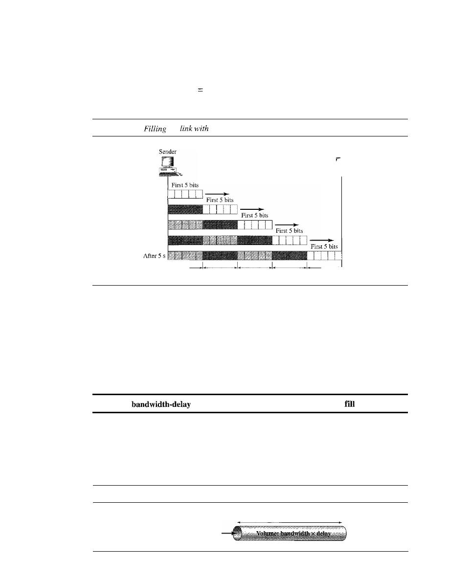
SECTION
3.6
PERFORMANCE
93
Looking at figure, we can say that this product 1 x 5 is the maximum number of
bits that can fill the link. There can be no more than 5 bits at any time on the link.
o
Case 2. Now assume we have a bandwidth of 4 bps. Figure 3.32 shows that there
can be maximum 4 x 5
20 bits on the line. The reason is that, at each second,
there are 4 bits on the line; the duration of each bit is 0.25 s.
Figure 3.32
the
bits in case 2
Bandwidth: 4 bps
Delay: 5 s
Bandwidth
x
delay
=
20 bits
After
1
s
After 2 s
After 4 s
1
s
1
s
1
s
1
s
1
s
Receiver
The above two cases show that the product of bandwidth and delay is the number of
bits that can fill the link. This measurement is important if we need to send data in bursts
and wait for the acknowledgment of each burst before sending the next one. To use the
maximum capability of the link, we need to make the size of our burst 2 times the product
of bandwidth and delay; we need to fill up the full-duplex channel (two directions). The
sender should send a burst of data of (2 x bandwidth x delay) bits. The sender then waits
for receiver acknowledgment for part of the burst before sending another burst. The
amount 2 x bandwidth x delay is the number of bits that can be in transition at any time.
The
product defines the number of bits that can
the link.
Example 3.48
We can think about the link between two points as a pipe. The cross section of the pipe represents
the bandwidth, and the length of the pipe represents the delay. We can say the volume of the pipe
defines the bandwidth-delay product, as shown in Figure 3.33.
Figure 3.33
Concept of bandwidth-delay product
Length: delay
Cross section: bandwidth

94
CHAPTER
3
DATA AND SIGNALS
Jitter
Another performance issue that is related to delay is jitter. We can roughly say that jitter
is a problem if different packets of data encounter different delays and the application
using the data at the receiver site is time-sensitive (audio and video data, for example).
If
the delay for the first packet is 20 ms, for the second is 45 ms, and for the third is
40 ms, then the real-time application that uses the packets endures jitter. We discuss jitter
in greater detail in Chapter 29.
3.7
RECOMMENDED READING
For more details about subjects discussed in this chapter, we recommend the following
books. The items in brackets [...] refer to the reference list at the end of the text.
Books
Data and signals are elegantly discussed in Chapters 1 to 6 of [Pea92]. [CouOl] gives
an excellent coverage about signals in Chapter 2. More advanced materials can be
found in [Ber96]. [Hsu03] gives a good mathematical approach to signaling. Complete
coverage of Fourier Analysis can be found in [Spi74]. Data and signals are discussed in
Chapter 3 of [Sta04] and Section 2.1 of [Tan03].
3.8
KEY TERMS
analog
analog data
analog signal
attenuation
bandpass channel
bandwidth
baseband transmission
bit rate
bits per second (bps)
broadband transmission
composite signal
cycle
decibel (dB)
digital
digital data
digital signal
distortion
Fourier analysis
frequency
frequency-domain
fundamental frequency
harmonic
Hertz (Hz)
jitter
low-pass channel
noise
nonperiodic signal
Nyquist bit rate
peak amplitude
period
periodic signal
phase
processing delay
propagation speed

propagation time
queuing time
Shannon capacity
signal
signal-to-noise ratio (SNR)
SECTION
3.9
SUMMARY
95
sine wave
throughput
time-domain
transmission time
wavelength
3.9
SUMMARY
o
Data must be transformed to electromagnetic signals to be transmitted.
o
Data can be analog or digital. Analog data are continuous and take continuous
values. Digital data have discrete states and take discrete values.
o
Signals can be analog or digital. Analog signals can have an infinite number of
values in a range; digital ,signals can have only a limited number of values.
o
In data communications, we commonly use periodic analog signals and nonperi-
odic digital signals.
o
Frequency and period are the inverse of each other.
o
Frequency is the rate of change with respect to time.
o
Phase describes the position of the waveform relative to time O.
o
A complete sine wave in the time domain can be represented by one single spike in
the frequency domain.
o
A single-frequency sine wave is not useful in data communications; we need to
send a composite signal, a signal made of many simple sine waves.
o
According to Fourier analysis, any composite signal is a combination of simple
sine waves with different frequencies, amplitudes, and phases.
o
The bandwidth of a composite signal is the difference between the highest and the
lowest frequencies contained in that signal.
o
A digital signal is a composite analog signal with an infinite bandwidth.
o
Baseband transmission of a digital signal that preserves the shape of the digital
signal is possible only if we have a low-pass channel with an infinite or very wide
bandwidth.
o
If
the available channel is a bandpass channel, we cannot send a digital signal
directly to the channel; we need to convert the digital signal to an analog signal
before transmission.
o
For a noiseless channel, the Nyquist bit rate formula defines the theoretical maxi-
mum bit rate. For a noisy channel, we need to use the Shannon capacity to find the
maximum bit rate.
o
Attenuation, distortion, and noise can impair a signal.
o
Attenuation is the loss of a signal's energy due to the resistance of the medium.
o
Distortion is the alteration of a signal due to the differing propagation speeds of
each of the frequencies that make up a signal.
o
Noise is the external energy that corrupts a signal.
o
The bandwidth-delay product defines the number of bits that can fill the link.

96
CHAPTER
3
DATA AND SIGNALS
3.10
PRACTICE SET
Review Questions
1. What is the relationship between period and frequency?
2. What does the amplitude of a signal measure? What does the frequency of a signal
measure? What does the phase of a signal measure?
3.
How can a composite signal be decomposed into its individual frequencies?
4.
Name three types of transmission impairment.
5. Distinguish between baseband transmission and broadband transmission.
6.
Distinguish between a low-pass channel and a band-pass channel.
7. What does the Nyquist theorem have to do with communications?
8. What does the Shannon capacity have to do with communications?
9.
Why do optical signals used in fiber optic cables have a very short wave length?
10.
Can we say if a signal is periodic or nonperiodic by just looking at its frequency
domain plot? How?
11. Is the frequency domain plot of a voice signal discrete or continuous?
12.
Is the frequency domain plot of an alarm system discrete or continuous?
13.
We send a voice signal from a microphone to a recorder. Is this baseband or broad-
band transmission?
14.
We send a digital signal from one station on a LAN to another station. Is this base-
band or broadband transmission?
15.
We modulate several voice signals and send them through the air. Is this baseband
or broadband transmission?
Exercises
16. Given the frequencies listed below, calculate the corresponding periods.
a. 24Hz
b. 8 MHz
c.
140
KHz
17. Given the following periods, calculate the corresponding frequencies.
a. 5 s
b. 12
c.
220 ns
18. What is the phase shift for the foIlowing?
a. A sine wave with the maximum amplitude at time zero
b. A sine wave with maximum amplitude after 1/4 cycle
c. A sine wave with zero amplitude after 3/4 cycle and increasing
19. What is the bandwidth of a signal that can be decomposed into five sine waves
with frequencies at 0, 20, 50, 100, and 200 Hz? All peak amplitudes are the same.
Draw the bandwidth.
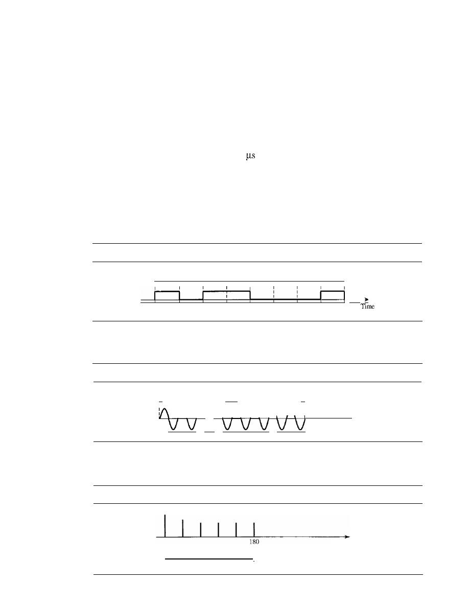
SECTION 3.10
PRACTICE SET
97
20. A periodic composite signal with a bandwidth of 2000 Hz is composed of two sine
waves. The first one has a frequency of 100 Hz with a maximum amplitude of 20 V;
the second one has a maximum amplitude of 5
V.
Draw the bandwidth.
21. Which signal has a wider bandwidth, a sine wave with a frequency of 100 Hz or a
sine wave with a frequency of 200 Hz?
22. What is the bit rate for each of the following signals?
a. A signal in which 1 bit lasts 0.001 s
b. A signal in which 1 bit lasts 2 ms
c. A signal in which 10 bits last 20
23. A device is sending out data at the rate of 1000 bps.
a. How long does it take to send out 10 bits?
b. How long does it take to send out a single character (8 bits)?
c. How long does it take to send a file of 100,000 characters?
24. What is the bit rate for the signal in Figure 3.34?
Figure 3.34
Exercise 24
16
ns
...
1
25. What is the frequency of the signal in Figure 3.35?
Figure 3.35
Exercise 25
Time
V
I,
4ms
.1
1
I
f\ f\ f\ f\
f\ f\ f\ : ...
26. What is the bandwidth of the composite signal shown in Figure 3.36.
Figure 3.36
Exercise 26
Frequency
5
5
5
5
5
I

CHAPTER
3
DATA AND SIGNALS
A periodic composite signal contains frequencies from 10 to 30 KHz, each with an
amplitude of 10
V. Draw the frequency spectrum.
A non-periodic composite signal contains frequencies from 10 to 30 KHz. The
peak amplitude is 10 V for the lowest and the highest signals and is 30 V for the
20-KHz signal. Assuming that the amplitudes change gradually from the minimum
to the maximum, draw the frequency spectrum.
A TV channel has a bandwidth of 6 MHz. If we send a digital signal using one
channel, what are the data rates if we use one harmonic, three harmonics, and
harmonics?
A signal travels from point A to point B. At point A, the signal power is 100 W. At
point B, the power is 90 W. What is the attenuation in decibels?
The attenuation of a signal is -10 dB. What is the final signal power if it was origi-
nally 5 W?
A signal has passed through three cascaded amplifiers, each with a 4 dB gain.
What is the total gain? How much is the signal amplified?
If
the bandwidth of the channel is 5 Kbps, how long does it take to send a frame of
100,000 bits out of this device?
The light of the sun takes approximately eight minutes to reach the earth. What is
the distance between the sun and the earth?
A signal has a wavelength of 1
in
air.
How far can the front of the wave travel
during 1000 periods?
A line has a signal-to-noise ratio of 1000 and a bandwidth of 4000 KHz. What is
the maximum data rate supported by this line?
We measure the performance of a telephone line (4 KHz of bandwidth). When the
signal is 10 V, the noise is 5 m
V. What is the maximum data rate supported by this
telephone line?
A file contains 2 million bytes. How long does it take to download this file using a
56-Kbps channel? 1-Mbps channel?
A computer monitor has a resolution of 1200 by 1000 pixels.
If
each pixel uses
1024 colors, how many bits are needed to send the complete contents of a screen?
A signal with 200 milliwatts power passes through 10 devices, each with an average
noise of 2 microwatts. What is the SNR? What is the SNR
dB
?
4
I.
If
the peak voltage value of a signal is 20 times the peak voltage value of the noise,
what is the SNR? What is the SNR
dB
?
What is the theoretical capacity of a channel in each of the following cases:
a. Bandwidth: 20 KHz
SNR
dB
=
40
b. Bandwidth: 200 KHz
SNR
dB
=
4
c. Bandwidth: 1 MHz
SNR
dB
=
20
We need to upgrade a channel to a higher bandwidth. Answer the following
questions:
a. How is the rate improved if we double the bandwidth?
b. How is the rate improved if we double the SNR?

SECTION 3.10
PRACTICE SET
99
We have a channel with 4 KHz bandwidth.
If
we want to send data at 100 Kbps,
what is the minimum SNR
dB
? What is SNR?
What is the transmission time of a packet sent by a station if the length of the
packet is 1 million bytes and the bandwidth of the channel is 200 Kbps?
46. What is the length of a bit in a channel with a propagation speed of 2 x 10
8
mls if
the channel bandwidth is
1 Mbps?
h. 10 Mbps?
100 Mbps?
7. How many bits can fit on a link with a 2 ms delay if the bandwidth of the link is
1 Mbps?
h. 10 Mbps?
100 Mbps?
What is the total delay (latency) for a frame of size 5 million bits that is being sent
on a link with 10 routers each having a queuing time of 2
and a processing time
of 1
The length of the link is 2000 Km. The speed of light inside the link is 2 x
10
8
mls.
The link has a bandwidth of 5 Mbps. Which component of the total delay
is dominant? Which one is negligible?

CHAPTER 4
Digital Transmission
A computer network is designed to send information from one point to another. This
information needs to be converted to either a digital signal or an analog signal for trans-
mission. In this chapter, we discuss the first choice, conversion to digital signals; in
Chapter 5, we discuss the second choice, conversion to analog signals.
We discussed the advantages and disadvantages of digital transmission over analog
transmission in Chapter 3. In this chapter, we show the schemes and techniques that
we use to transmit data digitally. First, we discuss digital-to-digital conversion tech-
niques, methods which convert digital data to digital signals. Second, we discuss analog-
to-digital conversion techniques, methods which change an analog signal to a digital
signaL Finally, we discuss transmission modes.
4.1
CONVERSION
In Chapter 3, we discussed data and signals. We said that data can be either digital or
analog. We also said that signals that represent data can also be digital or analog. In this
section, we see how we can represent digital data by using digital signals. The conver-
sion involves three techniques: line coding, block coding, and scrambling. Line coding
is always
block coding and scrambling mayor may not be needed.
Line Coding
Line coding is the process of converting digital data to digital signals. We assume that
data, in the form of text, numbers, graphical images, audio, or video, are stored in com-
puter memory as sequences of bits (see Chapter
1).
Line coding converts a sequence of
bits to a digital signal. At the sender, digital data are encoded into a digital signal; at the
receiver, the digital data are recreated by decoding the digital signal. Figure 4.1 shows
the process.
Characteristics
Before discussing different line coding schemes, we address their common characteristics.
101
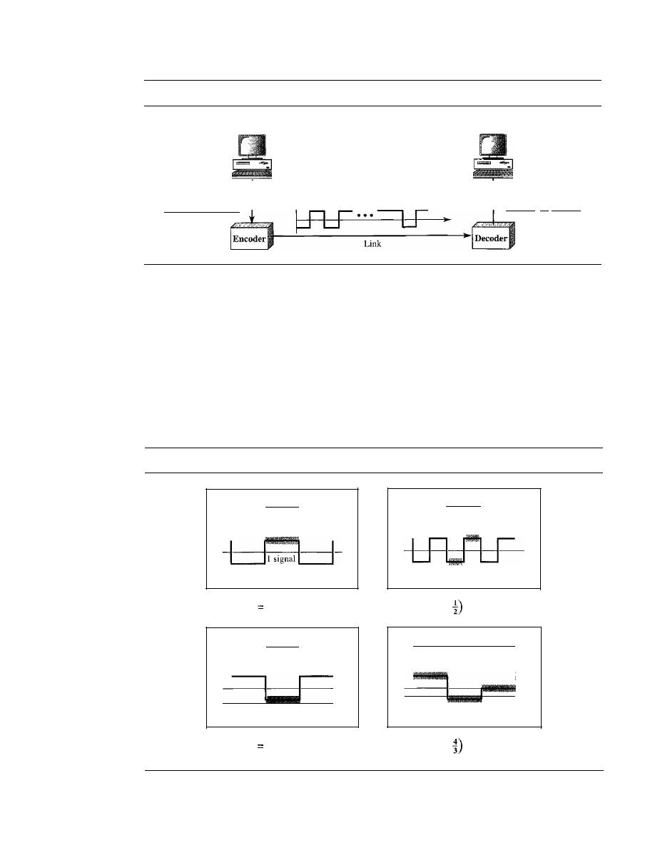
102
CHAPTER
4
DIGITAL TRANSMISSION
Figure 4.1
Line coding and decoding
Sender
Receiver
Digital data
1°101". 101
1
Digital signal
Digital data
1°101 •• ' 101 1
Signal Element Versus Data Element
Let us distinguish between a data element
and a signal element. In data communications, our goal is to send data elements. A
data element is the smallest entity that can represent a piece of information: this is the
bit. In digital data communications, a signal element carries data elements. A signal
element is the shortest unit (timewise) of a digital signal. In other words, data elements
are what we need to send; signal elements are what we can send. Data elements are
being carried; signal elements are the carriers.
We define a ratio
r
which is the number of data elements carried by each signal ele-
ment. Figure 4.2 shows several situations with different values of
r.
Figure 4.2
Signal element versus data element
I data element
I data element
o
o
element
2 signal
elements
a. One data element per one signal
element
(r
1)
b. One data element per two signal
elements
(r
=
2 data elements
4 data elements
1101
3 signal
elements
I signal
element
II
I
01
II
I
---'
c. Two data elements per one signal
element
(r
2)
d. Four data elements per three signal
elements
(r
=
In part a of the figure, one data element is carried by one signal element
(r
=
1). In
part b of the figure, we need two signal elements (two transitions) to carry each data

SECTION
4.1
DIGITAL-TO-DIGITAL CONVERSION
103
element
(r
=
! ).
We will see later that the extra signal element is needed to guarantee
2
synchronization. In part c of the figure, a signal element carries two data elements
(r
=
2).
Finally, in part d, a group of 4 bits is being carried by a group of three signal elements
(r
=
).
For every line coding scheme we discuss, we will give the value of
r.
3
.
An analogy may help here. Suppose each data element
IS
a person who needs to be
carried from one place to another. We can think of a signal element as a vehicle that can
carry people. When
r
=
1, it means each person is driving a vehicle. When
r
>
1, it
means more than one person is travelling in a vehicle (a carpool, for example). We can
also have the case where one person is driving a car and a trailer
(r
=
).
Data Rate Versus Signal Rate
The data rate defines the number of data elements
(bits) sent in Is. The unit is bits per second (bps). The signal rate is the number of sig-
nal elements sent in Is. The unit is the baud. There are several common terminologies
used in the literature. The data rate is sometimes called the bit rate; the signal rate is
sometimes called the pulse rate, the modulation rate, or the baud rate.
One goal in data communications is to increase the data rate while decreasing the
signal rate. Increasing the data rate increases the speed of transmission; decreasing the
signal rate decreases the bandwidth requirement. In our vehicle-people analogy, we
need to carry more people in fewer vehicles to prevent traffic jams. We have a limited
bandwidth
in our transportation system.
We now need to consider the relationship between data rate and signal rate (bit rate
and baud rate). This relationship, of course, depends on the value of
r.
It also depends
on the data pattern. If we have a data pattern of all 1s or all Os, the signal rate may be
different from a data pattern of alternating Os and Is. To derive a formula for the rela-
tionship, we need to define three cases: the worst, best, and average. The worst case is
when we need the maximum signal rate; the best case is when we need the minimum.
In data communications, we are usually interested in the average case. We can formu-
late the relationship between data rate and signal rate as
1
S
=c
xNx -
baud
r
where
N
is the data rate (bps); c is the case factor, which varies for each case; S is the
number of signal elements; and
r
is the previously defined factor.
Example 4.1
A signal is carrying data in which one data element is encoded as one signal element
(r
=
1). If
the bit rate is 100 kbps, what is the average value of the baud rate if c is between 0 and l?
Solution
We assume that the average value of c is
The baud rate is then
1 1 1
S
=
c
x N x -
= -
x 100,000 x -1
=
50,000
=
50 kbaud
r
2
Bandwidth
We discussed in Chapter 3 that a digital signal that carries infonnation is
nonperiodic. We also showed that the bandwidth of a nonperiodic signal is continuous
with an infinite range. However, most digital signals we encounter in real life have a

104
CHAPTER
4
DIGITAL TRANSMISSION
bandwidth with finite values. In other words, the bandwidth is theoretically infinite, but
many of the components have such a small amplitude that they can be ignored. The
effective bandwidth is finite. From now on, when we talk about the bandwidth of a dig-
ital signal, we need to remember that we are talking about this effective bandwidth.
Although the actual bandwidth ofa digital signal is infinite, the effective bandwidth is finite.
We can say that the baud rate, not the bit rate, determines the required bandwidth
for a digital signal.
If
we use the transpOltation analogy, the number of vehicles affects
the traffic, not the number of people being carried. More changes in the signal mean
injecting more frequencies into the signal. (Recall that frequency means change and
change means frequency.) The bandwidth reflects the range of frequencies we need.
There is a relationship between the baud rate (signal rate) and the bandwidth. Band-
width is a complex idea. When we talk about the bandwidth, we normally define a
range of frequencies. We need to know where this range is located as well as the values
of the lowest and the highest frequencies. In addition, the amplitude (if not the phase)
of each component is an impOltant issue. In other words, we need more information
about the bandwidth than just its value; we need a diagram of the bandwidth. We will
show the bandwidth for most schemes we discuss in the chapter. For the moment, we
can say that the bandwidth (range of frequencies) is proportional to the signal rate
(baud rate). The minimum bandwidth can be given as
1
B
min
N
-
r
We can solve for the maximum data rate if the bandwidth of the channel is given.
1
N
max
=
xBxr
Example 4.2
The maximum data rate of a channel (see Chapter 3) is
N
max
=
2
B
log2L (defined by the
Nyquist formula). Does this agree with the previous formula for
N
max
?
Solution
A signal with
L
levels actually can carry log2
L
bits per level.
If
each level corresponds to one sig-
nal element and we assume the average case (c
=
then we have
Baseline Wandering
In decoding a digital signal, the receiver calculates a running
average of the received signal power. This average is called the
baseline.
The incoming
signal power is evaluated against this baseline to determine the value of the data ele-
ment. A long string of Os or 1s can cause a drift in the baseline (baseline wandering)
and make it difficult for the receiver to decode correctly. A good line coding scheme
needs to prevent baseline wandering.
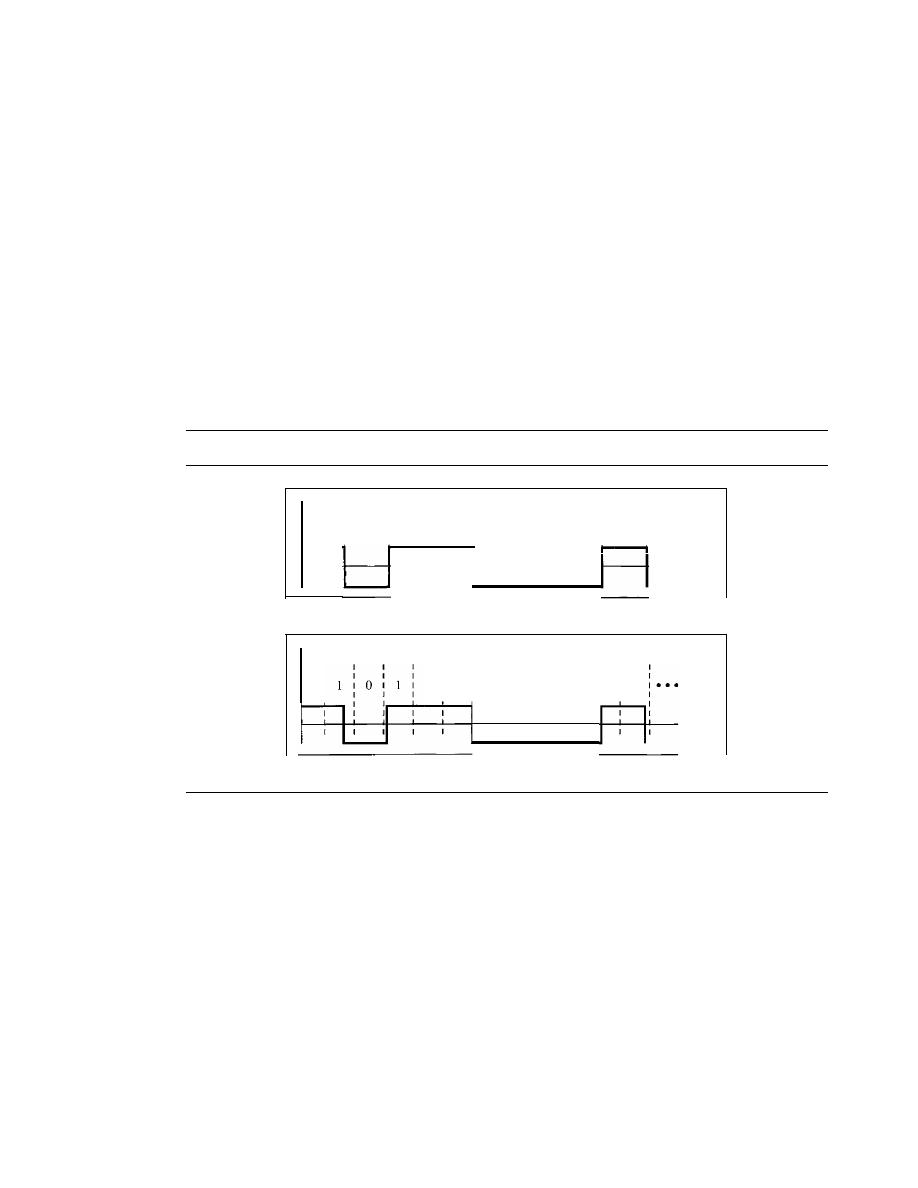
SECTION
4.1
DIGITAL-TO-DIGITAL CONVERSION
105
DC Components
When the voltage level in a digital signal is constant for a while,
the spectrum creates very low frequencies (results of Fourier analysis). These fre-
quencies around zero, called
DC
(direct-current)
components,
present problems for a
system that cannot pass low frequencies or a system that uses electrical coupling
(via a transformer). For example, a telephone line cannot pass frequencies below
200
Hz. Also a long-distance link may use one or more transformers to isolate
different parts of the line electrically. For these systems, we need a scheme with no
DC
component.
Self-synchronization
To correctly interpret the signals received from the sender,
the receiver's bit intervals must correspond exactly to the sender's bit intervals.
If
the
receiver clock is faster or slower, the bit intervals are not matched and the receiver might
misinterpret the signals. Figure 4.3 shows a situation in which the receiver has a shorter
bit duration. The sender sends
1011000 1,
while the receiver receives
110 111 0000 11.
Figure 4.3
Effect of lack ofsynchronization
a.Sent
J
o
I
I
I
o
J
I
o
:
0
:
J
I
I
I
Time
I
I
1
I
I
b. Received
I
I
1
I
1
0
0
0
0
I
I
I
1
I
1
I
Time
A
self-synchronizing digital signal includes timing information in the data being
transmitted. This can be achieved if there are transitions in the signal that alert the
receiver to the beginning, middle, or end of the pulse.
If
the receiver's clock is out of
synchronization, these points can reset the clock.
Example 4.3
In a digital transmission, the receiver clock is 0.1 percent faster than the sender clock. How many
extra bits per second does the receiver receive if the data rate is 1 kbps? How many if the data
rate is 1 Mbps?
Solution
At
1
kbps, the receiver receives
1001
bps instead of
1000
bps.
1000 bits sent
1001
bits
received
1
extra bps
106
CHAPTER
4
DIGITAL TRANSMISSION
At 1 Mbps, the receiver receives 1,001,000 bps instead
of
1,000,000 bps.
1,000,000
sent
1,001,000 bits
1000 extra bps
Built-in Error Detection
It is desirable to have a built-in error-detecting capability
in the generated code to detect some of or all the errors that occurred during transmis-
sion. Some encoding schemes that we will discuss have this capability to some extent.
Immunity to Noise and Interference
Another desirable code characteristic is a code
I
that is immune to noise and other interferences. Some encoding schemes that we will
discuss have this capability.
Complexity
A complex scheme is more costly to implement than a simple one. For
example, a scheme that uses four signal levels is more difficult to interpret than one that
uses only two levels.
Line Coding Schemes
We can roughly divide line coding schemes into five broad categories, as shown in
Figure 4.4.
Figure 4.4
Line coding schemes
Multitransition
- - MLT-3
Multilevel
- - 2B/IQ, 8B/6T, and 4U-PAM5
Line coding
Unipolar
Polar
Bipolar
- - N R Z
NRZ,
and biphase (Manchester.
and differential Manchester)
- - AMI and pseudoternary
There are several schemes in each category. We need to be familiar with all
schemes discussed in this section to understand the rest of the book. This section can be
used as a reference for schemes encountered later.
Unipolar Scheme
In a unipolar scheme, all the signal levels are on one side of the time axis, either above
or below.
NRZ (Non-Return-to-Zero)
Traditionally, a unipolar scheme was designed as a
non-return-to-zero (NRZ) scheme in which the positive voltage defines bit I and the
zero voltage defines bit O.
It
is called NRZ because the signal does not return to zero at
the middle of the bit. Figure 4.5 show a unipolar NRZ scheme.
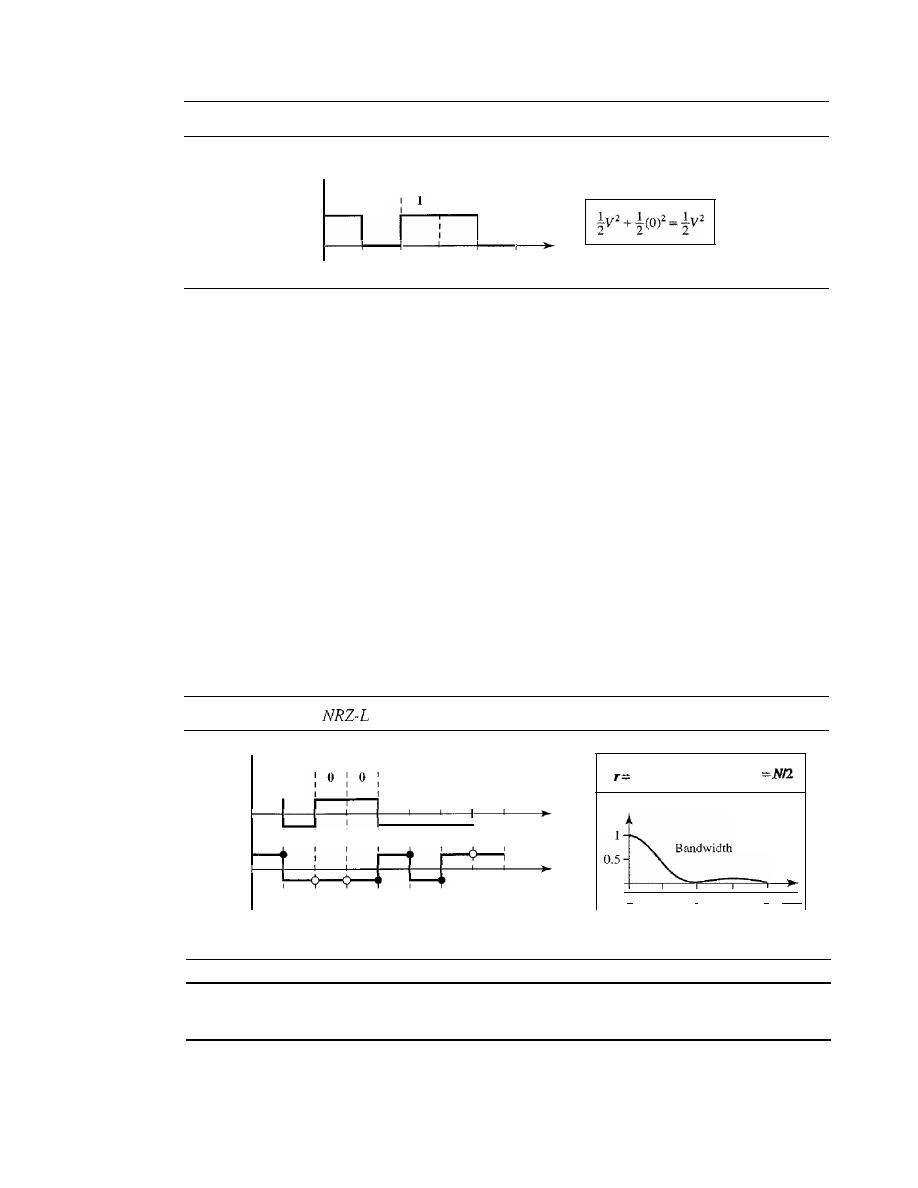
SECTION 4.1
DIGITAL-TO-DIGITAL CONVERSION
107
Figure 4.5
Unipolar NRZ scheme
Amplitude
v
1
f
0
f
:
1
I
0
I
o
I
Time
Nonnalized power
Compared with its polar counterpart (see the next section), this scheme is very
costly. As we will see shortly, the normalized power (power needed to send 1 bit per
unit line resistance) is double that for polar NRZ. For this reason, this scheme is nor-
mally not used in data communications today.
Polar Schemes
In polar schemes, the voltages are on the both sides of the time axis. For example, the
voltage level for 0 can be positive and the voltage level for I can be negative.
Non-Return-to-Zero (NRZ)
In polar NRZ encoding, we use two levels of voltage
amplitude. We can have two versions of polar NRZ: NRZ-Land NRZ-I, as shown in
Figure 4.6. The figure also shows the value of
r,
the average baud rate, and the band-
width. In the first variation, NRZ-L (NRZ-Level), the level of the voltage determines
the value of the bit. In the second variation, NRZ-I (NRZ-Invert), the change or lack of
change in the level of the voltage determines the value of the bit.
If
there is no change,
the bit is 0; if there is a change, the bit is 1.
Figure 4.6
Polar
and NRZ-I schemes
1
Save
p
o
o
I
2
fIN
Time
Time
1 : 1
0
I
I
0 1 1
I
I
NRZ-I
NRZ-L
o
No inversion: Next bit is 0
• Inversion: Next bit is 1
In NRZ-L the level of the voltage determines the value of the bit. In NRZ-I
the inversion or the lack of inversion determines the value of the bit.
Let us compare these two schemes based on the criteria we previously defined.
Although baseline wandering is a problem for both variations, it is twice as severe in
NRZ-
L. If
there is a long sequence of Os or I s in NRZ-L, the average signal power

108
CHAPTER
4
DIGITAL TRANSMISSION
becomes skewed. The receiver might have difficulty discerning the bit value. In NRZ-I
this problem occurs only for a long sequence of as.
If
somehow we can eliminate the
long sequence of as, we can avoid baseline wandering. We will see shortly how this can
be done.
The synchronization problem (sender and receiver clocks are not synchronized)
also exists in both schemes. Again, this problem is more serious in NRZ-L than in
NRZ- I. While a long sequence of as can cause a problem in both schemes, a long
sequence of 1s affects only NRZ-L.
Another problem with NRZ-L occurs when there is a sudden change of polarity in
the system. For example, if twisted-pair cable is the medium, a change in the polarity of
the wire results in all as interpreted as I s and all I s interpreted as as. NRZ-I does not
have this problem. Both schemes have an average signal rate of
NI2
Bd.
NRZ-L and NRZ-J both have an average signal rate of
NI2
Bd.
Let us discuss the bandwidth. Figure 4.6 also shows the normalized bandwidth for
both variations. The vertical axis shows the power density (the power for each I Hz of
bandwidth); the horizontal axis shows the frequency. The bandwidth reveals a very
serious problem for this type of encoding. The value of the power density is velY high
around frequencies close to zero. This means that there are
DC
components that carry a
high level of energy. As a matter of fact, most of the energy is concentrated in frequen-
cies between a and
NIl.
This means that although the average of the signal rate is
N12,
the energy is not distributed evenly between the two halves.
NRZ-L and NRZ-J both have a
DC
component problem.
Example 4.4
A
system is using NRZ-I to transfer 10-Mbps data. What are the average signal rate and mini-
mum bandwidth?
Solution
The average signal rate is
S
=
NI2
=
500 kbaud. The minimum bandwidth
for
this average baud
rate is
=
S
=
500
kHz.
Return to Zero (RZ)
The main problem with NRZ encoding occurs when the sender
and receiver clocks are not synchronized. The receiver does not know when one bit has
ended and the next bit is starting. One solution is the return-to-zero (RZ) scheme,
which uses three values: positive, negative, and zero. In RZ, the signal changes not
between bits but during the bit. In Figure 4.7 we see that the signal goes to
0
in the mid-
dle of each bit.
It
remains there until the beginning of the next bit. The main disadvan-
tage of RZ encoding is that it requires two signal changes to encode a bit and therefore
occupies greater bandwidth. The same problem we mentioned, a sudden change of
polarity resulting in all as interpreted as 1s and all 1s interpreted as as, still exist here,
but there is no
DC
component problem. Another problem is the complexity: RZ uses
three levels of voltage, which is more complex to create and discern. As a result of all
these deficiencies, the scheme is not used today. Instead, it has been replaced by the
better-performing Manchester and differential Manchester schemes (discussed next).
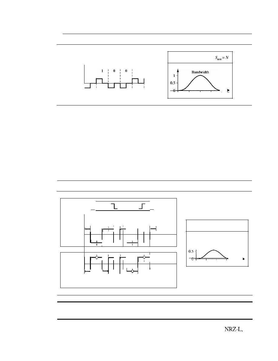
SECTION
4.1
DIGITAL-TO-DIGITAL CONVERSION
109
Figure 4.7
Polar RZ scheme
Amplitude
o
l
l
l
1
l
1
l
Time
p
o
I
o
1
2 fiN
Biphase: Manchester and Differential Manchester
The idea of RZ (transition at
the middle of the bit) and the idea of NRZ-L are combined into the Manchester scheme.
In Manchester encoding, the duration of the bit is divided into two halves. The voltage
remains at one level during the first half and moves to the other level in the second half.
The transition at the middle of the bit provides synchronization. Differential Manchester,
on the other hand, combines the ideas of RZ and NRZ-I. There is always a transition at
the middle of the bit, but the bit values are determined at the beginning of the bit.
If
the
next bit is
0,
there is a transition; if the next bit is
1,
there is none. Figure
4.8
shows
both Manchester and differential Manchester encoding.
Figure 4.8
Polar biphase: Manchester and differential Manchester schemes
(
Ois
lis
)
0
I
1
I
0
I
0
I
1
I
1
I
I
I
I
I
I
I
I
I
I
I
I
I
I
I
_,
I
1
I
I
I
I
Manchester
I
I
I
I
Time
I
- I
I -
I
I
I
I
I
l
I
I
I
I
I
I
I
Differential
I
I
I
Manchester
I
I
I
I
Time
1
I
I
1
-
I
1
I
I
I
I
I
o
No inversion: Next bit is 1
• Inversion: Next bit is 0
p
11
Bandwidth
o
1
2
fiN
In Manchester and differential Manchester encoding, the transition
at the middle of the bit is used for synchronization.
The Manchester scheme overcomes several problems associated with
and
differential Manchester overcomes several problems associated with NRZ-
I.
First, there
is no baseline wandering. There is no
DC
component because each bit has a positive and
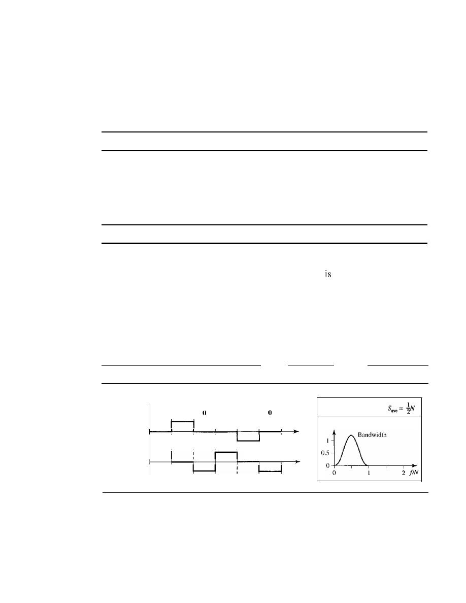
110
CHAPTER
4
DIGITAL TRANSMISSION
negative voltage contribution. The only drawback is the signal rate. The signal rate for
Manchester and differential Manchester is double that for NRZ. The reason is that there is
always one transition at the middle of the bit and maybe one transition at the end of each
bit. Figure 4.8 shows both Manchester and differential Manchester encoding schemes.
Note that Manchester and differential Manchester schemes are also called biphase
schemes.
The minimum bandwidth of Manchester and differential Manchester is 2 times that of NRZ.
Bipolar Schemes
In bipolar encoding (sometimes called
multilevel binary),
there are three voltage lev-
els: positive, negative, and zero. The voltage level for one data element is at zero, while
the voltage level for the other element alternates between positive and negative.
In bipolar encoding, we use three levels: positive, zero, and negative.
AMI and Pseudoternary
Figure 4.9 shows two variations of bipolar encoding: AMI
and pseudoternary. A common bipolar encoding scheme
called bipolar alternate
mark inversion (AMI). In the term
alternate mark inversion,
the word
mark
comes
from telegraphy and means 1. So AMI means alternate I inversion. A neutral zero volt-
age represents binary O. Binary Is are represented by alternating positive and negative
voltages. A variation of AMI encoding is called pseudoternary in which the
1
bit is
encoded as a zero voltage and the 0 bit is encoded as alternating positive and negative
voltages.
Figure 4.9
Bipolar schemes: AMI and pseudoternary
Amplitude
o
I
I
I
I
o
I
I
I
I
:
I
I
r=
1
p
Time
Time
AMI
Pseudoternary
The bipolar scheme was developed as an alternative to NRZ. The bipolar scheme
has the same signal rate as NRZ, but there is no
DC
component. The NRZ scheme has
most of its energy concentrated near zero frequency, which makes it unsuitable for
transmission over channels with poor performance around this frequency. The concen-
tration of the energy in bipolar encoding is around frequency
N12.
Figure 4.9 shows the
typical energy concentration for a bipolar scheme.

SECTION
4.1
DIGITAL-TO-DIGITAL CONVERSION
111
One may ask why we do not have
DC
component in bipolar encoding. We can
answer this question by using the Fourier transform, but we can also think about it intu-
itively.
If
we have a long sequence of 1s, the voltage level alternates between positive
and negative; it is not constant. Therefore, there is no
DC
component. For a long
sequence of Os, the voltage remains constant, but its amplitude is zero, which is the
same as having no
DC
component. In other words, a sequence that creates a constant
zero voltage does not have a
DC
component.
AMI is commonly used for long-distance communication, but it has a synchroniza-
tion problem when a long sequence of Os is present in the data. Later in the chapter, we
will see how a scrambling technique can solve this problem.
Multilevel Schemes
The desire to increase the data speed or decrease the required bandwidth has resulted in
the creation of many schemes. The goal is to increase the number of bits per baud by
encoding a pattern of m data elements into a pattern of n signal elements. We only have
two types of data elements (Os and Is), which means that a group of
m
data elements
can produce a combination of
2
m
data patterns. We can have different types of signal
elements by allowing different signal levels. If we have L different levels, then we can
produce L
n
combinations of signal patterns. If 2
m
=
L
n,
then each data pattern is
encoded into one signal pattern. If 2
m
<
L
n
,
data patterns occupy only a subset of signal
patterns. The subset can be carefully designed to prevent baseline wandering, to pro-
vide synchronization, and to detect errors that occurred during data transmission. Data
encoding is not possible if 2
m
>
L
n
because some of the data patterns cannot be
encoded.
The code designers have classified these types of coding as mBnL, where m is the
length of the binary pattern,
B
means binary data,
n
is the length of the signal pattern,
and
L
is the number of levels in the signaling. A letter is often used in place of
L:
B
(binary) for L
=
2, T (ternary) for L
=
3, and Q (quaternary) for L
=
4. Note that the first
two letters define the data pattern, and the second two define the signal pattern.
In
mBnL schemes, a pattern of m data elements is encoded as a pattern of n signal
elements in which
Ln.
2BIQ
The first mBnL scheme we discuss,
two binary, one quaternary (2BIQ),
uses
data patterns of size 2 and encodes the 2-bit patterns as one signal element belonging
to a four-level signal. In this type of encoding
m
=
2,
n
=
1, and
L
=
4 (quatemary). Fig-
ure 4.10 shows an example of a 2B 1Q signal.
The average signal rate of 2BlQ is S
=
N/4.
This means that using 2BIQ, we can
send data 2 times faster than by using NRZ-L. However, 2B lQ uses four different sig-
nal levels, which means the receiver has to discern four different thresholds. The
reduced bandwidth comes with a price. There are no redundant signal patterns in this
scheme because 2
2
=
4
1
.
As we will see in Chapter 9, 2BIQ is used in DSL (Digital Subscriber Line) tech-
nology to provide a high-speed connection to the Internet by using subscriber telephone
lines.
112
CHAPTER
4
DIGITAL TRANSMISSION
Figure 4.10
Multilevel: 2B1Q scheme
Previous level:
Previous level:
positive
negative
Next
Next
Next
bits
level
level
00
+1
-I
01
+3
-3
10
-I
+1
II
-3
+3
Transition table
2 fiN
Save
=N14
o
1/2
p
1 \
Bandwidth
0.5
o
me
00
I
II
0]
I
HI
I
0]
I
I
I
I
I
I
I
I
I
I
I
I
Ti
I
I
I
I
I
I
I
I
I
I
,
+3
-3
+1
Assuming positive original level
8B6T
A very interesting scheme is
eight binary,
six
ternary
(8B6T). This code
used
with 100BASE-4T cable, as we will see in Chapter 13. The idea is to encode a pattern of
8 bits as a pattern of 6 signal elements, where the signal has three levels (ternary). In this
type of scheme, we can have 2
8
=
256 different data patterns and 3
6
=
478 different signal
patterns. The mapping table is shown in Appendix D. There are 478 - 256
=
222 redundant
signal elements that provide synchronization and error detection. Part of the redundancy is
also used to provide
DC
balance. Each signal pattern has a weight of 0 or +1
DC
values. This
means that there is no pattern with the weight
-1. To make the whole stream Dc-balanced,
the sender keeps track of the weight. If two groups of weight 1 are encountered one after
another, the first one is sent as is, while the next one is totally inverted to give a weight of -1.
Figure 4.11 shows an example of three data patterns encoded as three signal pat-
terns. The three possible signal levels are represented as -,0, and +. The first 8-bit
tern 00010001 is encoded as the signal pattern -0-0++ with weight 0; the second 8-bit
pattern 010 10011 is encoded as - + - + + 0 with weight + 1. The third bit pattern should
be encoded as + - - + 0
+
with weight
+
1. To create DC balance, the sender inverts the
actual signal. The receiver can easily recognize that this is an inverted pattern because
the weight is -1. The pattern is inverted before decoding.
Figure 4.11
Multilevel: 8B6T scheme
Time
01()10011
OOOIO()O(
O!OIOO()()
I
I
pattern :
o
+v
-v
-0-0++
-+-++0
+--+0+
SECTION
4.1
DIGITAL-TO-DIGITAL CONVERSION
113
The average signal rate of the scheme is theoretically
Save
=
X
N
X
in practice
the minimum bandwidth is very close to
6N18.
2
8
4D-PAMS
The last signaling scheme we discuss in this category is called four-
dimensional five-level pulse amplitude modulation (4D-PAM5). The 4D means that data
is sent over four wires at the same time.
It
uses five voltage levels, such as -2,
0, 1, and 2.
However, one level, level 0, is used only for forward error detection (discussed in Chap-
ter 10).
If
we assume that the code is just one-dimensional, the four levels create something
similar to 8B4Q.
In
other words, an 8-bit word is translated to a signal element of four differ-
ent levels. The worst signal rate for this imaginary one-dimensional version is
N
X
4/8,
or
N12.
The technique is designed to send data over four channels (four wires). This means
the signal rate can be reduced to
N18,
a significant achievement. All 8 bits can be fed into a
wire simultaneously and sent by using one signal element. The point here is that the four
signal elements comprising one signal group are sent simultaneously in a four-dimensional
setting. Figure 4.12 shows the imaginary one-dimensional and the actual four-dimensional
implementation. Gigabit LANs (see Chapter 13) use this technique to send 1-Gbps data
over four copper cables that can handle 125 Mbaud. This scheme has a lot of redundancy
in the signal pattern because 2
8
data patterns are matched to 4
4
=
256 signal patterns. The
extra signal patterns can be used for other purposes such as error detection.
Figure 4.12
Multilevel: 4D-PAM5 scheme
00011110
1 Gbps
250 Mbps
Wire 1 (125 MBd)
250 Mbps
Wire 2 (125 MBd)
+2
+1
250 Mbps
Wire 3 (125 MBd)
-1
250 Mbps
Wire 4 (125 MBd)
Multiline Transmission: MLT-3
NRZ-I and differential Manchester are classified as differential encoding but use two transi-
tion rules to encode binary data (no inversion, inversion).
If
we have a signal with more than
two levels, we can design a differential encoding scheme with more than two transition
rules. MLT-3 is one of them. The multiline transmission, three level (MLT-3) scheme
uses three levels
(+
v,
0, and -
V)
and three transition rules to move between the levels.
1.
If the next bit is 0, there is no transition.
2.
If
the next bit is 1 and the current level is not 0, the next level is 0.
3.
If
the next bit is 1 and the cutTent level is 0, the next level is the opposite of the last
nonzero level.
114
CHAPTER
4
DIGITAL TRANSMISSION
The behavior of MLT-3 can best be described by the state diagram shown in Figure 4.13.
The three voltage levels
(-V,
0, and
+V)
are shown by three states (ovals). The transition
from one state (level) to another is shown by the connecting lines. Figure 4.13 also
shows two examples of an MLT-3 signal.
Figure
4.13
Multitransition: MLT-3 scheme
Last
non-zero
non-zero
Next bit: 0
level:
+
V
level: -
V
Next bit: 0
Next bit: 0
Next bit: 1
c. Transition states
: Time
1
I
0 1 1 1 0 1 1 1 1 0 1 1 1 1
1
I
I
I
I
1
+V
I
I
I
I
I
I
OV
- - - t -
1
OV
+v
-v
-v
b. Worse case
a. Typical case
One might wonder why we need to use MLT-3, a scheme that maps one bit to one
signal element. The signal rate is the same as that for
NRZ-I, but with greater complexity
(three levels and complex transition rules). It turns out that the shape of the signal in this
scheme helps to reduce the required bandwidth. Let us look at the worst-case scenario, a
sequence of
I
s. In this case, the signal element pattern
+
VO - VO
is repeated every
4
bits.
A
nonperiodic signal has changed to a periodic signal with the period equal to
4
times the
bit duration. This worst-case situation can be simulated as an analog signal with a fre-
quency one-fourth of the bit rate. In other words, the signal rate for MLT-3 is one-fourth
the bit rate. This makes MLT-3 a suitable choice when we need to send 100 Mbps on a
copper wire that cannot support more than 32 MHz (frequencies above this level create
electromagnetic emissions). MLT-3 and LANs are discussed in Chapter 13.
Summary of Line Coding Schemes
We summarize in Table 4.1 the characteristics of the different schemes discussed.
Table 4.1
Summary of line coding schemes
Bandwidth
Category
Scheme
(average)
Characteristics
Unipolar
NRZ
B=N/2
Costly, no self-synchronization iflong Os or Is,
DC
NRZ-L
B=N/2
No self-synchronization if long Os or 1s,
DC
Unipolar
NRZ-I
B=N/2
No self-synchronization for long
aS,
DC
Biphase
B=N
Self-synchronization, no
DC,
high bandwidth
SECTION 4.1
DIGITAL-TO-DIGITAL CONVERSION
115
Table 4.1
Summary of line coding schemes (continued)
Bandwidth
Category
Scheme
(average)
Characteristics
Bipolar
AMI
B=NI2
No self-synchronization for long
OS, DC
2BIQ
B=N/4
No self-synchronization for long same double bits
Multilevel
8B6T
B
=
3N/4
Self-synchronization, no
DC
4D-PAM5
B=N/8
Self-synchronization, no
DC
Multiline
MLT-3
B=N/3
No self-synchronization for long Os
Block Coding
We need redundancy to ensure synchronization and to provide some kind of inherent
error detecting. Block coding can give us this redundancy and improve the perfor-
mance of line coding. In general, block coding changes a block of
m
bits into a block
of
n
bits, where
n
is larger than
m.
Block coding is referred to as an
mB/nB
encoding
technique.
Block coding is normally referred to as
mBlnB coding;
it replaces each
group with an
group.
The slash in block encoding (for example, 4B/5B) distinguishes block encoding
from multilevel encoding (for example, 8B6T), which is written without a slash. Block
coding normally involves three steps: division, substitution, and combination. In the
division step, a sequence of bits is divided into groups of
m
bits. For example, in 4B/5B
encoding, the original bit sequence is divided into 4-bit groups. The heart of block cod-
ing is the substitution step. In this step, we substitute an m-bit group for an n-bit group.
For example, in 4B/5B encoding we substitute a 4-bit code for a 5-bit group. Finally,
the n-bit groups are combined together to form a stream. The new stream has more bits
than the original bits. Figure 4.14 shows the procedure.
Figure 4.14
Block coding concept
Division of a stream into m-bit groups
m bits
m bits
m bits
[110"'111000'''11 ••• 1010'''11
substitu
1010"'10111000'''00 1
1... 1°
11 ''.1111
n bits
n bits
n
bits
Combining n-bit groups into a stream
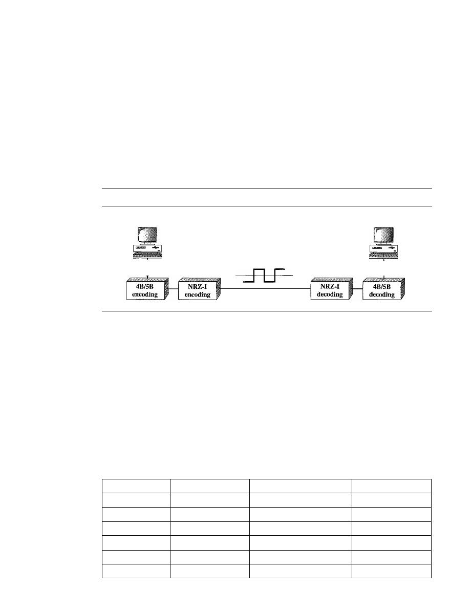
116
CHAPTER
4
DIGITAL TRANSMISSION
4B/5B
The four binary/five binary (4B/5B) coding scheme was designed to be used in com-
bination with NRZ-I. Recall that NRZ-I has a good signal rate, one-half that of the
biphase, but it has a synchronization problem. A long sequence of as can make the
receiver clock lose synchronization. One solution is to change the bit stream, prior to
encoding with NRZ-I, so that it does not have a long stream of as. The 4B/5B scheme
achieves this goal. The block-coded stream does not have more that three consecutive
as, as we will see later. At the receiver, the NRZ- I encoded digital signal is first
decoded into a stream of bits and then decoded to remove the redundancy. Figure 4.15
shows the idea.
Figure 4.15
Using block coding 4B/5B with NRZ-I line coding scheme
Sender
Receiver
Digital signal
Link
In 4B/5B, the 5-bit output that replaces the 4-bit input has no more than one leading
zero (left bit) and no more than two trailing zeros (right bits). So when different groups
are combined to make a new sequence, there are never more than three consecutive
as.
(Note that NRZ-I has no problem with sequences of Is.) Table 4.2 shows the corre-
sponding pairs used in 4B/5B encoding. Note that the first two columns pair a 4-bit
group with a 5-bit group. A group of 4 bits can have only 16 different combinations
while a group of 5 bits can have 32 different combinations. This means that there are 16
groups that are not used for 4B/5B encoding. Some of these unused groups are used for
control purposes; the others are not used at all. The latter provide a kind of error detec-
tion.
If
a 5-bit group arrives that belongs to the unused portion of the table, the receiver
knows that there is an error in the transmission.
Table 4.2
4B/5B mapping codes
Data Sequence
Encoded Sequence
Control Sequence
Encoded Sequence
0000
11110
Q (Quiet)
00000
0001
01001
I (Idle)
11111
0010
10100
H (Halt)
00100
0011
10101
J
(Start delimiter)
11000
0100
01010
K (Start delimiter)
10001
0101
01011
T (End delimiter)
01101
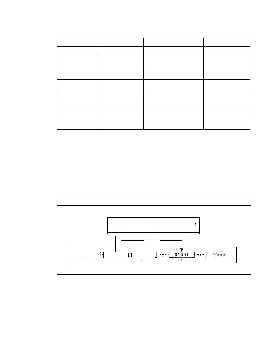
SECTION
4.1
DIGITAL-TO-DIGITAL CONVERSION
117
Table 4.2
4B/5B mapping codes (continued)
Data Sequence
Encoded Sequence
Control Sequence
Encoded Sequence
0110
01110
S (Set)
11001
0111
01111
R (Reset)
00111
1000
10010
1001
10011
1010
10110
1011
10111
1100
11 010
1101
11011
1110
11100
1111
11101
Figure
4.16
shows an example of substitution in
4B/5B
coding.
4B/5B
encoding
solves the problem of synchronization and overcomes one of the deficiencies of
NRZ-1.
However, we need to remember that it increases the signal rate of NRZ-
1.
The redun-
dant bits add 20 percent more baud. Still, the result is less than the biphase scheme
which has a signal rate of
2
times that of
NRZ-1.
However,
4B/5B
block encoding does
not solve the
DC
component problem of
NRZ-1.
If
a
DC
component is unacceptable, we
need to use biphase
or
bipolar encoding.
Figure 4.16
Substitution in 48/5B block coding
4-bit blocks
I
1 1 1 1
I •••
I
000 I
I I
0000
I
1 1 1 1 1
1 1 1 1 0
I
1 1 1 0 1
I
r
5-bit blocks
Example 4.5
We need to send data at a 1-Mbps rate. What is the minimum required bandwidth, using a combi-
nation of
4B/5B
and NRZ-I or Manchester coding?
Solution
First
4B/5B
block coding increases the bit rate to 1.25 Mbps. The minimum bandwidth using
NRZ-I is NI2 or 625 kHz. The Manchester scheme needs a minimum bandwidth of 1 MHz. The
first choice needs a lower bandwidth, but has a
DC
component problem; the second choice needs
a higher bandwidth, but does not have a
DC
component problem.
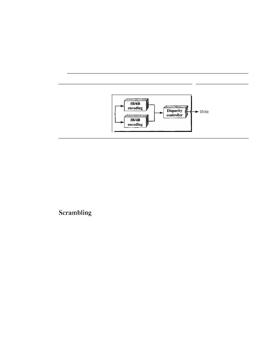
118
CHAPTER
4
DIGITAL TRANSMISSION
8RIlOR
The eight binary/ten binary (SBIlOB) encoding is similar to 4B/5B encoding except
that a group of 8 bits of data is now substituted by a lO-bit code.
It
provides greater
error detection capability than 4B/5B. The 8BIlOB block coding is actually a combina-
tion of 5B/6B and 3B/4B encoding, as shown in Figure 4.17.
Figure 4.17
8B/lOB block encoding
8B/IOB encoder
8-bit block
block
The most five significant bits of a 10-bit block is fed into the 5B/6B encoder; the
least 3 significant bits is fed into a 3B/4B encoder. The split is done to simplify the
mapping table. To prevent a long run of consecutive Os or Is, the code uses a disparity
controller which keeps track of excess Os over Is (or Is over Os).
If
the bits in the cur-
rent block create a disparity that contributes to the previous disparity (either direction),
then each bit in the code is complemented (a 0 is changed to a 1 and a 1 is changed to a 0).
The coding has 2
10
-
2
8
=
768 redundant groups that can be used for disparity checking
and error detection. In general, the technique is superior to 4B/5B because of better
built-in error-checking capability and better synchronization.
Biphase schemes that are suitable for dedicated links between stations in a LAN are not
suitable for long-distance communication because of their wide bandwidth requirement.
The combination of block coding and NRZ line coding is not suitable for long-distance
encoding either, because of the
DC
component. Bipolar AMI encoding, on the other
hand, has a narrow bandwidth and does not create a
DC
component. However, a long
sequence of Os upsets the synchronization.
If
we can find a way to avoid a long sequence
of Os in the original stream, we can use bipolar AMI for long distances. We are looking
for a technique that does not increase the number of bits and does provide synchroniza-
tion. We are looking for a solution that substitutes long zero-level pulses with a combi-
nation of other levels to provide synchronization. One solution is called scrambling. We
modify part of the AMI rule to include scrambling, as shown in Figure 4.18. Note that
scrambling, as opposed to block coding, is done at the same time as encoding. The
system needs to insert the required pulses based on the defined scrambling rules. Two
common scrambling techniques are B8ZS and HDB3.
R8ZS
Bipolar with S-zero substitution (BSZS) is commonly used in North America. In
this technique, eight consecutive zero-level voltages are replaced by the sequence
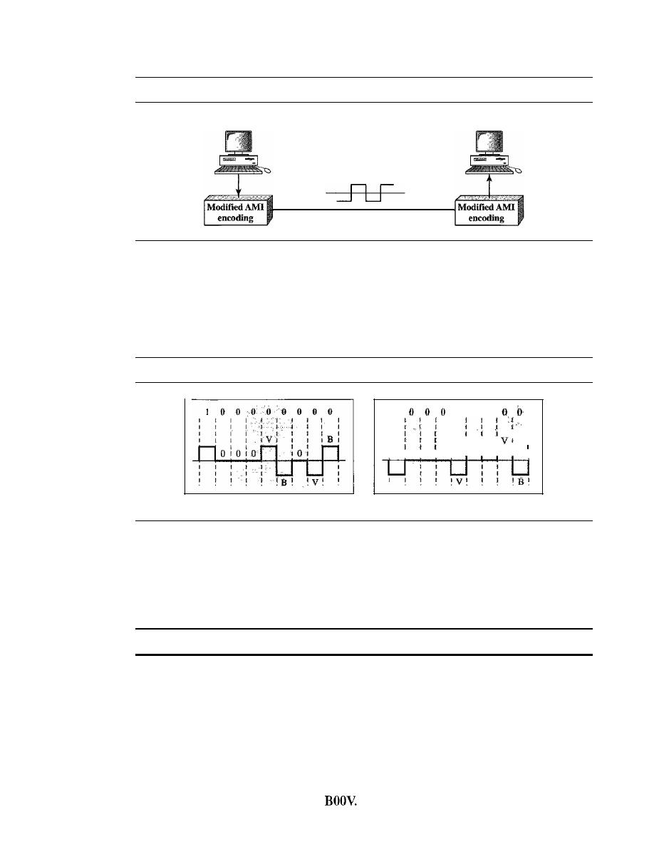
SECTION
4.1
DIGITAL-TO-DIGITAL CONVERSION
119
Figure 4.18
AMI used with scrambling
Sender
Receiver
Violated digital signal
OOOVBOVB.
The V in the sequence denotes violation; this is a nonzero voltage that
breaks an AMI rule of encoding (opposite polarity from the previous). The B in the
sequence denotes bipolm; which means a nonzero level voltage in accordance with the
AMI rule. There are two cases, as shown in Figure 4.19.
Figure 4.19
Two cases ofB8ZS scrambling technique
I
0 0 0
:
1
1
I
B
I
I
':1
I
10 10 101
0
I
a. Previous level is positive.
b. Previous level is negative.
Note that the scrambling in this case does not change the bit rate. Also, the tech-
nique balances the positive and negative voltage levels (two positives and two nega-
tives), which means that the
DC
balance is maintained. Note that the substitution may
change the polarity of a 1 because, after the substitution, AMI needs to follow its rules.
B8ZS substitutes eight consecutive zeros with OOOVBOVB.
One more point is worth mentioning. The letter V (violation) or B (bipolar) here is
relative. The V means the same polarity as the polarity of the previous nonzero pulse; B
means the polarity opposite to the polarity of the previous nonzero pulse.
HDB3
High-density bipolar 3-zero (HDB3) is commonly used outside of North America. In this
technique, which is more conservative than B8ZS, four consecutive zero-level voltages are
replaced with a sequence of OOOV or
The reason for two different substitutions is to
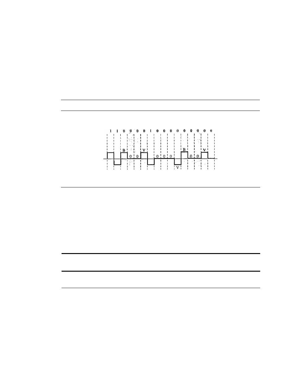
120
CHAPTER
4
DIGITAL TRANSMISSION
maintain the even number of nonzero pulses after each substitution. The two rules can be
stated as follows:
1. If the number of nonzero pulses after the last substitution is odd, the substitution
pattern will be OOOV, which makes the total number of nonzero pulses even.
2.
If
the number of nonzero pulses after the last substitution is even, the substitution
pattern will be BOOV, which makes the total number of nonzero pulses even.
Figure 4.20 shows an example.
Figure 4.20
Different situations in HDB3 scrambling technique
First
substitution
Second
Third
substitution
substitution
t
Even
t t
Even Odd
Even
Even
There are several points we need to mention here. First, before the first substitu-
tion, the number of nonzero pulses is even, so the first substitution is BODY. After this
substitution, the polarity of the 1 bit is changed because the AMI scheme, after each
substitution, must follow its own rule. After this bit, we need another substitution,
which is OOOV because we have only one nonzero pulse (odd) after the last substitution.
The third substitution is BOOV because there are no nonzero pulses after the second
substitution (even).
HDB3 substitutes four consecutive zeros with OOOV or BOOV depending
on the number of nonzero pulses after the last substitution.
4.2
ANALOG-TO-DIGITAL CONVERSION
The techniques described in Section 4.1 convert digital data to digital signals. Some-
times, however, we have an analog signal such as one created by a microphone or cam-
era. We have seen in Chapter 3 that a digital signal is superior to an analog signal. The
tendency today is to change an analog signal to digital data. In this section we describe
two techniques, pulse code modulation and delta modulation. After the digital data are
created (digitization), we can use one of the techniques described in Section 4.1 to con-
vert the digital data to a digital signal.
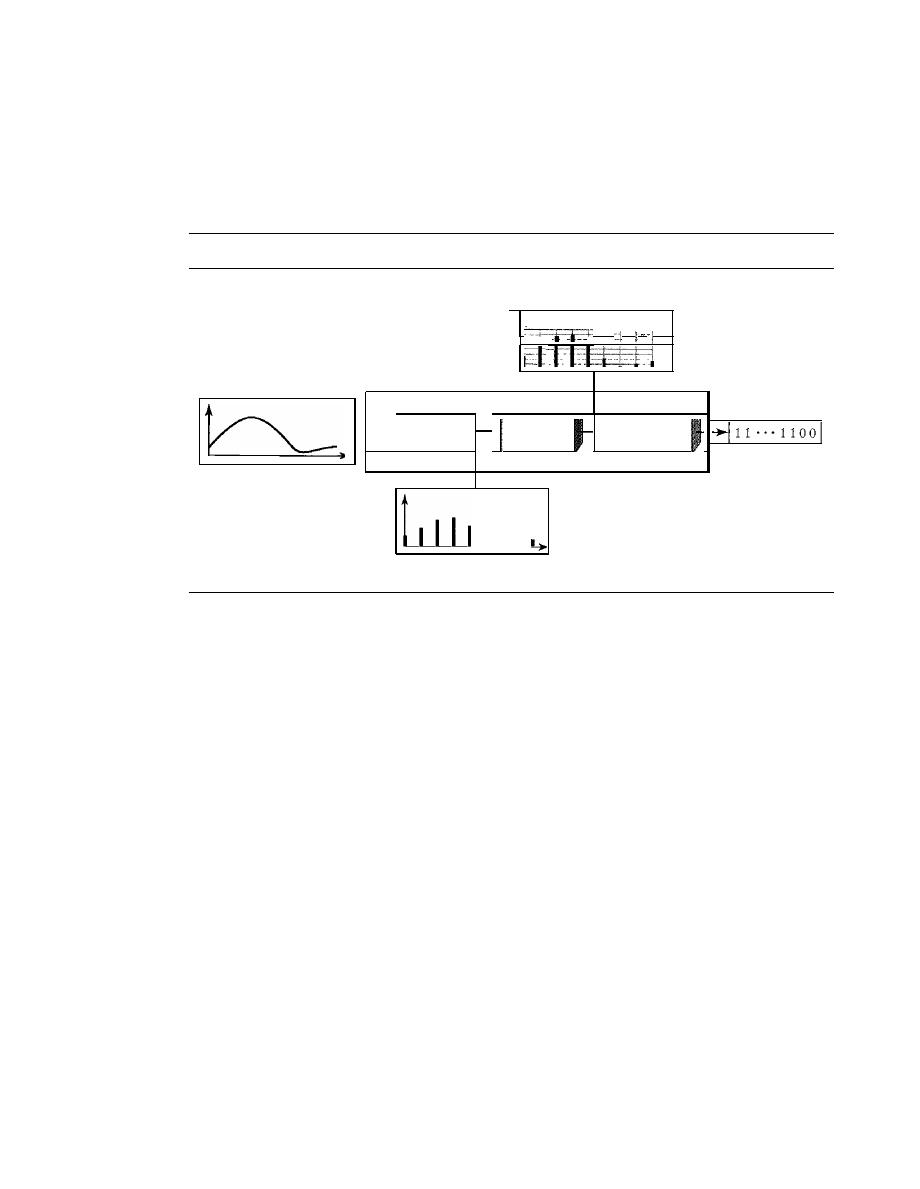
SECTION
4.2
ANALOG-TO-DIGITAL CONVERSION
121
Pulse Code Modulation (PCM)
The most common technique to change an analog signal to digital data (digitization)
is called pulse code modulation (PCM). A PCM encoder has three processes, as shown
in Figure 4.21.
Figure 4.21
Components of PCM encoder
Quantized signal
!
peM
encoder
H
Sampling;
Quantizing
Encoding
Digital data
Analog signal
I
.
I
PAM signal
1.
The analog signal is sampled.
2. The sampled signal is quantized.
3. The quantized values are encoded as streams of bits.
Sampling
The first step in PCM is sampling. The analog signal is sampled every
T
s
s, where
T
s
is
the sample interval or period. The inverse of the sampling interval is called the sam-
pling rate or sampling frequency and denoted by
is,
where
is =
IIT
s'
There are three
sampling methods-ideal, natural, and flat-top-as shown in Figure 4.22.
In ideal sampling, pulses from the analog signal are sampled. This is an ideal sam-
pling method and cannot be easily implemented. In natural sampling, a high-speed
switch is turned on for only the small period of time when the sampling occurs. The
result is a sequence of samples that retains the shape of the analog signal. The most
common sampling method, called sample and hold, however, creates flat-top samples
by using a circuit.
The sampling process is sometimes referred to as pulse amplitude modulation
(PAM). We need to remember, however, that the result is still an analog signal with
nonintegral values.
Sampling Rate
One important consideration is the sampling rate or frequency. What
are the restrictions on
T
s
?
This question was elegantly answered by Nyquist. According
to the Nyquist theorem, to reproduce the original analog signal, one necessary condition
is that the sampling rate be at least twice the highest frequency in the original signal.
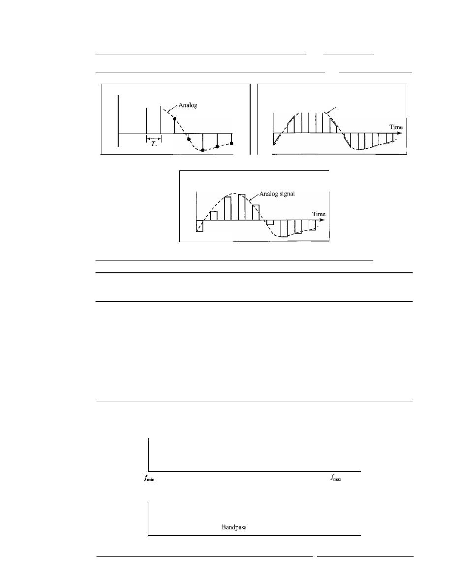
122
CHAPTER
4
DIGITAL TRANSMISSION
Figure 4.22
Three different sampling methods for PCM
Amplitude
Amplitude
signal
"
s
a. Ideal sampling
Amplitude
c. Flat-top sampling
Time
b. Natural sampling
Analog signal
According to the Nyquist theorem, the sampling rate must be
at least 2 times the highest frequency contained in the signal.
We need to elaborate on the theorem at this point. First, we can sample a signal
only if the signal is band-limited. In other words, a signal with an infinite bandwidth
cannot be sampled. Second, the sampling rate must be at least 2 times the highest fre-
quency, not the bandwidth. If the analog signal is low-pass, the bandwidth and the
highest frequency are the same value.
If
the analog signal is bandpass, the bandwidth
value is lower than the value of the maximum frequency. Figure 4.23 shows the value
of the sampling rate for two types of signals.
Figure 4.23
Nyquist sampling rate for low-pass and bandpass signals
- - - - - - - - - - - - - - - - - - - - - - - - - - - - - - - - - - - - -
Amplitude
Nyquist rate
=
2 x
fm"x
Low-pass signal
Amplitude
o
Nyquist rate
=
2 x
fmax
signal
f
min
Frequency
Frequency
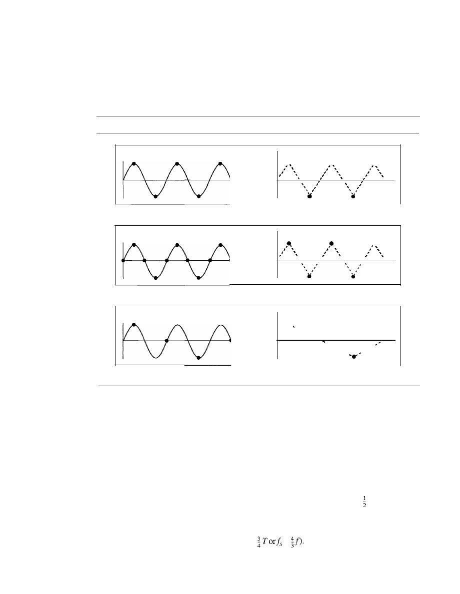
SECTION
4.2
ANALOG-TO-DIGITAL CONVERSION
123
Example 4.6
For an intuitive example of the Nyquist theorem, let us sample a simple sine wave at three sam-
pling rates: fs
=
4f
(2 times the Nyquist rate )'/s
=
2f
(Nyquist rate), and f s
=
f
(one-half the
Nyquist rate). Figure 4.24 shows the sampling and the subsequent recovery of the signal.
Figure 4.24
Recovery of a sampled sine wave for different sampling rates
a. Nyquist rate sampling:f
s
=
2f
b. Oversampling:f
s
=
4f
•
•
•
•
c. Undersampling:
f
s
=
f
.....
It can be seen that sampling at the Nyquist rate can create a good approximation of the orig-
inal sine wave (part a). Oversampling in part b can also create the same approximation, but it is
redundant and unnecessary. Sampling below the Nyquist rate (part c) does not produce a signal
that looks like the original sine wave.
Example 4.7
As an interesting example, let us see what happens if we sample a periodic event such as the revolu-
tion of a hand of a clock. The second hand of a clock has a period of 60 s. According to the Nyquist
theorem, we need to sample the hand (take and send a picture) every 30 s (T
s
=
Tor f
s
=
2f).
In
Figure 4.25a, the sample points, in order, are 12, 6, 12, 6, 12, and 6. The receiver of the samples
cannot tell if the clock is moving forward or backward. In part b, we sample at double the Nyquist
rate (every 15 s). The sample points, in order, are 12,3,6, 9, and 12. The clock is moving forward.
In part c, we sample below the Nyquist rate
(T
s
=
=
The sample points, in order, are 12,
9,6,3, and 12. Although the clock is moving forward, the receiver thinks that the clock is moving
backward.
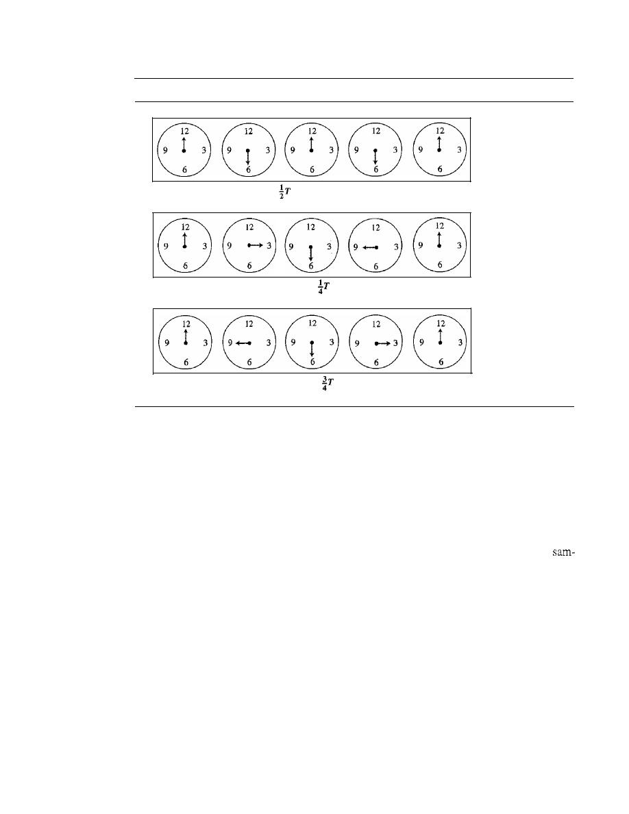
124
CHAPTER
4
DIGITAL TRANSMISSION
Figure 4.25
Sampling of a clock with only one hand
a. Sampling at Nyquist rate:
T
s
=
b. Oversampling (above Nyquist rate):
T
s
=
c. Undersampling (below Nyquist rate):
T
s
=
Samples can mean that
the clock is moving
either forward or
backward.
(12-6-12-6-12)
Samples show clock
is moving forward.
(12·3-6-9-12)
Samples show clock
is moving backward.
(12-9-6-3-12)
Example 4.8
An example related to Example 4.7 is the seemingly backward rotation of the wheels of a forward-
moving car in a movie. This can be explained by undersampling. A movie is filmed at 24 frames
per second. If a wheel is rotating more than 12 times per second, the undersampling creates the
impression of a backward rotation.
Example 4.9
Telephone companies digitize voice by assuming a maximum frequency of 4000 Hz. The
pling rate therefore is 8000 samples per second.
Example 4.10
A complex low-pass signal has a bandwidth of 200 kHz. What is the minimum sampling rate for
this signal?
Solution
The bandwidth of a low-pass signal is between 0 andj, where
f
is the maximum frequency in the
signal. Therefore, we can sample this signal at 2 times the highest frequency (200 kHz). The sam-
pling rate is therefore 400,000 samples per second.
Example
4.1
J
A complex bandpass signal has a bandwidth of 200 kHz. What is the minimum sampling rate for
this signal?
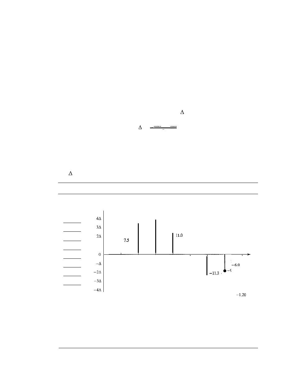
SECTION
4.2
ANALOG-TO-DIGITAL CONVERSION
125
Solution
We cannot find the minimum sampling rate in this case because we do not know where the band-
width starts or ends. We do not know the maximum frequency in the signal.
Quantization
The result of sampling is a series of pulses with amplitude values between the maxi-
mum and minimum amplitudes of the signal. The set of amplitudes can be infinite with
nonintegral values between the two limits. These values cannot be used in the encoding
process. The following are the steps in quantization:
1. We assume that the original analog signal has instantaneous amplitudes between
V
min
and V
max'
2. We divide the range into
L
zones, each of height
(delta).
V
max -
V
rnin
=
L
3. We assign quantized values of 0 to
L -
I to the midpoint of each zone.
4. We approximate the value of the sample amplitude to the quantized values.
As a simple example, assume that we have a sampled signal and the sample ampli-
tudes are between
-20 and +20
V.
We decide to have eight levels
(L
=
8). This means
that
=
5 V. Figure 4.26 shows this example.
Figure 4.26
Quantization and encoding of a sampled signal
Quantization
Normalized
codes
amplitude
7
19.7
5
-5.5
1
Time
-9.4
-6.1
2
Normalized
-1.22
PAM values
Normalized
-1.50
quantized values
1.50
3.24
3.94
2.20
-1.10
-2.26
-1.88
1.50
3.50
3.50
2.50
-1.50
-2.50
-1.50
-1.50
Normalized
-0.38
error
o
+0.26
-0.44
+0.30
-0.40
-0.24
+0.38
-0.30
Quantization code
2
5
7
7
6
2
2
2
Encoded words
010
101
111
111
110
010
001
010
ow

126
CHAPTER
4
DIGITAL TRANSMISSION
We have shown only nine samples using ideal sampling (for simplicity). The
value at the top of each sample in the graph shows the actual amplitude. In the chart,
the first row is the normalized value for each sample (actual
The quan-
tization process selects the quantization value from the middle of each zone. This
means that the normalized quantized values (second row) are different from the nor-
malized amplitudes. The difference is called the normalized error (third row). The
fourth row is the quantization code for each sample based on the quantization levels
at the left of the graph. The encoded words (fifth row) are the final products of the
conversion.
Quantization Levels
In the previous example, we showed eight quantization levels.
The choice of
L,
the number of levels, depends on the range of the amplitudes of the
analog signal and how accurately we need to recover the signal.
If
the amplitude of a
signal fluctuates between two values only, we need only two levels; if the signal, like
voice, has many amplitude values, we need more quantization levels. In audio digitiz-
ing,
L
is normally chosen to be 256; in video
it
is normally thousands. Choosing
lower values of
L
increases the quantization error if there is a lot of fluctuation in the
signal.
Quantization Error
One important issue is the error created in the quantization pro-
cess. (Later, we will see how this affects high-speed modems.) Quantization is an
approximation process. The input values to the quantizer are the real values; the output
values are the approximated values. The output values are chosen to be the middle
value in the zone. If the input value is also at the middle of the zone, there is no quanti-
zation error; otherwise, there is an error. In the previous example, the normalized
amplitude of the third sample is 3.24, but the normalized quantized value is 3.50. This
means that there is an error of +0.26. The value of the error for any sample is less than
In other words, we have
error
The quantization error changes the signal-to-noise ratio of the signal, which in turn
reduces the upper limit capacity according to Shannon.
It can be proven that the contribution of the quantization error to the SNR
dB
of
the signal depends on the number of quantization levels
L,
or the bits per sample
nb'
as
shown in the following formula:
SNR
dB
=
6.02nb
+
1.76 dB
Example 4.12
What is the SNR
dB
in the example of Figure 4.26?
Solution
We can use the formula to find the quantization. We have eight levels and 3 bits per sample, so
SNR
dB
=
6.02(3)
+
1.76
=
19.82 dB. Increasing the number of levels increases the SNR.
Example 4.13
A telephone subscriber line must have an
above 40. What is the minimum number of bits
per sample?

SECTION
ANALOG-TO-DIGITAL CONVERSION
127
Solution
We can calculate the number of bits as
6.02nb
+
1.76:::: 40
n:::: 6.35
Telephone companies usually assign 7 or 8 bits per sample.
Uniform Versus Nonuniform Quantization
For many applications, the distribu-
tion of the instantaneous amplitudes in the analog signal is not uniform. Changes in
amplitude often occur more frequently in the lower amplitudes than in the higher
ones. For these types of applications it is better to use nonuniform zones. In other
words, the height of
is not fixed; it is greater near the lower amplitudes and less
near the higher amplitudes. Nonuniform quantization can also be achieved by using a
process called companding and expanding. The signal is companded at the sender
before conversion; it is expanded at the receiver after conversion. Companding means
reducing the instantaneous voltage amplitude for large values; expanding is the oppo-
site process. Companding gives greater weight to strong signals and less weight to
weak ones. It has been proved that nonuniform quantization effectively reduces the
SNR
dB
of quantization.
Encoding
The last step in PCM is encoding. After each sample is quantized and the number of
bits per sample is decided, each sample can be changed to an llb-bit code word. In Fig-
ure 4.26 the encoded words are shown in the last row. A quantization code of 2 is
encoded as 010; 5 is encoded as 101; and so on. Note that the number of bits for each
sample is determined from the number of quantization levels. If the number of quanti-
zation levels is
L,
the number of bits is
llb
=
log2
L.
In our example
L
is 8 and
llb
is
therefore 3. The bit rate can be found from the formula
Bit
rate :::: sampling rate x number of bits per sample::::
x
nb
Example 4.14
We want to digitize the human voice. What is the bit rate, assuming 8 bits per sample?
Solution
The human voice normally contains frequencies from 0 to 4000 Hz. So the sampling rate and bit
rate are calculated as follows:
Sampling rate :::: 4000 x 2 :::: 8000 samples/s
Bit rate
8000 x 8 :::: 64,000 bps
64 kbps
Original Signal Recovery
The recovery of the original signal requires the PCM decoder. The decoder first uses
circuitry to convert the code words into a pulse that holds the amplitude until the next
pulse. After the staircase signal is completed, it is passed through a low-pass filter to
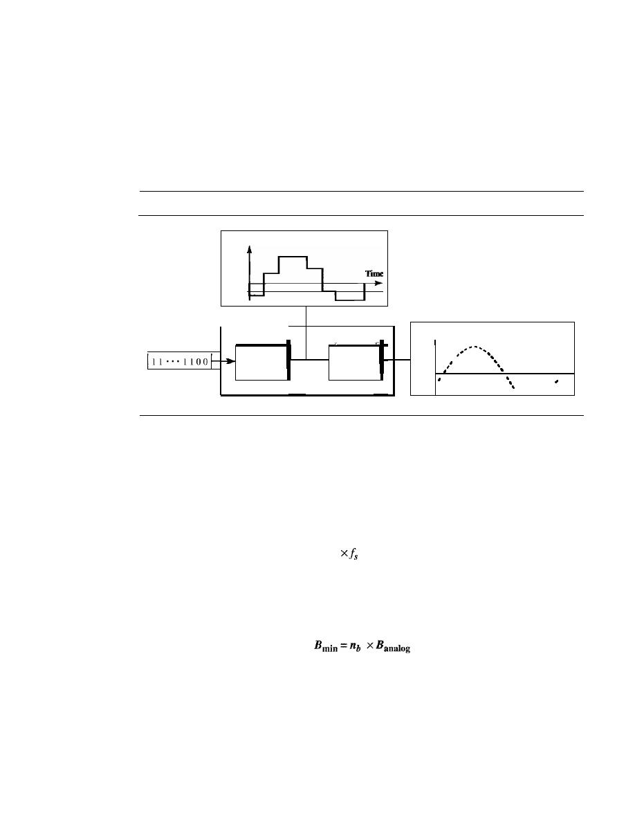
128
CHAPTER
4
DIGITAL TRANSMISSION
smooth the staircase signal into an analog signal. The filter has the same cutoff fre-
quency as the original signal at the sender.
If
the signal has been sampled at (or
greater than) the Nyquist sampling rate and if there are enough quantization levels,
the original signal will be recreated. Note that the maximum and minimum values of
the original signal can be achieved by using amplification. Figure 4.27 shows the
simplified process.
Figure 4.27
Components of a PCM decoder
Amplitude
PCM decoder
Amplitude
Analog signal
Make and
Low-pass
connect
Time
filter
samples
Digital data
..
-.-
..
,
PCM Bandwidth
Suppose we are given the bandwidth of a low-pass analog signal.
If
we then digitize the
signal, what is the new minimum bandwidth of the channel that can pass this digitized
signal? We have said that the minimum bandwidth of a line-encoded signal is
B
min
=
ex
N
x
(lIr).
We substitute the value of
N
in this formula:
1 1 1
B
min
=
c
x
N
x -
=
c
X
nb
x -
=
c x
nb
x 2 x Banalog
x -
r
r
r
When
lIr
=
I (for a NRZ or bipolar signal) and c
=
(12)
(the average situation), the
minimum bandwidth is
This means the minimum bandwidth of the digital signal is
nb
times greater than the
bandwidth of the analog signal. This is the price we pay for digitization.
Example 4.15
We have a low-pass analog signal of 4 kHz. If we send the analog signal, we need a channel with
a minimum bandwidth of 4 kHz. If we digitize the signal and send 8 bits per sample, we need a
channel with a minimum bandwidth of 8
X
4 kHz
=
32 kHz.
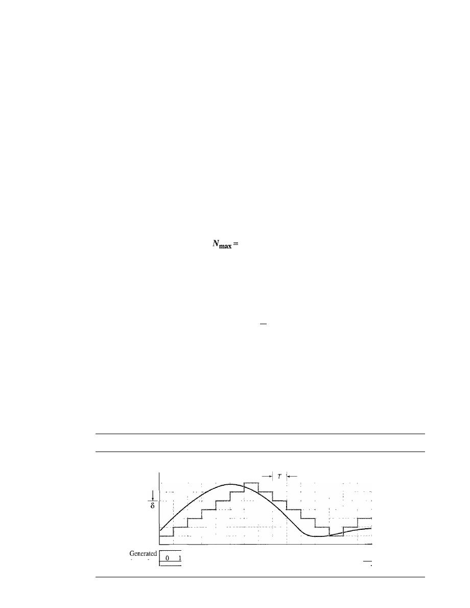
SECTION
4.2
ANALOG-TO-DIGITAL CONVERSION
129
Maximum Data Rate of a Channel
In Chapter 3, we discussed the Nyquist theorem which gives the data rate of a channel
as
N
max
=
2 x
B
x log
2
L.
We can deduce this rate from the Nyquist sampling theorem
by using the following arguments.
1. We assume that the available channel is low-pass with bandwidth B.
2.
We assume that the digital signal we want to send has
L
levels, where each level is
a signal element. This means
r
=
1/10g
2
L.
3. We first pass the digital signal through a low-pass filter to cut off the frequencies
above
B
Hz.
4. We treat the resulting signal as an analog signal and sample it at 2 x
B
samples per
second and quantize it using L levels. Additional quantization levels are useless
because the signal originally had
L
levels.
S. The resulting bit rate is N
=
fs x
nb
=
2 x
B x log2
L.
This is the maximum band-
width; if the case factor
c
increases, the data rate is reduced.
2
x
B
x
logzL bps
Minimum Required Bandwidth
The previous argument can give us the minimum bandwidth if the data rate and the
number of signal levels are fixed. We can say
B .
=
N
Hz
mm
2xlog
z
L
Delta Modulation
(DM)
PCM is a very complex technique. Other techniques have been developed to reduce
the complexity of PCM. The simplest is
delta modulation.
PCM finds the value of the
signal amplitude for each sample; DM finds the change from the previous sample. Fig-
ure 4.28 shows the process. Note that there are no code words here; bits are sent one
after another.
Figure 4.28
The process of delta modulation
Amplitude
T
1_1
Time
bmary data
0
0
0
0
0
0
130
CHAPTER
4
DIGITAL TRANSMISSION
Modulator
The modulator is used at the sender site to create a stream of bits from an analog signal.
The process records the small positive or negative changes, called delta
If
the delta is
positive, the process records a I; if it is negative, the process records a O. However, the
process needs a base against which the analog signal is compared. The modulator
builds a second signal that resembles a staircase. Finding the change is then reduced to
comparing the input signal with the gradually made staircase signal. Figure 4.29 shows
a diagram of the process.
Figure 4.29
Delta modulation components
OM modulator
Digital data
Analog signal
t
t
I I •.. I 100
ompraor
The modulator, at each sampling interval, compares the value of the analog signal
with the last value of the staircase signal.
If
the amplitude of the analog signal is larger,
the next bit in the digital data is 1; otherwise, it is O. The output of the comparator, how-
ever, also makes the staircase itself. If the next bit is I, the staircase maker moves the
last point of the staircase signal
up; it the next bit is 0, it moves it
down. Note that we
need a delay unit to hold the staircase function for a period between two comparisons.
Demodulator
The demodulator takes the digital data and, using the staircase maker and the delay
unit, creates the analog signal. The created analog signal, however, needs to pass
through a low-pass filter for smoothing. Figure 4.30 shows the schematic diagram.
Figure 4.30
Delta demodulation components
OM demodulator
11"'1100
Digital data
Analog signal
SECTION
4.3
TRANSMISSION MODES
131
Adaptive
A better performance can be achieved if the value of
is not fixed. In
adaptive delta
modulation,
the value of
changes according to the amplitude of the analog signal.
Quantization Error
It
is obvious that DM is not perfect. Quantization error is always introduced in the pro-
cess. The quantization error of DM, however, is much less than that for PCM.
4.3
TRANSMISSION MODES
Of primary concern when we are considering the transmission of data from one device
to another is the wiring, and of primary concern when we are considering the wiring is
the data stream. Do we send 1 bit at a time; or do we group bits into larger groups and,
if so, how? The transmission of binary data across a link can be accomplished in either
parallel or serial mode. In parallel mode, multiple bits are sent with each clock tick.
In serial mode, 1 bit is sent with each clock tick. While there is only one way to send
parallel data, there are three subclasses of serial transmission: asynchronous, synchro-
nous, and isochronous (see Figure 4.31).
Figure 4.31
Data transmission and modes
Data transmission
Parallel Transmission
Binary data, consisting of Is and Os, may be organized into groups of
n
bits each.
Computers produce and consume data in groups of bits much as we conceive of and use
spoken language in the form of words rather than letters. By grouping, we can send
data n bits at a time instead of 1. This is called
parallel transmission.
The mechanism for parallel transmission is a conceptually simple one: Use
n
wires
to send n bits at one time. That way each bit has its own wire, and all n bits of one
group can be transmitted with each clock tick from one device to another. Figure 4.32
shows how parallel transmission works for
n
=
8. Typically, the eight wires are bundled
in a cable with a connector at each end.
The advantage of parallel transmission is speed. All else being equal, parallel
transmission can increase the transfer speed by a factor of n over serial transmission.
132
CHAPTER
4
DIGITAL TRANSMISSION
Figure 4.32
Parallel transmission
The 8 bits are sent together
I
v
\
I
\
f
I
\
1
1
I
Sender
I
v
I
Receiver
I
v
j
v
I
\
\
I
/
We need eight lines
But there is a significant disadvantage: cost. Parallel transmission requires n communi-
cation lines (wires in the example) just to transmit the data stream. Because this is
expensive, parallel transmission is usually limited to short distances.
Serial Transmission
In
serial transmission
one bit follows another, so we need only one communica-
tion channel rather than n to transmit data between two communicating devices (see
Figure 4.33).
Figure 4.33
Serial transmission
We need only
one line (wire).
o
1
1
Sender
0
o
o
1
o
The 8 bits are sent
one after another.
o
1
o
0 0 0 1 0
1
Receiver
o
1
o
Parallel/serial
converter
Serial/parallel
converter
The advantage of serial over parallel transmission is that with only one communi-
cation channel, serial transmission reduces the cost of transmission over parallel by
roughly a factor of n.
Since communication within devices is parallel, conversion devices are required at
the interface between the sender and the line (parallel-to-serial) and between the line
and the receiver (serial-to-parallel).
Serial transmission occurs in one of three ways: asynchronous, synchronous, and
isochronous.

SECTION
4.3
TRANSMISSION MODES
133
Asynchronous Transmission
Asynchronous transmission is so named because the timing of a signal is unimportant.
Instead, information is received and translated by agreed upon patterns. As long as those
patterns are followed, the receiving device can retrieve the information without regard
to the rhythm in which it is sent. Patterns are based on grouping the bit stream into
bytes. Each group, usually 8 bits, is sent along the link as a unit. The sending system
handles each group independently, relaying it to the link whenever ready, without regard
to a timer.
Without synchronization, the receiver cannot use timing to predict when the next
group will arrive. To alert the receiver to the arrival of a new group, therefore, an extra
bit is added to the beginning of each byte. This bit, usually a
0, is called the start bit.
To let the receiver know that the byte is finished, 1 or more additional bits are appended
to the end of the byte. These bits, usually
I s, are called stop bits. By this method, each
byte is increased in size to at least 10 bits, of which 8 bits is information and 2 bits or
more are signals to the receiver. In addition, the transmission of each byte may then be
followed by a gap of varying duration. This gap can be represented either by an idle
channel or by a stream of additional stop bits.
In asynchronous transmission, we send 1 start bit (0) at the beginning and 1 or more
stop bits (Is) at the end of each byte. There may be a gap between each byte.
The start and stop bits and the gap alert the receiver to the beginning and end of
each byte and allow it to synchronize with the data stream. This mechanism is called
asynchronous
because, at the byte level, the sender and receiver do not have to be syn-
chronized. But within each byte, the receiver must still be synchronized with the
incoming bit stream. That is, some synchronization is required, but only for the
tion of a single byte. The receiving device resynchronizes at the onset of each new byte.
When the receiver detects a start bit, it sets a timer and begins counting bits as they
come in. After
n
bits, the receiver looks for a stop bit. As soon as it detects the stop bit,
it waits until it detects the next start bit.
Asynchronous here means "asynchronous at the byte
but the bits are still synchronized; their durations are the same.
Figure 4.34 is a schematic illustration of asynchronous transmission. In this exam-
ple, the start bits are as, the stop bits are 1s, and the gap is represented by an idle line
rather than by additional stop bits.
The addition of stop and start bits and the insertion of gaps into the bit stream
make asynchronous transmission slower than forms of transmission that can operate
without the addition of control information. But it is cheap and effective, two advan-
tages that make it an attractive choice for situations such as low-speed communication.
For example, the connection of a keyboard to a computer is a natural application for
asynchronous transmission. A user types only one character at a time, types extremely
slowly in data processing terms, and leaves unpredictable gaps of time between each
character.
134
CHAPTER
4
DIGITAL TRANSMISSION
Figure 4.34
Asynchronous transmission
Direction of flow
bit
0
Sender
01 101
I
0
I
1111101 1
000101 1 1
11 11 1
Gaps between
data units
Receiver
Synchronous Transmission
In
synchronous transmission,
the bit stream is combined into longer "frames," which
may contain multiple bytes. Each byte, however, is introduced onto the transmission
link without a gap between it and the next one.
It
is left to the receiver to separate the
bit stream into bytes for decoding purposes. In other words, data are transmitted as an
unbroken string of 1s and Os, and the receiver separates that string into the bytes, or
characters, it needs to reconstruct the information.
In synchronous transmission, we send bits one after another without start or stop
bits or gaps.
It
is the responsibility of the receiver to group the bits.
Figure 4.35 gives a schematic illustration of synchronous transmission. We have
drawn in the divisions between bytes. In reality, those divisions do not exist; the sender
puts its data onto the line as one long string. If the sender wishes to send data in separate
bursts, the gaps between bursts must be filled with a special sequence of Os and Is that
means idle. The receiver counts the bits as they arrive and groups them in 8-bit units.
Figure 4.35
Synchronous transmission
Direction of flow
Sender
1 1
0 1 I I
I
Frame
111111011111110110
I···
j
111101111
Frame
1,----tReceiver
11 1 1 1
Without gaps and start and stop bits, there is no built-in mechanism to help the
receiving device adjust its bit synchronization midstream. Timing becomes very impor-
tant, therefore, because the accuracy of the received information is completely dependent
on the ability of the receiving device to keep an accurate count of the bits as they come in.

SECTION
4.5
KEY TERMS
135
The advantage of synchronous transmission is speed. With no extra bits or gaps to
introduce at the sending end and remove at the receiving end, and, by extension, with
fewer bits to move across the link, synchronous transmission is faster than
nous transmission. For this reason, it is more useful for high-speed applications such as
the transmission of data from one computer to another. Byte synchronization is accom-
plished in the data link layer.
We need to emphasize one point here. Although there is no gap between characters
in synchronous serial transmission, there may be uneven gaps between frames.
Isochronous
In real-time audio and video, in which uneven delays between frames are not accept-
able, synchronous transmission fails. For example, TV images are broadcast at the rate
of 30 images per second; they must be viewed at the same rate. If each image is sent
by using one or more frames, there should be no delays between frames. For this type
of application, synchronization between characters is not enough; the entire stream of
bits must be synchronized. The isochronous transmission guarantees that the data
arrive at a fixed rate.
4.4
RECOMMENDED READING
For more details about subjects discussed in this chapter, we recommend the following
books. The items in brackets [...] refer to the reference list at the end of the text.
Books
Digital to digital conversion is discussed in Chapter 7 of [Pea92], Chapter 3 of
[CouOl], and Section 5.1 of [Sta04]. Sampling is discussed in Chapters 15, 16, 17, and
18 of [Pea92], Chapter 3 of [CouO!], and Section 5.3 of [Sta04]. [Hsu03] gives a good
mathematical approach to modulation and sampling. More advanced materials can be
found in [Ber96].
4.5
KEY TERMS
adaptive delta modulation
alternate mark inversion (AMI)
analog-to-digital conversion
asynchronous transmission
baseline
baseline wandering
baud rate
biphase
bipolar
bipolar with 8-zero substitution (B8ZS)
bit rate
block coding
companding and expanding
data element
data rate
DC component
delta modulation (DM)
differential Manchester
digital-to-digital conversion
digitization

136
CHAPTER
4
DIGITAL TRANSMISSION
eight binary/ten binary (8B/lOB)
eight-binary, six-ternary (8B6T)
four binary/five binary (4B/5B)
four dimensional, five-level pulse
amplitude modulation (4D-PAM5)
high-density bipolar 3-zero (HDB3)
isochronous transmission
line coding
Manchester
modulation rate
multilevel binary
multiline transmission, 3 level (MLT-3)
nonreturn to zero (NRZ)
nonreturn to zero, invert (NRZ-I)
nonreturn to zero, level (NRZ-L)
Nyquist theorem
parallel transmission
polar
pseudoternary
pulse amplitude modulation (PAM)
pulse code modulation (PCM)
pulse rate
quantization
quantization error
return to zero (RZ)
sampling
sampling rate
scrambling
self-synchronizing
serial transmission
signal element
signal rate
start bit
stop bit
synchronous transmission
transmission mode
two-binary, one quaternary (2B
I
Q)
unipolar
4.6
SUMMARY
o
Digital-to-digital conversion involves three techniques: line coding, block coding,
and scrambling.
o
Line coding is the process of converting digital data to a digital signal.
o
We can roughly divide line coding schemes into five broad categories: unipolar,
polar, bipolar, multilevel, and multitransition.
o
Block coding provides redundancy to ensure synchronization and inherent error
detection. Block coding is normally referred to as mB/nB coding; it replaces each
m-bit group with an n-bit
group.
o
Scrambling provides synchronization without increasing the number of bits. Two
common scrambling techniques are B8ZS and HDB3.
o
The most common technique to change an analog signal to digital data (digitiza-
tion) is called pulse code modulation (PCM).
o
The first step in PCM is sampling. The analog signal is sampled every Ts s, where Ts
is the sample interval or period. The inverse of the sampling interval is called the
sampling rate
or sampling frequency and denoted by fs, where fs
=
lITs.
There are
three sampling methods-ideal, natural, and flat-top.
o
According to the Nyquist theorem, to reproduce the original analog signal, one
necessary condition is that the sampling rate be at least twice the highest frequency
in the original signal.

SECTION
4.7
PRACTICE SET
137
o
Other sampling techniques have been developed to reduce the complexity of PCM.
The simplest is
delta modulation. PCM finds the value of the signal amplitude for
each sample; DM finds the change from the previous sample.
o
While there is only one way to send parallel data, there are three subclasses of
serial transmission: asynchronous, synchronous, and isochronous.
o
In asynchronous transmission, we send 1 start bit (0) at the beginning and 1 or
more stop bits (1 s) at the end of each byte.
o
In synchronous transmission, we send bits one after another without start or stop
bits or gaps.
It
is the responsibility of the receiver to group the bits.
o
The isochronous mode provides synchronized for the entire stream of bits must. In
other words, it guarantees that the data arrive at a fixed rate.
4.7
PRACTICE SET
Review Questions
1. List three techniques of digital-to-digital conversion.
2. Distinguish between a signal element and a data element.
3. Distinguish between data rate and signal rate.
4. Define baseline wandering and its effect on digital transmission.
5. Define a DC component and its effect on digital transmission.
6. Define the characteristics of a self-synchronizing signal.
7. List five line coding schemes discussed in this book.
8. Define block coding and give its purpose.
9. Define scrambling and give its purpose.
10. Compare and contrast PCM and DM.
11. What are the differences between parallel and serial transmission?
12. List three different techniques in serial transmission and explain the differences.
Exercises
13. Calculate the value of the signal rate for each case in Figure 4.2 if the data rate is
1 Mbps and c
=
1/2.
14. In a digital transmission, the sender clock is 0.2 percent faster than the receiver clock.
How many extra bits per second does the sender send if the data rate is 1 Mbps?
15.
Draw the graph of the NRZ-L scheme using each of the following data streams,
assuming that the last signa11evel has been positive. From the graphs, guess the
bandwidth for this scheme using the average number of changes in the signal level.
Compare your guess with the corresp.onding entry in Table 4.1.
a. 00000000
b. 11111111
c. 01010101
d. 00110011
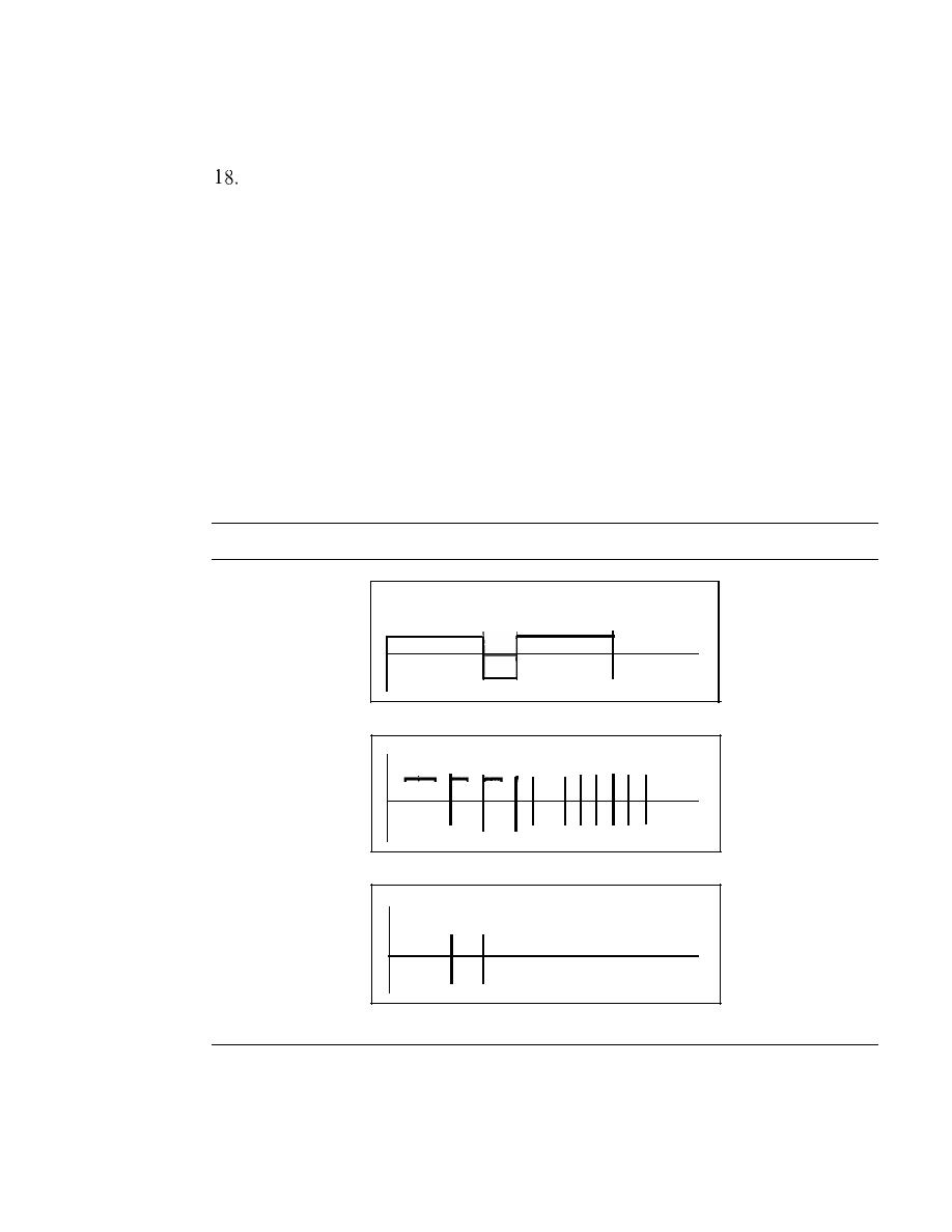
138
CHAPTER
4
DIGITAL TRANSMISSION
16. Repeat Exercise 15 for the NRZ-I scheme.
17. Repeat Exercise 15 for the Manchester scheme.
Repeat Exercise 15 for the differential Manchester scheme.
19. Repeat Exercise 15 for the 2B 1
Q
scheme, but use the following data streams.
a. 0000000000000000
b. 1111111111111111
c. 0101010101010101
d. 0011001100110011
20. Repeat Exercise 15 for the MLT-3 scheme, but use the following data streams.
a. 00000000
b. 11111111
c. 01010101
d. 00011000
21. Find the 8-bit data stream for each case depicted in Figure 4.36.
Figure 4.36
Exercise 21
t
Time
a. NRZ-I
Time
b. differential Manchester
Time
c.AMI
22. An NRZ-I signal has a data rate of 100 Kbps. Using Figure 4.6, calculate the value
of the normalized energy (P) for frequencies at 0 Hz, 50 KHz, and 100 KHz.
23. A Manchester signal has a data rate of 100 Kbps. Using Figure 4.8, calculate the
value of the normalized energy (P) for frequencies at 0 Hz, 50 KHz, 100 KHz.

SECTION
4. 7
PRACTICE SET
139
24. The input stream to a 4B/5B block encoder is 0100 0000 0000 0000 0000 OOOI.
Answer the following questions:
a.
What is the output stream?
b. What is the length of the longest consecutive sequence of Os in the input?
c.
What is the length of the longest consecutive sequence of Os in the output?
25. How many invalid (unused) code sequences can we have in 5B/6B encoding? How
many in 3B/4B encoding?
26. What is the result of scrambling the sequence 11100000000000 using one of the
following scrambling techniques? Assume that the last non-zero signal level has
been positive.
a.
B8ZS
b. HDB3 (The number of nonzero pules is odd after the last substitution)
27.
What is the Nyquist sampling rate for each of the following signals?
a.
A low-pass signal with bandwidth of 200 KHz?
b. A band-pass signal with bandwidth of 200 KHz if the lowest frequency is
100 KHz?
28.
We have sampled a low-pass signal with a bandwidth of 200 KHz using 1024 levels
of quantization.
a. Calculate the bit rate of the digitized signal.
b. Calculate the SNR
dB
for this signal.
c.
Calculate the PCM bandwidth of this signal.
29. What is the maximum data rate of a channel with a bandwidth of 200 KHz if we
use four levels of digital signaling.
30. An analog signal has a bandwidth of 20 KHz. If we sample this signal and send it
through a 30 Kbps channel what is the SNR
dB
?
31.
We have a baseband channel with a I-MHz bandwidth. What is the data rate for
this channel if we use one of the following line coding schemes?
a.
NRZ-L
b. Manchester
c.
MLT-3
d.
2B1Q
32. We want to transmit 1000 characters with each character encoded as 8 bits.
a. Find the number of transmitted bits for synchronous transmission.
b. Find the number of transmitted bits for asynchronous transmission.
c. Find the redundancy percent in each case.

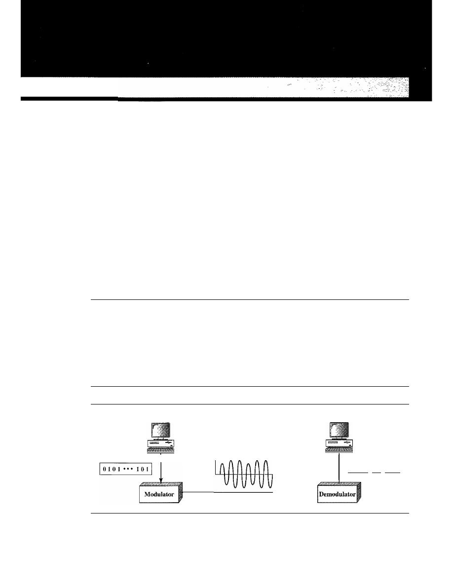
CHAPTERS
Analog Transmission
In Chapter 3, we discussed the advantages and disadvantages of digital and analog trans-
mission. We saw that while digital transmission is very desirable, a low-pass channel is
needed. We also saw that analog transmission is the only choice if we have a bandpass
channel. Digital transmission was discussed in Chapter 4; we discuss analog transmis-
sion in this chapter.
Converting digital data
to
a bandpass analog signal.is traditionally called digital-
to-analog conversion. Converting a low-pass analog signal to a bandpass analog signal
is traditionally called analog-to-analog conversion. In this chapter, we discuss these two
types of conversions.
5.1
DIGITAL-TO-ANALOG CONVERSION
Digital-to-analog conversion is the process of changing one of the characteristics of
an analog signal based on the information in digital data. Figure 5.1 shows the rela-
tionship between the digital information, the digital-to-analog modulating process,
and the resultant analog signal.
Figure 5.1
Digital-to-analog conversion
Digital data
Sender
Analog signal
Link
Receiver
Digital data
1°101 ... 1011
141
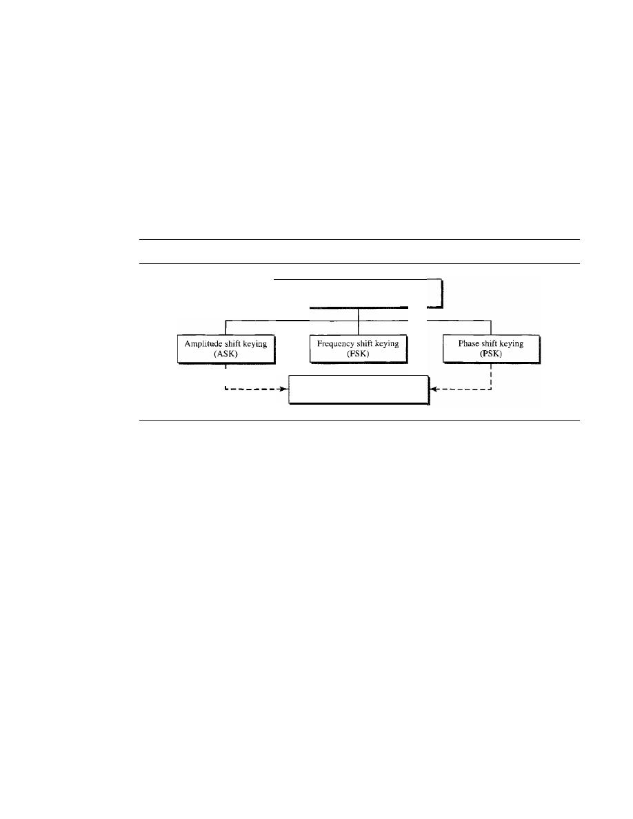
142
CHAPTER 5
ANALOG TRANSMISSION
As discussed in Chapter 3, a sine wave is defined by three characteristics: amplitude,
frequency, and phase. When we vary anyone of these characteristics, we create a differ-
ent version of that wave. So, by changing one characteristic of a simple electric signal, we
can use it to represent digital data. Any of the three characteristics can be altered in this
way, giving us at least three mechanisms for modulating digital data into an analog signal:
amplitude shift keying (ASK), frequency shift keying (FSK), and phase shift keying
(PSK). In addition, there is a fourth (and better) mechanism that combines changing both
the amplitude and phase, called quadrature amplitude modulation (QAM). QAM
is the most efficient of these options and is the mechanism commonly used today (see
Figure 5.2).
Figure 5.2
Types of digital-to-analog conversion
Digital-to-analog
conversion
Quadrature amplitude modulation
(QAM)
Aspects of Digital-to-Analog Conversion
Before we discuss specific methods of digital-to-analog modulation, two basic issues
must be reviewed: bit and baud rates and the carrier signal.
Data Element Versus Signal Element
In Chapter 4, we discussed the concept of the data element versus the signal element.
We defined a data element as the smallest piece of information to be exchanged, the
bit. We also defined a signal element as the smallest unit of a signal that is constant.
Although we continue to use the same terms in this chapter, we will see that the nature
of the signal element is a little bit different in analog transmission.
Data Rate Versus Signal Rate
We can define the data rate (bit rate) and the signal rate (baud rate) as we did for digital
transmission. The relationship between them is
S=Nx!
baud
r
where
N
is the data rate (bps) and
r
is the number of data elements carried in one signal
element. The value of
r
in analog transmission is
r
=
log2
L,
where
L
is the type of sig-
nal element, not the level. The same nomenclature is used to simplify the comparisons.

SECTION
5.1
DIGITAL-TO-ANALOG CONVERSION
143
Bit rate is the number of bits per second. Baud rate is the number of signal
elements per second. In the analog transmission of digital data,
the baud rate is less than or equal to the bit rate.
The same analogy we used in Chapter 4 for bit rate and baud rate applies here. In
transportation, a baud is analogous to a vehicle, and a bit is analogous to a passenger.
We need to maximize the number of people per car to reduce the traffic.
Example 5.1
An analog signal carries 4 bits per signal element. If 1000 signal elements are sent per second,
find the bit rate.
Solution
In this case, r
=
4, S
=
1000, and
N
is unknown. We can find the value of
N
from
S=Nx!
r
or
N=Sxr=
1000
x
4
=
4000 bps
Example 5.2
An analog signal has a bit rate of 8000 bps and a baud rate of 1000 baud. How many data elements
are carried by each signal element? How many signal elements do we need?
Solution
In this example,
S
=
1000,
N
=
8000, and rand
L
are unknown. We find first the value of rand
then the value of
L.
1
S=Nx-
r
r=
logzL
N
8000
.
r
= -
=- - =
8
bltslbaud
S
1000
L=
2
8
=
256
Bandwidth
The required bandwidth for analog transmission of digital data is proportional to the
signal rate except for FSK, in which the difference between the carrier signals needs to
be added. We discuss the bandwidth for each technique.
Carrier Signal
In analog transmission, the sending device produces a high-frequency signal that acts
as a base for the information signal. This base signal is called the carrier signal or car-
rier frequency. The receiving device is tuned to the frequency of the carrier signal that it
expects from the sender. Digital information then changes the carrier signal by modify-
ing one or more of its characteristics (amplitude, frequency, or phase). This kind of
modification is called modulation (shift keying).
Amplitude Shift Keying
In amplitude shift keying, the amplitude of the carrier signal is varied to create signal
elements. Both frequency and phase remain constant while the amplitude changes.
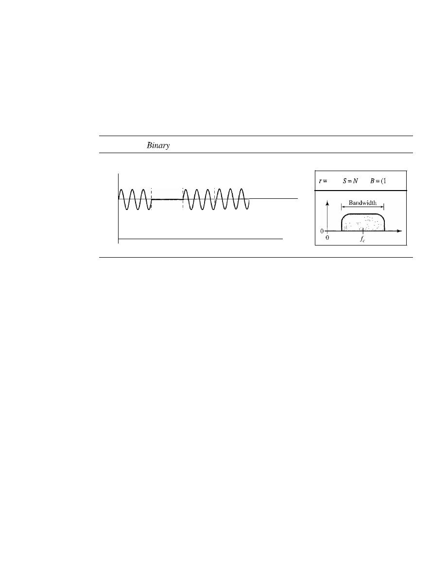
144
CHAPTER
5
ANALOG TRANSMISSION
Binary ASK (BASK)
Although we can have several levels (kinds) of signal elements, each with a different
amplitude, ASK is normally implemented using only two levels. This is referred to as
binary amplitude shift keying or
on-off keying
(OOK). The peak amplitude of one sig-
nallevel is 0; the other is the same as the amplitude of the carrier frequency. Figure 5.3
gives a conceptual view of binary ASK.
Figure 5.3
amplitude shift keying
Amplitude
Bit rate: 5
1 signal
element
o
1 signal
element
1
I signal
element
1 s
Baud rate: 5
I signal
element
o
I signal
element
I
I
Time
I
I
I
I
1
+d)S
Bandwidth for ASK
Figure 5.3 also shows the bandwidth for ASK. Although the
carrier signal is only one simple sine wave, the process of modulation produces a
nonperiodic composite signal. This signal, as was discussed in Chapter 3, has a contin-
uous set of frequencies. As we expect, the bandwidth is proportional to the signal rate
(baud rate). However, there is normally another factor involved, called
d,
which
depends on the modulation and filtering process. The value of
d
is between 0 and 1. This
means that the bandwidth can be expressed as shown, where 5 is the signal rate and the
B
is the bandwidth.
B
=(1
+d)
x
S
The formula shows that the required bandwidth has a minimum value of 5 and a
maximum value of 25. The most important point here is the location of the bandwidth.
The middle of the bandwidth is where
Ie
the carrier frequency, is located. This means if
we have a bandpass channel available, we can choose our
Ie
so that the modulated
signal occupies that bandwidth. This is in fact the most important advantage of digital-
to-analog conversion. We can shift the resulting bandwidth to match what is available.
Implementation
The complete discussion of ASK implementation is beyond the
scope of this book. However, the simple ideas behind the implementation may help us
to better understand the concept itself. Figure 5.4 shows how we can simply implement
binary ASK.
If
digital data are presented as a unipolar NRZ (see Chapter 4) digital signal with a
high voltage of
I
V and a low voltage of 0 V, the implementation can achieved by
multiplying the NRZ digital signal by the carrier signal coming from an oscillator.
When the amplitude of the NRZ signal is 1, the amplitude of the carrier frequency is
SECTION 5.1
DIGITAL-TO-ANALOG CONVERSION
145
Figure 5.4
Implementation of binary
ASK
o
Carrier signal
I
I
0
I
held; when the amplitude of the NRZ signal is 0, the amplitude of the carrier frequency
IS
zero.
Example 5.3
We have an available bandwidth of 100 kHz which spans from 200 to 300 kHz. What are the car-
rier frequency and the bit rate if we modulated our data by using ASK with
d
=
I?
Solution
The middle of the bandwidth is located at 250 kHz. This means that our carrier frequency can be
atfe
=
250 kHz. We can use the formula for bandwidth to find the bit rate (with d
=
1 and r
=
1).
B
=
(l
+
d)
x
S
=
2 x
N
=
2
X
N
=
100
kHz
......
N
=
50 kbps
r
Example 5.4
In data communications, we normally use full-duplex links with communication in both direc-
tions. We need to divide the bandwidth into two with two carrier frequencies, as shown in Fig-
ure 5.5. The figure shows the positions of two carrier frequencies and the bandwidths. The
available bandwidth for each direction is now 50 kHz, which leaves us with a data rate of 25 kbps
in each direction.
Figure 5.5
Bandwidth offull-duplex ASK used in Example 5.4
I'
B
=
50 kHz
'11
B
=
50 kHz
200
(225)
(275)
300
Multilevel ASK
The above discussion uses only two amplitude levels. We can have multilevel ASK in
which there are more than two levels. We can use 4,8, 16, or more different amplitudes
for the signal and modulate the data using 2, 3, 4, or more bits at a time. In these cases,
146
CHAPTER
5
ANALOG TRANSMISSION
r
=
2,
r
=
3,
r
=
4, and so on. Although this is not implemented with pure ASK, it is
implemented with QAM (as we will see later).
Frequency Shift Keying
In frequency shift keying, the frequency of the carrier signal is varied to represent data.
The frequency of the modulated signal is constant for the duration of one signal ele-
ment, but changes for the next signal element if the data element changes. Both peak
amplitude and phase remain constant for all signal elements.
Binary FSK (BFSK)
One way to think about binary FSK (or BFSK) is to consider two carrier frequencies. In
Figure 5.6, we have selected two carrier frequencies,f}
We use the first carrier if
the data element is 0; we use the second if the data element is 1. However, note that this
is an unrealistic example used only for demonstration purposes. Normally the carrier
frequencies are very high, and the difference between them is very small.
Figure 5.6
Binary frequency shift keying
Amplitude
Bit rate: 5
r=l
S=N
1 signal
1 signal
1 signal
1 signal
1 signal
element
element
element
element
element
Is
I'
-I
o
o
1
Baud rate: 5
As Figure 5.6 shows, the middle of one bandwidth
and the middle of the other
is
Both
and
are
apart from the midpoint between the two bands. The differ-
ence between the two frequencies is
Bandwidth for BFSK
Figure 5.6 also shows the bandwidth of FSK. Again the car-
rier signals are only simple sine waves, but the modulation creates a nonperiodic com-
posite signal with continuous frequencies. We can think of FSK as two ASK signals,
each with its own carrier frequency
Cil
or
If
the difference between the two fre-
quencies is
then the required bandwidth is
What should be the minimum value of
In Figure 5.6, we have chosen a value
greater than
(l
+
d)S.
It
can be shown that the minimum value should be at least S for
the proper operation of modulation and demodulation.
SECTION
5.1
DIGITAL-TO-ANALOG CONVERSION
147
Example 5.5
We have an available bandwidth of 100 kHz which spans from 200 to 300 kHz. What should be
the carrier frequency and the bit rate if we modulated our data by using FSK with
d
=
1
?
Solution
This problem is similar to Example 5.3, but we are modulating by using FSK. The midpoint of
the band is at 250 kHz. We choose
to be 50 kHz; this means
B
=
(1
+
d)
x S
+
=
100
2S =50
kHz
S
25 kbaud
N;;;; 25 kbps
Compared to Example 5.3, we can see the bit rate for ASK is 50 kbps while the bit rate for FSK is
25 kbps.
Implementation
There are two implementations of BFSK: noncoherent and coher-
ent. In noncoherent BFSK, there may be discontinuity in the phase when one signal
element ends and the next begins. In coherent BFSK, the phase continues through the
boundary of two signal elements. Noncoherent BFSK can be implemented by treating
BFSK as two ASK modulations and using two carrier frequencies. Coherent BFSK can
be implemented by using one
voltage-controlled oscillator
(VeO)
that changes its fre-
quency according to the input voltage. Figure 5.7 shows the simplified idea behind the
second implementation. The input to the oscillator is the unipolar NRZ signal. When
the amplitude of NRZ is zero, the oscillator keeps its regular frequency; when the
amplitude is positive, the frequency is increased.
Figure 5.7
Implementation of BFSK
1
o
1
o
veo
Voltage-controlled
oscillator
Multilevel FSK
Multilevel modulation (MFSK) is not uncommon with the FSK method. We can use
more than two frequencies. For example, we can use four different
and 14 to send 2 bits at a time. To send 3 bits at a time, we can use eight frequencies.
And so on. However, we need to remember that the frequencies need to be
apart.
For the proper operation of the modulator and demodulator, it can be shown that the
minimum value of
to be S. We can show that the bandwidth with d
=
0 is
(l
+
d)
x
S
+
(L -
B
=
Lx
S
148
CHAPTER
5
ANALOG TRANSMISSION
Example 5.6
We need to send data 3 bits at a time at a bit rate of 3 Mbps. The carrier frequency is
10 MHz. Calculate the number of levels (different frequencies), the baud rate, and the
bandwidth.
Solution
We can have
L
=
2
3
=
8. The baud rate is S
=
3 MHz/3
=
1000 Mbaud. This means that the carrier
frequencies must be 1 MHz apart
=
1 MHz). The bandwidth is
B
=
8 x 1000
=
8000. Figure 5.8
shows the allocation of frequencies and bandwidth.
Figure 5.8
Bandwidth ofMFSK used in Example 5.6
'I
13.5
MHz
I
12.5
MHz
Bandwidth
8 MHz
II
6.5
MHz
I'
I:
1
4
15
16
7.5
8.5
9.5
10.5
11.5
MHz
MHz
MHz
MHz
MHz
Phase Shift Keying
In phase shift keying, the phase of the carrier is varied to represent two or more differ-
ent signal elements. Both peak amplitude and frequency remain constant as the phase
changes. Today, PSK is more common than ASK or FSK. However, we will see
Sh0l1ly that QAM, which combines ASK and PSK, is the dominant method of digital-
to-analog modulation.
Binary PSK (BPSK)
The simplest PSK is binary PSK, in which we have only two signal elements, one with
a phase of 0°, and the other with a phase of 180°. Figure 5.9 gives a conceptual view
of PSK. Binary PSK is as simple as binary ASK with one big advantage-it is less
Figure 5.9
Binary phase shift keying
Amplitude
Bit rate: 5
o
1
I)
r=1
S=N
{I
+
d)S
I signal
I signal
I signal
I signal
I signal
element
element
element
element
element
I
Baud rate: 5
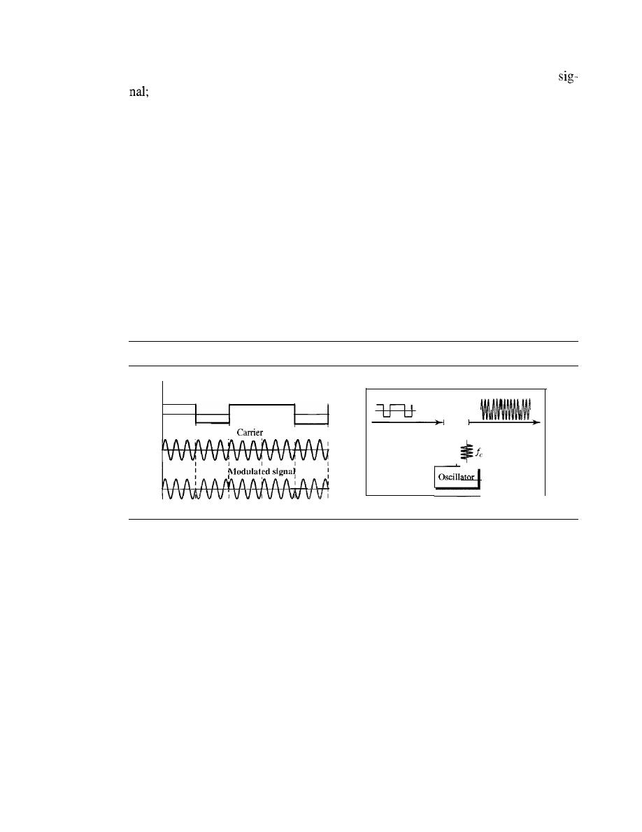
SECTION
5.1
DIGITAL-TO-ANALOG CONVERSION
149
susceptible to noise. In ASK, the criterion for bit detection is the amplitude of the
in PSK, it is the phase. Noise can change the amplitude easier than it can change
the phase. In other words, PSK is less susceptible to noise than ASK. PSK is superior to
FSK because we do not need two carrier signals.
Bandwidth
Figure 5.9 also shows the bandwidth for BPSK. The bandwidth is the
same as that for binary ASK, but less than that for BFSK. No bandwidth is wasted for
separating two carrier signals.
Implementation
The implementation of BPSK is as simple as that for ASK. The rea-
son is that the signal element with phase 180° can be seen as the complement of the sig-
nal element with phase 0°. This gives us a clue on how to implement BPSK. We use
the same idea we used for ASK but with a polar NRZ signal instead of a unipolar NRZ
signal, as shown in Figure 5.10. The polar NRZ signal is multiplied by the carrier fre-
quency; the 1 bit (positive voltage) is represented by a phase starting at 0°; the
a
bit
(negative voltage) is represented by a phase starting at 180°.
Figure 5.10
Implementation of BASK
o
1
I
I
signal
o
Multiplier
X
Quadrature PSK (QPSK)
The simplicity of BPSK enticed designers to use 2 bits at a time in each signal element,
thereby decreasing the baud rate and eventually the required bandwidth. The scheme is
called quadrature PSK or QPSK because it uses two separate BPSK modulations; one
is in-phase, the other quadrature (out-of-phase). The incoming bits are first passed
through a serial-to-parallel conversion that sends one bit to one modulator and the next
bit to the other modulator.
If
the duration of each bit in the incoming signal is
T,
the
duration of each bit sent to the corresponding BPSK signal is
2T.
This means that the
bit to each BPSK signal has one-half the frequency of the original signal. Figure 5.11
shows the idea.
The two composite signals created by each multiplier are sine waves with the
same frequency, but different phases. When they are added, the result is another sine
wave, with one of four possible phases:
45°, -45°, 135°,
and
-135°.
There are four
kinds of signal elements in the output signal
(L
=
4), so we can send 2 bits per signal
element
(r
=
2).
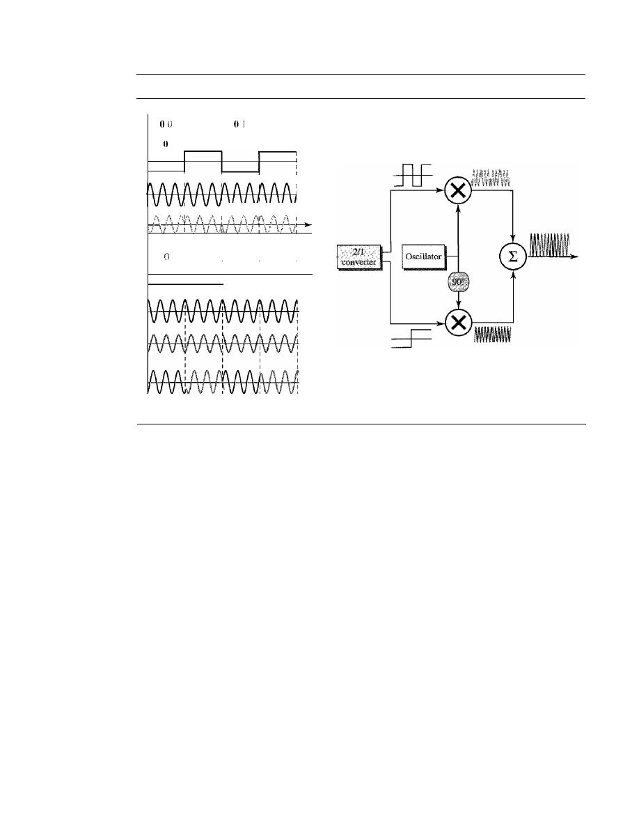
150
CHAPTER
5
ANALOG TRANSMISSION
Figure 5.11
QPSK and its implementation
1 U
1
o
1 I
1
I
I
I
I
I
I
I
I
I
I
I
I
I
I
I
I
I
I
:
0
I
I
I
I
-135
-45
135
45
Example 5.7
Find the bandwidth for a signal transmitting at 12 Mbps for QPSK. The value of
d
=
O.
Solution
For QPSK, 2 bits is carried by one signal element. This means that
r
=
2. So the signal rate (baud
rate) is S
=
N
x
(lIr)
=
6 Mbaud. With a value of
d
=
0, we have
B
=
S
=
6 MHz.
Constellation Diagram
A
constellation diagram can help us define the amplitude and phase of a signal element,
particularly when we are using two carriers (one in-phase and one quadrature), The
diagram is useful when we are dealing with multilevel ASK, PSK, or QAM (see next
section). In a constellation diagram, a signal element type is represented as a dot. The
bit or combination of bits it can carry is often written next to it.
The diagram has two axes. The horizontal X axis is related to the in-phase carrier;
the vertical
Y
axis is related to the quadrature carrier. For each point on the diagram,
four pieces of information can be deduced. The projection of the point on the X axis
defines the peak amplitude of the in-phase component; the projection of the point on
the Y axis defines the peak amplitude of the quadrature component. The length of the
line (vector) that connects the point to the origin is the peak amplitude of the signal
element (combination of the X and
Y
components); the angle the line makes with the
X axis is the phase of the signal element. All the information we need, can easily be found
on a constellation diagram. Figure 5.12 shows a constellation diagram.
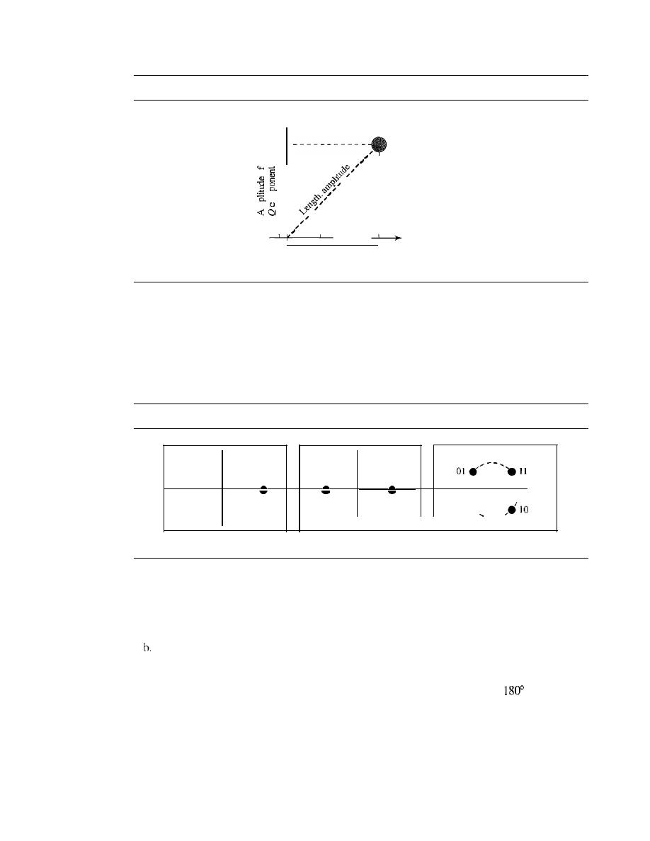
SECTION 5.1
DIGITAL-TO-ANALOG CONVERSION
151
Figure 5.12
Concept of a constellation diagram
Y
(Quadrature carrier)
I
I
o
•
I
I
I
E
.
I
0
I
E
I
I
Angle: phase
I
I
_ _
X (In-phase carrier)
Amplitude of
I
component
Example 5.8
Show the constellation diagrams for an ASK (OOK), BPSK, and QPSK signals.
Solution
Figure 5.13 shows the three constellation diagrams.
Figure 5.13
Three constellation diagrams
/
\
1
\
0
\
I
0
1
\
I
00.
a.ASK(OOK)
b.BPSK
c.QPSK
Let us analyze each case separately:
a. For ASK, we are using only an in-phase carrier. Therefore, the two points should be on the
X axis. Binary 0 has an amplitude of 0 V; binary 1 has an amplitude of 1 V (for example).
The points are located at the origin and at 1 unit.
BPSK also uses only an in-phase carrier. However, we use a polar NRZ signal for modu-
lation.
It
creates two types of signal elements, one with amplitude 1 and the other with
amplitude
-1.
This can be stated in other words: BPSK creates two different signal elements,
one with amplitude I V and in phase and the other with amplitude 1 V and
out of phase.
c. QPSK uses two carriers, one in-phase and the other quadrature. The point representing 11 is
made of two combined signal elements, both with an amplitude of 1
V.
One element is rep-
resented by an in-phase carrier, the other element by a quadrature carrier. The amplitude of
the final signal element sent for this 2-bit data element is 2112, and the phase is
45°.
The
argument is similar for the other three points. All signal elements have an amplitude of 2
112
,
but their phases are different
(45°,
135°, -135°, and -45°). Of course, we could have chosen
the amplitude of the carrier to be 1/(21/2) to make the final amplitudes 1
V.
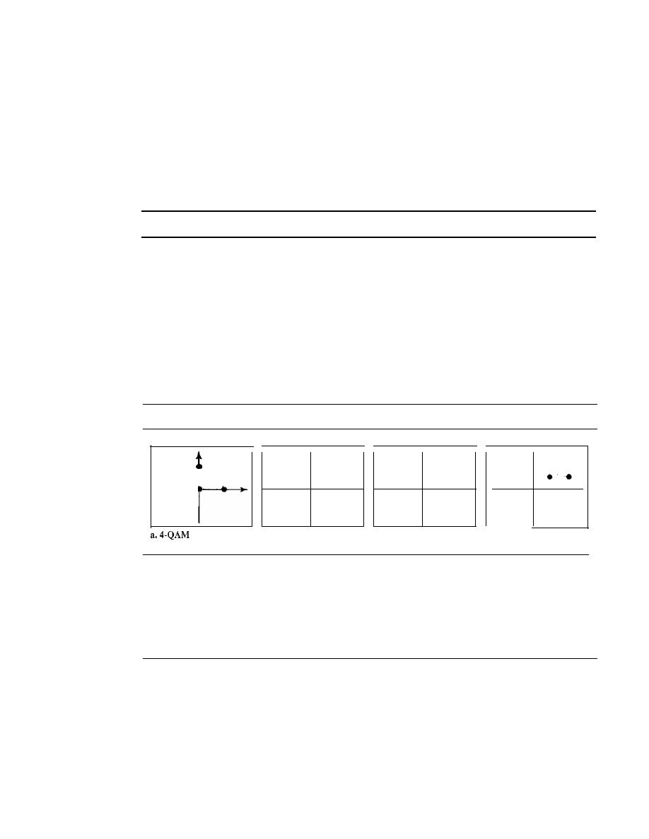
152
CHAPTER
5
ANALOG TRANSMISSION
Quadrature Amplitude Modulation
PSK is limited by the ability of the equipment to distinguish small differences in phase.
This factor limits its potential bit rate. So far, we have been altering only one of the
three characteristics of a sine wave at a time; but what if we alter two? Why not com-
bine ASK and PSK? The idea of using two carriers, one in-phase and the other quadra-
ture, with different amplitude levels for each carrier is the concept behind quadrature
amplitude modulation (QAM).
Quadrature amplitude modulation is a combination of ASK and PSK.
The possible variations of QAM are numerous. Figure 5.14 shows some of these
schemes. Figure 5.14a shows the simplest 4-QAM scheme (four different signal ele-
ment types) using a unipolar NRZ signal to modulate each carrier. This is the same
mechanism we used for ASK (OOK). Part b shows another 4-QAM using polar NRZ,
but this is exactly the same as QPSK. Part c shows another QAM-4 in which we used a
signal with two positive levels to modulate each of the two carriers. Finally, Figure 5.14d
shows a 16-QAM constellation of a signal with eight levels, four positive and four
negative.
Figure 5.14
Constellation diagrams for some QAMs
•
•
•
• •
•
•
• •
L
•
•
• •
• •
•
•
•
•
•
•
•
•
b.4-QAM
c.4.QAM
d.16·QAM
Bandwidth for QAM
The minimum bandwidth required for QAM transmission is the same as that required
for ASK and PSK transmission. QAM has the same advantages as PSK over ASK.
5.2
ANALOG-TO-ANALOG CONVERSION
Analog-to-analog conversion, or analog modulation, is the representation of analog
information by an analog signal. One may ask why we need to modulate an analog sig-
nal; it is already analog. Modulation is needed if the medium is bandpass in nature or if
only a bandpass channel is available to us. An example is radio. The government assigns
a narrow bandwidth to each radio station. The analog signal produced by each station is
a low-pass signal, all in the same range. To be able to listen to different stations, the
low-pass signals need to be shifted, each to a different range.
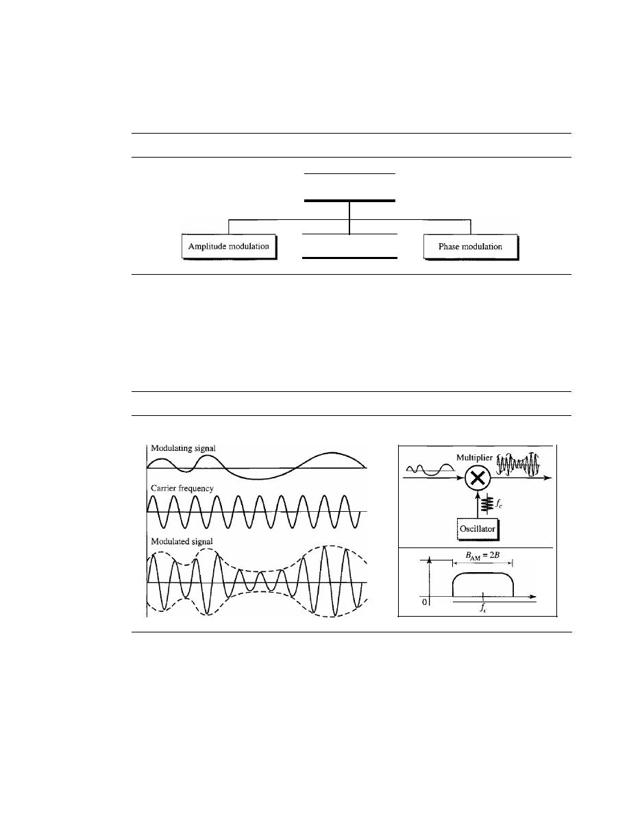
SECTION
5.2
ANALOG-TO-ANALOG CONVERSION
153
Analog-to-analog conversion
can be accomplished in three ways:
amplitude
modulation (AM), frequency modulation (FM),
and
phase modulation (PM).
FM
and PM are usually categorized together. See Figure 5.15.
Figure 5.15
Types of analog-to-analog modulation
Analog-lo-analog
conversion
Frequency modulation
Amplitude Modulation
In AM transmission, the carrier signal is modulated so that its amplitude varies with the
changing amplitudes of the modulating signal. The frequency and phase of the carrier
remain the same; only the amplitude changes to follow variations in the information. Fig-
ure 5.16 shows how this concept works. The modulating signal is the envelope of the carrier.
Figure 5.16
Amplitude modulation
o
I
As Figure 5.16 shows, AM is normally implemented by using a simple multiplier
because the amplitude of the carrier signal needs to be changed according to the ampli-
tude of the modulating signal.
AM Bandwidth
Figure 5.16 also shows the bandwidth of an AM signal. The modulation creates a band-
width that is twice the bandwidth of the modulating signal and covers a range centered
on the carrier frequency. However, the signal components above and below the carrier
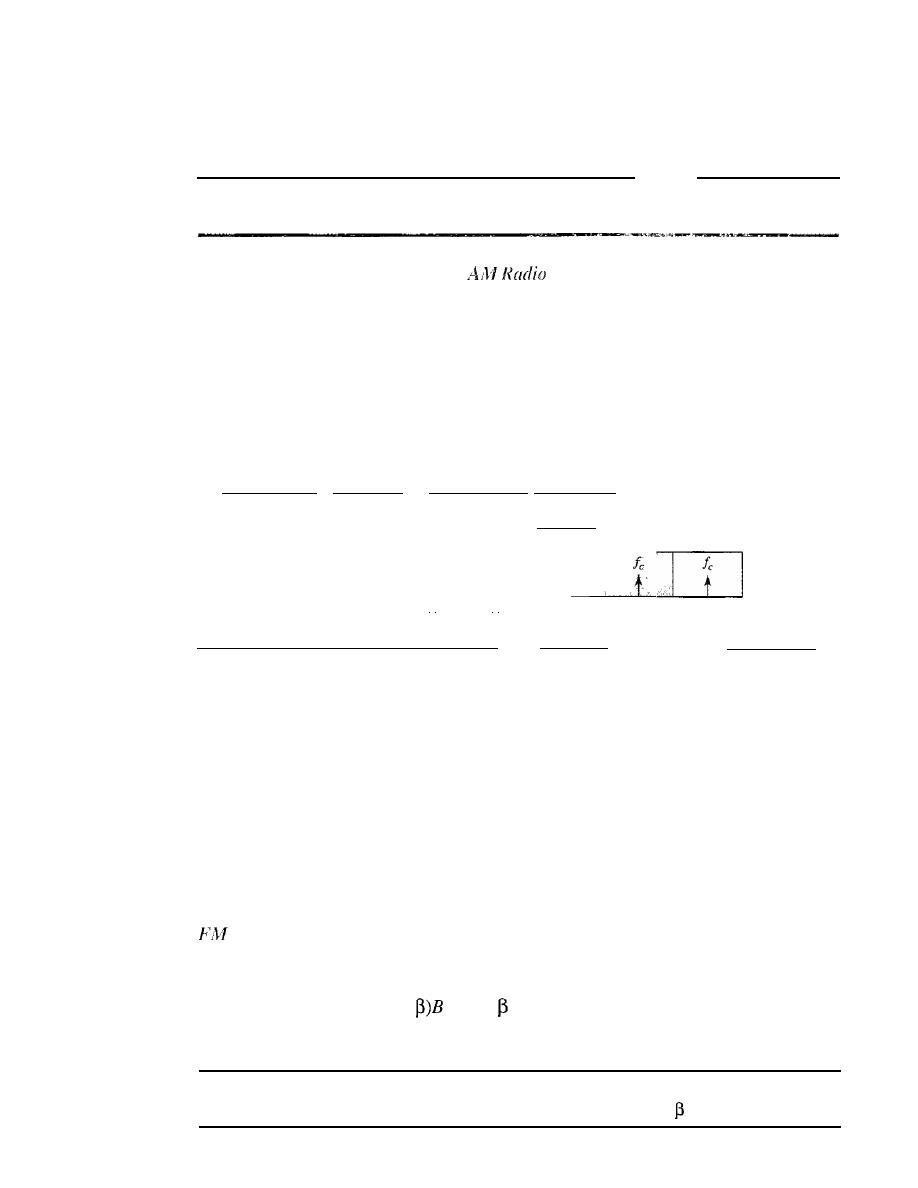
154
CHAPTER
5
ANALOG TRANSMISSION
frequency carry exactly the same information. For this reason, some implementations
discard one-half of the signals and cut the bandwidth in half.
The total bandwIdth required for AM can be determined
from the bandwidth of the audio signal:
BAM
=
2B.
Stalldard Balldwidth Allocatioll for
The bandwidth of an audio signal (speech and music) is usually 5 kHz. Therefore, an
AM radio station needs a bandwidth of 10kHz. In fact, the Federal Communications
Commission (FCC) allows 10 kHz for each AM station.
AM stations are allowed carrier frequencies anywhere between 530 and 1700 kHz
(1.7 MHz). However, each station's carrier frequency must be separated from those on
either side of it by at least 10 kHz (one AM bandwidth) to avoid interference.
If
one
station uses a carrier frequency of 1100 kHz, the next station's carrier frequency cannot
be lower than 1110 kHz (see Figure 5.17).
Figure 5.17
AM band allocation
_ _*_*_*
530
I'
, I
1700
kHz
10kHz
kHz
Frequency Modulation
In FM transmission, the frequency of the carrier signal is modulated to follow the chang-
ing voltage level (amplitude) of the modulating signal. The peak amplitude and phase of
the carrier signal remain constant, but as the amplitude of the information signal
changes, the frequency of the carrier changes correspondingly. Figure 5.18 shows the
relationships of the modulating signal, the carrier signal, and the resultant FM signal.
As Figure 5.18 shows, FM is nOimalIy implemented by using a voltage-controlled
oscillator as with FSK. The frequency of the oscillator changes according to the input
voltage which is the amplitude of the modulating signal.
Balldwidth
Figure 5.18 also shows the bandwidth of an FM signal. The actual bandwidth is diffi-
cult to determine exactly, but it can be shown empirically that it is several times that
of the analog signal or 2(1
+
where
is a factor depends on modulation technique
with a common value of 4.
The total bandwidth required for FM can be determined from
the bandwidth of the audio signal:
B
FM
=
2(1
+
)B.
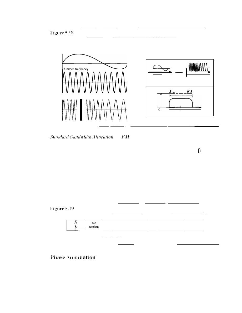
SECTION
5.2
ANALOG-TO-ANALOG CONVERSION
155
Frequency modulation
- - - - - - - - - -
Amplitude
Modulating signal (audio)
= 2(1
+
o
I
Ie
I
veo
VOltage-controlled
oscillator
Time
Time
Time
FM signal
- - - - - -
for
Radio
The bandwidth of an audio signal (speech and music) broadcast in stereo is almost
15 kHz. The FCC allows 200 kHz (0.2 MHz) for each station. This mean
=
4 with
some extra guard band. FM stations are allowed carrier frequencies anywhere between
88 and 108 MHz. Stations must be separated by at least 200 kHz to keep their band-
widths from overlapping. To create even more privacy, the FCC requires that in a given
area, only alternate bandwidth allocations may be used. The others remain unused to pre-
vent any possibility of two stations interfering with each other. Given 88 to 108 MHz as
a range, there are 100 potential PM bandwidths in an area, of which 50 can operate at
anyone time. Figure 5.19 illustrates this concept.
FM band allocation
_I
88
MHz
Ie
t
I-
200 kHz
,I
...
Ie
t
__
._--
No
station
108
MHz
In PM transmission, the phase of the carrier signal is modulated to follow the changing
voltage level (amplitude) of the modulating signal. The peak amplitude and frequency
of the carrier signal remain constant, but as the amplitude of the information signal
changes, the phase of the carrier changes correspondingly. It can proved mathemati-
cally (see Appendix C) that PM is the same as FM with one difference. In FM, the
instantaneous change in the carrier frequency is proportional to the amplitude of the
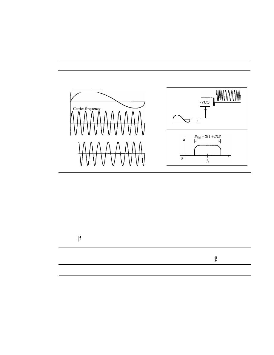
156
CHAPTER
5
ANALOG TRANSMISSION
modulating signal; in PM the instantaneous change in the carrier frequency is propor-
tional to the derivative of the amplitude of the modulating signal. Figure 5.20 shows the
relationships of the modulating signal, the carrier signal, and the resultant PM signal.
Figure 5.20
Phase modulation
Amplitude
Modulating signal (audio)
PM signal
Time
Time
Time
I
dldt
I
1
As Figure 5.20 shows, PM is normally implemented by using a voltage-controlled
oscillator along with a derivative. The frequency of the oscillator changes according to
the derivative of the input voltage which is the amplitude of the modulating signal.
PM Bandwidth
Figure 5.20 also shows the bandwidth of a PM signal. The actual bandwidth is difficult
to determine exactly, but it can be shown empirically that it is several times that of the
analog signal. Although, the formula shows the same bandwidth for FM and PM, the
value of
is lower in the case of PM (around 1 for narrowband and 3 for wideband).
The total bandwidth required for PM can be determined from the bandwidth and
maximum amplitude of the modulating signal: B
pM =
2(1
+
)B.
5.3
RECOMMENDED READING
For more details about subjects discussed in this chapter, we recommend the following
books. The items in brackets [...] refer to the reference list at the end of the text.
Books
Digital-to-analog conversion is discussed in Chapter 14 of [Pea92], Chapter 5 of
[CouOl], and Section 5.2 of [Sta04]. Analog-to-analog conversion is discussed in
Chapters 8 to 13 of [Pea92], Chapter 5 of [CouOl], and Section 5.4 of [Sta04]. [Hsu03]

SECTION
5.5
SUMMARY
157
gives a good mathematical approach to all materials discussed in this chapter. More
advanced materials can be found in [Ber96].
5.4
KEY TERMS
amplitude modulation (AM)
amplitude shift keying (ASK)
analog-to-analog conversion
carrier signal
constellation diagram
digi tal-to-analog conversion
frequency modulation (PM)
frequency shift keying (FSK)
phase modulation (PM)
phase shift keying (PSK)
quadrature amplitude modulation
(QAM)
5.5
SUMMARY
o
Digital-to-analog conversion is the process of changing one of the characteristics
of an analog signal based on the information in the digital data.
o
Digital-to-analog conversion can be accomplished in several ways: amplitude shift
keying (ASK), frequency shift keying (FSK), and phase shift keying (PSK).
Quadrature amplitude modulation (QAM) combines ASK and PSK.
o
In amplitude shift keying, the amplitude of the carrier signal is varied to create signal
elements. Both frequency and phase remain constant while the amplitude changes.
o
In frequency shift keying, the frequency of the carrier signal is varied to represent
data. The frequency of the modulated signal is constant for the duration of one sig-
nal element, but changes for the next signal element if the data element changes.
Both peak amplitude and phase remain constant for all signal elements.
o
In phase shift keying, the phase of the carrier is varied to represent two or more dif-
ferent signal elements. Both peak amplitude and frequency remain constant as the
phase changes.
o
A constellation diagram shows us the amplitude and phase of a signal element,
particularly when we are using two carriers (one in-phase and one quadrature).
o
Quadrature amplitude modulation (QAM) is a combination of ASK and PSK.
QAM uses two carriers, one in-phase and the other quadrature, with different
amplitude levels for each carrier.
o
Analog-to-analog conversion is the representation of analog information by an
analog signal. Conversion is needed if the medium is bandpass in nature or if only
a bandpass bandwidth is available to us.
o
Analog-to-analog conversion can be accomplished in three ways: amplitude modu-
lation (AM), frequency modulation (FM), and phase modulation (PM).
o
In
AM transmission, the carrier signal is modulated so that its amplitude varies with the
changing amplitudes of the modulating signal. The frequency and phase of the carrier
remain the same; only the amplitude changes to follow variations in the information.
o
In PM transmission, the frequency of the carrier signal is modulated to follow the
changing voltage level (amplitude) of the modulating signal. The peak amplitude

158
CHAPTER
5
ANALOG TRANSMISSION
and phase of the carrier signal remain constant, but as the amplitude of the infor-
mation signal changes, the frequency of the carrier changes correspondingly.
o
In PM transmission, the phase of the carrier signal is modulated to follow the
changing voltage level (amplitude) of the modulating signal. The peak amplitude
and frequency of the carrier signal remain constant, but as the amplitude of the
information signal changes, the phase of the carrier changes correspondingly.
5.6
PRACTICE SET
Review Questions
1. Define analog transmission.
2. Define carrier signal and its role in analog transmission.
3. Define digital-to-analog conversion.
4. Which characteristics of an analog signal are changed to represent the digital signal
in each of the following digital-to-analog conversion?
a.
ASK
b. FSK
c.
PSK
d.
QAM
5. Which of the four digital-to-analog conversion techniques (ASK, FSK, PSK or
QAM) is the most susceptible to noise? Defend your answer.
6.
Define constellation diagram and its role in analog transmission.
7. What are the two components of a signal when the signal is represented on a con- .
stellation diagram? Which component is shown on the horizontal axis? Which is
shown on the vertical axis?
8.
Define analog-to-analog conversion?
9.
Which characteristics of an analog signal are changed to represent the lowpass analog
signal in each of the following analog-to-analog conversions?
a.
AM
b.
FM
c.
PM
] 0. Which of the three analog-to-analog conversion techniques (AM, FM, or PM) is
the most susceptible to noise? Defend your answer.
Exercises
11.
Calculate the baud rate for the given bit rate and type of modulation.
a. 2000 bps, FSK
b. 4000 bps, ASK
c.
6000 bps, QPSK
d. 36,000 bps, 64-QAM

SECTION
5.6
PRACTICE SET
159
12. Calculate the bit rate for the given baud rate and type of modulation.
a. 1000 baud, FSK
b. 1000 baud, ASK
c. 1000 baud, BPSK
d. 1000 baud, 16-QAM
13.
What is the number of bits per baud for the following techniques?
a. ASK with four different amplitudes
b. FSK with
8
different frequencies
c.
PSK with four different phases
d. QAM with a constellation of 128 points.
14. Draw the constellation diagram for the following:
a. ASK, with peak amplitude values of 1 and 3
b. BPSK, with a peak amplitude value of 2
c. QPSK, with a peak amplitude value of
3
d. 8-QAM with two different peak amplitude values,
I
and
3,
and four different
phases.
15. Draw the constellation diagram for the following cases. Find the peak amplitude
value for each case and define the type of modulation (ASK, FSK, PSK, or QAM).
The numbers in parentheses define the values of
I
and Q respectively.
a. Two points at (2, 0) and
(3,
0).
b. Two points at (3, 0) and (-3, 0).
c. Four points at (2, 2), (-2, 2), (-2, -2), and (2, -2).
d. Two points at (0 , 2) and (0, -2).
16.
How many bits per baud can we send in each of the following cases if the signal
constellation has one of the following number of points?
a.
2
b. 4
c.
16
d. 1024
17. What is the required bandwidth for the following cases if we need to send 4000 bps?
Let
d
=
1.
a. ASK
b. FSK with
=
4 KHz
c. QPSK
d. 16-QAM
18. The telephone line has 4 KHz bandwidth. What is the maximum number of bits we
can send using each of the following techniques? Let d
=
O.
a. ASK
b. QPSK
c. 16-QAM
d.64-QAM

160
CHAPTER 5
ANALOG TRANSMISSION
19. A corporation has a medium with a I-MHz bandwidth (lowpass). The corporation
needs to create
10
separate independent channels each capable of sending at least
10
Mbps. The company has decided to use QAM technology. What is the mini-
mum number of bits per baud for each channel? What is the number of points in
the constellation diagram for each channel? Let d
=
O.
20. A cable company uses one of the cable TV channels (with a bandwidth of 6 MHz)
to provide digital communication for each resident. What is the available data rate
for each resident if the company uses a 64-QAM technique?
21.
Find the bandwidth for the following situations if we need to modulate a 5-KHz
voice.
a. AM
b.
PM
(set
=
5)
c. PM (set
=
1)
22. Find the total number of channels in the corresponding band allocated by FCC.
a. AM
b.
FM

CHAPTER 6
Bandwidth Utilization:
Multiplexing and Spreading
In real life, we have links with limited bandwidths. The wise use of these bandwidths
has been, and will be, one of the main challenges of electronic communications. How-
ever, the meaning of wise may depend on the application. Sometimes we need to combine
several low-bandwidth channels to make use of one channel with a larger bandwidth.
Sometimes we need to expand the bandwidth of a channel to achieve goals such as
privacy and antijamming. In this chapter, we explore these two broad categories of
bandwidth utilization: multiplexing and spreading. In multiplexing, our goal is effi-
ciency; we combine several channels into one. In spreading, our goals are privacy and
antijamming; we expand the bandwidth of a channel to insert redundancy, which is
necessary to achieve these goals.
Bandwidth utilization is the wise use of available bandwidth to achieve specific goals.
Efficiency can be achieved by multiplexing;
privacy and antijamming can be achieved by spreading.
6.1
MULTIPLEXING
Whenever the bandwidth of a medium linking two devices is greater than the band-
width needs of the devices, the link can be shared. Multiplexing is the set of techniques
that allows the simultaneous transmission of multiple signals across a single data link.
As data and telecommunications use increases, so does traffic. We can accommodate
this increase by continuing to add individual links each time a new channel is needed;
or we can install higher-bandwidth links and use each to carry multiple signals. As
described in Chapter 7, today's technology includes high-bandwidth media such as
optical fiber and terrestrial and satellite microwaves. Each has a bandwidth far in excess
of that needed for the average transmission signal.
If
the bandwidth of a link is greater
than the bandwidth needs of the devices connected to it, the bandwidth is wasted. An
efficient system maximizes the utilization of all resources; bandwidth is one of the
most precious resources we have in data communications.
161
162
CHAPTER
6
BANDWIDTH UTILIZATION: MULTIPLEXING AND SPREADING
In a multiplexed system,
n
lines share the bandwidth of one link. Figure 6.1 shows
the basic format of a multiplexed system. The lines on the left direct their transmission
streams to a multiplexer (MUX), which combines them into a single stream (many-to-
one). At the receiving end, that stream is fed into a demultiplexer (DEMUX), which
separates the stream back into its component transmissions (one-to-many) and
directs them to their corresponding lines. In the figure, the word link refers to the
physical path. The word channel refers to the portion of a link that carries a transmis-
sion between a given pair of lines. One link can have many
(n)
channels.
Figure
6.1
Dividing a link into channels
n
Input
lines
MUX: Multiplexer
DEMUX: Demultiplexer
D
M
E
•
U
M
·
·
X
U
·
·
X
·
I link,
11
channels
n
Output
lines
There are three basic multiplexing techniques: frequency-division multiplexing,
wavelength-division multiplexing, and time-division multiplexing. The first two are
techniques designed for analog signals, the third, for digital signals (see Figure 6.2).
Figure 6.2
Categories of multiplexing
Multiplexing
I
I
I
I
Frequency-division
I
Wavelength-division
Time-division
multiplexing
multiplexing
multiplexing
Analog
Analog
Digital
Although some textbooks consider
carrier division multiple access
(COMA) as a
fourth multiplexing category, we discuss COMA as an access method (see Chapter 12).
Frequency-Division Multiplexing
Frequency-division multiplexing (FDM) is an analog technique that can be applied
when the bandwidth of a link (in hertz) is greater than the combined bandwidths of
the signals to be transmitted. In FOM, signals generated by each sending device modu-
late different carrier frequencies. These modulated signals are then combined into a single
composite signal that can be transported
by
the link. Carrier frequencies are separated by
sufficient bandwidth to accommodate the modulated signal. These bandwidth ranges are
the channels through which the various signals travel. Channels can be separated
by
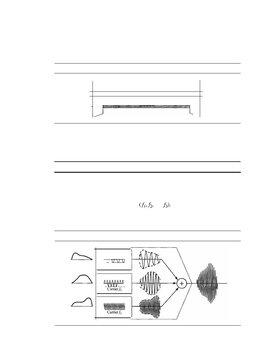
SECTION 6.1
MULTIPLEXING
163
strips of unused bandwidth-guard bands-to prevent signals from overlapping. In
addition, carrier frequencies must not interfere with the original data frequencies.
Figure 6.3 gives a conceptual view of FDM. In this illustration, the transmission path
is divided into three parts, each representing a channel that carries one transmission.
Figure 6.3
Frequency-division multiplexing
D
M
Channel
J
E
Input
U
Chanllel2
M
Output
lines
Jines
X
U
X
We consider FDM to be an analog multiplexing technique; however, this does not
mean that FDM cannot be used to combine sources sending digital signals. A digital
signal can be converted to an analog signal (with the techniques discussed in Chapter 5)
before FDM is used to multiplex them.
FDM is an analog multiplexing technique that combines analog signals.
Multiplexing Process
Figure 6.4 is a conceptual illustration of the multiplexing process. Each source gener-
ates a signal of a similar frequency range. Inside the multiplexer, these similar signals
modulates different carrier frequencies
and
The resulting modulated signals
are then combined into a single composite signal that is sent out over a media link that
has enough bandwidth to accommodate
it.
Figure 6.4
FDM process
Modulator
Modulator
V
V
V
V
Baseband
analog signals
Modulator
/\/\/\/\
V
Carrier!1
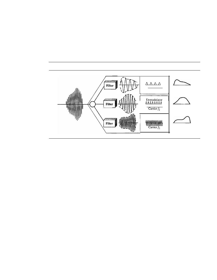
164
CHAPTER
6
BANDWIDTH UTILIZATION: MULTIPLEXING AND SPREADING
Demultiplexing Process
The demultiplexer uses a series of filters to decompose the multiplexed signal into its
constituent component signals. The individual signals are then passed to a demodulator
that separates them from their carriers and passes them to the output lines. Figure 6.5 is
a conceptual illustration of demultiplexing process.
Figure 6.5
FDM demultiplexing example
Demodulator
VVVV
Carrier!l
Baseband
analog signals
Demodulator
\
\
-
vvvvvvvv
/1'
Example 6.1
Assume that a voice channel occupies a bandwidth of 4 kHz. We need to combine three voice
channels into a link with a bandwidth of 12 kHz, from 20 to 32 kHz. Show the configuration,
using the frequency domain. Assume there are no guard bands.
Solution
We shift (modulate) each of the three voice channels to a different bandwidth, as shown in Fig-
ure 6.6. We use the 20- to 24-kHz bandwidth for the first channel, the 24- to 28-kHz bandwidth
for the second channel, and the 28- to 32-kHz bandwidth for the third one. Then we combine
them as shown in Figure 6.6. At the receiver, each channel receives the entire signal, using a
filter to separate out its own signal. The first channel uses a filter that passes frequencies
between 20 and 24 kHz and filters out (discards) any other frequencies. The second channel
uses a filter that passes frequencies between 24 and 28 kHz, and the third channel uses a filter
that passes frequencies between 28 and 32 kHz. Each channel then shifts the frequency to start
from zero.
Example 6.2
Five channels, each with a lOa-kHz bandwidth, are to be multiplexed together. What is the mini-
mum bandwidth of the link if there is a need for a guard band of 10kHz between the channels to
prevent interference?
Solution
For five channels, we need at least four guard bands. This means that the required bandwidth is at
least 5
x
100
+
4
x
10
=
540 kHz, as shown in Figure 6.7.
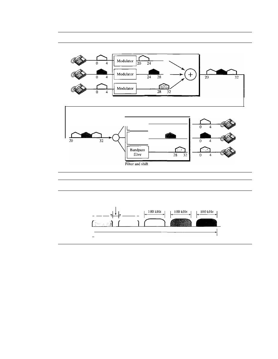
SECTION 6.1
MULTIPLEXING
165
Figure 6.6
Example 6.1
Shift and combine
Higher-bandwidth link
Bandpass
filter
Bandpass
filter
Figure 6.7
Example 6.2
Guard band
of 10 kHz
I.
100 kHz
100kHz
_I
I·
20
24
-_
_-
24
28
540 kHz
Example 6.3
Four data channels (digital), each transmitting at I Mbps, use a satellite channel of I MHz.
Design an appropriate configuration, using FDM.
Solution
The satellite channel is analog. We divide it into four channels, each channel having a 2S0-kHz
bandwidth. Each digital channel of I Mbps is modulated such that each 4 bits is modulated to
1 Hz. One solution is 16-QAM modulation. Figure 6.8 shows one possible configuration.
The Analog Carrier System
To maximize the efficiency of their infrastructure, telephone companies have tradition-
ally multiplexed signals from lower-bandwidth lines onto higher-bandwidth lines. In this
way, many switched or leased lines can be combined into fewer but bigger channels. For
analog lines, FDM is used.
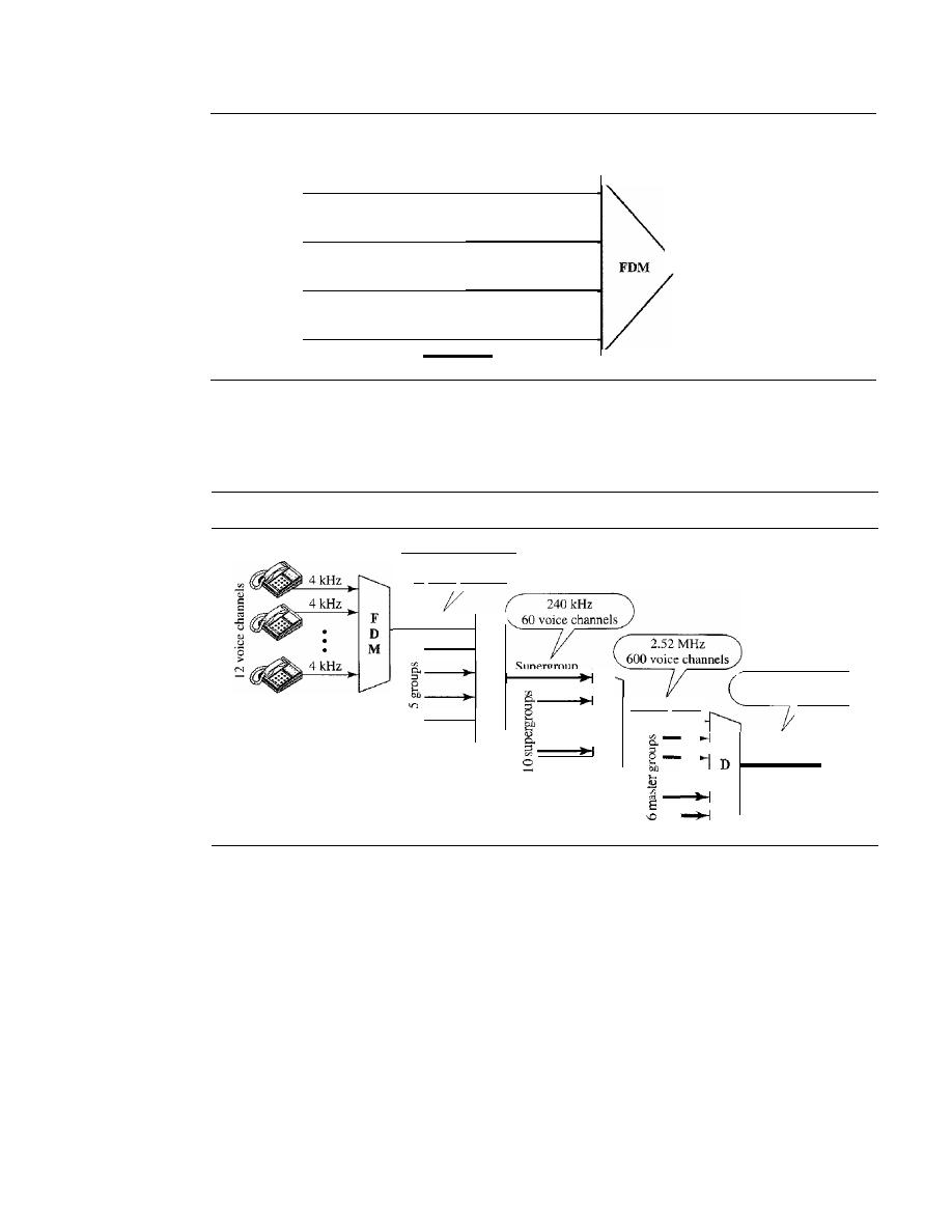
166
CHAPTER
6
BANDWIDTH UTILIZATION: MULTIPLEXING AND SPREADING
Figure 6.8
Example 6.3
I Mbps
250 kHz
Digital
Analog
I Mbps
250 kHz
Digital
Analog
I
MHz
I Mbps
250 kHz
Digital
Analog
I Mbps
250 kHz
Digital
Analog
One of these hierarchical systems used by AT&T is made up of groups, super-
groups, master groups, and jumbo groups (see Figure 6.9).
Figure 6.9
Analog hierarchy
48 kHz
12 voice channels
Jumbo
group
16.984 MHz
3600 voice channels
F
M
-
F
Master group
D
M
F
D
M
Group
In this analog hierarchy, 12 voice channels are multiplexed onto a higher-bandwidth
line to create a group. A group has 48 kHz of bandwidth and supports 12 voice channels.
At the next level, up to five groups can be multiplexed to create a composite signal
called a supergroup. A supergroup has a bandwidth of 240 kHz and supports up to
60 voice channels. Supergroups can be made up of either five groups or 60 independent
voice channels.
At the next level, 10 supergroups are multiplexed to create a master group. A
master group must have 2.40 MHz of bandwidth, but the need for guard bands between
the supergroups increases the necessary bandwidth to 2.52 MHz. Master groups support
up to 600 voice channels.
Finally, six master groups can be combined into a jumbo group. A jumbo group
must have 15.12 MHz (6 x 2.52 MHz) but is augmented to 16.984 MHz to allow for
guard bands between the master groups.

SECTION
6.1
MULTIPLEXING
167
Other Applications of FDM
A very common application of FDM is AM and FM radio broadcasting. Radio uses the
air as the transmission medium. A special band from 530 to 1700 kHz is assigned to AM
radio. All radio stations need to share this band. As discussed in Chapter 5, each AM sta-
tion needs 10kHz of bandwidth. Each station uses a different carrier frequency, which
means it is shifting its signal and multiplexing. The signal that goes to the air is a combi-
nation of signals. A receiver receives all these signals, but filters (by tuning) only the one
which is desired. Without multiplexing, only one AM station could broadcast to the com-
mon link, the air. However, we need to know that there is physical multiplexer or demulti-
plexer here. As we will see in Chapter 12 multiplexing is done at the data link layer.
The situation is similar in FM broadcasting. However, FM has a wider band of 88
to 108 MHz because each station needs a bandwidth of 200 kHz.
Another common use of FDM is in television broadcasting. Each TV channel has
its own bandwidth of 6 MHz.
The first generation of cellular telephones (still in operation) also uses FDM. Each
user is assigned two 30-kHz channels, one for sending voice and the other for receiving.
The voice signal, which has a bandwidth of 3 kHz (from 300 to 3300 Hz), is modulated by
using FM. Remember that an FM signal has a bandwidth 10 times that of the modulating
signal, which means each channel has 30 kHz (10 x 3) of bandwidth. Therefore, each user
is given, by the base station, a 60-kHz bandwidth
in
a range available at the time of the call.
Example 6.4
The Advanced Mobile Phone System (AMPS) uses two bands. The first band of 824 to 849 MHz
is used for sending, and 869 to 894 MHz is used for receiving. Each user has a bandwidth of
30 kHz in each direction. The 3-kHz voice is modulated using FM, creating 30 kHz of modulated
signal. How many people can use their cellular phones simultaneously?
Solution
Each band is 25 MHz.
If
we divide 25 MHz by 30 kHz, we get 833.33.
In
reality, the band is divided
into 832 channels. Of these, 42 channels are used for control, which means only 790 channels are
available for cellular phone users. We discuss AMPS in greater detail in Chapter 16.
Implementation
FDM can be implemented very easily. In many cases, such as radio and television
broadcasting, there is no need for a physical multiplexer or demultiplexer. As long as
the stations agree to send their broadcasts to the air using different carrier frequencies,
multiplexing is achieved. In other cases, such as the cellular telephone system, a base
station needs to assign a carrier frequency to the telephone user. There is not enough
bandwidth in a cell to permanently assign a bandwidth range to every telephone user.
When a user hangs up, her or his bandwidth is assigned to another caller.
Wavelength-Division Multiplexing
Wavelength-division multiplexing (WDM) is designed to use the high-data-rate
capability of fiber-optic cable. The optical fiber data rate is higher than the data rate of
metallic transmission cable. Using a fiber-optic cable for one single line wastes the
available bandwidth. Multiplexing allows us to combine several lines into one.
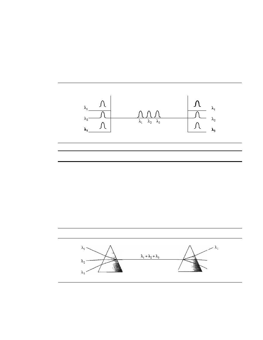
168
CHAPTER
6
BANDWIDTH UTILIZATION: MULTIPLEXING AND SPREADING
WDM is conceptually the same as FDM, except that the multiplexing and demulti-
plexing involve optical signals transmitted through fiber-optic channels. The idea is the
same: We are combining different signals of different frequencies. The difference is
that the frequencies are very high.
Figure 6.10 gives a conceptual view of a WDM multiplexer and demultiplexer.
Very narrow bands of light from different sources are combined to make a wider band
of light. At the receiver, the signals are separated by the demultiplexer.
Figure 6.10
Wavelength-division multiplexing
+
+
WDM
is
an
analog multiplexing technique to combine optical signals.
Although WDM technology is very complex, the basic idea is very simple. We
want to combine multiple light sources into one single light at the multiplexer and do
the reverse at the demultiplexer. The combining and splitting of light sources are easily
handled by a prism. Recall from basic physics that a prism bends a beam of light based
on the angle of incidence and the frequency. Using this technique, a multiplexer can be
made to combine several input beams of light, each containing a narrow band of fre-
quencies, into one output beam of a wider band of frequencies. A demultiplexer can
also be made to reverse the process. Figure 6.11 shows the concept.
:Figure 6.11
Prisms in wavelength-division multiplexing and demultiplexing
Multiplexer
Fiber-optic cable
Demultiplexer
One application of WDM is the SONET network in which multiple optical
fiber lines are multiplexed and demultiplexed. We discuss SONET in Chapter 17.
A new method, called dense WDM (DWDM), can multiplex a very large number
of channels by spacing channels very close to one another. It achieves even greater
efficiency.
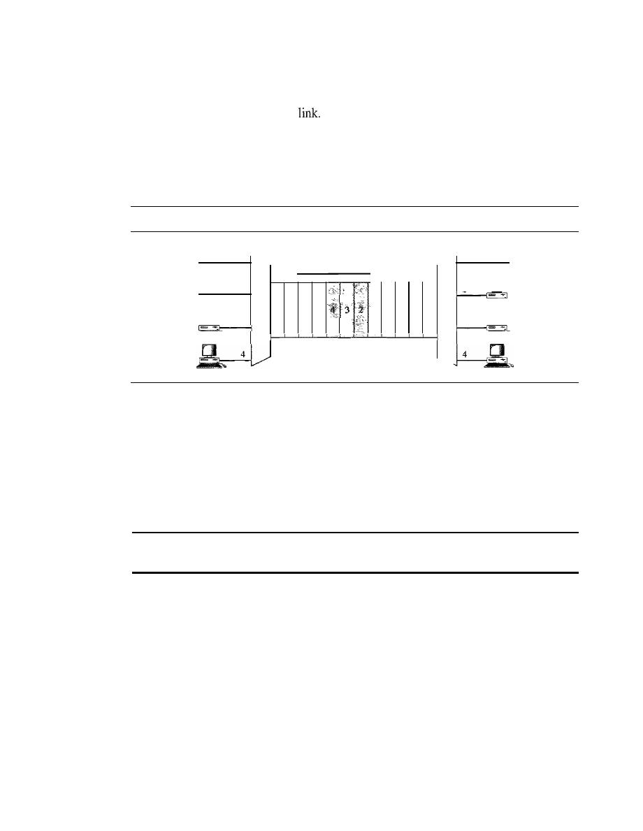
SECTION
6.1
MULTIPLEXING
169
Synchronous Time-Division Multiplexing
Time-division multiplexing (TDM) is a digital process that allows several connections
to share the high bandwidth of a
Instead of sharing a portion of the bandwidth as in
FDM, time is shared. Each connection occupies a portion of time in the link. Figure 6.12
gives a conceptual view of TDM. Note that the same link is used as in FDM; here, how-
ever, the link is shown sectioned by time rather than by frequency. In the figure, portions
of signals 1,2,3, and 4 occupy the link sequentially.
Figure 6.12
TDM
Data flow
.
D
2
E
l ' 4 3 2 1 M
U
3
X
2
M
U
4
3
2
1
3
X
Note that in Figure 6.12 we are concerned with only multiplexing, not switching.
This means that all the data in a message from source 1 always go to one specific desti-
nation, be it 1, 2, 3, or 4. The delivery is fixed and unvarying, unlike switching.
We also need to remember that TDM is, in principle, a digital multiplexing technique.
Digital data from different sources are combined into one timeshared link. However, this
does not mean that the sources cannot produce analog data; analog data can be sampled,
changed to digital data, and then multiplexed by using TDM.
TDM is a digital multiplexing technique for combining
several low-rate channels into one high-rate one.
We can divide TDM into two different schemes: synchronous and statistical. We first
discuss synchronous TDM and then show how statistical TDM differs. In synchronous
TDM, each input connection has an allotment in the output even if it is not sending data.
Time Slots and Frames
In synchronous TDM, the data flow of each input connection is divided into units, where
each input occupies one input time slot. A unit can be 1 bit, one character, or one block of
data. Each input unit becomes one output unit and occupies one output time slot. How-
ever, the duration of an output time slot is
n
times shorter than the duration of an input
time slot.
If
an input time slot is
T
s, the output time slot is
Tin
s, where
n
is the number
of connections. In other words, a unit in the output connection has a shorter duration; it
travels faster. Figure 6.13 shows an example of synchronous TDM where
n
is 3.
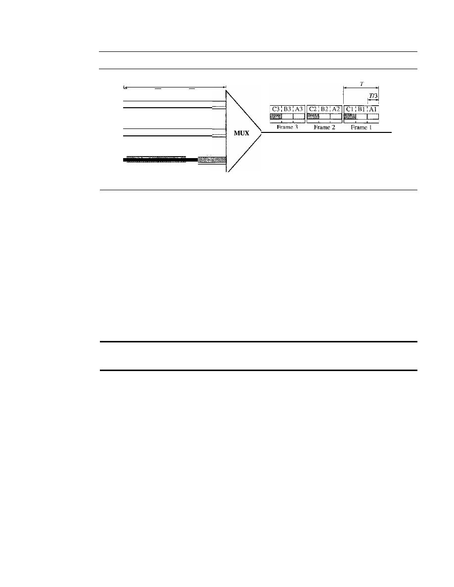
170
CHAPTER
6
BANDWIDTH UTILIZATION: MULTIPLEXING AND SPREADING
Figure 6.13
Synchronous time-division multiplexing
Data are taken from each
line every T s.
Each frame is 3 time slots.
Each time slot duration is
Tf3
s.
Bl
T
Al
Cl
J i l
A2
B2
T
C2
J l f
T
C3
A3
B3
In synchronous TDM, a round of data units from each input connection is collected
into a frame (we will see the reason for this shortly).
If
we have n connections, a frame
is divided into
n
time slots and one slot is allocated for each unit, one for each input
line.
If
the duration of the input unit is T, the duration of each slot is Tin and the dura-
tion of each frame is
T
(unless a frame carries some other information, as we will see
shortly).
The data rate of the output link must be n times the data rate of a connection to
guarantee the flow of data. In Figure 6.13, the data rate of the link is 3 times the data
rate of a connection; likewise, the duration of a unit on a connection is 3 times that of
the time slot (duration of a unit on the link). In the figure we represent the data prior to
multiplexing as 3 times the size of the data after multiplexing. This is just to convey the
idea that each unit is 3 times longer in duration before multiplexing than after.
In synchronous TDM, the data rate of the link is
n
times faster,
and the unit duration is
n times shorter.
Time slots are grouped into frames. A frame consists of one complete cycle of
time slots, with one slot dedicated to each sending device. In a system with
n
input
lines, each frame has n slots, with each slot allocated to carrying data from a specific
input line.
Example 6.5
In Figure 6.13, the data rate for each input connection is 3 kbps. If 1 bit at a time is multiplexed (a
unit is 1 bit), what is the duration of (a) each input slot, (b) each output slot, and (c) each frame?
Solution
We can answer the questions as follows:
a. The data rate of each input connection is 1 kbps. This means that the bit duration is 111000 s
or 1 ms. The duration of the input time slot is 1 ms (same as bit duration).
b. The duration of each output time slot is one-third of the input time slot. This means that the
duration of the output time slot is 1/3 ms.
c. Each frame carries three output time slots. So the duration of a frame is 3 x 113 ms, or 1 ms.
The duration of a frame is the same as the duration of an input unit.
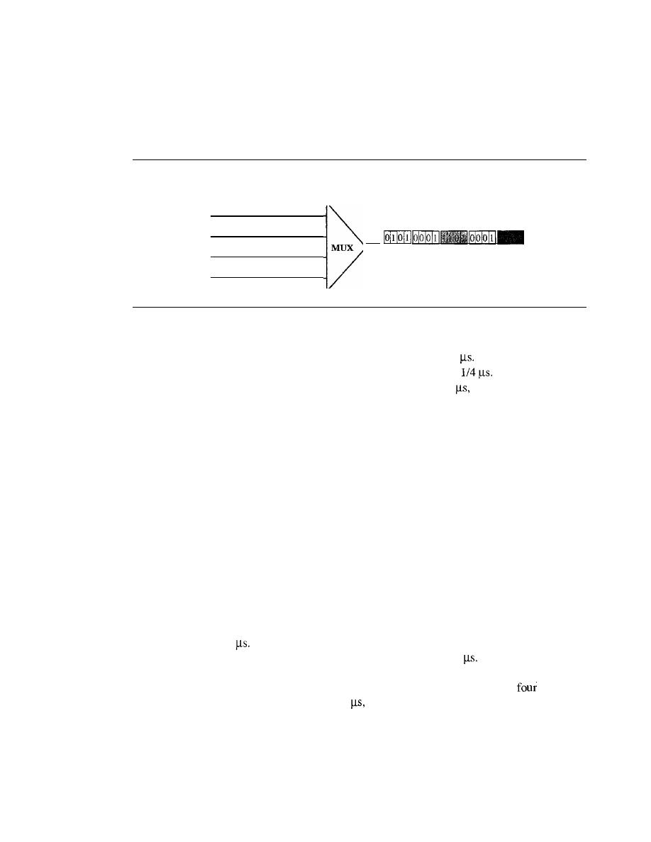
SECTION
6.1
MULTIPLEXING
171
Example 6.6
Figure 6.14 shows synchronous TOM with a data stream for each input and one data stream for
the output. The unit of data is 1 bit. Find (a) the input bit duration, (b) the output bit duration,
(c) the output bit rate, and (d) the output frame rate.
Figure 6.14
Example 6.6
I Mbps
• •• 1
1 Mbps
• •• 0
0
0
0
1 Mbps
• •• 1
0
0
1 Mbps
• •• 0
0
0
o
o
Frames
•••
Solution
We can answer the questions as follows:
a. The input bit duration is the inverse of the bit rate: 1/1 Mbps
=
1
b. The output bit duration is one-fourth of the input bit duration, or
c. The output bit rate is the inverse of the output bit duration or 1/4
or 4 Mbps. This can also
be deduced from the fact that the output rate is 4 times as fast as any input rate; so the output
rate
=
4 x 1 Mbps
=
4 Mbps.
d. The frame rate is always the same as any input rate. So the frame rate is 1,000,000 frames per
second. Because we are sending 4 bits in each frame, we can verify the result of the previous
question by multiplying the frame rate by the number of bits per frame.
Example 6.7
Four l-kbps connections are multiplexed together. A unit is I bit. Find (a) the duration of I bit
before multiplexing, (b) the transmission rate of the link, (c) the duration of a time slot, and
(d) the duration of a frame.
Solution
We can answer the questions as follows:
a. The duration of 1 bit before multiplexing is 1/1 kbps, or 0.001 s
(l
ms).
b.
The rate of the link is 4 times the rate of a connection, or 4 kbps.
c. The duration of each time slot is one-fourth of the duration of each bit before multiplexing,
or 1/4 ms or 250
Note that we can also calculate this from the data rate of the link, 4 kbps.
The bit duration is the inverse of the data rate, or 1/4 kbps or 250
d. The duration of a frame is always the same as the duration of a unit before multiplexing, or
I ms. We can also calculate this in another way. Each frame in this case has
time slots.
So the duration of a frame is 4 times 250
or I ms.
Interleaving
TDM can be visualized as two fast-rotating switches, one on the multiplexing side and
the other on the demultiplexing side. The switches are synchronized and rotate at the
same speed, but in opposite directions. On the multiplexing side, as the switch opens
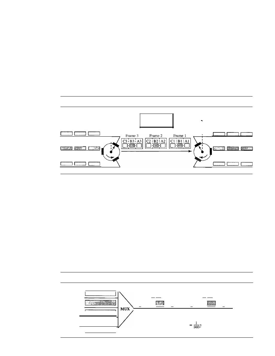
172
CHAPTER
6
BANDWIDTH UTILIZATION: MULTIPLEXING AND SPREADING
in front of a connection, that connection has the opportunity to send a unit onto the
path. This process is called
interleaving.
On the demultiplexing side, as the switch
opens in front of a connection, that connection has the opportunity to receive a unit
from the path.
Figure 6.15 shows the interleaving process for the connection shown in Figure 6.13.
In this figure, we assume that no switching is involved and that the data from the first
connection at the multiplexer site go to the first connection at the demultiplexer. We
discuss switching in Chapter 8.
Figure 6.15
Interleaving
A3
A2
Al
B3
B2
Bl
C3
C2
CI
r - - - - - - - - - -
Synchronization
- - - - - - - - -
I
I
I
I
I
A3
A2
Al
B3
B2
Bl
C3
C2
Cl
Example 6.8
Four channels are multiplexed using TDM.
If
each channel sends 100 bytesis and we multiplex
1 byte per channel, show the frame traveling on the
link,
the size of the frame, the duration of a
frame, the frame rate, and the bit rate for the link.
Solution
The multiplexer is shown in Figure 6.16. Each frame carries 1 byte from each channel; the size of
each frame, therefore, is 4 bytes, or 32 bits. Because each channel is sending 100 bytes/s and a
frame carries 1 byte from each channel, the frame rate must be 100 frames per second. The dura-
tion of a frame is therefore 11100 s. The link is carrying 100 frames per second, and since each
frame contains 32 bits, the bit rate is 100 x 32, or 3200 bps. This is actually 4 times the bit rate of
each channel, which is 100 x 8
=
800 bps.
Figure 6.16
Example 6.8
-
100
bytes/s
Frame 4 bytes
Frame 4 bytes
32 bits
32 bits
II
'I ...
II
II
100 frames/s
3200 bps
Frame duration
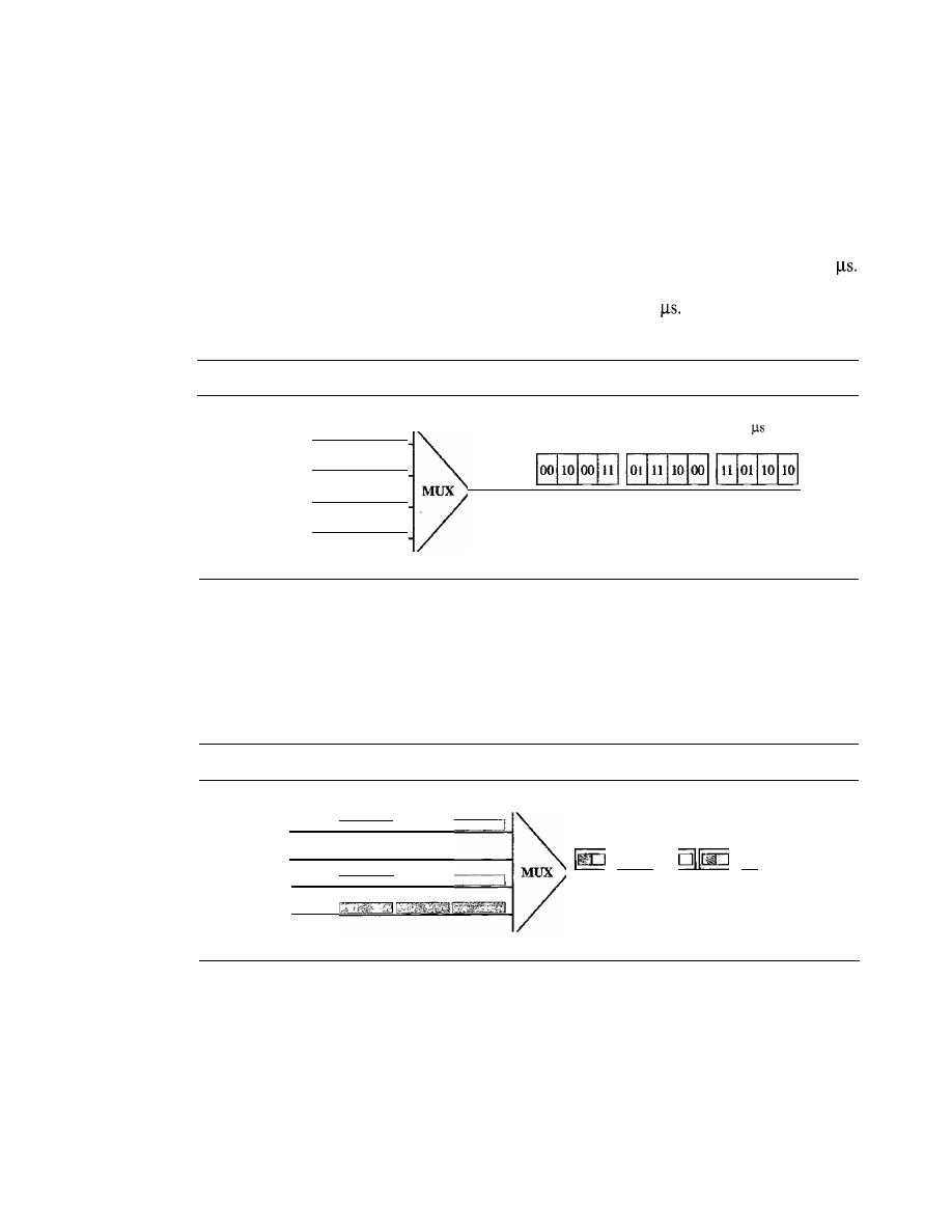
SECTION 6.1
MULTIPLEXING
173
Example 6.9
A multiplexer combines four 100-kbps channels using a time slot of 2 bits. Show the output with
four arbitrary inputs. What is the frame rate? What is the frame duration? What is the bit rate?
What is the bit duration?
Solution
Figure 6.17 shows the output for four arbitrary inputs. The link carries 50,000 frames per second
since each frame contains 2 bits per channel. The frame duration is therefore 1/50,000 s or 20
The frame rate is 50,000 frames per second, and each frame carries 8 bits; the bit rate is 50,000
x
8
=
400,000 bits or 400 kbps. The bit duration is 1/400,000 s, or 2.5
Note that the frame dura-
tion is 8 times the bit duration because each frame is carrying 8 bits.
Figure 6.17
Example 6.9
·
..
110010
100 kbps
...
001010
100 kbps
·
..
101 101
100 kbps
·
..
000111
100 kbps
Frame duration
=
lI50,000 s
=
20
Frame: 8 bits
Frame: 8 bits
Frame: 8 bits
...
50,000 frames/s
400kbps
Empty Slots
Synchronous TDM is not as efficient as it could be. If a source does not have data to
send, the corresponding slot in the output frame is empty. Figure 6.18 shows a case in
which one of the input lines has no data to send and one slot in another input line has
discontinuous data.
Figure 6.18
Empty slots
II
II
0110
01
The first output frame has three slots filled, the second frame has two slots filled,
and the third frame has three slots filled. No frame is full. We learn in the next section
that statistical TDM can improve the efficiency by removing the empty slots from the
frame.
Data Rate Management
One problem with TDM is how to handle a disparity in the input data rates. In all our
discussion so far, we assumed that the data rates of all input lines were the same. However,
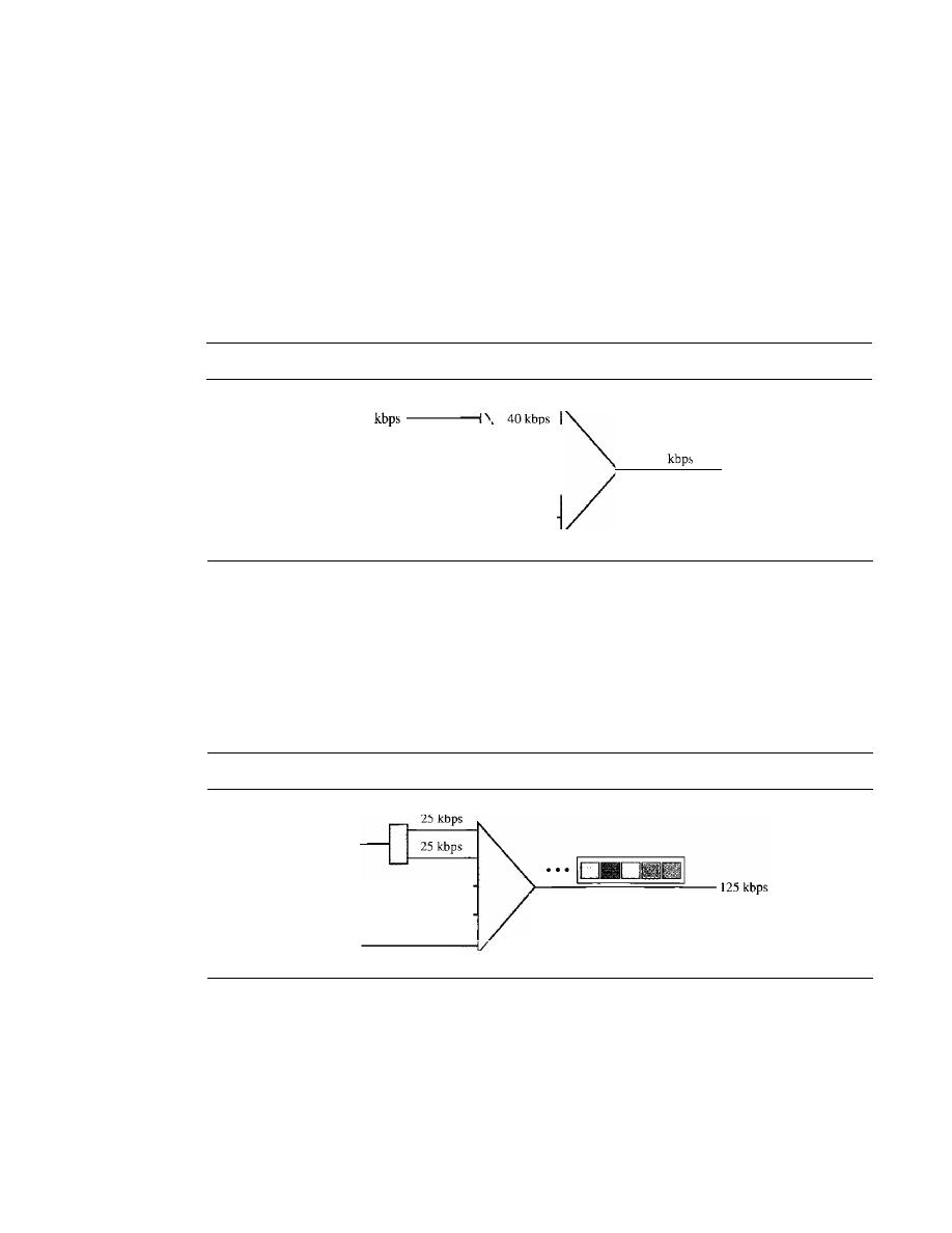
174
CHAPTER
6
BANDWIDTH UTILIZATION: MULTIPLEXING AND SPREADING
if data rates are not the same, three strategies, or a combination of them, can be used.
We call these three strategies multilevel multiplexing, multiple-slot allocation, and
pulse stuffing.
Multilevel Multiplexing
Multilevel multiplexing is a technique used when the data
rate of an input line is a multiple of others. For example, in Figure 6.19, we have two
inputs of 20 kbps and three inputs of 40 kbps. The first two input lines can be multi-
plexed together to provide a data rate equal to the last three. A second level of multi-
plexing can create an output of 160 kbps.
Figure 6.19
Multilevel multiplexing
20
>------t
20 kbps
- - - - I
40
kbps
- - - - - - - - 1
40 kbps
- - - - - - - - 1
40
kbps
- - - - - - - - 1
160
Multiple-Slot Allocation
Sometimes it is more efficient to allot more than one slot in
a frame to a single input line. For example, we might have an input line that has a data
rate that is a multiple of another input. In Figure 6.20, the input line with a SO-kbps data
rate can be given two slots in the output. We insert a serial-to-parallel converter in the
line to make two inputs out of one.
Figure 6.20
Multiple-slot multiplexing
50 kbps
25 kbps
- - - - - - - 1
25 kbps
- - - - - - - 1
25 kbps
The
input with
a
50-kHz data rate has two
slots in each frame.
Pulse Stuffing
Sometimes the bit rates of sources are not multiple integers of each
other. Therefore, neither of the above two techniques can be applied. One solution is to
make the highest input data rate the dominant data rate and then add dummy bits to the
input lines with lower rates. This will increase their rates. This technique is called pulse
stuffing, bit padding, or bit stuffing. The idea is shown in Figure 6.21. The input with a
data rate of 46 is pulse-stuffed to increase the rate to 50 kbps. Now multiplexing can
take place.
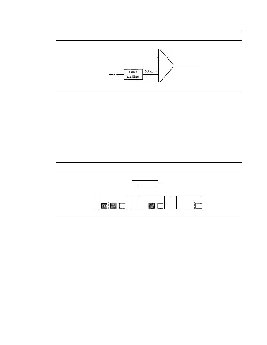
SECTION 6.1
MULTIPLEXING
175
Figure 6.21
Pulse stuffing
50
kbps - - - - - - - - - - 1
50
kbps - - - - - - - - - - 1
46kbps
150
kbps
Frame Synchronizing
The implementation of TDM is not as simple as that of FDM. Synchronization between
the multiplexer and demultiplexer is a major issue. If the. multiplexer and the demulti-
plexer are not synchronized, a bit belonging to one channel may be received by the
wrong channel. For this reason, one or more synchronization bits are usually added
to
the beginning of each frame. These bits, called framing bits, follow a pattern, frame to
frame, that allows the demultiplexer to synchronize with the incoming stream so that it
can separate the time slots accurately. In most cases, this synchronization information
consists of
1
bit per frame, alternating between 0 and I, as shown in Figure 6.22.
Figure 6.22
Framing bits
I
1
0
1
I
Synchronization
pattern
Frame 3
Frame 2
Frame 1
C3
I
B3
I
A3
182
I
A2
CI
I
I
Al
0
I
I
I
I
I
Example 6.10
We have four sources, each creating 250 characters per second. If the interleaved unit is a character
and 1 synchronizing bit is added to each frame, find (a) the data rate of each source, (b) the duration
of each character in each source, (c) the frame rate, (d) the duration of each frame, (e) the number of
bits in each frame, and
(f)
the data rate of the link.
Solution
We can answer the questions as follows:
a. The data rate of each source is 250
x
8
=
2000 bps
=
2 kbps.
b. Each source sends 250 characters per second; therefore, the duration of a character is 1/250 s,
or4 ms.
c. Each frame has one character from each source, which means the link needs to send
250 frames per second to keep the transmission rate of each source.
d. The duration of each frame is
11250
s, or 4 ms. Note that the duration of each frame is the
same as the duration of each character coming from each source.
e. Each frame carries 4 characters and I extra synchronizing bit. This means that each frame is
4 x 8
+
1
=
33 bits.
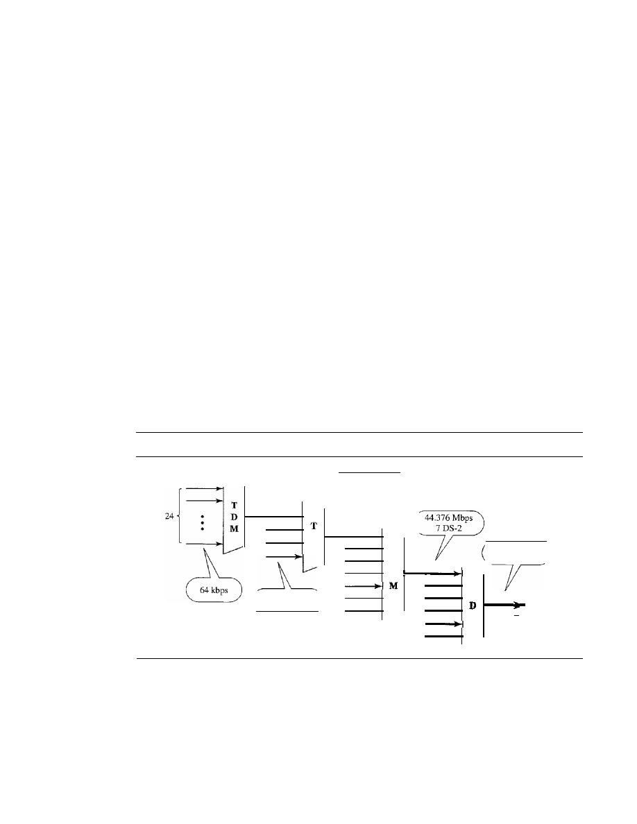
176
CHAPTER
6
BANDWIDTH UTILIZATION: MULTIPLEXING AND SPREADING
f.
The link sends 250 frames per second, and each frame contains 33 bits. This means that the
data rate of the link is 250 x 33, or 8250 bps. Note that the bit rate of the link is greater than
the combined bit rates of the four channels. If we add the bit rates of four channels, we get
8000 bps. Because 250 frames are traveling per second and each contains 1 extra bit for
synchronizing, we need to add 250 to the sum to get 8250 bps.
Example 6.11
Two channels, one with a bit rate of 100 kbps and another with a bit rate of 200 kbps, are to be
multiplexed. How this can be achieved? What is the frame rate? What is the frame duration?
What is the bit rate of the link?
Solution
We can allocate one slot to the first channel and two slots to the second channel. Each frame car-
ries 3 bits. The frame rate is 100,000 frames per second because it carries 1 bit from the first
channel. The frame duration is 1/100,000 s, or 10 ms. The bit rate is 100,000 frames/s x 3 bits per
frame, or 300 kbps. Note that because each frame carries 1 bit from the first channel, the bit rate
for the first channel is preserved. The bit rate for the second channel is also preserved because
each frame carries 2 bits from the second channel.
Digital Signal Service
Telephone companies implement TDM through a hierarchy of digital signals, called
digital signal (DS) service or digital hierarchy. Figure 6.23 shows the data rates sup-
ported by each level.
Figure 6.23
Digital hierarchy
OS-4
274.176 Mbps
60S-3
OS-3
T
M
6.312 Mbps
405-1
T
D
OS-2
D
M
1.544 Mbps
24 DS-O
OS-1
os-o
o
A DS-O service is a single digital channel of 64 kbps.
ODS-I is a 1.544-Mbps service; 1.544 Mbps is 24 times 64 kbps plus 8 kbps of
overhead. It can be used as a single service for 1.544-Mbps transmissions, or it can
be used to multiplex 24 DS-O channels or to carry any other combination desired
by the user that can fit within its 1.544-Mbps capacity.
o
DS-2 is a 6.312-Mbps service; 6.312 Mbps is 96 times 64 kbps plus 168 kbps of
overhead.
It
can be used as a single service for 6.312-Mbps transmissions; or it can

SECTION
6.1
MULTIPLEXING
177
be used to multiplex 4 DS-l channels, 96 DS-O channels, or a combination of these
service types.
o
DS-3
is a 44.376-Mbps service; 44.376 Mbps is 672 times 64 kbps plus 1.368 Mbps
of overhead.
It
can be used as a single service for 44.376-Mbps transmissions; or it
can be used to multiplex 7 DS-2 channels, 28 DS-l channels, 672 DS-O channels,
or a combination of these service types.
o
DS-4
is a 274. 176-Mbps service; 274.176 is 4032 times 64 kbps plus 16.128 Mbps of
overhead.
It
can be used to multiplex 6 DS-3 channels, 42 DS-2 channels, 168 DS-l
channels, 4032 DS-O channels, or a combination of these service types.
T Lines
DS-O, DS-l, and so on are the names of services. To implement those services, the tele-
phone companies use
T
lines
(T-l to T-4). These are lines with capacities precisely
matched to the data rates of the DS-l to DS-4 services (see Table 6.1). So far only T-l
and T-3 lines are commercially available.
Table 6.1
DS and T line rates
Sen/ice
Line
Rate (Mbps)
Voice Channels
DS-1
T-1
1.544
24
DS-2
T-2
6.312
96
DS-3
T-3
44.736
672
DS-4
T-4
274.176
4032
The T-l line is used to implement DS-l; T-2 is used to implement DS-2; and so on.
As you can see from Table 6.1, DS-O is not actually offered as a service, but it has been
defined as a basis for reference purposes.
T Lines for Analog Transmission
T lines are digital lines designed for the transmission of digital data, audio, or video.
However, they also can be used for analog transmission (regular telephone connec-
tions), provided the analog signals are first sampled, then time-division multiplexed.
The possibility of using T lines as analog carriers opened up a new generation of
services for the telephone companies. Earlier, when an organization wanted 24 separate
telephone lines, it needed to run 24 twisted-pair cables from the company to the central
exchange. (Remember those old movies showing a busy executive with 10 telephones
lined up on his desk? Or the old office telephones with a big fat cable running from
them? Those cables contained a bundle of separate lines.) Today, that same organization
can combine the 24 lines into one T-l line and run only the T-l line to the exchange.
Figure 6.24 shows how 24 voice channels can be multiplexed onto one T-I line. (Refer
to Chapter 5 for PCM encoding.)
The
T-1
Frame
As noted above, DS-l requires 8 kbps of overhead. To understand how
this overhead is calculated, we must examine the format of a 24-voice-channel frame.
The frame used on a T-l line is usually 193 bits divided into 24 slots of 8 bits each
plus 1 extra bit for synchronization (24 x 8
+
1
=
193); see Figure 6.25. In other words,
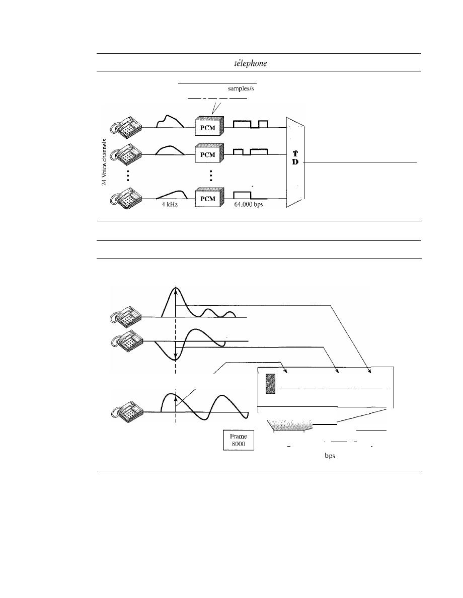
178
CHAPTER
6
BANDWIDTH UTILIZATION: MULTIPLEXING AND SPREADING
Figure 6.24
T-l
line for multiplexing
lines
Sampling at 8000
Llsing 8 bits per sample
M
T-I line 1.544 Mbps
24 x 64 kbps
+
8 kbps overhead
Figure 6.25
T-l
frame structure
Samplen
I
1 frame= 193 bits
Channel
I··
·1
Channel
II
Channel
I
24
2
I
1 bit
8 bits
8 bits
8 bits
Frame
I
Frame
II
Frame
.
.
.
...
n
2
1
T- I: 8000 frames/s = 8000 x 193
= 1.544 Mbps
each slot contains one signal segment from each channel; 24 segments are interleaved
in one frame.
If
a T-l line carries 8000 frames, the data rate is 1.544 Mbps (193 x 8000
=
1.544 Mbps)-the capacity of the line.
E Lines
Europeans use a version ofT lines called
E
lines. The two systems are conceptually iden-
tical, but their capacities differ. Table 6.2 shows the E lines and their capacities.

SECTION
6.1
MULTIPLEXING
179
Table 6.2
E line rates
Line
Rate (Mbps)
Voice Channels
E-1
2.048
30
E-2
8.448
120
E-3
34.368
480
E-4
139.264
1920
More Synchronous TDM Applications
Some second-generation cellular telephone companies use synchronous TDM. For
example, the digital version of cellular telephony divides the available bandwidth into
3D-kHz
bands. For each band, TDM is applied so that six users can share the band. This
means that each 3D-kHz band is now made of six time slots, and the digitized voice sig-
nals of the users are inserted in the slots. Using TDM, the number of telephone users in
each area is now 6 times greater. We discuss second-generation cellular telephony in
Chapter 16.
Statistical Time-Division Multiplexing
As we saw in the previous section, in synchronous TDM, each input has a reserved slot
in the output frame. This can be inefficient if some input lines have no data
to
send. In
statistical time-division multiplexing, slots are dynamically allocated to improve band-
width efficiency. Only when an input line has a slot's worth of data to send is it given a
slot in the output frame. In statistical multiplexing, the number of slots in each frame is
less than the number of input lines. The multiplexer checks each input line in round-
robin fashion; it allocates a slot for an input line if the line has data to send; otherwise,
it skips the line and checks the next line.
Figure 6.26 shows a synchronous and a statistical TDM example. In the former,
some slots are empty because the corresponding line does not have data to send. In
the latter, however, no slot is left empty as long as there are data to be sent by any
input line.
Addressing
Figure 6.26 also shows a major difference between slots in synchronous TDM and
statistical TDM. An output slot in synchronous TDM is totally occupied by data; in
statistical TDM, a slot needs to carry data as well as the address of the destination.
In synchronous TDM, there is no need for addressing; synchronization and preassigned
relationships between the inputs and outputs serve as an address. We know, for exam-
ple, that input 1 always goes to input 2. If the multiplexer and the demultiplexer are
synchronized, this is guaranteed. In statistical multiplexing, there is no fixed relation-
ship between the inputs and outputs because there are no preassigned or reserved
slots. We need to include the address of the receiver inside each slot to show where it
is to be delivered. The addressing in its simplest form can be
n bits to define
N
different
output lines with
n
=
10g2
N.
For example, for eight different output lines, we need a
3-bit address.
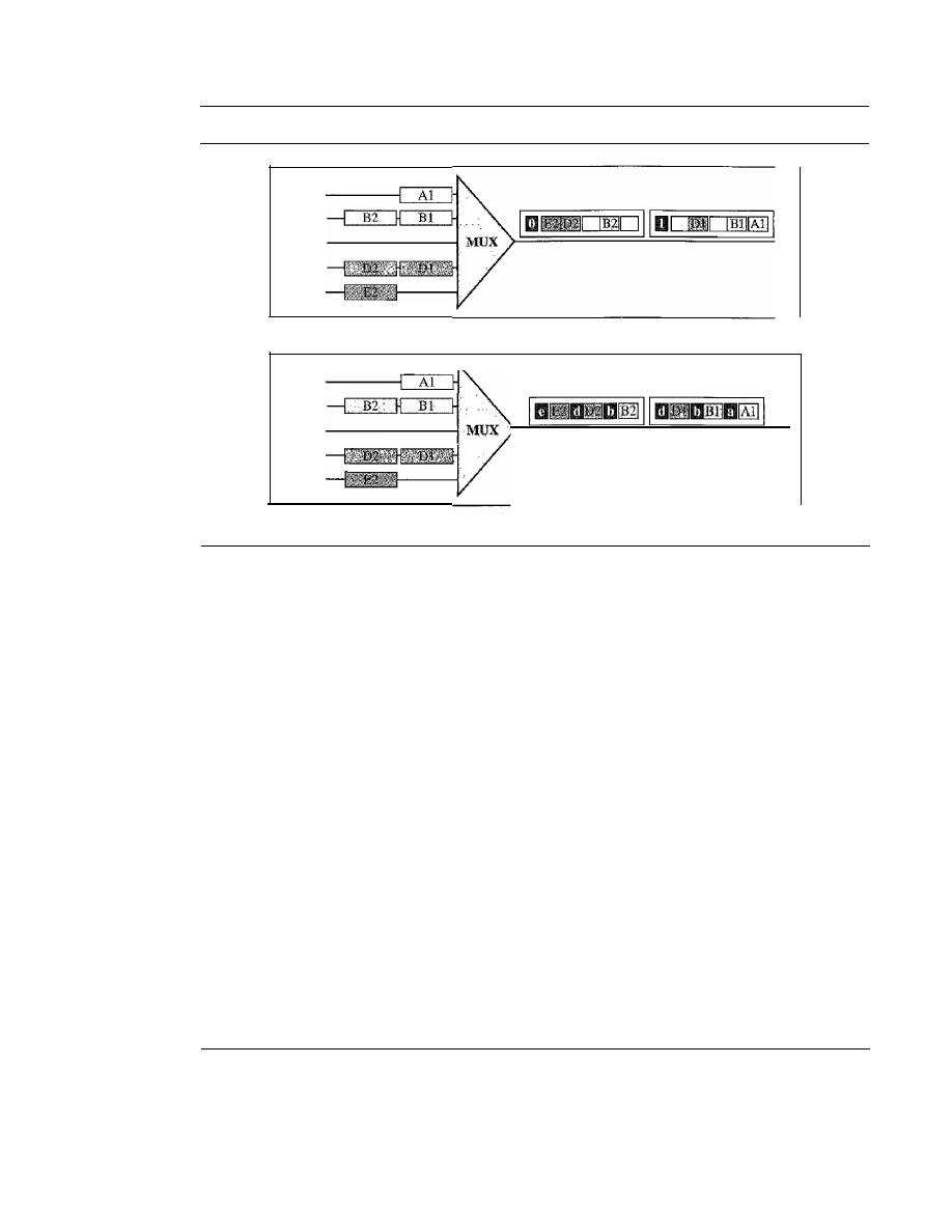
180
CHAPTER
6
BANDWIDTH UTILIZATION: MULTIPLEXING AND SPREADING
Figure 6.26
TDM slot comparison
Line A
LineB
Line C - - - - - - - - {
Line 0
LineE
a. Synchronous TDM
Line A
LineB
Line C
Line 0
LineE
b. Statistical TDM
Slot Size
Since a slot carries both data and an address in statistical TDM, the ratio of the data size
to address size must be reasonable to make transmission efficient. For example, it
would be inefficient to send 1 bit per slot as data when the address is 3 bits. This would
mean an overhead of 300 percent. In statistical TDM, a block of data is usually many
bytes while the address is just a few bytes.
No Synchronization Bit
There is another difference between synchronous and statistical TDM, but this time it is
at the frame level. The frames in statistical TDM need not be synchronized, so we do not
need synchronization bits.
Bandwidth
In statistical TDM, the capacity of the link is normally less than the sum of the capaci-
ties of each channel. The designers of statistical TDM define the capacity of the link
based on the statistics of the load for each channel.
If
on average only
x
percent of the
input slots are filled, the capacity of the link reflects this. Of course, during peak times,
some slots need to wait.
6.2
SPREAD SPECTRUM
Multiplexing combines signals from several sources to achieve bandwidth efficiency; the
available bandwidth of a link is divided between the sources.
In
spread spectrum (88), we
also combine signals from different sources to fit into a larger bandwidth, but our goals
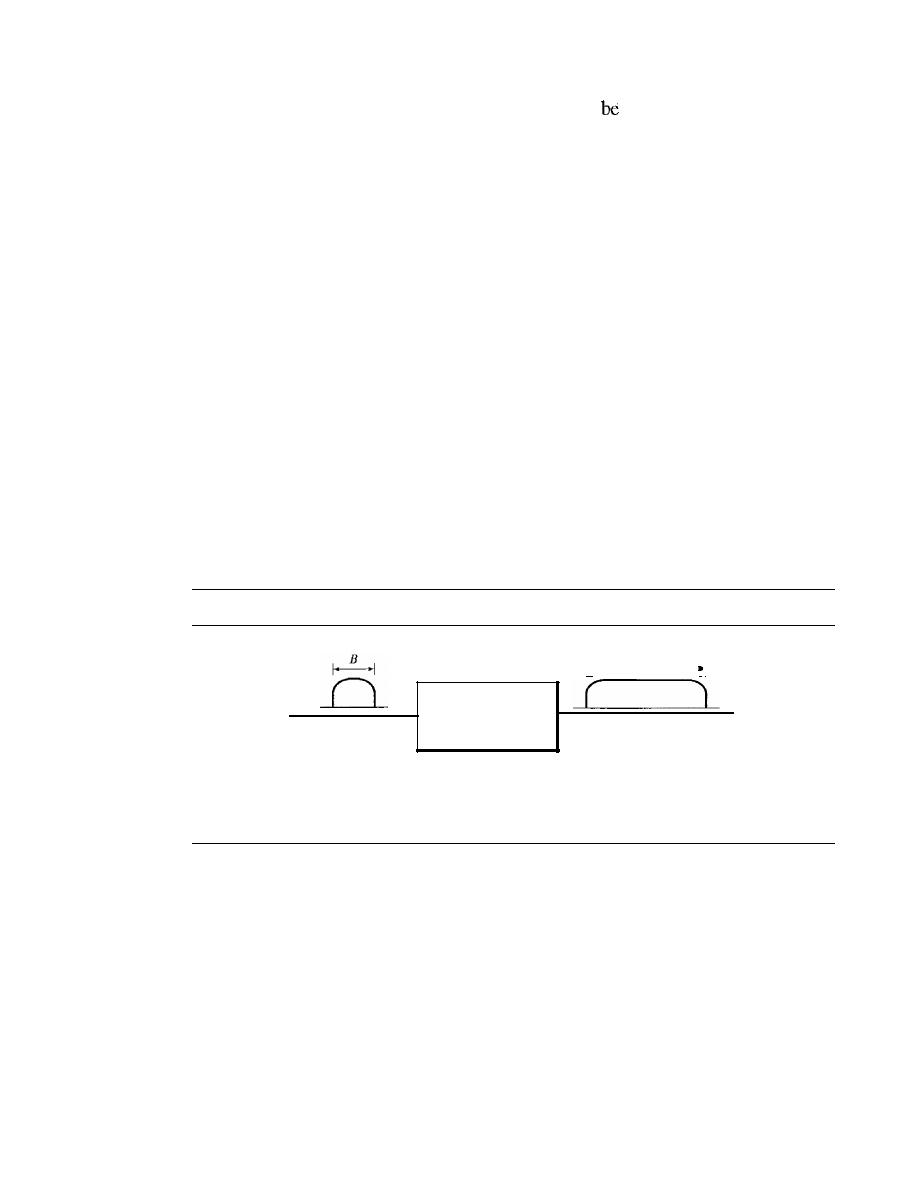
SECTION
6.2
SPREAD SPECTRUM
181
are somewhat different. Spread spectrum is designed to
used in wireless applications
(LANs and WANs). In these types of applications, we have some concerns that outweigh
bandwidth efficiency. In wireless applications, all stations use air (or a vacuum) as the
medium for communication. Stations must be able to share this medium without intercep-
tion by an eavesdropper and without being subject to jamming from a malicious intruder
(in military operations, for example).
To achieve these goals, spread spectrum techniques add redundancy; they spread
the original spectrum needed for each station.
If
the required bandwidth for each station
is
B,
spread spectrum expands it to Bss' such that Bss
»
B.
The expanded bandwidth
allows the source to wrap its message in a protective envelope for a more secure trans-
mission. An analogy is the sending of a delicate, expensive gift. We can insert the gift in
a special box to prevent it from being damaged during transportation, and we can use a
superior delivery service to guarantee the safety of the package.
Figure 6.27 shows the idea of spread spectrum. Spread spectrum achieves its goals
through two principles:
1. The bandwidth allocated to each station needs to be, by far, larger than what is
needed. This allows redundancy.
2. The expanding of the original bandwidth
B
to the bandwidth Bss must be done by a
process that is independent of the original signal. In other words, the spreading
process occurs after the signal is created by the source.
Figure 6.27
Spread spectrum
BSS
I'
I
Spreading
process
i
Spreading
code
After the signal is created by the source, the spreading process uses a spreading
code and spreads the bandwidth. The figure shows the original bandwidth
B
and the
spreaded bandwidth
B
ss.
The spreading code is a series of numbers that look random,
but are actually a pattern.
There are two techniques to spread the bandwidth: frequency hopping spread spec-
trum (FHSS) and direct sequence spread spectrum (DSSS).
Frequency Hopping Spread Spectrum (FHSS)
The frequency hopping spread spectrum (FHSS) technique uses
M
different carrier
frequencies that are modulated by the source signal. At one moment, the signal modu-
lates one carrier frequency; at the next moment, the signal modulates another carrier
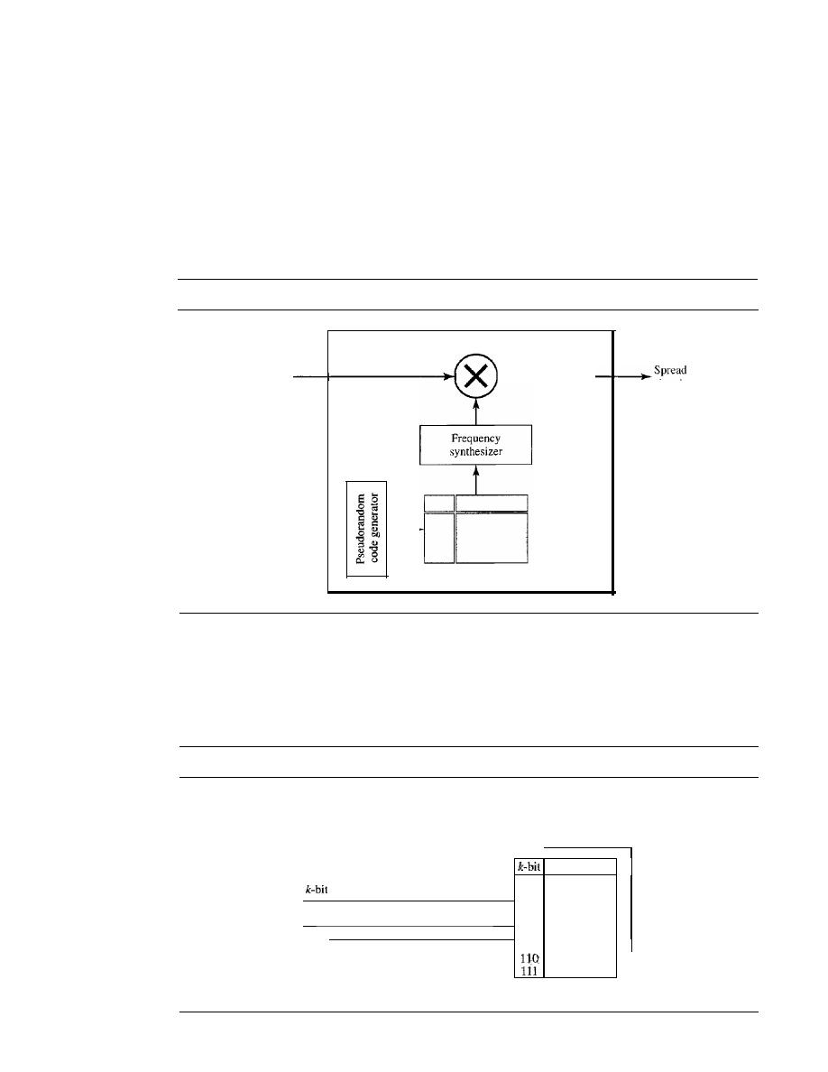
182
CHAPTER
6
BANDWIDTH UTILIZATION: MULTIPLEXING AND SPREADING
frequency. Although the modulation is done using one carrier frequency at a time,
M
frequencies are used in the long run. The bandwidth occupied by a source after
spreading is B
pHSS
»B.
Figure 6.28 shows the general layout for FHSS. A pseudorandom code generator,
called pseudorandom noise (PN), creates a k-bit pattern for every hopping period T
h •
The frequency table uses the pattern to find the frequency to be used for this hopping
period and passes it to the frequency synthesizer. The frequency synthesizer creates a
carrier signal of that frequency, and the source signal modulates the carrier signal.
Figure 6.28
Frequency hopping spread spectrum (FHSS)
Modulator
t -
signal
Original
signal
Frequency table
Suppose we have decided to have eight hopping frequencies. This is extremely low
for real applications and is just for illustration. In this case, Mis 8 and k is 3. The pseudo-
random code generator will create eight different 3-bit patterns. These are mapped to
eight different frequencies in the frequency table (see Figure 6.29).
Figure 6.29
Frequency selection in FHSS
First-hop frequency
t
Frequency
patterns
000
200kHz
001
300kHz
1
101
111 001 000 010 110 011 100
I
010
400kHz
011
500kHz
I
First selection
100
600kHz
101
700kHz-
-
800kHz
900kHz
Frequency table
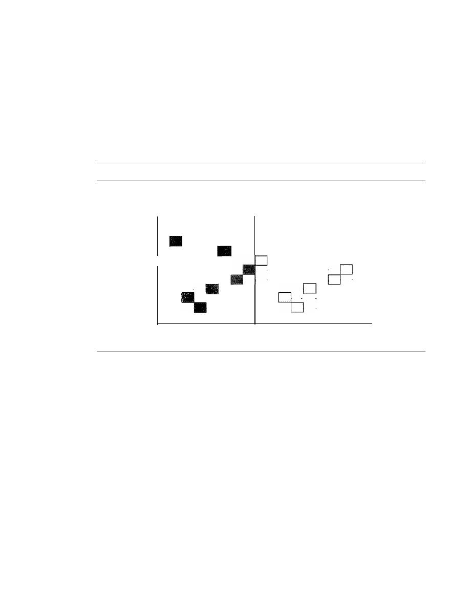
SECTION
6.2
SPREAD SPECTRUM
183
The pattern for this station is 101, 111, 001, 000, 010, all, 100. Note that the pat-
tern is pseudorandom it is repeated after eight hoppings. This means that at hopping
period 1, the pattern is 101. The frequency selected is 700 kHz; the source signal mod-
ulates this carrier frequency. The second k-bit pattern selected is 111, which selects the
900-kHz carrier; the eighth pattern is 100, the frequency is 600 kHz. After eight hop-
pings, the pattern repeats, starting from 101 again. Figure 6.30 shows how the signal hops
around from carrier to carrier. We assume the required bandwidth of the original signal
is 100 kHz.
Figure 6.30
FHSS
cycles
Carrier
frequencies
(kHz)
Cycle 1
D
Cycle
2
D
900
800
700
600
500
400
300
200
1
2
3
4
5
6
7
8
9
10
11
12
13
14
l5
16
Hop
periods
It
can be shown that this scheme can accomplish the previously mentioned goals.
If there are many k-bit patterns and the hopping period is short, a sender and receiver
can have privacy.
If
an intruder tries to intercept the transmitted signal, she can only
access a small piece of data because she does not know the spreading sequence to
quickly adapt herself to the next hop. The scheme has also an antijamming effect. A
malicious sender may be able to send noise to jam the signal for one hopping period
(randomly), but not for the whole period.
Bandwidth Sharing
If the number of hopping frequencies is
M,
we can multiplex
M
channels into one by using
the same B
ss
bandwidth. This is possible because a station uses just one frequency in each
hopping period;
M -
1 other frequencies can be used by other
M -
1 stations. In other
words,
M
different stations can use the same B
ss
if an appropriate modulation technique
such as multiple FSK (MFSK) is used. FHSS is similar to FDM, as shown in Figure 6.31.
Figure 6.31 shows an example of four channels using FDM and four channels
using FHSS. In FDM, each station uses
11M
of the bandwidth, but the allocation is
fixed; in FHSS, each station uses
11M
of the bandwidth, but the allocation changes hop
to hop.
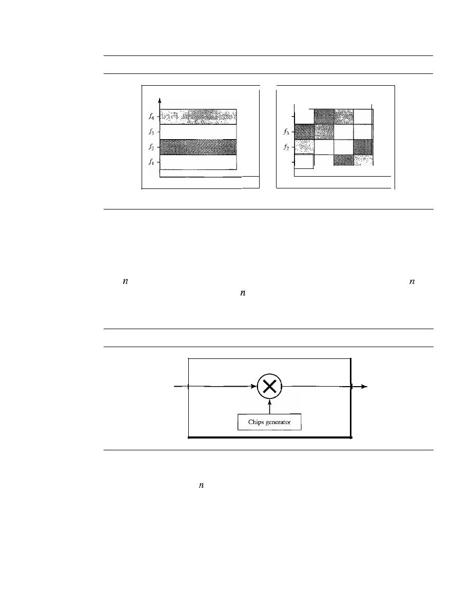
184
CHAPTER
6
BANDWIDTH UTILIZATION: MULTIPLEXING AND SPREADING
Figure 6.31
Bandwidth sharing
Frequency
a.FDM
Frequency
14
f
1
Time
Time
b.FHSS
Direct Sequence Spread Spectrum
The direct sequence spread spectrum
(nSSS)
technique also expands the bandwidth
of the original signal, but the process is different. In DSSS, we replace each data bit
with
bits using a spreading code. In other words, each bit is assigned a code of
bits,
called chips, where the chip rate is
times that of the data bit. Figure 6.32 shows the
concept of DSSS.
Figure 6.32
DSSS
Modulator
Original
signal
Spread
signal
As an example, let us consider the sequence used in a wireless LAN, the famous
Barker sequence where
is 11. We assume that the original signal and the chips in the
chip generator use polar NRZ encoding. Figure 6.33 shows the chips and the result of
multiplying the original data by the chips to get the spread signal.
In Figure 6.33, the spreading code is 11 chips having the pattern 10110111000 (in
this case).
If
the original signal rate is
N, the rate of the spread signal is lIN. This
means that the required bandwidth for the spread signal is 11 times larger than the
bandwidth of the original signal. The spread signal can provide privacy if the intruder
does not know the code.
It
can also provide immunity against interference if each sta-
tion uses a different code.
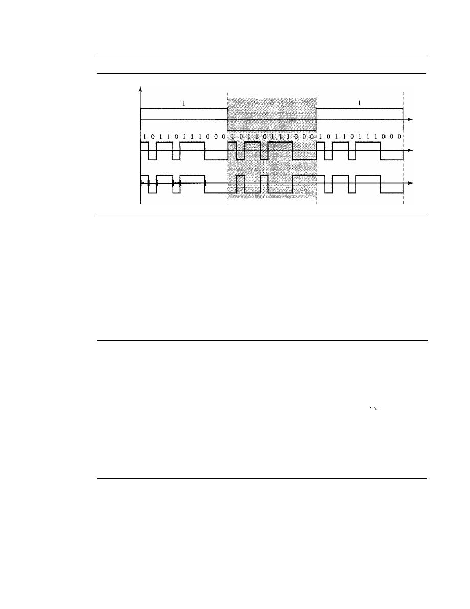
SECTION
6.4
KEY TERMS
185
Figure 6.33
DSSS example
Original
1--
signal
Spreading
code
Spread
signal
Bandwidth Sharing
Can we share a bandwidth in DSSS as we did in FHSS? The answer is no and yes.
If
we
use a spreading code that spreads signals (from different stations) that cannot be combined
and separated, we cannot share a bandwidth. For example, as we will see in Chapter 14,
some wireless LANs use DSSS and the spread bandwidth cannot be shared. However, if
we use a special type of sequence code that allows the combining and separating of spread
signals, we can share the bandwidth. As we will see in Chapter 16, a special spreading code
allows us to use DSSS in cellular telephony and share a bandwidth between several users.
6.3
RECOMMENDED READING
For more details about subjects discussed in this chapter, we recommend the following
books. The items in brackets [...] refer to the reference list at the end of the text.
Books
Multiplexing is elegantly discussed in Chapters 19 of [Pea92]. [CouOI] gives excellent
coverage of TDM and FDM in Sections 3.9 to 3.11. More advanced materials can be
found in [Ber96]. Multiplexing is discussed in Chapter 8 of [Sta04]. A good coverage of
spread spectrum can be found in Section 5.13 of [CouOl] and Chapter 9 of [Sta04].
6.4
KEY TERMS
analog hierarchy
Barker sequence
channel
chip
demultiplexer (DEMUX)
dense WDM (DWDM)
digital signal (DS) service
direct sequence spread spectrum (DSSS)
Eline
framing bit
frequency hopping spread spectrum
(FSSS)

186
CHAPTER
6
BANDWIDTH UTILIZATION: MULTIPLEXING AND SPREADING
frequency-division multiplexing (FDM)
group
guard band
hopping period
interleaving
jumbo group
link
master group
multilevel multiplexing
multiple-slot multiplexing
multiplexer (MUX)
6.5
SUMMARY
multiplexing
pseudorandom code generator
pseudorandom noise (PN)
pulse stuffing
spread spectrum (SS)
statistical TDM
supergroup
synchronous TDM
T line
time-division multiplexing (TDM)
wavelength-division multiplexing (WDM)
o
Bandwidth utilization is the use of available bandwidth to achieve specific goals.
Efficiency can be achieved by using multiplexing; privacy and antijamming can be
achieved by using spreading.
o
Multiplexing is the set of techniques that allows the simultaneous transmission of
multiple signals across a single data link. In a multiplexed system, n lines share the
bandwidth of one link. The word link refers to the physical path. The word channel
refers to the portion of a link that carries a transmission.
o
There are three basic multiplexing techniques: frequency-division multiplexing,
wavelength-division multiplexing, and time-division multiplexing. The first two are
techniques designed for analog signals, the third, for digital signals
o
Frequency-division multiplexing (FDM) is an analog technique that can be applied
when the bandwidth of a link (in hertz) is greater than the combined bandwidths of
the signals to be transmitted.
o
Wavelength-division multiplexing (WDM) is designed to use the high bandwidth
capability of fiber-optic cable. WDM is an analog multiplexing technique to com-
bine optical signals.
o
Time-division multiplexing (TDM) is a digital process that allows several connec-
tions to share the high bandwidth of a link. TDM is a digital multiplexing technique
for combining several low-rate channels into one high-rate one.
o
We can divide TDM into two different schemes: synchronous or statistical. In syn-
chronous TDM, each input connection has an allotment in the output even if it is
not sending data. In statistical TDM, slots are dynamically allocated to improve
bandwidth efficiency.
o
In spread spectrum (SS), we combine signals from different sources to fit into a
larger bandwidth. Spread spectrum is designed to be used in wireless applications
in which stations must be able to share the medium without interception by an
eavesdropper and without being subject to jamming from a malicious intruder.
o
The frequency hopping spread spectrum (FHSS) technique uses M different carrier
frequencies that are modulated by the source signal. At one moment, the signal

SECTION
6.6
PRACTICE SET
187
modulates one carrier frequency; at the next moment, the signal modulates another
carrier frequency.
o
The direct sequence spread spectrum (DSSS) technique expands the bandwidth of
a signal by replacing each data bit with n bits using a spreading code. In other words,
each bit is assigned a code of n bits, called chips.
6.6
PRACTICE SET
Review Questions
1. Describe the goals of multiplexing.
2. List three main multiplexing techniques mentioned in this chapter.
3. Distinguish between a link and a channel in multiplexing.
4. Which of the three multiplexing techniques is (are) used to combine analog signals?
Which of the three multiplexing techniques is (are) used to combine digital signals?
5. Define the analog hierarchy used by telephone companies and list different levels
of the hierarchy.
6. Define the digital hierarchy used by telephone companies and list different levels
of the hierarchy.
7. Which of the three multiplexing techniques is common for fiber optic links?
Explain the reason.
8. Distinguish between multilevel TDM, multiple slot TDM, and pulse-stuffed TDM.
9. Distinguish between synchronous and statistical TDM.
10. Define spread spectrum and its goal. List the two spread spectrum techniques dis-
cussed in this chapter.
11. Define FHSS and explain how it achieves bandwidth spreading.
12. Define DSSS and explain how it achieves bandwidth spreading.
Exercises
13. Assume that a voice channel occupies a bandwidth of 4 kHz. We need to multiplex
10 voice channels with guard bands of 500 Hz using FDM. Calculate the required
bandwidth.
14. We need to transmit 100 digitized voice channels using a pass-band channel of
20 KHz. What should be the ratio of bits/Hz if we use no guard band?
15. In the analog hierarchy of Figure 6.9, find the overhead (extra bandwidth for guard
band or control) in each hierarchy level (group, supergroup, master group, and
jumbo group).
16. We need to use synchronous TDM and combine 20 digital sources, each of 100 Kbps.
Each output slot carries 1 bit from each digital source, but one extra bit is added to
each frame for synchronization. Answer the following questions:
a. What is the size of an output frame in bits?
b. What is the output frame rate?

188
CHAPTER
6
BANDWIDTH UTIUZATION: MULTIPLEXING AND SPREADING
c. What is the duration of an output frame?
d. What is the output data rate?
e. What is the efficiency of the system (ratio of useful bits to the total bits).
17. Repeat Exercise 16 if each output slot carries 2 bits from each source.
18. We have 14 sources, each creating 500 8-bit characters per second. Since only some
of these sources are active at any moment, we use statistical TDM to combine these
sources using character interleaving. Each frame carries 6 slots at a time, but we need
to add four-bit addresses to each slot. Answer the following questions:
a. What is the size of an output frame in bits?
b. What is the output frame rate?
c. What is the duration of an output frame?
d. What is the output data rate?
19. Ten sources, six with a bit rate of 200 kbps and four with a bit rate of 400 kbps are
to be combined using multilevel TDM with no synchronizing bits. Answer the fol-
lowing questions about the final stage of the multiplexing:
a. What is the size of a frame in bits?
b. What is the frame rate?
c. What is the duration of a frame?
d. What is the data rate?
20. Four channels, two with a bit rate of 200 kbps and two with a bit rate of 150 kbps, are
to be multiplexed using multiple slot TDM with no synchronization bits. Answer
the following questions:
a. What is the size of a frame in bits?
b. What is the frame rate?
c. What is the duration of a frame?
d. What is the data rate?
21. Two channels, one with a bit rate of 190 kbps and another with a bit rate of 180 kbps,
are to be multiplexed using pulse stuffing TDM with no synchronization bits. Answer
the following questions:
a. What is the size of a frame in bits?
b. What is the frame rate?
c. What is the duration of a frame?
d. What is the data rate?
22. Answer the following questions about a T-1 line:
a. What is the duration of a frame?
b. What is the overhead (number of extra bits per second)?
23. Show the contents of the five output frames for a synchronous TDM multiplexer
that combines four sources sending the following characters. Note that the characters
are sent in the same order that they are typed. The third source is silent.
a. Source 1 message: HELLO
b. Source 2 message: HI
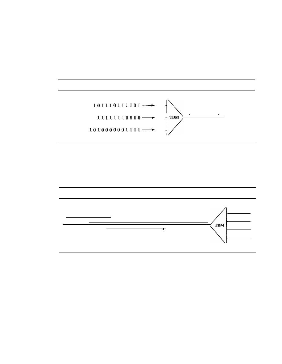
SECTION
6.6
PRACTICE SET
189
c. Source 3 message:
d. Source 4 message: BYE
24. Figure 6.34 shows a multiplexer in a synchronous TDM system. Each output slot is
only 10 bits long (3 bits taken from each input plus 1 framing bit). What is the output
stream? The bits arrive at the multiplexer as shown by the arrows.
Figure 6.34
Exercise 24
I
Frame of 10 bits
I
25. Figure 6.35 shows a demultiplexer in a synchronous TDM. If the input slot is 16 bits
long (no framing bits), what is the bit stream in each output? The bits arrive at the
demultiplexer as shown by the arrows.
Figure 6.35
Exercise 25
101000001110101010101000011101110000011110001
26. Answer the following questions about the digital hierarchy in Figure 6.23:
a. What is the overhead (number of extra bits) in the DS-l service?
b.
What is the overhead (number of extra bits) in the DS-2 service?
c. What is the overhead (number of extra bits) in the DS-3 service?
d. What is the overhead (number of extra bits) in the DS-4 service?
27. What is the minimum number of bits in a PN sequence if we use FHSS with a
channel bandwidth of B
=
4 KHz and B
ss
=
100 KHz?
28. An FHSS system uses a 4-bit PN sequence. If the bit rate of the PN is 64 bits per
second, answer the following questions:
a. What is the total number of possible hops?
b. What is the time needed to finish a complete cycle of PN?

190
CHAPTER
6
BANDWIDTH UTILIZATION: MULTIPLEXING AND SPREADING
29. A pseudorandom number generator uses the following formula to create a random
series:
N
i+
1
=
(5
+
7N
i)
mod
In
which
N
j
defines the current random number and
N
j
+
1
defines the next random
number. The term mod means the value of the remainder when dividing (5
+
7N
j )
by 17.
30. We have a digital medium with a data rate of 10 Mbps. How many 64-kbps voice
channels can be carried by this medium if we use DSSS with the Barker sequence?
CHAPTER 7
Transmission Media
We discussed many issues related to the physical layer in Chapters 3 through 6. In this
chapter, we discuss transmission media. Transmission media are actually located below
the physical layer and are directly controlled by the physical layer. You could say that
transmission media belong to layer zero. Figure 7.1 shows the position of transmission
media in relation to the physical layer.
Figure 7.1
Transmission medium and physical layer
Sender
I
Physical layer
I
Transmission medium
Cable or air
I
Physical layer
I
Receiver
A transmission
medium can be broadly defined as anything that can carry infor-
mation from a source to a destination. For example, the transmission medium for two
people having a dinner conversation is the air. The air can also be used to convey the
message in a smoke signal or semaphore. For a written message, the transmission
medium might be a mail carrier, a truck, or an airplane.
In data communications the definition of the information and the transmission
medium is more specific. The transmission medium is usually free space, metallic cable,
or fiber-optic cable. The information is usually a signal that is the result of a conversion
of data from another form.
The use of long-distance communication using electric signals started with the
invention of the telegraph by Morse in the 19th century. Communication by telegraph
was slow and dependent on a metallic medium.
Extending the range of the human voice became possible when the telephone was
invented in 1869. Telephone communication at that time also needed a metallic medium
to carry the electric signals that were the result of a conversion from the human voice.
191
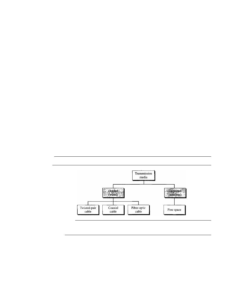
192
CHAPTER
7
1RANSMISSION MEDIA
The communication was, however, unreliable due to the poor quality of the wires. The
lines were often noisy and the technology was unsophisticated.
Wireless communication started in 1895 when Hertz was able to send high-
frequency signals. Later, Marconi devised a method to send telegraph-type messages
over the Atlantic Ocean.
We have come a long way. Better metallic media have been invented (twisted-
pair and coaxial cables, for example). The use of optical fibers has increased the data
rate incredibly. Free space (air, vacuum, and water) is used more efficiently, in part
due to the technologies (such as modulation and multiplexing) discussed in the previous
chapters.
As discussed in Chapter
3,
computers and other telecommunication devices use
signals to represent data. These signals are transmitted from one device to another in the
form of electromagnetic energy, which is propagated through transmission media.
Electromagnetic energy, a combination of electric and magnetic fields vibrating in
relation to each other, includes power, radio waves, infrared light, visible light, ultraviolet
light, and
X,
gamma, and cosmic rays. Each of these constitutes a portion of the electro-
magnetic spectrum. Not all portions of the spectrum are currently usable for telecommu-
nications, however. The media to harness those that are usable are also limited to a few
types.
In telecommunications, transmission media can be divided into two broad catego-
ries: guided and unguided. Guided media include twisted-pair cable, coaxial cable, and
fiber-optic cable. Unguided medium is free space. Figure
7.2
shows this taxonomy.
Figure 7.2
Classes of transmission media
7.1
GUIDED MEDIA
Guided media, which are those that provide a conduit from one device to another,
include twisted-pair cable, coaxial cable, and fiber-optic cable. A signal traveling
along any of these media is directed and contained by the physical limits of the
medium. Twisted-pair and coaxial cable use metallic (copper) conductors that accept
and transport signals in the form of electric current. Optical fiber is a cable that accepts
and transports signals in the form of light.
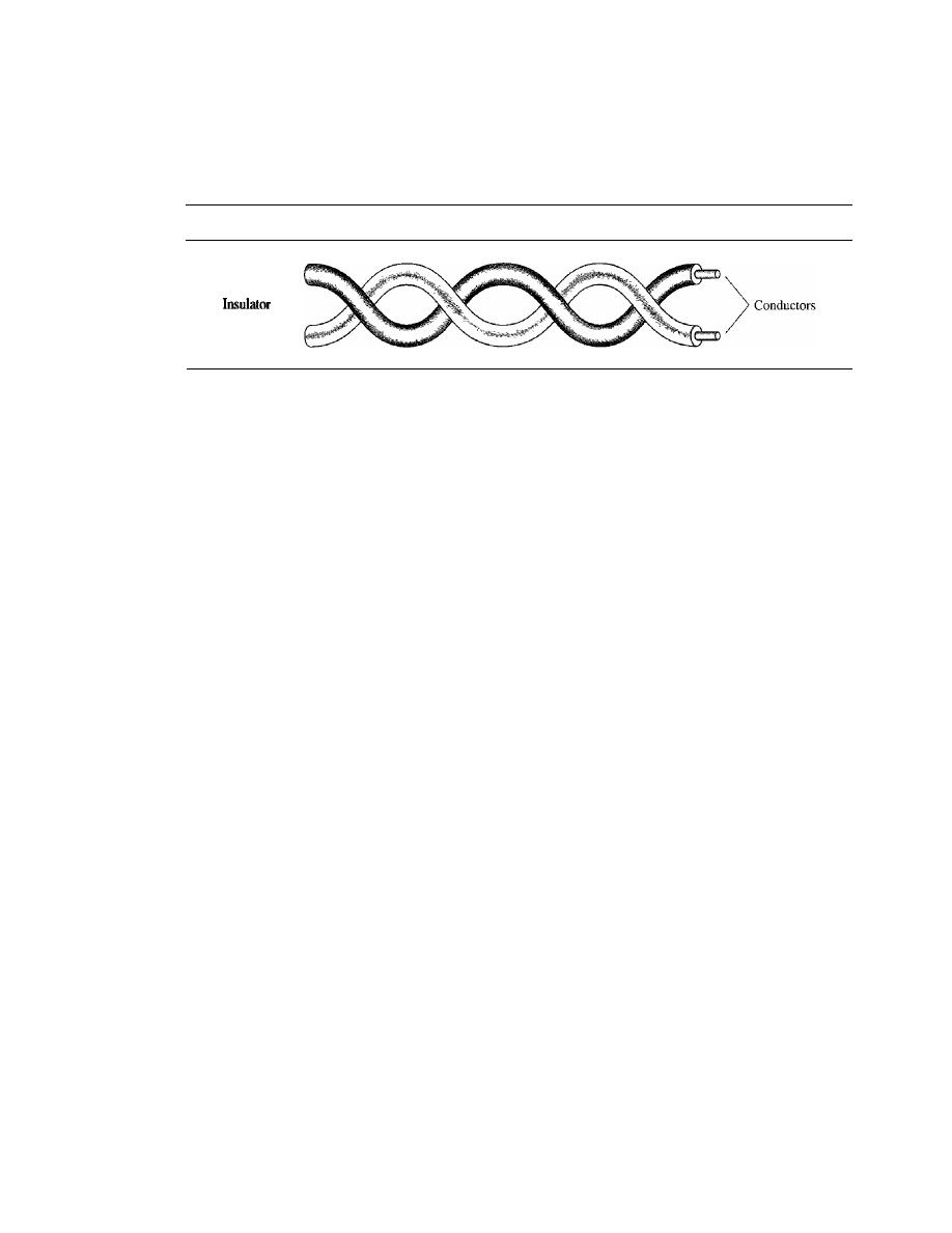
SECTION
7.1
GUIDED MEDIA
193
Twisted-Pair Cable
A twisted pair consists of two conductors (normally copper), each with its own plastic
insulation, twisted together, as shown in Figure 7.3.
Figure 7.3
Twisted-pair cable
<
One of the wires is used to carry signals to the receiver, and the other is used only
as a ground reference. The receiver uses the difference between the two.
In addition to the signal sent by the sender on one of the wires, interference (noise)
and crosstalk may affect both wires and create unwanted signals.
If
the two wires are parallel, the effect of these unwanted signals is not the same in
both wires because they are at different locations relative to the noise or crosstalk sources
(e,g., one is closer and the other is farther). This results in a difference at the receiver. By
twist,ing the pairs, a balance is maintained. For example, suppose in one twist, one wire
is closer to the noise source and the other is farther; in the next twist, the reverse is true.
Twisting makes it probable that both wires are equally affected by external influences
(noise or crosstalk). This means that the receiver, which calculates the difference between
the two, receives no unwanted signals. The unwanted signals are mostly canceled out.
From the above discussion, it is clear that the number of twists per unit of length
(e.g., inch) has some effect on the quality of the cable.
Unshielded Versus Shielded Twisted-Pair Cable
The most common twisted-pair cable used in communications is referred to as
unshielded twisted-pair
(UTP). IBM has also produced a version of twisted-pair cable
for its use called
shielded twisted-pair
(STP). STP cable has a metal foil or braided-
mesh covering that encases each pair of insulated conductors. Although metal casing
improves the quality of cable by preventing the penetration of noise or crosstalk, it is
bulkier and more expensive. Figure 7.4 shows the difference between UTP and STP.
Our discussion focuses primarily on UTP because STP is seldom used outside of IBM.
Categories
The Electronic Industries Association (EIA) has developed standards to classify
unshielded twisted-pair cable into seven categories. Categories are determined by cable
quality, with 1 as the lowest and 7 as the highest. Each EIA category is suitable for
specific uses. Table 7. I shows these categories.
Connectors
The most common UTP connector is RJ45 (RJ stands for registered jack), as shown
in Figure 7.5. The RJ45 is a keyed connector, meaning the connector can be inserted in
only one way.
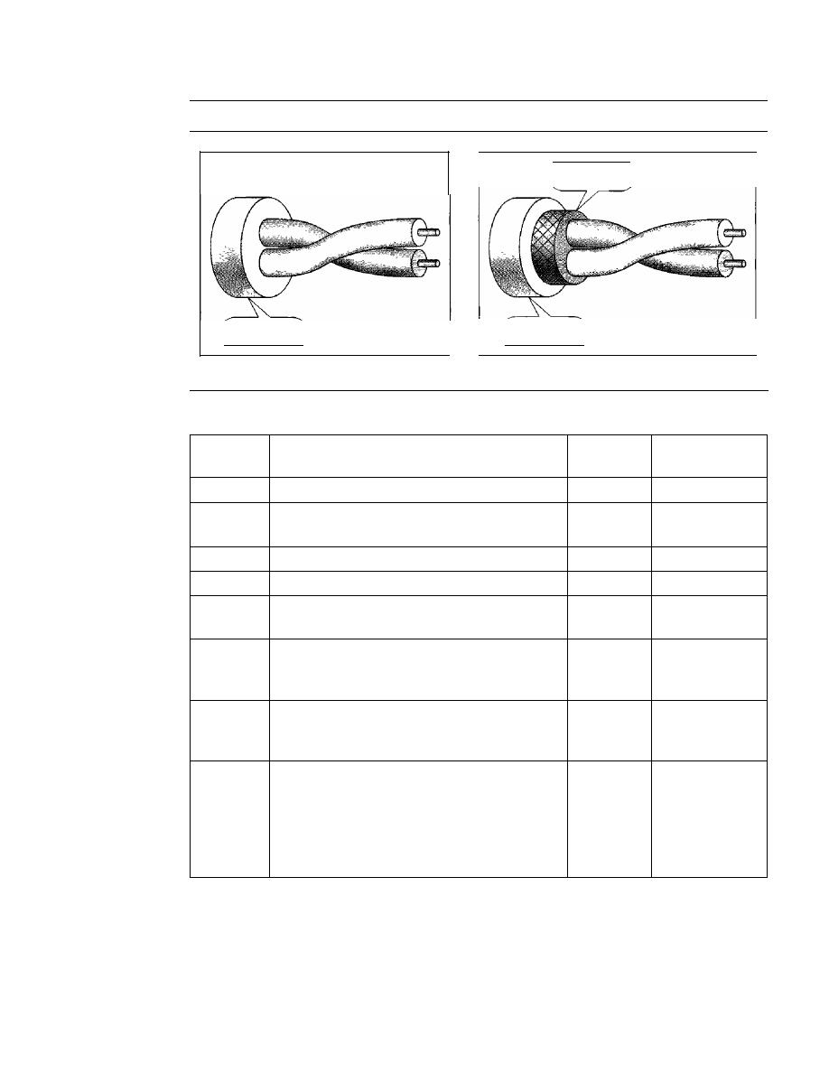
194
CHAPTER
7
TRANSMISSION MEDIA
Figure 7.4
UTP and STP cables
Metal shield
Plastic cover
a.UTP
Plastic cover
b.STP
Table 7.1
Categories of unshielded twisted-pair cables
Data Rate
Category
Specification
(Mbps)
Use
I
Unshielded twisted-pair used in telephone
<
0.1
Telephone
2
Unshielded twisted-pair originally used in
2
T-llines
T-lines
3
Improved CAT 2 used in LANs
10
LANs
4
Improved CAT 3 used in Token Ring networks
20
LANs
5
Cable wire is normally 24 AWG with a jacket
100
LANs
and outside sheath
SE
An extension to category 5 that includes
125
LANs
extra features to minimize the crosstalk and
electromagnetic interference
6
A new category with matched components
200
LANs
coming from the same manufacturer. The
cable must be tested at a 200-Mbps data rate.
7
Sometimes called SSTP (shielded screen
600
LANs
twisted-pair). Each pair is individually
wrapped in a helical metallic foil followed by
a metallic foil shield in addition to the outside
sheath. The shield decreases the effect of
crosstalk: and increases the data rate.
Performance
One way to measure the performance of twisted-pair cable is to compare attenuation
versus frequency and distance. A twisted-pair cable can pass a wide range of frequencies.
However, Figure 7.6 shows that with increasing frequency, the attenuation, measured in
decibels per kilometer (dB/km), sharply increases with frequencies above 100 kHz. Note
that
gauge
is a measure of the thickness of the wire.
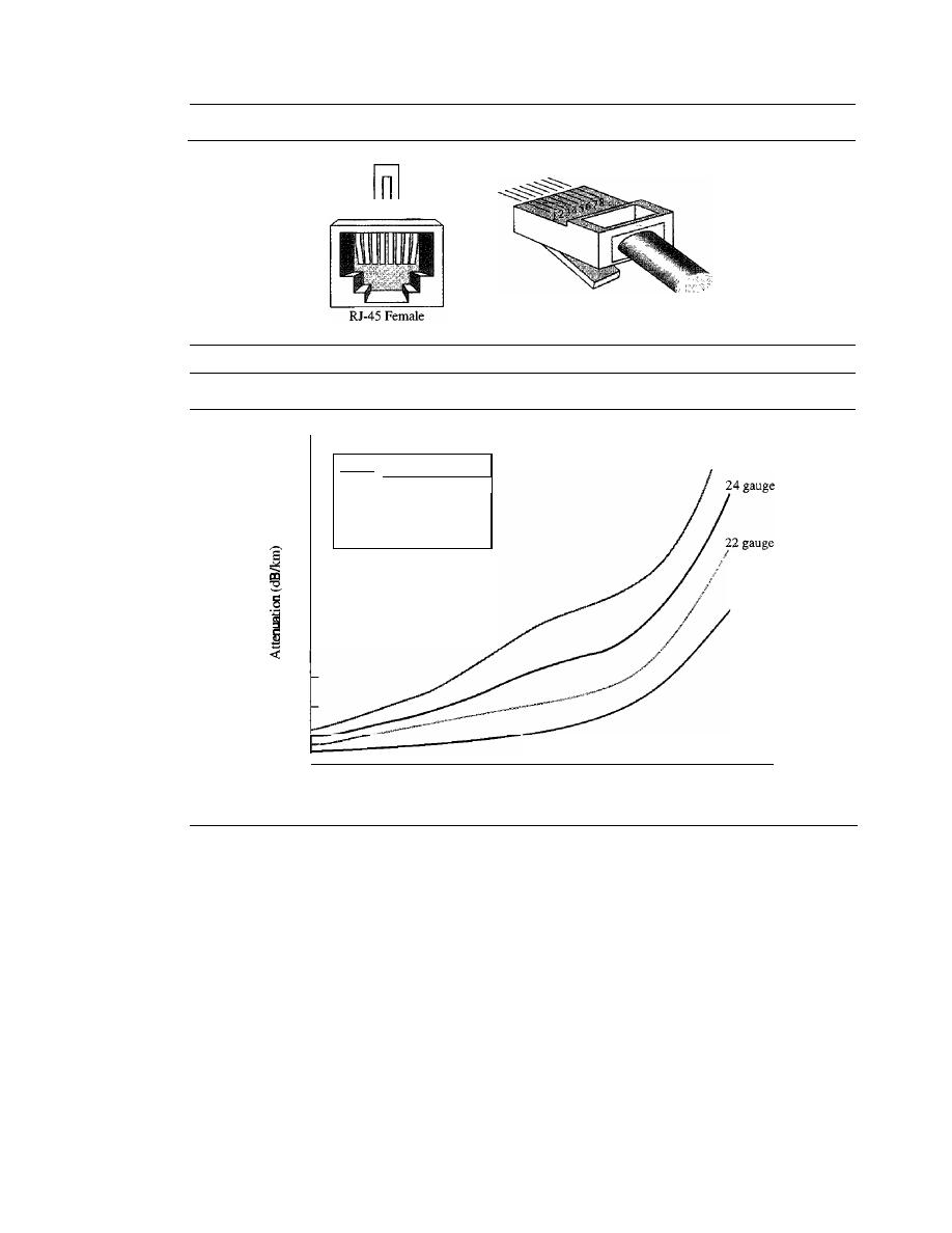
SECTION
7.1
GUIDED MEDIA
195
Figure 7.5
UTP
connector
n n
12345678
RJ-45 Male
Figure 7.6
UTP
performance
18 gauge
26 gauge
Gauge
Diameter (inches)
18
0.0403
22
0.02320
24
0.02010
26
0.0159
18
2
4
20
16
14
12
10
8
6
10
100
1000
!(kHz)
Applications
Twisted-pair cables are used in telephone lines to provide voice and data channels. The
local loop-the line that connects subscribers to the central telephone office---commonly
consists of unshielded twisted-pair cables. We discuss telephone networks in Chapter 9.
The DSL lines that are used by the telephone companies to provide high-data-rate
connections also use the high-bandwidth capability of unshielded twisted-pair cables.
We discuss DSL technology in Chapter 9.
Local-area networks, such as lOBase-T and lOOBase-T, also use twisted-pair cables.
We discuss these networks in Chapter 13.
Coaxial Cable
Coaxial cable (or
coax)
carries signals of higher frequency ranges than those in twisted-
pair cable, in part because the two media are constructed quite differently. Instead of
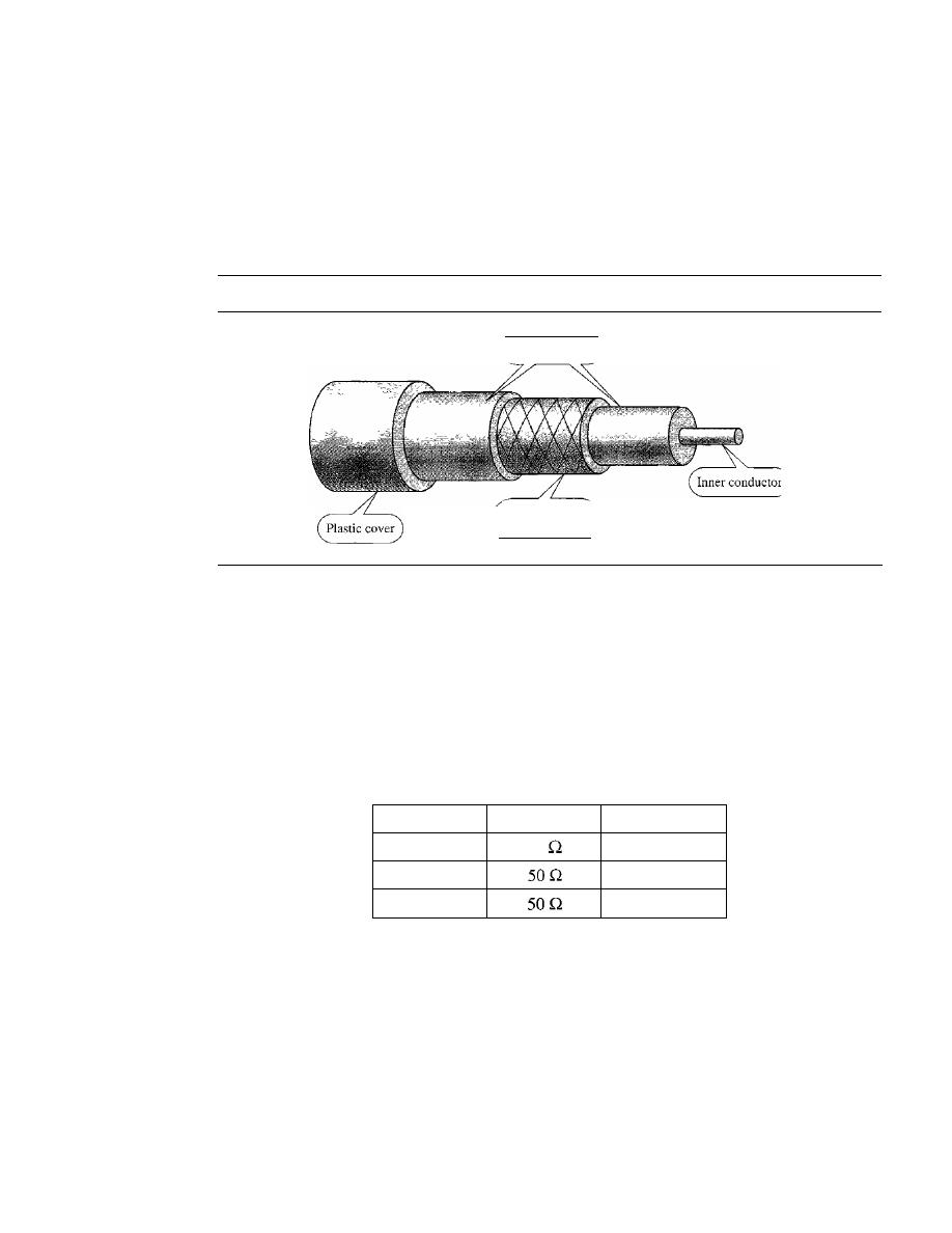
196
CHAPTER
7
TRANSMISSION MEDIA
having two wires, coax has a central core conductor of solid or stranded wire (usually
copper) enclosed in an insulating sheath, which is, in turn, encased in an outer conductor
of metal foil, braid, or a combination of the two. The outer metallic wrapping serves
both as a shield against noise and as the second conductor, which completes the circuit.
This outer conductor is also enclosed in an insulating sheath, and the whole cable is
protected by a plastic cover (see Figure 7.7).
Figure 7.7
Coaxial cable
Insulator
Outer conductor
(shield)
Coaxial Cable Standards
Coaxial cables are categorized by their
radio government (RG)
ratings. Each RG num-
ber denotes a unique set of physical specifications, including the wire gauge of the
inner conductor, the thickness and type of the inner insulator, the construction of the
shield, and the size and type of the outer casing. Each cable defined by an RG rating is
adapted for a specialized function, as shown in Table 7.2.
Table
7.2
Categories of coaxial cables
Category
Impedance
Use
RG-59
75
Cable TV
RG-58
Thin Ethernet
RG-ll
Thick Ethernet
Coaxial Cable Connectors
To connect coaxial cable to devices, we need coaxial connectors. The most common
type of connector used today is the
Bayone-Neill-Concelman (BNe),
connector.
Figure 7.8 shows three popular types of these connectors: the BNC connector, the
BNC T connector, and the BNC terminator.
The BNC connector is used to connect the end of the cable to a device, such as a
TV set. The BNC T connector is used in Ethernet networks (see Chapter 13) to branch
out to a connection to a computer or other device. The BNC terminator is used at the
end of the cable to prevent the reflection of the signal.
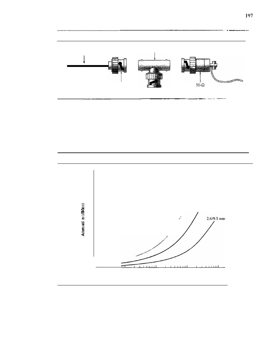
SECTION
7.1
GUIDED MEDIA
Figure 7.8
BNC connectors
BNCT
Cable
BNC
connector
BNe
terminator
Ground
wire
Performance
As we did with twisted-pair cables, we can measure the performance of a coaxial cable.
We notice in Figure 7.9 that the attenuation is much higher in coaxial cables than in
twisted-pair cable. In other words, although coaxial cable has a much higher bandwidth,
the signal weakens rapidly and requires the frequent use of repeaters.
Figure 7.9
Coaxial cable peiformance
100
IO
0.712.9
mm
!
/
I
/
1.2/4.4
mm
!
/
1.0
j(kHz)
0.1
35
30
25
20
0
15
10
5
0.01
Applications
Coaxial cable was widely used in analog telephone networks where a single coaxial net-
work could carry 10,000 voice signals. Later it was used in digital telephone networks
where a single coaxial cable could carry digital data up to 600 Mbps. However, coaxial
cable in telephone networks has largely been replaced today with fiber-optic cable.
Cable TV networks (see Chapter 9) also use coaxial cables. In the traditional cable
TV network, the entire network used coaxial cable. Later, however, cable TV providers
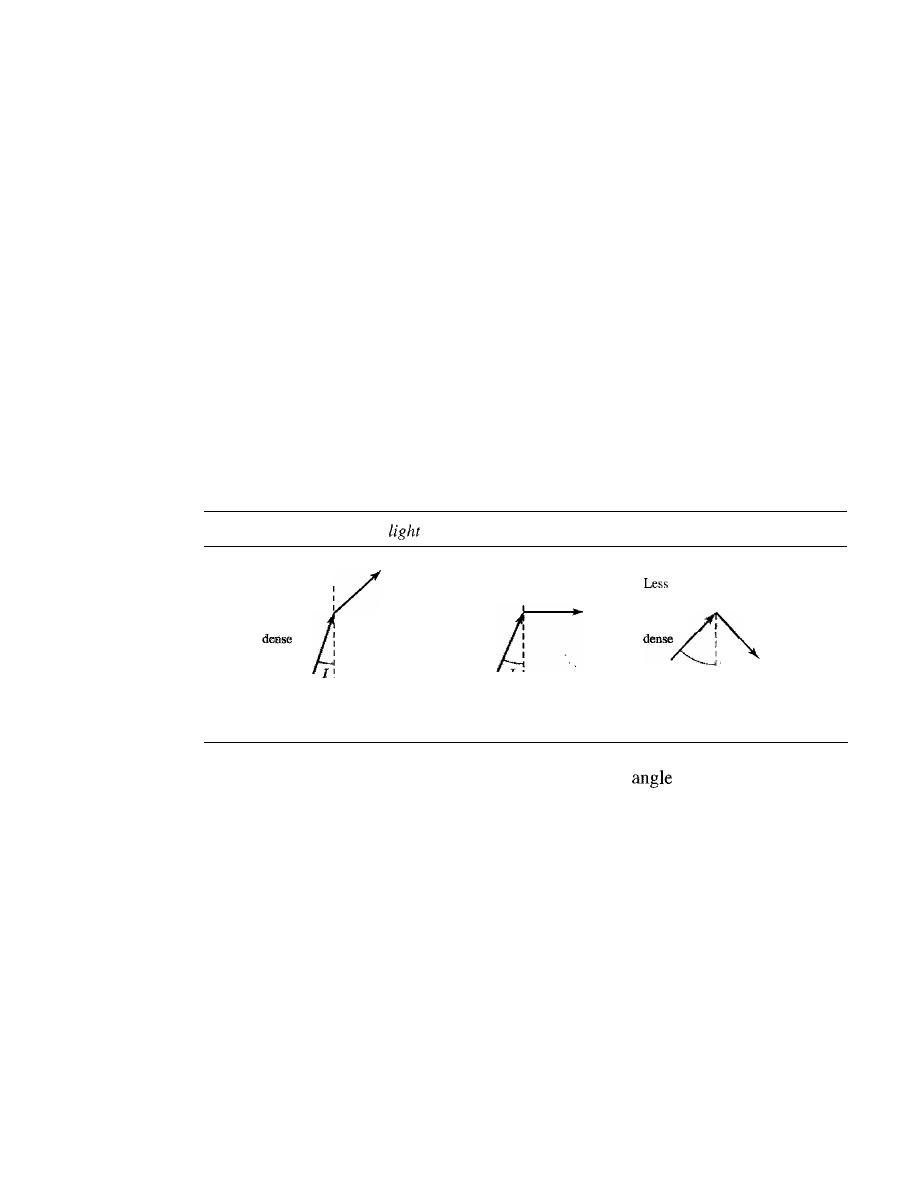
198
CHAPTER
7
TRANSMISSION MEDIA
replaced most of the media with fiber-optic cable; hybrid networks use coaxial cable
only at the network boundaries, near the consumer premises. Cable TV uses RG-59
coaxial cable.
Another common application of coaxial cable is in traditional Ethernet LANs (see
Chapter 13). Because of its high bandwidth, and consequently high data rate, coaxial
cable was chosen for digital transmission in early Ethernet LANs. The 10Base-2, or Thin
Ethernet, uses RG-58 coaxial cable with BNe connectors to transmit data at 10 Mbps
with a range of 185 m. The lOBase5, or Thick Ethernet, uses RG-11 (thick coaxial cable)
to transmit 10 Mbps with a range of 5000 m. Thick Ethernet has specialized connectors.
Fiber-Optic Cable
A fiber-optic cable is made of glass or plastic and transmits signals in the form of light.
To understand optical fiber, we first need to explore several aspects of the nature of light.
Light travels
in
a straight line as long as it is moving through a single uniform sub-
stance. If a ray of light traveling through one substance suddenly enters another substance
(of a different density), the ray changes direction. Figure 7.10 shows how a ray of light
changes direction when going from a more dense to a less dense substance.
Figure 7.10
Bending of
ray
Less
dense
More
More
dense
Less
dense
I>
critical angle,
reflection
dense
I
I
I
More,
[
I
I
I
I
I
I
I
I
=
critical angle,
refraction
I
I
<
critical angle,
refraction
As the figure shows, if the angle of incidence
I
(the
the ray makes with the
line perpendicular to the interface between the two substances) is less than the critical
angle, the ray refracts and moves closer to the surface.
If
the angle of incidence is
equal to the critical angle, the light bends along the interface.
If
the angle is greater than
the critical angle, the ray reflects (makes a turn) and travels again in the denser sub-
stance. Note that the critical angle is a property of the substance, and its value differs
from one substance to another.
Optical fibers use reflection to guide light through a channel. A glass or plastic core
is surrounded by a cladding of less dense glass or plastic. The difference in density of the
two materials must be such that a beam of light moving through the core is reflected off
the cladding instead of being refracted into it. See Figure 7.11.
Propagation Modes
Current technology supports two modes (multimode and single mode) for propagating light
along optical channels, each requiring fiber with different physical characteristics. Multi-
mode can be implemented in two forms: step-index or graded-index (see Figure 7.12).
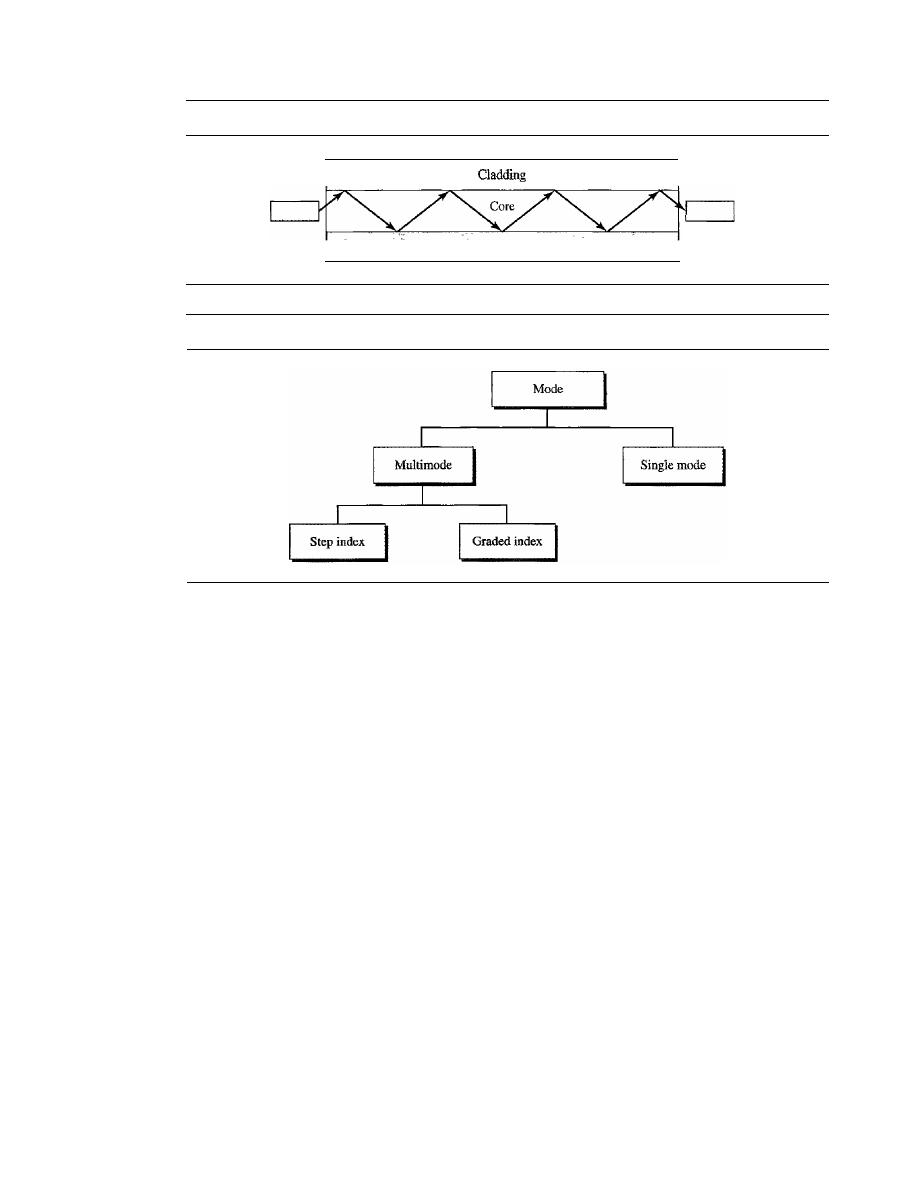
SECTION
7.1
GUlDED MEDIA
199
Figure 7.11
Opticaljiber
Sender
Figure 7.12
Propagation modes
Cladding
Receiver
Multimode
Multimode is so named because multiple beams from a light source
move through the core in different paths. How these beams move within the cable
depends on the structure ofthe core, as shown in Figure 7.13.
In multimode step-index fiber, the density of the core remains constant from the
center to the edges. A beam of light moves through this constant density in a straight
line until it reaches the interface of the core and the cladding. At the interface, there is
an abrupt change due to a lower density; this alters the angle of the beam's motion. The
term step index refers to the suddenness of this change, which contributes to the distor-
tion of the signal as it passes through the fiber.
A second type of fiber, called multimode graded-index fiber, decreases this distor-
tion of the signal through the cable. The word index here refers to the index of refraction.
As we saw above, the index of refraction is related to density. A graded-index fiber,
therefore, is one with varying densities. Density is highest at the center of the core and
decreases gradually to its lowest at the edge. Figure 7.13 shows the impact of this vari-
able density on the propagation of light beams.
Single-Mode
Single-mode uses step-index fiber and a highly focused source of light
that limits beams to a small range of angles, all close to the horizontal. The single-
mode fiber itself is manufactured with a much smaller diameter than that of multimode
fiber, and with substantiallY lower density (index of refraction). The decrease in density
results in a critical angle that is close enough to 90° to make the propagation of beams
almost horizontal. In this case, propagation of different beams is almost identical, and
delays are negligible. All the beams arrive at the destination "together" and can be
recombined with little distortion to the signal (see Figure 7.13).
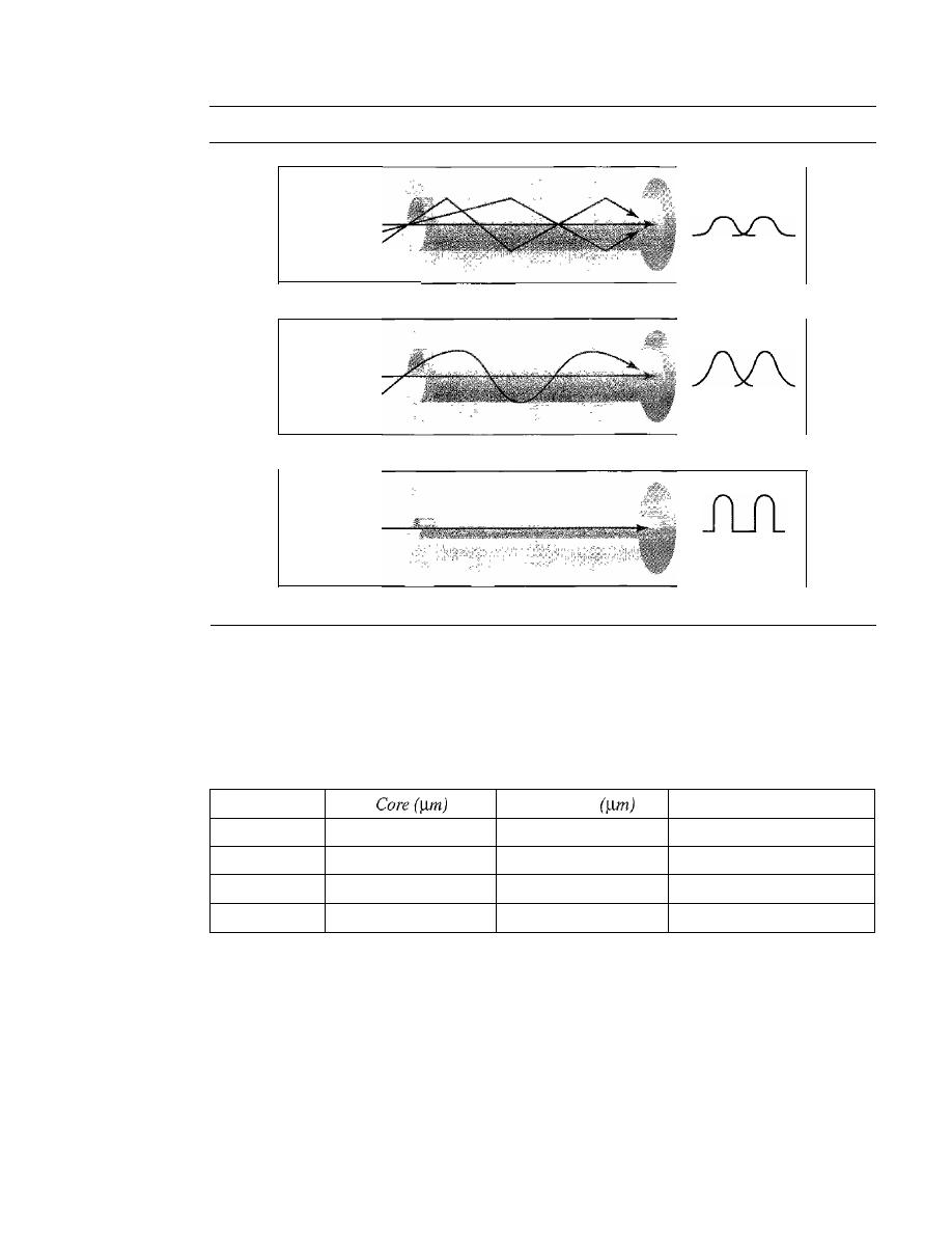
200
CHAPTER
7
TRANSMISSION MEDIA
Figure 7.13
Modes
JlJ1
Source
a. Multimode, step index
Destination
JlJ1
Source
Destination
b. Multimode, graded index
JlJ1
Source
c. Single mode
Destination
Fiber Sizes
Optical fibers are defined by the ratio of the diameter of their core to the diameter of
their cladding, both expressed in micrometers. The common sizes are shown in Table 7.3.
Note that the last size listed is for single-mode only.
Table 7.3
Fiber types
Type
Cladding
Mode
501125
50.0
125
Multimode, graded index
62.51125
62.5
125
Multimode, graded index
100/125
100.0
125
Multimode, graded index
7/125
7.0
125
Single mode
Cable Composition
Figure 7.14 shows the composition of a typical fiber-optic cable. The outer jacket is made
of either PVC or Teflon. Inside the jacket are Kevlar strands to strengthen the cable. Kevlar
is a strong material used in the fabrication of bulletproof vests. Below the Kevlar is another
plastic coating to cushion the fiber. The fiber is at the center of the cable, and it consists of
cladding and core.
Fiber-Optic Cable Connectors
There are three types of connectors for fiber-optic cables, as shown in Figure 7.15.
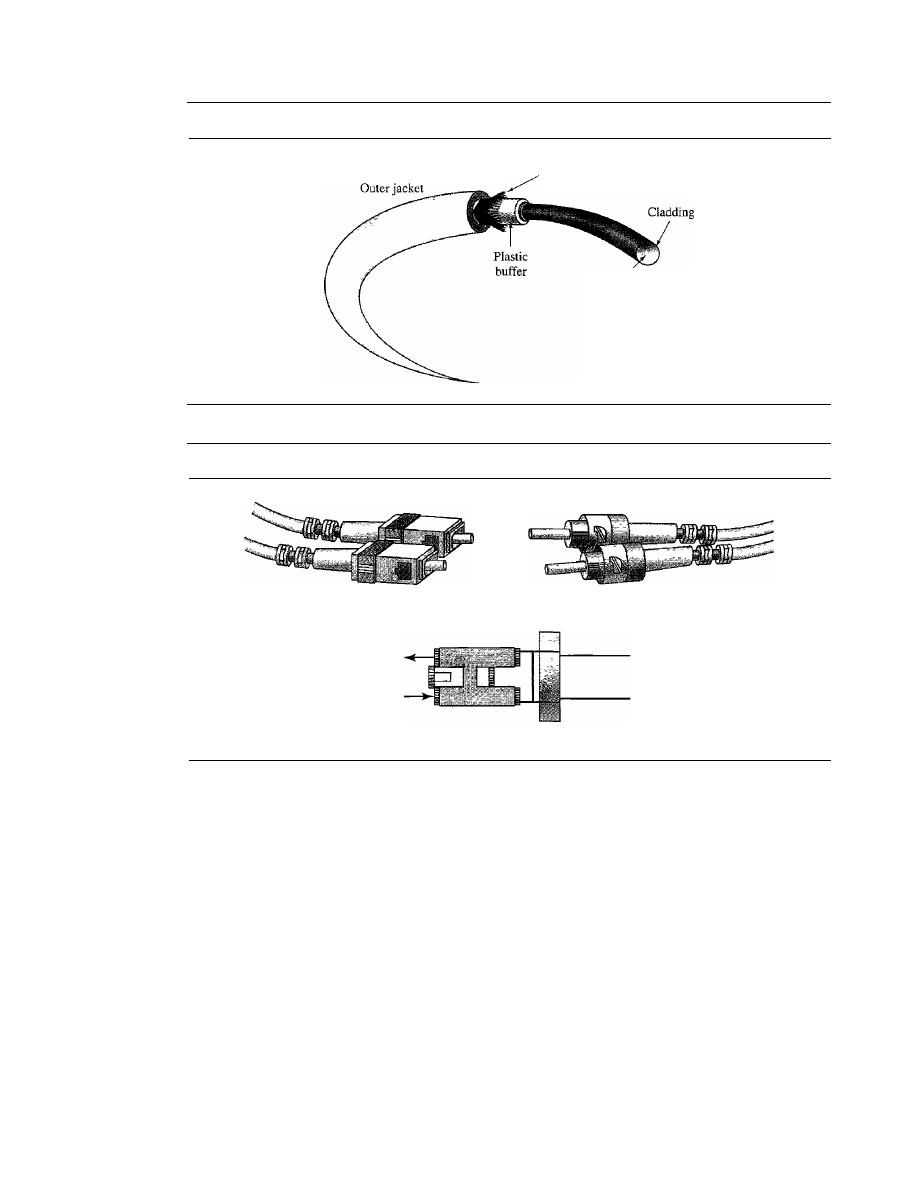
SECTION
7.1
GUIDED MEDIA
201
Figure 7.14
Fiber construction
Du Pont Kevlar
for strength
Glass or
plastic core
Figure 7.15
Fiber-optic cable connectors
SC connector
ST connector
RX
TX
MT-RJ connector
The
subscriber channel
(SC)
connector
is used for cable TV.
It
uses a push/pull
locking system. The
straight-tip
(ST)
connector
is used for connecting cable to
networking devices.
It
uses a bayonet locking system and is more reliable than SC.
MT-RJ
is a connector that is the same size as RJ45.
Performance
The plot of attenuation versus wavelength in Figure 7.16 shows a very interesting
phenomenon in fiber-optic cable. Attenuation is flatter than in the case of twisted-pair
cable and coaxial cable. The performance is such that we need fewer (actually 10 times
less) repeaters when we use fiber-optic cable.
Applications
Fiber-optic cable is often found in backbone networks because its wide bandwidth is
cost-effective. Today, with wavelength-division multiplexing (WDM), we can transfer
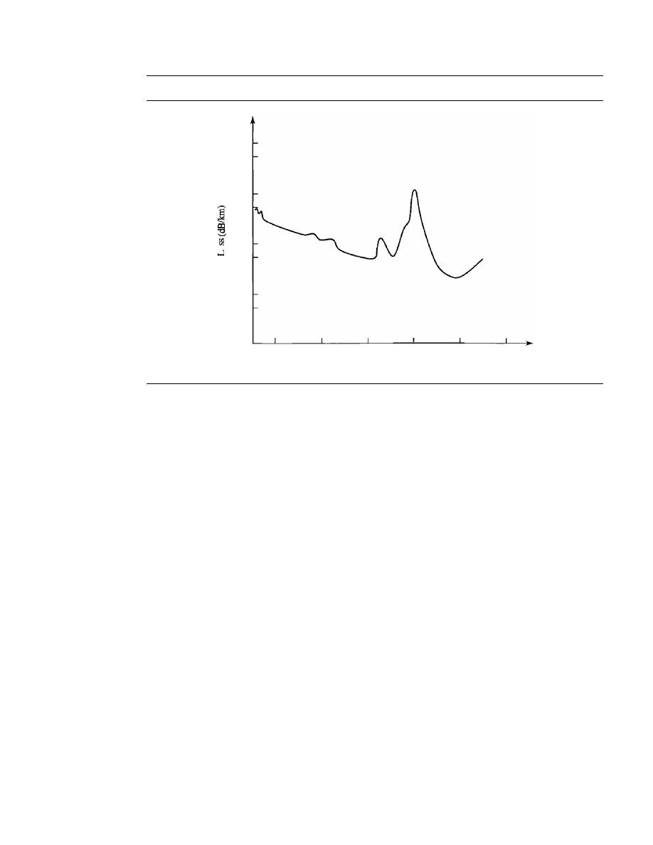
202
CHAPTER
7
IRANSMISSION MEDIA
Figure 7.16
Optical fiber performance
100
50
IO
5
1
0
0.5
0.1
0.05
0.01
800
1000
1200
1400
1600
1800
Wavelength (urn)
data at a rate of 1600 Gbps. The SONET network that we discuss in Chapter 17 provides
such a backbone.
Some cable TV companies use a combination of optical fiber and coaxial cable,
thus creating a hybrid network. Optical fiber provides the backbone structure while
coaxial cable provides the connection to the user premises. This is a cost-effective con-
figuration since the narrow bandwidth requirement at the user end does not justify the
use of optical fiber.
Local-area networks such as 100Base-FX network (Fast Ethernet) and 1000Base-X
also use fiber-optic cable.
Advantages and Disadvantages of Optical Fiber
Advantages
Fiber-optic cable has several advantages over metallic cable (twisted-
pair or coaxial).
D
Higher bandwidth. Fiber-optic cable can support dramatically higher bandwidths
(and hence data rates) than either twisted-pair or coaxial cable. Currently, data rates
and bandwidth utilization over fiber-optic cable are limited not by the medium but
by the signal generation and reception technology available.
D
Less signal attenuation. Fiber-optic transmission distance is significantly greater
than that of other guided media. A signal can run for 50 km without requiring
regeneration. We need repeaters every 5
km
for coaxial or twisted-pair cable.
D
Immunity to electromagnetic interference. Electromagnetic noise cannot affect
fiber-optic cables.
o
Resistance to corrosive materials. Glass is more resistant to corrosive materials
than copper.

SECTION 7.2
UNGUIDED MEDIA: WIRELESS
203
o
Light weight. Fiber-optic cables are much lighter than copper cables.
o
Greater immunity to tapping. Fiber-optic cables are more immune to tapping than
copper cables. Copper cables create antenna effects that can easily be tapped.
Disadvantages
There are some disadvantages in the use of optical fiber.
o
Installation and maintenance. Fiber-optic cable is a relatively new technology. Its
installation and maintenance require expertise that is not yet available everywhere.
o
Unidirectional light propagation. Propagation of light is unidirectional.
If
we
need bidirectional communication, two fibers are needed.
o
Cost. The cable and the interfaces are relatively more expensive than those of other
guided media.
If
the demand for bandwidth is not high, often the use of optical fiber
cannot be justified.
7.2
UNGUIDED MEDIA: WIRELESS
Unguided media transport electromagnetic waves without using a physical conductor.
This type of communication is often referred to as wireless communication. Signals
are normally broadcast through free space and thus are available to anyone who has a
device capable of receiving them.
Figure 7.17 shows the part of the electromagnetic spectrum, ranging from 3 kHz to
900 THz, used for wireless communication.
Figure 7.17
Electromagnetic spectrumfor wireless communication
3
kHz
Radio wave and microwave
300
400
900
GHz
THz THz
Unguided signals can travel from the source to destination in several ways: ground
propagation, sky propagation, and line-of-sight propagation, as shown in Figure 7.18.
In ground propagation, radio waves travel through the lowest portion of the
atmosphere, hugging the earth. These low-frequency signals emanate in all directions
from the transmitting antenna and follow the curvature of the planet. Distance depends
on the amount of power in the signal: The greater the power, the greater the distance. In
sky propagation, higher-frequency radio waves radiate upward into the ionosphere
(the layer of atmosphere where particles exist as ions) where they are reflected back to
earth. This type of transmission allows for greater distances with lower output power.
In line-or-sight propagation, very high-frequency signals are transmitted in straight
lines directly from antenna to antenna. Antennas must be directional, facing each other,
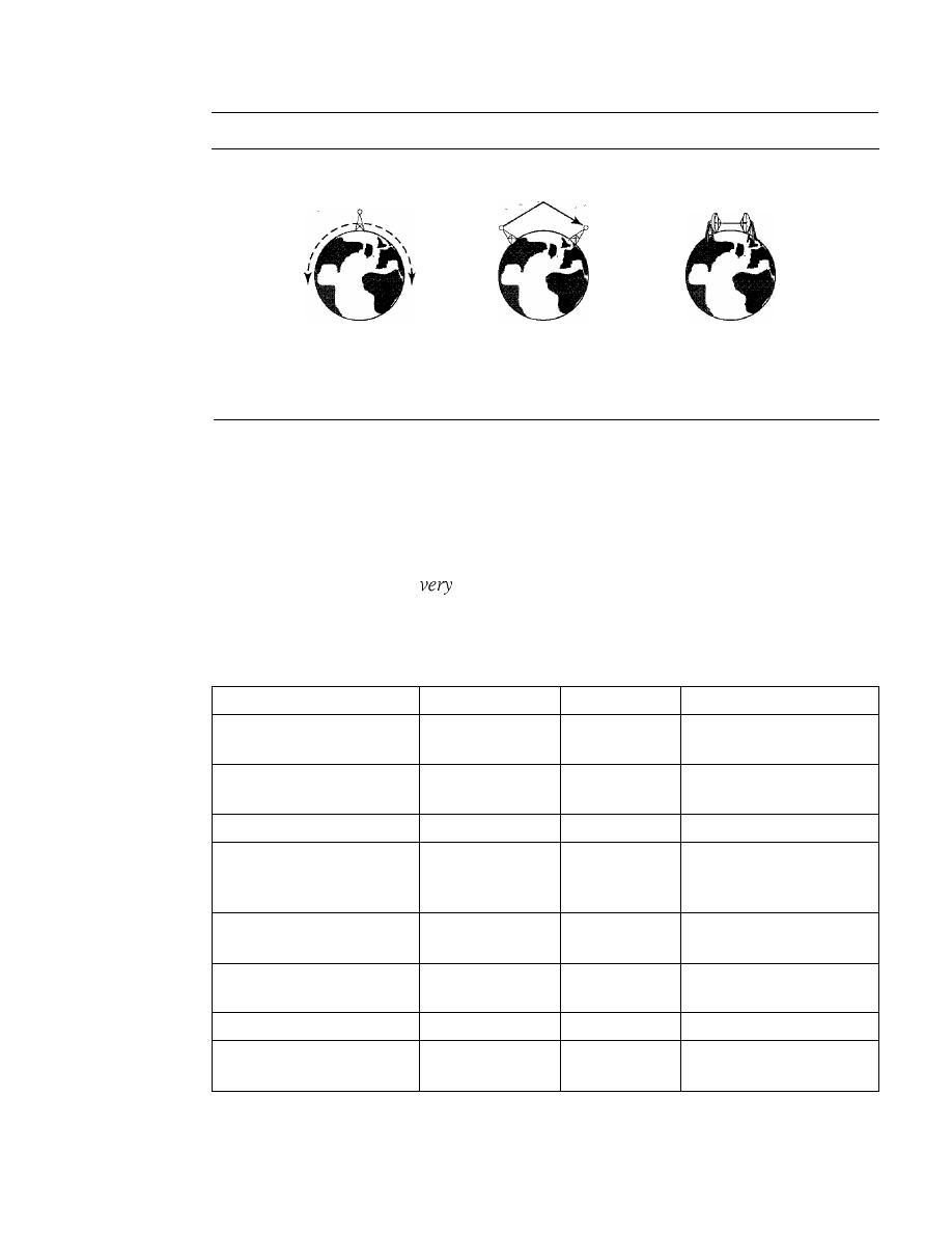
204
CHAPTER
7
TRANSMISSION MEDIA
Figure 7.18
Propagation methods
Ionosphere
Ground propagation
(below 2 MHz)
Ionosphere
Sky
propagation
(2-30 MHz)
Ionosphere
Line-af-sight propagation
(above
30 MHz)
and either tall enough or close enough together not to be affected by the curvature of
the earth. Line-of-sight propagation is tricky because radio transmissions cannot be
completely focused.
The section of the electromagnetic spectrum defined as radio waves and microwaves
is divided into eight ranges, called bands, each regulated by government authorities.
These bands are rated from
low frequency
(VLF) to extremely highfrequency (EHF).
Table 7.4 lists these bands, their ranges, propagation methods, and some applications.
Table
7.4
Bands
Band
Range
Propagation
Application
VLF (very low frequency)
3-30 kHz
Ground
Long-range radio
navigation
LF (low frequency)
30-300 kHz
Ground
Radio beacons and
navigational locators
MF (middle frequency)
300 kHz-3 MHz
Sky
AM radio
HF (high frequency)
3-30 MHz
Sky
Citizens band (CB),
shi
pi
aircraft
communication
VHF (very high frequency)
30-300 MHz
Sky and
VHF TV, FM radio
line-of-sight
UHF (ultrahigh frequency)
300 MHz-3 GHz
Line-of-sight
UHF TV, cellular phones,
paging, satellite
SHF (superhigh frequency)
3-30 GHz
Line-of-sight
Satellite communication
EHF (extremely high
30-300 GHz
Line-of-sight
Radar, satellite
frequency)
We can divide wireless transmission into three broad groups: radio waves, micro-
waves, and infrared waves. See Figure 7.19.
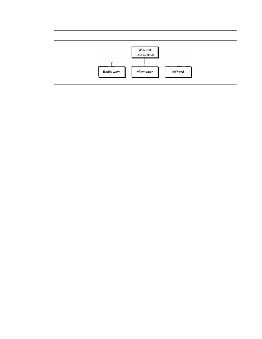
SECTION 7.2
UNGUIDED MEDIA: WIRELESS
205
Figure 7.19
Wireless transmission waves
Radio Waves
Although there is no clear-cut demarcation between radio waves and microwaves, elec-
tromagnetic waves ranging in frequencies between 3 kHz and 1 GHz are normally called
radio waves; waves ranging in frequencies between 1 and 300 GHz are called micro-
waves. However, the behavior of the waves, rather than the frequencies, is a better
criterion for classification.
Radio waves, for the most part, are omnidirectional. When an antenna transmits
radio waves, they are propagated in all directions. This means that the sending and
receiving antennas do not have to be aligned. A sending antenna sends waves that can
be received by any receiving antenna. The omnidirectional property has a disadvantage,
too. The radio waves transmitted by one antenna are susceptible to interference by
another antenna that may send signals using the same frequency or band.
Radio waves, particularly those waves that propagate in the sky mode, can travel
long distances. This makes radio waves a good candidate for long-distance broadcast-
ing such as AM radio.
Radio waves, particularly those of low and medium frequencies, can penetrate walls.
This characteristic can be both an advantage and a disadvantage.
It
is an advantage
because, for example, an AM radio can receive signals inside a building.
It
is a disadvan-
tage because we cannot isolate a communication to just inside or outside a building. The
radio wave band is relatively narrow, just under 1 GHz, compared to the microwave
band. When this band is divided into subbands, the subbands are also narrow, leading to a
low data rate for digital communications.
Almost the entire band is regulated by authorities (e.g., the FCC in the United
States). Using any part of the band requires permission from the authorities.
Omnidirectional Antenna
Radio waves use omnidirectional antennas that send out signals in all directions.
Based on the wavelength, strength, and the purpose of transmission, we can have sev-
eral types of antennas. Figure 7.20 shows an omnidirectional antenna.
Applications
The omnidirectional characteristics of radio waves make them useful for multicasting,
in which there is one sender but many receivers. AM and FM radio, television, mari-
time radio, cordless phones, and paging are examples of multicasting.
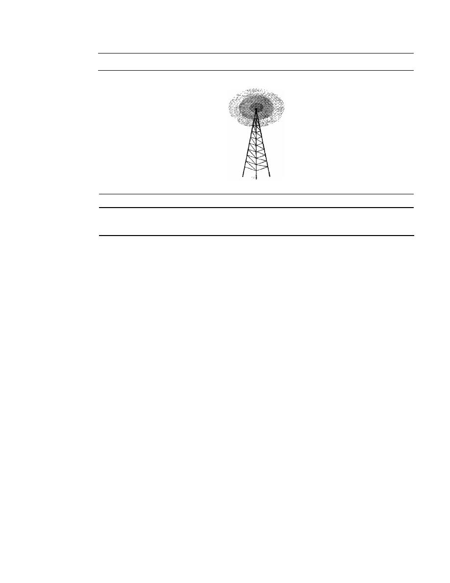
206
CHAPTER
7
TRANSMISSION MEDIA
Figure 7.20
Omnidirectional antenna
Radio waves are used for multicast communications,
such as radio and television, and paging systems.
Microwaves
Electromagnetic waves having frequencies between I and 300 GHz are called micro-
waves.
Microwaves are unidirectional. When an antenna transmits microwave waves, they
can be narrowly focused. This means that the sending and receiving antennas need to
be aligned. The unidirectional property has an obvious advantage. A pair of antennas
can be aligned without interfering with another pair of aligned antennas. The following
describes some characteristics of microwave propagation:
o
Microwave propagation is line-of-sight. Since the towers with the mounted antennas
need to be in direct sight of each other, towers that are far apart need to be very tall.
The curvature of the earth as well as other blocking obstacles do not allow two short
towers to communicate by using microwaves. Repeaters are often needed for long-
distance communication.
o
Very high-frequency microwaves cannot penetrate walls. This characteristic can be
a disadvantage if receivers are inside buildings.
o
The microwave band is relatively wide, almost 299 GHz. Therefore wider subbands
can be assigned, and a high data rate is possible
o
Use of certain portions of the band requires permission from authorities.
Unidirectional Antenna
Microwaves need
unidirectional antennas
that send out signals in one direction. Two
types of antennas are used for microwave communications: the parabolic dish and the
hom (see Figure 7.21).
A parabolic dish antenna
is based on the geometry of a parabola: Every line
parallel to the line of symmetry (line of sight) reflects off the curve at angles such that
all the lines intersect in a common point called the focus. The parabolic dish works as a
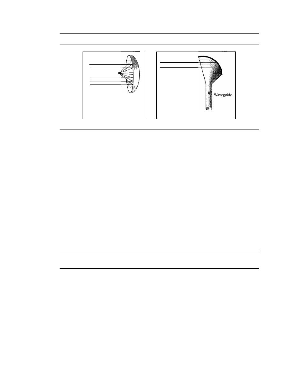
SECTION 7.2
UNGUIDED MEDIA: WIRELESS
207
Figure 7.21
Unidirectional antennas
Focus
a. Dish antenna
b. Horn antenna
funnel, catching a wide range of waves and directing them to a common point. In
this way, more of the signal is recovered than would be possible with a single-point
receiver.
Outgoing transmissions are broadcast through a horn aimed at the dish. The micro-
waves hit the dish and are deflected outward in a reversal of the receipt path.
A
horn antenna
looks like a gigantic scoop. Outgoing transmissions are broadcast
up a stem (resembling a handle) and deflected outward in a series of narrow parallel
beams by the curved head. Received transmissions are collected by the scooped shape of
the horn, in a manner similar to the parabolic dish, and are deflected down into the stem.
Applications
Microwaves, due to their unidirectional properties, are very useful when unicast
(one-to-one) communication is needed between the sender and the receiver. They are
used in cellular phones (Chapter 16), satellite networks (Chapter 16), and wireless LANs
(Chapter 14).
Microwaves are used for unicast communication such as cellular telephones,
satellite networks, and wireless LANs.
Infrared
Infrared waves,
with frequencies from
300
GHz to
400
THz (wavelengths from 1 mm
to 770 nm), can be used for short-range communication. Infrared waves, having high
frequencies, cannot penetrate walls. This advantageous characteristic prevents interfer-
ence between one system and another; a short-range communication system in one room
cannot be affected by another system in the next room. When we use our infrared remote
control, we do not interfere with the use of the remote by our neighbors. However, this
same characteristic makes infrared signals useless for long-range communication. In
addition, we cannot use infrared waves outside a building because the sun's rays contain
infrared waves that can interfere with the communication.

208
CHAPTER
7
TRANSMISSION MEDIA
Applications
The infrared band, almost 400 THz, has an excellent potential for data transmission.
Such a wide bandwidth can be used to transmit digital data with a very high data rate.
The
Infrared Data Association (IrDA), an association for sponsoring the use of infrared
waves, has established standards for using these signals for communication between
devices such as keyboards, mice, PCs, and printers. For example, some manufacturers
provide a special port called the IrDA port that allows a wireless keyboard to commu-
nicate with a PC. The standard originally defined a data rate of
75 kbps for a distance
up to
8
m. The recent standard defines a data rate of 4 Mbps.
Infrared signals defined by IrDA transmit through line of sight; the IrDA port on
the keyboard needs to point to the PC for transmission to occur.
Infrared signals can be used for short-range communication
in a closed area using line-of-sight propagation.
7.3
RECOMMENDED READING
For more details about subjects discussed in this chapter, we recommend the following
books. The items in brackets [...] refer to the reference list at the end of the text.
Books
Transmission media is discussed in Section 3.8 of [GW04], Chapter 4 of [Sta04], Sec-
tion
2.2
and 2.3 of [Tan03]. [SSS05] gives a full coverage of transmission media.
7.4
KEY TERMS
angle of incidence
Bayone-Neil-Concelman (BNC)
connector
cladding
coaxial cable
core
critical angle
electromagnetic spectrum
fiber-optic cable
gauge
ground propagation
guided media
horn antenna
infrared wave
IrDA port
line-of-sight propagation
microwave
MT-RJ
multimode graded-index fiber
multimode step-index fiber
omnidirectional antenna
optical fiber
parabolic dish antenna
Radio Government (RG) number
radio wave
reflection
refraction
RJ45

shielded twisted-pair (STP)
single-mode fiber
sky propagation
straight-tip (ST) connector
subscriber channel (SC) connector
transmission medium
SECTION
7.6
PRACTICE SET
209
twisted-pair cable
unguided medium
unidirectional antenna
unshielded twisted-pair
(UTP)
wireless communication
7.5
SUMMARY
o
Transmission media lie below the physical layer.
D
A guided medium provides a physical conduit from one device to another. Twisted-
pair cable, coaxial cable, and optical fiber are the most popular types of guided
media.
D
Twisted-pair cable consists of two insulated copper wires twisted together. Twisted-
pair cable is used for voice and data communications.
D
Coaxial cable consists of a central conductor and a shield. Coaxial cable can carry
signals of higher frequency ranges than twisted-pair cable. Coaxial cable is used in
cable TV networks and traditional Ethernet LANs.
o
Fiber-optic cables are composed of a glass or plastic inner core surrounded by
cladding, all encased in an outside jacket. Fiber-optic cables carry data signals in
the form of light. The signal is propagated along the inner core by reflection. Fiber-
optic transmission is becoming increasingly popular due to its noise resistance, low
attenuation, and high-bandwidth capabilities. Fiber-optic cable is used in backbone
networks, cable TV networks, and Fast Ethernet networks.
D
Unguided media (free space) transport electromagnetic waves without the use of a
physical conductor.
o
Wireless data are transmitted through ground propagation, sky propagation, and line-
of-sight propagation.Wireless waves can be classified as radio waves, microwaves, or
infrared waves. Radio waves are omnidirectional; microwaves are unidirectional.
Microwaves are used for cellular phone, satellite, and wireless LAN communications.
D
Infrared waves are used for short-range communications such as those between a
PC and a peripheral device.
It
can also be used for indoor LANs.
7.6
PRACTICE SET
Review Questions
1. What is the position of the transmission media in the OSI or the Internet model?
2. Name the two major categories of transmission media.
3. How do guided media differ from unguided media?
4. What are the three major classes of guided media?
5. What is the significance of the twisting in twisted-pair cable?
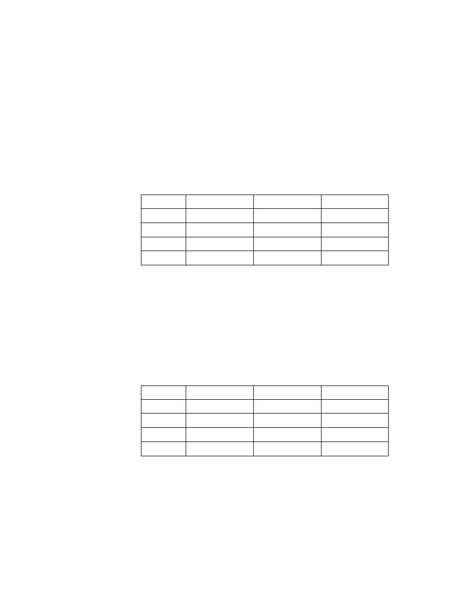
210
CHAPTER
7
TRANSMISSION MEDIA
6. What is refraction? What is reflection?
7. What is the purpose of cladding in an optical fiber?
8. Name the advantages of optical fiber over twisted-pair and coaxial cable.
9. How does sky propagation differ from line-of-sight propagation?
10. What is the difference between omnidirectional waves and unidirectional waves?
Exercises
11. Using Figure 7.6, tabulate the attenuation (in dB) of a 18-gauge UTP for the indicated
frequencies and distances.
Table 7.5
Attenuation/or I8-gauge UTP
Distance
dB at
1
KHz
dRat
10KHz
dB at 100
KHz
1 Krn
lOKm
15 Krn
20Km
12. Use the result of Exercise 11 to infer that the bandwidth of a UTP cable decreases
with an increase in distance.
13.
If
the power at the beginning of a 1
KIn
18-gauge UTP is 200 mw, what is the
power at the end for frequencies 1 KHz, 10 KHz, and 100 KHz? Use the result of
Exercise 11.
14. Using Figure 7.9, tabulate the attenuation (in dB) of a 2.6/9.5 mm coaxial cable for
the indicated frequencies and distances.
Table 7.6
Attenuation/or
2.6/9.5 mm coaxial cable
Distance
dB at
1
KHz
dB at 10 KHz
dB at 100KHz
1 Km
lOKrn
15Km
20Km
15. Use the result of Exercise 14 to infer that the bandwidth of a coaxial cable
decreases with the increase in distance.
16.
If
the power at the beginning of a 1
KIn
2.6/9.5 mm coaxial cable is 200 mw, what
is the power at the end for frequencies 1 KHz, 10KHz, and 100 KHz? Use the
result of Exercise 14.
17. Calculate the bandwidth of the light for the following wavelength ranges (assume a
propagation speed of 2 x 10
8
m):
a. 1000 to 1200 nm
b. 1000 to 1400 nm

SECTION
7.6
PRACTICE SET
211
18. The horizontal axes in Figure 7.6 and 7.9 represent frequencies. The horizontal
axis in Figure 7.16 represents wavelength. Can you explain the reason? lfthe prop-
agation speed
in
an optical fiber is 2 x 10
8
ill, can you change the units in the hori-
zontal axis to frequency? Should the vertical-axis units be changed too? Should the
curve be changed too?
19. Using Figure 7.16, tabulate the attenuation (in dB) of an optical fiber for the indicated
wavelength and distances.
Table 7.7
Attenuation for optical fiber
Distance
dB at 800 nm
dB at 1000 nm
dB at 1200nm
1 Km
lOKm
15Km
20Km
20. A light signal is travelling through a fiber. What is the delay
in
the signal if the
length of the fiber-optic cable is 10 m, 100 m, and 1 Km (assume a propagation
speed of 2 x 10
8
ill)?
21. A beam oflight moves from one medium to another medium with less density. The
critical angle is 60°. Do we have refraction or reflection for each of the following
incident angles? Show the bending of the light ray in each case.
a.
40°
b. 60°
c.
80
0

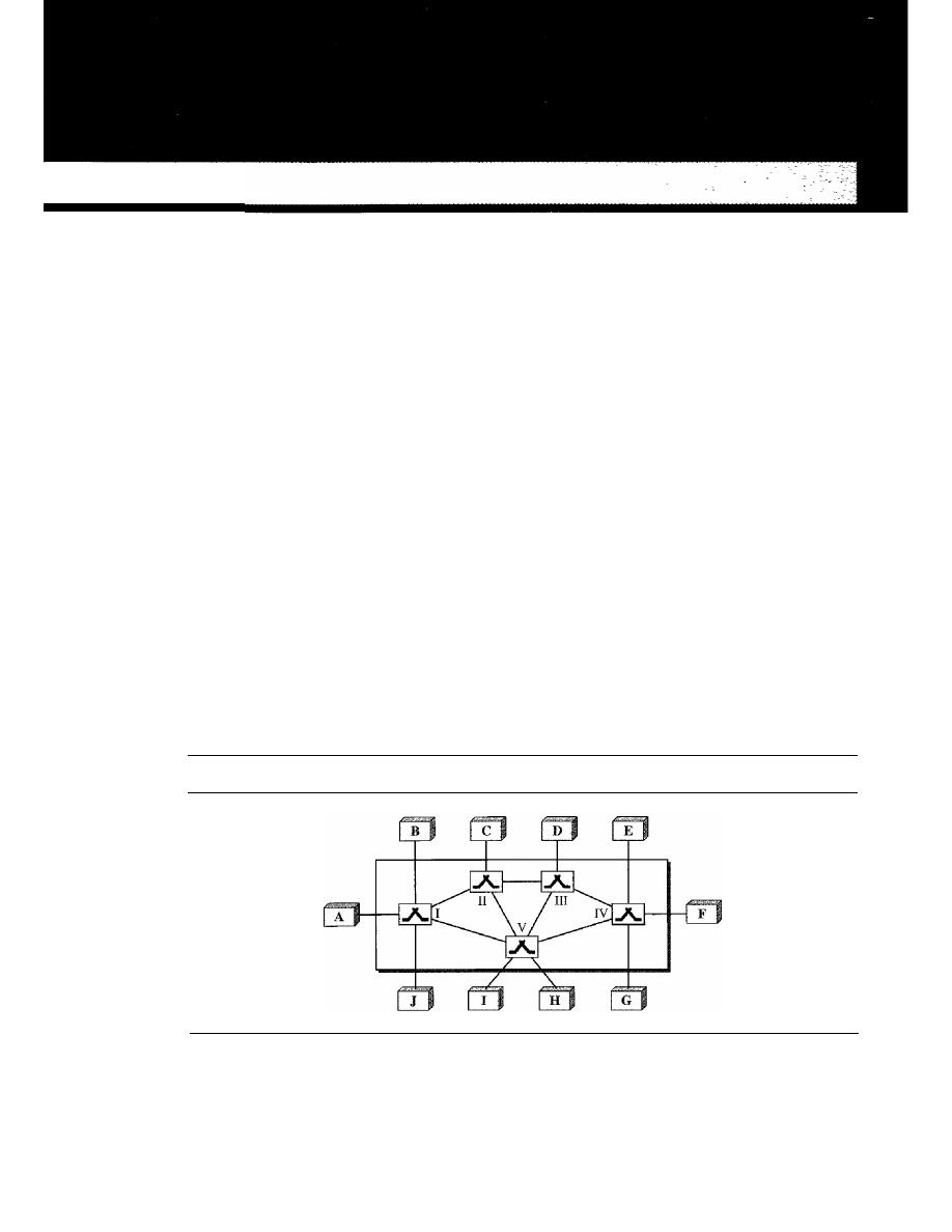
CHAPTER 8
Switching
A network is a set of connected devices. Whenever we have multiple devices, we have
the problem of how to connect them to make one-to-one communication possible. One
solution is to make a point-to-point connection between each pair of devices (a mesh
topology) or between a central device and every other device (a star topology). These
methods, however, are impractical and wasteful when applied to very large networks.
The number and length of the links require too much infrastructure to be cost-efficient,
and the majority of those links would be idle most of the time. Other topologies
employing multipoint connections, such as a bus, are ruled out because the distances
between devices and the total number of devices increase beyond the capacities of the
media and equipment.
A better solution is
switching.
A switched network consists of a series of interlinked
nodes, called
switches.
Switches are devices capable of creating temporary connections
between two or more devices linked
to
the switch. In a switched network, some of these
nodes are connected to the end systems (computers or telephones, for example). Others
are used only for routing. Figure 8.1 shows a switched network.
Figure 8.1
Switched network
The
end systems
(communicating devices) are labeled A, B, C, D, and so on, and the
switches are labeled I, II, III, IV, and V. Each switch is connected to multiple links.
213
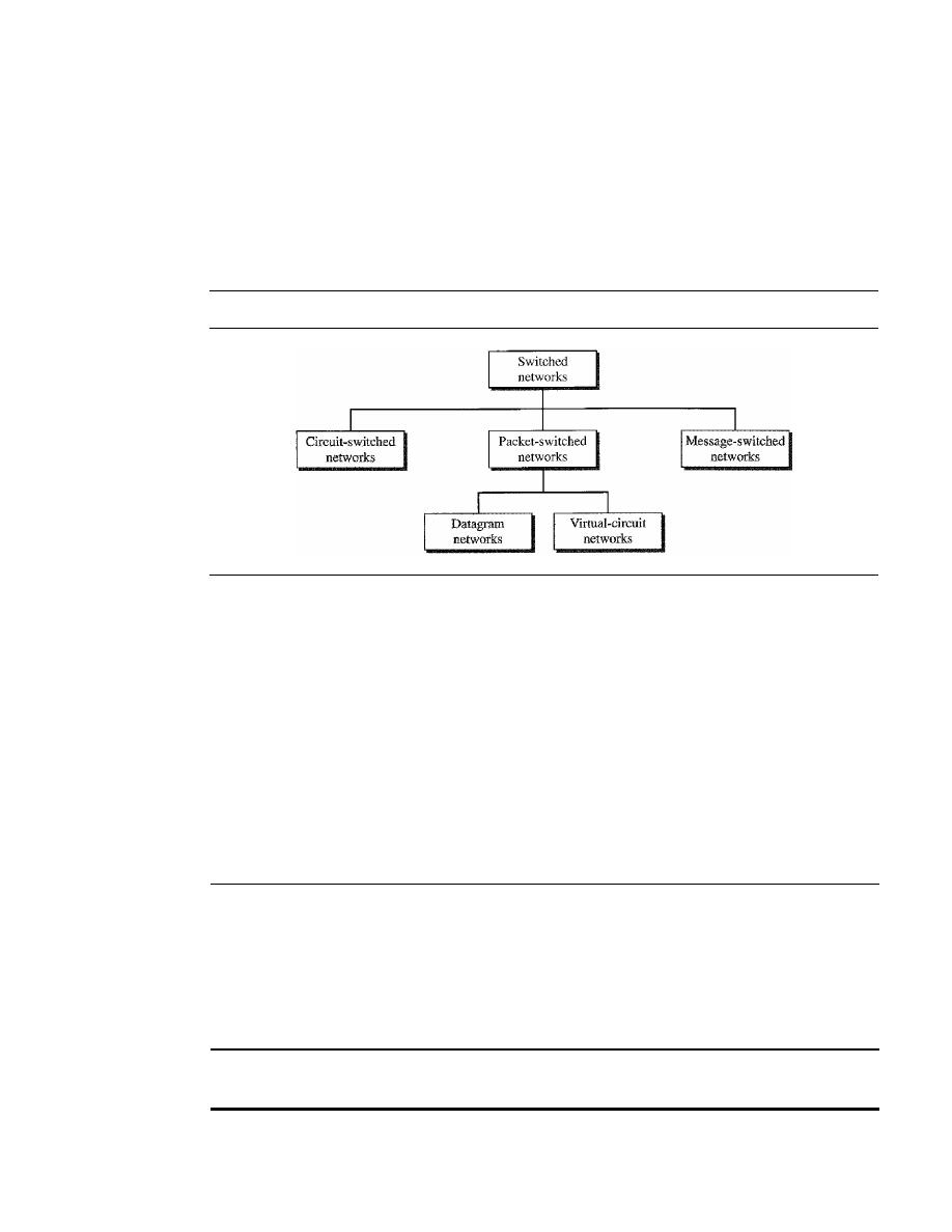
214
CHAPTER
8
SWITCHING
Traditionally, three methods of switching have been important: circuit switching,
packet switching, and message switching. The first two are commonly used today. The
third has been phased out in general communications but still has networking applications.
We can then divide today's networks into three broad categories: circuit-switched networks,
packet-switched networks, and message-switched. Packet-switched networks can funher
be divided into two subcategories-virtual-circuit networks and datagram networks-
as shown in Figure 8.2.
Figure 8.2
Taxonomy of switched networks
We can say that the virtual-circuit networks have some common characteristics
with circuit-switched and datagram networks. Thus, we first discuss circuit-switched
networks, then datagram networks, and finally virtual-circuit networks.
Today the tendency in packet switching is to combine datagram networks and virtual-
circuit networks. Networks route the first packet based on the datagram addressing idea,
but then create a virtual-circuit network for the rest of the packets coming from the same
source and going to the same destination. We will see some of these networks in future
chapters.
In message switching, each switch stores the whole message and forwards it to the
next switch. Although, we don't see message switching at lower layers, it is still used in
some applications like electronic mail (e-mail). We will not discuss this topic in this book.
8.1
CIRCUIT-SWITCHED NETWORKS
A
circuit-switched network
consists of a set of switches connected by physical links.
A connection between two stations is a dedicated path made of one or more links. How-
ever, each connection uses only one dedicated channel on each link. Each link is nor-
mally divided into n channels by using FDM or TDM as discussed in Chapter 6.
A circuit-switched network is made of a set of switches connected by physical links,
in which each link is divided into
n
channels.
Figure 8.3 shows a trivial circuit-switched network with four switches and four
links. Each link is divided into
n (n
is 3 in the figure) channels by using FDM or TDM.
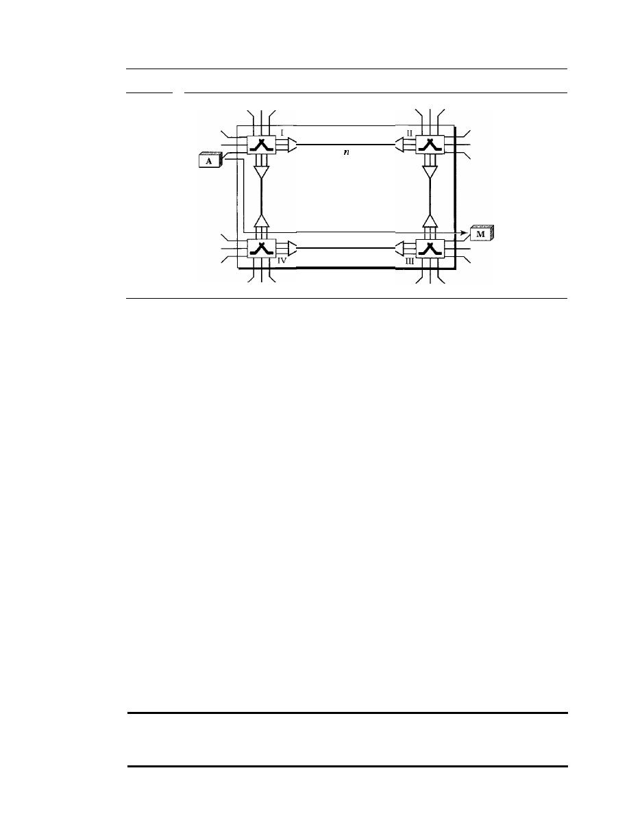
SECTION
8.1
CIRCUIT-SWITCHED NETWORKS
215
Figure 8.3
A trivial circuit-switched network
One link,
channels
Path
We have explicitly shown the multiplexing symbols to emphasize the division of the
link into channels even though multiplexing can be implicitly included in the switch
fabric.
The end systems, such as computers or telephones, are directly connected to a
switch. We have shown only two end systems for simplicity. When end system A needs
to communicate with end system M, system A needs to request a connection to M that
must be accepted by all switches as well as by M itself. This is called the setup phase;
a circuit (channel) is reserved on each link, and the combination of circuits or channels
defines the dedicated path. After the dedicated path made of connected circuits (channels)
is established, data transfer can take place. After all data have been transferred, the
circuits are tom down.
We need to emphasize several points here:
D
Circuit switching takes place at the physical layer.
D
Before starting communication, the stations must make a reservation for the resources
to be used during the communication. These resources, such as channels (bandwidth
in FDM and time slots in TDM), switch buffers, switch processing time, and switch
input/output ports, must remain dedicated during the entire duration of data transfer
until the teardown phase.
D
Data transferred between the two stations are not packetized (physical layer transfer
of the signal). The data are a continuous flow sent by the source station and received
by the destination station, although there may be periods of silence.
D
There is no addressing involved during data transfer. The switches route the data
based on their occupied band (FDM) or time slot (TDM). Of course, there is end-to-
end addressing used during the setup phase, as we will see shortly.
In circuit switching, the resources need to be reserved during the setup phase;
the resources remain dedicated for the entire duration
of data transfer until the teardown phase.
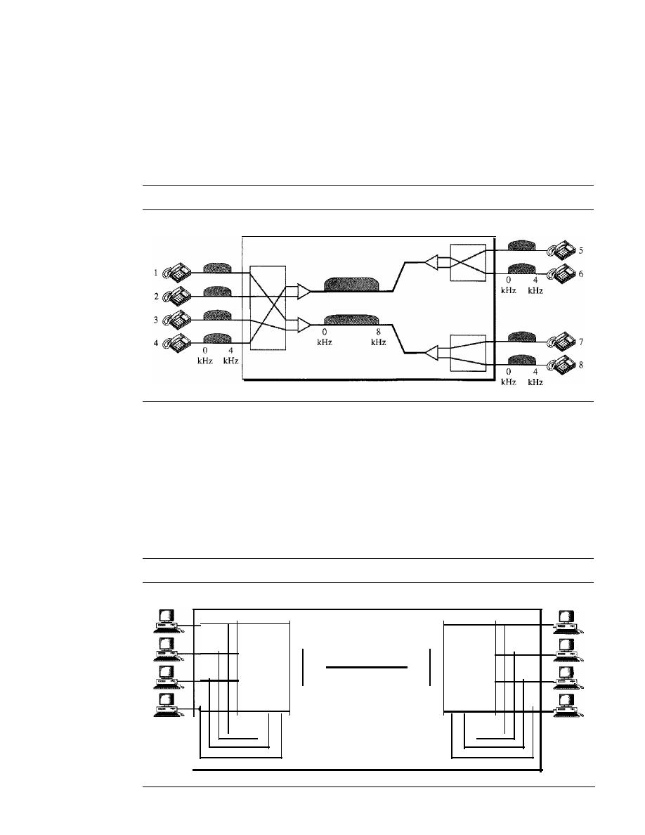
216
CHAPTER
8
SWITCHING
Example 8.1
As a trivial example, let us use a circuit-switched network to connect eight telephones in a small
area. Communication is through 4-kHz voice channels. We assume that each link uses FDM to
connect a maximum of two voice channels. The bandwidth of each link is then 8 kHz. Figure 8.4
shows the situation. Telephone 1 is connected to telephone 7; 2 to
5;
3 to 8; and 4 to 6. Of course
the situation may change when new connections are made. The switch controls the connections.
Figure 8.4
Circuit-switched network used in Example 8.1
Circuit-switched network
Example 8.2
As another example, consider a circuit-switched network that connects computers in two remote
offices of a private company. The offices are connected using a T-l line leased from a communi-
cation service provider. There are two 4
X
8 (4 inputs and 8 outputs) switches in this network. For
each switch, four output ports are folded into the input ports to allow communication between
computers in the same office. Four other output ports allow communication between the two
offices. Figure 8.5 shows the situation.
Figure 8.5
Circuit-switched network used
in
Example 8.2
Circuit-switched network
4x8
swItch
T-l line with
1.544 Mbps
4x8
switch

SECTION
8.1
CIRCUIT-SWITCHED NEIWORKS
217
Three Phases
The actual communication in a circuit-switched network requires three phases: connec-
tion setup, data transfer, and connection teardown.
Setup Phase
Before the two parties (or multiple parties in a conference call) can communicate, a
dedicated circuit (combination of channels in links) needs to be established. The end sys-
tems are normally connected through dedicated lines to the switches, so connection setup
means creating dedicated channels between the switches. For example, in Figure 8.3,
when system A needs to connect to system M, it sends a setup request that includes the
address of system M, to switch I. Switch I finds a channel between itself and switch IV
that can be dedicated for this purpose. Switch I then sends the request to switch IV,
which finds a dedicated channel between itself and switch III. Switch III informs sys-
tem M of system A's intention at this time.
In the next step to making a connection, an acknowledgment from system M needs
to be sent in the opposite direction to system A. Only after system A receives this
acknowledgment is the connection established.
Note that end-to-end addressing is required for creating a connection between the
two end systems. These can be, for example, the addresses of the computers assigned
by the administrator in a TDM network, or telephone numbers in an FDM network.
Data Transfer Phase
After the establishment of the dedicated circuit (channels), the two parties can transfer data.
Teardown Phase
When one of the parties needs to disconnect, a signal is sent to each switch to release
the resources.
Efficiency
It
can be argued that circuit-switched networks are not as efficient as the other two
types of networks because resources are allocated during the entire duration of the con-
nection. These resources are unavailable to other connections. In a telephone network,
people normally terminate the communication when they have finished their conversation.
However, in computer networks, a computer can be connected to another computer
even if there is no activity for a long time. In this case, allowing resources to be dedicated
means that other connections are deprived.
Delay
Although a circuit-switched network normally has low efficiency, the delay in this type
of network is minimal. During data transfer the data are not delayed at each switch; the
resources are allocated for the duration of the connection. Figure 8.6 shows the idea of
delay in a circuit-switched network when only two switches are involved.
As Figure 8.6 shows, there is no waiting time at each switch. The total delay is due
to the time needed to create the connection, transfer data, and disconnect the circuit. The
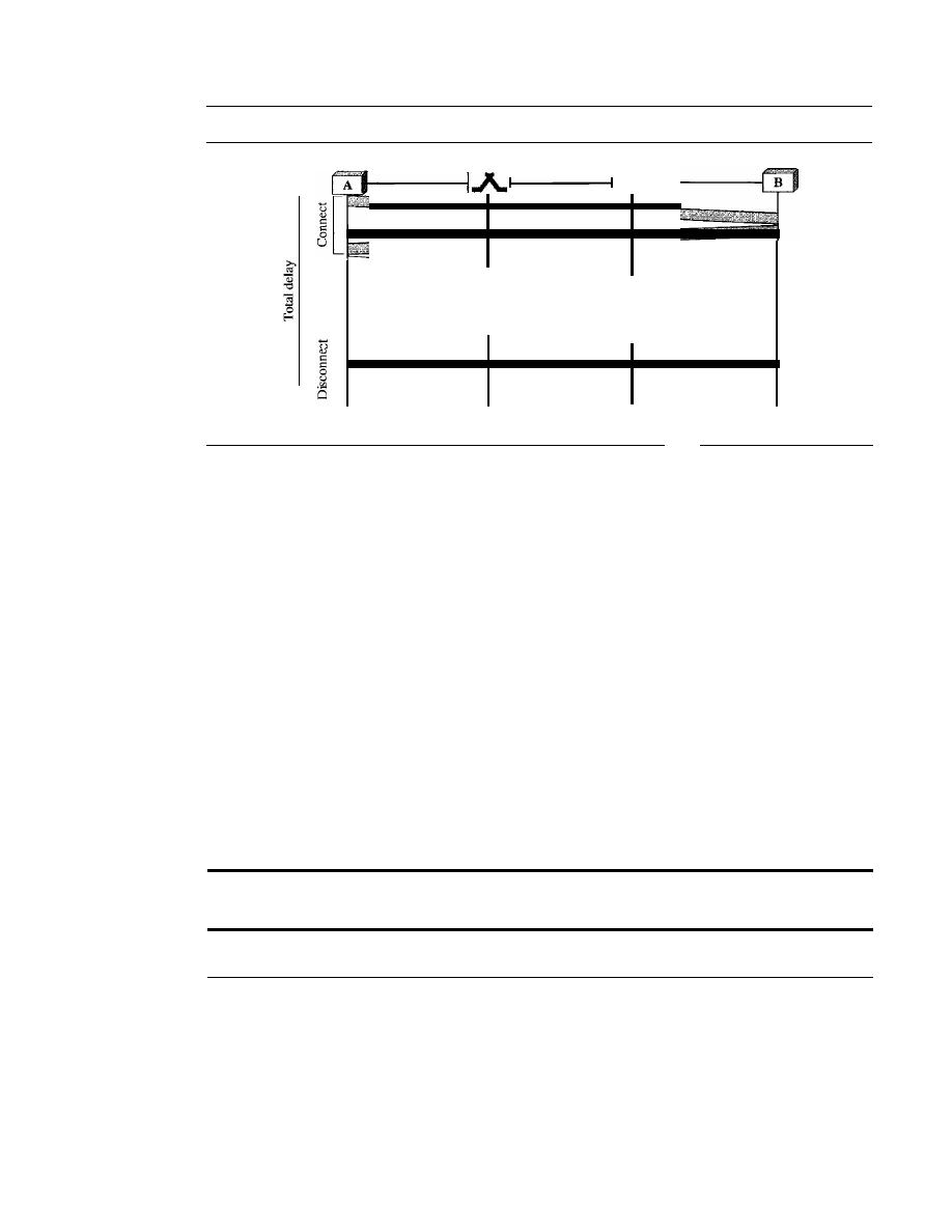
218
CHAPTER
8
SWITCHING
Figure 8.6
Delay in a circuit-switched network
Data transfer
[------------------
Time
Time
Time
Time
delay caused by the setup is the sum of four parts: the propagation time of the source
computer request (slope of the first gray box), the request signal transfer time (height of
the first gray box), the propagation time of the acknowledgment from the destination
computer (slope of the second gray box), and the signal transfer time of the acknowledg-
ment (height of the second gray box). The delay due to data transfer is the sum of two
parts: the propagation time (slope of the colored box) and data transfer time (height of
the colored box), which can be very long. The third box shows the time needed to tear
down the circuit. We have shown the case in which the receiver requests disconnection,
which creates the maximum delay.
Circuit-Switched Technology in Telephone Networks
As we will see in Chapter 9, the telephone companies have previously chosen the circuit-
switched approach to switching in the physical layer; today the tendency is moving
toward other switching techniques. For example, the telephone number is used as the
global address, and a signaling system (called SS7) is used for the setup and teardown
phases.
Switching at the
physical layer in the traditional telephone
network
uses
the circuit-switching approach.
8.2
DATAGRAM NETWORKS
In data communications, we need to send messages from one end system to another.
If
the message is going to pass through a packet-switched network, it needs to be divided
into packets of fixed or variable size. The size of the packet is determined by the net-
work and the governing protocol.
In packet switching, there is no resource allocation for a packet. This means that
there is no reserved bandwidth on the links, and there is no scheduled processing time
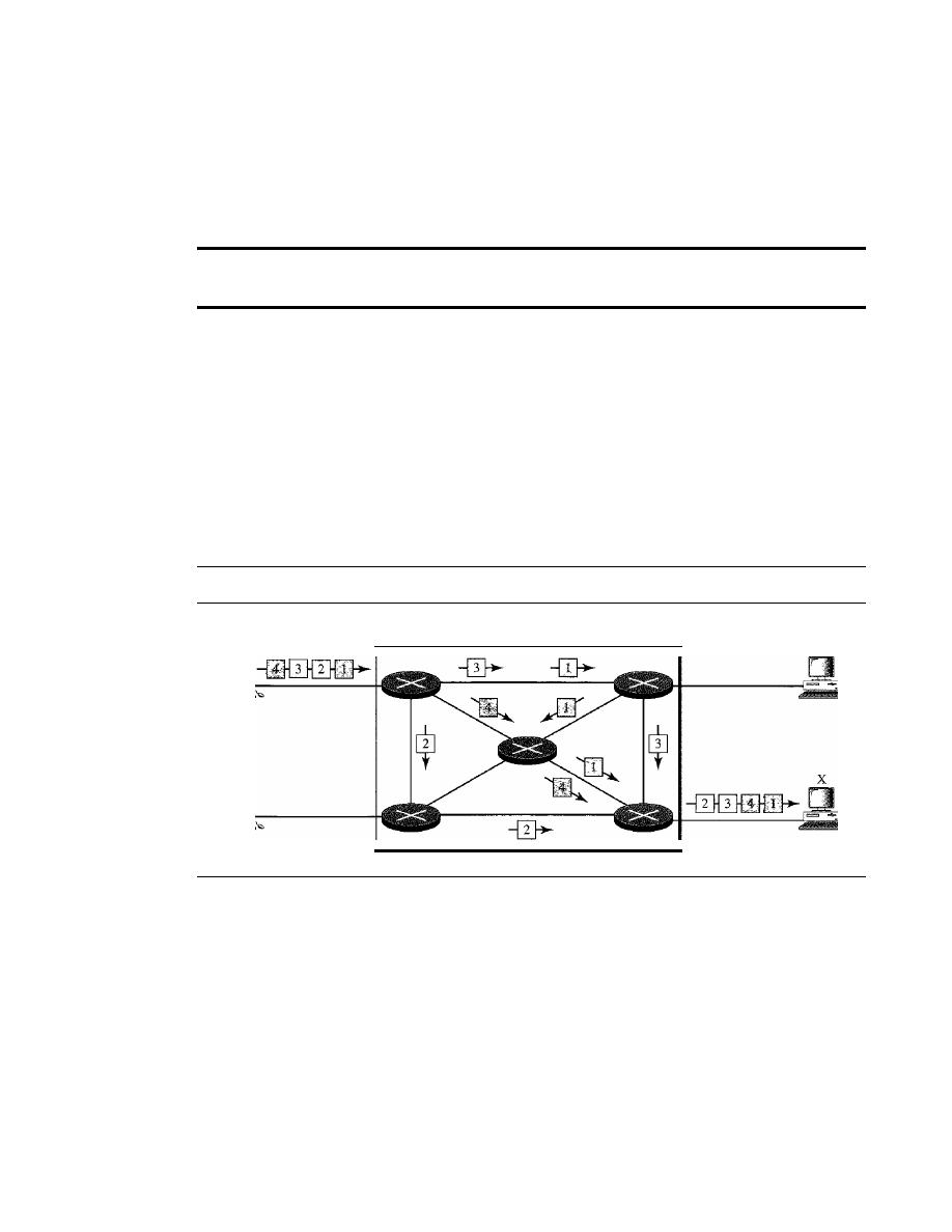
SECTION
8.2
DATAGRAM NETWORKS
219
for each packet. Resources are allocated on demand. The allocation is done on a first-
come, first-served basis. When a switch receives a packet, no matter what is the source
or destination, the packet must wait if there are other packets being processed. As with
other systems in our daily life, this lack of reservation may create delay. For example, if
we do not have a reservation at a restaurant, we might have to wait.
In a packet-switched network, there is no resource reservation;
resources are allocated on demand.
In a
datagram network,
each packet is treated independently of all others. Even if
a packet is part of a multipacket transmission, the network treats it as though it existed
alone. Packets in this approach are referred to as
datagrams.
Datagram switching is normally done at the network layer. We briefly discuss
datagram networks here as a comparison with circuit-switched and virtual-circuit-
switched networks. In Part 4 of this text, we go into greater detail.
Figure 8.7 shows how the datagram approach is used to deliver four packets from
station A to station X. The switches in a datagram network are traditionally referred to
as routers. That is why we use a different symbol for the switches in the figure.
Figure 8.7
A datagram network with four switches (routers)
Datagram network
A
In this example, all four packets (or datagrams) belong to the same message, but
may travel different paths to reach their destination. This is so because the links may be
involved in carrying packets from other sources and do not have the necessary bandwidth
available to carry all the packets from A to X. This approach can cause the datagrams of
a transmission to arrive at their destination out of order with different delays between the
packets. Packets may also be lost or dropped because of a lack of resources. In most
protocols, it is the responsibility of an upper-layer protocol to reorder the datagrams or
ask for lost datagrams before passing them on to the application.
The datagram networks are sometimes referred to as
connectionless networks.
The
term connectionless here means that the switch (packet switch) does not keep information
about the connection state. There are no setup or teardown phases. Each packet is treated
the same by a switch regardless of its source or destination.
220
CHAPTER
8
SWITCHING
Routing Table
If there are no setup or teardown phases, how are the packets routed to their destinations
in a datagram network? In this type of network, each switch (or packet switch) has a rout-
ing table which is based on the destination address. The routing tables are dynamic and
are updated periodically. The destination addresses and the corresponding forwarding
output ports are recorded in the tables. This is different from the table of a circuit-
switched network in which each entry is created when the setup phase is completed and
deleted when the teardown phase is over. Figure 8.8 shows the routing table for a
switch.
Figure 8.8
Routing table in a datagram network
Destination
Output
address
port
1232
I
4150
2
.
.
9130
3
-
-
1
4
21
3
A switch
in
a
datagram
network uses a routing table that
is
based on the destination address.
Destination Address
Every packet in a datagram network carries a header that contains, among other infor-
mation, the destination address of the packet. When the switch receives the packet, this
destination address is examined; the routing table is consulted to find the corresponding
port through which the packet should be forwarded. This address, unlike the address
in a virtual-circuit-switched network, remains the same during the entire journey of the
packet.
The destination address in the header of a packet in a datagram network
remains the same during the entire journey of the packet.
Efficiency
The efficiency of a datagram network is better than that of a circuit-switched network;
resources are allocated only when there are packets to be transferred. If a source sends
a packet and there is a delay of a few minutes before another packet can be sent, the
resources can be reallocated during these minutes for other packets from other sources.
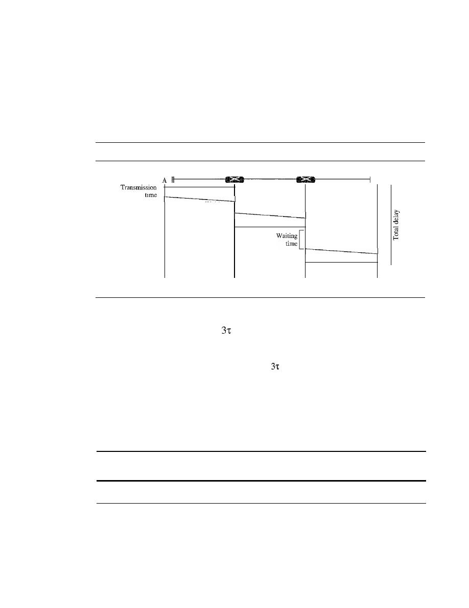
SECTION
8.3
VIRTUAL-CIRCUIT NETWORKS
221
Delay
There may be greater delay in a datagram network than in a virtual-circuit network.
Although there are no setup and teardown phases, each packet may experience a wait at a
switch before it is forwarded. In addition, since not all packets in a message necessarily
travel through the same switches, the delay is not uniform for the packets of a message.
Figure 8.9 gives an example of delay in a datagram network for one single packet.
Figure 8.9
Delay in a datagram network
time
[
Waiting [
time
B
Time
Time
Time
Time
The packet travels through two switches. There are three transmission times
(3T),
three propagation delays (slopes
of the lines), and two waiting times
(WI
+
w2)'
We
ignore the processing time in each switch. The total delay is
Total delay
=
3T
+
+
WI
+
W2
Datagram Networks in the Internet
As we will see in future chapters, the Internet has chosen the datagram approach to
switching at the network layer.
It
uses the universal addresses defined in the network
layer to route packets from the source to the destination.
Switching in the Internet is done by using the datagram
approach to packet switching at the network layer.
8.3
VIRTUAL-CIRCUIT NETWORKS
A virtual-circuit network is a cross between a circuit-switched network and a datagram
network.
It
has some characteristics of both.
1. As in a circuit-switched network, there are setup and teardown phases in addition
to the data transfer phase.
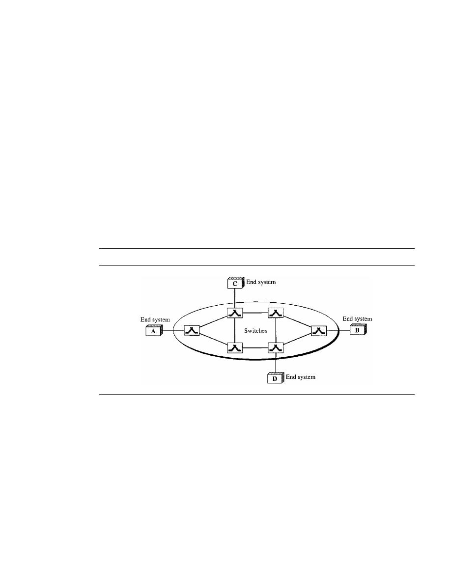
222
CHAPTER
8
SWITCHING
2. Resources can be allocated during the setup phase, as in a circuit-switched network,
or on demand, as in a datagram network.
3. As in a datagram network, data are packetized and each packet carries an address in
the header. However, the address in the header has local jurisdiction (it defines what
should be the next switch and the channel on which the packet is being canied), not
end-to-end jurisdiction. The reader may ask how the intermediate switches know
where to send the packet if there is no final destination address carried by a packet.
The answer will be clear when we discuss virtual-circuit identifiers in the next section.
4. As in a circuit-switched network, all packets follow the same path established during
the connection.
5. A virtual-circuit network is normally implemented in the data link layer, while a
circuit-switched network is implemented in the physical layer and a datagram net-
work in the network layer. But this may change in the future.
Figure
8.10
is an example of a virtual-circuit network. The network has switches that
allow traffic from sources to destinations.
A
source or destination can be a computer,
packet switch, bridge, or any other device that connects other networks.
Figure 8.10
Virtual-circuit network
Addressing
In a virtual-circuit network, two types of addressing are involved: global and local
(virtual-circuit identifier).
Global Addressing
A source or a destination needs to have a global address-an address that can be unique
in the scope of the network or internationally if the network is part of an international
network. However, we will see that a global address in virtual-circuit networks is used
only to create a virtual-circuit identifier, as discussed next.
Virtual-Circuit Identifier
The identifier that is actually used for data transfer is called the virtual-circuit identifier
(Vel).
A
vel,
unlike a global address, is a small number that has only switch scope; it
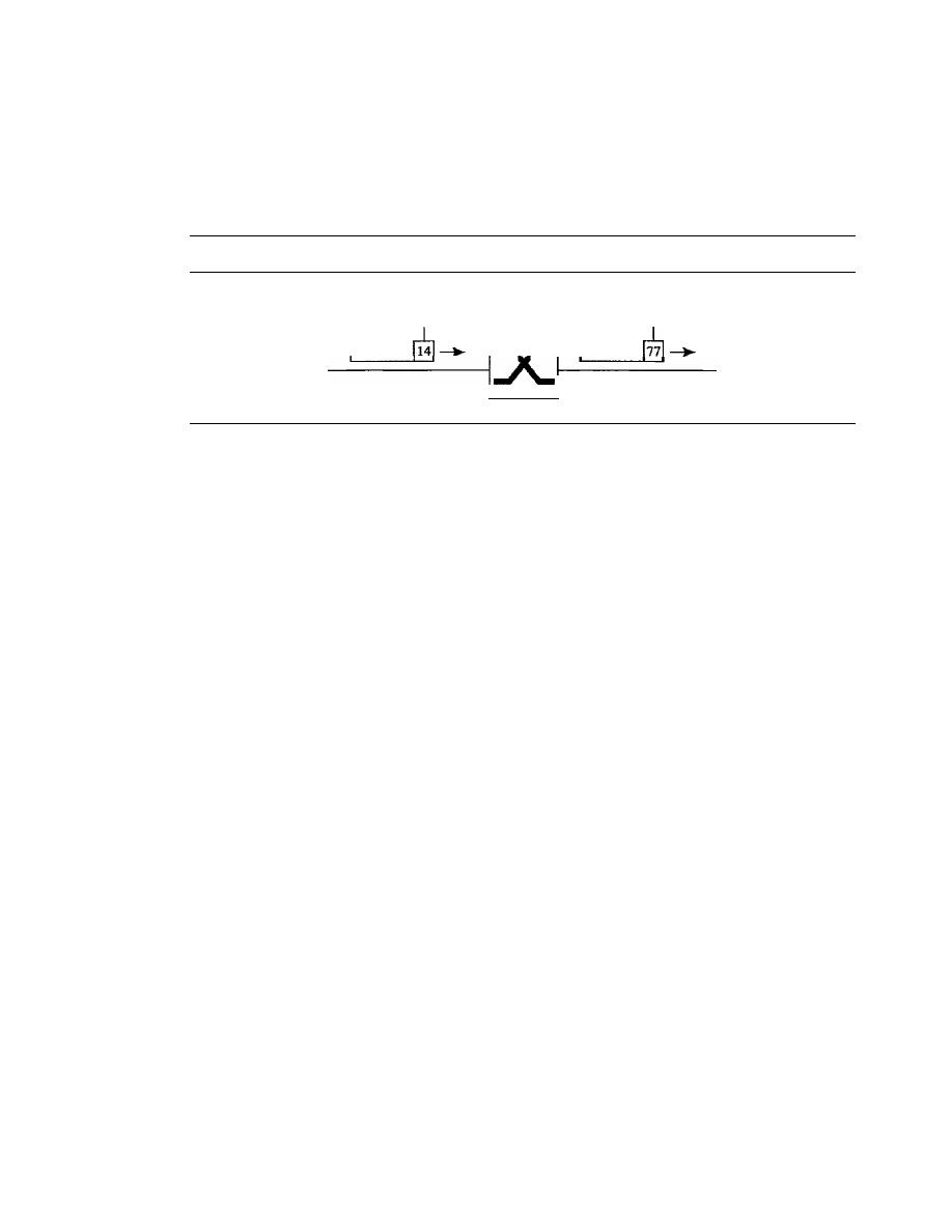
SECTION
8.3
VIRTUAL-CIRCUIT NETWORKS
223
is used by a frame between two switches. When a frame arrives at a switch, it has a
VCI; when it leaves, it has a different VCl. Figure 8.11 shows how the VCI in a data
frame changes from one switch to another. Note that a VCI does not need to be a large
number since each switch can use its own unique set of VCls.
Figure 8.11
Virtual-circuit identifier
VCI
I
VCI
I
Data
I
Data
Three
Phases
As in a circuit-switched network, a source and destination need to go through three
phases in a virtual-circuit network: setup, data transfer, and teardown. In the setup
phase, the source and destination use their global addresses to help switches make table
entries for the connection. In the teardown phase, the source and destination inform the
switches to delete the corresponding entry. Data transfer occurs between these two
phases. We first discuss the data transfer phase, which is more straightforward; we then
talk about the setup and teardown phases.
Data Transfer Phase
To transfer a frame from a source to its destination, all switches need to have a table
entry for this virtual circuit. The table, in its simplest form, has four columns. This
means that the switch holds four pieces of information for each virtual circuit that is
already set up. We show later how the switches make their table entries, but for the
moment we assume that each switch has a table with entries for all active virtual cir-
cuits. Figure 8.12 shows such a switch and its corresponding table.
Figure 8.12 shows a frame arriving at port 1 with a VCI of 14. When the frame
arrives, the switch looks in its table to find port 1 and a VCI of 14. When it is found, the
switch knows to change the VCI to 22 and send out the frame from port 3.
Figure 8.13 shows how a frame from source A reaches destination B and how its
VCI changes during the trip. Each switch changes the VCI and routes the frame.
The data transfer phase is active until the source sends all its frames to the destina-
tion. The procedure at the switch is the same for each frame of a message. The process
creates a virtual circuit, not a real circuit, between the source and destination.
Setup Phase
In the setup phase, a switch creates an entry for a virtual circuit. For example, suppose
source A needs to create a virtual circuit to B. Two steps are required: the setup request
and the acknowledgment.
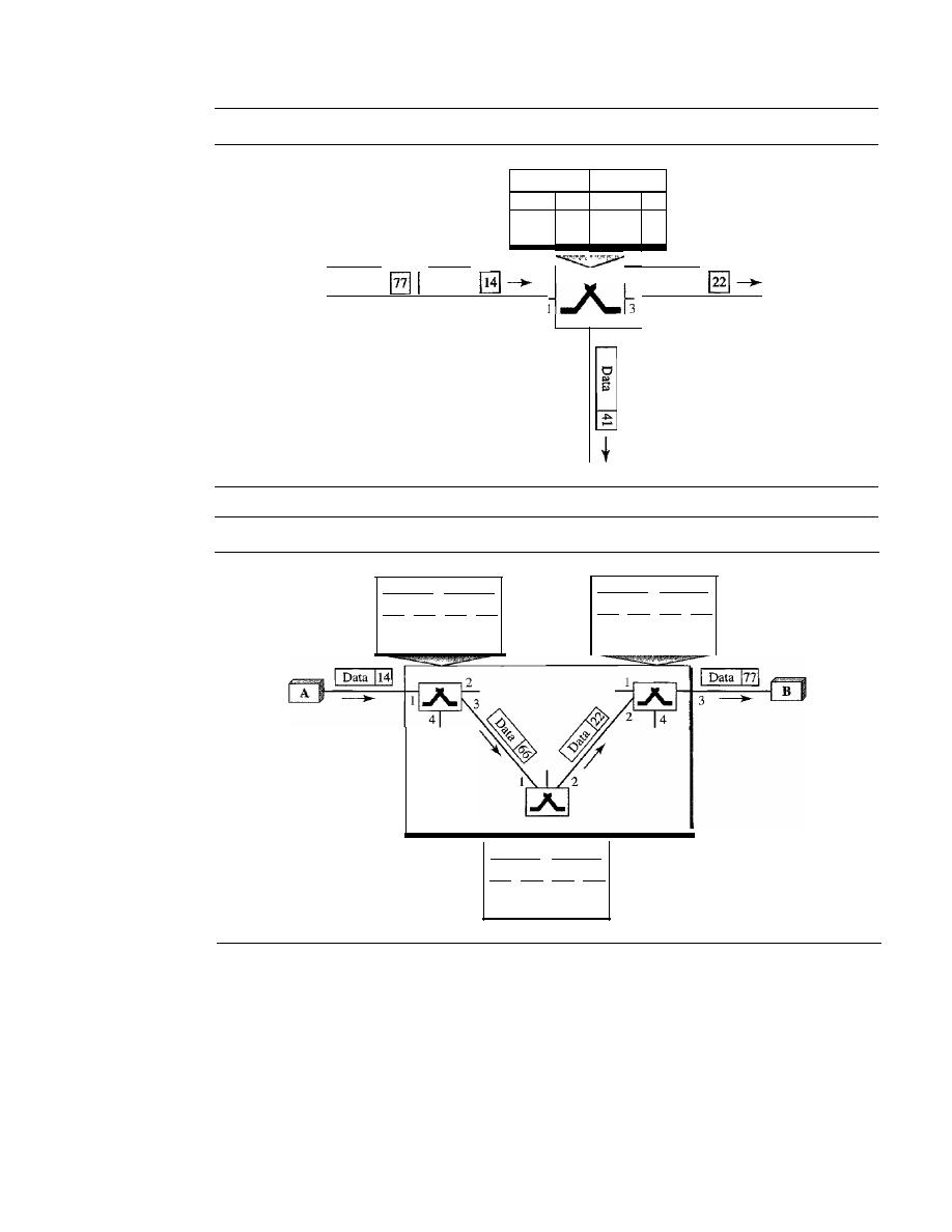
224
CHAPTER
8
SWITCHING
Figure 8.12
Switch and tables in a virtual-circuit network
Incoming
Outgoing
Port
VCl
Port
VCl
1
14
3
22
1
77
2
41
I
Data
Data
I
Data
2
Figure 8.13
Source-to-destination data transfer in a virtual-circuit network
Incoming Outgoing
Port VCl Port VCl
I
14
3
66
Incoming Outgoing
Port VCl Port VCI
2
22
3
77
Incoming Outgoing
Port VCI Port VCl
1
66
2
22
Setup Request
A setup request frame is sent from the source to the destination.
Figure 8.14 shows the process.
a. Source A sends a setup frame to switch 1.
b. Switch 1 receives the setup request frame. It knows that a frame going from A to B
goes out through port 3. How the switch has obtained this information is a point
covered in future chapters. The switch, in the setup phase, acts as a packet switch;
it has a routing table which is different from the switching table. For the moment,
assume that it knows the output port. The switch creates an entry in its table for
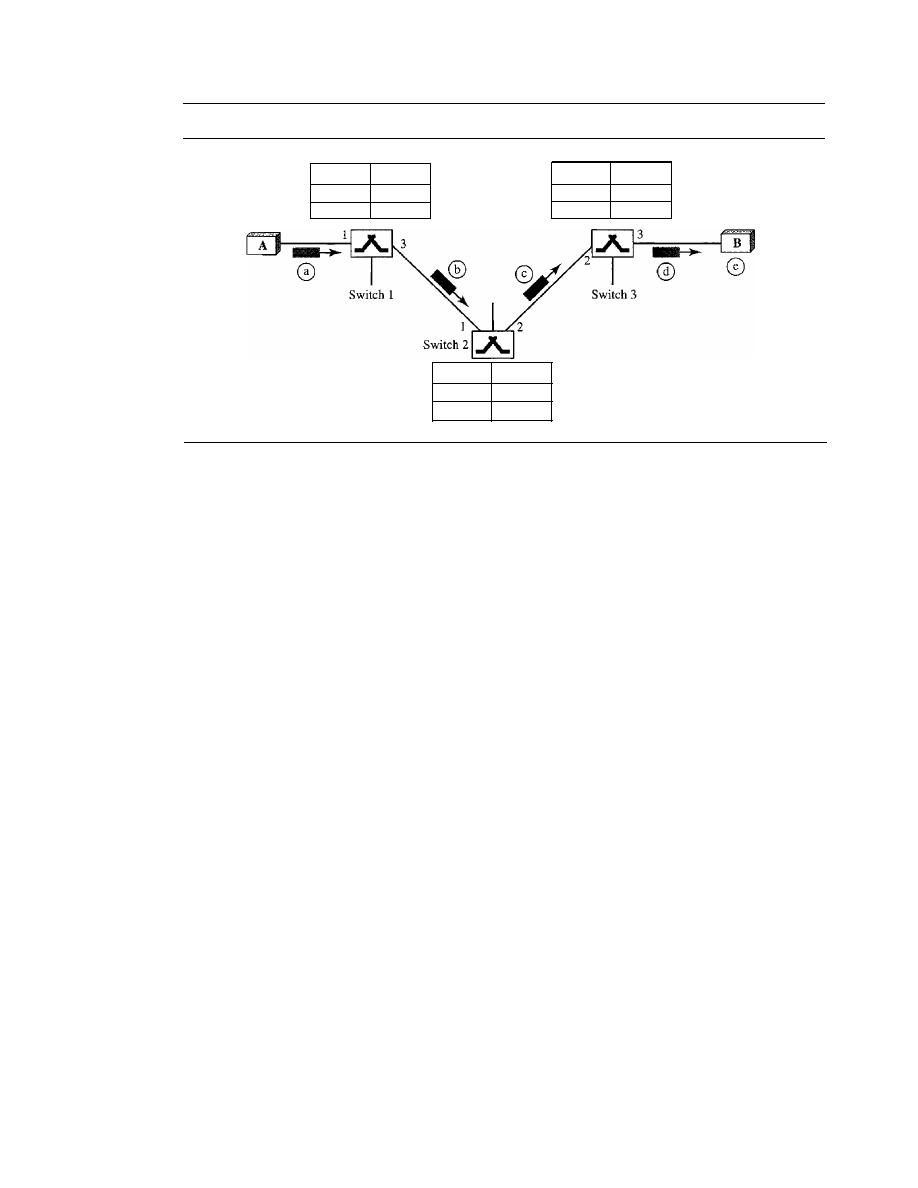
SECTION
8.3
VIRTUAL-CIRCUIT NETWORKS
225
Figure 8.14
Setup request in a virtual-circuit network
Incoming Outgoing
Port IvcI Port IVCI
1
I
14
3
I
Incoming Outgoing
Port IVCI Port IVCI
2
122
3
I
VCI=77
Incoming Outgoing
Port IVCI Port IVCI
I
I 66
2
I
this virtual circuit, but it is only able to fill three of the four columns. The switch
assigns the incoming port
(1)
and chooses an available incoming VCI (14) and the
outgoing port (3). It does not yet know the outgoing VCI, which will be found dur-
ing the acknowledgment step. The switch then forwards the frame through port 3
to switch 2.
c. Switch 2 receives the setup request frame. The same events happen here as at
switch 1; three columns of the table are completed: in this case, incoming port
(l),
incoming VCI (66), and outgoing port (2).
d. Switch 3 receives the setup request frame. Again, three columns are completed:
incoming port (2), incoming VCI (22), and outgoing port (3).
e. Destination B receives the setup frame, and if it is ready to receive frames from A,
it assigns a VCI to the incoming frames that come from A, in this case 77. This
VCI lets the destination know that the frames come from A, and not other sources.
Acknowledgment
A special frame, called the acknowledgment frame, completes
the entries in the switching tables. Figure 8.15 shows the process.
a. The destination sends an acknowledgment to switch 3. The acknowledgment carries
the global source and destination addresses so the switch knows which entry in the
table is to be completed. The frame also carries VCI 77, chosen by the destination as
the incoming VCI for frames from A. Switch 3 uses this VCI to complete the outgoing
VCI column for this entry. Note that 77 is the incoming VCI for destination B, but
the outgoing VCI for switch 3.
b. Switch 3 sends an acknowledgment to switch 2 that contains its incoming VCI in the
table, chosen in the previous step. Switch 2 uses this as the outgoing VCI in the table.
c. Switch 2 sends an acknowledgment to switch 1 that contains its incoming VCI in the
table, chosen in the previous step. Switch 1 uses this as the outgoing VCI in the table.
d. Finally switch 1 sends an acknowledgment to source A that contains its incoming
VCI in the table, chosen in the previous step.
e. The source uses this as the outgoing VCI for the data frames to be sent
to
destination B.
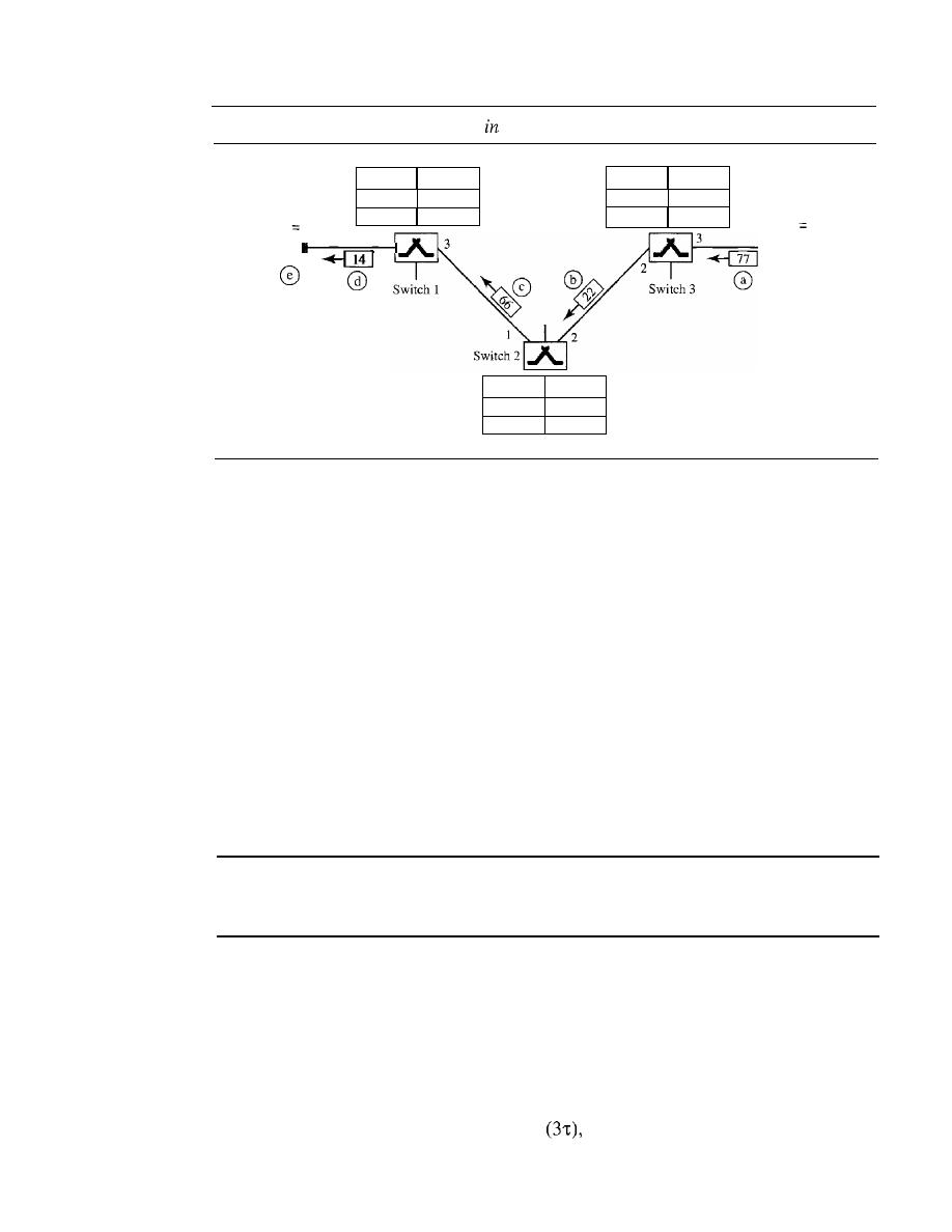
226
CHAPTER
8
SWITCHING
Figure 8.15
Setup acknowledgment
a virtual-circuit network
Incoming Outgoing
Port IVCI Port IVCI
2
122
3
I 77
Incoming Outgoing
Port IVCI Port IVCI
I
I
14
3
166
VCI
14
VCI
77
A
B
Incoming Outgoing
Port IVCI Port IVCI
I
I
66
2
122
Teardowil Phase
In this phase, source A, after sending all frames to B, sends a special frame called a
teardown request.
Destination B responds with a teardown confirmation frame. All
switches delete the corresponding entry from their tables.
Efficiency
As we said before, resource reservation in a virtual-circuit network can be made during
the setup or can be on demand during the data transfer phase. In the first case, the delay
for each packet is the same; in the second case, each packet may encounter different
delays. There is one big advantage in a virtual-circuit network even if resource allocation
is on demand. The source can check the availability of the resources, without actually
reserving it. Consider a family that wants to dine at a restaurant. Although the restaurant
may not accept reservations (allocation of the tables is on demand), the family can call
and find out the waiting time. This can save the family time and effort.
In virtual-circuit switching, all packets belonging to the same source and destination
travel the same path; but the packets may arrive at the destination
with different delays if resource allocation is on demand.
Delay in Virtual-Circuit Networks
In a virtual-circuit network, there is a one-time delay for setup and a one-time delay for
teardown.
If
resources are allocated during the setup phase, there is no wait time for
individual packets. Figure 8.16 shows the delay for a packet traveling through two
switches in a virtual-circuit network.
The packet is traveling through two switches (routers). There are three transmis-
sion times
(3T),
three propagation times
data transfer depicted by the sloping
lines, a setup delay (which includes transmission and propagation in two directions),
SECTION
8.4
STRUCTURE OF A SWITCH
227
Figure 8.16
Delay in a virtual-circuit network
I
] tIme
Time
Time
Time
Time
and a teardown delay (which includes transmission and propagation in one direction).
We ignore the processing time in each switch. The total delay time is
Total delay
=
3T
+
+
setup delay
+
teardown delay
Circuit-Switched Technology in WANs
As we will see in Chapter 18, virtual-circuit networks are used in switched WANs such
as Frame Relay and ATM networks. The data link layer of these technologies is well
suited to the virtual-circuit technology.
Switching at the data link layer
in
a switched WAN is normally
implemented by using virtual-circuit techniques.
8.4
STRUCTURE OF A SWITCH
We use switches in circuit-switched and packet-switched networks. In this section, we
discuss the structures of the switches used in each type of network.
Structure of Circuit Switches
Circuit switching today can use either of two technologies: the space-division switch or
the time-division switch.
Space-Division Switch
In space-division switching, the paths in the circuit are separated from one another
spatially. This technology was originally designed for use in analog networks but is
used currently in both analog and digital networks.
It
has evolved through a long history
of many designs.
228
CHAPTER 8
SWITCHING
Crossbar Switch
A crossbar switch connects
n inputs to m outputs in a grid, using
electronic microswitches (transistors) at each crosspoint (see Figure 8.17). The major
limitation of this design is the number of crosspoints required. To connect n inputs to
m outputs using a crossbar switch requires n
x
m crosspoints. For example, to connect
1000 inputs to 1000 outputs requires a switch with 1,000,000 crosspoints. A crossbar
with this number of crosspoints is impractical. Such a switch is also inefficient because
statistics show that, in practice, fewer than 25 percent of the crosspoints are in use at
any given time. The rest are idle.
Figure 8.17
Crossbar switch with three inputs and four outputs
2
30-+-·
II
III
IV
Multistage Switch
The solution to the limitations of the crossbar switch is the
multistage switch, which combines crossbar switches in several (normally three)
stages, as shown in Figure 8.18. In a single crossbar switch, only one row or column
(one path) is active for any connection. So we need
N
x N crosspoints.
If
we can allow
multiple paths inside the switch, we can decrease the number of crosspoints. Each
crosspoint in the middle stage can be accessed by multiple crosspoints in the first or
third stage.
Figure 8.18
Multistage switch
Nln
k
Nln
Crossbars
Crossbars
Crossbars
n[
In
n[
In
N
N
n[
In
Stage 1
Stage 2
Stage 3

SECTION
8.4
STRUCTURE OF A SWITCH
229
To design a three-stage switch, we follow these steps:
1. We divide the
N
input lines into groups, each of n lines. For each group, we use
one crossbar of size n x
k,
where
k
is the number of crossbars in the middle stage.
In other words, the first stage has N/n crossbars of n x k crosspoints.
2. We use k crossbars, each of size (N/n) x (N/n) in the middle stage.
3. We use
N/n
crossbars, each of size
k
x
n
at the third stage.
We can calculate the total number of crosspoints as follows:
N
(N N) N
(N)2
-en
x
k)
+
k -
x -
+ -
(k
x
n)
=
2kN
+
k -
n
n
n
n
n
In a three-stage switch, the total number of crosspoints
is
2kN
which is much smaller than the number of crosspoints in a single-stage switch
(N
2
).
Example 8.3
Design a three-stage, 200 x 200 switch
(N
=
200) with
k
=
4 and n
=
20.
Solution
In the first stage we have
N/n
or 10 crossbars, each of size 20 x 4. In the second stage, we have
4 crossbars, each of size 10 x 10. In the third stage, we have 10 crossbars, each of size 4 x 20.
The total number of crosspoints is
2kN
+
k(N/n)2,
or 2000 crosspoints. This is 5 percent of the
number of crosspoints in a single-stage switch (200 x 200
=
40,000).
The multistage switch in Example 8.3 has one drawback-blocking during periods
of heavy traffic: The whole idea of multistage switching is to share the crosspoints in
the middle-stage crossbars. Sharing can cause a lack of availability if the resources are
limited and all users want a connection at the same time. Blocking refers to times when
one input cannot be connected to an output because there is no path available between
them-all the possible intermediate switches are occupied.
In a single-stage switch, blocking does not occur because every combination of
input and output has its own crosspoint; there is always a path. (Cases in which two
inputs are trying to contact the same output do not count. That path is not blocked; the
output is merely busy.) In the multistage switch described in Example 8.3, however,
only 4 of the first 20 inputs can use the switch at a time, only 4 of the second 20 inputs
can use the switch at a time, and so on. The small number of crossbars at the middle
stage creates blocking.
In large systems, such as those having 10,000 inputs and outputs, the number of
stages can be increased to cut down on the number of crosspoints required. As the num-
ber of stages increases, however, possible blocking increases as well. Many people have
experienced blocking on public telephone systems in the wake of a natural disaster
when the calls being made to check on or reassure relatives far outnumber the regular
load of the system.

230
CHAPTER
8
SWITCHING
Clos investigated the condition of nonblocking in multistage switches and came up
with the following formula. In a nonblocking switch, the number of middle-stage
switches must be at least
2n -
1. In other words, we need to have
k
2n -
1.
Note that the number of crosspoints is still smaller than that in a single-stage
switch. Now we need to minimize the number of crosspoints with a fixed
N
by using
the Clos criteria. We can take the derivative of the equation with respect to
n
(the only
variable) and find the value of
n
that makes the result zero. This
n
must be equal to or
greater than
(N/2)1/2.
In this case, the total number of crosspoints is greater than or equal
to
4N [(2N)
112
-1].
In other words, the minimum number of crosspoints according to the
Clos criteria is proportional to
N
3
/2.
According to Clos criterion:
n
=
(NI2)1/2
k>2n-1
Total number of crosspoints
4N
[(2N)1/2
-1]
Example 8.4
Redesign the previous three-stage, 200
x
200 switch, using the Clos criteria with a minimum
number of crosspoints.
Solution
We let
n
=
(200/2)
1/2,
or
n
=
10. We calculate
k
=
2n -
1
=
19. In the first stage, we have 200/10,
or 20, crossbars, each with lOX 19 crosspoints. In the second stage, we have 19 crossbars,
each with 10
X
10 crosspoints. In the third stage, we have 20 crossbars each with 19
X
10
crosspoints. The total number of crosspoints is 20(10 X 19)
+
19(10 X 10)
+
20(19 XlO)
=
9500.
If
we use a single-stage switch, we need 200
X
200
=
40,000 crosspoints. The number
of crosspoints in this three-stage switch is 24 percent that of a single-stage switch. More
points are needed than in Example 8.3 (5 percent). The extra crosspoints are needed to prevent
blocking.
A multistage switch that uses the Clos criteria and a minimum number of crosspoints
still requires a huge number of crosspoints. For example, to have a 100,000 input/output
switch, we need something close to 200 million crosspoints (instead of 10 billion). This
means that if a telephone company needs to provide a switch to connect 100,000 tele-
phones in a city, it needs 200 million crosspoints. The number can be reduced if we
accept blocking. Today, telephone companies use time-division switching or a combina-
tion of space- and time-division switches, as we will see shortly.
Time-Division Switch
Time-division switching uses time-division multiplexing (TDM) inside a switch. The
most popular technology is called the time-slot interchange (TSI).
Time-Slot Interchange
Figure 8.19 shows a system connecting four input lines to
four output lines. Imagine that each input line wants to send data to an output line
according to the following pattern:
SECTION
8.4
STRUCTURE OF A SWITCH
231
Figure 8.19
Time-slot interchange
Time-division switch
TSI
unit
The figure combines a TDM multiplexer, a TDM demultiplexer, and a TSI consist-
ing of random access memory (RAM) with several memory locations. The size of each
location is the same as the size of a single time slot. The number oflocations is the same
as the number of inputs (in most cases, the numbers of inputs and outputs are equal).
The RAM fills up with incoming data from time slots in the order received. Slots are
then sent out in an order based on the decisions of a control unit.
Time- and Space-Division Switch Combinations
When we compare space-division and time-division switching, some interesting facts
emerge. The advantage of space-division switching is that it is instantaneous. Its disadvan-
tage is the number of crosspoints required to make space-division switching acceptable in
terms of blocking.
The advantage of time-division switching is that it needs no crosspoints. Its disad-
vantage, in the case of TSI, is that processing each connection creates delays. Each time
slot must be stored by the RAM, then retrieved and passed on.
In a third option, we combine space-division and time-division technologies to
take advantage of the best of both. Combining the two results in switches that are
optimized both physically (the number of crosspoints) and temporally (the amount
of delay). Multistage switches of this sort can be designed as time-space-time (TST)
switch.
Figure 8.20 shows a simple TST switch that consists of two time stages and one
space stage and has 12 inputs and 12 outputs. Instead of one time-division switch, it
divides the inputs into three groups (of four inputs each) and directs them to three time-
slot interchanges. The result is that the average delay is one-third of what would result
from using one time-slot interchange to handle all 12 inputs.
The last stage is a mirror image of the first stage. The middle stage is a space-
division switch (crossbar) that connects the TSI groups to allow connectivity between
all possible input and output pairs (e.g., to connect input 3 of the first group to output 7
of the second group).
232
CHAPTER
8
SWITCHING
Figure 8.20
Time-space-time switch
TST
Space
Structure of Packet Switches
A switch used in a packet-switched network has a different structure from a switch used
in a circuit-switched network.We can say that a packet switch has four components:
input ports, output ports,
the
routing processor,
and the
switching fabric,
as shown
in Figure 8.21.
Figure 8.21
Packet switch components
--------------------------------------1
Output ports
Switching fabric
Routing
processor
Input ports
_ _
I
L
_
Input Ports
An input port performs the physical and data link functions of the packet switch. The
bits are constructed from the received signal. The packet is decapsulated from the frame.
Errors are detected and corrected. The packet is now ready to be routed by the network
layer. In addition to a physical layer processor and a data link processor, the input port
has buffers (queues) to hold the packet before it is directed to the switching fabric.
Figure 8.22 shows a schematic diagram of an input port.
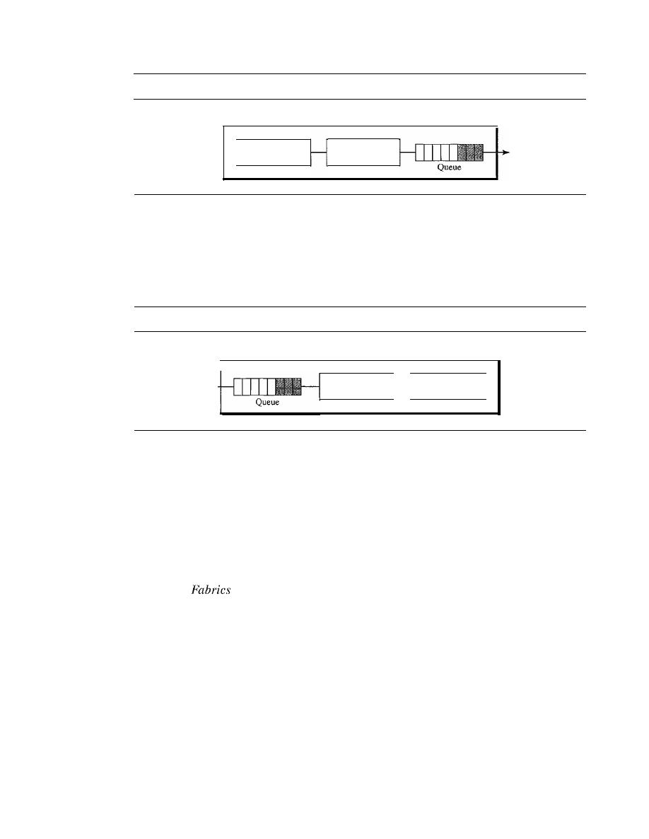
SECTION
8.4
STRUCTURE OF A SWITCH
233
Figure 8.22
Input port
Input port
Physical layer
processor
Data link layer
processor
Output Port
The output port performs the same functions as the input port, but in the reverse order.
First the outgoing packets are queued, then the packet is encapsulated in a frame, and
finally the physical layer functions are applied to the frame to create the signal to be
sent on the line. Figure 8.23 shows a schematic diagram of an output port.
Figure 8.23
Output port
Output port
Data link layer
processor
Physical layer
processor
ROllting Processor
The routing processor performs the functions of the network layer. The destination
address is used to find the address of the next hop and, at the same time, the output port
number from which the packet is sent out. This activity is sometimes referred to as
table lookup
because the routing processor searches the routing table. In the newer
packet switches, this function of the routing processor is being moved to the input ports
to facilitate and expedite the process.
Switching
The most difficult task in a packet switch is to move the packet from the input queue to
the output queue. The speed with which this is done affects the size of the input/output
queue and the overall delay in packet delivery. In the past, when a packet switch was
actually a dedicated computer, the memory of the computer or a bus was used as the
switching fabric. The input port stored the packet in memory; the output port retrieved
the packet from memory. Today, packet switches are specialized mechanisms that use a
variety of switching fabrics. We briefly discuss some of these fabrics here.
Crossbar
Switch
The simplest type of switching fabric is the crossbar switch, dis-
cussed in the previous section.
Banyan
Switch
A more realistic approach than the crossbar switch is the banyan
switch
(named after the banyan tree). A banyan switch is a multistage switch with
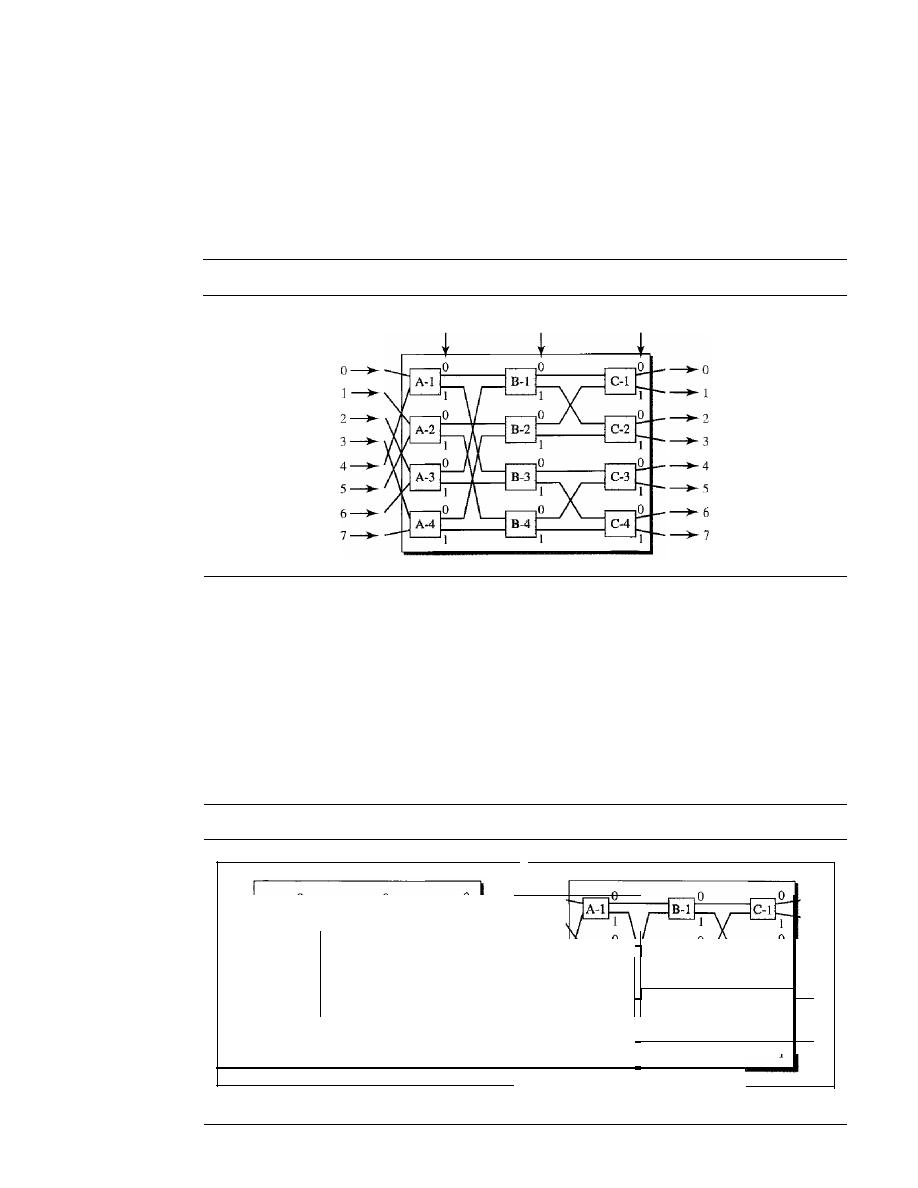
234
CHAPTER
8
SWITCHING
microswitches at each stage that route the packets based on the output port represented as
a binary string. For n inputs and n outputs, we have log2 n stages with nl2 microswitches
at each stage. The first stage routes the packet based on the high-order bit of the binary
string. The second stage routes the packet based on the second high-order bit, and so on.
Figure 8.24 shows a banyan switch with eight inputs and eight outputs. The number of
stages is Iog2(8)
=
3.
Figure 8.24
A banyan switch
Left bit
Middle bit
Right bit
Figure 8.25 shows the operation. In part a, a packet has arrived at input port 1 and
must go to output port 6 (110 in binary). The first microswitch
(A-2)
routes the packet
based on the first bit (1), the second microswitch (B-4) routes the packet based on the
second bit
(1),
and the third microswitch (C-4) routes the packet based on the third bit (0).
In part b, a packet has arrived at input port 5 and must go to output port 2 (010 in
binary). The first microswitch
(A-2)
routes the packet based on the first bit (0), the sec-
ond microswitch
(B-2)
routes the packet based on the second bit
(l),
and the third
microswitch
(C-2)
routes the packet based on the third bit (0).
Figure 8.25
Examples of routing in a banyan switch
0
0
0
0
1
1
1
I
2
2
2
2
3
3
3
3
4
4
4
4
5
5
5
5
6
6
6
6
7
7
7
7
a. Input 1 sending a cell to output 6 (110)
b. Input 5 sending a cell to output 2 (010)
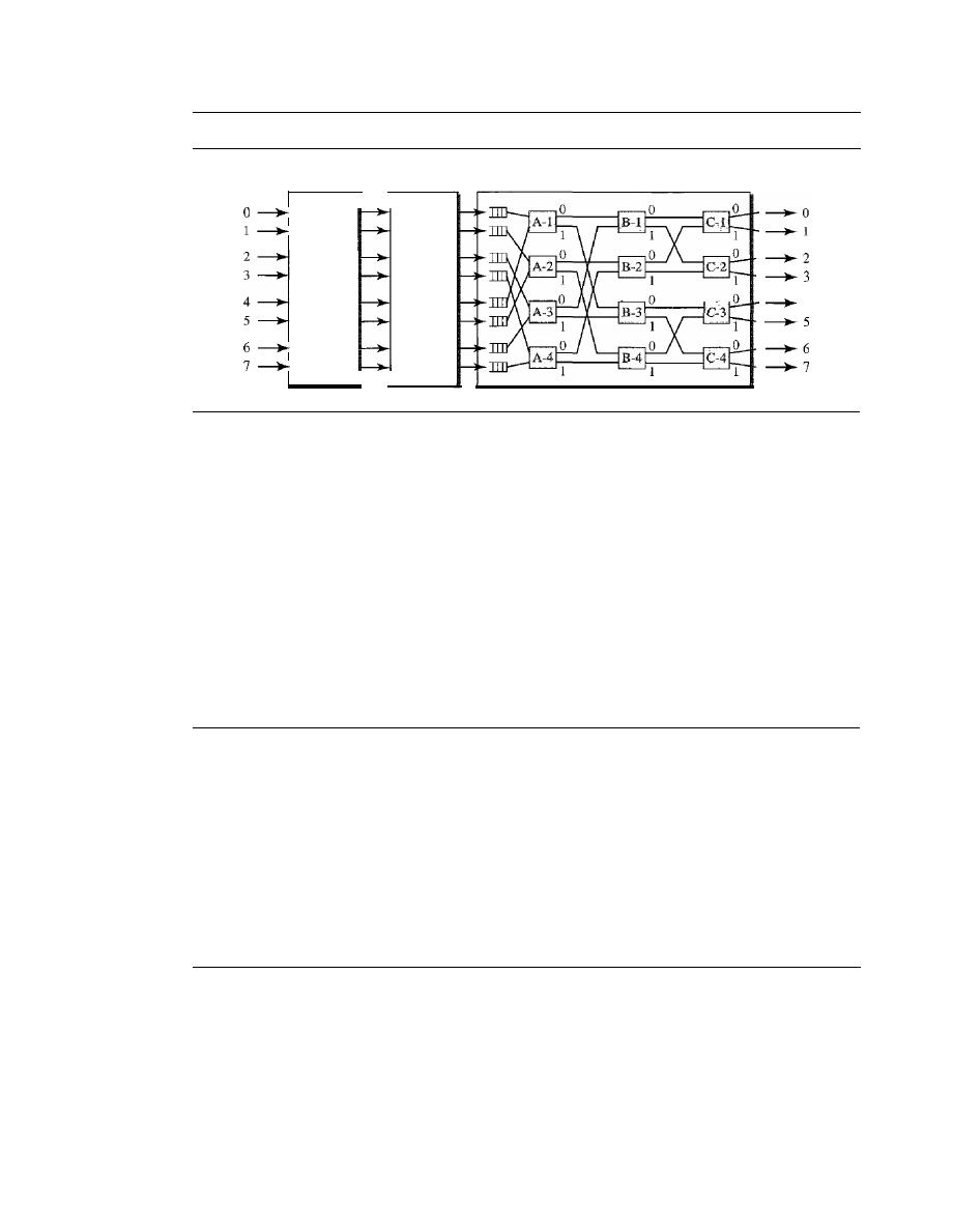
SECTION
8.6
KEY TERMS
235
Figure 8.26
Batcher-banyan switch
Banyan switch
Batcher
switch
Trap
module
4
Batcher-Banyan Switch
The problem with the banyan switch is the possibility of
internal collision even when two packets are not heading for the same output port. We
can solve this problem by sorting the arriving packets based on their destination port.
K.
E.
Batcher designed a switch that comes before the banyan switch and sorts the
incoming packets according to their final destinations. The combination is called the
Batcher-banyan switch.
The sorting switch uses hardware merging techniques, but we
do not discuss the details here. Normally, another hardware module called a trap is
added between the Batcher switch and the banyan switch (see Figure 8.26) The trap
module prevents duplicate packets (packets with the same output destination) from
passing to the banyan switch simultaneously. Only one packet for each destination is
allowed at each tick; if there is more than one, they wait for the next tick.
8.5
RECOMMENDED READING
For more details about subjects discussed in this chapter, we recommend the following
books. The items in brackets [...] refer to the reference list at the end of the text.
Books
Switching is discussed in Chapter 10 of [Sta04] and Chapters 4 and 7 of [GW04]. Circuit-
switching is fully discussed in [BELOO].
8.6
KEY TERMS
banyan switch
Batcher-banyan switch
blocking
circuit switching
circuit-switched network
crossbar switch
crosspoint
data transfer phase
datagram
datagram network
end system
input port

236
CHAPTER
8
SWITCHING
multistage switch
output port
packet-switched network
routing processor
setup phase
space-division switching
switch
switching
switching fabric
table lookup
teardown phase
time-division switching
time-slot interchange (TSI)
time-space-time (TST)
switch
trap
virtual-circuit identifier (VCI)
virtual-circuit network
8.7
SUMMARY
o
A switched network consists of a series of interlinked nodes, called switches. Tradi-
tionally' three methods of switching have been important: circuit switching, packet
switching, and message switching.
o
We can divide today's networks into three broad categories: circuit-switched networks,
packet-switched networks, and message-switched. Packet-switched networks can also
be divided into two subcategories: virtual-circuit networks and datagram networks
o
A circuit-switched network is made of a set of switches connected by physical links,
in which each link is divided into n channels. Circuit switching takes place at the
physical layer. In circuit switching, the resources need to be reserved during the
setup phase; the resources remain dedicated for the entire duration of data transfer
phase until the teardown phase.
o
In packet switching, there is no resource allocation for a packet. This means that
there is no reserved bandwidth on the links, and there is no scheduled processing
time for each packet. Resources are allocated on demand.
o
In a datagram network, each packet is treated independently of all others. Packets in
this approach are referred to as datagrams. There are no setup or teardown phases.
o
A virtual-circuit network is a cross between a circuit-switched network and a data-
gram network. It has some characteristics of both.
o
Circuit switching uses either of two technologies: the space-division switch or the
time-division switch.
o
A switch in a packet-switched network has a different structure from a switch used in
a circuit-switched network.We can say that a packet switch has four types of compo-
nents: input ports, output ports, a routing processor, and switching fabric.
8.8
PRACTICE SET
Review Questions
I.
Describe the need for switching and define a switch.
2. List the three traditional switching methods. What are the most common today?

SECTION
8.8
PRACTICE SET
237
3. What are the two approaches to packet-switching?
4. Compare and contrast a circuit-switched network and a packet-switched network.
5. What is the role of the address field in a packet traveling through a datagram
network?
6. What is the role of the address field in a packet traveling through a virtual-circuit
network?
7. Compare space-division and time-division switches.
8. What is TSI and its role in a time-division switching?
9. Define blocking in a switched network.
10. List four major components of a packet switch and their functions.
Exercises
11. A path in a digital circuit-switched network has a data rate of
I
Mbps. The exchange
of 1000 bits is required for the setup and teardown phases. The distance between
two parties is 5000 km. Answer the following questions if the propagataion speed is
2
X
10
8
m:
a. What is the total delay if 1000 bits of data are exchanged during the data transfer
phase?
b. What is the total delay if 100,000 bits of data are exchanged during the data
transfer phase?
c. What is the total delay if 1,000,000 bits of data are exchanged during the data
transfer phase?
d. Find the delay per 1000 bits of data for each of the above cases and compare
them. What can you infer?
12. Five equal-size datagrams belonging to the same message leave for the destina-
tion one after another. However, they travel through different paths as shown in
Table 8.1.
Table 8.1
Exercise 12
Datagram
Path Length
Visited Switches
1
3200Km
1,3,5
2
11,700 Km
1,2,5
3
12,200
Km
1,2,3,5
4
10,200
Km
1,4,5
5
10,700 Km
1,4,3,5
We assume that the delay for each switch (including waiting and processing) is 3,
10, 20, 7, and 20 ms respectively. Assuming that the propagation speed is 2 x 10
8
m,
find the order the datagrams arrive at the destination and the delay for each. Ignore
any other delays in transmission.

238
CHAPTER 8
SWITCHING
13. Transmission of information in any network involves end-to-end addressing and
sometimes local addressing (such as YCI). Table 8.2 shows the types of networks
and the addressing mechanism used in each of them.
Table
8.2
Exercise 13
Network
Setup
Data Transfer
Teardown
Circuit-switched
End-ta-end
End-ta-end
Datagram
End-ta-end
Virtual-circuit
End-to-end
Local
End-to-end
Answer the following questions:
a. Why does a circuit-switched network need end-to-end addressing during the setup
and teardown phases? Why are no addresses needed during the data transfer phase
for this type of network?
b. Why does a datagram network need only end-to-end addressing during the data
transfer phase, but no addressing during the setup and teardown phases?
c. Why does a virtual-circuit network need addresses during all three phases?
14. We mentioned that two types of networks, datagram and virtual-circuit, need a
routing or switching table to find the output port from which the information
belonging to a destination should be sent out, but a circuit-switched network has
no need for such a table. Give the reason for this difference.
15. An entry in the switching table of a virtual-circuit network is normally created
during the setup phase and deleted during the teardown phase. In other words, the
entries in this type of network reflect the current connections, the activity in the
network. In contrast, the entries in a routing table of a datagram network do not
depend on the current connections; they show the configuration of the network and
how any packet should be routed to a final destination. The entries may remain
the same even if there is no activity in the network. The routing tables, however, are
updated if there are changes in the network. Can you explain the reason for these
two different characteristics? Can we say that a virtual-circuit is a connection-
oriented
network and a datagram network is a connectionLess network because of the
above characteristics?
16. The minimum number of columns in a datagram network is two; the minimum num-
ber of columns in a virtual-circuit network is four. Can you explain the reason? Is the
difference related to the type of addresses carried in the packets of each network?
17. Figure 8.27 shows a switch (router) in a datagram network.
Find the output port for packets with the following destination addresses:
Packet 1: 7176
Packet 2: 1233
Packet 3: 8766
Packet 4: 9144
18. Figure 8.28 shows a switch in a virtual circuit network.
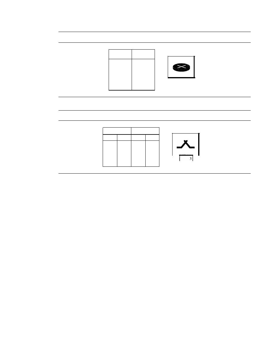
SECTION
8.8
PRACTICE SET
239
Figure 8.27
Exercise 17
Destination
Output
address
port
1233
3
1456
2
3255
1
4470
4
7176
2
8766
3
9144
2
4
2
3
Figure 8.28
Exercise 18
Incoming
Outgoing
Port
VCI
Port
VCI
1
14
3
22
2
71
4
41
2
92
1
45
3
58
2
43
3
78
2
70
4
56
3
11
2
4
Find the output port and the output VCI for packets with the following input port
and input VCI addresses:
Packet 1: 3, 78
Packet 2: 2, 92
Packet 3: 4, 56
Packet 4: 2, 71
19.
Answer the following questions:
a. Can a routing table in a datagram network have two entries with the same destina-
tion address? Explain.
b. Can a switching table in a virtual-circuit network have two entries with the same
input port number? With the same output port number? With the same incoming
VCls? With the same outgoing VCls? With the same incoming values (port, VCI)?
With the same outgoing values (port, VCI)?
20.
It
is obvious that a router or a switch needs to do searching to find information in
the corresponding table. The searching in a routing table for a datagram network is
based on the destination address; the searching in a switching table in a virtual-
circuit network is based on the combination of incoming port and incoming VCI.
Explain the reason and define how these tables must be ordered (sorted) based on
these values.
2]. Consider an n
X
k
crossbar switch with n inputs and
k
outputs.
a. Can we say that switch acts as a multiplexer if
n
>
k?
b. Can we say that switch acts as a demultiplexer if
n
<
k?

240
CHAPTER
8
SWITCHING
22. We need a three-stage space-division switch with N
=
100. We use 10 crossbars at
the first and third stages and 4 crossbars at the middle stage.
a. Draw the configuration diagram.
b. Calculate the total number of crosspoints.
c. Find the possible number of simultaneous connections.
d. Find the possible number of simultaneous connections if we use one single cross-
bar (100 x 100).
e. Find the blocking factor, the ratio of the number of connections in c and in d.
23. Repeat Exercise 22 if we use 6 crossbars at the middle stage.
24. Redesign the configuration of Exercise 22 using the Clos criteria.
25. We need to have a space-division switch with 1000 inputs and outputs. What is the
total number of crosspoints in each of the following cases?
a. Using one single crossbar.
b. Using a multi-stage switch based on the Clos criteria
26. We need a three-stage time-space-time switch with N
=
100. We use 10 TSIs at the
first and third stages and 4 crossbars at the middle stage.
a. Draw the configuration diagram.
b. Calculate the total number of crosspoints.
c. Calculate the total number of memory locations we need for the TSIs.

CHAPTER 9
Using Telephone and Cable Networks
for Data Transmission
Telephone networks were originally created to provide voice communication. The need
to communicate digital data resulted in the invention of the dial-up modem. With the
advent of the Internet came the need for high-speed downloading and uploading; the
modem was just too slow. The telephone companies added a new technology, the
digital
subscriber line (DSL). Although dial-up modems still exist in many places all over the
world, DSL provides much faster access to the Internet through the telephone network.
In this chapter, we first discuss the basic structure of the telephone network. We then see
how dial-up modems and DSL technology use these networks to access the Internet.
Cable networks were originally created to provide access to TV programs for those
subscribers who had no reception because of natural obstructions such as mountains.
Later the cable network became popular with people who just wanted a better signal. In
addition, cable networks enabled access to remote broadcasting stations via microwave
connections. Cable TV also found a good market in Internet access provision using
some of the channels originally designed for video. After discussing the basic structure
of cable networks, we discuss how cable modems can provide a high-speed connection
to the Internet.
9.1
TELEPHONE NETWORK
Telephone networks use circuit switching. The telephone network had its beginnings
in the late 1800s. The entire network, which is referred to as the
plain old telephone
system (POTS),
was originally an analog system using analog signals to transmit voice.
With the advent of the computer era, the network, in the 1980s, began to carry data in
addition to voice. During the last decade, the telephone network has undergone many
technical changes. The network is now digital as well as analog.
Major Components
The telephone network, as shown in Figure 9.1, is made of three major components:
local loops, trunks, and switching offices. The telephone network has several levels of
switching offices such as
end offices, tandem offices,
and
regional offices.
241
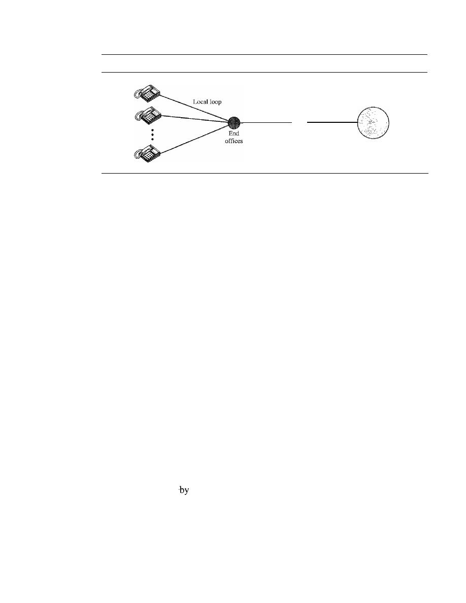
242
CHAPTER
9
USING 1ELEPHONE AND CABLE NETWORKS FOR DATA TRANSMISSION
Figure 9.1
A telephone system
Trunk
Tandem
offices
Trunk
Regional offices
Local Loops
One component of the telephone network is the
local loop,
a twisted-pair cable that con-
nects the subscriber telephone to the nearest end office or local central office. The local
loop, when used for voice, has a bandwidth of
4000
Hz
(4
kHz).
It
is interesting to examine
the telephone number associated with each local loop. The first three digits of a local tele-
phone number define the office, and the next four digits define the local loop number.
Trunks
Trunks
are transmission media that handle the communication between offices. A
trunk normally handles hundreds or thousands of connections through multiplexing.
Transmission is usually through optical fibers or satellite links.
Switching Offices
To avoid having a permanent physical link between any two subscribers, the telephone
company has switches located in a
switching office.
A switch connects several local
loops or trunks and allows a connection between different subscribers.
LATAs
After the divestiture of 1984 (see Appendix E), the United States was divided into more
than
200 local-access transport areas (LATAs).
The number of LATAs has increased
since then. A LATA can be a small or large metropolitan area. A small state may have one
single LATA; a large state may have several LATAs. A LATA boundary may overlap the
boundary of a state; part of a LATA can be in one state, part in another state.
Intra-LATA Services
The services offered
the
common carriers
(telephone companies) inside a LATA are
called
intra-LATA services. The carrier that handles these services is called a
local
exchange carrier (LEC).
Before the Telecommunications Act of 1996 (see Appendix
E),
intra-LATA services were granted to one single carrier. This was a monopoly. After 1996,
more than one carrier could provide services inside a LATA. The carrier that provided ser-
vices before 1996 owns the cabling system (local loops) and is called the
incumbent local
exchange carrier (ILEC).
The new carriers that can provide services are called
competitive local exchange carriers (CLECs).
To avoid the costs of new cabling, it
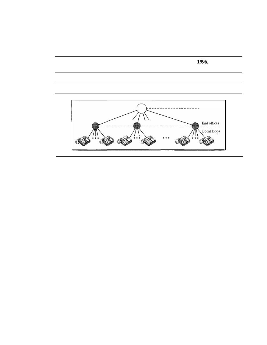
SECTION 9.1
TELEPHONE NETWORK
243
was agreed that the ILECs would continue to provide the main services, and the CLECs
would provide other services such as mobile telephone service, toll calls inside a LATA,
and so on. Figure 9.2 shows a LATA and switching offices.
Intra-LATA services are provided by local exchange carriers. Since
there are two
types ofLECs: incumbent local exchange carriers and competitive local exchange carriers.
Figure 9.2
Switching offices in a LATA
Tandem (toll) offices
Communication inside a LATA is handled by end switches and tandem switches. A
call that can be completed by using only end offices is considered toll-free. A call that
has to go through a tandem office (intra-LATA toll office) is charged.
Inter-LATA Services
The services between LATAs are handled by
interexchange carriers (IXCs).
These
carriers, sometimes called
long-distance companies,
provide communication services
between two customers in different LATAs. After the act of 1996 (see Appendix E),
these services can be provided by any carrier, including those involved in intra-LATA
services. The field is wide open. Carriers providing inter-LATA services include AT&T,
MCI, WorldCom, Sprint, and Verizon.
The IXCs are long-distance carriers that provide general data communications ser-
vices including telephone service. A telephone call going through an IXC is normally
digitized, with the carriers using several types of networks to provide service.
Points of Presence
As we discussed, intra-LATA services can be provided by several LECs (one ILEC and
possibly more than one CLEC). We also said that inter-LATA services can be provided
by several IXCs. How do these carriers interact with one another? The answer is, via a
switching office called a point
of presence
(POP). Each IXC that wants to provide inter-
LATA services in a LATA must have a POP in that LATA. The LECs that provide services
inside the LATA must provide connections so that every subscriber can have access to all
POPs. Figure 9.3 illustrates the concept.
A subscriber who needs to make a connection with another subscriber is connected
first to an end switch and then, either directly or through a tandem switch, to a POP. The
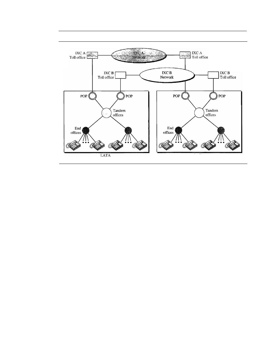
244
CHAPTER
9
USING TELEPHONE AND CABLE NETWORKS FOR DATA TRANSMISSION
Figure 9.3
Point ofpresences (POPs)
LATA
call now goes from the POP of an IXC (the one the subscriber has chosen) in the source
LATA to the POP of the same IXC in the destination LATA. The call is passed through
the toll office of the IXC and is carried through the network provided by the IXC.
Signaling
The telephone network, at its beginning, used a circuit-switched network with dedicated
links (multiplexing had not yet been invented) to transfer voice communication. As we
saw in Chapter 8, a circuit-switched network needs the setup and teardown phases to
establish and terminate paths between the two communicating parties. In the beginning,
this task was performed by human operators. The operator room was a center to which
all subscribers were connected. A subscriber who wished to talk to another subscriber
picked up the receiver (off-hook) and rang the operator. The operator, after listening to
the caller and getting the identifier of the called party, connected the two by using a wire
with two plugs inserted into the corresponding two jacks. A dedicated circuit was created
in this way. One of the parties, after the conversation ended, informed the operator to
disconnect the circuit. This type of signaling is called
in-band signaling
because the same
circuit can be used for both signaling and voice communication.
Later, the signaling system became automatic. Rotary telephones were invented that
sent a digital signal defining each digit in a multidigit telephone number. The switches in
the telephone companies used the digital signals to create a connection between the caller
and the called parties. Both in-band and
out-of-band signaling
were used. In in-band
signaling, the 4-kHz voice channel was also used to provide signaling. In out-of-band
signaling, a portion of the voice channel bandwidth was used for signaling; the voice
bandwidth and the signaling bandwidth were separate.

SECTION
9.1
TELEPHONE NETWORK
245
As telephone networks evolved into a complex network, the functionality of the sig-
naling system increased. The signaling system was required to perform other tasks such as
1. Providing dial tone, ring tone, and busy tone
2. Transferring telephone numbers between offices
3. Maintaining and monitoring the call
4. Keeping billing information
5. Maintaining and monitoring the status of the telephone network equipment
6. Providing other functions such as caller ID, voice mail, and so on
These complex tasks resulted in the provision of a separate network for signaling. This
means that a telephone network today can be thought of as two networks: a signaling
network and a data transfer network.
The tasks of data transfer and signaling are separated in modern telephone networks:
data transfer is done
by
one network, signaling
by
another.
However, we need to emphasize a point here. Although the two networks are separate,
this does not mean that there are separate physical links everywhere; the two networks
may use separate channels of the same link in parts of the system.
Data Transfer Network
The data transfer network that can carry multimedia information today is, for the most
part, a circuit-switched network, although it can also be a packet-switched network. This
network follows the same type of protocols and model as other networks discussed in
this book.
Signaling Network
The signaling network,
is our main concern in this section, is a packet-switched
network involving the layers similar to those in the OSI model or Internet model, dis-
cussed in Chapter 2. The nature of signaling makes it more suited to a packet-switching
network with different layers. For example, the information needed to convey a telephone
address can easily be encapsulated in a packet with all the error control and addressing
information. Figure 9.4 shows a simplified situation of a telephone network in which the
two networks are separated.
The user telephone or computer is connected to the signal points (SPs). The link
between the telephone set and SP is common for the two networks. The signaling net-
work uses nodes called signal transport ports (STPs) that receive and forward signaling
messages. The signaling network also includes a service control point (SCP) that con-
trols the whole operation of the network. Other systems such as a database center may
be included to provide stored information about the entire signaling network.
Signaling System Seven (5S7)
The protocol that is used in the signaling network is called Signaling System Seven (SS7).
It
is very similar to the five-layer Internet model we saw in Chapter 2, but the layers have
different names, as shown in Figure 9.5.
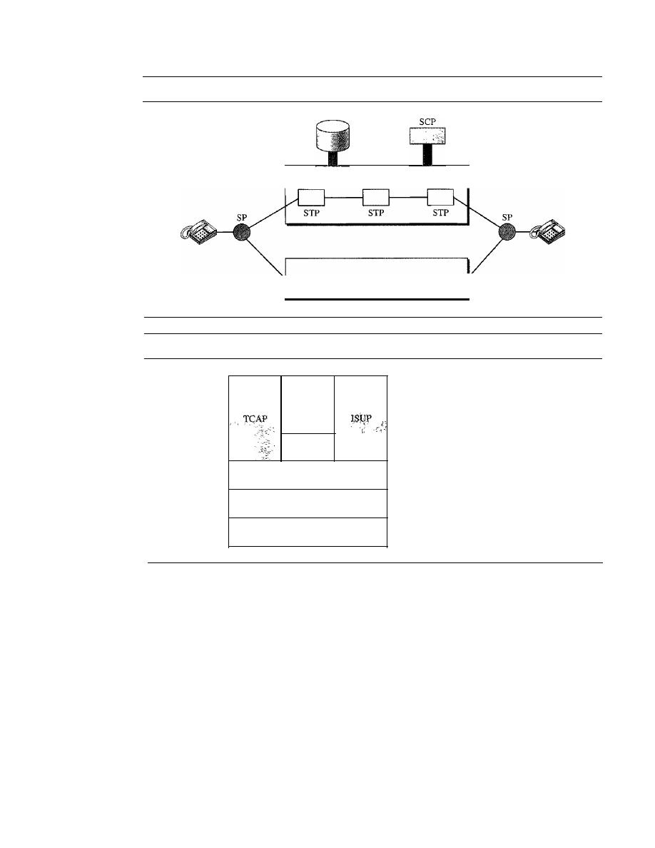
246
CHAPTER
9
USING TELEPHONE AND CABLE NETWORKS FOR DATA TRANSMISSION
Figure 9.4
Data transfer and signaling networks
SP: Signal point
STP: Signal transfer point
Database
Figure 9.5
Layers in SS7
Signaling network
Data transfer network
Upper layers
__
Network layer
Data link layer
Physical layer
TUP
SCCP
MTP level 3
MTPIevel2
MTPlevell
MTP: Message transfer part
SCCP: Signaling connection control point
TeAP: Transaction capabilities application port
TUP: Telephone user port
ISUP: ISDN user port
Physical Layer: MTP Level 1
The physical layer in SS7 called message transport
part (MTP) level
I
uses several physical layer specifications such as T-l (1.544 Mbps)
and DCa (64 kbps).
Data Link Layer: MTP Level 2
The MTP level 2 layer provides typical data link
layer services such as packetizing, using source and destination address in the packet
header, and CRC for error checking.
Network Layer: MTP Level 3
The MTP level 3 layer provides end-to-end connectivity
by using the datagram approach to switching. Routers and switches route the signal packets
from the source to the destination.
Transport Layer: SCCP
The signaling connection control point (SCCP) is used
for special services such as SaO-call processing.
Upper Layers: TUP, TCAP, and ISUP
There are three protocols at the upper layers.
Telephone user port (TUP) is responsible for setting up voice calls.
It
receives the dialed

SECTION
9.1
TELEPHONE NETWORK
247
digits and routes the calls. Transaction capabilities application port (TCAP) provides
remote calls that let an application program on a computer invoke a procedure on another
computer. ISDN user port (ISUP) can replace TUP to provide services similar to those
of an ISDN network.
Services Provided
by
Telephone Networks
Telephone companies provide two types of services: analog and digital.
Analog Services
In the beginning, telephone companies provided their subscribers with analog services.
These services still continue today. We can categorize these services as either analog
switched services or analog leased services.
Analog Switched Services
This is the familiar dial-up service most often encountered
when a home telephone is used. The signal on a local loop is analog, and the bandwidth is
usually between
0
and
4000
Hz. A local call service is normally provided for a flat monthly
rate, although in some LATAs, the carrier charges for each call or a set of calls. The rationale
for a non flat-rate charge is to provide cheaper service for those customers who do not
make many calls. A toll call can be intra-LATA or inter-LATA.
If
the LATA is geographi-
cally large, a call may go through a tandem office (toll office) and the subscriber will pay a
fee for the call. The inter-LATA calls are long-distance calls and are charged as such.
Another service is called
800
service.
If
a subscriber (normally an organization)
needs to provide free connections for other subscribers (normally customers),
it
can
request the 800 service. In this case, the call is free for the caller, but it is paid by the
callee. An organization uses this service to encourage customers to call. The rate is less
expensive than that for a normal long-distance call.
The wide-area telephone service (WATS) is the opposite of the
800
service. The
latter are inbound calls paid by the organization; the former are outbound calls paid by
the organization. This service is a less expensive alternative to regular toll calls;
charges are based on the number of calls. The service can be specified as outbound
calls to the same state, to several states, or to the whole country, with rates charged
accordingly.
The 900 services are like the
800
service, in that they are inbound calls to a sub-
scriber. However, unlike the
800
service, the call is paid by the caller and is normally
much more expensive than a normal long-distance call. The reason is that the carrier
charges two fees: the first is the long-distance toll, and the second is the fee paid to the
callee for each call.
Analog Leased Service
An analog leased service offers customers the opportunity
to lease a line, sometimes called a dedicated line, that is permanently connected to
another customer. Although the connection still passes through the switches in the tele-
phone network, subscribers experience it as a single line because the switch is always
closed; no dialing is needed.
Digital Services
Recently telephone companies began offering digital services to their subscribers. Digital
services are less sensitive than analog services to noise and other forms of interference.
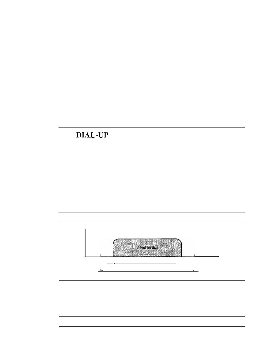
248
CHAPTER
9
USING TELEPHONE AND CABLE NETWORKS FOR DATA TRANSMISSION
The two most common digital services are switched/56 service and digital data service
(DDS). We already discussed high-speed digital services-the T lines-in Chapter 6. We
discuss the other services in this chapter.
Switched/56 Service
Switched/56 service is the digital version of an analog switched
line. It is a switched digital service that allows data rates of up to 56 kbps. To communi-
cate through this service, both parties must subscribe. A caller with normal telephone
service cannot connect to a telephone or computer with switched/56 service even if the
caller is using a modem. On the whole, digital and analog services represent two com-
pletely different domains for the telephone companies. Because the line in a switched!
56 service is already digital, subscribers do not need modems to transmit digital data.
However, they do need another device called a digital service unit (DSU).
Digital Data Service
Digital data service (DDS) is the digital version of an analog
leased line; it is a digital leased line with a maximum data rate of 64 kbps.
9.2
MODEMS
Traditional telephone lines can carry frequencies between 300 and 3300 Hz, giving
them a bandwidth of 3000 Hz. All this range is used for transmitting voice, where a
great deal of interference and distortion can be accepted without loss of intelligibility.
As we have seen, however, data signals require a higher degree of accuracy to ensure
integrity. For safety's sake, therefore, the edges of this range are not used for data com-
munications. In general, we can say that the signal bandwidth must be smaller than the
cable bandwidth. The effective bandwidth of a telephone line being used for data trans-
mission is 2400 Hz, covering the range from 600 to 3000 Hz. Note that today some
telephone lines are capable of handling greater bandwidth than traditional lines. How-
ever, modem design is still based on traditional capability (see Figure 9.6).
Figure 9.6
Telephone line bandwidth
Used for voice
300
600
2400 Hz for data
3300
I
I
I
I
I
I
3000 Hz for voice
I
I
I
I
The term modem is a composite word that refers to the two functional entities that
make up the device: a signal modulator and a signal demodulator. A modulator creates
a bandpass analog signal from binary data. A demodulator recovers the binary data
from the modulated signal.
Modem stands for modulator/demodulator.
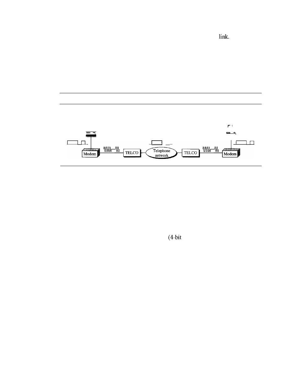
SECTION
9.2
DIAL-UP MODEMS
249
Figure 9.7 shows the relationship of modems to a communications
The computer
on the left sends a digital signal to the modulator portion of the modem; the data are sent as
an analog signal on the telephone lines. The modem on the right receives the analog signal,
demodulates it through its demodulator, and delivers data to the computer on the right. The
communication can be bidirectional, which means the computer on the right can simulta-
neously send data to the computer on the left, using the same modulation/demodulation
processes.
Figure 9.7
Modulation/demodulation
TELCO: Telephone company
A
Modem Standards
n
B
Today, many of the most popular modems available are based on the V-series standards
published by the ITU-T. We discuss just the most recent series.
V.32 and V.32bis
The V.32 modem uses a combined modulation and encoding technique called trellis-
coded modulation. Trellis is essentially QAM plus a redundant bit. The data stream is
divided into 4-bit sections. Instead of a quadbit
pattern), however, a
pentabit
(5-bit
pattern) is transmitted. The value of the extra bit is calculated from the values of the
data bits. The extra bit is used for error detection.
The Y.32 calls for 32-QAM with a baud rate of 2400. Because only 4 bits of each
pentabit represent data, the resulting data rate is 4 x 2400
=
9600 bps. The constellation
diagram and bandwidth are shown in Figure 9.8.
The V.32bis modem was the first of the ITU-T standards to support 14,400-bps
transmission. The Y.32bis uses 128-QAM transmission (7 bits/baud with I bit for error
control) at a rate of 2400 baud (2400 x 6
=
14,400 bps).
An additional enhancement provided by Y.32bis is the inclusion of an automatic
fall-back and fall-forward feature that enables the modem to adjust its speed upward or
downward depending on the quality of the line or signal. The constellation diagram and
bandwidth are also shown in Figure 9.8.
V.
34bis
The V.34bis modem provides a bit rate of 28,800 with a 960-point constellation and a
bit rate of 33,600 bps with a 1664-point constellation.
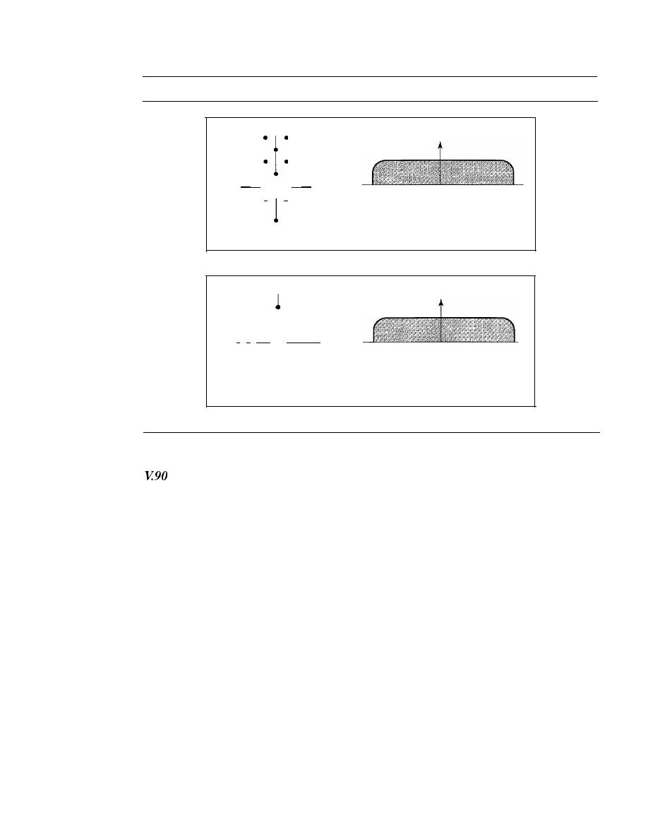
250
CHAPTER
9
USING TELEPHONE AND CABLE NETWORKS FOR DATA TRANSMISSION
Figure 9.8
The V.32 and V.32bis constellation and bandwidth
90
Full-duplex 2400-baud
•
•
9600-bps 2-wire
•
•
•
•
•
•
•
•
180
•
·i ·
•
0
600
1800
3000
•
•
•
•
•
• •
•
•
•
• I
•
270
a. Constellation and bandwidth for V.32
90
• •
• • • •
••
••
• • • • •
•
•
••
•
••
• • • • • •
•
•
•
•
••
••••
• • • • • • •
•
•
•
•
•
••
••••
180 • • • •
• • • • 0
•
•
•
•
•
•
•
•
•
•
• •
••
••••
•
•
•
•
•
•
•
•
• ••
•••
•
•
•
•
•
•
••
••
•
•
•
•
•
•
270
Full-duplex. 2400-baud
14,400-bps 4-wire
600
1800
3000
b. Constellation and bandwidth for V.32bis
Traditional modems have a data rate limitation of 33.6 kbps, as determined by the
Shannon capacity (see Chapter 3). However, V.90 modems with a bit rate of 56,000 bps
are available; these are called 56K modems. These modems may be used only if one
party is using digital signaling (such as through an Internet provider). They are asym-
metric in that the downloading rate (flow of data from the Internet service provider to
the PC) is a maximum of 56 kbps, while the uploading rate (flow of data from the PC to
the Internet provider) can be a maximum of 33.6 kbps. Do these modems violate the
Shannon capacity principle? No, in the downstream direction, the SNR ratio is higher
because there is no quantization error (see Figure 9.9).
In uploading, the analog signal must still be sampled at the switching station. In
this direction, quantization noise (as we saw in Chapter 4) is introduced into the signal,
which reduces the SNR ratio and limits the rate to 33.6 kbps.
However, there is no sampling in the downloading. The signal is not affected by
quantization noise and not subject to the Shannon capacity limitation. The maximum data
rate in the uploading direction is still 33.6 kbps, but the data rate in the downloading
direction is now 56 kbps.
One may wonder how we arrive at the 56-kbps figure. The telephone companies
sample 8000 times per second with 8 bits per sample. One of the bits in each sample is
used for control purposes, which means each sample is 7 bits. The rate is therefore
8000 x 7, or 56,000 bps or 56 kbps.
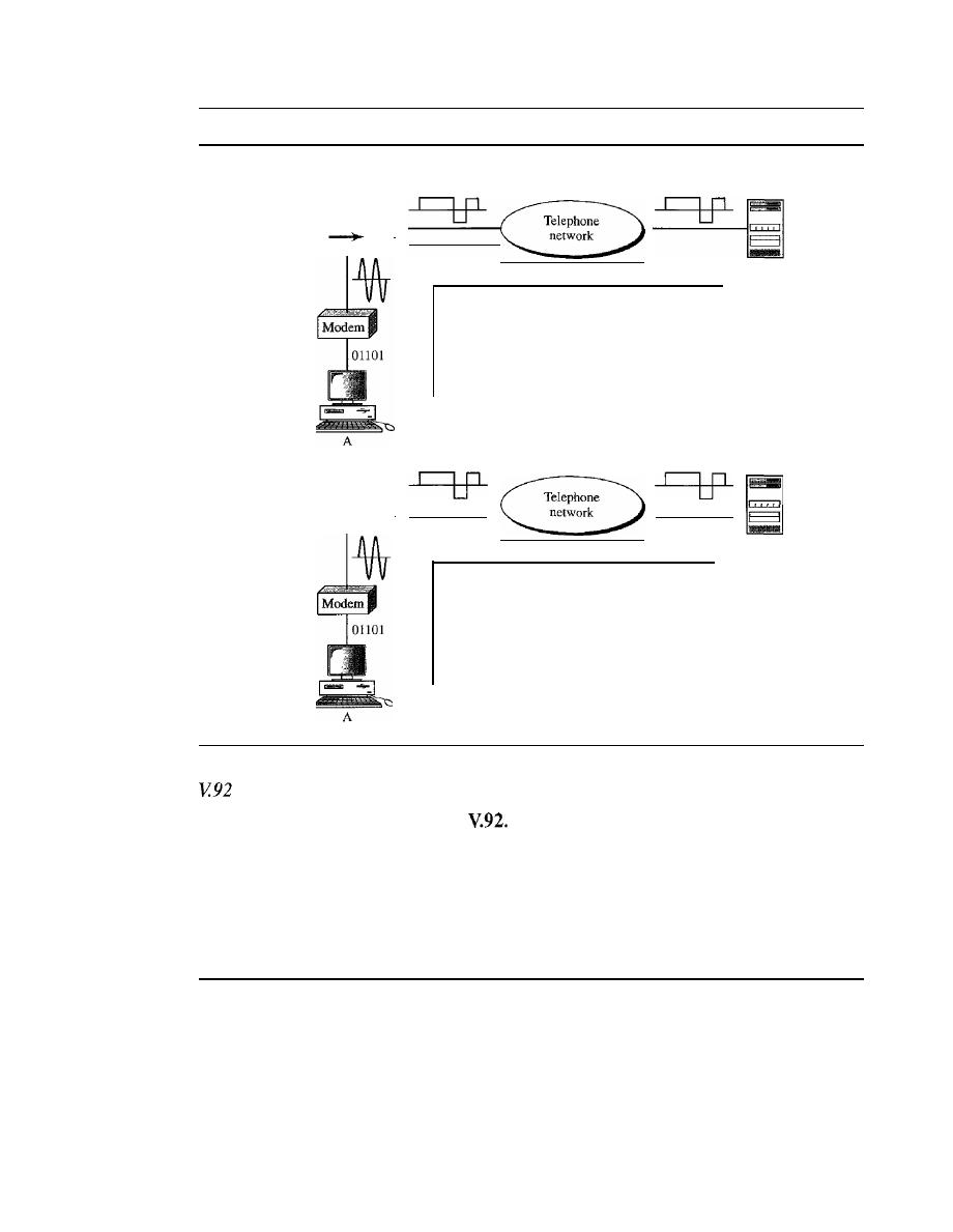
SECTION
9.3
DIGITAL SUBSCRIBER LINE
251
Figure 9.9
Uploading and downloading in 56K modems
Quantization noise limits
the data rate
1 - - - - - - - - 1
1
PCM
I
1
I
1
I
Uploading,
quantization noise
ISP
server
1 - - - - - - - - 1
1
Inverse
I
1
PCM
I
1
I
ISP
server
Downloading,
no quantization noise
The standard above V90 is called
These modems can adjust their speed, and if
the noise allows, they can upload data at the rate of 48 kbps. The downloading rate is
still 56 kbps. The modem has additional features. For example, the modem can inter-
rupt the Internet connection when there is an incoming call if the line has call-waiting
service.
9.3
DIGITAL SUBSCRIBER LINE
After traditional modems reached their peak data rate, telephone companies developed
another technology, DSL, to provide higher-speed access to the Internet. Digital sub-
scriber line (DSL) technology is one of the most promising for supporting high-speed
digital communication over the existing local loops. DSL technology is a set of tech-
nologies, each differing in the first letter (ADSL, VDSL, HDSL, and SDSL). The set is
often referred to as xDSL, where
x
can be replaced by A, V, H, or S.

252
CHAPTER
9
USING TELEPHONE AND CABLE NETWORKS FOR DATA TRANSMISSION
ADSL
The first technology in the set is
asymmetric
DSL (ADSL). ADSL, like a 56K modem,
provides higher speed (bit rate) in the downstream direction (from the Internet to the
resident) than in the upstream direction (from the resident to the Internet). That is the
reason
it
is called asymmetric. Unlike the asymmetry in 56K modems, the designers of
ADSL specifically divided the available bandwidth of the local loop unevenly for the
residential customer. The service is not suitable for business customers who need a
large bandwidth in both directions.
ADSL is an asymmetric communication technology designed for residential users;
it is not suitable for businesses.
Using Existing Local Loops
One interesting point is that ADSL uses the existing local loops. But how does ADSL
reach a data rate that was never achieved with traditional modems? The answer is that the
twisted-pair local loop is actually capable of handling bandwidths up to 1.1 MHz, but the
filter installed at the end office of the telephone company where each local loop termi-
nates limits the bandwidth to 4 kHz (sufficient for voice communication).
If
the filter is
removed, however, the entire 1.1 MHz is available for data and voice communications.
The existing local loops can handle bandwidths up to 1.1 MHz.
Adaptive Technology
Unfortunately, 1.1 MHz is just the theoretical bandwidth of the local loop. Factors such
as the distance between the residence and the switching office, the size of the cable, the
signaling used, and so on affect the bandwidth. The designers of ADSL technology
were aware of this problem and used an adaptive technology that tests the condition and
bandwidth availability of the line before settling on a data rate. The data rate of ADSL
is not fixed;
it
changes based on the condition and type of the local loop cable.
ADSL is an adaptive technology. The system uses a data rate
based on the condition of the local loop line.
Discrete Multitone Technique
The modulation technique that has become standard for ADSL is called the
discrete
multitone technique
(DMT) which combines QAM and FDM. There is no set way
that the bandwidth of a system is divided. Each system can decide on its bandwidth
division. Typically, an available bandwidth of 1.104 MHz is divided into 256 channels.
Each channel uses a bandwidth of 4.312 kHz, as shown in Figure 9.10. Figure 9.11 shows
how the bandwidth can be divided into the following:
o
Voice.
Channel 0 is reserved for voice communication.
o
Idle.
Channels 1 to 5 are not used and provide a gap between voice and data
communication.
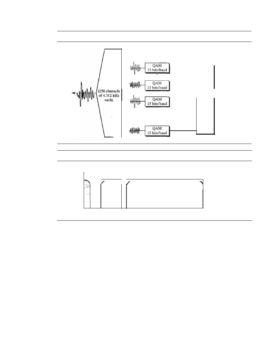
SECTION
9.3
DIGITAL SUBSCRIBER LINE
253
Figure 9.10
Discrete multitone technique
Upstream
bits
Downstream
bits
Figure 9.11
Bandwidth division in ADSL
Voice
Upstream
Downstream
Not
used
o
4
26
108 138
1104
kHz
o
Upstream data and control. Channels 6 to 30 (25 channels) are used for upstream
data transfer and control. One channel is for control, and 24 channels are for data
transfer.
If
there are 24 channels, each using 4 kHz (out of 4.312 kHz available)
with QAM modulation, we have 24 x 4000 x 15, or a 1.44-Mbps bandwidth, in
the upstream direction. However, the data rate is normally below 500 kbps because
some of the carriers are deleted at frequencies where the noise level is large. In other
words, some of channels may be unused.
o
Downstream data and control. Channels 31 to 255 (225 channels) are used for
downstream data transfer and control. One channel is for control, and 224 channels
are for data.
If
there are 224 channels, we can achieve up to 224 x 4000 x 15, or
13.4 Mbps. However, the data rate is normally below 8 Mbps because some of the
carriers are deleted at frequencies where the noise level is large. In other words,
some of channels may be unused.
Customer Site: ADSL Modem
Figure 9.12 shows an
ADSL modem installed at a customer's site. The local loop
connects to a splitter which separates voice and data communications. The ADSL
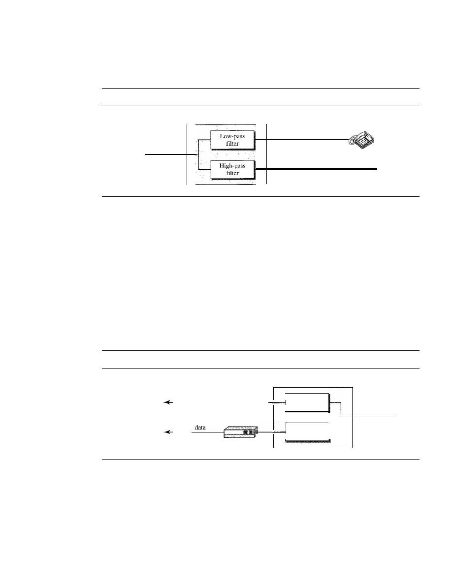
254
CHAPTER
9
USING TELEPHONE AND CABLE NETWORKS FOR DATA TRANSMISSION
modem modulates and demodulates the data, using DMT, and creates downstream
and upstream channels.
Figure 9.12
ADSL modem
Splitter
Local loop
Voice
Data
ADSLmodem
Note that the splitter needs to be installed at the customer's premises, normally by a
technician from the telephone company. The voice line can use the existing telephone
wiring in the house, but the data line needs to be installed by a professional. All this
makes the ADSL line expensive. We will see that there is an alternative technology,
Universal ADSL (or ADSL Lite).
Telephone Company Site: DSLAM
At the telephone company site, the situation is different. Instead of an ADSL modem, a
device called a
digital subscriber line access multiplexer
(DSLAM) is installed that
functions similarly. In addition, it packetizes the data to be sent to the Internet (ISP
server). Figure 9.13 shows the configuration.
Figure 9.13
DSLAM
Splitter
To telephone
V_o_ic_e_ _
network
Low-pass
filter
Local loop
High-pass
filter
Packetized
To the
_ _
Internet
ADSL Lite
The installation of splitters at the border of the premises and the new wiring for the data
line can be expensive and impractical enough to dissuade most subscribers. A new ver-
sion of ADSL technology called ADSL
Lite
(or Universal ADSL or splitterless ADSL) is
available for these subscribers. This technology allows an ASDL Lite modem to be
plugged directly into a telephone jack and connected to the computer. The splitting is
done at the telephone company. ADSL Lite uses 256 DMT carriers with 8-bit modulation

SECTION
9.3
DIGITAL SUBSCRIBER LINE
255
(instead of 15-bit). However, some of the carriers may not be available because errors
created by the voice signal might mingle with them.
It
can provide a maximum down-
stream data rate of 1.5 Mbps and an upstream data rate of 512 kbps.
HDSL
The high-bit-rate digital subscriber line (HDSL) was designed as an alternative to
the T-lline (1.544 Mbps). The T-1line uses alternate mark inversion (AMI) encoding,
which is very susceptible to attenuation at high frequencies. This limits the length of
a T-l line to 3200 ft
(1
km). For longer distances, a repeater is necessary, which means
increased costs.
HDSL uses 2B1Q encoding (see Chapter 4), which is less susceptible to attenuation.
A data rate of 1.544 Mbps (sometimes up to 2 Mbps) can be achieved without repeaters
up to a distance of 12,000
ft
(3.86 km). HDSL uses two twisted pairs (one pair for each
direction) to achieve full-duplex transmission.
SDSL
The symmetric digital subscriber line (SDSL) is a one twisted-pair version ofHDSL.
It
provides full-duplex symmetric communication supporting up to 768 kbps in each
direction. SDSL, which provides symmetric communication, can be considered an
alternative to ADSL. ADSL provides asymmetric communication, with a downstream
bit rate that is much higher than the upstream bit rate. Although this feature meets the
needs of most residential subscribers, it is not suitable for businesses that send and
receive data in large volumes in both directions.
VDSL
The very high-bit-rate digital subscriber line (VDSL), an alternative approach that is
similar to ADSL, uses coaxial, fiber-optic, or twisted-pair cable for short distances. The
modulating technique is DMT.
It
provides a range of bit rates (25 to 55 Mbps) for
upstream communication at distances of 3000 to 10,000 ft. The downstream rate is nor-
mally 3.2 Mbps.
Summary
Table 9.1 shows a summary of DSL technologies. Note that the data rate and distances
are approximations and can vary from one implementation to another.
Table 9.1
Summary of DSL technologies
Downstream
Upstream
Distance
Twisted
Line
Technology
Rate
Rate
(jt)
Pairs
Code
ADSL
1.5-6.1 Mbps
16-640 kbps
12,000
1
DMT
ADSL Lite
1.5 Mbps
500 kbps
18,000
1
DMT
HDSL
1.5-2.0 Mbps
1.5-2.0 Mbps
12,000
2
2B1Q
SDSL
768 kbps
768 kbps
12,000
1
2B1Q
VDSL
25-55 Mbps
3.2 Mbps
3000-10,000
1
DMT
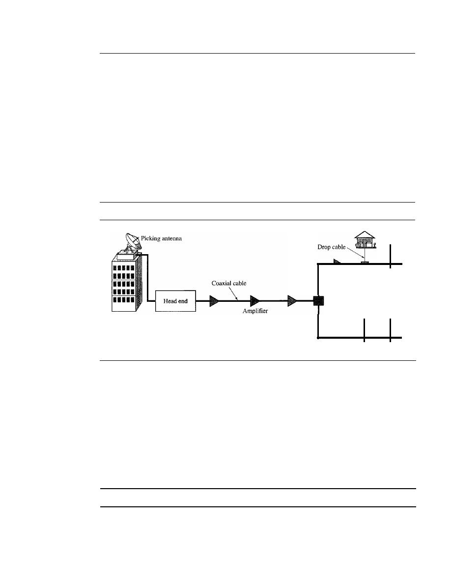
256
CHAPTER
9
USING TELEPHONE AND CABLE NETWORKS FOR DATA TRANSMISSION
9.4
CABLE TV NETWORKS
The
cable TV network
started as a video service provider, but it has moved to the business
of Internet access. In this section, we discuss cable TV networks per se; in Section 9.5 we
discuss how this network can be used to provide high-speed access to the Internet.
Traditional Cable Networks
Cable TV
started to distribute broadcast video signals to locations with poor or no
reception in the late 1940s.
It
was called
community antenna TV (CATV)
because an
antenna at the top of a tall hill or building received the signals from the TV stations and
distributed them, via coaxial cables, to the community. Figure 9.14 shows a schematic
diagram of a traditional cable TV network.
Figure 9.14
Traditional cable TV network
Splitter
Tap
The cable TV office, called the
head end,
receives video signals from broadcasting
stations and feeds the signals into coaxial cables. The signals became weaker and
weaker with distance, so amplifiers were installed through the network to renew the
signals. There could be up to 35 amplifiers between the head end and the subscriber
premises. At the other end, splitters split the cable, and taps and drop cables make the
connections to the subscriber premises.
The traditional cable TV system used coaxial cable end to end. Due to attenuation of
the signals and the use of a large number of amplifiers, communication in the traditional
network was unidirectional (one-way). Video signals were transmitted downstream, from
the head end to the subscriber premises.
Communication in the traditional cable TV network is unidirectional.
Hybrid Fiber-Coaxial (HFC) Network
The second generation of cable networks is called a
hybrid fiber-coaxial
(HFC)
net-
work.
The network uses a combination of fiber-optic and coaxial cable. The transmission
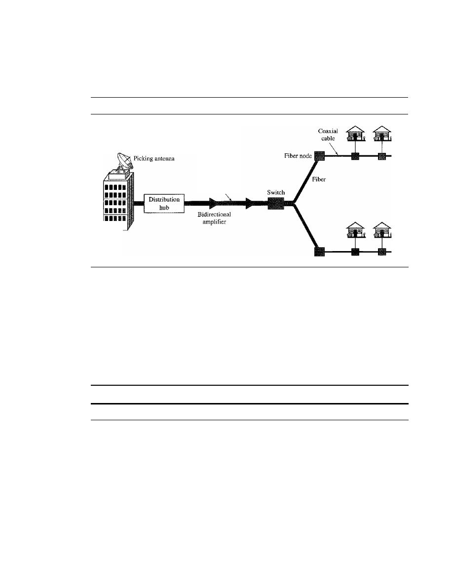
SECTION
9.5
CABLE TV FOR DATA TRANSFER
257
medium from the cable TV office to a box, called the fiber node, is optical fiber; from the
fiber node through the neighborhood and into the house is still coaxial cable. Figure 9.15
shows a schematic diagram of an HFC network.
Figure
9.15
Hybridfiber-coaxial (HFC) network
RCH
High-bandwidth
fiber
The regional cable head (RCH) normally serves up to 400,000 subscribers. The
RCHs feed the distribution hubs, each of which serves up to 40,000 subscribers. The
distribution hub plays an important role in the new infrastructure. Modulation and dis-
tribution of signals are done here; the signals are then fed to the fiber nodes through
fiber-optic cables. The fiber node splits the analog signals so that the same signal is sent
to each coaxial cable. Each coaxial cable serves up to 1000 subscribers. The use of
fiber-optic cable reduces the need for amplifiers down to eight or less.
One reason for moving from traditional to hybrid infrastructure is to make the cable
network bidirectional (two-way).
Communication in an HFC cable TV network can be bidirectional.
9.5
CABLE TV
FOR
DATA TRANSFER
Cable companies are now competing with telephone companies for the residential
customer who wants high-speed data transfer. DSL technology provides high-data-rate
connections for residential subscribers over the local loop. However, DSL uses the
existing unshielded twisted-pair cable, which is very susceptible to interference. This
imposes an upper limit on the data rate. Another solution is the use of the cable TV net-
work. In this section, we briefly discuss this technology.
Bandwidth
Even in an HFC system, the last part of the network, from the fiber node to the sub-
scriber premises, is still a coaxial cable. This coaxial cable has a bandwidth that ranges
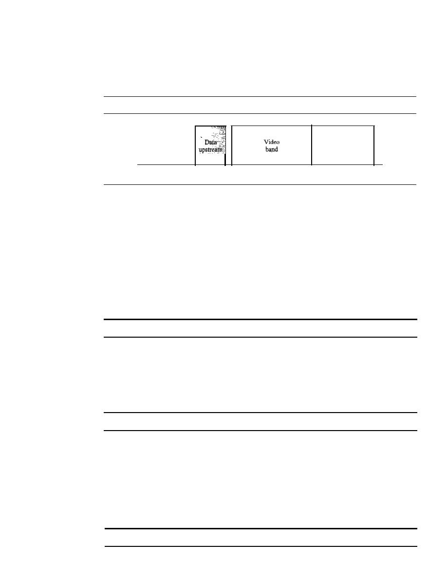
258
CHAPTER
9
USING TELEPHONE AND CABLE NETWORKS FOR DATA TRANSMISSION
from 5 to 750 MHz (approximately). To provide Internet access, the cable company has
divided this bandwidth into three bands: video, downstream data, and upstream data, as
shown in Figure 9.16.
Figure 9.16
Division of coaxial cable band
by
CATV
Frequency, MHz
5
4254
550
Data
downstream
750
Downstream Video Band
The
downstream video band
occupies frequencies from 54 to 550 MHz. Since each
TV channel occupies 6 MHz, this can accommodate more than 80 channels.
Downstream Data Band
The downstream data (from the Internet to the subscriber premises) occupies the upper
band, from 550 to 750 MHz. This band is also divided into 6-MHz channels.
Modulation
Downstream data band
uses the 64-QAM (or possibly 256-QAM)
modulation technique.
Downstream data are modulated using the 64-QAM modulation technique.
Data Rate
There is 6 bits/baud
in
64-QAM. One bit is used for forward error correction;
this leaves 5 bits of data per baud. The standard specifies I Hz for each baud; this means that,
theoretically, downstream data can be received at 30 Mbps (5 bitslHz
x
6 MHz). The stan-
dard specifies only 27 Mbps. However, since the cable modem is normally connected to the
computer through a lOBase-T cable (see Chapter 13), this limits the data rate to 10 Mbps.
The theoretical downstream data rate is 30 Mbps.
Upstream Data Band
The upstream data (from the subscriber premises to the Internet) occupies the lower
band, from 5 to 42 MHz. This band is also divided into 6-MHz channels.
Modulation
The
upstream data band
uses lower frequencies that are more suscepti-
ble to noise and interference. For this reason, the QAM technique is not suitable for this
band. A better solution is QPSK.
Upstream data are modulated using the QPSK modulation technique.

SECTION
9.5
CABLE TV FOR DATA TRANSFER
259
Data Rate
There are
2
bitslbaud in QPSK. The standard specifies
1
Hz for each baud;
this means that, theoretically, upstream data can be sent at 12 Mbps (2 bitslHz x 6 MHz).
However, the data rate is usually less than 12 Mbps.
The theoretical upstream data rate is 12 Mbps.
Sharing
Both upstream and downstream bands are shared by the subscribers.
Upstream Sharing
The upstream data bandwidth is 37 MHz. This means that there are only six 6-MHz
channels available in the upstream direction. A subscriber needs to use one channel to
send data in the upstream direction. The question is, "How can six channels be shared in
an area with 1000,2000, or even 100,000 subscribers?" The solution is timesharing. The
band is divided into channels using FDM; these channels must be shared between sub-
scribers in the same neighborhood. The cable provider allocates one channel, statically
or dynamically, for a group of subscribers. If one subscriber wants to send data, she or
he contends for the channel with others who want access; the subscriber must wait until
the channel is available.
Downstream Sharing
We have a similar situation in the downstream direction. The downstream band has
33 channels of 6 MHz. A cable provider probably has more than 33 subscribers; therefore,
each channel must be shared between a group of subscribers. However, the situation is dif-
ferent for the downstream direction; here we have a multicasting situation.
If
there are data
for any of the subscribers in the group, the data are sent to that channel. Each subscriber is
sent the data. But since each subscriber also has an address registered with the provider; the
cable modem for the group matches the address carried with the data to the address assigned
by the provider. If the address matches, the data are kept; otherwise, they are discarded.
CMandCMTS
To use a cable network for data transmission, we need two key devices: a
cable modem
(CM)
and a
cable modem transmission system (CMTS).
CM
The
cable modem (CM)
is installed on the subscriber premises. It is similar
to
an ADSL
modem. Figure 9.17 shows its location.
CMTS
The
cable modem transmission system (CMTS)
is installed inside the distribution
hub by the cable company.
It
receives data from the Internet and passes them to the
combiner, which sends them to the subscriber. The CMTS also receives data from the
subscriber and passes them to the Internet. Figure 9.18 shows the location of the CMTS.
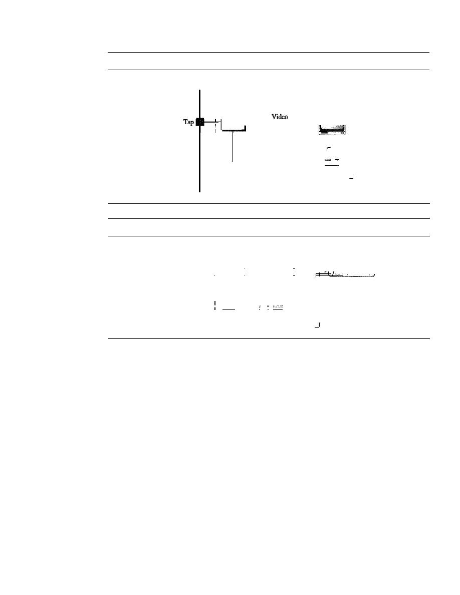
260
CHAPTER
9
USING TELEPHONE AND CABLE NETWORKS FOR DATA TRANSMISSION
Figure 9.17
Cable modem (CM)
Cable
Customer residence
r - - - - - - - - - - - - - - - - - - - - - - - - I
I
I
I
I
I
I
1
1
1
1
Data
1
1
1
1
Cable modem
1
1
Figure 9.18
Cable modem transmission system (CMTS)
From head end
To and from
the Internet
Distribution hub
-------------------
I
I
Video
I
I
Fiber
I
I
Combiner
I
I
I
I
I
I
I
I
I
Data
:
I
I
I
CMTS
I
L
Data Transmission Schemes: DOeSIS
During the last few decades, several schemes have been designed to create a standard for
data transmission over an HFC network. Prevalent is the one devised by Multimedia
Cable Network Systems (MCNS), called Data Over Cable System Interface Specifi-
cation (DOCSIS). DOCSIS defines all the protocols necessary to transport data from a
CMTS to aCM.
Upstream Communication
The following is a very simplified version of the protocol defined by DOCSIS for
upstream communication.
It
describes the steps that must be followed by a CM:
1. The CM checks the downstream channels for a specific packet periodically sent by
the CMTS. The packet asks any new CM to announce itself on a specific upstream
channel.
2. The CMTS sends a packet to the CM, defining its allocated downstream and
upstream channels.
3. The CM then starts a process, called ranging, which determines the distance
between the CM and CMTS. This process is required for synchronization between all

SECTION
9. 7
KEY TERMS
261
CMs and CMTSs for the minislots used for timesharing of the upstream channels.
We will learn about this timesharing when we discuss contention protocols in
Chapter 12.
4. The CM sends a packet to the ISP, asking for the Internet address.
5. The CM and CMTS then exchange some packets to establish security parameters,
which are needed for a public network such as cable TV.
6. The CM sends its unique identifier to the CMTS.
7. Upstream communication can start in the allocated upstream channel; the CM can
contend for the minislots to send data.
Downstream Communication
In the downstream direction, the communication is much simpler. There is no conten-
tion because there is only one sender. The CMTS sends the packet with the address of
the receiving eM, using the allocated downstream channel.
9.6
RECOMMENDED READING
For more details about subjects discussed in this chapter, we recommend the following
books. The items in brackets [...] refer to the reference list at the end of the text.
Books
[CouOl] gives an interesting discussion about telephone systems, DSL technology,
and CATV in Chapter 8. [Tan03] discusses telephone systems and DSL technology in
Section 2.5 and CATV in Section 2.7. [GW04] discusses telephone systems in Sec-
tion 1.1.1 and standard modems in Section 3.7.3. A complete coverage of residential
broadband (DSL and CATV) can be found in [Max99].
9.7
KEY TERMS
56Kmodem
800 service
900 service
ADSL Lite
ADSLmodem
analog leased service
analog switched service
asymmetric DSL (ADSL)
cable modem (CM)
cable modem transmission system
(CMTS)
cable TV network
common carrier
community antenna TV (CATV)
competitive local exchange carrier
(CLEC)
Data Over Cable System Interface
Specification (DOCSIS)
demodulator
digital data service (DDS)
digital service
digital subscriber line (DSL)
digital subscriber line access multiplexer
(DSLAM)
discrete multitone technique (DMT)
distribution hub

262
CHAPTER
9
USING TELEPHONE AND CABLE NETWORKS FOR DATA TRANSMISSION
downloading
downstream data band
end office
fiber node
head end
high-bit-rate DSL (HDSL)
hybrid fiber-coaxial (HFC) network
in-band signaling
incumbent local exchange carrier
(ILEC)
interexchange carrier (IXC)
ISDN user port (ISUP)
local access transport area (LATA)
local exchange carrier (LEC)
local loop
long distance company
message transport port (MTP) level
modem
modulator
out-of-band signaling
plain old telephone system (POTS)
point of presence (POP)
ranging
regional cable head (RCH)
regional office
server control point (SCP)
signal point (SP)
signal transport port (STP)
signaling connection control point
(SCep)
Signaling System Seven (SS7)
switched/56 service
switching office
symmetric DSL (SDSL)
tandem office
telephone user port (TUP)
transaction capabilities application port
(TCAP)
trunk
uploading
upstream data band
Y.32
Y.32bis
Y.34bis
Y.90
Y.92
very-high-bit-rate DSL (VDSL)
video band
V-series
wide-area telephone service (WATS)
9.8
SUMMARY
o
The telephone, which is referred to as the plain old telephone system (POTS),
was originally an analog system. During the last decade, the telephone network
has undergone many technical changes. The network is now digital as well as
analog.
o
The telephone network is made of three major components: local loops, trunks,
and switching offices. It has several levels of switching offices such as end offices,
tandem offices, and regional offices.
o
The United States is divided into many local access transport areas (LATAs). The
services offered inside a LATA are called intra-LATA services. The carrier that
handles these services is called a local exchange carrier (LEC). The services
between LATAs are handled by interexchange carriers (lXCs).
o
In in-band signaling, the same circuit is used for both signaling and data. In out-of-
band signaling, a portion of the bandwidth is used for signaling and another portion

SECTION
9.9
PRACTICE SET
263
for data. The protocol that is used for signaling in the telephone network is called
Signaling System Seven (SS7).
o
Telephone companies provide two types of services: analog and digital. We can
categorize analog services as either analog switched services or analog leased ser-
vices. The two most common digital services are switched/56 service and digital
data service (DDS).
o
Data transfer using the telephone local loop was traditionally done using a dial-up
modem. The term
modem
is a composite word that refers to the two functional
entities that make up the device: a signal modulator and a signal demodulator.
o
Most popular modems available are based on the V-series standards. The V.32 modem
has a data rate of 9600 bps. The V32bis modem supports 14,400-bps transmission.
V90 modems, called 56K modems, with a downloading rate of 56 kbps and upload-
ing rate of 33.6 kbps are very common. The standard above V90 is called V92. These
modems can adjust their speed, and if the noise allows, they can upload data at the rate
of 48 kbps.
o
Telephone companies developed another technology, digital subscriber line (DSL), to
provide higher-speed access to the Internet. DSL technology is a set of technologies,
each differing in the first letter (ADSL, VDSL, HDSL, and SDSL. ADSL provides
higher speed in the downstream direction than in the upstream direction. The high-bit-
rate digital subscriber line (HDSL) was designed as an alternative to the T-l line
(1.544 Mbps). The symmetric digital subscriber line (SDSL) is a one twisted-pair ver-
sion of HDSL. The very high-bit-rate digital subscriber line (VDSL) is an alternative
approach that is similar to ADSL.
o
Community antenna TV (CATV) was originally designed to provide video services
for the community. The traditional cable TV system used coaxial cable end to end.
The second generation of cable networks is called a hybrid fiber-coaxial (HFC)
network. The network uses a combination of fiber-optic and coaxial cable.
o
Cable companies are now competing with telephone companies for the residential
customer who wants high-speed access to the Internet. To use a cable network for
data transmission, we need two key devices: a cable modem (CM) and a cable modem
transmission system (CMTS).
9.9
PRACTICE SET
Review Questions
1. What are the three major components of a telephone network?
2. Give some hierarchical switching levels of a telephone network.
3. What is LATA? What are intra-LATA and inter-LATA services?
4. Describe the SS7 service and its relation to the telephone network.
S.
What are the two major services provided by telephone companies in the United
States?
6. What is dial-up modem technology? List some of the common modem standards
discussed in this chapter and give their data rates.

264
CHAPTER
9
USING TELEPHONE AND CABLE NETWORKS FOR DATA TRANSMISSION
7. What is DSL technology? What are the services provided by the telephone companies
using DSL? Distinguish between a DSL modem and a DSLAM.
8. Compare and contrast a traditional cable network with a hybrid fiber-coaxial network.
9. How is data transfer achieved using CATV channels?
10. Distinguish between CM and CMTS.
Exercises
11. Using the discussion of circuit-switching in Chapter 8, explain why this type of
switching was chosen for telephone networks.
12. In Chapter 8, we discussed the three communication phases involved in a circuit-
switched network. Match these phases with the phases in a telephone call between
two parties.
13.
In
Chapter 8, we learned that a circuit-switched network needs end-to-end addressing
during the setup and teardown phases. Define end-to-end addressing in a telephone
network when two parties communicate.
14. When we have an overseas telephone conversation, we sometimes experience a
delay. Can you explain the reason?
15. Draw a barchart to compare the different downloading data rates of common modems.
16. Draw a barchart to compare the different downloading data rates of common DSL
technology implementations (use minimum data rates).
17. Calculate the minimum time required to download one million bytes of information
using each of the following technologies:
a. V32 modem
b. V32bis modem
c. V90 modem
18. Repeat Exercise 17 using different DSL implementations (consider the minimum
rates).
19. Repeat Exercise 17 using a cable modem (consider the minimum rates).
20. What type of topology is used when customers in an area use DSL modems for
data transfer purposes? Explain.
21. What type of topology
used when customers in an area use cable modems for
data transfer purposes? Explain.
Data Link
Layer
Objectives
The data link layer transforms the physical layer, a raw transmission facility, to a link
responsible for node-to-node (hop-to-hop) communication. Specific responsibilities of
the data link layer include framing, addressing, flow control, error control, and media
access control.
The data link layer divides the stream of bits received from the network
layer into manageable data units called frames. The data link layer adds a header to the
frame to define the addresses of the sender and receiver of the frame.
If
the rate at
which the data are absorbed by the receiver is less than the rate at which data are pro-
duced in the sender, the data link layer imposes a flow control mechanism to avoid
overwhelming the receiver. The data link layer also adds reliability to the physical layer
by adding mechanisms to detect and retransmit damaged, duplicate, or lost frames.
When two or more devices are connected to the same link, data link layer protocols are
necessary to determine which device has control over the link at any given time.
In Part 3 of the book, we first discuss services provided by the data link layer. We
then discuss the implementation of these services in local area networks (LANs). Finally
we discuss how wide area networks (WANs) use these services.
Part 3 of the book is devoted to the data link layer and
the services provided by this layer.
Chapters
This part consists of nine chapters: Chapters 10 to 18.
Chapter 10
Chapter 10 discusses error detection and correction. Although the quality of devices and
media have been improved during the last decade, we still need to check for errors and
correct them in most applications.

Chapter 11
Chapter 11 is named data link control, which involves flow and error control.
It
dis-
cusses some protocols that are designed to handle the services required from the data
link layer in relation to the network layer.
Chapter 12
Chapter 12 is devoted to access control, the duties of the data link layer that are related
to the use of the physical layer.
Chapter 13
This chapter introduces wired local area networks. A wired LAN, viewed as a link, is
mostly involved in the physical and data link layers. We have devoted the chapter to the
discussion of Ethernet and its evolution, a dominant technology today.
Chapter 14
This chapter introduces wireless local area networks. The wireless LAN is a growing
technology in the Internet. We devote one chapter to this topic.
Chapter 15
After discussing wired and wireless LANs, we show how they can be connected together
using connecting devices.
Chapter 16
This is the first chapter on wide area networks (WANs). We start with wireless WANs
and then move on to satellite networks and mobile telephone networks.
Chapter 17
To demonstrate the operation of a high-speed wide area network that can be used as a
backbone for other WANs or for the Internet, we have chosen to devote all of Chapter 17
to SONET, a wide area network that uses fiber-optic technology.
Chapter 18
This chapter concludes our discussion on wide area networks. Two switched WANs,
Frame Relay and ATM, are discussed here.

CHAPTER 10
Error Detection and Correction
Networks must be able to transfer data from one device to another with acceptable accu-
racy. For most applications, a system must guarantee that the data received are identical to
the data transmitted. Any time data are transmitted from one node to the next, they can
become corrupted in passage. Many factors can alter one or more bits of a message. Some
applications require a mechanism for detecting and correcting
errors.
Data can be corrupted during transmission.
Some applications require that errors be detected and corrected.
Some applications can tolerate a small level of error. For example, random errors
in audio or video transmissions may be tolerable, but when we transfer text, we expect
a very high level of accuracy.
10.1
INTRODUCTION
Let us first discuss some issues related, directly or indirectly, to error detection and
correcion.
Types
of Errors
Whenever bits flow from one point to another, they are subject to unpredictable
changes because of
interference.
This interference can change the shape of the signal.
In a single-bit error, a 0 is changed to a 1 or a 1 to a O. In a burst error, multiple bits are
changed. For example, a 11100 s burst of impulse noise on a transmission with a data
rate of 1200 bps might change all or some of the 12 bits of information.
Single-Bit Error
The term
single-bit error
means that only 1 bit of a given data unit (such as a byte,
character, or packet) is changed from 1 to 0 or from 0 to 1.
267
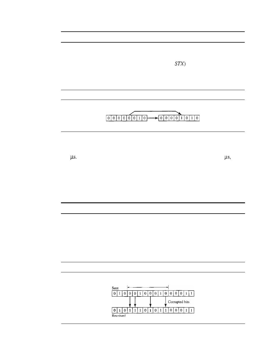
268
CHAPTER 10
ERROR DETECTION AND CORRECTION
In
a single-bit error, only 1 bit in the data unit has changed.
Figure
10.1
shows the effect of a single-bit error on a data unit. To understand the
impact of the change, imagine that each group of 8 bits is an ASCII character with a 0 bit
added to the left. In Figure
10.1,00000010
(ASCII
was sent, meaning
start of
text,
but
00001010
(ASCII
LF)
was received, meaning
line feed.
(For more information
about ASCII code, see Appendix A.)
:Figure
10.1
Single-bit error
o
changed to
I
Sent
Received
Single-bit errors are the least likely type of error in serial data transmission. To under-
stand why, imagine data sent at
1
Mbps. This means that each bit lasts only
1/1,000,000
s,
or
1
For a single-bit error to occur, the noise must have a duration of only
1
which
is very rare; noise normally lasts much longer than this.
Burst Error
The term
burst error
means that
2
or more bits in the data unit have changed from
1
to
0
or from
0
to
1.
A burst error means that 2 or more bits in the data unit have changed.
Figure
10.2
shows the effect of a burst error on a data unit. In this case,
0100010001000011
was sent, but
0101110101100011
was received. Note that a burst
error does not necessarily mean that the errors occur in consecutive bits. The length of
the burst is measured from the first corrupted bit to the last corrupted bit. Some bits in
between may not have been corrupted.
Figure
10.2
Burst error of length 8
Length of burst
error (8 bits)

SECTION 10.1
INTRODUCTION
269
A burst error
more likely to occur than a single-bit error. The duration of noise is
normally longer than the duration of 1 bit, which means that when noise affects data, it
affects a set of bits. The number of bits affected depends on the data rate and duration
of noise. For example, if we are sending data at I kbps, a noise of 11100 s can affect
10 bits; if we are sending data at I Mbps, the same noise can affect 10,000 bits.
Redundancy
The central concept in detecting or correcting errors is redundancy. To be able to
detect or correct errors, we need to send some extra bits with our data. These redundant
bits are added by the sender and removed by the receiver. Their presence allows the
receiver to detect or correct corrupted bits.
To detect or correct errors, we need to send
(redundant) bits with data.
Detection Versus Correction
The correction of errors is more difficult than the detection. In error detection, we are
looking only to see if any error has occurred. The answer is a simple yes or no. We are
not even interested in the number of errors. A single-bit error is the same for us as a
burst error.
In error correction, we need to know the exact number of bits that are corrupted and
more importantly, their location
the message. The number of the errors and the size of
the message are important factors.
If
we need to correct one single error
an 8-bit data
unit, we need to consider eight possible error locations; if we need to correct two errors
in a data unit of the same size, we need to consider 28 possibilities. You can imagine the
receiver's difficulty in finding 10 errors in a data unit of 1000 bits.
Forward Error Correction Versus Retransmission
There are two main methods of error correction. Forward error correction
the pro-
cess in which the receiver tries to guess the message by using redundant bits. This
possible, as we see later, if the number of errors
small. Correction by retransmission
a technique in which the receiver detects the occurrence of an error and asks the sender
to resend the message. Resending is repeated until a message arrives that the receiver
believes is error-free (usually, not all errors can be detected).
Coding
Redundancy is achieved through various coding schemes. The sender adds redundant
bits through a process that creates a relationship between the redundant bits and the
actual data bits. The receiver checks the relationships between the two sets of bits to
detect or correct the errors. The ratio of redundant bits to the data bits and the robust-
ness of the process are important factors
any coding scheme. Figure 10.3 shows the
general idea of coding.
We can divide coding schemes into two broad categories: block coding and convo-
lution coding. In this book, we concentrate on block coding; convolution coding is
more complex and beyond the scope of this book.
270
CHAPTER 10
ERROR DETECTION AND CORRECTION
Figure 10.3
The structure ofencoder and decoder
Sender
Receiver
Encoder
Decoder
I
Message
I
t
correct or
discard
Generator
I
I
Checker
I
t
In this book, we concentrate on block codes; we leave convolution codes to advanced texts.
Modular Arithmetic
Before we finish this section, let us briefly discuss a concept basic to computer science
in general and to error detection and correction in particular: modular arithmetic. Our
intent here is not to delve deeply into the mathematics of this topic; we present just
enough information to provide a background to materials discussed in this chapter.
In
modular arithmetic,
we use only a limited range of integers. We define
an
upper
limit, called a
modulus
N.
We then use only the integers
0
to
N -
I, inclusive. This is
modulo-N
arithmetic. For example, if the modulus is 12, we use only the integers
0
to
11, inclusive. An example of modulo arithmetic is our clock system. It is based on
modulo-12 arithmetic, substituting the number 12 for
O.
In a
modulo-N
system, if a
number is greater than
N,
it is divided by
N
and the remainder is the result.
If
it is neg-
ative, as many
Ns
as needed are added to make it positive. Consider our clock system
again. If we start a job at 11
A.M.
and the job takes
5
h, we can say that the job is to be
finished at 16:00 if we are in the military, or we can say that it will be finished at
4
P.M.
(the remainder of 16/12 is
4).
In modulo-N arithmetic, we use only the integers in the range 0 to
N
1, inclusive.
Addition and subtraction in modulo arithmetic are simple. There is no carry when
you add two digits in a column. There is no carry when you subtract one digit from
another in a column.
Modulo-2 Arithmetic
Of particular interest is modulo-2 arithmetic. In this arithmetic, the modulus
N
is
2.
We
can use only 0 and 1. Operations in this arithmetic are very simple. The following
shows how we can add or subtract 2 bits.
Adding:
Subtracting:
0+0=0
0-0=0
0+1=1
0-1=1
1+0=1
1+1=0
1-1=0
SECTION 10.2
BLOCK CODING
271
Notice particularly that addition and subtraction give the same results. In this arith-
metic we use the XOR (exclusive OR) operation for both addition and subtraction. The
result of an XOR operation is 0 if two bits are the same; the result is I if two bits are
different. Figure 10.4 shows this operation.
Figure 10.4
XORing of two single bits or two words
a. Two
bits
are the same, the result is
O.
b.
Two
bits
are different, the result is
1.
o
o
I
I
0
I
0
°
°
°
°
c. Result of XORing two patterns
Other Modulo Arithmetic
We also use, modulo-N arithmetic through the book. The principle is the same; we use
numbers between 0 and
N -
1.
If
the modulus is not 2, addition and subtraction are distinct.
If we get a negative result, we add enough multiples of
N
to make it positive.
10.2
BLOCK CODING
In block coding, we divide our message into blocks, each of k bits, called datawords. We
add r redundant bits to each block to make the length n
=
k
+
r.
The resulting n-bit blocks
are called codewords. How the extra
r
bits is chosen or calculated is something we will
discuss later. For the moment, it is important to know that we have a set of datawords,
each of size
k,
and a set of codewords, each of size of n. With
k
bits, we can create a com-
bination of
2
k
datawords; with n bits, we can create a combination of
2
n
codewords.
Since
n
>
k,
the number of possible codewords is larger than the number of possible data-
words. The block coding process is one-to-one; the same dataword is always encoded as
the same codeword. This means that we have
2
n
-
2
k
codewords that are not used. We
call these codewords invalid or illegal. Figure 10.5 shows the situation.
Figure 10.5
Datawords and codewords in block coding
II
Hits
II
Hits
I •
eo
I
Hits
I
I
2
k
Datawords, each of
k
bits
II
bits
II
bits
nbits
II
2
n
Codewords, each of
n bits (only
2
k
of them are valid)
272
CHAPTER
10
ERROR DETECTION AND CORRECTION
Example 10.1
The 4B/5B block coding discussed in Chapter 4 is a good example of this type of coding. In this
coding scheme,
k
=
4 and n
=
5. As we saw, we have
2
k
=
16 datawords and
2
n
=
32 codewords.
We saw that 16 out of 32 codewords are used for message transfer and the rest are either used for
other purposes or unused.
Error Detection
How can errors be detected by using block coding?
If
the following two conditions are
met, the receiver can detect a change in the original codeword.
1. The receiver has (or can find) a list of valid codewords.
2. The original codeword has changed to an invalid one.
Figure 10.6 shows the role of block coding in error detection.
Figure 10.6
Process of error detection in block coding
Sender
Receiver
Encoder
Decoder
k
bits
I
I
k
bits
I
t
Extract
I
Generator
I
I
Checker
Discard
i
n bits
I
Unreliable transmission
I
n bits
I
The sender creates codewords out of datawords by using a generator that applies the
rules and procedures of encoding (discussed later). Each codeword sent to the receiver may
change during transmission.
If
the received codeword is the same as one of the valid code-
words, the word is accepted; the corresponding dataword is extracted for use. If the received
codeword is not valid, it is discarded. However, if the codeword is corrupted during trans-
mission but the received word still matches a valid codeword, the error remains undetected.
This type of coding can detect only single errors. Two or more errors may remain undetected.
Example 10.2
Let us assume that
k
=
2 and n
=
3. Table 10.1 shows the list of datawords and codewords. Later,
we will see how to derive a codeword from a dataword.
Table 10.1
A code for error detection (Example 10.2)
Datawords
Codewords
00
000
01
011
10
101
11
110
SECTION 10.2
BLOCK CODING
273
Assume the sender encodes the dataword 01 as 011 and sends it to the receiver. Consider the
following cases:
1.
The receiver receives OIl. It is a valid codeword. The receiver extracts the dataword 01
from it.
2. The codeword is corrupted during transmission, and 111 is received (the leftmost bit is cor-
rupted). This is not a valid codeword and is discarded.
The codeword is corrupted during transmission, and 000 is received (the right two bits are
corrupted). This is a valid codeword. The receiver incorrectly extracts the dataword 00. Two
corrupted bits have made the error undetectable.
An error-detecting code can detect only the types of errors for which it is designed;
other types of errors may remain undetected.
Error Correction
As we said before, error correction
much more difficult than error detection. In error
detection, the receiver needs to know only that the received codeword is invalid; in
error correction the receiver needs to find (or guess) the original codeword sent. We can
say that we need more redundant bits for error correction than for error detection.
Figure 10.7 shows the role of block coding
error correction. We can see that the idea
is the same as error detection but the checker functions are much more complex.
Figure 10.7
Structure of encoder and decoder in error correction
Sender
Receiver
Encoder
Decoder
k bits
I
Dataword
I
I
Dataword
I
k bits
I
t
Correct
I
Generator
I
I
Checker
I
i
n bits
I
I
Unreliable transmission
I
n bits
Codeword
I
I
Codeword
Example 10.3
Let us add more redundant bits to Example 10.2 to see if the receiver can correct an error without
knowing what was actually sent. We add 3 redundant bits to the 2-bit dataword to make 5-bit
codewords. Again, later we will show how we chose the redundant bits. For the moment let us
concentrate on the error correction concept. Table 10.2 shows the datawords and codewords.
Assume the dataword is 01. The sender consults the table (or uses an algorithm) to create the
codeword 01011. The codeword is corrupted during transmission, and 01001 is received (error in
the second bit from the right). First, the receiver finds that the received codeword is not in the table.
This means an error has occurred. (Detection must come before correction.) The receiver, assuming
that there is only 1 bit corrupted, uses the following strategy to guess the correct dataword.

274
CHAPTER 10
ERROR DETECTION AND CORRECTION
Table 10.2
A code for error correction (Example 10.3)
Dataword
Codeword
00
00000
01
01011
10
10101
11
11110
I. Comparing the received codeword with the first codeword in the table (01001 versus 00000),
the receiver decides that the first codeword is not the one that was sent because there are two
different bits.
2. By the same reasoning, the original codeword cannot be the third or fourth one in the table.
3. The original codeword must be the second one in the table because this is the only one that
differs from the received codeword by 1 bit. The receiver replaces 01001 with 01011 and
consults the table to find the dataword 01.
Hamming Distance
One of the central concepts in coding for error control is the idea of the Hamming dis-
tance. The Hamming distance between two words (of the same size) is the number of
differences between the corresponding bits. We show the Hamming distance between
two words
x
and
y
as
d(x,
y).
The Hamming distance can easily be found if wc apply the XOR operation
on the
two words and count the number of Is in the result. Note that the Hamming distance is
a value greater than zero.
The Hamming distance between two words is the number
of differences between corresponding bits.
Example 10.4
Let us find the Hamming distance between two pairs of words.
1. The Hamming distance
d(OOO,
011) is 2 because 000
011 is 011 (two Is).
2. The Hamming distance
d(10101,
11110) is 3 because 10101
11110 is 01011 (three Is).
Minimum Hamming Distance
Although the concept of the Hamming distance is the central point in dealing with error
detection and correction codes, the measurement that is used for designing a code is the
minimum Hamming distance. In a set of words, the minimum Hamming distance is the
smallest Hamming distance between all possible pairs. We use d
min
to define the mini-
mum Hamming distance in a coding scheme. To find this value, we find the Hamming
distances between all words and select the smallest one.
The minimum Hamming distance is the smallest Hamming
distance between all possible pairs in a set of words.

SECTION iO.2
BLOCK CODiNG
275
Example 10.5
Find the minimum Hamming distance of the coding scheme in Table 10.1.
Solution
We first find all Hamming distances.
d(OOO,
011)
=
2
d(Oll,110)=2
The
d
min
in this case is 2.
d(OOO,
101)
=
2
d(W1,
110)
=
2
d(OaO,
110)
=
2
d(Oll,
101)
=
2
Example 10.6
Find the minimum Hamming distance of the coding scheme in Table 10.2.
Solution
We first find all the Hamming distances.
d(OOOOO,
01011)
=
3
d(01011,
10101)
=
4
The
d
min
in this case is 3.
d(OOOOO,
10101)
=
3
d(OlO11,
11110)
=
3
d(OOOOO,
11110)
4
d(10101, 11110)
=
3
Three Parameters
Before we continue with our discussion, we need to mention that any coding scheme
needs to have at least three parameters: the codeword size
n, the dataword size
k,
and
the minimum Hamming distance
d
min.
A coding scheme C is written as
C(n, k)
with a
separate expression for
For example, we can call our first coding scheme
C(3, 2)
with d
min
=
2 and our second coding scheme
C(5,
2) with d
min
3.
Hamming Distance and Error
Before we explore the criteria for error detection or correction, let us discuss the relationship
between the Hamming distance and errors occurring during transmission. When a codeword
is corrupted during transmission, the
distance between the sent and received code-
words is the number of bits affected by the error. In other words, the Hamming distance
between the received codeword and the sent codeword is the number of bits that are corrupted
during transmission. For example, if the codeword 00000 is sent and 01101 is received, 3 bits
are in error and the Hamming distance between the two is
d(OOOOO,
01101)
=
3.
Minimum Distance for Error Detection
Now let us find the minimum Hamming distance in a code if we want to be able to detect
up to s errors.
If
s errors occur during transmission, the Hamming distance between the
sent codeword and received codeword is s. If our code is to detect up to s errors, the mini-
mum distance between the valid codes must be s
+
1, so that the received codeword does
not match a valid codeword. In other words, if the minimum distance between all valid
codewords is s
+
1, the received codeword cannot be erroneously mistaken for another
codeword. The distances are not enough (s
+
1) for the receiver to accept it as valid. The
error will be detected. We need to clarify a point here: Although a code with
dmin
=
s
+
1
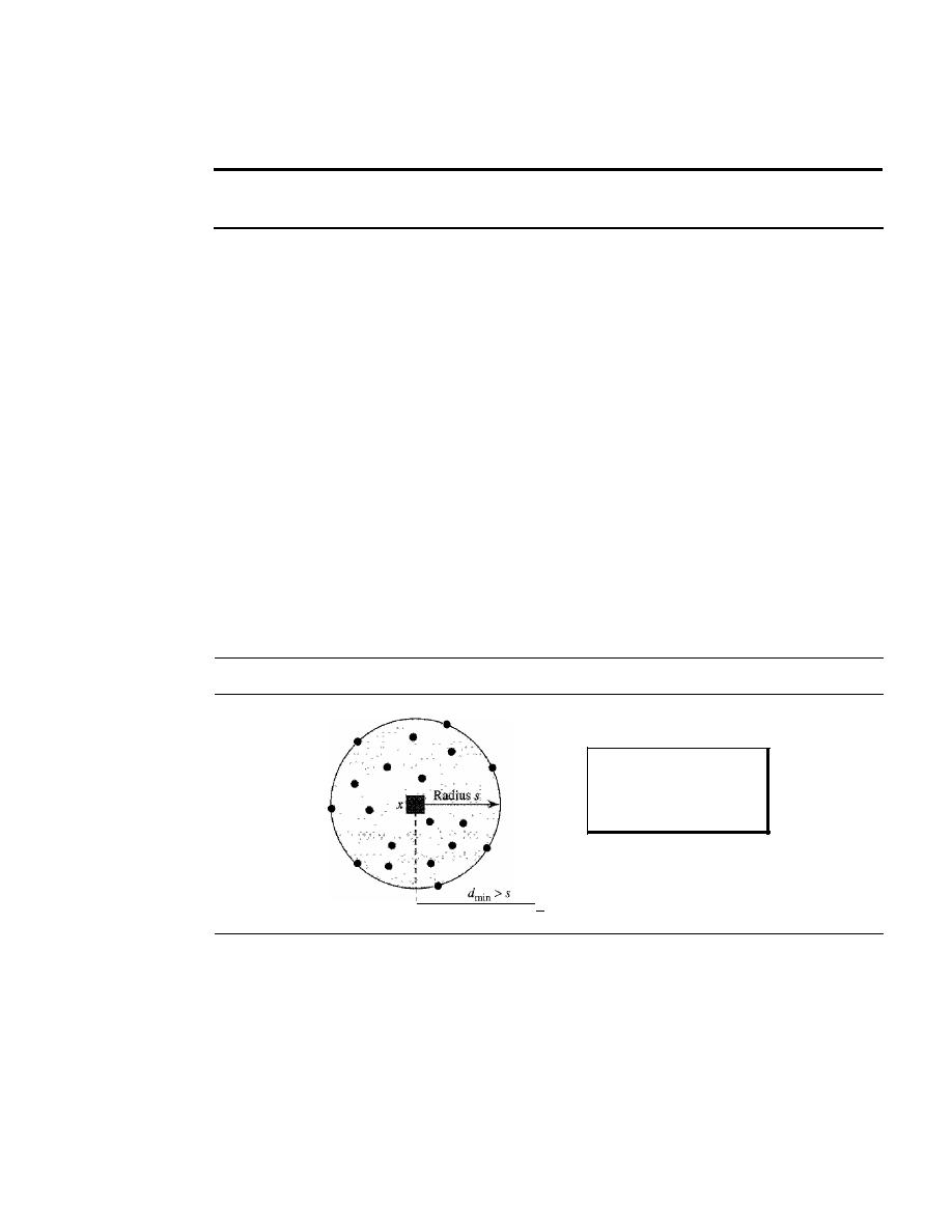
276
CHAPTER 10
ERROR DETECTION AND CORRECTION
may be able to detect more than s errors in some special cases, only s or fewer errors are
guaranteed to be detected.
To guarantee the detection of up to
s
errors in all cases, the minimum
Hamming distance in a block code must be d
min
=
S
+
1.
Example 10.7
The minimum Hamming distance for our first code scheme (Table 10.1) is 2. This code guarantees
detection of only a single error. For example, if the third codeword (l0
1)
is sent and one error
occurs, the received codeword does not match any valid codeword.
If
two errors occur, however,
the received codeword may match a valid codeword and the errors are not detected.
Example 10.8
Our second block code scheme (Table 10.2) has
d
min
=
3. This code can detect up to two errors.
Again, we see that when any of the valid codewords is sent, two errors create a codeword which
is not in the table of valid codewords. The receiver cannot be fooled. However, some combina-
tions of three errors change a valid codeword to another valid codeword. The receiver accepts the
received codeword and the errors are undetected.
We can look at this geometrically. Let us assume that the sent codeword
x
is at the
center of a circle with radius
s.
All other received codewords that are created by 1 to
s
errors are points inside the circle or on the perimeter of the circle. All other valid code-
words must be outside the circle, as shown in Figure 10.8.
Figure 10.8
Geometric concept for finding d
min
in error detection
.y
I
I
I
I
I
I
I
I
I
'1
Legend
•
Any valid codeword
•
Any corrupted codeword
with 0 to s errors
In Figure 10.8, d
min
must be an integer greater than
s;
that is, d
min
=
s
+
1.
Minimum Distance for Error Correction
Error correction is more complex than error detection; a decision is involved. When a
received codeword is not a valid codeword, the receiver needs to decide which valid
codeword was actually sent. The decision is based on the concept of territory, an exclu-
sive area surrounding the codeword. Each valid codeword has its own territory.
We use a geometric approach to define each territory. We assume that each valid
codeword has a circular territory with a radius of
t
and that the valid codeword is at the
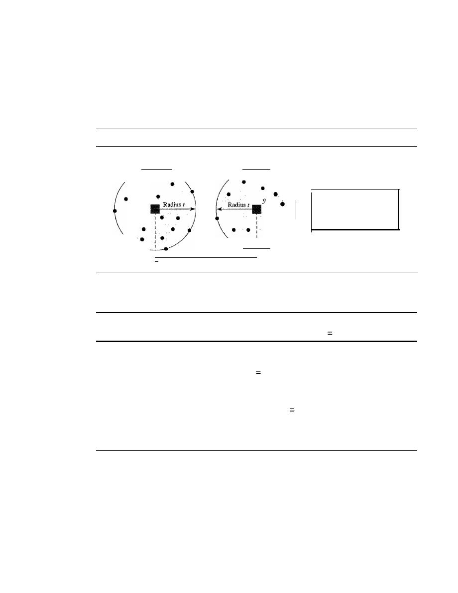
SECTION 10.3
LINEAR BLOCK CODES
277
center. For example, suppose a codeword
x
is corrupted by
t
bits or less. Then this cor-
rupted codeword is located either inside or on the perimeter of this circle.
If
the receiver
receives a codeword that belongs to this territory, it decides that the original codeword is
the one at the center. Note that we assume that only up to
t
errors have occurred; other-
wise, the decision is wrong. Figure 10.9 shows this geometric interpretation. Some texts
use a sphere to show the distance between all valid block codes.
Figure 10.9
Geometric concept for finding d
min
in error correction
•
Territory of
x
•
e
x
I '
d
min
>
2t
Territory of
y
Legend
:
•
Any valid codeword
•
•
•
Any corrupted codeword
with 1 to terrors
• •
In Figure 10.9,
d
min
>
2t;
since the next integer increment is 1, we can say that
d
min
=
2t
+
1.
To guarantee correction of up to
t
errors in all cases, the minimum
Hamming distance in a block code must be d
min
2t
+
1.
Example 10.9
A code scheme has a Hamming distance d
min
4. What is the error detection and correction
capability of this scheme?
Solution
This code guarantees the detection of up to three errOrs
(s
3), but it can correct up to one error.
In other words, if this code is used for error correction, part of its capability is wasted. Error cor-
rection codes need to have an odd minimum distance (3, 5, 7, ... ).
10.3
LINEAR BLOCK CODES
Almost all block codes used today belong to a subset called
linear block codes.
The use of
nonlinear block codes for error detection and correction is not as widespread because
their structure makes theoretical analysis and implementation difficult. We therefore con-
centrate on linear block codes.
The formal definition of linear block codes requires the knowledge of abstract algebra
(particularly Galois fields), which is beyond the scope of this book. We therefore give an
informal definition. For our purposes, a linear block code is a code in which the exclusive
OR (addition modulo-2) of two valid codewords creates another valid codeword.

278
CHAPTER 10
ERROR DETECTION AND CORRECTION
In a linear block code, the exclusive OR (XOR) of any
two valid codewords creates another valid codeword.
Example 10.10
Let us see if the two codes we defined in Table 10.1 and Table 10.2 belong to the class of linear
block codes.
1. The scheme in Table 10.1 is a linear block code because the result of XORing any codeword
with any other codeword is a valid codeword. For example, the XORing of the second and
third codewords creates the fourth one.
2. The scheme in Table 10.2 is also a linear block code. We can create all four codewords by
XORing two other codewords.
Minimum Distance for Linear Block Codes
It is simple to find the minimum Hamming distance for a linear block code. The mini-
mum Hamming distance is the number of Is in the nonzero valid codeword with the
smallest number of Is.
Example 10.11
In our first code (Table 10.1), the numbers of Is in the nonzero codewords are 2, 2, and 2. So the
minimum Hamming distance is
d
min
=
2. In our second code (Table 10.2), the numbers of Is in
the nonzero codewords are 3, 3, and 4. So in this code we have d
min
=
3.
Some Linear Block Codes
Let us now show some linear block codes. These codes are trivial because we can easily
find the encoding and decoding algorithms and check their performances.
Simple Parity-Check Code
Perhaps the most familiar error-detecting code is the
simple parity-check code.
In this
code, a
k-bit
dataword is changed to an n-bit codeword where n
=
k
+
1. The extra bit,
called the parity bit, is selected to make the total number of Is in the codeword even.
Although some implementations specify an odd number of Is, we discuss the even
case. The minimum Hamming distance for this category is d
min
=
2, which means that
the code is a single-bit error-detecting code; it cannot correct any error.
A simple parity-check code is a single-bit error-detecting
code in which
n
=
k
+
1 with d
min
=
2.
Our first code (Table 10.1) is a parity-check code with k
2 and
n
=3. The code in
Table 10.3 is also a parity-check code with
k
=
4 and n
=
5.
Figure 10.10 shows a possible structure of an encoder (at the sender) and a decoder
(at the receiver).
The encoder uses a generator that takes a copy of a 4-bit dataword
(ao,
aI'
a2'
and
a3)
and generates a parity bit
roo
The dataword bits and the
parity bit
create the 5-bit
codeword. The parity bit that is added makes the number of Is in the codeword even.
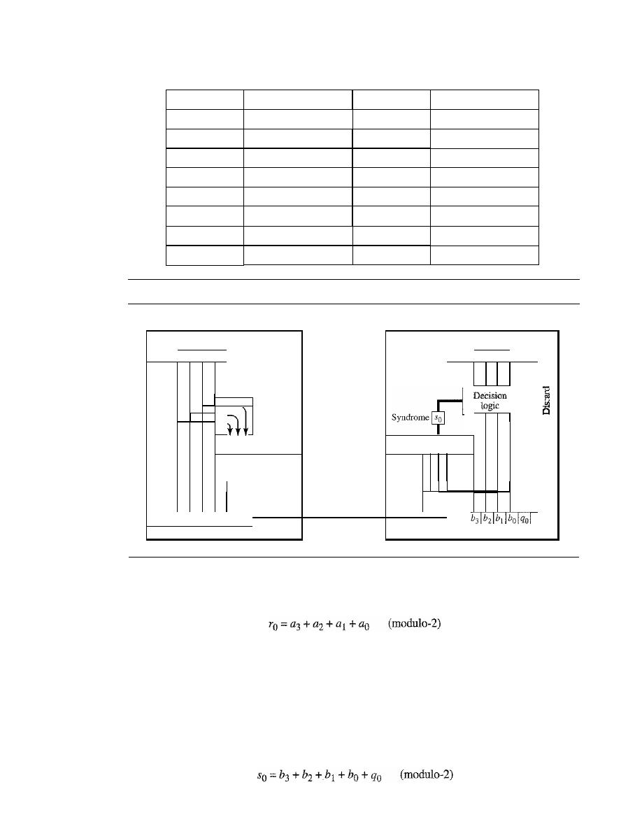
SECTION 10.3
LINEAR BLOCK CODES
279
Table 10.3
Simple parity-check code C(5, 4)
Datawords
Codewords
Datawords
Codewords
0000
00000
1000
10001
0001
00011
1001
10010
0010
00101
1010
10100
0011
00110
1011
10111
0100
01001
1100
11000
0101
01010
1101
11011
0110
01100
1110
11101
0111
01111
1111
11110
Figure 10.10
Encoder and decoder for simple parity-check code
Sender
Receiver
Encoder
Decoder
Dataword
Dataword
la31 a21 all aol
la31 a21 a
d
aol
Accept
I
Generator
I
I
Checker
I
J
t
l
Parity bit
Unreliable
la31 a21 all aol ro
transmission
Codeword
Codeword
This is normally done by adding the 4 bits of the dataword (modulo-2); the result is the
parity bit. In other words,
If
the number of 1s is even, the result is 0; if the number of 1s is odd, the result is 1.
In both cases, the total number of 1s in the codeword is even.
The sender sends the codeword which may
be
corrupted during transmission. The
receiver receives a 5-bit word. The checker at the receiver does the same thing as the gen-
erator in the sender with one exception: The addition is done over all 5 bits. The result,
which is called the
syndrome,
is just 1 bit. The syndrome is
0
when the number of Is
in
the
received codeword is even; otherwise, it is 1.

280
CHAPTER 10
ERROR DETECTION AND CORRECTION
The syndrome is passed to the decision logic analyzer. If the syndrome is 0, there is
no error in the received codeword; the data portion of the received codeword is accepted
as the dataword; if the syndrome is 1, the data portion of the received codeword is dis-
carded. The dataword is not created.
Example 10.12
Let us look at some transmission scenarios. Assume the sender sends the dataword 1011. The code-
word created from this dataword is 10111, which is sent to the receiver. We examine five cases:
1. No error occurs; the received codeword is 10111. The syndrome is O. The dataword 1011 is
created.
2. One single-bit error changes
aI'
The received codeword is 10011. The syndrome is 1. No
dataword is created.
3.
One single-bit error changes
roo
The received codeword is 10110. The syndrome is 1. No data-
word is created. Note that although none of the dataword bits are corrupted, no dataword is
created because the code is not sophisticated enough to show the position of the corrupted bit.
4. An error changes
ro
and a second error changes
a3'
The received codeword is 00110. The syn-
drome is
O.
The dataword 0011 is created at the receiver. Note that here the dataword is
wrongly created due to the syndrome value. The simple parity-check decoder cannot detect an
even number of errors. The errors cancel each other out and give the syndrome a value of
O.
5. Three bits-a3,
az, and aI-are changed by errors. The received codeword is 01011. The
syndrome is 1. The dataword is not created. This shows that the simple parity check, guaran-
teed to detect one single error, can also find any odd number of errors.
A simple parity-check code can detect an odd number of errors.
A better approach is the
two-dimensional parity check.
In this method, the data-
word is organized in a table (rows and columns).
In
Figure 10.11, the data to be sent, five
7-bit bytes, are put in separate rows. For each row and each column, 1 parity-check bit is
calculated. The whole table is then sent to the receiver, which finds the syndrome for each
row and each column. As Figure 10.11 shows, the two-dimensional parity check can
detect up to three errors that occur anywhere in the table (arrows point to the locations of
the created nonzero syndromes). However, errors affecting 4 bits may not be detected.
Hamming Codes
Now let us discuss a category of error-correcting codes called
Hamming codes.
These
codes were originally designed with
d
min
=
3, which means that they can detect up to two
errors or correct one single error. Although there are some Hamming codes that can cor-
rect more than one error, our discussion focuses on the single-bit error-correcting code.
First let us find the relationship between n and
k
in a Hamming code. We need to
choose an integer m
>=
3. The values of nand
k
are then calculated from mas n
=
2
m -
1
and
k :::
n - m.
The number of check bits r
=
m.
All Hamming codes discussed in this book have d
min
=
3.
The relationship between
m
and
n
in these codes is
n
=
2
m
1.
For example, if m
=
3, then n ::: 7 and
k:::
4. This is a Hamming code
C(7,
4) with d
min
=
3.
Table 10.4 shows the datawords and codewords for this code.
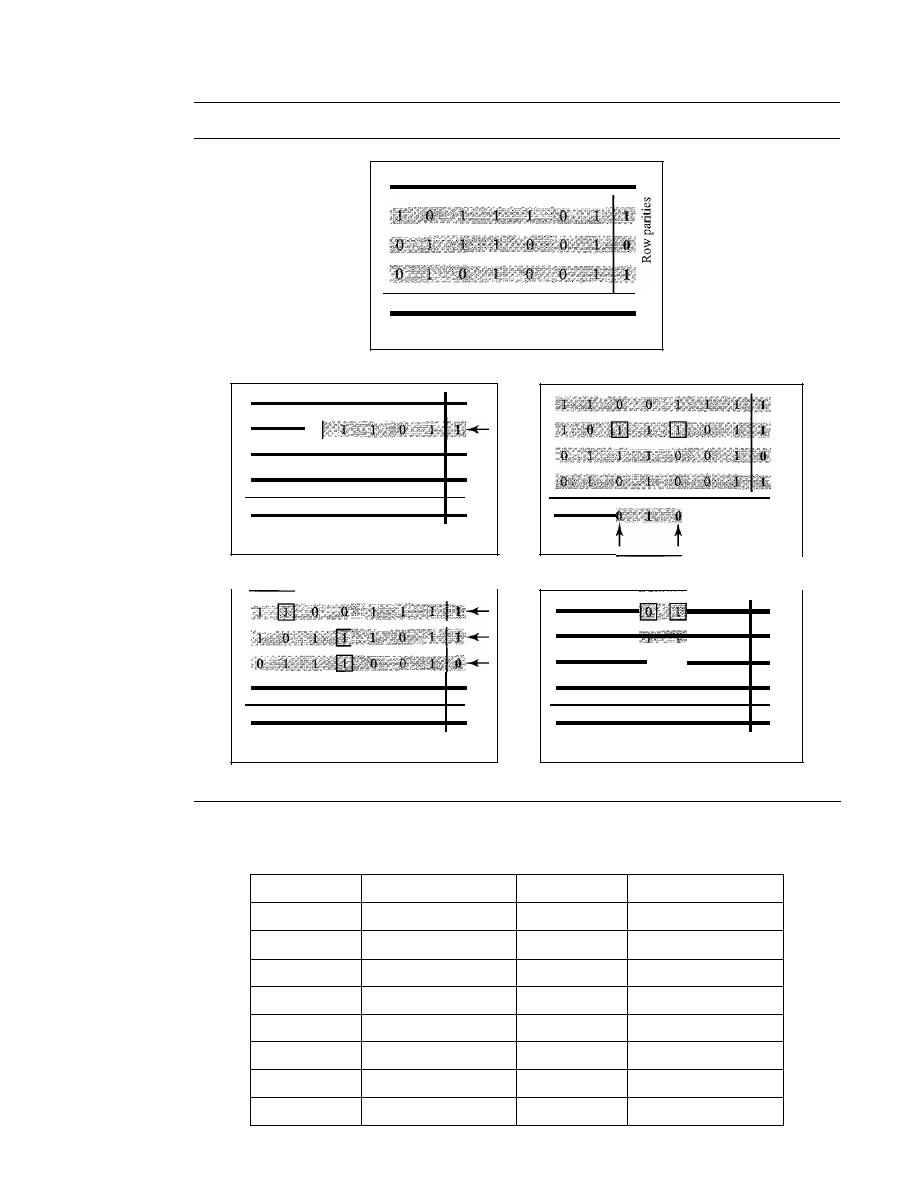
SECTION 10.3
LINEAR BLOCK CODES
281
Figure 10.11
Two-dimensional parity-check code
J
Column parities
a. Design of row and column parities
t
b. One error affects two parities
d. Three errors affect four parities
Table 10.4
Hamming code C(7, 4)
c. Two errors affect two parities
e. Four errors cannot be detected
Datawords
Codewords
Datawords
Codewords
0000
0000000
1000
1000110
0001
0001101
1001
1001011
0010
0010111
1010
1010001
0011
0011010
1011
10111 00
0100
0100011
1100
1100101
0101
01011 10
1101
1101000
0110
0110100
1110
1110010
0111
0111001
1111
1111111
282
CHAPTER 10
ERROR DETECTION AND CORRECTION
Figure 10.12 shows the structure of the encoder and decoder for this example.
Figure 10.12
The structure of the encoder and decoder for a Hamming code
Sender
Receiver
Encoder
Decoder
Dataword
Dataword
I
a31
azl a
1
I
ao
I
la31 azl atl
aol
Syndrome
I
Sz Stl
So
I
I
I
I
Checker
I
l
Unreliable
la3 lazlatl a
ol
r
2
I
TO
transmission
b
3
1
bzlbtl
b
o
qol
Codeword
Codeword
A copy of a 4-bit dataword is fed into the generator that creates three parity checks
ro, rl'
and
r2'
as shown below:
+ao
Tl
=
a3
+
az
+
al
T2=aI +aO+a3
modulo-2
modulo-2
modulo-2
In other words, each of the parity-check bits handles 3 out of the 4 bits of the data-
word. The total number of 1s in each 4-bit combination (3 dataword bits and 1 parity
bit) must be even. We are not saying that these three equations are unique; any three
equations that involve 3 of the 4 bits in the dataword and create independent equations
(a combination of two cannot create the third) are valid.
The checker in the decoder creates a 3-bit syndrome
(s2s1s0)
in which each bit is
the parity check for 4 out of the 7 bits in the received codeword:
So
b
z
+
b
i
+
b
o
+
qo
Sl
=
b
3
+
b
z
+
b
I
+
ql
8Z
b
l
+
b
o
+b
3
+qz
modulo-Z
modulo-2
modulo-2
The equations used by the checker are the same as those used by the generator with
the parity-check bits added to the right-hand side of the equation. The 3-bit syndrome
creates eight different bit patterns (000 to 111) that can represent eight different condi-
tions. These conditions define a lack of error or an error in 1 of the 7 bits of the received
codeword, as shown in Table 10.5.

SECTION 10.3
LINEAR BLOCK CODES
283
Table 10.5
Logical decision made by the correction logic analyzer a/the decoder
Syndrome
000
001
010
011
100
101
110
111
Error
None
ql
b
2
q2
b
o
b
3
b
l
Note that the generator is not concerned with the four cases shaded in Table 10.5
because there is either no error or an error in the parity bit. In the other four cases, 1 of
the bits must be flipped (changed from
0
to 1 or 1 to
0)
to find the correct dataword.
The syndrome values in Table
10.5
are based on the syndrome bit calculations. For
example, if
qo
is in error,
So
is the only bit affected; the syndrome, therefore, is 001. If
b
2
is in error,
So
and
s1
are the bits affected; the syndrome, therefore is OIl. Similarly, if
b
I
is in error, all 3 syndrome bits are affected and the syndrome is 111.
There are two points we need to emphasize here. First, if two errors occur during
transmission, the created dataword might not be the right one. Second, if we want to
use the above code for error detection, we need a different design.
Example 10.13
Let us trace the path of three datawords from the sender to the destination:
1.
The dataword
0100
becomes the codeword
0100011.
The codeword
01 00011
is received.
The syndrome is
000
(no error), the final dataword is
0100.
2. The dataword
0111
becomes the codeword
0111001.
The codeword
0011001
is received.
The syndrome is
011.
According to Table
10.5,
b
2
is in error. After flipping
b
2
(changing the
1
to
0),
the final dataword is
0111.
3.
The dataword
1101
becomes the codeword
1101000.
The codeword
0001000
is received
(two errors). The syndrome is
101,
which means that
b
o
is in error. After flipping
b
a,
we get
0000,
the wrong dataword. This shows that our code cannot correct two errors.
Example 10.14
We need a dataword of at least 7 bits. Calculate values of
k
and
n
that satisfy this requirement.
Solution
We need to make
k
=
n - m
greater than or equal to 7, or
2
1n
-
1 -
m
7.
1.
If
we set
m
=
3,
the result is
n
=
2
3
-
1 and
k
=
7 - 3, or 4, which is not acceptable.
2.
If
we set
m
=
4, then
n
=
2
4
-
1
=
15
and
k
=
15 -
4
=
11,
which satisfies the condition. So the
code is C(l5,
11).
There are methods to make the dataword a specific size, but the discussion
and implementation are beyond the scope of this book.
Performance
A Hamming code can only correct a single error or detect a double error. However,
there is a way to make it detect a burst error, as shown in Figure 10.13.
The key is to split a burst error between several codewords, one error for each
codeword. In data communications, we normally send a packet or a frame of data. To
make the Hamming code respond to a burst error of size
N,
we need to make
N
codewords out
of our frame. Then, instead of sending one codeword at a time, we arrange the codewords in a
table and send the bits
in
the table a column at a time.
In
Figure 10.13, the bits are sent colunm
by column (from the left).
In
each column, the bits are sent from the bottom to the top.
In
this
way, a frame is made out of the four codewords and sent to the receiver. Figure 10.13 shows
284
CHAPTER 10
ERROR DETECTION AND CORRECTION
Figure 10.13
Burst error correction using Hamming code
Sender
Codeword 4
Codeword
3
Receiver
Codeword 4
Codeword
3
Codeword
2
1
Codeword
1 1
Burst elTor
A
data unit in transit
COlTUpted bits
that when a burst error of size 4 corrupts the frame, only
1
bit from each codeword is cor-
rupted. The corrupted bit
in
each codeword can then easily be corrected at the receiver.
10.4
CYCLIC CODES
Cyclic codes are special linear block codes with one extra property. In a cyclic code, if
a codeword is cyclically shifted (rotated), the result is another codeword. For example,
if 1011000 is a codeword and we cyclically left-shift, then 0110001 is also a codeword.
In this case, if we call the bits in the first word
ao
to
a6'
and the bits in the second word
b
o
to
b
6,
we can shift the bits by using the following:
In the rightmost equation, the last bit of the first word is wrapped around and
becomes the first bit of the second word.
Cyclic Redundancy Check
We can create cyclic codes to correct errors. However, the theoretical background
required is beyond the scope of this book. In this section, we simply discuss a category
of cyclic codes called the cyclic redundancy check (CRC) that is used in networks
such as LANs and WANs.
SECTION 10.4
CYCUC CODES
285
Table 10.6 shows an example of a CRC code. We can see both the linear and cyclic
properties of this code.
Table 10.6
A CRC code with C(7,
4)
Dataword
Codeword
Dataword
0000
0000000
1000
1000101
0001
0001011
1001
1001110
0010
0010110
1010
1010011
0011
0011101
1011
1011000
0100
0100111
1100
1100010
0101
0101100
1101
1101001
0110
0110001
1110
1110100
0111
0111010
1111
1111111
Figure 10.14 shows one possible design for the encoder and decoder.
Figure 10.14
CRC encoder and decoder
Sender
Receiver
Dataword
Decoder
Unreliable
transmission
Dataword
000
Encoder
In
the encoder, the dataword has k bits (4 here); the codeword has
n
bits (7 here).
The size of the dataword is augmented by adding n -
k
(3 here) Os to the right-hand side
of the word. The n-bit result is fed into the generator. The generator uses a divisor of
size n - k
+
I (4 here), predefined and agreed upon. The generator divides the aug-
mented dataword by the divisor (modulo-2 division). The quotient ofthe division is dis-
carded; the remainder
(r2rl ro)
is appended to the dataword to create the codeword.
The decoder receives the possibly corrupted codeword. A copy of all n bits is fed to
the checker which is a replica of the generator. The remainder produced by the checker
286
CHAPTER 10
ERROR DETECTION AND CORRECTiON
is a syndrome of n -
k
(3 here) bits, which is fed to the decision logic analyzer. The ana-
lyzer has a simple function. If the syndrome bits are all as, the 4 leftmost bits of the
codeword are accepted as the dataword (interpreted as no error); otherwise, the 4 bits
are discarded (error).
Encoder
Let us take a closer look at the encoder. The encoder takes the dataword and augments
it with
n -
k number of as.
It
then divides the augmented dataword by the divisor, as
shown in Figure 10.15.
Figure 10.15
Division in CRC encoder
Division
Dalaword
11
0 0 1
I
Quotient
1 0 1 0
Divisor
1 0 1 1) I 0 0 1
1
0 1 1
Dividend:
augmenled
dataword
Leftmost bit 0:
use 0000 divisor
Leftmost bit 0:
use 0000 divisor
o
1 0 0
o
0 0 0
1
0 0 0
1 0 1 1
o
1 1 0
0 0 0 0
I
1 1 0
I
Remainder
Codeword
11
0 0
1
'-1-1
-0-1
Dataword Remainder
The process of modulo-2 binary division is the same as the familiar division pro-
cess we use for decimal numbers. However, as mentioned at the beginning of the
chapter, in this case addition and subtraction are the same. We use the XOR operation
to do both.
As in decimal division, the process is done step by step. In each step, a copy of the
divisor is XORed with the 4 bits of the dividend. The result of the XOR operation
(remainder) is 3 bits (in this case), which is used for the next step after 1 extra bit is
pulled down to make it 4 bits long. There is one important point we need to remember
in this type of division.
If
the leftmost bit of the dividend (or the part used in each step)
is 0, the step cannot use the regular divisor; we need to use an all-Os divisor.
When there are no bits left to pull down, we have a result. The 3-bit remainder
forms the check bits
(r2' rl'
and
ro).
They are appended to the dataword to create the
codeword.
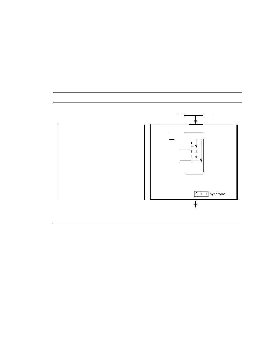
SECTION 10.4
CYCLIC CODES
287
Decoder
The codeword can change during transmission. The decoder does the same division
process as the encoder. The remainder of the division is the syndrome.
If
the syndrome
is all Os, there is no error; the dataword is separated from the received codeword and
accepted. Otherwise, everything is discarded. Figure 10.16 shows two cases: The left-
hand figure shows the value of syndrome when no error has occurred; the syndrome is
000. The right-hand part of the figure shows the case in which there is one single error.
The syndrome is not all Os (it is OIl).
Figure 10.16
Division in the CRC decoder for two cases
Codeword 11
o
0
011
1 0
I
Division
I 0
I 0
1 0 1 1) 1 0 0
o
1 1
o
_Codeword
1 0 1
0
I
I 1
0
0
o ()
1
I
0
1
o
0 0
0 1 1
D a t a w o r d _
discarded
Divisor
You may be wondering how the divisor] 011 is chosen. Later in the chapter we present
some criteria, but in general it involves abstract algebra.
Hardware Implementation
One of the advantages of a cyclic code is that the encoder and decoder can easily and
cheaply be implemented in hardware by using a handful of electronic devices. Also, a
hardware implementation increases the rate of check bit and syndrome bit calculation.
In this section, we try to show, step by step, the process. The section, however, is
optional and does not affect the understanding of the rest of the chapter.
Divisor
Let us first consider the divisor. We need to note the following points:
1. The divisor is repeatedly XORed with part of the dividend.
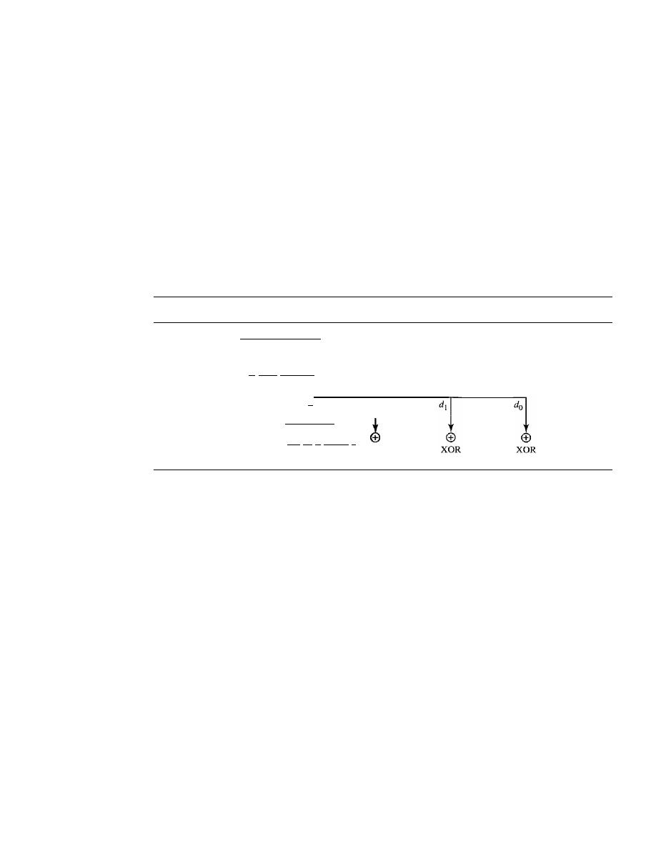
288
CHAPTER 10
ERROR DETECTION AND CORRECTION
2. The divisor has
n -
k
+
1 bits which either are predefined or are all Os. In other
words, the bits do not change from one dataword to another. In our previous exam-
ple, the divisor bits were either 1011 or 0000. The choice was based on the leftmost
bit of the part of the augmented data bits that are active in the XOR operation.
3. A close look shows that only
n -
k
bits of the divisor is needed in the XOR operation.
The leftmost bit is not needed because the result of the operation is always 0, no
matter what the value of this bit. The reason is that the inputs to this XOR operation
are either both Os or both 1s. In our previous example, only 3 bits, not 4, is actually
used in the XOR operation.
Using these points, we can make a fixed (hardwired) divisor that can be used for a cyclic
code if we know the divisor pattern. Figure 10.17 shows such a design for our previous
example. We have also shown the XOR devices used for the operation.
Figure 10.17
Hardwired design of the divisor in CRC
Leftmost bit of the part
of dividend involved
in XOR operation
•
Broken line:
this bit is always 0
XOR
Note that if the leftmost bit of the part of dividend to be used in this step is 1, the
divisor bits
(d
2
d
1
do)
are all; if the leftmost bit is 0, the divisor bits arc 000. The design
provides the right choice based on the leftmost bit.
Augmented Dataword
In our paper-and-pencil division process in Figure 10.15, we show the augmented data-
word as fixed in position with the divisor bits shifting to the right, 1 bit in each step.
The divisor bits are aligned with the appropriate part of the augmented dataword. Now
that our divisor is fixed, we need instead to shift the bits of the augmented dataword to the
left (opposite direction) to align the divisor bits with the appropriate part. There is no
need to store the augmented dataword bits.
Remainder
In our previous example, the remainder is 3 bits
(n -
k
bits in general) in length. We can
use three registers (single-bit storage devices) to hold these bits. To find the final
remainder of the division, we need to modify our division process. The following is the
step-by-step process that can be used to simulate the division process in hardware (or
even in software).
1. We assume that the remainder is originally all Os (000 in our example).
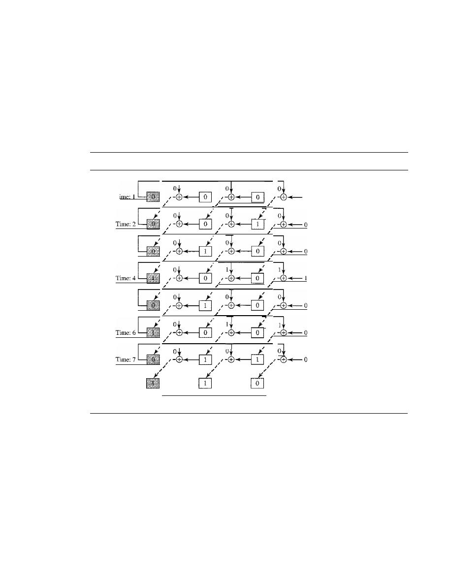
SECTION 10.4
CYCLIC CODES
289
2. At each time click (arrival of 1 bit from an augmented dataword), we repeat the
following two actions:
a. We use the leftmost bit to make a decision about the divisor (011 or 000).
b. The other 2 bits of the remainder and the next bit from the augmented dataword
(total of 3 bits) are XORed with the 3-bit divisor to create the next remainder.
Figure 10.18 shows this simulator, but note that this is not the final design; there will be
more improvements.
Figure 10.18
Simulation of division in CRC encoder
Augmented dataword
I
0
0
0
0
0
TIme:
I
,
0
0
0
00
Time: 3
,
1
0
0
0
,
0
0
0
0
Time: 5
0
0
.
0
0
1
I
Final remainder
At each clock tick, shown as different times, one of the bits from the augmented
dataword is used in the XOR process. If we look carefully at the design, we have seven
steps here, while in the paper-and-pencil method we had only four steps. The first three
steps have been added here to make each step equal and to make the design for each step
the same. Steps 1, 2, and 3 push the first 3 bits to the remainder registers; steps 4, 5, 6,
and 7 match the paper-and-pencil design. Note that the values in the remainder register
in steps 4 to 7 exactly match the values in the paper-and-pencil design. The final remain-
der is also the same.
The above design is for demonstration purposes only.
It
needs simplification to be
practical. First, we do not need to keep the intermediate values of the remainder bits;
we need only the final bits. We therefore need only 3 registers instead of 24. After the
XOR operations, we do not need the bit values of the previous remainder. Also, we do
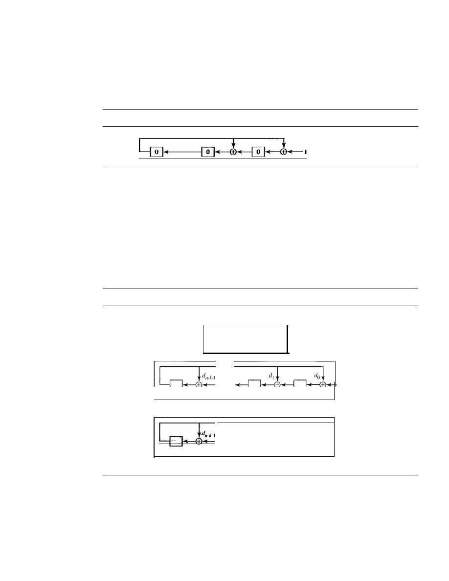
290
CHAPTER
10
ERROR DETECTION AND CORRECTION
not need 21 XOR devices; two are enough because the output of an XOR operation in
which one of the bits is 0 is simply the value of the other bit. This other bit can be used
as the output. With these two modifications, the design becomes tremendously simpler
and less expensive, as shown in Figure 10.19.
Figure 10.19
The CRC encoder design using shift registers
Augmented dataword
o
0
1
0 0 0
We need, however, to make the registers shift registers. A I-bit shift register holds
a bit for a duration of one clock time. At a time click, the shift register accepts the bit at
its input port, stores the new bit, and displays it on the output port. The content and the
output remain the same until the next input arrives. When we connect several I-bit shift
registers together, it looks as if the contents of the register are shifting.
General Design
A general design for the encoder and decoder is shown in Figure 10.20.
Figure 10.20
General design of encoder and decoder of a CRC code
Note:
The divisor line and XOR are
missing
if
the corresponding
bit in the divisor is
O.
Dataword
rn_k_l
r l
Yo
a. Encoder
Received
...
codeword
+
sn-k-l
sl
So
b. Decoder
Note that we have
n - k
I-bit shift registers in both the encoder and decoder. We
have up to n - k XOR devices, but the divisors normally have several Os in their pattern,
which reduces the number of devices. Also note that, instead of augmented datawords,
we show the dataword itself as the input because after the bits in the dataword are all
fed into the encoder, the extra bits, which all are Os, do not have any effect on the right-
most XOR. Of course, the process needs to be continued for another
n - k
steps before
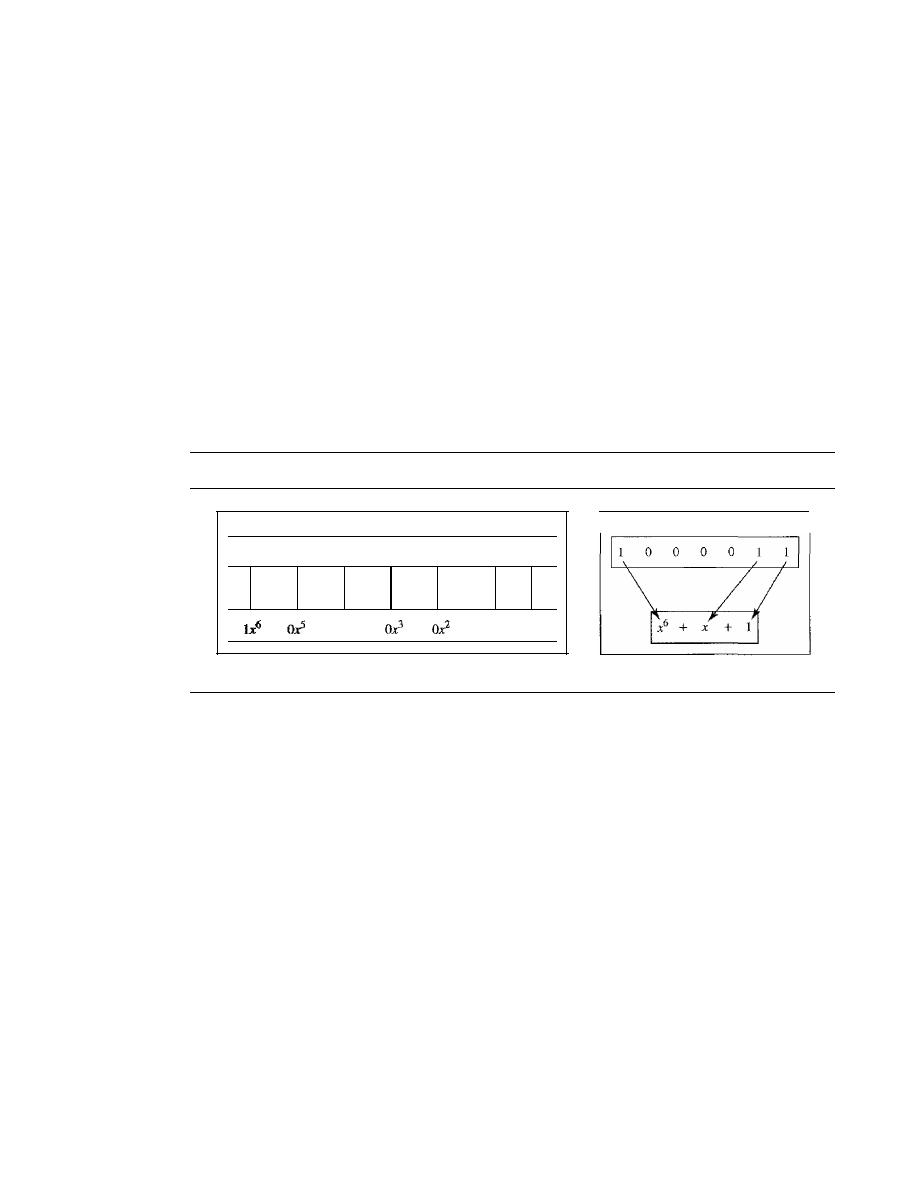
SECTION 10.4
CYCLIC CODES
291
the check bits are ready. This fact is one of the criticisms of this design. Better schemes
have been designed to eliminate this waiting time (the check bits are ready after k steps),
but we leave this as a research topic for the reader. In the decoder, however, the entire
codeword must be fed to the decoder before the syndrome is ready.
Polynomials
A better way to understand cyclic codes and how they can be analyzed is to represent
them as polynomials. Again, this section is optional.
A pattern of Os and 1s can be represented as a polynomial with coefficients of 0 and
1. The power of each term shows the position of the bit; the coefficient shows the value
of the bit. Figure 10.21 shows a binary pattern and its polynomial representation. In Fig-
ure 10.21a we show how to translate a binary pattern to a polynomial; in Figure 1O.21b
we show how the polynomial can be shortened by removing all terms with zero coeffi-
cients and replacing
xl
by
x
and
xO
by 1.
Figure 10.21
A polynomial to represent a binary word
I
1
I
0
I
0
I
0
I
0
I
1
I
1
I
I
+
+
ox
4
+
+
+
Ix
l
+
Ixo
I
a. Binary pattern and polynomial
b. Short form
Figure 10.21 shows one immediate benefit; a 7-bit pattern can be replaced by three
terms. The benefit is even more conspicuous when we have a polynomial such as x
23
+
X
3
+
1.
Here the bit pattern is 24 bits in length (three Is and twenty-one Os) while the
polynomial is just three terms.
Degree of a Polynomial
The degree of a polynomial is the highest power in the polynomial. For example, the
degree of the polynomial
x
6
+
x
+
1 is 6. Note that the degree of a polynomial is 1 less
that the number of bits in the pattern. The bit pattern in this case has 7 bits.
Adding and Subtracting Polynomials
Adding and subtracting polynomials in mathematics are done by adding or subtracting
the coefficients of terms with the same power. In our case, the coefficients are only 0
and 1, and adding is in modulo-2. This has two consequences. First, addition and sub-
traction are the same. Second, adding or subtracting is done by combining terms and
deleting pairs of identical terms. For example, adding x
5
+
x
4
+
x
2
and x
6
+
x
4
+
x
2
gives
just x
6
+
x
5
.
The terms x
4
and x
2
are deleted. However, note that if we add, for example,
three polynomials and we get x
2
three times, we delete a pair of them and keep the third.

292
CHAPTER 10
ERROR DETECTION AND CORRECTION
Multiplying or Dividing Terms
In this arithmetic, multiplying a term by another term is very simple; we just add the
powers. For example,
x
3
x
x
4
is
x
7
,
For dividing, we just subtract the power of the sec-
ond term from the power of the first. For example, x
5
1x
2
is x
3
.
Multiplying Two Polynomials
Multiplying a polynomial by another is done term by term. Each term of the first polyno-
mial must be multiplied by all terms of the second. The result, of course, is then simplified,
and pairs of equal terms are deleted. The following is an example:
+x+
1)
=x
7
+x
6
+x
3
+x
Dividing One Polynomial by Another
Division of polynomials is conceptually the same as the binary division we discussed
for an encoder. We divide the first term of the dividend by the first term of the divisor to
get the first term of the quotient. We multiply the term in the quotient by the divisor and
subtract the result from the dividend. We repeat the process until the dividend degree is
less than the divisor degree. We will show an example of division later in this chapter.
Shifting
A binary pattern is often shifted a number of bits to the right or left. Shifting to the left
means adding extra Os as rightmost bits; shifting to the right means deleting some right-
most bits. Shifting to the left is accomplished by multiplying each term of the polynomial
by
where m is the number of shifted bits; shifting to the right is accomplished by
dividing each term of the polynomial by
The following shows shifting to the left and
to the right. Note that we do not have negative powers in the polynomial representation.
Shifting left 3 bits:
Shifting right 3 bits:
10011 becomes 10011000
10011 becomes 10
x
4
+
x
+
1 becomes
x
7
+
x
4
+
x
4
+
x
+
1 becomes
x
When we augmented the dataword in the encoder of Figure 10.15, we actually
shifted the bits to the left. Also note that when we concatenate two bit patterns, we shift
the first polynomial to the left and then add the second polynomial.
Cyclic Code Encoder Using Polynomials
Now that we have discussed operations on polynomials, we show the creation of a code-
word from a dataword. Figure 10.22 is the polynomial version of Figure 10.15. We can
see that the process is shorter. The dataword 1001 is represented as x
3
+
1. The divisor
1011 is represented as
x
3
+
x
+
1. To find the augmented dataword, we have left-shifted
the dataword 3 bits (multiplying by
The result is
x
6
+
x
3
.
Division is straightforward.
We divide the first term of the dividend, x
6,
by the first term of the divisor, x
3.
The first
term of the quotient is then x
6
/x
3,
or x
3
.
Then we multiply x
3
by the divisor and subtract
(according to our previous definition of subtraction) the result from the dividend. The
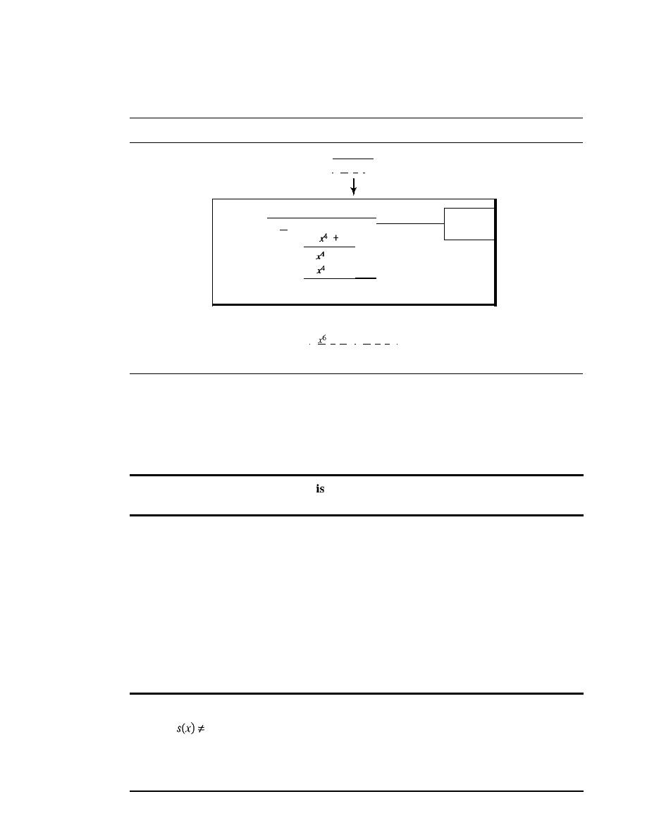
SECTION 10.4
CYCLiC CODES
293
result is
x
4
,
with a degree greater than the divisor's degree; we continue to divide until
the degree of the remainder is less than the degree of the divisor.
Figure 10.22
CRC division using polynomials
Dataword
I
x
3
+
1
Divisor
x
3
+
x
Dividend:
x
3
+
x
+
I )
x
6
+
x
3
augmented
x
6
+
x
3
dataword
+
x
2
+
x
I
x
2
+
x
I
Remainder
Codeword
I
+
x
3
I
xl
+
x
I
Dataword Remainder
It
can be seen that the polynomial representation can easily simplify the operation
of division in this case, because the two steps involving all-Os divisors are not needed
here. (Of course, one could argue that the all-Os divisor step can also be eliminated in
binary division.) In a polynomial representation, the divisor is normally referred to as
the generator polynomial
t(x).
The divisor in a cyclic code
normally called the generator polynomial
or simply the generator.
Cyclic Code Analysis
We can analyze a cyclic code to find its capabilities by using polynomials. We define
the following,
wheref(x)
is a polynomial with binary coefficients.
Dataword:
d(x)
Syndrome:
sex)
Codeword:
c(x)
Error:
e(x)
Generator:
g(x)
If
sex)
is not zero, then one or more bits is corrupted. However, if
sex)
is zero, either
no bit is corrupted or the decoder failed to detect any errors.
In a cyclic code,
I.
If
0, one or more bits is corrupted.
2.
If sex)
=
0, either
a. No bit is corrupted. or
b. Some bits are corrupted, but the decoder failed to detect them.

294
CHAPTER 10
ERROR DETECTION AND CORRECTION
In our analysis we want to find the criteria that must be imposed on the generator,
g(x)
to detect the type of error we especially want to be detected. Let us first find the
relationship among the sent codeword, error, received codeword, and the generator.
We can say
Received codeword
=
c(x)
+
e(x)
In other words, the received codeword is the sum of the sent codeword and the error.
The receiver divides the received codeword by
g(x)
to get the syndrome. We can write
this as
Received codeword
=
+
e(x)
g(x)
g(x)
g(x)
The first term at the right-hand side of the equality does not have a remainder
(according to the definition of codeword). So the syndrome is actually the remainder of
the second term on the right-hand side.
If
this term does not have a remainder (syn-
drome
=
0), either
e(x)
is 0 or
e(x)
is divisible by
g(x).
We do not have to worry about
the first case (there is no error); the second case is very important. Those errors that are
divisible by
g(x)
are not caught.
In a cyclic code, those
e(x)
errors that are divisible by
g(x)
are not caught.
Let us show some specific errors and see how they can be caught by a well-
designed
g(x).
Single-Bit Error
What should be the structure of
g(x)
to guarantee the detection of a single-bit error? A
single-bit error is
e(x)
=
xi,
where i is the position of the bit. If a single-bit error is caught,
then
xi
is not divisible by
g(x).
(Note that when we say
not
divisible, we mean that there
is a remainder.) If
g(x)
at least two terms (which is normally the case) and the coeffi-
cient of
xO
is not zero (the rightmost bit is 1), then
e(x)
cannot be divided by
g(x).
the generator has more than one term and the coefficient of
xO
is 1,
all single errors can be caught.
Example 10.15
Which of the following
g(x)
values guarantees that a single-bit error is caught? For each case,
what is the error that cannot be caught?
a.
x
+
1
b.
x
3
c.
1
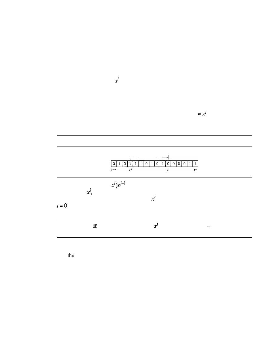
SECTION 10.4
CYCLIC CODES
295
Solution
a. No
xi
can be divisible by
x
+
1. In other words,
xi/ex
+
1) always has a remainder. So the
syndrome is nonzero. Any single-bit error can be caught.
b. If
i
is equal to or greater than 3,
xi
is divisible by
g(x).
The remainder of
x i/x
3
is zero, and
the receiver is fooled into believing that there is no error, although there might be one.
Note that in this case, the corrupted bit must be in position 4 or above. All single-bit
errors in positions I to 3 are caught.
c. All values of
i
make
divisible by
g(x).
No single-bit error can be caught.
In
addition, this
g(x)
is useless because it means the codeword is just the dataword augmented withn -
k
zeros.
Two Isolated Single-Bit Errors
Now imagine there are two single-bit isolated errors. Under what conditions can this
type of error be caught? We can show this type of error as
e(x)
+
xi.
The values of
i
and
j
define the positions of the errors, and the difference
j - i
defines the distance
between the two errors, as shown in Figure 10.23.
Figure 10.23
Representation o/two isolated single-bit errors using polynomials
I'
Difference:
j -
i
We can write
e(x)
=
+
1). If
g(x)
has more than one term and one term is
xo,
it
cannot divide
as we saw in the previous section. So if
g(x)
is to divide
e(x),
it must divide
x
j
-
i
+
1. In other words,
g(x)
must not divide
+
1, where
t
is between 0 and
n -
1. However,
is meaningless and
t
=
I is needed as we will see later. This means
t
should be between
2andn-1.
a generator cannot divide
+
1
(t
between 0 and
n
1),
then all isolated double errors can be detected.
Example 10.16
Find
status of the following generators related to two isolated, single-bit errors.
a.
x+ 1
b. x
4
+
I
c. x
7
+
x
6
+
1
d.
x
ls
+x
I4
+1
Solution
a. This is a very poor choice for a generator. Any two errors next to each other cannot be detected.
b. This generator cannot detect two errors that are four positions apart. The two errors can
be anywhere, but if their distance is 4, they remain undetected.
c. This is a good choice for this purpose.
d. This polynomial cannot divide any error of
typex
t
+
1 if
t is less than 32,768. This means
that a codeword with two isolated errors that are next to each other or up to 32,768 bits
apart can be detected by this generator.

296
CHAPTER 10
ERROR DETECTION AND CORRECTION
Odd Numbers of Errors
A generator with a factor of
x
+
1 can catch all odd numbers of errors. This means that
we need to make
x
+
1 a factor of any generator. Note that we are not saying that the
generator itself should be
x
+
1; we are saying that it should have a factor of
x
+
1.
If
it
is only
x
+
1, it cannot catch the two adjacent isolated errors (see the previous section).
For example, x
4
+
x
2
+
X
+
1 can catch all odd-numbered errors since it can be written
as a product of the two polynomials x
+
1 and x
3
+
x
2
+
1.
A generator that contains a factor of
x
+
1 can detect all odd-numbered errors.
Burst Errors
Now let us extend our analysis to the burst error, which is the most important of all. A
burst error is of the form
e(x)
=
+ ... +
xi).
Note the difference between a burst error
and two isolated single-bit errors. The first can have two terms or more; the second can
only have two terms. We can factor out
xi
and write the error as
+ ... +
1). If our
generator can detect a single error (minimum condition for a generator), then it cannot
divide
xi.
What we should worry about are those generators that divide
+ ... +
1. In
other words, the remainder of
+ ... +
1)/(x
r
+ ...
+
1) must not be zero. Note that
the denominator is the generator polynomial. We can have three cases:
1.
If j -
i
<
r, the remainder can never be zero. We can write
j -
i
=
L -
1, where
L
is
the length of the error. So
L -
1
<
r
or
L
<
r
+
1 or
L
r.
This means all burst errors
with length smaller than or equal to the number of check bits
r
will be detected.
2. In some rare cases, if
j
i
=
r,
or
L
=
r
+
1, the syndrome is 0 and the error is unde-
tected.
It
can be proved that in these cases, the probability of undetected burst error of
length
r
+
1 is
For example, if our generator is
x
l4
+
+
1, in which
r
=
14, a
burst error of length
L
=
15 can slip by undetected with the probability of
(1/2)14-1
or
almost 1 in 10,000.
3. In some rare cases, if
j -
i
>
r,
or
L
>
r
+
1, the syndrome is 0 and the error is unde-
tected.
It
can be proved that in these cases, the probability of undetected burst error
of length greater than
r
+
1
is
For example, if our generator is
x
14
+
x
3
+
1, in
which
r
=
14, a burst error of length greater than 15 can slip by undetected with the
probability of
(112)14
or almost 1 in 16,000 cases.
o
All burst errors with
L
r will be detected.
o
All burst errors with
L
=
r
+
1 will be detected with probability 1 -
(112/-
1•
o
All burst errors with
L
>
r
+
1 will be detected with probability 1- (1/2[.
Example 10.17
Find the suitability of the following generators in relation to burst errors of different lengths.
a.
x
6
+
1
b.
x
I8
+
x
7
+
x
+
1
c.
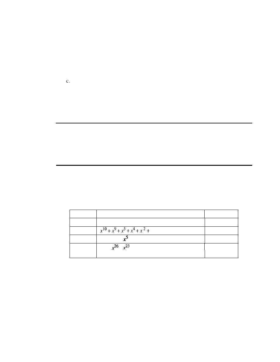
SECTION 10.4
CYCLIC CODES
297
Solution
a. This generator can detect all burst errors with a length less than or equal to 6 bits; 3 out
of 100 burst errors with length 7 will slip by; 16 out of 1000 burst errors of length 8 or
more will slip by.
b. This generator can detect all burst errors with a length less than or equal to 18 bits; 8 out
of 1 million burst errors with length 19 will slip by; 4 out of I million burst errors of
length 20 or more will slip by.
This generator can detect all burst errors with a length less than or equal to 32 bits; 5 out
of 10 billion burst errors with length 33 will slip by; 3 out of 10 billion burst errors of
length 34 or more will slip by.
Summary
We can summarize the criteria for a good polynomial generator:
A good polynomial generator needs to have the following characteristics:
1.
It
should have at least two terms.
2. The coefficient of the term
xO
should be 1.
3.
It
should not divide
Xl
+
1, for
t
between 2 and n - 1.
4.
It
should have the factor x
+
1.
Standard Polynomials
Some standard polynomials used by popular protocols for
eRe
generation are shown
in Table 10.7.
Table 10.7
Standard polynomials
Name
Polynomial
Application
CRC-8
x
S
+x
2
+x
+
1
ATM header
CRC-lO
I
ATMAAL
CRC-16
x
16
+
x
12
+
+
1
HDLC
CRC-32
x 32
+
+
+
x
22
+
x
16
+
x
12
+
xlI
+
x
lO
+
LANs
x
8
+
x
7
+
x
5
+
x
4
+
x
2
+
x
+
1
Advantages of Cyclic Codes
We have seen that cyclic codes have a very good performance in detecting single-bit
errors, double errors, an odd number of errors, and burst errors. They can easily be
implemented in hardware and software. They are especially fast when implemented in
hardware. This has made cyclic codes a good candidate for many networks.
Other Cyclic Codes
The cyclic codes we have discussed in this section are very simple. The check bits and
syndromes can be calculated by simple algebra. There are, however, more powerful
polynomials that are based on abstract algebra involving Galois fields. These are beyond

298
CHAPTER
10
ERROR DETECTION AND CORRECTION
the scope of this book. One of the most interesting of these codes is the
Reed-Solomon
code
used today for both detection and correction.
10.5
CHECKSUM
The last error detection method we discuss here is called the
checksum.
The checksum
is used in the Internet by several protocols although not at the data link layer. However,
we briefly discuss it here to complete our discussion on error checking.
Like linear and cyclic codes, the checksum is based on the concept of redundancy.
Several protocols still use the checksum for error detection as we will see in future
chapters, although the tendency is to replace it with a CRe. This means that the CRC is
also used in layers other than the data link layer.
Idea
The concept of the checksum is not difficult. Let us illustrate it with a few examples.
Example 10.18
Suppose our data is a list of five 4-bit numbers that we want to send to a destination. In addition
to sending these numbers, we send the sum of the numbers. For example, if the set of numbers is
(7,
11, 12, 0, 6), we send
(7,
11, 12,0,6,36), where 36 is the sum of the original numbers. The
receiver adds the five numbers and compares the result with the sum. If the two are the same,
the receiver assumes no error, accepts the five numbers, and discards the sum. Otherwise, there is
an error somewhere and the data are not accepted.
Example 10.19
We can make the job of the receiver easier if we send the negative (complement) of the sum,
called the
checksum.
In this case, we send
(7,
11, 12,0,6, -36). The receiver can add all the num-
bers received (including the checksum).
If
the result is 0, it assumes no error; otherwise, there is
an error.
One's Complement
The previous example has one major drawback. All of our data can be written as a 4-bit
word (they are less than 15) except for the checksum. One solution is to use
one's com-
plement
arithmetic. In this arithmetic, we can represent unsigned numbers between 0
and 2
n
-
1 using only n bits.
t
If
the number has more than n bits, the extra leftmost bits
need to be added to the
n
rightmost bits (wrapping). In one's complement arithmetic, a
negative number can be represented by inverting all bits (changing a 0 to a 1 and a 1 to
a 0). This is the same as subtracting the number from
2
n
-
1.
Example 10.20
How can we represent the number 21 in one's complement arithmetic using only four bits?
t
Although one's complement can represent both positive and negative numbers, we are concerned only with
unsigned representation here.
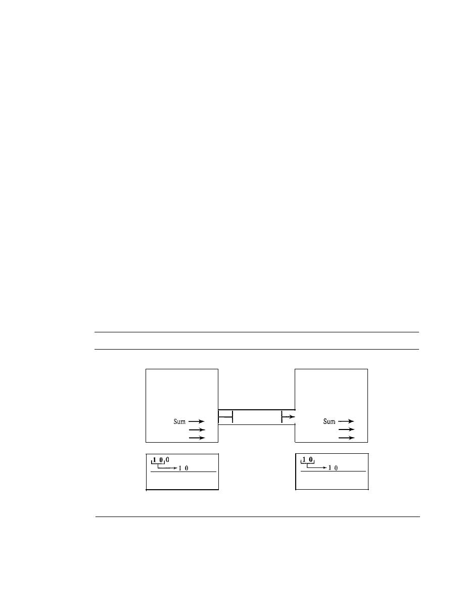
SECTION 10.5
CHECKSUM
299
Solution
The number 21 in binary is 1010 1 (it needs five bits). We can wrap the leftmost bit and add it to
the four rightmost bits. We have (0101
+
1)
=
0110 or 6.
Example 10.21
How can we represent the number -6 in one's complement arithmetic using only four bits?
Solution
In one's complement arithmetic, the negative or complement of a number is found by inverting
all bits. Positive 6 is 0110; negative 6 is 100 I. If we consider only unsigned numbers, this is 9. In
other words, the complement of 6 is 9. Another way to find the complement of a number in one's
complement arithmetic is to subtract the numberfrom 2
n
-
I (16 - 1 in this case).
Example 10.22
Let us redo Exercise 10.19 using one's complement arithmetic. Figure 10.24 shows the process at
the sender and at the receiver. The sender initializes the checksum to 0 and adds all data items and
the checksum (the checksum is considered as one data item and is shown in color). The result is
36. However, 36 cannot be expressed in 4 bits. The extra two bits are wrapped and added with
the sum to create the wrapped sum value 6. In the figure, we have shown the details in binary. The
sum is then complemented, resulting in the checksum value 9 (15 - 6
=
9). The sender now sends
six data items to the receiver including the checksum 9. The receiver follows the same procedure
as the sender. It adds all data items (including the checksum); the result is 45. The sum is
wrapped and becomes 15. The wrapped sum is complemented and becomes O. Since the value of
the checksum is 0, this means that the data is not corrupted. The receiver drops the checksum and
keeps the other data items.
If
the checksum is not zero, the entire packet is dropped.
Figure 10.24
Sender site
Receiver site
7
7
11
11
12
12
0
0
6
6
0
7, II, 12,0,6,9
9
36
45
Wrapped sum
6
Packet
Wrapped sum
15
Checksum
9
Checksum
0
1 0 0
o
1 1 0
100 1
36
6
9
1 1 0 1
1 1 1 1
o
0 0 0
45
15
o
Details of wrapping
and complementing
Details of wrapping
and complementing
Internet Checksum
Traditionally, the Internet has been using a 16-bit checksum. The sender calculates the
checksum by following these steps.
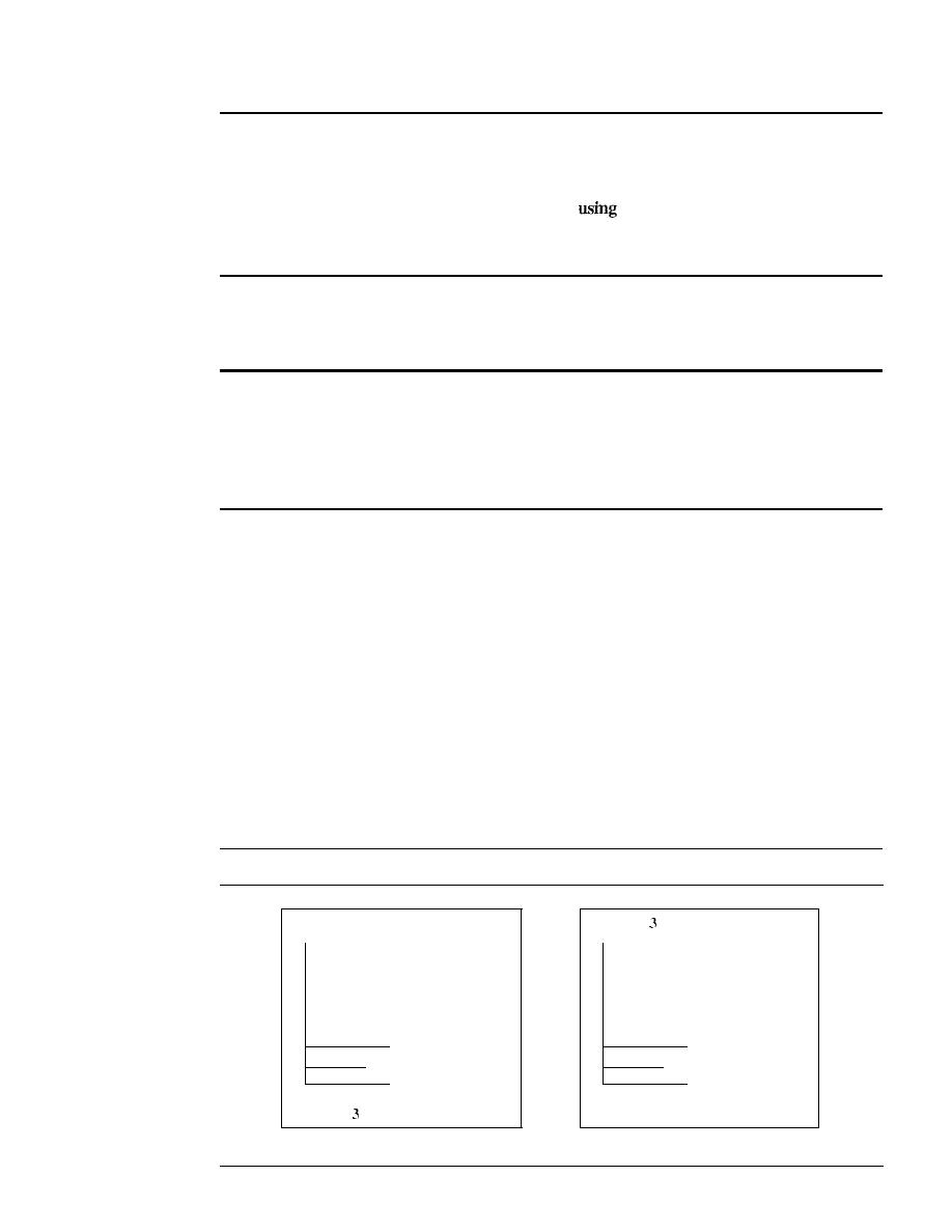
300
CHAPTER 10
ERROR DETECTION AND CORRECTION
Sender site:
1.
The message is divided into 16-bit words.
2. The value of the checksum word is set to O.
3. All words including the checksum are added
one's complement addition.
4. The sum is complemented and becomes the checksum.
5. The checksum is sent with the data.
The receiver uses the following steps for error detection.
Receiver site:
1. The message (including checksum) is divided into 16-bit words.
2. All words are added using one's complement addition.
3. The sum is complemented and becomes the new checksum.
4.
If
the value of checksum is 0, the message
is
accepted; otherwise, it is rejected.
The nature of the checksum (treating words as numbers and adding and comple-
menting them) is well-suited for software implementation. Short programs can be written
to calculate the checksum at the receiver site or to check the validity of the message at
the receiver site.
Example 10.23
Let us calculate the checksum for a text of 8 characters ("Forouzan"). The text needs to be divided
into 2-byte (l6-bit) words. We use ASCII (see Appendix A) to change each byte to a 2-digit hexa-
decimal number. For example, F is represented as Ox46 and
0
is represented as Ox6F. Figure 10.25
shows how the checksum is calculated at the sender and receiver sites. In part a of the figure,
the value of partial sum for the first column is Ox36. We keep the rightmost digit (6) and insert the
Figure 10.25
I
0
1
3
Carries
4
6
6
F
(Fo)
7
2
6
F
(ro)
7
5
7
A
luz)
6
1
6
E
(an)
0
0
0
0
Checksum (initial)
8
F
C
6
Sum (partial)
1
8
F C
7
Sum
7
0
8
Checksum (to send)
a. Checksum at the sender site
1
()
1
Carries
4
6
6
F
IFo)
7
2
6
F
(ro)
7
5
7
A
(uz)
6
1
6
E
(an)
7
0
3
8
Checksum (received)
F
F
F
E
Sum (partial)
1
F
F
F F
Sum
0
0
0
()
Checksum (new}
b. Checksum at the receiver site

SECTION fO.7
KEY TERMS
301
leftmost dight
(3)
as the carry in the second column. The process is repeated for each column.
Hexadecimal numbers are reviewed in Appendix B.
Note that if there is any corruption, the checksum recalculated by the receiver is not all as.
We leave this an exercise.
Performance
The traditional checksum uses a small number of bits (16)
to
detect errors in a message
of any size (sometimes thousands of bits). However, it is not as strong as the CRC in
error-checking capability. For example, if the value of one word is incremented and the
value of another word is decremented by the same amount, the two errors cannot be
detected because the sum and checksum remain the same. Also if the values of several
words are incremented but the total change is a multiple of 65535, the sum and the
checksum does not change, which means the errors are not detected. Fletcher and Adler
have proposed some weighted checksums, in which each word is multiplied by a
ber (its weight) that is related
to
its position in the text. This will eliminate the first
problem we mentioned. However, the tendency in the Internet, particularly in designing
new protocols, is
to
replace the checksum with a CRC.
10.6
RECOMMENDED READING
For more details about subjects discussed in this chapter, we recommend the following
books. The items in brackets [...] refer
to
the reference list at the end of the text.
Books
Several excellent book are devoted
to
error coding. Among them we recommend [Ham80],
[Zar02], [Ror96], and [SWE04].
RFCs
A discussion of the use of the checksum in the Internet can be found in RFC 1141.
10.7
KEY TERMS
block code
burst error
check bit
checksum
codeword
convolution code
cyclic code
cyclic redundancy check (CRC)
dataword
error
error correction
error detection
forward error correction
generator polynomial
Hamming code
Hamming distance
interference
linear block code
minimum Hamming distance
modular arithmetic

302
CHAPTER
10
ERROR DETECTION AND CORRECTION
modulus
one's complement
parity bit
parity-check code
polynomial
redundancy
Reed-Solomon
register
retransmission
shift register
single-bit error
syndrome
two-dimensional parity
check
10.8
SUMMARY
o
Data can be corrupted during transmission. Some applications require that errors be
detected and corrected.
o
In a single-bit error, only one bit in the data unit has changed. A burst error means
that two or more bits in the data unit have changed.
o
To detect or correct errors, we need to send extra (redundant) bits with data.
o
There are two main methods of error correction: forward error correction and correc-
tion by retransmission.
o
We can divide coding schemes into two broad categories: block coding and convo-
lution coding.
o
In coding, we need
to
use modulo-2 arithmetic. Operations in this arithmetic are very
simple; addition and subtraction give the same results. we use the XOR (exclusive
OR) operation for both addition and subtraction.
o
In block coding, we divide our message into blocks, each of k bits, called datawords.
We add
r
redundant bits
to
each block to make the length
n :::
k
+
r.
The resulting n-bit
blocks are called codewords.
o
In block coding, errors be detected by using the following two conditions:
a. The receiver has (or can find) a list of valid codewords.
b.
The original codeword has changed to an invalid one.
o
The Hamming distance between two words is the number of differences between
corresponding bits. The minimum Hamming distance is the smallest Hamming
distance between all possible pairs in a set of words.
o
To guarantee the detection of up to s errors in all cases, the minimum Hamming dis-
tance in a block code must be d
min :::
s
+
1. To guarantee correction of up to
t
errors in
all cases, the minimum Hamming distance in a block code must be d
min :::
2t
+
1.
o
In a linear block code, the exclusive OR (XOR) of any two valid codewords creates
another valid codeword.
o
A simple parity-check code is a single-bit error-detecting code in which n :::
k
+ 1
with d
min :::
2. A simple parity-check code can detect an odd number of errors.
o
All Hamming codes discussed in this book have d
min :::
3. The relationship between
m
and
n
in these codes is
n::: 2m -
1.
o
Cyclic codes are special linear block codes with one extra property. In a cyclic code,
if a codeword is cyclically shifted (rotated), the result is another codeword.

SECTION 10.9
PRACTICE SET
303
o
A category of cyclic codes called the cyclic redundancy check (CRC) is used in
networks such as LANs and WANs.
o
A pattern of Os and Is can be represented as a polynomial with coefficients of 0 and 1.
o
Traditionally, the Internet has been using a I6-bit checksum, which uses one's com-
plement
arithmetic. In this arithmetic, we can represent unsigned numbers between
o
and
2
n
-1
using only n bits.
10.9
PRACTICE SET
Review Questions
1. How does a single-bit error differ from a burst error?
2. Discuss the concept of redundancy in error detection and correction.
3. Distinguish between forward error correction versus error correction by retransmission.
4. What is the definition of a linear block code? What is the definition of a cyclic code?
5. What is the Hamming distance? What is the minimum Hamming distance?
6. How is the simple parity check related to the two-dimensional parity check?
7. In CRC, show the relationship between the following entities (size means the number
of bits):
The size of the dataword and the size of the codeword
b. The size of the divisor and the remainder
c. The degree of the polynomial generator and the size of the divisor
d. The degree of the polynomial generator and the size of the remainder
8. What kind of arithmetic is used to add data items in checksum calculation?
9. What kind of error is undetectable by the checksum?
10. Can the value of a checksum be all Os (in binary)? Defend your answer. Can the
value be allIs (in binary)? Defend your answer.
Exercises
11. What is the maximum effect of a 2-ms burst of noise on data transmitted at the fol-
lowing rates?
a. 1500 bps
b. 12 kbps
c. 100 kbps
d. 100 Mbps
12. Apply the exclusive-or operation on the following pair of patterns (the symbol
means XOR):
a. (10001)
(10000)
b. (10001)
(10001) (What do you infer from the result?)
c. (11100)
(00000) (What do you infer from the result?)
d. (10011)
(11111) (What do you infer from the result?)

304
CHAPTER 10
ERROR DETECTION AND CORRECTION
13. In Table 10.1, the sender sends dataword 10. A 3-bit burst error corrupts the
word. Can the receiver detect the error? Defend your answer.
14. In Table 10.2, the sender sends dataword 10.
If
a 3-bit burst
the first
three bits of the codeword, can the receiver detect the error? Defend your answer.
15. What is the Hamming distance for each of the following codewords:
a.
d
(10000, 00000)
b. d
(10101, 10000)
c.
d
(11111,11111)
d. d (000, 000)
16. Find the minimum Hamming distance for the following cases:
a. Detection of two
b. Correction of two errors.
c. Detection of 3 errors or correction of 2 errors.
d. Detection of 6 errors or correction of 2 errors.
17. Using the code in Table 10.2, what is the dataword if one of the following code-
words is received?
a. 01011
b.
11111
c. 00000
d.
11011
18. Prove that the code represented by Table 10.8 is not a linear code. You need to find
only one case that violates the linearity.
Table 10.8
Table for Exercise 18
Dataword
Codeword
00
00000
01
01011
10
10111
11
11111
19. Although it can mathematically be proved that a simple parity check code is a linear
code, use manual testing of linearity for five pairs of the codewords in Table 10.3 to
partially prove this fact.
20. Show that the Hamming code C(7,4) of Table lOA can detect two-bit
but not
necessarily three-bit error by testing the code in the following cases. The character
in the burst
means no
the character "E" means an error.
a. Dataword: 0100
Burst error:
b. Dataword: 0111
Burst error:
c. Dataword: 1111
Burst error:
d. Dataword: 0000
Burst

SECTION 10.9
PRACTICE SET
305
21. Show that the Hamming code C(7,4) of Table lOA can correct one-bit errors but
not more by testing the code in the following cases. The character
in the burst
error means no error; the character "E" means an error.
a. Dataword: 0100
Burst error:
b. Dataword: 0111
Burst error:
c. Dataword: 1111
Burst error:
d. Dataword: 0000
Burst error:
22. Although it can be proved that code in Table 10.6 is both linear and cyclic, use
only two tests to partially prove the fact:
a. Test the cyclic property on codeword 0101100.
b. Test the linear property on codewords 0010110 and 1111111.
23. We need a dataword of at least 11 bits. Find the values of
k
and
n in the Hamming
code
C(n, k)
with
d
min
3.
24. Apply the following operations on the corresponding polynomials:
a.
(x3
+
xl
+
X
+
1)
+
(x4
+
xl
+
x
+
1)
b.
(x
3
+
xl
+
x
+
1) -
(x
4
+
xl
+
x
+
1)
c.
(x
3
+
xl)
X
(x
4
+
x
2
+
x
+
1)
d.
(x
3
+
x
2
+
x
+
1) /
(x
2
+
1)
25. Answer the following questions:
a. What is the polynomial representation of 10111O?
b. What is the result of shifting 101110 three bits to the left?
c. Repeat part b using polynomials.
d. What is the result of shifting 101110 four bits to the right?
e. Repeat part d using polynomials.
26. Which of the following CRC generators guarantee the detection of a single bit
error?
a.
x
3
+
x
+
1
b.
x
4
+
xl
c.
1
d.
x
2
+
1
27. Referring to the CRC-8 polynomial in Table 10.7, answerthe following questions:
a. Does it detect a single error? Defend your answer.
b. Does it detect a burst error of size 6? Defend your answer.
c. What is the probability of detecting a burst error of size 9?
d. What is the probability of detecting a burst error of size 15?
28. Referring to the CRC-32 polynomial in Table 10.7, answer the following questions:
a. Does it detect a single error? Defend your answer.
b. Does it detect a burst error of size 16? Defend your answer.
c. What is the probability of detecting a burst error of size 33?
d. What is the probability of detecting a burst error of size 55?

306
CHAPTER 10
ERROR DETECTION AND CORRECTION
29. Assuming even parity, find the parity bit for each of the following data units.
a. 1001011
b.
0001100
1000000
d. 1110111
30. Given the dataword 1010011110 and the divisor 10111,
a. Show the generation of the codeword at the sender site (using binary division).
h. Show the checking of the codeword at the receiver site (assume no error).
3 I. Repeat Exercise 30 using polynomials.
A sender needs to send the four data items Ox3456, OxABCC, Ox02BC, and OxEEEE.
Answer the following:
a. Find the checksum at the sender site.
b. Find the checksum at the receiver site if there is no error.
Find the checksum at the receiver site if the second data item is changed to
OxABCE.
d. Find the checksum at the receiver site if the second data item is changed to
OxABCE and the third data item is changed to Ox02BA.
This problem shows a special case in checksum handling. A sender has two data
items to send: Ox4567 and OxBA98. What is the value of the checksum?

CHAPTER 11
Data Link Control
The two main functions of the data link layer are data link control and media access
control. The first, data link control, deals with the design and procedures for communi-
cation between two adjacent nodes: node-to-node communication. We discuss this
functionality in this chapter. The second function of the data link layer is media access
control, or how to share the link. We discuss this functionality in Chapter 12.
Data link control functions include framing, flow and error control, and software-
implemented protocols that provide smooth and reliable transmission of frames
between nodes. In this chapter, we first discuss framing, or how to organize the bits that
are carried by the physical layer. We then discuss flow and error control. A subset of
this topic, techniques for error detection and correction, was discussed in Chapter 10.
To implement data link control, we need protocols. Each protocol is a set of rules
that need to be implemented in software and run by the two nodes involved in data
exchange at the data link layer. We discuss five protocols: two for noiseless (ideal)
channels and three for noisy (real) channels. Those in the first category are not actually
implemented, but provide a foundation for understanding the protocols in the second
category.
After discussing the five protocol designs, we show how a bit-oriented protocol is
actually implemented by using the High-level Data Link Control (HDLC) Protocol as an
example. We also discuss a popular byte-oriented protocol, Point-to-Point Protocol (PPP).
11.1
FRAMING
Data transmission in the physical layer means moving bits in the form of a signal from
the source to the destination. The physical layer provides bit synchronization to ensure
that the sender and receiver use the same bit durations and timing.
The data link layer, on the other hand, needs to pack bits into frames, so that each
frame is distinguishable from another. Our postal system practices a type of framing.
The simple act of inserting a letter into an envelope separates one piece of information
from another; the envelope serves as the delimiter. In addition, each envelope defines
the sender and receiver addresses since the postal system is a many-to-many carrier
facility.
307

308
CHAPTER
11
DATA LINK CONTROL
Framing in the data link layer separates a message from one source to a destina-
tion, or from other messages to other destinations, by adding a sender address and a
destination address. The destination address defines where the packet is to go; the sender
address helps the recipient acknowledge the receipt.
Although the whole message could be packed in one frame, that is not normally
done. One reason is that a frame can be very large, making flow and error control very
inefficient. When a message is carried in one very large frame, even a single-bit error
would require the retransmission of the whole message. When a message is divided
into smaller frames, a single-bit error affects only that small frame.
Fixed-Size Framing
Frames can be of fixed or variable size. In fixed-size framing, there is no need for defin-
ing the boundaries of the frames; the size itself can be used as a delimiter. An example
of this type of framing is the ATM wide-area network, which uses frames of fixed size
called cells. We discuss ATM in Chapter 18.
Variable-Size Framing
Our main discussion in this chapter concerns variable-size framing, prevalent in local-
area networks. In variable-size framing, we need a way to define the end of the frame
and the beginning of the next. Historically, two approaches were used for this purpose:
a character-oriented approach and a bit-oriented approach.
Character-Oriented Protocols
In a character-oriented protocol, data to be carried are 8-bit characters from a coding
system such as ASCII (see Appendix A). The header, which normally carries the source
and destination addresses and other control information, and the trailer, which carries
error detection or error correction redundant bits, are also multiples of 8 bits. To separate
one frame from the next, an 8-bit (I-byte) flag is added at the beginning and the end of a
frame. The flag, composed of protocol-dependent special characters, signals the start or
end of a frame. Figure 11.1 shows the format of a frame in a character-oriented protocol.
Figure 11.1
Aframe in a character-oriented protocol
Data from upper layer
Character-oriented framing was popular when only text was exchanged by the data
link layers. The flag could be selected to be any character not used for text communica-
tion. Now, however, we send other types of information such as graphs, audio, and
video. Any pattern used for the flag could also be part of the information.
If
this hap-
pens, the receiver, when it encounters this pattern in the middle of the data, thinks it has
reached the end of the frame. To fix this problem, a byte-stuffing strategy was added to
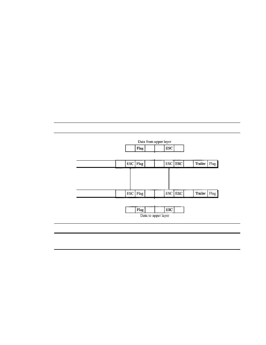
SECTION
11.1
FRAMING
309
character-oriented framing. In byte stuffing (or character stuffing), a special byte is
added to the data section of the frame when there is a character with the same pattern as
the flag. The data section is stuffed with an extra byte. This byte is usually called the
escape character (ESC),
which has a predefined bit pattern. Whenever the receiver
encounters the ESC character, it removes it from the data section and treats the next
character as data, not a delimiting flag.
Byte stuffing by the escape character allows the presence of the flag in the data sec-
tion of the frame, but it creates another problem. What happens if the text contains one or
more escape characters followed by a flag? The receiver removes the escape character,
but keeps the flag, which is incorrectly interpreted as the end of the frame. To solve this
problem, the escape characters that are part of the text must also be marked by another
escape character. In other words, if the escape character is part of the text, an extra one is
added to show that the second one is part of the text. Figure 11.2 shows the situation.
Figure 11.2
Byte stuffing and unstuffing
Frame sent
Flag
Header
Stuffed
Extra 2
bytes
Frame received
Flag
Header
Unstuffed
Byte stuffing is the process of adding 1 extra byte whenever
there is a flag or escape character in the text.
Character-oriented protocols present another problem in data communications.
The universal coding systems in use today, such as Unicode, have 16-bit and 32-bit
characters that conflict with 8-bit characters. We can say that in general, the tendency is
moving toward the bit-oriented protocols that we discuss next.
Bit-Oriented Protocols
In a
bit-oriented protocol,
the data section of a frame is a sequence of bits to be inter-
preted by the upper layer as text, graphic, audio, video, and so on. However, in addition
to headers (and possible trailers), we still need a delimiter to separate one frame from
the other. Most protocols use a special 8-bit pattern flag 01111110 as the delimiter to
define the beginning and the end of the frame, as shown in Figure 11.3.
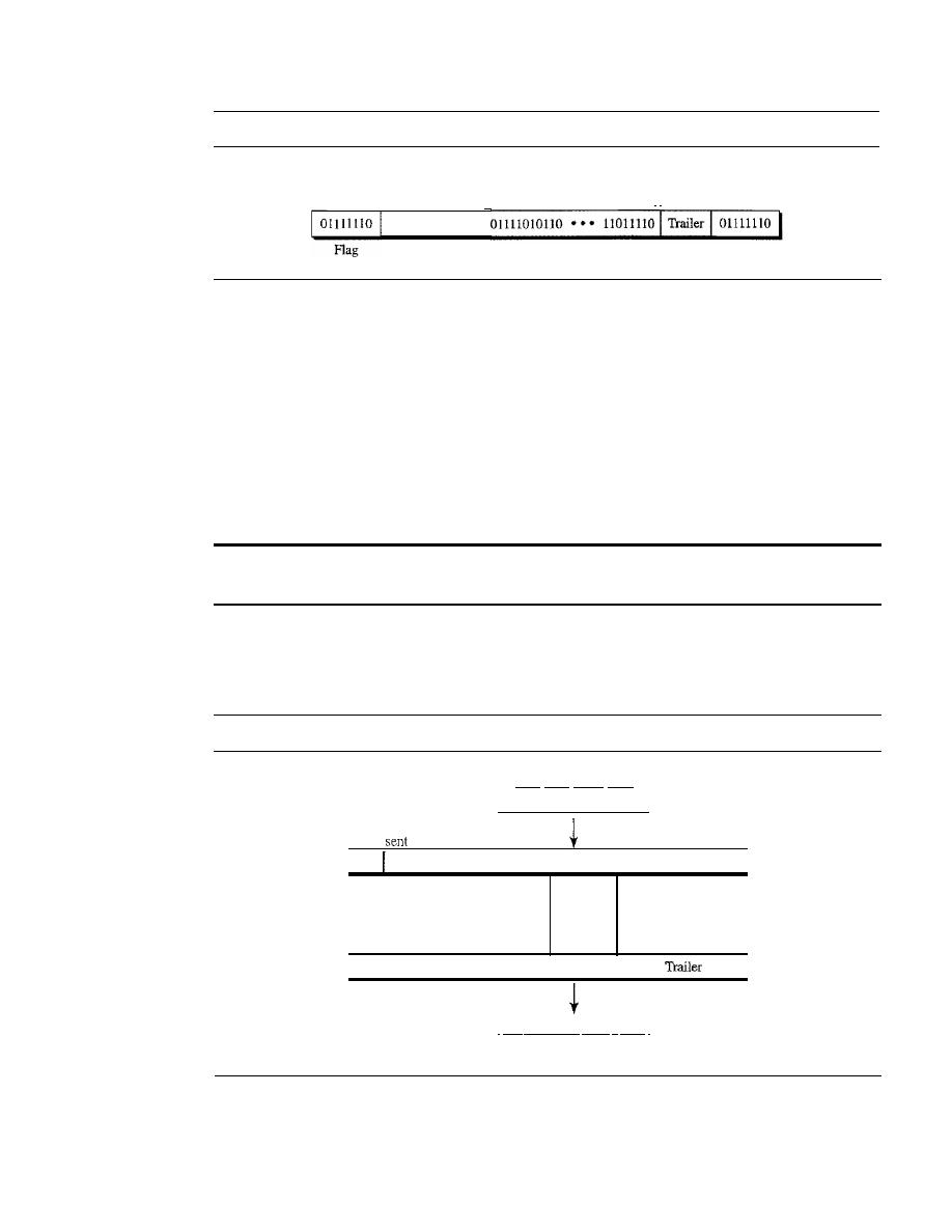
310
CHAPTER
11
DATA LINK CONTROL
Figure 11.3
A frame in a bit-oriented protocol
I'
Data from upper layer
Variable number of bits
'
I
Header
Flag
This flag can create the same type of problem we saw in the byte-oriented proto-
cols. That is, if the flag pattern appears in the data, we need to somehow inform the
receiver that this is not the end of the frame. We do this by stuffing 1 single bit (instead
of I byte) to prevent the pattern from looking like a flag. The strategy is called
bit
stuffing.
In bit stuffing, if a 0 and five consecutive I bits are encountered, an extra 0 is
added. This extra stuffed bit is eventually removed from the data by the receiver. Note
that the extra bit is added after one 0 followed by five 1s regardless of the value of the
next bit. This guarantees that the flag field sequence does not inadvertently appear in
the frame.
Bit stuffing is the process of adding one extra 0 whenever five consecutive 18 follow a 0
in the data, so that the receiver does not mistake the pattern 0111110 for a flag.
Figure 11.4 shows bit stuffing at the sender and bit removal at the receiver. Note that
even if we have a 0 after five 1s, we still stuff a O. The 0 will be removed by the receiver.
Figure 11.4
Bit stuffing and unstuffing
Frame
I
Flag
Header
Frame received
Data from upper layer
100011111110011111010001
Stuffed
10001111101100111110010001 Trailer
I
Flag
I
Extra
2
bits
I
Flag
1
Header
10001111101100111110010001
1Flag
I
Unsroffed
I
000 1l11l1100111110 1000
I
Data to upper layer
This means that if the flaglike pattern 01111110 appears in the data, it will change
to 011111010 (stuffed) and is not mistaken as a flag by the receiver. The real flag 01111110
is not stuffed by the sender and is recognized by the receiver.

SECTION II.3
PROTOCOLS
311
11.2
FLOW AND ERROR CONTROL
Data communication requires at least two devices working together, one to send and the
other to receive. Even such a basic arrangement requires a great deal of coordination
for an intelligible exchange to occur. The most important responsibilities of the data
link layer are flow control and error control. Collectively, these functions are known
as data link control.
Flow Control
Flow control coordinates the amount of data that can be sent before receiving an acknowl-
edgment and is one of the most important duties of the data link layer. In most protocols,
flow control is a set of procedures that tells the sender how much data it can transmit
before it must wait for an acknowledgment from the receiver. The flow of data must not
be allowed to overwhelm the receiver. Any receiving device has a limited speed at which
it can process incoming data and a limited amount of memory in which to store incom-
ing data. The receiving device must be able to inform the sending device before those
limits are reached and to request that the transmitting device send fewer frames or stop
temporarily. Incoming data must be checked and processed before they can be used. The
rate of such processing is often slower than the rate of transmission. For this reason,
each receiving device has a block of memory, called a
buffer,
reserved for storing incom-
ing data until they are processed. If the buffer begins to fill up, the receiver must be able
to tell the sender to halt transmission until it is once again able to receive.
Flow control refers to a set of procedures used to restrict the amount of data
that the sender can send before waiting for acknowledgment.
Error Control
Error control is both error detection and error correction.
It
allows the receiver to
inform the sender of any frames lost or damaged in transmission and coordinates the
retransmission of those frames by the sender. In the data link layer, the term error con-
trol refers primarily to methods of error detection and retransmission. Error control in
the data link layer is often implemented simply: Any time an error is detected in an
exchange, specified frames are retransmitted. This process is called automatic repeat
request (ARQ).
Error control in the data link layer is based on automatic
repeat request, which is the retransmission of data.
11.3
PROTOCOLS
Now let us see how the data link layer can combine framing, flow control, and error control
to achieve the delivery of data from one node to another. The protocols are normally imple-
mented in software by using one of the common programming languages. To make our
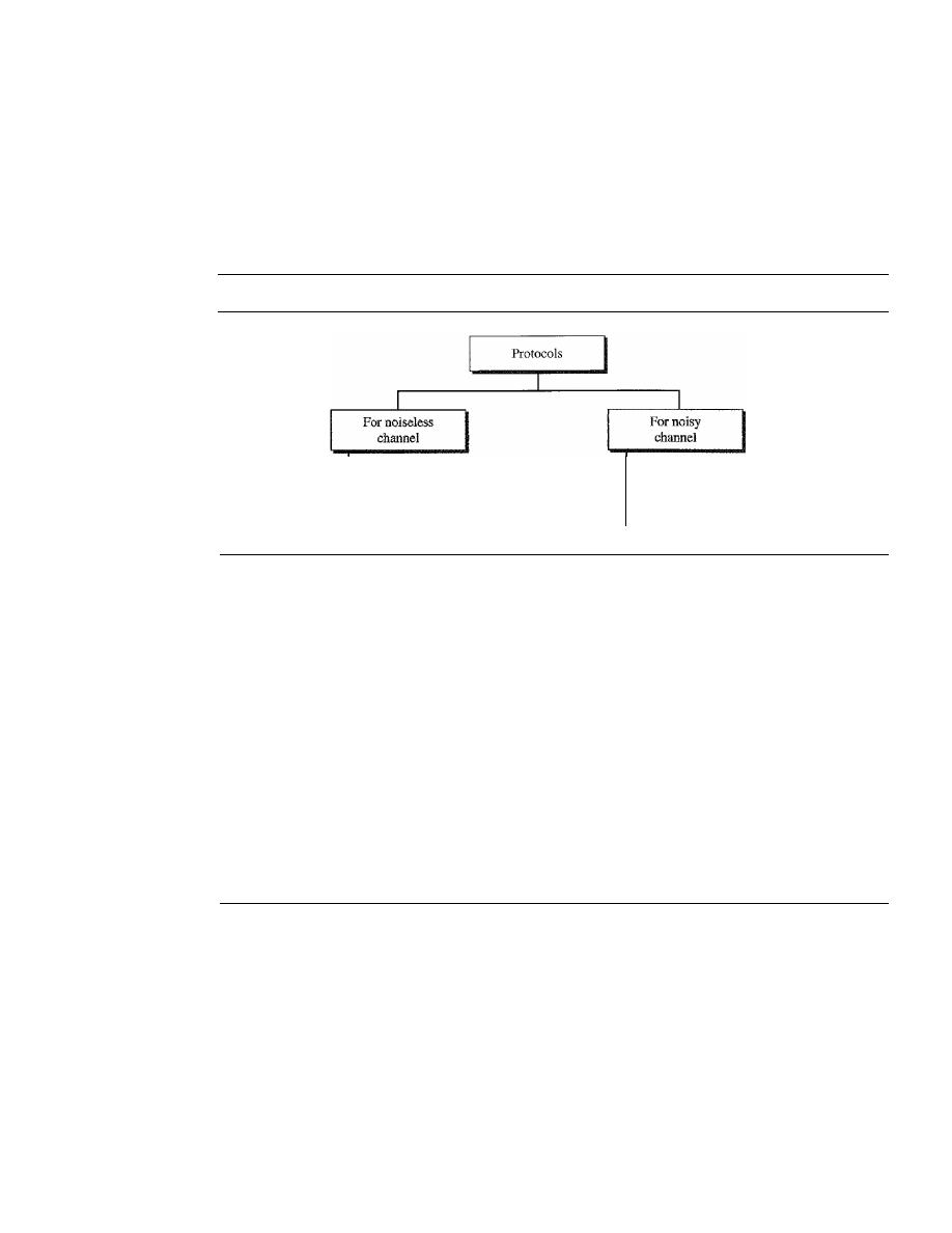
312
CHAPTER
11
DATA LINK CONTROL
discussions language-free, we have written in pseudocode a version of each protocol that
concentrates mostly on the procedure instead of delving into the details of language rules.
We divide the discussion of protocols into those that can be used for noiseless
(error-free) channels and those that can be used for noisy (error-creating) channels. The
protocols in the first category cannot be used in real life, but they serve as a basis for
understanding the protocols of noisy channels. Figure 11.5 shows the classifications.
Figure 11.5
Taxonomy ofprotocols discussed in this chapter
Simplest
Stop-and-Wait
Stop-and-Wait ARQ
Go-Hack-N ARQ
Selective Repeat ARQ
There is a difference between the protocols we discuss here and those used in real
networks. All the protocols we discuss are unidirectional in the sense that the data frames
travel from one node, called the sender, to another node, called the receiver. Although
special frames, called acknowledgment (ACK) and negative acknowledgment (NAK)
can flow in the opposite direction for flow and error control purposes, data flow in only
one direction.
In a real-life network, the data link protocols are implemented as bidirectional;
data flow in both directions. In these protocols the flow and error control information such
as ACKs and NAKs is included in the data frames in a technique called piggybacking.
Because bidirectional protocols are more complex than unidirectional ones, we chose the
latter for our discussion. If they are understood, they can be extended to bidirectional
protocols. We leave this extension as an exercise.
11.4
NOISELESS CHANNELS
Let us first assume we have an ideal channel in which no frames are lost, duplicated, or
corrupted. We introduce two protocols for this type of channel. The first is a protocol
that does not use flow control; the second is the one that does. Of course, neither has error
control because we have assumed that the channel is a perfect noiseless channel.
Simplest Protocol
Our first protocol, which we call the Simplest Protocol for lack of any other name, is one
that has no flow or en'or control. Like other protocols we will discuss in this chapter, it is a
unidirectional protocol in which data frames are traveling in only one direction-from the
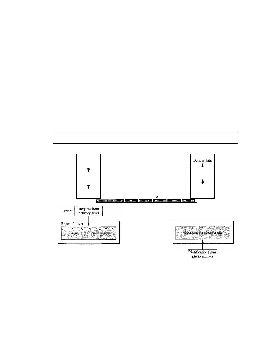
SECTION
11.4
NOISELESS CHANNELS
313
sender to receiver. We assume that the receiver can immediately handle any frame it
receives with a processing time that is small enough to be negligible. The data link
layer of the receiver immediately removes the header from the frame and hands the data
packet to its network layer, which can also accept the packet immediately. In other
words, the receiver can never be overwhelmed with incoming frames.
Design
There is no need for flow control in this scheme. The data link layer at the sender site
gets data from its network layer, makes a frame out of the data, and sends it. The data
link layer at the receiver site receives a frame from its physical layer, extracts data from
the frame, and delivers the data to its network layer. The data link layers of the sender
and receiver provide transmission services for their network layers. The data link layers
use the services provided by their physical layers (such as signaling, multiplexing, and
so on) for the physical transmission of bits. Figure 11.6 shows a design.
Figure 11.6
The design of the simplest protocol with no flow or error control
Sender
Receiver
Network
Data link
Physical
Get data
I
I
I
Send frame
Receive frame
Data frames
I
I
Network
Data link
Physical
Repeat forever
Event:
We need to elaborate on the procedure used by both data link layers. The sender site
cannot send a frame until its network layer has a data packet to send. The receiver site
cannot deliver a data packet to its network layer until a frame arrives.
If
the protocol is
implemented as a procedure, we need to introduce the idea of events in the protocol. The
procedure at the sender site is constantly running; there is no action until there is a request
from the network layer. The procedure at the receiver site is also constantly rulming, but
there is no action until notification from the physical layer arrives. Both procedures are
constantly running because they do not know when the corresponding events will occur.
314
CHAPTER
11
DATA LINK CONTROL
Algorithms
Algorithm 11.1 shows the procedure at the sender site.
Algorithm 11.1
Sender-site algorithm for the simplest protocol
//Send the frame
II
Sleep until an event occurs
//There is
packet
to send
GetData()i
MakeFrame()i
SendFrame()i
}
WaitForEvent()i
if(Event(RequestToSend»
{
1 while (true)
II
Repeat forever
2
{
3
4
5
6
7
8
9
10
}
Analysis
The algorithm has an infinite loop, which means lines
3
to
9
are repeated forever
once the program starts. The algorithm is an event-driven one, which means that it
sleeps
(line 3)
until an event
wakes
it
up
(line 4). This means that there may be an undefined span of time
between the execution of line 3 and line 4; there is a gap between these actions. When the event,
a request from the network layer, occurs, lines 6 though 8 are executed. The program then repeats
the loop and again sleeps at line 3 until the next occurrence of the event. We have written
pseudocode for the main process. We do not show any details for the modules GetData, Make-
Frame, and SendFrame. GetDataO takes a data packet from the network layer, MakeFrameO adds
a header and delimiter flags to the data packet to make a frame, and SendFrameO delivers the
frame to the physical layer for transmission.
Algorithm 11.2 shows the procedure at the receiver site.
Algorithm 11.2
Receiver-site algorithm for the simplest protocol
/ /Deli ver data
to
network layez
ReceiveFrame()i
ExtractData()i
Del ive rDat a ( )
i
}
1 while(true)
II
Repeat forever
2
{
3
WaitForEvent()i
II
Sleep until an event
4
if(Event(ArrivalNotification»
IIData frame arrived
5
{
6
7
8
9
10
}
Analysis
This algorithm has the same format as Algorithm 11.1, except that the direction of
the frames and data is upward. The event here is the arrival of a data frame. After the event
occurs, the data link layer receives the frame from the physical layer using the ReceiveFrameO
process, extracts the data from the frame using the ExtractDataO process, and delivers the data to
the network layer using the DeliverDataO process. Here, we also have an event-driven algorithm
because the algorithm never knows when the data frame will arrive.
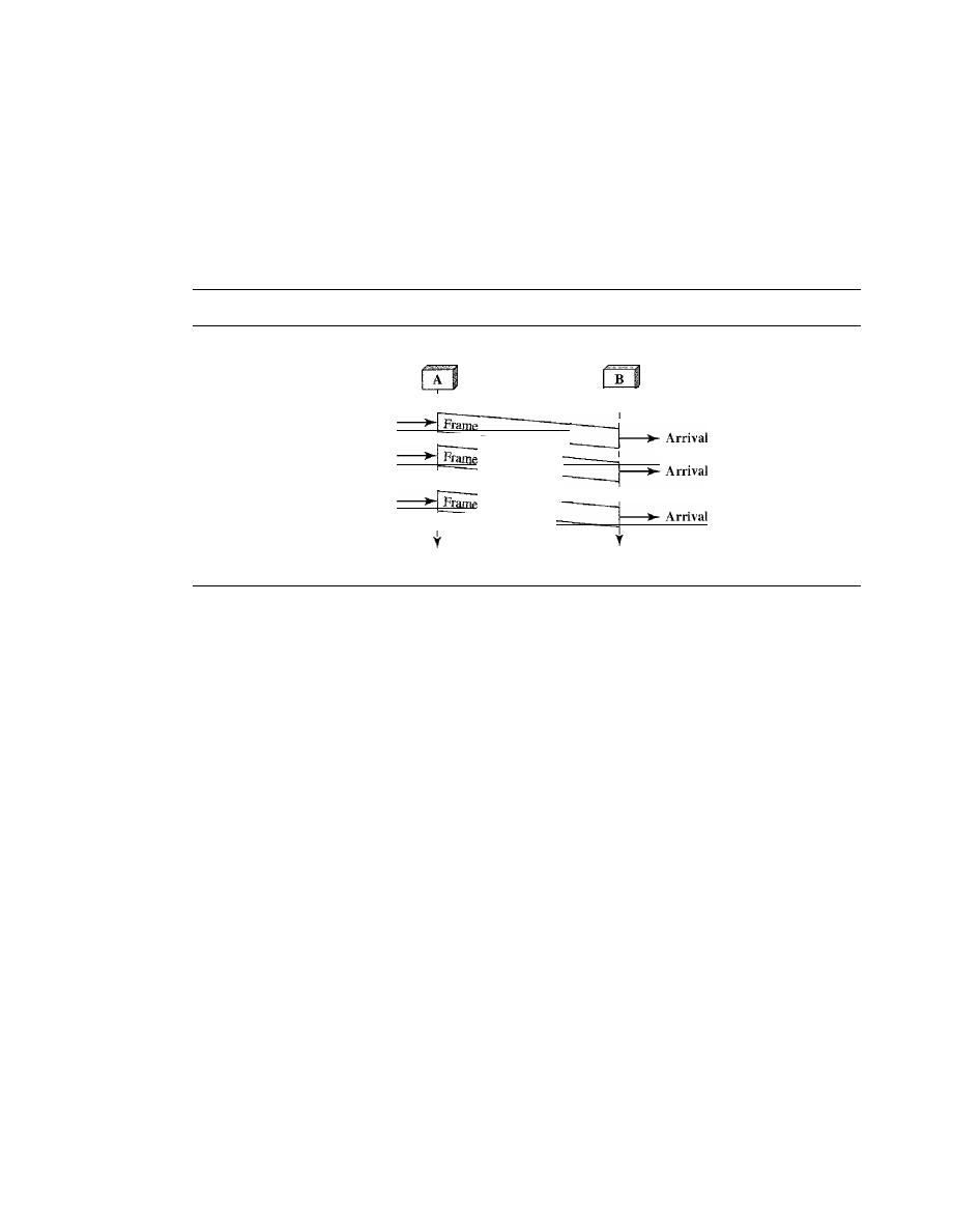
SECTION
11.4
NOISELESS CHANNELS
315
Example 11.1
Figure 11.7 shows an example of communication using this protocol.
It
is very simple. The
sender sends a sequence of frames without even thinking about the receiver. To send three frames,
three events occur at the sender site and three events at the receiver site. Note that the data frames
are shown by tilted boxes; the height of the box defines the transmission time difference between
the first bit and the last bit in the frame.
Figure 11.7
Flow diagram for Example 11.1
Sender
Receiver
I
I
I
I
Request
I
Request
:
Request
:
:
Time
Time
Stop-and-Wait Protocol
If data frames arrive at the receiver site faster than they can be processed, the frames
must be stored until their use. Normally, the receiver does not have enough storage
space, especially if it is receiving data from many sources. This may result in either the
discarding of frames or denial of service. To prevent the receiver from becoming over-
whelmed with frames,we somehow need to tell the sender to slow down. There must be
feedback from the receiver to the sender.
The protocol we discuss now is called the
Stop-and-Wait Protocol
because the
sender sends one frame, stops until it receives confirmation from the receiver (okay to
go ahead), and then sends the next frame. We still have unidirectional communication
for data frames, but auxiliary ACK frames (simple tokens of acknowledgment) travel
from the other direction. We add flow control to our previous protocol.
Design
Figure 11.8 illustrates the mechanism. Comparing this figure with Figure 11.6, we can
see the traffic on the forward channel (from sender to receiver) and the reverse channel.
At any time, there is either one data frame on the forward channel or one ACK frame on
the reverse channel. We therefore need a half-duplex link.
Algorithms
Algorithm 11.3 is for the sender site.
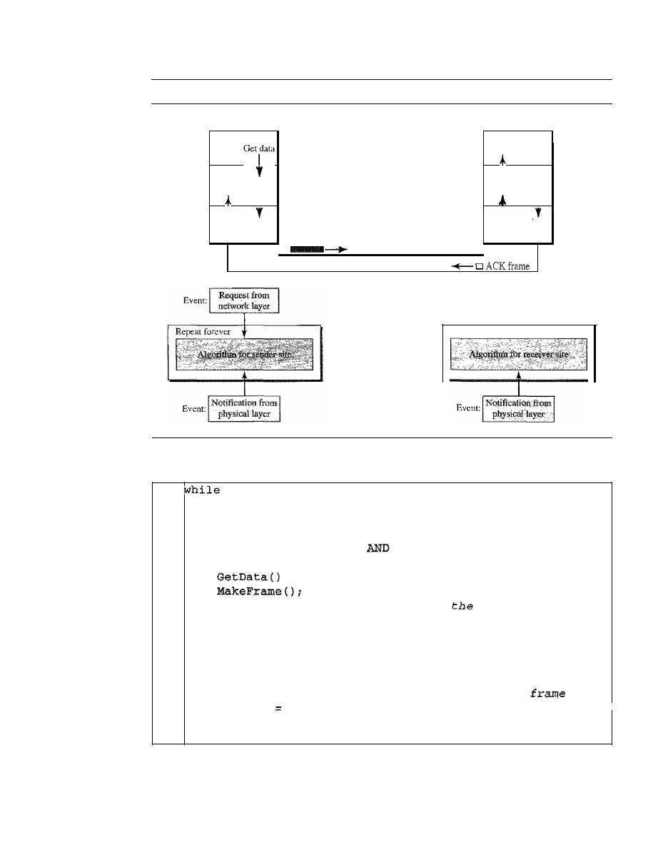
316
CHAPTER
11
DATA LINK CONTROL
Figure 11.8
Design of Stop-and- Wait Protocol
Sender
Receiver
Network
Data link:
Physical
Deliver
data
I
I
I
R
I.
R
I.
ecelve Send
ecelVe
Send
frame
frame
frame
frame
Data frame
I
I
Network
Data link
Physical
Repeat forever
Algorithm 11.3
Sender-site algorithm for Stop-and- Wait Protocol
(true)
canS end
=
true
II
Sleep until an event occurs
canSend}
II
Sleep until an event occurs
/1
An ACK has arrived
I/Send
data frame
I/cannot send until ACK arrives
IIRepeat
forever
IIAllow
the first frame to go
I/Receive the ACK
ReceiveFrame();
canSend
true;
i
SendFrame()i
canSend
=
false;
}
}
WaitForEvent()i
if (Event (ArrivalNotification)
{
{
WaitForEvent()i
if (Event (RequestToSend)
{
1
2
3
4
5
6
7
8
9
10
11
12
13
14
15
16
17
18
}
Analysis
Here two events can occur: a request from the network layer or an arrival notifica-
tion from the physical layer. The responses to these events must alternate. In other words, after a
frame is sent, the algorithm must ignore another network layer request until that frame is
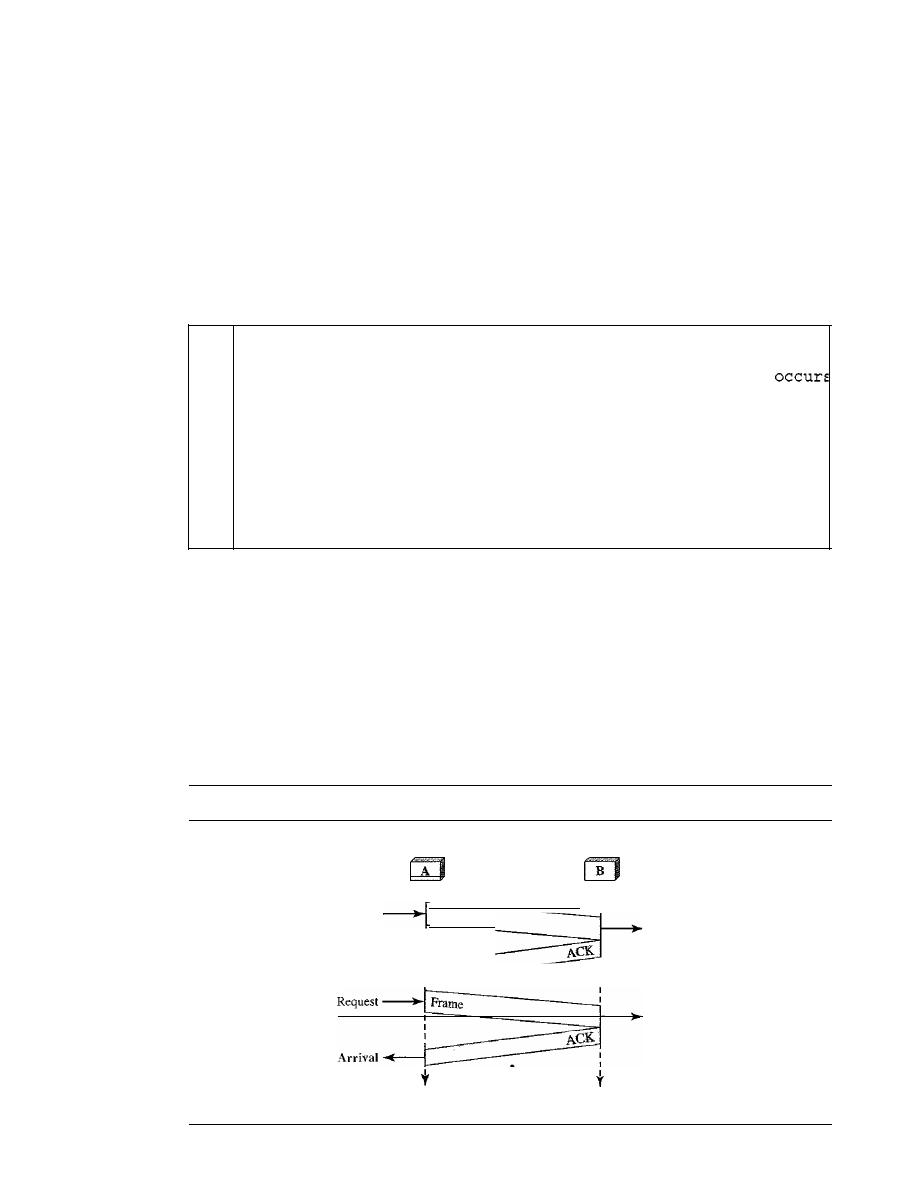
SECTION 1I.4
NOISELESS CHANNELS
317
acknowledged. We know that two arrival events cannot happen one after another because the
channel is error-free and does not duplicate the frames. The requests from the network layer,
however, may happen one after another without an arrival event in between. We need somehow to
prevent the immediate sending of the data frame. Although there are several methods, we have
used a simple canSend variable that can either be true or false. When a frame is sent, the variable
is set to false to indicate that a new network request cannot be sent until canSend is true. When an
ACK is received, canSend is set to true to allow the sending of the next frame.
Algorithm 11.4 shows the procedure at the receiver site.
Algorithm 11.4
Receiver-site algorithm for Stop-and- Wait Protocol
WaitForEvent();
II
Sleep until an event
if(Event(ArrivalNotification)}
IIData frame arrives
{
/IDeliver data to network
layex
IISend an
ACK
frame
IIRepeat forever
ReceiveFrame(};
ExtractData(}i
Deliver(data};
SendFrame();
}
1
while (true)
2
{
3
4
5
6
7
8
9
10
11
}
Analysis
This is very similar to Algorithm 11.2 with one exception. After the data frame
arrives, the receiver sends an ACK frame (line 9) to acknowledge the receipt and allow the sender
to send the next frame.
Example 11.2
Figure 11.9 shows an example of communication using this protocol.
It
is still very simple. The
sender sends one frame and waits for feedback from the receiver. When the ACK arrives, the
sender sends the next frame. Note that sending two frames in the protocol involves the sender in
four events and the receiver in two events.
Figure 11.9
Flow diagramfor Example 1I.2
Sender
Receiver
Arrival
Frame
Arrival
:
I
Request
:
I
Arrival
I
A r r i v a l '
I
•
1
Time
Time

318
CHAPTER
11
DATA LINK CONTROL
11.5
NOISY CHANNELS
Although the Stop-and-Wait Protocol gives us an idea of how to add flow control to its
predecessor, noiseless channels are nonexistent. We can ignore the error (as we some-
times do), or we need to add error control to our protocols. We discuss three protocols
in this section that use error control.
Stop-and-Wait Automatic Repeat Request
Our first protocol, called the
Stop-and-Wait Automatic Repeat Request (Stop-and-
Wait ARQ),
adds a simple error control mechanism to the Stop-and-Wait Protocol. Let
us see how this protocol detects and corrects errors.
To detect and correct corrupted frames, we need to add redundancy bits to our data
frame (see Chapter 10). When the frame arrives at the receiver site, it is checked and if
it is corrupted, it is silently discarded. The detection of errors in this protocol is mani-
fested by the silence of the receiver.
Lost frames are more difficult to handle than corrupted ones. In our previous proto-
cols, there was no way to identify a frame. The received frame could be the correct one,
or a duplicate, or a frame out of order. The solution is to number the frames. When the
receiver receives a data frame that is out of order, this means that frames were either
lost or duplicated.
The comlpted and lost frames need to be resent in this protocol. If the receiver does
not respond when there is an error, how can the sender know which frame to resend? To
remedy this problem, the sender keeps a copy of the sent frame. At the same time, it starts
a timer.
If
the timer expires and there is no ACK for the sent frame, the frame is resent, the
copy is held, and the timer is restarted. Since the protocol uses the stop-and-wait mecha-
nism, there is only one specific frame that needs an ACK even though several copies of
the same frame can be in the network.
Error correction in Stop-and-Wait ARQ is done by keeping a copy of the sent frame
and retransmitting of the frame when the timer expires.
Since an ACK frame can also be corrupted and lost, it too needs redundancy bits
and a sequence number. The ACK frame for this protocol has a sequence number field.
In this protocol, the sender simply discards a corrupted ACK frame or ignores an
out-of-order one.
Sequence Numbers
As we discussed, the protocol specifies that frames need to be numbered. This is done
by using
sequence numbers.
A field is added to the data frame to hold the sequence
number of that frame.
One important consideration is the range of the sequence numbers. Since we want
to minimize the frame size, we look for the smallest range that provides unambiguous

SECTION
11.5
NOISY CHANNELS
319
communication. The sequence numbers of course can wrap around. For example, if we
decide that the field is
m bits long, the sequence numbers start from 0, go to
2
m
-
1, and
then are repeated.
Let us reason out the range of sequence numbers we need. Assume we have used
x
as
a sequence number; we only need to use
x
+
1 after that. There is no need for
x
+
2. To
show this, assume that the sender has sent the frame numbered
x.
Three things can happen.
1. The frame arrives safe and sound at the receiver site; the receiver sends an acknowl-
edgment. The acknowledgment arrives at the sender site, causing the sender to send
the next frame numbered
x
+
1.
2. The frame arrives safe and sound at the receiver site; the receiver sends an acknowl-
edgment, but the acknowledgment is corrupted or lost. The sender resends the frame
(numbered
x)
after the time-out. Note that the frame here is a duplicate. The receiver
can recognize this fact because it expects frame
x
+
I but frame
x
was received.
3. The frame is corrupted or never arrives at the receiver site; the sender resends the
frame (numbered
x)
after the time-out.
We can see that there is a need for sequence numbers
x
and
x
+
I because the receiver
needs to distinguish between case 1 and case 2. But there is no need for a frame to be
numbered
x
+
2. In case 1, the frame can be numbered
x again because frames x and x
+
1
are acknowledged and there is no ambiguity at either site. In cases 2 and 3, the new frame
is
x
+
I, not
x
+
2. If only
x and x
+
1 are needed, we can let
x
=
0 and
x
+
I
== 1. This
means that the sequence is 0, I, 0, I, 0, and so on. Is this pattern familiar? This is modulo-2
arithmetic as we saw in Chapter 10.
In Stop-and-Wait
we use sequence numbers to number the frames.
The sequence numbers are based on modul0-2 arithmetic.
Acknowledgment Numbers
Since the sequence numbers must be suitable for both data frames and ACK frames, we
use this convention: The acknowledgment numbers always announce the sequence
number of the next frame expected by the receiver. For example, if frame 0 has arrived
safe and sound, the receiver sends an ACK frame with acknowledgment 1 (meaning
frame 1 is expected next). If frame 1 has arrived safe and sound, the receiver sends an
ACK frame with acknowledgment 0 (meaning frame 0 is expected).
In
the acknowledgment number always announces in
modul0-2 arithmetic the sequence number of the next frame expected.
Design
Figure 11.10 shows the design of the Stop-and-Wait ARQ Protocol. The sending device
keeps a copy of the last frame transmitted until it receives an acknowledgment for that
frame. A data frames uses a seqNo (sequence number); an ACK frame uses an ackNo
(acknowledgment number). The sender has a control variable, which we call
Sn
(sender,
next frame to send), that holds the sequence number for the next frame to be sent (0 or 1).
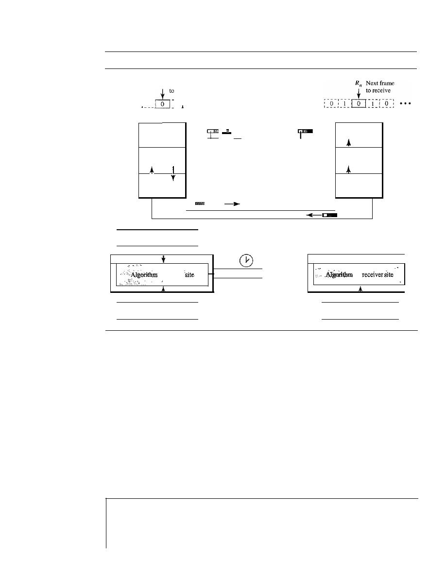
320
CHAPTER
11
DATA LINK CONTROL
Figure 11.10
Design of the Stop-and-WaitARQ Protocol
SII
Next frame
send
r---r---
---r---,
' 0 ' 1 0 1 ' 0 ' · · ·
L
_ __
J
Sender
Receiver
Network
Data link
Physical
Data frame
ACKframe
Deliver
-
Get data
data
I
seqNo
ackNo
T
I
I
R
I.
R
I.
T
ecelve Send
ecelve
Send
frame
frame
frame
frame
I
!
I
Network
Data link
Physical
Event:
I
Request from
I
network layer
I
Repeat forever
.
for sender
.-
Time-out
I
..
Event:
I
E
t:
I
Notification from
I
ven.
physical layer
Repeat forever
for
..
.
I
E
t:
I
Notification from
I
ven.
h ' all
P
ySlC
ayer
The receiver has a control variable, which we call
R
n
(receiver, next frame expected),
that holds the number of the next frame expected. When a frame is sent, the value of
Sn
is incremented (modulo-2), which means if it is 0, it becomes 1 and vice versa. When a
frame is received, the value of
R
n
is incremented (modulo-2), which means if it is 0, it
becomes 1 and vice versa. Three events can happen at the sender site; one event can
happen at the receiver site. Variable
Sn
points to the slot that matches the sequence
number of the frame that has been sent, but not acknowledged;
R
n
points to the slot that
matches the sequence number of the expected frame.
Algorithms
Algorithm 11.5 is for the sender site.
Algorithm 11.5
Sender-site algorithm for Stop-and- Wait ARQ
WaitForEvent();
1
n
=
0;
2
anSend
=
true;
3
hile (true)
4
{
5
II
Frame 0 should be sent first
II
Allow the first request to go
II
Repeat forever
II
Sleep until an event occurs

SECTION 11.5
NOISY CHANNELS
321
//Resend
a
copy check
//Copy is not needed
II
The timer expired
/ /The seqNo
Sn
//Keep copy
II
Sleep
II
An ACK has arrived
//Receive the ACE fram
/
/Valid ACK
Stoptimer{};
PurgeFrame(Sn_l);
canSend
=
true;
}
ReceiveFrame(ackNo);
if(not corrupted AND ackNo
{
}
Get Data ()
i
MakeFrame (Sn) ;
StoreFrame(Sn);
SendFrame(Sn) ;
StartTimerO;
Sn
=
Sn
+
1;
canSend
=
false;
if (Event (TimeOUt)
{
StartTimer();
ResendFrame(Sn_l);
}
}
WaitForEvent();
if (Event (ArrivaINotification)
{
Algorithm 11.5
Sender-site algorithm for Stop-and- Wait ARQ (continued)
6
if (Event (RequestToSend) AND canSend)
7
{
8
9
10
11
12
13
14
15
16
17
18
19
20
21
22
23
24
25
26
27
28
29
30
31
32
33
}
Analysis
We first notice the presence of
Sn'
the sequence number of the next frame to be sent.
This variable is initialized once (line 1), but it is incremented every time a frame is sent (line 13) in
preparation for the next frame. However, since this is modulo-2 arithmetic, the sequence numbers are
0, 1,0, 1, and so on. Note that the processes
in
the first event (SendFrame, StoreFrame, and Purge-
Frame) use an
Sn
defining the frame sent out. We need at least one buffer to hold this frame until
we are sure that it is received safe and sound. Line 10 shows that before the frame is sent, it is stored.
The copy is used for resending a corrupt or lost frame. We are still using the canSend variable to pre-
vent the network layer from making a request before the previous frame is received safe and sound. If
the frame is not corrupted and the ackNo of the ACK frame matches the sequence number of the next
frame to send, we stop the timer and purge the copy of the data frame we saved. Otherwise, we just
ignore this event and wait for the next event to happen. After each frame is sent, a timer is started.
When the timer expires (line 28), the frame is resent and the timer is restarted.
Algorithm 11.6 shows the procedure at the receiver site.
Algorithm 11.6
Receiver-site algorithm for Stop-and- Wait ARQ Protocol
1
=
0;
2
hile (true)
3
{
4
WaitForEvent();
II
Frame 0 expected to arrive firs
II
Sleep until an event occurs
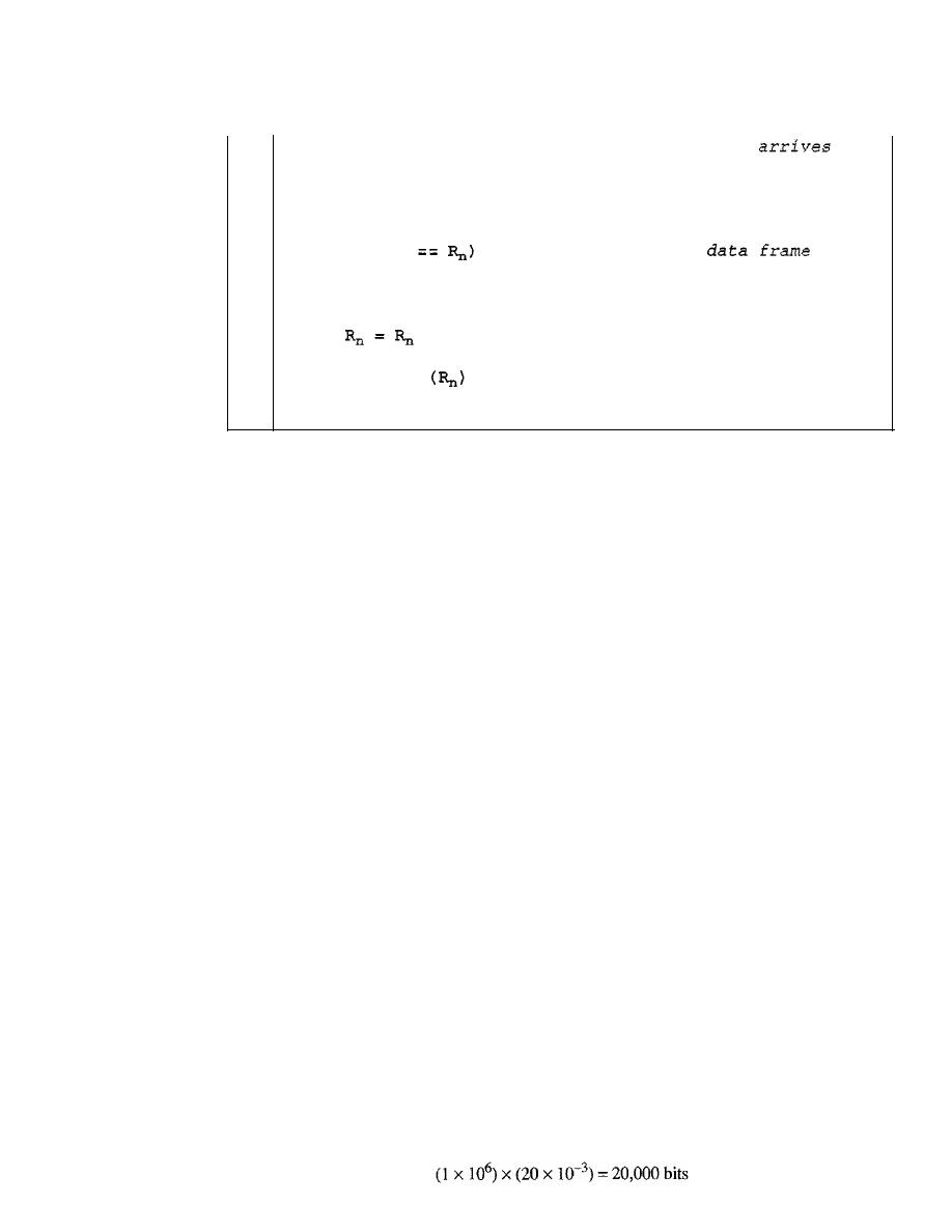
322
CHAPTER
11
DATA LINK CONTROL
Algorithm 11.6
Receiver-site algorithm for Stop-and- Wait ARQ Protocol (continued)
5
6
7
8
9
10
11
12
13
14
15
16
17
18
}
if(Event(Arriva1Notification»
{
ReceiveFrame()i
if(corrupted(frame»i
sleep ()
i
if (seqNo
{
ExtractData();
De1iverData()i
+
1;
}
SendFrame
;
}
//Data frame
//Valid
//Deliver
data
//Send
an ACK
Analysis
This is noticeably different from Algorithm 11.4. First, all arrived data frames that are
corrupted are ignored.
If
the seqNo of the frame is the one that is expected
(R
n ),
the frame is
accepted, the data are delivered to the network layer, and the value of R
n
is incremented. How-
ever, there is one subtle point here. Even if the sequence number of the data frame does not match
the next frame expected, an ACK is sent to the sender. This ACK, however, just reconfirms the
previous ACK instead of confirming the frame received. This is done because the receiver
assumes that the previous ACK might have been lost; the receiver is sending a duplicate frame.
The resent ACK may solve the problem before the time-out does it.
Example 11.3
Figure 11.11 shows an example of Stop-and-Wait ARQ. Frame
a
is sent and acknowledged.
Frame 1 is lost and resent after the time-out. The resent frame 1 is acknowledged and the timer
stops. Frame
a
is sent and acknowledged, but the acknowledgment is lost. The sender has no idea
if the frame or the acknowledgment is lost, so after the time-out, it resends frame 0, which is
acknowledged.
Efficiency
The Stop-and-WaitARQ discussed in the previous section is very inefficient if our chan-
nel is thick and long. By thick, we mean that our channel has a large bandwidth; by long,
we mean the round-trip delay is long. The product of these two is called the
bandwidth-
delay product,
as we discussed in Chapter
3.
We can think of the channel as a pipe. The
bandwidth-delay product then is the volume of the pipe in bits. The pipe is always there.
If
we do not use it, we are inefficient. The bandwidth-delay product is a measure of the
number of bits we can send out of our system while waiting for news from the receiver.
Example 11.4
Assume that, in a Stop-and-Wait ARQ system, the bandwidth of the line is 1 Mbps, and 1 bit
takes 20 ms to make a round trip. What is the bandwidth-delay product?
If
the system data frames
are 1000 bits in length, what is the utilization percentage of the link?
Solution
The bandwidth-delay product is
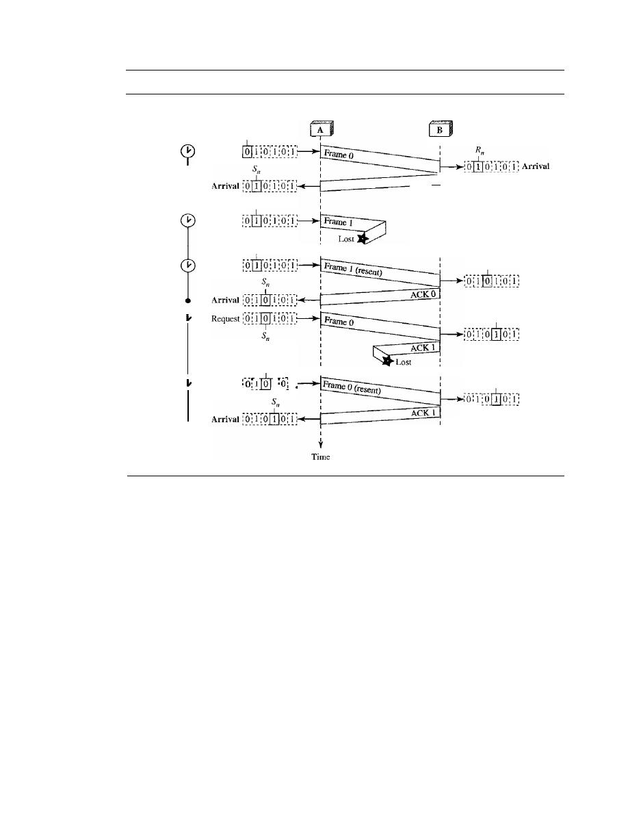
SECTION
11.5
NOISY CHANNELS
323
Figure 11.11
Flow diagram for Example 11.3
Sender
Receiver
R
n
Arrival
R
n
Arrival
R
n
Arrival
1 _ _ 1_ _
Discard, duplicate
I
I
I
ACK 1]
1
1
t
Time
5
n
Request
Sn
Request
5
n
Time-out
Stop
Start
Stop
l
Stop
Start
5"
Time-out
Time-out
i
f
"1-'
restart
,__
__ '__
__
Time-out
restart
The system can send 20,000 bits during the time it takes for the data to go from the sender to the
receiver and then back again. However, the system sends only 1000 bits. We can say that the link
utilization is only 1000/20,000, or 5 percent. For this reason, for a link with a high bandwidth or
long delay, the use of Stop-and-Wait ARQ wastes the capacity of the link.
Example 11.5
What is the utilization percentage of the link in Example 11.4 if we have a protocol that can send
up to 15 frames before stopping and worrying about the acknowledgments?
Solution
The bandwidth-delay product is still 20,000 bits. The system can send up to 15 frames or
15,000 bits during a round trip. This means the utilization is 15,000/20,000, or 75 percent. Of
course, if there are damaged frames, the utilization percentage is much less because frames
have to be resent.
Pipelining
In networking and in other areas, a task is often begun before the previous task has ended.
This is known as pipelining. There is no pipelining in Stop-and-Wait ARQ because we
need to wait for a frame to reach the destination and be acknowledged before the next
frame can be sent. However, pipelining does apply to our next two protocols because

324
CHAPTER
11
DATA LINK CONTROL
several frames can be sent before we receive news about the previous frames. Pipelining
improves the efficiency of the transmission if the number of bits in transition is large with
respect to the bandwidth-delay product.
Go-Back-N Automatic Repeat Request
To improve the efficiency of transmission (filling the pipe), multiple frames must be in
transition while waiting for acknowledgment. In other words, we need to let more than
one frame be outstanding to keep the channel busy while the sender is waiting for
acknowledgment.
In this section, we discuss one protocol that can achieve this goal; in
the next section, we discuss a second.
The first is called Go-Back-N Automatic Repeat Request (the rationale for the
name will become clear later). In this protocol we can send several frames before
receiving acknowledgments; we keep a copy of these frames until the acknowledg-
ments arrive.
Sequence Numbers
Frames from a sending station are numbered sequentially. However, because we need
to include the sequence number of each frame in the header, we need to set a limit.
If
the header of the frame allows
m bits for the sequence number, the sequence numbers
range from 0 to
2
m
-
1. For example, if
m is 4, the only sequence numbers are 0
through 15 inclusive. However, we can repeat the sequence. So the sequence num-
bers are
0, 1,2,3,4,5,6, 7,8,9, 10, 11, 12, 13, 14, 15,0, 1,2,3,4,5,6,7,8,9,10, 11, ...
In other words, the sequence numbers are modulo-2
m
.
In the Go-Back-N Protocol, the sequence numbers are modulo
where
m
is the size of the sequence number field in bits.
Sliding Window
In this protocol (and the next), the sliding window is an abstract concept that defines the
range of sequence numbers that is the concern of the sender and receiver. In other words,
the sender and receiver need to deal with only part of the possible sequence numbers. The
range which is the concern of the sender is called the send sliding window; the range that
is the concern of the receiver is called the receive sliding window. We discuss both here.
The send window is an imaginary box covering the sequence numbers of the data
frames which can be
in
transit. In each window position, some of these sequence numbers
define the frames that have been sent; others define those that can be sent. The maximum
size of the window is
2
m -
1 for reasons that we discuss later. In this chapter, we let the size
be fixed and set to the maximum value, but we will see in future chapters that some protocols
may have a variable window size. Figure 11.12 shows a sliding window of size 15
(m
=
4).
The window at any time divides the possible sequence numbers into four regions.
The first region, from the far left to the left wall of the window, defines the sequence
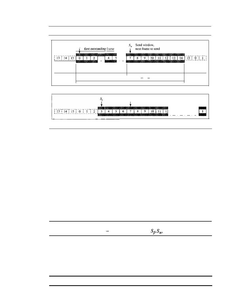
SECTION
11.5
NOISY CHANNELS
325
Figure 11.12
Send window for Go-Back-N ARQ
Sf
Send window,
3
!
6
Frames already
acknowledged
Frames sent, but not
acknowledged (outstanding)
Frames that can be sent,
but not received from upper layer
Frames that
cannot be sent
Send window, size
SSilC
2
m
1
a. Send window before sliding
5"
i
13
i
14
i
IS
i
0
b. Send window after sliding
numbers belonging to frames that are already acknowledged. The sender does not
worry about these frames and keeps no copies of them. The second region, colored in
Figure 11.12a, defines the range of sequence numbers belonging to the frames that are
sent and have an unknown status. The sender needs to wait to find out if these frames
have been received or were lost. We call these outstanding frames. The third range,
white in the figure, defines the range of sequence numbers for frames that can be sent;
however, the corresponding data packets have not yet been received from the network
layer. Finally, the fourth region defines sequence numbers that cannot be used until the
window slides, as we see next.
The window itself is an abstraction; three variables define its size and location at
any time. We call these variables
Sf(send
window, the first outstanding frame),
Sn
(send
window, the next frame to
be
sent), and
Ssize
(send window, size). The variable
Sf
defines
the sequence number of the first (oldest) outstanding frame. The variable
Sn
holds the
sequence number that will be assigned to the next frame to be sent. Finally, the variable
Ssize
defines the size of the window, which is fixed in our protocol.
The send window is an abstract concept defining an imaginary
box of size
2
m
1 with three variables:
and
Ssize'
Figure 11.12b shows how a send window can slide one or more slots to the right
when an acknowledgment arrives from the other end. As we will see shortly, the acknowl-
edgments in this protocol are cumulative, meaning that more than one frame can be
acknowledged by an ACK frame. In Figure 11.12b, frames 0, I, and 2 are acknowledged,
so the window has slid to the right three slots. Note that the value of
Sf
is 3 because frame 3
is now the first outstanding frame.
The send window can slide one or more slots when a valid acknowledgment arrives.
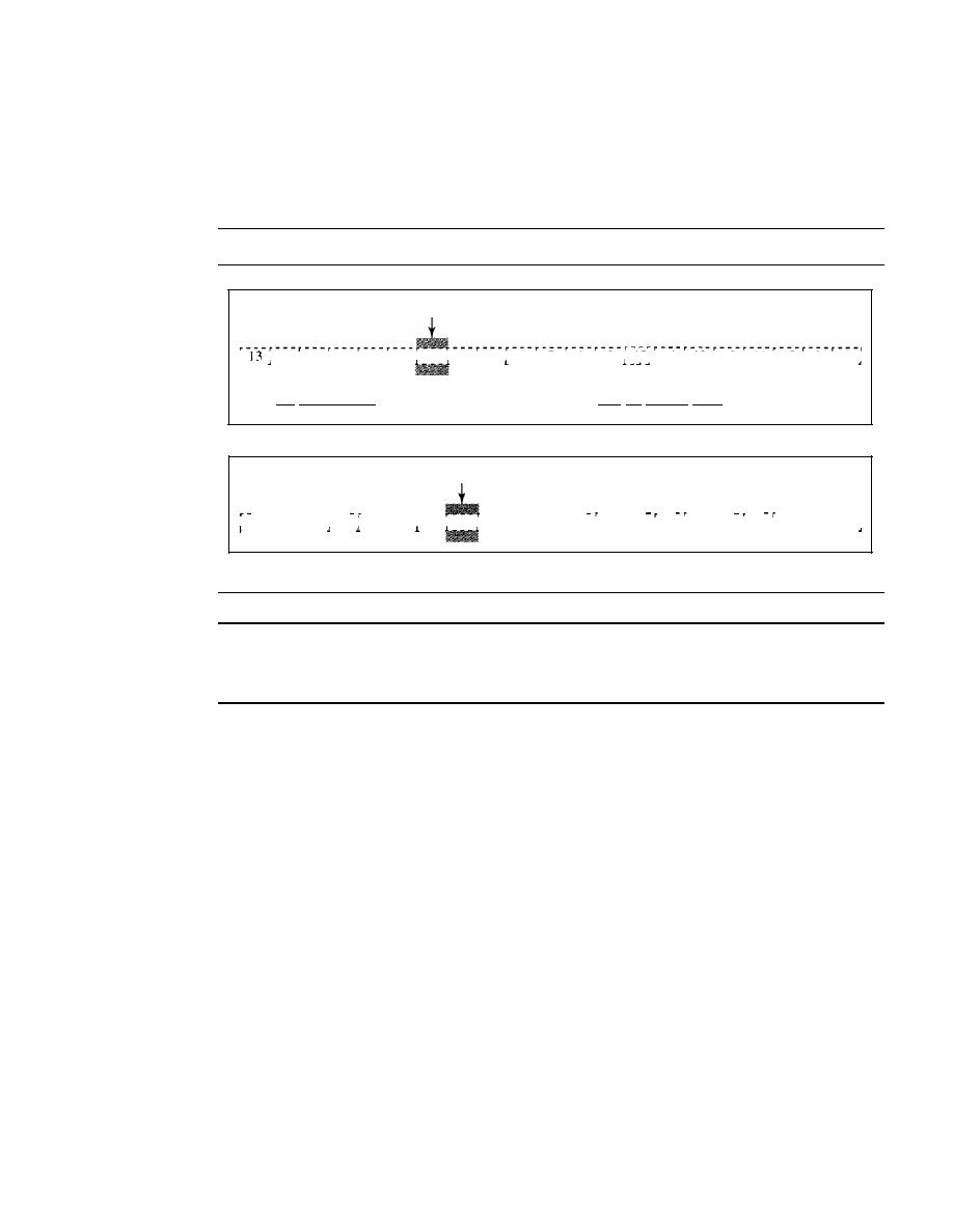
326
CHAPTER
11
DATA LINK CONTROL
The receive window makes sure that the correct data frames are received and that
the correct acknowledgments are sent. The size of the receive window is always I. The
receiver is always looking for the arrival of a specific frame. Any frame arriving out of
order is discarded and needs to be resent. Figure 11.13 shows the receive window.
Figure 11.13
Receive window for Go-Back-N ARQ
R
II
Receive window, next frame expected
,
I
14
I
IS
I
0
I
1
I
2 , 3
I
4
I
5
I
6
I
7
I
8 , 9
I
10
I
II , 12 , 13
I
14 , 15
I
0
I
1
I
l
J
l
l
1
J.
1
1
.1
1
1
1
.L
J
J
J
Frames already received
Frames that cannot be received
and acknowledged
until the window slides
a. Receive window
R
II
-
-,
- - -
,-
-
-,
- -
- --
,--
-
,-
- -
- -
-,
-
-
-,
-
--,
--
- -
-,
-- --
---,
- -
- -
- - -
,-
--,
-
--,
, 13
I
14
I
15
I
0
I
1
I
2
' 3 ' 4
I
5
I
6 ' 7
I
8 ' 9
I
10
I
I I
I
12
I
13 , 14
I
15
I
0
I
1 ,
J
J
1
.1.
1
.1
...
1
1
1
1
1
J.
.J
.I
b. Window after sliding
The receive window is an abstract concept defining an imaginary
box of size 1 with one single variable
R
n•
The window slides
when a correct frame has arrived; sliding occurs one slot at a time.
Note that we need only one variable R
n
(receive window, next frame expected) to
define this abstraction. The sequence numbers to the left of the window belong to the
frames already received and acknowledged; the sequence numbers to the right of this
window define the frames that cannot be received. Any received frame with a sequence
number in these two regions is discarded. Only a frame with a sequence number match-
ing the value of R
n
is accepted and acknowledged.
The receive window also slides, but only one slot at a time. When a correct frame
is received (and a frame is received only one at a time), the window slides.
Timers
Although there can be a timer for each frame that is sent, in our protocol we use only
one. The reason is that the timer for the first outstanding frame always expires first; we
send all outstanding frames when this timer expires.
Acknowledgment
The receiver sends a positive acknowledgment if a frame has arrived safe and sound
and in order.
If
a frame is damaged or is received out of order, the receiver is silent and
will discard all subsequent frames until it receives the one it is expecting. The silence of
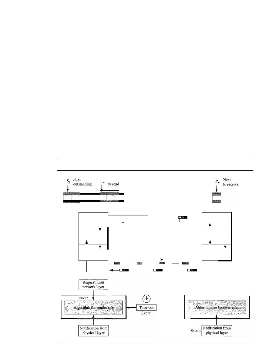
SECTION
11.5
NOISY CHANNELS
327
the receiver causes the timer of the unacknowledged frame at the sender site to expire.
This, in turn, causes the sender to go back and resend all frames, beginning with the one
with the expired timer. The receiver does not have to acknowledge each frame received.
It
can send one cumulative acknowledgment for several frames.
Resending a Frame
When the timer expires, the sender resends all outstanding frames. For example, suppose
the sender has already sent frame 6, but the timer for frame 3 expires. This means that
frame 3 has not been acknowledged; the sender goes back and sends frames 3, 4,5, and 6
again. That is why the protocol is called Go-Back-N ARQ.
Design
Figure 11.14 shows the design for this protocol. As we can see, multiple frames can
be in transit in the forward direction, and mUltiple acknowledgments in the reverse
direction. The idea is similar to Stop-and-Wait ARQ; the difference is that the send
Figure 11.14
Design of Go-Back-N ARQ
S
Next
I
i
I !
Sender
Receiver
Network
Data link
Physical
Data frame
ACKframe
Deliver
Get data
'1
data
I
seqNo
ackNo
I
I
I
R
I,
I,
ecelve Send
ReceIve
Send
frame
frame
frame
frame
I
i
,
!
w,
I
I
Network
Data link
Physical
Event:
Repeat forever
Event:
Repeat forever
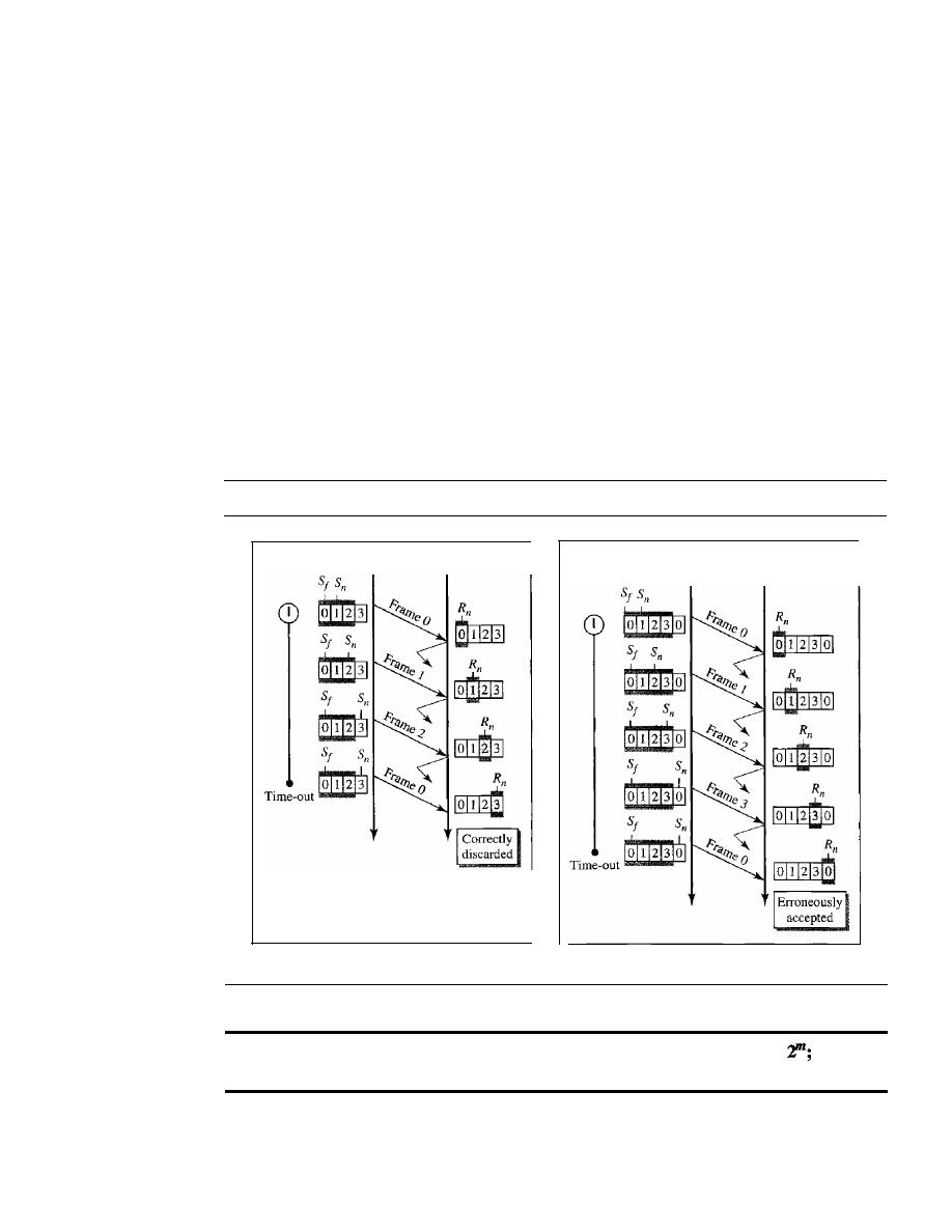
328
CHAPTER
11
DATA LINK CONTROL
window allows us to have as many frames in transition as there are slots in the send
window.
Send Window Size
We can now show why the size of the send window must be less than
2
m
.
As an
example, we choose
m
=
2, which means the size of the window can be
2
m
-
1, or 3.
Figure 11.15 compares a window size of 3 against a window size of 4.
If
the size of
the window is 3 (less than 2
2
)
and all three acknowledgments are lost, the frame
°
timer expires and all three frames are resent. The receiver is now expecting frame 3,
not frame 0, so the duplicate frame is correctly discarded. On the other hand, if the
size of the window is 4 (equal to 2
2
)
and all acknowledgments are lost, the sender
will send a duplicate of frame 0. However, this time the window of the receiver
expects to receive frame 0, so it accepts frame 0, not as a duplicate, but as the first
frame in the next cycle. This is an error.
Figure 11.15
Window size for Go-Back-N ARQ
Sender
Receiver
Sender
Receiver
a. Window size
<
2
m
b. Window size
=
2
m
In Go-Back-N ARQ, the size of the send window must be less than
the size of the receiver window is always 1.
Algorithms
Algorithm 11.7 shows the procedure for the sender in this protocol.

SECTION
11.5
NOISY CHANNELS
329
Algorithm
11.7
Go-Back-N sender algorithm
if{Event{ArrivalNotification»
IIACK arrives
{
(true)
{
WaitForEvent();
if(Event(RequestToSend»
{
if{Event{TimeOut»
{
StartTimer() ;
Temp
=
Sf;
while{Temp
<
Sn);
{
SendFrame(Sf);
Sf
=
Sf
+
1;
}
//A packet to send
//Repeat forever
II
I f window is full
liThe timer expires
IIIf
a valid
ACK
Receive (ACK) ;
if{corrupted{ACK»
Sleep ();
if{{ackNo>sf)&&{ackNO<=Sn»
While(Sf <= ackNo)
{
PurgeFrame{Sf);
Sf
=
Sf
+
1;
}
StopTimer();
if
(Sn-Sf
>=
Sw)
Sleep () ;
GetData() ;
MakeFrame (Sn) ;
StoreFrame (Sn) ;
SendFrame(Sn) ;
Sn
=
Sn
+
1;
if(timer not running)
StartTimer{);
}
}
}
1
Sw
=
-
1;
2 Sf
=
0;
3
Sn
=
OJ
4
5
6
7
8
9
10
11
12
13
14
15
16
17
18
19
20
21
22
23
24
25
26
27
28
29
30
31
32
33
34
35
36
37
38
39
40
41
42
43
44
45
}
Analysis
This algorithm first initializes three variables. Unlike Stop-and-Wait
ARQ,
this pro-
tocol allows several requests from the network layer without the need for other events to occur;
we just need to be sure that the window is not full (line 12). In our approach, if the window is full,
330
CHAPTER J 1
DATA LINK CONTROL
the request is just ignored and the network layer needs to try again. Some implementations use other
methods such as enabling or disabling the network layer. The handling of the arrival event is more
complex than in the previous protocol. If we receive a corrupted ACK, we ignore it. If the adeNa
belongs to one of the outstanding frames, we use a loop to purge the buffers and move the left wall
to the right. The time-out event is also more complex. We first start a new timer. We then resend all
outstanding frames.
Algorithm 11.8 is the procedure at the receiver site.
Algorithm 11.8
Go-Back-N receiver algorithm
if(Event{ArrivalNotification»
/Data frame arrives
(
WaitForEvent();
IIIf expected
frame
IIRepeat forever
IIDeliver data
IISlide window
DeliverData()i
=
+
1;
SendACK
;
}
Receive(Frame);
if(corrupted(Frame»
Sleep(};
if(seqNo
==
{
}
1
=
0;
2
3
(true)
4 {
5
6
7
8
9
10
11
12
13
14
15
16
17
18
19
}
Analysis
This algorithm is simple. We ignore a corrupt or out-of-order frame.
If
a frame
arrives with an expected sequence number, we deliver the data, update the value of
R
n,
and send
an ACK with the ackNa showing the next frame expected.
Example 11.6
Figure 11.16 shows an example of Go-Back
-N.
This is an example of a case where the forward
channel is reliable, but the reverse is not. No data frames are lost, but some ACKs are delayed and
one is lost. The example also shows how cumulative acknowledgments can help if acknowledgments
are delayed or lost.
After initialization, there are seven sender events. Request events are triggered by data
from the network layer; arrival events are triggered by acknowledgments from the physical
layer. There is no time-out event here because all outstanding frames are acknowledged
before the timer expires. Note that although ACK 2 is lost, ACK 3 serves as both ACK 2 and
ACK3.
There are four receiver events, all triggered by the arrival of frames from the physical
layer.
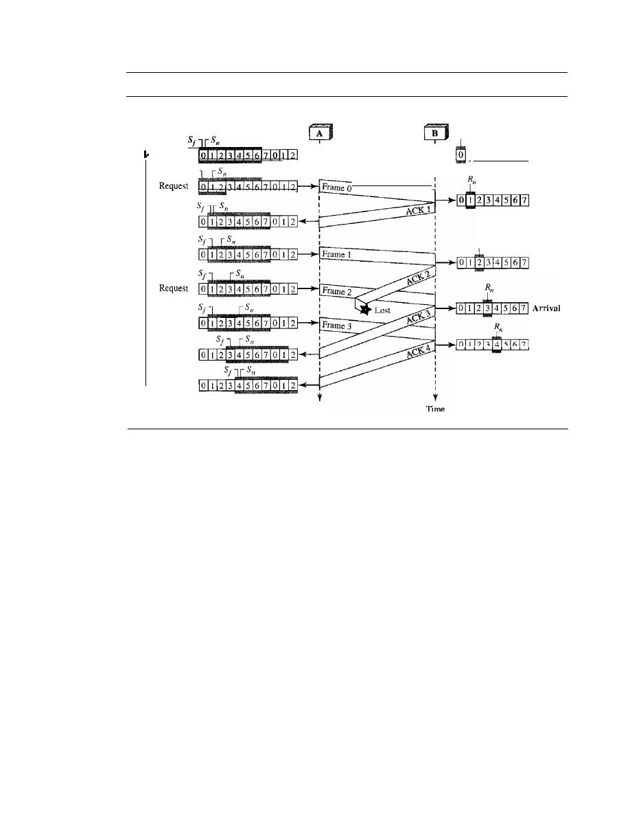
SECTION
11.5
NOISY CHANNELS
331
Figure 11.16
Flow diagram for Example 11.6
Arrival
Request
R
I1
Arrival
Receiver
R
I1
I
1213141516171
Initial
Arrival
Arrival
Time
Sender
Arrival
Arrival
Initial
Sf
Request
Start
timer
Stop
timer
Example 11.7
Figure 11.17 shows what happens when a frame is lost. Frames 0, 1, 2, and 3 are sent. However,
frame 1 is lost. The receiver receives frames 2 and 3, but they are discarded because they are
received out of order (frame 1 is expected). The sender receives no acknowledgment about
frames 1, 2, or 3. Its timer finally expires. The sender sends all outstanding frames
(1,
2, and 3)
because it does not know what is wrong. Note that the resending of frames l, 2, and 3 is the
response to one single event. When the sender is responding to this event, it cannot accept the
triggering of other events. This means that when ACK 2 arrives, the sender is still busy with send-
ing frame 3. The physica1layer must wait until this event is completed and the data link layer
goes back to its sleeping state. We have shown a vertical line to indicate the delay. It is the same
story with ACK 3; but when ACK 3 arrives, the sender is busy responding to ACK 2. It happens
again when ACK 4 arrives. Note that before the second timer expires, all outstanding frames have
been sent and the timer is stopped.
Go-Back-N ARQ Versus Stop-and- Wait ARQ
The reader may find that there is a similarity between
Go-Back-N ARQ and Stop-and-Wait
ARQ. We can say that the Stop-and-WaitARQ Protocol is actually a
Go-Back-N ARQ
in which there are only two sequence numbers and the send window size is 1. In other
words,
m
=
1,
2
m
-
1
=
1. In
Go-Back-N ARQ, we said that the addition is modulo-2
m
;
in
Stop-and-Wait ARQ it is 2, which is the same as
2
m
when
m
=
1.
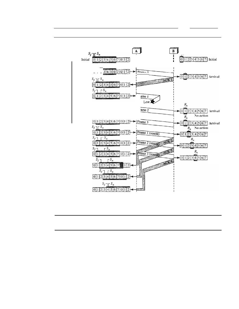
332
CHAPTER
11
DATA LINK CONTROL
Figure 11.17
Flow diagram for Example 11.7
Sender
Start
timer
Sf
Sn
Request
0 I 2 3 4 5 6 7 0 1
Receiver
R
n
I
I
R
n
Frame 0
I
Stop-and-WaitARQ is a special case of Go-Back-N ARQ
in which the size of the send window is 1.
Selective Repeat Automatic Repeat Request
Go-Back-N ARQ simplifies the process at the receiver site. The receiver keeps track of
only one variable, and there is no need to buffer out-of-order frames; they are simply
discarded. However, this protocol is very inefficient for a noisy link. In a noisy link a
frame has a higher probability of damage, which means the resending of multiple frames.
This resending uses up the bandwidth and slows down the transmission. For noisy links,
there is another mechanism that does not resend
N
frames when just one frame is dam-
aged; only the damaged frame is resent. This mechanism is called
Selective RepeatARQ.
It is more efficient for noisy links, but the processing at the receiver is more complex.
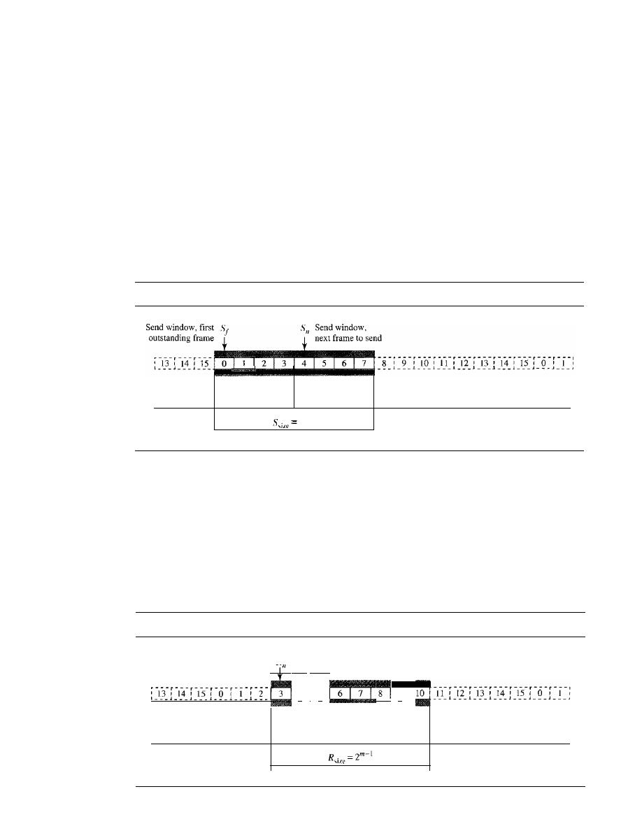
SECTION
11.5
NOISY CHANNELS
333
Windows
The Selective Repeat Protocol also uses two windows: a send window and a receive win-
dow. However, there are differences between the windows in this protocol and the ones in
Go-Back-N. First, the size of the send window is much smaller; it is 2
m
-
I
.
The reason for
this will be discussed later. Second, the receive window is the same size as the send window.
The send window maximum size can be
2
m
-
I
.
For example, if m
=
4, the
sequence numbers go from 0 to 15, but the size of the window is just 8 (it is 15 in
the Go-Back-N Protocol). The smaller window size means less efficiency in filling the
pipe, but the fact that there are fewer duplicate frames can compensate for this.
The protocol uses the same variables as we discussed for Go-Back-N. We show the
Selective Repeat send window in Figure 11.18 to emphasize the size. Compare it with
Figure 11.12.
Figure 11.18
Send window for Selective Repeat ARQ
L _ _ _
___
J _ _ _
_ _ _ 1 _ _ _ 1 _ _ _ 1 _ _ _ 1 _ _ _
_ _ _
_ _ _
J ___
J _ _ _
Frames already
Frames sent, but
Frames that can
Frames that
acknowledged
not acknowledged
be sent
cannot be sent
2
m
-
1
The receive window in Selective Repeat is totally different from the one in Go-
Back-N. First, the size of the receive window is the same as the size of the send window
(2
m
-
I
).
The Selective Repeat Protocol allows as many frames as the size of the receive
window to arrive out of order and be kept until there is a set of in-order frames to be
delivered to the network layer. Because the sizes of the send window and receive win-
dow are the same, all the frames in the send frame can arrive out of order and be stored
until they can be delivered. We need, however, to mention that the receiver never delivers
packets out of order to the network layer. Figure 11.19 shows the receive window in this
Figure 11.19
Receive window for Selective Repeat ARQ
R
Receive window•
next frame expected
4
!
5
9
Frames that can be received
Frames already
and stored for later delivery.
received
Colored boxes, already received
Frames that
cannot be received
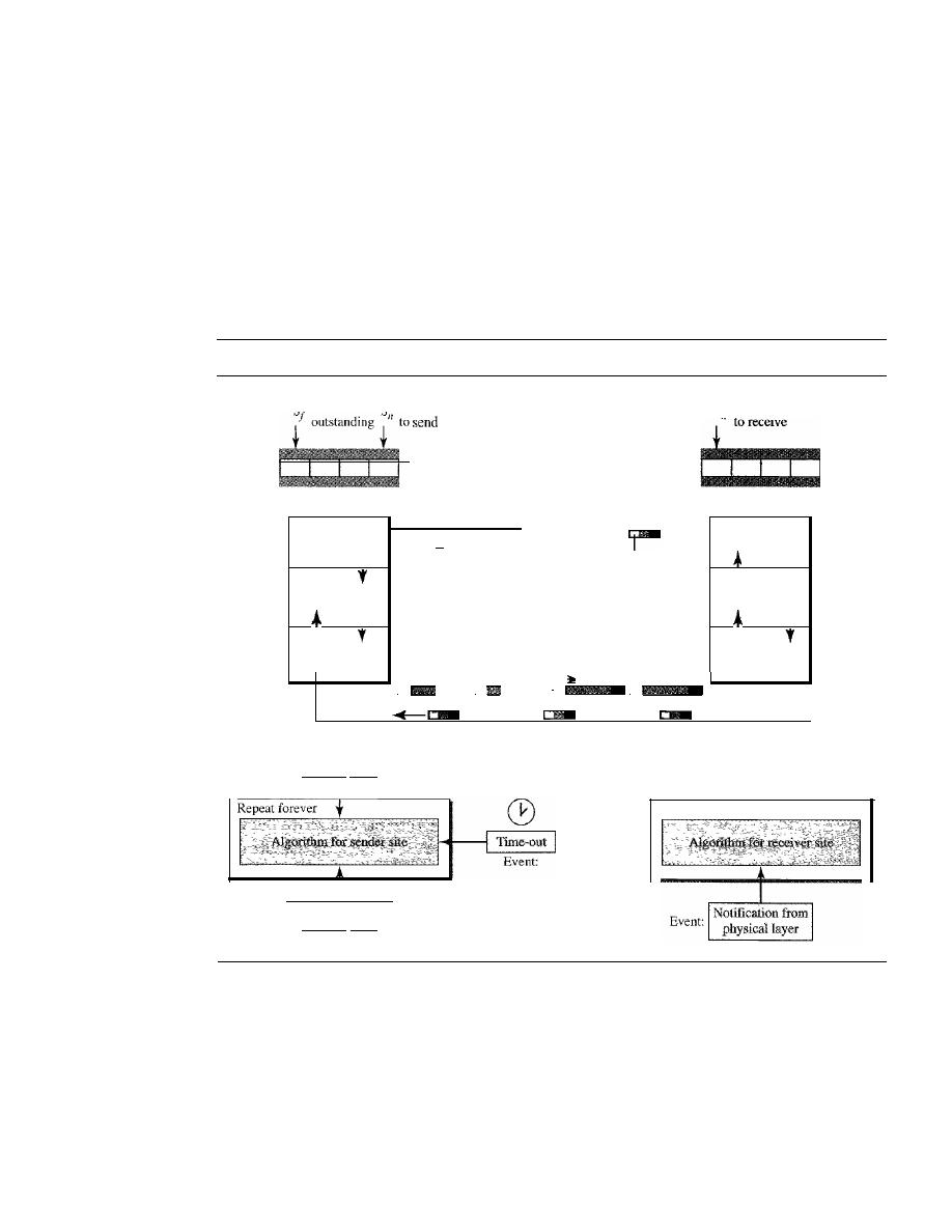
334
CHAPTER II
DATA LINK CONTROL
protocol. Those slots inside the window that are colored define frames that have arrived
out of order and are waiting for their neighbors to arrive before delivery to the network
layer.
Design
The design in this case is to some extent similar to the one we described for the
00-
Back-N, but more complicated, as shown in Figure 11.20.
Figure 11.20
Design of Selective Repeat ARQ
S First
S Next
Sender
R
Next
n
'
Receiver
Network
Data link
Physical
Data frame
ACKor NAK
Deliver
Get data
')
data
I
seqNo
ackNo
or
I
nakNo
1
I
R
I,
R
I,
ecelve Send
ecelve
Send
frame
frame
frame
frame
I
I
I
,
I
I
I
Network
Data link
Physical
Event:
I
Request from
I
network layer
I
I
E
I
Notification from
j
vent:
physical layer
Repeat forever
Window Sizes
We can now show why the size of the sender and receiver windows must be at most one-
half of
2
m
.
For an example, we choose
m
=
2, which means the size of the window is
2
m
/2,
or 2. Figure 11.21 compares a window size of 2 with a window size of 3.
If
the size of the window is 2 and all acknowledgments are lost, the timer for frame 0
expires and frame 0 is resent. However, the window of the receiver is now expecting
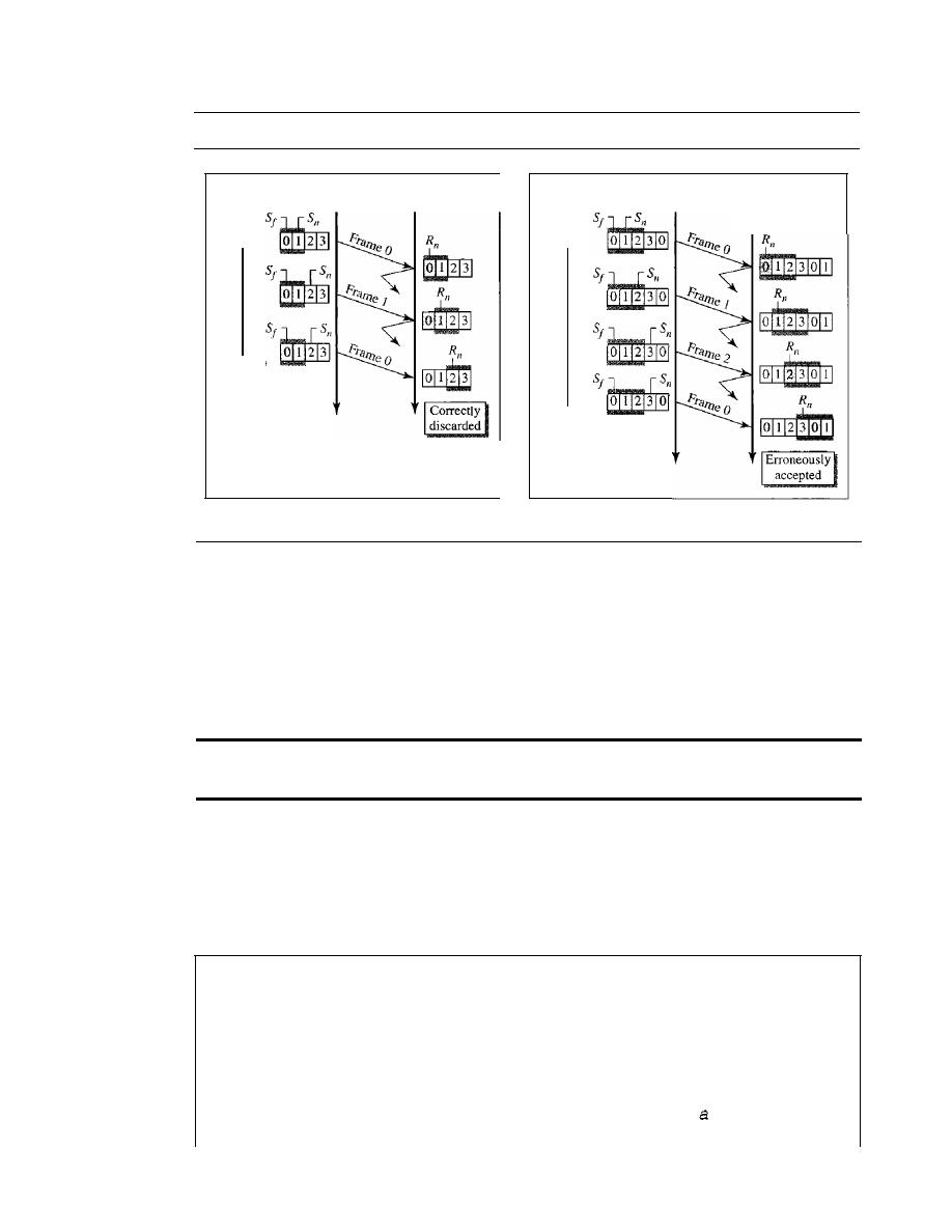
SECTION
11.5
NOISY CHANNELS
335
Figure 11.21
Selective Repeat ARQ, window size
Sender
o
1 2 3
Time-out
a. Window size
=
2
m
-
1
Receiver
Sender
Time-out
b. Window size> 2m-
1
Receiver
frame 2, not frame 0, so this duplicate frame is correctly discarded. When the size of
the window is 3 and all acknowledgments are lost, the sender sends a duplicate of
frame O. However, this time, the window of the receiver expects to receive frame 0 (0 is
part of the window), so it accepts frame 0, not as a duplicate, but as the first frame in
the next cycle. This is clearly an error.
In Selective Repeat ARQ, the size of the sender and receiver window
must be at most one-half of 2
m•
Algorithms
Algorithm 11.9 shows the procedure for the sender.
Algorithm 11.9
Sender-site Selective Repeat algorithm
WaitForEvent()i
if(Event(RequestToSend)}
{
1
=
2
m
-
1
i
2
=
Oi
3
=
Oi
4
5
hile (true)
6
{
7
8
9
//Repeat forever
//There is
packet
to sen

336
CHAPTER
11
DATA LINK CONTROL
Algorithm 11.9
Sender-site Selective Repeat algorithm (continued)
}
while{sf
<
ackNo)
{
Purge (sf);
stopTimer
(Sf) ;
Sf
=
Sf
+
1;
}
if(Event{ArrivalNotification»
IIACK arrives
{
Receive{frame);
I/Receive ACK or NAK
if{corrupted{frame»
Sleep ();
i f (FrameType
==
NAK)
if
(nakNo between Sf and So)
{
resend{nakNo);
StartTimer{nakNo);
}
if
(FrameType
==
ACK)
if (ackNo between Sf and So)
{
10
11
12
13
14
15
16
17
18
19
20
21
22
23
24
25
26
27
28
29
30
31
32
33
34
35
36
37
38
39
40
41
42
43
44
45
46
47
48
}
if{Sn-S;E
>=
Sw)
Sleep { );
GetData{) ;
MakeFrame ( Sn) ;
StoreFrame{Sn);
SendFrame (Sn) ;
Sn
=
Sn
+
1;
StartTimer{Sn);
}
}
if(Event{TimeOut{t»)
{
StartTimer{t);
SendFrame{t);
}
I/If window is full
liThe timer expires
The handling of the request event is similar to that of the previous protocol except
that one timer is started for each frame sent. The arrival event is more complicated here. An ACK
or a NAK frame may arrive. If a valid NAK frame arrives, we just resend the corresponding
frame.
If
a valid ACK arrives, we use a loop to purge the buffers, stop the corresponding timer.
and move the left wall of the window. The time-out event is simpler here; only the frame which
times out is resent.
Algorithm 11.10 shows the procedure for the receiver.
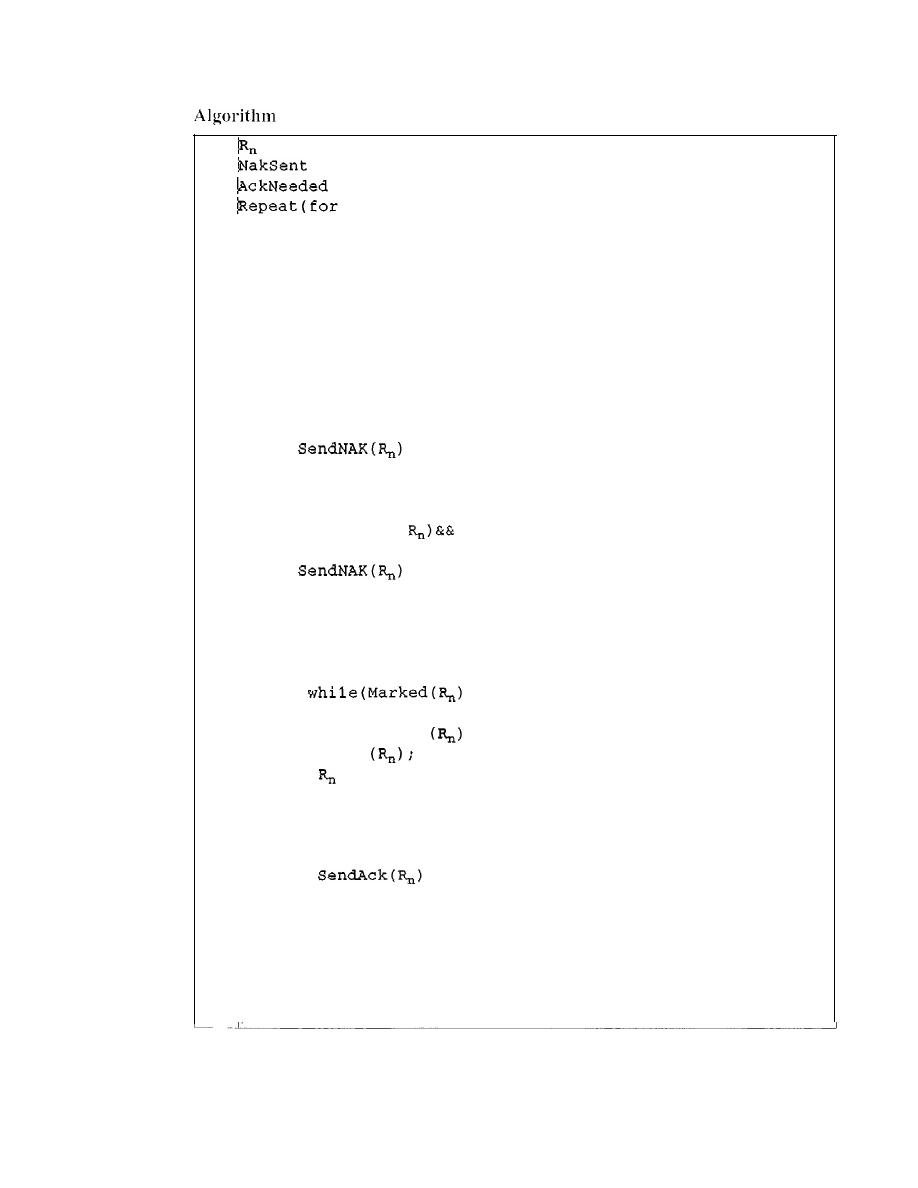
SECTION
11.5
NOISY CHANNELS
337
11.10
Receiver-site Selective Repeat algorithm
jData frame arrives
IIRepeat forever
}
if (AckNeeded) ;
{
;
AckNeeded
=
false;
NakSent
=
false;
}
}
}
Receive(Frame);
if(corrupted(Frame»&& (NOT NakSent)
{
;
NakSent
=
true;
Sleep{);
}
if(seqNo
<>
(NOT NakSent)
{
;
NakSent = true;
if {(seqNo in window)&&(IMarked(seqNo»
{
StoreFrame{seqNo)
Marked(seqNo)= true;
{
DeliverData
;
Purge
=
R
n
+
1;
AckNeeded = true;
}
WaitForEvent()i
if{Event{ArrivalNotification»
{
1
=
0;
2
= false;
3
= false;
4
all slots)
5
Marked (slot)
= false;
6
7
!while (true)
8
{
9
10
11
12
13
14
15
16
17
18
19
20
21
22
23
24
25
26
27
28
29
30
31
32
33
34
35
36
37
38
39
40
41
42
43
44
}
Analysis
Here we need more initialization. In order not to overwhelm the other side with
NAKs, we use a variable called NakSent. To know when we need to send an ACK, we use a vari-
able called AckNeeded. Both of these are initialized to false. We also use a set of variables to
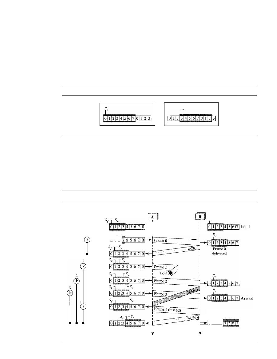
338
CHAPTER 11
DATA LINK CONTROL
mark the slots in the receive window once the corresponding frame has arrived and is stored. If
we receive a corrupted frame and a NAK has not yet been sent, we send a NAK to tell the other
site that we have not received the frame we expected.
If
the frame is not corrupted and the
sequence number is in the window, we store the frame and mark the slot. If contiguous frames,
starting from
R
n
have been marked, we deliver their data to the network layer and slide the win-
dow. Figure 11.22 shows this situation.
Figure 11.22
Delivery of data in Selective Repeat ARQ
R
ackNo sent: 3
a. Before delivery
b. After delivery
Example
11.8
This example is similar to Example 11.3 in which frame 1 is lost. We show how Selective Repeat
behaves in this case. Figure 11.23 shows the situation.
Figure 11.23
Flow diagramfor Example 11.8
Arrival
Arrival
Arrival
Receiver
R
n
I
I
I
Arrival
R
n
0
111213
4 5 6 7 Arrival
:
Frames
1,2,3
delivered
J
I
Sender
Request
Request
Request
Arrival
Initial
Sf
Sn
Request
0 1 2 3 4 5 6 7 0
o

SECTION
11.5
NOISY CHANNELS
339
One main difference is the number of timers. Here, each frame sent or resent needs a timer,
which means that the timers need to be numbered (0, 1,2, and 3). The timer for frame
°
starts
at the first request, but stops when the ACK for this frame arrives. The timer for frame I starts at
the second request, restarts when a NAK arrives, and finally stops when the last ACK arrives.
The other two timers start when the corresponding frames are sent and stop at the last arrival
event.
At the receiver site we need to distinguish between the acceptance of a frame and its
delivery to the network layer. At the second arrival, frame 2 arrives and is stored and marked
(colored slot), but it cannot be delivered because frame I is missing. At the next arrival, frame 3
arrives and is marked and stored, but still none of the frames can be delivered. Only at the last
arrival, when finally a copy of frame 1 arrives, can frames I, 2, and 3 be delivered to the net-
work layer. There are two conditions for the delivery of frames to the network layer: First, a set
of consecutive frames must have arrived. Second, the set starts from the beginning of the win-
dow. After the first alTival, there was only one frame and it started from the beginning of the
window. After the last arrival, there are three frames and the first one starts from the beginning
of the window.
Another important point is that a NAK is sent after the second arrival, but not after the third,
although both situations look the same. The reason is that the protocol does not want to crowd the
network with unnecessary NAKs and unnecessary resent frames. The second NAK would still be
NAKI to inform the sender to resend frame 1 again; this has already been done. The first NAK
sent is remembered (using the nakSent variable) and is not sent again until the frame slides. A
NAK is sent once for each window position and defines the first slot in the window.
The next point is about the ACKs. Notice that only two ACKs are sent here. The first one
acknowledges only the first frame; the second one acknowledges three frames. In Selective
Repeat, ACKs are sent when data are delivered to the network layer.
If
the data belonging to
n
frames are delivered in one shot, only one ACK is sent for all of them.
Piggybacking
The three protocols we discussed in this section are all unidirectional: data frames flow
in only one direction although control information such as ACK and NAK frames can
travel in the other direction. In real life, data frames are normally flowing in both direc-
tions: from node A to node B and from node B to node A. This means that the control
information also needs to flow in both directions. A technique called piggybacking is
used to improve the efficiency of the bidirectional protocols. When a frame is carrying
data from A to B, it can also carry control information about arrived (or lost) frames
from B; when a frame is carrying data from B to A, it can also carry control information
about the arrived (or lost) frames from A.
We show the design for a Go-Back-N ARQ using piggybacking in Figure 11.24.
Note that each node now has two windows: one send window and one receive window.
Both also need to use a timer. Both are involved in three types of events: request, arrival,
and time-out. However, the arrival event here is complicated; when a frame arrives, the
site needs to handle control information as well as the frame itself. Both of these concerns
must be taken care of in one event, the arrival event. The request event uses only the send
window at each site; the arrival event needs
to
use both windows.
An important point about piggybacking is that both sites must use the same algo-
rithm. This algorithm is complicated because it needs to combine two arrival events
into one. We leave this task as an exercise.
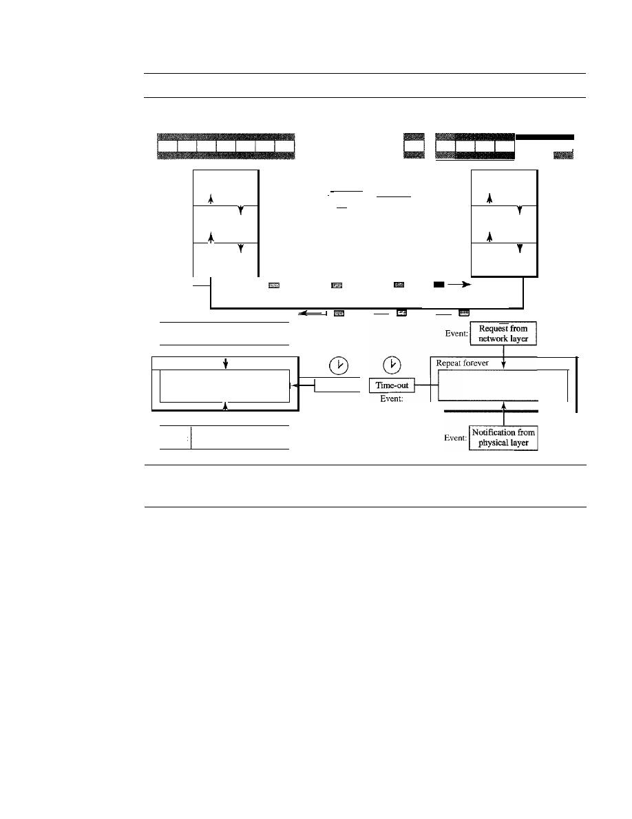
340
CHAPTER
11
DATA LINK CONTROL
Figure 11.24
Design ofpiggybacking in Go-Back-N ARQ
Send
window
Receive
window
Receive
Send
window
window
Network
Data link
Physical
ackNo
Deliver
Get
I
-Frame
Deliver
Get
I
I
'f
I
I
seqNo
I
I
I
R
I,
R
I,
ecelve Send
ecelve Send
frame
frame
frame
frame
I
,
. l
_ I
I
_ I
-,
-
Network
Data link
Physical
Event:
I
Request from
I
'
network layer
I
Repeat forever
Algorithm for
Time-out
I
sending and receiving
Event:
I
E
Notification from I
vent:
physical layer
Algorithm for
sending and receiving
11.6
HDLC
High-level Data Link Control (HDLC)
is a bit-oriented protocol for communication
over point-to-point and multipoint links.
It
implements the ARQ mechanisms we dis-
cussed in this chapter.
Configurations and Transfer Modes
HDLC provides two common transfer modes that can be used in different configura-
tions:
normal response mode (NRM)
and
asynchronous balanced mode (ABM).
Normal Response Mode
In normal response mode (NRM), the station configuration is unbalanced. We have one
primary station and multiple secondary stations.
A primary station
can send commands;
a
secondary station
can only respond. The
NRM
is used
for
both point-to-point and
multiple-point links, as shown in Figure 11.25.
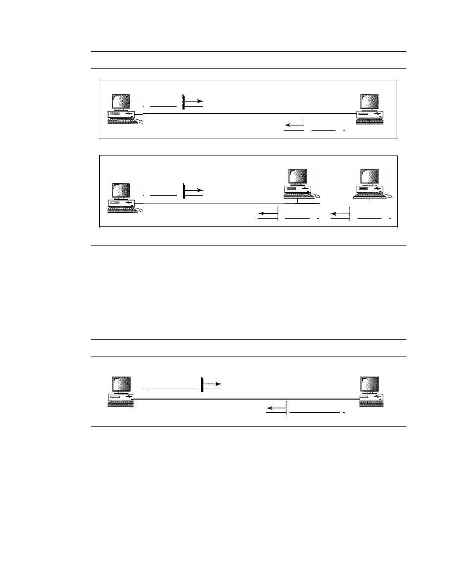
SECTION 11.6
HDLC
341
Figure 11.25
Normal response mode
Primary
I
Command
a. Point-to-point
Secondary
Response
I
Secondary
Secondary
Primary
I
Command
b. Multipoint
Response
I
Response
I
Asynchronous Balanced Mode
In asynchronous balanced mode (ABM), the configuration is balanced. The link is
point-to-point, and each station can function as a primary and a secondary (acting as
peers), as shown in Figure 11.26. This is the common mode today.
Figure 11.26
Asynchronous balanced mode
Combined
Combined
I
Command/response
Command/response
I
Frames
To provide the flexibility necessary to support all the options possible in the modes and
configurations just described, HDLC defines three types of frames: information frames
(I-frames), supervisory frames (S-frames), and unnumbered frames (V-frames). Each
type of frame serves as an envelope for the transmission of a different type of message.
I-frames are used to transport user data and control information relating to user data
(piggybacking). S-frames are used only to transport control information. V-frames are
reserved for system management. Information carried by V-frames is intended for manag-
ing the link itself.
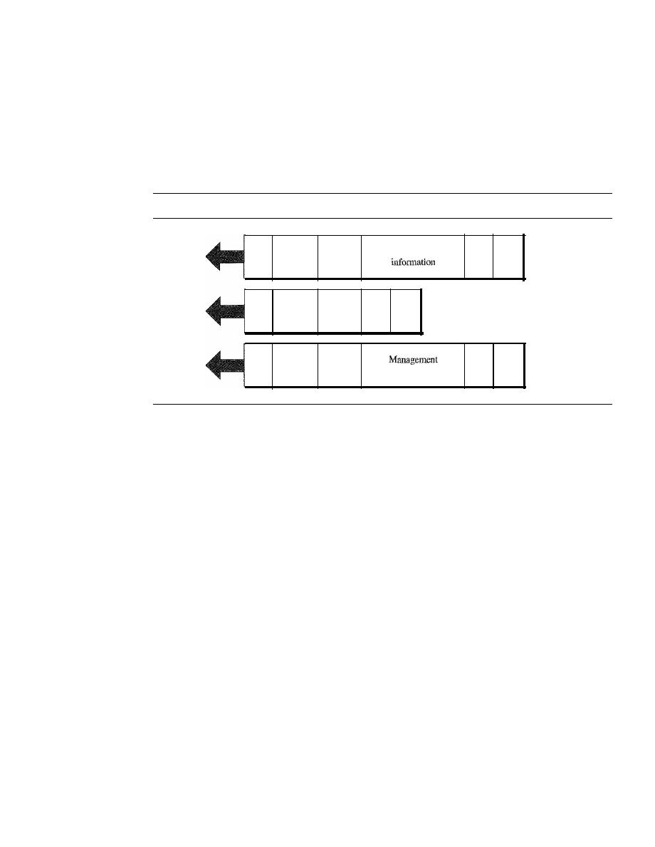
342
CHAPTER
11
DATA LINK CONTROL
Frame Format
Each frame in HDLC may contain up to six fields, as shown in Figure 11.27: a begin-
ning flag field, an address field, a control field, an information field, a frame check
sequence (FCS) field, and an ending flag field. In multiple-frame transmissions, the
ending flag of one frame can serve as the beginning flag of the next frame.
Figure 11.27
HDLC frames
Flag
Address
Control
FCS
Flag
S-frame
Flag
Address
Control
Flag
Address
Control
User
infonnatlon
PCS
Flag
I-frame
FCS
Flag
U-frame
Fields
Let us now discuss the fields and their use in different frame types.
o
Flag field. The flag field of an HDLC frame is an 8-bit sequence with the bit pattern
01111110 that identifies both the beginning and the end of a frame and serves as a
synchronization pattern for the receiver.
o
Address field. The second field of an HDLC frame contains the address of the
secondary station. If a primary station created the frame, it contains a
to
address. If
a secondary creates the frame, it contains afrom address. An address field can be
1 byte or several bytes long, depending on the needs of the network. One byte can
identify up to 128 stations
(l
bit is used for another purpose). Larger networks
require multiple-byte address fields. If the address field is only 1 byte, the last bit
is always a 1. If the address is more than 1 byte, all bytes but the last one will end
with 0; only the last will end with 1. Ending each intermediate byte with 0 indi-
cates to the receiver that there are more address bytes to come.
o
Control field. The control field is a 1- or 2-byte segment of the frame used for
flow and error control. The interpretation of bits in this field depends on the frame
type. We discuss this field later and describe its format for each frame type.
o
Information field. The information field contains the user's data from the net-
work layer or management information. Its length can vary from one network to
another.
o
FCS field. The frame check sequence (FCS) is the HDLC error detection field.
It
can contain either a 2- or 4-byte ITU-T CRC.
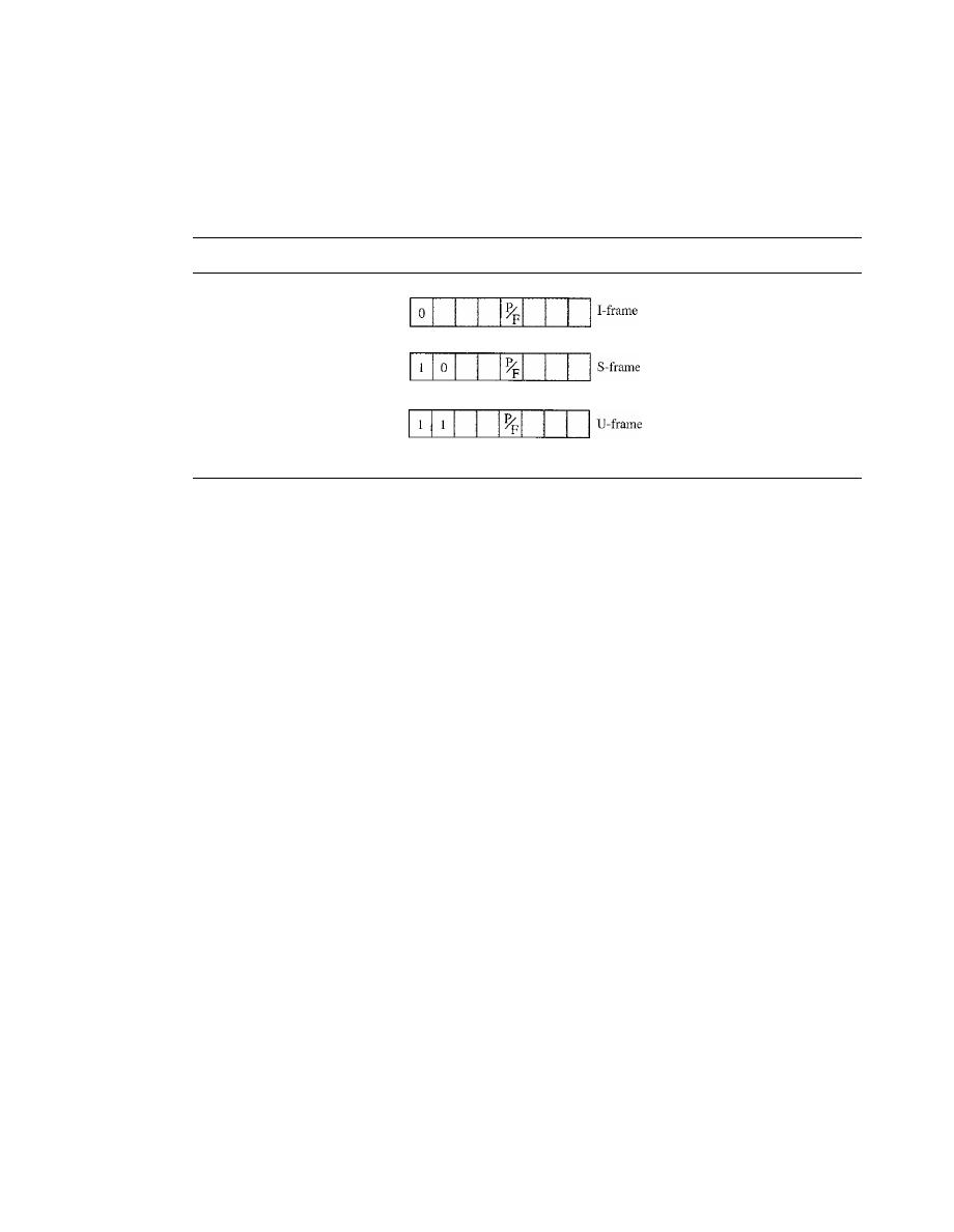
SECTION
11.6
HDLC
343
Control Field
The control field determines the type of frame and defines its functionality. So let us
discuss the format of this field in greater detail. The format is specific for the type of
frame, as shown in Figure 11.28.
Figure 11.28
Control field format for the different frame types
N(S)
N(R)
Code
N(R)
Code
Code
Control Field for I-Frames
I-frames are designed to carry user data from the network layer. In addition, they can
include flow and error control information (piggybacking). The subfields in the control
field are used to define these functions. The first bit defines the type. If the first bit of
the control field is 0, this means the frame is an I-frame. The next 3 bits, called
N(S),
define the sequence number of the frame. Note that with 3 bits, we can define a
sequence number between
°
and 7; but in the extension format, in which the control
field is 2 bytes, this field is larger. The last 3 bits, called
N(R),
correspond to the
acknowledgment number when piggybacking is used. The single bit between
N(S)
and
N(R)
is called the
PIF
bit. The
PIP
field is a single bit with a dual purpose.
It
has mean-
ing only when it is set (bit
=
1) and can mean poll or final.
It
means
poll
when the frame
is sent by a primary station to a secondary (when the address field contains the address
of the receiver).
It
means
final
when the frame is sent by a secondary to a primary
(when the address field contains the address of the sender).
Control Fieldfor S-Frames
Supervisory frames are used for flow and error control whenever piggybacking is either
impossible or inappropriate (e.g., when the station either has no data of its own to send or
needs to send a command or response other than an acknowledgment). S-frames do not
have information fields.
If
the first 2 bits of the control field is 10, this means the frame
is an S-frame. The last 3 bits, called
N(R),
corresponds to the acknowledgment number
(ACK) or negative acknowledgment number (NAK) depending on the type of S-frame.
The 2 bits called code is used to define the type of S-frame itself. With 2 bits, we can
have four types of S-frames, as described below:
o
Receive ready (RR).
If
the value of the code subfield is 00, it is an RR S-frame.
This kind of frame acknowledges the receipt of a safe and sound frame or
group of frames. In this case, the value
N(R)
field defines the acknowledgment
number.

344
CHAPTER
11
DATA LINK CONTROL
o
Receive not ready (RNR).
If
the value of the code subfield is 10, it is an RNR
S-frame. This kind of frame is an RR frame with additional functions.
It
acknowledges the receipt of a frame or group of frames, and it announces that
the receiver is busy and cannot receive more frames.
It
acts as a kind of conges-
tion control mechanism by asking the sender to slow down. The value of
NCR)
is the acknowledgment number.
o
Reject (REJ).
If
the value of the code subfield is 01, it is a REJ S-frame. This is a
NAK frame, but not like the one used for Selective Repeat ARQ.
It
is a NAK that
can be used in
Go-Back-N
ARQ to improve the efficiency of the process by
informing the sender, before the sender time expires, that the last frame is lost or
damaged. The value of
NCR)
is the negative acknowledgment number.
o
Selective reject (SREJ). If the value of the code subfield is 11, it is an SREJ S-frame.
This is a NAK frame used in Selective Repeat ARQ. Note that the HDLC Protocol
uses the term
selective reject
instead of
selective repeat.
The value of
N(R)
is the neg-
ative acknowledgment number.
Control Fieldfor V-Frames
Unnumbered frames are used to exchange session management and control infonnation
between connected devices. Unlike S-frames, U-frames contain an information field,
but one used for system management information, not user data. As with S-frames,
however, much of the infonnation carried by U-frames is contained in codes included
in the control field. U-frame codes are divided into two sections: a 2-bit prefix before
the PtF bit and a 3-bit suffix after the PtF bit. Together, these two segments (5 bits) can
be used to create up to 32 different types of U-frames. Some of the more common types
are shown in Table 11.1.
Table 11.1
control command and response
Code
Command
Response
Meaning
00 001
SNRM
Set normal response mode
11 011
SNRME
Set normal response mode, extended
11 100
SABM
DM
Set asynchronous balanced mode or disconnect mode
11110
SABME
Set asynchronous balanced mode, extended
00 000
UI
UI
Unnumbered information
00 110
UA
Unnumbered acknowledgment
00 010
DISC
RD
Disconnect or request disconnect
10 000
SIM
RIM
Set initialization mode or request information mode
00 100
UP
Unnumbered poll
11 001
RSET
Reset
11 101
XID
XID
Exchange ID
10 001
FRMR
FRMR
Frame reject
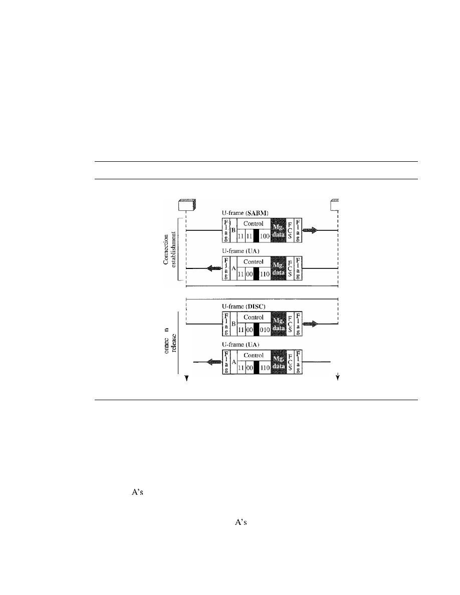
SECTION
11.6
HDLC
345
Example
11.9:
Connection/Disconnection
Figure 11.29 shows how V-frames can be used for connection establishment and connection
release. Node A asks for a connection with a set asynchronous balanced mode (SABM) frame;
node B gives a positive response with an unnumbered acknowledgment (VA) frame. After these
two exchanges, data can be transferred between the two nodes (not shown in the figure). After
data transfer, node A sends a DISC (disconnect) frame to release the connection; it is confirmed
by node B responding with a VA (unnumbered acknowledgment).
Figure
11.29
Example of connection and disconnection
Node A
NodeB
Data transfer
o
. -
-
u
Time
I
I
Time
Example 11.10: Piggybacking without Error
Figure 11.30 shows an exchange using piggybacking. Node A begins the exchange of
information with an I-frame numbered 0 followed by another I-frame numbered 1. Node B
piggybacks its acknowledgment of both frames onto an I-frame of its own. Node B's first
I-frame is also numbered 0
[N(S)
field] and contains a 2 in its
N(R)
field, acknowledging the
receipt of
frames 1 and 0 and indicating that it expects frame 2 to arrive next. Node B
transmits its second and third I-frames (numbered 1 and 2) before accepting further
frames from node A. Its
N(R)
information, therefore, has not changed: B frames 1 and 2
indicate that node B is still expecting
frame 2 to arrive next. Node A has sent all its
data. Therefore, it cannot piggyback an acknowledgment onto an I-frame and sends an S-frame
instead. The RR code indicates that A is still ready to receive. The number 3 in the
N(R)
field
tells B that frames 0,
1,
and 2 have all been accepted and that A is now expecting frame
number 3.
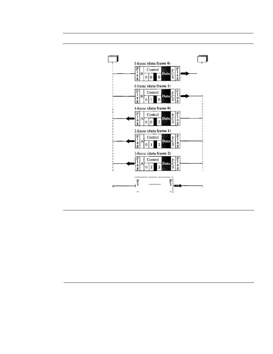
346
CHAPTER
11
DATA LINK CONTROL
Figure 11.30
Example ofpiggybacking without error
Node A
NodeB
S-frame (RR), an ACK 3
Control
F
B
C
a
\ORR
3S
a
g
g
y
Time
y
Time
Example
11.11:
Piggybacking with Error
Figure 11.31 shows an exchange in which a frame is lost. Node B sends three data frames (0, 1,
and 2), but frame 1 is lost. When node A receives frame 2, it discards it and sends a
REI
frame for
frame 1. Note that the protocol being used is Go-Back-N with the special use of an REI frame as
a NAK frame. The NAK frame does two things here: It confirms the receipt of frame
°
and
declares that frame 1 and any following frames must be resent. Node B, after receiving the REI
frame, resends frames 1 and 2. Node A acknowledges the receipt by sending an RR frame (ACK)
with acknowledgment number 3.
11.7
POINT-TO-POINT PROTOCOL
Although HDLC is a general protocol that can be used for both point-to-point and multi-
point configurations, one of the most common protocols for point-to-point access is the
Point-to-Point Protocol (PPP).
Today, millions of Internet users who need to connect
their home computers to the server of an Internet service provider use PPP. The majority
of these users have a traditional modem; they are connected to the Internet through a
telephone line, which provides the services of the physical layer. But to control and
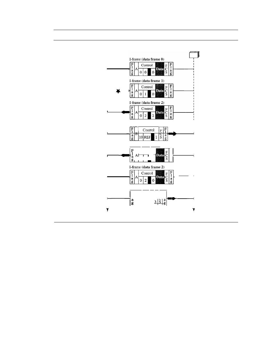
SECTION
11.7
POINT-TO-POINT PROTOCOL
347
Figure 11.31
Example ofpiggybacking with error
Node A
NodeB
Lost
Discarded
S-frame (REJ 1), a NAK
F
B
C
IOREJ
I-frame (data frame
1)
Control
__
0 1
0
FI
Resent
a
g
Resent
1
1
I
I
Time
S-frame (RR 3), an ACK
F
Control
F F
I B
C I
toRR
Time
manage the transfer of data, there is a need for a point-to-point protocol at the data link
layer. PPP is by far the most common.
PPP provides several services:
1. PPP defines the format of the frame to be exchanged between devices.
2. PPP defines how two devices can negotiate the establishment of the link and the
exchange of data.
3. PPP defines how network layer data are encapsulated in the data link frame.
4. PPP defines how two devices can authenticate each other.
5.
PPP provides multiple network layer services supporting a variety of network layer
protocols.
6. PPP provides connections over multiple links.
7. PPP provides network address configuration. This is particularly useful when a home
user needs a temporary network address to connect to the Internet.
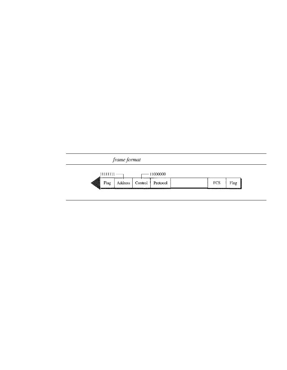
348
CHAPTER
11
DATA LINK CONTROL
On the other hand, to keep PPP simple, several services are missing:
I.
PPP does not provide flow control. A sender can send several frames one after
another with no concern about overwhelming the receiver.
2. PPP has a very simple mechanism for error control. A CRC field is used to detect
errors.
If
the frame is corrupted, it is silently discarded; the upper-layer protocol
needs to take care of the problem. Lack of error control and sequence numbering
may cause a packet to be received out of order.
3. PPP does not provide a sophisticated addressing mechanism to handle frames in a
multipoint configuration.
Framing
PPP is a byte-oriented protocol. Framing is done according to the discussion of byte-
oriented protocols at the beginning of this chapter.
Frame Format
Figure 11.32 shows the format of a PPP frame. The description of each field follows:
Figure 11.32
PPP
1 byte
1 byte
1 byte
1 or 2 bytes
Payload
Variable
2 or 4 bytes
1 byte
o
Flag. A PPP frame starts and ends with a I-byte flag with the bit pattern 01111110.
Although this pattern is the same as that used in HDLC, there is a big difference.
PPP is a byte-oriented protocol; HDLC is a bit-oriented protocol. The flag is treated
as a byte, as we will explain later.
o
Address. The address field in this protocol is a constant value and set to 11111111
(broadcast address). During negotiation (discussed later), the two parties may agree
to omit this byte.
o
Control. This field is set to the constant value 11000000 (imitating unnumbered
frames in HDLC). As we will discuss later, PPP does not provide any flow control.
Error control is also limited to error detection. This means that this field is not needed
at all, and again, the two parties can agree, during negotiation, to omit this byte.
o
Protocol. The protocol field defines what is being carried in the data field: either
user data or other information. We discuss this field in detail shortly. This field is
by default 2 bytes long, but the two parties can agree to use only I byte.
o
Payload field. This field carries either the user data or other information that we will
discuss shortly. The data field is a sequence of bytes with the default of a maximum
of 1500 bytes; but this can be changed during negotiation. The data field is byte-
stuffed if the flag byte pattern appears in this field. Because there is no field defining
the size of the data field, padding is needed if the size is less than the maximum
default value or the maximum negotiated value.
o
FCS. The frame check sequence (FCS) is simply a 2-byte or 4-byte standard CRe.
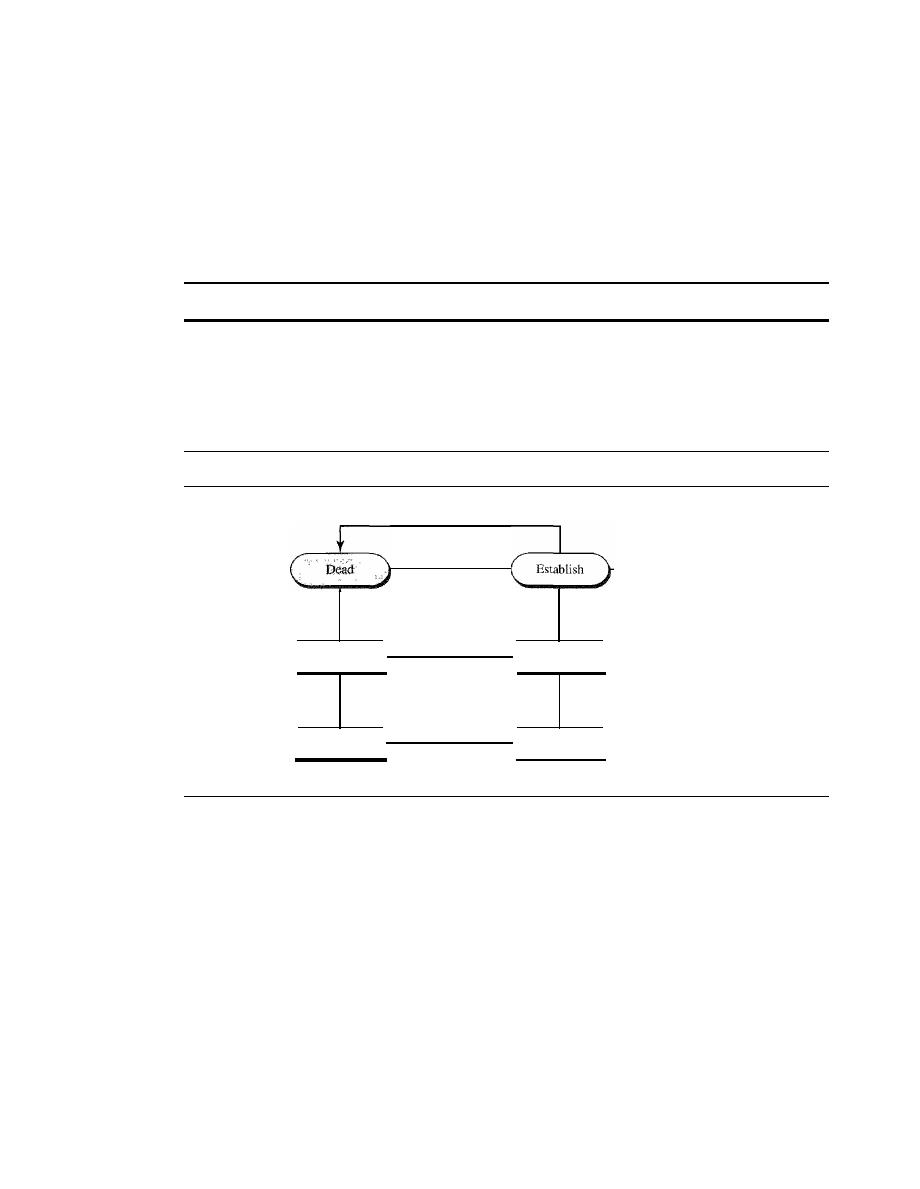
SECTION
11.7
POINT-TO-POINT PROTOCOL
349
Byte Stuffing
The similarity between PPP and
HDLe
ends at the frame format. PPP, as we discussed
before, is a byte-oriented protocol totally different from
HDLC.
As a byte-oriented
protocol, the flag in PPP is a byte and needs to be escaped whenever
it
appears in the
data section of the frame. The escape byte is 01111101, which means that every time
the flaglike pattern appears in the data, this extra byte is stuffed to tell the receiver that
the next byte is not a flag.
PPP
is a byte-oriented protocol using byte stuffing with the escape byte 01111101.
Transition
Phases
A PPP connection goes through phases which can be shown in a
transition phase
diagram (see Figure 11.33).
Figure 11.33
Transition phases
Failed
Carrier
dropped
Tenmnate
Done
Carrier
detected
Failed
Options agreed
by both sides
Authenticate
Authentication
successful
If authentication
not needed
Network layer
configuration
Network
D
Dead. In the dead phase the link is not being used. There is no active carrier (at
the physical layer) and the line is quiet.
D
Establish. When one of the nodes starts the communication, the connection goes into
this phase. In this phase, options are negotiated between the two parties.
If
the negoti-
ation is successful, the system goes to the authentication phase (if authentication is
required) or directly to the networking phase. The link control protocol packets, dis-
cussed shortly, are used for this purpose. Several packets may be exchanged here.
D
Authenticate. The authentication phase is optional; the two nodes may decide,
during the establishment phase, not to skip this phase. However, if they decide to
proceed with authentication, they send several authentication packets, discussed
later. If the result is successful, the connection goes to the networking phase; other-
wise, it goes to the termination phase.
D
Network. In the network phase, negotiation for the network layer protocols takes
place. PPP specifies that two nodes establish a network layer agreement before data at
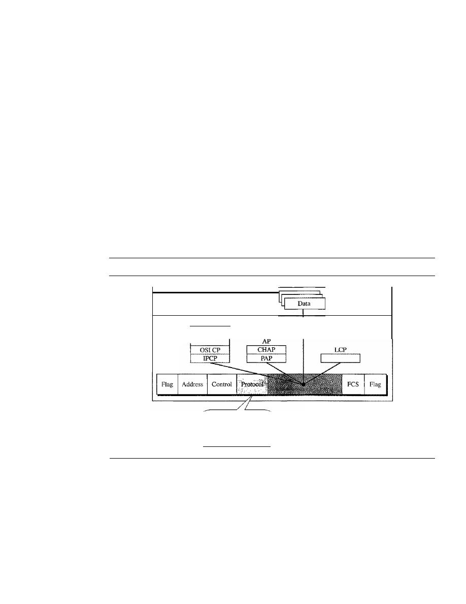
350
CHAPTER
11
DATA LINK CONTROL
the network layer can be exchanged. The reason is that PPP supports multiple proto-
cols at the network layer. If a node is running multiple protocols simultaneously at the
network layer, the receiving node needs to know which protocol will receive the data.
o
Open.
In the open phase, data transfer takes place. When a connection reaches
this phase, the exchange of data packets can be started. The connection remains in
this phase until one of the endpoints wants to terminate the connection.
o
Terminate.
In the termination phase the connection is terminated. Several packets
are exchanged between the two ends for house cleaning and closing the link.
Multiplexing
Although PPP is a data link layer protocol, PPP uses another set of other protocols to
establish the link, authenticate the parties involved, and carry the network layer data. Three
sets of protocols are defined to make PPP powetful: the Link Control Protocol (LCP), two
Authentication Protocols (APs), and several Network Control Protocols (NCPs). At any
moment, a PPP packet can carry data from one of these protocols in its data field, as shown
in Figure 11.34. Note that there is one LCP, two APs, and several NCPs. Data may also
come from several different network layers.
Figure
11.34
Multiplexing in PPP
Network
layer
Data link
layer
Data from different
networking protocols
NCP
•
•
•
LCP: OxC021
AP: OxC023 and OxC223
NCP: Ox8021 and
.
Data: Ox0021 and
.
LCP: Link Control Protocol
AP: Authentication Protocol
NCP: Network Control Protocol
Link Control Protocol
The Link Control Protocol (LCP) is responsible for establishing, maintaining, config-
uring, and terminating links.
It
also provides negotiation mechanisms to set options
between the two endpoints. Both endpoints of the link must reach an agreement about
the options before the link can be established. See Figure 11.35.
All LCP packets are carried in the payload field of the PPP frame with the protocol
field set to C02 1 in hexadecimal.
The code field defines the type of LCP packet. There are 11 types of packets as
shown in Table 11.2.
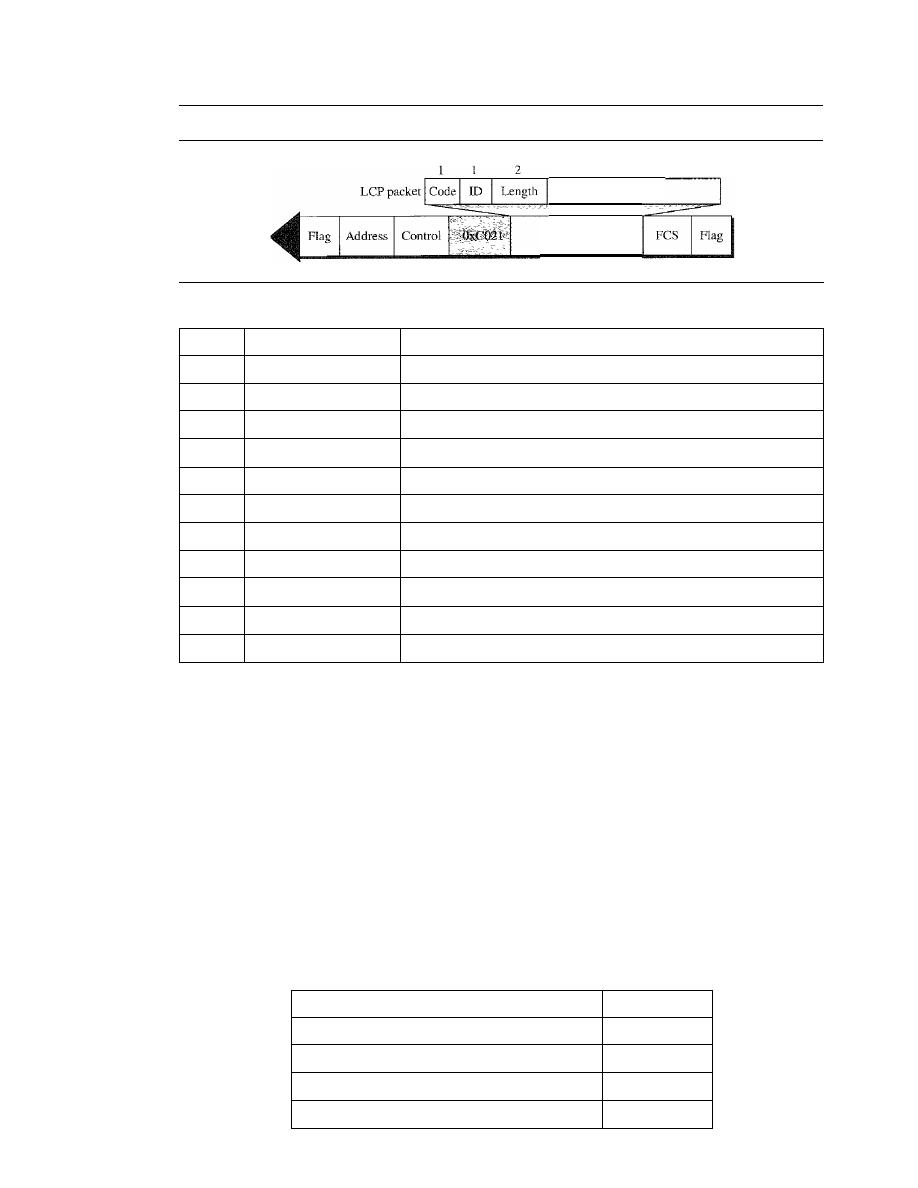
SECTION
11.7
POINT-TO-POINT PROTOCOL
351
Figure 11.35
LCP packet encapsulated in aframe
Variable
Infonnation
Payload
(and padding)
Table 11.2
LCP packets
Code
Packet Type
Description
OxOl
Coofigure-request
Contains the list of proposed options and their values
Ox02
Configure-ack
Accepts all options proposed
Ox03
Configure-nak
Announces that some options are oot acceptable
Ox04
Configure-reject
Announces that some options are not recognized
Ox05
Terminate-request
Request to shut down the line
Ox06
Terminate-ack
Accept the shutdown request
Ox07
Code-reject
Announces an unknown code
Ox08
Protocol-reject
Announces an unknown protocol
Ox09
Echo-request
A
type of hello message to check if the other end is alive
OxOA
Echo-reply
The response to the echo-request message
OxOB
Discard-request
A request to discard the packet
There are three categories of packets. The first category, comprising the first four
packet types, is used for link configuration during the establish phase. The second cate-
gory, comprising packet types 5 and 6, is used for link tennination during the termina-
tion phase. The last five packets are used for link monitoring and debugging.
The ID field holds a value that matches a request with a reply. One endpoint inserts
a value in this field, which will be copied into the reply packet. The length field defines
the length of the entire LCP packet. The information field contains information, such as
options, needed for some LCP packets.
There are many options that can be negotiated between the two endpoints. Options
are inserted in the information field of the configuration packets. In this case, the infor-
mation field is divided into three fields: option type, option length, and option data. We
list some of the most common options in Table 11.3.
Table 11.3
Common options
Option
Default
Maximum receive unit (payload field size)
1500
Authentication protocol
None
Protocol field compression
Off
Address and control field compression
Off
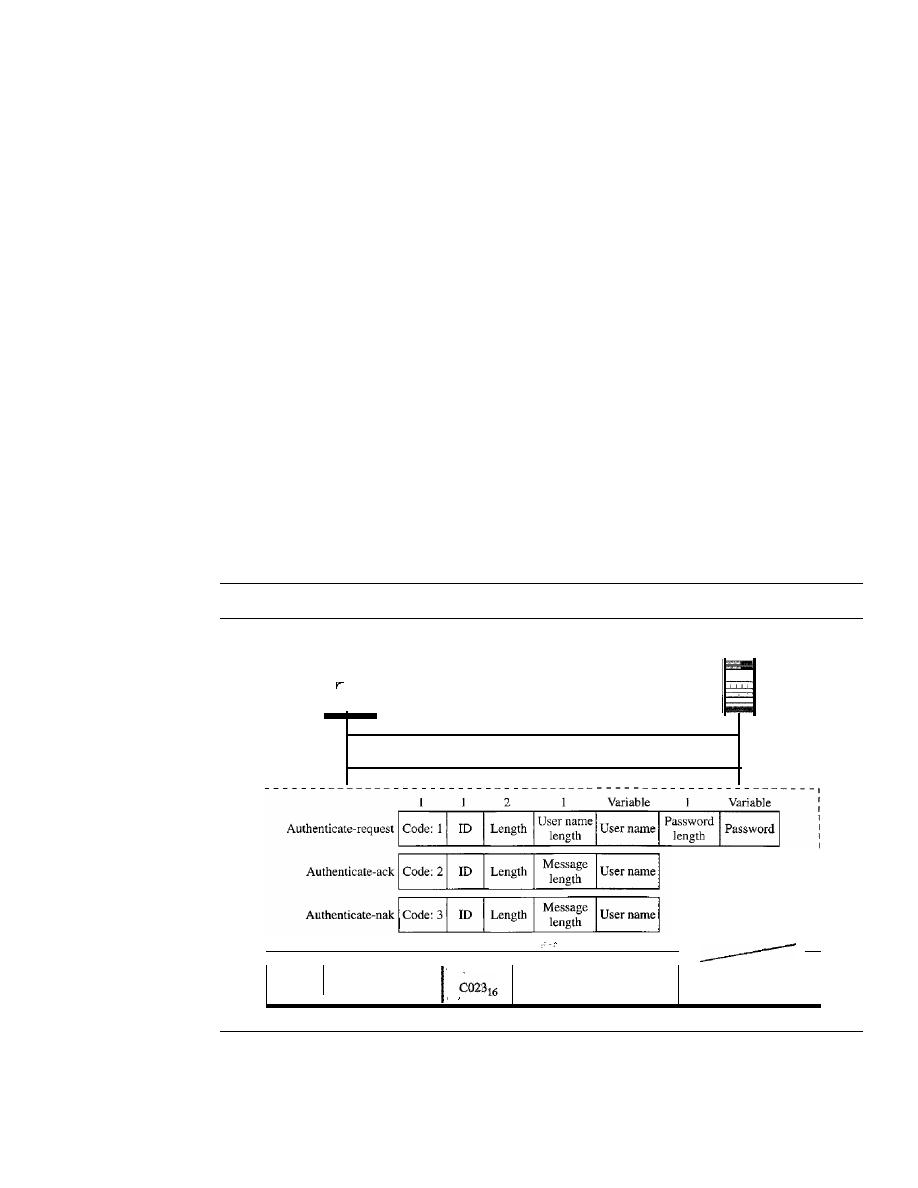
352
CHAPTER
11
DATA LINK CONTROL
Authentication Protocols
Authentication plays a very important role in PPP because PPP is designed for use over
dial-up links where verification of user identity is necessary.
Authentication means vali-
dating the identity of a user who needs to access a set of resources. PPP has created two
protocols for authentication: Password Authentication Protocol and Challenge Handshake
Authentication Protocol. Note that these protocols are used during the authentication phase.
PAP
The
Password Authentication Protocol (PAP) is a simple authentication pro-
cedure with a two-step process:
1. The user who wants to access a system sends an authentication identification
(usually the user name) and a password.
2. The system checks the validity of the identification and password and either accepts
or denies connection.
Figure 11.36 shows the three types of packets used by PAP and how they are actually
exchanged. When a PPP frame is carrying any PAP packets, the value of the protocol
field is OxC023. The three PAP packets are authenticate-request, authenticate-ack, and
authenticate-nak. The first packet is used by the user to send the user name and pass-
word. The second is used by the system to allow access. The third is used by the system
to deny access.
Figure 11.36
PAP packets encapsulated in a PPP frame
System
User
Authenticate-request
Authenticate-ack or authenticate-nak
PAP packets
I
Flag
Address
I
Control
Payload
FeS
I
Flag
I
I
(and padding)
CHAP
The
Challenge Handshake Authentication Protocol (CHAP) is a three-way
hand-shaking authentication protocol that provides greater security than PAP.
In this
method, the password is kept secret; it is never sent online.
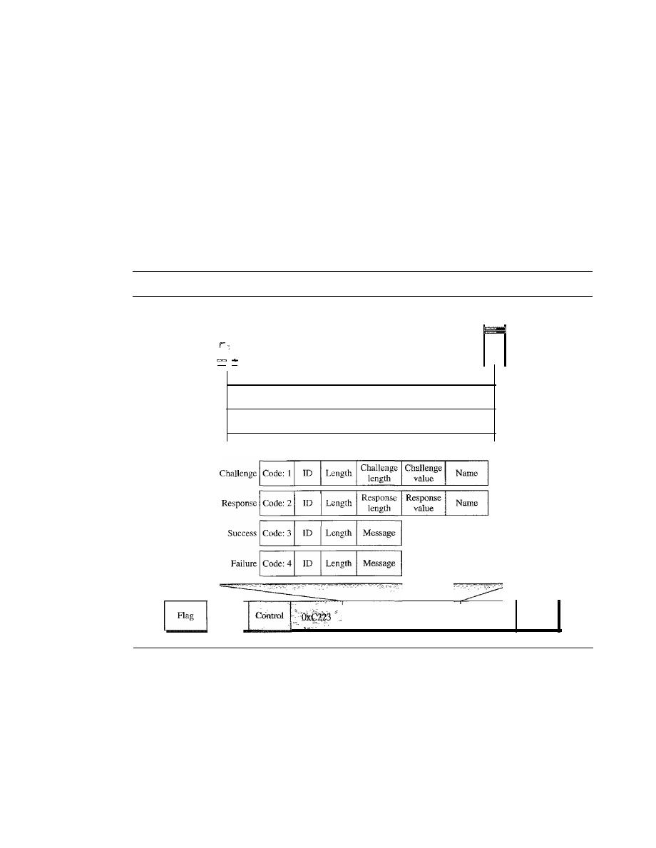
SECTION
11.7
POINT-TO-POINT PROTOCOL
353
1. The system sends the user a challenge packet containing a challenge value, usually
a few bytes.
2. The user applies a predefined function that takes the challenge value and the user's
own password and creates a result. The user sends the result in the response packet
to the system.
3. The system does the same.
It
applies the same function to the password of the user
(known to the system) and the challenge value to create a result. If the result created is
the same as the result sent in the response packet, access is granted; otherwise, it is
denied. CHAP is more secure than PAP, especially if the system continuously changes
the challenge value. Even if the intruder learns the challenge value and the result, the
password is still secret. Figure 11.37 shows the packets and how they are used.
Figure 11.37
CHAP packets encapsulated in a PPP frame
User
Challenge
Response
Success or failure
System
2
Variable
Variable
Address
-
Payload
(and padding)
CHAP packets
FCS
Flag
CHAP packets are encapsulated in the PPP frame with the protocol value C223 in
hexadecimal. There are four CHAP packets: challenge, response, success, and failure.
The first packet is used by the system to send the challenge value. The second is used by
the user to return the result of the calculation. The third is used by the system to allow
access to the system. The fourth is used by the system to deny access to the system.
Network Control Protocols
PPP is a multiple-network layer protocol. It can carry a network layer data packet from
protocols defined by the Internet, OSI, Xerox, DECnet, AppleTalk, Novel, and so on.
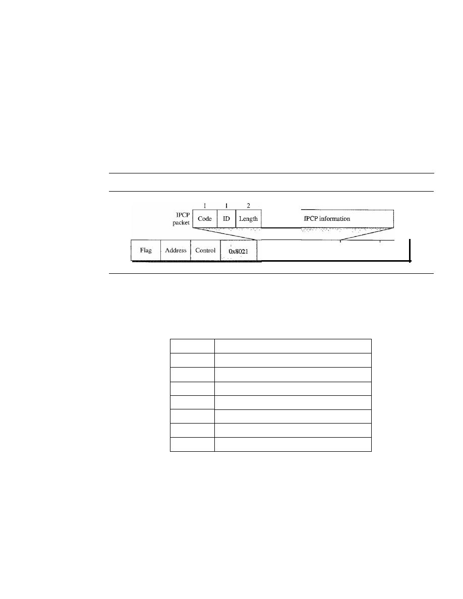
354
CHAPTER 11
DATA LINK CONTROL
To do this, PPP has defined a specific Network Control Protocol for each network pro-
tocol. For example, IPCP (Internet Protocol Control Protocol) configures the link for
carrying IP data packets. Xerox CP does the same for the Xerox protocol data packets,
and so on. Note that none of the NCP packets carry network layer data; they just
configure the link at the network layer for the incoming data.
IPCP
One NCP protocol is the Internet Protocol Control Protocol (IPCP). This
protocol configures the link used to carry IP packets in the Internet. IPCP is especially
of interest to us. The format of an IPCP packet is shown in Figure 11.38. Note that the
value of the protocol field in hexadecimal is 8021.
Figure 11.38
fPCP packet encapsulated in PPP frame
Variable
Payload
(and padding)
FCS
Flag
IPCP defines seven packets, distinguished by their code values, as shown in
Table
11.4.
Table 11.4
Code value for IPCP packets
Code
IPCP Packet
OxO!
Configure-request
Ox02
Configure-ack
Ox03
Configure-nak
Ox04
Configure-reject
Ox05
Terminate-request
Ox06
Terminate-ack
Ox07
Code-reject
Other Protocols
There are other NCP protocols for other network layer protocols.
The OSI Network Layer Control Protocol has a protocol field value of 8023; the Xerox
NS IDP Control Protocol has a protocol field value of 8025; and so on. The value of the
code and the format of the packets for these other protocols are the same as shown in
Table
11.4.
Data/rom the Network Layer
After the network layer configuration is completed by one of the NCP protocols, the
users can exchange data packets from the network layer. Here again, there are different
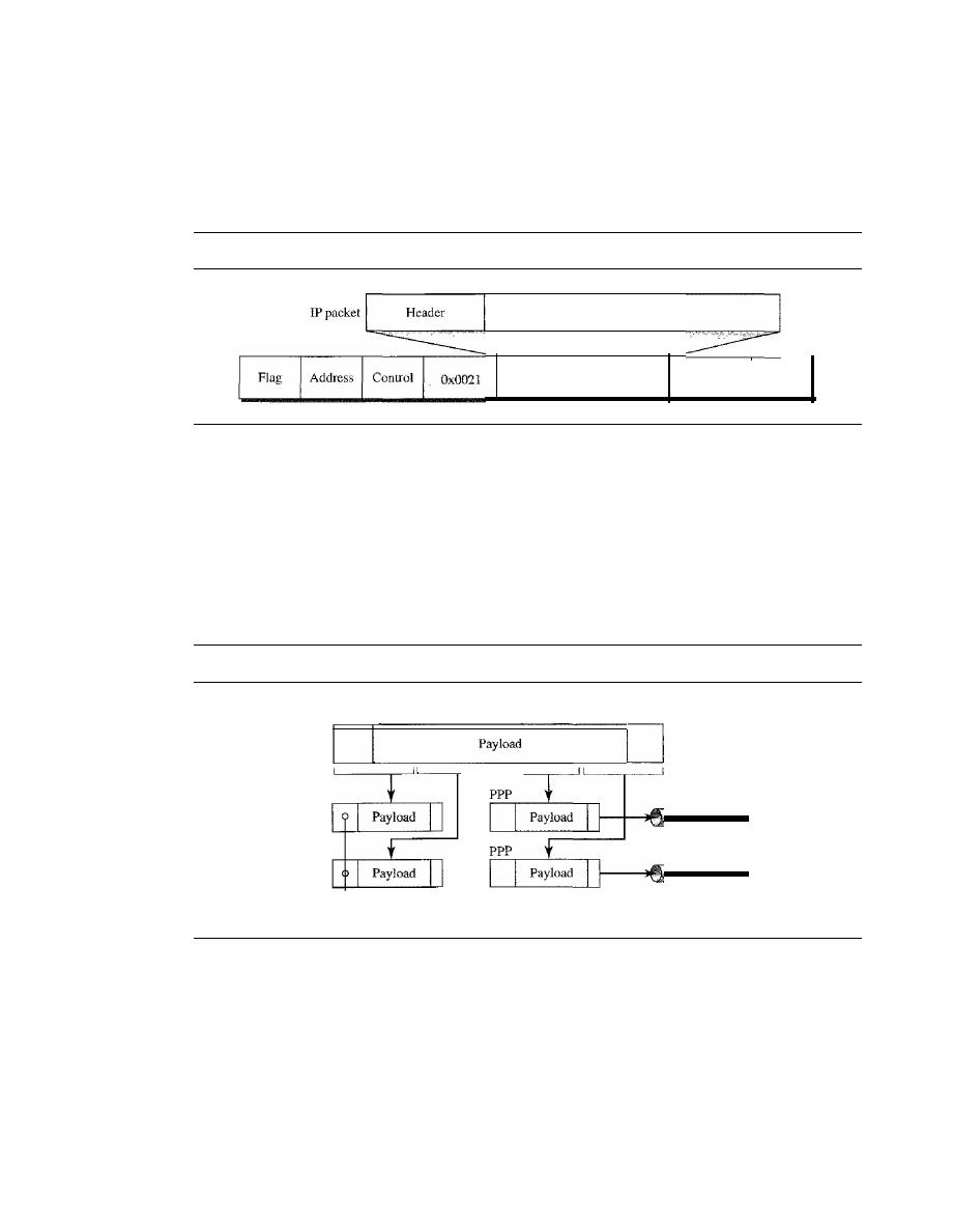
SECTION 11.7
POINT-TO-POINT PROTOCOL
355
protocol fields for different network layers. For example, if PPP is carrying data from
the IP network layer, the field value is 0021 (note that the three rightmost digits are the
same as for IPCP).
If
PPP is carrying data from the OSI network layer, the value of the
protocol field is 0023, and so on. Figure 11.39 shows the frame for IP.
Figure 11.39
IP datagram encapsulated in a PPP frame
User data
Payload
(and padding)
FCS
Flag
Multilink PPP
PPP was originally designed for a single-channel point-to-point physical link. The avail-
ability of multiple channels in a single point-to-point link motivated the development of
Multilink PPP. In this case, a logical PPP frame is divided into several actual PPP
frames. A segment of the logical frame is carried in the payload of an actual PPP frame,
as shown in Figure 11.40. To show that the actual PPP frame is carrying a fragment of a
Figure 11.40
Multilink PPP
Channel 2
Channell
PPP
Logical PPP
Payload
PPP
Protocol filed: Ox003d
logical PPP frame, the protocol field is set to Ox003d. This new development adds com-
plexity. For example, a sequence number needs to be added to the actual PPP frame to
show a fragment's position in the logical frame.
Example 11.12
Let us go through the phases followed by a network layer packet as it is transmitted through a
PPP connection. Figure 11.41 shows the steps. For simplicity, we assume unidirectional move-
ment of data from the user site to the system site (such as sending an e-mail through an ISP).
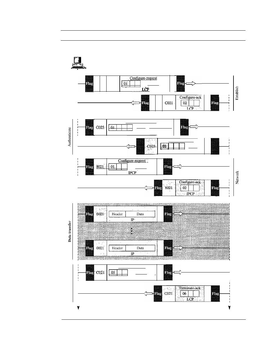
356
CHAPTER
11
DATA LINK CONTROL
Figure 11.41
An example
User
System
i
Options
Authenticate-ack
Name
PAP
Authenticate-request
Name
O-P-a-ss-w-o-rd-I
PAP
Options
Terminate-request
Options
LCP
[
Time
Time

SECTION 11.9
KEY TERMS
357
The first two frames show link establishment. We have chosen two options (not shown in the
figure): using PAP for authentication and suppressing the address control fields. Frames 3 and 4
are for authentication. Frames 5 and 6 establish the network layer connection using IPCP.
The next several frames show that some IP packets are encapsulated in the PPP frame. The
system (receiver) may have been running several network layer protocols, but it knows that the
incoming data must be delivered to the IP protocol because the NCP protocol used before the data
transfer was IPCP.
After data transfer, the user then terminates the data link connection, which is acknowledged
by the system. Of COUrse the user or the system could have chosen to terminate the network layer
IPCP and keep the data link layer running if it wanted to run another NCP protocol.
The example is trivial, but it points out the similarities of the packets in LCP, AP, and
NCP.
It
also shows the protocol field values and code numbers for particular protocols.
11.8
RECOMMENDED READING
For more details about subjects discussed in this chapter, we recommend the following
books. The items in brackets [...] refer to the reference list at the end of the text.
Books
A discussion of data link control can be found in [GW04], Chapter 3 of [Tan03], Chapter 7
of [Sta04], Chapter 12 of [Kes97], and Chapter 2 of [PD03]. More advanced materials can
be found in [KMK04].
11.9
KEY TERMS
acknowledgment (ACK)
asynchronous balanced mode (ABM)
automatic repeat request (ARQ)
bandwidth-delay product
bit-oriented protocol
bit stuffing
byte stuffing
Challenge Handshake Authentication
Protocol (CHAP)
character-oriented protocol
data link control
error control
escape character (ESC)
event
fixed-size framing
flag
flow control
framing
Go-Back-N ARQ Protocol
High-level Data Link Control (HDLC)
information frame (I-frame)
Internet Protocol Control Protocol (IPCP)
Link Control Protocol (LCP)
negative acknowledgment (NAK)
noiseless channel
noisy channel
normal response mode (NRM)
Password Authentication Protocol (PAP)
piggybacking
pipelining
Point-to-Point Protocol (PPP)
primary station

358
CHAPTER
11
DATA LINK CONTROL
receive sliding window
secondary station
Selective Repeat ARQ
Protocol
send sliding window
sequence number
Simplest Protocol
sliding window
Stop-and-Wait ARQ Protocol
Stop-and-Wait Protocol
supervisory frame (S-frame)
transition phase
unnumbered frame (D-frame)
variable-size framing
11.10
SUMMARY
o
Data link control deals with the design and procedures for communication between
two adjacent nodes: node-to-node communication.
o
Framing in the data link layer separates a message from one source to a destination,
or from other messages going from other sources to other destinations,
o
Frames can be of fixed or variable size. In fixed-size framing, there is no need for
defining the boundaries of frames; in variable-size framing, we need a delimiter
(flag) to define the boundary of two frames.
o
Variable-size framing uses two categories of protocols: byte-oriented (or character-
oriented) and bit-oriented. In a byte-oriented protocol, the data section of a frame
is a sequence of bytes; in a bit-oriented protocol, the data section of a frame is a
sequence of bits.
o
In byte-oriented (or character-oriented) protocols, we use byte stuffing; a special
byte added to the data section of the frame when there is a character with the same
pattern as the flag.
o
In bit-oriented protocols, we use bit stuffing; an extra 0 is added to the data section
of the frame when there is a sequence of bits with the same pattern as the flag.
o
Flow control refers to a set of procedures used to restrict the amount of data that the
sender can send before waiting for acknowledgment. Error control refers to methods
of error detection and correction.
o
For the noiseless channel, we discussed two protocols: the Simplest Protocol and
the Stop-and-Wait Protocol. The first protocol has neither flow nor error control;
the second has no error control. In the Simplest Protocol, the sender sends its
frames one after another with no regards to the receiver. In the Stop-and-Wait Pro-
tocol, the sender sends one frame, stops until it receives confirmation from the
receiver, and then sends the next frame.
D
For the noisy channel, we discussed three protocols: Stop-and-Wait ARQ,
00-
Back-N,
and Selective Repeat ARQ. The Stop-and-Wait ARQ Protocol, adds a
simple error control mechanism to the Stop-and-Wait Protocol. In the Oo-Back-N
ARQ Protocol, we can send several frames before receiving acknowledgments,
improving the efficiency of transmission. In the Selective Repeat ARQ protocol we
avoid unnecessary transmission by sending only frames that are corrupted.
D
Both Oo-Back-N and Selective-Repeat Protocols use a sliding window. In
00-
Back-N
ARQ, if m is the number of bits for the sequence number, then the size of

SECTION
11.11
PRACTICE SET
359
the send window must be less than 2
m
;
the size of the receiver window is always 1.
In Selective Repeat ARQ, the size of the sender and receiver window must be at
most one-half of
2
m
.
o
A technique called piggybacking is used to improve the efficiency of the bidirec-
tional protocols. When a frame is carrying data from A to B, it can also carry control
information about frames from B; when a frame is carrying data from B to A, it can
also carry control information about frames from A.
o
High-level Data Link Control (HDLC) is a bit-oriented protocol for communication
over point-to-point and multipoint links. However, the most common protocols for
point-to-point access is the Point-to-Point Protocol (PPP), which is a byte-oriented
protocol.
11.11
PRACTICE SET
Review Questions
1.
Briefly describe the services provided by the data link layer.
2. Define framing and the reason for its need.
3. Compare and contrast byte-oriented and bit-oriented protocols. Which category
has been popular in the past (explain the reason)? Which category is popular now
(explain the reason)?
4. Compare and contrast byte-stuffing and bit-stuffing. Which technique is used in
byte-oriented protocols? Which technique is used in bit-oriented protocols?
5. Compare and contrast flow control and error control.
6. What are the two protocols we discussed for noiseless channels in this chapter?
7. What are the three protocols we discussed for noisy channels in this chapter?
8. Explain the reason for moving from the Stop-and-Wait ARQ Protocol to the
00-
Back-N ARQ Protocol.
9. Compare and contrast the Go-Back-N ARQ Protocol with Selective-RepeatARQ.
10. Compare and contrast HDLC with PPP. Which one is byte-oriented; which one is
bit-oriented?
11. Define piggybacking and its usefulness.
12. Which of the protocols described in this chapter utilize pipelining?
Exercises
13.
Byte-stuff the data in Figure 11.42.
Figure 11.42
Exercise 13
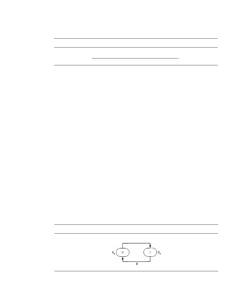
360
CHAPTER
11
DATA LINK CONTROL
14. Bit-stuff the data in Figure 11.43.
Figure 11.43
Exercise 14
1000111111100111110100011111111111000011111
I
15. Design two simple algorithms for byte-stuffing. The first adds bytes at the sender;
the second removes bytes at the receiver.
16. Design two simple algorithms for bit-stuffing. The first adds bits at the sender; the
second removes bits at the receiver.
17. A sender sends a series of packets to the same destination using 5-bit sequence
numbers. If the sequence number starts with 0, what is the sequence number after
sending 100 packets?
18. Using 5-bit sequence numbers, what is the maximum size of the send and receive
windows for each of the following protocols?
a. Stop-and-Wait ARQ
b. Go-Back-N ARQ
c. Selective-Repeat ARQ
19. Design a bidirectional algorithm for the Simplest Protocol using piggybacking.
Note that the both parties need to use the same algorithm.
20. Design a bidirectional algOIithm for the Stop-and-Wait Protocol using piggybacking.
Note that both parties need to use the same algorithm.
21. Design a bidirectional algorithm for the Stop-and-Wait ARQ Protocol using piggy-
backing. Note that both parties need to use the same algorithm.
22. Design a bidirectional algorithm for the Go-Back-N ARQ Protocol using piggy-
backing. Note that both parties need to use the same algorithm.
23. Design a bidirectional algorithm for the Selective-Repeat ARQ Protocol using piggy-
backing. Note that both parties need to use the same algorithm.
24. Figure 11.44 shows a state diagram to simulate the behavior of Stop-and-Wait ARQ
at the sender site.
Figure 11.44
Exercise 24
A
The states have a value of
Sn
(0 or
1).
The arrows shows the transitions. Explain the
events that cause the two transitions labeled A and B.
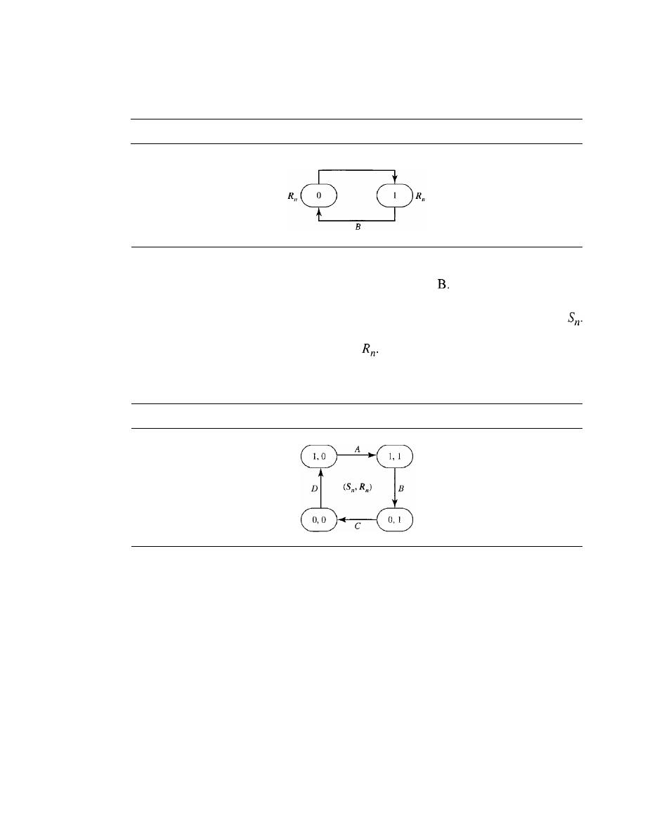
SECTION
11.11
PRACTICE SET
361
25. Figure 11.45 shows a state diagram to simulate the behavior of Stop-and-Wait
ARQ at the receiver site.
Figure 11.45
Exercise 25
A
The states have a value of R
n
(0 or
1).
The arrows shows the transitions. Explain
the events that cause the two transitions labeled A and
26. In Stop-and-Wait ARQ, we can combine the state diagrams of the sender and
receiver in Exercises 24 and 25. One state defines the combined values of
R
n
and
This means that we can have four states, each defined by
(x, y),
where
x
defines the
value of
Sn
and y defines the value of
In other words, we can have the four
states shown in Figure 11.46. Explain the events that cause the four transitions
labeled A, B, C, and D.
Figure 11.46
Exercise 26
27. The timer of a system using the Stop-and-Wait ARQ Protocol has a time-out of 6 ms.
Draw the flow diagram similar to Figure 11.11 for four frames if the round trip delay
is 4 ms. Assume no data frame or control frame is lost or damaged.
28. Repeat Exercise 27 if the time-out is 4 ms and the round trip delay is 6.
29. Repeat Exercise 27 if the first frame (frame 0) is lost.
30. A system uses the Stop-and-Wait ARQ Protocol. If each packet carries 1000 bits of
data, how long does it take to send 1 million bits of data if the distance between the
sender and receiver is 5000
KIn
and the propagation speed is 2 x 10
8
m? Ignore trans-
mission, waiting, and processing delays. We assume no data or control frame is lost
or damaged.
31.
Repeat Exercise 30 using the Go-back-N ARQ Protocol with a window size of 7.
Ignore the overhead due to the header and trailer.
32. Repeat Exercise 30 using the Selective-Repeat ARQ Protocol with a window
size of 4. Ignore the overhead due to the header and the trailer.

CHAPTER 12
Multiple
Access
In Chapter 11 we discussed data link control, a mechanism which provides a link with
reliable communication. In the protocols we described, we assumed that there is an
available dedicated link (or channel) between the sender and the receiver. This assump-
tion mayor may not be true.
If,
indeed, we have a dedicated link, as when we connect
to the Internet using PPP as the data link control protocol, then the assumption is true
and we do not need anything else.
On the other hand, if we use our cellular phone to connect to another cellular phone,
the channel (the band allocated to the vendor company) is not dedicated. A person a few
feet away from us may be using the same channel to talk to her friend.
We can consider the data link layer as two sublayers. The upper sublayer is responsi-
ble for data link control, and the lower sublayer is responsible for resolving access to the
shared media. If the channel is dedicated, we do not need the lower sublayer. Figure 12.1
shows these two sublayers in the data link layer.
Figure 12.1
Data link layer divided into two functionality-oriented sublayers
Data link layer
Data link control
Multiple-access resolution
We will see in Chapter 13 that the IEEE has actually made this division for LANs.
The upper sublayer that is responsible for flow and error control is called the logical
link control (LLC) layer; the lower sublayer that is mostly responsible for multiple-
access resolution is called the media access control (MAC) layer.
When nodes or stations are connected and use a common link, called a multipoint
or broadcast link, we need a multiple-access protocol to coordinate access to the link.
The problem of controlling the access to the medium is similar to the rules of speaking
363
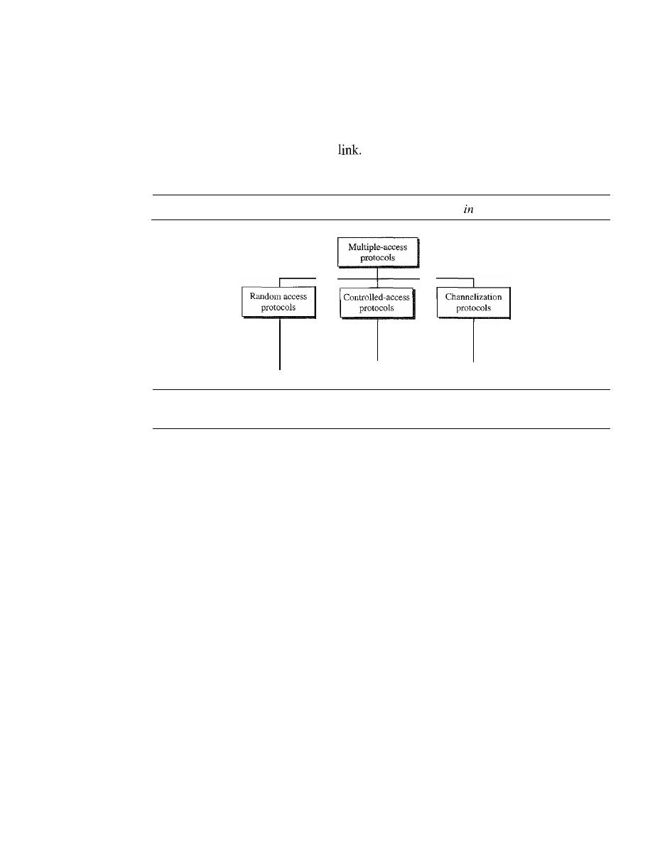
364
CHAPTER
12
MULTIPLE ACCESS
in an assembly. The procedures guarantee that the right to speak is upheld and ensure
that two people do not speak at the same time, do not interrupt each other, do not
monopolize the discussion, and so on.
The situation is similar for multipoint networks. Many formal protocols have been
devised to handle access to a shared
We categorize them into three groups. Protocols
belonging to each group are shown in Figure 12.2.
Figure 12.2
Taxonomy of multiple-access protocols discussed
this chapter
12.1
ALOHA
CSMA
CSMA/CD
CSMA/CA
RANDOM ACCESS
Reservation
Polling
Token passing
FDMA
TDMA
CDMA
In random access or contention methods, no station is superior to another station and
none is assigned the control over another. No station permits, or does not permit,
another station to send. At each instance, a station that has data to send uses a procedure
defined by the protocol to make a decision on whether or not to send. This decision
depends on the state of the medium (idle or busy). In other words, each station can
transmit when it desires on the condition that it follows the predefined procedure,
including the testing of the state of the medium.
Two features give this method its name. First, there is no scheduled time for a station
to transmit. Transmission is random among the stations. That is why these methods are
called
random access.
Second, no rules specify which station should send next. Stations
compete with one another to access the medium. That is why these methods are also
called
contention
methods.
In a random access method, each station has the right to the medium without being
controlled by any other station. However, if more than one station tries to send, there is
an access conflict-collision-and the frames will be either destroyed or modified. To
avoid access conflict or to resolve it when it happens, each station follows a procedure
that answers the following questions:
o
When can the station access the medium?
o
What can the station do if the medium is busy?
o
How can the station determine the success or failure of the transmission?
o
What can the station do if there is an access conflict?
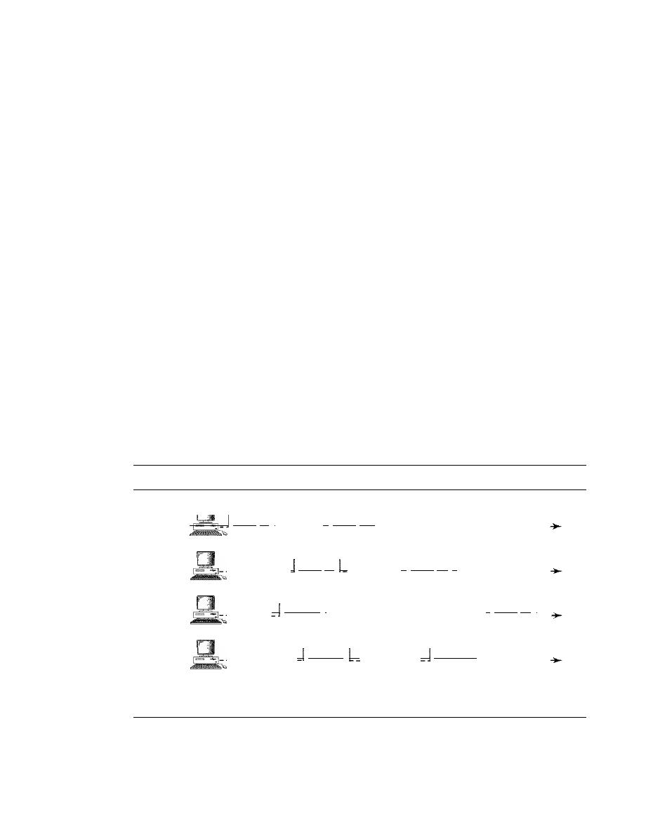
SECTION
12.1
RANDOM ACCESS
365
The random access methods we study in this chapter have evolved from a very
interesting protocol known as ALOHA, which used a very simple procedure called
multiple access (MA). The method was improved with the addition of a procedure that
forces the station to sense the medium before transmitting. This was called carrier sense
multiple access. This method later evolved into two parallel methods: carrier sense
multiple access with collision detection (CSMAlCD) and carrier sense multiple access
with collision avoidance
(CSMA/CA). CSMA/CD
tells the station what to do when a
collision is detected.
CSMA/CA
tries to avoid the collision.
ALOHA
ALOHA, the earliest random access method, was developed at the University of Hawaii
in early 1970.
It
was designed for a radio (wireless) LAN, but it can be used on any
shared medium.
It
is obvious that there are potential collisions in this arrangement. The medium is
shared between the stations. When a station sends data, another station may attempt to
do so at the same time. The data from the two stations collide and become garbled.
Pure ALOHA
The original ALOHA protocol is called pure ALOHA. This is a simple, but elegant
protocol. The idea is that each station sends a frame whenever it has a frame to send.
However, since there is only one channel to share, there is the possibility of collision
between frames from different stations. Figure 12.3 shows an example of frame collisions
in pure ALOHA.
Figure 12.3
Frames in a pure ALOHA network
[J
Station 1
Frame 1.1
1
J
Frame
1.21
Time
Station 2
Frame 2.1
-'
Frame 2.2
L
Time
Station 3
Frame3.1
1
J
Frame 3.2
I__
Time
Station 4
Frame4.1
Frame4.21
Time
Collision
duration
Collision
duration
There are four stations (unrealistic assumption) that contend with one another for
access to the shared channel. The figure shows that each station sends two frames; there
are a total of eight frames on the shared medium. Some of these frames collide because
multiple frames are in contention for the shared channel. Figure 12.3 shows that only
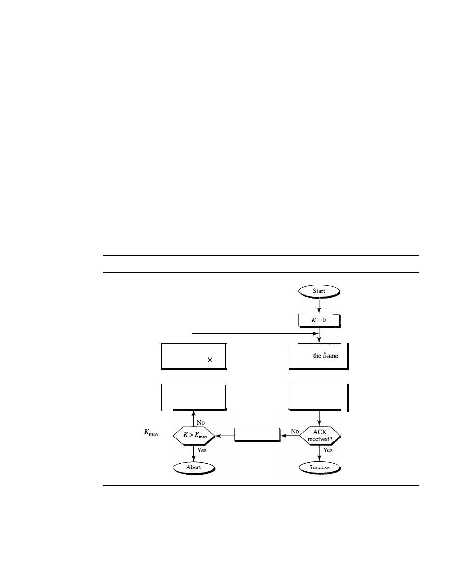
366
CHAPTER 12
MULTIPLE ACCESS
two frames survive: frame 1.1 from station 1 and frame 3.2 from station 3. We need to
mention that even if one bit of a frame coexists on the channel with one bit from
another frame, there is a collision and both will be destroyed.
It
is obvious that we need to resend the frames that have been destroyed during
transmission. The pure ALOHA protocol relies on acknowledgments from the receiver.
When a station sends a frame, it expects the receiver to send an acknowledgment.
If
the
acknowledgment does not arrive after a time-out period, the station assumes that the
frame (or the acknowledgment) has been destroyed and resends the frame.
A collision involves two or more stations.
If
all these stations try to resend their
frames after the time-out, the frames will collide again. Pure ALOHA dictates that
when the time-out period passes, each station waits a random amount of time before
resending its frame. The randomness will help avoid more collisions. We call this time
the back-off time
T
B.
Pure ALOHA has a second method to prevent congesting the channel with retrans-
mitted frames. After a maximum number of retransmission attempts
K
max'
a station
must give up and
try
later. Figure 12.4 shows the procedure for pure ALOHA based on
the above strategy.
Figure 12.4
Procedure for pure
ALOHA protocol
K:
Number of attempts
T
p :
Maximum propagation time
T
fr :
Average transmission time for a frame
T
B :
Back-off time
WaitTBtime
(Ta=Rx Tpor R
T
fr )
Choose a random
number R between
o
and
2
K
-1
Station has
a frame to send
Send
Wait time-Qut time
(2
X
T
p)
is
normally 15
K=K+
1
The time-out period is equal to the maximum possible round-trip propagation delay,
which is twice the amount of time required to send a frame between the two most widely
separated stations (2 x T
p )'
The back-off time T
B
is a random value that normally depends
on
K
(the number of attempted unsuccessful transmissions). The formula for
T
B
depends on
the implementation. One common formula is the binary exponential back-off. In this
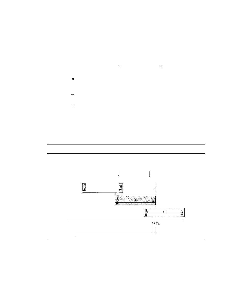
SECTION
12.1
RANDOM ACCESS
367
method, for each retransmission, a multiplier in the range 0 to
2
K
-
1 is randomly chosen
and multiplied by
T
p
(maximum propagation time) or
T
rr
(the average time required to
send out a frame) to find
T
B'
Note that in this procedure, the range of the random numbers
increases after each collision. The value of
K
max
is usually chosen as 15.
Example
12.1
The stations on a wireless
ALOHA
network are a maximum of
600
km
apart.
If
we assume that
signals propagate at
3
x 10
8
mis, we find
T
p
(600
x 10
5
) /
(3
x 10
8
)
2
ms. Now we can find the
value of
T
B
for different values of
K.
a. For
K
1, the range is
{O,
I}. The station needs to generate a random number with a
value of
0
or
1.
This means that
T
B
is either
°
ms
(0
x
2)
or
2
ms
(l
x
2),
based on the
outcome of the random variable.
b. For
K
2,
the range is
{O,
1,
2,
3}. This means that
T
B
can be 0,
2,
4, or 6 ms, based on
the outcome of the random variable.
c. For
K
3, the range is
to,
1,2,3,4,5,6,
7}. This means that
T
B
can be
0,2,4, ... , 14
ms,
based on the outcome of the random variable.
d. We need to mention that if
K
>
10,
it is normally set to 10.
Vulnerable time
Let us find the length of time, the
vulnerable time, in which there
is a possibility of collision. We assume that the stations send fixed-length frames with
each frame taking
T
fr
S
to send. Figure 12.5 shows the vulnerable time for station A.
Figure 12.5
Vulnerable time for pure ALOHA protocol
B's end
collides with
A's beginning
A's end
collides with
C's beginning
,
,
,
B
-
,
::1
C
I·
Vulnerable time
=
2
X
T
fr
Time
Station A sends a frame at time
t. Now imagine station B has already sent a frame
between
t -
T
fr
and
t.
This leads to a collision between the frames from station A and
station B. The end of B's frame collides with the beginning of A's frame. On the other
hand, suppose that station C sends a frame between
t
and
t
+
T
fr .
Here, there is a colli-
sion between frames from station A and station
C.
The beginning of C's frame collides
with the end of A's frame.

368
CHAPTER
12
MULTIPLE ACCESS
Looking at Figure 12.5, we see that the vulnerable time, during which a collision
may occur in pure ALOHA, is 2 times the frame transmission time.
Pure ALOHA vulnerable time
=
2
T
fr
Example 12.2
A pure ALOHA network transmits 200-bit frames on a shared channel of 200 kbps. What is the
requirement to make this frame collision-free?
Solution
Average frame transmission time
T
fr
is 200 bits/200 kbps or 1 ms. The vulnerable time is 2
1 ms
=
2 ms. This means no station should send later than 1 ms before this station starts transmis-
sion and no station should start sending during the one I-ms period that this station is sending.
Throughput
Let us call G the average number of frames generated by the system
during one frame transmission time. Then it can be proved that the average number of
successful transmissions for pure ALOHA is S
=
G
e-
2G
.
The maximum throughput
Smax
is 0.184, for G
=
In other words, if one-half a frame is generated during one
2
frame transmission time (in other words, one frame during two frame transmission
times), then 18.4 percent of these frames reach their destination successfully. This is an
expected result because the vulnerable time is 2 times the frame transmission time.
Therefore, if a station generates only one frame in this vulnerable time (and no other sta-
tions generate a frame during this time), the frame will reach its destination successfully.
The throughput for pure ALOHA is
S
=
G
x
e
-2G.
The maximum throughput
Smax
=
0.184 when G
=
(1/2).
Example 12.3
A pure ALOHA network transmits 200-bit frames on a shared channel of 200 kbps. What is the
throughput if the system (all stations together) produces
a. 1000 frames per second
b.
500 frames per second
c. 250 frames per second
Solution
The frame transmission time is
2001200
kbps or 1 ms.
a. If the system creates 1000 frames per second, this is 1 frame per millisecond. The load is
1. In this case S
=
G x
e-
2G
or S
=
0.135 (13.5 percent). This means that the throughput is
1000
X
0.135
=
135 frames. Only 135 frames out of 1000 will probably survive.
b. If the system creates 500 frames per second, this is (1/2) frame per millisecond. The load
is
(112).
In this case S
=
G x
e-
2G
or S
=
0.184 (18.4 percent). This means that the
throughput is 500 x 0.184
=
92 and that only 92 frames out of 500 will probably survive.
Note that this is the maximum throughput case, percentagewise.
c. If the system creates 250 frames per second, this is (1/4) frame per millisecond. The load
is (1/4). In this case S
=
G x
e-
2G
or S
=
0.152 (15.2 percent). This means that the
throughput is 250 x 0.152
=
38. Only 38 frames out of 250 will probably survive.
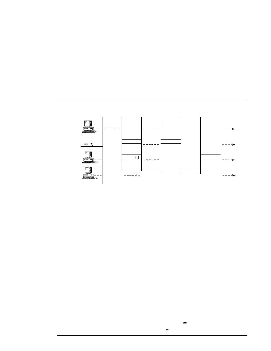
SECTION
/2.1
RANDOM ACCESS
369
Slotted ALOHA
Pure ALOHA has a vulnerable time of 2 x
T
fr .
This is so because there is no rule that
defines when the station can send. A station may send soon after another station has
started or soon before another station has finished. Slotted ALOHA was invented to
improve the efficiency of pure ALOHA.
In slotted ALOHA we divide the time into slots of T
fr
s and force the station to
send only at the beginning of the time slot. Figure 12.6 shows an example of frame
collisions in slotted ALOHA.
Figure 12.6
Frames in a slotted ALOHA network
Collision
Collision
duration
duration
Station]
Frame
1.]
Frame 1.2
--------------
- - - - - -
Time
Station 2
Frame 2.1
Frame 2.2
------
- - - - - -
- - - - - -
Time
Station 3
Frame
Frame 3.2
------
.....
-------
- - - - - - -
Time
Station 4
Frame 4.1
Frame 4.2
------
- - - - - -
- - - - - -
Time
Slot
1
510t2
Slot 3
510t4
Slot 5
Slot 6
Because a station is allowed to send only at the beginning of the synchronized time
slot, if a station misses this moment, it must wait until the beginning of the next time
slot. This means that the station which started at the beginning of this slot has already
finished sending its frame. Of course, there is still the possibility of collision if two sta-
tions try to send at the beginning of the same time slot. However, the vulnerable time is
now reduced to one-half, equal to
T
fr
Figure 12.7 shows the situation.
Figure 12.7 shows that the vulnerable time for slotted ALOHA is one-half that of
pure ALOHA.
Slotted ALOHA vulnerable time
=
T
fr
Throughput
It
can be proved that the average number of successful transmissions for
slotted ALOHA is
S
=
G x
e-
G
.
The maximum throughput
Smax
is 0.368, when G
=
1.
In other words, if a frame is generated during one frame transmission time, then 36.8
percent of these frames reach their destination successfully. This result can be expected
because the vulnerable time is equal to the frame transmission time. Therefore, if a sta-
tion generates only one frame in this vulnerable time (and no other station generates a
frame during this time), the frame will reach its destination successfully.
The throughput for slotted ALOHA is
S
G x
e
-G.
The maximum throughput
Smax
0.368 when G
=
1.
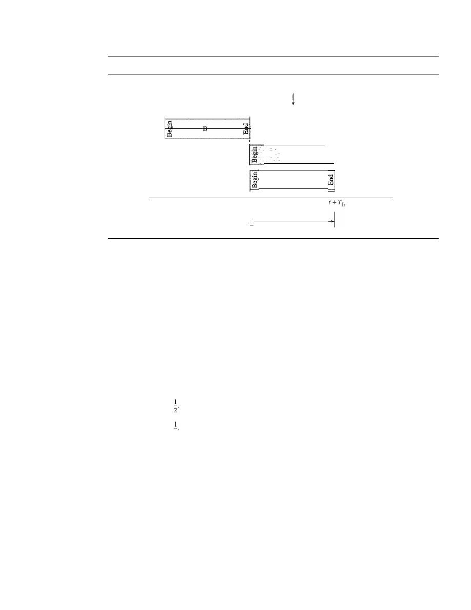
370
CHAPTER
12
MULTIPLE ACCESS
Figure 12.7
Vulnerable time for slotted ALOHA protocol
A collides with C
r
I
f
c
I,
Vulnerable time
=
T
fr
Time
Example 12.4
A slotted ALOHA network transmits 200-bit frames using a shared channel with a 200-kbps
bandwidth. Find the throughput if the system (all stations together) produces
a. 1000 frames per second
b. 500 frames per second
c. 250 frames per second
Solution
This situation is similar to the previous exercise except that the network is using slotted ALOHA
instead of pure ALOHA. The frame transmission time is
200/200
kbps or 1 ms.
a. In this case G is 1. So S
=
G x e-
G
or
S
=
0.368 (36.8 percent). This means that the
throughput is 1000 x 0.0368
=
368 frames. Only 368 out of 1000 frames will probably
survive. Note that this is the maximum throughput case, percentagewise.
b. Here G is
In this case S
=
G x e-
G
or S
=
0.303 (30.3 percent). This means that the
throughput is 500 x 0.0303
=
151. Only 151 frames out of 500 will probably survive.
c. Now Gis
In this case S
=
G x e-
G
or S
=
0.195 (19.5 percent). This means that the
throughput
4
is 250 x 0.195
=
49. Only 49 frames out of 250 will probably survive.
Carrier Sense Multiple Access (CSMA)
To minimize the chance of collision and, therefore, increase the performance, the CSMA
method was developed. The chance of collision can be reduced if a station senses the
medium before trying to use it. Carrier sense multiple access (CSMA) requires that each
station first listen to the medium (or check the state of the medium) before sending. In other
words, CSMA is based on the principle "sense before transmit" or "listen before talk."
CSMA can reduce the possibility of collision, but it cannot eliminate it. The reason
for this is shown in Figure
12.8,
a space and time model of a CSMA network. Stations
are connected to a shared channel (usually a dedicated medium).
The possibility of collision still exists because of propagation delay; when a station
sends a frame, it still takes time (although very short) for the first bit to reach every station
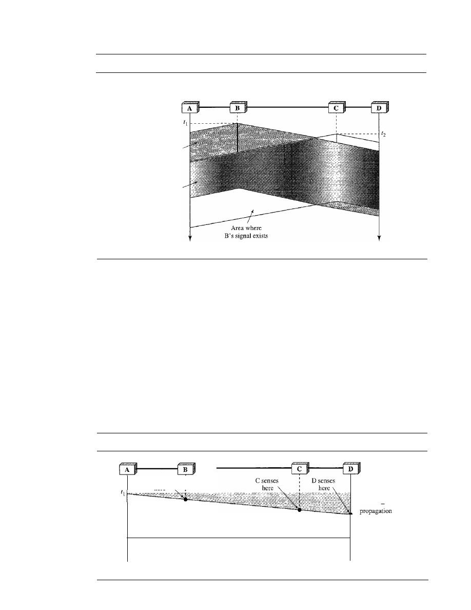
SECTION 12.1
RANDOM ACCESS
371
Figure 12.8
Space/time model of the collision in CSMA
B starts
at time
11
C starts
at time
12
Area where
A's signal exists
Area where
both signals exist
Time
Time
and for every station to sense it. In other words, a station may sense the medium and find
it idle, only because the first bit sent by another station has not yet been received.
At time
tI'
station B senses the medium and finds it idle, so it sends a frame. At time
t2 (t2> tI)'
station C senses the medium and finds it idle because, at this time, the first
bits from station B have not reached station
C.
Station C also sends a frame. The two
signals collide and both frames are destroyed.
Vulnerable Time
The vulnerable time for CSMA is the propagation time
T
p .
This is the time needed for
a signal to propagate from one end of the medium to the other. When a station sends a
frame, and any other station tries to send a frame during this time, a collision will
result. But if the first bit of the frame reaches the end of the medium, every station will
already have heard the bit and will refrain from sending. Figure 12.9 shows the worst
Figure 12.9
Vulnerable time in CSMA
B senses
here
Frame propagation
Time
]
Vulnerable time
time
Time
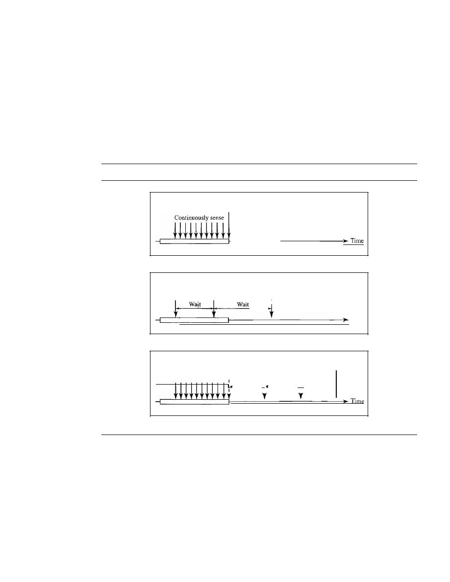
372
CHAPTER
12
MULTIPLE ACCESS
case. The leftmost station A sends a frame at time
tl'
which reaches the rightmost sta-
tion D at time
tl
+
T
p .
The gray area shows the vulnerable area in time and space.
Persistence Methods
What should a station do if the channel is busy? What should a station do if the channel
is idle? Three methods have been devised to answer these questions: the I-persistent
method, the nonpersistent method, and the p-persistent method. Figure 12.10 shows the
behavior of three persistence methods when a station finds a channel busy.
Figure 12.10
Behavior of three persistence methods
Sense
and transmit
Busy
3.
I-persistent
Sense
Sense
and transmit
Sense
I
Time
Busy
b. Nonpersistent
Transmit
I
I
I
Probability outcome
does not allow transmission.
I
I
I
Continuously sense
I
I
I
Time slot
I
Time slot
I
Time slot
.1
.1.
Busy
c. p-persistent
Figure 12.11 shows the flow diagrams for these methods.
I-Persistent
The
I-persistent method is simple and straightforward. In this method,
after the station finds the line idle, it sends its frame immediately (with probability I).
This method has the highest chance of collision because two or more stations may find
the line idle and send their frames immediately. We will see in Chapter 13 that Ethernet
uses this method.
Nonpersistent
In the nonpersistent method, a station that has a frame to send
senses the line. If the line is idle, it sends immediately.
If
the line is not idle, it waits a
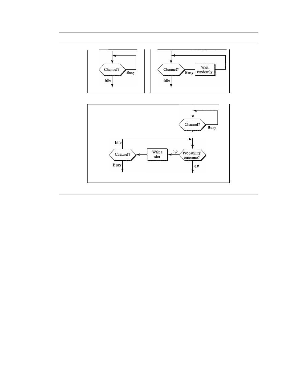
SECTION 12.1
RANDOM ACCESS
373
Figure 12.11
Flow diagram for three persistence methods
Station can transmit.
a.
1-
persistent
Use back-off process
as though collision occurred.
c. p-persistent
Station can transmit.
b. Nonpersistent
Idle
Station can transmit.
random amount of time and then senses the line again. The nonpersistent approach
reduces the chance of collision because it is unlikely that two or more stations will wait
the same amount of time and retry to send simultaneously. However, this method
reduces the efficiency of the network because the medium remains idle when there may
be stations with frames to send.
p-Persistent
The p-persistent method
is used if the channel has time slots with a slot
duration equal to or greater than the maximum propagation time. The p-persistent approach
combines the advantages of the other two strategies. It reduces the chance of collision and
improves efficiency.
In
this method, after the station finds the line idle it follows these steps:
1. With probability
p,
the station sends its frame.
2. With probability
q
=
1 -
p,
the station waits for the beginning of the next time slot
and checks the line again.
a. If the line is idle, it goes to step 1.
b.
If
the line is busy, it acts as though a collision has occurred and uses the back-
off procedure.
Carrier Sense Multiple Access with Collision Detection (CSMA/CD)
The CSMA method does not specify the procedure following a collision. Carrier sense
multiple access with collision detection (CSMA/CD) augments the algorithm to handle
the collision.
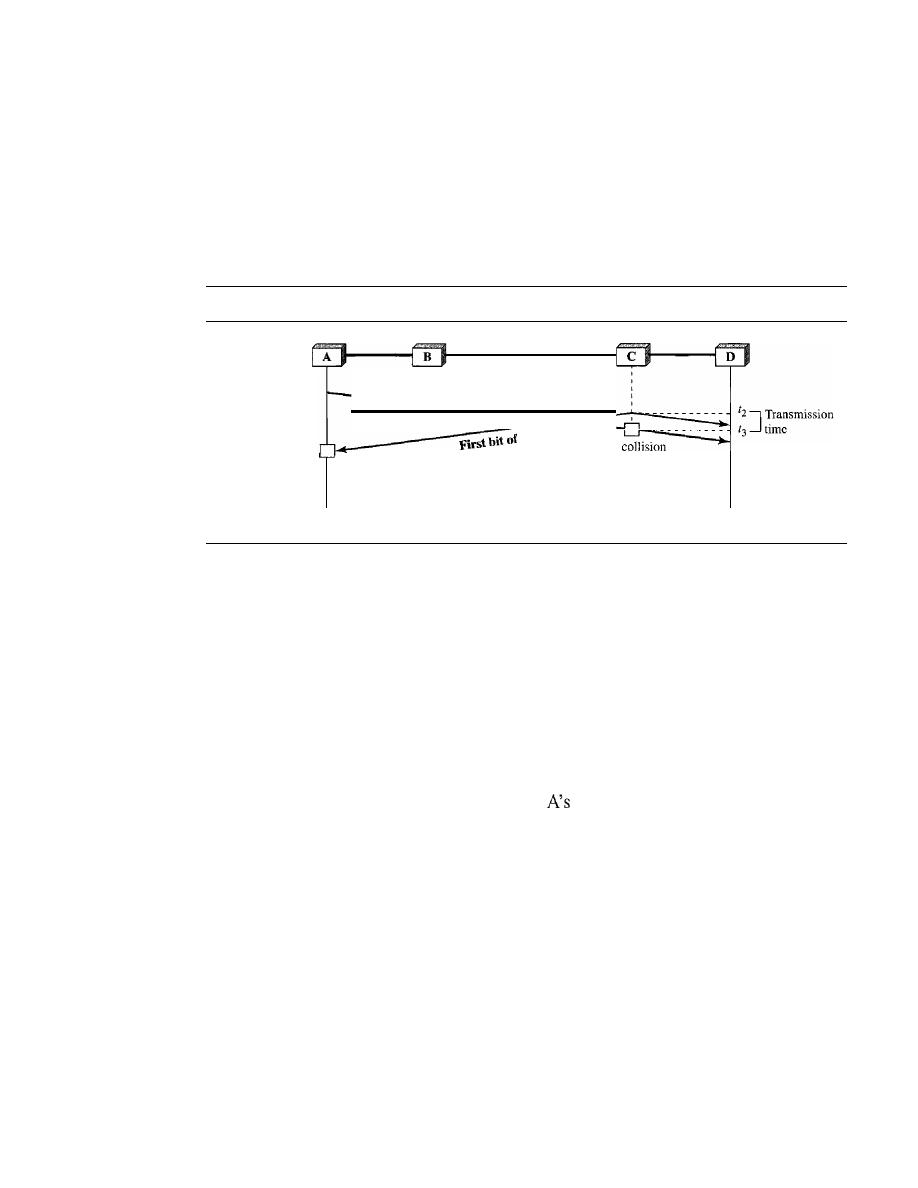
374
CHAPTER
12
MULTIPLEACCESS
In this method, a station monitors the medium after it sends a frame to see if the
transmission was successful. If so, the station is finished.
If,
however, there is a colli-
sion, the frame is sent again.
To better understand CSMA/CD, let us look at the first bits transmitted by the two
stations involved in the collision. Although each station continues to send bits in the
frame until it detects the collision, we show what happens as the first bits collide. In
Figure 12.12, stations A and C are involved in the collision.
Figure 12.12
Collision of the first bit in CSMAlCD
First bit
of
A
C
C's
detection and
Collision
abortion
occurs
A's collision
detection
and abortion
[
t
l
Transmission
time
14
Time
Time
At time
t
1,
station A has executed its persistence procedure and starts sending the
bits of its frame. At time
t2,
station C has not yet sensed the first bit sent by A. Station C
executes its persistence procedure and starts sending the bits in its frame, which propa-
gate both to the left and to the right. The collision occurs sometime after time
t2'
Station C
detects a collision at time
t3
when it receives the first bit of A's frame. Station C immedi-
ately (or after a short time, but we assume immediately) aborts transmission. Station A
detects collision at time
t4
when it receives the first bit of C's frame; it also immediately
aborts transmission. Looking at the figure, we see that A transmits for the duration
t4 - tl;
C transmits for the duration
t3 - t2'
Later we show that, for the protocol to work, the
length of any frame divided
by
the bit rate in this protocol must be more than either of
these durations. At time
t4,
the transmission of
frame, though incomplete, is aborted;
at time
t
3 ,
the transmission of B's frame, though incomplete, is aborted.
Now that we know the time durations for the two transmissions, we can show a
more complete graph in Figure 12.13.
Minimum Frame Size
For
CSMAlCD
to work, we need a restriction on the frame size. Before sending the last
bit of the frame, the sending station must detect a collision, if any, and abort the transmis-
sion. This is so because the station, once the entire frame is sent, does not keep a copy of
the frame and does not monitor the line for collision detection. Therefore, the frame trans-
mission time
T
fr
must be at least two times the maximum propagation time
T
p .
To under-
stand the reason, let us think about the worst-case scenario.
If
the two stations involved in
a collision are the maximum distance apart, the signal from the first takes time
T
p
to reach
the second, and the effect of the collision takes another time
T
p
to reach the first. So the
requirement is that the first station must still be transmitting after
2T
p .
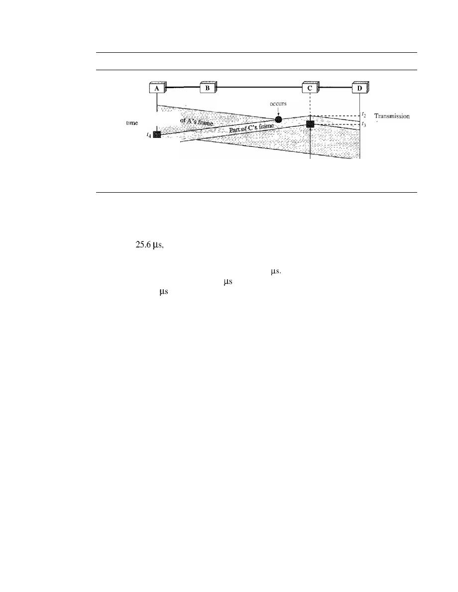
SECTION 12.1
RANDOM ACCESS
375
Figure 12.13
Collision and abortion in CSMAlCD
Collision
Transmission
[1[
]
13
tIme
A detects
collision and
aborts
Time
C detects
collision
and aborts
Time
Example 12.5
A network using
CSMA/CD has a bandwidth of 10 Mbps.
If
the maximum propagation time
(including the delays in the devices and ignoring the time needed to send a jamming signal, as we
see later) is
what is the minimum size of the frame?
Solution
The frame transmission time is
T
fr
=
2 x
T
p
=
51.2
This means, in the worst case, a station
needs to transmit for a period of
51.2
to detect the collision. The minimum size of the frame
is 10 Mbps x 51.2
=
512 bits or 64 bytes. This is actually the minimum size of the frame for
Standard Ethernet, as we will see in Chapter 13.
Procedure
Now let us look at the flow diagram for CSMAlCD in Figure 12.14. It is similar to the
one for the ALOHA protocol, but there are differences.
The first difference is the addition of the persistence process. We need to sense the
channel before we start sending the frame by using one of the persistence processes we
discussed previously (nonpersistent, I-persistent, or p-persistent). The corresponding
box can be replaced by one of the persistence processes shown in Figure 12.11.
The second difference is the frame transmission. In ALOHA, we first transmit the
entire frame and then wait for an acknowledgment. In CSMA/CD, transmission and
collision detection is a continuous process. We do not send the entire frame and then
look for a collision. The station transmits and receives continuously and simultaneously
(using two different ports). We use a loop to show that transmission is a continuous
process. We constantly monitor in order to detect one of two conditions: either trans-
mission is finished or a collision is detected. Either event stops transmission. When we
come out of the loop, if a collision has not been detected, it means that transmission is
complete; the entire frame is transmitted. Otherwise, a collision has occurred.
The third difference is the sending of a short jamming signal that enforces the colli-
sion in case other stations have not yet sensed the collision.
Energy Level
We can say that the level of energy in a channel can have three values: zero, normal,
and abnormal. At the zero level, the channel is idle. At the normal level, a station has
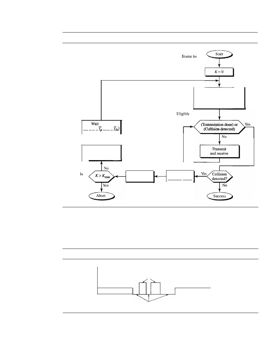
376
CHAPTER 12
MULTIPLE ACCESS
Figure 12.14
Flow diagramfor the CSMAlCD
K: Number of attempts
T
p :
Maximum propagation time
T
fr :
Average transmission time for a frame
Tn:
Back-off time
Station has
a
send
Apply one of the
persistence methods
(I-persistent, nonpersistent,
or p-persistent)
TBtime
(T
B
=
R x
or R
X
Choose a random
number
R
between
o
and 2
K
- l
K
ma\
normally 15
K=K+I
fur transmission
Send
a
jamming signal
successfully captured the channel and is sending its frame. At the abnormal level, there
is a collision and the level of the energy is twice the normal level. A station that has a
frame to send or is sending a frame needs to monitor the energy level to determine if
the channel is idle, busy, or in collision mode. Figure 12.15 shows the situation.
Figure 12.15
Energy level during transmission, idleness, or collision
Energy
Collision
Frame transmission
Idle
Frame transmission
Time
Throughput
The throughput of CSMAlCD is greater than that of pure or slotted ALOHA. The maxi-
mum throughput occurs at a different value of G and is based on the persistence method
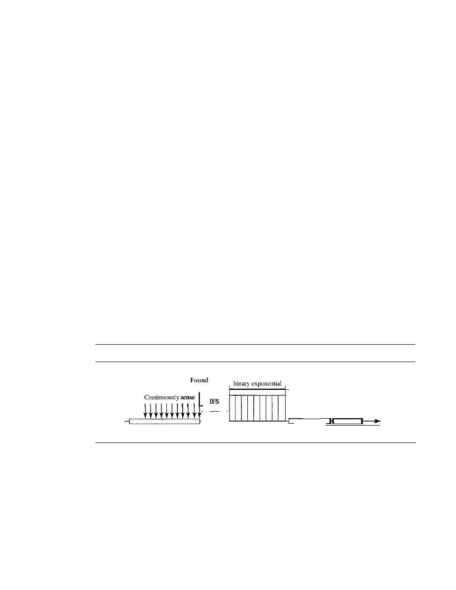
SECTION
12.1
RANDOM ACCESS
377
and the value of
p
in the p-persistent approach. For I-persistent method the maximum
throughput is around 50 percent when G
=
1. For nonpersistent method, the maximum
throughput can go up to 90 percent when G is between 3 and 8.
Carrier Sense Multiple Access with
Collision Avoidance (CSMA/CA)
The basic idea behind
CSMA/CD
is that a station needs to be able to receive while
transmitting to detect a collision. When there is no collision, the station receives one
signal: its own signal. When there is a collision, the station receives two signals: its own
signal and the signal transmitted by a second station. To distinguish between these two
cases, the received signals in these two cases must be significantly different. In other
words, the signal from the second station needs to add a significant amount of energy to
the one created by the first station.
In a wired network, the received signal has almost the same energy as the sent sig-
nal because either the length of the cable is short or there are repeaters that amplify the
energy between the sender and the receiver. This means that in a collision, the detected
energy almost doubles.
However, in a wireless network, much of the sent energy is lost in transmission. The
received signal has very little energy. Therefore, a collision may add only 5 to 10 percent
additional energy. This is not useful for effective collision detection.
We need to avoid collisions on wireless networks because they cannot be detected.
Carrier sense multiple access with collision avoidance
(CSMAlCA)
was invented for this
network. Collisions are avoided through the use of CSMAICA's three strategies: the inter-
frame space, the contention window, and acknowledgments, as shown in Figure 12.16.
Figure 12.16
Timing in CSMAICA
Size:
idle
exponential
.
Busy
Contention window
Send frame
Time-out
Time
Interframe Space (IFS)
First, collisions are avoided by deferring transmission even if the channel is found idle.
When an idle channel is found, the station does not send immediately.
It
waits for a
period of time called the interframe space or IFS. Even though the channel may
appear idle when it is sensed, a distant station may have already started transmitting.
The distant station's signal has not yet reached this station. The IFS time allows the
front of the transmitted signal by the distant station to reach this station.
If
after the IFS
time the channel is still idle, the station can send, but it still needs to wait a time equal
to the contention time (described next). The IFS variable can also be used to prioritize

378
CHAPTER
12
MULTIPLE ACCESS
stations or frame types. For example, a station that is assigned a shorter IFS has a
higher priority.
In CSMAlCA, the IFS can also be used to define
the priority of a station or a frame.
Contention Window
The contention window is an amount of time divided into slots. A station that is ready
to send chooses a random number of slots as its wait time. The number of slots in the
window changes according to the binary exponential back-off strategy. This means that
it is set to one slot the first time and then doubles each time the station cannot detect an
idle channel after the IFS time. This is very similar to the p-persistent method except
that a random outcome defines the number of slots taken by the waiting station. One
interesting point about the contention window is that the station needs to sense the
channel after each time slot. However, if the station finds the channel busy, it does not
restart the process; it just stops the timer and restarts it when the channel is sensed as
idle. This gives priority to the station with the longest waiting time.
In CSMAlCA, if the station finds the channel busy,
it does not restart the timer of the contention window;
it stops the timer and restarts it when the channel becomes idle.
Acknowledgment
With all these precautions, there still may be a collision resulting in destroyed data.
In addition, the data may be corrupted during the transmission. The positive acknowl-
edgment and the time-out timer can help guarantee that the receiver has received the
frame.
Procedure
Figure 12.17 shows the procedure. Note that the channel needs to be sensed before and
after the IFS. The channel also needs to be sensed during the contention time. For each
time slot of the contention window, the channel is sensed.
If
it is found idle, the timer
continues; if the channel is found busy, the timer is stopped and continues after the
timer becomes idle again.
CSMAICA and Wireless Networks
CSMAICA
was mostly intended for use in wireless networks. The procedure described
above, however, is not sophisticated enough to handle some particular issues related to
wireless networks, such as hidden terminals or exposed terminals. We will see how
these issues are solved by augmenting the above protocol with hand-shaking features.
The use of
CSMNCA
in wireless networks will be discussed in Chapter 14.
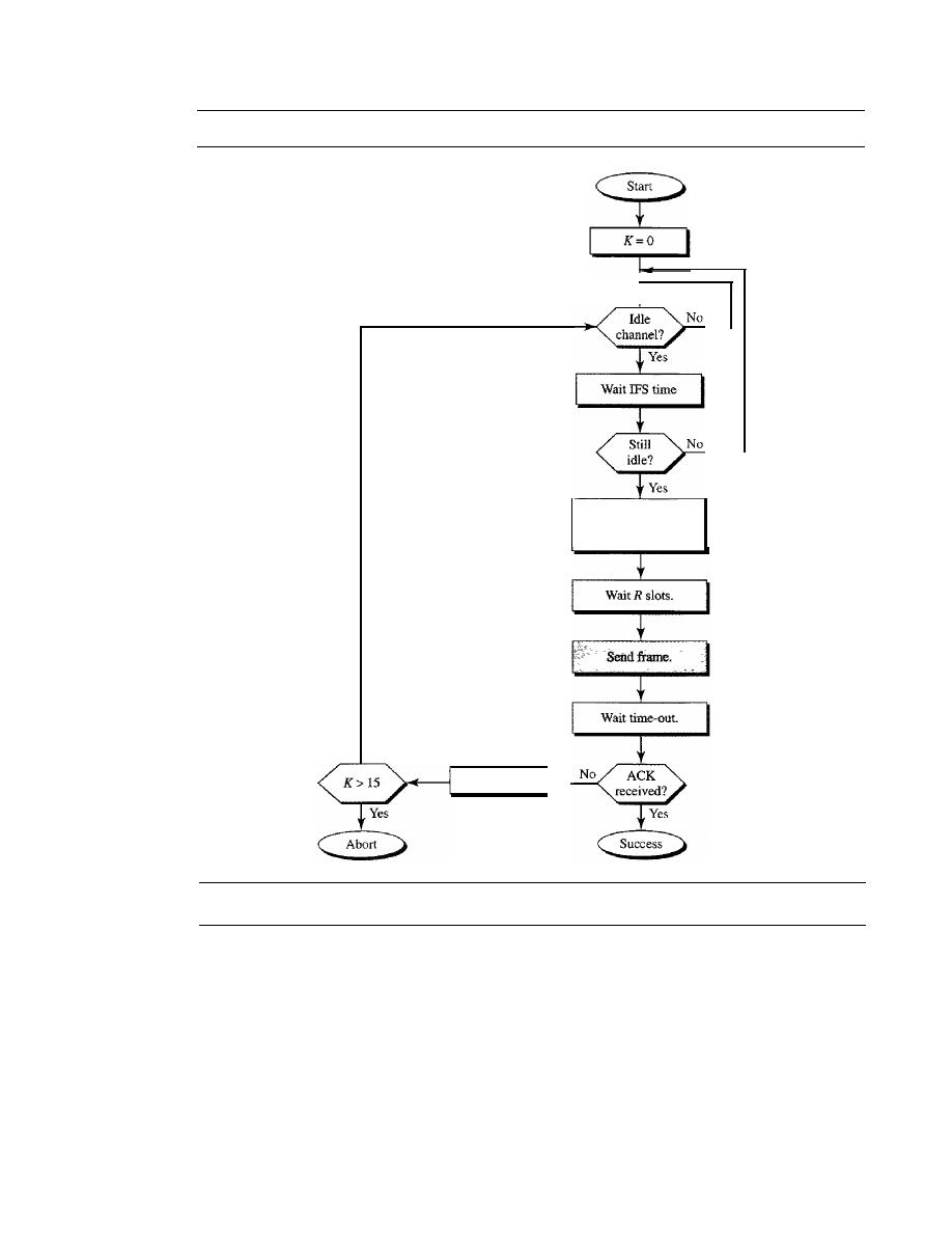
SECTION
12.2
CONTROLLED ACCESS
379
Figure 12.17
Flow diagramfor CSMAICA
12.2
Contention window
size is ZK - 1.
After each slot, if idle,
continue; if busy, halt and
continue when idle.
No
K=K+I
CONTROLLED
ACCESS
Choose a random
number
R between
o
and
ZK -
I
In
controlled access,
the stations consult one another to find which station has the right
to send. A station cannot send unless it has been authorized
by
other stations. We discuss
three popular controlled-access methods.
Reservation
In the
reservation
method, a station needs to make a reservation before sending data.
Time is divided into intervals. In each interval, a reservation frame precedes the data
frames sent in that interval.
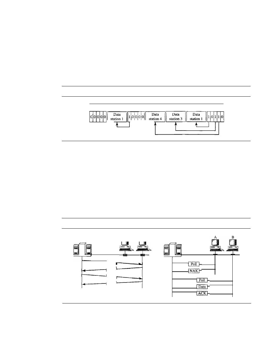
380
CHAPTER
12
MULTIPLE ACCESS
If
there are
N
stations in the system, there are exactly
N
reservation minislots in the
reservation frame. Each minislot belongs to a station. When a station needs to send a
data frame, it makes a reservation in its own minislot. The stations that have made res-
ervations can send their data frames after the reservation frame.
Figure 12.18 shows a situation with five stations and a five-minislot reservation
frame. In the first interval, only stations 1, 3, and 4 have made reservations. In the sec-
ond interval, only station 1 has made a reservation.
Figure 12.18
Reservation access method
1 2 345
1 2 345
1 2345
Reservation
frame
Polling
Polling works with topologies in which one device is designated as a primary station
and the other devices are
secondary stations. All data exchanges must be made
through the primary device even when the ultimate destination is a secondary device.
The primary device controls the link; the secondary devices follow its instructions.
It
is up to the primary device to determine which device is allowed to use the channel at
a given time. The primary device, therefore, is always the initiator of a session (see
Figure 12.19).
Figure 12.19
Select and poll functions in polling access method
Poll
ACK
Primary
Primary
SEL
ACK
Select
Data
If
the primary wants to receive data, it asks the secondaries if they have anything to
send; this is called poll function. If the primary wants to send data, it tells the secondary
to get ready to receive; this is called select function.

SECTION
12.2
CONTROLLED ACCESS
381
Select
The
select
function is used whenever the primary device has something to send.
Remember that the primary controls the link.
If
the primary is neither sending nor
receiving data, it knows the link is available.
If
it has something to send, the primary device sends it. What it does not know,
however, is whether the target device is prepared to receive. So the primary must alert
the secondary to the upcoming transmission and wait for an acknowledgment of the
secondary's ready status. Before sending data, the primary creates and transmits a
select (SEL) frame, one field of which includes the address of the intended secondary.
Poll
The
poll
function is used by the primary device to solicit transmissions from the sec-
ondary devices. When the primary is ready to receive data, it must ask (poll) each
device in turn if it has anything to send. When the first secondary is approached, it
responds either with a NAK frame if it has nothing to send or with data (in the form of
a data frame) if it does.
If
the response is negative (a NAK frame), then the primary
polls the next secondary in the same manner until it finds one with data to send. When
the response is positive (a data frame), the primary reads the frame and returns an
acknowledgment (ACK frame), verifying its receipt.
Token Passing
In the
token-passing method, the stations in a network are organized in a logical ring.
In other words, for each station, there is a
predecessor
and a
successor.
The predecessor
is the station which is logically before the station in the ring; the successor is the station
which is after the station in the ring. The current station is the one that is accessing the
channel now. The right to this access has been passed from the predecessor to the cur-
rent station. The right will be passed to the successor when the current station has no
more data to send.
But how is the right to access the channel passed from one station to another? In
this method, a special packet called a
token circulates through the ring. The posses-
sion of the token gives the station the right to access the channel and send its data.
When a station has some data to send, it waits until it receives the token from its pre-
decessor.
It
then holds the token and sends its data. When the station has no more data
to send, it releases the token, passing it to the next logical station in the ring. The sta-
tion cannot send data until it receives the token again in the next round. In this process,
when a station receives the token and has no data to send, it just passes the data to the
next station.
Token management is needed for this access method. Stations must be limited in
the time they can have possession of the token. The token must be monitored to ensure
it has not been lost or destroyed. For example, if a station that is holding the token fails,
the token will disappear from the network. Another function of token management is
to assign priorities to the stations and to the types of data being transmitted. And finally,
token management is needed to make low-priority stations release the token to high-
priority stations.
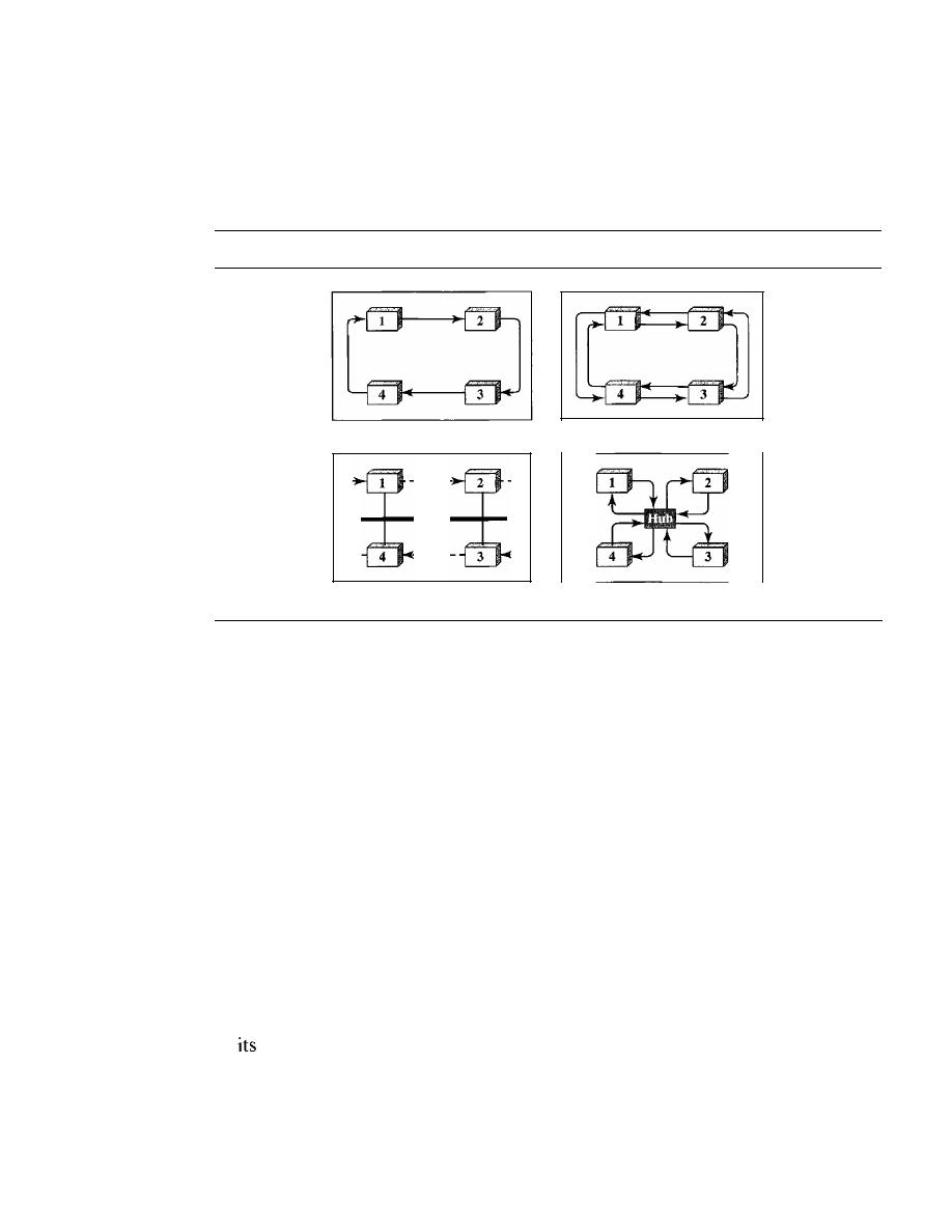
382
CHAPTER
12
MULTIPLE ACCESS
Logical Ring
In a token-passing network, stations do not have to be physically connected in a ring;
the ring can be a logical one. Figure 12.20 show four different physical topologies that
can create a logical ring.
Figure 12.20
Logical ring and physical topology in token-passing access method
a. Physical ring
1
1
1
1
1
1
1
1-
c. Bus ring
b. Dual ring
d. Star ring
In the physical ring topology, when a station sends the token to its successor, the
token cannot be seen by other stations; the successor is the next one in line. This means
that the token does not have to have the address of the next successor. The problem with
this topology is that if one of the links-the medium between two adjacent stations-
fails, the whole system fails.
The dual ring topology uses a second (auxiliary) ring which operates in the reverse
direction compared with the main ring. The second ring is for emergencies only (such as
a spare tire for a car). If one of the links in the main ring fails, the system automatically
combines the two rings to form a temporary ring. After the failed link is restored, the
auxiliary ring becomes idle again. Note that for this topology to work, each station needs
to have two transmitter ports and two receiver ports. The high-speed Token Ring networks
called FDDI (Fiber Distributed Data Interface) and CDDI (Copper Distributed Data
Interface) use this topology.
In the bus ring topology, also called a token bus, the stations are connected to a sin-
gle cable called a bus. They, however, make a logical ring, because each station knows
the address of its successor (and also predecessor for token management purposes).
When a station has finished sending its data, it releases the token and inserts the address
of
successor in the token. Only the station with the address matching the destination
address of the token gets the token to access the shared media. The Token Bus LAN,
standardized by IEEE, uses this topology.
In a star ring topology, the physical topology is a star. There is a hub, however, that
acts as the connector. The wiring inside the hub makes the ring; the stations are con-
nected to this ring through the two wire connections. This topology makes the network
SECTION
12.3
CHANNELIZATION
383
less prone to failure because if a link goes down, it will be bypassed by the hub and the
rest of the stations can operate. Also adding and removing stations from the ring is easier.
This topology is still used in the Token Ring LAN designed by IBM.
12.3
CHANNELIZATION
Channelization is a multiple-access method in which the available bandwidth of a link
is shared in time, frequency, or through code, between different stations. In this section,
we discuss three channelization protocols: FDMA, TDMA, and CDMA.
We see the application of all these methods in Chapter 16
when we discuss cellular phone systems.
Frequency-Division Multiple Access (FDMA)
In frequency-division multiple access (FDMA), the available bandwidth is divided
into frequency bands. Each station is allocated a band to send its data. In other words,
each band is reserved for a specific station, and it belongs to the station all the time.
Each station also uses a bandpass filter to confine the transmitter frequencies. To pre-
vent station interferences, the allocated bands are separated from one another by small
guard bands.
Figure 12.21 shows the idea of FDMA.
Figure
12.21
Frequency-division multiple access (FDMA)
Data
Data
Silent
•••
t
--------
_ _ _ _ _ _ _ .J
_ _ _ _ _ _ _ .J
• • •
--------
t
Data
" I
--------
_ _ _ _ _ _ _
• • •
- - - - - - - -
_ _ _ _ _ _ _
t
Common
channel
Data
In FDMA, the available bandwidth of the common channel
is divided into bands that are separated by guard bands.
384
CHAPTER
12
MULTIPLE ACCESS
FDMA specifies a predetermined frequency band for the entire period of commu-
nication. This means that stream data (a continuous flow of data that may not be pack-
etized) can easily be used with FDMA. We will see in Chapter 16 how this feature can
be used in cellular telephone systems.
We need to emphasize that although FDMA and FDM conceptually seem similar,
there are differences between them. FDM, as we saw in Chapter 6, is a physical layer
technique that combines the loads from low-bandwidth channels and transmits them by
using a high-bandwidth channel. The channels that are combined are low-pass. The
multiplexer modulates the signals, combines them, and creates a bandpass signal. The
bandwidth of each channel is shifted by the multiplexer.
FDMA, on the other hand, is an access method in the data link layer. The data link
layer in each station tells its physical layer to make a bandpass signal from the data
passed to it. The signal must be created in the allocated band. There is no physical mul-
tiplexer at the physical layer. The signals created at each station are automatically
bandpass-filtered. They are mixed when they are sent to the common channel.
Time-Division Multiple Access (TDMA)
In
time-division multiple access (TDMA),
the stations share the bandwidth of the
channel in time. Each station is allocated a time slot during which it can send data.
Each station transmits its data in is assigned time slot. Figure 12.22 shows the idea
behind TDMA.
Figure 12.22
Time-division multiple access (TDMA)
Data
Data
f
-I,--
I:: :: I···
I
II
I,
r
f
II
,
"
,
II
I · · ·
t
I
'I
I
Data
Common
channel
f
I
I
: • • •
,
'
Silent
f
II
II
IJ
II
I
II
II
I
Data
The main problem with TDMA lies in achieving synchronization between the different
stations. Each station needs to know the beginning of its slot and the location of its slot.
This may be difficult because of propagation delays introduced in the system if the sta-
tions are spread over a large area. To compensate for the delays, we can insert
guard

SECTION
12.3
CHANNELIZATION
385
times.
Synchronization is normally accomplished by having some synchronization bits
(normally refened to as preamble bits) at the beginning of each slot.
In TDMA, the bandwidth is just one channel that is
timeshared between different stations.
We also need to emphasize that although TDMA and TDM conceptually seem the
same, there are differences between them. TDM, as we saw in Chapter 6, is a physical
layer technique that combines the data from slower channels and transmits them by
using a faster channel. The process uses a physical multiplexer that interleaves data
units from each channel.
TDMA, on the other hand, is an access method in the data link layer. The data link
layer in each station tells its physical layer to use the allocated time slot. There is no
physical multiplexer at the physical layer.
Code-Division Multiple Access (CDMA)
Code-division multiple access (CDMA) was conceived several decades ago. Recent
advances in electronic technology have finally made its implementation possible.
CDMA differs from FDMA because only one channel occupies the entire bandwidth of
the link.
It
differs from TDMA because all stations can send data simultaneously; there
is no timesharing.
In CDMA, one channel carries all transmissions simultaneously.
Analogy
Let us first give an analogy. CDMA simply means communication with different codes.
For example, in a large room with many people, two people can talk in English if
nobody else understands English. Another two people can talk in Chinese if they are
the only ones who understand Chinese, and so on. In other words, the common channel,
the space of the room in this case, can easily allow communication between several
couples, but in different languages (codes).
Idea
Let us assume we have four stations 1, 2, 3, and 4 connected to the same channel. The
data from station 1 are
d
l ,
from station 2 are
d
2,
and so on. The code assigned to the
first station is
cI,
to the second is
c2,
and so on. We assume that the assigned codes have
two properties.
1.
If
we multiply each code by another, we get O.
2. If we multiply each code by itself, we get 4 (the number of stations).
With these two properties in mind, let us see how the above four stations can send data
using the same common channel, as shown in Figure 12.23.
Station 1 mUltiplies (a special kind of multiplication, as we will see) its data by its
code to get d
l . Cl'
Station 2 multiplies its data by its code to get
d
2 . c2'
And so on. The
386
CHAPTER
12
MULTIPLE ACCESS
Figure 12.23
Simple idea of communication with code
I
d,' (',
+
d
2 •
c2
+
d
3 •
('3
+
d
4 •
('4
I
Data
Common
channel
data that go on the channel are the sum of all these terms, as shown in the box. Any
station that wants to receive data from one of the other three multiplies the data on the
channel by the code of the sender. For example, suppose stations 1 and 2 are talking to
each other. Station 2 wants to hear what station I is saying.
It
multiplies the data on the
channel by
cl'
the code of station 1.
Because
(cl . cl)
is 4, but
(c2 .
cI),
(c3 .
cI),
and
(c4 .
cl)
are all Os, station 2 divides
the result by 4 to get the data from station 1.
data
=
(d}
Cj
+
d
z . Cz
+
d
3 . C3
+
d
4 . c4) . Cl
=
d
j •
Cl .
Cj
+
d
z.
Cz . Cl
+
d
3 . C3 .
Cl
+
d
4 . C4'
CI
=
4
X
d
1
Chips
CDMA is based on coding theory. Each station is assigned a code, which is a sequence
of numbers called chips, as shown in Figure 12.24. The codes are for the previous
example.
Figure 12.24
Chip sequences
C
I
[+1 +1
+1
+11
I
1[+1 -1 +1
-I)
I
I
[+1 +\
-I - 11
I
I
[+\
-1 -1 +IJ
I
Later in this chapter we show how we chose these sequences. For now, we need to
know that we did not choose the sequences randomly; they were carefully selected.
They are called
orthogonal sequences
and have the following properties:
1. Each sequence is made of
N
elements, where
N
is the number of stations.
SECTION
12.3
CHANNELIZATION
387
2.
If
we multiply a sequence by a number, every element in the sequence is multiplied
by that element. This is called multiplication of a sequence by a scalar. For example,
2. [+1 +1-1-1]=[+2+2-2-2]
3. If we multiply two equal sequences, element by element, and add the results, we
get
N,
where
N
is the number of elements in the each sequence. This is called the
inner product of two equal sequences. For example,
[+1 +1-1
[+1 +1 -1 -1] = 1 + 1 + 1 + 1 = 4
4.
If
we multiply two different sequences, element by element, and add the results,
we get O. This is called inner product of two different sequences. For example,
[+1 +1
-1] •
[+1 +1 +1
+1]
= 1 + 1
1
1 = 0
5. Adding two sequences means adding the corresponding elements. The result is
another sequence. For example,
[+1+1-1-1]+[+1+1+1+1]=[+2+2 00]
Data Representation
We follow these rules for encoding:
If
a station needs to send a 0 bit, it encodes it as
-1;
if it needs to send a 1 bit, it encodes it as
+
1. When a station is idle, it sends no signal,
which is interpreted as a O. These are shown in Figure 12.25.
Figure 12.25
Data representation in CDMA
I
Data bit 0
-I
I
I
Data bit I
+
1
I
Silence
0
I
Encoding and Decoding
As a simple example, we show how four stations share the
link during a I-bit interval.
The procedure can easily be repeated for additional intervals. We assume that stations 1
and 2 are sending a 0 bit and channel 4 is sending a 1 bit. Station 3 is silent. The data at
the sender site are translated to
-1, -1,
0, and
+
1. Each station multiplies the correspond-
ing number by its chip (its orthogonal sequence), which is unique for each station. The
result is a new sequence which is sent to the channel. For simplicity, we assume that all
stations send the resulting sequences at the same time. The sequence on the channel is
the sum of all four sequences as defined before. Figure 12.26 shows the situation.
Now imagine station 3, which we said is silent, is listening to station 2. Station 3 mul-
tiplies the total data on the channel by the code for station 2, which is
[+
1
-1
+
1 -1],
to get
[-1-1-3 +1]· [+1-1 +1-1] =-4/4 =-1
bit 1
388
CHAPTER 12
MULTIPLE ACCESS
Figure 12.26
Sharing channel in CDMA
Bit
a
Bit
a
C
1
1+1 +1 +1 +IJ
d
1
•
c
1
[-1 -I
-I -I]
C
2
1+1 -I
+1 -1]
[-1 -1
-3
+1]
Data
Common
channel
c
[+1 +1 -1 -11
C
1+1
-I
-1 +11
Silent
Bit
1
Signal Level
The process can be better understood if we show the digital signal produced by each
station and the data recovered at the destination (see Figure 12.27). The figure shows the
corresponding signals for each station (using NRZ-L for simplicity) and the signal that
is on the common channel.
Figure 12.27
Digital signal created by four stations in CDMA
BitO
1-1 -1 -I -I]
BitO
1-1 +1 -I +1]
Silent
[0
0
0
0]
Bit I
1+1
-I +1]
Data on the channel
Time
Time
Time
Time
Time
Figure 12.28 shows how station 3 can detect the data sent by station 2 by using the
code for station 2. The total data on the channel are multiplied (inner product opera-
tion) by the signal representing station 2 chip code to get a new signal. The station then
integrates and adds the area under the signal, to get the value -4, which is divided by 4
and interpreted as bit O.
SECTION 12.3
CHANNELIZATION
389
Figure 12.28
Decoding of the composite signal for one in CDMA
Data on the channel
Time
Station 2's code
[+1 -I
+1 -1]
Inner product result
Summing the values
Time
Time
Time
-4
-4/4
-I
BitO
Sequence Generation
To generate chip sequences, we use a
Walsh table,
which is a two-dimensional table with
an equal number of rows and columns, as shown in Figure 12.29.
Figure 12.29
General rule and examples of creating Walsh tables
a. Two basic rules
WI
=
+1
+1
+1
+1
+1
-1
+1
-1
W
4
=
+1
+1
-1
-1
W
z
=
+1
-1
+1
-1
-1
+1
b. Generation of WI'
W
z,
and
W
4
In the Walsh table, each row is a sequence of chips.
WI
for a one-chip sequence has
one row and one column. We can choose -lor + 1 for the chip for this trivial table (we
chose
+
1). According to Walsh, if we know the table for
N
sequences
W
N'
we can create
the table for
2N
sequences
W
2N,
as shown in Figure 12.29. The
W
N
with the overbar
W
N
stands for the complement of
W
N'
where each +1 is changed to -1 and vice versa.
Figure 12.29 also shows how we can create
W2
and
W4
from
WI'
After we select
WI, W2

390
CHAPTER
12
MULTIPLE ACCESS
can be made from four
W
j
's, with the last one the complement of
Wl'
After
W
2
is gener-
ated, W
4
can be made of four W
2
's,
with the last one the complement of W
2.
Of course,
W
s
is composed of four
W
4
's,
and so on. Note that after
W
N
is made, each station is
assigned a chip corresponding to a row.
Something we need to emphasize is that the number of sequences
N
needs to be a
power of 2. In other words, we need to have N
=
2
m
.
The number of sequences in a Walsh table needs to beN
=
2
m.
Example 12.6
Find the chips for a network with
a. Two stations
b. Four stations
Solution
We can use the rows of W
2
and W
4
in Figure 12.29:
a. For a two-station network, we have [+ 1 + 1] and [+ 1 -1].
b. For a four-station network we have [+1 +1 +1 +1], [+1 -1 +1 -1], [+1 +1 -1
and
[+1-1-1 +1].
Example 12.7
What is the number of sequences if we have 90 stations in our network?
Solution
The number of sequences needs to be
2
m
.
We need to choose
m
=
7 and
N
=
2
7
or 128. We can
then use 90 of the sequences as the chips.
Example 12.8
Prove that a receiving station can get the data sent by a specific sender if it multiplies the entire
data on the channel by the sender's chip code and then divides it by the number of stations.
Solution
Let us prove this for the first station, using our previous four-station example. We can say that the
data on the channel D
=
Cd
l . ("1
+
d
2 .
("2
+
d
3 .
("3
+
d
4 .
("4)'
The receiver which wants to get the
data sent by station I multiplies these data by
("I'
D .
("1
=
(d
1 •
("1
+ d
2 .
("2
+ d
3 .
("3
+ d
4 .
("4) . ("1
=
d
1 .
("1 . ("1
+
d
2 .
("2 . ("1
+
d
3 .
("3 . ("1
+
d
4 .
("4 . ("1
=
d
I X
N
+
d
2
X
0
+
d
3
X
0
+
d
4
X
0
=d
l
xN
When we divide the result by N, we get d
I'
12.4
RECOMMENDED READING
For more details about subjects discussed in this chapter, we recommend the following
books. The items in brackets [...
J
refer to the reference list at the end of the text.

SECTION
12.6
SUMMARY
391
Books
Multiple access is discussed in Chapter 4 of [Tan03], Chapter 16 of [Sta04], Chapter 6 of
[GW04], and Chapter 8 of [For03]. More advanced materials can be found in [KMK04].
12.5
KEY TERMS
I-persistent method
ALOHA
binary exponential backup
carrier sense multiple access (CSMA)
carrier sense multiple access with
collision avoidance
(CSMAlCA)
carrier sense multiple access with
collision detection
(CSMAlCD)
channelization
code-division multiple access (CDMA)
collision
contention
controlled access
frequency-division multiple access
(FDMA)
inner product
interframe space (IFS)
jamming signal
multiple access (MA)
nonpersistent method
orthogonal sequence
polling
p-persistent method
primary station
propagation time
pure ALOHA
random access
reservation
secondary station
slotted ALOHA
time-division multiple access
(TDMA)
token
token passing
vulnerable time
Walsh table
12.6
SUMMARY
o
We can consider the data
link
layer as two sublayers. The upper sublayer is responsible
for data link control, and the lower sublayer is responsible for resolving access to the
shared media.
U
Many formal protocols have been devised to handle access to a shared link. We cate-
gorize them into three groups: random access protocols, controlled access protocols,
and channelization protocols.
o
In random access or contention methods, no station is superior to another station
and none is assigned the control over another.
o
ALOHA allows multiple access (MA) to the shared medium.There are potential
collisions in this arrangement. When a station sends data, another station may attempt
to do so at the same time. The data from the two stations collide and become garbled.
o
To minimize the chance of collision and, therefore, increase the performance, the
CSMA method was developed. The chance of collision can be reduced if a station

392
CHAPTER
12
MULTIPLE ACCESS
senses the medium before trying to use it. Carrier sense multiple access (CSMA)
requires that each station first listen to the medium before sending. Three methods
have been devised for carrier sensing: I-persistent, nonpersistent, and p-persistent.
o
Carrier sense multiple access with collision detection (CSMA/CD) augments the
CSMA algorithm to handle collision. In this method, a station monitors the medium
after it sends a frame to see if the transmission was successful.
If
so, the station is
finished. If, however, there is a collision, the frame is sent again.
D
To avoid collisions on wireless networks, carrier sense multiple access with collision
avoidance (CSMA/CA) was invented. Collisions are avoided through the use three
strategies: the interframe space, the contention window, and acknowledgments.
o
In controlled access, the stations consult one another to find which station has the
right to send. A station cannot send unless it has been authorized by other stations.
We discussed three popular controlled-access methods: reservation, polling, and
token passing.
o
In the reservation access method, a station needs to make a reservation before
sending data. Time is divided into intervals. In each interval, a reservation frame
precedes the data frames sent in that interval.
o
In the polling method, all data exchanges must be made through the primary device
even when the ultimate destination is a secondary device. The primary device controls
the link; the secondary devices follow its instructions.
D
In the token-passing method, the stations in a network are organized in a logical
ring. Each station has a predecessor and a successor. A special packet called a
token circulates through the ring.
o
Channelization is a multiple-access method in which the available bandwidth of a
link is shared in time, frequency, or through
between different stations. We
discussed three channelization protocols: FDMA, TDMA, and CDMA.
D
In frequency-division multiple access (FDMA), the available bandwidth is divided
into frequency bands. Each station is allocated a band to send its data. In other words,
each band is reserved for a specific station, and it belongs to the station all the time.
D
In time-division multiple access (TDMA), the stations share the bandwidth of the
channel in time. Each station is allocated a time slot during which it can send data.
Each station transmits its data in its assigned time slot.
o
In code-division multiple access (CDMA), the stations use different codes to achieve
multiple access. CDMA is based on coding theory and uses sequences of numbers
called chips. The sequences are generated using orthogonal codes such the Walsh
tables.
12.7
PRACTICE SET
Review Questions
1. List three categories of multiple access protocols discussed in this chapter.
2. Define random access and list three protocols in this category.

SECTION
12.7
PRACTICE SET
393
3. Define controlled access and list three protocols in this category.
4. Define channelization and list three protocols in this category.
5. Explain why collision is an issue in a random access protocol but not in controlled
access or channelizing protocols.
6. Compare and contrast a random access protocol with a controlled access protocol.
7. Compare and contrast a random access protocol with a channelizing protocol.
8. Compare and contrast a controlled access protocol with a channelizing protocol.
9. Do we need a multiple access protocol when we use the 1ocalloop of the telephone
company to access the Internet? Why?
10. Do we need a multiple access protocol when we use one CATV channel to access
the Internet? Why?
Exercises
11. We have a pure ALOHA network with 100 stations. If
T
fr
=
1
what is the number
of frames/s each station can send to achieve the maximum efficiency.
12. Repeat Exercise 11 for slotted ALOHA.
13. One hundred stations on a pure ALOHA network share a l-Mbps channel.
If
frames
are 1000 bits long, find the throughput if each station is sending 10 frames per
second.
14.
Repeat Exercise 13 for slotted ALOHA.
15. In a
CDMAlCD
network with a data rate of 10 Mbps, the minimum frame size is
found to be 512 bits for the correct operation of the collision detection process. What
should be the minimum frame size if we increase the data rate to 100 Mbps? To
1 Gbps? To 10 Gbps?
16.
In a
CDMAlCD
network with a data rate of 10 Mbps, the maximum distance
between any station pair is found to be 2500 m for the correct operation of the
lision detection process. What should be the maximum distance if we increase the
data rate to 100 Mbps? To 1 Gbps? To 10 Gbps?
17. In Figure 12.12, the data rate is 10 Mbps, the distance between station A and C is
2000 m, and the propagation speed is 2 x 10
8
mls.
Station A starts sending a long
frame at time
t1
=
0; station C starts sending a long frame at time
t2
=
3
The
size of the frame is long enough to guarantee the detection of collision by both
stations. Find:
a. The time when station C hears the collision
(t3)'
b. The time when station A hears the collision
(t4)'
c. The number of bits station A has sent before detecting the collision.
d. The number of bits station C has sent before detecting the collision.
18. Repeat Exercise 17 if the data rate is 100 Mbps.
19. Calculate the Walsh table
W
s
from
W
4
in Figure 12.29.
20. Recreate the
W
2
and
W
4
tables in Figure 12.29 using
WI
=
[-1]. Compare the recre-
ated tables with the ones in Figure 12.29.
21. Prove the third and fourth orthogonal properties of Walsh chips for
W
4
in Figure 12.29.

394
CHAPTER
12
MULTIPLE ACCESS
22. Prove the third and fourth orthogonal properties of Walsh chips for
W
4
recreated in
Exercise 20.
23. Repeat the scenario depicted in Figures 12.27 to 12.28 if both stations 1 and 3 are
silent.
24. A network with one primary and four secondary stations uses polling. The size of a
data frame is 1000 bytes. The size of the poll, ACK, and NAK frames are 32 bytes
each. Each station has 5 frames to send. How many total bytes are exchanged if there
is no limitation on the number of frames a station can send in response to a poll?
25. Repeat Exercise 24 if each station can send only one frame in response to a poll.
Research Activities
Can you explain why the vulnerable time in ALOHA depends on
but in CSMA
depends on T
p
?
27. In analyzing ALOHA, we use only one parameter, time; in analyzing CSMA, we
use two parameters, space and time. Can you explain the reason?

CHAPTER 13
Wired LANs: Ethernet
In Chapter 1, we learned that a local area network (LAN) is a computer network that is
designed for a limited geographic area such as a building or a campus. Although a LAN
can be used as an isolated network to connect computers in an organization for the sole
purpose of sharing resources, most LANs today are also linked to a wide area network
(WAN) or the Internet.
The LAN market has seen several technologies such as Ethernet, Token Ring,
Token Bus, FDDI, and ATM LAN. Some of these technologies survived for a while, but
Ethernet is by far the dominant technology.
In this chapter, we first briefly discuss the IEEE Standard Project 802, designed to
regulate the manufacturing and interconnectivity between different LANs. We then
concentrate on the Ethernet LANs.
Although Ethernet has gone through a four-generation evolution during the last
few decades, the main concept has remained. Ethernet has changed to meet the market
needs and to make use of the new technologies.
13.1
IEEE STANDARDS
In 1985, the Computer Society of the IEEE started a project, called
Project 802,
to set
standards to enable intercommunication among equipment from a variety of manufac-
turers. Project 802 does not seek to replace any part of the OSI or the Internet model.
Instead, it is a way of specifying functions of the physical layer and the data link layer
of major LAN protocols.
The standard was adopted by the American National Standards Institute (ANSI). In
1987, the International Organization for Standardization (ISO) also approved it as an
international standard under the designation ISO 8802.
The relationship of the 802 Standard to the traditional OSI model is shown in Fig-
ure 13.1. The IEEE has subdivided the data link layer into two sublayers:
logical link
control (LLC)
and
media access control (MAC).
IEEE has also created several phys-
icallayer standards for different LAN protocols.
395

396
CHAPTER
13
WIRED LANs: ETHERNET
Figure 13.1
IEEE standardfor LANs
LLC: Logical link control
MAC: Media access control
Upper layers
Upper layers
Data link layer
Physical layer
Ethernet
MAC
Ethernet
physical layers
(several)
Token Ring
MAC
Token
physical
Token Bus
MAC
physical layer
...
OSl or Internet model
IEEE Standard
Data Link Layer
As we mentioned before, the data link layer in the IEEE standard is divided into two
sublayers: LLC and MAC.
Logical Link Control (LLC)
In Chapter II, we discussed data link control. We said that data link control handles
framing, flow control, and error control. In IEEE Project 802, flow control, error con-
trol, and part of the framing duties are collected into one sublayer called the logical link
control. Framing is handled in both the LLC sublayer and the MAC sublayer.
The LLC provides one single data link control protocol for all IEEE LANs. In this
way, the LLC is different from the media access control sublayer, which provides differ-
ent protocols for different LANs. A single LLC protocol can provide interconnectivity
between different LANs because it makes the MAC sublayer transparent. Figure 13.1
shows one single LLC protocol serving several MAC protocols.
Framing
LLC defines a protocol data unit (PDU) that is somewhat similar to that of
HDLC. The header contains a control field like the one in HDLC; this field is used for
flow and error control. The two other header fields define the upper-layer protocol
at the source and destination that uses LLC. These fields are called the destination
service access point (DSAP) and the source service access point (SSAP). The other
fields defined in a typical data link control protocol such as HDLC are moved to the
MAC sublayer. In other words, a frame defined in HDLC is divided into a PDU at the
LLC sublayer and a frame at the MAC sublayer, as shown in Figure
13.2.
Need for LLC
The purpose of the LLC is to provide flow and error control for the
upper-layer protocols that actually demand these services. For example, if a LAN or
several LANs are used in an isolated system, LLC may be needed to provide flow and
error control for the application layer protocols. However, most upper-layer protocols
SECTION
13.2
STANDARD ETHERNET
397
Figure 13.2
HDLC frame compared with LLC and MAC frames
LLC PDD
I_h...
ea...
de...
r
...:
.
·
SSAP: Source service
point
D
S
Upper-layer
S
S
A
A
Control
data
p
p
Upper-layer
I
,
Address Control
FCS
-
I
I
data
I
I
I
I
I
I
HDLC frame
MAC
. .
. .
. .
..
. . .
DSAP' Destination service access point
MAC frame
such as IP (discussed in Chapter 20), do not use the services of LLC. For this reason,
we end our discussion of LLC.
Media Access Control (MAC)
In Chapter 12, we discussed multiple access methods including random access, con-
trolled access, and channelization. IEEE Project 802 has created a sublayer called
media access control that defines the specific access method for each LAN. For exam-
ple, it defines
CSMA/CD
as the media access method for Ethernet LANs and the
passing method for Token Ring and Token Bus LANs. As we discussed in the previous
section, part of the framing function is also handled by the MAC layer.
In contrast to the LLC sublayer, the MAC sublayer contains a number of distinct
modules; each defines the access method and the framing format specific to the corre-
sponding LAN protocol.
Physical Layer
The physical layer is dependent on the implementation and type of physical media
used. IEEE defines detailed specifications for each LAN implementation. For example,
although there is only one MAC sublayer for Standard Ethernet, there is a different
physical layer specifications for each Ethernet implementations as we will see later.
13.2
STANDARD ETHERNET
The original Ethernet was created in 1976 at Xerox's Palo Alto Research Center (PARC).
Since then, it has gone through four generations:
Standard Ethernet
(lot Mbps),
Fast
Ethernet
(100 Mbps),
Gigabit Ethernet
(l Gbps), and
Ten-Gigabit Ethernet
(l0 Gbps),
as shown in Figure 13.3. We briefly discuss all these generations starting with the first,
Standard (or traditional) Ethernet.
t
Ethernet defined some I-Mbps protocols, but they did not survive.
398
CHAPTER 13
WIRED LANs: ETHERNET
Figure 13.3
Ethernet evolution through four generations
HI
l\Ibps
100 Mbps
10
MAC Sublayer
In Standard Ethernet, the MAC sublayer governs the operation of the access method.
It
also frames data received from the upper layer and passes them to the physical layer.
Frame Format
The Ethernet frame contains seven fields: preamble, SFD, DA, SA, length or type of
protocol data unit (PDU), upper-layer data, and the CRe. Ethernet does not provide any
mechanism for acknowledging received frames, making it what is known as an unreli-
able medium. Acknowledgments must be implemented at the higher layers. The format
ofthe MAC frame is shown in Figure 13.4.
Figure 13.4
802.3 MAC frame
56 bits
of
alternating 1s and as.
SFD: Start frame delimiter, flag (10101011)
I.
7
bytes
1
byte.
1
Physical layer
header
6 bytes
6
bytes
Data and padding
D
Preamble. The first field of the 802.3 frame contains 7 bytes (56 bits) of alternat-
ing Os and Is that alerts the receiving system to the coming frame and enables it to
synchronize its input timing. The pattern provides only an alert and a timing pulse.
The 56-bit pattern allows the stations to miss some bits at the beginning of the
frame. The
preamble is actually added at the physical layer and is not (formally)
part of the frame.
D
Start frame delimiter (SFD). The second field
(l
byte: 10101011) signals the
beginning of the frame. The SFD warns the station or stations that this is the last
chance for synchronization. The last 2 bits is 11 and alerts the receiver that the next
field is the destination address.
SECTION
13.2
STANDARD ETHERNET
399
o
Destination address (DA). The DA field is 6 bytes and contains the physical
address of the destination station or stations to receive the packet. We will discuss
addressing shortly.
o
Source address (SA). The SA field is also 6 bytes and contains the physical
address of the sender of the packet. We will discuss addressing shortly.
o
Length or type. This field is defined as a type field or length field. The original
Ethernet used this field as the type field to define the upper-layer protocol using the
MAC frame. The IEEE standard used it as the length field to define the number of
bytes in the data field. Both uses are common today.
o
Data. This field carries data encapsulated from the upper-layer protocols.
It
is a
minimum of 46 and a maximum of 1500 bytes, as we will see later.
o
CRC. The last field contains error detection information, in this case a CRC-32
(see Chapter 10).
Frame Length
Ethernet has imposed restrictions on both the minimum and maximum lengths of a frame,
as shown in Figure 13.5.
Figure 13.5
Minimum and maximum lengths
Minimum payload length: 46 bytes
I-
Maximum payload length: 1500 bytes
_I
Destination
Source
Length
Data and padding
CRC
address
address
PDU
6 bytes
6 bytes
2 bytes
4 bytes
Minimum frame length: 512 bits or 64 bytes
MaXImum frame length. 12,144 bIts or 1518 bytes
The minimum length restriction is required for the correct operation of
CSMAlCD
as we will see shortly. An Ethernet frame needs to have a minimum length of 512 bits
or 64 bytes. Part of this length is the header and the trailer.
If
we count 18 bytes of
header and trailer (6 bytes of source address, 6 bytes of destination address, 2 bytes of
length or type, and 4 bytes of CRC), then the minimum length of data from the upper
layer is 64 - 18
=
46 bytes.
If
the upper-layer packet is less than 46 bytes, padding is
added to make up the difference.
The standard defines the maximum length of a frame (without preamble and SFD
field) as 1518 bytes.
If
we subtract the 18 bytes of header and trailer, the maximum
length of the payload is 1500 bytes. The maximum length restriction has two historical
reasons. First, memory was very expensive when Ethernet was designed: a maximum
length restriction helped to reduce the size of the buffer. Second, the maximum length
restriction prevents one station from monopolizing the shared medium, blocking other
stations that have data to send.

400
CHAPTER
13
WIRED LANs: ETHERNET
Frame length:
Minimum: 64 bytes (512 bits)
Maximum: 1518 bytes (12,144 bits)
Addressing
Each station on an Ethernet network (such as a PC, workstation, or printer) has its own
network interface card (NIC).
The NIC fits inside the station and provides the station
with a 6-byte physical address. As shown in Figure 13.6, the Ethernet address is 6 bytes
(48 bits), nonnally written in
hexadecimal notation,
with a colon between the bytes.
Figure 13.6
Example of an Ethernet address in hexadecimal notation
06:01 :02:01:2C:4B
6 bytes
=
12 hex digits
=
48 bits
Unicast, Multicast, and Broadcast Addresses
A source address is always a unicast
address-the frame comes from only one station. The destination address, however,
can be unicast, multicast, or broadcast. Figure 13.7 shows how to distinguish a unicast
address from a multicast address.
If
the least significant bit of the first byte in a destina-
tion address is 0, the address is unicast; otherwise, it is multicast.
Figure 13.7
Unicast and multicast addresses
Unicast:
multicast: 1
I
-----
Byte I
Byte 2
.
..
Byte 6
The least significant bit of the first byte defines the type of address.
If the bit is 0, the address is unicast; otherwise, it is multicast.
A unicast destination address defines only one recipient; the relationship between
the sender and the receiver is one-to-one. A multicast destination address defines a group
of addresses; the relationship between the sender and the receivers is one-to-many.
The broadcast address is a special case of the multicast address; the recipients are
all the stations on the LAN. A broadcast destination address is forty-eight Is.
The broadcast destination address is a special case of
the multicast address in which all bits are Is.

SECTION
13.2
STANDARD ETHERNET
401
Example 13.1
Define the type of the following destination addresses:
a.
4A:30:10:21:1O:1A
b. 47:20:1B:2E:08:EE
c.
FF:FF:FF:FF:FF:FF
Solution
To find the type of the address, we need to look at the second hexadecimal digit from the left.
If
it
is even, the address is unicast. If it is odd, the address is multicast. If all digits are F's, the address
is broadcast. Therefore, we have the following:
a. This is a unicast address because A in binary is 1010 (even).
b. This is a multicast address because
7
in binary is
0111
(odd).
c. This is a broadcast address because all digits are F's.
The way the addresses are sent out on line is different from the way they are written
in hexadecimal notation. The transmission is left-to-right, byte by byte; however, for
each byte, the least significant bit is sent first and the most significant bit is sent last.
This means that the bit that defines an address as unicast or multicast arrives first at the
receIver.
Example 13.2
Show how the address
47:20:1B:2E:08:EE
is sent out on line.
Solution
The address is sent left-to-right, byte by byte; for each byte, it is sent right-to-Ieft, bit by bit, as
shown below:
11100010 00000100 11011000 01110100 00010000 01110111
Access Method: CSMAICD
Standard Ethernet uses I-persistent CSMAlCD (see Chapter 12).
Slot Time
In an Ethernet network, the round-trip time required for a frame to travel
from one end of a maximum-length network to the other plus the time needed to send
the jam sequence is called the slot time.
Slot time
=
round-trip time
+
time required
to
send the jam sequence
The slot time in Ethernet is defined in bits. It is the time required for a station to
send 512 bits. This means that the actual slot time depends on the data rate; for tradi-
tional
10-Mbps Ethernet it is 51.2
Slot Time and Collision
The choice of a 512-bit slot time was not accidental. It was
chosen to allow the proper functioning of CSMAlCD. To understand the situation, let
us consider two cases.
In the first case, we assume that the sender sends a minimum-size packet of 512 bits.
Before the sender can send the entire packet out, the signal travels through the network

402
CHAPTER 13
WIRED LANs: ETHERNET
and reaches the end of the network.
If
there is another signal at the end of the network
(worst case), a collision occurs. The sender has the opportunity to abort the sending of
the frame and to send a j am sequence to inform other stations of the collision. The
round-trip time plus the time required to send the jam sequence should be less than the
time needed for the sender to send the minimum frame, 512 bits. The sender needs to
be aware of the collision before it is too late, that is, before it has sent the entire frame.
In the second case, the sender sends a frame larger than the minimum size
(between 512 and 1518 bits). In this case, if the station has sent out the first 512 bits and
has not heard a collision, it is guaranteed that collision will never occur during the
transmission of this frame. The reason is that the signal will reach the end of the net-
work in less than one-half the slot time.
If
all stations follow the
CSMA/CD
protocol,
they have already sensed the existence of the signal (carrier) on the line and have
refrained from sending.
If
they sent a signal on the line before
of the slot time
expired, a collision has occurred and the sender has sensed the collision. In other
words, collision can only occur during the first half of the slot time, and if it does, it can
be sensed by the sender during the slot time. This means that after the sender sends the
first 512 bits, it is guaranteed that collision will not occur during the transmission of
this frame. The medium belongs to the sender, and no other station will use it. In other
words, the sender needs to listen for a collision only during the time the first 512 bits
are sent.
Of course, all these assumptions are invalid if a station does not follow the
CSMAlCD
protocol. In this case, we do not have a collision, we have a corrupted station.
Slot Time and Maximum Network Length
There is a relationship between the slot
time and the maximum length of the network (collision domain). It is dependent on the
propagation speed of the signal in the particular medium. In most transmission media,
the signal propagates at 2
x
10
8
rnls (two-thirds of the rate for propagation in air). For
traditional Ethernet, we calculate
MaxLength
SlotTime
2
(2x
to
8) X(5L2 X
(2)=
5120m
Of course, we need to consider the delay times in repeaters and interfaces, and the
time required to send the jam sequence. These reduce the maximum-length of a tradi-
tional Ethernet network to 2500 m, just 48 percent of the theoretical calculation.
MaxLength
2500
ill
Physical Layer
The Standard Ethernet defines several physical layer implementations; four of the most
common, are shown in Figure 13.8.
Encoding and Decoding
All standard implementations use digital signaling (baseband) at 10 Mbps. At the sender,
data are converted to a digital signal using the Manchester scheme; at the receiver, the
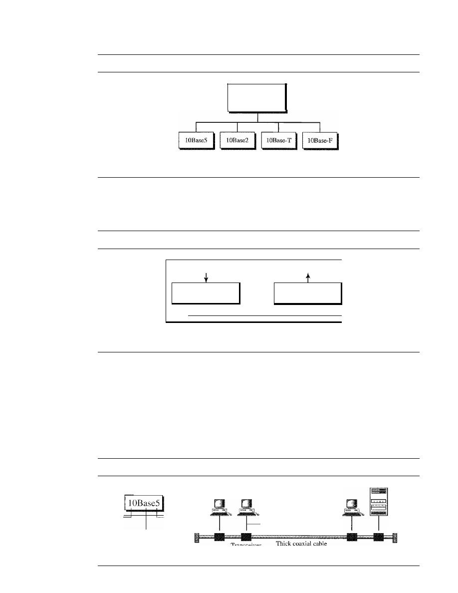
SECTION
13.2
STANDARD ETHERNET
403
Figure 13.8
Categories of Standard Ethernet
Standard Ethernet
common
implementations
Rus.
Bus,
thick coaxial
thin coaxial
Star,
UTP
Star,
fiber
Transceiver cable
maximum 50 m
received signal is interpreted as Manchester and decoded into data. As we saw in Chapter 4,
Manchester encoding is self-synchronous, providing a transition at each bit interval.
Figure 13.9 shows the encoding scheme for Standard Ethernet.
Figure 13.9
Encoding in a Standard Ethernet implementation
10 Mbps data
10 Mbps data
Manchester
Manchester
encoder
decoder
Station
I
I
I
I
I
Twisted pairs or fibers
lOBase5: Thick Ethernet
The first implementation is called
10BaseS, thick Ethernet, or Thicknet.
The nick-
name derives from the size of the cable, which is roughly the size of a garden hose
and too stiff to bend with your hands. lOBaseS was the first Ethernet specification to
use a bus topology with an external transceiver (transmitter/receiver) connected via a
tap to a thick coaxial cable. Figure 13.10 shows a schematic diagram of a lOBase5
implementation.
Figure 13.10
IOBase5 implementation
10 Mbps
500 m
Baseband
Cable
Cable
(digital)
end
end
Transceiver
T
IC
coaXial cable
maximum 500 m
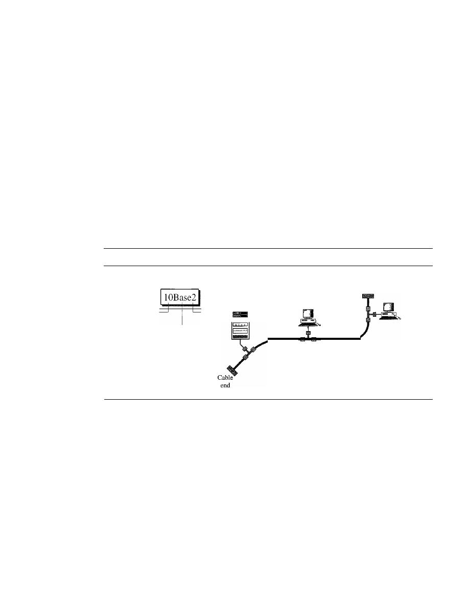
404
CHAPTER 13
WIRED LANs: ETHERNET
The transceiver is responsible for transmitting, receiving, and detecting collisions.
The
transceiver
is connected to the station via a transceiver cable that provides sepa-
rate paths for sending and receiving. This means that collision can only happen in the
coaxial cable.
The maximum length of the coaxial cable must not exceed 500 m, otherwise, there
is excessive degradation of the signal.
If
a length of more than 500 m is needed, up to
five segments, each a maximum of SOO-meter, can be connected using repeaters.
Repeaters will be discussed in Chapter 15.
10Base2: Thin Ethernet
The second implementation is called
lOBase2,
thin
Ethernet,
or
Cheapernet.
IOBase2
also uses a bus topology, but the cable is much thinner and more flexible. The cable can
be bent to pass very close to the stations. In this case, the transceiver is normally part of
the network interface card (NIC), which is installed inside the station. Figure 13.11
shows the schematic diagram of a IOBase2 implementation.
Figure 13.11
lOBase2 implementation
10 Mbps
185
m
Baseband
(digital)
Cable
end
Thin coaxial cable,
maximum 185 m
Note that the collision here occurs in the thin coaxial cable. This implementation is
more cost effective than 10BaseS because thin coaxial cable is less expensive than thick
coaxial and the tee connections are much cheaper than taps. Installation is simpler
because the thin coaxial cable is very flexible. However, the length of each segment
cannot exceed
185
m (close to 200 m) due to the high level of attenuation in thin coaxial
cable.
lOBase-T: Twisted-Pair Ethernet
The third implementation is called
lOBase-T
or
twisted-pair Ethernet. 1
OBase-T uses
a physical star topology. The stations are connected to a hub via two pairs of twisted
cable, as shown in Figure 13.12.
Note that two pairs of twisted cable create two paths (one for sending and one for
receiving) between the station and the hub. Any collision here happens in the hub.
Compared to lOBaseS or lOBase2, we can see that the hub actually replaces the coaxial
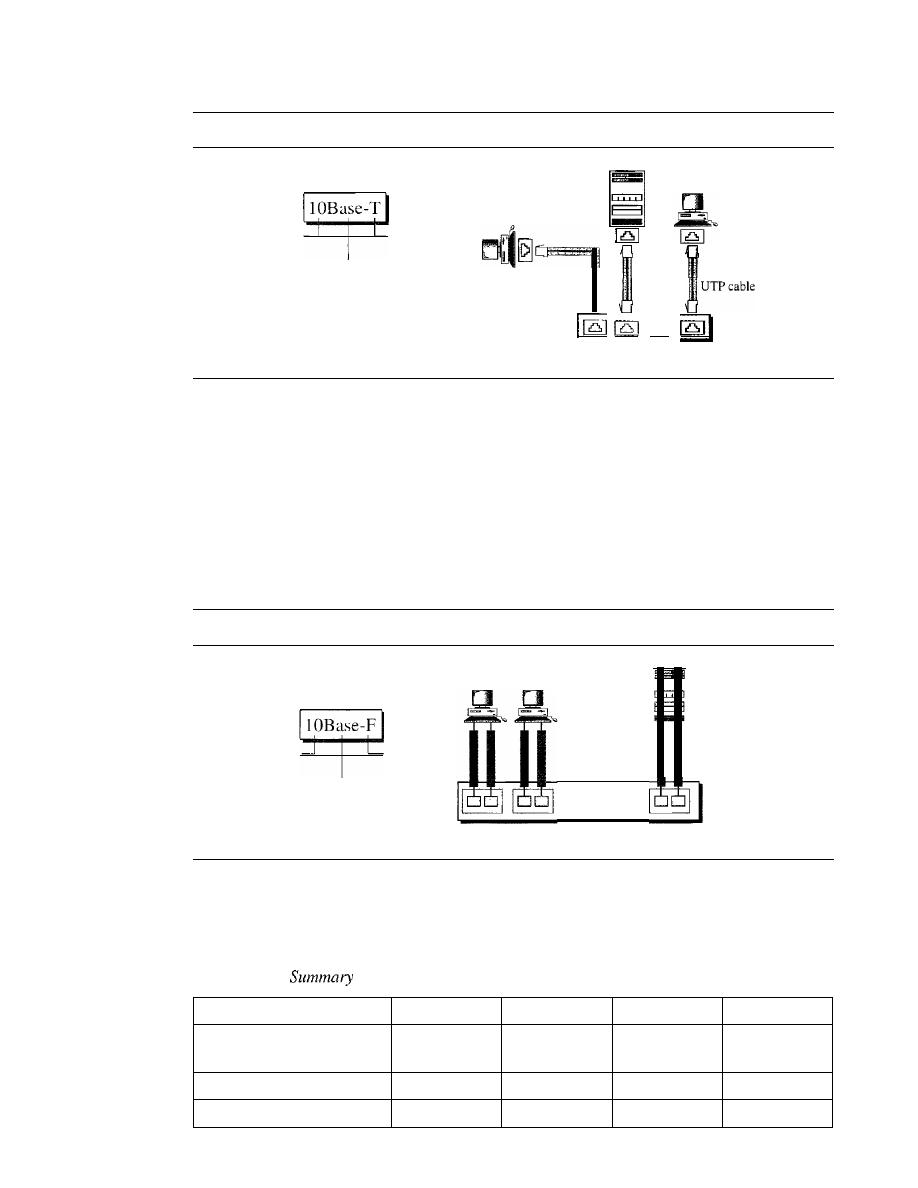
SECTION
13.2
STANDARD ETHERNET
405
Figure 13.12
IOBase-T implementation
10 Mbps
Twisted pair
Baseband
(digital)
Two pairs
of
...
lOBase-
T hub
cable as far as a collision is concerned. The maximum length of the twisted cable here
is defined as 100 m, to minimize the effect of attenuation in the twisted cable.
lOBase-F: Fiber Ethernet
Although there are several types of optical fiber lO-Mbps Ethernet, the most common is
called 10Base-F. lOBase-F uses a star topology to connect stations to a hub. The stations
are connected to the hub using two fiber-optic cables, as shown in Figure 13.13.
Figure 13.13
IOBase-F implementation
] 0
Mbps
Fiber
Baseband
(digital)
lOBase-F
hub
Two fiber-optic
cables
Summary
Table 13.1 shows a summary of Standard Ethernet implementations.
Table 13.1
of Standard Ethernet implementations
Characteristics
lOBase5
lOBase2
lOBase-T
IOBase-F
Media
Thick
Thin
2UTP
2 Fiber
coaxial cable
coaxial cable
Maximum length
500m
185 m
100m
2000m
Line encoding
Manchester
Manchester
Manchester
Manchester
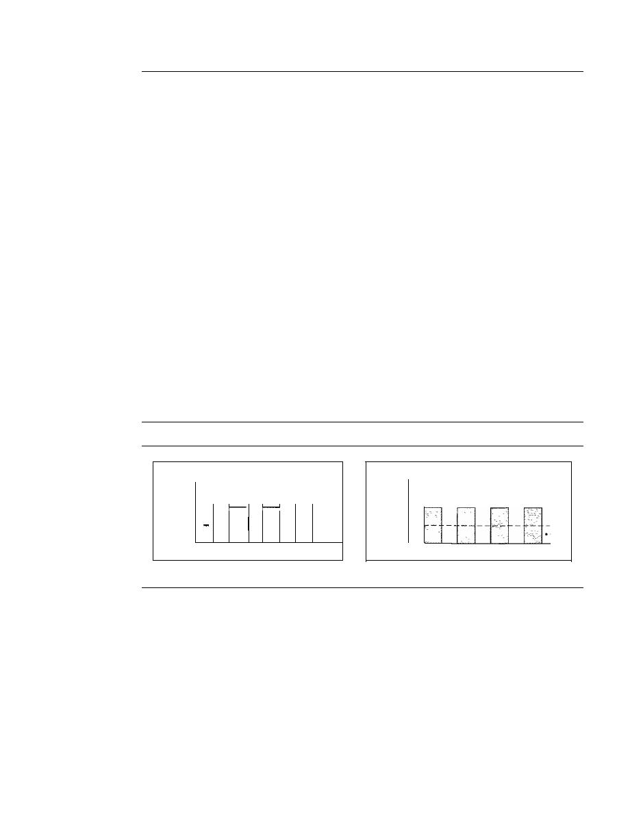
406
CHAPTER
13
WIRED LANs: ETHERNET
13.3
CHANGES IN THE STANDARD
The 10-Mbps Standard Ethernet has gone through several changes before moving to the
higher data rates. These changes actually opened the road to the evolution of the Ethernet
to become compatible with other high-data-rate LANs. We discuss some of these changes
in this section.
Bridged Ethernet
The first step in the Ethernet evolution was the division of a LAN by
bridges.
Bridges
have two effects on an Ethernet LAN: They raise the bandwidth and they separate colli-
sion domains. We discuss bridges in Chapter 15.
Raising the Bandwidth
In an unbridged Ethernet network, the total capacity (10 Mbps) is shared among all sta-
tions with a frame to send; the stations share the bandwidth of the network. If only one
station has frames to send, it benefits from the total capacity (10 Mbps). But if more
than one station needs to use the network, the capacity is shared. For example, if two
stations have a lot of frames to send, they probably alternate in usage. When one station
is sending, the other one refrains from sending. We can say that, in this case, each sta-
tion on average, sends at a rate of 5 Mbps. Figure 13.14 shows the situation.
Figure 13.14
Sharing bandwidth
Rate
One
One
One
One
frame
frame
frame
frame
10 Mbps
-
-
5 Mbps
- --
- -
--
-
- -
...
Time
Rate
10 Mbps
5 Mbps
One
One
One
One
frame
frame
frame
frame
Time
a. First station
b. Second station
The bridge, as we will learn in Chapter 15, can help here. A bridge divides the net-
work into two or more networks. Bandwidth-wise, each network is independent. For
example, in Figure 13.15, a network with 12 stations is divided into two networks, each
with 6 stations. Now each network has a capacity of 10 Mbps. The lO-Mbps capacity in
each segment is now shared between 6 stations (actually 7 because the bridge acts as a
station in each segment), not 12 stations. In a network with a heavy load, each station
theoretically is offered 10/6 Mbps instead of 10/12 Mbps, assuming that the traffic is
not going through the bridge.
It
is obvious that if we further divide the network, we can gain more bandwidth for
each segment. For example, if we use a four-port bridge, each station is now offered
10/3 Mbps, which is 4 times more than an unbridged network.
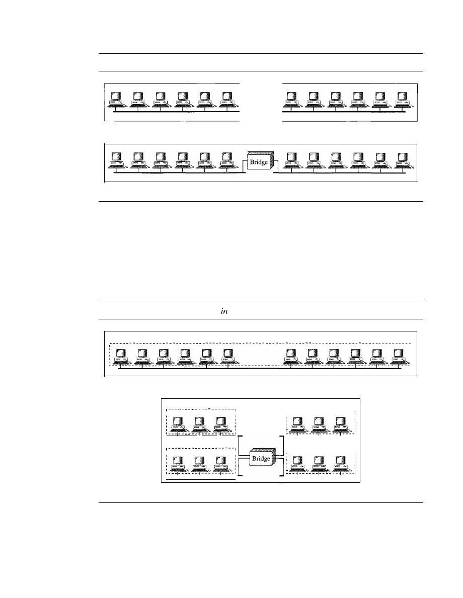
SECTION
13.3
CHANGES IN THE STANDARD
407
Figure 13.15
A network with and without a bridge
a. Without bridging
b. With bridging
Separating Collision Domains
Another advantage of a bridge is the separation of the collision domain. Figure 13.16
shows the collision domains for an unbridged and a bridged network. You can see that
the collision domain becomes much smaller and the probability of collision is reduced
tremendously. Without bridging, 12 stations contend for access to the medium; with
bridging only 3 stations contend for access to the medium.
Figure 13.16
Collision domains
an unbridged network and a bridged network
Domain
a. Without bridging
Domain
Domain
Domain
---------------------
,
,
,
,
,
,
,
1
I
I
,
,
1
Domain
,
,
,
,
,
,
b. With bridging
Switched Ethernet
The idea of a bridged LAN can be extended to a switched LAN. Instead of having two
to four networks, why not have
N
networks, where
N
is the number of stations on the
LAN? In other words, if we can have a multiple-port bridge, why not have an
N-port
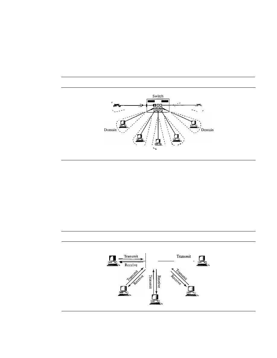
408
CHAPTER
13
WIRED IANs: ETHERNET
switch? In this way, the bandwidth is shared only between the station and the switch
(5 Mbps each). In addition, the collision domain is divided into
N
domains.
A layer 2 switch is an
N-port
bridge with additional sophistication that allows faster
handling of the packets. Evolution from a bridged Ethernet to a switched Ethernet was
a big step that opened the way to an even faster Ethernet, as we will see. Figure 13.17
shows a switched LAN.
Figure 13.17
Switched Ethernet
\
- Domain
_--
Domain
Domain--
,'-.....
\
,
Domain:
:
Domain
,
--_
I
__
Full-Duplex Ethernet
One of the limitations of 10Base5 and lOBase2 is that communication is half-duplex
(lOBase-T is always full-duplex); a station can either send or receive, but may not do both
at the same time. The next step in the evolution was to move from switched Ethernet to
full-duplex switched Ethernet. The full-duplex mode increases the capacity of each
domain from 10 to 20 Mbps. Figure 13.18 shows a switched Ethernet in full-duplex
mode. Note that instead of using one link between the station and the switch, the con-
figuration uses two links: one to transmit and one to receive.
Figure 13.18
Full-duplex switched Ethernet
Switch
II_
•
Receive
Receive
No Needfor CSMAICD
In full-duplex switched Ethernet, there is no need for the
CSMAICD
method. In a full-
duplex switched Ethernet, each station is connected to the switch via two separate links.

SECTION 13.4
FAST ETHERNET
409
Each station or switch can send and receive independently without worrying about col-
lision. Each link is a point-to-point dedicated path between the station and the switch.
There is no longer a need for carrier sensing; there is no longer a need for collision
detection. The job of the MAC layer becomes much easier. The carrier sensing and col-
lision detection functionalities of the MAC sublayer can be turned off.
MAC Control Layer
Standard Ethernet was designed as a connectionless protocol at the MAC sublayer.
There is no explicit flow control or error control to inform the sender that the frame has
arrived at the destination without error. When the receiver receives the frame, it does
not send any positive or negative acknowledgment.
To provide for flow and error control in full-duplex switched Ethernet, a new
sublayer, called the MAC control, is added between the LLC sublayer and the MAC
sublayer.
13.4
FAST ETHERNET
Fast Ethernet was designed to compete with LAN protocols such as FDDI or Fiber
Channel (or Fibre Channel, as it is sometimes spelled). IEEE created Fast Ethernet under
the name 802.3u. Fast Ethernet is backward-compatible with Standard Ethernet, but it
can transmit data 10 times faster at a rate of 100 Mbps. The goals of Fast Ethernet can be
summarized as follows:
1.
Upgrade the data rate to 100 Mbps.
2. Make it compatible with Standard Ethernet.
3. Keep the same 48-bit address.
4. Keep the same frame format.
5. Keep the same minimum and maximum frame lengths.
MAC Sublayer
A main consideration in the evolution of Ethernet from 10 to 100 Mbps was to keep the
MAC sublayer untouched. However, a decision was made to drop the bus topologies
and keep only the star topology. For the star topology, there are two choices, as we saw
before: half duplex and full duplex. In the half-duplex approach, the stations are con-
nected via a hub; in the full-duplex approach, the connection is made via a switch with
buffers at each port.
The access method is the same
(CSMAlCD)
for the half-duplex approach; for full-
duplex Fast Ethernet, there is no need for
CSMAlCD.
However, the implementations
keep
CSMA/CD
for backward compatibility with Standard Ethernet.
Autonegotiatioll
A new feature added to Fast Ethernet is called autonegotiation.
It
allows a station or a
hub a range of capabilities. Autonegotiation allows two devices to negotiate the mode
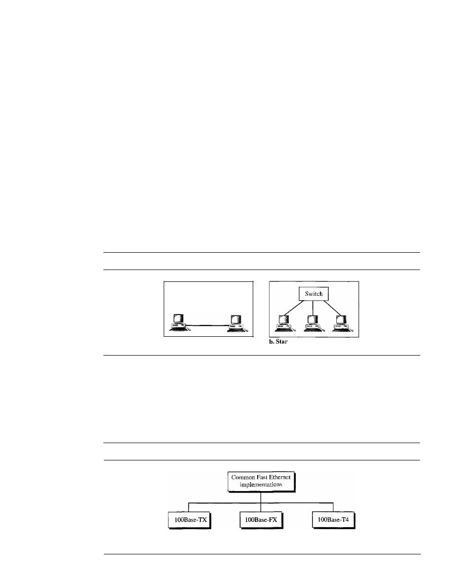
410
CHAPTER
13
WIRED LANs: ETHERNET
or data rate of operation.
It
was designed particularly for the following purposes:
o
To allow incompatible devices to connect to one another. For example, a device with
a maximum capacity of 10 Mbps can communicate with a device with a 100 Mbps
capacity (but can work at a lower rate).
o
To allow one device to have multiple capabilities.
o
To allow a station to check a hub's capabilities.
Physical Layer
The physical layer in Fast Ethernet is more complicated than the one in Standard Ethernet.
We briefly discuss some features of this layer.
Topology
Fast Ethernet is designed to connect two or more stations together.
If
there are only two
stations, they can be connected point-to-point. Three or more stations need to be con-
nected in a star topology with a hub or a switch at the center, as shown in Figure 13.19.
Figure 13.19
Fast Ethernet topology
a. Point-to-point
Implementation
Fast Ethernet implementation at the physical layer can be categorized as either two-wire
or four-wire. The two-wire implementation can be either category 5 UTP (lOOBase-TX)
or fiber-optic cable (lOOBase-FX). The four-wire implementation is designed only
for category 3 UTP (l00Base-T4). See Figure 13.20.
Figure 13.20
Fast Ethernet implementations
Two wires
category 5 UTP
Two wires
fiber
Four wires
category 3 UTP
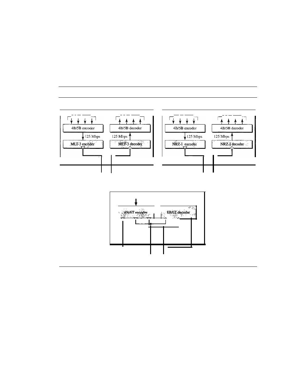
SECTION
13.4
FAST ETHERNET
411
Encoding
Manchester encoding needs a 200-Mbaud bandwidth for a data rate of 100 Mbps, which
makes it unsuitable for a medium such as twisted-pair cable. For this reason, the Fast
Ethernet designers sought some alternative encoding/decoding scheme. However,
it
was
found that one scheme would not perform equally well for all three implementations.
Therefore, three different encoding schemes were chosen (see Figure 13.21).
Figure 13.21
Encoding for Fast Ethernet implementation
100Base-TX
100Base-FX
4
x
25 Mbps
4
x
25 Mbps
4x 25 Mbps
4
x
25 Mbps
t
Station
t
Station
Two UTP category 5
Two fibers
100Base-T4
100 Mbps
100 Mbps
t
I
t
Station
1
r
-
4 category 3 UTP
lOOBase-TX
uses two pairs oftwisted-pair cable (either category 5 UTP or STP).
For this implementation, the MLT-3 scheme was selected since it has good bandwidth
performance (see Chapter 4). However, since MLT-3 is not a self-synchronous line cod-
ing scheme, 4B/5B block coding is used to provide bit synchronization by preventing
the occurrence of a long sequence of Os and Is (see Chapter 4). This creates a data rate
of 125 Mbps, which is fed into MLT-3 for encoding.
lOOBase-FX
uses two pairs of fiber-optic cables. Optical fiber can easily handle high
bandwidth requirements by using simple encoding schemes. The designers of 100Base-FX
selected the NRZ-I encoding scheme (see Chapter 4) for this implementation. However,
NRZ-I has a bit synchronization problem for long sequences of Os (or Is, based on the
encoding), as we saw in Chapter 4. To overcome this problem, the designers used 4B/5B

412
CHAPTER
13
WIRED LANs: ETHERNET
block encoding as we described for IOOBase-TX. The block encoding increases the bit rate
from 100 to 125 Mbps, which can easily be handled by fiber-optic cable.
A 1OOBase-TX network can provide a data rate of 100 Mbps, but it requires the use of
category 5 UTP or STP cable. This is not cost-efficient for buildings that have already been
wired for voice-grade twisted-pair (category 3). A new standard, called
lOOBase-T4, was
designed to use category 3 or higher UTP. The implementation uses four pairs of UTP for
transmitting 100 Mbps. Encoding/decoding in 100Base-T4 is more complicated. As this
implementation uses category 3 UTP, each twisted-pair cannot easily handle more than
25 Mbaud. In this design, one pair switches between sending and receiving. Three pairs of
UTP category 3, however, can handle only 75 Mbaud (25 Mbaud) each. We need to use an
encoding scheme that converts 100 Mbps to a 75 Mbaud signal. As we saw in Chapter 4,
8B/6T satisfies this requirement. In 8B/6T, eight data elements are encoded as six signal
elements. This means that 100 Mbps uses only (6/8)
x
100 Mbps, or 75 Mbaud.
Summary
Table 13.2 is a summary of the Fast Ethernet implementations.
Table 13.2
Summary of Fast Ethernet implementations
Characteristics
lOOBase-TX
lOOBase-FX
100Base-T4
Media
Cat 5 UTP or STP
Fiber
Cat 4 UTP
Number of wires
2
2
4
Maximum length
100m
100m
100m
Block encoding
4B/5B
4B/5B
Line encoding
MLT-3
NRZ-I
8B/6T
13.5
GIGABIT ETHERNET
The need for an even higher data rate resulted in the design of the Gigabit Ethernet
protocol (1000 Mbps). The IEEE committee calls the Standard 802.3z. The goals of the
Gigabit Ethernet design can be summarized as follows:
1. Upgrade the data rate to 1 Gbps.
2. Make it compatible with Standard or Fast Ethernet.
3. Use the same 48-bit address.
4. Use the same frame format.
5. Keep the same minimum and maximum frame lengths.
6. To support autonegotiation as defined in Fast Ethernet.
MAC Sublayer
A main consideration in the evolution of Ethernet was to keep the MAC sublayer
untouched. However, to achieve a data rate 1 Gbps, this was no longer possible. Gigabit
Ethernet has two distinctive approaches for medium access: half-duplex and full-duplex.

SECTION
13.5
GIGABIT ETHERNET
413
Almost all implementations of Gigabit Ethernet follow the full-duplex approach. How-
ever, we briefly discuss the half-duplex approach to show that Gigabit Ethernet can be
compatible with the previous generations.
Full-Duplex Mode
In full-duplex mode, there is a central switch connected to all computers or other
switches. In this mode, each switch has buffers for each input port in which data are
stored until they are transmitted. There is no collision in this mode, as we discussed
before. This means that CSMAlCD is not used. Lack of collision implies that the max-
imum length of the cable is determined by the signal attenuation in the cable, not by the
collision detection process.
In the full-duplex mode of Gigabit Ethernet, there is no collision;
the maximum length of the cable
is
determined by the signal attenuation in the cable.
Half-Duplex Mode
Gigabit Ethernet can also be used in half-duplex mode, although it is rare. In this case,
a switch can be replaced by a hub, which acts as the common cable in which a collision
might occur. The half-duplex approach uses CSMAlCD. However, as we saw before,
the maximum length of the network in this approach is totally dependent on the minimum
frame size. Three methods have been defined: traditional, carrier extension, and frame
bursting.
Traditional
In the traditional approach, we keep the minimum length of the frame as
in traditional Ethernet (512 bits). However, because the length of a bit is 11100 shorter
in Gigabit Ethernet than in lO-Mbps Ethernet, the slot time for Gigabit Ethernet is
512 bits x 111000
JlS,
which is equal to 0.512
JlS.
The reduced slot time means that colli-
sion is detected 100 times earlier. This means that the maximum length of the network is
25 m. This length may be suitable if all the stations are in one room, but it may not even
be long enough to connect the computers in one single office.
Carrier Extension
To allow for a longer network, we increase the minimum frame
length. The carrier extension approach defines the minimum length of a frame as 512 bytes
(4096 bits). This means that the minimum length is 8 times longer. This method forces
a station to add extension bits (padding) to any frame that is less than 4096 bits. In this
way, the maximum length of the network can be increased 8 times to a length of 200 m.
This allows a length of 100 m from the hub to the station.
Frame Bursting
Carrier extension is very inefficient if we have a series of short
frames to send; each frame carries redundant data. To improve efficiency, frame bursting
was proposed. Instead of adding an extension to each frame, multiple frames are sent.
However, to make these multiple frames look like one frame, padding is added between
the frames (the same as that used for the carrier extension method) so that the channel
is not idle. In other words, the method deceives other stations into thinking that a very
large frame has been transmitted.
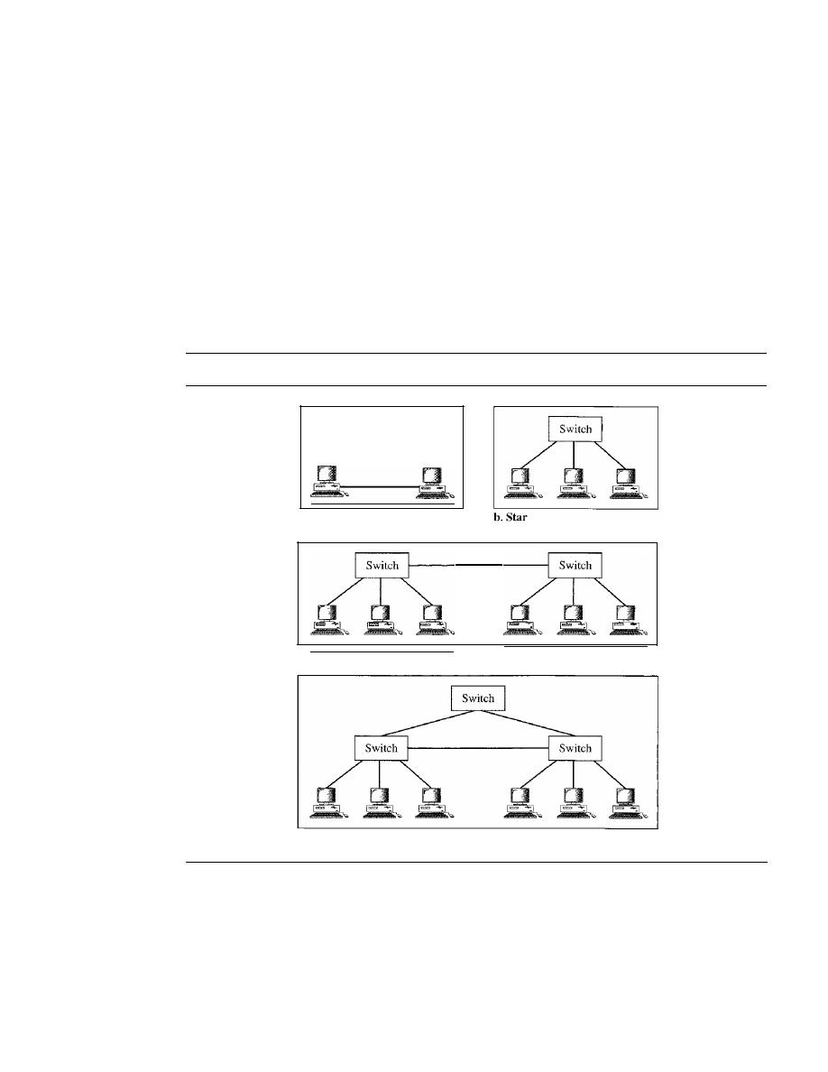
414
CHAPTER
13
WIRED LANs: ETHERNET
Physical Layer
The physical layer in Gigabit Ethernet is more complicated than that in Standard or Fast
Ethernet. We briefly discuss some features of this layer.
Topology
Gigabit Ethernet is designed to connect two or more stations.
If
there are only two sta-
tions, they can be connected point-to-point. Three or more stations need to be connected
in a star topology with a hub or a switch at the center. Another possible configuration is
to connect several star topologies or let a star topology be part of another as shown in
Figure 13.22.
Figure 13.22
Topologies of Gigabit Ethernet
a. Point-to-point
c. Two stars
d. Hierarchy of stars
Implementation
Gigabit Ethernet can be categorized as either a two-wire or a four-wire implementation.
The two-wire implementations use fiber-optic cable
(1000Base-SX, short-wave,
or
lOOOBase-LX, long-wave),
or STP
(1000Base-CX).
The four-wire version uses cate-
gory 5 twisted-pair cable
(lOOOBase-
T). In other words, we have four implementations,
as shown in Figure 13.23. lOOOBase-T was designed in response to those users who
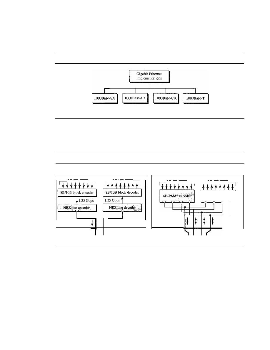
SECTION 13.5
GIGABIT ETHERNET
415
had already installed this wiring for other purposes such as Fast Ethernet or telephone
serVIces.
Figure 13.23
Gigabit Ethernet implementations
Two-wire
Two-wire
Two-wire
short-wave tiber
long-wave tiber
copper (STP)
Four-wire
UTP
Encoding
Figure 13.24 shows the encoding/decoding schemes for the four implementations.
Figure 13.24
Encoding in Gigabit Ethernet implementations
IOOOBase-SX. lOOOBase-LX, and IOOOBase-CX
IOOOBase-T
4D-PAM5 decoder
8
x
125 Mbps
8
x
125 Mbps
Station
t
8
x
125 Mbps
8
x
125 Mbps
Station
Two fibers or two
STPs
4 UTPcables
Gigabit Ethernet cannot use the Manchester encoding scheme because it involves a
very high bandwidth (2 GBaud). The two-wire implementations use an NRZ scheme, but
NRZ does not self-synchronize properly. To synchronize bits, particularly at this high
data rate, 8BIl OB block encoding, discussed in Chapter 4, is used.
This block encoding prevents long sequences of Os or Is in the stream, but the result-
ing stream is 1.25 Gbps. Note that in this implementation, one wire (fiber or STP) is
used for sending and one for receiving.
In the four-wire implementation it is not possible to have 2 wires for input and 2 for
output, because each wire would need to carry 500 Mbps, which exceeds the capacity
for category 5 UTP. As a solution, 4D-PAM5 encoding, as discussed in Chapter 4, is used
to reduce the bandwidth. Thus, all four wires are involved in both input and output; each
wire carries 250 Mbps, which is in the range for category 5 UTP cable_
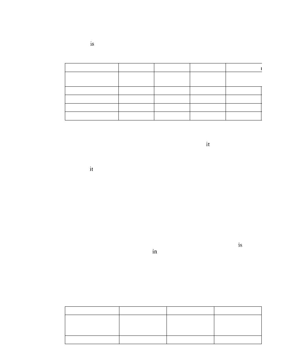
416
CHAPTER
13
WIRED IANs: ETHERNET
Summary
Table 13.3
a summary of the Gigabit Ethernet implementations.
Table 13.3
Summary of Gigabit Ethernet implementations
Characteristics
lOOOBase-SX
lOOOBase-LX
lOOOBase-CX
lOOOBase-T
Media
Fiber
Fiber
STP
Cat 5 UTP
I
I
short-wave
long-wave
Number of wires
2
2
2
4
Maximum length
550m
5000m
25m
100m
Block encoding
8B/lOB
8B/lOB
8B/lOB
Line encoding
NRZ
NRZ
NRZ
4D-PAM5
Ten-Gigabit Ethernet
The IEEE committee created Ten-Gigabit Ethernet and called
Standard 802.3ae. The
goals of the Ten-Gigabit Ethernet design can be summarized as follows:
1. Upgrade the data rate to 10 Gbps.
2. Make
compatible with Standard, Fast, and Gigabit Ethernet.
3. Use the same 48-bit address.
4. Use the same frame format.
S.
Keep the same minimum and maximum frame lengths.
6. Allow the interconnection of existing LANs into a metropolitan area network (MAN)
or a wide area network (WAN).
7. Make Ethernet compatible with technologies such as Frame Relay and ATM (see
Chapter 18).
MAC Sublayer
Ten-Gigabit Ethernet operates only in full duplex mode which means there
no need
for contention;
CSMA/CD
is not used
Ten-Gigabit Ethernet.
Physical Layer
The physical layer in Ten-Gigabit Ethernet is designed for using fiber-optic cable over long
distances. Three implementations are the most common: lOGBase-S, lOGBase-L, and
lOGBase-E. Table 13.4 shows a summary of the Ten-Gigabit Ethernet implementaions.
Table 13.4
Summary ofTen-Gigabit Ethernet implementations
Characteristics
lOGBase-S
lOGBase-L
lOGBase-E
Media
Short-wave
Long-wave
Extended
S50-nrn
131O-nrn
1550-mrn
rnultimode
single mode
single mode
Maximum length
300m
lOkm
40km

SECTION
13.8
SUMMARY
417
13.6
RECOMMENDED READING
For more details about subjects discussed in this chapter, we recommend the following
books. The items in brackets [...] refer to the reference list at the end of the text.
Books
Ethernet is discussed in Chapters 10, 11, and 12 of [For03], Chapter 5 of [Kei02], Sec-
tion 4.3 of [Tan03], and Chapters 15 and 16 of [Sta04]. [SpuOO] is a book about Ethernet.
A complete discussion of Gigabit Ethernet can be found in [KCK98] and [Sau98].
Chapter 2 of [IzzOO] has a good comparison between different generations of Ethernet.
13.7
KEY TERMS
1000Base-CX
1000Base-LX
1000Base-SX
1000Base-T
100Base-FX
100Base-T4
100Base-TX
10Base2
lOBase5
lOBase-F
10Base-T
10GBase-E
lOGBase-L
10GBase-S
autonegotiation
bridge
carrier extension
Cheapernet
collision domain
destination service access point (DSAP)
Fast Ethernet
frame bursting
full-duplex switched Ethernet
Gigabit Ethernet
hexadecimal notation
logical
link control (LLC)
media access control (MAC)
network interface card (NIC)
preamble
Project 802
source service access point (SSAP)
Standard Ethernet
switch
switched Ethernet
Ten-Gigabit Ethernet
thick Ethernet
Thicknet
thin Ethernet
transceiver
twisted-pair Ethernet
13.8
SUMMARY
o
Ethernet is the most widely used local area network protocoL
o
The IEEE 802.3 Standard defines I-persistent
CSMA/CD
as the access method for
first-generation 10-Mbps Ethernet.
o
The data link layer of Ethernet consists of the LLC sublayer and the MAC sublayer.

418
CHAPTER
13
WIRED
ETHERNET
o
The MAC sublayer is responsible for the operation of the
CSMAlCD
access
method and framing.
o
Each station on an Ethernet network has a unique 48-bit address imprinted on its
network interface card (NIC).
o
The minimum frame length for lO-Mbps Ethernet is 64 bytes; the maximum is
1518 bytes.
o
The common implementations of lO-Mbps Ethernet are lOBase5 (thick Ethernet),
10Base2 (thin Ethernet),
(twisted-pair Ethernet), and lOBase-F (fiber
Ethernet).
o
The 10Base5 implementation of Ethernet uses thick coaxial cable. lOBase2 uses
thin coaxial cable. lOBase-T uses four twisted-pair cables that connect each station
to a common hub. lOBase-F uses fiber-optic cable.
o
A bridge can increase the bandwidth and separate the collision domains on an
Ethernet LAN.
o
A switch allows each station on an Ethernet LAN to have the entire capacity of the
network to itself.
o
Full-duplex mode doubles the capacity of each domain and removes the need for
the
CSMAlCD
method.
o
Fast Ethernet has a data rate of 100 Mbps.
o
In
Fast Ethernet, autonegotiation allows two devices to negotiate the mode or data
rate of operation.
o
The common Fast Ethernet implementations are 1OOBase-TX (two pairs of twisted-
pair cable), lOOBase-FX (two fiber-optic cables), and 100Base-T4 (four pairs of
voice-grade, or higher, twisted-pair cable).
o
Gigabit Ethernet has a data rate of 1000 Mbps.
o
Gigabit Ethernet access methods include half-duplex mode using traditional
CSMAI
CD (not common) and full-duplex mode (most popular method).
o
The common Gigabit Ethernet implementations are 1000Base-SX (two optical fibers
and a short-wave laser source), 1000Base-LX (two optical fibers and a long-wave
laser source), and 1000Base-T (four twisted pairs).
o
The latest Ethernet standard is Ten-Gigabit Ethernet that operates at 10 Gbps. The
three common implementations are lOGBase-S, 10GBase-L, and 10GBase-E. These
implementations use fiber-optic cables in full-duplex mode.
13.9
PRACTICE SET
Review Questions
1.
How is the preamble field different from the SFD field?
2. What is the purpose of an NIC?
3. What is the difference between a unicast, multicast, and broadcast address?
4. What are the advantages of dividing an Ethernet LAN with a bridge?
5. What is the relationship between a switch and a bridge?

SECTION
13.9
PRACTICE SET
419
6. Why is there no need for
CSMAlCD
on a full-duplex Ethernet LAN?
7. Compare the data rates for Standard Ethernet, Fast Ethernet, Gigabit Ethernet, and
Ten-Gigabit Ethernet.
8. What are the common Standard Ethernet implementations?
9. What are the common Fast Ethernet implementations?
10. What are the common Gigabit Ethernet implementations?
11. What are the common Ten-Gigabit Ethernet implementations?
Exercises
12. What is the hexadecimal equivalent of the following Ethernet address?
01011010 00010001 01010101 00011000 10101010 00001111
13. How does the Ethernet address lA:2B:3CAD:5E:6F appear on the line in binary?
14.
If
an Ethernet destination address is 07:01:02:03:04:05, what is the type of the
address (unicast, multicast, or broadcast)?
15. The address 43:7B:6C:DE: 10:00 has been shown as the source address in an Ethernet
frame. The receiver has discarded the frame. Why?
16. An Ethernet MAC sublayer receives 42 bytes of data from the upper layer. How
many bytes of padding must be added to the data?
17. An Ethernet MAC sublayer receives 1510 bytes of data from the upper layer. Can
the data be encapsulated in one frame?
If
not, how many frames need to be sent?
What is the size of the data in each frame?
18. What is the ratio of useful data to the entire packet for the smallest Ethernet frame?
What is the ratio for the largest frame?
19. Suppose the length of a lOB ase5 cable is 2500 m.
If
the speed of propagation in a
thick coaxial cable is 200,000,000 m!s, how long does it take for a bit to travel
from the beginning to the end of the network? Assume there are 10
delay in the
equipment.
20. The data rate of lOBase5 is 10 Mbps. How long does it take to create the smallest
frame? Show your calculation.


CHAPTER 14
Wireless LANs
Wireless communication is one of the fastest-growing technologies. The demand for
connecting devices without the use of cables is increasing everywhere. Wireless LANs
can be found on college campuses, in office buildings, and in many public areas.
In this chapter, we concentrate on two promising wireless technologies for LANs:
IEEE 802.11 wireless LANs, sometimes called wireless Ethernet, and Bluetooth, a
technology for small wireless LANs. Although both protocols need several layers to
operate, we concentrate mostly on the physical and data link layers.
14.1
IEEE 802.11
IEEE has defined the specifications for a wireless LAN, called IEEE
802.11,
which
covers the physical and data link layers.
Architecture
The standard defines two kinds of services: the basic service set (BSS) and the extended
service set (ESS).
Basic Service Set
IEEE 802.11 defines the basic service set (BSS) as the building block of a wireless
LAN. A basic service set is made of stationary or mobile wireless stations and an optional
central base station, known as the access point (AP). Figure 14.1 shows two sets in this
standard.
The BSS without anAP is a stand-alone network and cannot send data to other BSSs.
It
is called an
ad hoc architecture. In this architecture, stations can form a network
without the need of an AP; they can locate one another and agree to be part of a BSS. A
BSS with an AP is sometimes referred to as an
infrastructure network.
A BSS without an AP is called an ad hoc network;
a BSS with an AP is called an infrastructure network.
421
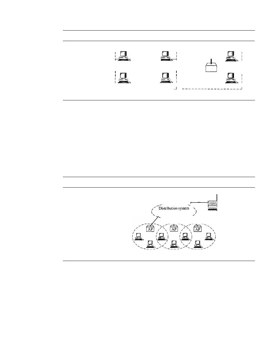
422
CHAPTER
14
WIRELESS LANs
Figure 14.1
Basic service sets (BSSs)
AP
Station
-------------------
1
Station
:
I
I
Station
Station
I
Infrastructure (BSS with an AP)
1---------- ------ ---I
1
•
•
1
1
Station
Station
1
I
I
I
I
I
Station
Station
1
l
Ad hoc network (SSS without an
AP)
BSS: Basic service set
AP: Access point
Extended Service Set
An
extended service set (ESS)
is made up of two or more BSSs with APs. In this
case, the BSSs are connected through a distribution system, which is usually a wired
LAN. The distribution system connects the APs in the BSSs. IEEE 802.11 does not
restrict the distribution system; it can be any IEEE LAN such as an Ethernet. Note that
the extended service set uses two types of stations: mobile and stationary. The mobile
stations are normal stations inside a BSS. The stationary stations are AP stations that
are part of a wired LAN. Figure 14.2 shows an ESS.
Figure 14.2
Extended service sets (ESSs)
--------
ESS: Extended service set
BSS: Basic service set
AP:
Access point
Server or
Gateway
BSS
BSS
BSS
When BSSs are connected, the stations within reach of one another can communi-
cate without the use of an AP. However, communication between two stations in two
different BSSs usually occurs via two APs. The idea is similar to communication in a
cellular network if we consider each BSS to be a cell and each AP to be a base station.
Note that a mobile station can belong to more than one BSS at the same time.
Station Types
IEEE 802.11 defines three types of stations based on their mobility in a wireless LAN:
no-transition, BSS·transition,
and
ESS-transition mobility.
A station with no-transition
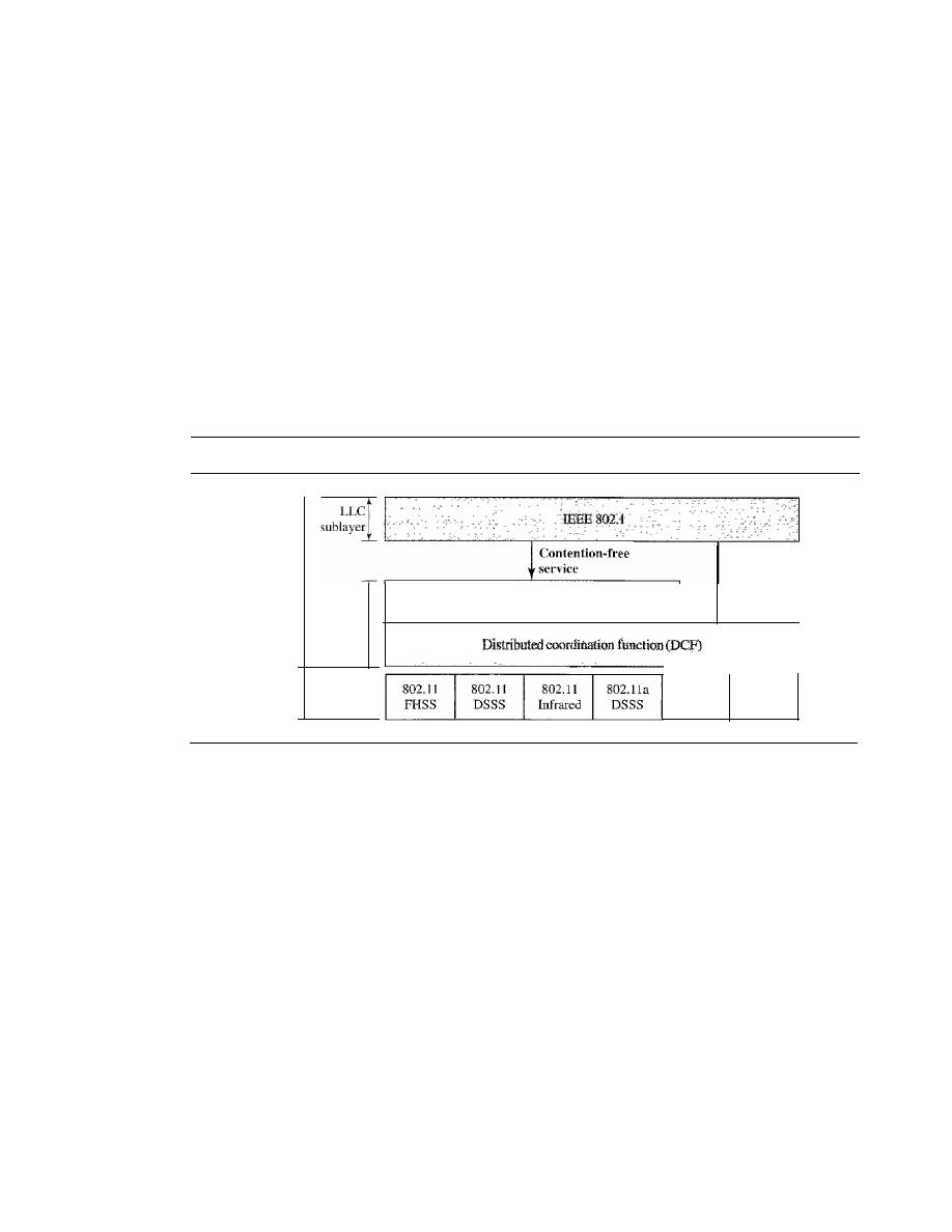
SECTION 14.1
IEEE 802.11
423
mobility is either stationary (not moving) or moving only inside a BSS. A station with
BSS-transition mobility can move from one BSS to another, but the movement is con-
fined inside one ESS. A station with ESS-transition mobility can move from one ESS to
another. However, IEEE 802.11 does not guarantee that communication is continuous
during the move.
MAC Sublayer
IEEE 802.11 defines two MAC sublayers: the distributed coordination function (DCF)
and point coordination function (PCF). Figure
14.3
shows the relationship between the
two MAC sublayers, the LLC sublayer, and the physical layer. We discuss the physical
layer implementations later in the chapter and will now concentrate on the MAC
sublayer.
Figure 14.3
MAC layers in IEEE 802.11 standard
Data link
layer
MAC
sublayer
Point coordination function (PCF)
Contention
service
Physical
layer
802.Ila
802.l1g
OFDM
DSSS
Distributed Coordination Function
One of the two protocols defined by IEEE at the MAC sublayer is called the distributed
coordination function (DCF). DCF uses
CSMAICA
(as defined in Chapter 12) as the
access method. Wireless LANs cannot implement
CSMAfCD
for three reasons:
I.
For collision detection a station must be able to send data and receive collision
signals at the same time. This can mean costly stations and increased bandwidth
requirements.
2. Collision may not be detected because of the hidden station problem. We will discuss
this problem later in the chapter.
3. The distance between stations can be great. Signal fading could prevent a station at
one end from hearing a collision at the other end.
Process Flowchart
Figure
14.4
shows the process flowchart for
CSMAICA
as used
in wireless LANs. We will explain the steps shortly.
Frame Exchange Time Line
Figure
14.5
shows the exchange of data and control
frames in time.
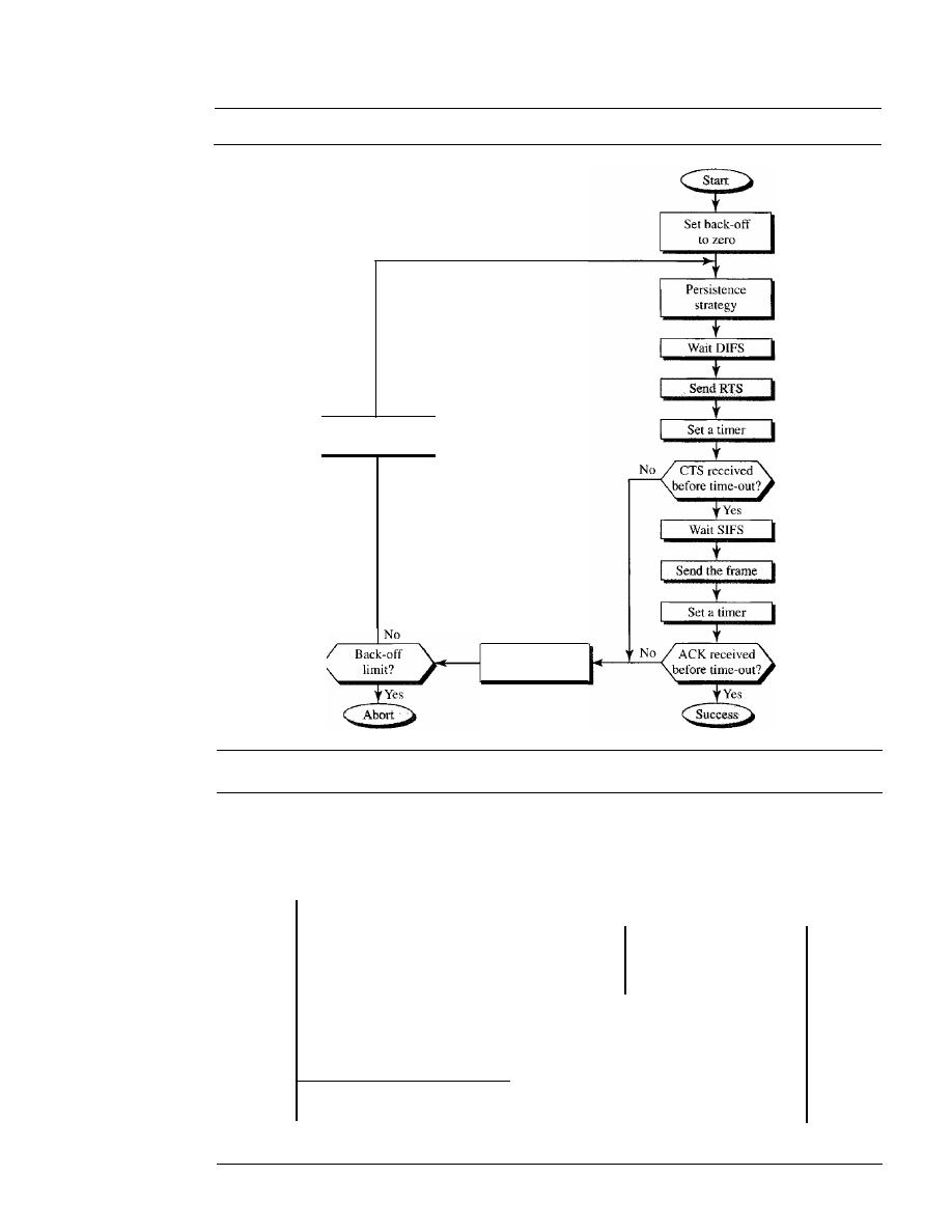
424
CHAPTER
14
WIRELESS LANs
Figure 14.4
CSMAICA flowchart
Wait back-off
time
Time
Increment
back-off
Time
Time
Time

SECTION 14.1
IEEE 802.11
425
I.
Before sending a frame, the source station senses the medium by checking the
energy level at the carrier frequency.
a. The channel uses a persistence strategy with back-off until the channel is idle.
b. After the station is found to be idle, the station waits for a period of time called
the distributed interframe space (DIFS); then the station sends a control
frame called the request to send (RTS).
2. After receiving the RTS and waiting a period of time called the short interframe
space (SIFS), the destination station sends a control frame, called the clear to
send (CTS), to the source station. This control frame indicates that the destination
station is ready to receive data.
3. The source station sends data after waiting an amount of time equal to SIFS.
4. The destination station, after waiting an amount of time equal to SIFS, sends an
acknowledgment to show that the frame has been received. Acknowledgment is
needed in this protocol because the station does not have any means to check for
the successful arrival of its data at the destination. On the other hand, the lack of
collision in
CSMAlCD
is a kind of indication to the source that data have arrived.
Network Allocation Vector
How do other stations defer sending their data if one
station acquires access? In other words, how is the collision avoidance aspect of this
protocol accomplished? The key is a feature called NA
V.
When a station sends an RTS frame, it includes the duration of time that it needs to
occupy the channel. The stations that are affected by this transmission create a timer
called a network allocation vector (NAV) that shows how much time must pass before
these stations are allowed to check the channel for idleness. Each time a station
accesses the system and sends an RTS frame, other stations start their NA
V.
In other
words, each station, before sensing the physical medium to see if it is idle, first checks
its NAV to see if it has expired. Figure 14.5 shows the idea of NA
V.
Collision During Handshaking
What happens if there is collision during the time
when RTS or CTS control frames are in transition, often called the handshaking period?
Two or more stations may try to send RTS frames at the same time. These control frames
may collide. However, because there is no mechanism for collision detection, the sender
assumes there has been a collision if it has not received a CTS frame from the receiver.
The back-off strategy is employed, and the sender tries again.
Point Coordination Function (PCP)
The point coordination function (PCF) is an optional access method that can be imple-
mented in an infrastructure network (not in an ad hoc network).
It
is implemented on top
of the DCF and is used mostly for time-sensitive transmission.
PCF has a centralized, contention-free polling access method. The AP performs
polling for stations that are capable of being polled. The stations are polled one after
another, sending any data they have to the AP.
To give priority to PCF over DCF, another set of interframe spaces has been
defined: PIFS and SIFS. The SIFS is the same as that in DCF, but the PIFS (PCF IFS) is
shorter than the DIFS. This means that if, at the same time, a station wants to use only
DCF and an AP wants to use PCF, the AP has priority.
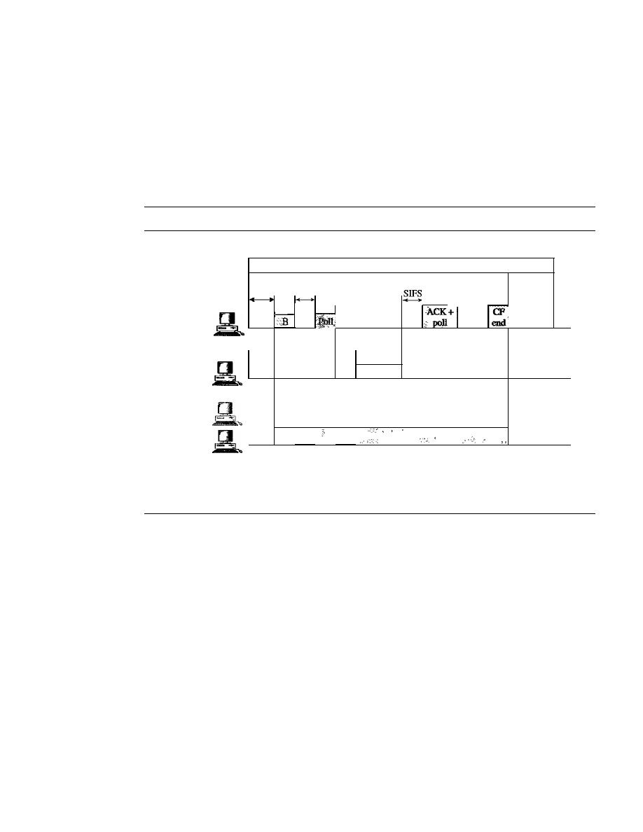
426
CHAPTER
14
WIRELESS LANs
Due to the priority of PCF over DCF, stations that only use DCF may not gain
access to the medium. To prevent this, a repetition interval has been designed to cover
both contention-free (PCF) and contention-based (DCF) traffic. The
repetition interval,
which is repeated continuously, starts with a special control frame, called a beacon frame.
When the stations hear the beacon frame, they start their NAV for the duration of the
contention-free period of the repetition interval. Figure 14.6 shows an example of a rep-
etition interval.
Figure 14.6
Example of repetition interval
B: Beacon frame
CF: Contention-free
AP
Polled
station
Others
..
Repetition interval
Contention-free
Contention
PIFS
SIFS
poll
• ••
end
Time
SIFS
--
ACK
+
data
Time
NAV
Time
During the repetition interval, the PC (point controller) can send a poll frame,
receive data, send an ACK, receive an ACK, or do any combination of these (802.11
uses piggybacking). At the end of the contention-free period, the PC sends a CF end
(contention-free end) frame to allow the contention-based stations to use the medium.
Fragmentation
The wireless environment is very noisy; a corrupt frame has to be retransmitted. The
protocol, therefore, recommends fragmentation-the division of a large frame into
smaller ones. It is more efficient to resend a small frame than a large one.
Frame Format
The MAC layer frame consists of nine fields, as shown in Figure 14.7.
o
Frame control
(Fe).
The FC field is 2 bytes long and defines the type of frame and
some control information. Table 14.1 describes the subfields. We will discuss each
frame type later in this chapter.
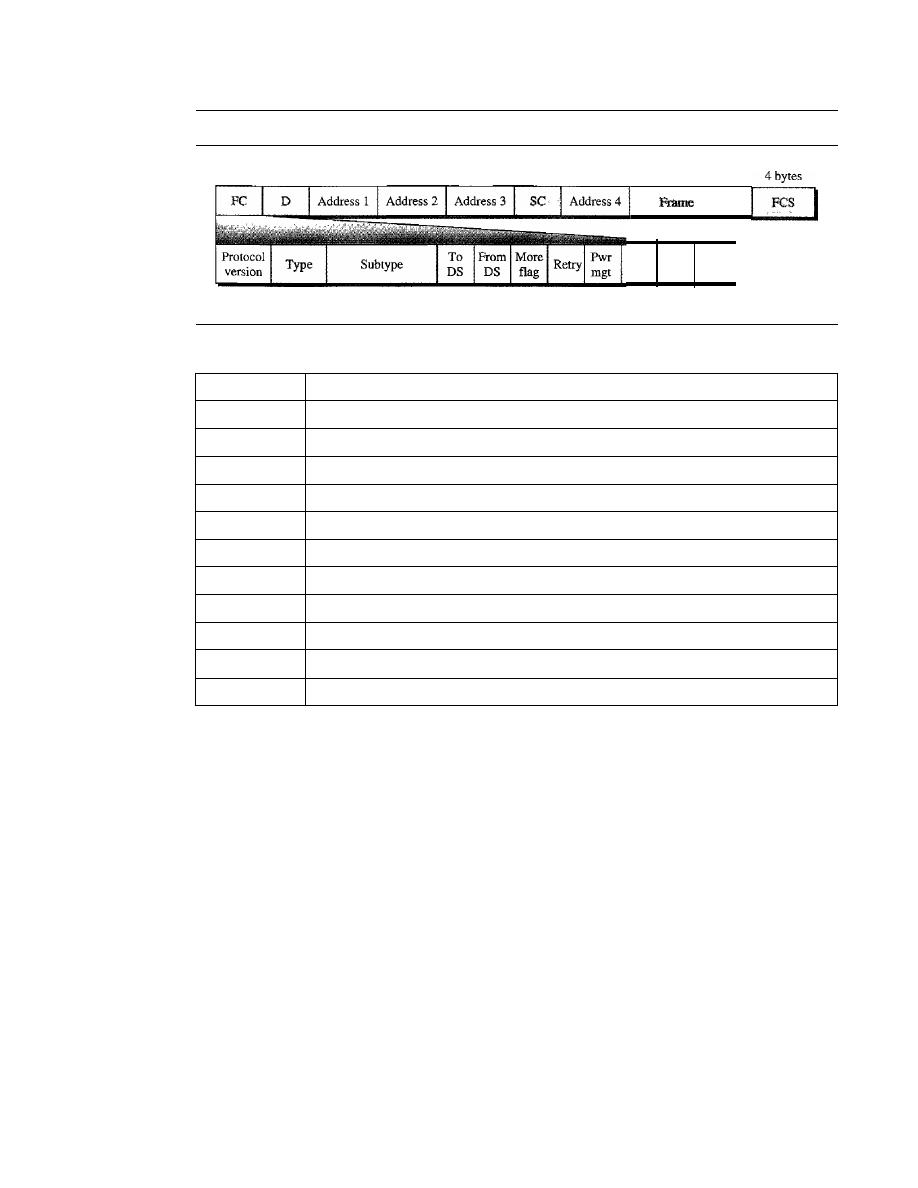
SECTION
14.1
IEEE 802.11
427
Figure 14.7
Frameformat
2 bytes 2 bytes
6 bytes
6
bytes
6 bytes
2 bytes
6 bytes
o
to
2312
bytes
body
More WEP Rsvd
data
2 bits
2
bits
4 bits
1 bit
1 bit
1 bit
1 bit
1 bit
1 bit
1 bit
1 bit
Table 14.1
Subfields in FC field
Field
Explanation
Version
Current version is 0
Type
Type of information: management (00), control (01), or data (10)
Subtype
Subtype of each type (see Table 14.2)
ToDS
Defined later
FromDS
Defined later
More flag
When set to 1, means more fragments
Retry
When set to 1, means retransmitted frame
Pwr mgt
When set to 1, means station is in power management mode
More data
When set to 1, means station has more data to send
WEP
Wired equivalent privacy (encryption implemented)
Rsvd
Reserved
D
D. In all frame types except one, this field defines the duration of the transmission
that is used to set the value of NAY. In one control frame, this field defines the ID
of the frame.
D
Addresses. There are four address fields, each 6 bytes long. The meaning of each
address field depends on the value of the
To
DS and
From
DS subfields and will
be
discussed later.
D
Sequence control. This field defines the sequence number of the frame to be used
in flow control.
D
Frame body. This field, which can be between 0 and 2312 bytes, contains infor-
mation based on the type and the subtype defined in the FC field.
D
FCS. The FCS field is 4 bytes long and contains a CRC-32 error detection sequence.
Frame Types
A wireless LAN defined by IEEE 802.11 has three categories of frames: management
frames, control frames, and data frames.
Management Frames
Management frames are used for the initial communication
between stations and access points.
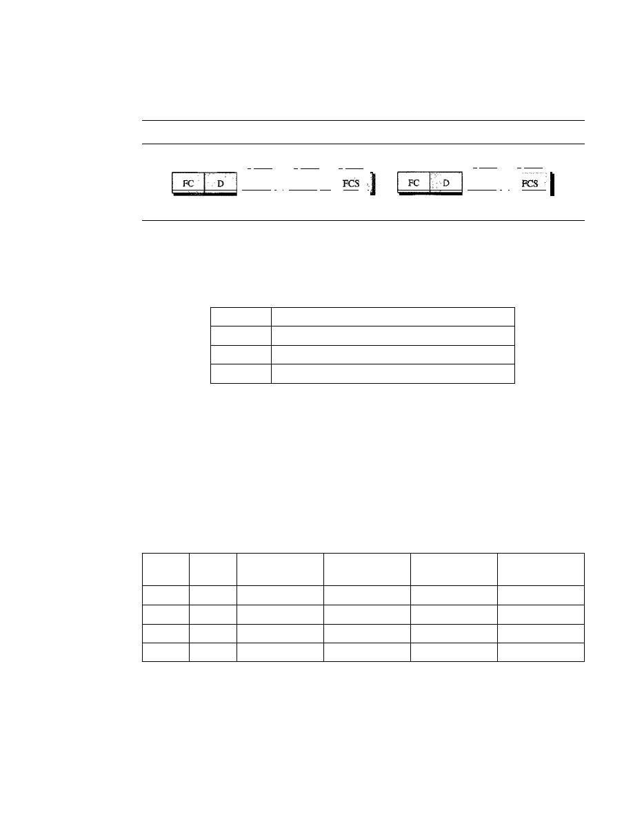
428
CHAPTER
14
WIRELESS LANs
Control Frames
Control frames are used for accessing the channel and acknowledg-
ing frames. Figure 14.8 shows the format.
Figure
14.8
Controlframes
2 bytes 2 bytes
6 bytes
6 bytes
4 bytes
Address 1
I
Address
21
RTS
2 bytes 2 bytes
6 bytes
4 bytes
Address 1
I
CTSor ACK
For control frames the value of the type field is 0 I; the values of the subtype fields
for frames we have discussed are shown in Table 14.2.
Table
14.2
Values of subfields in control frames
Subtype
Meaning
1011
Request to send (RTS)
1100
Clear to send (CTS)
1101
Acknowledgment (ACK)
Data Frames
Data frames are used for carrying data and control information.
Addressing Mechanism
The IEEE 802.11 addressing mechanism specifies four cases, defined by the value of the
two flags in the FC field, To DS and From DS. Each flag can be either 0 or I, resulting in
four different situations. The interpretation of the four addresses (address I to address 4)
in the MAC frame depends on the value of these flags, as shown in Table 14.3.
Table
14.3
Addresses
To
From
Address
Address
Address
Address
DS
DS
1
2
3
4
0
0
Destination
Source
BSS ID
N/A
0
1
Destination
SendingAP
Source
N/A
1
0
Receiving AP
Source
Destination
N/A
1
1
Receiving AP
SendingAP
Destination
Source
Note that address 1 is always the address of the next device. Address 2 is always
the address of the previous device. Address 3 is the address of the final destination sta-
tion if it is not defined by address I. Address 4 is the address of the original source
station if it is not the same as address 2.
o
Case 1: 00 In this case, To DS
=
0 and From DS
=
O. This means that the frame is
not going to a distribution system (To DS
=
0) and is not coming from a distribution
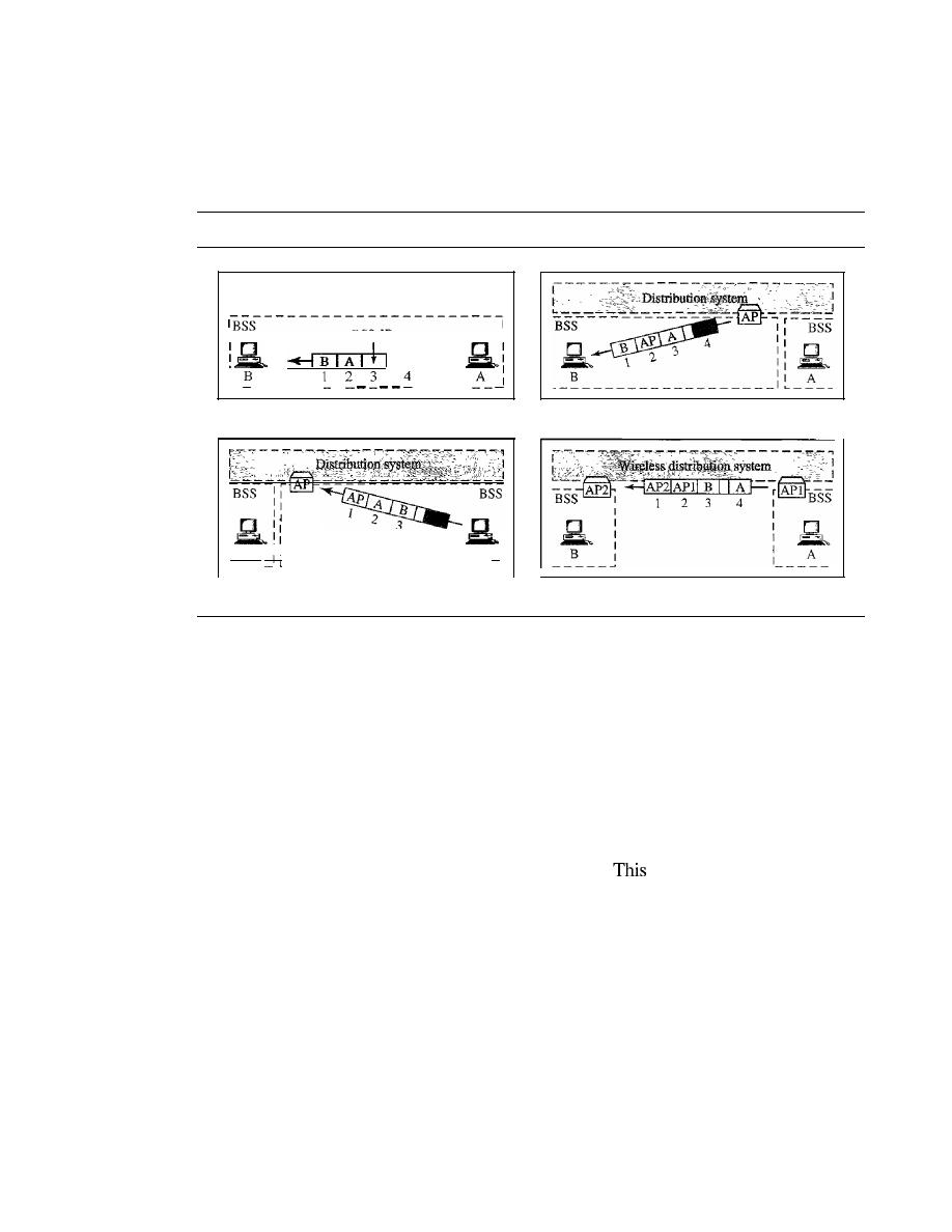
SECTION
14.1
IEEE 802.11
429
system
(From DS
=
0). The frame is going from one station in a BSS to another
without passing through the distribution system. The
ACK
frame should be sent to
the original sender. The addresses are shown in Figure 14.9.
Figure 14.9
Addressing mechanisms
I
BSS-ID
:_
_
a. Case 1
3
4
B
II
A
_ _ _
_
c. Case 3
b. Case 2
d. Case 4
o
Case 2: 01 In this case,
To DS
=
0 and
From DS
=
1. This means that the frame is
coming from a distribution system
(From
DS
=
1). The frame is coming from an
AP
and going to a station. The
ACK
should be sent to the
AP.
The addresses are as
shown in Figure 14.9. Note that address 3 contains the original sender of the frame
(in another BSS).
o
Case 3: 10 In this case,
To DS
=
1 and
From DS
=
O. This means that the frame is
going to a distribution system
(To DS
=
1). The frame is going from a station to an
AP.
The
ACK
is sent to the original station. The addresses are as shown in Figure 14.9.
Note that address 3 contains the final destination of the frame (in another BSS).
o
Case 4:11 In this case,
To DS
=
1 and
From DS
=
1.
is the case in which the distri-
bution system is also wireless. The frame is going from one AP to another AP in a wire-
less distribution system. We do not need to define addresses if the distribution system is
a wired LAN because the frame in these cases has the format of a wired LAN frame
(Ethernet, for example). Here, we need four addresses to define the original sender, the
final destination, and two intermediate APs. Figure 14.9 shows the situation.
Hidden and Exposed Station Problems
We referred to hidden and exposed station problems in the previous section.
It
is time
now to dicuss these problems and their effects.
Hidden Station Problem
Figure 14.10 shows an example of the hidden station
problem. Station B has a transmission range shown by the left oval (sphere in space);
every station in this range can hear any signal transmitted by station B. Station C has
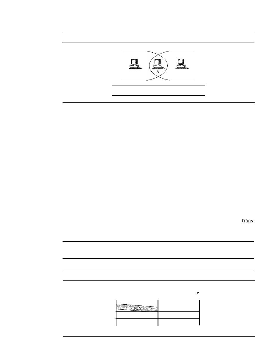
430
CHAPTER
14
WIRELESS LANs
Figure 14.10
Hidden station problem
Range
ofB
B
c
Range
ofC
Band Care hiddent from each other with respect to A.
a transmission range shown by the right oval (sphere in space); every station located
in this range can hear any signal transmitted by C. Station C is outside the transmis-
sion range of B; likewise, station B is outside the transmission range of C. Station A,
however, is in the area covered by both Band C; it can hear any signal transmitted by
B
or C.
Assume that station B is sending data to station
A.
In the middle of this transmission,
station C also has data to send to station A. However, station C is out of B's range and
transmissions from B cannot reach C. Therefore C thinks the medium is free. Station C
sends its data to A, which results in a collision at A because this station is receiving data
from both B and C. In this case, we say that stations Band C are hidden from each other
with respect to
A.
Hidden stations can reduce the capacity of the network because of the
possibility of collision.
The solution to the hidden station problem is the use of the handshake frames (RTS
and CTS) that we discussed earlier. Figure 14.11 shows that the RTS message from B
reaches A, but not C. However, because both Band C are within the range of A, the
CTS message, which contains the duration of data transmission from B to A reaches C.
Station C knows that some hidden station is using the channel and refrains from
mitting until that duration is over.
The CTS frame in CSMAICA handshake can prevent collision
from a hidden station.
Figure 14.11
Use of handshaking to prevent hidden station problem
B
A
C
CTS
CTS
Time
Time
Time
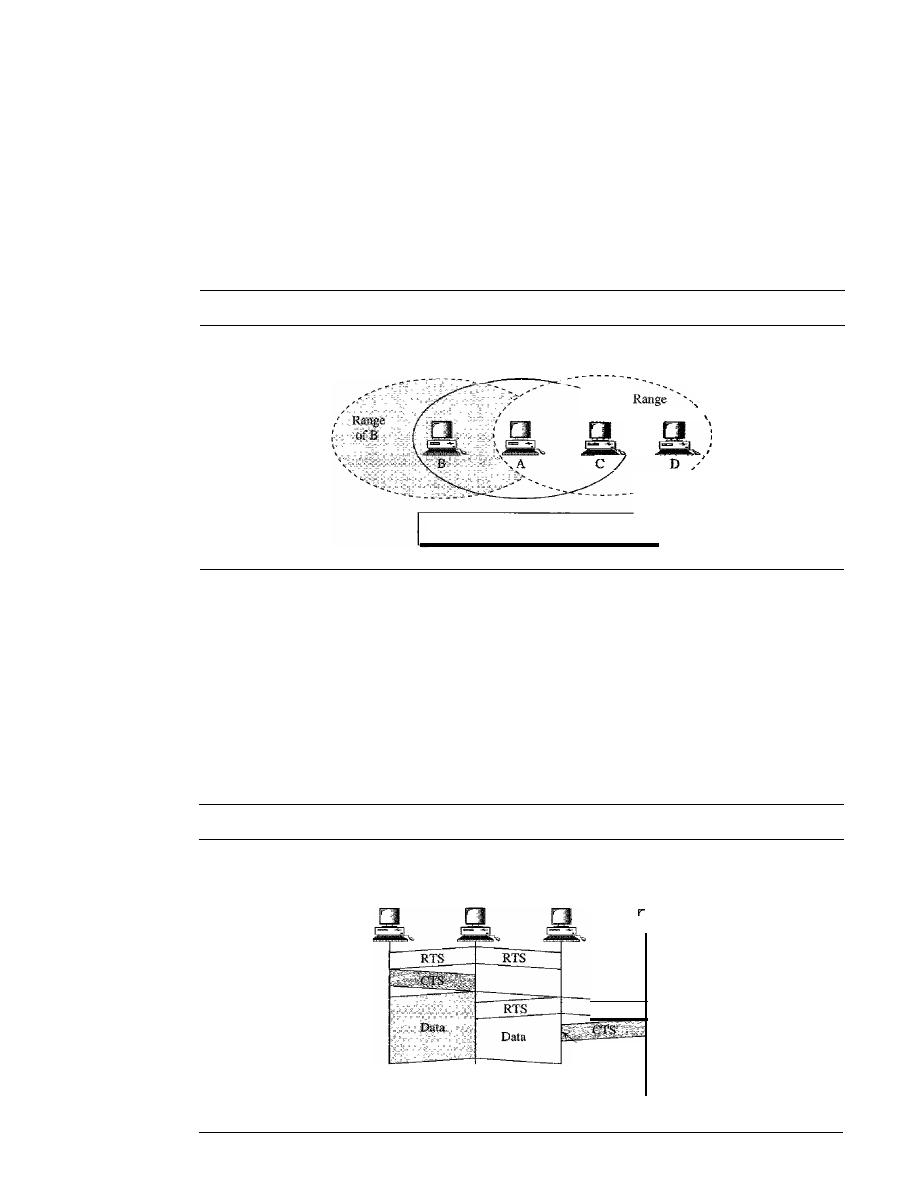
SECTION 14.1
IEEE 802.11
431
Exposed Station Problem
Now consider a situation that is the inverse of the previ-
ous one: the exposed station problem. In this problem a station refrains from using a
channel when it is, in fact, available.
In
Figure 14.12, station A is transmitting to station B.
Station C has some data to send to station D, which can be sent without interfering
with the transmission from A to B. However, station C is exposed to transmission from
A; it hears what A is sending and thus refrains from sending. In other words, C is too
conservative and wastes the capacity of the channel.
Figure
14.12
Exposed station problem
Range
of A
ofC
C is exposed to transmission from A to B.
The handshaking messages RTS and CTS cannot help in this case, despite what you
might think. Station C hears the RTS from A, but does not hear the CTS from
B.
Station C,
after hearing the RTS from A, can wait for a time so that the CTS from B reaches A; it then
sends an RTS to D to show that
it
needs to communicate with D. Both stations B and A
may hear this RTS, but station A is
in
the sending state, not the receiving state. Station B,
however, responds with a CTS. The problem is here.
If
station A has started sending its
data, station C cannot hear the CTS from station D because of the collision; it cannot send
its data to D.
It
remains exposed until A finishes sending its data as Figure 14.13 shows.
Figure
14.13
Use of handshaking in exposed station problem
B
Time
A
Time
Exposed to
A's transmission
C
RTS
Collision
here
Time
D
Time
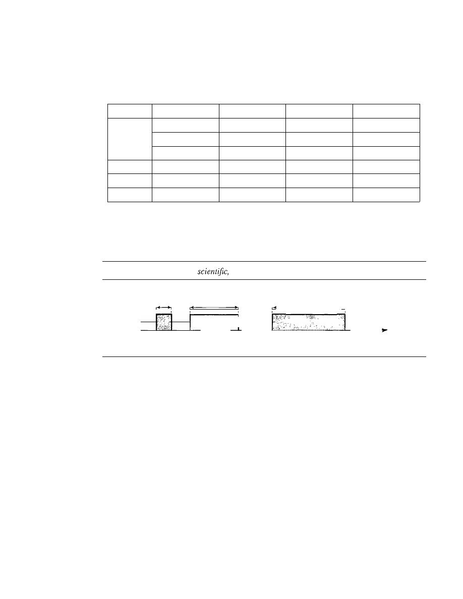
125
MHz
432
CHAPTER i4
WiRELESS LANs
Physical Layer
We discuss six specifications, as shown in Table 14.4.
Table 14.4
Physical layers
IEEE
Technique
Band
Modulation
Rate (Mbps)
802.11
FHSS
2.4 GHz
FSK
1 and 2
DSSS
2.4 GHz
PSK
1 and 2
Infrared
PPM
1 and 2
802.11a
OFDM
5.725 GHz
PSKorQAM
6 to 54
802.l1b
DSSS
2.4 GHz
PSK
5.5 and 11
802.1Ig
OFDM
2.4 GHz
Different
22 and 54
All implementations, except the infrared, operate in the
industrial, scientific,
and
medical (ISM)
band, which defines three unlicensed bands in the three ranges
902-928 MHz, 2.400--4.835 GHz, and 5.725-5.850 GHz, as shown in Figure 14.14.
Figure 14.14
industrial,
and medical (ISM) band
26
83.5
,MHz,
M H z ,
,
" I
,
;
.
902
928
2.4
2.4835
5.725
5.850
Frequency
MHz MHz GHz
GHz
GHz
GHz
IEEE 802.11 FHSS
IEEE 802.11 FHSS uses the frequency-hopping spread spectrum (FHSS) method as
discussed in Chapter 6. FHSS uses the 2.4-GHz ISM band. The band is divided into
79 subbands of 1 MHz (and some guard bands). A pseudorandom number generator
selects the hopping sequence. The modulation technique in this specification is either
two-level FSK or four-level FSK with I or 2 bitslbaud, which results in a data rate of 1
or 2 Mbps, as shown in Figure 14.15.
IEEE 802.11 DSSS
IEEE 802.11 DSSS uses the direct sequence spread spectrum (DSSS) method as dis-
cussed in Chapter 6. DSSS uses the 2.4-GHz ISM band. The modulation technique in this
specification is PSK at 1 Mbaud/s. The system allows 1 or 2 bitslbaud (BPSK or QPSK),
which results in a data rate of 1 or 2 Mbps, as shown in Figure 14.16.
IEEE 802.11
Infrared
IEEE 802.11 infrared uses infrared light in the range of 800 to 950 nm. The modulation
technique is called pulse position modulation (PPM). For a I-Mbps data rate, a 4-bit
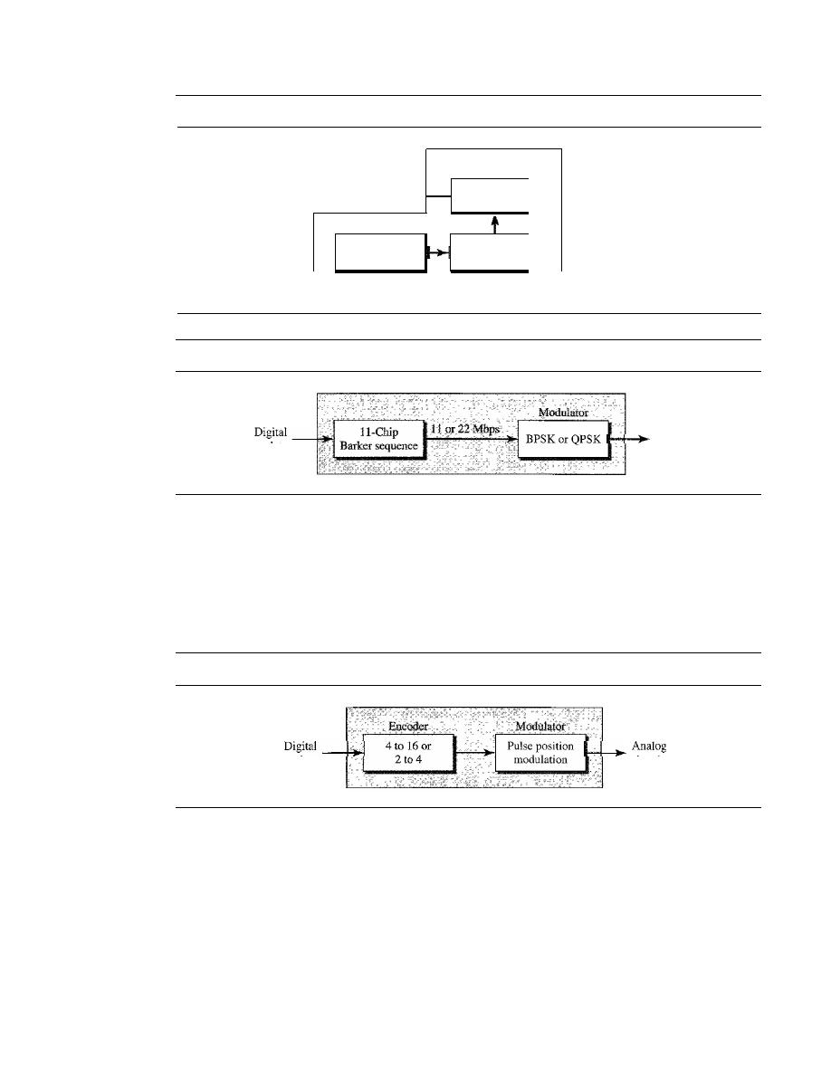
SECTION
14.1
IEEE 802.11
433
Figure 14.15
Physical layer of IEEE 802.11 FHSS
lor 2 Mbps
Modulator
Digital
2-Level or 4-1evell
data
FSK
I
Pseudorandom
Frequency
I
sequence
synthetizer
Figure 14.16
Physical layer of IEEE 802.11 DSSS
lor 2 Mbps
data
I-MHz
Analog
signal
II-MHz
Analog
signal
sequence is first mapped into a 16-bit sequence in which only one bit is set to 1 and the
rest are set to
O. For a 2-Mbps data rate, a 2-bit sequence is first mapped into a 4-bit
sequence in which only one bit is set to 1 and the rest are set to
O. The mapped
sequences are then converted to optical signals; the presence of light specifies 1, the
absence of light specifies
O. See Figure 14.17.
Figure 14.17
Physical layer of IEEE 802.11 infrared
lor 2 Mbps
data
signal
IEEE 802.lla OFDM
IEEE 802.Ila OFDM describes the
orthogonal frequency-division multiplexing
(OFDM) method for signal generation in a 5-GHz ISM band. OFDM is similar to
FDM as discussed in Chapter 6, with one major difference: All the subbands are used
by one source at a given time. Sources contend with one another at the data link layer
for access. The band is divided into 52 subbands, with 48 subbands for sending 48
groups of bits at a time and 4 subbands for control information. The scheme is similar
to ADSL, as discussed in Chapter 9. Dividing the band into subbands diminishes the
effects of interference.
If
the subbands are used randomly, security can also be increased.
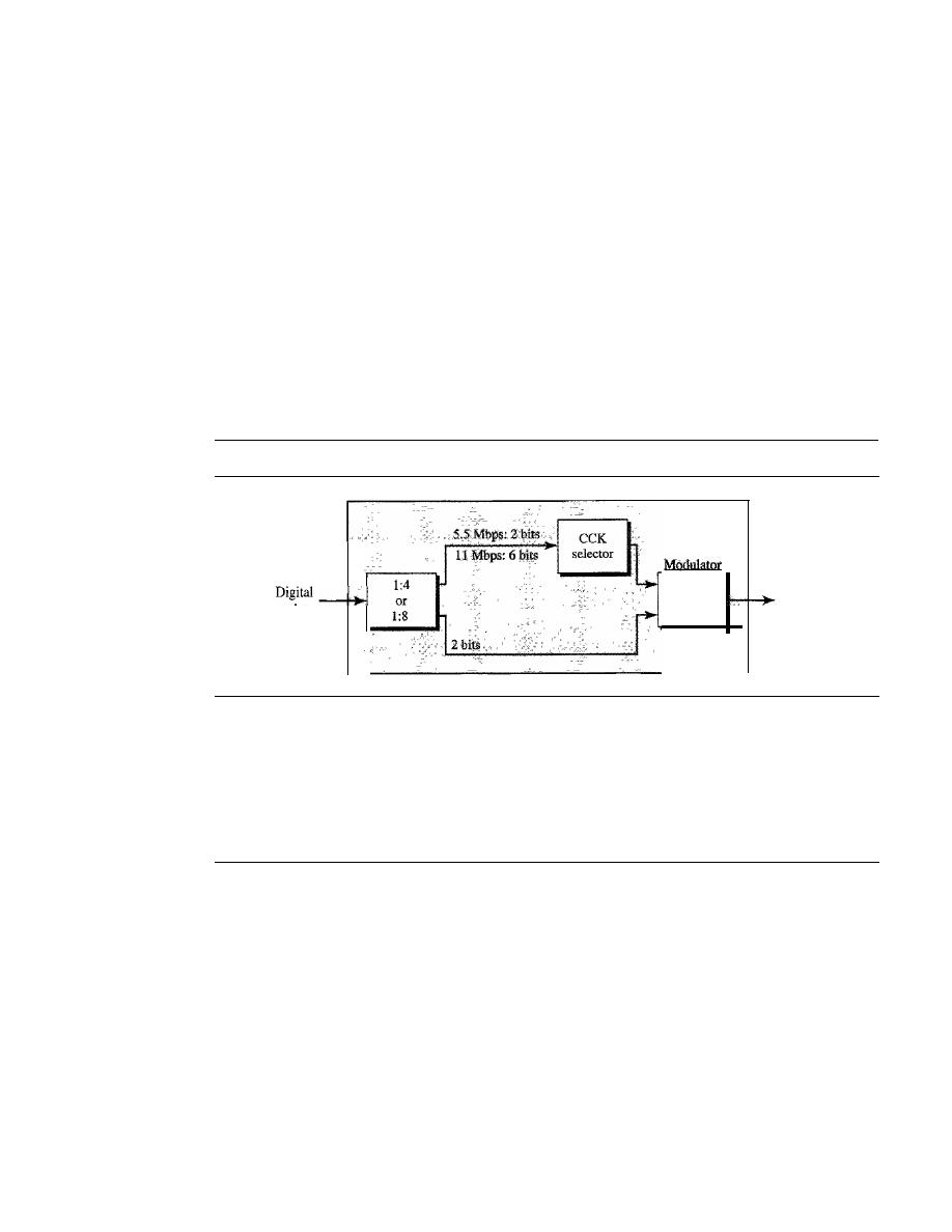
434
CHAPTER 14
WIRELESS LANs
OFDM uses PSK and QAM for modulation. The common data rates are 18 Mbps (PSK)
and 54 Mbps (QAM).
IEEE 802.llb DSSS
IEEE 802.11 b DSSS describes the
high-rate direct sequence spread spectrum
(HR-
DSSS) method for signal generation in the 2.4-GHz ISM band. HR-DSSS is similar to
DSSS except for the encoding method, which is called
complementary code keying
(CCK). CCK encodes 4 or 8 bits to one CCK symbol. To be backward compatible with
DSSS, HR-DSSS defines four data rates: 1,2, 5.5, and 11 Mbps. The first two use the
same modulation techniques as DSSS. The 5.5-Mbps version uses BPSK and transmits
at 1.375 Mbaudls with 4-bit CCK encoding. The II-Mbps version uses QPSK and trans-
mits at 1.375 Mbps with 8-bit CCK encoding. Figure 14.18 shows the modulation tech-
nique for this standard.
Figure 14.18
Physical layer ofIEEE 802.11b
5.5 or
II Mbps
data
QPSK
ll-MHz
Analog
signal
IEEE 802.11g
This new specification defines forward error correction and OFDM using the 2.4-GHz
ISM band. The modulation technique achieves a 22- or 54-Mbps data rate. It is backward-
compatible with 802.11 b, but the modulation technique is OFDM.
14.2
BLUETOOTH
Bluetooth
is a wireless LAN technology designed to connect devices of different func-
tions such as telephones, notebooks, computers (desktop and laptop), cameras, printers,
coffee makers, and so on. A Bluetooth LAN is an ad hoc network, which means that the
network is formed spontaneously; the devices, sometimes called gadgets, find each
other and make a network called a piconet. A Bluetooth LAN can even be connected to
the Internet if one of the gadgets has this capability. A Bluetooth LAN, by nature, can-
not be large.
If
there are many gadgets that try to connect, there is chaos.
Bluetooth technology has several applications. Peripheral devices such as a wire-
less mouse or keyboard can communicate with the computer through this technology.
Monitoring devices can communicate with sensor devices in a small health care center.
Home security devices can use this technology to connect different sensors to the main
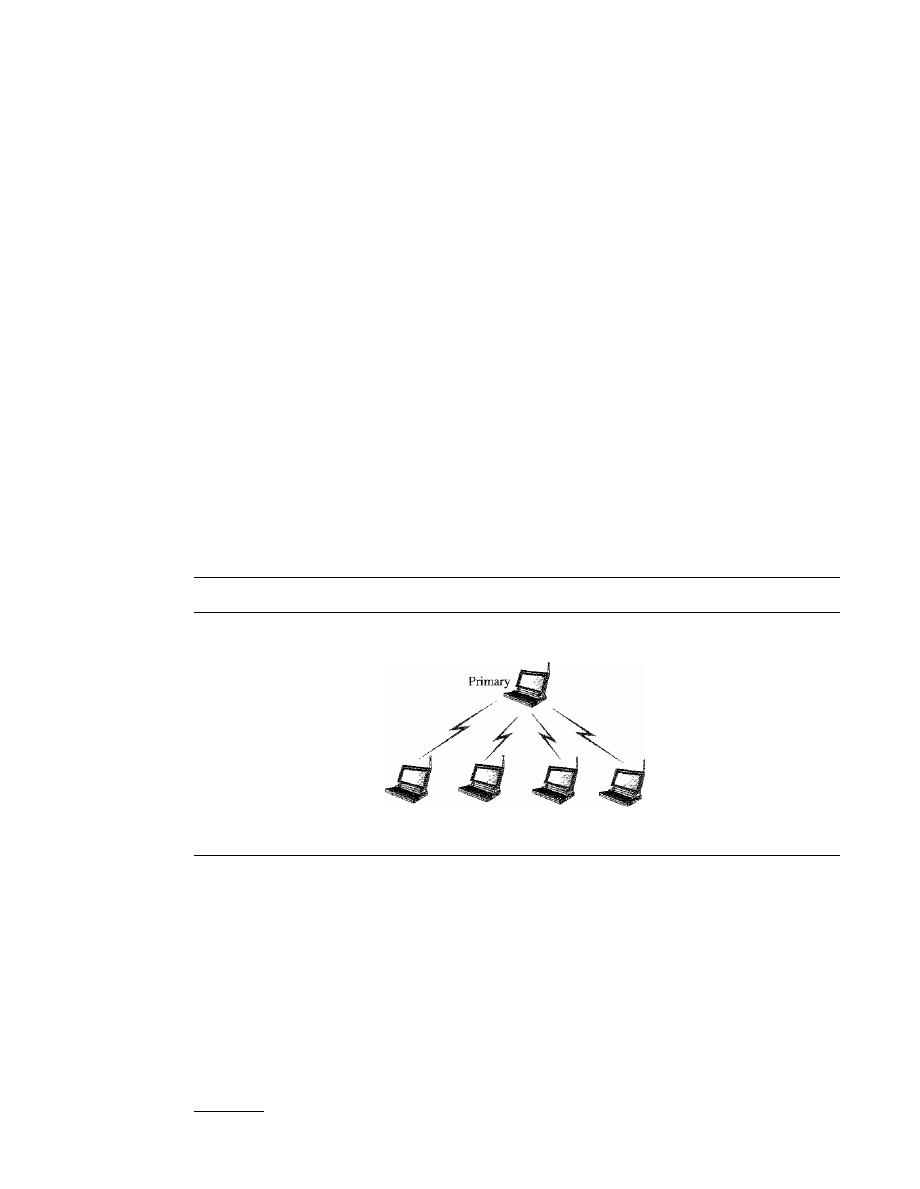
SECTION
14.2
BLUETOOTH
435
security controller. Conference attendees can synchronize their laptop computers at a
conference.
Bluetooth was originally started as a project by the Ericsson Company.
It
is named
for Harald Blaatand, the king of Denmark (940-981) who united Denmark and Norway.
Blaatand
translates to
Bluetooth
in English.
Today, Bluetooth technology is the implementation of a protocol defined by the
IEEE 802.15 standard. The standard defines a wireless personal-area network (PAN)
operable in an area the size of a room or a hall.
Architecture
Bluetooth defines two types of networks: piconet and scatternet.
Piconets
A Bluetooth network is called a
piconet, or a small net. A piconet can have up to eight
stations, one of which is called the
primary;
t
the rest are called
secondaries. All the
secondary stations synchronize their clocks and hopping sequence with the primary.
Note that a piconet can have only one primary station. The communication between the
primary and the secondary can be one-to-one or one-to-many. Figure 14.19 shows a
piconet.
Figure 14.19
Piconet
Piconet
-----------------------------
I
Secondary
Secondary
Secondary
Secondary
Although a piconet can have a maximum of seven secondaries, an additional eight
secondaries can be in the
parked state.
A secondary in a parked state is synchronized
with the primary, but cannot take part in communication until it is moved from the
parked state. Because only eight stations can be active in a piconet, activating a station
from the parked state means that an active station must go to the parked state.
Scat/ernet
Piconets can be combined to form what is called a
scatternet. A secondary station in
one piconet can be the primary in another piconet. This station can receive messages
tThe literature sometimes uses the terms master and slave instead of primary and secondary. We prefer the latter.
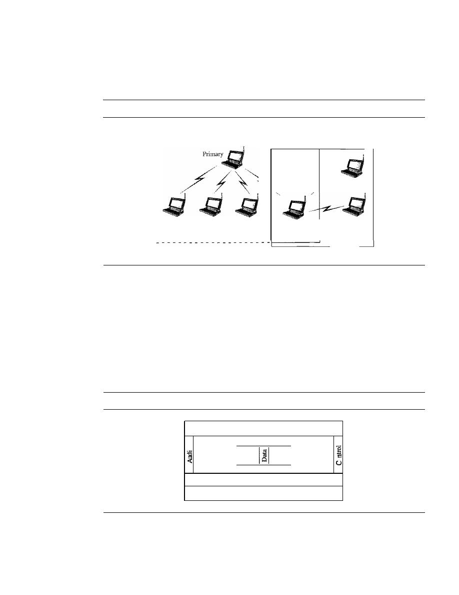
436
CHAPTER 14
WIRELESS LANs
from the primary in the first piconet (as a secondary) and, acting as a primary, deliver
them to secondaries in the second piconet. A station can be a member of two piconets.
Figure 14.20 illustrates a scatternet.
Figure 14.20
Scatternet
Piconet
Secondary
Secondary
Secondary
Primary/
Secondary
Secondary
Secondary
Piconet
Bluetooth Devices
A Bluetooth device has a built-in short-range radio transmitter. The current data rate is
1 Mbps with a 2.4-GHz bandwidth. This means that there is a possibility of interference
between the IEEE 802.11b wireless LANs and Bluetooth LANs.
Bluetooth
Layers
Bluetooth uses several layers that do not exactly match those of the Internet model we
have defined in this book. Figure 14.21 shows these layers.
Figure 14.21
Bluetooth layers
Applications
I
Profiles
I
0
0
I
L2CAPIayer
I
Baseband layer
Radio layer
Radio
Layer
The radio layer is roughly equivalent to the physical layer of the Internet model. Bluetooth
devices are low-power and have a range of 10 m.

SECTION
14.2
BLUETOOTH
437
Band
Bluetooth uses a 2.4-GHz ISM band divided into 79 channels of 1 MHz each.
FHSS
Bluetooth uses the frequency-hopping spread spectrum (FHSS) method in the phys-
ical layer to avoid interference from other devices or other networks. Bluetooth
hops 1600 times per second, which means that each device changes its modulation fre-
quency 1600 times per second. A device uses a frequency for only 625
(1/1600 s)
before it hops to another frequency; the dwell time is 625
Modulation
To transform bits to a signal, Bluetooth uses a sophisticated version of FSK, called
GFSK (FSK with Gaussian bandwidth filtering; a discussion of this topic is beyond the
scope of this book). GFSK has a can'ier frequency. Bit 1 is represented by a frequency
deviation above the carrier; bit
a
is represented by a frequency deviation below the
carrier. The frequencies, in megahertz, are defined according to the following formula
for each channel:
fc=2402+n
n
0, 1,2,3, ..., 78
For example, the first channel uses carrier frequency 2402 MHz (2.402 GHz), and the
second channel uses carrier frequency 2403 MHz (2.403 GHz).
Baseband Layer
The baseband layer is roughly equivalent to the MAC sublayer in LANs. The access
method is TDMA (see Chapter 12). The primary and secondary communicate with
each other using time slots. The length of a time slot is exactly the same as the dwell
time, 625
This means that during the time that one frequency is used, a sender sends
a frame to a secondary, or a secondary sends a frame to the primary. Note that the com-
munication is only between the primary and a secondary; secondaries cannot communi-
cate directly with one another.
TDMA
Bluetooth uses a form of TDMA (see Chapter 12) that is called TDD-TDMA (time-
division duplex TDMA). TDD-TDMA is a kind of half-duplex communication in
which the secondary and receiver send and receive data, but not at the same time (half-
duplex); however, the communication for each direction uses different hops. This is
similar to walkie-talkies using different carrier frequencies.
Single-Secondary Communication
If the piconet has only one secondary, the TDMA
operation is very simple. The time is divided into slots of 625
The primary uses even-
numbered slots (0, 2, 4, ...); the secondary uses odd-numbered slots (1, 3, 5, ...).
TDD-TDMA allows the primary and the secondary to communicate in half-duplex mode.
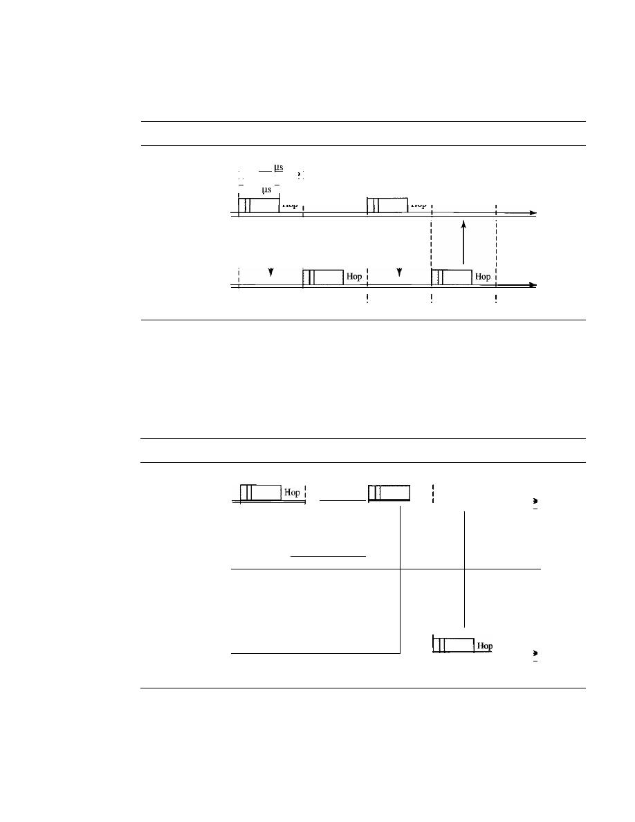
fO
438
CHAPTER
14
WIRELESS LANs
In slot 0, the primary sends, and the secondary receives;
in
slot 1, the secondary sends, and
the primary receives. The cycle is repeated. Figure 14.22 shows the concept.
Figure 14.22
Single-secondary communication
I
625
I
i '
i
I,
.1
I
: 366
I :
I
I
Hop
I
Hop:
Primary
l
i t
1
I
Time
,
I :
Secondary
I
I
I
I
Time
I
fl
f2
f3
Multiple-Secondary Communication
The process is a little more involved
if
there is
more than one secondary in the piconet. Again, the primary uses the even-numbered slots,
but a secondary sends in the next odd-numbered slot if the packet in the previous slot was
addressed to it. All secondaries listen on even-numbered slots, but only one secondary
sends in any odd-numbered slot. Figure 14.23 shows a scenario.
Figure 14.23
Multiple-secondary communication
I
I
I
I
Hop
Primary
I
j
I
1
I
Time
I
I
I
I
I
I
I
I
I
I
I
I
I
I
I
Hop
I
Secondary 1
I
I
Time
I
I
I
I
I
I
I
Secondary 2
I
I
f3
Time
fO
fl
f2
J
Let us elaborate on the figure.
1. In slot 0, the primary sends a frame to secondary 1.
2. In slot 1, only secondary I sends a frame to the primary because the previous frame
was addressed to secondary 1; other secondaries are silent.

SECTION
14.2
BLUETOOTH
439
3. In slot 2, the primary sends a frame to secondary 2.
4. In slot 3, only secondary 2 sends a frame to the primary because the previous frame
was addressed to secondary 2; other secondaries are silent.
5. The cycle continues.
We can say that this access method is similar to a poll/select operation with reservations.
When the primary selects a secondary, it also polls it. The next time slot is reserved for
the polled station to send its frame.
If
the polled secondary has no frame to send, the
channel is silent.
Physical Links
Two types of links can be created between a primary and a secondary: SCQ links and
ACL links.
sca
A synchronous connection-oriented
(SeQ)
link is used when avoiding latency
(delay in data delivery) is more important than integrity (error-free delivery). In an
SCQ link, a physical link is created between the primary and a secondary by reserving
specific slots at regular intervals. The basic unit of connection is two slots, one for each
direction. If a packet is damaged, it is never retransmitted. SCQ is used for real-time
audio where avoiding delay is all-important. A secondary can create up to three SCQ
links with the primary, sending digitized audio (PCM) at 64 kbps in each link.
ACL
An asynchronous connectionless link (ACL) is used when data integrity is
more important than avoiding latency. In this type of link, if a payload encapsulated
in the frame is corrupted, it is retransmitted. A secondary returns an ACL frame in
the available odd-numbered slot if and only if the previous slot has been addressed
to it. ACL can use one, three, or more slots and can achieve a maximum data rate of
721 kbps.
Frame Format
A frame in the baseband layer can be one of three types: one-slot, three-slot, or five-slot.
A slot, as we said before, is 625
However, in a one-slot frame exchange, 259
is
needed for hopping and control mechanisms. This means that a one-slot frame can last
only 625 - 259, or 366
With a I-MHz bandwidth and 1 bit/Hz, the size of a one-slot
frame is 366 bits.
A three-slot frame occupies three slots. However, since 259
is used for hopping,
the length of the frame is 3 x 625 - 259
=
1616
or 1616 bits. A device that uses a
three-slot frame remains at the same hop (at the same carrier frequency) for three slots.
Evcn though only onc hop numbcr is used, three hop numbers are consumed. That means
the hop number for each frame is equal to the first slot of the frame.
A five-slot frame also uses 259 bits for hopping, which means that the length of the
frame is 5 x 625 - 259
=
2866 bits.
Figure 14.24 shows the format of the three frame types.
The following describes each field:
o
Access code. This 72-bit field normally contains synchronization bits and the
identifier of the primary to distinguish the frame of one piconet from another.
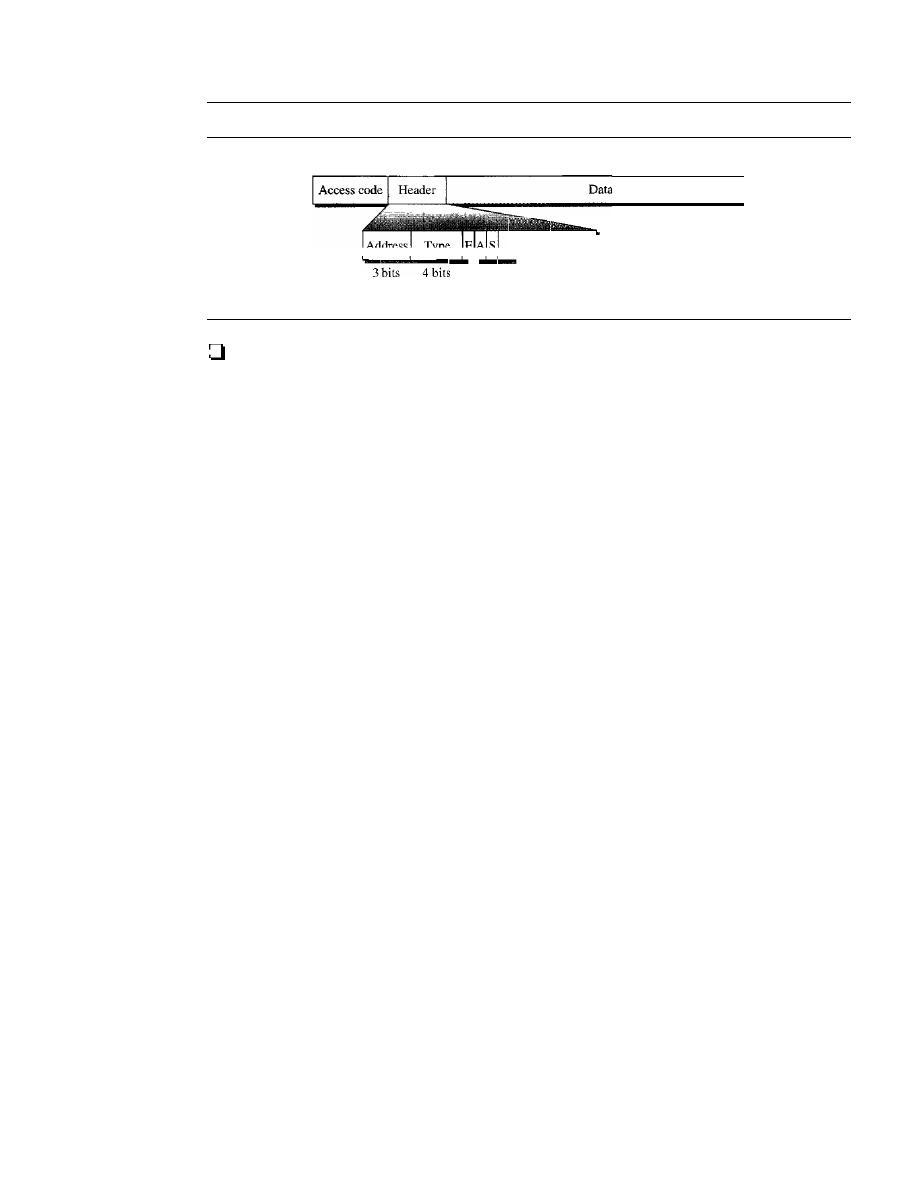
440
CHAPTER
14
WIRELESS LANs
Figure 14.24
Framefannat types
72 bits
54 bits
o
to
N
bits
N
=
240 for I-sIal frame
N
=
1490 for 3-slot frame
l...l l
-S-b-it-s- -
N =
2740 for 5-slot frame
This IS-bit part is repeated 3 times.
Header. This 54-bit field is a repeated I8-bit pattern. Each pattern has the follow-
ing subfields:
1.
Address. The 3-bit address subfield can define up to seven secondaries
(l
to 7).
If the address is zero, it is used for broadcast communication from the primary
to all secondaries.
2. Type. The 4-bit type subfield defines the type of data coming from the upper
layers. We discuss these types later.
3.
F.
This I-bit subfield is for flow control. When set (I), it indicates that the device
is unable to receive more frames (buffer is full).
4. A. This I-bit subfield is for acknowledgment. Bluetooth uses Stop-and-Wait
ARQ; I bit is sufficient for acknowledgment.
5. S. This I-bit subfield holds a sequence number. Bluetooth uses Stop-and-Wait
ARQ; I bit is sufficient for sequence numbering.
6. HEC. The 8-bit header error correction subfield is a checksum to detect errors
in each 18-bit header section.
The header has three identical 18-bit sections. The receiver compares these three
sections, bit by bit. If each of the corresponding bits is the same, the bit is accepted;
if not, the majority opinion rules. This is a form of forward error correction (for the
header only). This double error control is needed because the nature of the commu-
nication, via air, is very noisy. Note that there is no retransmission in this sublayer.
o
Payload. This subfield can be 0 to 2740 bits long.
It
contains data or control
information corning from the upper layers.
L2CAP
The Logical Link Control and Adaptation Protocol, or L2CAP (L2 here means LL),
is roughly equivalent to the LLC sublayer in LANs.
It
is used for data exchange on an
ACL link; SCQ channels do not use L2CAP. Figure 14.25 shows the format of the data
packet at this level.
The I6-bit length field defines the size of the data, in bytes, coming from the upper
layers. Data can be up to 65,535 bytes. The channel ID (CID) defines a unique identi-
fier for the virtual channel created at this level (see below).
The L2CAP has specific duties: multiplexing, segmentation and reassembly, quality
of service (QoS), and group management.

SECTION
14.3
RECOMMENDED READING
441
Figure 14.25
L2CAP data packetfarmat
2 bytes
2 bytes
0 to 65,535 bytes
Length
I
Channel ID
1
D_at_a_an_d_co_n_tro_l
_
Multiplexing
The L2CAP can do multiplexing. At the sender site, it accepts data from one of the
upper-layer protocols, frames them, and delivers them to the baseband layer. At the
receiver site, it accepts a frame from the baseband layer, extracts the data, and delivers
them to the appropriate protocol layer.
It
creates a kind of virtual channel that we will
discuss in later chapters on higher-level protocols.
Segmentation and Reassembly
The maximum size of the payload field in the baseband layer is 2774 bits, or 343 bytes.
This includes 4 bytes to define the packet and packet length. Therefore, the size of the
packet that can arrive from an upper layer can only be 339 bytes. However, application
layers sometimes need to send a data packet that can be up to 65,535 bytes (an Internet
packet, for example). The L2CAP divides these large packets into segments and adds
extra information to define the location of the segments in the original packet. The
L2CAP segments the packet at the source and reassembles them at the destination.
QoS
Bluetooth allows the stations to define a quality-of-service level. We discuss quality of
service in Chapter 24. For the moment, it is sufficient to know that if no quality-of-service
level is defined, Bluetooth defaults to what is called best-effort service; it will do its best
under the circumstances.
Group Management
Another functionality of L2CAP is to allow devices to create a type of logical addressing
between themselves. This is similar to multicasting. For example, two or three secondary
devices can be part of a multicast group to receive data from the primary.
Other Upper Layers
Bluetooth defines several protocols for the upper layers that use the services of L2CAP;
these protocols are specific for each purpose.
14.3
RECOMMENDED READING
For more details about subjects discussed in this chapter, we recommend the follow-
ing books and sites. The items in brackets [...] refer to the reference list at the end of
the text.

442
CHAPTER
14
WIRELESS LANs
Books
Wireless LANs and Bluetooth are discussed in several books including [Sch03] and
[Gas02]. Wireless LANs are discussed in Chapter 15 of [For03], Chapter 17 of [Sta04],
Chapters 13 and 14 of [Sta02], and Chapter 8 of [Kei021. Bluetooth is discussed in
Chapter 15 of [Sta02] and Chapter 15 of [For03].
14.4
KEY TERMS
access point (AP)
asynchronous connectionless link
(ACL)
basic service set (B SS)
beacon frame
Bluetooth
BSS-transition mobility
complementary code keying (CCK)
direct sequence spread spectrum (OSSS)
distributed coordination function (OCF)
distributed interframe space (OIFS)
ESS-transition mobility
extended service set (ESS)
frequency-hopping spread spectrum
(FHSS)
handshaking period
high-rate direct sequence spread spectrum
(HR-OSSS)
IEEE 802.11
Logical Link Control and Adaptation
Protocol (L2CAP)
network allocation vector (NAV)
no-transition mobility
orthogonal frequency-division
multiplexing (OFOM)
piconet
point coordination function (PCF)
primary
pulse position modulation (PPM)
repetition interval
scatternet
secondary
short interframe space (SIFS)
synchronous connection-oriented
(SCO)
TDD-TOMA (time-division duplex
TOMA)
wireless LAN
14.5
SUMMARY
o
The IEEE 802.11 standard for wireless LANs defines two services: basic service
set (BSS) and extended service set (ESS).
o
The access method used in the distributed coordination function (OCF) MAC sub-
layer is
CSMAICA.
o
The access method used in the point coordination function (PCF) MAC sublayer is
polling.
o
The network allocation vector (NAV) is a timer used for collision avoidance.
o
The MAC layer frame has nine fields. The addressing mechanism can include up to
four addresses.
o
Wireless LANs use management frames, control frames, and data frames.
SECTION
14.6
PRACTICE SET
443
o
IEEE 802.11 defines several physical layers, with different data rates and modulating
techniques.
o
Bluetooth is a wireless LAN technology that connects devices (called gadgets) in a
small area.
o
A Bluetooth network is called a piconet. Multiple piconets fonn a network called a
scatternet.
o
A Bluetooth network consists of one primary device and up to seven secondary
devices.
14.6
PRACTICE SET
Review Questions
1. What is the difference between a BSS and an ESS?
2. Discuss the three types of mobility in a wireless LAN.
3. How is OFDM different from FDM?
4.
What is the access method used by wireless LANs?
5. What is the purpose of the NAV?
6.
Compare a piconet and a scatternet.
7.
Match the layers in Bluetooth and the Internet model.
8. What are the two types of links between a Bluetooth primary and a Bluetooth
secondary?
9.
In multiple-secondary communication, who uses the even-numbered slots and who
uses the odd-numbered slots?
10. How much time in a Bluetooth one-slot frame is used for the hopping mechanism?
What about a three-slot frame and a five-slot frame?
Exercises
1].
Compare and contrast
CSMAlCD
with
CSMAICA.
12. Use Table 14.5 to compare and contrast the fields in IEEE 802.3 and 802.11.
Table
14.5
Exercise 12
Fields
IEEE 802.3 Field Size
IEEE 802.11 Field Size
Destination address
Source address
Address 1
Address 2
Address 3
Address 4
FC

444
CHAPTER
14
WIRELESS LANs
Table 14.5
Exercise
12
(continued)
..
..
-_.__.
Fields
IEEE 802.3 Field Size
IEEE 802.11 Field Size
D/ID
SC
PDU length
Data and padding
Frame body
FCS (CRC)
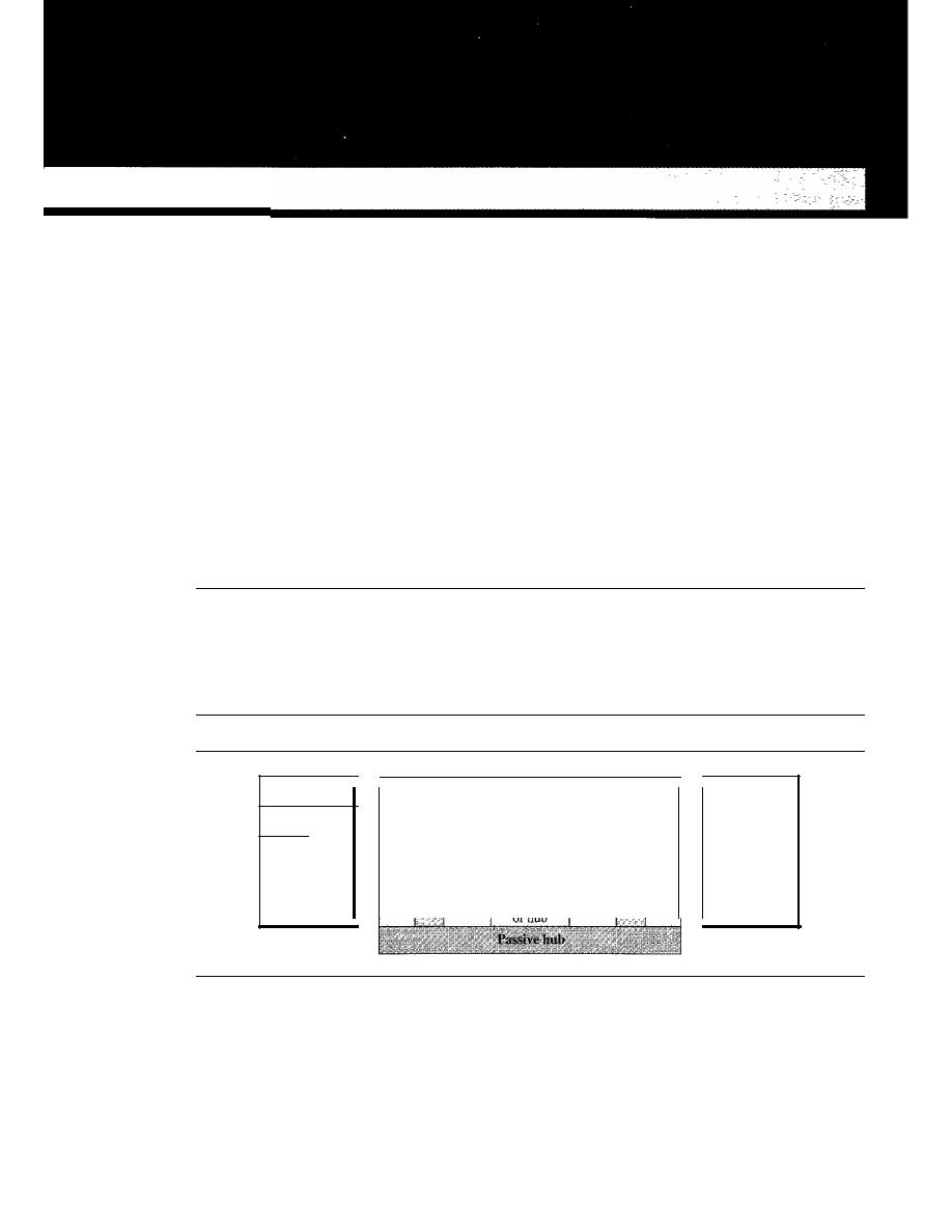
CHAPTER 15
Connecting LANs, Backbone
Networks, and Virtual LANs
LANs do not normally operate in isolation. They are connected to one another or to the
Internet. To connect LANs, or segments ofLANs, we use connecting devices. Connecting
devices can operate in different layers of the Internet model. In this chapter, we discuss
only those that operate in the physical and data link layers; we discuss those that operate
in the first three layers in Chapter 19.
After discussing some connecting devices, we show how they are used to create
backbone networks. Finally, we discuss virtual local area networks (VLANs).
15.1
CONNECTING DEVICES
In
this section, we divide connecting devices into five different categories based on the
layer
in
which they operate
in
a network, as shown
in
Figure 15.1.
Figure 15.1
Five categories of connecting devices
Application
Application
Gateway
Transport
Transport
Network
Network
Data link
Data link
Physical
Physical
The five categories contain devices which can be defined as
1. Those which operate below the physical layer such as a passive hub.
2. Those which operate at the physical layer (a repeater or an active hub).
3. Those which operate at the physical and data link layers (a bridge or a two-layer
switch).
445
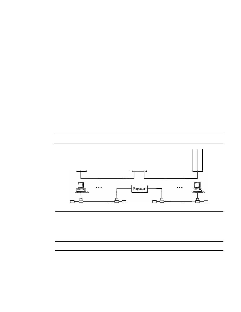
446
CHAPTER
15
CONNECTING LANs, BACKBONE NETWORKS, AND VIRTUAL LANs
4. Those which operate at the physical, data link, and network layers (a router or a
three-layer switch).
5. Those which can operate at all five layers (a gateway).
Passive Hubs
A passive hub is just a connector. It connects the wires coming from different branches.
In a star-topology Ethernet LAN, a passive hub is just a point where the signals coming
from different stations collide; the hub is the collision point. This type of a hub is part
of the media; its location in the Internet model is below the physical layer.
Repeaters
A
repeater is a device that operates only in the physical layer. Signals that carry infor-
mation within a network can travel a fixed distance before attenuation endangers the
integrity of the data. A repeater receives a signal and, before it becomes too weak or
corrupted, regenerates the original bit pattern. The repeater then sends the refreshed
signal. A repeater can extend the physical length of a LAN, as shown in Figure 15.2.
Figure 15.2
A repeater connecting two segments of a LAN
5
5
4
4
3
3
2
2
I
1
Segment I
Segment 2
A repeater does not actually connect two LANs; it connects two segments of the
same LAN. The segments connected are still part of one single LAN. A repeater is not
a device that can connect two LANs of different protocols.
A
repeater connects segments of a LAN.
A repeater can overcome the 10Base5 Ethernet length restriction. In this standard,
the length of the cable is limited to 500 m. To extend this length, we divide the cable
into segments and install repeaters between segments. Note that the whole network is
still considered one LAN, but the portions of the network separated by repeaters are
called segments. The repeater acts as a two-port node, but operates only in the physical
layer. When it receives a frame from any of the ports, it regenerates and forwards it to
the other port.
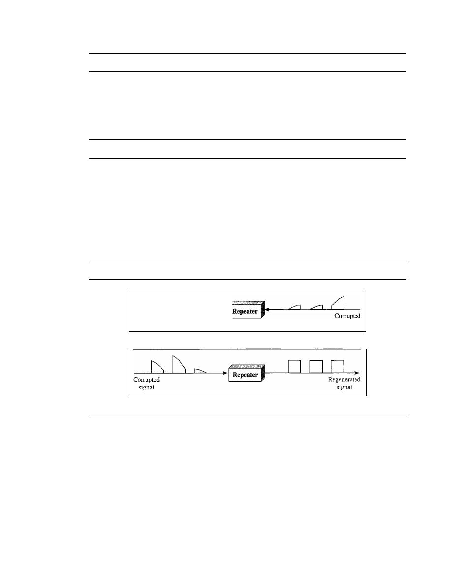
SECTION
15.1
CONNECTING DEVICES
447
A repeater forwards every frame; it has no filtering capability.
It
is tempting to compare a repeater to an amplifier, but the comparison is inaccurate.
An amplifier cannot discriminate between the intended signal and noise; it amplifies
equally everything fed into it. A repeater does not amplify the signal; it regenerates the
signal. When it receives a weakened or corrupted signal, it creates a copy, bit for bit, at
the original strength.
A repeater is a regenerator, not an amplifier.
The location of a repeater on a
link
is vital. A repeater must be placed so that a sig-
nal reaches it before any noise changes the meaning of any of its bits. A little noise can
alter the precision of a bit's voltage without destroying its identity (see Figure 15.3). If
the corrupted bit travels much farther, however, accumulated noise can change its
meaning completely. At that point, the original voltage is not recoverable, and the error
needs to be corrected. A repeater placed on the line before the legibility of the signal
becomes lost can still read the signal well enough to determine the intended voltages
and replicate them in their original form.
Figure 15.3
Function of a repeater
signal
signal
a. Right-to-teft transmission.
b. Left-to·right transmission.
Active Hubs
An active hub is actually a multipart repeater.
It
is normally used to create connections
between stations in a physical star topology. We have seen examples of hubs in some
Ethernet implementations (lOBase-T, for example). However, hubs can also be used to
create multiple levels of hierarchy, as shown in Figure 15.4. The hierarchical use of
hubs removes the length limitation of 10Base-T (100 m).
Bridges
A bridge operates in both the physical and the data link layer. As a physical layer
device, it regenerates the signal it receives. As a data link layer device, the bridge can
check the physical (MAC) addresses (source and destination) contained in the frame.
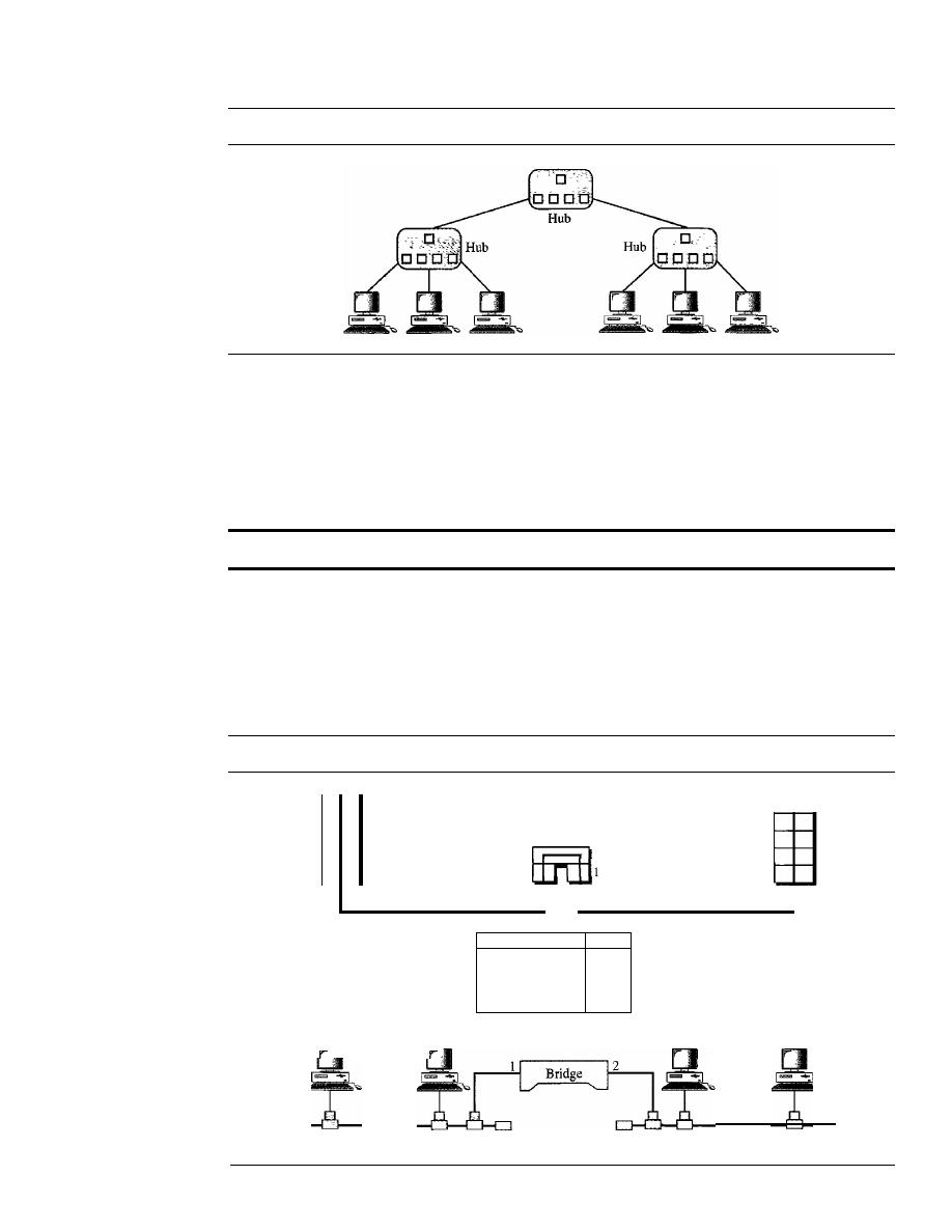
448
CHAPTER
15
CONNECTING LANs, BACKBONE NETWORKS, AND VIRTUAL LANs
Figure 15.4
A hierarchy of hubs
Filtering
One may ask, What is the difference in functionality between a bridge and a repeater?
A bridge has filtering capability. It can check the destination address of a frame and
decide if the frame should be forwarded or dropped. If the frame is to be forwarded, the
decision must specify the port. A bridge has a table that maps addresses to ports.
A bridge has a table nsed in filtering decisions.
Let us give an example. In Figure 15.5, two LANs are connected by a bridge.
If
a
frame destined for station 712B13456142 arrives at port 1, the bridge consults its table to
find the departing port. According to its table, frames for 7l2B 13456142 leave through
port 1; therefore, there is no need for forwarding, and the frame is dropped. On the
other hand, if a frame for 712B13456141 arrives at port 2, the departing port is port 1
Figure 15.5
A bridge connecting two LANs
5
4
3
2
1
2
2
1
5
4
3
2
I
Address
Port
71:2B: 13:45:61:41
1
71:2B: 13:45:61:42
1
64:2B: 13:45:61:12
2
64:28:13:45:61:13
2
Bridge Table
64:2B: 13:45:61: 12 64:2B: 13:45:61: 13
LAN 2
LAN 1
71:28: 13:45:61:41 71 :2B: 13:45:61:42

SECTION
15.1
CONNECTING DEVICES
449
and the frame is forwarded. In the first case, LAN 2 remains free of traffic; in the sec-
ond case, both LANs have traffic. In our example, we show a two-port bridge; in reality
a bridge usually has more ports.
Note also that a bridge does not change the physical addresses contained in the
frame.
A bridge does not change the physical (MAC) addresses in a frame.
Transparent Bridges
A transparent bridge is a bridge in which the stations are completely unaware of the
bridge's existence. If a bridge is added or deleted from the system, reconfiguration of
the stations is unnecessary. According to the IEEE 802.1 d specification, a system
equipped with transparent bridges must meet three criteria:
I.
Frames must be forwarded from one station to another.
2. The forwarding table is automatically made by learning frame movements in the
network.
3. Loops in the system must be prevented.
Forwarding
A transparent bridge must correctly forward the frames, as discussed in
the previous section.
Learning
The earliest bridges had forwarding tables that were static. The systems
administrator would manually enter each table entry during bridge setup. Although the
process was simple, it was not practical.
If
a station was added or deleted, the table had to
be modified manually. The same was true if a station's MAC address changed, which is
not a rare event. For example, putting in a new network card means a new MAC address.
A better solution to the static table is a dynamic table that maps addresses to ports
automatically. To make a table dynamic, we need a bridge that gradually learns from
the frame movements. To do this, the bridge inspects both the destination and the
source addresses. The destination address is used for the forwarding decision (table
lookup); the source address is used for adding entries to the table and for updating pur-
poses. Let us elaborate on this process by using Figure 15.6.
1. When station A sends a frame to station D, the bridge does not have an entry for
either D or
A.
The frame goes out from all three ports; the frame floods the net-
work. However, by looking at the source address, the bridge learns that station A
must be located on the LAN connected to port 1. This means that frames destined
for A, in the future, must be sent out through port 1. The bridge adds this entry to
its table. The table has its first entry now.
2. When station E sends a frame to station A, the bridge has an entry for A, so it for-
wards the frame only to port 1. There is no flooding. In addition, it uses the source
address of the frame, E, to add a second entry to the table.
3. When station B sends a frame to C, the bridge has no entry for C, so once again it
floods the network and adds one more entry to the table.
4. The process of learning continues as the bridge forwards frames.
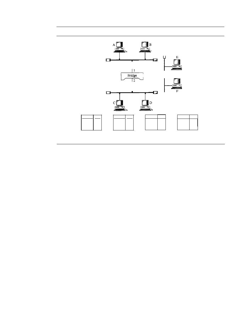
450
CHAPTER
15
CONNECTING LANs, BACKBONE NETWORKS, AND VIRTUAL LANs
Figure 15.6
A learning bridge and the process of learning
3
1--------1
LAN 2
LAN 1
LAN 3
Address Port
Address Port
A
1
Address Port
A
1
E
3
Address Port
A
1
E
3
B
I
a. Original
b. After A sends
a frame to D
c. After E sends
a frame to A
d. After B sends
a frame to C
Loop Problem
Transparent bridges work fine as long as there are no redundant
bridges in the system. Systems administrators, however, like to have redundant bridges
(more than one bridge between a pair of LANs) to make the system more reliable.
If
a
bridge fails, another bridge takes over until the failed one is repaired or replaced.
Redundancy can create loops in the system, which is very undesirable. Figure 15.7
shows a very simple example of a loop created in a system with two LANs connected
by two bridges.
1. Station A sends a frame to station D. The tables of both bridges are empty. Both
forward the frame and update their tables based on the source address A.
2. Now there are two copies of the frame on LAN 2. The copy sent out by bridge 1 is
received by bridge 2, which does not have any information about the destination
address D; it floods the bridge. The copy sent out by bridge 2 is received by bridge 1
and is sent out for lack of information about D. Note that each frame is handled
separately because bridges, as two nodes on a network sharing the medium, use an
access method such as CSMA/CD. The tables of both bridges are updated, but still
there is no information for destination D.
3. Now there are two copies of the frame on LAN 1. Step 2 is repeated, and both copies
flood the network.
4. The process continues on and on. Note that bridges are also repeaters and regen-
erate frames. So in each iteration, there are newly generated fresh copies of the
frames.
To solve the looping problem, the IEEE specification requires that bridges use the
spanning tree algorithm to create a loopless topology.
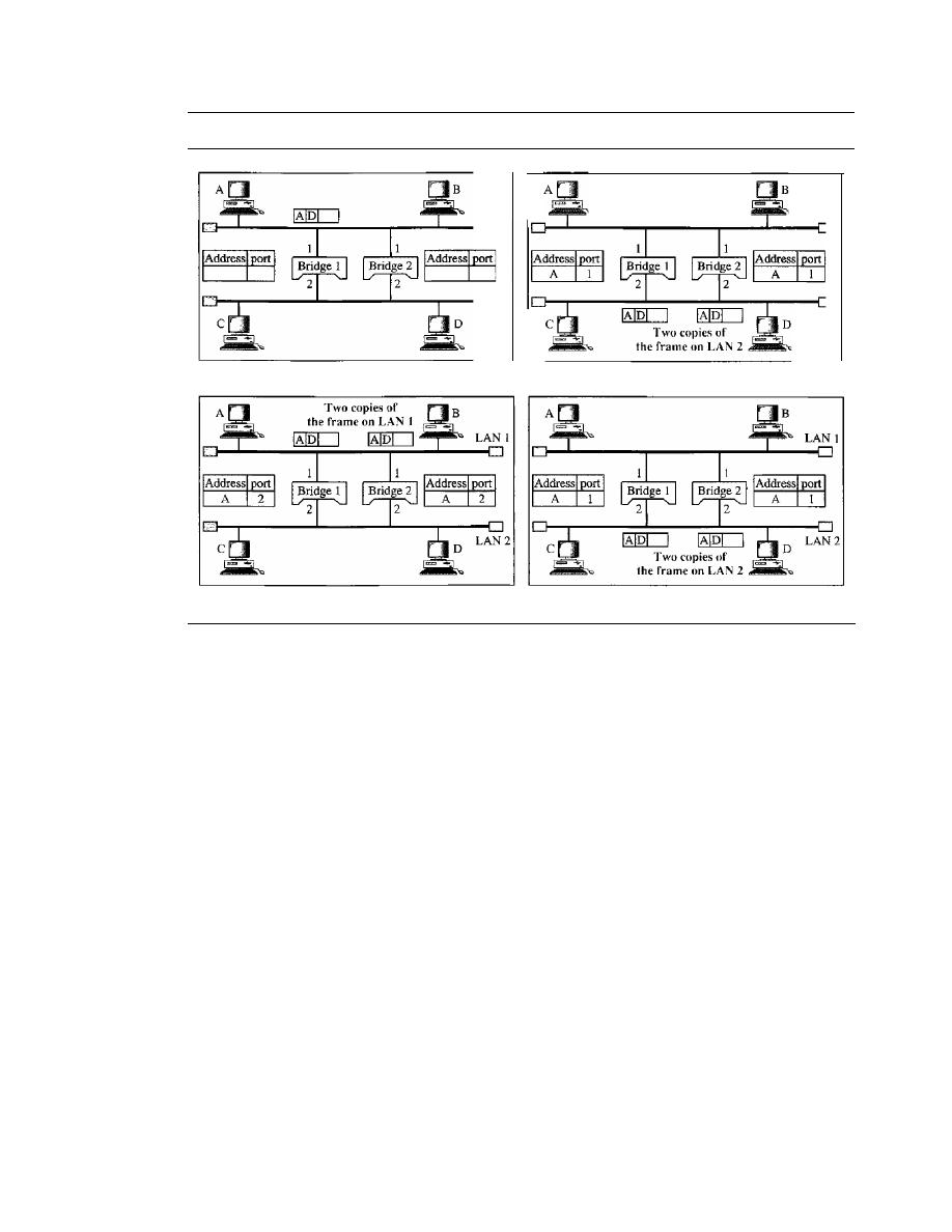
SECTION
15.1
CONNECTING DEVICES
451
Figure 15.7
Loop problem in a learning bridge
LAN 1
LAN 1
LAN 2
LAN 2
a. Station A sends a frame to station D
b. Both bridges forward the frame
c. Both bridges forward the frame
d. Both bridges forward the frame
Spanning Tree
In graph theory, a
spanning tree
is a graph in which there is no loop. In a bridged
LAN, this means creating a topology in which each LAN can be reached from any
other LAN through one path only (no loop). We cannot change the physical topology of
the system because of physical connections between cables and bridges, but we can
create a logical topology that overlays the physical one. Figure 15.8 shows a system
with four LANs and five bridges. We have shown the physical system and its represen-
tation in graph theory. Although some textbooks represent the LANs as nodes and the
bridges as the connecting arcs, we have shown both LANs and bridges as nodes. The
connecting arcs show the connection of a LAN to a bridge and vice versa. To find
the spanning tree, we need to assign a cost (metric) to each arc. The interpretation of
the cost is left up to the systems administrator.
It
may be the path with minimum hops
(nodes), the path with minimum delay, or the path with maximum bandwidth.
If
two
ports have the same shortest value, the systems administrator just chooses one. We have
chosen the minimum hops. However, as we will see in Chapter 22, the hop count is nor-
mally 1 from a bridge to the LAN and 0 in the reverse direction.
The process to find the spanning tree involves three steps:
1. Every bridge has a built-in ID (normally the serial number, which is unique). Each
bridge broadcasts this ID so that all bridges know which one has the smallest ID.
The bridge with the smallest ID is selected as the
root
bridge (root of the tree). We
assume that bridge B 1 has the smallest ID.
It
is, therefore, selected as the root
bridge.
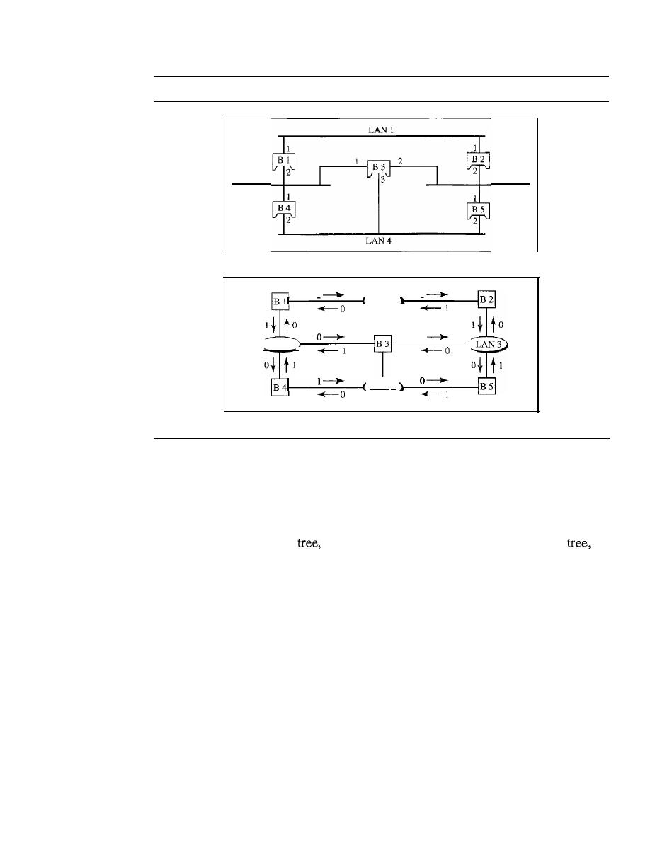
452
CHAPTER
15
CONNECTING LANs, BACKBONE NETWORKS, AND VIRTUAL LANs
Figure 15.8
A system of connected LANs and its graph representation
LAN 2
LAN 3
a. Actual system
1
!
0
LAN 1
LAN 4
LAN 2
b. Graph representation with cost assigned to each arc
2. The algorithm tries to find the shortest path (a path with the shortest cost) from the root
bridge to every other bridge or LAN. The shortest path can be found by examining the
total cost from the root bridge to the destination. Figure 15.9 shows the shortest paths.
3. The combination of the shortest paths creates the shortest tree, which is also shown
in Figure 15.9.
4. Based on the spanning
we mark the ports that are part of the spanning
the
forwarding ports, which forward a frame that the bridge receives. We also mark
those ports that are not part of the spanning tree, the blocking ports, which block
the frames received by the bridge. Figure 15.10 shows the physical systems of
LANs with forwarding points (solid lines) and blocking ports (broken lines).
Note that there is only one single path from any LAN to any other LAN in the
spanning tree system. This means there is only one single path from one LAN to any
other LAN. No loops are created. You can prove to yourself that there is only one path
from LAN 1 to LAN 2, LAN 3, or LAN 4. Similarly, there is only one path from LAN 2
to LAN 1, LAN 3, and LAN 4. The same is true for LAN 3 and LAN 4.
Dynamic Algorithm
We have described the spanning tree algorithm as though it
required manual entries. This is not true. Each bridge is equipped with a software pack-
age that carries out this process dynamically. The bridges send special messages to one
another, called bridge protocol data units (BPDUs), to update the spanning tree. The
spanning tree is updated when there is a change in the system such as a failure of a
bridge or an addition or deletion of bridges.
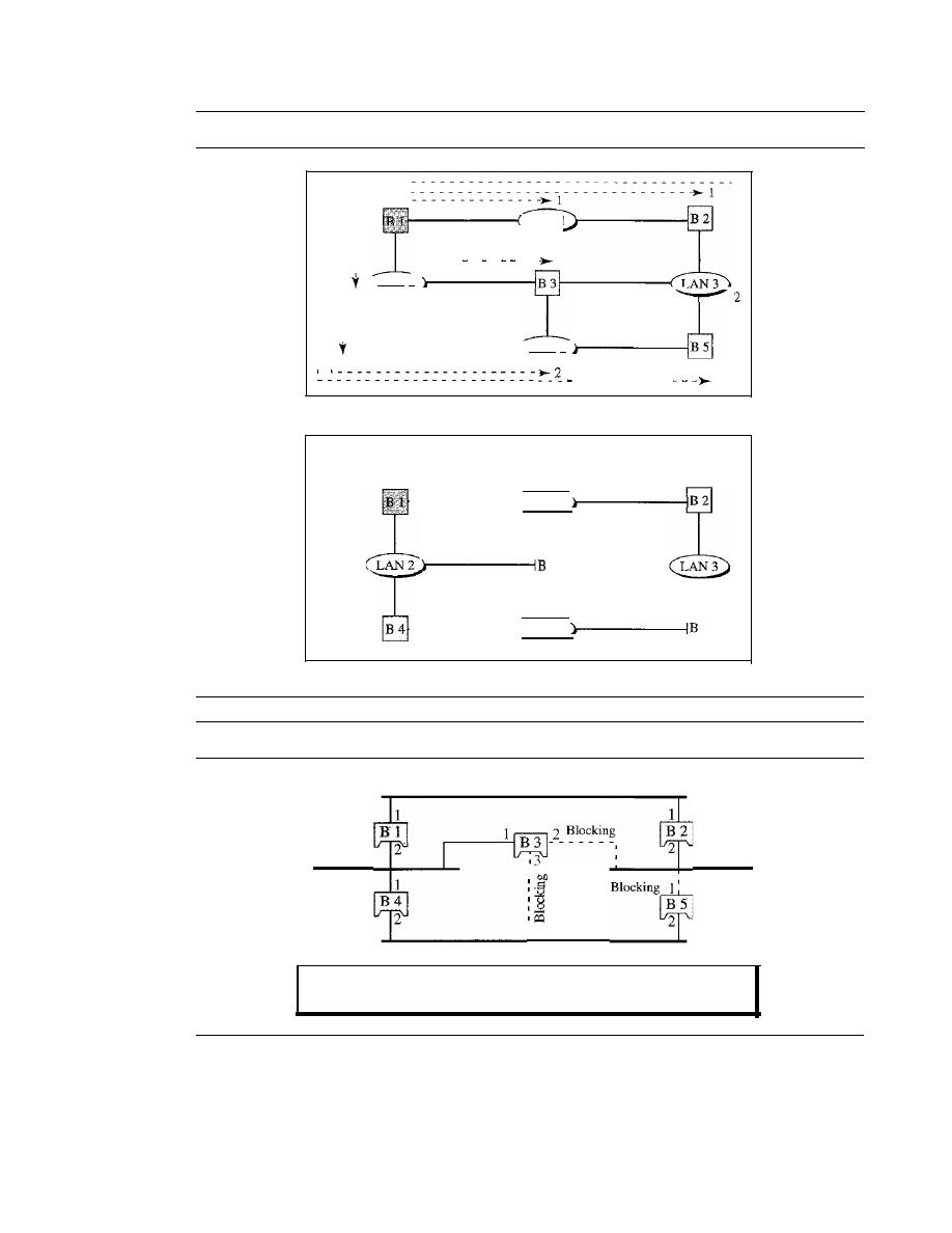
SECTION
15.1
CONNECTING DEVICES
453
Figure 15.9
Finding the shortest paths and the spanning tree in a system of bridges
,
y
'- - - - -
-
-
- -
1
LAN 1
,
,
,
,
, , :
LAN 2
I
I
1
1
, :
LAN 4
, , 1
- - - - - - - - - -
2
a. Shortest paths
Root of
spanning tree
- - - - - - ( LAN 1
3
1 - - - - - - - - (
LAN 4
5
b. Spanning tree
Figure 15.10
Forwarding and blocking ports after using spanning tree algorithm
LANl
Root bridge
LAN 2
1
1
LAN 4
LAN 3
Ports 2 and 3 of bridge B3 are blocking ports (no frame is sent out of these ports).
Port 1 of bridge B5 is also a blocking port (no frame is sent out of this port).
Source Routing Bridges
Another way to prevent loops in a system with redundant bridges is to use
source
routing
bridges.
A transparent bridge's duties include filtering frames, forwarding, and blocking.
In a system that has source routing bridges, these duties are performed
by
the source
station and, to some extent, the destination station.

454
CHAPTER
15
CONNECTING LANs, BACKBONE NE7WORKS, AND VIRTUAL LANs
In source routing, a sending station defines the bridges that the frame must visit.
The addresses of these bridges are included in the frame. In other words, the frame con-
tains not only the source and destination addresses, but also the addresses of all bridges
to be visited.
The source gets these bridge addresses through the exchange of special frames
with the destination prior to sending the data frame.
Source routing bridges were designed by IEEE to be used with Token Ring LANs.
These LANs are not very common today.
Bridges Connecting Different LANs
Theoretically a bridge should be able to connect LANs using different protocols at the
data link layer, such as an Ethernet LAN to a wireless LAN. However, there are many
issues to be considered:
o
Frame format. Each LAN type has its own frame format (compare an Ethernet
frame with a wireless LAN frame).
D
Maximum data size.
If
an incoming frame's size is too large for the destination
LAN, the data must be fragmented into several frames. The data then need to be
reassembled at the destination. However, no protocol at the data link layer allows
the fragmentation and reassembly of frames. We will see in Chapter 19 that this is
allowed in the network layer. The bridge must therefore discard any frames too
large for its system.
o
Data rate. Each LAN type has its own data rate. (Compare the 10-Mbps data rate
of an Ethernet with the I-Mbps data rate of a wireless LAN.) The bridge must
buffer the frame to compensate for this difference.
D
Bit order. Each LAN type has its own strategy in the sending of bits. Some send
the most significant bit in a byte first; others send the least significant bit first.
o
Security. Some LANs, such as wireless LANs, implement security measures in
the data link layer. Other LANs, such as Ethernet, do not. Security often involves
encryption (see Chapter 30). When a bridge receives a frame from a wireless LAN,
it needs to decrypt the message before forwarding it to an Ethernet LAN.
D
Multimedia support. Some LANs support multimedia and the quality of services
needed for this type of communication; others do not.
Two-Layer Switches
When we use the term
switch,
we must be careful because a switch can mean two dif-
ferent things. We must clarify the term by adding the level at which the device operates.
We can have a two-layer switch or a three-layer switch. A
three-layer switch is used at
the network layer; it is a kind of router. The
two-layer switch performs at the physical
and data link layers.
A two-layer switch is a bridge, a bridge with many ports and a design that allows
better (faster) performance. A bridge with a few ports can connect a few LANs
together. A bridge with many ports may be able to allocate a unique port to each station,
with each station on its own independent entity. This means no competing traffic (no
collision, as we saw in Ethernet).
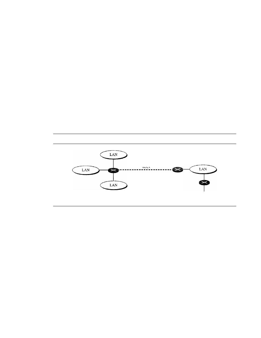
SECTION
15.1
CONNECTING DEVICES
455
A two-layer switch, as a bridge does, makes a filtering decision based on the MAC
address of the frame it received. However, a two-layer switch can be more sophisti-
cated. It can have a buffer to hold the frames for processing.
It
can have a switching fac-
tor that forwards the frames faster. Some new two-layer switches, called cut-through
switches, have been designed to forward the frame as soon as they check the MAC
addresses in the header of the frame.
Routers
A
router
is a three-layer device that routes packets based on their logical addresses
(host-to-host addressing). A router normally connects LANs and WANs in the Internet
and has a routing table that is used for making decisions about the route. The routing
tables are normally dynamic and are updated using routing protocols. We discuss rout-
ers and routing in greater detail in Chapters 19 and 21. Figure 15.11 shows a part of the
Internet that uses routers to connect LANs and WANs.
Figure 15.11
Routers connecting independent LANs and WANs
WAN
To the rest
of the Internet
Three-Layer Switches
A three-layer switch is a router, but a faster and more sophisticated. The switching fabric
in a three-layer switch allows faster table lookup and forwarding. In this book, we use
the terms router and three-layer switch interchangeably.
Gateway
Although some textbooks use the terms gateway and router interchangeably, most of the
literature distinguishes between the two. A gateway is normally a computer that operates
in all five layers of the Internet or seven layers of OSI model. A gateway takes an
application message, reads it, and interprets it. This means that it can be used as a
connecting device between two internetworks that use different models. For example,
a network designed to use the OSI model can be connected to another network using
the Internet model. The gateway connecting the two systems can take a frame as
it arrives from the first system, move it up to the OSI application layer, and remove the
message.
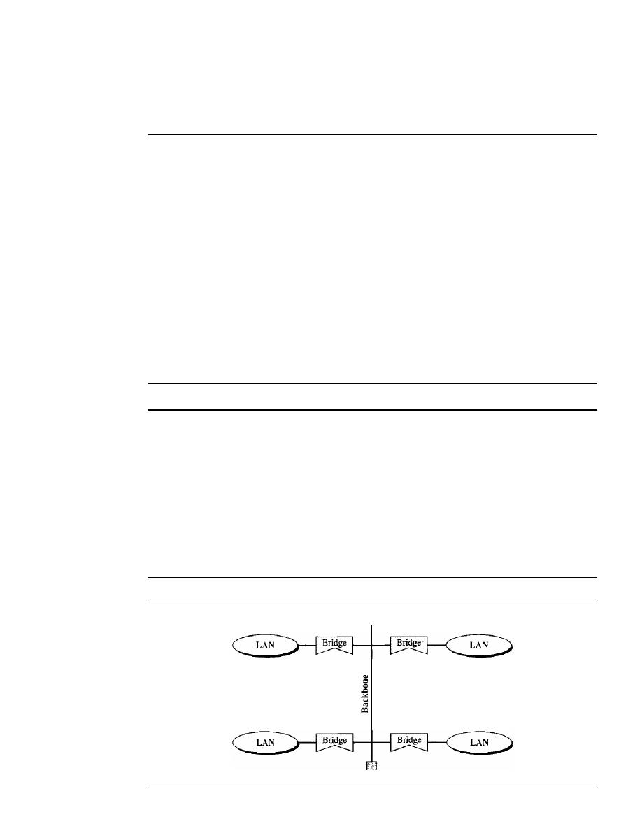
456
CHAPTER
15
CONNECTING LANs, BACKBONE NETWORKS, AND VIRTUAL LANs
Gateways can provide security. In Chapter 32, we learn that the gateway is used to
filter unwanted application-layer messages.
15.2
BACKBONE NETWORKS
Some connecting devices discussed in this chapter can be used to connect LANs in a
backbone network. A backbone network allows several LANs to be connected. In a
backbone network, no station is directly connected to the backbone; the stations are
part of a LAN, and the backbone connects the LANs. The backbone is itself a LAN
that uses a LAN protocol such as Ethernet; each connection to the backbone is itself
another LAN.
Although many different architectures can be used for a backbone, we discuss only
the two most common: the bus and the star.
Bus Backbone
In a bus
backbone, the topology of the backbone is a bus. The backbone itself can use
one of the protocols that support a bus topology such as lOBase5 or lOBase2.
In a bus backbone, the topology of the backbone is a bus.
Bus backbones are normally used as a distribution backbone to connect different
buildings in an organization. Each building can comprise either a single LAN or
another backbone (normally a star backbone). A good example of a bus backbone is
one that connects single- or multiple-floor buildings on a campus. Each single-floor
building usually has a single LAN. Each multiple-floor building has a backbone (usu-
ally a star) that connects each LAN on a floor. A bus backbone can interconnect these
LANs and backbones. Figure 15.12 shows an example of a bridge-based backbone with
four LANs.
Figure 15.12
Bus backbone
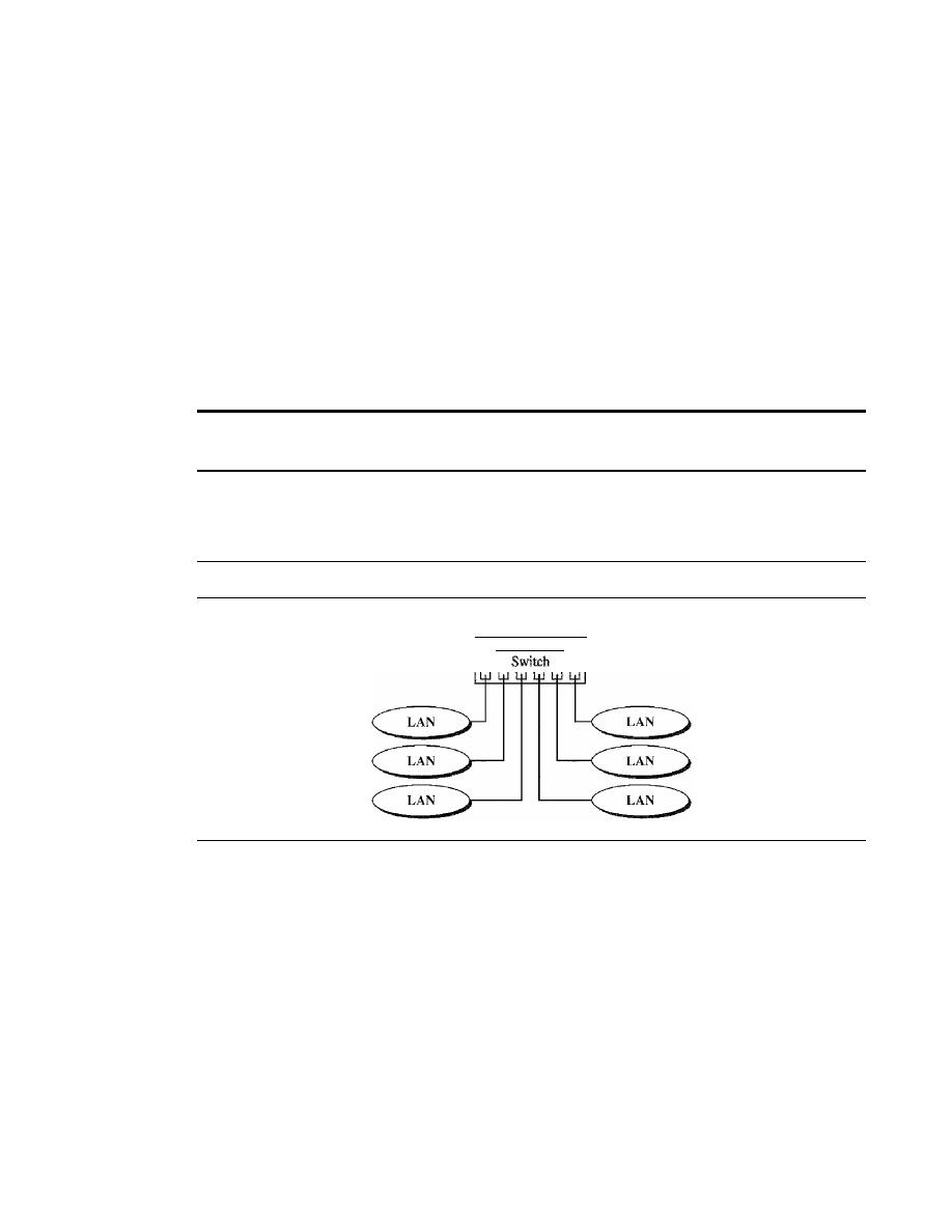
SECTION
15.2
BACKBONE NETWORKS
457
In Figure 15.12, if a station in a LAN needs to send a frame to another station in
the same LAN, the corresponding bridge blocks the frame; the frame never reaches
the backbone. However, if a station needs to send a frame to a station in another LAN, the
bridge passes the frame to the backbone, which is received by the appropriate bridge
and is delivered to the destination LAN. Each bridge connected to the backbone has a
table that shows the stations on the LAN side of the bridge. The blocking or delivery of
a frame is based on the contents of this table.
Star Backbone
In a
star backbone, sometimes called a collapsed or switched backbone, the topology
of the backbone is a star. In this configuration, the backbone is just one switch (that is
why it is called, erroneously, a collapsed backbone) that connects the LANs.
In a star backbone, the topology of the backbone is a star;
the backbone is just one switch.
Figure 15.13 shows a star backbone. Note that, in this configuration, the switch
does the job of the backbone and at the same time connects the LANs.
Figure 15.13
Star backbone
Backbone
Star backbones are mostly used as a distribution backbone inside a building. In a
multifloor building, we usually find one LAN that serves each particular floor. A star
backbone connects these LANs. The backbone network, which is just a switch, can be
installed in the basement or the first floor, and separate cables can run from the switch
to each LAN.
If
the individual LANs have a physical star topology, either the hubs (or
switches) can be installed in a closet on the corresponding floor, or all can be installed
close to the switch. We often find a rack or chassis in the basement where the backbone
switch and all hubs or switches are installed.
Connecting Remote LANs
Another common application for a backbone network is to connect remote LANs.
This type of backbone network is useful when a company has several offices with
LANs and needs to connect them. The connection can be done through bridges,
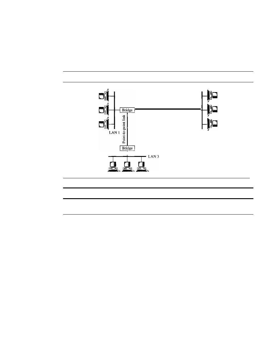
458
CHAPTER
15
CONNECTING IANs, BACKBONE NETWORKS, AND VIRTUAL IANs
sometimes called
remote bridges. The bridges act as connecting devices connecting
LANs and point-to-point networks, such as leased telephone lines or ADSL lines.
The point-to-point network in this case is considered a LAN without stations. The
point-to-point link can use a protocol such as PPP. Figure 15.14 shows a backbone
connecting remote LANs.
Figure 15.14
Connecting remote IANs with bridges
Point-to-point link
Bridge
LAN 2
A point-to-point link acts as a LAN in a remote backbone connected by remote bridges.
15.3
VIRTUAL
LANs
A station is considered part of a LAN if it physically belongs to that LAN. The criterion
of membership is geographic. What happens if we need a virtual connection between
two stations belonging to two different physical LANs? We can roughly define a
virtual
local area network (VLAN) as a local area network configured by software, not by
physical wiring.
Let us use an example to elaborate on this definition. Figure 15.15 shows a
switched LAN in an engineering firm in which 10 stations are grouped into three LANs
that are connected by a switch. The first four engineers work together as the first group,
the next three engineers work together as the second group, and the last three engineers
work together as the third group. The LAN is configured to allow this arrangement.
But what would happen if the administrators needed to move two engineers from
the first group to the third group, to speed up the project being done by the third group?
The LAN configuration would need to be changed. The network technician must
rewire. The problem is repeated if, in another week, the two engineers move back to
their previous group. In a switched LAN, changes in the work group mean physical
changes in the network configuration.
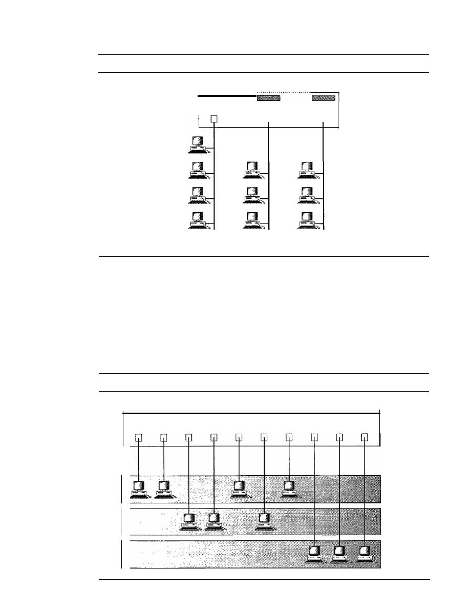
SECTION
15.3
VIRTUAL LANs
459
Figure 15.15
A switch connecting three LANs
Switch
Group
1
Group 2
Group 3
Figure 15.16 shows the same switched LAN divided into VLANs. The whole idea
of VLAN technology is to divide a LAN into logical, instead of physical, segments. A
LAN can be divided into several logical LANs called VLANs. Each VLAN is a work
group in the organization. If a person moves from one group to another, there is no need
to change the physical configuration. The group membership in VLANs is defined by
software, not hardware. Any station can be logically moved to another VLAN. All mem-
bers belonging to a VLAN can receive broadcast messages sent to that particular VLAN.
Figure 15.16
A switch using VLAN software
Switch with VLAN software
VLANI
VLAN2
VLAN3
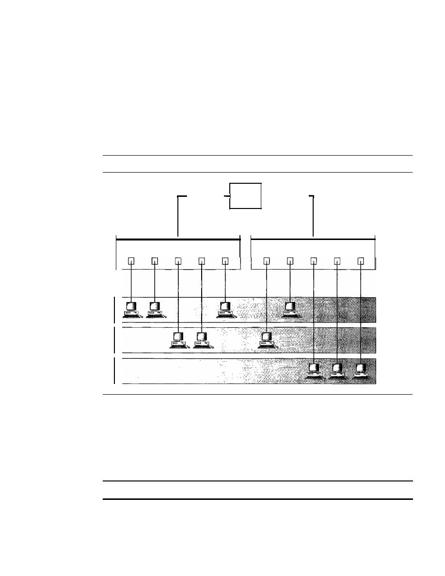
460
CHAPTER 15
CONNECTING LANs, BACKBONE NETWORKS, AND VIRTUAL LANs
This means if a station moves from VLAN 1 to VLAN 2, it receives broadcast messages
sent to VLAN 2, but no longer receives broadcast messages sent to VLAN 1.
It
is obvious that the problem in our previous example can easily be solved by
using VLANs. Moving engineers from one group to another through software is easier
than changing the configuration of the physical network.
VLAN technology even allows the grouping of stations connected to different
switches in a VLAN. Figure 15.17 shows a backbone local area network with two
switches and three VLANs. Stations from switches A and B belong to each VLAN.
Figure 15.17
Two switches in a backbone using VLAN software
Backbone
1-
switch
Switch A
Switch B
VLANI
VLAN2
VLAN3
This is a good configuration for a company with two separate buildings. Each
building can have its own switched LAN connected by a backbone. People in the first
building and people in the second building can be in the same work group even though
they are connected to different physical LANs.
From these three examples, we can define a VLAN characteristic:
VLANs create broadcast domains.
VLANs group stations belonging to one or more physical LANs into broadcast
domains. The stations in a VLAN communicate with one another as though they
belonged to a physical segment.

SECTION
15.3
VIRTUAL LANs
461
Membership
What characteristic can be used to group stations in a VLAN? Vendors use different
characteristics such as port numbers, MAC addresses, IP addresses, IP multicast
addresses, or a combination of two or more of these.
Port Numbers
Some VLAN vendors use switch port numbers as a membership characteristic. For
example, the administrator can define that stations connecting to ports 1, 2, 3, and 7
belong to VLAN 1; stations connecting to ports 4, 10, and 12 belong to VLAN 2; and
so on.
MAC Addresses
Some VLAN vendors use the 48-bit MAC address as a membership characteristic. For
example, the administrator can stipulate that stations having MAC addresses E21342A12334
and F2A123BCD34 1 belong to VLAN 1.
IP Addresses
Some VLAN vendors use the 32-bit IP address (see Chapter 19) as a membership char-
acteristic. For example, the administrator can stipulate that stations having IP addresses
181.34.23.67, 181.34.23.72, 181.34.23.98, and 181.34.23.112 belong to VLAN 1.
Multicast
IP Addresses
Some VLAN vendors use the multicast IP address (see Chapter 19) as a membership
characteristic. Multicasting at the IP layer is now translated to multicasting at the data
link layer.
Combination
Recently, the software available from some vendors allows all these characteristics to
be combined. The administrator can choose one or more characteristics when installing
the software. In addition, the software can be reconfigured to change the settings.
Configuration
How are the stations grouped into different VLANs? Stations are configured in one of
three ways: manual, semiautomatic, and automatic.
Manual Configuration
In a manual configuration, the network administrator uses the VLAN software to man-
ually assign the stations into different VLANs at setup. Later migration from one
VLAN to another is also done manually. Note that this is not a physical configuration;
it is a logical configuration. The term
manually
here means that the administrator
types the port numbers, the IP addresses, or other characteristics, using the VLAN
software.

462
CHAPTER
15
CONNECTING LANs, BACKBONE NETWORKS, AND VIRTUAL LANs
Automatic Configuration
In an automatic configuration, the stations are automatically connected or disconnected
from a VLAN using criteria defined by the administrator. For example, the administra-
tor can define the project number as the criterion for being a member of a group. When
a user changes the project, he or she automatically migrates to a new VLAN.
Semiautomatic Configuration
A semiautomatic configuration is somewhere between a manual configuration and an
automatic configuration. Usually, the initializing is done manually, with migrations
done automatically.
Communication Between Switches
In a multiswitched backbone, each switch must know not only which station belongs to
which VLAN, but also the membership of stations connected to other switches. For
example, in Figure 15.17, switch A must know the membership status of stations con-
nected to switch B, and switch B must know the same about switch
A.
Three methods
have been devised for this purpose: table maintenance, frame tagging, and time-division
multiplexing.
Table Maintenance
In this method, when a station sends a broadcast frame to its group members, the
switch creates an entry in a table and records station membership. The switches send
their tables to one another periodically for updating.
Frame Tagging
In this method, when a frame is traveling between switches, an extra header is added to
the MAC frame to define the destination VLAN. The frame tag is used by the receiving
switches to determine the VLANs to be receiving the broadcast message.
Time-Division Multiplexing (TDM)
In this method, the connection (trunk) between switches is divided into timeshared
channels (see TDM in Chapter 6). For example, if the total number of VLANs in a
backbone is five, each trunk is divided into five channels. The traffic destined for
VLAN 1 travels in channell, the traffic destined for VLAN 2 travels in channel 2, and
so on. The receiving switch determines the destination VLAN by checking the channel
from which the frame arrived.
IEEE Standard
In 1996, the IEEE 802.1 subcommittee passed a standard called 802.1 Q that defines the
format for frame tagging. The standard also defines the format to be used in multi-
switched backbones and enables the use of multivendor equipment in VLANs. IEEE
802.1 Q has opened the way for further standardization in other issues related to
VLANs. Most vendors have already accepted the standard.

SECTION 15.5
KEY7ERMS
463
Advantages
There are several advantages to using VLANs.
Cost and Time Reduction
VLANs can reduce the migration cost of stations going from one group to another.
Physical reconfiguration takes time and is costly. Instead of physically moving one sta-
tion to another segment or even to another switch, it is much easier and quicker to move
it by using software.
Creating Virtual Work Groups
VLANs can be used to create virtual work groups. For example, in a campus environ-
ment, professors working on the same project can send broadcast messages to one
another without the necessity of belonging to the same department. This can reduce
traffic if the multicasting capability of IP was previously used.
Security
VLANs provide an extra measure of security. People belonging to the same group can
send broadcast messages with the guaranteed assurance that users in other groups will
not receive these messages.
15.4
RECOMMENDED READING
For more details about subjects discussed in this chapter, we recommend the following
books and sites. The items in brackets [...] refer to the reference list at the end of the text.
Books
A book devoted to connecting devices is [PerOO]. Connecting devices and VLANs are
discussed in Section 4.7 of [Tan03]. Switches, bridges, and hubs are discussed in [Sta03]
and [Sta04].
Site
o
IEEE 802 LAN/MAN Standards Committee
15.5
KEY TERMS
amplifier
blocking port
bridge
bus backbone
connecting device
filtering
forwarding port
hub
remote bridge
repeater
router
segment

464
CHAPTER
15
CONNECTING LANs, BACKBONE NETWORKS, AND VIRTUAL LANs
source routing bridge
spanning tree
star backbone
three-layer switch
transparent bridge
two-layer switch
virtual local area network
(VLAN)
15.6
SUMMARY
o
A repeater is a connecting device that operates in the physical layer of the Internet
model. A repeater regenerates a signal, connects segments of a LAN, and has no
filtering capability.
o
A bridge is a connecting device that operates in the physical and data link layers of
the Internet model.
o
A transparent bridge can forward and filter frames and automatically build its
forwarding table.
o
A bridge can use the spanning tree algorithm to create a loopless topology.
o
A backbone LAN allows several LANs to be connected.
o
A backbone is usually a bus or a star.
o
A virtual local area network (VLAN) is configured by software, not by physical
wiring.
o
Membership in a VLAN can be based on port numbers, MAC addresses, IP
addresses, IP multicast addresses, or a combination of these features.
o
VLANs are cost- and time-efficient, can reduce network traffic, and provide an
extra measure of security.
15.7
PRACTICE SET
Review Questions
1. How is a repeater different from an amplifier?
2. What do we mean when we say that a bridge can filter traffic? Why is filtering
important?
3. What is a transparent bridge?
4. How does a repeater extend the length of a LAN?
5. How is a hub related to a repeater?
6. What is the difference between a forwarding port and a blocking port?
7. What is the difference between a bus backbone and a star backbone?
8. How does a VLAN save a company time and money?
9. How does a VLAN provide extra security for a network?
10. How does a VLAN reduce network traffic?
11. What is the basis for membership in a VLAN?

SECTION
15.7
PRACTICE SET
465
Exercises
12. Complete the table in Figure 15.6 after each station has sent a packet to another
station.
13. Find the spanning tree for the system in Figure 15.7.
14. Find the spanning tree for the system in Figure 15.8 if bridge B5 is removed.
15. Find the spanning tree for the system in Figure 15.8 if bridge B2 is removed.
16. Find the spanning tree for the system in Figure 15.8 if B5 is selected as the root
bridge.
17. In Figure 15.6, we are using a bridge. Can we replace the bridge with a router?
Explain the consequences.
18. A bridge uses a filtering table; a router uses a routing table. Can you explain the
difference?
19. Create a system of three LANs with four bridges. The bridges (B 1 to B4) connect
the LANs as follows:
a. B1 connects LAN 1 and LAN 2.
b. B2 connects LAN 1 and LAN 3.
c. B3 connects LAN 2 and LAN 3.
d. B4 connects LAN 1, LAN 2, and LAN 3.
Choose BIas the root bridge. Show the forwarding and blocking ports, after
applying the spanning tree procedure.
20. Which one has more overhead, a bridge or a router? Explain your answer.
21. Which one has more overhead, a repeater or a bridge? Explain your answer.
22. Which one has more overhead, a router or a gateway? Explain your answer.


CHAPTER 16
Wireless WANs: Cellular Telephone
and Satellite Networks
We discussed wireless LANs in Chapter 14. Wireless technology is also used in cellular
telephony and satellite networks. We discuss the former in this chapter as well as exam-
ples of channelization access methods (see Chapter 12). We also briefly discuss satellite
networks, a technology that eventually will be linked to cellular telephony to access the
Internet directly.
16.1
lELEPHONY
Cellular telephony is designed to provide communications between two moving
units, called mobile stations (MSs), or between one mobile unit and one stationary
unit, often called a land unit. A service provider must be able to locate and track a
caller, assign a channel to the call, and transfer the channel from base station to base
station as the caller moves out of range.
To make this tracking possible, each cellular service area is divided into small
regions called cells. Each cell contains an antenna and is controlled by a solar or AC
ered network station, called the base station (BS). Each base station, in tum, is controlled
by a switching office, called a mobile switching center (MSC). The MSC coordinates
communication between all the base stations and the telephone central office. It is a com-
puterized center that is responsible for connecting calls, recording call information, and
billing (see Figure 16.1).
Cell size is not fixed and can be increased or decreased depending on the popula-
tion of the area. The typical radius of a cell is 1 to 12 mi. High-density areas require
more, geographically smaller cells to meet traffic demands than do low-density areas.
Once determined, cell size is optimized to prevent the interference of adjacent cell
signals. The transmission power of each cell is kept low to prevent its signal from inter-
fering with those of other cells.
Frequency-Reuse Principle
In general, neighboring cells cannot use the same set of frequencies for communication
because it may create interference for the users located near the cell boundaries. How-
ever, the set of frequencies available is limited, and frequencies need to be reused. A
467
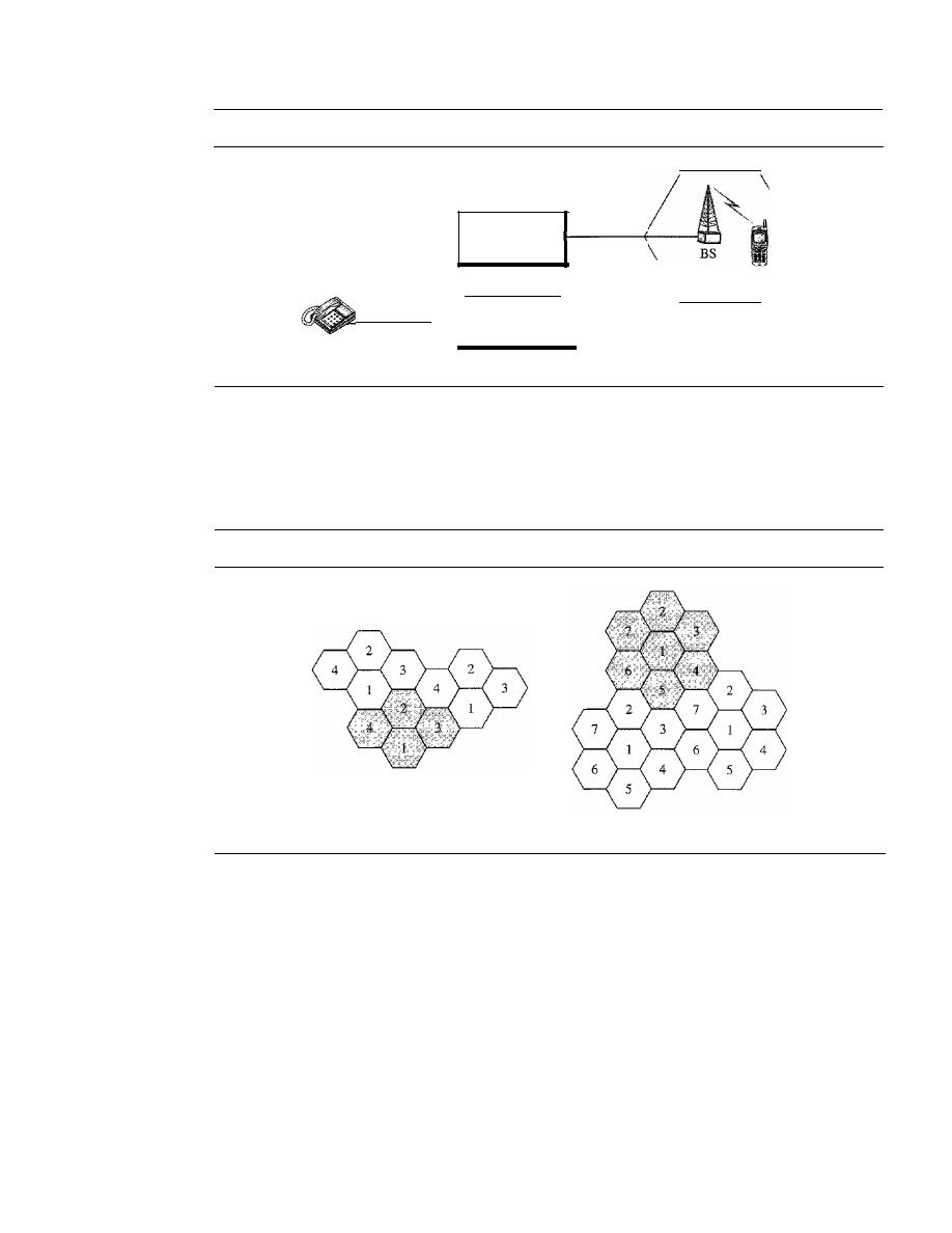
468
CHAPTER 16
WIRELESS WANs: CELLULAR TELEPHONE AND SATELLITE NETWORKS
Figure 16.1
Cellular system
Mobile switching
center
(MSC)
MS
Stationary
phone
Public switched
telephone network
(PSTN)
Cell
frequency reuse pattern is a configuration of
N
cells,
N
being the
reuse factor,
in which
each cell uses a unique set of frequencies. When the pattern is repeated, the frequencies
can be reused. There are several different patterns. Figure 16.2 shows two of them.
Figure 16.2
Frequency reuse patterns
a. Reuse factor of 4
b. Reuse factor of 7
The numbers in the cells define the pattern. The cells with the same number in a
pattern can use the same set of frequencies. We call these cells the
reusing cells.
As Fig-
ure 16.2 shows, in a pattern with reuse factor 4, only one cell separates the cells using
the same set of frequencies. In the pattern with reuse factor 7, two cells separate the
reusing cells.
Transmitting
To place a call from a mobile station, the caller enters a code of 7 or 10 digits (a phone
number) and presses the send button. The mobile station then scans the band, seeking a
setup channel with a strong signal, and sends the data (phone number) to the closest
base station using that channel. The base station relays the data to the MSC. The MSC

SECTION
16.1
CELLULAR TELEPHONY
469
sends the data on to the telephone central office.
If
the called party is available, a con-
nection is made and the result is relayed back to the MSC. At this point, the MSC
assigns an unused voice channel to the call, and a connection is established. The
mobile station automatically adjusts its tuning to the new channel, and communication
can begin.
Receiving
When a mobile phone is called, the telephone central office sends the number to the
MSC. The MSC searches for the location of the mobile station by sending query sig-
nals to each cell in a process called
paging.
Once the mobile station is found, the MSC
transmits a ringing signal and, when the mobile station answers, assigns a voice chan-
nel to the call, allowing voice communication to begin.
Handoff
It
may happen that, during a conversation, the mobile station moves from one cell to
another. When it does, the signal may become weak. To solve this problem, the MSC
monitors the level of the signal every few seconds. If the strength of the signal dimin-
ishes, the MSC seeks a new cell that can better accommodate the communication. The
MSC then changes the channel carrying the call (hands the signal off from the old
channel to a new one).
Hard Handoff
Early systems used a hard handoff. In a hard handoff, a mobile station
only communicates with one base station. When the MS moves from one cell to another,
communication must first be broken with the previous base station before communication
can be established with the new one. This may create a rough transition.
Soft Handoff
New systems use a soft handoff. In this case, a mobile station can
communicate with two base stations at the same time. This means that, during handoff,
a mobile station may continue with the new base station before breaking off from the
old one.
Roaming
One feature of cellular telephony is called roaming. Roaming means, in principle, that
a user can have access to communication or can be reached where there is coverage. A
service provider usually has limited coverage. Neighboring service providers can pro-
vide extended coverage through a roaming contract. The situation is similar to snail
mail between countries. The charge for delivery of a letter between two countries can
be divided upon agreement by the two countries.
First Generation
Cellular
is now in its second generation with the third on the horizon. The
first generation was designed for voice communication using analog signals. We discuss
one first-generation mobile system used in North America, AMPS.
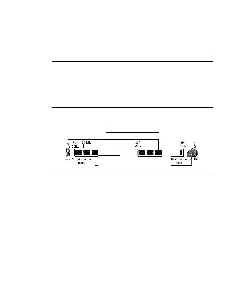
470
CHAPTER 16
WIRELESS WANs: CELLULAR TELEPHONE AND SATELLITE NETWORKS
AMPS
Advanced Mobile Phone System (AMPS) is one of the leading analog cellular sys-
tems in North America.
It
uses FDMA (see Chapter 12) to separate channels in a link.
AMPS is an analog cellular phone system using FDMA.
Bands
AMPS operates in the ISM 800-MHz band. The system uses two separate
analog channels, one for forward (base station to mobile station) communication and
one for reverse (mobile station to base station) communication. The band between 824
and 849 MHz carries reverse communication; the band between 869 and 894 MHz carries
forward communication (see Figure 16.3).
Figure 16.3
Cellular bands for AMPS
Each band is 25 MHz,
made of 832 3D-kHz analog channels
Forward communication: base to mobile
•
849
MHz
Reverse communication: mobile to base
•
Each band is divided into 832 channels. However, two providers can share an area,
which means 416 channels in each cell for each provider. Out of these 416, 21 channels
are used for control, which leaves 395 channels. AMPS has a frequency reuse factor
of 7; this means only one-seventh of these 395 traffic channels are actually available in
a cell.
Transmission
AMPS uses FM and FSK for modulation. Figure 16.4 shows the trans-
mission in the reverse direction. Voice channels are modulated using FM, and control
channels use FSK to create 30-kHz analog signals. AMPS uses FDMA to divide each
25-MHz band into 3D-kHz channels.
Second Generation
To provide higher-quality (less noise-prone) mobile voice communications, the second
generation of the cellular phone network was developed. While the first generation was
designed for analog voice communication, the second generation was mainly designed
for digitized voice. Three major systems evolved in the second generation, as shown in
Figure 16.5. We will discuss each system separately.
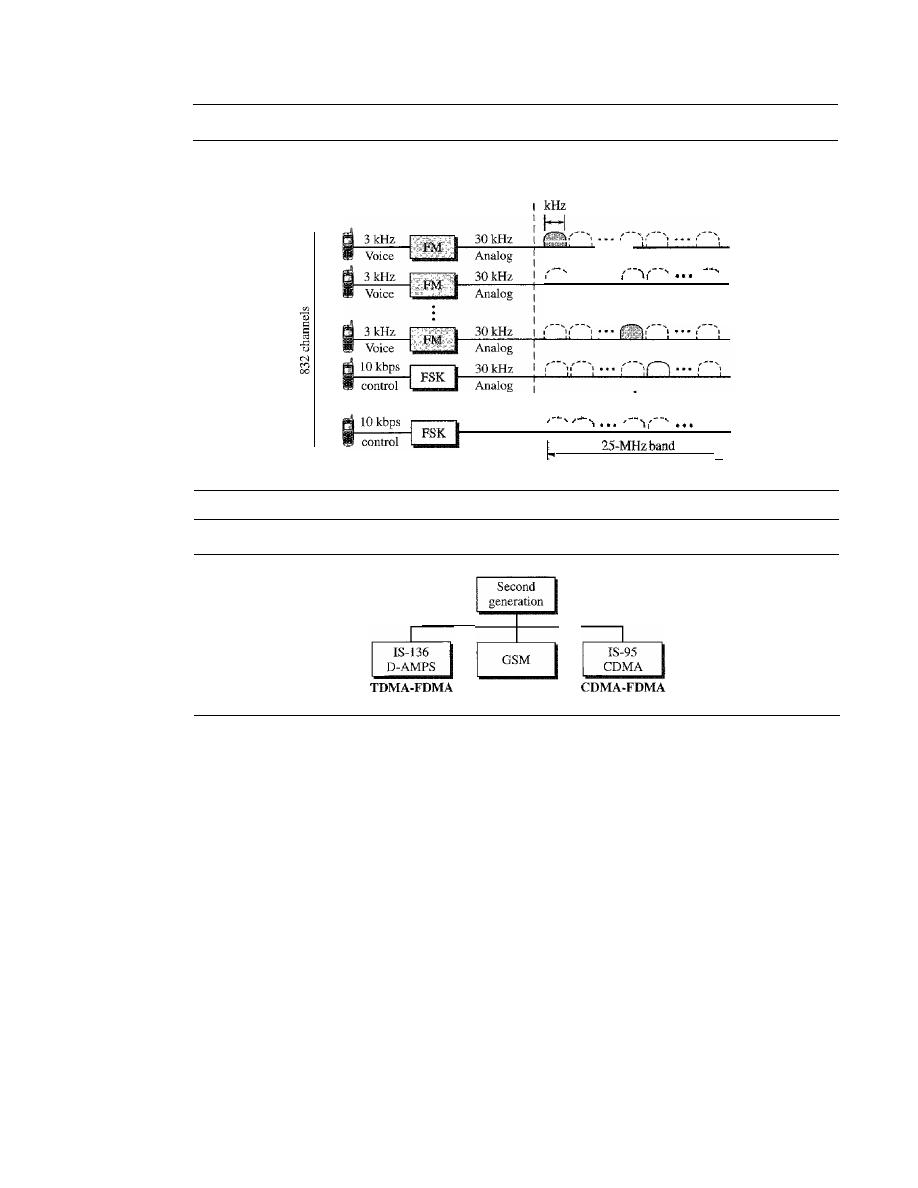
SECTION
16.1
CELLULAR TELEPHONY
471
Figure 16.4
AMPS reverse communication band
,
. . . .
1
I
\
,
FDMA
1 - - - - - - - - - - - - - - - - - 1
I
30
1
1
I
I
I
I
30kHz
Analog
I
Ii
I
I
.1
Figure 16.5
Second-generation cellular phone systems
TDMA-FDMA
D-AMPS
The product of the evolution of the analog AMPS into a digital system is
digital
AMPS
(D-AMPS). D-AMPS was designed to be backward-compatible with AMPS. This
means that in a cell, one telephone can use AMPS and another D-AMPS. D-AMPS was
first defined by IS-54 (Interim Standard 54) and later revised by IS-136.
Band
D-AMPS uses the same bands and channels as AMPS.
Transmission
Each voice channel is digitized using a very complex PCM and com-
pression technique. A voice channel is digitized to 7.95 kbps. Three 7.95-kbps digital
voice channels are combined using TDMA. The result is 48.6 kbps of digital data; much
of this is overhead. As Figure 16.6 shows, the system sends 25 frames per second, with
1944 bits per frame. Each frame lasts 40 ms (1/25) and is divided into six slots shared
by three digital channels; each channel is allotted two slots.
Each slot holds 324 bits. However, only 159 bits comes from the digitized voice;
64 bits are for control and 101 bits are for error correction. In other words, each channel
drops 159 bits of data into each of the two channels assigned to it. The system adds
64 control bits and 101 error-correcting bits.
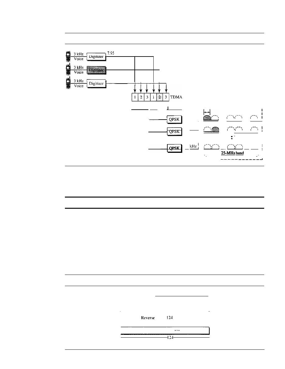
472
CHAPTER
16
WIRELESS WANs: CEllULAR TELEPHONE AND SATELLITE NETWORKS
Figure 16.6
D-AMPS
kbps
7.95 kbps
7.95 kbps
FDMA
------------------,
48.6 kbps
: 30
kHz
I
I
QPSK
30 kHz:
...
...
I
' ' ' '
" I
I
I
30 kHz:
...
...
Channel 002
.
! " !
1
I
I
I
I
I
•
I
Channel 832
30
..·
...
0
II
j
I
j
,
•
j
I
The resulting 48.6 kbps of digital data modulates a carrier using QPSK; the result
is a 3D-kHz analog signal. Finally, the 3D-kHz analog signals share a 25-MHz band
(FDMA). D-AMPS has a frequency reuse factor of 7.
D-AMPS, or 18-136, is a
digital
cellular phone system using TDMA and FDMA.
GSM
The Global System for Mobile Communication (GSM) is a European standard that
was developed to provide a common second-generation technology for all Europe. The
aim was to replace a number of incompatible first-generation technologies.
Bands
GSM uses two bands for duplex communication. Each band is 25 MHz
in width, shifted toward 900 MHz, as shown in Figure 16.7. Each band is divided into
124 channels of 200 kHz separated by guard bands.
Figure 16.7
GSM bands
Band
=
25 MHz
=
124 channels
1
1
890
band:
channels
915
MHz
MHz
935
Forward band:
channels
960
MHz
MHz
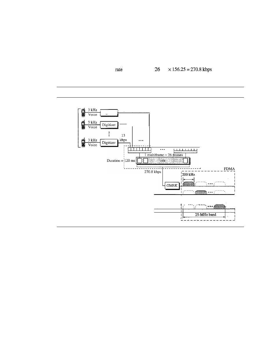
SECTION
16.1
CELLULAR TELEPHONY
473
Transmission
Figure 16.8 shows a GSM system. Each voice channel is digitized and
compressed to a 13-kbps digital signal. Each slot carries 156.25 bits (see Figure 16.9). Eight
slots share a frame (TDMA). Twenty-six frames also share a multiframe (TDMA). We
can calculate the bit rate of each channel as follows:
Channel
data
=
(11120
IDS)
x
X
8
Figure 16.8
GSM
Channel 001
8 Users
13
kbps
13
kbps
-----------------------
:
T
,
:D
I
:M
:A
Channel 002
••
Channel 124
Each 270.8-kbps digital channel modulates a carrier using GMSK (a form of
FSK used mainly in European systems); the result is a 200-kHz analog signal. Finally
124 analog channels of 200 kHz are combined using FDMA. The result is a 25-MHz
band. Figure 16.9 shows the user data and overhead in a multiframe.
The reader may have noticed the large amount of overhead in TDMA. The user
data are only 65 bits per slot. The system adds extra bits for error correction to make it
114 bits per slot. To this, control bits are added to bring it up to 156.25 bits per slot.
Eight slots are encapsulated in a frame. Twenty-four traffic frames and two additional
control frames make a multiframe. A multiframe has a duration of 120 ms. However,
the architecture does define superframes and hyperframes that do not add any overhead;
we will not discuss them here.
Reuse Factor
Because of the complex error correction mechanism, GSM allows a
reuse factor as low as 3.
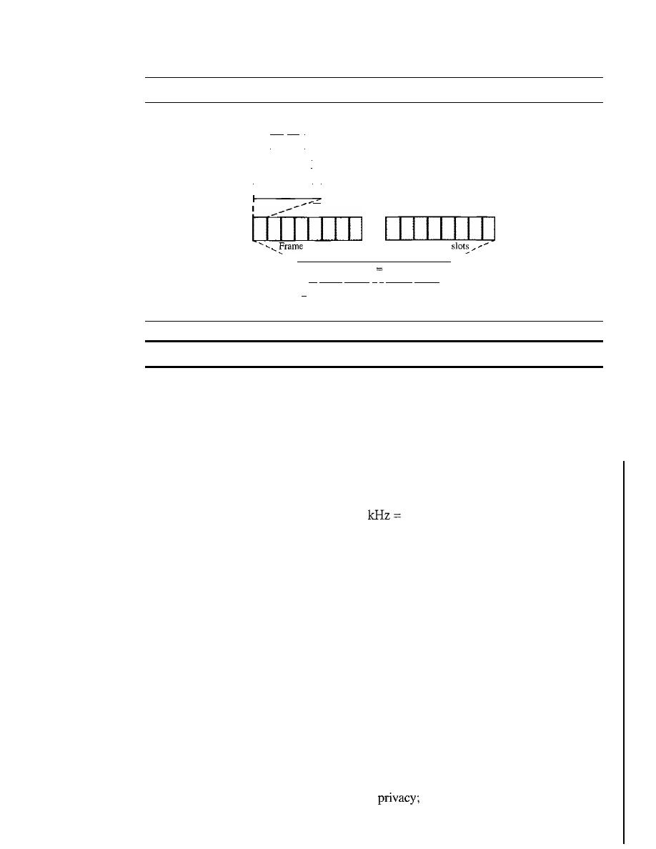
474
CHAPTER
16
WIRELESS WANs: CELLULAR TELEPHONE AND SATELLITE NETWORKS
Figure 16.9
Multiframe components
165
bits
1
User data
I
I
114 bits
I
User data plu.s
_ _ _ error control bits
I
I
I
User data plus
156.25
bits
error control bits and
TDMA control bits
...
=
8 slots
Frame
=
8
1 multiframe
26
frames
24
traffic
frames
+
2 control frames
I,
120ms
GSM is a digital cellular phone system using TDMA and FDMA.
IS-95
One of the dominant second-generation standards in North America is Interim Stan-
dard 95 (IS-95).
It
is based on CDMA and DSSS.
Bands and Channels
IS-95 uses two bands for duplex communication. The bands
can be the traditional ISM 800-MHz band or the ISM 1900-MHz band. Each band is
divided into 20 channels of 1.228 MHz separated by guard bands. Each service provider
is allotted 10 channels. IS-95 can be used in parallel with AMPS. Each IS-95 channel is
equivalent to 41 AMPS channels (41 x 30
1.23 MHz).
Synchronization
All base channels need to be synchronized to use CDMA. To pro-
vide synchronization, bases use the services of GPS (Global Positioning System), a
satellite system that we discuss in the next section.
Forward Transmission
IS-95 has two different transmission techniques: one for use
in the forward (base to mobile) direction and another for use in the reverse (mobile to
base) direction. In the forward direction, communications between the base and all
mobiles are synchronized; the base sends synchronized data to all mobiles. Figure 16.10
shows a simplified diagram for the forward direction.
Each voice channel is digitized, producing data at a basic rate of 9.6 kbps. After
adding error-correcting and repeating bits, and interleaving, the result is a signal of
19.2 ksps (kilosignals per second). This output is now scrambled using a 19.2-ksps
signal. The scrambling signal is produced from a long code generator that uses the elec-
tronic serial number (ESN) of the mobile station and generates 2
42
pseudorandom chips,
each chip having 42 bits. Note that the chips are generated pseudorandomly, not ran-
domly, because the pattern repeats itself. The output of the long code generator is fed to
a decimator, which chooses 1 bit out of 64 bits. The output of the decimator is used for
scrambling. The scrambling is used to create
the ESN is unique for each station.
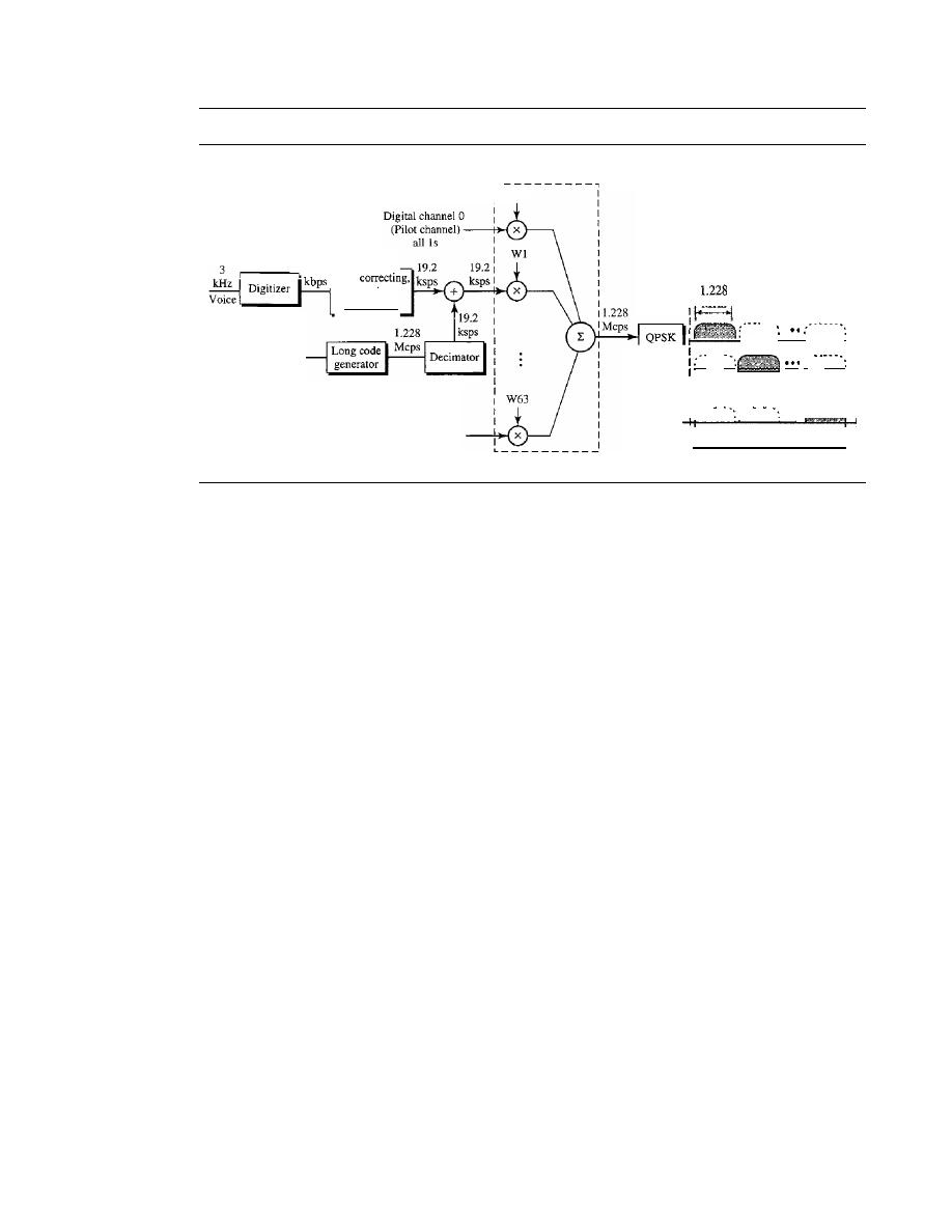
SECTION
16.1
CEILULAR TELEPHONY
475
Figure 16.10
IS-95 forward transmission
25-MHzband
FDMA
I
I
I
I
MHz
...
.
. '
•
ch'-ann-el-OZ
.....
...
:-
I
I
I
I : ••• -
: - - • .•
'+.
ChannelZO
Digital channel 63
ESN
9.6
19.Z
Error
repeatmg,
interleaving
CDMA
wo
The result of the scrambler is combined using CDMA. For each traffic channel,
one Walsh 64 x 64 row chip is selected. The result is a signal of 1.228 Mcps (megachips
per second).
19.2 ksps x 64 cps
=
1.228 Mcps
The signal is fed into a QPSK modulator to produce a signal of 1.228 MHz. The
resulting bandwidth is shifted appropriately, using FDMA. An analog channel creates
64 digital channels, of which 55 channels are traffic channels (carrying digitized voice).
Nine channels are used for control and synchronization:
o
Channel 0 is a pilot channel. This channel sends a continuous stream of 1s to mobile
stations. The stream provides bit synchronization, serves as a phase reference for
demodulation, and allows the mobile station to compare the signal strength of
neighboring bases for handoff decisions.
o
Channel 32 gives information about the system to the mobile station.
o
Channels 1 to 7 are used for paging, to send messages to one or more mobile
stations.
o
Channels 8 to 31 and 33 to 63 are traffic channels carrying digitized voice from the
base station to the corresponding mobile station.
Reverse Transmission
The use of CDMA in the forward direction is possible
because the pilot channel sends a continuous sequence of Is to synchronize transmis-
sion. The synchronization is not used in the reverse direction because we need an entity
to do that, which is not feasible. Instead of CDMA, the reverse channels use DSSS
(direct sequence spread spectrum), which we discussed
in
Chapter 8. Figure 16.11 shows
a simplified diagram for reverse transmission.
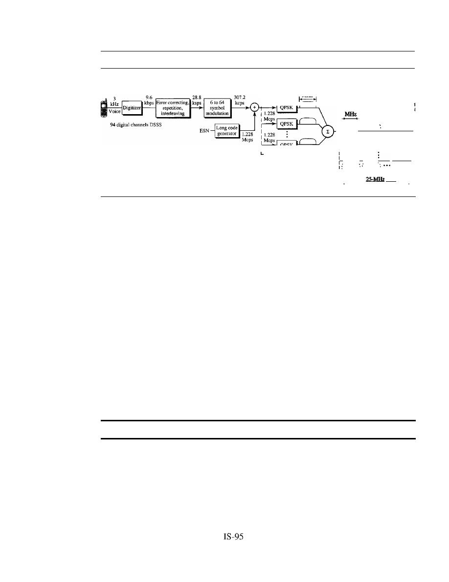
476
CHAPTER
16
WIRELESS WANs: CELLULAR TELEPHONE AND SATELliTE NETWORKS
Figure 16.11
IS-95 reverse transmission
I:
I
II
I
I
II
I
. .
!
Channel 20 :
I
I:
I
band
I
•
•
I
L
_
DSSS
r - - - - - - - - - - - - - I
I
1.228
I
I 1.228
MHz
I
FDMA
I Mcps
r - - - - - - - - - - - - - - - -
:: 1.228
I I
I
I
I
II
I
II
••• :
", :
. '
I
Each voice channel is digitized, producing data at a rate of 9.6 kbps. However,
after adding error-correcting and repeating bits, plus interleaving, the result is a signal
of 28.8 ksps. The output is now passed through a 6/64 symbol modulator. The symbols
are divided into six-symbol chunks, and each chunk is interpreted as a binary number
(from 0 to 63). The binary number is used as the index to a 64 x 64 Walsh matrix for
selection of a row of chips. Note that this procedure is not CDMA; each bit is not
multiplied by the chips in a row. Each six-symbol chunk is replaced by a 64-chip
code. This is done to provide a kind of orthogonality; it differentiates the streams of
chips from the different mobile stations. The result creates a signal of 307.2 kcps or
(28.8/6) x 64.
Spreading is the next step; each chip is spread into 4. Again the ESN of the mobile
station creates a long code of 42 bits at a rate of 1.228 Mcps, which is 4 times 307.2.
After spreading, each signal is modulated using QPSK, which is slightly different from
the one used in the forward direction; we do not go into details here. Note that there is
no multiple-access mechanism here; all reverse channels send their analog signal into
the air, but the correct chips will be received by the base station due to spreading.
Although we can create 2
42
-
1 digital channels in the reverse direction (because of
the long code generator), normally 94 channels are used; 62 are traffic channels, and
32 are channels used to gain access to the base station.
IS-95 is a digital cellular phone system using CDMAlDSSS and FDMA.
Two Data Rate Sets
IS-95 defines two data rate sets, with four different rates in each
set. The first set defines 9600, 4800, 2400, and 1200 bps.
If,
for example, the selected
rate is 1200 bps, each bit is repeated 8 times to provide a rate of 9600 bps. The second
set defines 14,400, 7200, 3600, and 1800 bps. This is possible by reducing the number
of bits used for error correction. The bit rates in a set are related to the activity of the
channel.
If
the channel is silent, only 1200 bits can be transferred, which improves the
spreading by repeating each bit 8 times.
Frequency-Reuse Factor
In an
system, the frequency-reuse factor is normally 1
because the interference from neighboring cells cannot affect CDMA or DSSS transmission.

SECTION 16.1
CELLUlAR TELEPHONY
477
Soft Handoff
Every base station continuously broadcasts signals using its pilot
channel. This means a mobile station can detect the pilot signal from its cell and neigh-
boring cells. This enables a mobile station to do a soft handoff in contrast to a hard
handoff.
pes
Before we leave the discussion of second-generation cellular telephones, let us explain
a term generally heard in relation to this generation: PCS. Personal communications
system
(peS)
does not refer to a single technology such as GSM, 18-136, or 18-95.
It
is
a generic name for a commercial system that offers several kinds of communication
services. Common features of these systems can be summarized:
1.
They may use any second-generation technology (GSM, IS-136, or IS-95).
2. They use the 1900-MHz band, which means that a mobile station needs more power
because higher frequencies have a shorter range than lower ones. However, since a
station's power is limited by the FCC, the base station and the mobile station need
to be close to each other (smaller cells).
3. They offer communication services such as short message service (SMS) and limited
Internet access.
Third Generation
The third generation of cellular telephony refers to a combination of technologies that
provide a variety of services. Ideally, when it matures, the third generation can provide
both digital data and voice communication. Using a small portable device, a person
should be able to talk to anyone else in the world with a voice quality similar to that of
the existing fixed telephone network. A person can download and watch a movie, can
download and listen to music, can surf the Internet or play games, can have a video
conference, and can do much more. One of the interesting characteristics of a third-
generation system is that the portable device is always connected; you do not need to
dial a number to connect to the Internet.
The third-generation concept started in 1992, when ITU issued a blueprint called
the Internet Mobile Communication 2000 (IMT-2000). The blueprint defines some
criteria for third-generation technology as outlined below:
o
Voice quality comparable to that of the existing public telephone network.
o
Data rate of 144 kbps for access in a moving vehicle (car), 384 kbps for access as
the user walks (pedestrians), and 2 Mbps for the stationary user (office or home).
o
Support for packet-switched and circuit-switched data services.
o
A band of 2 GHz.
o
Bandwidths of 2 MHz.
o
Interface to the Internet.
The main goal of third-generation cellular telephony is to provide
universal personal communication.
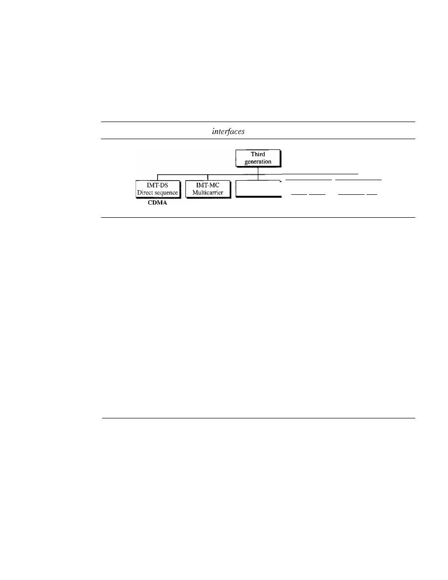
478
CHAPTER
16
WIRELESS WANs: CELLUlAR TELEPHONE AND SATELLITE NETWORKS
IMT-2000 Radio Interface
Figure 16.12 shows the radio interfaces (wireless standards) adopted by 1MT-2000. All
five are developed from second-generation technologies. The first two evolve from
COMA technology. The third evolves from a combination of COMA and TOMA. The
fourth evolves from TOMA, and the last evolves from both FOMA and TOMA.
Figure 16.12
IMT-2000 radio
IMT-SC
IMT-FT
Single carrier
Frequency time
CDMA
IMT-TC
Time code
CDMA&TDMA
TDMA
TDMA&FDMA
IMT-DS
This approach uses a version of COMA called wideband COMA or W-COMA.
W-COMA uses a 5-MHz bandwidth.
It
was developed in Europe, and it is compatible
with the COMA used in IS-95.
IMT-MC
This approach was developed in North America and is known as COMA
2000.
It
is an evolution of COMA technology used in IS-95 channels.
It
combines the
new wideband (I5-MHz) spread spectrum with the narrowband (l.25-MHz) COMA of
IS-95.
It
is backward-compatible with IS-95.
It
allows communication on multiple
1.25-MHz channels
(l,
3, 6, 9, 12 times), up to 15 MHz. The use of the wider channels
allows it to reach the 2-Mbps data rate defined for the third generation.
IMT-TC
This standard uses a combination of W-COMA and TDMA. The standard
tries to reach the IMT-2000 goals by adding TOMA multiplexing to W-COMA.
IMT-SC
This standard only uses TOMA.
IMT-FT
This standard uses a combination of FDMA and TOMA.
16.2
SATELLITE NETWORKS
A
satellite network
is a combination of nodes, some of which are satellites, that provides
communication from one point on the Earth to another. A node in the network can be a
satellite, an Earth station, or an end-user terminal or telephone. Although a natural satel-
lite, such as the Moon, can be used as a relaying node in the network, the use of artificial
satellites is preferred because we can install electronic equipment on the satellite to regen-
erate the signal that has lost its energy during travel. Another restriction on using natural
satellites is their distances from the Earth, which create a long delay in communication.
Satellite networks are like cellular networks in that they divide the planet into cells.
Satellites can provide transmission capability to and from any location on Earth, no
matter how remote. This advantage makes high-quality communication available to
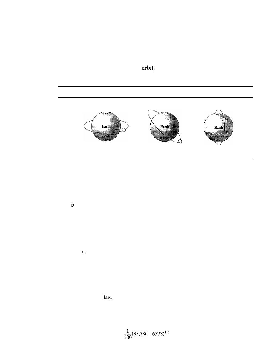
SECTION
16.2
SATELLITE NETWORKS
479
undeveloped parts of the world without requiring a huge investment in ground-based
infrastructure.
Orbits
An artificial satellite needs to have an
the path in which it travels around the Earth.
The orbit can be equatorial, inclined, or polar, as shown in Figure 16.13.
Figure 16.13
Satellite orbits
Orbit
Orbit
Orbit
a. Equatorial-orbit satellite
b. Inclined-orbit satellite
c. Polar-orbit satellite
The period of a satellite, the time required for a satellite to make a complete trip
around the Earth, is determined by Kepler's law, which defines the period as a function
of the distance of the satellite from the center of the Earth.
Example 16.1
What
the period of the Moon, according to Kepler's law?
Period:::: C
x
distance
1.5
Here C is a constant approximately equal to 1/100. The period is in seconds and the distance in
kilometers.
Solution
The Moon
located approximately 384,000 km above the Earth. The radius of the Earth is
6378 km. Applying the formula, we get
Period
=
_1_(384,000
+
6378)1.5
=
2,439,090 s
=
1 month
100
Example 16.2
According to Kepler's
what is the period of a satellite that is located at an orbit approximately
35,786
km
above the Earth?
Solution
Applying the formula, we get
Period
=
+
=
86,579 s
=
24 h
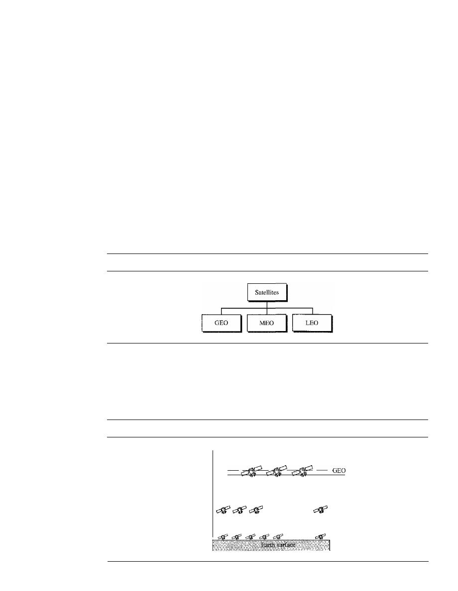
480
CHAPTER
16
WIRELESS WANs: CELLULAR TELEPHONE AND SATELLITE NETWORKS
This means that a satellite located at 35,786 km has a period of 24 h, which is the same as the
rotation period of the Earth. A satellite like this is said to be
stationary
to the Earth. The orbit, as
we will see, is called a geosynchronous orbit.
Footprint
Satellites process microwaves with bidirectional antennas (line-of-sight). Therefore, the
signal from a satellite is normally aimed at a specific area called the footprint. The sig-
nal power at the center of the footprint is maximum. The power decreases as we move
out from the footprint center. The boundary of the footprint is the location where the
power level is at a predefined threshold.
Three Categories of Satellites
Based on the location of the orbit, satellites can be divided into three categOlies: geosta-
tionary Earth orbit (GEO), low-Earth-orbit (LEO), and middle-Earth-orbit (MEO).
Figure 16.14 shows the taxonomy.
Figure 16.14
Satellite categories
Figure 16.15 shows the satellite altitudes with respect to the surface of the Earth.
There is only one orbit, at an altitude of 35,786 kIn for the OEO satellite. MEO satellites
are located at altitudes between 5000 and 15,000 kIn. LEO satellites are normally below
an altitude of 2000 km.
Figure 16.15
Satellite orbit altitudes
Altitude
(km)
35,786
Upper Van Allen belt
15,000
MEa
5000
Lower Van Allen belt
0
LEO

SECTION
16.2
SATELLITE NETWORKS
481
One reason for having different orbits is due to the existence of two Van Allen
belts. A Van Allen belt is a layer that contains charged particles. A satellite orbiting in
one of these two belts would be totally destroyed by the energetic charged particles.
The MEO orbits are located between these two belts.
Frequency Bands for Satellite Communication
The frequencies reserved for satellite microwave communication are in the gigahertz
(OHz) range. Each satellite sends and receives over two different bands. Transmission
from the Earth
to
the satellite is called the uplink. Transmission from the satellite
to
the Earth
is called the downlink. Table 16.1 gives the band names and frequencies for each range.
Table 16.1
Satellite frequency bands
Band
Downlink, GHz
Uplink, GHz
Bandwidth, MHz
L
1.5
1.6
15
S
1.9
2.2
70
C
4.0
6.0
500
Ku
11.0
14.0
500
Ka
20.0
30.0
3500
GEO Satellites
Line-of-sight propagation requires that the sending and receiving antennas be locked
onto each other's location at all times (one antenna must have the other in sight). For
this reason, a satellite that moves faster or slower than the Earth's rotation is useful
only for short periods. To ensure constant communication, the satellite must move at
the same speed as the Earth so that it seems to remain fixed above a certain spot. Such
satellites are called geostationary.
Because orbital speed is based on the distance from the planet, only one orbit can be
geostationary. This orbit occurs at the equatorial plane and is approximately 22,000 mi
from the surface of the Earth.
But one geostationary satellite cannot cover the whole Earth. One satellite in orbit
has line-of-sight contact with a vast number of stations, but the curvature of the Earth
still keeps much of the planet out of sight. It takes a minimum of three satellites equi-
distant from each other in geostationary Earth orbit (OEO) to provide full global transmis-
sion. Figure 16.16 shows three satellites, each 120° from another in geosynchronous
orbit around the equator. The view is from the North Pole.
MEO Satellites
Medium-Earth-orbit (MEO) satellites are positioned between the two Van Allen
belts. A satellite at this orbit takes approximately
6-8
hours to circle the Earth.
Global Positioning System
One example of a MEO satellite system is the Global Positioning System (GPS), con-
stracted and operated by the US Department of Defense, orbiting at an altitude about
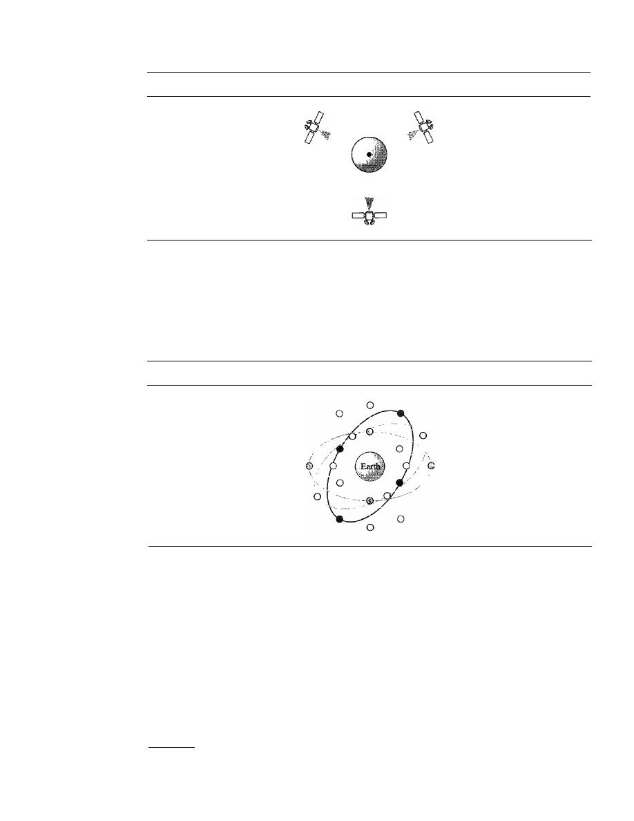
482
CHAPTER 16
WIRELESS WANs: CELLULAR TELEPHONE AND SATELLITE NETWORKS
Figure 16.16
Satellites in geostationary orbit
18,000
km (11,000
mi)
above the Earth. The system consists of 24 satellites and is used for
land, sea, and air navigation to provide time and locations for vehicles and ships. GPS
uses 24 satellites in six orbits, as shown in Figure 16.17. The orbits and the locations of
the satellites in each orbit are designed in such a way that, at any time, four satellites
are visible from any point on Earth. A GPS receiver has an almanac that tells the current
position of each satellite.
Figure 16.17
Orbits for global positioning system (GP
S)
satellites
Trilateration
GPS is based on a principle called trilateration.
t
On a plane, if we
know our distance from three points, we know exactly where we are. Let us say that we
are 10 miles away from point A, 12 miles away from point B, and 15 miles away from
point C.
If
we draw three circles with the centers at A, B, and C, we must be somewhere
on circle A, somewhere on circle B, and somewhere on circle C. These three circles meet
at one single point (if our distances are correct), our position. Figure 16.18a shows the
concept.
In three-dimensional space, the situation is different. Three spheres meet in two
points as shown in Figure 16.18b. We need at least four spheres to find our exact position
in space (longitude, latitude, and altitude). However, if we have additional facts about
our location (for example, we know that we are not inside the ocean or somewhere in
tThe tenns
trilateration
and
triangulation
are nonnally used interchangeably. We use the word
trilateration,
which means using three distances, instead of triangulation, which may mean using three angles.
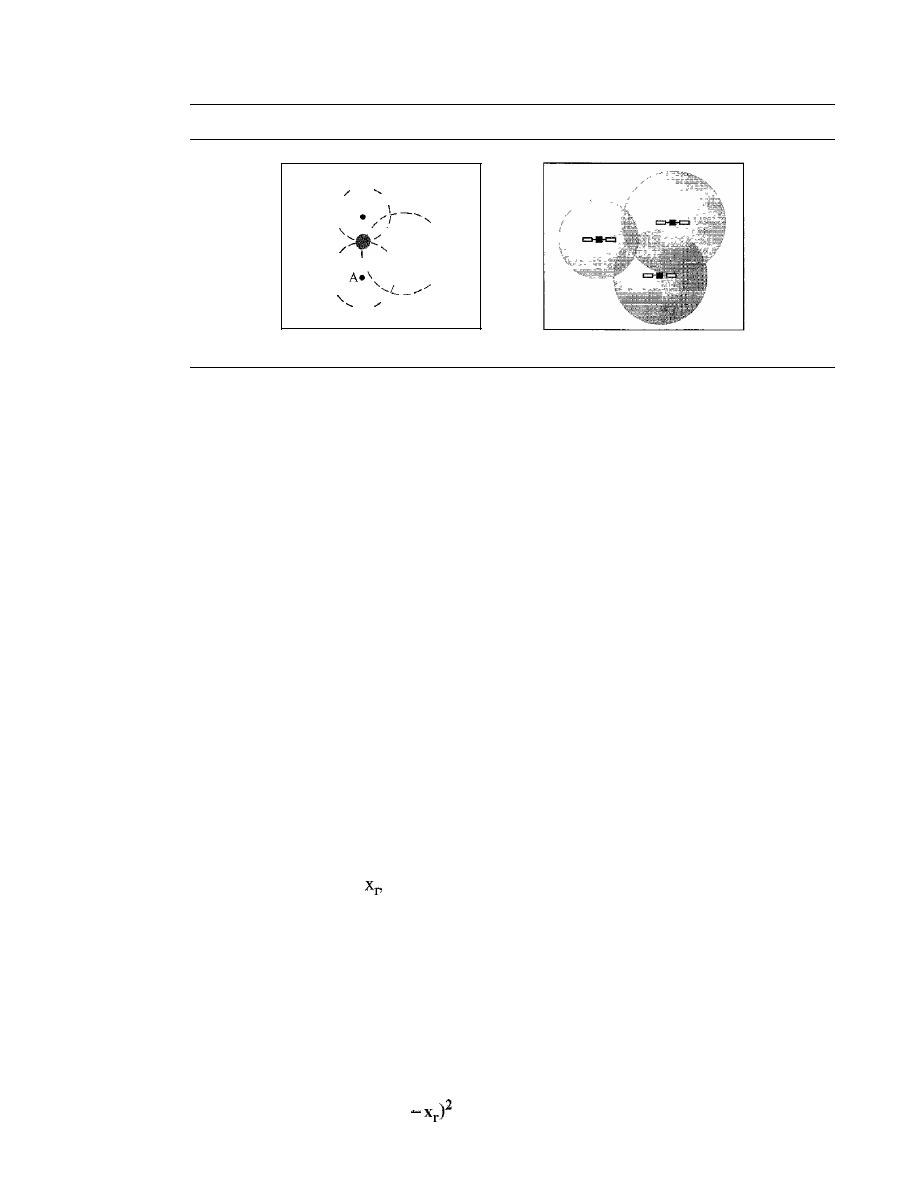
SECTION
16.2
SATELliTE NETWORKS
483
Figure 16.18
Trilateration on a plane
/
B
\
I
\
I
/
\
\
eC
\
/
\
I
I
\
\
I
\
I
/
\
/
a. Two-dimensional trilateration
b. Three-dimensional trilateration
space), three spheres are enough, because one of the two points, where the spheres meet,
is so improbable that the other can be selected without a doubt.
Measuring the Distance
The trilateration principle can find our location on the earth if
we know our distance from three satellites and know the position of each satellite. The
position of each satellite can be calculated by a GPS receiver (using the predetermined path
of the satellites). The GPS receiver, then, needs to find its distance from at least three GPS
satellites (center of the spheres). Measuring the distance is done using a principle called
one-way ranging. For the moment, let us assume that all GPS satellites and the receiver on
the Earth are synchronized. Each of 24 satellites synchronously transmits a complex signal
each having a unique pattern. The computer on the receiver measures the delay between the
signals from the satellites and its copy of signals
to
determine the distances to the satellites.
Synchronization
The previous discussion was based on the assumption that the sat-
ellites' clock are synchronized with each other and with the receiver's clock. Satellites
use atomic clock that are precise and can function synchronously with each other. The
receiver's clock however, is a normal quartz clock (an atomic clock costs more that
$50,000), and there is no way to synchronize it with the satellite clocks. There is an
unknown offset between the satellite clocks and the receiver clock that introduces a
corresponding offset in the distance calculation. Because of this offset, the measured
distance is called a pseudorange.
GPS uses an elegant solution to the clock offset problem, by recognizing that the off-
set's value is the same for all satellite being used. The calculation of position becomes find-
ing four unknowns: the
YP
zp coordinates of the receiver, and common clock offset dt.
For finding these four unknown values, we need at least four equations. This means that
we need to measure pesudoranges from four satellite instead of three.
If
we call the four
measured pseudoranges PRI, PR2, PR3 and PR4 and the coordinates of each satellite
Xi,
yj, and Zj (for i
=1
to 4), we can find the four previously mentioned unknown values
using the following four equations (the four unknown values are shown in color).
PR
I
=
[(Xl - x
r )2
+
(YI - Yr)2
+
(zl -
zr)zJlIZ
+
c X
dt
PR
z
=
[(xz -
x
r
)2
+
(yz - Yr)z
+
(zz -
zr)2JI/Z
+
ex
dt
PR
3
=
[(x3 - xr)z
+
(Y3 - Yr)z
+
(z3 - zr)ZJ1/2
+
ex
dt
PR
4
=
[(x4
+
(Y4 - Yr)z
+
(z4 - zr)ZJI/Z
+
ex
dt
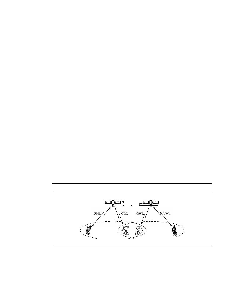
484
CHAPTER
16
WIRELESS WANs: CELLULAR TELEPHONE AND SATELLITE NETWORKS
The coordinates used in the above formulas are in an Earth-Centered Earth-Fixed
(ECEF) reference frame, which means that the origin of the coordinate space is at the
center of the Earth and the coordinate space rotate with the Earth. This implies that the
ECEF coordinates of a fixed point on the surface of the earth do not change.
Application
GPS is used by military forces. For example, thousands of portable GPS
receivers were used during the Persian Gulf war by foot soldiers, vehicles, and helicop-
ters. Another use of GPS is in navigation. The driver of a car can find the location of
the car. The driver can then consult a database in the memory of the automobile to be
directed to the destination.
In
other words, GPS gives the location of the car, and the
database uses this information to find a path to the destination. A very interesting appli-
cation is clock synchronization. As we mentioned previously, the IS-95 cellular telephone
system uses GPS to create time synchronization between the base stations.
LEO Satellites
Low-Earth-orbit (LEO) satellites have polar orbits. The altitude is between 500 and
2000 km, with a rotation period of 90 to 120 min. The satellite has a speed of 20,000 to
25,000 km/h. An LEO system usually has a cellular type of access, similar to the cellu-
lar telephone system. The footprint normally has a diameter of 8000 km. Because LEO
satellites are close to Earth, the round-trip time propagation delay is normally less than
20 ms, which is acceptable for audio communication.
An
LEO system is made of a constellation of satellites that work together as a network;
each satellite acts as a switch. Satellites that are close to each other are connected through
intersatellite links (ISLs). A mobile system communicates with the satellite through a user
mobile link (UML). A satellite can also communicate with an Earth station (gateway)
through a gateway
link
(GWL). Figure 16.19 shows a typical LEO satellite network.
Figure 16.19
LEO satellite system
ISL
I
_
Footprint
Footprint
- - - - - - - - - -
- - - - - - - - - -
LEO satellites can be divided into three categories: little LEOs, big LEOs, and broad-
band LEOs. The little LEOs operate under 1 GHz. They are mostly used for low-data-rate
messaging. The big LEOs operate between 1 and 3 GHz. Globalstar and Iridium systems
are examples of big LEOs. The broadband LEOs provide communication similar to fiber-
optic networks. The first broadband LEO system was Teledesic.
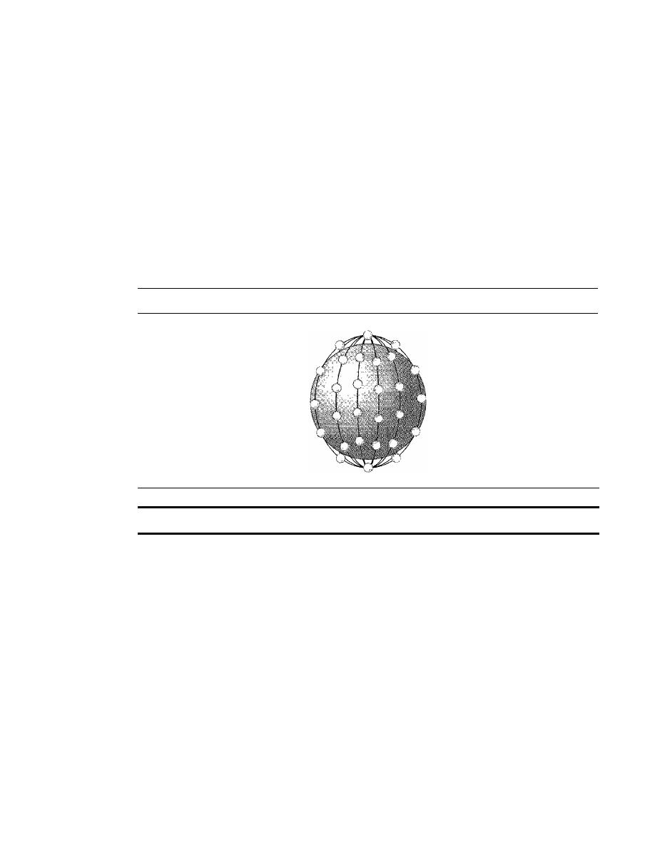
SECTION
16.2
SATELLITE NETWORKS
485
Iridium System
The concept of the
Iridium
system, a 77-satellite network, was started by Motorola in
1990. The project took eight years to materialize. During this period, the number of satel-
lites was reduced. Finally, in 1998, the service was started with 66 satellites. The original
name, Iridium, came from the name of the 77th chemical element; a mOre appropriate
name is Dysprosium (the name of element 66).
Iridium has gone through rough times. The system was halted in 1999 due to finan-
cial problems; it was sold and restarted in 2001 under new ownership.
The system has 66 satellites divided into six orbits, with 11 satellites in each orbit.
The orbits are at an altitude of 750 km. The satellites in each orbit are separated from
one another by approximately 32° of latitude. Figure 16.20 shows a schematic diagram
of the constellation.
Figure 16.20
Iridium constellation
The Iridium system has 66 satellites in six LEO orbits, each at an altitude of 750
kIn.
Since each satellite has 48 spot beams, the system can have up to 3168 beams. How-
ever, some of the beams are turned off as the satellite approaches the pole. The number of
active spot beams at any moment is approximately 2000. Each spot beam covers a cell on
Earth, which means that Earth is divided into approximately 2000 (overlapping) cells.
In the Iridium system, communication between two users takes place through satel-
lites. When a user calls another user, the call can go through several satellites before
reaching the destination. This means that relaying is done in space and each satellite
needs to be sophisticated enough to do relaying. This strategy eliminates the need for
many terrestrial stations.
The whole purpose of Iridium is to provide direct worldwide communication using
handheld terminals (same concept as cellular telephony). The system can be used for
voice, data, paging, fax, and even navigation. The system can provide connectivity
between users at locations where other types of communication are not possible. The sys-
tem provides 2.4- to 4.8-kbps voice and data transmission between portable telephones.
Transmission occurs in the 1.616- to 1.6 126-GHz frequency band. Intersatellite commu-
nication occurs in the 23.18- to 23.38-GHz frequency band.

486
CHAPTER
16
WIRELESS WANs: CELLULAR TELEPHONE AND SATELLITE NETWORKS
Iridium is designed to provide direct worldwide voice and data communication using
handheld terminals, a service similar to cellular telephony but on a global scale.
Globalstar
Globalstar is another LEO satellite system. The system uses 48 satellites in six polar
orbits with each orbit hosting eight satellites. The orbits are located at an altitude of
almost 1400 lan.
The Globalstar system is similar to the Iridium system; the main difference is the relay-
ing mechanism. Communication between two distant users in the Iridium system requires
relaying between several satellites; Globalstar communication requires both satellites and
Earth stations, which means that ground stations can create more powerful signals.
Teledesic
Teledesic is a system of satellites that provides fiber-optic-like (broadband channels,
low error rate, and low delay) communication. Its main purpose is to provide broadband
Internet access for users allover the world. It is sometimes called "Internet in the sky."
The project was started in 1990 by Craig McCaw and Bill Gates; later, other investors
joined the consortium. The project is scheduled to be fully functional in the near future.
Constellation
Teledesic provides 288 satellites in 12 polar orbits with each orbit
hosting 24 satellites. The orbits are at an altitude of 1350 lan, as shown in Figure 16.21.
Figure
16.21
Teledesic
Teledesic has 288 satellites in 12 LEO orbits, each at an altitude of 1350
kIn.
Communication
The system provides three types of communication. Intersatellite com-
munication allows eight neighboring satellites to communicate with one another. Com-
munication is also possible between a' satellite and an Earth gateway station. Users can
communicate directly with the network using terminals. Earth is divided into tens of thou-
sands of cells. Each cell is assigned a time slot, and the satellite focuses its beam to the cell

SECTION
16.5
SUMMARY
487
at the corresponding time slot. The tenninal can send data during its time slot. A tenninal
receives all packets intended for the cell, but selects only those intended for its address.
Bands
Transmission occurs in the Ka bands.
Data Rate
The data rate is up to 155 Mbps for the uplink and up to 1.2 Gbps for the
downlink.
16.3
RECOMMENDED READING
For more details about subjects discussed in this chapter, we recommend the following
books. The items in brackets [...] refer to the reference list at the end of the text.
Books
Wireless WANs are completely covered in [Sta02], [Jam03], [AZ03], and [Sch03]. Com-
munication satellites are discussed
in
Section 2.4 of [Tan03] and Section 8.5 of [CouOl].
Mobile telephone system is discussed in Section 2.6 of [Tan03] and Section 8.8 of [CouOl].
16.4
KEY TERMS
Advanced Mobile Phone System (AMPS)
cellular telephony
digital AMPS (D-AMPS)
downlink
footprint
geostationary Earth orbit (GEO)
Global Positioning System (GPS)
Global System for Mobile
Communication (GSM)
Globalstar
handoff
Interim Standard 95 (IS-95)
Internet Mobile Communication 2000
(IMT-2000)
Iridium
low-Earth-orbit (LEO)
medium-Earth-orbit (MEO)
mobile switching center (MSC)
orbit
personal communications system
(PCS)
reuse factor
roamIng
satellite network
Teledesic
triangulation
trilateration
uplink
16.5
SUMMARY
o
Cellular telephony provides communication between two devices. One or both may
be mobile.
o
A cellular service area is divided into cells.
o
Advanced Mobile Phone System (AMPS) is a first-generation cellular phone
system.

WIRELESS WANs: CELLULAR TELEPHONE AND SATELLITE NETWORKS
Digital AMPS CD-AMPS) is a second-generation cellular phone system that is a
digital version of AMPS.
Global System for Mobile Communication CGSM) is a second-generation cellular
phone system used in Europe.
Interim Standard 95 CIS-95) is a second-generation cellular phone system based on
CDMA and DSSS.
The third-generation cellular phone system will provide universal personal
communication.
A satellite network uses satellites to provide communication between any points
on Earth.
A geostationary Earth orbit CGEO) is at the equatorial plane and revolves in phase
with Earth.
Global Positioning System CGPS) satellites are medium-Earth-orbit (MEO) satellites
that provide time and location information for vehicles and ships.
Iridium satellites are low-Earth-orbit (LEO) satellites that provide direct universal
voice and data communications for handheld terminals.
Teledesic satellites are low-Earth-orbit satellites that will provide universal
broadband Internet access.
488
CHAPTER 16
0
0
0
0
0
0
0
0
0
16.6
PRACTICE SET
Review Questions
1. What is the relationship between a base station and a mobile switching center?
2. What are the functions of a mobile switching center?
3. Which is better, a low reuse factor or a high reuse factor? Explain your answer.
4. What is the difference between a hard handoff and a soft handoff?
5. What is AMPS?
6. What is the relationship between D-AMPS and AMPS?
7. What is GSM?
8. What is the function of the CDMA in IS-95?
9. What are the three types of orbits?
10. Which type of orbit does a GEO satellite have? Explain your answer.
11. What is a footprint?
12. What is the relationship between the Van Allen belts and satellites?
13. Compare an uplink with a downlink.
14. What is the purpose of GPS?
15. What is the main difference between Iridium and Globalstar?
Exercises
16. Draw a cell pattern with a frequency-reuse factor of 3.
17. What is the maximum number of callers in each cell in AMPS?

SECTION
16.6
PRACTICE SET
489
18. What is the maximum number of simultaneous calls in each cell in an 15-136
(D-AMPS) system, assuming no analog control channels?
19. What is the maximum number of simultaneous calls in each cell in a GSM assuming
no analog control channels?
20. What is the maximum number of caners in each cell in an IS-95 system?
21. Find the efficiency of AMPS in terms of simultaneous calls per megahertz of band-
width. In other words, find the number of calls that can be used in I-MHz bandwidth
allocation.
22. Repeat Exercise 21 for D-AMPS.
23. Repeat Exercise 21 for GSM.
24. Repeat Exercise 21 for IS-95.
25. Guess the relationship between a 3-kHz voice channel and a 30-kHz modulated
channel in a system using AMPS.
26. How many slots are sent each second in a channel using D-AMPS? How many slots
are sent by each user in
1
s?
27. Use Kepler's formula to check the accuracy of a given period and altitude for a
GPS satellite.
28. Use Kepler's formula to check the accuracy of a given period and altitude for an
Iridium satellite.
29. Use Kepler's formula to check the accuracy of a given period and altitude for a
Globalstar satellite.


CHAPTER 17
SONETISDH
In this chapter, we introduce a wide area network (WAN), SONET, that is used as a
transport network to carry loads from other WANs. We first discuss SONET as a protocol,
and we then show how SONET networks can be constructed from the standards defined
in the protocol.
The high bandwidths of fiber-optic cable are suitable for today's high-data-rate
technologies (such as video conferencing) and for carrying large numbers of lower-rate
technologies at the same time. For this reason, the importance of fiber optics grows in
conjunction with the development of technologies requiring high data rates or wide
bandwidths for transmission. With their prominence came a need for standardization.
The United States (ANSI) and Europe (ITU-T) have responded by defining standards
that, though independent, are fundamentally similar and ultimately compatible. The
ANSI standard is called the Synchronous Optical Network (SONET). The ITU-T
standard is called the Synchronous Digital Hierarchy (SOH).
SONET was developed by ANSI; SDH was developed by lTV·T.
SONET/SDH is a synchronous network using synchronous TDM multiplexing.
All clocks in the system are locked to a master clock.
17.1
ARCHITECTURE
Let us first introduce the architecture of a SONET system: signals, devices, and
connections.
Signals
SONET defines a hierarchy of electrical signaling levels called synchronous transport
signals (STSs). Each STS level (STS-l to STS-192) supports a certain data rate, speci-
fied in megabits per second (see Table 17.1). The corresponding optical signals are
called optical carriers (OCs). SDH specifies a similar system called a synchronous
transport module (STM). STM is intended to be compatible with existing European
491

492
CHAPTER
17
SONETISDH
hierarchies, such as E lines, and with STS levels. To this end, the lowest STM level,
STM-l, is defined as 155.520 Mbps, which is exactly equal to STS-3.
Table 17.1
SONETISDH rates
STS
OC
Rate (Mbps)
STM
STS-l
OC-l
51.840
STS-3
OC-3
155.520
STM-l
STS-9
OC-9
466.560
STM-3
STS-12
OC-12
622.080
STM-4
STS-18
OC-lS
933.120
STM-6
STS-24
OC-24
1244.160
STM-8
STS-36
OC-36
1866.230
STM-12
STS-48
OC-48
2488.320
STM-16
STS-96
OC-96
4976.640
STM-32
STS-I92
OC-I92
9953.280
STM-64
A
glance through Table 17.1 reveals some interesting points. First, the lowest level
in this hierarchy has a data rate of 51.840 Mbps, which is greater than that of the DS-3
service (44.736 Mbps). In fact, the STS-l is designed to accommodate data rates equiv-
alent to those of the DS-3. The difference in capacity is provided to handle the overhead
needs of the optical system.
Second, the STS-3 rate is exactly three times the STS-l rate; and the STS-9 rate is
exactly one-half the STS-18 rate. These relationships mean that 18 STS-l channels can
be multiplexed into one STS-18, six STS-3 channels can be multiplexed into one STS-18,
and so on.
SONET Devices
Figure 17.1 shows a simple link using SONET devices. SONET transmission relies on
three basic devices: STS multiplexers/demultiplexers, regenerators, add/drop multi-
plexers and terminals.
STS Multiplexer/Demultiplexer
STS multiplexers/demultiplexers mark the beginning points and endpoints of a SONET
link. They provide the interface between an electrical tributary network and the optical
network. An
STS multiplexer
multiplexes signals from multiple electrical sources and
creates the corresponding OC signal. An
STS demultiplexer
demultiplexes an optical
OC signal into corresponding electric signals.
Regenerator
Regenerators extend the length of the links. A regenerator is a repeater (see Chapter 15)
that takes a received optical signal
(OC-n),
demodulates it into the corresponding elec-
tric signal
(STS-n),
regenerates the electric signal, and finally modulates the electric
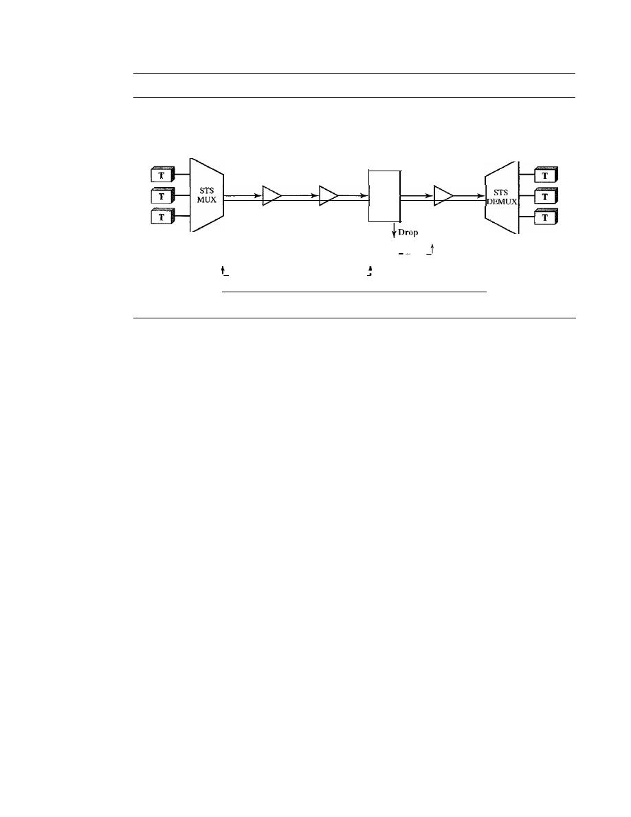
SECTION
17.1
ARCHITECTURE
493
Figure 17.1
A simple network using SONET equipment
ADM: Add/drop multiplexer
R: Regenerator
STS MUX: Synchronous transport signal multiplexer
T: Terminal
STS DEMUX: Synchronous transport signal demultiplexer
__
J
Section
Section
t
J
Line
______
_
J
Section
Section
Section
Line
R
R
R
ADM
Path
signal into its correspondent
OC-n
signal. A SONET regenerator replaces some of the
existing overhead information (header information) with new information.
Add/drop Multiplexer
Add/drop multiplexers allow insertion and extraction of signals. An
add/drop multi-
plexer (ADM) can add STSs coming from different sources into a given path or can
remove a desired signal from a path and redirect it without demultiplexing the entire
signal. Instead of relying on timing and bit positions, add/drop multiplexers use header
information such as addresses and pointers (described later in this section) to identify
individual streams.
In the simple configuration shown by Figure 17.1, a number of incoming electronic
signals are fed into an STS multiplexer, where they are combined into a single optical
signal. The optical signal is transmitted to a regenerator, where it is recreated without
the noise it has picked up in transit. The regenerated signals from a number of sources
are then fed into an add/drop multiplexer. The add/drop multiplexer reorganizes these
signals, if necessary, and sends them out as directed by information in the data frames.
These remultiplexed signals are sent to another regenerator and from there to the
receiving STS demultiplexer, where they are returned to a format usable by the receiving
links.
Terminals
A
terminal is a device that uses the services of a SONET network. For example, in the
Internet, a terminal can be a router that needs to send packets to another router at the
other side of a SONET network.
Connections
The devices defined in the previous section are connected using sections, lines, and
paths.

494
CHAPTER
17
SONETISDH
Sections
A section is the optical link connecting two neighbor devices: multiplexer to multi-
plexer, multiplexer to regenerator, or regenerator to regenerator.
Lines
A line is the portion of the network between two multiplexers: STS multiplexer to add/
drop multiplexer, two add/drop multiplexers, or two STS multiplexers.
Paths
A path is the end-to-end portion of the network between two STS multiplexers. In a
simple SONET of two STS multiplexers linked directly to each other, the section, line,
and path are the same.
17.2
SONET LAYERS
The SONET standard includes four functional layers: the photonic, the section, the
line, and the path layer. They correspond to both the physical and the data link layers
(see Figure 17.2). The headers added to the frame at the various layers are discussed
later in this chapter.
SONET defines four layers: path, line, section, and photonic.
Figure 17.2
SONET layers compared with OSI or the Internet layers
Path layer
Line layer
Data link
Physical
Section layer
Photonic layer
I
Path Layer
The path layer is responsible for the movement of a signal from its optical source to its
optical destination. At the optical source, the signal is changed from an electronic form
into an optical form, multiplexed with other signals, and encapsulated in a frame. At the
optical destination, the received frame is demultiplexed, and the individual optical sig-
nals are changed back into their electronic forms. Path layer overhead is added at this
layer. STS multiplexers provide path layer functions.
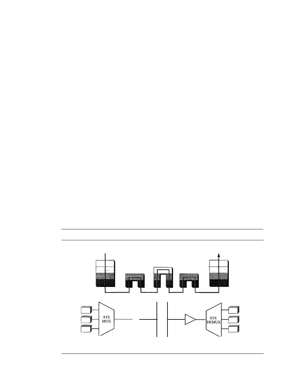
SECTION 17.2
SONET LAYERS
495
Line Layer
The
line layer
is responsible for the movement of a signal across a physical line. Line
layer overhead is added to the frame at this layer. STS multiplexers and add/drop multi-
plexers provide line layer functions.
Section Layer
The
section layer
is responsible for the movement of a signal across a physical section.
It handles framing, scrambling, and error control. Section layer overhead is added to
the frame at this layer.
Photonic Layer
The
photonic layer
corresponds to the physical layer of the OSI model. It includes
physical specifications for the optical fiber channel, the sensitivity of the receiver, mul-
tiplexing functions, and so on. SONET uses NRZ encoding with the presence of light
representing 1 and the absence of light representing O.
Device-Layer Relationships
Figure 17.3 shows the relationship between the devices used in SONET transmission
and the four layers of the standard. As you can see, an STS multiplexer is a four-layer
device. An add/drop multiplexer is a three-layer device. A regenerator is a two-layer
device.
Figure 17.3
Device-layer relationship in SONET
Electric signal
Path
Line
Section
Photonic
Optical signal
Electric signal
Path
Line
Section
Photonic
Optical signal
Optical signal
Optical signal
Regenerator
Add/drop
multiplexer
Regenerator
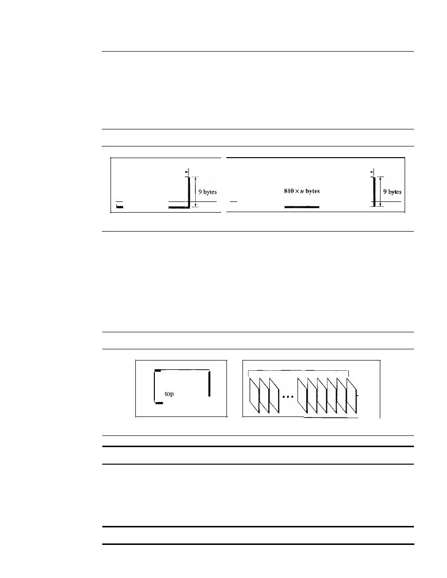
496
CHAPTER
17
SONETISDH
17.3
SONET FRAMES
Each synchronous transfer signal STS-n is composed of 8000 frames. Each frame is a
two-dimensional matrix of bytes with 9 rows by 90 x n columns. For example, STS-l
frame is 9 rows by 90 columns (810 bytes), and an STS-3 is 9 rows by 270 columns
(2430 bytes). Figure 17.4 shows the general format of an STS-l and an STS-n.
Figure 17.4
An STS-l and an STS-nframe
90 bytes
90 x
11
bytes
I ' _ _
8_10_b)_'te_s
1_'
a. STS-l frame
b. STS-n frame
Frame, Byte, and Bit Transmission
One of the interesting points about SONET is that each STS-n signal is transmitted
at a fixed rate of 8000 frames per second. This is the rate at which voice is digitized
(see Chapter 4). For each frame the bytes are transmitted from the left to the right,
top to the bottom. For each byte, the bits are transmitted from the most significant
to the least significant (left to right). Figure 17.5 shows the order of frame and
byte transmission.
Figure 17.5
STS-l frames in transition
a. Byte transmission
Left to right
and
to
bottom
First
byte
Last
byte
8000
frames/second
b. Frame transmission
A SONET
STS-n
signal is transmitted at 8000 frames per second.
If we sample a voice signal and use 8 bits
(l
byte) for each sample, we can say that
each byte in a SONET frame can carry information from a digitized voice channe1. In
other words, an STS-l signal can carry 774 voice channels simultaneously (810 minus
required bytes for overhead).
Each byte in a SONET frame can carry a digitized voice channel.
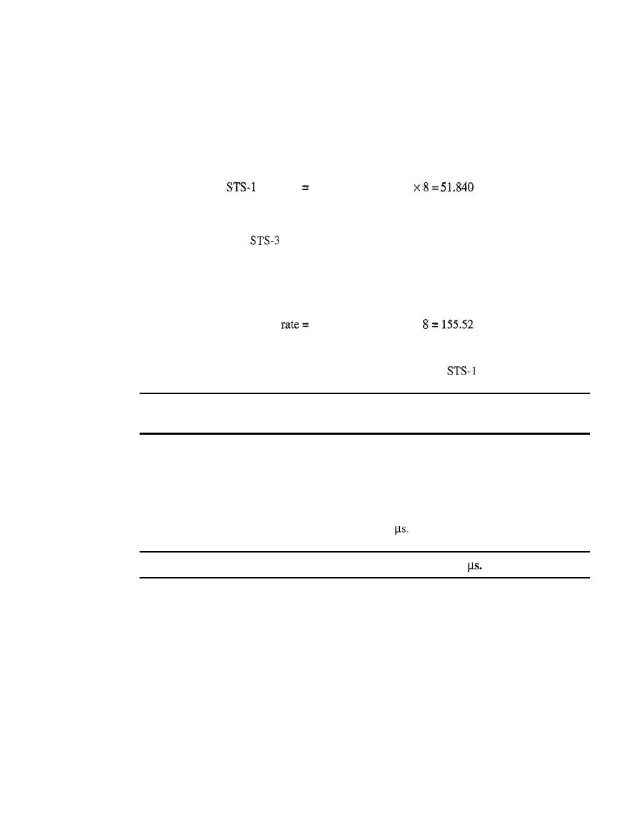
SECTION
17.3
SONET FRAMES
497
Example 17.1
Find the data rate of an STS-l signal.
Solution
STS-l, like other STS signals, sends
8000
frames per second. Each STS-l frame is made of
9
by
(l
X
90) bytes. Each byte is made of 8 bits. The data rate is
data
rate
8000
X
9
X
(1
X
90)
Mbps
Example 17.2
Find the data rate of an
signal.
Solution
STS-3, like other STS signals, sends 8000 frames per second. Each STS-3 frame is made of 9 by
(3
X
90) bytes. Each byte is made of 8 bits. The data rate is
..
.
. STS-3 data
8000 x 9 x (3
X
90)
x
Mbps
Note that in SONET, there is an exact relationship between the data rates of different STS signals.
We could have found the data rate of STS-3 by using the data rate of
(multiply the latter by 3).
In SONET, the data rate of an
STS-n
signal is
n
times the
data rate of an STS-l signals.
Example 17.3
What is the duration of an STS-l frame? STS-3 frame?
STS-n
frame?
Solution
In SONET,
8000
frames are sent per second. This means that the duration of an STS-l, STS-3, or
STS-n
frame is the same and equal to 1/8000
S,
or 125
In SONET, the duration of any frame is
125
STS-l Frame Format
The basic format of an STS-l frame is shown in Figure 17.6. As we said before, a
SONET frame is a matrix of 9 rows of 90 bytes (octets) each, for a total of 810 bytes.
The first three columns of the frame are used for section and line overhead. The
upper three rows of the first three columns are used for
section overhead (SOH). The
lower six are
line overhead (LOH). The rest of the frame is called the synchronous
payload envelope (SPE).
It
contains user data and
path overhead (POH) needed at the
user data level. We will discuss the format of the SPE shortly.
Section Overhead
The section overhead consists of nine octets. The labels, functions, and organization of
these octets are shown in Figure 17.7.
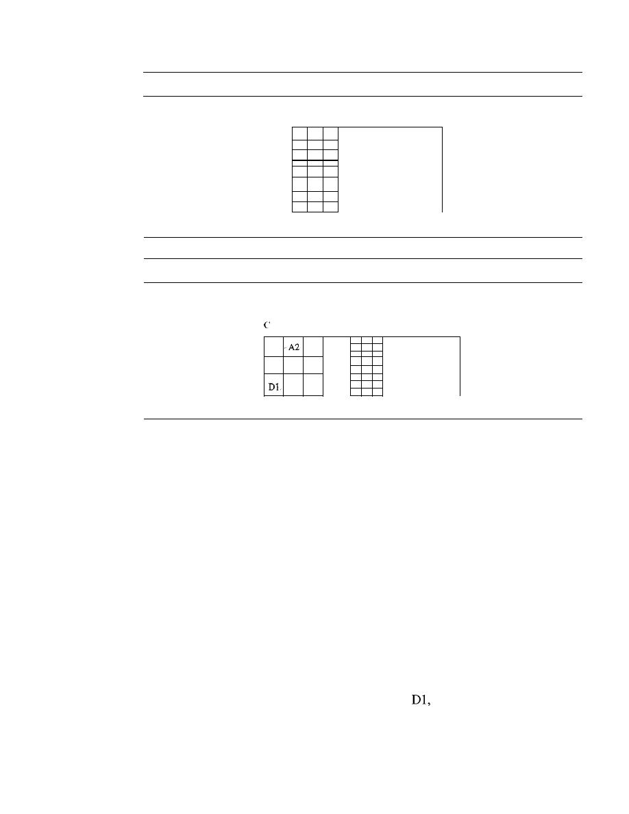
498
CHAPTER
17
SONETISDH
Figure 17.6
STS-1 frame overheads
90 octets per row
Section [
overhead
Line [
overhead
STS-I SPE
User data and
path overhead
9 rows x 87 columns
9
rows
Figure 17.7
STS-1 frame: section overhead
A I, AZ: Alignment
HI: Parity byte
1: Identification
Dl, I)Z, D3: Management
EI: Order wire byte
FI: User
Al
CI
BI
El
FI
/
STS-I SPE
D2
D3
o
Alignment bytes (AI and A2). Bytes Al and A2 are used for framing and syn-
chronization and are called alignment bytes. These bytes alert a receiver that a
frame is arriving and give the receiver a predetermined bit pattern on which to syn-
chronize. The bit patterns for these two bytes in hexadecimal are OxF628. The bytes
serve as a flag.
o
Section parity byte (BI). Byte B 1 is for bit interleaved parity (BIP-8). Its value is
calculated over all bytes of the previous frame. In other words, the ith bit of this
byte is the parity bit calculated over all ith bits of the previous STS-n frame. The
value of this byte is filled only for the first STS-l in an STS-n frame. In other
words, although an STS-n frame has n B 1 bytes, as we will see later, only the first
byte has this value; the rest are filled with Os.
o
Identification byte
(el).
Byte Cl carries the identity of the STS-l frame. This byte is
necessary when multiple STS-ls are multiplexed to create a higher-rate STS (STS-3,
STS-9, STS-12, etc.). Information in this byte allows the various signals to be recog-
nized easily upon demultiplexing. For example, in an STS-3 signal, the value of
the C1 byte is 1 for the first STS-l; it is 2 for the second; and it is 3 for the third.
o
Management bytes (DI, D2, and D3). Bytes
D2, and D3 together form a
192-kbps channel (3 x 8000 x 8) called the data communication channel. This chan-
nel is required for operation, administration, and maintenance (OA&M) signaling.
o
Order wire byte (EI). Byte El is the order wire byte. Order wire bytes in consec-
utive frames form a channel of 64 kbps (8000 frames per second times 8 bits per
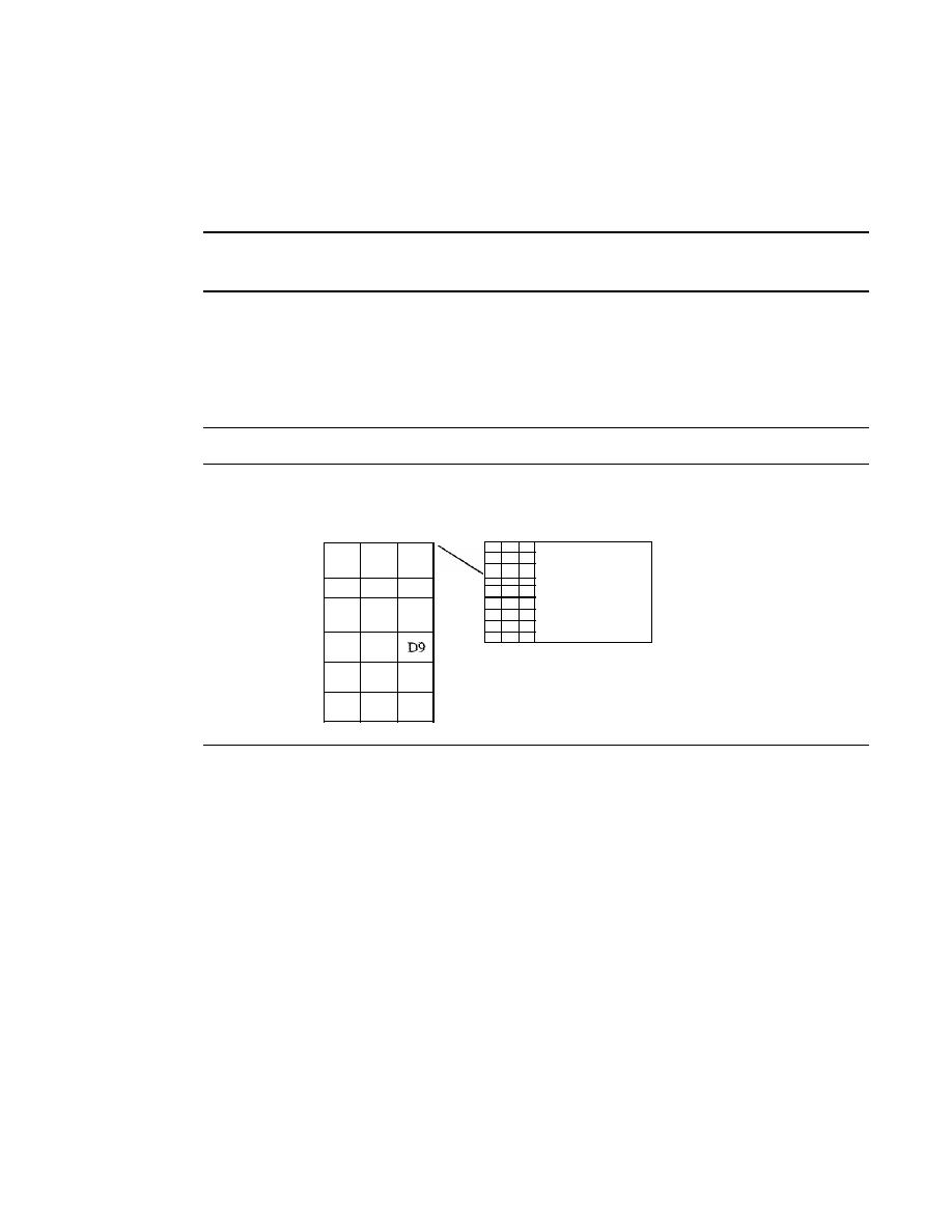
SECTION
17.3
SONET FRAMES
499
frame). This channel is used for communication between regenerators, or between
terminals and regenerators.
o
User's byte
(Fl).
The FI bytes in consecutive frames form a 64-kbps channel that
is reserved for user needs at the section level.
Section overhead is recalculated for each
SONET device
(regenerators and multiplexers).
Line Overhead
Line overhead consists of 18 bytes. The labels, functions, and arrangement of these
bytes are shown in Figure 17.8.
Figure 17.8
STS-l frame: line overhead
B2: Line parity byte
D4-DI2: Management bytes
E2: Order wire byte
HI, H2, H3: Pointers
Kl, K2: Automatic protection switching bytes
Zl, Z2: Growth bytes (reserved)
HI
HZ
H3
B2
KI
K2
STS-I SPE
D4
D5
D6
D7
08
V
DIO
Dll
DI2
Zl
Z2
E2
o
Line parity byte (B2). Byte B2 is for bit interleaved parity.
It
is for error check-
ing of the frame over a line (between two multiplexers). In an
STS-n
frame, B2 is
calculated for all bytes in the previous STS-I frame and inserted at the B2 byte
for that frame. In other words, in a STS-3 frame, there are three B2 bytes,
each calculated for one STS-I frame. Contrast this byte with B I in the section
overhead.
o
Data communication channel bytes (D4 to D12). The line overhead D bytes (D4
to D12) in consecutive frames form a 576-kbps channel that provides the same
service as the DI-D3 bytes (OA&M), but at the line rather than the section level
(between multiplexers).
o
Order wire byte (E2). The E2 bytes in consecutive frames form a 64-kbps chan-
nel that provides the same functions as the EI order wire byte, but at the line level.
o
Pointer bytes
(HI, 82, and 83). Bytes HI, H2, and H3 are pointers. The first two
bytes are used to show the offset of the SPE in the frame; the third is used for justifi-
cation. We show the use of these bytes later.
o
Automatic protection switching bytes (Kl and K2). The KI and K2 bytes in con-
secutive frames form a I28-kbps channel used for automatic detection of problems in
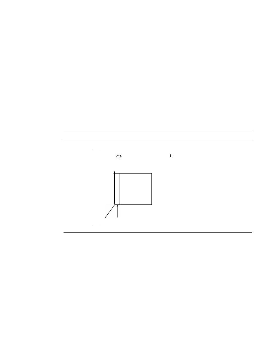
500
CHAPTER
17
SONETISDH
line-terminating equipment. We discuss automatic protection switching (APS) later
in the chapter.
D
Growth bytes (Zl and Z2). The Zl and Z2 bytes are reserved for future use.
Synchronous Payload Envelope
The
synchronous payload envelope (SPE) contains the user data and the overhead
related to the user data (path overhead). One SPE does not necessarily fit it into one STS-l
frame; it may be split between two frames, as we will see shortly. This means that the
path overhead, the leftmost column of an SPE, does not necessarily align with the
section or line overhead. The path overhead must be added first to the user data to
create an SPE, and then an SPE can be inserted into one or two frames. Path overhead
consists of 9 bytes. The labels, functions, and arrangement of these bytes are shown
in Figure 17.9.
Figure 17.9
STS-l frame: path overhead
11
B3
C2
Gl
F2
H4
B3:
Path parity byte
Path signal label byte
Gl:
Path status byte
F2: Path user channel byte
Data
H4: Virtual tributary indicator
J
Path trace byte
Z3, Z4, Z5: Growth bytes (reserved)
23
Z4
STS-I SPE
25
Path
overhead
D
Path parity byte (B3). Byte B3 is for bit interleaved parity, like bytes Bland B2,
but calculated over SPE bits.
It
is actually calculated over the previous SPE in the
stream.
D
Path signal label byte (C2). Byte C2 is the path identification byte.
It
is used to
identify different protocols used at higher levels (such as IP or ATM) whose data
are being carried in the SPE.
D
Path user channel byte (F2). The F2 bytes in consecutive frames, like the FI bytes,
form a 64-kbps channel that is reserved for user needs, but at the path level.
D
Path status byte (Gl). Byte GI is sent by the receiver to communicate its status
to the sender.
It
is sent on the reverse channel when the communication is duplex.
We will see its use in the linear or ring networks later in the chapter.
D
Multiframe indicator (H4). Byte H4 is the multiframe indicator.
It
indicates pay-
loads that cannot fit into a single frame. For example, virtual tributaries can be

SECTION 17.3
SONET FRAMES
501
combined to form a frame that is larger than an SPE frame and need to be divided
into different frames. Virtual tributaries are discussed in the next section.
o
Path trace byte (JI). The 11 bytes in consecutive frames form a 64-kbps channel
used for tracking the path. The 11 byte sends a continuous 64-byte string to verify
the connection. The choice of the string is left to the application program. The
receiver compares each pattern with the previous one to ensure nothing is wrong
with the communication at the path layer.
o
Growth bytes (Z3, Z4, and Z5). Bytes Z3, Z4, and Z5 are reserved for future use.
Path overhead is only calculated for end-to-end
(at STS multiplexers).
Overhead Summary
Table 17.2 compares and summarizes the overheads used in a section, line, and path.
Table 17.2
SONETISDH rates
Byte Function
Section
Line
Path
Alignment
Al,A2
Parity
Bl
B2
B3
Identifier
CI
C2
OA&M
DI-D3
D4-DI2
Order wire
EI
User
FI
F2
Status
Gl
Pointers
HI-H3
H4
Trace
11
Failure tolerance
KI,K2
Growth (reserved for future)
ZI, Z2
Z3-Z5
Example 17.4
What is the user data rate of an STS-l frame (without considering the overheads)?
Solution
The user data
part
in an STS-I frame is made of
9 rows and 86 columns. So we have
STS-l
data
=
86)
=
Encapsulation
The previous discussion reveals that an SPE needs to be encapsulated in an STS-I
frame. Encapsulation may create two problems that are handled elegantly by SONET
using pointers (HI to H3). We discuss the use of these bytes in this section.
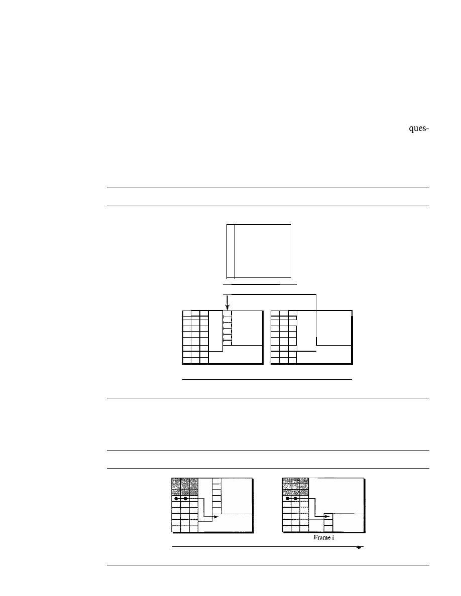
502
CHAPTER
17
SONETISDH
Offsetting
SONET allows one SPE to span two frames, part of the SPE is in the first frame and part
is in the second. This may happen when one SPE that is to be encapsulated is not aligned
time-wise with the passing synchronized frames. Figure 17.10 shows this situation. SPE
bytes are divided between the two frames. The first set of bytes is encapsulated in the
first frame; the second set is encapsulated in the second frame. The figure also shows the
path overhead, which is aligned with the section/line overhead of any frame. The
tion is, How does the SONET multiplexer know where the SPE starts or ends in the
frame? The solution is the use of pointers HI and H2 to define the beginning of the SPE;
the end can be found because each SPE has a fixed number of bytes. SONET allows the
offsetting of an SPE with respect to an STS-l frame.
Figure 17.10
Offsetting of SPE related to frame boundary
SPE
Data
I
I
I
H
Frame
1+1
Frame flow
Frame
1
To find the beginning of each SPE in a frame, we need two pointers HI and H2 in
the line overhead. Note that these pointers are located in the line overhead because the
encapsulation occurs at a multiplexer. Figure 17.11 shows how these 2 bytes point to
Figure 17.11
The use of
Hi
and H2 pointers to show the start of an SPE in aframe
Framei+l
Frame flow
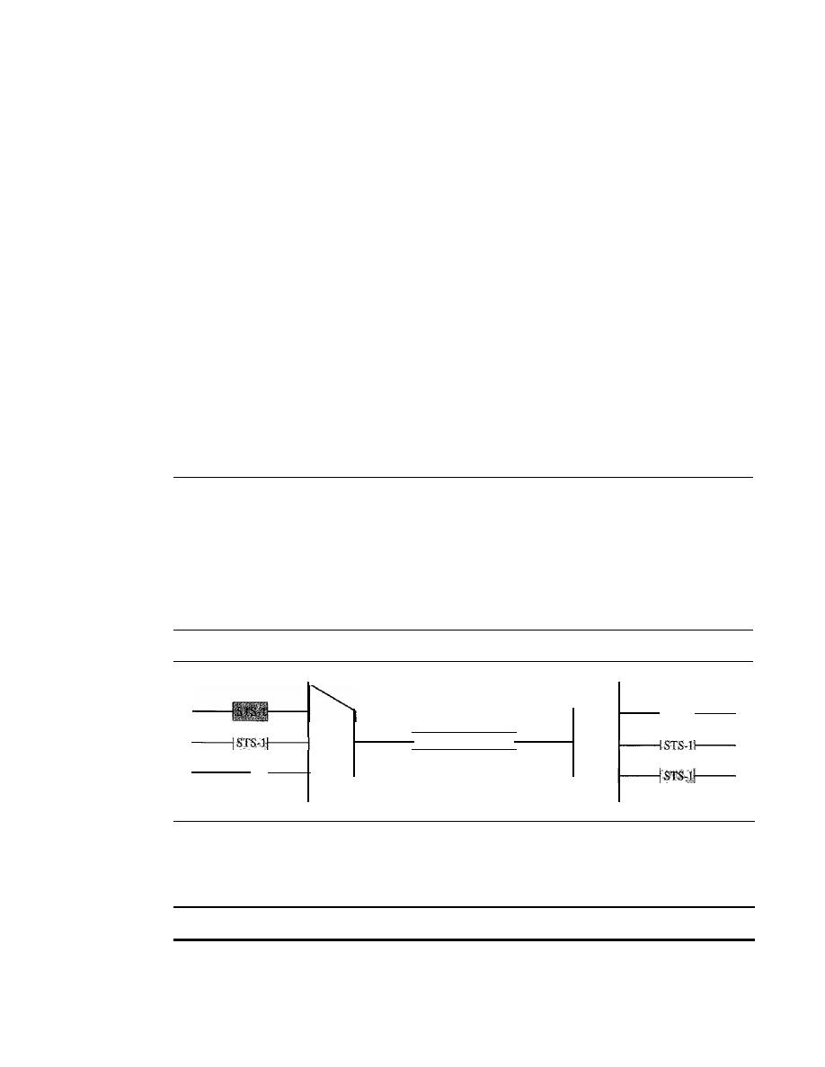
SECTION
17.4
STS MULTIPLEXING
503
the beginning of the SPEs. Note that we need 2 bytes to define the position of a byte in
a frame; a frame has 810 bytes, which cannot be defined using 1 byte.
Example 17.5
What are the values of HI and H2 if an SPE starts at byte number 650?
Solution
The number 650 can be expressed in four hexadecimal digits as Ox028A. This means the value of
HI is Ox02 and the value of H2 is Ox8A.
Justification
Now suppose the transmission rate of the payload is just slightly different from the
transmission rate of SONET. First, assume that the rate of the payload is higher. This
means that occasionally there is 1 extra byte that cannot fit in the frame. In this case,
SONET allows this extra byte to be inserted
in
the H3 byte. Now, assume that the rate of
the payload is lower. This means that occasionally 1 byte needs to be left empty in the
frame. SONET allows this byte to be the byte after the H3 byte.
17.4
STS MULTIPLEXING
In SONET, frames of lower rate can be synchronously time-division multiplexed into a
higher-rate frame. For example, three STS-l signals (channels) can be combined into
one STS-3 signal (channel), four STS-3s can be multiplexed into one STS-12, and so on,
as shown in Figure 17.12.
Figure 17.12
STS multiplexing/demultiplexing
STS
MUX
STS-3
STS
DEMUX
Multiplexing is synchronous TDM, and all clocks in the network are locked to a
master clock to achieve synchronization.
In SONET,
all
clocks in the network are locked to a master clock.
We need to mention that multiplexing can also take place at the higher data rates.
For example, four STS-3 signals can be multiplexed into an STS-12 signal. However,
the STS-3 signals need to first be demultiplexed into 12 STS-l signals, and then these
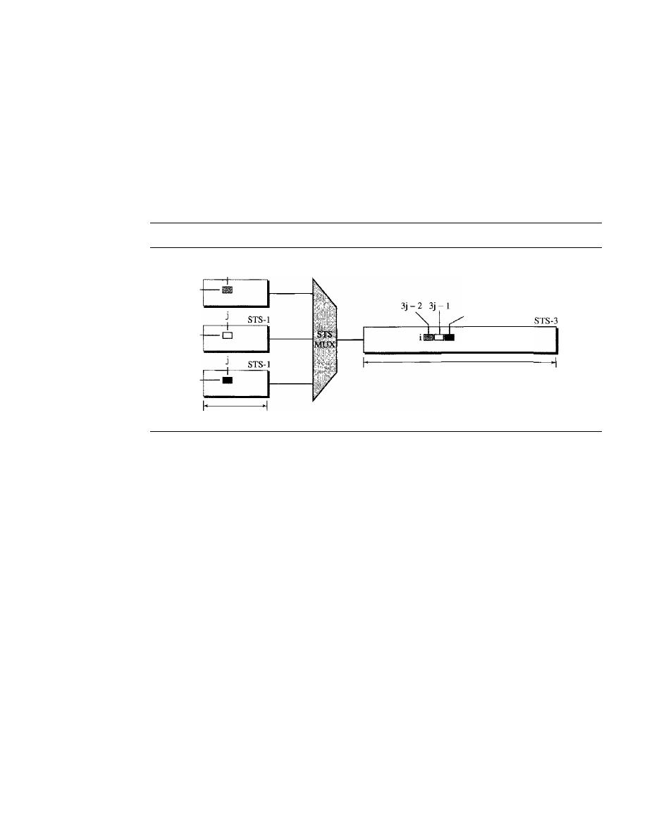
504
CHAPTER
17
SONETISDH
twelve signals need to be multiplexed into an STS-I2 signal. The reason for this extra
work will be clear after our discussion on byte interleaving.
Byte Interleaving
Synchronous TDM multiplexing in SONET is achieved by using byte interleaving.
For example, when three STS-I signals are multliplexed into one STS-3 signal, each
set of 3 bytes in the STS-3 signal is associated with 1 byte from each STS-I signal. Fig-
ure 17.13 shows the interleaving.
Figure
17.13
Byte interleaving
STS-l
90 bytes
3j
270 bytes
Note that a byte in an STS-I frame keeps its row position, but it is moved into a
different column. The reason is that while all signal frames have the same number of
rows (9), the number of columns changes. The number of columns in an STS-n signal
frame is n times the number of columns in an STS-I frame. One STS-n row, therefore,
can accommodate all
n rows in the STS-I frames.
Byte interleaving also preserves the corresponding section and line overhead as
shown in Figure 17.14. As the figure shows, the section overheads from three STS-l
frames are interleaved together to create a section overhead for an STS-l frame. The
same is true for the line overheads. Each channel, however, keeps the corresponding bytes
that are used to control that channel. In other words, the sections and lines keep their own
control bytes for each multiplexed channel. This interesting feature will allow the use of
add/drop multiplexers, as discussed shortly. As the figure shows, there are three Al bytes,
one belonging to each of the three multiplexed signals. There are also three A2 bytes,
three B 1 bytes, and so on.
Demultiplexing here is easier than in the statistical TDM we discussed in Chapter 6
because the demultiplexer, with no regard to the function of the bytes, removes the first A 1
and assigns it to the first STS-I, removes the second AI, and assigns it to second STS-l,
and removes the third Al and assigns it to the third STS-I. In other words, the demulti-
plexer deals only with the position of the byte, not its function.
What we said about the section and line overheads does not exactly apply to the path
overhead. This is because the path overhead is part of the SPE that may have splitted into
two STS-I frames. The byte interleaving, however, is the same for the data section of SPEs.
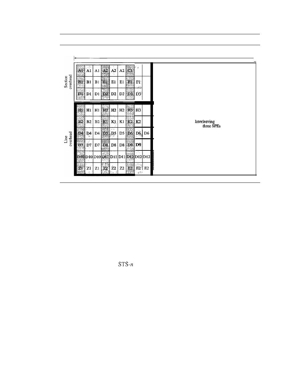
SECTION
17.4
STS MULTIPLEXING
505
Figure 17.14
AnSTS-3frame
9 bytes
Cl CI
FI
D3
H3
K2
D9
, -
261 bytes
Sr8-3SPE
bytes of
·1
The byte interleaving process makes the multiplexing at higher data rates a little
bit more complex. How can we multiplex four STS-3 signals into one STS-12 signal?
This can be done in two steps: First, the STS-3 signals must be demultiplexed to create
12 STS-l signals. The 12 STS-l signals are then multiplexed to create an STS-12 signal.
Concatenated Signal
In normal operation of the SONET, an STS-n signal is made of n multiplexed STS-l
signals. Sometimes, we have a signal with a data rate higher than what an STS-l can carry.
In this case, SONET allows us to create an STS-n signal which is not considered as n
STS-l signals; it is one
signal (channel) that cannot be demultiplexed into n
STS-l signals. To specify that the signal cannot be demultiplexed, the suffix c (for concate-
nated) is added to the name of the signal. For example, STS-3c is a signal that cannot
be demultiplexed into three STS-l signals. However, we need to know that the whole
payload in an STS-3c signal is one SPE, which means that we have only one column
(9 bytes) of path overhead. The used data in this case occupy 260 columns, as shown in
Figure 17.15.
Concatenated Signals Carrying ATM Cells
We will discuss ATM and ATM cells in Chapter 18. An ATM network is a cell network
in which each cell has a fixed size of 53 bytes. The SPE of an STS-3c signal can be a
carrier of ATM cells. The SPE of an STS-3c can carry 9 x 260
=
2340 bytes, which can
accommodate approximately 44 ATM cells, each of 53 bytes.
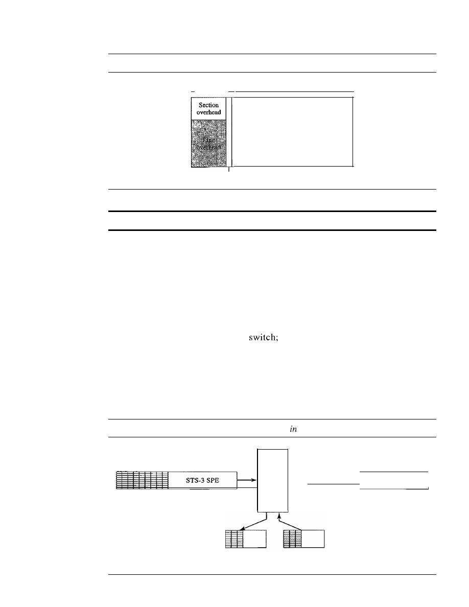
506
CHAPTER
17
SONETISDH
Figure 17.15
A concatenated STS-3c signal
I_
10 octets
_I_
Path overhead
260 octets
STS-3cSPE
An STS-3c signal can carry 44 ATM cells as its SPE.
AddlDrop Multiplexer
Multiplexing of several STS-1 signals into an STS-n signal is done at the STS multi-
plexer (at the path layer). Demultiplexing of an STS-n signal into STS-1 components
is done at the STS demultiplexer. In between, however, SONET uses add/drop multi-
plexers that can replace a signal with another one. We need to know that this is not
demultiplexing/multiplexing in the conventional sense. An add/drop multiplexer
operates at the line layer. An add/drop multiplexer does not create section, line, or
path overhead. It almost acts as a
it removes one STS-1 signal and adds
another one. The type of signal at the input and output of an add/drop multiplexer is
the same (both STS-3 or both STS-12, for example). The add/drop multiplexer
(ADM) only removes the corresponding bytes and replaces them with the new bytes
(including the bytes in the section and line overhead). Figure 17.16 shows the opera-
tion of an ADM.
Figure 17.16
Dropping and adding STS-l frames
an add/drop multiplexer
ADM
_
STS-3SPE
Third STS-l
is
dropped
New
STS-l
is
added
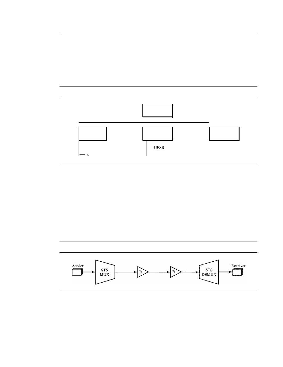
SECTION
17.5
SONET NETWORKS
507
17.5
SONET NETWORKS
Using SONET equipment, we can create a SONET network that can be used as a high-speed
backbone carrying loads from other networks such as ATM (Chapter 18) or IF (Chapter 20).
We can roughly divide SONET networks into three categories: linear, ring, and mesh net-
works, as shown in Figure 17.17.
Figure
17.17
Taxonomy of
so
NET networks
BLSR
!\
Inltlpomt
SONET
networks
I
I
I
I
Linear
Ring
Mesh
networks
networks
networks
-
Point-to-point
-
-
Linear
Networks
A linear SONET network can be point-to-point or multipoint.
Point-to-Point Network
A point-to-point network is normally made of an STS multiplexer, an STS demultiplexer,
and zero or more regenerators with no add/drop multiplexers, as shown in Figure 17.18.
The signal flow can be unidirectional or bidirectional, although Figure 17.18 shows
only unidirectional for simplicity.
Figure
17.18
A point-to-point SONET network
,'.
Multipoint Network
A multipoint network uses ADMs to allow the communications between several termi-
nals. An ADM removes the signal belonging to the terminal connected to it and adds
the signal transmitted from another terminal. Each terminal can send data to one or more
downstream terminals. Figure 17.19 shows a unidirectional scheme in which each ter-
minal can send data only to the downstream terminals, but the a multipoint network can
be bidirectional, too.
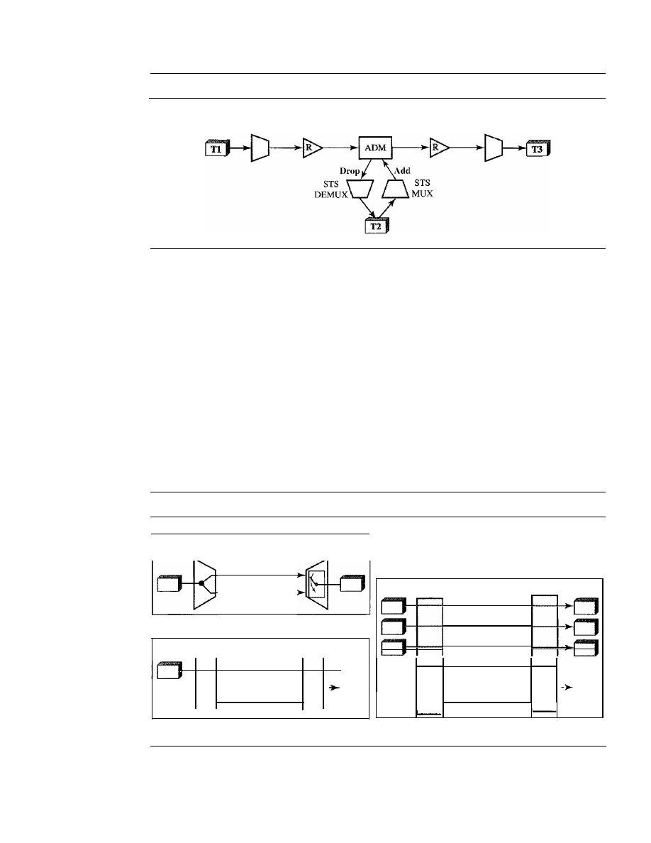
50S
CHAPTER
17
SONETISDH
Figure 17.19
A multipoint SONET network
STS
MUX
STS
DEMUX
In Figure 17.19, Tl can send data to T2 and T3 simultaneously. T2, however, can
send data only to T3. The figure shows a very simple configuration; in normal situa-
tions, we have moreADMs and more terminals.
Automatic Protection Switching
To create protection against failure in linear networks, SONET defines automatic pro-
tection switching (APS).
APS in linear networks is defined at the line layer, which
means the protection is between two ADMs or a pair of STS multiplexer/demultiplexers.
The idea is to provide redundancy; a redundant line (fiber) can be used in case of failure
in the main one. The main line is referred to as the work line and the redundant line
as the protection line. Three schemes are common for protection in linear channels:
one-plus-one, one-to-one, and one-to-many. Figure 17.20 shows all three schemes.
Figure 17.20
Automatic protection switching in linear networks
-----------
--
STS
MUX
a. One-pIus-one APS
ADM
b. One-to-one APS
Working line
Protection line
Working line
Protection line
Reverse line
STS
MUX
ADM
ADM
ADM
Working lines
0
Protection line
-
-
- --
-------------
-
--
Reverse line
c. One-to-many APS
One-Plus-One APS
In this scheme, there are normally two lines: one working line
and one protection line. Both lines are active all the time. The sending multiplexer

SECTION 17.5
SONET NETWORKS
509
sends the same data on both lines; the receiver multiplexer monitors the line and
chooses the one with the better quality.
If
one of the lines fails, it loses its signal, and, of
course, the other line is selected at the receiver. Although, the failure recovery for this
scheme is instantaneous, the scheme is inefficient because two times the bandwidth is
required. Note that one-plus-one switching is done at the path layer.
One-to-One APS
In this scheme, which looks like the one-plus-one scheme, there is
also one working line and one protection line. However, the data are normally sent on
the working line until it fails. At this time, the receiver, using the reverse channel,
informs the sender to use the protection line instead. Obviously, the failure recovery is
slower than that of the one-plus-scheme, but this scheme is more efficient because the
protection line can be used for data transfer when it is not used to replace the working
line. Note that the one-to-one switching is done at the line layer.
One-to-Many APS
This scheme is similar to the one-to-one scheme except that
there is only one protection line for many working lines. When a failure occurs in one
of the working lines, the protection line takes control until the failed line is repaired. It
is not as secure as the one-to-one scheme because if more than one working line fails at
the same time, the protection line can replace only one of them. Note that one-to-many
APS is done at the line layer.
Ring Networks
ADMs make it possible to have SONET ring networks. SONET rings can be used in
either a unidirectional or a bidirectional configuration. In each case, we can add extra
rings to make the network self-healing, capable of self-recovery from line failure.
Unidirectional Path Switching Ring
A unidirectional path switching ring (UPSR) is a unidirectional network with two
rings: one ring used as the working ring and the other as the protection ring. The idea is
similar to the one-plus-one APS scheme we discussed in a linear network. The same
signal flows through both rings, one clockwise and the other counterclockwise.
It
is
called
because monitoring is done at the path layer. A node receives two copies
of the electrical signals at the path layer, compares them, and chooses the one with the
better quality. If part of a ring between two ADMs fails, the other ring still can guaran-
tee the continuation of data flow. UPSR, like the one-plus-one scheme, has fast failure
recovery, but it is not efficient because we need to have two rings that do the job of one.
Half of the bandwidth is wasted. Figure 17.21 shows a UPSR network.
Although we have chosen one sender and three receivers in the figure, there can be
many other configurations. The sender uses a two-way connection to send data to both
rings simultaneously; the receiver uses selecting switches to select the ring with better
signal quality. We have used one STS multiplexer and three STS demultiplexers to
emphasize that nodes operate on the path layer.
Bidirectional Line Switching Ring
Another alternative in a SONET ring network is bidirectional line switching ring
(BLSR). In this case, communication is bidirectional, which means that we need
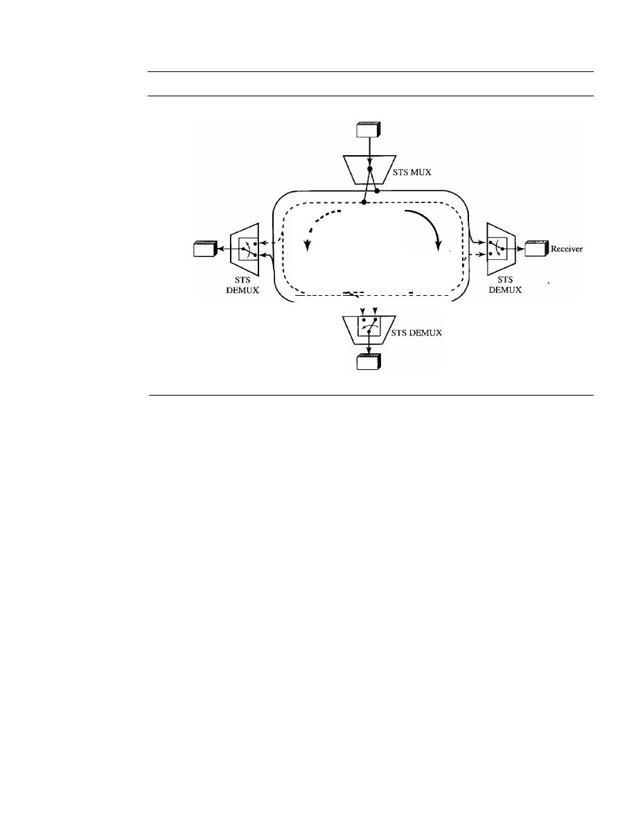
510
CHAPTER
17
SONETISDH
Figure 17.21
A unidirectional path switching ring
Sender
--
-
--
-
- - - - - -
-
- - -
...
Receiver
;
,
Protection
ring
Working
ring
I
Receiver
two rings for working lines. We also need two rings for protection lines. This means
BLSR uses four rings. The operation, however, is similar to the one-to-one APS
scheme.
If
a working ring in one direction between two nodes fails, the receiving node
can use the reverse ring to inform the upstream node in the failed direction to use the
protection ring. The network can recover in several different failure situations that we
do not discuss here. Note that the discovery of a failure in BLSR is at the line layer, not
the path layer. The ADMs find the failure and inform the adjacent nodes to use the pro-
tection rings. Figure 17.22 shows a BLSR ring.
Combination of Rings
SONET networks today use a combination of interconnected rings to create services in
a wide area. For example, a SONET network may have a regional ring, several local
rings, and many site rings to give services to a wide area. These rings can be UPSR,
BLSR, or a combination of both. Figure 17.23 shows the idea of such a wide-area ring
network.
Mesh Networks
One problem with ring networks is the lack of scalability. When the traffic in a ring
increases, we need to upgrade not only the lines, but also the ADMs.
In
this situation, a
mesh network with switches probably give better performance. A switch in a network
mesh is called a cross-connect. A cross-connect, like other switches we have seen, has
input and output ports. In an input port, the switch takes an
OC-n
signal, changes it to
an STS-n signal, demultiplexes it into the corresponding STS-1 signals, and sends each
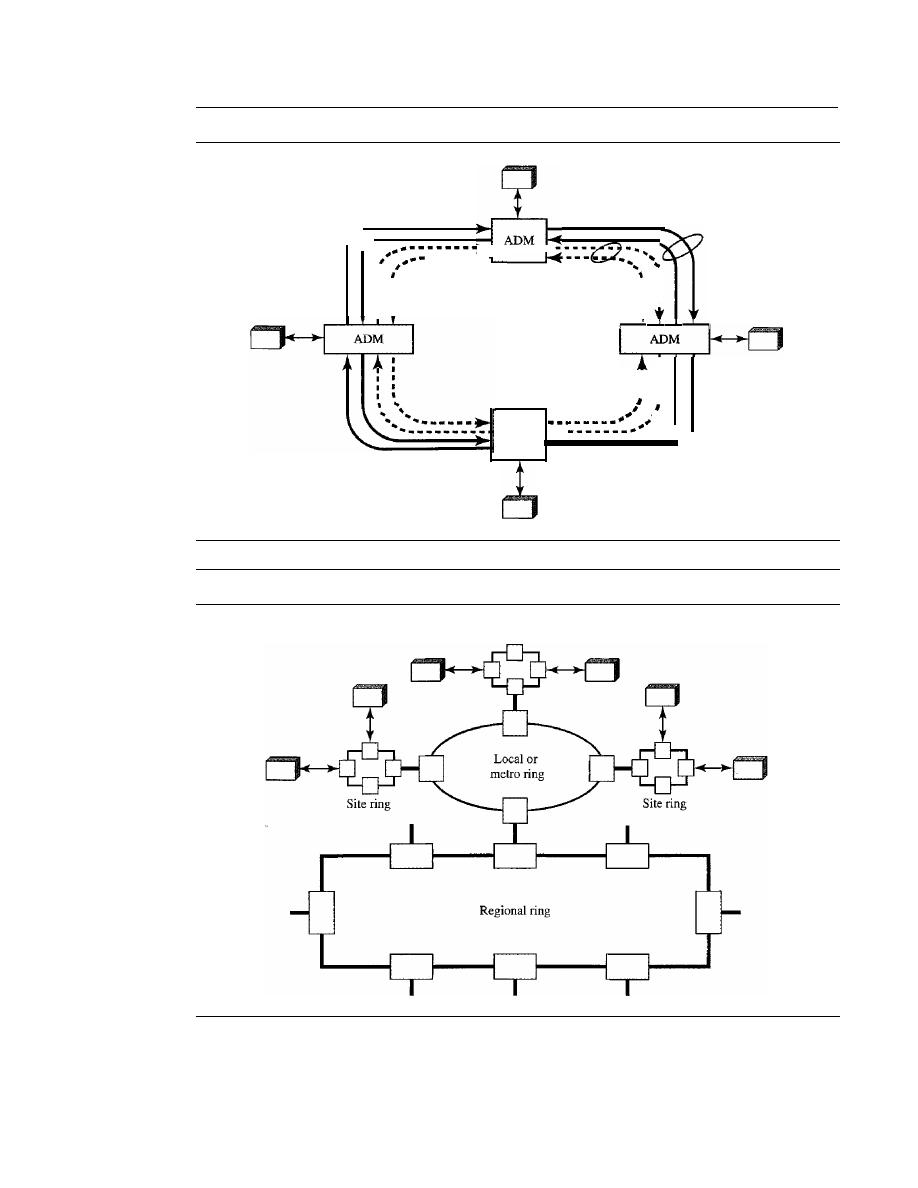
SECTION 17.5
SONET NETWORKS
511
Figure 17.22
A
bidirectional line switching ring
Working
rings
I
•
I
•
I
• •
•
ADM
- - - - - - -
:
Protection
•
:
:
rings
: :
•
I
•
I
I
•
•
Figure 17.23
A combination of rings in a SONET network
Site ring
STS-1 signal to the appropriate output port. An output port takes STS-1 signals coming
from different input ports, multiplexes them into an
STS-n
signal, and makes an
OC-n
signal for transmission. Figure 17.24 shows a mesh SONET network, and the structure of a
switch.
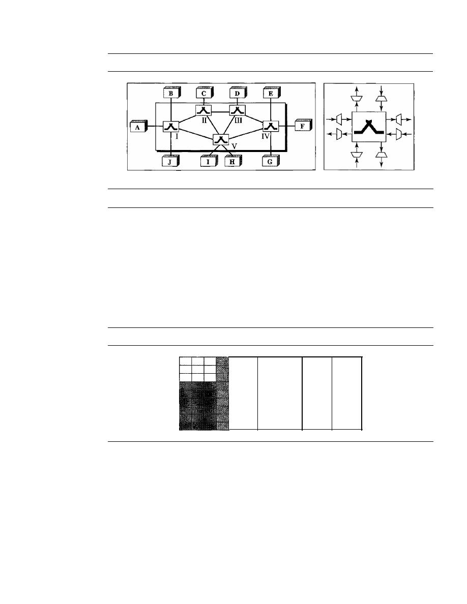
512
CHAPTER 17
SONET/SDH
Figure 17.24
A mesh SONET network
a. SONET mesh network
b. Cross-connect switch
17.6
VIRTUAL TRIBUTARIES
SONET is designed to carry broadband payloads. Current digital hierarchy data rates
(DS-I to DS-3), however, are lower than STS-l. To make SONET backward-compatible
with the current hierarchy, its frame design includes a system of virtual tributaries
(VTs) (see Figure 17.25). A virtual tributary is a partial payload that can be inserted
into an STS-l and combined with other partial payloads to fill out the frame. Instead of
using all 86 payload columns of an STS-l frame for data from one source, we can sub-
divide the SPE and call each component a VT.
Figure 17.25
Virtual tributaries
VT
VT
VT
VT
Types ofVTs
Four types of VTs have been defined to accommodate existing digital hierarchies (see
Figure 17.26). Notice that the number of columns allowed for each type of VT can be
determined by doubling the type identification number (VT1.5 gets three columns, VT2
gets four columns, etc.).
o
VT1.5 accommodates the U.S. DS-I service (1.544 Mbps).
o
VT2 accommodates the European CEPT-l service (2.048 Mbps).
o
VT3 accommodates the DS-IC service (fractional DS-l, 3.152 Mbps).
o
VT6 accommodates the DS-2 service (6.312 Mbps).
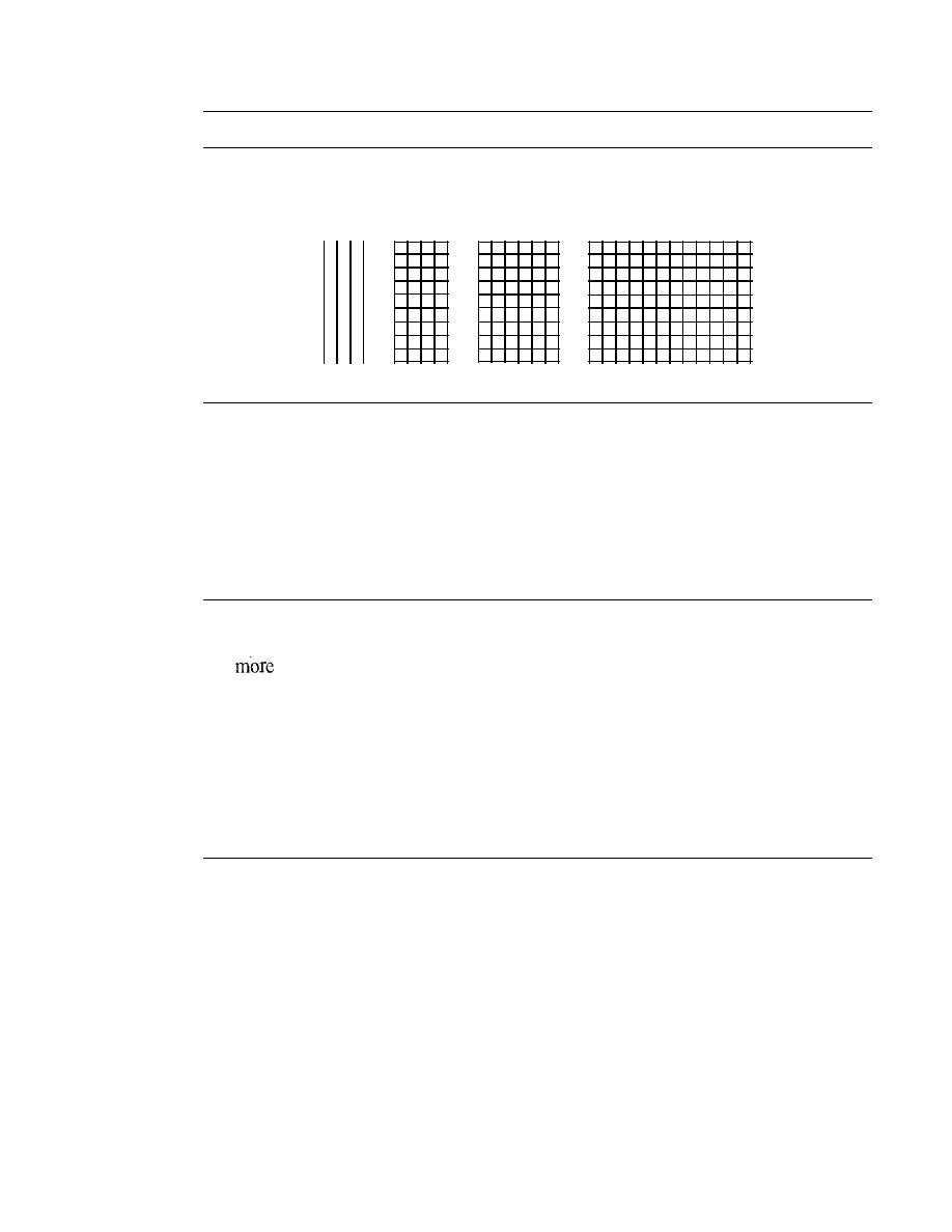
SECTION
17.8
KEY TERMS
513
Figure 17.26
Virtual tributary types
VT1.5
=
8000 frames/s
3 columns
9 rows 8 bits
=
1.728 Mbps
VT2
=
8000 frames/s
4 columns
9 rows 8 bits
=
2.304 Mbps
VT3
=
8000 frarnes/s 6 columns
9 rows 8 bits
=
3.456 Mbps
VT6
=
8000 frames/s 12 columns 9 rows 8 bits
=
6.912 Mbps
VT1.5
VT2
VT3
VT6
When two or more tributaries are inserted into a single STS-1 frame. they are
interleaved column by column. SONET provides mechanisms for identifying each
VT and separating them without demultiplexing the entire stream. Discussion of
these mechanisms and the control issues behind them is beyond the scope of this
book.
17.7
RECOMMENDED READING
For
details about subjects discussed in this chapter, we recommend the following
books. The items in brackets [...] refer to the reference list at the end of the text.
Books
SONET is discussed in Section 2.5 of [Tan03], Section 15.2 of [Kes97], Sections 4.2
and 4.3 of [GW04], Section 8.2 of [Sta04], and Section 5.2 of [WVOOl
17.8
KEY TERMS
add/drop multiplexer (ADM)
automatic protection switching (APS)
bidirectional line switching ring (BLSR)
byte interleaving
line
line layer
line overhead (LOH)
optical carrier (Oe)
path
path layer
path overhead (POH)
photonic layer
regenerator
section
section layer
section overhead (SOH)
STS demultiplexer
STS multiplexer
Synchronous Digital Hierarchy (SDH)
Synchronous Optical Network (SONET)

514
CHAPTER
17
SONETISDH
synchronous payload envelope (SPE)
synchronous transport module (STM)
synchronous transport signal (STS)
terminal
unidirectional path switching ring (UPSR)
virtual tributary (VT)
17.9
SUMMARY
o
Synchronous Optical Network (SONET) is a standard developed by ANSI for
fiber-optic networks: Synchronous Digital Hierarchy (SDH) is a similar standard
developed by ITU-T.
o
SONET has defined a hierarchy of signals called synchronous transport signals
(STSs). SDH has defined a similar hierarchy of signals called synchronous transfer
modules (STMs).
o
An OC-n signal is the optical modulation of an STS-n (or STM-n) signal.
o
SONET defines four layers: path, line, section, and photonic.
o
SONET is a synchronous TDM system in which all clocks are locked to a master
clock.
o
A SONET system can use the following equipment:
1. STS multiplexers
2. STS demultiplexers
3. Regenerators
4. Add/drop multiplexers
5. Terminals
o
SONET sends 8000 frames per second; each frame lasts
125
o
An STS-I frame is made of 9 rows and 90 columns; an STS-n frame is made of
9 rows and n x 90 columns.
o
STSs can be multiplexed to get a new STS with a higher data rate.
D
SONET network topologies can be linear, ring, or mesh.
o
A linear SONET network can be either point-to-point or multipoint.
D
A ring SONET network can be unidirectional or bidirectional.
o
To make SONET backward-compatible with the current hierarchy, its frame design
includes a system of virtual tributaries (VTs).
17.10
PRACTICE SET
Review Questions
I. What is the relationship between SONET and SDH?
2. What is the relationship between STS and STM?
3. How is an STS multiplexer different from an add/drop multiplexer since both can
add signals together?

SECTION 17.10
PRACTICE SET
SIS
4. What is the relationship between STS signals and OC signals?
5. What is the purpose of the pointer in the line overhead?
6. Why is SONET called a synchronous network?
7. What is the function of a SONET regenerator?
8. What are the four SONET layers?
9. Discuss the functions of each SONET layer.
10. What is a virtual tributary?
Exercises
II.
What are the user data rates of STS-3, STS-9, and STS-12?
12. Show how STS-9's can be multiplexed to create an STS-36. Is there any extra
overhead involved in this type of multiplexing?
13. A stream of data is being carried by STS-l frames.
If
the data rate of the stream is
49.540 Mbps, how many STS-l frames per second must let their H3 bytes carry data?
14. A stream of data is being carried by STS-l frames.
If
the data rate of the stream is
49.530 Mbps, how many frames per second should leave one empty byte after the
H3 byte?
IS.
Table 17.2 shows that the overhead bytes can be categorized as A, B, C, D, E, F, G,
H,
J,
K, and Z bytes.
a. Why are there no A bytes in the LOH or POH?
b. Why are there no C bytes in the LOH?
c. Why are there no D bytes in the POH?
d. Why are there no E bytes in the LOH or POR?
e. Why are there no F bytes in the LOH or POH?
f.
Why are there no G bytes in the SOH or LOH?
g. Why are there no H bytes in the SOH?
h. Why are there no
J
bytes in the SOH or LOH?
i. Why are there no K bytes in the SOH or POH?
j.
Why are there no Z bytes in the SOH?
16. Why are B bytes present in all three headers?


CHAPTER 18
Virtual-Circuit Networks:
Frame Relay andATM
In Chapter 8, we discussed switching techniques. We said that there are three types of
switching: circuit switching, packet switching, and message switching. We also men-
tioned that packet switching can use two approaches: the virtual-circuit approach and
the datagram approach.
In this chapter, we show how the virtual-circuit approach can be used in wide-area
networks. Two common WAN technologies use virtual-circuit switching. Frame Relay
is a relatively high-speed protocol that can provide some services not available in other
WAN technologies such as DSL, cable TV, and T lines. ATM, as a high-speed protocol,
can be the superhighway of communication when it deploys physical layer carriers
such as SONET.
We first discuss Frame Relay. We then discuss ATM in greater detaiL Finally, we
show how ATM technology, which was originally designed as a WAN technology, can
also be used in LAN technology, ATM LANs.
18.1
FRAME RELAY
Frame Relay is a virtual-circuit wide-area network that was designed in response to
demands for a new type of WAN in the late 1980s and early 1990s.
1. Prior to Frame Relay, some organizations were using a virtual-circuit switching
network called X.25 that performed switching at the network layer. For example,
the Internet, which needs wide-area networks to carry its packets from one place to
another, used X.25. And X.25 is still being used by the Internet, but it is being
replaced by other WANs. However, X.25 has several drawbacks:
a. X.25 has a low 64-kbps data rate. By the 1990s, there was a need for higher-
data-rate WANs.
b. X.25 has extensive flow and error control at both the data link layer and the
network layer. This was so because X.25 was designed in the 1970s, when
the available transmission media were more prone to errors. Flow and error
control at both layers create a large overhead and slow down transmissions. X.25
requires acknowledgments for both data link layer frames and network layer
packets that are sent between nodes and between source and destination.
517

518
CHAPTER
18
ViRTUAL-CIRCUiT NETWORKS: FRAME RELAY AND ATM
c. Originally X.25 was designed for private lise, not for the Internet. X.25 has its
own network layer. This means that the user's data are encapsulated in the
network layer packets of X.25. The Internet, however, has its own network
layer, which means if the Internet wants to use X.25, the Internet must deliver
its network layer packet, called a datagram, to X.25 for encapsulation in the
X.25 packet. This doubles the overhead.
2. Disappointed with X.25, some organizations started their own private WAN by
leasing T-l or T-3 lines from public service providers. This approach also has some
drawbacks.
a. If an organization has
n
branches spread over an area, it needs
n(n
1)/2 T-I or
T-3 lines. The organization pays for all these lines although it may use the lines
only 10 percent of the time. This can be very costly:
b. The services provided by T-I and T-3 lines assume that the user has fixed-rate
data all the time. For example, a T-l line is designed for a user who wants to
use the line at a consistent 1.544 Mbps. This type of service is not suitable for
the many users today that need to send
bursty data. For example, a user may
want to send data at 6 Mbps for 2 s, 0 Mbps (nothing) for 7 s, and 3.44 Mbps
for 1 s for a total of 15.44 Mbits during a period of 10 s. Although the average
data rate is still 1.544 Mbps, the T-I line cannot accept this type of demand
because it is designed for fixed-rate data, not bursty data. Bursty data require
what is called
bandwidth on demand. The user needs different bandwidth
allocations at different times.
In response to the above drawbacks, Frame Relay was designed. Frame Relay is a wide-
area network with the following features:
1. Frame Relay operates at a higher speed (1.544 Mbps and recently 44.376 Mbps).
This means that it can easily be used instead of a mesh of T-I or T-3 lines.
2. Frame Relay operates in just the physical and data link layers. This means it can
easily be used as a backbone network to provide services to protocols that already
have a network layer protocol, such as the Internet.
3. Frame Relay allows bursty data.
4. Frame Relay allows a frame size of 9000 bytes, which can accommodate all local-
area network frame sizes.
5. Frame Relay is less expensive than other traditional WANs.
6. Frame Relay has error detection at the data link layer only. There is no flow control
or error control. There is not even a retransmission policy if a frame is damaged; it
is silently dropped. Frame Relay was designed in this way to provide fast transmis-
sion capability for more reliable media and for those protocols that have flow and
error control at the higher layers.
Architecture
Frame Relay provides permanent virtual circuits and switched virtual circuits. Figure 18.1
shows an example of a Frame Relay network connected to the Internet. The routers are
used, as we will see in Chapter 22, to connect LANs and WANs in the Internet. In the
figure, the Frame Relay WAN is used as one link in the global Internet.
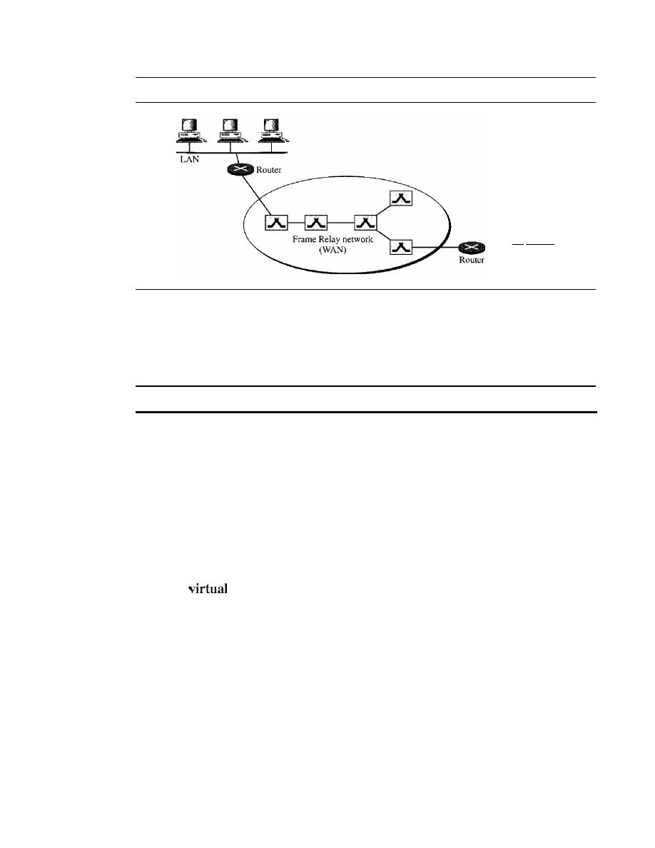
SECTION
18.1
FRAME RELAY
519
Figure 18.1
Frame Relay network
To the rest of
the Internet
Virtual Circuits
Frame Relay is a virtual circuit network. A virtual circuit in Frame Relay is identified
by a number called a
data link connection identifier (DLCI).
VCIs in Frame Relay are called DLCIs.
Permanent Versus Switched Virtual Circuits
A source and a destination may choose to have a
permanent virtual circuit (PVC). In
this case, the connection setup is simple. The corresponding table entry is recorded for
all switches by the administrator (remotely and electronically, of course). An outgoing
DLCI is given to the source, and an incoming DLCI is given to the destination.
PVC connections have two drawbacks. First, they are costly because two parties
pay for the connection all the time even when it is not in use. Second, a connection is
created from one source to one single destination.
If
a source needs connections with
several destinations, it needs a PVC for each connection. An alternate approach is the
switched
circuit (SVC). The SVC creates a temporary, short connection that
exists only when data are being transferred between source and destination. An SVC
requires establishing and terminating phases as discussed in Chapter 8.
Switches
Each switch in a Frame Relay network has a table to route frames. The table matches
an incoming port-DLCI combination with an outgoing port-DLCI combination as we
described for general virtual-circuit networks in Chapter 8. The only difference is that
VCIs are replaced by DLCIs.
Frame Relay Layers
Figure 18.2 shows the Frame Relay layers. Frame Relay has only physical and data link
layers.
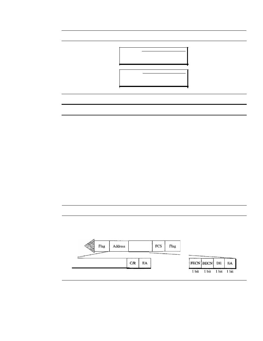
520
CHAPTER
18
VIRTUAL-CIRCUIT NETWORKS: FRAME RELAY AND ATM
Figure 18.2
Frame Relay layers
Data link
Ph sical
I
Simplified core functions
I
of data link layer
ANSI standards
Frame Relay operates only at the physical and data link layers.
Physical Layer
No specific protocol is defined for the physical layer in Frame Relay. Instead, it is left
to the implementer to use whatever is available. Frame Relay supports any of the proto-
cols recognized by ANSI.
Data Link Layer
At the data link layer, Frame Relay uses a simple protocol that does not support flow or
error control. It only has an error detection mechanism. Figure 18.3 shows the format
of a Frame Relay frame.The address field defines the DLCI as well as some bits used to
control congestion.
Figure 18.3
Frame Relay frame
C/R:
Command/response
EA: Extended address
FECN: Forward explicit congestion notification
BECN: Backward explicit congestion notification
DE: Discard eligibility
DLCI: Data link connection identifier
DLCI
6 bits
Information
1 bit
1 bit
DLCI
4 bits
The descriptions of the fields are as follows:
o
Address (DLCI) field. The first 6 bits of the first byte makes up the first part of the
DLCI. The second part of the DLCI uses the first 4 bits of the second byte. These
bits are part of the lO-bit data link connection identifier defined by the standard.
We will discuss extended addressing at the end of this section.

SECTION
18.1
FRAME RELAY
521
o
Command/response (CIR).
The command/response (C/R) bit is provided to allow
upper layers to identify a frame as either a command or a response.
It
is not used
by the Frame Relay protocol.
o
Extended address (EA).
The extended address (EA) bit indicates whether the
current byte is the final byte of the address. An EA of 0 means that another address
byte is
to
follow (extended addressing is discussed later). An EA of 1 means that
the current byte is the final one.
o
Forward explicit congestion notification (FECN).
The
forward explicit con-
gestion notification (FECN)
bit can be set by any switch to indicate that traffic
is congested. This bit informs the destination that congestion has occurred. In this
way, the destination knows that it should expect delay or a loss of packets. We will
discuss the use of this bit when we discuss congestion control in Chapter 24.
o
Backward explicit congestion notification (BECN).
The
backward explicit con-
gestion notification (BECN)
bit is set (in frames that travel in the other direction) to
indicate a congestion problem in the network. This bit informs the sender that con-
gestion has occurred. In this way, the source knows it needs to slow down to prevent
the loss of packets. We will discuss the use of
bit when we discuss congestion
control in Chapter 24.
o
Discard eligibility (DE).
The
discard eligibility (DE)
bit indicates the priority
level of the frame. In emergency situations, switches may have to discard frames to
relieve bottlenecks and keep the network from collapsing due to overload. When set
(DE
1),
this bit tells the network to discard
frame if there is congestion. This bit
can be set either by the sender of the frames (user) or by any switch in the network.
Frame Relay does not provide flow or error control;
they must be provided by the upper-layer protocols.
Extended Address
To increase the range of DLCIs, the Frame Relay address has been extended from the
original 2-byte address to
or 4-byte addresses. Figure 18.4 shows the different
addresses. Note that the EA field defines the number of bytes; it is 1 in the last byte of
the address, and it is
a
in the other bytes. Note that in the 3- and 4-byte formats, the bit
before the last bit is set to O.
Figure 18.4
Three address formats
DLCI
a. Two-byte address (lO-bit DLCI)
DLCI
CIR
EA=O
OLCI
IFECNIBECN
DE
EA=O
DLCI
0
EA= I
b. Three-byte address (16-bit DLCI)
OLCI
ICIR
EA=O
OLCI
I
PECN IBECN I OE
EA=O
DLCI
EA=O
DLCI
I
0
EA= 1
c. Four-byte address (23-bit DLCI)
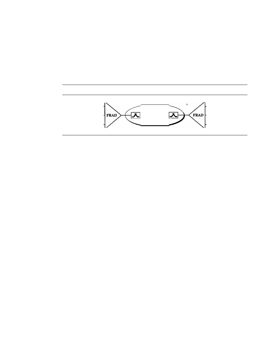
522
CHAPTER
18
VIRTUAL-CIRCUIT NETWORKS: FRAME RELAY AND ATM
FRADs
To handle frames arriving from other protocols, Frame Relay uses a device called a
Frame Relay assembler/disassembler (FRAD). A FRAD assembles and disassembles
frames coming from other protocols to allow them to be carried by Frame Relay frames.
A FRAD can be implemented as a separate device or as part of a switch. Figure 18.5
shows two FRADs connected to a Frame Relay network.
Figure 18.5
FRAD
X.25
ATM
ppp
VOFR
Frame
Relay
X.25
ATM
ppp
Frame Relay networks offer an option called
Voice Over Frame Relay (VOFR) that
sends voice through the network. Voice is digitized using PCM and then compressed.
The result is sent as data frames over the network. This feature allows the inexpensive
sending of voice over long distances. However, note that the quality of voice is not as
good as voice over a circuit-switched network such as the telephone network. Also, the
varying delay mentioned earlier sometimes corrupts real-time voice.
LMI
Frame Relay was originally designed to provide PVC connections. There was not,
therefore, a provision for controlling or managing interfaces.
Local Management
Information (LMI) is a protocol added recently to the Frame Relay protocol to pro-
vide more management features. In particular, LMI can provide
o
A keep-alive mechanism to check if data are flowing.
o
A multicast mechanism to allow a local end system to send frames to more than
one remote end system.
o
A mechanism to allow an end system to check the status of a switch (e.g., to see if
the switch is congested).
Congestion Control and Quality of Service
One of the nice features of Frame Relay is that it provides
congestion control and
quality of service (QoS). We have not discussed these features yet. In Chapter 24, we
introduce these two important aspects of networking and discuss how they are imple-
mented in Frame Relay and some other networks.

SECTION
18.2
ATM
523
18.2
ATM
Asynchronous Transfer Mode (ATM) is the cell relay protocol designed by the ATM
Forum and adopted by the ITU-T. The combination of ATM and SONET will allow
high-speed interconnection of all the world's networks. In fact, ATM can be thought of
as the "highway" of the information superhighway.
Design Goals
Among the challenges faced by the designers of ATM, six stand out.
1. Foremost is the need for a transmission system to optimize the use of high-data-rate
transmission media, in particular optical fiber. In addition to offering large band-
widths, newer transmission media and equipment are dramatically less susceptible
to noise degradation. A technology is needed to take advantage of both factors and
thereby maximize data rates.
2. The system must interface with existing systems and provide wide-area intercon-
nectivity between them without lowering their effectiveness or requiring their
replacement.
3. The design must be implemented inexpensively so that cost would not be a barrier
to adoption. If ATM is to become the backbone of international communications,
as intended, it must be available at low cost to every user who wants it.
4. The new system must be able to work with and support the existing telecom-
munications hierarchies (local loops, local providers, long-distance carriers, and
so on).
5. The new system must be connection-oriented to ensure accurate and predictable
delivery.
6. Last but not least, one objective is to move as many of the functions to hardware as
possible (for speed) and eliminate as many software functions as possible (again
for speed).
Before we discuss the solutions to these design requirements, it is useful to examine some
of the problems associated with existing systems.
Frame Networks
Before ATM, data communications at the data link layer had been based on frame
switching and frame networks. Different protocols use frames of varying size and intri-
cacy. As networks become more complex, the information that must be carried in the
header becomes more extensive. The result is larger and larger headers relative to the
size of the data unit. In response, some protocols have enlarged the size of the data unit
to make header use more efficient (sending more data with the same size header).
Unfortunately, large data fields create waste. If there is not much information to transmit,
much of the field goes unused. To improve utilization, some protocols provide variable
frame sizes to users.
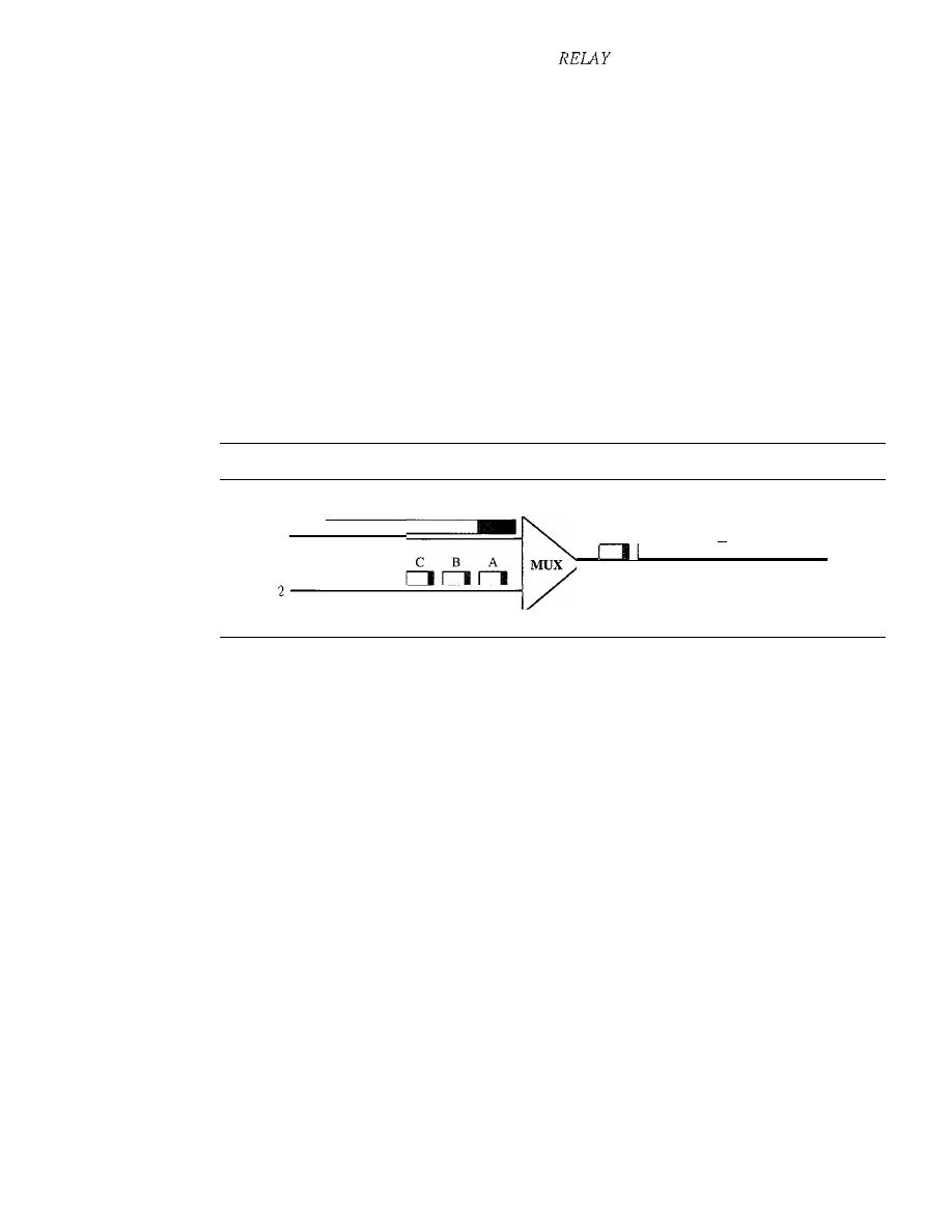
524
CHAPTER
18
VIRTUAL-CIRCUIT NETWORKS: FRAME
AND ATM
Mixed Network Traffic
As you can imagine, the variety of frame sizes makes traffic unpredictable. Switches,
multiplexers, and routers must incorporate elaborate software systems to manage the
various sizes of frames. A great deal of header information must be read, and each bit
counted and evaluated to ensure the integrity of every frame. Internetworking among
the different frame networks is slow and expensive at best, and impossible at worst.
Another problem is that of providing consistent data rate delivery when frame
sizes are unpredictable and can vary so dramatically. To get the most out of broadband
technology, traffic must be time-division multiplexed onto shared paths. Imagine the
results of multiplexing frames from two networks with different requirements (and
frame designs) onto one link (see Figure 18.6). What happens when line 1 uses large
frames (usually data frames) while line 2 uses very small frames (the norm for audio
and video information)?
Figure 18.6
Multiplexing using different frame sizes
x
A
x
If line 1's gigantic frame X arrives at the multiplexer even a moment earlier than
line 2's frames, the multiplexer puts frame X onto the new path first. After all, even if
line 2's frames have priority, the multiplexer has no way of knowing to wait for them
and so processes the frame that has arrived. Frame A must therefore wait for the entire
X bit stream to move into place before it can follow. The sheer size of X creates an
unfair delay for frame A. The same imbalance can affect all the frames from line 2.
Because audio and video frames ordinarily are small, mixing them with conven-
tional data traffic often creates unacceptable delays of this type and makes shared frame
links unusable for audio and video information. Traffic must travel over different paths,
in much the same way that automobile and train traffic does. But to fully utilize broad
bandwidth links, we need to be able to send all kinds of traffic over the same links.
Cell Networks
Many of the problems associated with frame internetworking are solved by adopting
a concept called cell networking. A cell is a small data unit of fixed size. In a
cell
network, which uses the
cell
as the basic unit of data exchange, all data are loaded into
identical cells that can be transmitted with complete predictability and uniformity. As
frames of different sizes and formats reach the cell network from a tributary network,
they are split into multiple small data units of equal length and are loaded into cells.
The cells are then multiplexed with other cells and routed through the cell network.
Because each cell is the same size and all are small, the problems associated with
multiplexing different-sized frames are avoided.
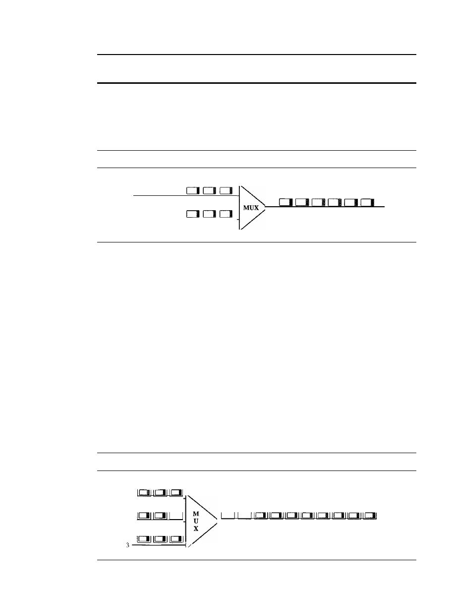
SECTION
18.2
ATM
525
A cell network uses the cell as the basic unit of data exchange.
A cell is defined as a small, fixed-size block of information.
Figure 18.7 shows the multiplexer from Figure 18.6 with the two lines sending
cells instead of frames. Frame X has been segmented into three cells: X, Y, and Z. Only
the first cell from line 1 gets put on the link before the first cell from line 2. The cells
from the two lines are interleaved so that none suffers a long delay.
Figure 18.7
Multiplexing using cells
z
y
x
C
B
A
2------=-----;
C
Z
B
Y
A
x
A second point in this same scenario is that the high speed of the links coupled
with the small size of the cells means that, despite interleaving, cells from each line
arrive at their respective destinations in an approximation of a continuous stream (much
as a movie appears to your brain to be continuous action when in fact it is really a series
of separate, still photographs). In this way, a cell network can handle real-time trans-
missions, such as a phone call, without the parties being aware of the segmentation or
multiplexing at all.
Asynchronous TDM
ATM uses asynchronous time-division multiplexing-that is why it is called Asynchro-
nous Transfer Mode-to multiplex cells corning from different channels.
It
uses fixed-size
slots (size of a cell). ATM multiplexers fill a slot with a cell from any input channel that
has a cell; the slot is empty if none of the channels has a cell to send.
Figure 18.8 shows how cells from three inputs are multiplexed. At the first tick of
the clock: channel 2 has no cell (empty input slot), so the multiplexer fills the slot with
a cell from the third channel. When all the cells from all the channels are multiplexed,
the output slots are empty.
Figure 18.8
ATM multiplexing
A3
A2
Al
B2
81
2 - - - - - - - - 1
C3
C2
Cl
C3
82
A3
C2
Bl
A2
Cl
Ai
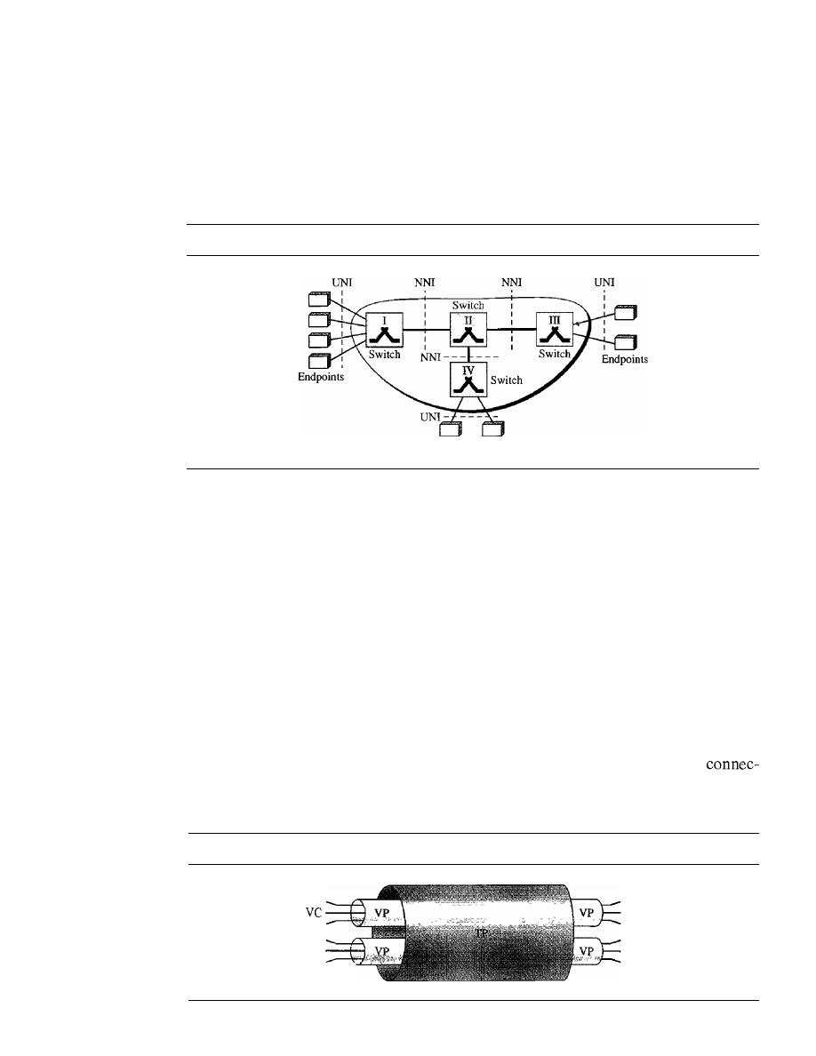
526
CHAPTER
18
VIRTUAL-CIRCUIT NETWORKS: FRAME RELAY AND ATM
Architecture
ATM is a cell-switched network. The user access devices, called the endpoints, are
connected through a
user-to-network interface (UNI) to the switches inside the net-
work. The switches are connected through
network-to-network interfaces (NNIs).
Figure 18.9 shows an example of an ATM network.
Figure 18.9
Architecture of an ATM network
Endpoints
Virtual Connection
Connection between two endpoints is accomplished through transmission paths (TPs),
virtual paths (YPs), and virtual circuits (YCs). A
transmission path (TP) is the physical
connection (wire, cable, satellite, and so on) between an endpoint and a switch or
between two switches. Think of two switches as two cities. A transmission path is the
set of all highways that directly connect the two cities.
A transmission path is divided into several virtual paths. A
virtual path (VP) pro-
vides a connection or a set of connections between two switches. Think of a virtual path
as a highway that connects two cities. Each highway is a virtual path; the set of all
highways is the transmission path.
Cell networks are based on
virtual circuits (VCs). All cells belonging to a single
message follow the same virtual circuit and remain in their original order until they
reach their destination. Think of a virtual circuit as the lanes of a highway (virtual path).
Figure 18.10 shows the relationship between a transmission path (a physical
tion), virtual paths (a combination of virtual circuits that are bundled together because
parts of their paths are the same), and virtual circuits that logically connect two points.
Figure 18.10
Tp, VPs, and VCs
VC
VC
VC
VC
VC
vc
vc
VC
VC
VC
VC
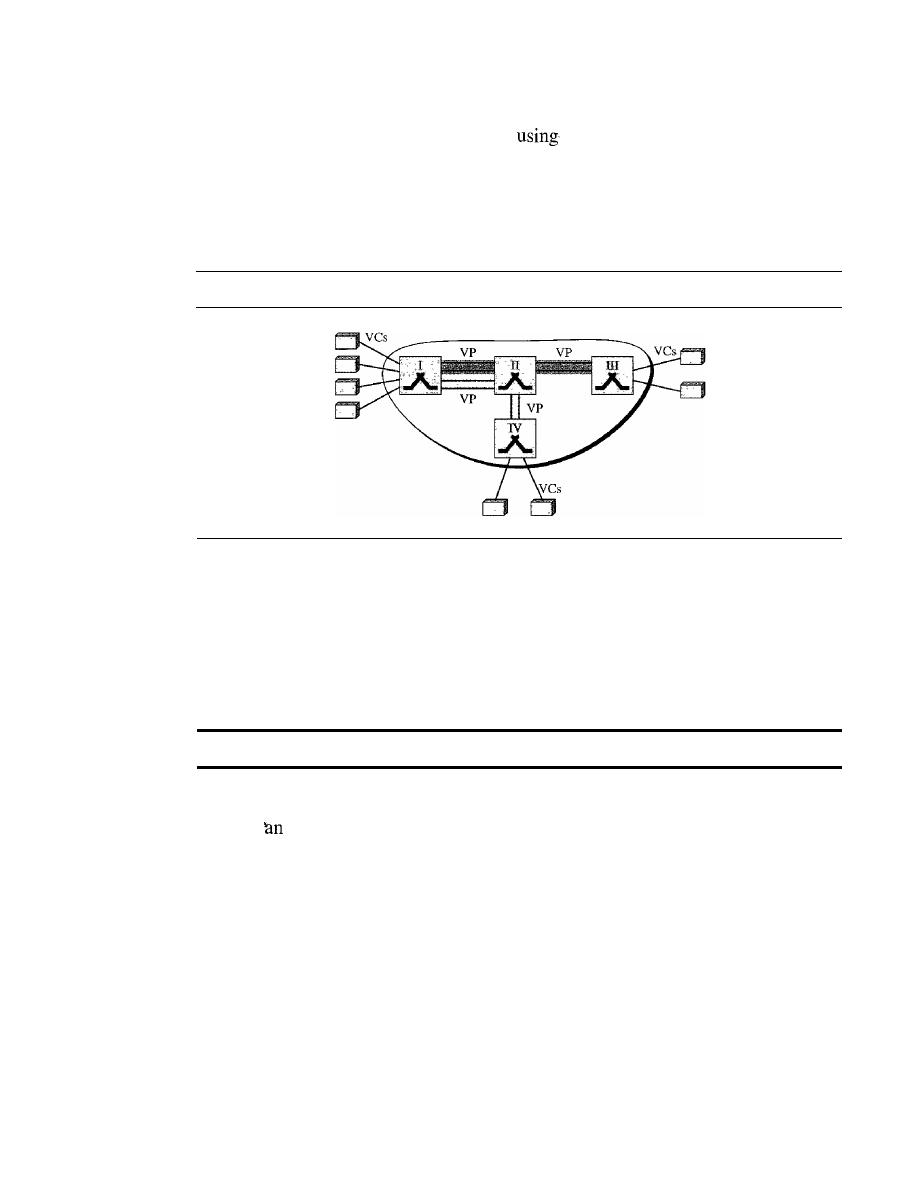
SECTION
18.2
ATM
527
To better understand the concept of VPs and VCs, look at Figure 18.11. In this
figure, eight endpoints are communicating
four VCs. However, the first two VCs
seem to share the same virtual path from switch I to switch III, so it is reasonable to
bundle these two VCs together to form one VP. On the other hand, it is clear that the
other two VCs share the same path from switch I to switch IV, so it is also reasonable to
combine them to form one VP.
Figure 18.11
Example ofVPs and VCs
Identifiers
In a virtual circuit network, to route data from one endpoint to another,
the virtual connections need to be identified. For this purpose, the designers of ATM
created a hierarchical identifier with two levels: a
virtual path identifier (VPI) and a
virtual-circuit identifier (Vel). The VPI defines the specific VP, and the Vel defines a
particular VC inside the VP. The VPI is the same for all virtual connections that are
bundled (logically) into one VP.
Note that a virtual connection is defined
by a pair of numbers: the VPI and the vel.
Figure 18.12 shows the VPIs and VCls for a transmission path. The rationale for
dividing
identifier into two parts will become clear when we discuss routing in an
ATM network.
The lengths of the VPIs for UNIs and NNIs are different. In a UNI, the VPI is
8 bits, whereas in an NNI, the VPI is 12 bits. The length of the VCI is the same in both
interfaces (16 bits). We therefore can say that a virtual connection is identified by
24 bits in a UNI and by 28 bits in an NNI (see Figure 18.13).
The whole idea behind dividing a virtual circuit identifier into two parts is to allow
hierarchical routing. Most of the switches in a typical ATM network are routed using
VPIs. The switches at the boundaries of the network, those that interact directly with
the endpoint devices, use both VPIs and VCIs.
Cells
The basic data unit in an ATM network is called a cell. A cell is only 53 bytes long with
5 bytes allocated to the header and 48 bytes carrying the payload (user data may be less
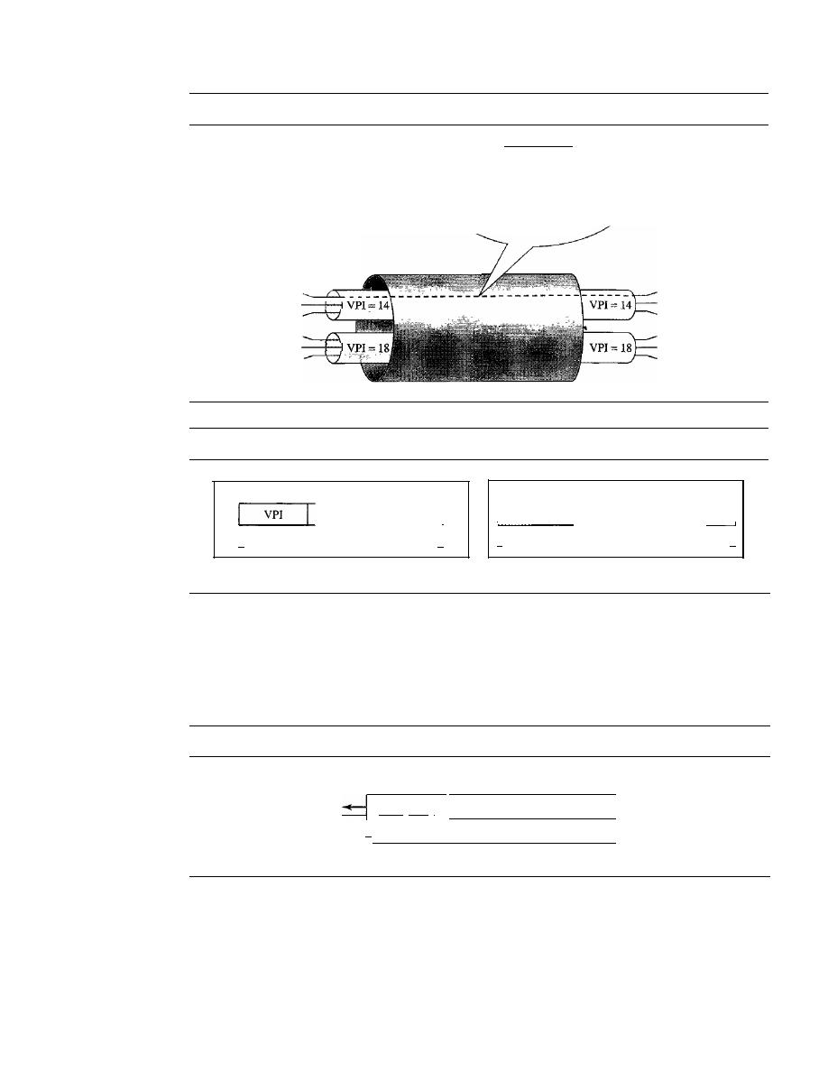
528
CHAPTER
18
VIRTUAL-CIRCUIT NETWORKS: FRAME RELAY AND ATM
Figure 18.12
Connection identifiers
This virtual connection is
uniquely defined using the pair:
(14
21)
t t
VPl VCl
VCl=21
VCl = 32
VCl=45
VCl=70
VCl=74
VCl=45
Figure 18.13
Virtual connection identifiers in UNIs and NNIs
VCl=21
VCl= 32
VCl=45
VCl=70
VCl=74
VCl=45
V_C_I
1
I-
24 bits
·1
8
bits
16 bits
12 bits
16 bits
I
VPl
VCl
I
I-
28 bits
-,
a. VPI and
VCI in a UNI
b. VPI and VCI in an NNI
than 48 bytes). We will study in detail the fields of a cell, but for the moment it suffices
to say that most of the header is occupied by the VPI and VCI that define the virtual
connection through which a cell should travel from an endpoint to a switch or from a
switch to another switch. Figure 18.14 shows the cell structure.
Figure 18.14
An ATM cell
Header
IVPII VCI I
I,
5 bytes
Connection Establishment and Release
53 bytes
Payload
48 bytes
Like Frame Relay, ATM uses two types of connections: PVC and SVc.
PVC
A permanent virtual-circuit connection is established between two endpoints by
the network provider. The VPls and vcrs are defined for the permanent connections,
and the values are entered for the tables of each switch.
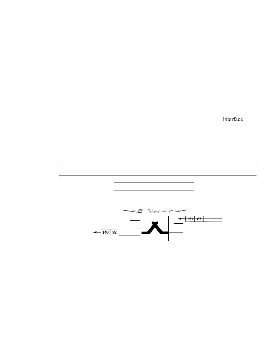
SECTION
18.2
ATM
529
SVC
In a switched virtual-circuit connection, each time an endpoint wants to make a
connection with another endpoint, a new virtual circuit must be established. ATM cannot
do the job by itself, but needs the network layer addresses and the services of another pro-
tocol (such as IP). The signaling mechanism of this other protocol makes a connection
request by using the network layer addresses of the two endpoints. The actual mechanism
depends on the network layer protocol.
Switching
ATM uses switches to route the cell from a source endpoint to the destination endpoint.
A switch routes the cell using both the VPls and the VCls. The routing requires the
whole identifier. Figure 18.15 shows how a VPC switch routes the cell. A cell with a
VPI of 153 and VCI of 67 arrives at switch interface (port) 1. The switch checks its
switching table, which stores six pieces of information per row: arrival
num-
ber, incoming VPI, incoming VCI, corresponding outgoing interface number, the new
VPI, and the new VCL The switch finds the entry with the interface 1, VPI 153, and
VCI 67 and discovers that the combination corresponds to output interface 3, VPI 140,
and VCI 92.
It
changes the VPI and VCI in the header to 140 and 92, respectively, and
sends the cell out through interface 3.
Figure 18.15
Routing with a switch
VCI
Input
Output
Interface
VPI
VCI Interface
VPI
VCI
1
153
67
3
140
92
.....
.....
.....
..
...
...
.....
VPI
153
4
C1
1
92
I
2
3
VPI V
Switching Fabric
The switching technology has created many interesting features to increase the speed of
switches to handle data. We discussed switching fabrics in Chapter 8.
ATM Layers
The ATM standard defines three layers. They are, from top to bottom, the application
adaptation layer, the ATM layer, and the physical layer (see Figure 18.16).
The endpoints use all three layers while the switches use only the two bottom layers
(see Figure 18.17).
Physical Layer
Like Ethernet and wireless LANs, ATM cells can be carried by any physical layer carrier.
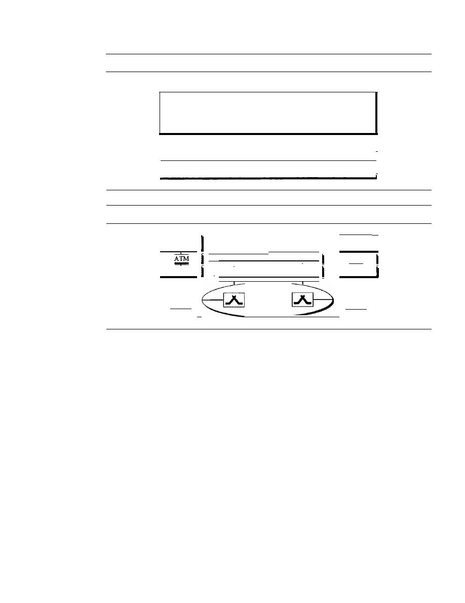
530
CHAPTER
18
VIRTUAL-CIRCUIT NETWORKS: FRAME RELAY AND ATM
Figure
18.16
ATM layers
AAL
AALl
AAL2
AAL3/4
AAL5
ATMlayer
I
- - - - - -
Physical layer
I
Figure
18.17
ATM layers in endpoint devices and switches
AAL
AAL
I
ArM
ATM
ATM
i
,
Physical
I
Physical
Physical
Physical
I
I
I
I
I
I
I
I
D
D
SONET
The original design of ATM was based on SONET (see Chapter 17) as the
physical layer carrier. SONET is preferred for two reasons. First, the high data rate
of SONET's carrier reflects the design and philosophy of ATM. Second, in using
SONET, the boundaries of cells can be clearly defined. As we saw in Chapter 17,
SONET specifies the use of a pointer to define the beginning of a payload. If the begin-
ning of the first ATM cell is defined, the rest of the cells in the same payload can easily
be identified because there are no gaps between cells. Just count 53 bytes ahead to find
the next cell.
Other Physical Technologies
ATM does not limit the physical layer to SONET.
Other technologies, even wireless, may be used. However, the problem of cell bound-
aries must be solved. One solution is for the receiver to guess the end of the cell and
apply the CRC to the 5-byte header. If there is no error, the end of the cell1s found, with a
high probability, correctly. Count 52 bytes back to find the beginning of the cell.
ATM Layer
The ATM layer provides routing, traffic management, switching, and multiplexing
services.
It
processes outgoing traffic by accepting 48-byte segments from the AAL
sublayers and transforming them into 53-byte cells by the addition of a 5-byte header
(see Figure 18.18).
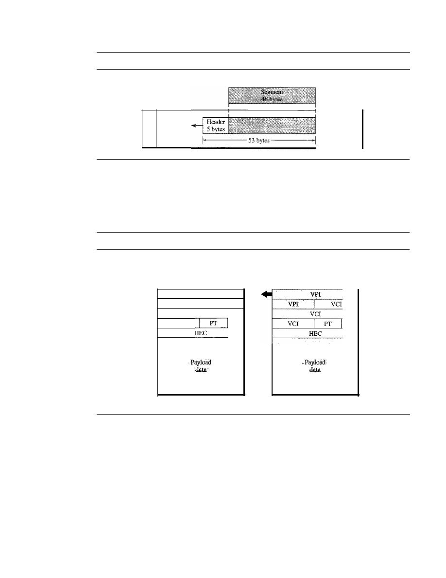
SECTION
18.2
ATM
531
Figure 18.18
ATM
layer
FromAAL
A
T
M
Header Format
ATM uses two fonnats for this header, one for user-to-network inter-
face (UNI) cells and another for network-to-network interface (NNI) cells. Figure 18.19
shows these headers in the byte-by-byte format preferred by the ITU-T (each row repre-
sents a byte).
Figure 18.19
ATM
headers
GFC: Generic flow control
VPl: Virtual path identifier
VCl: Virtual circuit identifier
PT: Payload type
CLP: Cell loss priority
HEC: Header error control
GFC
VPI
VCI
VPI
VCI
VCI
UNI cell
CLP
NNI cell
CLP
o
Generic flow control (GFC).
The 4-bit GFC field provides flow control at the
UNI level. The ITU-T has determined that this level of flow control is not neces-
sary at the NNI level. In the NNI header, therefore, these bits are added to the VPI.
The longer VPI allows more virtual paths to be defined at the NNI level. The
format for this additional VPI has not yet been determined.
o
Virtual path identifier (VPI).
The VPI is an 8-bit field in a UNI cell and a 12-bit
field in an NNI cell (see above).
o
Virtual circuit identifier (VCI).
The VCI is a 16-bit field in both frames.
o
Payload type (PT).
In the 3-bit PT field, the first bit defines the payload as user
data or managerial information. The interpretation of the last 2 bits depends on the
first bit.

532
CHAPTER
18
VIRTUAL-CIRCUIT NETWORKS: FRAME RELAY AND ATM
o
Cell loss priority (CLP). The I-bit CLP field is provided for congestion control. A
cell with its CLP bit set to I must be retained as long as there are cells with a CLP of
O.
We discuss congestion control and quality of service in an ATM network in Chapter 24.
o
Header error correction (HEC). The HEC is a code computed for the first
4 bytes of the header.
It
is a CRC with the divisor
x
8
+
x
2
+
x
+
1 that is used to
correct single-bit errors and a large class of multiple-bit errors.
Application Adaptation Layer
The application adaptation layer (AAL) was designed to enable two ATM concepts.
First, ATM must accept any type of payload, both data frames and streams of bits. A
data frame can come from an upper-layer protocol that creates a clearly defined frame
to be sent to a carrier network such as ATM. A good exampre is the Internet. ATM must
also carry multimedia payload. It can accept continuous bit streams and break them
into chunks to be encapsulated into a cell at the ATM layer. AAL uses two sublayers to
accomplish these tasks.
Whether the data are a data frame or a stream of bits, the payload must be seg-
mented into 48-byte segments to be carried by a cell. At the destination, these segments
need to be reassembled to recreate the original payload. The AAL defines a sublayer,
called a segmentation and reassembly (SAR) sublayer, to do so. Segmentation is at
the source; reassembly, at the destination.
Before data are segmented by SAR, they must be prepared to guarantee the integrity
of the data. This is done by a sublayer called the convergence sublayer (CS).
ATM defines four versions of the AAL:
AALl, AAL2, AAL3/4, and AAL5.
Although we discuss all these versions, we need to inform the reader that the common
versions today are AAL I and AAL5. The first is used in streaming audio and video
communication; the second, in data communications.
AALI
AALI supports applications that transfer information at constant bit rates,
such as video and voice. It allows ATM to connect existing digital telephone networks
such as voice channels and T lines. Figure 18.20 shows how a bit stream of data is
chopped into 47-byte chunks and encapsulated in cells.
The CS sublayer divides the bit stream into 47-byte segments and passes them to
the SAR sublayer below. Note that the CS sublayer does not add a header.
The SAR sublayer adds 1 byte of header and passes the 48-byte segment to the
ATM layer. The header has two fields:
o
Sequence number (SN). This 4-bit field defines a sequence number to order the
bits. The first bit is sometimes used for timing, which leaves 3 bits for sequencing
(modulo 8).
o
Sequence number protection (SNP). The second 4-bit field protects the first
field. The first 3 bits automatically correct the SN field. The last bit is a parity bit
that detects error over all 8 bits.
AAL2
Originally AAL2 was intended to support a variable-data-rate bit stream, but it
has been redesigned.
It
is now used for low-bit-rate traffic and short-frame traffic such
as audio (compressed or uncompressed), video, or fax. A good example of AAL2 use is
in mobile telephony. AAL2 allows the multiplexing of short frames into one cell.
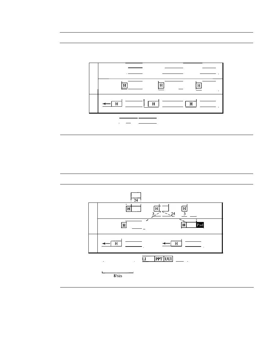
SECTION
18.2
ATM
533
Figure 18.20
AALl
Constant-bit-rate data from upper layer
...................... 1110010010001111
111110101010101
..
A
I
I
CS
I
I
I
I
I
A
47 bytes
47 bytes:
47 bytes:
I
I
L
I
I
SAR
1
I
1
47 bytes
I
1 47 bytes
I
I I
47 bytes
I
I
I
I
I
I
A
I
I
T
I
I
M
5
48 bytes
I
5
48 bytes
1
5
48 bytes
I
SAR header
I
SN
4 bits
SNP
4 bits
SN: Sequence number
SNP: Sequence number protection
UUI: User-to-user indication
HEC: Header error control
SF: Start field
Figure 18.21 shows the process of encapsulating a short frame from the same source
(the same user of a mobile phone) or from several sources (several users of mobile tele-
phones) into one cell.
Figure 18.21
AAL2
Short packets
from upper layer
A
24
1
CS
A
13
24
1
I
L
r
SAR
2
I
1
47 bytes
1
1
1
47 bytes
I
I
1
1
I
A
I
I
T
M
5
48 bytes
5
48 bytes
CS header
I__
C_ID
I__
HEC
I
8 bits
6
2
3
5
SAR header
I
SF
I
CID: Channel identifier
LI:
Length indicator
PPT: Packet payload type
The CS layer overhead consists of five fields:
o
Channel identifier (CID).
The 8-bit CID field defines the channel (user) of the
short packet.
o
Length indicator (LI).
The 6-bit LI field indicates how much of the final packet
is data.
o
Packet payload type (PPT).
The PPT field defines the type of packet.
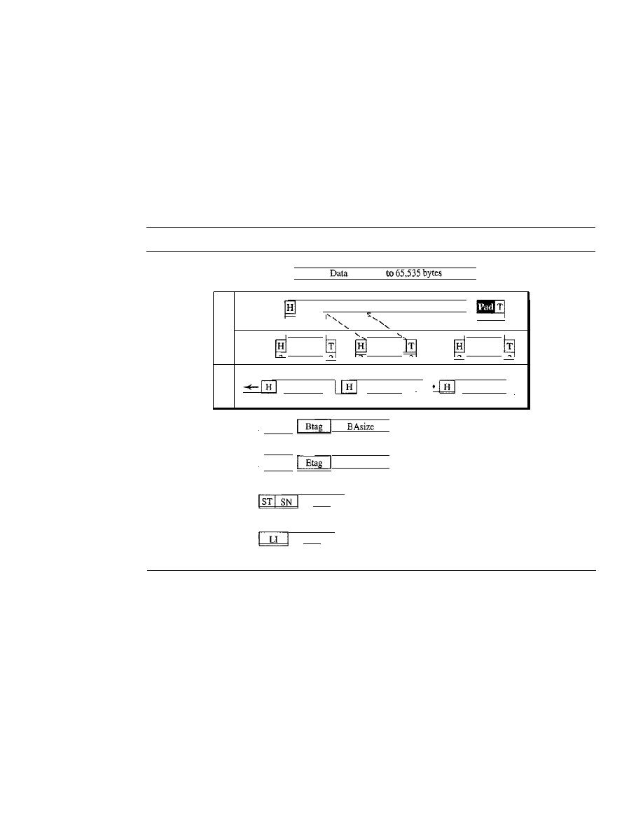
534
CHAPTER
18
VIRTUAL-CIRCUIT NETWORKS: FRAME RELAY AND ATM
o
User-to-user indicator (UUI). The UUI field can be used by end-to-end users.
o
Header error control (HEC). The last 5 bits is used to correct errors in the header.
The only overhead at the SAR layer is the start field (SF) that defines the offset from
the beginning of the packet.
AAL3/4
Initially, AAL3 was intended to support connection-oriented data services and
AAL4 to support connectionless services. As they evolved, however,
it
became evident
that the fundamental issues of the two protocols were the same. They have therefore been
combined into a single format calledAAL3/4. Figure 18.22 shows the AAL3/4 sublayer.
Figure 18.22
AAL3/4
packet
up
I
A
I
1
cs
Data
I
A
I
1
I
I
L
SAR
o
0
0
3/4
1
2
44
2
1
12
44
2
1
1
2
44
2
1
:
I
:
I
I
1
A
I
I
1
1
T
I..
I
M
5
48 bytes
5
48 bytes
5
48 bytes
CS header
I
CPI
8 bits
8
CS trailer
I
AL
8 bits
8
16
L
16
CPI: Common part identifier
Btag: Beginning tag
BAsize: Buffer allocation size
AL:
Alignment
Etag: Ending tag
L: Length
SAR header
MID
2
4
10
SAR trailer
CRC
6
10
ST: Segment type
SN: Sequence number
MID: Multiplexing identifier
LI: Length identifier
CRC: Error detector
The CS layer header and trailer consist of six fields:
o
Common part identifier (CPI). The CPI defines how the subsequent fields are to
be interpreted. The value at present is O.
o
Begin tag (Btag). The value of this field is repeated in each ceU to identify all the
cells belonging to the same packet. The value is the same as the Etag (see below).
o
Buffer allocation size (BAsize). The 2-byte BA field tells the receiver what size
buffer is needed for the coming data.
o
Alignment (AL). The I-byte AL field is included to make the rest of the trailer
4 bytes long.
o
Ending tag (Etag). The I-byte ET field serves as an ending flag. Its value is the
same as that of the beginning tag.
o
Length (L). The 2-byte L field indicates the length of the data unit.

SECTION 18.2
ATM
535
The SAR header and trailer consist of five fields:
o
Segment type (ST). The 2-bit ST identifier specifies the position of the segment
in the message: beginning (00), middle (01), or end (10). A single-segment message
has an STof 11.
o
Sequence number (SN). This field is the same as defined previously.
o
Multiplexing identifier (MID). The 10-bit MID field identifies cells coming from
different data flows and multiplexed on the same virtual connection.
o
Length indicator (LI). This field defines how much of the packet is data, not
padding.
o
CRC. The last 10 bits of the trailer is a CRC for the entire data unit.
AALS
AAL3/4 provides comprehensive sequencing and error control mechanisms
that are not necessary for every application. For these applications, the designers of
ATM have provided a fifth AAL sublayer, called the simple and efficient adaptation
layer (SEAL). AALS assumes that all cells belonging to a single message travel
sequentially and that control functions are included in the upper layers of the sending
application. Figure 18.23 shows the AAL5 sublayer.
Figure
18.23
AAL5
Data
packet
up
bytes
I
I
A
I
I
CS
I
Data
K
i
I
I ,
I
I
I
I
L
I
I
I
I
SAR
1
...
,
I
5
I
48 bytes
I
: 48 bytes
I
I
48 bytes
I
I
I
I
I
I
I
A
I
I
I
•••
M
5
48 bytes
5
48 bytes
5
48 bytes
CS trailer
_ _
8
8
16
32
UU:
Channel identifier
CPI: Common part identifier
L:
Length
CRC: Error detector
The four trailer fields in the CS layer are
o
User-to-user (UU). This field is used by end users, as described previously.
o
Common part identifier (CPI). This field is the same as defined previously.
o
Length (L). The 2-byte L field indicates the length of the original data.
o
CRC. The last 4 bytes is for error control on the entire data unit.
Congestion Control and Quality of Service
ATM has a very developed congestion control and quality of service that we discuss in
Chapter 24.
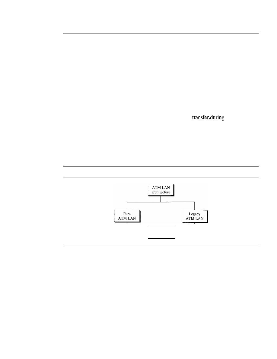
536
CHAPTER
18
VIRTUAL-CIRCUIT NETWORKS: FRAME RELAY AND ATM
18.3
ATM LANs
ATM is mainly a wide-area network (WAN ATM); however, the technology can be
adapted to local-area networks (ATM LANs). The high data rate of the technology (155
and 622 Mbps) has attracted the attention of designers who are looking for greater and
greater speeds in LANs. In addition, ATM technology has several advantages that make
it an ideal LAN:
o
ATM technology supports different types of connections between two end users. It
supports permanent and temporary connections.
o
ATM technology supports multimedia communication with a variety of bandwidths
for different applications. It can guarantee a bandwidth of several megabits per second
for real-time video. It can also provide support for text
off-peak hours.
o
An ATM LAN can be easily adapted for expansion in an organization.
ATM LAN Architecture
Today, we have two ways to incorporate ATM technology in a LAN architecture: creating
a pure ATM LAN or making a legacy ATM LAN. Figure 18.24 shows the taxonomy.
Figure
18.24
ATM LANs
_______
Mixed
architecture
Pure ATM Architecture
In a pure ATM LAN, an ATM switch is used to connect the stations in a LAN, in
exactly the same way stations are connected to an Ethernet switch. Figure 18.25 shows
the situation.
In this way, stations can exchange data at one of two standard rates of ATM tech-
nology (155 and 652 Mbps). However, the station uses a virtual path identifier (VPI)
and a virtual circuit identifier
(Vel),
instead of a source and destination address.
This approach has a major drawback. The system needs to be built from the ground
up; existing LANs cannot be upgraded into pure ATM LANs.
Legacy LAN Architecture
A second approach is to use ATM technology as a backbone to connect traditional
LANs. Figure 18.26 shows this architecture, a legacy ATM LAN.
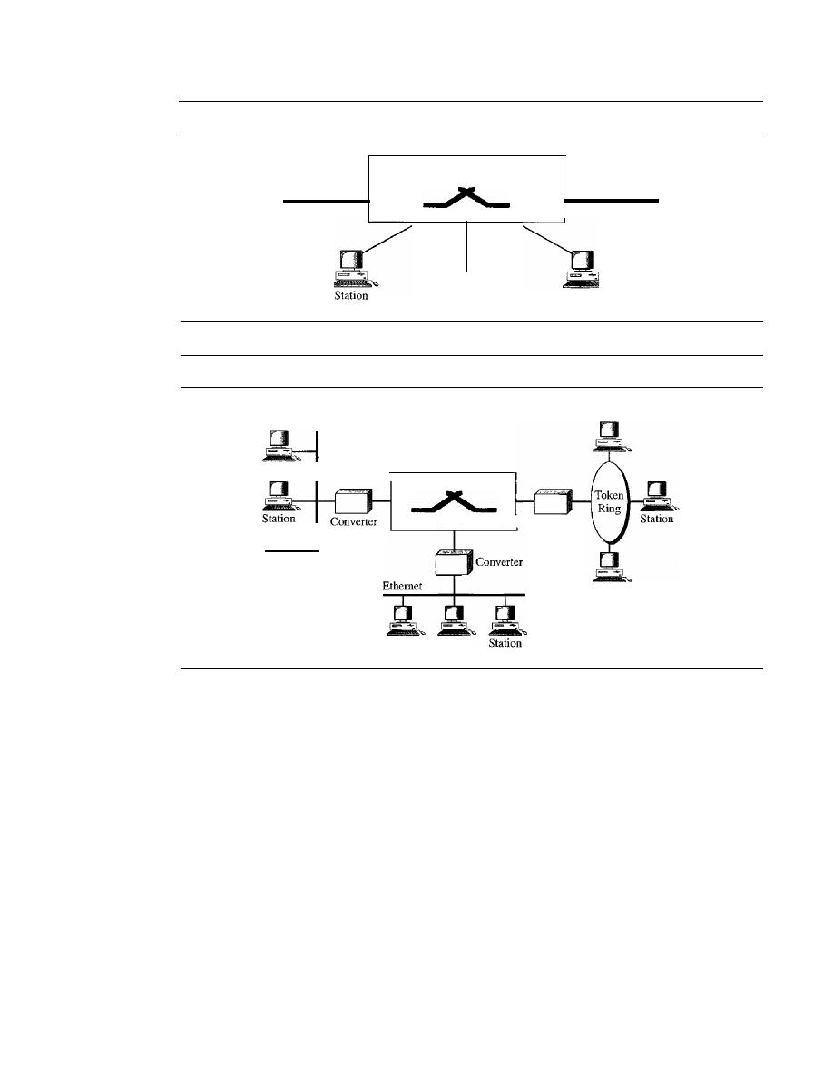
SECTION
18.3
ATM LANs
537
Figure 18.25
Pure ATM LAN
ATM switch
Station
Station
Station
Station
Figure 18.26
Legacy ATM LAN
Station
Station
Converter
ATM switch
Ethernet
Station
Station
Station
Station
In this way, stations on the same LAN can exchange data at the rate and format of
traditional LANs (Ethernet, Token Ring, etc.). But when two stations on two different
LANs need to exchange data, they can go through a converting device that changes the
frame format. The advantage here is that output from several LANs can be multiplexed
together to create a high-data-rate input to the ATM switch. There are several issues
that must be resolved first.
Mixed Architecture
Probably the best solution is to mix the two previous architectures. This means keeping
the existing LANs and, at the same time, allowing new stations to be directly connected
to an ATM switch. The mixed architecture LAN allows the gradual migration of legacy
LANs onto ATM LANs by adding more and more directly connected stations to the
switch. Figure 18.27 shows this architecture.
Again, the stations in one specific LAN can exchange data using the format and
data rate of that particular LAN. The stations directly connected to the ATM switch can
use an ATM frame to exchange data. However, the problem is, How can a station in a
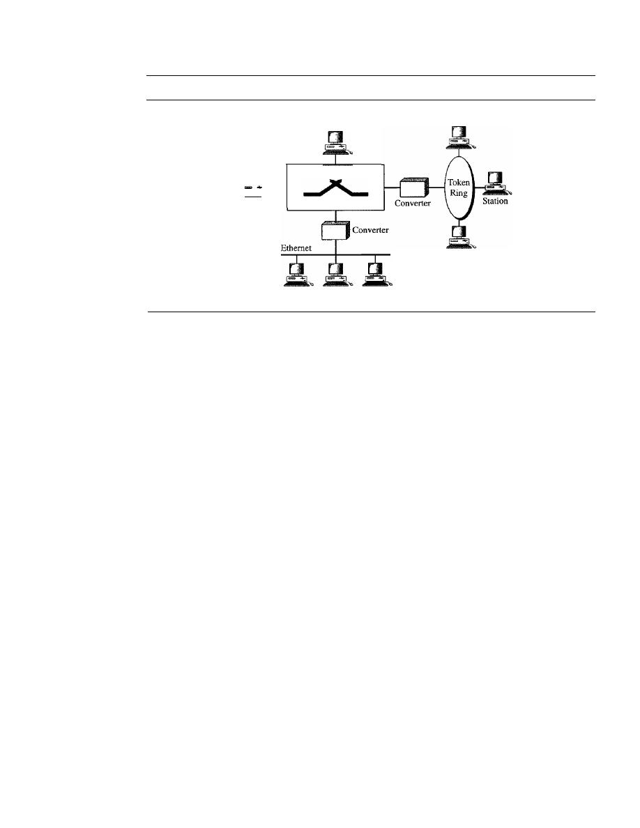
538
CHAPTER
18
VIRTUAL-CIRCUIT NETWORKS: FRAME RELAY AND ATM
Figure 18.27
Mixed architecture ATM IAN
ATM station
ATM station
ATM
switch
Station
Station
Station
Station
Station
traditional LAN communicate with a station directly connected to the ATM switch or
vice versa? We see how the problem is resolved now.
LAN Emulation (LANE)
At the surface level, the use of ATM technology in LANs seems like a good idea. However,
many issues need to be resolved, as summarized below:
o
Connectionless versus connection-oriented. Traditional LANs, such as Ethernet,
are
connectionless protocols.
A station sends data packets to another station when-
ever the packets are ready. There is no
connection establishment
or
connection
termination
phase. On the other hand, ATM is a
connection-oriented protocol;
a
station that wishes to send cells to another station must first establish a connection
and, after all the cells are sent, terminate the connection.
o
Physical addresses versus virtual-circuit identifiers. Closely related to the first
issue is the difference in addressing. A connectionless protocol, such as Ethernet,
defines the route of a packet through
source
and
destination addresses.
However, a
connection-oriented protocol, such as ATM, defines the route of a cell through
virtual connection identifiers (VPIs and VCIs).
o
Multicasting and broadcasting delivery. Traditional LANs, such as Ethernet,
can both
multicast
and
broadcast
packets; a station can send packets to a group
of stations or to all stations. There is no easy way to multicast or broadcast on an
ATM network although point-to-multipoint connections are available.
o
Interoperability. In a mixed architecture, a station connected to a legacy LAN
must be able to communicate with a station directly connected to an ATM switch.
An approach called local-area network emulation (LANE) solves the above-mentioned
problems and allows stations in a mixed architecture to communicate with one another.
The approach uses emulation. Stations can use a connectionless service that emulates a
connection-oriented service. Stations use the source and destination addresses for initial
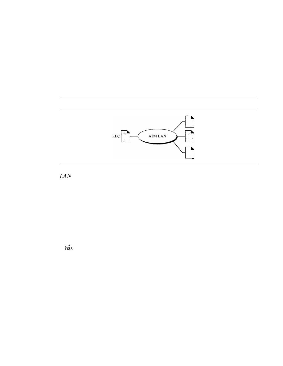
SECTION 18.3
ATM LANs
539
connection and then use VPI and VCI addressing. The approach allows stations to use
unicast, multicast, and broadcast addresses. Finally, the approach converts frames using a
legacy format to ATM cells before they are sent through the switch.
Client/Server Model
LANE is designed as a client/server model to handle the four previously discussed
problems. The protocol uses one type of client and three types of servers, as shown in
Figure 18.28.
Figure 18.28
Client and servers in a LANE
LEes
LES
BUS
Emulation Client
All ATM stations have LAN emulation client (LEC) software installed on top of the
three ATM protocols. The upper-layer protocols are unaware of the existence of the
ATM technology. These protocols send their requests to LEC for a LAN service such as
connectionless delivery using MAC unicast, multicast, or broadcast addresses. The LEC,
however, just interprets the request and passes the result on to the servers.
LAN Emulation Configuration Server
The LAN emulation configuration server (LECS) is used for the initial connection
between the client and LANE. This server is always waiting to receive the initial contact.
It
a well-known ATM address that is known to every client in the system.
LAN Emulation Server
LAN emulation server (LES) software is installed on the LES. When a station
receives a frame to be sent to another station using a physical address, LEC sends a
special frame to the LES. The server creates a virtual circuit between the source and the
destination station. The source station can now use this virtual circuit (and the corre-
sponding identifier) to send the frame or frames to the destination.
Broadcast/Unknown Server
Multicasting and broadcasting require the use of another server called the broadcast!
unknown server (BUS).
If
a station needs to send a frame to a group of stations or to
every station, the frame first goes to the BUS; this server has permanent virtual connec-
tions to every station. The server creates copies of the received frame and sends a copy
to a group of stations or to all stations, simulating a multicasting or broadcasting process.
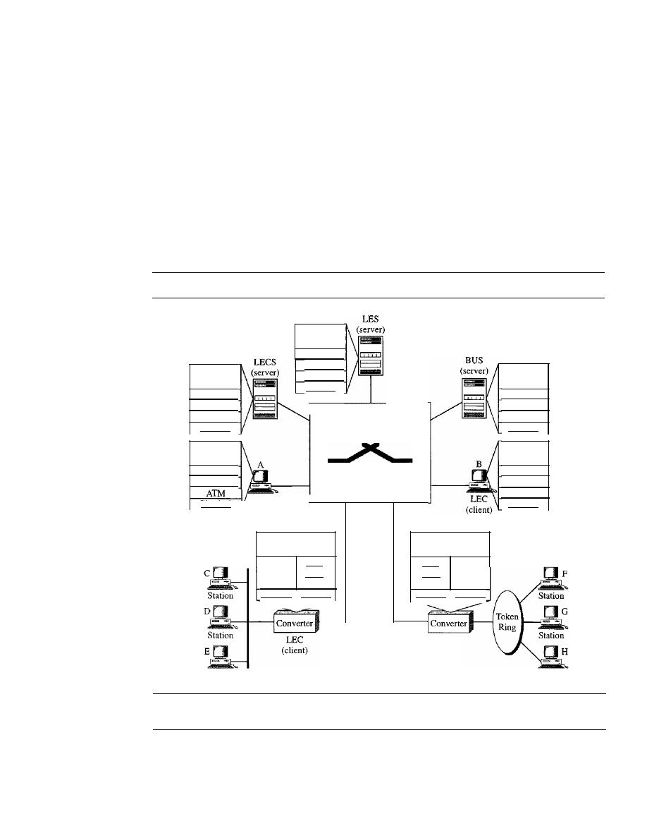
540
CHAPTER
18
ViRTUAL-CIRCUIT NETWORKS: FRAME REIAY AND ATM
The server can also deliver a unicast frame by sending the frame to every station. In this
case the destination address is unknown. This is sometimes more efficient than getting
the connection identifier from the LES.
Mixed Architecture with Client/Server
Figure 18.29 shows clients and servers in a mixed architecture ATM LAN. In the figure,
three types of servers are connected to the ATM switch (they can actually be part of the
switch). Also we show two types of clients. Stations A and B, designed to send and receive
LANE communication, are directly connected to the ATM switch. Stations C, D, E, F, G,
and H in traditional legacy LANs are connected to the switch via a converter. These con-
verters act as LEC clients and communicate on behalf of their connected stations.
Figure 18.29
A mixed architecture ATM IAN using IANE
Upper
layers
ATM
LEC
AAL
ATM
AAL
BUS
Upper
layers
Upper
layers
Physical
Physical
ATM switch
ATM
LES
AAL
Physical
LECS
ATM
AAL
Upper
layers
LEC
AAL
Upper
layers
Physical
LEC
Physical
(client)
Converter
software
Converter
software
LEC
MAC
AAL
ATM
Physical
Physical
LEC
AAL
MAC
ATM
Physical
Physical
LEC
(client)
Station
Station
18.4
RECOMMENDED READING
For more details about subjects discussed in this chapter, we recommend the following
books. The items in brackets [...] refer to the reference list at the end of the text.

SECTION
18.6
SUMMARY
541
Books
Frame Relay and ATM are discussed in Chapter 3 of [Sta98]. ATM LAN is discussed
in Chapter 14 of [For03]. Chapter 7 of [Kei02] also has a good discussion of ATM
LANs.
18.5
KEY TERMS
AALI
AAL2
AAL3/4
AAL5
application adaptation layer (AAL)
Asynchronous Transfer Mode
(ATM)
ATMlayer
ATM switch
backward explicit congestion notification
(BECN)
bandwidth on demand
broadcast/unknown server (BUS)
bursty data
cell
cell network
cell relay
client/server model
congestion control
conyergence sublayer (CS)
data link connection identifier
(DLCI)
discard eligibility (DE)
forward explicit congestion notification
(FECN)
Frame Relay
Frame Relay assembler/disassembler
(FRAD)
LAN emulation client (LEC)
LAN emulation configuration server
(LECS)
LAN emulation server (LES)
legacy ATM LAN
local-area network emulation (LANE)
Local Management Information (LMI)
mixed architecture LAN
network-to-network interface (NNI)
permanent virtual circuit (PVC)
pureATMLAN
quality of service (QoS)
segmentation and reassembly (SAR)
simple and efficient adaptation layer
(SEAL)
switched virtual circuit (SVC)
transmission path (TP)
user-to-network interface (UNI)
virtual circuit (VC)
virtual-circuit identifier (VCl)
virtual path (VP)
virtual path identifier (VPI)
Voice Over Frame Relay (VOFR)
X.25
18.6
SUMMARY
o
Virtual-circuit switching is a data link layer technology in which links are shared.
o
A virtual-circuit identifier (VCI) identifies a frame between two switches.
o
Frame Relay is a relatively high-speed, cost-effective technology that can handle
bursty data.

542
CHAPTER
18
VIRTUAL-CIRCUIT NETWORKS: FRAME RELAY AND ATM
D
Both PVC and SVC connections are used in Frame Relay.
D
The data link connection identifier (DLCI) identifies a virtual circuit in Frame Relay.
o
Asynchronous Transfer Mode (ATM) is a cell relay protocol that, in combination
with SONET, allows high-speed connections.
o
A cell is a small, fixed-size block of information.
D
The ATM data packet is a cell composed of 53 bytes (5 bytes of header and 48 bytes
of payload).
D
ATM eliminates the varying delay times associated with different-size packets.
D
ATM can handle real-time transmission.
o
A user-to-network interface (UNI) is the interface between a user and anATM switch.
o
A network-to-network interface (NNI) is the interface between two ATM switches.
D
In ATM, connection between two endpoints is
through transmission
paths (TPs), virtual paths (VPs), and virtual circuits (VCs).
D
In ATM, a combination of a virtual path identifier (VPI) and a virtual-circuit
identifier identifies a virtual connection.
o
The ATM standard defines three layers:
a. Application adaptation layer (AAL) accepts transmissions from upper-layer
services and maps them into ATM cells.
b. ATM layer provides routing, traffic management, switching, and multiplexing
serVIces.
c. Physical layer defines the transmission medium, bit transmission, encoding, and
electrical-to-optical transformation.
D
TheAAL is divided into two sublayers: convergence sublayer (CS) and segmentation
and reassembly (SAR).
o
There are four different AALs, each for a specific data type:
a. AALI for constant-bit-rate stream.
b. AAL2 for short packets.
c. AAL3/4 for conventional packet switching (virtual-circuit approach or datagram
approach).
d. AAL5 for packets requiring no sequencing and no error control mechanism.
D
ATM technology can be adopted for use in a LAN (ATM LAN).
D
In a pure ATM LAN, an ATM switch connects stations.
D
In a legacy ATM LAN, the backbone that connects traditional LANs uses ATM
technology.
o
A mixed architecture ATM LAN combines features of a pure ATM LAN and a
legacy ATM LAN.
D
Local-area network emulation (LANE) is a client/server model that allows the use
of ATM technology in LANs.
D
LANE software includes LAN emulation client (LECS), LAN emulation configu-
ration server (LECS), LAN emulation server (LES), and broadcast/unknown server
(BUS) modules.
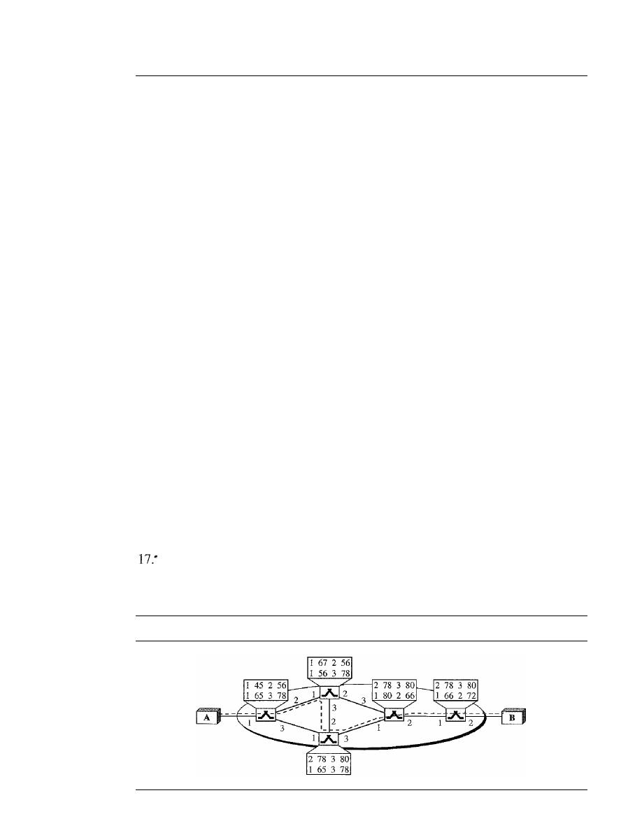
SECTION
18.7
PRACTICE SET
543
18.7
PRACTICE SET
Review Questions
1. There are no sequence numbers in Frame Relay. Why?
2. Can two devices connected to the same Frame Relay network use the same
DLCIs?
3. Why is Frame Relay a better solution for connecting LANs than T-llines?
4. Compare an SVC with a PVc.
5. Discuss the Frame Relay physical layer.
6. Why is multiplexing more efficient if all the data units are the same size?
7. How does an NNI differ from a UNI?
8. What is the relationship between TPs, VPs, and VCs?
9. How is an ATM virtual connection identified?
10. Name the ATM layers and their functions.
11. How many virtual connections can be defined in a UNI? How many virtual connec-
tions can be defined in an NNI?
12. Briefly describe the issues involved in using ATM technology in LANs.
Exercises
13. The address field of a Frame Relay frame is 1011000000010111. What is the DLCI
(in decimal)?
14. The address field of a Frame Relay frame is 101100000101001. Is this valid?
15. Find the DLCI value if the first 3 bytes received is 7C 74 El in hexadecimal.
16. Find the value of the 2-byte address field in hexadecimal if the DLCI is 178.
Assume no congestion.
In
Figure 18.30 a virtual connection is established between A and B. Show the
DLCI for each link.
Figure 18.30
Exercise 17
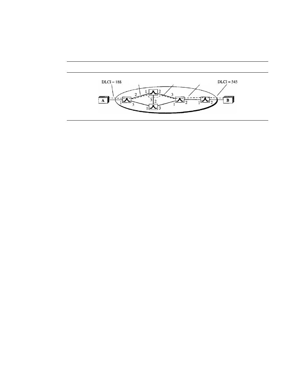
544
CHAPTER 18
VIRTUAL-CIRCUIT NETWORKS: FRAME RELAY ANDATM
18. In Figure 18.31 a virtual connection is established between A and B. Show the
corresponding entries in the tables of each switch.
Figure 18.31
Exercise 18
DLCI= 233
DLCI = 11 1
DLCI = 99
19. An AALllayer receives data at 2 Mbps. How many cells are created per second by
the ATM layer?
20. What is the total efficiency of ATM using AAL1 (the ratio of received bits to sent
bits)?
21.
If
an application uses AAL3/4 and there are 47,787 bytes of data coming into the
CS, how many padding bytes are necessary? How many data units get passed from
the SAR to the ATM layer? How many cells are produced?
22. Assuming no padding, does the efficiency of ATM using AAL3/4 depend on the size
of the packet? Explain your answer.
23. What is the minimum number of cells resulting from an input packet in the AAL3/4
layer? What is the maximum number of cells resulting from an input packet?
24. What is the minimum number of cells resulting from an input packet in the AAL5
layer? What is the maximum number of cells resulting from an input packet?
25. Explain why padding is unnecessary in AAL1, but necessary in other AALs.
26. Using AAL3/4, show the situation where we need
of padding.
a. 0 bytes (no padding)
b. 40 bytes
c. 43 bytes
27. UsingAAL5, show the situation where we need
of padding.
a. 0 bytes (no padding)
b. 40 bytes
c. 47 bytes
28. In a 53-byte cell, how many bytes belong to the user in the following (assume no
padding)?
a. AALI
b. AAL2
c. AAL3/4 (not the first or last cell)
d. AAL5 (not the first or last cell)

SECTION 18.7
PRACTICE SET
545
Research Activities
29. Find out about 1.150 protocol that provides generic flow control for UNI interface.
30. ATM uses the 8-bit
HEe
(header error control) field to control errors in the first four
bytes (32 bits) of the header. The generating polynomial is
x
8
+
x
2
+
X
+
1. Find out
how this is done.
31.
Find the format of the LANE frames and compare it with the format of the Ethernet
frame.
32. Find out about different steps involved in the operation of a LANE.


Network Layer
Objectives
The network layer is responsible for the source-to-destination delivery of a packet, possi-
bly across multiple networks (links). Whereas the data link layer oversees the delivery of
the packet between two systems on the same network (links), the network layer ensures
that each packet gets from its point of origin to its final destination.
The network layer is responsible for the delivery of individual
packets from the source to the destination host.
The network layer adds a header that includes the logical addresses of the sender
and receiver to the packet corning from the upper layer.
If
a packet travels through the
Internet, we need this addressing system to help distinguish the source and destination.
When independent networks or links are connected together to create an internet-
work, routers or switches route packets to their final destination. One of the functions
of the network layer is to provide a routing mechanism.
In Part 4 of the book, we first discuss logical addressing (referred to as IP addressing
in the Internet). We then discuss the main as well as some auxiliary protocols that are
for controlling the delivery of a packet from its source to its destination.
Part 4 of the book is devoted to the network layer and
the services provided by this layer.
Chapters
This part consists of four chapters: Chapters 19 to 22.
Chapter 19
Chapter 19 discusses logical or IP addressing. We first discuss the historical classful
addressing. We then describe the new classless addressing designed to alleviate some
problems inherent in classful addressing. The completely new addressing system, IPv6,
which may become prevalent in the near future, is also discussed.

Chapter 20
Chapter 20 is devoted to the main protocol at the network layer that supervises and con-
trols the delivery of packets from the source to destination. This protocol is called the
Internet Protocol or IP.
Chapter 21
Chapter 21 is devoted to some auxiliary protocols defined at the network layer, that
help the IP protocol do its job. These protocols perform address mapping (logical to
physical or vice versa), error reporting, and facilitate multicast delivery.
Chapter 22
Delivery and routing of packets in the Internet is a very
and important issue.
We devote Chapter 22 to this matter. We first discuss the mechanism of delivery and
routing. We then briefly discuss some unicast and multicast routing protocols used in
the Internet today.

CHAPTER 19
Network Layer:
Logical Addressing
As we discussed in Chapter 2, communication at the network layer is
(computer-to-computer); a computer somewhere in the world needs to communicate
with another computer somewhere else in the world. Usually, computers communicate
through the Internet. The packet transmitted by the sending computer may pass through
several LANs or WANs before reaching the destination computer.
For this level of communication, we need a global addressing scheme; we called
this logical addressing in Chapter 2. Today, we use the term IP address to mean a logical
address in the network layer of the TCP/IP protocol suite.
The Internet addresses are 32 bits in length; this gives us a maximum of 2
32
addresses. These addresses are referred to as IPv4 (IP version 4) addresses or simply IP
addresses if there is no confusion.
The need for more addresses, in addition to other concerns about the IP layer,
vated a new design of the IP layer called the new generation of IP or IPv6 (lP version 6).
In this version, the Internet uses 128-bit addresses that give much greater flexibility in
address allocation. These addresses are referred to as IPv6 (IP version 6) addresses.
In this chapter, we first discuss IPv4 addresses, which are currently being used in the
Internet. We then discuss the IPv6 addresses, which may become dominant in the future.
19.1
IPv4 ADDRESSES
An IPv4 address is a 32-bit address that uniquely and universally defines the connection
of a device (for example, a computer or a router) to the Internet.
An IPv4 address is 32 bits long.
IPv4 addresses are unique. They are unique in the sense that each address defines
one, and only one, connection to the Internet. Two devices on the Internet can never
have the same address at the same time. We will see later that, by using some strategies,
an address may be assigned to a device for a time period and then taken away and
assigned to another device.
549

550
CHAPTER
19
NETWORK IAYER: LOGICAL ADDRESSING
On the other hand, if a device operating at the network layer has
m
connections to
the Internet, it needs to have
m
addresses. We will see later that a router is such a
device.
The IPv4 addresses are universal in the sense that the addressing system must be
accepted by any host that wants to be connected to the Internet.
The IPv4 addresses are unique and universal.
Address Space
A protocol such as IPv4 that defines addresses has an
address space.
An address space
is the total number of addresses used by the protocol.
If
a protocol uses
N
bits to define
an address, the address space is
2
N
because each bit can have two different values (0 or 1)
and
N bits can have 2
N
values.
IPv4 uses 32-bit addresses, which means that the address space is 2
32
or
4,294,967,296 (more than 4 billion). This means that, theoretically, if there were no
restrictions, more than 4 billion devices could be connected to the Internet. We will see
shortly that the actual number is much less because of the restrictions imposed on the
addresses.
The address space of IPv4 is 2
32
or 4,294,967,296.
Notations
There are two prevalent notations to show an IPv4 address:
binary notation and dotted-
decimal notation.
Binary Notation
In binary notation, the IPv4 address is displayed as 32 bits. Each octet is often referred
to as a byte. So it is common to hear an IPv4 address referred to as a 32-bit address or a
4-byte address. The following is
an
example of an IPv4 address in binary notation:
01110101 10010101 00011101 00000010
Dotted-Decimal Notation
To make the IPv4 address more compact and easier to read, Internet addresses are usu-
ally written in decimal form with a decimal point (dot) separating the bytes. The fol-
lowing is the
notation of the above address:
117.149.29.2
Figure 19.1 shows an IPv4 address in both binary and dotted-decimal notation.
Note that because each byte (octet) is 8 bits, each number in dotted-decimal notation is
a value ranging from 0 to 255.
SECTION
19.1
IPv4 ADDRESSES
551
Figure 19.1
Dotted-decimal notation and
notation for an IPv4 address
10000000
0000 10 II
00000011
00011111
128.11.3.31
Numbering systems are reviewed
in Appendix B.
Example 19.1
Change the following IPv4 addresses from binary notation to dotted-decimal notation.
a. 10000001 00001011
00001011 11101111
b. 11000001 10000011
00011011 11111111
Solution
We replace each group of 8 bits with its equivalent decimal number (see Appendix B) and add
dots for separation.
a. 129.11.11.239
b. 193.131.27.255
Example 19.2
Change the following IPv4 addresses from dotted-decimal notation to binary notation.
a. 111.56.45.78
b. 221.34.7.82
Solution
We replace each decimal number with its binary equivalent (see Appendix B).
a.• 01101111 00111000 00101101 01001110
b. 11011101 00100010 00000111 01010010
Example 19.3
Find the error, if any, in the following IPv4 addresses.
a. 111.56.045.78
b. 221.34.7.8.20
c. 75.45.301.14
d. 11100010.23.14.67
Solution
a. There must be no leading zero (045).
b. There can be no more than four numbers in an IPv4 address.
c. Each number needs to be less than or equal to 255 (301 is outside this range).
d. A mixture of binary notation and dotted-decimal notation is not allowed.
552
CHAPTER
19
NETWORK LAYER: LOGICAL ADDRESSING
Classful Addressing
IPv4 addressing, at its inception, used the concept of classes. This architecture is called
classful addressing. Although this scheme is becoming obsolete, we briefly discuss it
here to show the rationale behind classless addressing.
In classful addressing, the address space is divided into five classes: A, B, C, D,
and E. Each class occupies some part of the address space.
In
classful addressing, the address space is divided into five classes:
A, B, C, D, and E.
We can find the class of an address when given the address in binary notation
or dotted-decimal notation.
If
the address is given in binary notation, the first few
bits can immediately tell us the class of the address.
If
the address is given in
decimal-dotted notation, the first byte defines the class. Both methods are shown in
Figure 19.2.
Figure 19.2
Finding the classes in binary and dotted-decimal notation
First
Second
Third
Fourth
First
Second
Third
Fourth
byte
byte
byte
byte
byte
byte
byte
byte
Class A
0
II
II
II
Class A
I
0-127
II
II
II
Class B
10
II
II
II
Class B
1128-19111
II
II
Class C
110
II
II
II
Class C
1192-22311
II
II
Class D
1110
II
II
II
Class D
1224--23911
II
II
Class E
1111
II
II
II
Class E
1240-25511
II
II
a. Binary notation
b. Dotted-decimal notation
Example 19.4
Find the class of each address.
a.
00000001 00001011 00001011 11101111
b.
11000001 10000011 00011011 11111111
c.
14.23.120.8
d.
252.5.15.111
Solution
a. The first bit is O. This is a class A address.
b. The first 2 bits are 1; the third bit is O. This is a class C address.
c. The first byte is 14 (between 0 and 127); the class is
A.
d. The first byte is 252 (between 240 and 255); the class is E.
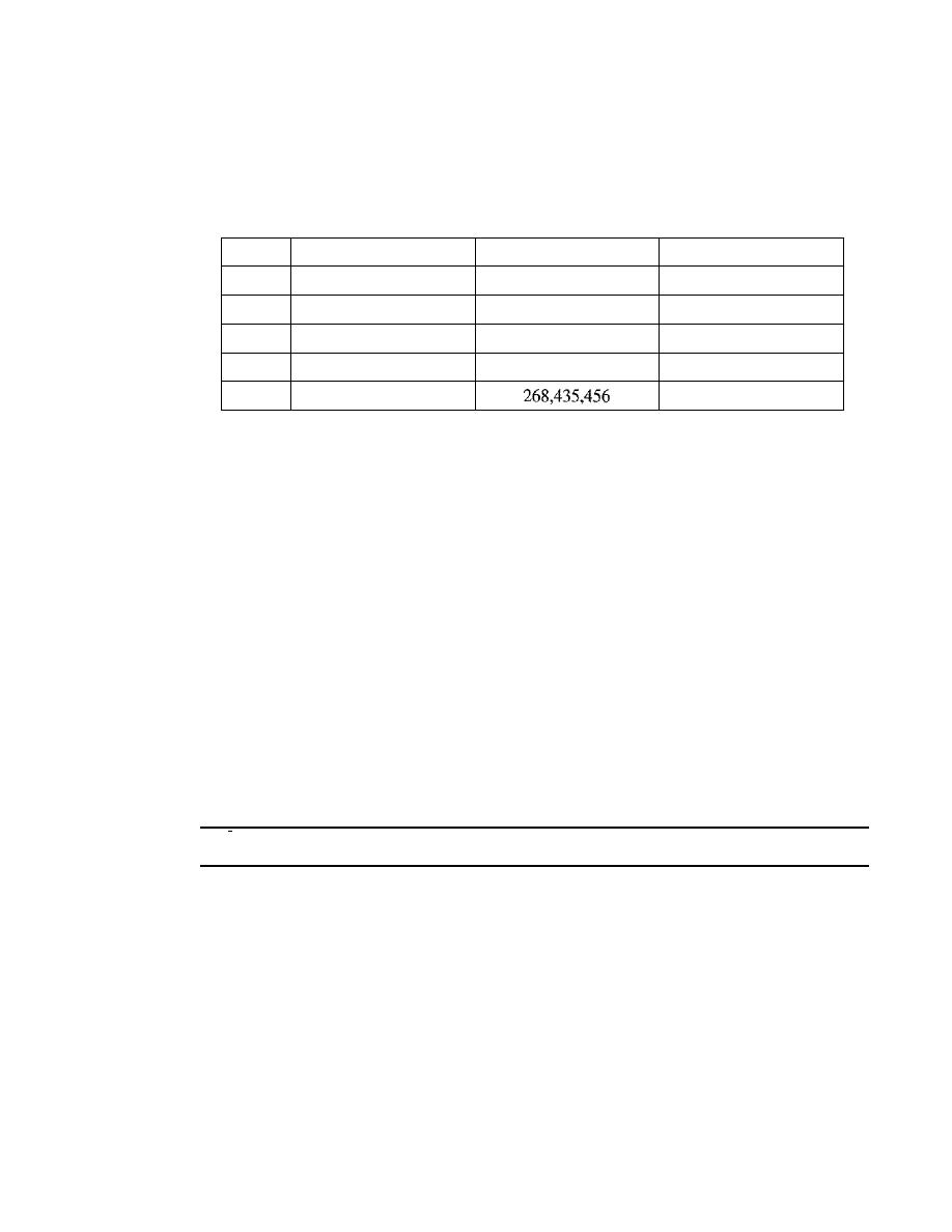
SECTION
19.1
IPv4 ADDRESSES
553
Classes and Blocks
One problem with classful addressing is that each class is divided into a fixed number
of blocks with each block having a fixed size as shown in Table 19.1.
Table 19.1
Number of blocks and block size in classfulIPv4 addressing
Class
Number ofBlocks
Block Size
Application
A
128
16,777,216
Unicast
B
16,384
65,536
Unicast
C
2,097,152
256
Unicast
D
1
268,435,456
Multicast
E
1
Reserved
Let us examine the table. Previously, when an organization requested a block of
addresses, it was granted one in class A, B, or
C.
Class A addresses were designed for
large organizations with a large number of attached hosts or routers. Class B addresses
were designed for midsize organizations with tens of thousands of attached hosts or
routers. Class C addresses were designed for small organizations with a small number of
attached hosts or routers.
We can see the flaw in this design. A block in class A address is too large for
almost any organization. This means most of the addresses in class A were wasted and
were not used. A block in class B is also very large, probably too large for many of the
organizations that received a class B block. A block in class C is probably too small for
many organizations. Class D addresses were designed for multicasting as we will see in
a later chapter. Each address in this class is used to define one group of hosts on the
Internet. The Internet authorities wrongly predicted a need for 268,435,456 groups.
This never happened and many addresses were wasted here too. And lastly, the class E
addresses were reserved for future use; only a few were used, resulting in another waste
of addresses.
«
In c1assfnl addressing, a large part of the available addresses were wasted.
Netid and Hostid
In classful addressing, an IP address in class
A,
B, or C is divided into netid and hostid.
These parts are of varying lengths, depending on the class of the address. Figure 19.2
shows some netid and hostid bytes. The netid is in color, the hostid is in white. Note that
the concept does not apply to classes D and E.
In class A, one byte defines the netid and three bytes define the hostid. In class B,
two bytes define the netid and two bytes define the hostid. In class C, three bytes define
the netid and one byte defines the hostid.
Mask
Although the length of the netid and hostid (in bits) is predetermined in classful address-
ing, we can also use a mask (also called the default mask), a 32-bit number made of
554
CHAPTER
19
NETWORK lAYER: LOG1CALADDRESSING
contiguous Is followed by contiguous as. The masks for classes A, B, and C are shown
in Table 19.2. The concept does not apply to classes D and
E.
Table 19.2
Default masks for classful addressing
Class
Binary
Dotted-Decimal
CIDR
A
11111111 00000000 00000000 00000000
255.0.0.0
18
B
11111111 11111111 00000000 00000000
255.255.0.0
116
C
11111111 11111111 11111111 00000000
255.255.255.0
124
The mask can help us to find the netid and the hostid. For example, the mask for a
class A address has eight 1s, which means the first 8 bits of any address in class A
define the
the next 24 bits define the hostid.
The last column of Table 19.2 shows the mask in the form In where n can be 8, 16,
or 24 in classful addressing. This notation is also called slash notation or
Classless
Interdomain Routing (CIDR)
notation. The notation is used in classless addressing,
which we will discuss later. We introduce it here because it can also be applied to class-
ful addressing. We will show later that classful addressing is a special case of classless
addressing.
Subnetting
During the era of classful addressing,
subnetting
was introduced.
If
an organization was
granted a large block in class A or B, it could divide the addresses into several contiguous
groups and assign each group to smaller networks (called
subnets)
or, in rare cases,
share part of the addresses with neighbors. Subnetting increases the number of Is in the
mask, as we will see later when we discuss classless addressing.
Supernetting
The time came when most of the class A and class B addresses were depleted; however,
there was still a huge demand for midsize blocks. The size of a class C block with a
maximum number of 256 addresses did not satisfy the needs of most organizations.
Even a midsize organization needed more addresses. One solution was
supernetting.
In supernetting, an organization can combine several class C blocks to create a larger
range of addresses. In other words, several networks are combined to create a super-
network or a
supemet.
An organization can apply for a set of class C blocks instead of
just one. For example, an organization that needs 1000 addresses can be granted four
contiguous class C blocks. The organization can then use these addresses to create one
supernetwork. Supernetting decreases the number of Is in the mask. For example, if an
organization is given four class C addresses, the mask changes from /24 to /22. We will
see that classless addressing eliminated the need for supernetting.
Address Depletion
The flaws in classful addressing scheme combined with the fast growth of the Internet led
to the near depletion of the available addresses. Yet the number of devices on the Internet
is much less than the 2
32
address space. We have run out of class A and B addresses, and
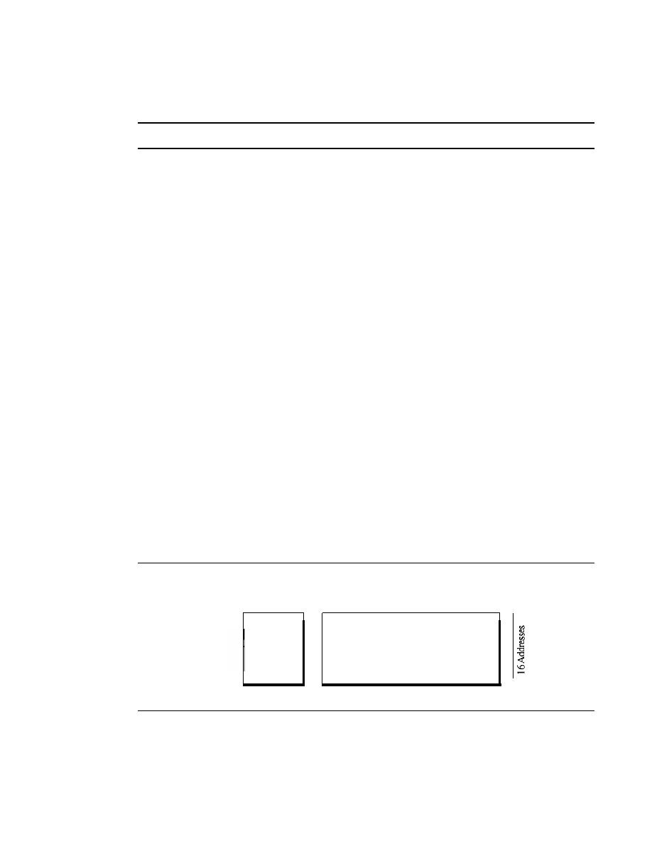
SECTION
19.1
IPv4ADDRESSES
555
a class C block is too small for most midsize organizations. One solution that has
alleviated the problem is the idea of classless addressing.
Classful addressing, which is almost obsolete, is replaced with classless addressing.
Classless Addressing
To overcome address depletion and give more organizations access to the Internet,
classless addressing was designed and implemented. In this scheme, there are no
classes, but the addresses are still granted in blocks.
Address Blocks
In classless addressing, when an entity, small or large, needs to be connected to the
Internet,
it
is granted a block (range) of addresses. The size of the block (the number of
addresses) varies based on the nature and size of the entity. For example, a household
may be given only two addresses; a large organization may be given thousands of
addresses. An
ISP,
as the Internet service provider, may be given thousands or hundreds
of thousands based on the number of customers it may serve.
Restriction
To simplify the handling of addresses, the Internet authorities impose
three restrictions on classless address blocks:
1. The addresses in a block must be contiguous, one after another.
2. The number of addresses in a block must be a power of 2 (I, 2, 4, 8, ... ).
3. The first address must be evenly divisible by the number of addresses.
Example 19.5
Figure 19.3 shows a block of addresses, in both binary and dotted-decimal notation, granted to a
small business that needs 16 addresses.
Figure 19.3
A block of
16
addresses granted to a small organization
Block
Block
-
First
205.16.37.32
11001101
00010000
00100101
00100000
205.16.37.33
11001101
00010000
00100101
00100001
Last
205.16.37.47
11001101
00010000
00100101
00101111
1 -
a. Decimal
b. Binary
We can see that the restrictions are applied to this block. The addresses are contiguous.
The number of addresses is a power of 2 (16
=
2
4
),
and the first address is divisible by 16. The
first address, when converted to a decimal number, is 3,440,387,360, which when divided by
16 results in 215,024,210. In Appendix B, we show how to find the decimal value of an
IP address.

556
CHAPTER
19
NETWORK LAYER: LOGICAL ADDRESSING
Mask
A better way to define a block of addresses is to select any address in the block and the
mask. As we discussed before, a mask is a 32-bit number in which the
n
leftmost bits
are Is and the 32 -
n
rightmost bits are Os. However, in classless addressing the mask
for a block can take any value from 0 to 32. It is very convenient to give just the value
of
n
preceded by a slash (CIDR notation).
In 1Pv4 addressing, a block of addresses can be defined as
x.y.z.tln
in which x.y.z.t defines one of the addresses and the
In defines the mask.
The address and the
In
notation completely define the whole block (the first
address, the last address, and the number of addresses).
First Address
The first address in the block can be found by setting the 32 - n right-
most bits in the binary notation of the address to Os.
The first address in the block can be found by setting the rightmost 32 -
n bits to Os.
Example 19.6
A block of addresses is granted to a small organization. We know that one of the addresses is
205.16.37.39/28.
What is the first address in the block?
Solution
The binary representation of the given address is 11001101 00010000 00100101 00100 I 11. If we
set 32 - 28 rightmost bits to 0, we get 11001101 000100000100101 0010000 or 205.16.37.32.
This is actually the block shown in Figure 19.3.
Last Address
The last address in the block can be found by setting the 32 - n right-
most bits in the binary notation of the address to Is.
The last address in the block can be found by setting the rightmost 32 -
n bits to Is.
Example 19.7
Find the last address for the block in Example 19.6.
Solution
The binary representation of the given address is 11001101 000100000010010100100111. If we
set 32 - 28 rightmost bits to 1, we get 11001101 00010000 001001010010
1111
or 205.16.37.47.
This is actually the block shown in Figure 19.3.
Number of Addresses
The number of addresses in the block is the difference between
the last and first address.
It
can easily be found using the formula 2
32
-
n
.
The number of addresses in the block can be found by using the formula
2
32
-
n
•

SECTION
19.1
IPv4ADDRESSES
557
Example 19.8
Find the number of addresses in Example 19.6.
Solution
The value of n is 28, which means that number of addresses is 2
32
-
28
or 16.
Example 19.9
Another way to find the first address, the last address, and the number of addresses is to represent
the mask as a 32-bit binary (or 8-digit hexadecimal) number. This is particularly useful when we
are writing a program to find these pieces of information.
In
Example 19.5 the /28 can be repre-
sented as 11111111 11111111 11111111 11110000 (twenty-eight Is and four Os). Find
a. The first address
h. The last address
c. The number of addresses
Solution
a. The first address can be found by ANDing the given addresses with the mask. ANDing here is
done bit by bit. The result of ANDing 2 bits is 1 if both bits are Is; the result is 0 otherwise.
Address:
First address:
11001101 00010000 00100101 00100111
11111111 11111111 11111111 11110000
11001101 00010000 00100101 00100000
b. The last address can be found by ORing the given addresses with the complement of the
mask. ORing here is done bit by bit. The result of ORing 2 bits is 0 if both bits are Os; the
result is 1 otherwise. The complement of a number is found by changing each 1 to 0 and
each 0 to 1.
Address:
Mask complement:
Last address:
11001101 00010000 00100101 00100111
00000000 00000000 00000000 00001111
11001101 00010000
00100101 00101111
c. The number of addresses can be found by complementing the mask, interpreting it as a
decimal number, and adding 1 to it.
Mask complement:
Number of addresses:
000000000 00000000 00000000 00001111
15
+
1
=
16
Network Addresses
A very important concept in IP addressing is the
network address.
When an organiza-
tion is given a block of addresses, the organization is free to allocate the addresses to
the devices that need to be connected to the Internet. The first address in the class, how-
ever, is normally (not always) treated as a special address. The first address is called the
network address and defines the organization network. It defines the organization itself
to the rest of the world. In a later chapter we will see that the first address is the one that
is used by routers to direct the message sent to the organization from the outside.
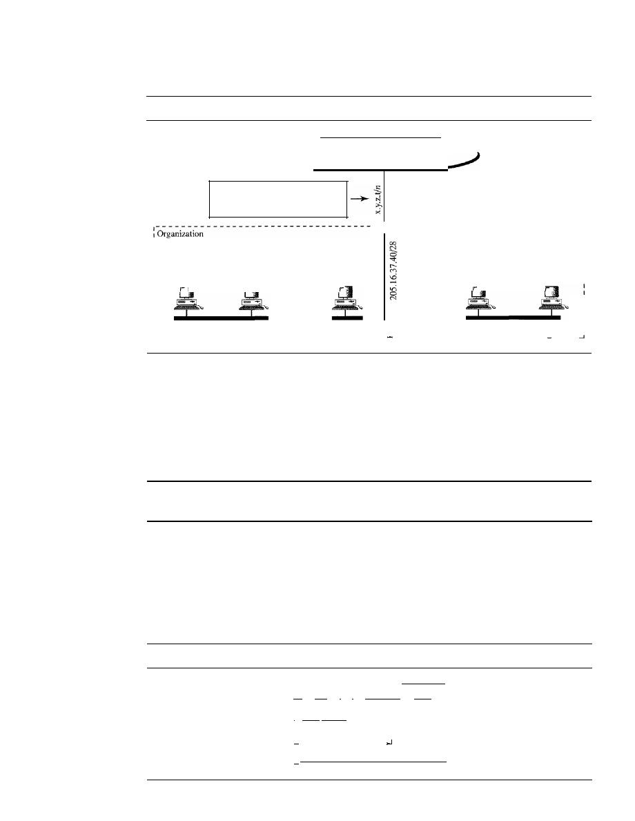
558
CHAPTER
19
NETWORK LAYER: LOGICAL ADDRESSING
Figure 19.4 shows an organization that is granted a 16-address block.
Figure 19.4
A network configuration for the block 205.16.37.32/28
Rest of
the Internet
All messages with receiver addresses
205.16.37.32 to 205.16.37.47
are routed to x.y.z.t/n
-----------------------------1
1
1
I
1
1
1
1
205.16.37.46/28
205.16.37.47/28
1
1
1
1
1
1
1
:
network
I
I
I
I
1205.16.37.33/28 205.16.37.34/28
205.16.37.39/28
:
I
I
I
I
: Network address:
205.16.37.32/28
L
The organization network is connected to the Internet via a router. The router has
two addresses. One belongs to the granted block; the other belongs to the network that
is at the other side of the router. We call the second address
x.y.z.t/n
because we do not
know anything about the network it is connected to at the other side. All messages des-
tined for addresses in the organization block (205.16.37.32 to 205.16.37.47) are sent,
directly or indirectly, to
x.y.z.t/n.
We say directly or indirectly because we do not know
the structure of the network to which the other side of the router is connected.
The first address in a block is normally not assigned to any device; it is used as the
network address that represents the organization to the rest of the world.
Hierarchy
IP addresses, like other addresses or identifiers we encounter these days, have levels of
hierarchy. For example, a telephone network in North America has three levels of hier-
archy. The leftmost three digits define the area code, the next three digits define the
exchange, the last four digits define the connection of the local loop to the central
office. Figure 19.5 shows the structure of a hierarchical telephone number.
Figure 19.5
Hierarchy in a telephone network in North America
(I
408
I)I
8641-1
8902
1
I
: Area code:
I
I
Exchange office
It
I
I
Subscriber
It

SECTION
19.1
IPv4ADDRESSES
559
Two-Level Hierarchy: No Subnetting
An IP address can define only two levels of hierarchy when not subnetted. The
n left-
most bits of the address x.y.z.tJn define the network (organization network); the 32 - n
rightmost bits define the particular host (computer or router) to the network. The two
common terms are prefix and suffix. The part of the address that defines the network is
called the prefix; the part that defines the host is called the suffix. Figure 19.6 shows
the hierarchical structure of an IPv4 address.
Figure 19.6
Two levels of hierarchy in an IPv4 address
28 bits
4 bits
I
I
I
I
Network prefix
I
I
I
I
I
I
Host address
I
,
)1
The prefix is common to all addresses in the network; the suffix changes from one
device to another.
Each address in the block can be considered as a two-level hierarchical structure:
the leftmost
n bits (prefix) define the network;
the rightmost 32 -
n
bits define the host.
Three-Levels of Hierarchy: Subnetting
An organization that is granted a large block of addresses may want to create clusters of
networks (called subnets) and divide the addresses between the different subnets. The
rest of the world still sees the organization as one entity; however, internally there are
several subnets. All messages are sent to the router address that connects the organization
to the rest of the Internet; the router routes the message to the appropriate subnets. The
organization, however, needs to create small subblocks of addresses, each assigned to
specific subnets. The organization has its own mask; each subnet must also have its own.
As an example, suppose an organization is given the block 17.12.40.0/26, which
contains 64 addresses. The organization has three offices and needs to divide the
addresses into three subblocks of 32, 16, and 16 addresses. We can find the new masks
by using the following arguments:
1. Suppose the mask for the first subnet is n1, then 2
32
-
n1
must be 32, which means
that n1
=
27.
2. Suppose the mask for the second subnet is n2, then 2
32
-
n2
must be 16, which
means that n2
=
28.
3. Suppose the mask for the third subnet is n3, then 2
32
-
n3
must be 16, which means
that n3
=
28.
This means that we have the masks 27, 28, 28 with the organization mask being 26.
Figure 19.7 shows one configuration for the above scenario.
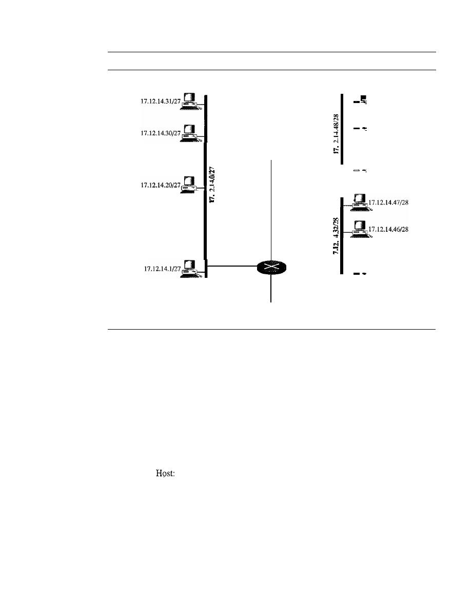
560
CHAPTER
19
NETWORK LAYER: LOGICAL ADDRESSING
Figure 19.7
Configuration and addresses in a subnetted network
,------------------------------------------------------------1
Subnet 1
Subnet 3
:
17.12.14.63/28 :
I
1
1
1
17.12.14.62/28
1
I
17.12.14.50/28
17.12.14.49/28
Subnet 2
-
17.12.14.34/28
17.12.14.33128
17.12.14.2127
-
··
•
Network: 17.12.14.11/26
x.y.z.tln
To the rest of
the Internet
Let us check to see if we can find the subnet addresses from one of the addresses in
the subnet.
a. In subnet 1, the address 17.12.14.29/27 can give us the subnet address if we use the
mask /27 because
Host:
Mask:
Subnet:
00010001 00001100 00001110 00011101
/27
00010001 00001100 00001110 00000000 .... (17.12.14.0)
b. In subnet 2, the address 17.12.14.45/28 can give us the subnet address if we use the
mask /28 because
00010001 00001100 00001110 00101101
Mask:
/28
Subnet:
00010001 00001100 00001110 00100000 .... (17.12.14.32)
c. In subnet 3, the address 17.12.14.50/28 can give us the subnet address if we use the
mask /28 because
Host:
00010001 00001100 00001110 00110010
Mask:
/28
Subnet:
00010001 00001100 00001110 00110000 .... (17.12.14.48)
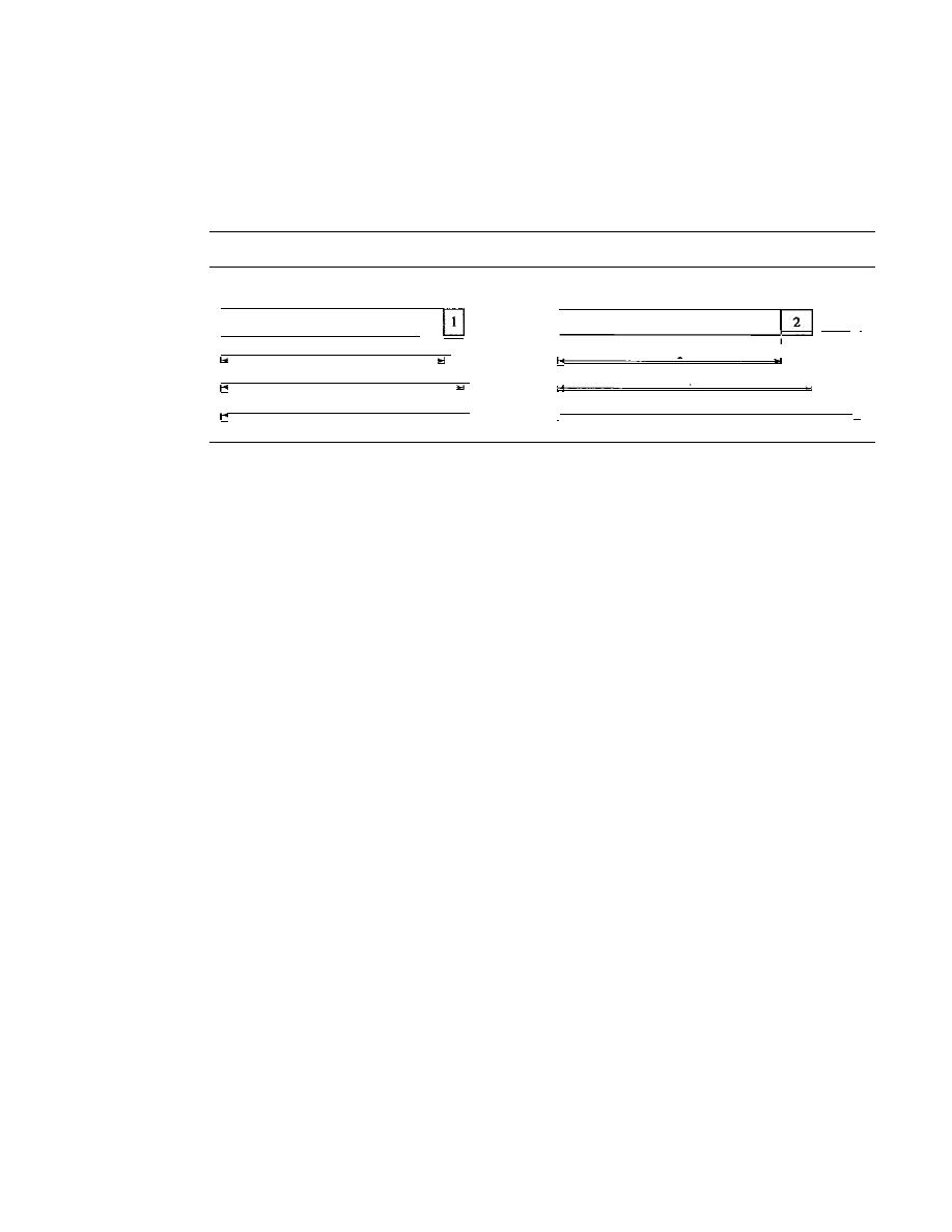
SECTION 19.1
IPv4 ADDRESSES
561
Note that applying the mask of the network,
126,
to any of the addresses gives us the
network address 17.12.14.0/26. We leave this proof to the reader.
We can say that through subnetting, we have three levels of hierarchy. Note that in
our example, the subnet prefix length can differ for the subnets as shown in Figure 19.8.
Figure 19.8
Three-level hierarchy in an IPv4 address
II
Host address
Subnets
2 and 3
26 bits
4bits
I
I
I
Network prefix
I
I
I
I
I
I
I
Subnet prefix
I
I
I
I
I
Subnet 1
26 bits
5 bits
I
I
I
I
I
Network prefix
I
I
I
I
I
I
I
I
Subnet prefix
I
I
t
I
I
I
Host address
I
I
More Levels of Hierarchy
The structure of classless addressing does not restrict the number of hierarchical levels.
An organization can divide the granted block of addresses into subblocks. Each sub-
block can in turn be divided into smaller subblocks. And so on. One example of this is
seen in the ISPs. A national ISP can divide a granted large block into smaller blocks
and assign each of them to a regional ISP. A regional ISP can divide the block received
from the national ISP into smaller blocks and assign each one to a local ISP. A local ISP
can divide the block received from the regional ISP into smaller blocks and assign each
one to a different organization. Finally, an organization can divide the received block
and make several subnets out of it.
Address Allocation
The next issue in classless addressing is address allocation. How are the blocks allocated?
The ultimate responsibility of address allocation is given to a global authority called the
Internet Corporation for Assigned Names and Addresses (ICANN). However, ICANN
does not normally allocate addresses to individual organizations. It assigns a large block
of addresses to an ISP. Each ISP, in turn, divides its assigned block into smaller subblocks
and grants the subblocks to its customers. In other words, an ISP receives one large block
to be distributed to its Internet users. This is called address aggregation: many blocks of
addresses are aggregated in one block and granted to one ISP.
Example 19.10
An ISP is granted a block of addresses starting with 190.100.0.0/16 (65,536 addresses). The ISP
needs to distribute these addresses to three groups of customers as follows:
a. The first group has 64 customers; each needs 256 addresses.
b. The second group has 128 customers; each needs 128 addresses.
c. The third group has 128 customers; each needs 64 addresses.
Design the subblocks and find out how many addresses are still available after these allocations.
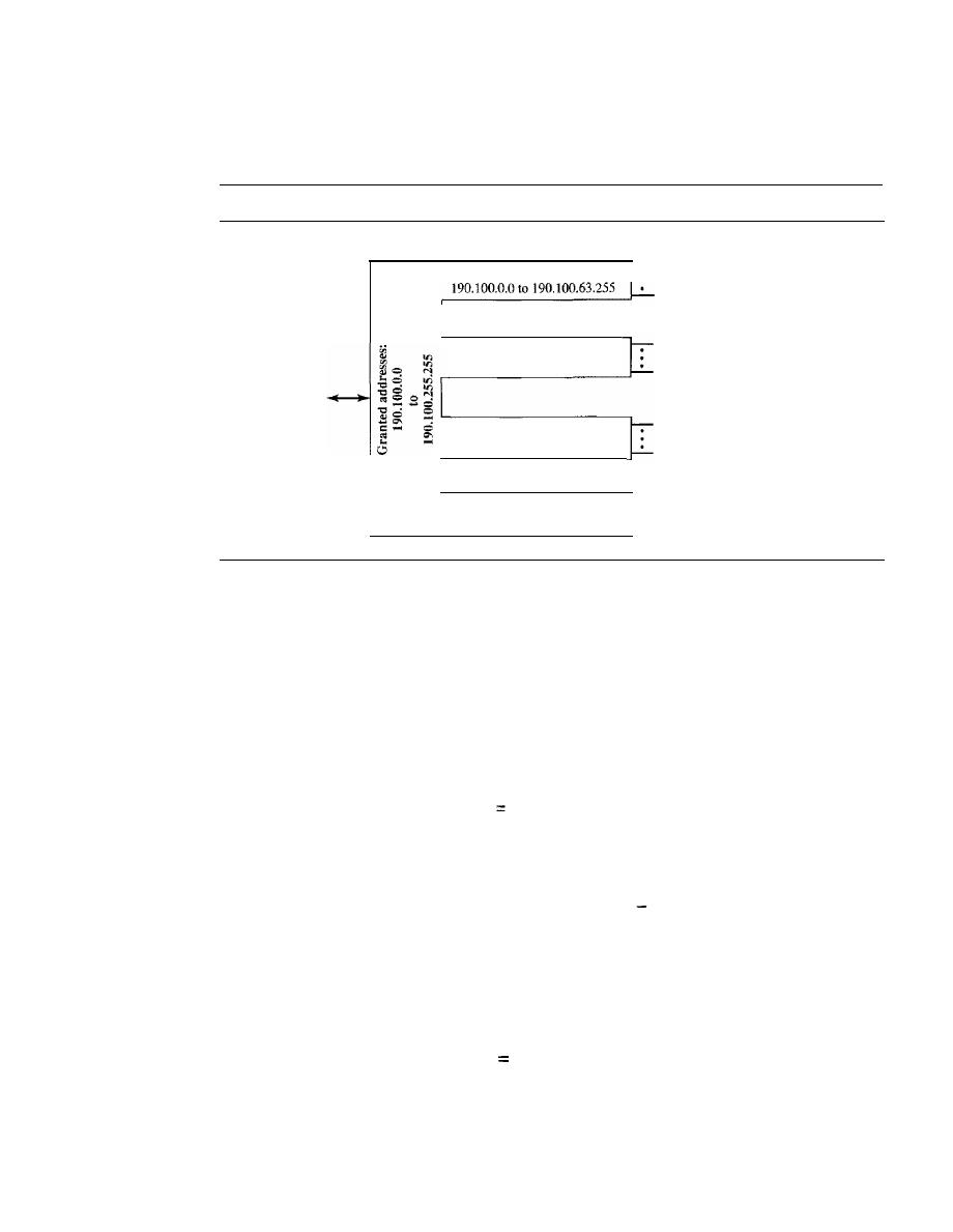
562
CHAPTER 19
NETWORK LAYER: LOGICALADDRESS1NG
Solution
Figure 19.9 shows the situation.
Figure 19.9
An example of address allocation and distribution by an IS?
ISP
Group 1:
Customer 00 1; 190.1 00.0.0/24
Customer 064: 190.100.63.0/24
To and from
the Internet
Group 2:
190.100.64.0 to 190.100.127.255
Group 3:
190.100.128.0 to 190.100.159.255
Available
190.100.160.0 to 190.100.255.255
Customer 00 1: 190.100.64.0/25
Customer 128: 190.100.127.128/25
Customer 001: 190.100.128.0/26
Customer 128: 190.100.159.192/26
1.
Group 1
For this group, each customer needs 256 addresses. This means that 8 (log2256) bits are
needed to define each host. The prefix length is then 32 - 8
=
24. The addresses are
1st Customer:
2nd Customer:
190.100.0.0/24
190.100.1.0/24
190.100.0.255/24
190.100.1.255/24
64th Customer:
190.100.63.0/24
190.100.63.255/24
Total
=
64
X
256
16,384
2. Group2
For this group, each customer needs 128 addresses. This means that 7 (10g2 128) bits are
needed to define each host. The prefix length is then 32
7
=
25. The addresses are
1st Customer:
190.100.64.0/25
2nd Customer:
190.100.64.128/25
190.100.64.127/25
190.100.64.255/25
128th Customer: 190.100.127.128/25
190.100.127.255/25
Total
=
128
X
128
16,384
3. Group3
For this group, each customer needs 64 addresses. This means that 6 (logz 64) bits are needed
to each host. The prefix length is then 32 - 6
=
26. The addresses are

SECTION
19.1
IPv4ADDRESSES
563
1st Customer:
2nd Customer:
190.100.128.0/26
190.100.128.64/26
190.100.128.63/26
190.100.128.127/26
128th Customer: 190.100.159.192/26
190.100.159.255/26
Total
=
128
X
64
=
8192
Number of granted addresses to the ISP: 65,536
Number of allocated addresses by the ISP: 40,960
Number of available addresses: 24,576
Network Address Translation (NAT)
The number of home users and small businesses that want to use the Internet is ever
increasing. In the beginning, a user was connected to the Internet with a dial-up line,
which means that she was connected for a specific period of time. An ISP with a block of
addresses could dynamically assign an address to this user. An address was given to a
user when it was needed. But the situation is different today. Home users and small busi-
nesses can be connected by an ADSL line or cable modem. In addition, many are not
happy with one address; many have created small networks with several hosts and need
an IP address for each host. With the shortage of addresses, this is a serious problem.
A quick solution to this problem is called network address translation
(NAT).
NAT enables a user to have a large set of addresses internally and one address, or a small
set of addresses, externally. The traffic inside can use the large set; the traffic outside, the
small set.
To separate the addresses used inside the home or business and the ones used for
the Internet, the Internet authorities have reserved three sets of addresses as private
addresses, shown in Table 19.3.
Table 19.3
Addresses for private networks
Range
Total
10.0.0.0
to
10.255.255.255
2
24
172.16.0.0
to
172.31.255.255
2
20
192.168.0.0
to
192.168.255.255
2
16
Any organization can use an address out of this set without permission from the
Internet authorities. Everyone knows that these reserved addresses are for private net-
works. They are unique inside the organization, but they are not unique globally. No
router will forward a packet that has one of these addresses as the destination address.
The site must have only one single connection to the global Internet through a router
that runs the NAT software. Figure 19.10 shows a simple implementation of NAT.
As Figure 19.10 shows, the private network uses private addresses. The router that
connects the network to the global address uses one private address and one global
address. The private network is transparent to the rest of the Internet; the rest of the
Internet sees only the NAT router with the address 200.24.5.8.
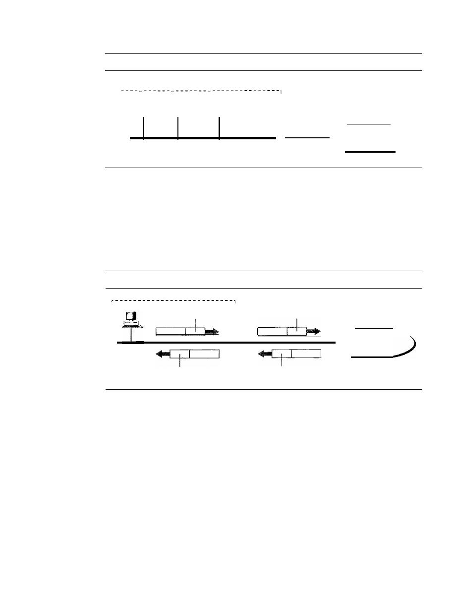
564
CHAPTER
19
NETWORK LAYER: LOGICAL ADDRESSING
Figure 19.10
A NAT implementation
172.18.3.20
...
172.18.3.1
172.18.3.2
Site using private addresses
I
I
I
I
I
I
I
I
NAT
router
172.18.3.30
200.24.5.8
Internet
I
,
_ _ _ _ _ _ _ _ _ _ _ _ _ _ _ _ _ _ _ _ _ _ _ _ _ _ _ _ _ _ _ _ _ _ _ J
Address Translation
All the outgoing packets go through the NAT router, which replaces the source address
in the packet with the global NAT address. All incoming packets also pass through the
NAT router, which replaces the destination address in the packet (the NAT router global
address) with the appropriate private address. Figure 19.11 shows an example of address
translation.
Figure 19.11
Addresses in a NAT
Internet
Source: 200.24.5.8
Destination: 200.24.5.8
Source: 172.18.3.1
Destination: 172.18.3.1
172.18.3.1
I
I
I
I
I
I
I
Translation Table
The reader may have noticed that translating the source addresses for outgoing packets
is straightforward. But how does the NAT router know the destination address for a
packet coming from the Internet? There may be tens or hundreds of private IP addresses,
each belonging to one specific host. The problem is solved if the NAT router has a trans-
lation table.
Using One IP Address
In its simplest fonn, a translation table has only two columns:
the private' address and the external address (destination address of the packet). When
the router translates the source address of the outgoing packet, it also makes note of the
destination address-where the packet is going. When the response comes back from
the destination, the router uses the source address of the packet (as the external address)
to find the private address of the packet. Figure 19.12 shows the idea. Note that the
addresses that are changed (translated) are shown in color.
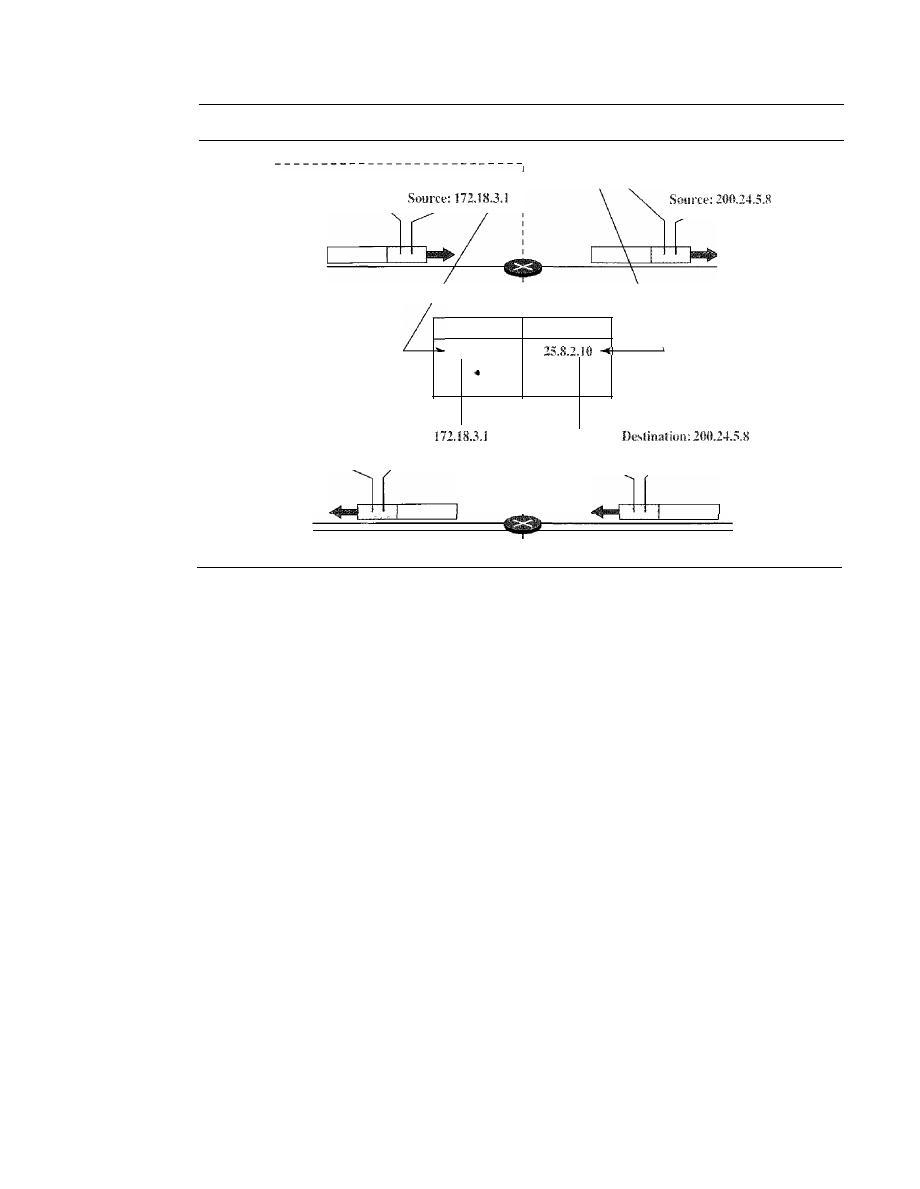
SECTION
19.1
IPv4 ADDRESSES
565
Figure 19.12
NAT address translation
Destination: 25.8.2.10
I
I
I
I
I
I
I
I
I
Destination: 25.8.2.10
Translation table
Private
External
172.18.3.1
.
•
.
I
:
I
Source: 25.8.2.10
I
I
I
I
I
I
Destination:
Source: 25.8.2.10
In this strategy, communication must always be initiated by the private network.
The NAT mechanism described requires that the private network start the communica-
tion. As we will see, NAT is used mostly by ISPs which assign one single address to a
customer. The customer, however, may be a member of a private network that has many
private addresses. In this case, communication with the Internet is always initiated from
the customer site, using a client program such as HTTP, TELNET, or FTP to access the
corresponding server program. For example, when e-mail that originates from a non-
customer site is received by the ISP e-mail server, the e-mail is stored in the mailbox of
the. customer until retrieved. A private network cannot run a server program for clients
outside of its network if it is using NAT technology.
Using a Pool of
IP
Addresses
Since the NAT router has only one global address, only
one private network host can access the same external host. To remove this restriction, the
NAT router uses a pool of global addresses. For example, instead of using only one global
address (200.24.5.8), the NAT router can use four addresses (200.24.5.8, 200.24.5.9,
200.24.5.10, and 200.24.5.11). In this case, four private network hosts can communicate
with the same external host at the same time because each pair of addresses defines a
connection. However, there are still some drawbacks. In this example, no more than four
connections can be made to the same destination. Also, no private-network host can
access two external server programs (e.g., HTTP and
FfP)
at the same time.
Using Both
IP
Addresses and Port Numbers
To allow a many-to-many relationship
between private-network hosts and external server programs, we need more information
in the translation table. For example, suppose two hosts with addresses 172.18.3.1 and
172.18.3.2 inside a private network need to access the HTTP server on external host
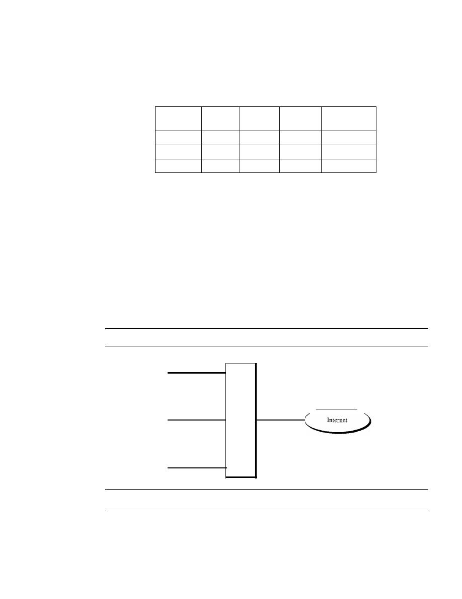
566
CHAPTER
19
NETWORK LAYER: LOGICAL ADDRESSING
25.8.3.2.
If
the translation table has five columns, instead of two, that include the source
and destination port numbers of the transport layer protocol, the ambiguity is eliminated.
We discuss port numbers in Chapter 23. Table 19.4 shows an example of such a table.
Table 19.4
Five-column translation table
Private
Private
External
External
Transport
Address
Port
Address
Port
Protocol
172.18.3.1
1400
25.8.3.2
80
TCP
172.18.3.2
1401
25.8.3.2
80
TCP
..
.
..
.
. ..
.. .
...
Note that when the response from HTTP comes back, the combination of source
address (25.8.3.2) and destination port number (1400) defines the-private network host
to which the response should be directed. Note also that for this translation to work, the
temporary port numbers (1400 and 1401) must be unique.
NAT and ISP
An ISP that serves dial-up customers can use NAT technology to conserve addresses.
For example, suppose an ISP is granted 1000 addresses, but has 100,000 customers.
Each of the customers is assigned a private network address. The ISP translates each of
the 100,000 source addresses in outgoing packets to one of the 1000 global addresses;
it translates the global destination address in incoming packets to the corresponding
private address. Figure 19.13 shows this concept.
Figure 19.13
An ISP and NAT
172.18.3.1
···
172.24.1.1
ISP
site
·
•
•
172.30,100
19.2
IPv6 ADDRESSES
1000
addresses
Despite all short-term solutions, such as classless addressing, Dynamic Host Configu-
ration Protocol (DHCP), discussed in Chapter 21, and NAT, address depletion is still a
long-term problem for the Internet. This and other problems in the IP protocol itself,

SECTION
19.2
IPv6 ADDRESSES
567
such as lack of accommodation for real-time audio and video transmission, and encryp-
tion and authentication of data for some applications, have been the motivation for IPv6.
In this section, we compare the address structure of IPv6 to IPv4. In Chapter 20, we
discuss both protocols.
Structure
An
IPv6 address
consists of 16 bytes (octets);
it
is 128 bits long.
An
IPv6
address is
128
bits long.
Hexadecimal Colon Notation
To make addresses more readable, IPv6 specifies
hexadecimal
colon notation. In this nota-
tion, 128 bits is divided into eight sections, each 2 bytes in length. Two bytes in hexadecimal
notation requires four hexadecimal digits. Therefore, the address consists of 32 hexadecimal
digits, with every four digits separated by a colon, as shown in Figure 19.14.
Figure 19.14
IPv6 address in binary and hexadecimal colon notation
I·
1111110111101100
128 bits
=
16 bytes
=
32 hex digits
1111111111111111
I
FDEC
I:I
0074
I:
I
0000
I:
0000
I:
I
0000
I: I
BOFF
I:
I
0000
I: I
FFFF
I
Abbreviation
Although the IP address, even in hexadecimal format, is very long, many of the digits are
zer9s. In this case, we can abbreviate the address. The leading zeros of a section (four
digits between two colons) can be omitted. Only the leading zeros can be dropped, not
the trailing zeros (see Figure 19.15).
Figure 19.15
Abbreviated IPv6 addresses
Original
FDEC: 0074 : 0000 : 0000 : 0000 : BOFF : 0000 : FFFO
Abbreviated
FDEC: 74 : 0 : 0 : 0 : BOFF : 0 : FFFO

568
CHAPTER
19
NETWORK LAYER: LOGICAL ADDRESSING
Using this form of abbreviation, 0074 can be written as 74, OOOF as F, and 0000 as O.
Note that 3210 cannot be abbreviated. Further abbreviations are possible if there are
consecutive sections consisting of zeros only. We can remove the zeros altogether and
replace them with a double semicolon. Note that this type of abbreviation is allowed
only once per address.
If
there are two runs of zero sections, only one of them can be
abbreviated. Reexpansion of the abbreviated address is very simple: Align the unabbre-
viated portions and insert zeros to get the original expanded address.
Example 19.11
Expand the address 0:15::1:12:1213 to its original.
Solution
We first need to align the left side of the double colon to the left of the original pattern and the
right side of the double colon to the right of the original pattern to find now many Os we need to
replace the double colon.
xxxx:xxxx:xxxx:xxxx:xxxx:xxxx:xxxx:xxxx
0:
15:
l:
12: 1213
This means that the original address is
0000:0015:0000:0000:0000:0001 :0012: 1213
Address Space
IPv6 has a much larger address space; 2
128
addresses are available. The designers of
IPv6 divided the address into several categories. A few leftmost bits, called the type
prefix,
in each address define its category. The type prefix is variable in length, but it is
designed such that no code is identical to the first part of any other code. In this way,
there is no ambiguity; when an address is given, the type prefix can easily be deter-
mined. Table 19.5 shows the prefix for each type of address. The third column shows
the fraction of each type of address relative to the whole address space.
Table 19.5
Type prefixes for 1Pv6 addresses
Type Prefix
Type
Fraction
00000000
Reserved
1/256
00000001
Unassigned
1/256
0000001
ISO network addresses
1/128
0000010
IPX (Novell) network addresses
1/128
0000011
Unassigned
1/128
00001
Unassigned
1/32
0001
Reserved
1/16
001
Reserved
1/8
010
Provider-based unicast addresses
1/8
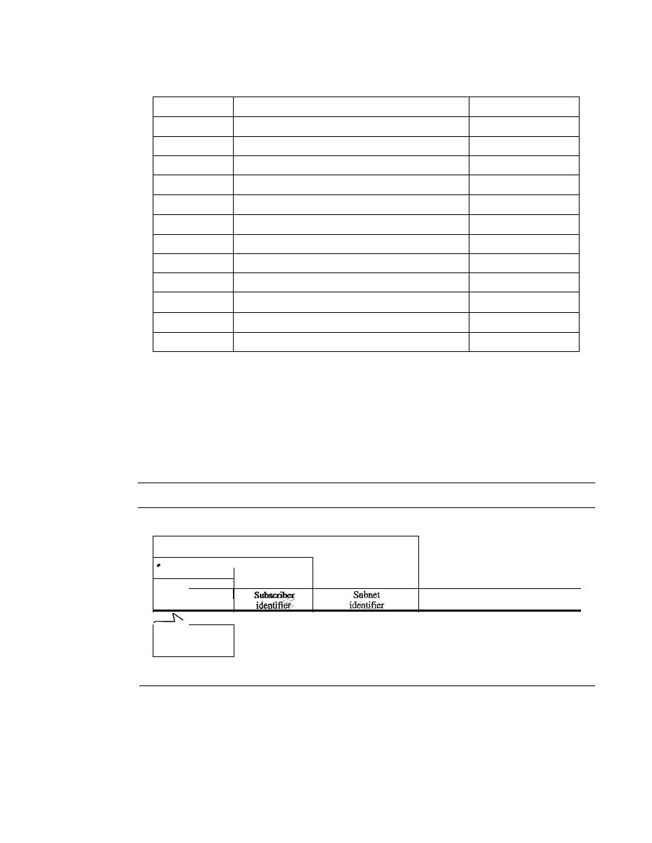
SECTION
19.2
IPv6 ADDRESSES
569
Table 19.5
Type prefixes for IPv6 addresses (continued)
Type Prefix
Type
Fraction
011
Unassigned
1/8
100
Geographic-based unicast addresses
1/8
101
Unassigned
1/8
110
Unassigned
1/8
1110
Unassigned
1116
11110
Unassigned
1132
1111 10
Unassigned
1/64
1111 110
Unassigned
1/128
11111110
a
Unassigned
1/512
1111 111010
Link local addresses
111024
1111 1110 11
Site local addresses
1/1024
11111111
Multicast addresses
1/256
Unicast Addresses
A unicast address defines a single computer. The packet sent to a unicast address must
be delivered to that specific computer. IPv6 defines two types of unicast addresses: geo-
graphically based and provider-based. We discuss the second type here; the first type is
left for future definition. The provider-based address is generally used by a normal host
as a unicast address. The address format is shown in Figure 19.16.
Figure 19.16
Prefixes for provider-based unicast address
Subnet prefix
Subscriber prefix
Provider prefix
151
Provider
Node
I
identifier
identifier
INTERNIC
11000
RIPNIC
01000
APNIC
10100
Registry
Fields for the provider-based address are as follows:
o
Type identifier.
This 3-bit field defines the address as a provider-base.d address.
o
Registry identifier.
This 5-bit field indicates the agency that has registered the
address. Currently three registry centers have been defined. INTERNIC (code
11000) is the center for North America; RIPNIC (code 01000) is the center for
European registration; and APNIC (code 10100) is for Asian and Pacific countries.
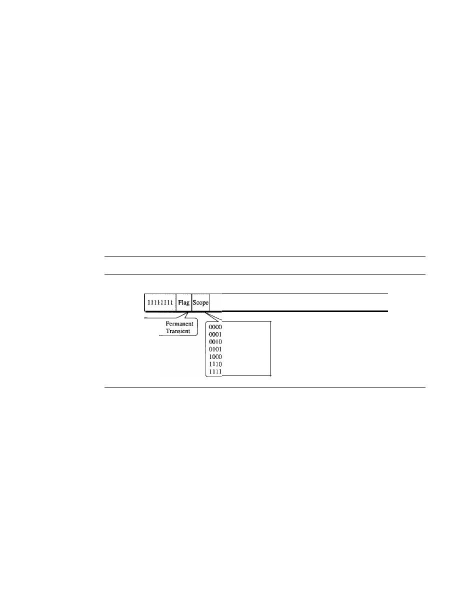
570
CHAPTER
19
NETWORK LAYER: LOGICAL ADDRESSING
o
Provider identifier.
This variable-length field identifies the provider for Internet
access (such as an ISP). A 16-bit length is recommended for this field.
o
Subscriber identifier.
When an organization subscribes to the Internet through a
provider, it is assigned a subscriber identification. A 24-bit length is recommended
for this field.
o
Subnet identifier.
Each subscriber can have many different subnetworks, and each
subnetwork can have an identifier. The subnet identifier defines a specific subnetwork
under the territory of the subscriber. A 32-bit length is recommended for this field.
o
Node identifier.
The last field defines the identity of the node connected to a subnet.
A length of 48 bits is recommended for this field to make it compatible with the
48-bit link (physical) address used by Ethernet. In the future, this link address will
probably be the same as the node physical address.
Multicast Addresses
Multicast addresses are used to define a group of hosts instead of just one. A packet sent
to a
multicast address
must be delivered to each member of the group. Figure 19.17
shows the format of a multicast address.
Figure 19.17
Multicast address in IPv6
8 bits
0000
0001
4
4
Reserved
Node local
Link local
Site local
Organizational
Global
Reserved
112 bits
Group ID
The second field is a flag that defines the group address as either permanent or
transient. A permanent group address is defined by the Internet authorities and can be
accessed at all times. A transient group address, on the other hand, is used only tempo-
rarily. Systems engaged in a teleconference, for example, can use a transient group
address. The third field defines the scope of the group address. Many different scopes
have been defined, as shown in Figure 19.17.
Allycast Addresses
IPv6 also defines anycast addresses. An
anycast address,
like a multicast address, also
defines a group of nodes. However, a packet destined for an anycast address is delivered
to only one ofthe members of the anycast group, the nearest one (the one with the shortest
route). Although the definition of an anycast address is still debatable, one possible use
is to assign an anycast address to all routers of an ISP that covers a large logical area in
the Internet. The routers outside the ISP deliver a packet destined for the ISP to the
nearest ISP router. No block is assigned for anycast addresses.
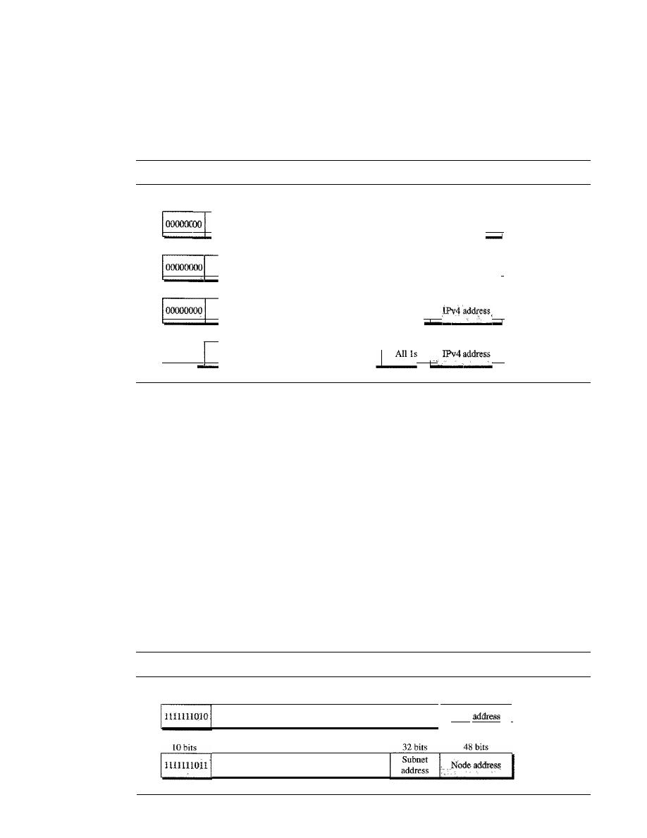
SECTION
19.2
IPv6 ADDRESSES
571
Reserved Addresses
Another category in the address space is the
reserved address.
These addresses start
with eight Os (type prefix is 00000000). A few subcategories are defined in this category,
as shown in Figure 19.18.
Figure 19.18
Reserved addresses in IPv6
8
bits
120 bits
A_ll_os
1
a. Unspecified
8
bits
120 bits
°_0_00_0_00_0_00_0_00_0_00_0_",_",_"'_",_,,,_,°_00_0_00_0_00_0_1
1
b. Loopback
8
bits
88
bits
32 bits
32 bits
16 bits
72
bits
A_I_1
o_s
I
1
c.
Compatible
8
bits
l_o_oooooo
__
o
A_
ll_O_
S
__
I
_I
d. Mapped
An
unspecified address
is used when a host does not know its own address and
sends an inquiry to find its address. A
loopback address
is used by a host to test itself
without going into the network. A
compatible address
is used during the transition
from IPv4 to IPv6 (see Chapter 20).
It
is used when a computer using IPv6 wants to
send a message to another computer using IPv6, but the message needs to pass through
a part of the network that still operates in IPv4. A
mapped address
is also used during
transition. However, it is used when a computer that has migrated to IPv6 wants to send
a packet to a computer still using IPv4.
Local Addresses
.
These addresses are used when an organization wants to use IPv6 protocol without being
connected to the global Internet. In other words, they provide addressing for private net-
works. Nobody outside the organization can send a message to the nodes using these
addresses. Two types of addresses are defined for this purpose, as shown in Figure 19.19.
Figure 19.19
Local addresses in IPv6
10 bits
70 bits
All
Os
48 bits
Node
I
a. Link local
38 bits
All Os
b. Site local

572
CHAPTER
19
NETWORK LAYER: LOGICAL ADDRESSING
A link local address is used in an isolated subnet; a site local address is used in
an isolated site with several subnets.
19.3
RECOMMENDED READING
For more details about subjects discussed in this chapter, we recommend the following
books and sites. The items in brackets [...] refer to the reference list at the end of
the text.
Books
IPv4 addresses are discussed in Chapters 4 and 5 of [For06], Chapter 3 of [Ste94], Sec-
tion 4.1 of [PD03], Chapter 18 of [Sta04], and Section 5.6 of
IPv6 addresses
are discussed in Section 27.1 of [For06] and Chapter 8 of [Los04]. A good discussion of
NAT can be found in [DutOl].
Sites
o
www.ietf.org/rfc.html
Information about RFCs
RFCs
A discussion of IPv4 addresses can be found in most of the RFCs related to the IPv4
protocol:
760,781,791,815,1025,1063,1071,1141,1190, 1191, 1624,2113
A discussion of 1Pv6 addresses can be found in most of the RFCs related to IPv6 protocol:
1365,1550,1678,1680,1682,1683,1686,1688,1726, 1752, 1826, 1883, 1884,1886,1887,
1955,2080,2373,2452,2463,2465,2466,2472,2492,2545,2590
A discussion of NAT can be found in
1361,2663,2694
19.4
KEY TERMS
address aggregation
address space
anycast address
binary notation
class A address
class B address
class C address
class D address
class E address
classful addressing
classless addressing
classless interdomain routing (CIDR)

compatible address
dotted-decimal notation
default mask
hexadecimal colon notation
hostid
IP address
IPv4 address
IPv6 address
link local address
mapped address
mask
multicast address
netid
network address
SECTION
19.5
SUMMARY
573
network address translation
(NAT)
prefix
reserved address
site local address
subnet
subnet mask
subnetting
suffix
supernet
supernet mask
supernetting
unicast address
unspecified address
19.5
SUMMARY
o
At the network layer, a global identification system that uniquely identifies every
host and router is necessary for delivery of a packet from host to host.
o
An IPv4 address is 32 bits long and uniquely and universally defines a host or
router on the Internet.
o
In classful addressing, the portion of the IP address that identifies the network is
called the netid.
o
In classful addressing, the portion of the IP address that identifies the host or router
on the network is called the hostid.
o
An IP address defines a device's connection to a network.
o
There are five classes in IPv4 addresses. Classes A, B, and C differ in the number
of hosts allowed per network. Class D is for multicasting and Class E is reserved.
o
The class of an address is easily determined by examination of the first byte.
o
Addresses in classes A, B, or C are mostly used for unicast communication.
o
Addresses in class D are used for multicast communication.
o
Subnetting divides one large network into several smaller ones, adding an interme-
diate level of hierarchy in IP addressing.
o
Supernetting combines several networks into one large one.
o
In classless addressing, we can divide the address space into variable-length blocks.
o
There are three restrictions in classless addressing:
a. The number of addresses needs to be a power of 2.
b. The mask needs to be included in the address to define the block.
c. The starting address must be divisible by the number of addresses in the block.
o
The mask in classless addressing is expressed as the prefix length
(In)
in CIDR notation.

574
CHAPTER
19
NETWORK LAYER: LOGICAL ADDRESSING
o
To find the first address in a block, we set the rightmost 32 -
n
bits to O.
o
To find the number of addresses in the block, we calculate
2
32
-
n
,
where
n
is the
prefix length.
o
To find the last address in the block, we set the rightmost 32 - n bits to O.
o
Subnetting increases the value of n.
o
The global authority for address allocation is ICANN. ICANN normally grants
large blocks of addresses to ISPs, which in tum grant small subblocks to individual
customers.
o
IPv6 addresses use hexadecimal colon notation with abbreviation methods available.
o
There are three types of addresses in IPv6: unicast, anycast, and multicast.
o
In an IPv6 address, the variable type prefix field defines the address type or purpose.
19.6
PRACTICE SET
Review Questions
1.
What is the number of bits in an IPv4 address? What is the number of bits in an
IPv6 address?
2. What is dotted decimal notation in IPv4 addressing? What is the number of bytes
in an IPv4 address represented in dotted decimal notation? What is hexadecimal
notation in IPv6 addressing? What is the number of digits in an IPv6 address repre-
sented in hexadecimal notation?
3. What are the differences between classful addressing and classless addressing in IPv4?
4. List the classes in classful addressing and define the application of each class (unicast,
multicast, broadcast, or reserve).
5. Explain why most of the addresses in class A are wasted. Explain why a medium-size
or large-size corporation does not want a block of class C addresses.
6. What is a mask in IPv4 addressing? What is a default mask in IPv4 addressing?
7. What is the network address in a block of addresses? How can we find the network
address if one of the addresses in a block is given?
8. Briefly define subnetting and supemetting. How do the subnet mask and supemet
mask differ from a default mask in classful addressing?
9. How can we distinguish a multicast address in IPv4 addressing? How can we do so
in IPv6 addressing?
10. What is NAT? How can NAT help in address depletion?
Exercises
II.
What is the address space in each of the following systems?
a. A system with 8-bit addresses
b. A system with 16-bit addresses
c. A system with 64-bit addresses

SECTION
19.6
PRACTICE SET
575
12. An address space has a total of 1024 addresses. How many bits are needed to rep-
resent an address?
13. An address space uses the three symbols 0, 1, and 2 to represent addresses.
If
each address is made of 10 symbols, how many addresses are available in this
system?
14. Change the following IP addresses from dotted-decimal notation to binary notation.
a.
114.34.2.8
b.
129.14.6.8
c.
208.34.54.12
d. 238.34.2.1
15. Change the following IP addresses from binary notation to dotted-decimal notation.
a.
01111111 11110000 01100111 01111101
b.
10101111 11000000 11111000 00011101
c. 11011111 10110000 00011111 01011101
d.
11101111 11110111 11000111 00011101
16. Find the class of the following IP addresses.
a.
208.34.54.12
b.
238.34.2.1
c. 114.34.2.8
d.
129.14.6.8
17. Find the class of the following IP addresses.
a.
11110111 11110011 10000111 11011101
b.
10101111 11000000 11110000 00011101
c. 11011111 10110000 00011111 01011101
d. 11101111 11110111 11000111 00011101
18. Find the netid and the hostid of the following IP addresses.
• a. 114.34.2.8
b. 132.56.8.6
c. 208.34.54.12
19. In a block of addresses, we know the IP address of one host is 25.34.12.56/16.
What are the first address (network address) and the last address (limited broadcast
address) in this block?
20. In a block of addresses, we know the IP address of one host is 182.44.82.16/26.
What are the first address (network address) and the last address in this block?
21.
An
organization is granted the block 16.0.0.0/8. The administrator wants to create
500 fixed-length subnets.
a. Find the subnet mask.
b. Find the number of addresses in each subnet.
c. Find the first and last addresses in subnet 1.
d. Find the first and last addresses in subnet 500.

576
CHAPTER
19
NETWORK LAYER: LOGICAL ADDRESSING
22. An organization is granted the block 130.56.0.0/16. The administrator wants to
create 1024 subnets.
a. Find the subnet mask.
b. Find the number of addresses in each subnet.
c. Find the first and last addresses in subnet 1.
d. Find the first and last addresses in subnet 1024.
23. An organization is granted the block 211.17.180.0/24. The administrator wants to
create 32 subnets.
a. Find the subnet mask.
b. Find the number of addresses in each subnet.
c. Find the first and last addresses in subnet 1.
d. Find the first and last addresses in subnet 32.
24. Write the following masks in slash notation
(In).
a. 255.255.255.0
b. 255.0.0.0
c. 255.255.224.0
d. 255.255.240.0
25. Find the range of addresses in the following blocks.
a. 123.56.77.32/29
b. 200.17.21.128/27
c. 17.34.16.0/23
d. 180.34.64.64/30
26. An ISP is granted a block of addresses starting with 150.80.0.0/16. The ISP wants
to distribute these blocks to 2600 customers as follows.
a. The first group has 200 medium-size businesses; each needs 128 addresses.
b. The second group has 400 small businesses; each needs 16 addresses.
c. The third group has 2000 households; each needs 4 addresses.
Design the subblocks and give the slash notation for each subblock. Find out how
many addresses are still available after these allocations.
27. An ISP is granted a block of addresses starting with 120.60.4.0/22. The ISP
wants to distribute these blocks to 100 organizations with each organization
receiving just eight addresses. Design the subblocks and give the slash notation
for each subblock. Find out how many addresses are still available after these
allocations.
28. An ISP has a block of 1024 addresses.
It
needs to divide the addresses among
1024 customers. Does it need subnetting? Explain your answer.
29. Show the shortest form of the following addresses.
a. 2340: lABC: 119A:AOOO:0000:0000:0000:0000
b. OOOO:OOAA:OOOO:OOOO:OOOO:OOOO: 119A:A231
c. 2340:0000:0000:0000:0000: 119A:AOO1:0000
d. 0000:0000:0000:2340:0000:0000:0000:0000

SECTION
19.6
PRACTICE SET
577
30. Show the original (unabbreviated) form of the following addresses.
a. 0::0
b.O:AA::O
c. 0: 1234::3
d.
123::1:2
What is the type of each of the following addresses?
a.
FE80::12
b.
FECO: :24A2
c. FF02::0
d.
0::01
32. What is the type of each of the following addresses?
a.
0::0
b. 0: :FFFF:O:O
c. 582F:1234::2222
d. 4821::14:22
e. 54EF::A234:2
33. Show the provider prefix (in hexadecimal colon notation) of an address assigned
to a subscriber if it is registered in the United States with ABC1 as the provider
identification.
34. Show in hexadecimal colon notation the IPv6 address
a. Compatible to the IPv4 address 129.6.12.34
b. Mapped to the IPv4 address 129.6.12.34
35. Show in hexadecimal colon notation
a. The link local address in which the node identifier is 0:: 123/48
b. The site local address in which the node identifier is 0:: 123/48
36. Show in hexadecimal colon notation the permanent multicast address used in a link
local scope.
37.• A host has the address 581E: 1456:2314:ABCD:: 1211. If the node identification is
48 bits, find the address of the subnet to which the host is attached.
38. A site with 200 subnets has the class B address of 132.45.0.0. The site recently
migrated to IPv6 with the subscriber prefix 581E:1456:2314::ABCD/80. Design
the subnets and define the subnet addresses, using a subnet identifier of 32 bits.
Research Activities
39. Find the block of addresses assigned to your organization or institution.
40. If you are using an ISP to connect from your home to the Internet, find the name of
the ISP and the block of addresses assigned to it.
41. Some people argue that we can consider the whole address space as one single
block in which each range of addresses is a subblock to this single block. Elaborate
on this idea. What happens to subnetting if we accept this concept?
42. Is your school or organization using a classful address?
If
so, find out the class of
the address.


CHAPTER 20
Network Layer:
Internet Protocol
In the Internet model, the main network protocol is the Internet Protocol (IP). In this
chapter, we first discuss internetworking and issues related to the network layer protocol
in general.
We then discuss the current version of the Internet Protocol, version 4, or IPv4.
This leads us to the next generation of this protocol, or IPv6, which may become the
dominant protocol in the near future.
Finally, we discuss the transition strategies from IPv4 to IPv6. Some readers may
note the absence of IPv5. IPv5 is an experimental protocol, based mostly on the OSI
model that never materialized.
20.1
INTERNETWORKING
The physical and data link layers of a network operate locally. These two layers are
jointly responsible for data delivery on the network from one node to the next, as shown
in Figure 20.1.
This internetwork is made of five networks: four LANs and one WAN.
If
host A
needs to send a data packet to host D, the packet needs to go first from A to Rl (a switch
or router), then from Rl to R3, and finally from R3 to host D. We say that the data packet
passes through three links. In each link, two physical and two data link layers are involved.
However, there is a big problem here. When data arrive at interface
fl
of Rl, how
does RI know that interface
f3
is the outgoing interface? There is no provision in the
data link (or physical) layer to help Rl make the right decision. The frame does not
carry any routing information either. The frame contains the MAC address of A as the
source and the MAC address of Rl as the destination. For a LAN or a WAN, delivery
means carrying the frame through one link, and not beyond.
Need for Network Layer
To solve the problem of delivery through several links, the network layer (or the inter-
network layer, as it is sometimes called) was designed. The network layer is responsible
for host-to-host delivery and for routing the packets through the routers or switches.
Figure 20.2 shows the same internetwork with a network layer added.
579
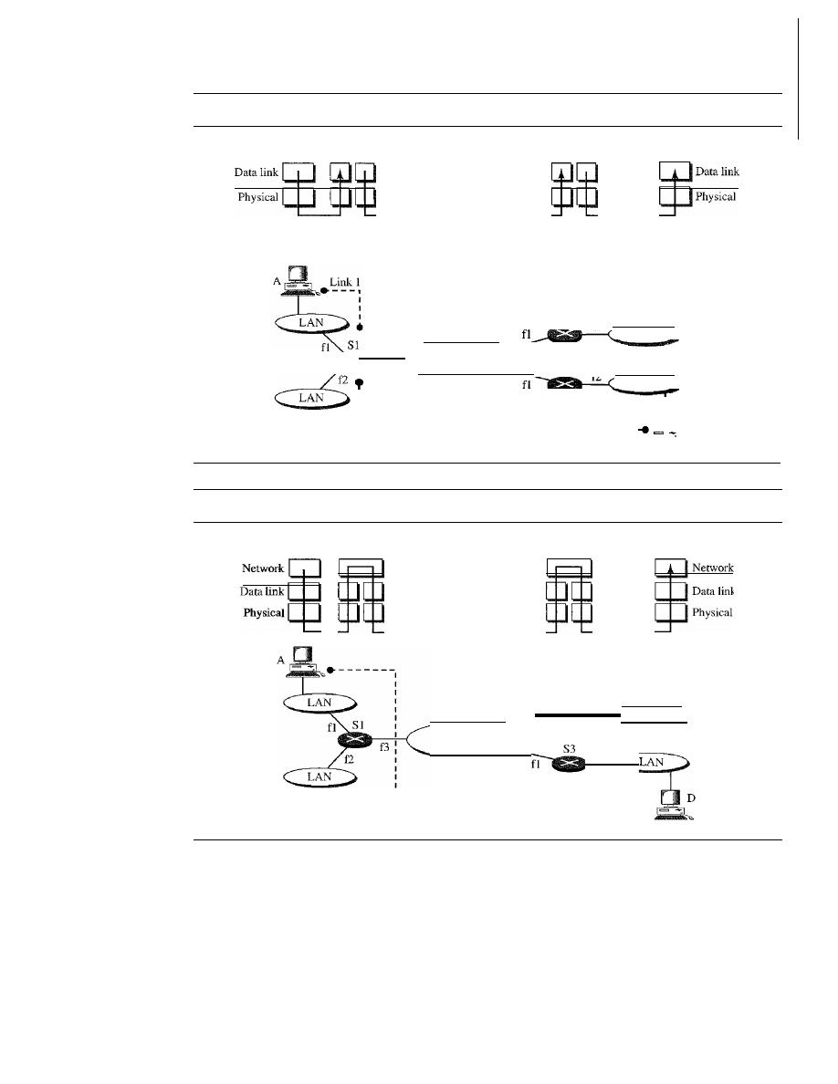
580
CHAPTER
20
NETWORK LAYER: INTERNET PROTOCOL
Figure 20.1
Links between two hosts
A
51
53
0
Physical
Physical
------------
Hop-to-hop
Hop-to-hop
Hop-to-hop
delivery
delivery
delivery
LAN
LAN
Link 3
0
.
-------
53
52
f2
WAN
f3
f2
I
I
I
I
Link 2
L
•
Figure 20.2
Network layer in an internetwork
A
Physical
51
53
D
Data link
_ _ _ _ _
_ _
Physical
-----------------------------.
Host-to-host path
LAN
f2
f2
52
fl
WAN
Figure 20.3 shows the general idea of the functionality of the network layer at a
source, at a router, and at the destination. The network layer at the source is responsible
for creating a packet from the data coming from another protocol (such as a transport
layer protocol or a routing protocol). The header of the packet contains, among other
information, the logical addresses of the source and destination. The network layer is
responsible for checking its routing table to find the routing information (such as the
outgoing interface of the packet or the physical address of the next node).
If
the packet
is too large, the packet is fragmented (fragmentation is discussed later in this chapter).
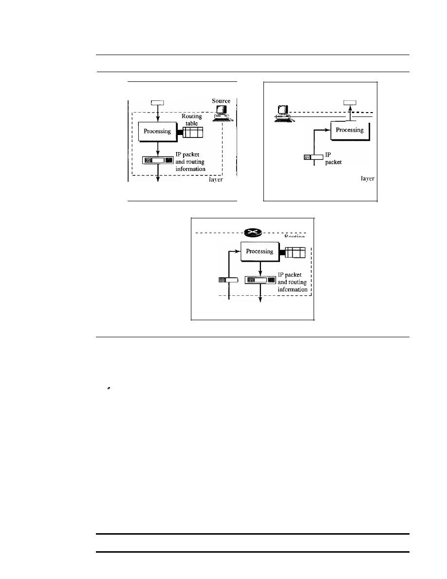
SECTION 20.1
1NTERNETWORKING
S8t
Figure 20.3
Network layer at the source, router, and destination
____________ ...1
Network
Data to
another protocol
Destination
Network
Data from
another protocol
To data
link layer
From data
link layer
a. Network layer at source
b. Network layer at destination
Router
Routing
table
lP
packet
Network layer
From data
To data
.
link layer
link layer
c. Network layer at a router
The network layer at the switch or router is responsible for routing the packet.
When a packet arrives, the router or switch consults its routing table and finds the inter-
face from which the packet must be sent. The packet, after some changes in the header,
with the routing infonnation is passed to the data link layer again.
The network layer at the destination is responsible for address verification; it makes
sure that the destination address on the packet is the same as the address of the host. If
the packet is a fragment, the network layer waits until all fragments have arrived, and
then reassembles them and delivers the reassembled packet to the transport layer.
Internet
as a Datagram Network
The Internet, at the network layer, is a packet-switched network. We discussed switching
in Chapter 8. We said that, in general, switching can be divided into three broad catego-
ries: circuit switching, packet switching, and message switching. Packet switching uses
either the virtual circuit approach or the datagram approach.
The Internet has chosen the datagram approach to switching in the network layer.
It
uses the universal addresses defined in the network layer to route packets from the
source to the destination.
Switching at the network layer
in
the Internet uses the datagram approach to packet switching.
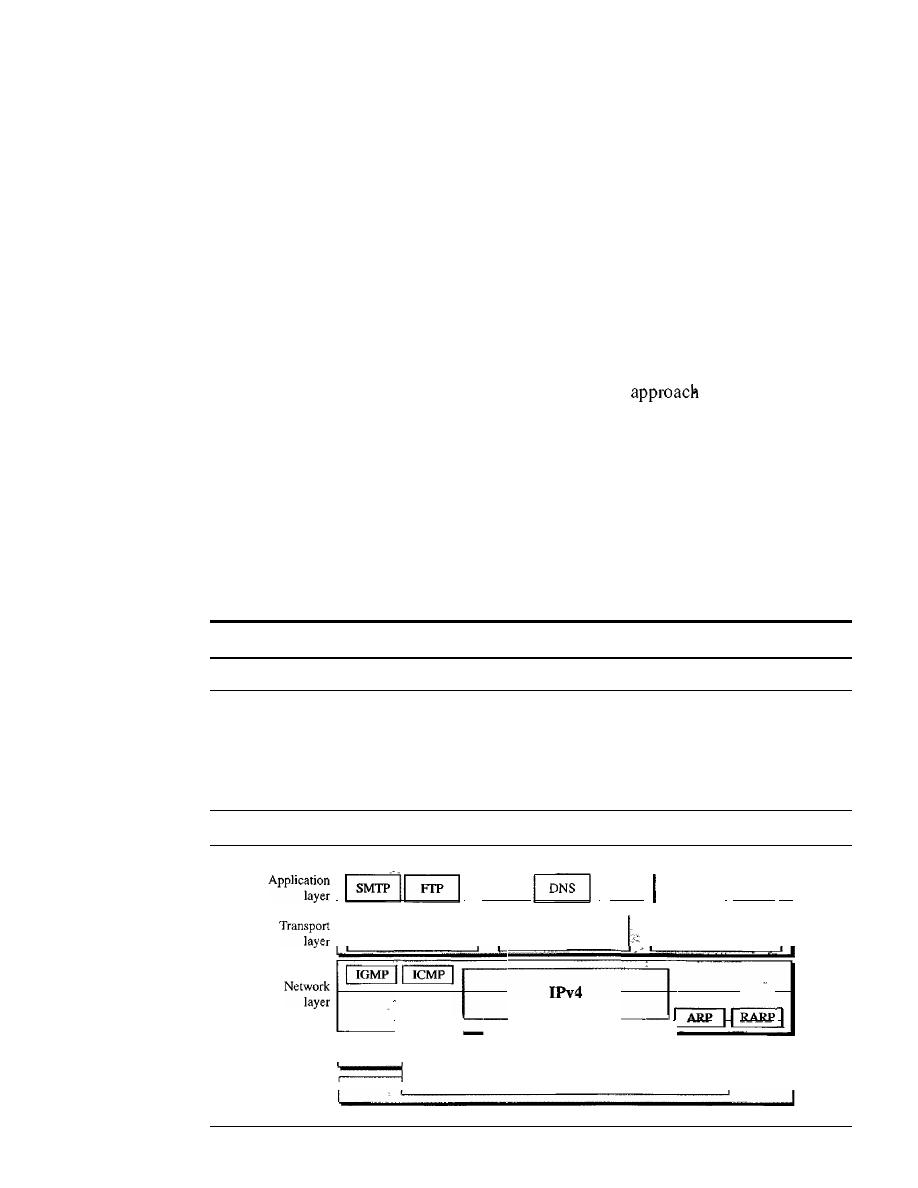
582
CHAPTER 20
NETWORK LAYER: INTERNET PROTOCOL
Internet as a Connectionless Network
Delivery of a packet can be accomplished by using either a connection-oriented or a
connectionless network service. In a
connection-oriented service, the source first
makes a connection with the destination before sending a packet. When the connection
is established, a sequence of packets from the same source to the same destination can
be sent one after another.
In
this case, there is a relationship between packets. They are
sent on the same path in sequential order. A packet is logically connected to the packet
traveling before it and to the packet traveling after it. When all packets of a message
have been delivered, the connection is terminated.
In a connection-oriented protocol, the decision about the route of a sequence of
packets with the same source and destination addresses can be made only once, when
the connection is established. Switches do not recalculate the route for each individual
packet. This type of service is used in a virtual-circuit
to packet switching
such as in Frame Relay and ATM.
In
conneetionless service, the network layer protocol treats each packet indepen-
dently, with each packet having no relationship to any other packet. The packets in a
message mayor may not travel the same path to their destination. This type of service
is used in the datagram approach to packet switching. The Internet has chosen this type
of service at the network layer.
The reason for this decision is that the Internet is made of so many heterogeneous
networks that it is almost impossible to create a connection from the source to the
destination without knowing the nature of the networks in advance.
Communication at the network layer in the Internet is connectionless.
20.2
IPv4
The
Internet Protocol version 4 (IPv4) is the delivery mechanism used by the TCP/IP
protocols. Figure 20.4 shows the position of IPv4 in the suite.
Figure 20.4
Position ofIPv4 in TCPIIP protocol suite
I
I
TFTPI
I
SNMP
••• I
BOOTP II
11
SCTP
I I
TCP
I
UDP
II
IGMP
ICMP
I
ARP
II
Data link
I
I
layer
Underlying LAN or WAN
Physical
I
technology
I
layer
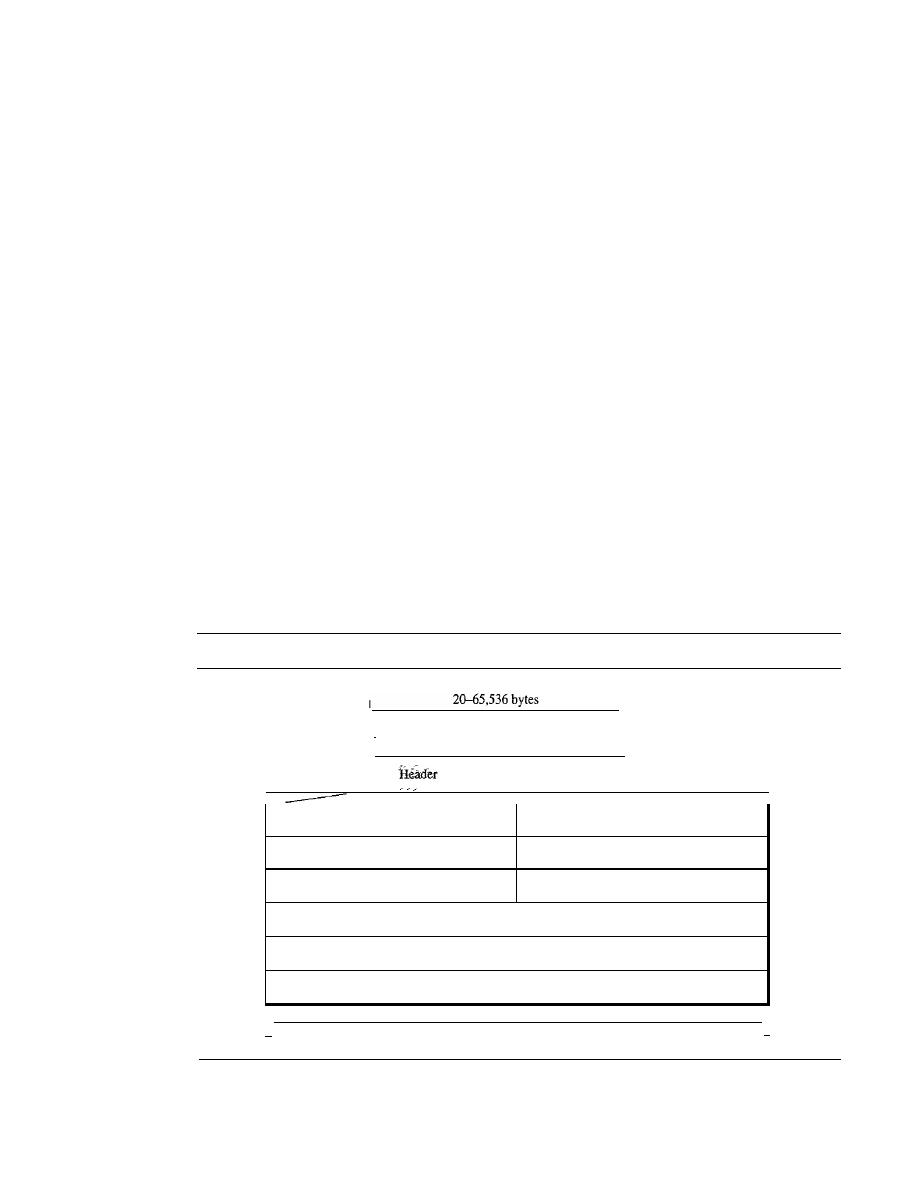
SECTION 20.2
IPv4
583
IPv4 is an unreliable and connectionless datagram protocol-a best-effort delivery
service. The term
best-effort
means that IPv4 provides no error control or flow control
(except for error detection on the header). IPv4 assumes the unreliability of the under-
lying layers and does its best to get a transmission through to its destination, but with
no guarantees.
If
reliability is important, IPv4 must be paired with a reliable protocol such as TCP.
An example of a more commonly understood best-effort delivery service is the post
office. The post office does its best to deliver the mail but does not always succeed.
If
an unregistered letter is lost, it is up to the sender or would-be recipient to discover the
loss and rectify the problem. The post office itself does not keep track of every letter
and cannot notify a sender of loss or damage.
IPv4 is also a connectionless protocol for a packet-switching network that uses the
datagram approach (see Chapter 8). This means that each datagram is handled indepen-
dently, and each datagram can follow a different route to the destination. This implies
that datagrams sent by the same source to the same destination could arrive out of
order. Also, some could be lost or corrupted during transmission. Again, IPv4 relies on
a higher-level protocol to take care of all these problems.
Datagram
Packets in the IPv4 layer are called datagrams. Figure 20.5 shows the IPv4 datagram
format.
Figure 20.5
IPv4 datagramfannat
: 20-60 bytes
"I
I
Data
I
VER
I
HLEN
I
Service
Total length
4 bits
4 bits
8 bits
16 bits
Identification
Flags
I
Fragmentation offset
16 bits
3 bits
13 bits
Time to live
I
Protocol
Header checksum
8 bits
8 bits
16 bits
Source IP address
Destination IP address
Option
I·
32 bits
-I
A datagram is a variable-length packet consisting of two parts: header and data.
The header is 20 to 60 bytes in length and contains information essential to routing and
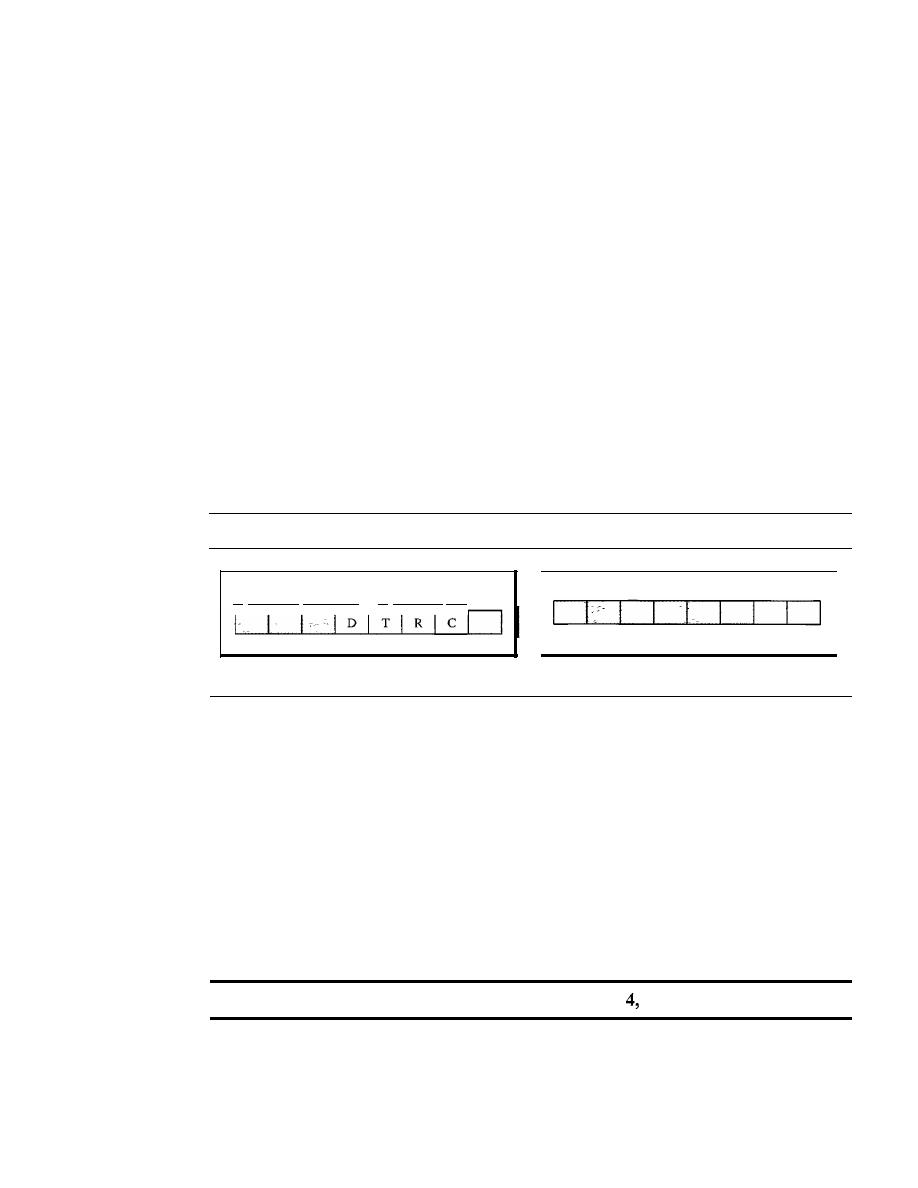
584
CHAPTER 20
NETWORK LAYER: INTERNET PROTOCOL
delivery.
It
is customary in
TCP/IP to show the header in 4-byte sections. A brief
description of each field is in order.
o
Version (VER). This 4-bit field defines the version of the IPv4 protocol. Currently
the version is 4. However, version 6 (or IPng) may totally replace version 4 in the
future. This field tells the IPv4 software running in the processing machine that the
datagram has the format of version 4. All fields must be interpreted as specified
in the fourth version of the protocol.
If
the machine is using some other version of
IPv4, the datagram is discarded rather than interpreted incorrectly.
o
Header length (HLEN). This 4-bit field defines the total length of the datagram
header in 4-byte words. This field is needed because the length of the header
is variable (between 20 and 60 bytes). When there are no options, the header length
is 20 bytes, and the value of this field is 5 (5 x 4
=
20). When the option field is
at its maximum size, the value of this field is 15 (15 x 4
=
60).
o
Services. IETF has changed the interpretation and name of this 8-bit field. This
field, previously called
service type, is now called differentiated services. We show
both interpretations in Figure 20.6.
Figure 20.6
Service type or differentiated services
D: Minimize delay
R: Maximize reliability
T: Maximize throughput
C: Minimize cost
Precedence
TOS bits
Service type
Codepoint
Differentiated services
1.
Service Type
In this interpretation, the first 3 bits are called precedence bits. The next 4 bits are
called
type of service (TOS) bits, and the last bit is not used.
a.
Precedence is a 3-bit subfield ranging from 0 (000 in binary) to 7 (111 in binary).
The precedence defines the priority of the datagram in issues such as congestion.
If
a router is congested and needs to discard some datagrams, those datagrams
with lowest precedence are discarded first. Some datagrams in the Internet are
more important than others. For example, a datagram used for network manage-
ment is much more urgent and important than a datagram containing optional
information for a group.
The precedence subfield was part of version
but never used.
b.
TOS bits is a 4-bit subfield with each bit having a special meaning. Although a
bit can be either 0 or 1, one and only one of the bits can have the value of 1 in
each datagram. The bit patterns and their interpretations are given in Table 20.1.
With only 1 bit set at a time, we can have five different types of services.
SECTION 20.2
IPv4
585
Table 20.1
Types of service
TOS Bits
Description
0000
Normal (default)
0001
Minimize cost
0010
Maximize reliability
0100
Maximize throughput
1000
Minimize delay
Application programs can request a specific type of service. The defaults for some
applications are shown in Table 20.2.
Table 20.2
Default types of service
Protocol
TOS Bits
Description
ICMP
0000
Normal
BOOTP
0000
Normal
NNTP
0001
Minimize cost
IGP
0010
Maximize reliability
SNMP
0010
Maximize reliability
TELNET
1000
Minimize delay
FTP (data)
0100
Maximize throughput
FTP (control)
1000
Minimize delay
TFTP
1000
Minimize delay
SMTP (command)
1000
Minimize delay
SMTP (data)
0100
Maximize throughput
DNS (UDP query)
1000
Minimize delay
DNS (TCP query)
0000
Normal
DNS (zone)
0100
Maximize throughput
It
is clear from Table 20.2 that interactive activities, activities requiring immediate
attention, and activities requiring immediate response need minimum delay. Those
activities that send bulk data require maximum throughput. Management activities
need maximum reliability. Background activities need minimum cost.
2. Differentiated Services
In
this interpretation, the first 6 bits make up the codepoint subfield, and the last 2 bits
are not used. The codepoint subfield can be used in two different ways.
a. When the 3 rightmost bits are Os, the 3 leftmost bits are interpreted the same as the
precedence bits in the service type interpretation. In other words, it is compatible
with the old interpretation.

586
CHAPTER 20
NE1WORK LAYER: INTERNET PROTOCOL
b.
When the 3 rightmost bits are not all Os, the 6 bits define 64 services based on the
priority assignment by the Internet or local authorities according to Table 20.3. The
first category contains 32 service types; the second and the third each contain 16.
The first category (numbers 0, 2,4, ... ,62) is assigned by the Internet authorities
(IETF). The second category (3, 7, 11, 15,
, 63) can be used by local authorities
(organizations). The third category (1, 5, 9,
,61) is temporary and can be used
for experimental purposes. Note that the numbers are not contiguous.
If
they were,
the first category would range from 0 to 31, the second from 32 to 47, and the third
from 48 to 63. This would be incompatible with the TOS interpretation because
XXXOOO (which includes 0, 8, 16, 24, 32, 40, 48, and 56) would fall into all
three categories. Instead, in this assignment method all these services belong to
category
1.
Note that these assignments have not yet been finalized.
Table 20.3
Values for codepoints
Category
Codepoint
Assigning Authority
1
XXXXXO
Internet
2
XXXXll
Local
3
XXXXOI
Temporary or experimental
o
Total length. This
a In-bit field that defines the total length (header plus data)
of the IPv4 datagram in bytes. To find the length of the data coming from the upper
layer, subtract the header length from the total length. The header length can be
found by multiplying the value in the HLEN field by 4.
Length of data
=
total length - header length
Since the field length is 16 bits, the total length of the IPv4 datagram is limited to
65,535 (2
16
-
1) bytes, of which 20 to 60 bytes are the header and the rest is data
from the upper layer.
The total length field defines the total length of the datagram including the header.
Though a size of 65,535 bytes might seem large, the size of the IPv4 datagram
may increase in the near future as the underlying technologies allow even more
throughput (greater bandwidth).
When we discuss fragmentation in the next section, we will see that some phys-
ical networks are not able to encapsulate a datagram of 65,535 bytes in their frames.
The datagram must be fragmented to be able to pass through those networks.
One may ask why we need this field anyway. When a machine (router or host)
receives a frame, it drops the header and the trailer, leaving the datagram. Why
include an extra field that is not needed? The answer is that in many cases we
really do not need the value in this field. However, there are occasions in which the

SECTION 20.2
IPv4
587
datagram is not the only thing encapsulated in a frame; it may be that padding has
been added. For example, the Ethernet protocol has a minimum and maximum
restriction on the size of data that can be encapsulated in a frame (46 to 1500 bytes).
If
the size of an IPv4 datagram is less than 46 bytes, some padding will be added to
meet this requirement. In this case, when a machine decapsulates the datagram, it
needs to check the total length field to determine how much is really data and how
much is padding (see Figure 20.7).
Figure 20.7
Encapsulation of a small datagram in an Ethernet frame
L2
Header
Length: Minimum 46 bytes
Data
<
46 bytes
II
Padding
,I
II
L2
Trailer
o
Identification.
This field is used in fragmentation (discussed in the next section).
o
Flags.
This field is used in fragmentation (discussed in the next section).
o
Fragmentation offset.
This field is used in fragmentation (discussed in the next
section).
o
Time to live.
A datagram has a limited lifetime in its travel through an internet.
This field was originally designed to hold a timestamp, which was decremented by
each visited router. The datagram was discarded when the value became zero. How-
ever, for this scheme, all the machines must have synchronized clocks and must
know how long it takes for a datagram to go from one machine to another. Today,
this field is used mostly to control the maximum number of hops (routers) visited by
the datagram. When a source host sends the datagram, it stores a number in this
field. This value is approximately 2 times the maximum number of routes between
any two hosts. Each router that processes the datagram decrements this number by 1.
If
this value, after being decremented, is zero, the router discards the datagram.
This field is needed because routing tables in the Internet can become corrupted.
A datagram may travel between two or more routers for a long time without ever get-
ting delivered to the destination host. This field limits the lifetime of a datagram.
Another use of this field is to intentionally limit the journey of the packet. For
example, if the source wants to confine the packet to the local network, it can store
1 in this field. When the packet arrives at the first router, this value is decremented
to 0, and the datagram is discarded.
o
Protocol.
This 8-bit field defines the higher-level protocol that uses the services of
the IPv4 layer. An IPv4 datagram can encapsulate data from several higher-level
protocols such as TCP, UDP, ICMP, and IGMP. This field specifies the final desti-
nation protocol to which the IPv4 datagram is delivered. In other words, since the
IPv4 protocol carries data from different other protocols, the value of this field
helps the receiving network layer know to which protocol the data belong (see
Figure 20.8).
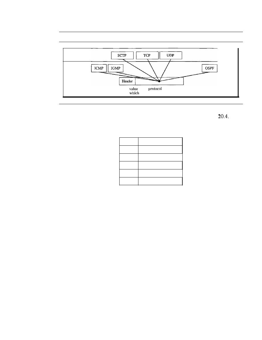
588
CHAPTER 20
NETWORK lAYER: INTERNET PROTOCOL
Figure 20.8
Protocol field and encapsulated data
Transport layer
Network layer
The
of the
field defines
to
protocol the data belong.
The value of this field for each higher-level protocol is shown in Table
Table 20.4
Protocol values
Value
Protocol
1
ICMP
2
IGMP
6
TCP
17
UDP
89
OSPF
o
Checksum.
The checksum concept and its calculation are discussed later in this
chapter.
o
Source address.
This 32-bit field defines the IPv4 address of the source. This field
must remain unchanged during the time the IPv4 datagram travels from the source
host to the destination host.
o
Destination address.
This 32-bit field defines the IPv4 address of the destination.
This field must remain unchanged during the time the IPv4 datagram travels from
the source host to the destination host.
Example 20.1
An IPv4 packet has arrived with the first 8 bits as shown:
01000010
The receiver discards the packet. Why?
Solution
There is an elTOr in this packet. The 4 leftmost bits (0100) show the version, which is correct. The
next 4 bits (0010) show an invalid header length (2
x
4
=
8). The minimum number of bytes in the
header must be 20. The packet has been corrupted in transmission.

SECTION 20.2
IPv4
589
Example 20.2
In an IPv4 packet, the value of HLEN is 1000 in binary. How many bytes of options are being
carried by this packet?
Solution
The HLEN value is 8, which means the total number of bytes in the header is 8 x 4, or 32 bytes.
The first 20 bytes are the base header, the next 12 bytes are the options.
Example 20.3
In an IPv4 packet, the value of HLEN is 5, and the value of the total length field is Ox0028. How
many bytes of data are being carried by this packet?
Solution
The HLEN value is 5, which means the total number of bytes in the header is 5 x 4, or 20 bytes (no
options). The total length is 40 bytes, which means the packet is carrying 20 bytes of data (40- 20).
Example 20.4
An IPv4 packet has arrived with the first few hexadecimal digits as shown.
Ox45000028000100000102 ...
How many hops can this packet travel before being dropped? The data belong to what upper-layer
protocol?
Solution
To find the time-to-live field, we skip 8 bytes (16 hexadecimal digits). The time-to-live field is the
ninth byte, which is 01. This means the packet can travel only one hop. The protocol field is the
next byte (02), which means that the upper-layer protocol is IGMP (see Table 20.4).
Fragmentation
A datagram can travel through different networks. Each router decapsulates the IPv4
datagram from the frame it receives, processes it, and then encapsulates it in another
frame. The format and size of the received frame depend on the protocol used by the
physical network through which the frame has just traveled. The format and size of
the sent frame depend on the protocol used by the physical network through which the
frame is going to travel. For example, if a router connects a LAN to a WAN, it receives
a frame in the LAN format and sends a frame in the WAN format.
Maximum Transfer Unit (MTU)
Each data link layer protocol has its own frame format in most protocols. One of the
fields defined in the format is the maximum size of the data field. In other words, when
a datagram is encapsulated in a frame, the total size of the datagram must be less than
this maximum size, which is defined by the restrictions imposed by the hardware and
software used in the network (see Figure 20.9).
The value of the MTU depends on the physical network protocol. Table 20.5 shows
the values for some protocols.
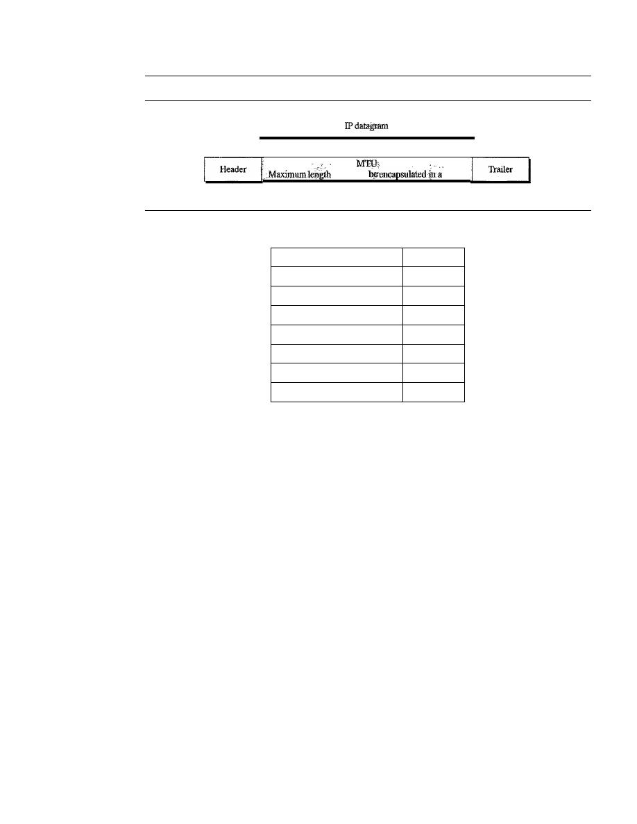
590
CHAPTER 20
NETWORK LAYER: INTERNET PROTOCOL
Figure 20.9
Maximum transfer unit (MTU)
of data to
frame
Frame
Table 20.5
MTUs for some networks
Protocol
MTU
Hyperchannel
65,535
Token Ring (16 Mbps)
17,914
Token Ring (4 Mbps)
4,464
FDDI
4,352
Ethernet
1,500
X.25
576
PPP
296
To make the IPv4 protocol independent of the physical network, the designers
decided to make the maximum length of the IPv4 datagram equal to 65,535 bytes. This
makes transmission more efficient if we use a protocol with an MTU of this size. How-
ever, for other physical networks, we must divide the datagram to make it possible to
pass through these networks. This is called fragmentation.
The source usually does not fragment the IPv4 packet. The transport layer will
instead segment the data into a size that can be accommodated by IPv4 and the data
link layer in use.
When a datagram is fragmented, each fragment has its own header with most of
the fields repeated, but with some changed. A fragmented datagram may itself be frag-
mented if it encounters a network with an even smaller MTU. In other words, a data-
gram can be fragmented several times before it reaches the final destination.
In IPv4, a datagram can be fragmented by the source host or any router in the path
although there is a tendency to limit fragmentation only at the source. The reassembly of
the datagram, however, is done only by the destination host because each fragment
becomes an independent datagram. Whereas the fragmented datagram can travel through
different routes, and we can never control or guarantee which route a fragmented data-
gram may take, all the fragments belonging to the same datagram should finally arrive at
the destination host. So it is logical to do the reassembly at the final destination. An even
stronger objection to reassembling packets during the transmission is the loss of effi-
ciency it incurs.
When a datagram is fragmented, required parts of the header must be copied by all
fragments. The option field mayor may not be copied, as we will see in the next section.
The host or router that fragments a datagram must change the values of three fields:

SECTION 20.2
IPv4
591
flags, fragmentation offset, and total length. The rest of the fields must be copied. Of
course, the value of the checksum must be recalculated regardless of fragmentation.
Fields Related to Fragmentation
The fields that are related to fragmentation and reassembly of an IPv4 datagram are the
identification, flags, and fragmentation offset fields.
o
Identification. This 16-bit field identifies a datagram originating from the source
host. The combination of the identification and source IPv4 address must uniquely
define a datagram as it leaves the source host. To guarantee uniqueness, the IPv4
protocol uses a counter to label the datagrams. The counter is initialized to a posi-
tive number. When the IPv4 protocol sends a datagram, it copies the current value
of the counter to the identification field and increments the counter
1. As long as
the counter is kept in the main memory, uniqueness is guaranteed. When a data-
gram is fragmented, the value in the identification field is copied to all fragments.
In other words, all fragments have the same identification number, the same as the
original datagram. The identification number helps the destination in reassembling
the datagram.
It
knows that all fragments having the same identification value must
be assembled into one datagram.
o
Flags. This is a 3-bit field. The first bit is reserved. The second bit is called the
do
notfragment
bit.
If
its value is
1,
the machine must not fragment the datagram. If it
cannot pass the datagram through any available physical network, it discards the
datagram and sends an ICMP error message to the source host (see Chapter 21).
If
its value is 0, the datagram can be fragmented if necessary. The third bit is called
the
more fragment
bit.
If
its value is 1, it means the datagram is not the last frag-
ment; there are more fragments after this one.
If
its value is 0, it means this is the
last or only fragment (see Figure 20.10).
Figure 20.10
Flags used in fragmentation
D: Donat fragment
M: More fragments
o
Fragmentation offset. This 13-bit field shows the relative position of this frag-
ment with respect to the whole datagram.
It
is the offset of the data in the original
datagram measured in units of 8 bytes. Figure 20.11 shows a datagram with a data
size of 4000 bytes fragmented into three fragments.
The bytes in the original datagram are numbered 0 to 3999. The first fragment
carries bytes 0 to 1399. The offset for this datagram is 0/8
=
O. The second frag-
ment carries bytes 1400 to 2799; the offset value for this fragment is 1400/8
=
175.
Finally, the third fragment carries bytes 2800 to 3999. The offset value for this
fragment is 2800/8
=
350.
Remember that the value of the offset is measured in units of 8 bytes. This is
done because the length of the offset field is only 13 bits and cannot represent a
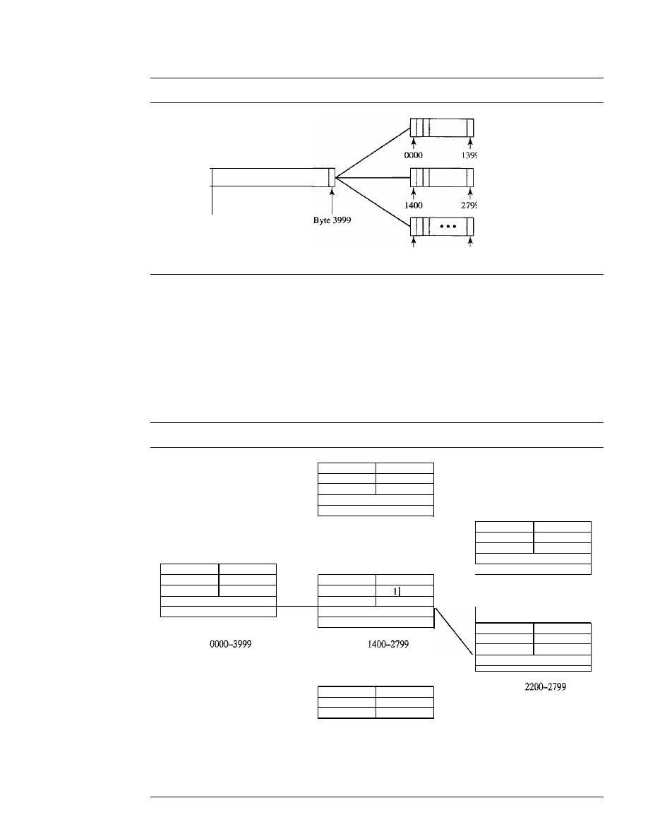
592
CHAPTER 20
NETWORK LAYER: INTERNET PROTOCOL
Figure 20.11
Fragmentation example
Byte 0000
Offset
= 0000/8 =
0
•••
Offset
=
0000/8
=
0
Offset
=
1400/8
=
175
Offset
= 2800/8
=
350
2800
3999
sequence of bytes greater than 8191. This forces hosts or routers that fragment data-
grams to choose a fragment size so that the first byte number is divisible by 8.
Figure 20.12 shows an expanded view of the fragments in Figure 20.11.
Notice the value of the identification field is the same in all fragments. Notice the
value of the flags field with the more bit set for all fragments except the last. Also,
the value of the offset field for each fragment is shown.
Figure 20.12
Detailedfragmentation example
I
I
1420
14,567
I
111
000
I
Bytes 0000-1399
I
I
820
14,567
I
111
175
Fragment 1
I
I
I
4020
1/
14,567
I
101
000
I
I
1420
Bytes 1400-2199
I
14,567
I I
175
I
Fragment 2.1
I
I
620
Bytes
Bytes
14,567
I III
275
I
Fragment 2
Original datagram
I
I
1220
Bytes
14,567
I
101' 350
Fragment 2.2
I
Bytes 2800-3999
Fragment 3

SECTION 20.2
IPv4
593
The figure also shows what happens if a fragment itself is fragmented. In this
case the value of the offset field is always relative to the original datagram. For
example, in the figure, the second fragment is itself fragmented later to two frag-
ments of 800 bytes and 600 bytes, but the offset shows the relative position of the
fragments to the original data.
It
is obvious that even if each fragment follows a different path and arrives out
of order, the final destination host can reassemble the original datagram from the
fragments received (if none of them is lost) by using the following strategy:
1. The first fragment has an offset field value of zero.
2. Divide the length of the first fragment by 8. The second fragment has an offset
value equal to that result.
3. Divide the total length of the first and second fragments by 8. The third fragment
has an offset value equal to that result.
4. Continue the process. The last fragment has a
more
bit value of O.
Example 20.5
A packet has arrived with an
M
bit value of O. Is this the first fragment, the last fragment, or a
middle fragment? Do we know if the packet was fragmented?
Solution
If the
M
bit is 0, it means that there are no more fragments; the fragment is the last one. However,
we cannot say if the original packet was fragmented or not. A nonfragmented packet is consid-
ered the last fragment.
Example 20.6
A packet has arrived with an
M
bit value of 1. Is this the first fragment, the last fragment, or a
middle fragment? Do we know if the packet was fragmented?
Solution
If the
M
bit is 1, it means that there is at least one more fragment. This fragment can be the first
one or a middle one, but not the last one. We don't know if it is the first one or a middle one; we
need more information (the value of the fragmentation offset). See Example 20.7.
Example 20.7
A packet has arrived with an
M
bit value of 1 and a fragmentation offset value of O. Is this the first
fragment, the last fragment, Or a middle fragment?
Solution
Because the
M
bit is l, it is either the first fragment or a middle one. Because the offset value is 0,
it is the first fragment.
Example 20.8
A packet has arrived in which the offset value is 100. What is the number of the first byte? Do we
know the number of the last byte?

594
CHAPTER
20
NETWORK LAYER: INTERNET PROTOCOL
Solution
To find the number of the first byte, we multiply the offset value by 8. This means that the first
byte number is 800. We cannot determine the number of the last byte unless we know the length
of the data.
Example 20.9
A packet has arrived in which the offset value is 100, the value of HLEN is 5, and the value of the
tota1length field is 100. What are the numbers of the first byte and the last byte?
Solution
The first byte number is 100 x 8
=
800. The total length is 100 bytes, and the header length is
20 bytes (5 x 4), which means that there are 80 bytes in this datagram. If the first byte number
is 800, the last byte number must be 879.
Checksum
We discussed the general idea behind the checksum and how it is calculated in Chapter 10.
The implementation of the checksum in the IPv4 packet follows the same principles. First,
the value of the checksum field is set to O. Then the entire header is divided into 16-bit
sections and added together. The result (sum) is complemented and inserted into the
checksum field.
The checksum in the IPv4 packet covers only the header, not the data. There are two
good reasons for this. First, all higher-level protocols that encapsulate data in the IPv4
datagram have a checksum field that covers the whole packet. Therefore, the checksum
for the IPv4 datagram does not have to check the encapsulated data. Second, the header
of the IPv4 packet changes with each visited router, but the data do not. So the checksum
includes only the part that has changed. If the data were included, each router must recal-
culate the checksum for the whole packet, which means an increase in processing time.
Example 20.10
Figure 20.13 shows an example of a checksum calculation for an IPv4 header without options.
The header is divided into 16-bit sections. All the sections are added and the sum is comple-
mented. The result is inserted in the checksum field.
Options
The header of the IPv4 datagram is made of two parts: a fixed palt and a variable part.
The fixed part is 20 bytes long and was discussed in the previous section. The variable
part comprises the options that can be a maximum of 40 bytes.
Options, as the name implies, are not required for a datagram. They can be used for
network testing and debugging. Although options are not a required part of the IPv4
header, option processing is required of the IPv4 software. This means that all imple-
mentations must be able to handle options if they are present in the header.
The detailed discussion of each option is beyond the scope of this book. We give
the taxonomy of options in Figure 20.14 and briefly explain the purpose of each.
No Operation
A no-operation option is a I-byte option used as a filler between options.
SECTION 20.2
IPv4
595
Figure 20.13
Example of checksum calculation in IPv4
4
I
5
I
0
28
1
o
I
0
4
I
17
10.12.14.5
12.6.7.9
4,5, and 0
4
5
0
0
28
0
0
1
C
1
0
0
0
1
o
and 0
0
0
0
0
4 and 17
0
4
1
1
0
0
0
0
0
10.12
0
A
0
C
14.5
0
E
0
5
12.6
0
C
0
6
7.9
0
7
0
9
Sum
7
4
4
E
Checksum
8
B
B
1
Figure 20.14
Taxonomy of options in IPv4
Single-byte
No operation
End of option
Options
Multiple-byte
Record route
Strict source route
Loose source route
Timestamp
End of Option
An
end-of-option option is a I-byte option used for padding at the end of the option
field.
It,
however, can only be used as the last option.
Record Route
A
record route option is used to record the Internet routers that handle the datagram.
It
can list up to nine router addresses.
It
can be used for debugging and management
purposes.
Strict Source Route
A
strict source route option is used by the source to predetermine a route for the data-
gram as it travels through the Internet. Dictation of a route by the source can be useful

596
CHAPTER 20
NETWORK LAYER: INTERNET PROTOCOL
for several purposes. The sender can choose a route with a specific type of service, such
as minimum delay or maximum throughput. Alternatively, it may choose a route that is
safer or more reliable for the sender's purpose. For example, a sender can choose a route
so that its datagram does not travel through a competitor's network.
If
a datagram specifies a strict source route, all the routers defined in the option
must be visited by the datagram. A router must not be visited if its IPv4 address is not
listed in the datagram.
If
the datagram visits a router that is not on the list, the datagram
is discarded and an error message is issued.
If
the datagram arrives at the destination
and some of the entries were not visited,
it
will also be discarded and an error message
issued.
Loose Source Route
A loose source route option is similar to the strict source route, but it is less rigid. Each
router in the list must be visited, but the datagram can visit other routers as well.
Timestamp
A timestamp option is used to record the time of datagram processing by a router. The
time is expressed in milliseconds from midnight, Universal time or Greenwich mean
time. Knowing the time a datagram is processed can help users and managers track the
behavior of the routers in the Internet. We can estimate the time it takes for a datagram
to go from one
to another. We say estimate because, although all routers may use
Universal time, their local clocks may not be synchronized.
20.3
IPv6
The network layer protocol in the TCPIIP protocol suite is currently IPv4 (Internet-
working Protocol, version 4). IPv4 provides the host-to-host communication between
systems in the Internet. Although IPv4 is well designed, data communication has
evolved since the inception of IPv4 in the 1970s. IPv4 has some deficiencies (listed
below) that make it unsuitable for the fast-growing Internet.
o
Despite all short-term solutions, such as subnetting, classless addressing, and NAT,
address depletion is still a long-term problem in the Internet.
o
The Internet must accommodate real-time audio and video transmission. This type
of transmission requires minimum delay strategies and reservation of resources not
provided in the IPv4 design.
o
The Internet must accommodate encryption and authentication of data for some
applications. No encryption or authentication is provided by IPv4.
To overcome these deficiencies, IPv6 (Internetworking Protocol, version 6), also
known as IPng (Internetworking Protocol, next generation), was proposed and is
now a standard. In IPv6, the Internet protocol was extensively modified to accommo-
date the unforeseen growth of the Internet. The format and the length of the IP address
were changed along with the packet format. Related protocols, such as ICMP, were also
modified. Other protocols in the network layer, such as ARP, RARP, and IGMP, were

SECTION 20.3
IPv6
597
either deleted or included in the ICMPv6 protocol (see Chapter 21). Routing protocols,
such as RIP and OSPF (see Chapter 22), were also slightly modified to accommodate
these changes. Communications experts predict that IPv6 and its related protocols will
soon replace the current IP version. In this section first we discuss IPv6. Then we explore
the strategies used for the transition from version 4 to version 6.
The adoption of IPv6 has been slow. The reason is that the original motivation for
its development, depletion of IPv4 addresses,
been remedied by short-term strategies
such as classless addressing and NAT. However, the fast-spreading use of the Internet,
and new services such as mobile IP, IP telephony, and IP-capable mobile telephony, may
eventually require the total replacement of IPv4 with IPv6.
Advantages
The next-generation IP, or IPv6, has some advantages over IPv4 that can be summarized
as follows:
o
Larger address space.
An IPv6 address is 128 bits long, as we discussed in Chap-
ter 19. Compared with the 32-bit address of IPv4, this is a huge (2
96
)
increase in
the address space.
o
Better header format.
IPv6 uses a new header format in which options are sepa-
rated from the base header and inserted, when needed, between the base header
and the upper-layer data. This simplifies and speeds up the routing process because
most of the options do not need to be checked by routers.
o
New options.
IPv6 has new options to allow for additional functionalities.
o
Allowance for extension.
IPv6 is designed to allow the extension of the protocol if
required by new technologies or applications.
o
Support for resource allocation.
In IPv6, the type-of-service field has been
removed, but a mechanism (calledjlow label) has been added to enable the source
to request special handling of the packet. This mechanism can be used to support
traffic such as real-time audio and video.
o
Support for more security.
The encryption and authentication options in IPv6
provide confidentiality and integrity of the packet.
Packet Format
The IPv6 packet is shown
in
Figure 20.15. Each packet is composed of a mandatory base
header followed by the payload. The payload consists of two parts: optional extension
headers and data from an upper layer. The base header occupies 40 bytes, whereas the
extension headers and data from the upper layer contain up to 65,535 bytes of information.
Base Header
Figure 20.16 shows the
base header
with its eight fields.
These fields are as follows:
o
Version.
This 4-bit field defines the version number of the IP. For IPv6, the value is 6.
o
Priority.
The 4-bit priority field defines the priority of the packet with respect to
traffic congestion. We will discuss this field later.
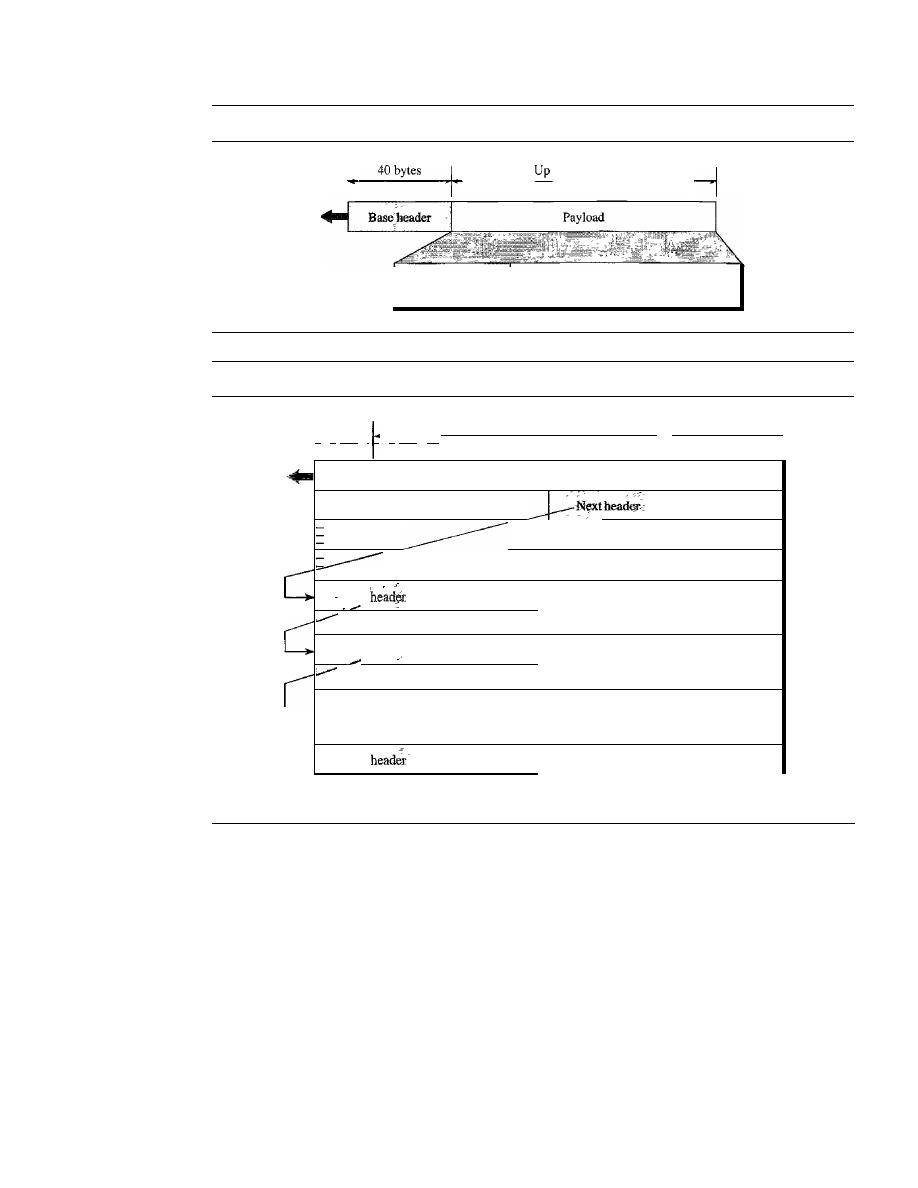
598
CHAPTER 20
NETWORK LAYER: INTERNET PROTOCOL
Figure 20.15
IPv6 datagram header and payload
1'
'
_to_65_,5_3_5_bY
_te_s
Extension headers
(optional)
Figure 20.16
Format of an IPv6 datagram
Data packet from upper layer
I'
4 bits
I
4 bits
'1-
8 bits
8 bits
8
bits
VER
I
PRl
I
Flow label
Payload length
I
Hop limit
Source address
Destination address
-
I
I
Next
Header length
Next header
I
Header length
I
•
•
·
··
•
L
I
I
Next
Header length
o
Flow label. The flow label is a 3-byte (24-bit) field that is designed to provide
special handling for a particular flow of data. We will discuss this field later.
o
Payload length. The 2-byte payload length field defines the length of the IP data-
gram excluding the base header.
o
Next header. The next header is an 8-bit field defining the header that follows the
base header in the datagram. The next header is either one of the optional exten-
sion headers used by IP or the header of an encapsulated packet such as UDP or
TCP. Each extension header also contains this field. Table 20.6 shows the values of
next headers. Note that this field in version 4 is called the protocol.
o
Hop
limit.
This 8-bit hop
limit
field serves the same purpose as the TIL field in IPv4.
o
Source address. The source address field is a 16-byte (128-bit) Internet address
that identifies the original source of the datagram.

SECTION 20.3
IPv6
599
Table 20.6
Next header codes for IPv6
Code
Next Header
0
Hop-by-hop option
2
ICMP
6
TCP
17
UDP
43
Source routing
44
Fragmentation
50
Encrypted security payload
51
Authentication
59
Null (no next header)
60
Destination option
o
Destination address.
The destination address field is a 16-byte (128-bit) Internet
address that usually identifies the final destination of the datagram. However, if
source routing is used, this field contains the address of the next router.
Priority
The priority field of the IPv6 packet defines the priority of each packet with respect to
other packets from the same source. For example, if one of two consecutive datagrams
must be discarded due to congestion, the datagram with the lower
packet priority
will
be discarded. IPv6 divides traffic into two broad categories: congestion-controlled and
noncongestion-controlled.
Congestion-Controlled Traffic
If a source adapts itself to traffic slowdown when
there is congestion, the traffic is referred to as
congestion-controlled traffic.
For
example, TCP, which uses the sliding window protocol, can easily respond to traffic.
In
congestion-controlled traffic,
it
is understood that packets may arrive delayed, lost, or
out of order. Congestion-controlled data are assigned priorities from 0 to 7, as listed in
Table 20.7. A priority of 0 is the lowest; a priority of 7 is the highest.
Table 20.7
Priorities for congestion-controlled traffic
Priority
Meaning
0
No specific traffic
1
Background data
2
Unattended data traffic
3
Reserved
4
Attended bulk data traffic
5
Reserved
6
Interactive traffic
7
Control traffic

600
CHAPTER 20
NETWORK LAYER: INTERNET PROTOCOL
The priority descriptions are as follows:
o
No specific traffic. A priority of 0 is assigned to a packet when the process does
not define a priority.
o
Background data. This group (priority 1) defines data that are usually delivered
in the background. Delivery of the news is a good example.
o
Unattended data traffic.
If
the user is not waiting (attending) for the data to be
received, the packet will be given a priority of 2. E-mail belongs to this group. The
recipient of an e-mail does not know when a message has arrived. In addition, an
e-mail is usually stored before it is forwarded. A little bit of delay is of little
consequence.
o
Attended
bulk
data traffic. A protocol that transfers data while the user is waiting
(attending) to receive the data (possibly with delay) is given a priority of 4. FTP
and HTTP belong to this group.
o
Interactive traffic. Protocols such as TELNET that need user interaction are
assigned the second-highest priority (6) in this group.
o
Control traffic. Control traffic is given the highest priority (7). Routing protocols
such as OSPF and RIP and management protocols such as SNMP have this priority.
Noncongestion-Controlled Traffic
This refers to a type of traffic that expects mini-
mum delay. Discarding of packets is not desirable. Retransmission in most cases is
impossible. In other words, the source does not adapt itself to congestion. Real-time
audio and video are examples of this type of traffic.
Priority numbers from 8 to 15 are assigned to noncongestion-controlled traffic.
Although there are not yet any particular standard assignments for this type of data, the
priorities are usually based on how much the quality of received data is affected by the
discarding of packets. Data containing less redundancy (such as low-fidelity audio or
video) can be given a higher priority (15). Data containing more redundancy (such as
high-fidelity audio or video) are given a lower priority (8). See Table 20.8.
Table 20.8
Priorities for noncongestion-controlled traffic
Priority
Meaning
8
Data with greatest redundancy
.. .
. ,
.
15
Data with least redundancy
Flow Label
A sequence of packets, sent from a particular source to a particular destination, that needs
special handling by routers is called a
flow of packets. The combination of the source
address and the value of the
flow label uniquely defines a flow of packets.
To a router, a flow is a sequence of packets that share the same characteristics, such
as traveling the same path, using the same resources, having the same kind of security,
and so on. A router that supports the handling of flow labels has a flow label table. The
table has an entry for each active flow label; each entry defines the services required by

SECTION 20.3
IPv6
601
the corresponding flow label. When the router receives a packet, it consults its flow
label table to find the corresponding entry for the flow label value defined in the packet.
It
then provides the packet with the services mentioned in the entry. However, note that
the flow label itself does not provide the information for the entries of the flow label
table; the information is provided by other means such as the hop-by-hop options or
other protocols.
In its simplest form, a flow label can be used to speed up the processing of a packet
by a router. When a router receives a packet, instead of consulting the routing table and
going through a routing algorithm to define the address of the next hop, it can easily
look in a flow label table for the next hop.
In its more sophisticated form, a flow label can be used to support the transmission of
real-time audio and video. Real-time audio or video, particularly in digital form, requires
resources such as high bandwidth, large buffers, long processing time, and so on. A
process can make a reservation for these resources beforehand to guarantee that real-time
data will not be delayed due to a lack of resources. The use of real-time data and the
reservation of these resources require other protocols such as Real-Time Protocol (RTP)
and Resource Reservation Protocol (RSVP) in addition to IPv6.
To allow the effective use of flow labels, three rules have been defined:
1. The flow label is assigned to a packet by the source host. The label is a random
number between 1 and 2
24
-
1. A source must not reuse a flow label for a new flow
while the existing flow is still active.
2.
If
a host does not support the flow label, it sets this field to zero.
If
a router does not
support the flow label,
it
simply ignores it.
3. All packets belonging to the same flow have the same source, same destination,
same priority, and same options.
Comparison Between IPv4 and IPv6 Headers
Table 20.9 compares IPv4 and IPv6 headers.
Table 20.9
Comparison between IPv4 and IPv6 packet headers
Comparison
1. The header length field is eliminated in IPv6 because the length of the header is fixed in
this version.
2. The service type field is eliminated in IPv6. The priority and flow label fields together take
over the function of the service type field.
3. The total length field is eliminated in IPv6 and replaced by the payload length field.
4. The identification, flag, and offset fields are eliminated from the base header in IPv6. They
are included in the fragmentation extension header.
5. The TTL field is called hop limit in IPv6.
6. The protocol field is replaced by the next header field.
7. The header checksum is eliminated because the checksum is provided by upper-layer
protocols; it is therefore not needed at this level.
8. The option fields in IPv4 are implemented as extension headers in IPv6.
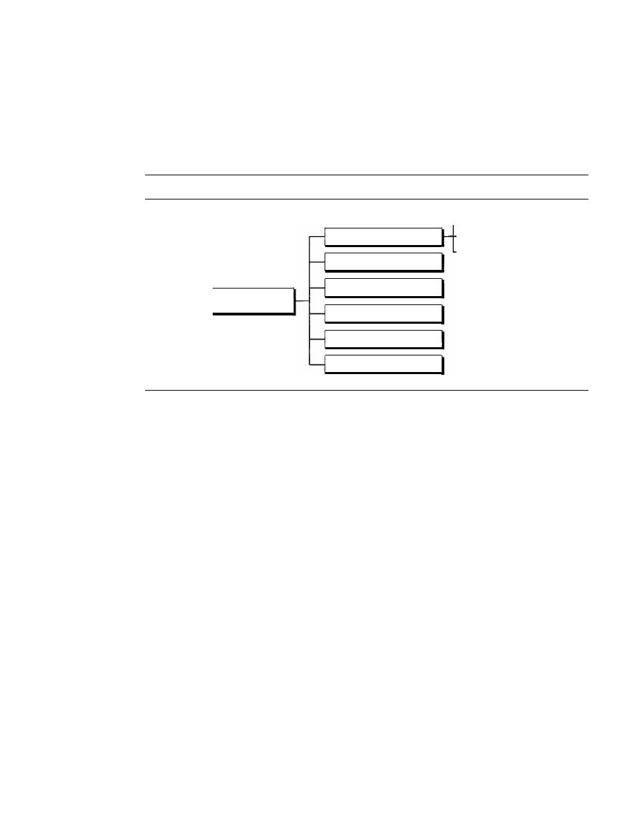
602
CHAPTER 20
NETWORK LAYER: INTERNET PROTOCOL
Extension Headers
The length of the base header is fixed at 40 bytes. However, to give greater functionality
to the IP datagram, the base header can be followed by up to six
extension headers.
Many of these headers are options in IPv4. Six types of extension headers have been
defined, as shown in Figure 20.17.
Figure 20.17
Extension header types
Pad I
Extension
headers
Hop-by-hop option
Source routing
Fragmentation
Authentication
Encrypted security payload
Destination option
PadN
Jumbo payload
Hop-by-Hop Option
The
hop-by-hop option
is used when the source needs to pass information to all routers
visited by the datagram. So far, only three options have been defined:
Padl, PadN,
and
jumbo payload.
The Padl option is 1 byte long and is designed for alignment pur-
poses. PadN is similar in concept to Padi. The difference is that PadN is used when 2 or
more bytes is needed for alignment. The jumbo payload option is used to define a pay-
load longer than 65,535 bytes.
Source Routing
The source routing extension header combines the concepts of the
strict source route and the loose source route options of IPv4.
Fragmentation
The concept of
fragmentation
is the same as that in IPv4. However, the place where
fragmentation occurs differs. In IPv4, the source or a router is required to fragment if
the size of the datagram is larger than the MTU of the network over which the datagram
travels. In IPv6, only the original source can fragment. A source must use a
path
MTU
discovery technique
to find the smallest MTU supported by any network on the path.
The source then fragments using this knowledge.
Authentication
The
authentication
extension header has a dual purpose: it validates the message sender
and ensures the integrity of data. We discuss this extension header when we discuss net-
work security in Chapter 31.
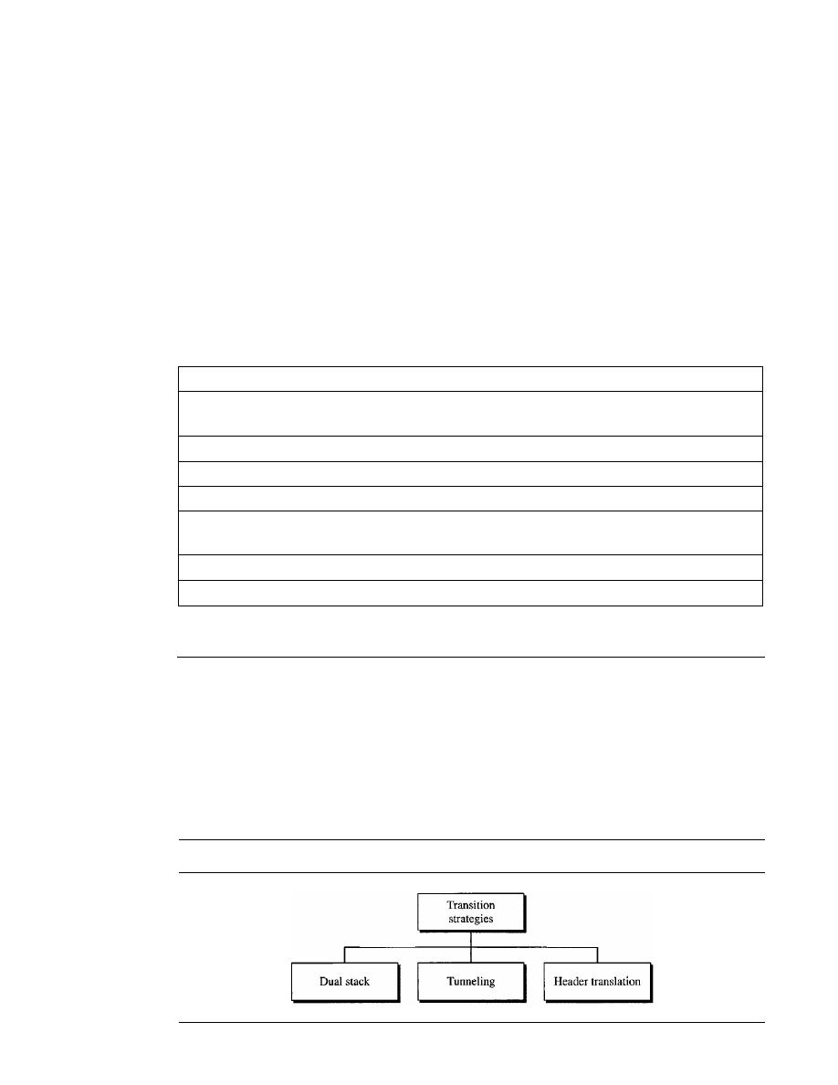
SECTION 20.4
TRANSITION FROM IPv4 TO IPv6
603
Encrypted Security Payload
The encrypted security payload (ESP) is an extension that provides confidentiality
and guards against eavesdropping. We discuss this extension header in Chapter 31.
Destination Option
The destination option is used when the source needs to pass
information to the destination only. Intermediate routers are not permitted access to this
information.
Comparison Between IPv4 Options and IPv6 Extension Headers
Table 20.10 compares the options in IPv4 with the extension headers in IPv6.
Table 20.10
Comparison between IPv4 options and IPv6 extension headers
Comparison
1.
The no-operation and end-of-option options in IPv4 are replaced by Padl and PadN
options in IPv6.
2. The record route option is not implemented in IPv6 because it was not used.
3. The timestamp option is not implemented because it was not used.
4. The source route option is called the source route extension header in IPv6.
5. The fragmentation fields in the base header section of IPv4 have moved to the fragmentation
extension header in IPv6.
6. The authentication extension header is new in IPv6.
7. The encrypted security payload extension header is new in IPv6.
20.4
TRANSITION FROM IPv4 TO IPv6
Because of the huge number of systems on the Internet, the transition from IPv4
to IPv6 cannot happen suddenly. It takes a considerable amount of time before every
system in the Internet can move from IPv4 to IPv6. The transition must be smooth to
prevent any problems between IPv4 and IPv6 systems. Three strategies have been
devised by the !ElF to help the transition (see Figure 20.18).
Figure 20.18
Three transition strategies
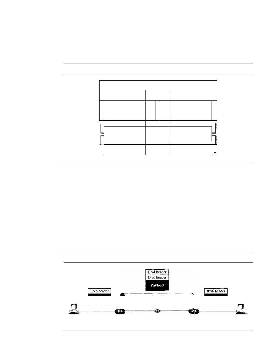
604
CHAPTER 20
NETWORK LAYER: INTERNET PROTOCOL
Dual Stack
It
is recommended that all hosts, before migrating completely to version 6, have a dual
stack of protocols. In other words, a station must run IPv4 and IPv6 simultaneously until
all the Internet uses IPv6. See Figure 20.19 for the layout of a dual-stack configuration.
Figure 20.19
Dual stack
o IPv6 system
Transport and
application layers
IPv4
IPv6
Underlying
LAN or WAN
technology
m
To IPv4 syste
To determine which version to use when sending a packet to a destination, the source
host queries the DNS. If the DNS returns an IPv4 address, the source host sends an IPv4
packet.
If
the DNS returns an IPv6 address, the source host sends an IPv6 packet.
Tunneling
Thnneling is a strategy used when two computers using IPv6 want to communicate
with each other and the packet must pass through a region that uses IPv4. To pass
through this region, the packet must have an IPv4 address. So the IPv6 packet is encap-
sulated in an IPv4 packet when it enters the region, and it leaves its capsule when it
exits the region. It seems as if the IPv6 packet goes through a tunnel at one end and
emerges at the other end. To make it clear that the IPv4 packet is carrying an IPv6
packet as data, the protocol value is set to 41. Tunneling is shown in Figure 20.20.
Figure 20.20
Tunneling strategy
IPv6
IPv6
host
host
IPv4region
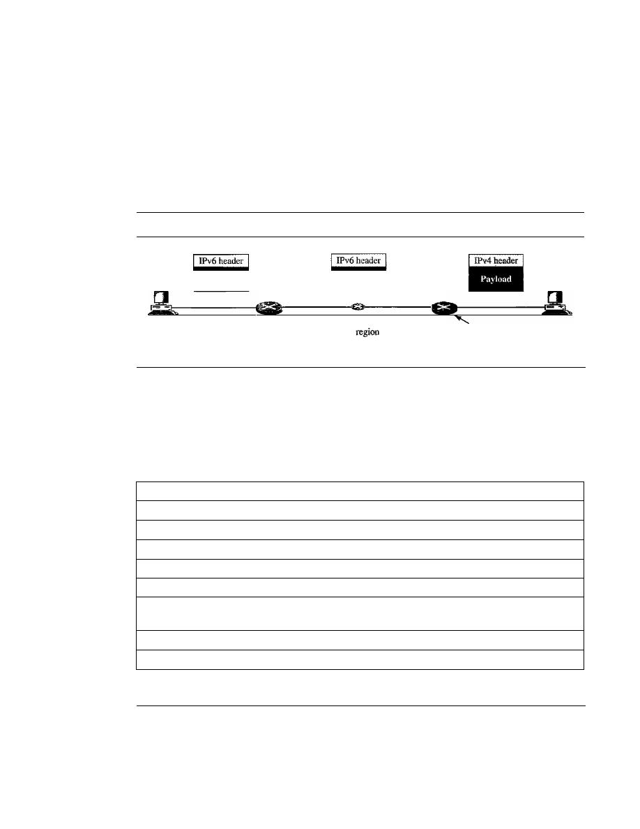
IPv6
SECTION 20.5
RECOMMENDED READING
605
Header Translation
Header translation is necessary when the majority of the Internet has moved to IPv6
but some systems still use IPv4. The sender wants to use IPv6, but the receiver does not
understand IPv6. Tunneling does not work in this situation because the packet must be
in the IPv4 format to be understood by the receiver. In this case, the header format must
be totally changed through header translation. The header of the IPv6 packet is con-
verted to an IPv4 header (see Figure 20.21).
Figure 20.21
Header translation strategy
IPv6
•
I
IPv4
host
host
Header
translation
done here
Header translation uses the mapped address to translate an IPv6 address to an IPv4
address. Table 20.11 lists some rules used in transforming an IPv6 packet header to an
IPv4 packet header.
Table 20.11
Header translation
Header Translation Procedure
1. The IPv6 mapped address is changed to an IPv4 address by extracting the rightmost 32 bits.
2. The value of the IPv6 priority field is discarded.
3. The type of service field in IPv4 is set to zero.
4. The checksum for IPv4 is calculated and inserted in the corresponding field.
5. The IPv6 flow label is ignored.
6. Compatible extension headers are converted to options and inserted in the IPv4 header.
Some may have to be dropped.
7. The length of IPv4 header is calculated and inserted into the corresponding field.
8. The total length of the IPv4 packet is calculated and inserted in the corresponding field.
20.5
RECOMMENDED READING
For more details about subjects discussed in this chapter, we recommend the following
books and sites. The items in brackets [...] refer to the reference list at the end of
the text.

606
CHAPTER 20
NETWORK LAYER: INTERNET PROTOCOL
Books
IPv4 is discussed in Chapter 8 of [For06], Chapter 3 of [Ste94J, Section 4.1 of [PD03],
Chapter 18 of [Sta04], and Section 5.6 of [Tan03]. IPv6 is discussed in Chapter 27 of
[For06] and [Los04].
Sites
o
www.ietforg/rfc.html Information about RFCs
RFCs
A discussion of IPv4 can be found in following RFCs:
760,781,791,815,1025,1063,1071,1141,1190, 1191, 1624,2113
A discussion of IPv6 can be found in the following RFCs:
1365,1550,1678,1680,1682,1683,1686,1688,1726, 1752, 1826, 1883, 1884, 1886, 1887,
1955,2080,2373,2452,2463,2465,2466,2472,2492,2545,2590
20.6
KEY TERMS
authentication
base header
best-effort delivery
codepoint
connectionless service
connection-oriented service
datagram
destination address
destination option
differentiated services
dual stack
encrypted security payload (ESP)
end-of-option option
extension header
flow label
fragmentation
fragmentation offset
header length
header translation
hop limit
hop-by-hop option
Internet Protocol (IP)
Internet Protocol, next generation (IPng)
Internet Protocol version 4 (IPv4)
Internet Protocol version 6 (IPv6)
jumbo payload
loose source route option
maximum transfer unit (MTU)
next header
noncongestion-controlled traffic
no-operation option
packet priority
Padl
PadN
path MTU discovery technique
precedence

record route option
service type
source address
strict source route option
SECTION 20.8
PRACTICE SET
607
time to live
timestamp option
tunneling
type of service (TOS)
20.7
SUMMARY
o
IPv4 is an unreliable connectionless protocol responsible for source-to-destination
delivery.
o
Packets in the IPv4 layer are called datagrams. A datagram consists of a header
(20 to 60 bytes) and data. The maximum length of a datagram is 65,535 bytes.
o
The MTU is the maximum number of bytes that a data link protocol can encapsulate.
MTUs vary from protocol to protocol.
o
Fragmentation is the division of a datagram into smaller units to accommodate the
MTU of a data link protocol.
o
The IPv4 datagram header consists of a fixed, 20-byte section and a variable options
section with a maximum of 40 bytes.
o
The options section of the IPv4 header is used for network testing and debugging.
o
The six IPv4 options each have a specific function. They are as follows: filler
between options for alignment purposes, padding, recording the route the datagram
takes, selection of a mandatory route by the sender, selection of certain routers that
must be visited, and recording of processing times at routers.
o
IPv6, the latest version of the Internet Protocol, has a 128-bit address space, a revised
header format, new options, an allowance for extension, support for resource
allocation, and increased security measures.
o
An IPv6 datagram is composed of a base header and a payload.
o
Extension headers add functionality to the IPv6 datagram.
o
Three strategies used to handle the transition from version 4 to version 6 are dual
stack, tunneling, and header translation.
20.8
PRACTICE SET
Review Questions
1. What is the difference between the delivery of a frame in the data link layer and the
delivery of a packet in the network layer?
2. What is the difference between connectionless and connection-oriented services?
Which type of service is provided by IPv4? Which type of service is provided by IPv6?
3. Define fragmentation and explain why the IPv4 and IPv6 protocols need to fragment
some packets. Is there any difference between the two protocols in this matter?

608
CHAPTER 20
NETWORK LAYER: INTERNET PROTOCOL
4. Explain the procedure for checksum calculation and verification in the IPv4 protocol.
What part of an IPv4 packet is covered in the checksum calculation? Why? Are
options, if present, included in the calculation?
5. Explain the need for options in IPv4 and list the options mentioned in this chapter
with a brief description of each.
6. Compare and contrast the fields in the main headers of IPv4 and IPv6. Make a table
that shows the presence or absence of each field.
7. Both IPv4 and IPv6 assume that packets may have different priorities or precedences.
Explain how each protocol handles this issue.
8. Compare and contrast the options in IPv4 and the extension headers in IPv6. Make
a table that shows the presence or absence of each.
9. Explain the reason for the elimination of the checksum in the IPv6 header.
10. List three transition strategies to move from IPv4 to IPv6. Explain the difference
between tunneling and dual stack strategies during the transition period. When is
each strategy used?
Exercises
11. Which fields of the IPv4 header change from router to router?
12. Calculate the HLEN (in IPv4) value if the total length is 1200 bytes, 1176 of which
is data from the upper layer.
13. Table 20.5 lists the MTUs for many different protocols. The MTUs range from 296
to 65,535. What would be the advantages of having a large MTU? What would be
the advantages of having a small MTU?
14. Given a fragmented datagram (in IPv4) with an offset of 120, how can you determine
the first and last byte numbers?
15. Can the value of the header length in an IPv4 packet be less than 5? When is it
exactly 5?
16. The value ofHLEN in an IPv4 datagram is 7. How many option bytes are present?
17. The size of the option field of an IPv4 datagram is 20 bytes. What is the value of
HLEN? What is the value in binary?
18. The value of the total length field in an IPv4 datagram is 36, and the value of the
header length field is 5. How many bytes of data is the packet carrying?
19. An IPv4 datagram is carrying 1024 bytes of data.
If
there is no option information,
what is the value of the header length field? What is the value of the total length
field?
20. A host is sending 100 datagrams to another host.
If
the identification number of the
first datagram is 1024, what is the identification number of the last (in IPv4)?
21.
An
IPv4 datagram arrives with fragmentation offset of 0 and an
M
bit (more fragment
bit) of O. Is this a first fragment, middle fragment, or last fragment?
22. An IPv4 fragment has arrived with an offset value of 100. How many bytes of data
were originally sent by the source before the data in this fragment?

SECTION 20.8
PRACTICE SET
609
23. An IPv4 datagram has arrived with the following information
in
the header (in
hexadecimal):
Ox45 00 00 54 00 03 58 50 20 06 00 00 7C 4E 03 02 B4 OE OF 02
a. Is the packet corrupted?
b. Are there any options?
c. Is the packet fragmented?
d. What is the size of the data?
e. How many more routers can the packet travel to?
f.
What is the identification number of the packet?
g. What is the type of service?
24. In an IPv4 datagram, the
M
bit is 0, the value of HLEN is 5, the value of total
length is 200, and the offset value is 200. What is the number of the first byte and
number of the last byte
in
this datagram? Is this the last fragment, the first fragment,
or a middle fragment?
Research Activities
25. Find out why there are two security protocols (AH and ESP)
in
IPv6.


CHAPTER 21
Network Layer: Address Mapping,
Error Reporting, and Multicasting
In Chapter 20 we discussed the Internet Protocol (IP) as the main protocol at the network
layer. IP was designed as a best-effort delivery protocol, but it lacks some features such
as flow control and error control.
It
is a host-to-host protocol using logical addressing.
To make IP more responsive to some requirements in today's intemetworking, we need
the help of other protocols.
We need protocols to create a mapping between physical and logical addresses.
IP packets use logical (host-to-host) addresses. These packets, however, need to be encap-
sulated in a frame, which needs physical addresses (node-to-node). We will see that a
protocol called ARP, the Address Resolution Protocol, is designed for this purpose. We
sometimes need reverse mapping-mapping a physical address to a logical address. For
example, when booting a diskless network or leasing an IP address to a host. Three pro-
tocols are designed for this purpose: RARP, BOOTp, and DHCP.
Lack of flow and error control in the Internet Protocol has resulted in another pro-
tocol, ICMP, that provides alerts.
It
reports congestion and some types of errors in the
network or destination host.
IP was originally designed for unicast delivery, one source to one destination. As the
Internet has evolved, the need for multicast delivery, one source to many destinations, has
increased tremendously. IGMP gives IP a multicast capability.
In this chapter, we discuss the protocols ARP, RARP, BOOTP, DHCP, and IGMP
in some detail. We also discuss ICMPv6, which will be operational when IPv6 is oper-
ational. ICMPv6 combines ARP, ICMP, and IGMP in one protocol.
21.1
ADDRESS MAPPING
An internet is made of a combination of physical networks connected by internetworking
devices such as routers. A packet starting from a source host may pass through several
different physical networks before finally reaching the destination host. The hosts and
routers are recognized at the network level by their logical (IP) addresses.
However, packets pass through physical networks to reach these hosts and routers.
At the physical level, the hosts and routers are recognized by their physical addresses.
611

612
CHAPTER
21
NETWORK LAYER: ADDRESS MAPPING, ERROR REPORTING, AND MULTICASTING
A physical address
is a local address. Its jurisdiction is a local network. It must be
unique locally, but is not necessarily unique universally. It is called a physical address
because it is usually (but not always) implemented in hardware. An example of a physical
address is the 48-bit MAC address in the Ethernet protocol, which is imprinted on the
NIC installed in the host or router.
The physical address and the logical address are two different identifiers. We need
both because a physical network such as Ethernet can have two different protocols at
the network layer such as IP and IPX (Novell) at the same time. Likewise, a packet at a
network layer such as IP may pass through different physical networks such as Ethernet
and LocalTalk (Apple).
This means that delivery of a packet to a host or a router requires two levels of
addressing: logical and physical. We need to be able to map a logical address to its cor-
responding physical address and vice versa. These can be done by using either static or
dynamic mapping.
Static mapping
involves in the creation of a table that associates a logical address
with a physical address. This table is stored in each machine on the network. Each machine
that knows, for example, the IP address of another machine but not its physical address
can look it up in the table. This has some limitations because physical addresses may
change in the following ways:
1. A machine could change its NIC, resulting in a new physical address.
2. In some LANs, such as LocalTalk, the physical address changes every time the
computer is turned on.
3. A mobile computer can move from one physical network to another, resulting in a
change in its physical address.
To implement these changes, a static mapping table must be updated periodically. This
overhead could affect network performance.
In
dynamic mapping
each time a machine knows one of the two addresses (logical
or physical), it can use a protocol to find the other one.
Mapping Logical to Physical Address: ARP
Anytime a host or a router has an IP datagram to send to another host or router, it has the
logical (IP) address of the receiver. The logical (IP) address is obtained from the DNS
(see Chapter 25) if the sender is the host or it is found in a routing table (see Chapter 22)
if the sender is a router. But the IP datagram must be encapsulated in a frame to be able to
pass through the physical network. This means that the sender needs the physical address
of the receiver. The host or the router sends an ARP query packet. The packet includes
the physical and IP addresses of the sender and the IP address of the receiver. Because
the sender does not know the physical address of the receiver, the query is broadcast
over the network (see Figure 21.1).
Every host or router on the network receives and processes the ARP query packet,
but only the intended recipient recognizes its IP address and sends back an ARP response
packet. The response packet contains the recipient's IP and physical addresses. The packet
is unicast directly to the inquirer by using the physical address received in the query
packet.
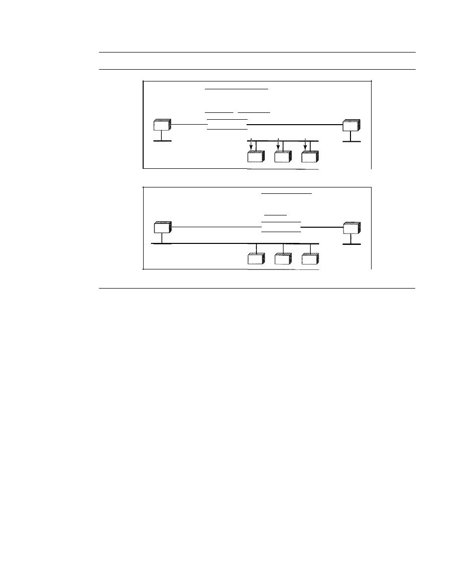
SECTION
21.1
ADDRESS MAPPING
613
Figure 21.1
ARP operation
Looking for physical address of a
node with IP address 141.23.56.23
Request
System A
a. ARP request is broadcast
System A
b. ARP reply is unicast
The node physical address
is A4:6E:F4:59:83:AB
Reply
System
B
System B
In Figure 21.1a, the system on the left (A) has a packet that needs to be delivered to
another system (B) with IP address 141.23.56.23. System A needs to pass the packet to
its data link layer for the actual delivery, but it does not know the physical address of
the recipient.
It
uses the services of ARP by asking the ARP protocol to send a broad-
cast ARP request packet to ask for the physical address of a system with an IF address
of 141.23.56.23.
This packet is received by every system on the physical network, but only system B
will answer it, as shown in Figure 21.1 b. System B sends an ARP reply packet that
includes its physical address. Now system A can send all the packets it has for this des-
tination by using the physical address it received.
Cache Memory
Using ARP is inefficient if system A needs to broadcast an ARP request for each IP
packet it needs to send to system B.
It
could have broadcast the IP packet itself. ARP
can be useful if the ARP reply is cached (kept in cache memory for a while) because a
system normally sends several packets to the same destination. A system that receives
an ARP reply stores the mapping in the cache memory and keeps it for 20 to 30 minutes
unless the space in the cache is exhausted. Before sending an ARP request, the system
first checks its cache to see if it can find the mapping.
Packet Format
Figure 21.2 shows the format of an ARP packet.
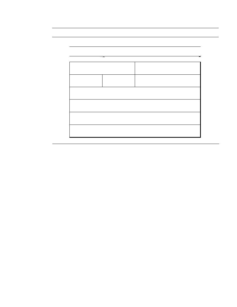
614
CHAPTER
21
NETWORK LAYER: ADDRESS MAPPING, ERROR REPORTING, AND MULTICASTING
Figure 21.2
ARP packet
32 bits
8 bits
l I
8 bits
16 bits
I
I
I
I
Hardware Type
Protocol Type
Hardware
Protocol
Operation
length
length
Request I, Reply 2
Sender hardware address
(For example, 6 bytes for Ethernet)
Sender protocol address
(For example, 4 bytes for IP)
Target hardware address
(For example, 6 bytes for Ethernet)
(It is not filled in a request)
Target protocol address
(For example, 4 bytes for IP)
Thc fields arc as follows:
o
Hardware type. This is a 16-bit field defining the type of the network on which
ARP is running. Each LAN has been assigned an integer based on its type. For
example, Ethernet is given type 1. ARP can be used on any physical network.
o
Protocol type. This is a 16-bit field defining the protocol. For example, the value
of this field for the IPv4 protocol is 0800
16,
ARP can be used with any higher-level
protocol.
o
Hardware length. This is an 8-bit field defining the length of the physical address
in bytes. For example, for Ethernet the value is 6.
o
Protocol length. This is an 8-bit field defining the length of the logical address in
bytes. For example, for the IPv4 protocol the value is 4.
o
Operation. This is a 16-bit field defining the type of packet. Two packet types are
defined: ARP request (1) andARP reply (2).
o
Sender hardware address. This is a variable-length field defining the physical
address of the sender. For example, for Ethernet this field is 6 bytes long.
o
Sender protocol address. This is a variable-length field defining the logical (for
example, IP) address of the sender. For the IP protocol, this field is 4 bytes long.
o
Target hardware address. This is a variable-length field defining the physical
address of the target. For example, for Ethernet this field is 6 bytes long. For an ARP
request message, this field is alIOs because the sender does not know the physical
address of the target.
o
Target protocol address. This is a variable-length field defining the logical (for
example, IP) address of the target. For the IPv4 protocol, this field is 4 bytes long.
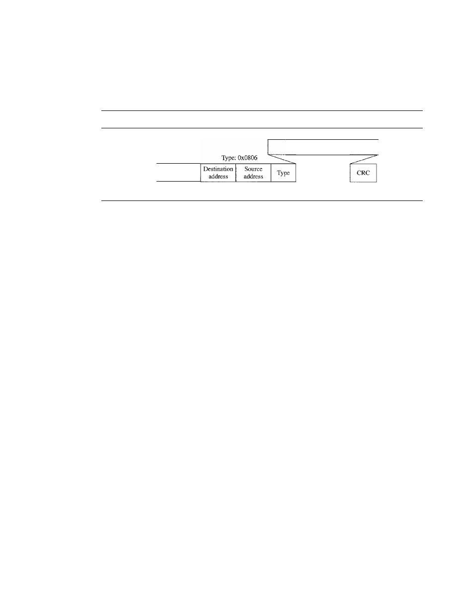
SECTION
21.1
ADDRESS MAPPING
615
Encapsulation
An
ARP packet is encapsulated directly into a data link frame. For example, in Figure 21.3
an ARP packet is encapsulated in an Ethernet frame. Note that the type field indicates that
the data carried by the frame are an ARP packet.
Figure 21.3
Encapsulation ofARP packet
ARP request or reply packet
Preamble
and SPD
8 bytes
6 bytes
6 bytes
2 bytes
Data
4 bytes
Operation
Let us see how ARP functions on a typical internet. First we describe the steps involved.
Then we discuss the four cases in which a host or router needs to use ARP. These are the
steps involved in an ARP process:
1. The sender knows the IP address of the target. We will see how the sender obtains
this shortly.
2. IP asks ARP to create an ARP request message, filling in the sender physical address,
the sender IP address, and the target IP address. The target physical address field is
filled with Os.
3. The message is passed to the data link layer where it is encapsulated in a frame by
using the physical address of the sender as the source address and the physical
broadcast address as the destination address.
4. Every host or router receives the frame. Because the frame contains a broadcast
destination address, all stations remove the message and pass it to ARP. All
machines except the one targeted drop the packet. The target machine recognizes
its IP address.
5. The target machine replies with an ARP reply message that contains its physical
address. The message is unicast.
6. The sender receives the reply message.
It
now knows the physical address of the
target machine.
7. The IP datagram, which carries data for the target machine, is now encapsulated in
a frame and is unicast to the destination.
Four Different Cases
The following are four different cases in which the services of ARP can be used (see
Figure 21.4).
1. The sender is a host and wants to send a packet to another host on the same net-
work. In this case, the logical address that must be mapped to a physical address is
the destination IP address in the datagram header.
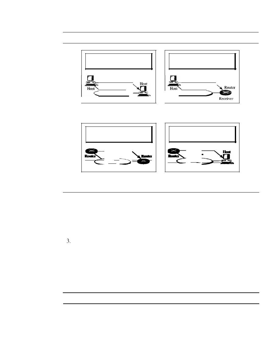
616
CHAPTER
21
NETWORK LAYER: ADDRESS MAPPING, ERROR REPORTING, AND MULTICASTING
Figure 21.4
Four cases using ARP
Target IP address:
Destination address in the IP datagram
Sender
LAN
Receiver
Case
1.
A host has a packet to send to
another host on the same network.
Target IF address:
IF address of the appropriate router
found in the routing table
Sender
...
LAN
Receiver
Case 3. A router receives a packet to be sent
to a host on another network.
It
must first
be delivered to the appropriate router.
Target IP address:
IP address of a router
Sender
LAN
Case 2. A host wants to send a packet to
another host on another network.
It
must first be delivered to a router.
Target IP address:
Destination address in the IP datagram
Sender
..
LAN
Receiver
Case 4. A router receives a packet to be sent
to a host on the same network.
2. The sender is a host and wants to send a packet to another host on another network.
In this case, the host looks at its routing table and finds the IP address of the next
hop (router) for this destination.
If
it
does not have a routing table,
it
looks for the
IP address of the default router. The IP address of the router becomes the logical
address that must be mapped to a physical address.
The sender is a router that has received a datagram destined for a host on another
network.
It
checks its routing table and finds the IP address of the next router. The
IP address of the next router becomes the logical address that must be mapped to a
physical address.
4. The sender is a router that has received a datagram destined for a host on the same
network. The destination IP address of the datagram becomes the logical address
that must be mapped to a physical address.
An ARP request is broadcast; an ARP reply is unicast.
Example 21.1
A host with IP address 130.23.43.20 and physical address B2:34:55: 10:22: 10 has a packet to
send to another host with IP address 130.23.43.25 and physical address A4:6E:F4:59:83:AB
(which is unknown to the first host). The two hosts are on the same Ethernet network. Show the
ARP request and reply packets encapsulated in Ethernet frames.
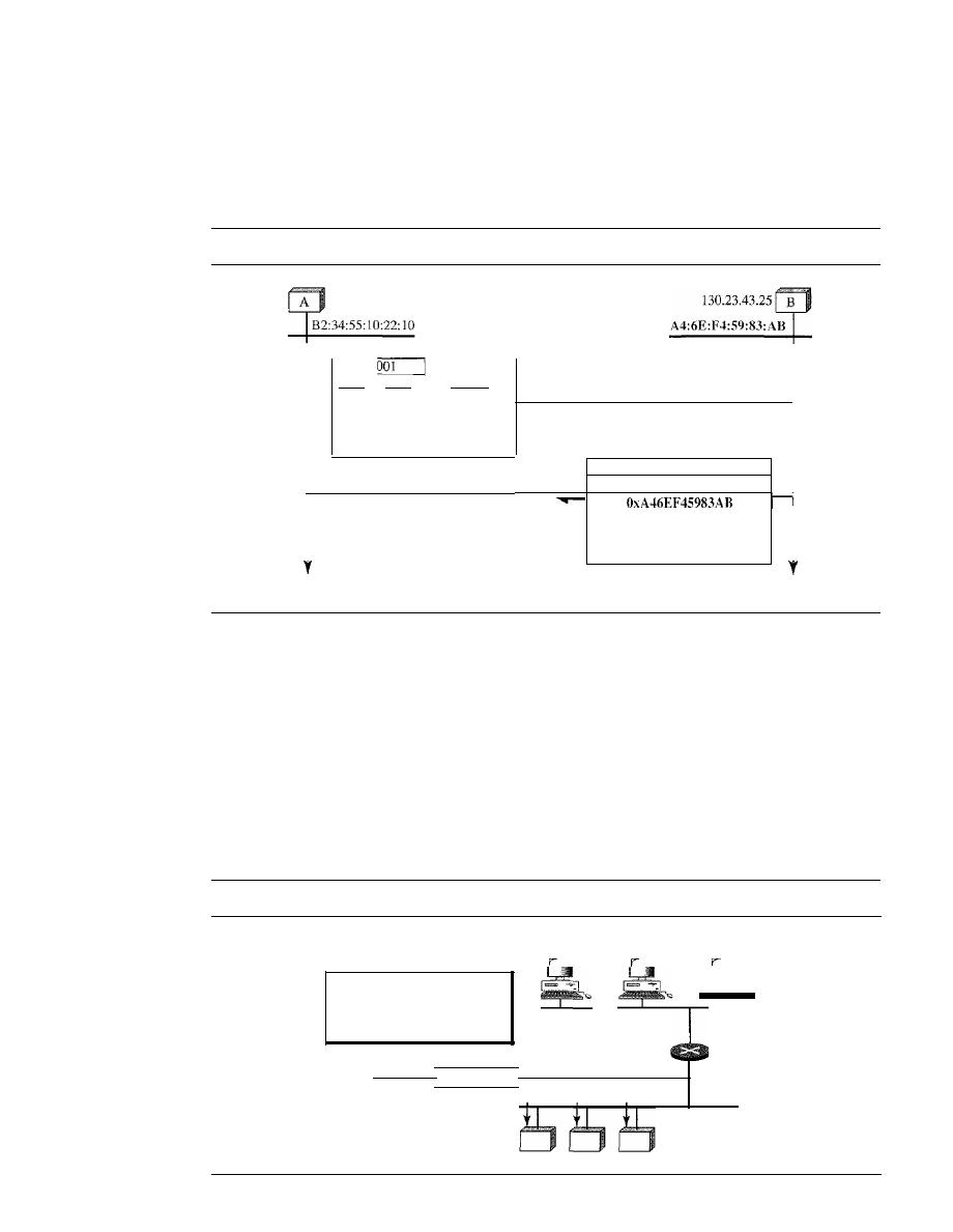
SECTION
21.1
ADDRESS MAPPlNG
617
Solution
Figure 21.5 shows the ARP request and reply packets. Note that the ARP data field in this case is
28 bytes, and that the individual addresses do not fit in the 4-byte boundary. That is why we do
not show the regular 4-byte boundaries for these addresses.
Figure
21.5
Example
21.1,
anARP request and reply
130.23.43.20
ARPRequest
OxOOOI
Ox0800
Ox06
Ox04
OxOOOl
OxB23455102210
130.23.43.20
OxOOOOOOOOOOOO
130.23.43.25
ARPReply
Time
OxOOOl
I
Ox0800
Ox06
I
Ox04
I
OxOO02
I
I
130.23.43.25
I
I
I
I
OxB2345510221O
I
I
130.23.43.20
I
I
I
Time
ProxyARP
A technique called proxy ARP is used to create a subnetting effect. A proxy ARP is an
ARP that acts on behalf of a set of hosts. Whenever a router running a proxy ARP
receives an ARP request looking for the IP address of one of these hosts, the router
sends an ARP reply announcing its own hardware (physical) address. After the router
receives the actual IP packet, it sends the packet to the appropriate host or router.
Let us give an example. In Figure 21.6 the ARP installed on the right-hand host
will answer only to anARP request with a target IP address of 141.23.56.23.
Figure
21.6
Proxy ARP
141.23.56.21
141.23.56.22
141.23.56.23
Added subnetwork
The proxy ARP router replies
to any ARP request received
for destinations 141.23.56.21,
141.23.56.22, and 141.23.56.23.
Proxy ARP
router
Request
Router or host

618
CHAPTER
21
NETWORK LAYER: ADDRESS MAPPING, ERROR REPORTING, AND MULTICASTING
However, the administrator may need to create a subnet without changing the
whole system to recognize subnetted addresses. One solution is to add a router running
a proxy ARP. In this case, the router acts on behalf of all the hosts installed on the subnet.
When it receives an ARP request with a target IP address that matches the address
of one of its
(141.23.56.21, 141.23.56.22, or 141.23.56.23), it sends an ARP
reply and announces its hardware address as the target hardware address. When the
router receives the IP packet, it sends the packet to the appropriate host.
Mapping Physical to Logical Address: RARP, BOOTP, and DHCP
There are occasions in which a host knows its physical address, but needs to know its
logical address. This may happen in two cases:
1. A diskless station is just booted. The station can find its physical address by checking
its interface, but it does not know its IP address.
2. An organization does not have enough IP addresses to assign to each station; it needs
to assign IP addresses on demand. The station can send its physical address and
ask for a short time lease.
RARP
Reverse Address Resolution Protocol
(RARP) finds the logical address for a machine
that knows only its physical address. Each host or router is assigned one or more logical
(IP) addresses, which are unique and independent of the physical (hardware) address of
the machine. To create an IP datagram, a host or a router needs to know its own IP
address or addresses. The IP address of a machine is usually read from its configuration
file stored on a disk file.
However, a diskless machine is usually booted from ROM, which has minimum
booting information. The ROM is installed by the manufacturer.
It
cannot include
the IP address because the IP addresses on a network are assigned by the network
administrator.
The machine can get its physical address (by reading its NIC, for example), which
is unique locally. It can then use the physical address to get the logical address by using
the RARP protocol. A RARP request is created and broadcast on the local network.
Another machine on the local network that knows all the IP addresses will respond with
a RARP reply. The requesting machine must be running a RARP client program; the
responding machine must be running a RARP server program.
There is a serious problem with RARP: Broadcasting is done at the data link layer. The
physical broadcast address, allis in the case of Ethernet, does not pass the boundaries of
a network. This means that if an administrator has several networks or several subnets, it
needs to assign a RARP server for each network or subnet. This is the reason that RARP
is almost obsolete.
protocols, BOOTP and DHCp, are replacing RARP.
BOOTP
The
Bootstrap Protocol (BOOTP)
is a client/server protocol designed to provide
physical address to logical address mapping. BOOTP is an application layer protocol.
The administrator may put the client and the server on the same network or on different
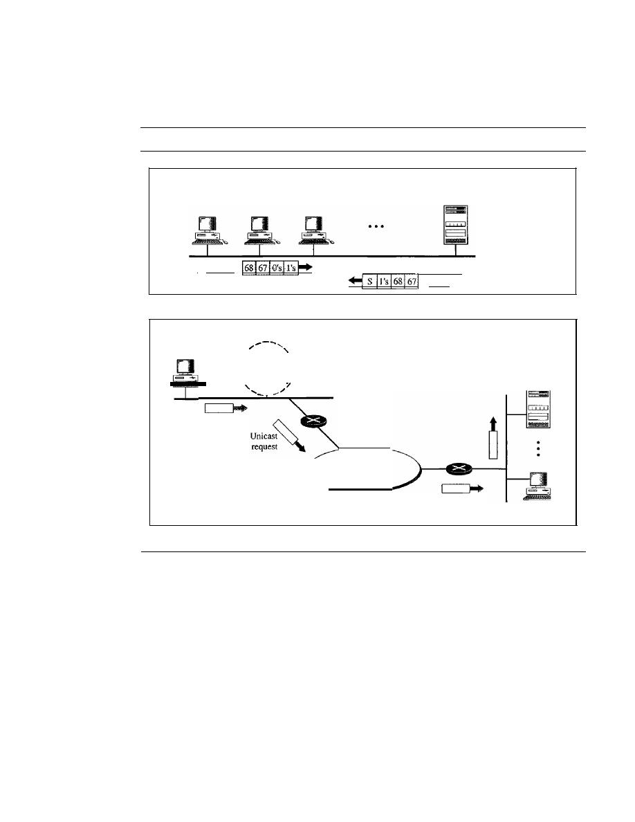
SECTION
21.1
ADDRESS MAPPING
619
networks, as shown in Figure 21.7. BOOTP messages are encapsulated in a UDP packet,
and the UDP packet itself is encapsulated in an IP packet.
Figure 21.7
BOOTP client and server on the same and different network
D
BOOTP
Client
BOOTPD
Server
I
Request
Reply
a. Client and server on the same network
Broadcast
request
server
D
BOOTP
Unicast
request
Internet
Relay agent
I
I
\
,
\
\
I
\
I
D
BOOTP
Client
b. Client and server on different networks
The reader may ask how a client can send an IP datagram when it knows neither
its own IP address (the source address) nor the server's IP address (the destination
address). The client simply uses all as as the source address and allIs as the destination
address.
One of the advantages of BOOTP over RARP is that the client and server are
application-layer processes. As in other application-layer processes, a client can be in
one network and the server in another, separated by several other networks. However,
there is one problem that must be solved. The BOOTP request is broadcast because the
client does not know the IP address of the server. A broadcast IP datagram cannot pass
through any router. To solve the problem, there is a need for an intermediary. One of the
hosts (or a router that can be configured to operate at the application layer) can be used
as a relay. The host in this case is called a relay agent. The relay agent knows the unicast
address of a BOOTP server. When it receives this type of packet, it encapsulates the
message in a unicast datagram and sends the request to the BOOTP server. The packet,

620
CHAPTER
21
NETWORK LAYER: ADDRESS MAPPING, ERROR REPORTING, AND MULTICASTING
carrying a unicast destination address, is routed by any router and reaches the BOOTP
server. The BOOTP server knows the message comes from a relay agent because one of
the fields in the request message defines the IP address of the relay agent. The relay
agent, after receiving the reply, sends it to the BOOTP client.
DHCP
BOOTP is not a dynamic configuration protocol. When a client requests its IP
address, the BOOTP server consults a table that matches the physical address of the client
with its IP address. This implies that the binding between the physical address and the
IP address of the client already exists. The binding is predetermined.
However, what if a host moves from one physical network to another? What if a
host wants a temporary IP address? BOOTP cannot handle these situations because the
binding between the physical and IP addresses is static and fixed in a table until changed
by the administrator. BOOTP is a static configuration protocol.
The Dynamic Host Configuration Protocol (DHCP) has been devised to provide
static and dynamic address allocation that can be manual or automatic.
DHCP provides static and dynamic address allocation that can be manual or automatic.
Static Address Allocation
In this capacity DHCP acts as BOOTP does. It is backward-
compatible with BOOTP, which means a host running the BOOTP client can request a
static address from a DHCP server. A DHCP server has a database that statically binds
physical addresses to IP addresses.
Dynamic Address Allocation
DHCP has a second database with a pool of available
IP addresses. This second database makes DHCP dynamic. When a DHCP client requests
a temporary IP address, the DHCP server goes to the pool of available (unused) IP
addresses and assigns an IP address for a negotiable period of time.
When a DHCP client sends a request to a DHCP server, the server first checks its
static database.
If
an entry with the requested physical address exists in the static data-
base, the permanent IP address of the client is returned. On the other hand, if the entry
does not exist in the static database, the server selects an IP address from the available
pool, assigns the address to the client, and adds the entry to the dynamic database.
The dynamic aspect of DHCP is needed when a host moves from network to net-
work or is connected and disconnected from a network (as is a subscriber to a service
provider). DHCP provides temporary IP addresses for a limited time.
The addresses assigned from the pool are temporary addresses. The DHCP server
issues a lease for a specific time. When the lease expires, the client must either stop
using the IP address or renew the lease. The server has the option to agree or disagree
with the renewal. If the server disagrees, the client stops using the address.
Manual and Automatic Configuration
One major problem with the BOOTP protocol
is that the table mapping the IP addresses to physical addresses needs to be manually
configured. This means that every time there is a change in a physical or IP address, the
administrator needs to manually enter the changes. DHCP, on the other hand, allows
both manual and automatic configurations. Static addresses are created
dynamic
addresses are created automatically.

SECTION
21.2
ICMP
621
21.2
ICMP
As discussed in Chapter 20, the IP provides unreliable and connectionless datagram
delivery.
It
was designed this way to make efficient use of network resources. The IP
protocol is a best-effort delivery service that delivers a datagram from its original
source to its final destination. However, it has two deficiencies: lack of error control and
lack of assistance mechanisms.
The IP protocol has no error-reporting or error-correcting mechanism. What happens
if something goes wrong? What happens if a router must discard a datagram because it
cannot find a router to the final destination, or because the time-to-live field has a zero
value? What happens if the final destination host must discard all fragments of a datagram
because it has not received all fragments within a predetermined time limit? These are
examples of situations where an error has occurred and the IP protocol has no built-in
mechanism to notify the original host.
The IP protocol also lacks a mechanism for host and management queries. A host
sometimes needs to determine if a router or another host is alive. And sometimes a net-
work administrator needs information from another host or router.
The
Internet Control Message Protocol (ICMP)
has been designed to compensate
for the above two deficiencies.
It
is a companion to the IP protoco1.
Types of Messages
ICMP messages are divided into two broad categories:
error-reporting messages
and
query messages.
The error-reporting messages report problems that a router or a host (destination)
may encounter when
it
processes an IP packet.
The query messages, which occur in pairs, help a host or a network manager get
specific information from a router or another host. For example, nodes can discover
their neighbors. Also, hosts can discover and learn about routers on their network, and
routers can help a node redirect its messages.
Message Format
An ICMP message has an 8-byte header and a variable-size data section. Although the
general format of the header is different for each message type, the first 4 bytes are com-
mon to all. As Figure 21.8 shows, the first field, ICMP type, defines the type of the
Figure 21.8
Generalformat of [CM? messages
8 bits
8 bits
8 bits
8 bits
Type
I
Code
I
Checksum
Rest of the header
Data section
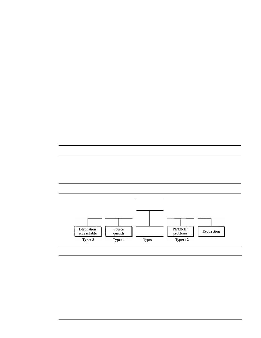
622
CHAPTER
21
NETWORK LAYER: ADDRESS MAPPING, ERROR REPORTING, AND MULTICASTING
message. The code field specifies the reason for the particular message type. The last
common field is the checksum field (to be discussed later in the chapter). The rest of the
header is specific for each message type.
The data section in error messages carries information for finding the original
packet that had the error.
In
query messages, the data section carries extra information
based on the type of the query.
Error Reporting
One of the main responsibilities of ICMP is to report errors. Although technology has
produced increasingly reliable transmission media, errors still exist and must be handled.
IP, as discussed in Chapter 20, is an unreliable protocol. This means that error checking
and error control are not a concern of IP. ICMP was designed, in part, to compensate for
this shortcoming. However, ICMP does not correct errors-it simply reports them. Error
correction is left to the higher-level protocols. Error messages are always sent to the orig-
inal source because the only information available in the datagram about the route is the
source and destination IP addresses. ICMP uses the source IP address to send the error
message to the source (originator) of the datagram.
ICMP always reports error messages to the original source.
Five types of errors are handled: destination unreachable, source quench, time
exceeded, parameter problems, and redirection (see Figure 21.9).
Figure 21.9
Error-reporting messages
Error
reporting
Time
exceeded
11
Type: 5
The following are important points about ICMP error messages:
o
No ICMP error message will be generated in response to a datagram carrying an
ICMP error message.
D
No ICMP error message will be generated for a fragmented datagram that is not
the first fragment.
D
No IeMP error message will be generated for a datagram having a multicast
address.
D
No ICMP error message will be generated for a datagram having a special address
such as 127.0.0.0 or 0.0.0.0.
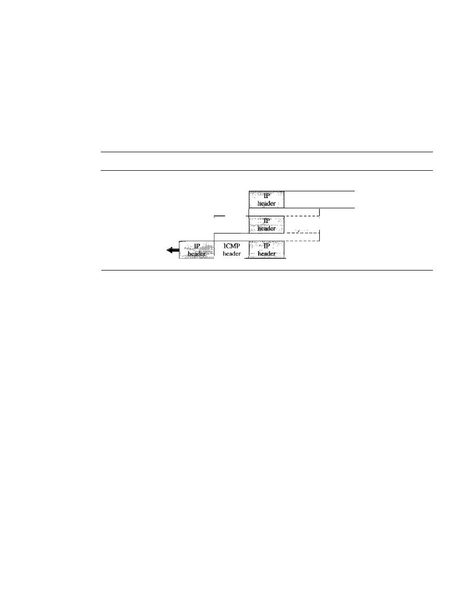
SECTION
21.2
ICMP
623
Note that all error messages contain a data section that includes the IP header of the
original datagram plus the first 8 bytes of data in that datagram. The original datagram
header is added to give the original source, which receives the error message, informa-
tion about the datagram itself. The 8 bytes of data are included because, as we will see
in Chapter 23 on UDP and TCP protocols, the first 8 bytes provide information about
the port numbers (UDP and TCP) and sequence number (TCP). This information is
needed so the source can inform the protocols (TCP or UDP) about the error. ICMP
forms an error packet, which is then encapsulated in an IP datagram (see Figure 21.10).
Figure
21.10
Contents of data field for the error messages
8
:
Rest
of
bytes
I
IP data
Received datagram
ICMP
header
8
I
bytes
:ICMP packet
8
I
bytes
: Sent IP datagram
___
J
Destination Unreachable
When a router cannot route a datagram or a host cannot deliver a datagram, the datagram
is discarded and the router or the host sends a destination-unreachable message back to
the source host that initiated the datagram. Note that destination-unreachable messages
can be created by either a router or the destination host.
Source Quench
The IP protocol is a connectionless protocol. There is no communication between the
source host, which produces the datagram, the routers, which forward it, and the destina-
tion host, which processes it. One of the ramifications of this absence of communication
is the lack of flow control. IP does not have a flow control mechanism embedded in the
protocol. The lack of flow control can create a major problem in the operation of IP:
congestion. The source host never knows if the routers or the destination host has been
overwhelmed with datagrams. The source host never knows if it is producing datagrams
faster than can be forwarded by routers or processed by the destination host.
The lack of flow control can create congestion in routers or the destination host.
A router or a host has a limited-size queue (buffer) for incoming datagrams waiting to
be forwarded (in the case of a router) or to be processed (in the case of a host).
If
the
datagrams are received much faster than they can be forwarded or processed, the
queue may overflow. In this case, the router or the host has no choice but to discard
some of the datagrams. The source-quench message in ICMP was designed to add a
kind of flow control to the IP. When a router or host discards a datagram due to con-
gestion, it sends a source-quench message to the sender of the datagram. This message
has two purposes. First, it informs the source that the datagram has been discarded.
Second, it warns the source that there is congestion somewhere in the path and that the
source should slow down (quench) the sending process.
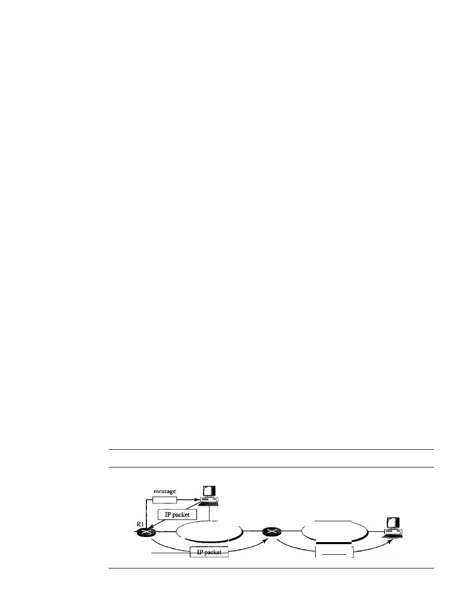
624
CHAPTER
21
NETWORK LAYER: ADDRESS MAPPING, ERROR REPORTING, AND MULTICASTING
Time Exceeded
The time-exceeded message is generated in two cases: As we see in Chapter 22, routers
use routing tables to find the next hop (next router) that must receive the packet.
If
there
are errors in one or more routing tables, a packet can travel in a loop or a cycle, going
from one router to the next or visiting a series of routers endlessly. As we saw in Chap-
ter 20, each datagram contains a field called
time to live
that controls this situation.
When a datagram visits a router, the value of this field is decremented by 1. When the
time-to-live value reaches 0, after decrementing, the router discards the datagram. How-
ever, when the datagram is discarded, a time-exceeded message must be sent by the
router to the original source. Second, a time-exceeded message is also generated when
not all fragments that make up a message arrive at the destination host within a certain
time limit.
Parameter Problem
Any ambiguity in the header part of a datagram can Create serious problems as the data-
gram travels through the Internet.
If
a router or the destination host discovers an ambig-
uous or missing value in any field of the datagram, it discards the datagram and sends a
parameter-problem message back to the source.
Redirection
When a router needs to send a packet destined for another network, it must know the IP
address of the next appropriate router. The same is true if the sender is a host. Both routers
and hosts, then, must have a routing table to find the address of the router or the next
router. Routers take part in the routing update process, as we will see in Chapter 22, and
are supposed to be updated constantly. Routing is dynamic.
However, for efficiency, hosts do not take part in the routing update process because
there are many more hosts in an internet than routerS. Updating the routing tables of hosts
dynamically produces unacceptable traffic. The hosts usually use static routing. When a
host comes up, its routing table has a limited number of entries. It usually knows the IP
address of only one router, the default router. For this reason, the host may send a data-
gram, which is destined for another network, to the wrong router. In this case, the router
that receives the datagram will forward the datagram to the correct router. However, to
update the routing table of the host, it sends a redirection message to the host. This con-
cept of redirection is shown in Figure 21.11. Host A wants to send a datagram to host
B.
Figure
21.11
Redirection concept
Redirection
A
LAN
R2
LAN
lPpacket
B
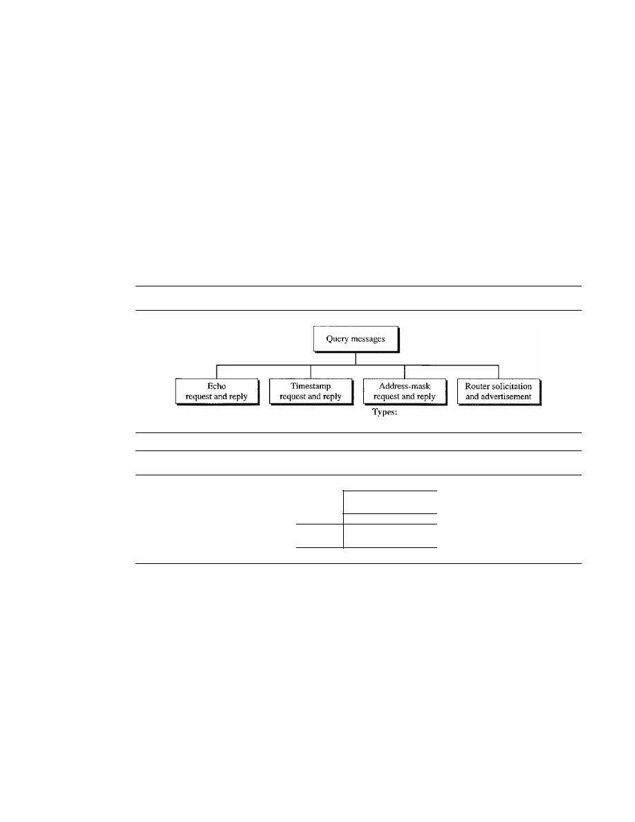
SECTION
21.2
ICMP
625
Router R2 is obviously the most efficient routing choice, but host A did not choose
router R2. The datagram goes to R1 instead. Router R1, after consulting its table, finds
that the packet should have gone to R2. It sends the packet to R2 and, at the same time,
sends a redirection message to host
A.
Host A's routing table can now be updated.
Query
In addition to error reporting, ICMP can diagnose some network problems. This is
accomplished through the query messages, a group of four different pairs of messages,
as shown in Figure 21.12. In this type of ICMP message, a node sends a message that
is answered in a specific format by the destination node. A query message is encapsu-
lated in an IP packet, which in tum is encapsulated in a data link layer frame. However, in
this case, no bytes of the original IP are included in the message, as shown in Figure 21.13.
Figure
21.12
Query messages
Types: 8 and 0
Types: 13 and 14
17 and 18
Types: 10 and 9
Figure
21.13
Encapsulation of ICMP query messages
IeMP
Packet
IP
IP
header
Data
Echo Request and Reply
The echo-request and echo-reply messages are designed for diagnostic purposes. Net-
work managers and users utilize this pair of messages to identify network problems. The
combination of echo-request and echo-reply messages detennines whether two systems
(hosts or routers) can communicate with each other. The echo-request and echo-reply
messages can be used to determine if there is communication at the IP level. Because
ICMP messages are encapsulated in IP datagrams, the receipt of an echo-reply message
by the machine that sent the echo request is proof that the IP protocols in the sender and
receiver are communicating with each other using the IP datagram. Also, it is proof that
the intermediate routers are receiving, processing, and forwarding IP datagrams. Today,
most systems provide a version of the
ping
command that can create a series (instead of
just one) of echo-request and echo-reply messages, providing statistical information. We
will see the use of this program at the end of the chapter.
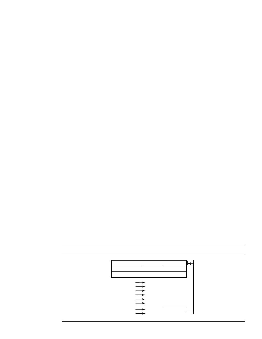
626
CHAPTER 21
NETWORK lAYER: ADDRESS MAPPING, ERROR REPORTING, AND MULTICASTING
Timestamp Request and Reply
Two machines (hosts or routers) can use the
timestamp request and timestamp reply
messages
to determine the round-trip time needed for an IP datagram to travel between
them.
It
can also be used to synchronize the clocks in two machines.
Address-Mask Request and Reply
A host may know its IP address, but it may not know the corresponding mask. For
example, a host may know its IP address as 159.31.17.24, but it may not know that the
corresponding mask is /24. To obtain its mask, a host sends an
address-mask-request
message
to a router on the LAN.
If
the host knows the address of the router, it sends the
request directly to the router.
If
it does not know,
it
broadcasts the message. The router
receiving the address-mask-request message responds with an
address-mask-reply
message,
providing the necessary mask for the host. This can be applied to its full IP
address to get its subnet address.
Router Solicitation and Advertisement
As we discussed in the redirection message section, a host that wants to send data to a host
on another network needs to know the address of routers connected to its own network.
Also, the host must know if the routers are alive and functioning. The
router-solicitation
and router-advertisement messages
can help in this situation. A host can broadcast (or
multicast) a router-solicitation message. The router or routers that receive the solicitation
message broadcast their routing information using the router-advertisement message. A
router can also periodically send router-advertisement messages even if no host has solic-
ited. Note that when a router sends out an advertisement, it announces not only its own
presence but also the presence of all routers on the network of which it is aware.
Checksum
In Chapter 10, we learned the concept and idea of the checksum. In ICMP the checksum
is calculated over the entire message (header and data).
Example 21.2
Figure 21.14 shows an example of checksum calculation for a simple echo-request message. We
randomly chose the identifier to be 1 and the sequence number to be 9. The message is divided
Figure 21.14
Example of checksum calculation
Checksum
111010000 0 0
100
8
I
0
\
0
I
I
9
TEST
8 & 0
00001000 00000000
o
00000000 00000000
1
00000000 00000001
9
00000000 00001001
T&E
01010100 01000101
S & T
01010011 01010100
Sum
10101111
10100011
1 11

SECTION
21.2
ICMP
627
into 16-bit (2-byte) words. The words are added and the sum is complemented. Now the sender
can put this value in the checksum field.
Debugging Tools
There are several tools that can be used in the Internet for debugging. We can determine
the viability of a host or router. We can trace the route of a packet. We introduce two
tools that use ICMP for debugging: ping and traceroute. We will introduce more tools
in future chapters after we have discussed the corresponding protocols.
Ping
We can use the ping program to find if a host is alive and responding. We use ping here
to see how it uses ICMP packets.
The source host sends ICMP echo-request messages (type: 8, code: 0); the destina-
tion, if alive, responds with ICMP echo-reply messages. The ping program sets the identi-
fier field in the echo-request and echo-reply message and stans the sequence number
from 0; this number is incremented by 1 each time a new message is sent. Note that ping
can calculate the round-trip time.
It
inserts the sending time in the data section of the
message. When the packet arrives, it subtracts the arrival time from the departure time to
get the round-trip time (RTT).
Example 21.3
We use the
ping
program to test the server fhda.edu. The result is shown below:
$ ping thda.edu
PING thda.edu (153.18.8.1)
56 (84) bytes of data.
64 bytes from tiptoe.fhda.edu (153.18.8.1): icmp_seq=O
64 bytes from tiptoe.fhda.edu (153.18.8.1): icmp_seq=l
64 bytes from tiptoe.fhda.edu (153.18.8.1): icmp_seq=2
64 bytes from tiptoe.fhda.edu (153.18.8.1): icmp_seq=3
64 bytes from tiptoe.fhda.edu (153.18.8.1): icmp_seq=4
64 bytes from tiptoe.fhda.edu (153.18.8.1): icmp_seq=5
64 bytes from tiptoe.fhda.edu (153.18.8.1): icmp_seq=6
64 bytes from tiptoe.:fhda.edu (153.18.8.1): icmp_seq=7
64 bytes from tiptoe.:fhda.edu (153.18.8.1): icmp_seq=8
64 bytes from tiptoe.fhda.edu (153.18.8.1): icmp_seq=9
64 bytes from tiptoe.:fhda.edu (153.18.8.1): icmp_seq=lO
ttl=62
ttl=62
ttl=62
ttl=62
ttl=62
ttl=62
tt1=62
ttl=62
ttl=62
ttl=62
ttl==62
time=1.91 ms
ms
time=1.90 ms
time=1.97 ms
time=1.93 ms
time=2.00 ms
time=1.94 ms
time=1.94 ms
time=1.97 ms
time=1.89 ms
time=1.98 ms
--- thda.edu ping statistics ---
11 packets transmitted, 11 received, 0% packet loss, time 10103ms
rtt minJavg/max = 1.899/1.955/2.041 ms
The
ping
program sends messages with sequence numbers starting from O. For each probe it
gives us the RTT time. The TTL (time to live) field in the IP datagram that encapsulates an ICMP
message has been set to 62, which means the packet cannot travel mare than 62 hops. At the begin-
ning,
ping
defines the number of data bytes as 56 and the total number of bytes as 84. It is obvious
that if we add 8 bytes of ICMP header and 20 bytes of IP header to 56, the result is 84. However,
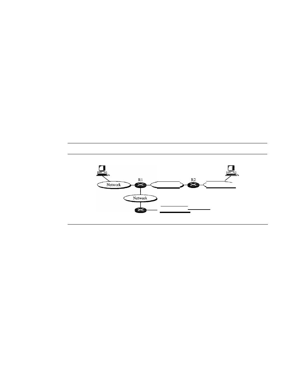
628
CHAPTER 21
NETWORK IAYER: ADDRESS MAPPING, ERROR REPORTiNG, AND MULTiCASTING
note that in each probe
ping
defines the number of bytes as 64. This is the total number of bytes in
the ICMP packet (56
+
8). The
ping
program continues to send messages, if we do not stop it by
using the interrupt key (ctrl
+
c, for example). After it is interrupted, it prints the statistics of the
probes.
It
tells us the number of packets sent, the number of packets received, the total time, and
the RTT minimum, maximum, and average. Some systems may print more infonnation.
Tracerollte
The
traceroute
program in UNIX or
tracert
in Windows can be used to trace the route
of a packet from the source to the destination. We have seen an application of the
traceroute
program to simulate the loose source route and strict source route options of
an IP datagram in Chapter 20. We use this program in conjunction with ICMP packets
in this chapter. The program elegantly uses two ICMP messages, time exceeded and
destination unreachable, to find the route of a packet. This is a program at the applica-
tion level that uses the services of UDP (see Chapter 23). Let us show the idea of the
traceroute
program by using Figure 21.15.
Figure 21.15
The traceroute program operation
Host A
Network
Network
R3
Hoste
HostB
Network
Given the topology, we know that a packet from host A to host B travels through
routers Rl and R2. However, most of the time, we are not aware of this topology. There
could be several routes from A to
B.
The traceroute program uses the ICMP messages
and the TTL (time to live) field in the IP packet to find the route.
1.
The traceroute program uses the following steps to find the address of the router Rl
and the round-trip time between host A and router Rl.
a. The traceroute application at host A sends a packet to destination Busing UDP;
the message is encapsulated in an IP packet with a TTL value of 1. The program
notes the time the packet is sent.
b. Router Rl receives the packet and decrements the value of TTL to O. It then dis-
cards the packet (because TTL is 0). The router, however, sends a time-exceeded
ICMP message (type: 11, code: 0) to show that the TTL value is 0 and the packet
was discarded.
c. The trace route program receives the ICMP messages and uses the destination
address of the IP packet encapsulating ICMP to find the IP address of router Rl.
The program also makes note of the time the packet has arrived. The difference
between this time and the time at step a is the round-trip time.

SECTION
21.2
ICMP
629
The traceroute program repeats steps a to c three times to get a better average
round-trip time. The first trip time may be much longer than the second or third
because it takes time for the ARP program to find the physical address of router
RI. For the second and third trips, ARP has the address in its cache.
2. The traceroute program repeats the previous steps to find the address of router R2
and the round-trip time between host A and router R2. However, in this step, the
value of TTL is set to 2. So router RI forwards the message, while router R2 dis-
cards it and sends a time-exceeded ICMP message.
3. The traceroute program repeats step 2 to find the address of host B and the round-trip
time between host A and host B. When host B receives the packet,
it
decrements the
value of TIL, but it does not discard the message since it has reached its final desti-
nation. How can an ICMP message be sent back to host A? The traceroute program
uses a different strategy here. The destination port of the UDP packet is set to one
that is not supported by the UDP protocol. When host B receives the packet, it cannot
find an application program to accept the delivery.
It
discards the packet and sends an
ICMP destination-unreachable message (type: 3, code: 3) to host A. Note that this
situation does not happen at router RI or R2 because a router does not check the
UDP header. The traceroute program records the destination address of the arrived
IP datagram and makes note of the round-trip time. Receiving the destination-
unreachable message with a code value 3 is an indication that the whole route has
been found and there is no need to send more packets.
Example 21.4
We use the traceroute program to find the route from the computer voyager.deanza.edu to the
server fhda.edu. The following shows the result:
$
traceroute fbda.edu
traceroute to fbda.edu
1 Dcore.fhda.edu
2
Dbackup.fhda.edu
3 tiptoe.fhda.edu
(153.18.8.1),30
max, 38 byte packets
(153.18.31.254)
0.995 ms
0.899 ms
(153.18.251.4)
1.039
fiS
1.064
fiS
(153.18.8.1)
1.797
illS
1.642 ms
0.878 ms
1.083
fiS
1.757
fiS
The unnumbered line after the command shows that the destination is 153.18.8.1. The TIL
value is 30 hops. The packet contains 38 bytes: 20 bytes of IP header, 8 bytes of UDP header, and
10 bytes of application data. The application data are used by traceroute to keep track of the
packets.
The first line shows the first router visited. The router is named Dcore.fhda.edu with IP
address 153.18.31.254. The first round-trip time was 0.995 ms, the second was 0.899 ms, and the
third was 0.878 ms.
The second line shows the second router visited. The router is named Dbackup.fhda.edu
with IP address 153.18.251.4. The three round-trip times are also shown.
The third line shows the destination host. We know that this is the destination host because
there are no more lines. The destination host is the server thda.edu, but it is named tiptoe.fhda.edu
with the IP address 153.18.8.1. The three round-trip times are also shown.
Example 21.5
In this example, we trace a longer route, the route to xerox.com.

630
CHAPTER
21
NETWORK LAYER: ADDRESS MAPPING, ERROR REPORTING, AND MULTICASTING
$
traceroute xerox.com
traceroute to xerox.com (13.1.64.93), 30 hops max, 38 byte packets
1 Dcore.fbda.edu
(153.18.31.254)
0.622 ms
0.891 ms
2 Ddmz.fbda.edu
(153.18.251.40)
2.132 ms
2.266 ms
3 Cinic.fhda.edu
(153.18.253.126)
2.110 ms
2.145 ms
4 cenic.net
(137.164.32.140)
3.069 ms
2.875 ms
5 cenic.net
(137.164.22.31)
4.205 ms
4.870 ms
0.875 ms
2.094ms
1.763 ms
2.930ms
4.197 ms
14 snfc21.pbi.net
(151.164.191.49)
7.656 ms
7.129 ms
6.866ms
15 sbcglobaLnet
(151.164.243.58)
7.844 ms
7.545 ms
7.353 ms
16 pacbell.net
(209.232.138.114)
9.857 ms
9.535 ms
9.603 ms
17 209.233.48.223
(209.233.48.223)
10.634ms
10.771 ms
10.592 ms
18 alpha.Xerox.COM
(13.1.64.93)
11.172 ms
11.048 ms
10.922ms
Here there are 17 hops between source and destination. Note that some round-trip times look
unusual. It could be that a router was too busy to process the packet immediately.
21.3
IGMP
The IP protocol can be involved in two types of communication: unicasting and multi-
casting. Unicasting is the communication between one sender and one receiver.
It
is a
one-to-one communication. However, some processes sometimes need to send the same
message to a large number of receivers simultaneously. This is called
multicasting,
which is a one-to-many communication. Multicasting has many applications. For exam-
ple, multiple stockbrokers can simultaneously be informed of changes in a stock price,
or travel agents can be informed of a plane cancellation. Some other applications include
distance learning and video-on-demand.
The
Internet Group Management Protocol (IGMP)
is one of the necessary, but
not sufficient (as we will see), protocols that is involved in multicasting. IGMP is a
companion to the IP protocol.
Group Management
For multicasting in the Internet we need routers that are able to route multicast packets.
The routing tables of these routers must be updated by using one of the multicasting
routing protocols that we discuss in Chapter 22.
IGMP is not a multicasting routing protocol; it is a protocol that manages
group
membership.
In any network, there are one or more multicast routers that distribute
multicast packets to hosts or other routers. The IGMP protocol gives the
multicast routers
information about the membership status of hosts (routers) connected to the network.
A multicast router may receive thousands of multicast packets every day for different
groups.
If
a router has no knowledge about the membership status of the hosts, it must
broadcast all these packets. This creates a lot of traffic and consumes bandwidth. A better
solution is to keep a list of groups in the network for which there is at least one loyal
member. IGMP helps the multicast router create and update this list.
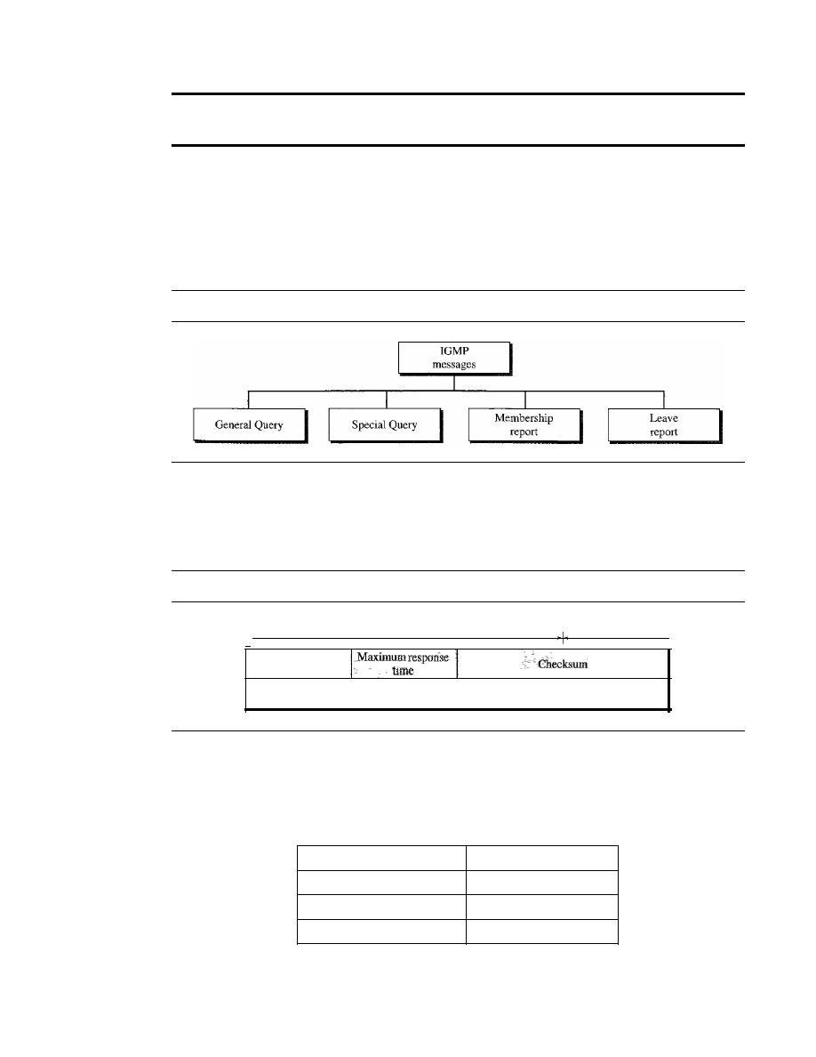
SECTION
21.3
IGMP
631
IGMP is a group management protocol.
It
helps a multicast router create
and update a list of loyal members related to each router interface.
IGMP Messages
IOMP has gone through two versions. We discuss IOMPv2, the current version. IOMPv2
has three types of
messages:
the
query,
the
membership report,
and the
leave report.
There are two types of
query messages: general
and
special
(see Figure 21.16).
Figure 21.16
IGMP message types
Message Format
Figure 21.17 shows the format of an IOMP (version 2) message.
Figure 21.17
IGMP message fonnat
I·
8 bits
Type
8 bits
8
bits
8 bits
Group address in membership and leave reports and special query; alIOs in general query
o
Type.
This 8-bit field defines the type of message, as shown in Table 21.1. The value
of the type is shown in both hexadecimal and binary notation.
Table 21.1
IGMP type field
Type
Value
General or special query
Ox 11
or
00010001
Membership report
Ox16
or
00010110
Leave report
Ox17
or
00010111
o
Maximum Response Time.
This 8-bit field defines the amount of time in which a
query must be answered. The value is in tenths of a second; for example, if the
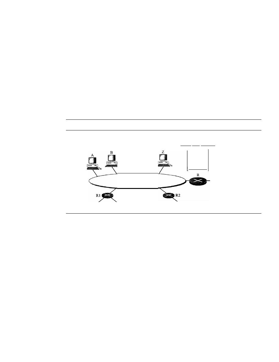
632
CHAPTER
21
NETWORK LAYER: ADDRESS MAPPING, ERROR REPORTING, AND MULTICASTING
value is 100, it means 10 s. The value is nonzero in the query message; it is set to
zero in the other two message types. We will see its use shortly.
D
Checksum.
This is a 16-bit field carrying the checksum. The checksum is calculated
over the 8-byte message.
D
Group address.
The value of this field is 0 for a general query message. The value
defines the groupid (multicast address of the group) in the special query, the mem-
bership report, and the leave report messages.
IGMP Operation
IGMP operates locally.
A
multicast router connected to a network has a list of multicast
addresses of the groups with at least one loyal member in that network (see Figure 21.18).
Figure
21.18
IGMP
operation
To another network
229.60.12.8
...
Network
List of groups
having loyal members
225.70.8.20
231.24.60.9
To other networks
To another network
For each group, there is one router that has the duty of distributing the multicast
packets destined for that group. This means that if there are three multicast routers
connected to a network, their lists of
groupids
are mutually exclusive. For example, in
Figure 21.18 only router R distributes packets with the multicast address of225.70.8.20.
A host or multicast router can have membership in a group. When a host has member-
ship, it means that one of its processes (an application program) receives multicast packets
from some group. When a router has membership, it means that a network connected to
one of its other interfaces receives these multicast packets. We say that the host or the
router has an interest in the group. In both cases, the host and the router keep a list of
groupids and relay their interest to the distributing router.
For example, in Figure 21.18, router R is the distributing router. There are two
other multicast routers (R1 and R2) that, depending on the group list maintained by
router R, could be the recipients of router R in this network. Routers R
I
and R2 may be
distributors for some of these groups in other networks, but not on this network.
Joining a Group
A host or a router can join a group. A host maintains a list of processes that have member-
ship in a group. When a process wants to join a new group, it sends its request to the host.

SECTION
21.3
IGMP
633
The host adds the name of the process and the name of the requested group to its list. If
this is the first entry for this particular group, the host sends a membership report mes-
sage.
If
this is not the first entry, there is no need to send the membership report since the
host is already a member of the group; it already receives multicast packets for this group.
The protocol requires that the membership report be sent twice, one after the other
within a few moments. In this way, if the first one is lost or damaged, the second one
replaces it.
In IGMP, a membership report is sent twice, one after the other.
Leaving a Group
When a host sees that no process is interested in a specific group,
it
sends a leave report.
Similarly, when a router sees that none of the networks connected to its interfaces is
interested in a specific group, it sends a leave report about that group.
However, when a multicast router receives a leave report, it cannot immediately
purge that group from its list because the report comes from just one host or router;
there may be other hosts or routers that are still interested in that group. To make sure,
the router sends a special query message and inserts the groupid, or
multicast address,
related to the group. The router allows a specified time for any host or router to respond.
If, during this time, no interest (membership report) is received, the router assumes that
there are no loyal members in the network and purges the group from its list.
Monitoring Membership
A host or router can join a group by sending a membership report message. It can leave
a group by sending a leave report message. However, sending these two types of reports
is not enough. Consider the situation in which there is only one host interested in a
group, but the host is shut down or removed from the system. The multicast router will
never receive a leave report. How is this handled? The multicast router is responsible
for monitoring all the hosts or routers in a LAN to see if they want to continue their
membership in a group.
The router periodically (by default, every 125 s) sends a general query message. In
this message, the group address field is set to 0.0.0.0. This means the query for member-
ship continuation is for all groups in which a host is involved, not just one.
The general query message does not define a particular group.
The router expects an answer for each group in its group list; even new groups may
respond. The query message has a maximum response time of 10 s (the value of the
field is actually 100, but this is in tenths of a second). When a host or router receives the
general query message, it responds with a membership report if it is interested in a
group. However, if there is a common interest (two hosts, for example, are interested in
the same group), only one response is sent for that group to prevent unnecessary traffic.
This is called a delayed response. Note that the query message must be sent by only one
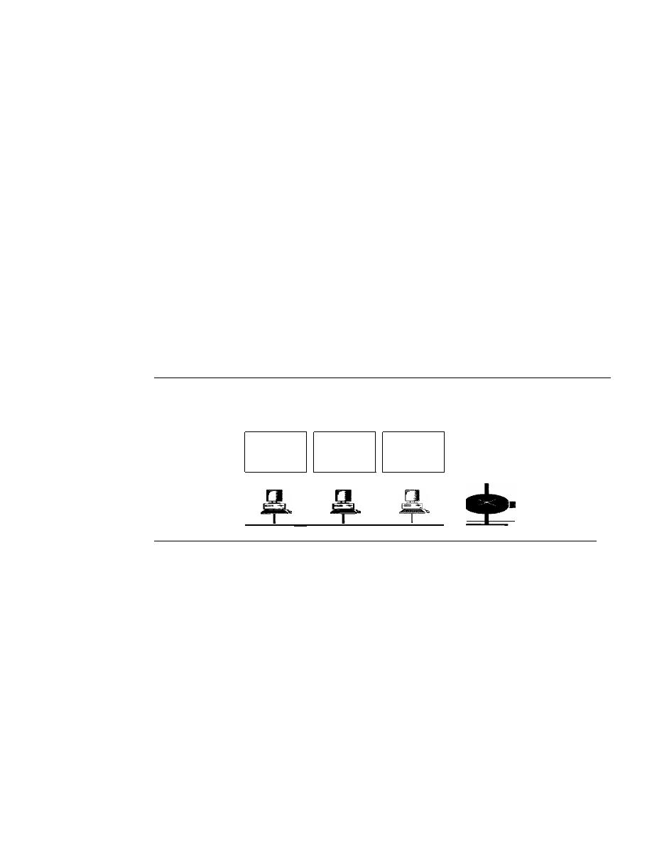
634
CHAPTER 21
NETWORK LAYER: ADDRESS MAPPING, ERROR REPORTING, AND MULTICASTING
router (normally called the query router), also to prevent unnecessary traffic. We discuss
this issue shortly.
Delayed Response
To prevent unnecessary traffic, IGMP uses a delayed response strategy. When a host or
router receives a query message, it does not respond immediately; it delays the response.
Each host or router uses a random number to create a timer, which expires between
I
and
lOs. The expiration time can be in steps of
I
s or less.
A
timer is set for each group in the
list. For example, the timer for the first group may expire in
2 s, but the timer for the third
group may expire in
5
s. Each host or router waits until its timer has expired before send-
ing a membership report message. During this waiting time, if the timer of another host or
router, for the same group, expires earlier, that host or router sends a membership report.
Because, as we will see shortly, the report is broadcast, the waiting host or router receives
the report and knows that there is no need to send a duplicate report for this group; thus,
the waiting station cancels its corresponding timer.
Example
21.6
Imagine there are three hosts in a network, as shown in Figure 21.19.
Figure 21.19
Example 21.6
Group
Timer
Group
Timer
Group
Timer
225.14.0.0
30
228.42.0.0
48
225.14.0.0 62
228.42.0.0
12
238.71.0.0
50
230.43.0.0 70
230.43.0.0
80
To other networks
A
B
C
A
query message was received at time 0; the random delay time (in tenths of seconds) for
each group is shown next to the group address. Show the sequence of report messages.
Solution
The events occur in this sequence:
a. Time
12:
The timer for 228.42.0.0 in host A expires, and a membership report is sent,
which is received by the router and every host including host
B
which cancels its timer
for 228.42.0.0.
b. Time 30: The timer for 225.14.0.0 in host A expires, and a membership report is sent,
which is received by the router and every host including host C which cancels its timer
for 225.14.0.0.
c. Time 50: The timer for 238.71.0.0 in host B expires, and a membership report is sent,
which is received by the router and every host.
d. Time
70:
The timer for 230.43.0.0 in host C expires, and a membership report is sent,
which is received by the router and every host including host A which cancels its timer
for 230.43.0.0.
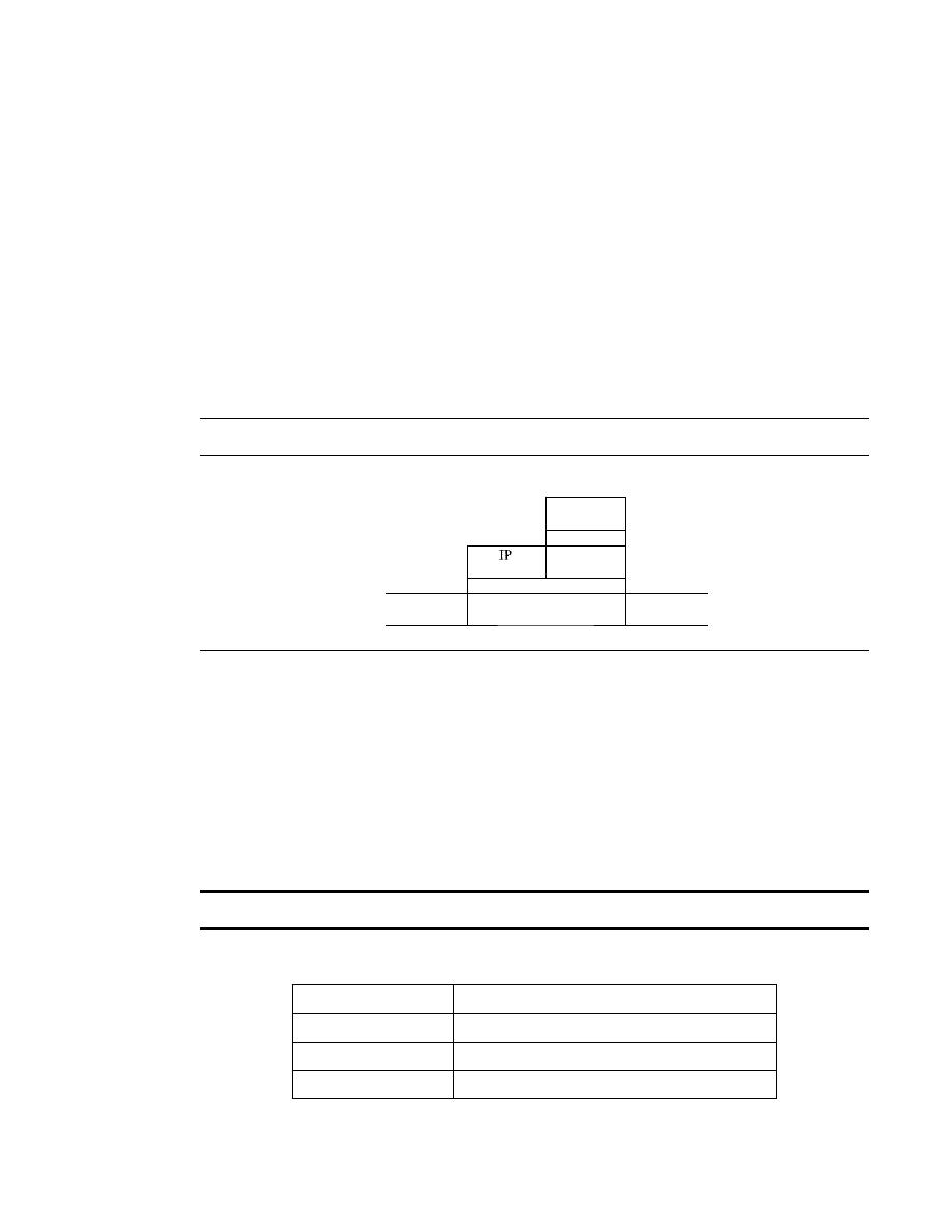
SECTION
21.3
IGMP
635
Note that if each host had sent a report for every group in its list, there would have been seven
reports; with this strategy only four reports are sent.
Query Router
Query messages may create a lot of responses. To prevent unnecessary traffic, IGMP
designates one router as the query router for each network. Only this designated router
sends the query message, and the other routers are passive (they receive responses and
update their lists).
Encapsulation
The IGMP message is encapsulated in an IP datagram, which is itself encapsulated in a
frame. See Figure 21.20.
Figure 21.20
Encapsulation ofIGMP packet
8 bytes
IGMP
message
IP
header
data
Frame
Frame
Trailer
I
header
data
(if
any)
Encapsulation at Network Layer
The value of the protocol field is 2 for the IGMP protocol. Every IP packet carrying this
value in its protocol field has data delivered to the IGMP protocol. When the message is
encapsulated in the IP datagram, the value of TTL must be
1.
This is required because
the domain of IGMP is the LAN. No IGMP message must travel beyond the LAN. A
TTL value of
1
guarantees that the message does not leave the LAN since this value is
decremented to 0 by the next router and, consequently, the packet is discarded. Table 21.2
shows the destination IP address for each type of message.
The IP packet that carries an IGMP packet has a value of 1 in its TTL field.
Table 21.2
Destination IP addresses
Type
IP Destination Address
Query
224.0.0.1 All systems on this subnet
Membership report
The multicast address of the group
Leave report
224.0.0.2 All routers on this subnet
A query message is multicast by using the multicast address 224.0.0.1 All hosts
and all routers will receive the message. A membership report is multicast using a
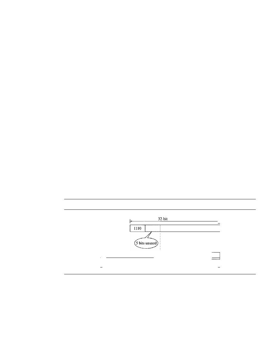
636
CHAPTER
21
NETWORK LAYER: ADDRESS MAPPING, ERROR REPORTING, AND MULTICASTING
destination address equal to the multicast address being reported (groupid). Every sta-
tion (host or router) that receives the packet can immediately determine (from the
header) the group for which a report has been sent. As discussed previously, the timers
for the corresponding unsent reports can then be canceled. Stations do not need to open
the packet to find the groupid. This address is duplicated in a packet; it's part of the
message itself and also a field in the IP header. The duplication prevents errors. A leave
report message is multicast using the multicast address
224.0.0.2 (all routers on this
subnet) so that routers receive this type of message. Hosts receive this message too, but
disregard it.
Encapsulation at Data Link Layer
At the network layer, the IGMP message is encapsulated in an IP packet and is treated
as an IP packet. However, because the IP packet has a multicast IP address, the ARP
protocol cannot find the corresponding MAC (physical) address to forward the packet
at the data link layer. What happens next depends on whether the underlying data link
layer supports physical multicast addresses.
Physical Multicast Support
Most LANs support physical multicast addressing. Ether-
net is one of them. An Ethernet physical address (MAC address) is six octets (48 bits)
long.
If
the first
25 bits in an Ethernet address are 0000000100000000010111100, this
identifies a physical multicast address for the TCP/IP protocol. The remaining 23 bits can
be used to define a group. To convert an IP multicast address into an Ethernet address, the
multicast router extracts the least significant 23 bits of a class D IP address and inserts
them into a multicast Ethernet physical address (see Figure
21.21).
Figure 21.21
Mapping class
D
to Ethernet physical address
-[
23 bits of multicast address
class D address
I
I
I
I
I
I
I
- - - - - - - - - - - - - - - - - - - - ,
1
0000000100000000010111100
2
__3__b__
its__o__
f __
ph__
y__
sic__
a__
la__
dd__re__s__
s
,-
48-bit Ethernet address
-I
However, the group identifier of a class D IP address is 28 bits long, which implies
that 5 bits is not used. This means that 32
(25)
multicast addresses at the IP level are
mapped to a single multicast address. In other words, the mapping is many-to-one
instead of one-to-one.
If
the 5 leftmost bits of the group identifier of a class D address
are not all zeros, a host may receive packets that do not really belong to the group in
which it is involved. For this reason, the host must check the IP address and discard any
packets that do not belong to it.
Other LANs support the same concept but have different methods of mapping.

SECTION
21.3
IGMP
637
An Ethernet multicast physical address is in the range
01 :00:5E:00:OO:OO
to
01:00:5E:7F:FF:FF.
Example 21.7
Change the multicast IP address 230.43.14.7 to an Ethernet multicast physical address.
Solution
We can do this in two steps:
a. We write the rightmost 23 bits of the IP address in hexadecimal. This can be done by changing
the rightmost 3 bytes to hexadecimal and then subtracting 8 from the leftmost digit if it is
greater than or equal to 8. In our example, the result is 2B:OE:07.
b. We add the result of part a to the starting Ethernet multicast address, which is
01:00:5E:00:00:00. The result is
01:00:5E:2B:OE:07
Example 21.8
Change the multicast IP address 238.212.24.9 to an Ethernet multicast address.
Solution
a. The rightmost 3 bytes in hexadecimal is D4: 18:09. We need to subtract 8 from the leftmost
digit, resulting in 54:18:09.
b. We add the result of part a to the Ethernet multicast starting address. The result is
01:00:5E:54: 18:09
No Physical Multicast Support
Most WANs do not support physical multicast address-
ing. To send a multicast packet through these networks, a process called
tunneling is used.
In
tunneling, the multicast packet is encapsulated in a unicast packet and sent through the
network, where it emerges from the other side as a multicast packet (see Figure 21.22).
Figure 21.22
Tunneling
Multicast IP datagram
Header
I
Data
Header
Data
Unicast IP datagram
Netstat
Utility
The
netstat utility can be used to find the multicast addresses supported by an interface.
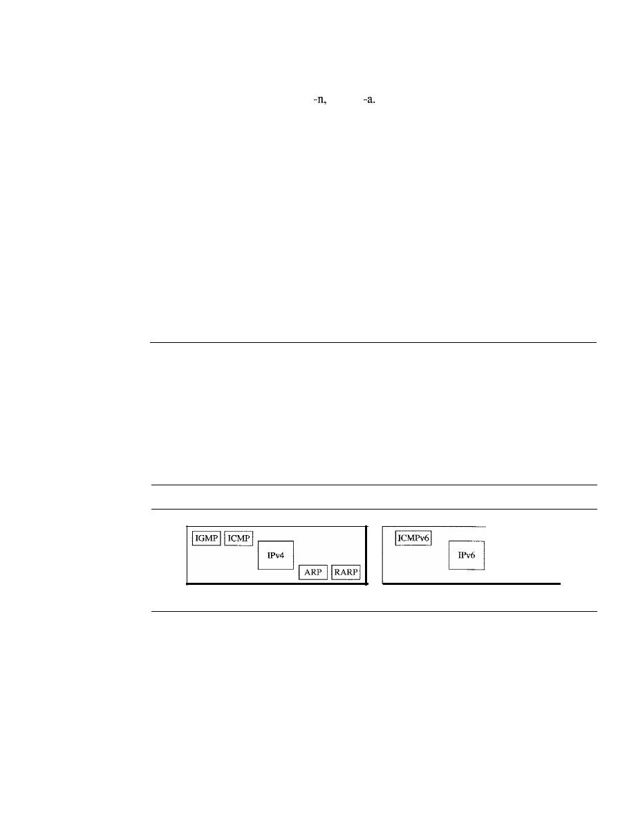
638
CHAPTER
21
NETWORK LAYER: ADDRESS MAPPING, ERROR REPORTING, AND MULTICASTING
Example 21.9
We use
netstat
with three options:
-r, and
The -n option gives the numeric versions of IP
addresses, the -r option gives the routing table, and the -a option gives
all
addresses (unicast and
multicast). Note that we show only the fields relative to our discussion. "Gateway" defines the
router, "Iface" defines the interface.
$
netstat -nra
Kernel IP routing table
Destination
Gateway
153.18.16.0
0.0.0.0
169.254.0.0
0.0.0.0
127.0.0.0
0.0.0.0
224.0.0.0
0.0.0.0
0.0.0.0
153.18.31.254
Mask
255.255.240.0
255.255.0.0
255.0.0.0
224.0.0.0
0.0.0.0
Flags
U
U
U
u
va
Iface
ethO
ethO
10
ethO
ethO
Nate that the multicast address is shown in color. Any packet with a multicast address from
224.0.0.0 to 239.255.255.255 is masked and delivered to the Ethernet interface.
21.4
ICMPv6
We discussed 1Pv6 in Chapter 20. Another protocol that has been modified in version 6 of
the TCPIIP protocol suite is ICMP (ICMPv6). This new version follows the same strategy
and purposes of version 4. ICMPv4 has been modified to make it more suitable for IPv6.
In addition, some protocols that were independent in version 4 are now part of
Internet-
working Control Message Protocol (ICMPv6).
Figure 21.23 compares the network
layer of version 4 to version 6.
Figure 21.23
Comparison of network layers in version
4
and version 6
Network layer in version 4
Network layer in version 6
The ARP and IGMP protocols in version 4 are combined in ICMPv6. The RARP
protocol is dropped from the suite because it was rarely used and BOOTP has the same
functionality.
Just as in ICMPv4, we divide the ICMP messages into two categories. However,
each category has more types of messages than before.
Error Reporting
As we saw in our discussion of version 4, one of the main responsibilities of ICMP is to
report errors. Five types of errors are handled: destination unreachable, packet too big,
time exceeded, parameter problems, and redirection. ICMPv6 forms an error packet,

SECTION 21.4
ICMPv6
639
which is then encapsulated in an IP datagram. This is delivered to the original source of
the failed datagram. Table 21.3 compares the error-reporting messages of ICMPv4
with ICMPv6. The source-quench message is eliminated in version 6 because the priority
and the flow label fields allow the router to control congestion and discard the least
important messages. In this version, there is no need to inform the sender to slow down.
The packet-too-big message is added because fragmentation is the responsibility of the
sender in IPv6.
If
the sender does not make the right packet size decision, the router has
no choice but to drop the packet and send an error message to the sender.
Table 21.3
Comparison of error-reporting messages in ICMPv4 and ICMPv6
Type ofMessage
Version 4
Version 6
Destination unreachable
Yes
Yes
Source quench
Yes
No
Packet too big
No
Yes
Time exceeded
Yes
Yes
Parameter problem
Yes
Yes
Redirection
Yes
Yes
Destination Unreachable
The concept of the destination-unreachable message is exactly the same as described
for ICMP version 4.
Packet Too Big
This is a new type of message added to version 6. If a router receives a datagram that is
larger than the maximum transmission unit (MTU) size of the network through which
the datagram should pass, two things happen. First, the router discards the datagram
and then an ICMP error packet-a packet-too-big message-is sent to the source.
Time Exceeded
This message is similar to the one in version 4.
Parameter Problem
This message is similar to its version 4 counterpart.
Redirection
The purpose of the redirection message is the same as described for version 4.
Query
In addition to error reporting, ICMP can diagnose some network problems. This is
accomplished through the query messages. Four different groups of messages have been
defined: echo request and reply, router solicitation and advertisement, neighbor solicita-
tion and advertisement, and group membership. Table 21.4 shows a comparison between

640
CHAPTER
21
NETWORK LAYER: ADDRESS MAPPING, ERROR REPORTING, AND MULTICASTING
the query messages in versions 4 and 6. Two sets of query messages are eliminated from
ICMPv6: time-stamp request and reply- and address-mask request and reply. The time-
stamp request and reply messages are eliminated because they are implemented in other
protocols such as TCP and because they were rarely used in the past. The address-mask
request and reply messages are eliminated in IPv6 because the subnet section of an
address allows the subscriber to use up to 2
32
-
1 subnets. Therefore, subnet masking, as
defined in IPv4, is not needed here.
Table 21.4
Comparison of query messages in ICMPv4 and ICMPv6
Type ofMessage
Version 4
Version 6
Echo request and reply
Yes
Yes
Timestamp request and reply
Yes
No
Address-mask request and reply
Yes
No
Router solicitation and advertisement
Yes
Yes
Neighbor solicitation and advertisement
ARP
Yes
Group membership
IGMP
Yes
Echo Request and Reply
The idea and format of the echo request and reply messages are the same as those in
version 4.
Router Solicitation and Advertisement
The idea behind the router-solicitation and -advertisement messages is the same as in
version 4.
Neighbor Solicitation and Advertisement
As previously mentioned, the network layer in version 4 contains an independent protocol
called Address Resolution Protocol (ARP). In version 6, this protocol is eliminated, and
its duties are included in ICMPv6. The idea is exactly the same, but the format of the
message has changed.
Group Membership
As previously mentioned, the network layer in version 4 contains an independent protocol
called IGMP. In version 6, this protocol is eliminated, and its duties are included in
ICMPv6. The purpose is exactly the same.
21.5
RECOMMENDED READING
For more details about subjects discussed in this chapter, we recommend the follow-
ing books and site. The items in brackets [...
J
refer to the reference list at the end of
the text.

SECTION21.6
KEYTERMS
641
Books
ARP and RARP are discussed in Chapter 7 of [For06] and Chapters 4 and 5 of [Ste94].
ICMP is discussed in Chapter 9 of [For06] and Chapter 6 of [Ste94]. IGMP is discussed
in Chapter
10 of [For06] and Chapter 13 of [Ste94]. BOOTP and DHCP are discussed in
Chapter 16 of [For06] and Chapter 16 of [Ste94]. ICMPv6 is discussed in Chapter 27 of
[For06].
Site
o
www.ietf.org/rfc.html
Information about RFCs
RFCs
A discussion of ARP and RARP can be found in following RFCs:
826,903,925,1027,1293,1329,1433,1868,1931,2390
A discussion of ICMP can be found in the following RFCs:
777,792,1016,1018,1256,1788,2521
A discussion of IGMP can be found in the following RFCs:
966,988,1054,1112, 1301,1458, 1469,1768,2236,2357,2365,2502,2588
A discussion of BOOTP and DHCP can be found in the following RFCs:
951,1048,1084,1395,1497,1531,1532,1533,1534, 1541, 1542,2131,2132
21.6
KEY TERMS
address-mask-reply message
address-mask-request message
address resolution protocol
(ARP)
Bootstrap Protocol (BOOTP)
delayed response strategy
destination-unreachable message
dynamic configuration protocol
Dynamic Host Configuration Protocol
(DHCP)
dynamic mapping
echo-request and echo-reply messages
error-reporting message
general query message
groupid
group membership
Internet Control Message Protocol
(ICMP)
Internet Group Management Protocol
(IGMP)
Internetworking Control Message
Protocol, version 6 (ICMPv6)
lease
leave report
membership report

642
CHAPTER
21
NETWORK LAYER: ADDRESS MAPPING, ERROR REPORTING, AND MULTICASTING
multicast address
multicast router
multicasting
neighbor-solicitation and advertisement
message
packet-too-big message
parameter-problem message
physical address
proxyARP
query message
query router
redirection message
relay agent
reverse address resolution protocol
(RARP)
router-solicitation and router-
advertisement messages
source-quench message
special query message
static mapping
time-exceeded message
timestamp request and timestamp
reply messages
traceroute
tunneling
21.7
SUMMARY
o
Delivery of a packet to a host or router requires two levels of addresses: logical and
physical. A physical address identifies a host or router at the physical level.
o
Mapping of a logical address to a physical address can be static or dynamic.
o
Static mapping involves a list of logical and physical address correspondences;
maintenance of the list requires high overhead.
o
The address resolution protocol (ARP) is a dynamic mapping method that finds a
physical address, given a logical address.
o
In proxy ARP, a router represents a set of hosts. When an ARP request seeks the
physical address of any host in this set, the router sends its own physical address.
This creates a subnetting effect.
o
Reverse Address Resolution Protocol (RARP) is a form of dynamic mapping in
which a given physical address is associated with a logical address.
o
ICMP sends four pairs of query messages: echo-request and echo-reply, time-stamp
request and reply, address-mask-request and -reply, and router solicitation and
advertisement.
D
The checksum for ICMP is calculated by using both the header and the data fields
of the ICMP message.
D
Packet InterNet Groper
(ping)
is an application program that uses the services of
ICMP to test the reachability of a host.
o
Multicasting is the sending of the same message to more than one receiver
simultaneously.
o
The Internet Group Management Protocol (IGMP) helps multicast routers create and
update a list of loyal members related to a router interface.
o
The three IGMP message types are the query message, the membership report, and
the leave report.

SECTION
21.8
PRACTICE SET
643
D
A delayed response strategy prevents unnecessary traffic on a LAN.
D
The IGMP message is encapsulated in an IP datagram.
D
Most LANs, including Ethernet, support physical multicast addressing.
D
WANs that do not support physical multicast addressing can use a process called
tunneling to send multicast packets.
D
BOOTP and Dynamic Host Configuration Protocol (DHCP) are client/server applica-
tions that deliver vital network information to either diskless computers or computers
at first boot.
D
A BOOTP request is encapsulated in a UDP user datagram.
D
BOOTP, a static configuration protocol, uses a table that maps IP addresses to
physical addresses.
D
A relay agent is a router that helps send local BOOTP requests to remote servers.
D
DHCP is a dynamic configuration protocol with two databases: One is similar to
BOOTP, and the other is a pool of IP addresses available for temporary assignment.
D
The DHCP server issues a lease for an IP address to a client for a specific time.
D
ICMPv6, like version 4, reports errors, handles group memberships, updates specific
router and host tables, and checks the viability of a host.
21.8
PRACTICE SET
Review Questions
1. Is the size of the ARP packet fixed? Explain.
2. What is the size of an ARP packet when the protocol is IPv4 and the hardware is
Ethernet?
3. What is the size of an Ethernet frame carrying an ARP packet in Question 2?
4. What is the broadcast address for Ethernet?
5. Why is there a restriction on the generation of an ICMPv4 message in response to
a failed ICMPv4 error message?
6. What is the purpose of including the IPv4 header and the first 8 bytes of datagram
data in the error-reporting ICMPv4 messages?
7. Give an example of a situation in which a host would never receive a redirection
message.
8. What is the minimum size of an ICMPv4 packet? What is the maximum size of an
ICMPv4 packet?
9. What is the minimum size of an IPv4 packet that carries an ICMPv4 packet? What
is the maximum size?
10. How can we determine if an IPv4 packet is carrying an ICMPv4 packet?
11. What is the minimum size of an Ethernet frame that carries an IPv4 packet which
in turn carries an ICMPv4 packet? What is the maximum size?
12. Why is there no need for the ICMPv4 message to travel outside its own network?

644
CHAPTER 21
NETWORK LAYER: ADDRESS MAPPING, ERROR REPORTING, AND MULTICASTING
Exercises
13. A router with IPv4 address
125.45.23.12 and Ethernet physical address
23:45:AB:4F:67:CD has received a packet for a host destination with IP address
125.11.78.10. Show the entries in theARP request packet sent by the router. Assume
no subnetting.
14. Show the entries in the ARP packet sent in response to Exercise 13.
15. Encapsulate the result of Exercise 13 in a data link frame. Fill in all the fields.
16. Encapsulate the result of Exercise 14 in a data link frame. Fill in all the fields.
17. Host A sends a datagram to host B. Host B never receives the datagram, and host A
never receives notification of failure. Give two different explanations of what might
have happened.
18. Calculate the checksum for the following ICMP packet:
Type: Echo Request
Identifier: 123
Sequence number: 25
Message: Hello
19. A router receives an IPv4 packet with source IP address 130.45.3.3 and destination
IP address 201.23.4.6. The router cannot find the destination IP address in its routing
table. Which ICMPv4 message should be sent?
20. TCP receives a segment with destination port address 234. TCP checks and cannot
find an open port for this destination. Which ICMPv4 message should be sent?
21. A multicast address for a group is 231.24.60.9. What is its 48-bit Ethernet address
for a LAN using TCPIIP?
22. If a router has 20 entries in its group table, should it send 20 different queries period-
ically or just one? Explain your answer.
23. If a host wants to continue membership in five groups, should it send five different
membership report messages or just one?
24. A router on an Ethernet network has received a multicast IP packet with groupid
226.17.18.4. When the host checks its multicast group table, it finds this address.
Show how the router sends this packet to the recipients by encapsulating the IP
packet in an Ethernet frame. Show all the entries of the Ethernet frame. The outgoing
IP address of the router is 185.23.5.6, and its outgoing physical address is
4A224512E1E2. Does the router need the services of ARP?
25. A host with IPv4 address 114.45.7.9 receives an IGMP query. When it checks its
group table, it finds no entries. What action should the host take? Should it send
any messages?
26. A host with IPv4 address 222.5.7.19 receives an IGMP query. When it checks its
routing table, it finds two entries in its table: 227.4.3.7 and 229.45.6.23. What
action should the host take? Should it send any messages? If so, what type and how
many?
27. How many multicast addresses can be supported for the IPv4 protocol in Ethernet?
How many multicast addresses can be supported by the IPv4 protocol? What is the
size of address space lost when we transform a multicast IPv4 address to an Ethernet
multicast address?
28. Change the following IPv4 multicast addresses to Ethernet multicast addresses.
How many of them specify the same Ethernet address?

SECTION
21.8
PRACTICE SET
645
a.
224.18.72.8
b. 235.18.72.8
c. 237.18.6.88
d. 224.88.12.8
Research Activities
29. Use the ping program to test your own computer (loopback).
30. Use the ping program to test a host inside the United States.
31. Use the ping program to test a host outside the United States.
32. Use traceroute (or tracert) to find the route from your computer to a computer in a
college or university.
33. Use netstat to find out if your server supports multicast addressing.
34. DHCP uses several messages such as DHCPREQUEST, DHCPDECLINE,
DHCPACK, DHCPNACK, and DHCPRELEASE. Find the purpose of these
messages.


CHAPTER 22
Network Layer:
Delivery, Forwarding, and Routing
This chapter describes the delivery, forwarding, and routing of IP packets to their final
destinations.
Delivery
refers to the way a packet is handled by the underlying networks
under the control of the network layer.
Forwarding
refers to the way a packet is deliv-
ered to the next station.
Routing
refers to the way routing tables are created to help in
forwarding.
Routing protocols
are used to continuously update the routing tables that are con-
sulted for forwarding and routing. In this chapter, we also briefly discuss common uni-
cast and
multicast routing
protocols.
22.1
DELIVERY
The network layer supervises the handling of the packets by the underlying physical
networks.We define this handling as the delivery of a packet.
Direct Versus Indirect Delivery
The delivery of a packet to its final destination is accomplished by using two different
methods of delivery, direct and indirect, as shown in Figure 22.1.
Direct Delivery
In a
direct delivery,
the final destination of the packet is a host connected to the same
physical network as the deliverer. Direct delivery occurs when the source and destina-
tion of the packet are located on the same physical network or when the delivery is
between the last router and the destination host.
The sender can easily determine if the delivery is direct.
It
can extract the network
address of the destination (using the mask) and compare this address with the addresses
of the networks to which it is connected. If a match is found, the delivery is direct.
Indirect Delivery
If
the destination host is not on the same network as the deliverer, the packet is deliv-
ered indirectly. In an
indirect delivery,
the packet goes from router to router until it
reaches the one connected to the same physical network as its final destination. Note
647
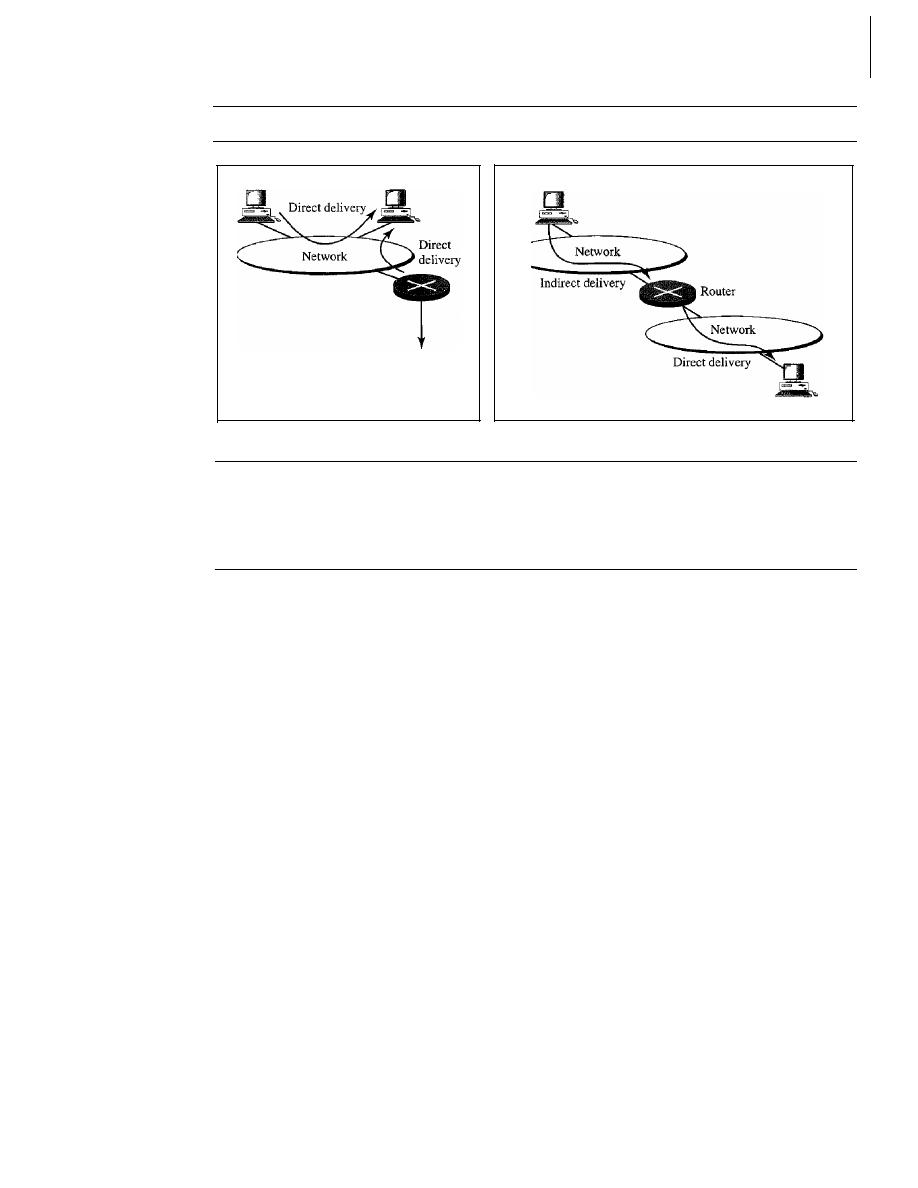
648
CHAPTER
22
NETWORK LAYER: DELIVERY, FORWARDING, AND ROUTING
Figure 22.1
Direct and indirect delivery
Host
Host
Host (source)
To the rest
of the Internet
a. Direct delivery
Host (destination)
b. Indirect and direct delivery
that a delivery always involves one direct delivery but zero or more indirect deliveries.
Note also that the last delivery is always a direct delivery.
22.2
FORWARDING
Forwarding means to place the packet in its route to its destination. Forwarding
requires a host or a router to have a routing table. When a host has a packet to send or
when a router has received a packet to be forwarded, it looks at this table to find the
route to the final destination. However, this simple solution is impossible today in an
internetwork such as the Internet because the number of entries needed in the routing
table would make table lookups inefficient.
Forwarding Techniques
Several techniques can make the size of the routing table manageable and also handle
issues such as security. We briefly discuss these methods here.
Next-Hop Method Versus Route Method
One technique to reduce the contents of a routing table is called the next-hop method.
In this technique, the routing table holds only the address of the next hop instead
of information about the complete route (route method). The entries of a routing table
must be consistent with one another. Figure 22.2 shows how routing tables can be sim-
plified by using this technique.
Network-Specific Method Versus Host-Specific Method
A second technique to reduce the routing table and simplify the searching process is
called the network-specific method. Here, instead of having an entry for every desti-
nation host connected to the same physical network (host-specific method), we have
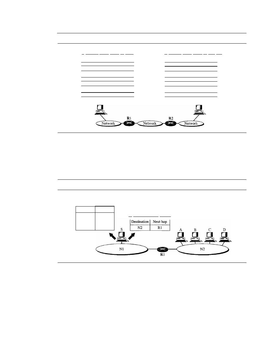
SECTION
22.2
FORWARDING
649
Figure 22.2
Route method versus next-hop method
a. Routing tables based on route
Destination
Route
HostB
RI, R2, host B
Routing table
for host
A
b. Routing tables based on next hop
Destination
Next hop
Host B
Rl
Destination
HostB
Destination
HostB
Host A
Route
R2, host B
Route
HostB
Routing table
for Rl
Routing table
for R2
Destination
HostB
Destination
Host B
Next hop
R2
Next hop
HostB
only one entry that defines the address of the destination network itself. In other words,
we treat all hosts connected to the same network as one single entity. For example, if
1000 hosts are attached to the same network, only one entry exists in the routing table
instead of 1000. Figure 22.3 shows the concept.
Figure 22.3
Host-specific versus network-specific method
Routing table for host S based
on host-specific method
Destination
Next hop
A
Rl
B
Rl
C
Rl
D
Rl
Routing table for host S based
on network-specific method
Host-specific routing is used for purposes such as checking the route or providing
security measures.
Default Method
Another technique to simplify routing is called the
default method.
In Figure 22.4 host
A is connected to a network with two routers. Router Rl routes the packets to hosts
connected to network N2. However, for the rest of the Internet, router R2 is used. So
instead of listing all networks in the entire Internet, host A can just have one entry
called the default (normally defined as network address 0.0.0.0).
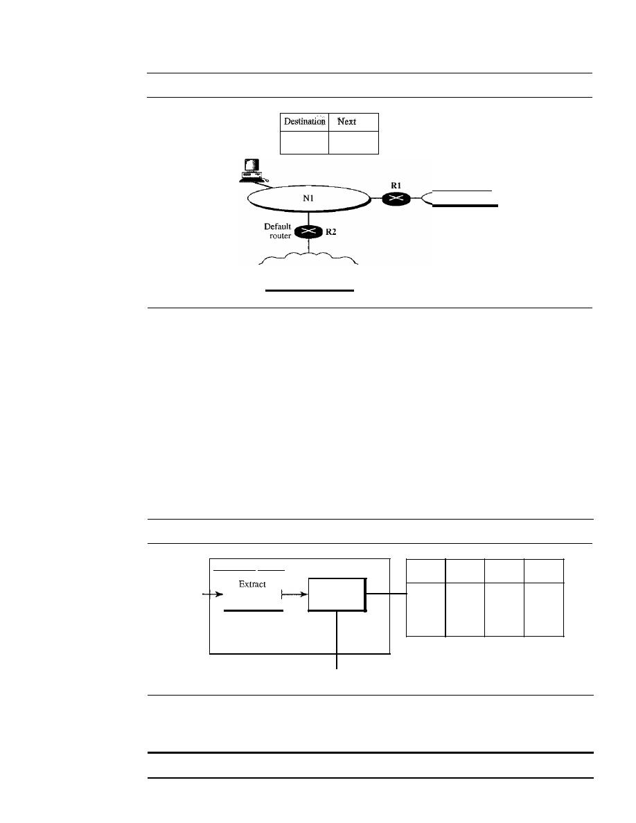
650
CHAPTER
22
NETWORK LAYER: DELIVERY, FORWARDING, AND ROUTING
Figure 22.4
Default method
Host A
hop ,
N2
Rl
Any other
R2
Routing table
for host A
N2
Rest of the Internet
Forwarding Process
Let us discuss the forwarding process. We assume that hosts and routers use classless
addressing because classful addressing can be treated as a special case of classless
addressing. In classless addressing, the routing table needs to have one row of informa-
tion for each block involved. The table needs to be searched based on the network
address (first address in the block). Unfortunately, the destination address in the packet
gives no clue about the network address. To solve the problem, we need to include the
mask
(In)
in the table; we need to have an extra column that includes the mask for the
corresponding block. Figure 22.5 shows a simple forwarding module for classless
addressing.
Figure 22.5
Simplified forwarding module in classless address
Forwarding module
Packet
destination
address
Search
table
Mask
(In)
Network Next-hop
Interface
address
address
Next-hop address
and
interface number
ToARP
Note that we need at least four columns in our routing table; usually there are more.
In classless addressing, we need at least four colwnns in a routing table.
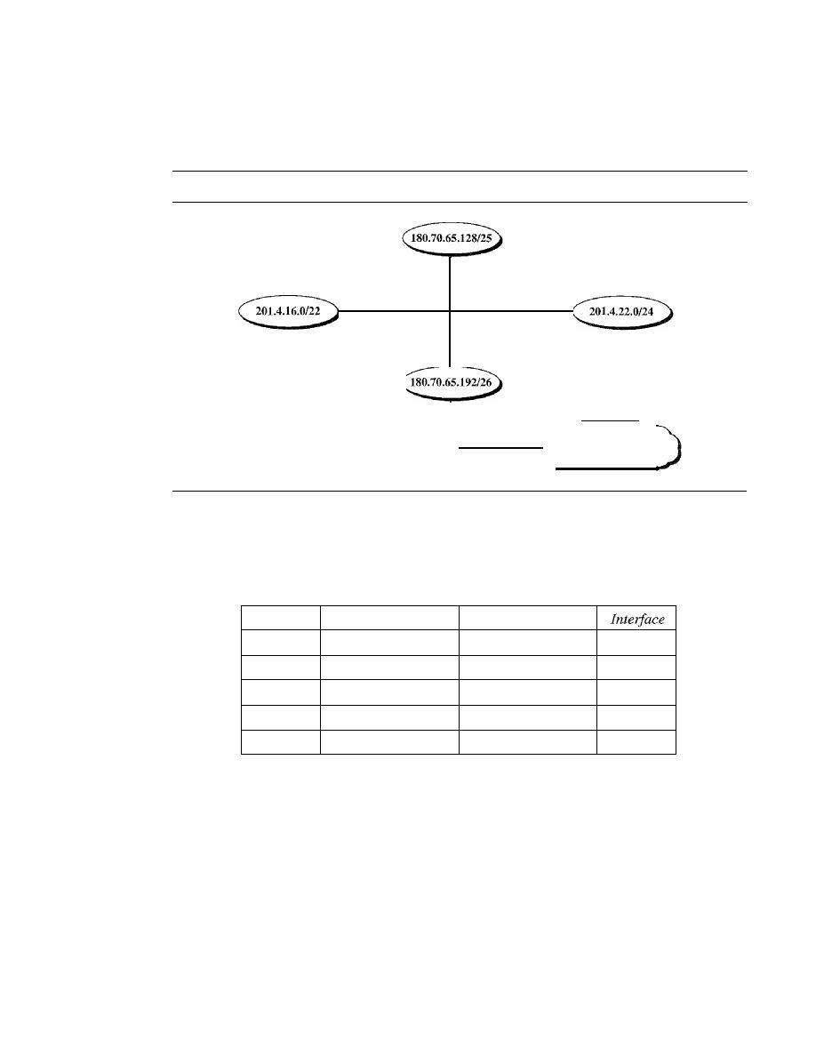
SECTION
22.2
FORWARDING
651
Example 22.1
Make a routing table for router Rl, using the configuration in Figure 22.6.
Figure 22.6
Configurationfor Example 22.1
180.70.65.135/25
ml
mO
201.4.16.2/22
201.4.22.3/24
m2
Rl
180.70.65.194/26
180.70.65.200/26
Rest of the Intemet
Solution
Table 22.1 shows the corresponding table.
Table 22.1
Routing table for router RI in Figure 22.6
Mask
Network Address
Next Hop
/26
180.70.65.192
-
m2
/25
180.70.65.128
-
mO
/24
201.4.22.0
-
m3
/22
201.4.16.0
....
ml
Any
Any
180.70.65.200
m2
Example 22.2
Show the forwarding process if a packet arrives at Rl in Figure 22.6 with the destination address
180.70.65.140.
Solution
The router performs the following steps:
1.
The first mask (/26) is applied to the destination address. The result is 180.70.65.128, which
does not match the corresponding network address.
2. The second mask (/25) is applied to the destination address. The result is 180.70.65.128,
which matches the corresponding network address. The next-hop address (the destination
address of the packet in this case) and the interface number mO are passed to ARP for further
processing.

652
CHAPTER 22
NETWORK LAYER: DELIVERY, FORWARDING, AND ROUTING
Example 22.3
Show the forwarding process if a packet arrives at R1 in Figure 22.6 with the destination address
201.4.22.35.
Solution
The router performs the following steps:
I.
The first mask (/26) is applied to the destination address. The result is 201.4.22.0, which
does not match the corresponding network address (row 1).
2. The second mask (/25) is applied to the destination address. The result is 201.4.22.0, which
does not match the corresponding network address (row 2).
3. The third mask (/24) is applied to the destination address. The result is 201.4.22.0, which
matches the corresponding network address. The destination address of the packet and the
interface number m3 are passed to ARP.
Example 22.4
Show the forwarding process if a packet arrives at R1 in Figure 22.6 with the destination address
18.24.32.78.
Solution
This time all masks are applied, one by one, to the destination address, but no matching network
address is found. When it reaches the end of the table, the module gives the next-hop address
180.70.65.200 and interface number m2 to ARP. This is probably an outgoing package that needs
to be sent, via the default router, to someplace else in the Internet.
Address Aggregatioll
When we use classless addressing, it is likely that the number of routing table entries
will increase. This is so because the intent of classless addressing is to divide up the
whole address space into manageable blocks. The increased size of the table results in
an increase in the amount of time needed to search the table. To alleviate the problem,
the idea of
address aggregation
was designed. In Figure 22.7 we have two routers.
Router Rl is connected to networks of four organizations that each use 64 addresses.
Router R2 is somewhere far from Rl. Router Rl has a longer routing table because each
packet must be correctly routed to the appropriate organization. Router R2, on the other
hand, can have a very small routing table. For R2, any packet with destination 140.24.7.0
to 140.24.7.255 is sent out from interface mO regardless of the organization number. This
is called address aggregation because the blocks of addresses for four organizations are
aggregated into one larger block. Router R2 would have a longer routing table if each
organization had addresses that could not be aggregated into one block.
Note that although the idea of address aggregation is similar to the idea of subnet-
ting, we do not have a common site here; the network for each organization is indepen-
dent. In addition, we can have several levels of aggregation.
Longest Mask Matching
What happens if one of the organizations in Figure 22.7 is not geographically close to
the other three? For example, if organization 4 cannot be connected to router Rl for
some reason, can we still use the idea of address aggregation and still assign block
140.24.7.192/26 to organization 4?
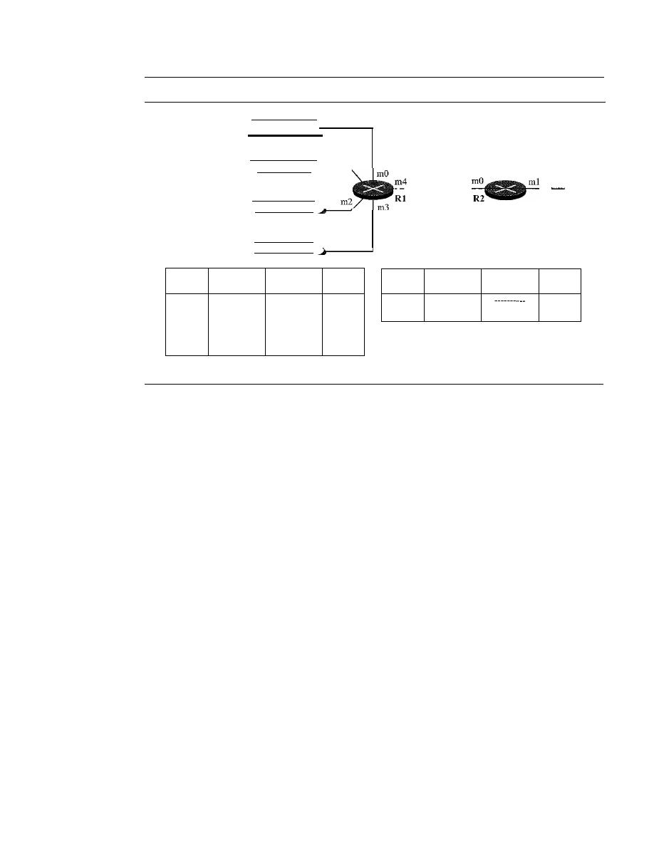
SECTION
22.2
FORWARDING
653
Figure 22.7
Address aggregation
Organization 1
140.24.7.0/26
Somewhere
in the Internet
ml
Organization 3
140.24.7.128/26
Organization 2
140.24.7.64/26
Organization 4
140.24.7.192/26
Mask
Network
Next-hop
Interface
address
address
/26
140.24.7.0
----------
mO
/26
140.24.7.64
----------
ml
/26
140.24.7.128
----------
m2
/26
140.24.7.192
----------
m3
/0
0.0.0.0
Default
m4
Mask
Network
Next-hop
Interface
address
address
/24
140.24.7.0
mO
/0
0.0.0.0
Default
ml
Routmg table for R2
Routing table for Rl
The answer is yes because routing in classless addressing uses another principle,
longest mask matching. This principle states that the routing table is sorted from the
longest mask to the shortest mask. In other words, if there are three masks
127, 126,
and
124,
the mask /27 must be the first entry and
124
must be last. Let us see if this principle
solves the situation in which organization 4 is separated from the other three organiza-
tions. Figure 22.8 shows the situation.
Suppose a packet arrives for organization 4 with destination address 140.24.7.200.
The first mask at router R2 is applied, which gives the network address 140.24.7.192.
The packet is routed correctly from interface ml and reaches organization 4.
If,
how-
ever, the routing table was not stored with the longest prefix first, applying the /24 mask
would result in the incorrect routing of the packet to router Rl.
Hierarchical Routing
To solve the problem of gigantic routing tables, we can create a sense of hierarchy in
the routing tables. In Chapter 1, we mentioned that the Internet today has a sense of
hierarchy. We said that the Internet is divided into international and national ISPs.
National ISPs are divided into regional ISPs, and regional ISPs are divided into local
ISPs. If the routing table has a sense of hierarchy like the Internet architecture, the rout-
ing table can decrease in size.
Let us take the case of a local ISP. A local ISP can be assigned a single, but large
block of addresses with a certain prefix length. The local ISP can divide this block into
smaller blocks of different sizes and can assign these to individual users and organiza-
tions, both large and small. If the block assigned to the local ISP starts with a.b.c.dln,
the ISP can create blocks starting with eJ.g.h/m, where
m
may vary for each customer
and is greater than n.
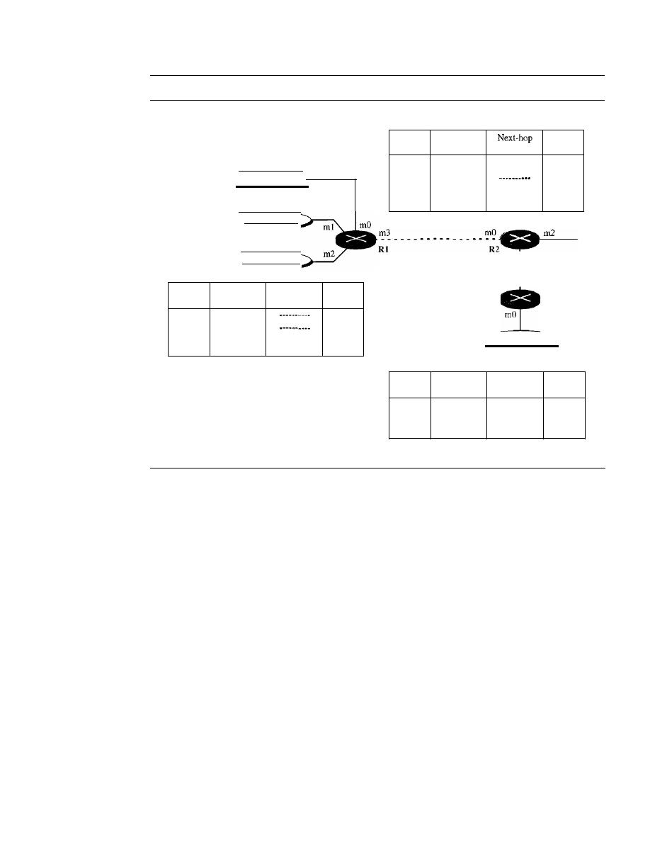
654
CHAPTER
22
NETWORK LAYER: DELIVERY, FORWARDING, AND ROUTING
Figure 22.8
Longest mask matching
Routing table for R2
140.24.7.192/26
Organization 4
R3
ml
Mask
Network
Interface
address
address
/26
140.24.7.192
----------
ml
/24
140.24.7.0
mO
I??
???????
?????????
ml
/0
0.0.0.0
Default
m2
To other networks
- - - - I
Iml
I
I
I
ml
l
Organization 3
140.24.7.128/26
Organization 2
140.24.7.64/26
Routmg table for RI
Mask
Network
Next-hop
Interface
address
address
/26
140.24.7.0
mO
/26
140.24.7.64
ml
/26
140.24.7.128
----------
m2
/0
0.0.0.0
Default
m3
Organization 1
140.24.7.0/26
Mask
Network
Next-hop
Interface
address
address
/26
140.24.7.192
----------
rnO
I??
???????
?????????
rnl
/0
0.0.0.0
Default
rn2
Routing table for R3
How does this reduce the size of the routing table? The rest of the Internet does not
have to be aware of this division. All customers of the local ISP are defined as a.b.c.dln to
the rest of the Internet. Every packet destined for one of the addresses in this large block is
routed to the local ISP. There is only one entry in every router
in
the world for all these cus-
tomers. They all belong to the same group. Of course, inside the local ISp, the router must
recognize the subblocks and route the packet to the destined customer.
If
one of the cus-
tomers is a large organization, it also can create another level of hierarchy by subnetting
and dividing its subblock into smaller subblocks (or sub-subblocks). In classless routing,
the levels of hierarchy are unlimited so long as we follow the rules of classless addressing.
Example 22.5
As an example of hierarchical routing, let us consider Figure 22.9. A regional ISP is granted
16,384 addresses starting from 120.14.64.0. The regional ISP has decided to divide this block
into four subblocks, each with 4096 addresses. Three of these subblocks are assigned to three
local ISPs; the second subblock is reserved for future use. Note that the mask for each block is
120
because the original block with mask /18 is divided into 4 blocks.
The first local ISP has divided its assigned subblock into 8 smaller blocks and assigned each
to a small ISP. Each small ISP provides services to 128 households (HOOI to HI28), each using
four addresses. Note that the mask for each small ISP is now
123
because the block is further
divided into 8 blocks. Each household has a mask of
130,
because a household has only four
addresses (2
32
-
30
is 4).
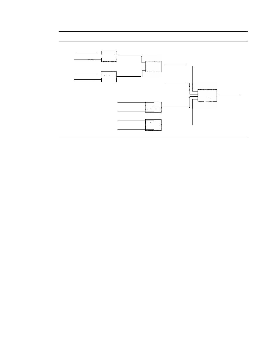
SECTION
22.2
FORWARDING
655
Figure 22.9
Hierarchical routing with ISPs
120.14.64.0118
Total 16384
120.14.80.0/20
Tota14096
120.14.64.0/20
Tota14096
120.14.64.0/23
Total 512
LOrgOl
120.14.96.0/22
·
120.14.96.0/20
·
LOrg04
·
Total 4096
SOrg 01
120.14.112.0/24
•
120.14.112.0120
·
SOrg 16
•
Total 4096
H 128
__
120.14.78.0/23
H 001
120.14.78.0/30
Total 512
H 001 120.14.64.0/30
H
128
The second local ISP has divided its block into 4 blocks and has assigned the addresses to
four large organizations (LOrg01 to LOrg04). Note that each large organization has 1024 addresses,
and the mask is /22.
The third local ISP has divided its block into 16 blocks and assigned each block to a
small organization (SOrg01 to SOrg16). Each small organization has 256 addresses, and the
mask is /24.
There is a sense of hierarchy in this configuration. All routers in the Internet send a packet
with destination address 120.14.64.0 to 120.14.127.255 to the regional ISP.
The regional ISP sends every packet with destination address 120.14.64.0 to 120.14.79.255
to local ISPl. Local ISP1 sends every packet with destination address 120.14.64.0 to 120.14.64.3
to H001.
Geographical Routing
To decrease the size of the routing table even further, we need to extend hierarchical
routing to include geographical routing. We must divide the entire address space into a
few large blocks. We assign a block to North America, a block to Europe, a block to
Asia, a block to Africa, and so on. The routers of ISPs outside Europe will have only
one entry for packets to Europe in their routing tables. The routers of ISPs outside
North America will have only one entry for packets to North America in their routing
tables. And so on.
Routing Table
Let us now discuss routing tables. A host or a router has a routing table with an entry
for each destination, or a combination of destinations, to route IP packets. The routing
table can be either static or dynamic.
Static Routing Table
A static routing table contains information entered manually. The administrator enters
the route for each destination into the table. When a table is created, it cannot update
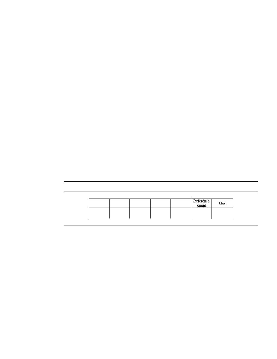
656
CHAPTER
22
NETWORK LAYER: DELIVERY, FORWARDING, AND ROUTING
automatically when there is a change in the Internet. The table must be manually altered
by the administrator.
A static routing table can be used in a small internet that does not change very often,
or in an experimental internet for troubleshooting. It is poor strategy to use a static routing
table in a big internet such as the Internet.
Dynamic Routing Table
A
dynamic routing table
is updated periodically by using one of the dynamic routing
protocols such as RIP, OSPF, or BGP. Whenever there is a change in the Internet, such
as a shutdown of a router or breaking of a link, the dynamic routing protocols update all
the tables in the routers (and eventually in the host) automatically.
The routers in a big internet such as the Internet need to be updated dynamically
for efficient delivery of the IP packets. We discuss in detail the three dynamic routing
protocols later in the chapter.
Format
As mentioned previously, a routing table for classless addressing has a minimum of
four columns. However, some of today's routers have even more columns. We should
be aware that the number of columns is vendor-dependent, and not all columns can be
found in all routers. Figure 22.10 shows some common fields in today's routers.
Figure 22.10
Common fields in a routing table
Mask
Network
address
Next-hop
address
Interlace
o
Mask.
This field defines the mask applied for the entry.
o
Network address.
This field defines the network address to which the packet is
finally delivered. In the case of host-specific routing, this field defines the address
of the destination host.
o
Next-hop address.
This field defines the address of the next-hop router to which
the packet is delivered.
D
Interface.
This field shows the name of the interface.
D
Flags.
This field defines up to five flags. Flags are on/off switches that signify
either presence or absence. The five flags are U (up), G (gateway), H (host-specific),
D (added by redirection), and M (modified by redirection).
a. U
(up).
The U flag indicates the router is up and running.
If
this flag is not present,
it means that the router is down. The packet cannot be forwarded and is discarded.
b. G
(gateway).
The G flag means that the destination is in another network. The
packet is delivered to the next-hop router for delivery (indirect delivery). When
this flag is missing, it means the destination is in this network (direct delivery).

SECTION
22.2
FORWARDING
657
c. H
(host-specific).
The H flag indicates that the entry in the network address
field is a host-specific address. When it is missing, it means that the address is
only the network address of the destination.
d. D
(added
by
redirection).
The D flag indicates that routing information for this
destination has been added to the host routing table by a redirection message
from ICMP. We discussed redirection and the ICMP protocol in Chapter 21.
e. M
(modified
by
redirection).
The M flag indicates that the routing information
for this destination has been modified by a redirection message from ICMP. We
discussed redirection and the ICMP protocol in Chapter 21.
o
Reference count.
This field gives the number of users of this route at the moment.
For example, if five people at the same time are connecting to the same host from
this router, the value of this column is 5.
o
Use.
This field shows the number of packets transmitted through this router for the
corresponding destination.
Utilities
There are several utilities that can be used to find the routing information and the con-
tents of a routing table. We discuss
netstat and ifconfig.
Example 22.6
One utility that can be used to find the contents of a routing table for a host or router is netstat in
UNIX or LINUX. The following shows the list of the contents of a default server. We have used
two options, r and n. The option r indicates that we are interested in the routing table, and the
option n indicates that we are looking for numeric addresses. Note that this is a routing table for a
host, not a router. Although we discussed the routing table for a router throughout the chapter, a host
also needs a routing table.
$ netstat-rn
Kernel IP routing table
Destination
Gateway
153.18.16.0
0.0.0.0
127.0.0.0
0.0.0.0
0.0.0.0
153.18.31.254
Mask
255.255.240.0
255.0.0.0
0.0.0.0
Flags
U
U
UO
Iface
ethO
10
ethO
Note also that the order of columns is different from what we showed. The destination column
here defines the network address. The term gateway used by UNIX is synonymous with router. This
column acmally defines the address of the next hop. The value 0.0.0.0 shows that the delivery is
direct. The last entry has a flag of G, which means that the destination can be reached through a
router (default router). The Iface defines the interface. The host has only one real interface, ethO,
which means interface 0 connected to an Ethernet network. The second interface, la, is actually a
virmalloopback interface indicating that the host accepts packets with loopback address 127.0.0.0.
More information about the IP address and physical address of the server can be found by
using the ifconfig command on the given interface (ethO).
$ ifconfig ethO
ethO Link encap:Ethemet HWaddr 00:BO:DO:DF:09:5D
inet addr:153.18.17.11 Bcast: 153.18.31.255 Mask:255.255.240.0
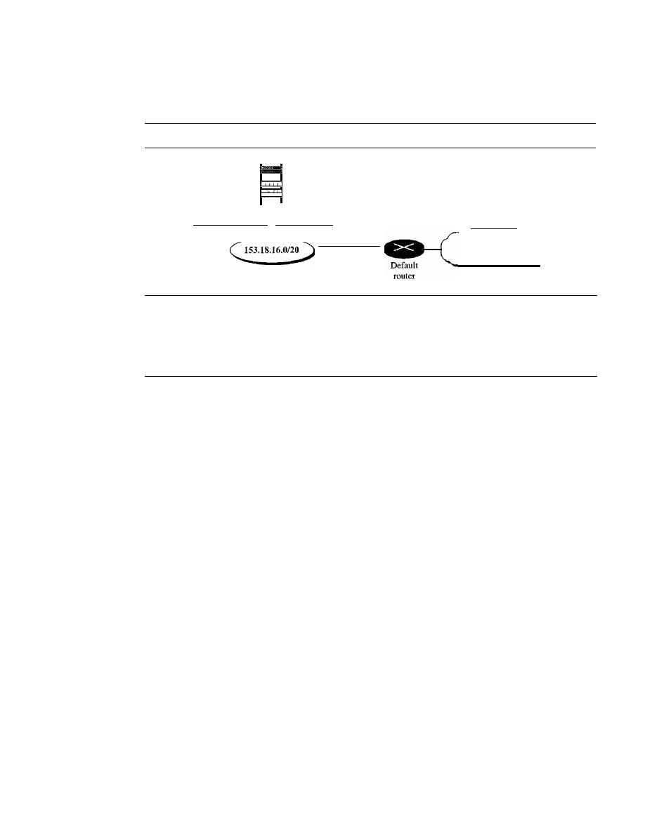
658
CHAPTER
22
NETWORK IAYER: DELIVERY, FORWARDING, AND ROUTING
From the above information, we can deduce the configuration of the server, as shown in
Figure 22.11.
Figure 22.11
Configuration of the server for Example 22.6
-
ethO
00:BO:DO:DF:09:5D 153.18.17.ll/20
153.18.31.254/20
Rest of the Internet
Note that the ifconfig command gives us the IP address and the physical (hardware) address
of the interface.
22.3
UNICAST ROUTING PROTOCOLS
A routing table can be either static or dynamic. A static table is one with manual entries.
A dynamic table, on the other hand, is one that is updated automatically when there is a
change somewhere in the internet. Today, an internet needs dynamic routing tables. The
tables need to be updated as soon as there is a change in the internet. For instance, they
need to be updated when a router is down, and they need to be updated whenever a better
route has been found.
Routing protocols have been created in response to the demand for dynamic routing
tables. A routing protocol is a combination of rules and procedures that lets routers in
the internet inform each other of changes.
It
allows routers to share whatever they know
about the internet or their neighborhood. The sharing of information allows a router in
San Francisco to know about the failure of a network in Texas. The routing protocols
also include procedures for combining information received from other routers.
Optimization
A router receives a packet from a network and passes it to another network. A router is
usually attached to several networks. When
it
receives a packet, to which network
should it pass the packet? The decision is based on optimization: Which of the available
pathways is the optimum pathway? What is the definition of the term optimum?
One approach is to assign a cost for passing through a network. We call this cost a
metric. However, the metric assigned to each network depends on the type of proto-
col. Some simple protocols, such as the Routing Information Protocol (RIP), treat all
networks as equals. The cost of passing through a network is the same;
it
is one hop
count. So if a packet passes through 10 networks to reach the destination, the total cost
is 10 hop counts.
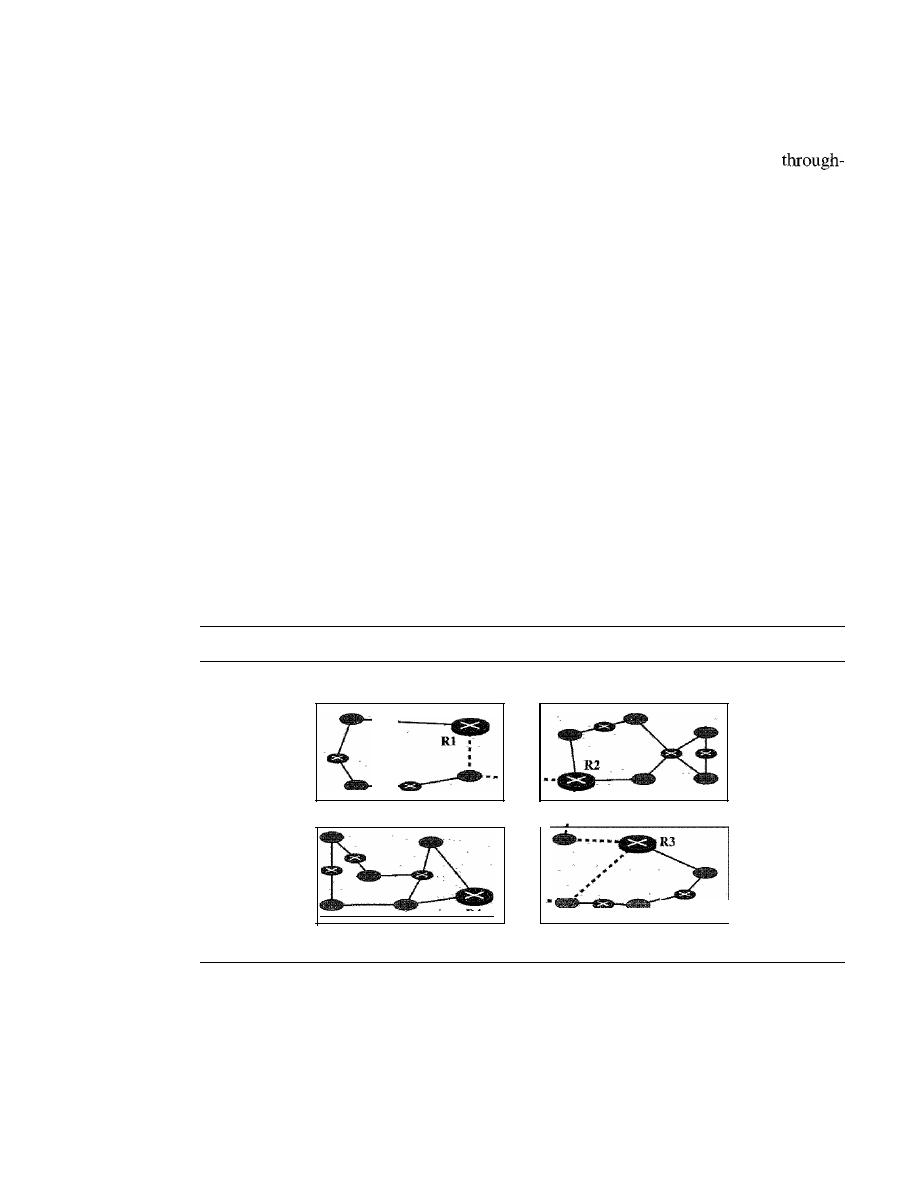
SECTION
22.3
UNICAST ROUTING PROTOCOLS
659
Other protocols, such as Open Shortest Path First (OSPF), allow the administrator to
assign a cost for passing through a network based on the type of service required. A route
through a network can have different costs (metrics). For example, if maximum
put is the desired type of service, a satellite link has a lower metric than a fiber-optic line.
On the other hand, if minimum delay is the desired type of service, a fiber-optic line has
a lower metric than a satellite link. Routers use routing tables to help decide the best
route. OSPF protocol allows each router to have several routing tables based on the
required type of service.
Other protocols define the metric in a totally different way. In the Border Gateway
Protocol (BGP), the criterion is the policy, which can be set by the administrator. The
policy defines what paths should be chosen.
Intra- and Interdomain Routing
Today, an internet can be so large that one routing protocol cannot handle the task of
updating the routing tables of all routers. For this reason, an internet is divided into
autonomous systems. An
autonomous system
(AS) is a group of networks and routers
under the authority of a single administration. Routing inside an autonomous system is
referred to as
intradomain routing.
Routing between autonomous systems is referred
to as
interdomain routing.
Each autonomous system can choose one or more intrado-
main routing protocols to handle routing inside the autonomous system. However, only
one interdomain routing protocol handles routing between autonomous systems (see
Figure 22.12).
Figure 22.12
Autonomous systems
Autonomous system
Autonomous system
.
R4
Autonomous system
···
....
Autonomous system
Several intradomain and interdomain routing protocols are in use. In this section,
we cover only the most popular ones. We discuss two intradomain routing protocols:
distance vector and link state. We also introduce one interdomain routing protocol: path
vector (see Figure 22.13).
Routing Information Protocol (RIP)
is an implementation of the distance vector
protocol.
Open Shortest Path First (OSPF)
is an implementation of the link state proto-
col.
Border Gateway Protocol (BGP)
is an implementation of the path vector protocol.
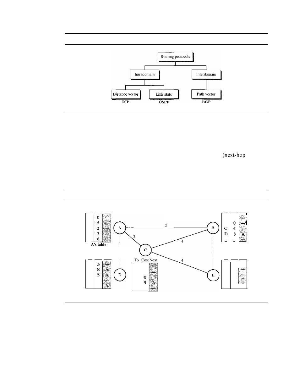
660
CHAPTER
22
NETWORK LAYER: DELIVERY, FORWARDING, AND ROUTING
Figure 22.13
Popular routing protocols
Distance Vector Routing
In
distance vector routing,
the least-cost route between any two nodes is the route
with minimum distance. In this protocol, as the name implies, each node maintains a
vector (table) of minimum distances to every node. The table at each node also guides
the packets to the desired node by showing the next stop in the route
routing).
We can think of nodes as the cities in an area and the lines as the roads connecting
them. A table can show a tourist the minimum distance between cities.
In Figure 22.14, we show a system of five nodes with their corresponding tables.
Figure 22.14
Distance vector routing tables
D's table
E's table
To Cost Next
A
B
C
D
E
To Cost Next
A
5
B
E
3
B's table
3
e's
table
A
2
B
4
C
D
E
4
o
9
3
A
B
C
D
E
A
B
C
D
E
To Cost Next
To Cost Next
The table for node A shows how we can reach any node from this node. For exam-
ple, our least cost to reach node E is 6. The route passes through C.
Initialization
The tables in Figure 22.14 are stable; each node knows how to reach any other node
and the cost. At the beginning, however, this is not the case. Each node can know only
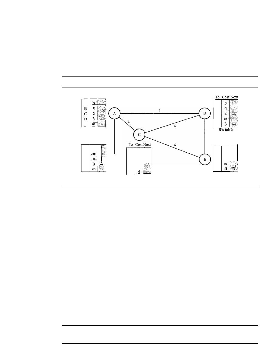
SECTION
22.3
UNICAST ROUTING PROTOCOLS
661
the distance between itself and its immediate neighbors, those directly connected to it.
So for the moment, we assume that each node can send a message to the immediate
neighbors and find the distance between itself and these neighbors. Figure 22.15 shows
the initial tables for each node. The distance for any entry that is not a neighbor is
marked as infinite (unreachable).
Figure 22.15
Initialization of tables in distance vector routing
3
To Cost Next
A
E
A's table
To Cost Next
A
3
B
C
D
E
D's table
D
C's table
3
A
B
C
D
E
To Cost Next
E's
table
Sharing
The whole idea of distance vector routing is the sharing of information between neigh-
bors. Although node A does not know about node E, node C does. So if node C shares
its routing table with A, node A can also know how to reach node E. On the other hand,
node C does not know how to reach node D, but node A does.
If
node A shares its rout-
ing table with node C, node C also knows how to reach node D. In other words, nodes
A and C, as immediate neighbors, can improve their routing tables if they help each
other.
There is only one problem. How much of the table must be shared with each
neighbor? A node is not aware of a neighbor's table. The best solution for each node
is to send its entire table to the neighbor and let the neighbor decide what part to
use and what part to discard. However, the third column of a table (next stop) is not
useful for the neighbor. When the neighbor receives a table, this column needs to
be replaced with the sender's name.
If
any of the rows can be used, the next node is
the sender of the table. A node therefore can send only the first two columns of its
table to any neighbor. In other words, sharing here means sharing only the first two
columns.
In
distance vector routing, each node shares its routing table with its
immediate neighbors periodically and when there is a change.
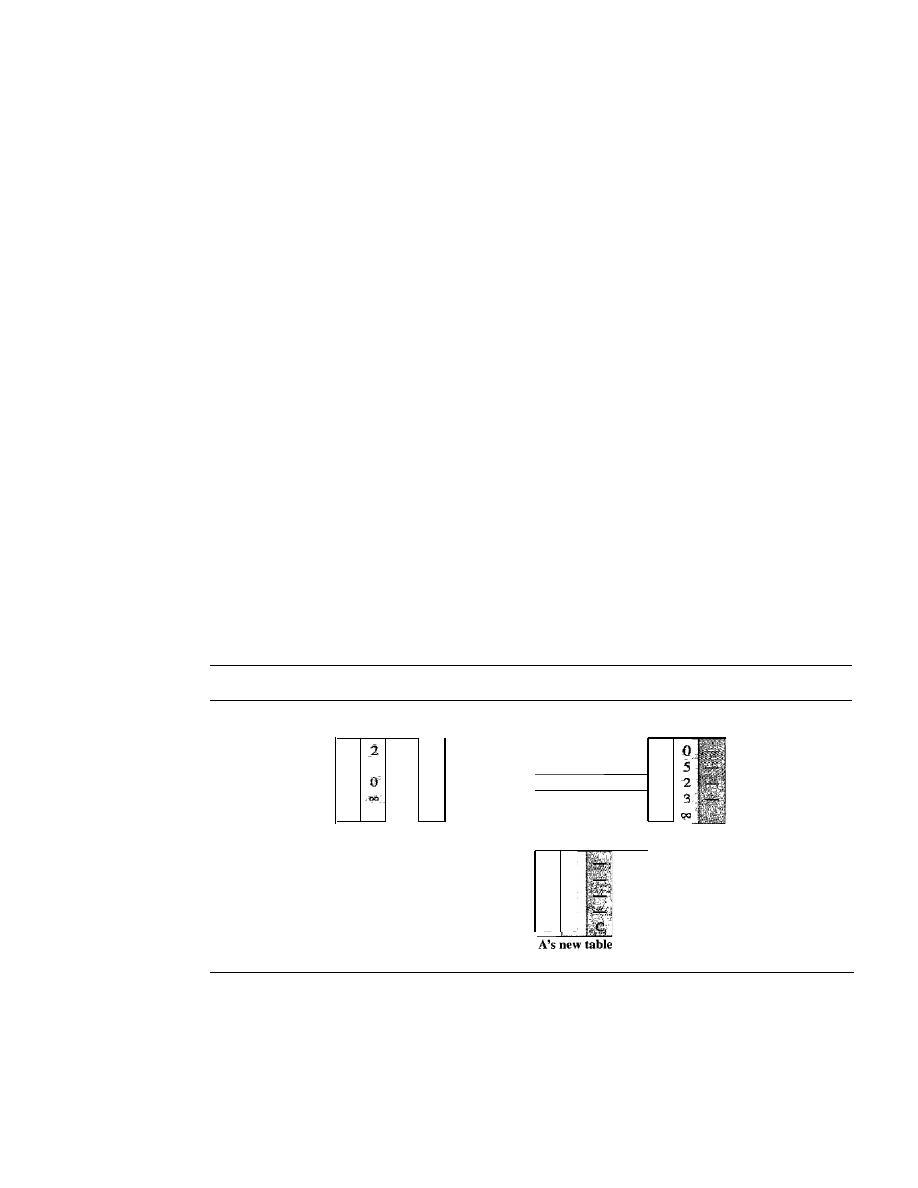
662
CHAPTER
22
NETWORK LAYER: DELIVERY, FORWARDING, AND ROUTING
Updating
When a node receives a two-column table from a neighbor, it needs to update its rout-
ing table. Updating takes three steps:
1. The receiving node needs to add the cost between itself and the sending node
to each value in the second column. The logic is clear.
If
node C claims that its
distance to a destination is
x mi, and the distance between A and C is
y
mi,
then the
distance between A and that destination, via C, is
x
+
y
mi.
2. The receiving node needs to add the name of the sending node to each row as the
third column if the receiving node uses information from any row. The sending
node is the next node in the route.
3. The receiving node needs to compare each row of its old table with the correspond-
ing row of the modified version of the received table.
a.
If
the next-node entry is different, the receiving node chooses the row with the
smaller cost. If there is a tie, the old one is kept.
b.
If
the next-node entry is the same, the receiving node chooses the new row. For
example, suppose node C has previously advertised a route to node X with dis-
tance 3. Suppose that now there is no path between C and X; node C now adver-
tises this route with a distance of infinity. Node A must not ignore this value
even though its old entry is smaller. The old route does not exist any more. The
new route has a distance of infinity.
Figure 22.16 shows how node A updates its routing table after receiving the partial table
from node
C.
Figure 22.16
Updating in distance vector routing
To Cost
To Cost Next
To Cost Next
A
A
4
A
B
4
B
6
B
c
C
2
C
D
D
D
E
4
E
6
E
Received
A's modified
A's old table
frome
table
To Cost Next
A
0
B
5
C
2
D
3
E
6
There are several points we need to emphasize here. First, as we know from math-
ematics, when we add any number to infinity, the result is still infinity. Second, the
modified table shows how to reach A from A via
C.
If A needs to reach itself via C, it
needs to go to C and come back, a distance of 4. Third, the only benefit from this updat-
ing of node A is the last entry, how to reach E. Previously, node A did not know how to
reach E (distance of infinity); now it knows that the cost is 6 via
C.
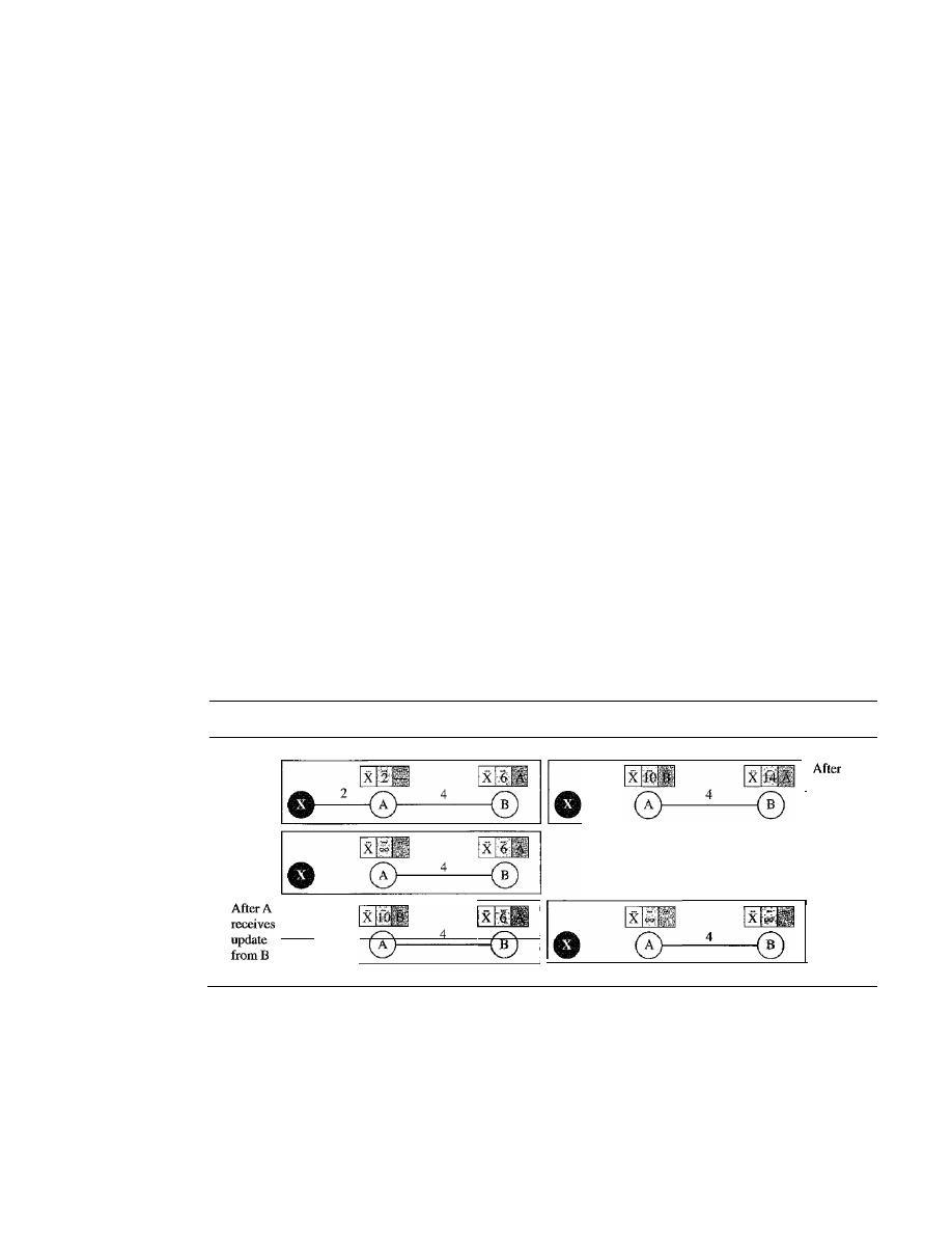
SECTION
22.3
UNICAST ROUTING PROTOCOLS
663
Each node can update its table by using the tables received from other nodes. In a
short time, if there is no change in the network itself, such as a failure in a link, each
node reaches a stable condition in which the contents of its table remains the same.
When to Share
The question now is, When does a node send its partial routing table (only two columns)
to all its immediate neighbors? The table is sent both periodically and when there is a
change in the table.
Periodic Update
A node sends its routing table, normally every 30 s, in a periodic
update. The period depends on the protocol that is using distance vector routing.
Triggered Update
A node sends its two-column routing table to its neighbors any-
time there is a change in its routing table. This is called a triggered update. The
change can result from the following.
1.
A node receives a table from a neighbor, resulting in changes in its own table after
updating.
2.
A node detects some failure in the neighboring links which results in a distance
change to infinity.
Two-Node Loop Instability
A problem with distance vector routing is instability, which means that a network using
this protocol can become unstable. To understand the problem, let us look at the scenario
depicted in Figure 22.17.
Figure 22.17
Two-node instability
Before
failure
After
failure
·
•
·
I
B
receives
update
from A
I_o
____
4__
Finally
Figure 22.17 shows a system with three nodes. We have shown only the portions of
the routing table needed for our discussion. At the beginning, both nodes A and B know
how to reach node X. But suddenly, the link between A and X fails. Node A changes its
table.
If
A can send its table to B immediately, everything is fine. However, the system
becomes unstable if B sends its routing table to A before receiving A's routing table.
Node A receives the update and, assuming that B has found a way to reach X, immedi-
ately updates its routing table. Based on the triggered update strategy, A sends its new

664
CHAPTER
22
NETWORK LAYER: DELIVERY, FORWARDING, AND ROUTING
update to B. Now B thinks that something has been changed around A and updates its
routing table. The cost of reaching X increases gradually until it reaches infinity. At this
moment, both A and B know that X cannot be reached. However, during this time the
system is not stable. Node A thinks that the route to X is via B; node B thinks that the
route to X is via A. If A receives a packet destined for X, it goes to B and then comes
back to A. Similarly, if B receives a packet destined for X, it goes to A and comes back
to
Packets bounce between A and B, creating a two-node loop problem. A few solu-
tions have been proposed for instability of this kind.
Defining Infinity
The first obvious solution is to redefine infinity to a smaller num-
ber, such as 100. For our previous scenario, the system will be stable in less than 20
updates. As a matter of fact, most implementations of the distance vector protocol
define the distance between each node to be I and define 16 as infinity. However, this
means that the distance vector routing cannot be used in large systems. The size of the
network, in each direction, can not exceed 15 hops.
Split Horizon
Another solution is called split horizon. In this strategy, instead of
flooding the table through each interface, each node sends only part of its table through
each interface. If, according to its table, node B thinks that the optimum route to reach
X is via A,
it
does not need to advertise this piece of information to A; the information
has corne from A (A already knows). Taking information from node A, modifying it,
and sending it back to node A creates the confusion. In our scenario, node B eliminates
the last line of its routing table before it sends it to A. In this case, node A keeps the
value of infinity as the distance to X. Later when node A sends its routing table to B,
node B also corrects its routing table. The system becomes stable after the first update:
both node A and B know that X is not reachable.
Split Horizon and Poison Reverse
Using the split horizon strategy has one draw-
back. Normally, the distance vector protocol uses a timer, and if there is no news about
a route, the node deletes the route from its table. When node B in the previous scenario
eliminates the route to X from its advertisement to A, node A cannot guess that this is
due to the split horizon strategy (the source of information was A) or because B has not
received any news about X recently. The split horizon strategy can be combined with
the poison reverse strategy. Node B can still advertise the value for X, but if the source
of information is A, it can replace the distance with infinity as a warning: "Do not use
this value; what I know about this route comes from you."
Three-Node Instability
The two-node instability can be avoided by using the split horizon strategy combined
with poison reverse. However, if the instability is between three nodes, stability cannot
be guaranteed. Figure 22.18 shows the scenario.
Suppose, after finding that X is not reachable, node A sends a packet to Band C to
inform them of the situation. Node B immediately updates its table, but the packet to C
is lost in the network and never reaches
Node C remains in the dark and still thinks
that there is a route to X via A with a distance of 5. After a while, node C sends to Bits
routing table, which includes the route to X. Node B is totally fooled here.
It
receives
information on the route to X from C, and according to the algorithm,
it
updates its
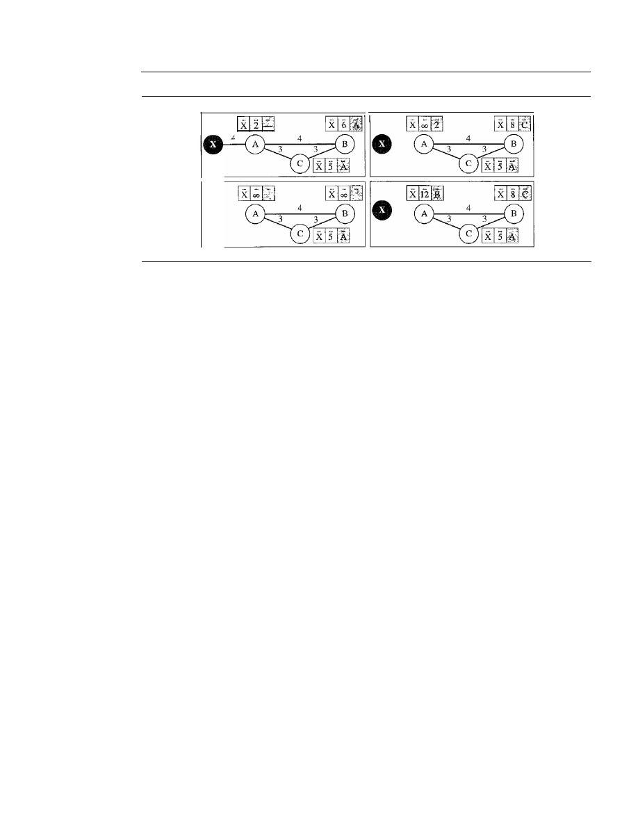
SECTION
22.3
UNICAST ROUTING PROTOCOLS
665
Figure 22.18
Three-node instability
Before failure
After A sends
the route to
B
0
and C,
but the
packet to C
is lost
2
After B sends
the route to A
After C sends
the route to B
table, showing the route to X via C with a cost of 8. This information has come from C,
not from A, so after awhile node B may advertise this route to A. Now A is fooled and
updates its table to show that A can reach X via B with a cost of 12. Of course, the loop
continues; now A advertises the route to X to C, with increased cost, but not to B. Node
C then advertises the route to B with an increased cost. Node B does the same to A.
And so on. The loop stops when the cost in each node reaches infinity.
RIP
The Routing Information Protocol (RIP) is an intradomain routing protocol used
inside an autonomous system. It is a very simple protocol based on distance vector
routing. RIP implements distance vector routing directly with some considerations:
1. In an autonomous system, we are dealing with routers and networks (links). The
routers have routing tables; networks do not.
2. The destination in a routing table is a network, which means the first column
defines a network address.
3. The metric used by RIP is very simple; the distance is defined as the number of
links (networks) to reach the destination. For this reason, the metric in RIP is called
a hop count.
4. Infinity is defined as 16, which means that any route in an autonomous system using
RIP cannot have more than 15 hops.
5. The next-node column defines the address of the router to which the packet is to be
sent to reach its destination.
Figure 22.19 shows an autonomous system with seven networks and four routers. The
table of each router is also shown. Let us look at the routing table for Rl. The table has
seven entries to show how to reach each network in the autonomous system. Router Rl is
directly connected to networks 130.10.0.0 and 130.11.0.0, which means that there are no
next-hop entries for these two networks. To send a packet to one of the three networks at
the far left, router Rl needs to deliver the packet to R2. The next-node entry for these
three networks is the interface of router R2 with IP address 130.10.0.1. To send a packet
to the two networks at the far right, router Rl needs to send the packet to the interface of
router R4 with IP address 130.11.0.1. The other tables can be explained similarly.
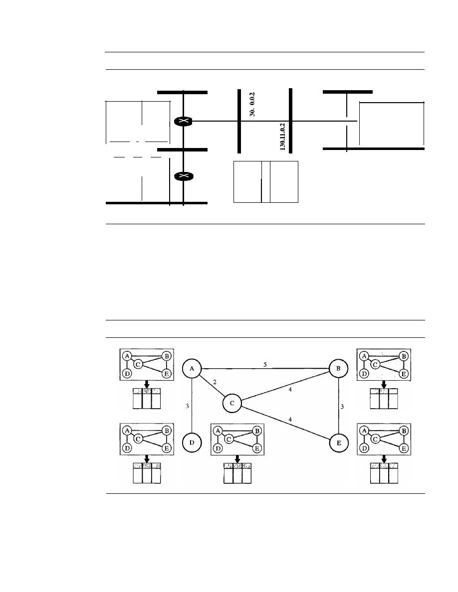
666
CHAPTER
22
NETWORK LAYER: DELIVERY, FORWARDING, AND ROUTING
Figure 22.19
Example of a domain using RIP
195.2.4.0
130.10.0.0
130.11.0.0
205.5.5.0
Dest.
Hop
Next
130.10.0.0 2
130.11.0.2
130.11.0.0
1
195.2.4.0
3
130.11.0.2
195.2.5.0
3
130.11.0.2
195.2.6.0
4
130.11.0.2
205.5.5.0
1
205.5.6.0
1
R4 Table
205.5.6.0
205.5.5.1
R4
130.11.0.1
205.5.6.1
RI Table
...
R1
...
Des!
Hop
Next
130.10.0.0
1
- -
130.11.0.0
1
- -
195.2.4.0
2
130.10.0.1
195.2.5.0
2
130.10.0.1
195.2.6.0
3
130.10.0.1
205.5.5.0
2
130.11.0.1
205.5.6.0
2
130.11.0.1
130.10.0.1
195.2.5.1
195.2.5.0
195.2.5.2
195.2.4.1
R3
195.2.6.1
195.2.6.0
Dest.
Hop
Next
R3 Table
130.10.0.0
1
130.11.0.0
2
130.10.0.2
195.2.4.0
1
195.2.5.0
1
195.2.6.0
2
195.2.5.2
R2
205.5.5.0
3
130.10.0.2
205.5.6.0
3
130.10.0.2
R2 Table
Dest.
Hop
Next
130.10.0.0
2
195.2.5.1
130.11.0.0
3
195.2.5.1
195.2.4.0
2
195.2.5.1
195.2.5.0
1
195.2.6.0
1
205.5.5.0
4
195.2.5.1
205.5.6.0
4
195.2.5.1
Link State Routing
Link state routing has a different philosophy from that of distance vector routing. In
link state routing, if each node in the domain has the entire topology of the domain-
the list of nodes and links, how they are connected including the type, cost (metric), and
condition of the links (up or down)-the node can use Dijkstra's algorithm to build a
routing table. Figure 22.20 shows the concept.
Figure 22.20
Concept of link state routing
The figure shows a simple domain with five nodes. Each node uses the same topology
to create a routing table, but the routing table for each node is unique because the calcu-
lations are based on different interpretations of the topology. This is analogous to a city
map. While each person may have the same map, each needs to take a different route to
reach her specific destination.
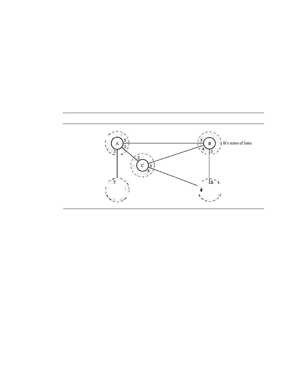
SECTION
22.3
UNICAST ROUTING PROTOCOLS
667
The topology must be dynamic, representing the latest state of each node and each
link.
If
there are changes in any point in the network (a link is down, for example), the
topology must be updated for each node.
How can a common topology be dynamic and stored in each node? No node can
know the topology at the beginning or after a change somewhere in the network. Link
state routing is based on the assumption that, although the global knowledge about the
topology is not clear, each node has partial knowledge: it knows the state (type, condi-
tion, and cost) of its links.
In
other words, the whole topology can be compiled from the
partial knowledge of each node. Figure 22.21 shows the same domain as in Figure 22.20,
indicating the part of the knowledge belonging to each node.
Figure 22.21
Link state knowledge
I
A's states of links
I
D's states of links
I
C's states ofIinks
I
I
\
t
I
E's states ofIinks
Node A knows that it is connected to node B with metric 5, to node C with metric 2,
and to node D with metric 3. Node C knows that it is connected to node A with metric 2,
to node B with metric 4, and to node E with metric 4. Node D knows that it is con-
nected only to node A with metric 3. And so on. Although there is an overlap in the
knowledge, the overlap guarantees the creation of a common topology-a picture of
the whole domain for each node.
Building Routing Tables
In link state routing,
four sets of actions are required to ensure that each node has the
routing table showing the least-cost node to every other node.
]. Creation of the states of the links by each node, called the link state packet (LSP).
2. Dissemination of LSPs to every other router, called
flooding,
in an efficient and
reliable way.
3. Formation of a shortest path tree for each node.
4. Calculation of a routing table based on the shortest path tree.
Creation of Link State Packet (LSP)
A link state packet can carry a large amount
of information. For the moment, however, we assume that it carries a minimum amount

668
CHAPTER
22
NETWORK LAYER: DELIVERY, FORWARDING, AND ROUTING
of data: the node identity, the list of links, a sequence number, and age. The first two,
node identity and the list of links, are needed to make the topology. The third, sequence
number, facilitates flooding and distinguishes new LSPs from old ones. The fourth, age,
prevents old LSPs from remaining in the domain for a long time. LSPs are generated on
two occasions:
1. When there is a change in the topology of the domain.
Triggering of LSP dissemi-
nation is the main way of quickly informing any node in the domain to update its
topology.
2. On a periodic basis.
The period in this case is much longer compared to distance
vector routing. As a matter of fact, there is no actual need for this type of LSP dis-
semination. It is done to ensure that old information is removed from the domain.
The timer set for periodic dissemination is normally in the range of 60 min or 2 h
based on the implementation. A longer period ensures that flooding does not create
too much traffic on the network.
Flooding of LSPs
After a node has prepared an LSP, it must be disseminated to all
other nodes, not only to its neighbors. The process is called flooding and based on the
following:
1. The creating node sends a copy of the LSP out of each interface.
2. A node that receives an LSP compares it with the copy it may already have.
If
the
newly arrived LSP is older than the one it has (found by checking the sequence
number), it discards the LSP.
If
it is newer, the node does the following:
a.
It
discards the old LSP and keeps the new one.
b.
It
sends a copy of it out of each interface except the one from which the packet
arrived. This guarantees that flooding stops somewhere in the domain (where a
node has only one interface).
Formation of Shortest Path Tree: Dijkstra Algorithm
After receiving all LSPs, each
node will have a copy of the whole topology. However, the topology is not sufficient to
find the shortest path to every other node; a shortest path tree is needed.
A tree is a graph of nodes and links; one node is called the root. All other nodes
can be reached from the root through only one single route. A shortest path tree is a tree
in which the path between the root and every other node is the shortest. What we need
for each node is a shortest path tree with that node as the root.
The Dijkstra algorithm creates a shortest path tree from a graph. The algorithm
divides the nodes into two sets: tentative and permanent.
It
finds the neighbors of a
current node, makes them tentative, examines them, and if they pass the criteria,
makes them permanent. We can informally define the algorithm by using the flowchart
in Figure 22.22.
Let us apply the algorithm to node A of our sample graph in Figure 22.23. To find
the shortest path in each step, we need the cumulative cost from the root to each node,
which is shown next to the node.
The following shows the steps. At the end of each step, we show the permanent
(filled circles) and the tentative (open circles) nodes and lists with the cumulative
costs.
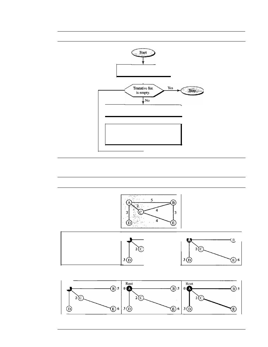
SECT/ON
22.3
UN/CAST ROUTING PROTOCOLS
669
Figure 22.22
Dijkstra algorithm
Set root to local node and
move it to tentative list.
Among nodes in tentative list, move the
one with the shortest path to permanent list.
Add each unprocessed neighbor of last moved
node to tentative list if not already there.
If neighbor is in the tentative list with larger
cumulative cost, replace it with new one.
Figure 22.23
Example offormation of shortest path tree
Root
B 5
0
5
Root
00
I. Set root to A and move A to
tentative list.
Root
o .
3
4. Move D to permanent list.
Root
o .
2. Move A to permanent list and
add
B, C, and D to tentative list.
5. Move B to permanent list.
Topology
3. Move C to permanent and add
E to tentative list.
6
6. Move E to permanent list
(tentative list is empty).

670
CHAPTER 22
NETWORK LAYER: DELIVERY, FORWARDING, AND ROUTING
1. We make node A the root of the tree and move it to the tentative list. Our two lists are
Permanent list: empty
Tentative list: A(O)
2. Node A has the shortest cumulative cost from all nodes in the tentative list. We move A
to the pennanent list and add all neighbors of A to the tentative list. Our new lists
are
Permanent list: A(O)
Tentative list:
B(5),
D(3)
3. Node C has the shortest cumulative cost from all nodes in the tentative list. We move
C
to the permanent list. Node
C
has three neighbors, but node
A
is already pro-
cessed, which makes the unprocessed neighbors just B and E. However, B is already
in the tentative list with a cumulative cost of
5.
Node
A
could also reach node
B
through C with a cumulative cost of 6. Since 5 is less than 6, we keep node B with a
cumulative cost of
5
in the tentative list and do not replace it. Our new lists are
Permanent list: A(O),
e(2)
Tentative
list:
0(3), E(6)
4. Node D has the shortest cumulative cost of all the nodes in the tentative list. We
move D to the permanent list. Node D has no unprocessed neighbor to be added to
the tentative list. Our new lists are
Permanent list: A(O),
C(2), 0(3)
Tentative list:
B(5), E(6)
5. Node B has the shortest cumulative cost of all the nodes in the tentative list. We
move B to the permanent list. We need to add all unprocessed neighbors of B to the
tentative list (this is just node E). However, E(6) is already in the list with a smaller
cumulative cost. The cumulative cost to node E, as the neighbor of B, is 8. We keep
node E(6) in the tentative list. Our new lists are
Permanent list: A(O),
B(5), C(2), 0(3)
Tentative list: E(6)
6. Node E has the shortest cumulative cost from all nodes in the tentative list. We
move E to the permanent list. Node E has no neighbor. Now the tentative list is
empty. We stop; our shortest path tree is ready. The final lists are
Permanent list:
B(5), C(2),
E(6)
Tentative list: empty
Calculation of Routing Table from Shortest Path Tree
Each node uses the short-
est path tree protocol to construct its routing table. The routing table shows the cost of
reaching each node from the root. Table 22.2 shows the routing table for node A.
Table 22.2
Routing table for node A
Node
Cost
Next Router
A
0
-
B
5
-
C
2
-
D
3
-
E
6
C
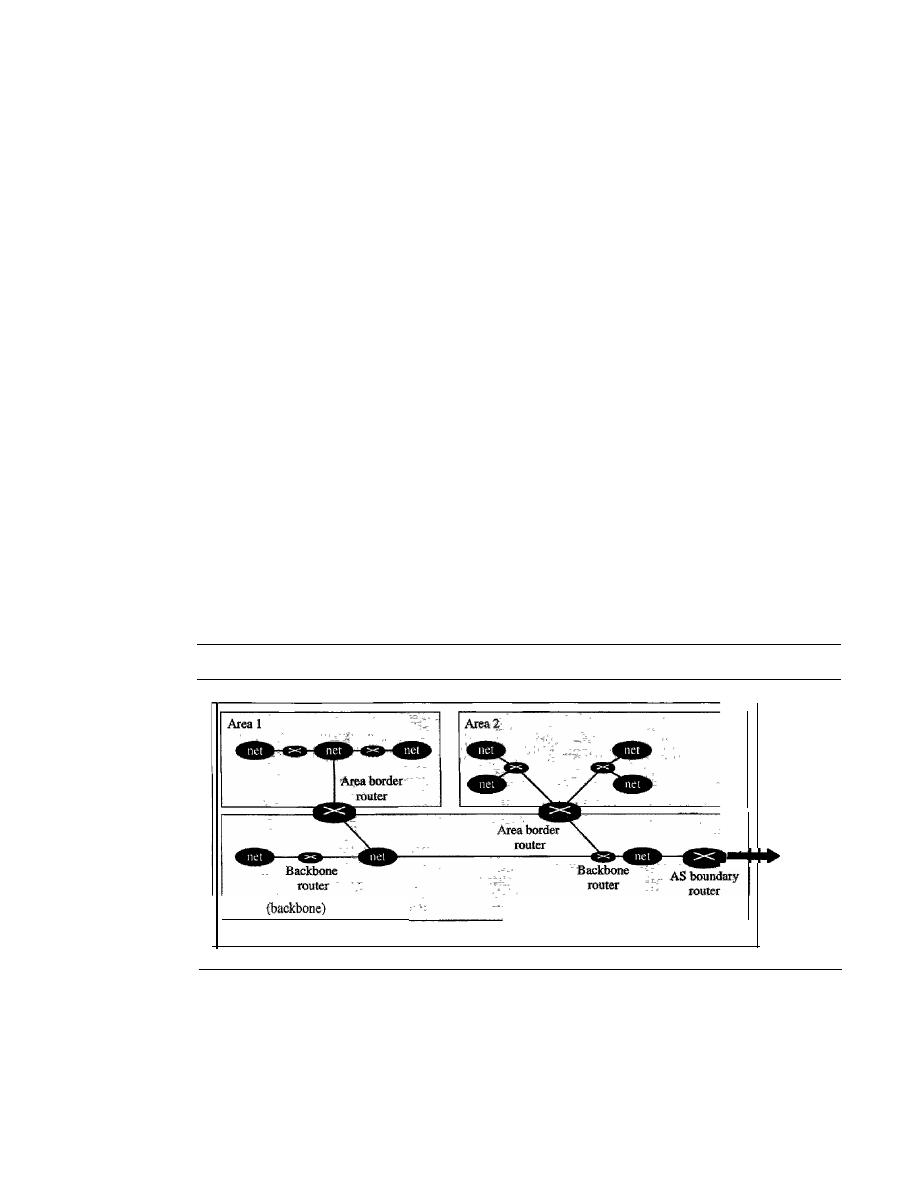
SECTION
22.3
UN/CAST ROUTING PROTOCOLS
671
Compare Table 22.2 with the one in Figure 22.14. Both distance vector routing and
link
state routing end up with the same routing table for node
A.
OSPF
The Open Shortest Path First or
OSPF protocol is an intradomain routing protocol
based on link state routing. Its domain is also an autonomous system.
Areas
To handle routing efficiently and in a timely manner, OSPF divides an auto-
nomous system into areas. An
area is a collection of networks, hosts, and routers all
contained within an autonomous system. An autonomous system can be divided into
many different areas. All networks inside an area must be connected.
Routers inside an area flood the area with routing information. At the border of an
area, special routers called
area border routers summarize the information about the
area and send it to other areas. Among the areas inside an autonomous system is a spe-
cial area called the
backbone;
all the areas inside an autonomous system must be con-
nected to the backbone. In other words, the backbone serves as a primary area and the
other areas as secondary areas. This does not mean that the routers within areas cannot
be connected to each other, however. The routers inside the backbone are called the
backbone routers. Note that a backbone router can also be an area border router.
If,
because of some problem, the connectivity between a backbone and an area is
broken, a
virtual link between routers must be created by an administrator to allow
continuity of the functions of the backbone as the primary area.
Each area has an area identification. The area identification of the backbone is
zero. Figure 22.24 shows an autonomous system and its areas.
Figure 22.24
Areas in an autonomous system
Area
0
To other
ASs
Autonomous system
Metric
The OSPF protocol allows the administrator to assign a cost, called the
metric,
to each route. The metric can be based on a type of service (minimum delay, maximum
throughput, and so on). As a matter of fact, a router can have multiple routing tables,
each based on a different type of service.
Types of Links
In OSPF terminology, a connection is called a
link.
Four types of
links have been defined: point-to-point, transient, stub, and virtual (see Figure 22.25).
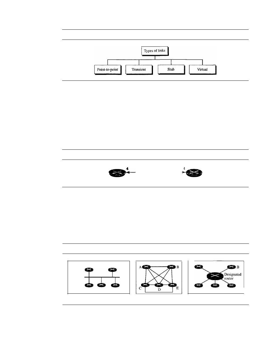
672
CHAPTER
22
NETWORK LAYER: DELIVERY, FORWARDING, AND ROUTING
Figure 22.25
Types of links
A point-to-point link connects two routers without any other host or router in
between. In other words, the purpose of the link (network) is just to connect the two
routers. An example of this type of link is two routers connected by a telephone line or
a T line. There is no need to assign a network address to this type of link. Graphically,
the routers are represented by nodes, and the link is represented by a bidirectional edge
connecting the nodes. The metrics, which are usually the same, are shown at the two
ends, one for each direction. In other words, each router has only one neighbor at the
other side of the link (see Figure 22.26).
Figure 22.26
Point-to-point link
Point-to-point network
Router
Router
A transient link is a network with several routers attached to it. The data can enter
through any of the routers and leave through any router. All LANs and some WANs with
two or more routers are of this type. In this case, each router has many neighbors. For
example, consider the Ethernet in Figure 22.27a. Router A has routers B, C, D, and E as
neighbors. Router B has routers A, C, D, and E as neighbors.
If
we want to show the
neighborhood relationship in this situation, we have the graph shown in Figure 22.27b.
Figure 22.27
Transient link
A
E
D
c
A
b. Unrealistic representation
c. Realistic representation
E
B
D
c
Ethernet
a. Transient network
This is neither efficient nor realistic.
It
is not efficient because each router needs to
advertise the neighborhood to four other routers, for a total of 20 advertisements.
It
is
SECTION
22.3
UNICAST ROUTING PROTOCOLS
673
not realistic because there is no single network (link) between each pair of routers;
there is only one network that serves as a crossroad between all five routers.
To show that each router is connected to every other router through one single net-
work, the network itself is represented by a node. However, because a network is not a
machine, it cannot function as a router. One of the routers in the network takes this
responsibility.
It
is assigned a dual purpose; it is a true router and a designated router.
We can use the topology shown in Figure 22.27c to show the connections of a transient
network.
Now each router has only one neighbor, the designated router (network). On the
other hand, the designated router (the network) has five neighbors. We see that thc
number of neighbor announcements is reduced from 20 to 10. Still, the link is repre-
sented as a bidirectional edge between the nodes. However, while there is a metric from
each node to the designated router, there is no metric from the designated router to any
other node. The reason is that the designated router represents the network. We can
only assign a cost to a packet that is passing through the network. We cannot charge for
this twice. When a packet enters a network, we assign a cost; when a packet leaves the
network to go to the router, there is no charge.
A stub link is a network that is connected to only one router. The data packets
enter the network through this single router and leave the network through this same
router. This is a special case of the transient network. We can show this situation using
the router as a node and using the designated router for the network. However, the link
is only one-directional, from the router to the network (see Figure 22.28).
Figure 22.28
Stub link
A
Ethernet
a. Stub network
A
...
b. Representation
When the link between two routers is broken, the administration may create a
virtual link between them, using a longer path that probably goes through several
routers.
Graphical Representation
Let us now examine how an AS can be represented
graphically. Figure 22.29 shows a small AS with seven networks and six routers. Two
of the networks are point-to-point networks. We use symbols such as Nl and N2
for transient and stub networks. There is no need to assign an identity to a point-to-
point network. The figure also shows the graphical representation of the AS as seen
by OSPF.
We have used square nodes for the routers and ovals for the networks (represented
by designated routers). However, OSPF sees both as nodes. Note that we have three
stub networks.
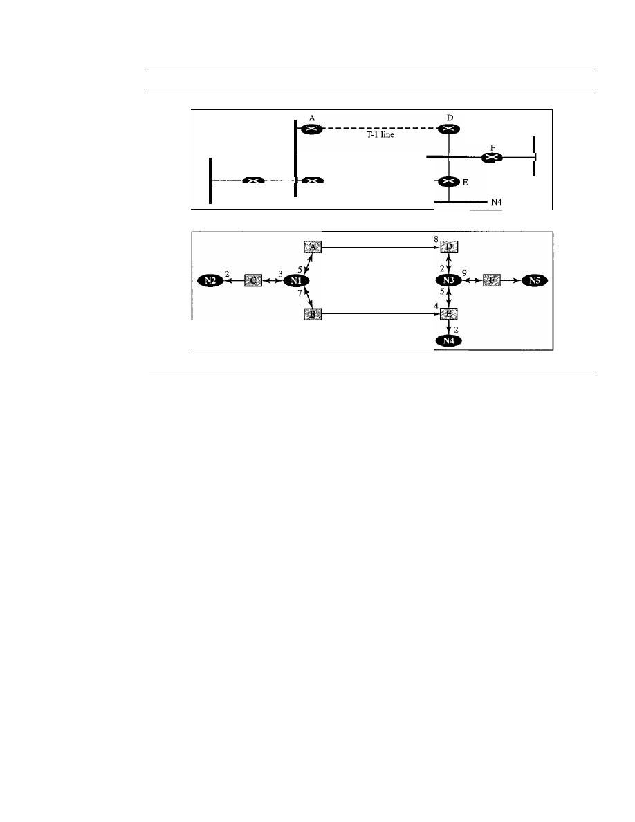
674
CHAPTER
22
NETWORK LAYER: DELIVERY, FORWARDING, AND ROUTING
Figure 22.29
Example of an AS and its graphical representation in OSPF
- - - - - - - - - - - - - -
N2
c
Nl
a. Autonomous system
B
T-31ine
N3
N5
b. Graphical representation
8
4
Path Vector Routing
Distance vector and link state routing are both intradomain routing protocols. They can
be used inside an autonomous system, but not between autonomous systems. These two
protocols are not suitable for interdomain routing mostly because of scalability. Both of
these routing protocols become intractable when the domain of operation becomes
large. Distance vector routing is subject to instability if there are more than a few hops
in the domain of operation. Link state routing needs a huge amount of resources to cal-
culate routing tables.
It
also creates heavy traffic because of flooding. There is a need
for a third routing protocol which we call
path vector routing.
Path vector routing proved to be useful for interdomain routing. The principle of
path vector routing is similar to that of distance vector routing. In path vector routing,
we assume that there is one node (there can be more, but one is enough for our concep-
tual discussion) in each autonomous system that acts on behalf of the entire autono-
mous system. Let us call it the
speaker node. The speaker node in an AS creates a
routing table and advertises it to speaker nodes in the neighboring ASs. The idea is the
same as for distance vector routing except that only speaker nodes in each AS can com-
municate with each other. However, what is advertised is different. A speaker node
advertises the path, not the metric of the nodes, in its autonomous system or other
autonomous systems.
Initialization
At the beginning, each speaker node can know only the reachability of nodes inside its
autonomous system. Figure 22.30 shows the initial tables for each speaker node in a
system made of four ASs.
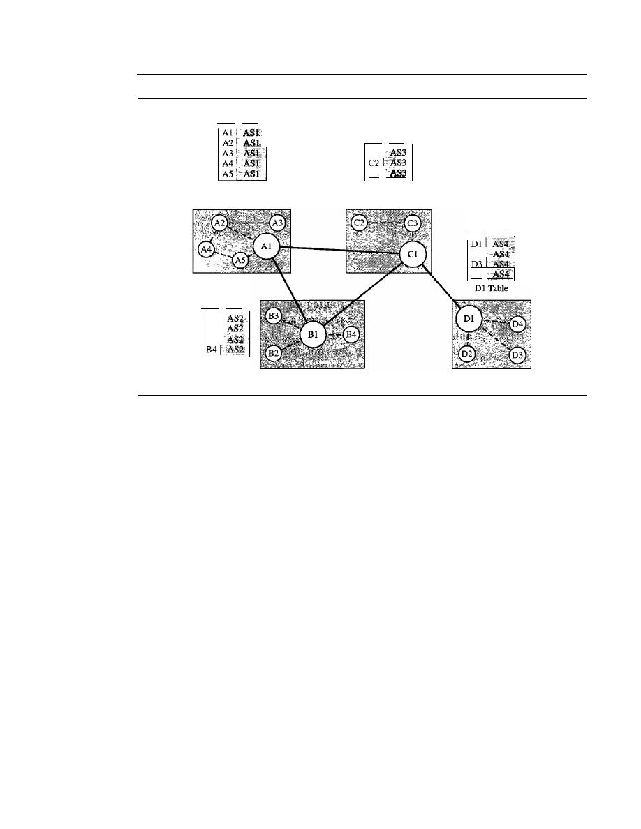
SECTION
22.3
UNICAST ROUTING PROTOCOLS
675
Figure 22.30
Initial routing tables in path vector routing
Dest. Path
Al Table
AS 1
Des!. Path
Bl
B2
B3
BI Table
AS 2
Dest. Path
CI
C3
Cl Table
AS3
Des!' Path
D2
D4
AS4
Node Al is the speaker node for ASl, Bl for AS2, Cl for AS3, and Dl for AS4.
Node Al creates an initial table that shows Al to A5 are located in ASI and can be
reached through it. Node Bl advertises that Bl to B4 are located in AS2 and can be
reached through Bl. And so on.
Sharing
Just as in distance vector routing, in path vector routing, a speaker in an
autonomous system shares its table with immediate neighbors. In Figure 22.30, node
Al shares its table with nodes Bl and Cl. Node Cl shares its table with nodes Dl, Bl,
andAl. Node Bl shares its table with Cl andAl. Node Dl shares its table with Cl.
Updating
When a speaker node receives a two-column table from a neighbor, it
updates its own table by adding the nodes that are not in its routing table and adding its
own autonomous system and the autonomous system that sent the table. After a while
each speaker has a table and knows how to reach each node in other ASs. Figure 22.31
shows the tables for each speaker node after the system is stabilized.
According to the figure, if router Al receives a packet for nodes A3, it knows that
the path is in ASI (the packet is at home); but if it receives a packet for Dl, it knows that
the packet should go from ASl, to AS2, and then to AS3. The routing table shows the
path completely. On the other hand, if node Dl in AS4 receives a packet for node A2, it
knows
it
should go through AS4, AS3, and AS
1.
o
Loop prevention. The instability of distance vector routing and the creation of
loops can be avoided in path vector routing. When a router receives a message, it
checks to see if its autonomous system is in the path list to the destination.
If
it is,
looping is involved and the message is ignored.
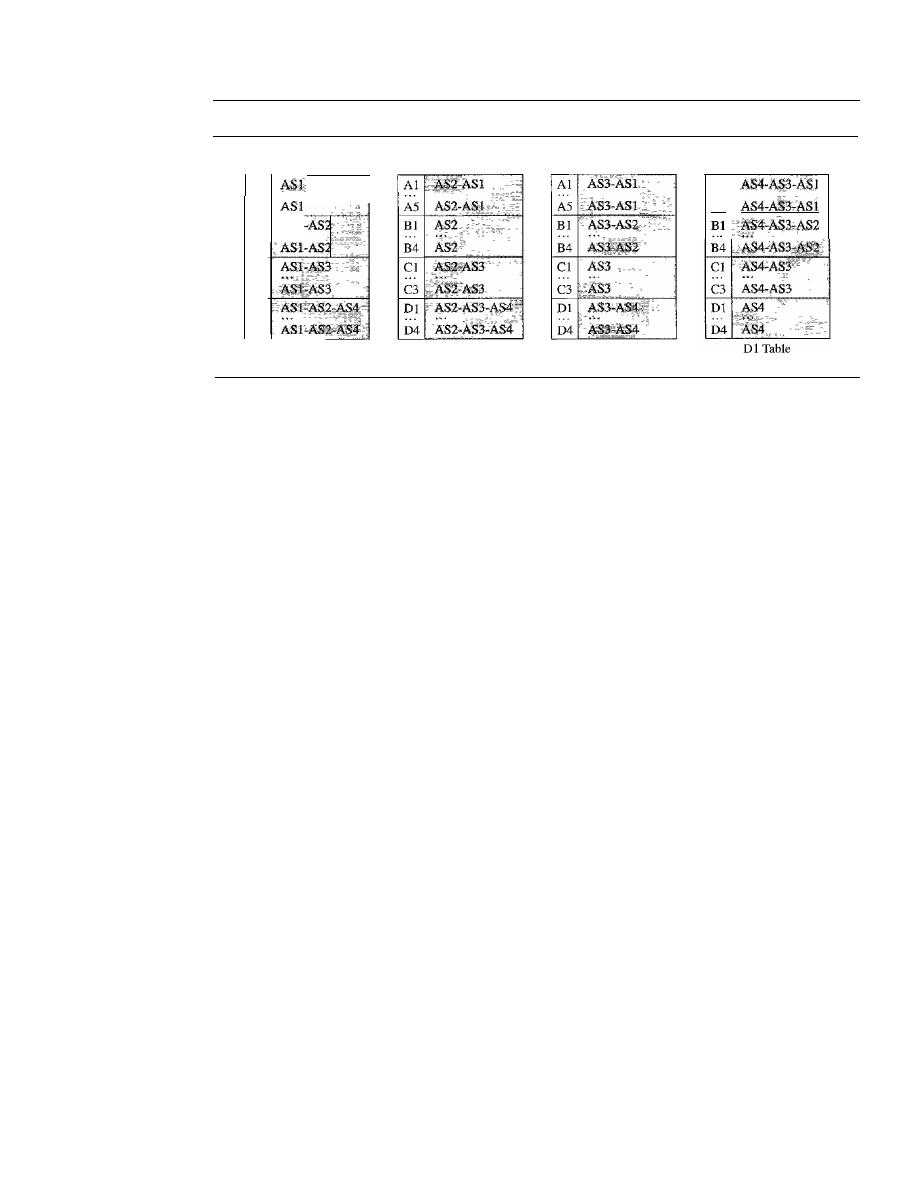
676
CHAPTER
22
NETWORK LAYER: DELIVERY, FORWARDING, AND ROUTING
Figure 22.31
Stabilized tables for three autonomous systems
Al
A5
Dest.
Path
Path
Cl Table
Oest.
Path
Bl Table
Oest.
Oest.
Path
Al
AS
Bl
B4
Cl
...
C3
01
D4
Al Table
o
Policy routing.
Policy routing can be easily implemented through path vector
routing. When a router receives a message, it can check the path.
If
one of the
autonomous systems listed in the path is against its policy, it can ignore that path
and that destination. It does not update its routing table with this path, and it does
not send this message to its neighbors.
o
Optimum path.
What is the optimum path in path vector routing? We are looking
for a path to a destination that is the best for the organization that runs the autono-
mous system. We definitely cannot include metrics in this route because each
autonomous system that is included in the path may use a different criterion for the
metric. One system may use, internally, RIP, which defines hop count as the metric;
another may use OSPF with minimum delay defined as the metric. The optimum
path is the path that fits the organization. In our previous figure, each autonomous
system may have more than one path to a destination. For example, a path from
AS4 to ASI can be AS4-AS3-AS2-AS1, or it can be AS4-AS3-ASI. For the tables,
we chose the one that had the smaller number of autonomous systems, but this is
not always the case. Other criteria, such as security, safety, and reliability, can also
be applied.
BGP
Border Gateway Protocol (BGP) is an interdomain routing protocol using path vector
routing. It first appeared in 1989 and has gone through four versions.
Types of Autonomous Systems
As we said before, the Internet is divided into hier-
archical domains called autonomous systems. For example, a large corporation that
manages its own network and has full control over it is an autonomous system. A local
ISP that provides services to local customers is an autonomous system. We can divide
autonomous systems into three categories: stub, multihomed, and transit.
o
Stub
AS. A stub AS has only one connection to another AS. The interdomain data
traffic in a stub AS can be either created or terminated in the AS. The hosts in the AS
can send data traffic to other ASs. The hosts in the AS can receive data coming from
hosts in other ASs. Data traffic, however, cannot pass through a stub AS. A stub AS

SECTION
22.3
UNICAST ROUTING PROTOCOLS
677
is either a source or a sink. A good example of a stub AS is a small corporation or a
small local ISP.
o
Multihomed AS. A multihomed AS has more than one connection to other ASs,
but it is still only a source or sink for data traffic. It can receive data traffic from
more than one AS.
It
can send data traffic to more than one AS, but there is no tran-
sient traffic. It does not allow data coming from one AS and going to another AS to
pass through. A good example of a multihomed AS is a large corporation that is con-
nected to more than one regional or national AS that does not allow transient traffic.
o
Transit AS. A transit AS is a multihomed AS that also allows transient traffic. Good
examples of transit ASs are national and international ISPs (Internet backbones).
Path Attributes
In our previous example, we discussed a path for a destination net-
work. The path was presented as a list of autonomous systems, but is, in fact, a list of
attributes. Each attribute gives some information about the path. The list of attributes
helps the receiving router make a more-informed decision when applying its policy.
Attributes are divided into two broad categories: well known and optional. A
well-
known attribute is one that every BGP router must recognize.
An
optional attribute
is one that needs not be recognized by every router.
Well-known attributes are themselves divided into two categories: mandatory and
discretionary. A
well-known mandatory attribute
is one that must appear in the descrip-
tion of a route. A
well-known discretionary attribute
is one that must be recognized by
each router, but is not required to be included in every update message. One
known mandatory attribute is ORIGIN. This defines the source of the routing informa-
tion (RIP, OSPF, and so on). Another well-known mandatory attribute is AS_PATH.
This defines the list of autonomous systems through which the destination can be
reached. Still another well-known mandatory attribute is NEXT-HOP, which defines
the next router to which the data packet should be sent.
The optional attributes can also be subdivided into two categories: transitive and
nontransitive. An
optional transitive attribute
is one that must be passed to the next
router by the router that has not implemented this attribute. An
optional nontransitive
attribute
is one that must be discarded if the receiving router has not implemented it.
BGP Sessions
The exchange of routing information between two routers using BGP
takes place in a session. A session is a connection that is established between two BGP
routers only for the sake of exchanging routing information. To create a reliable envi-
ronment, BGP uses the services of TCP. In other words, a session at the BGP level, as
an application program, is a connection at the TCP level. However, there is a subtle dif-
ference between a connection in TCP made for BGP and other application programs.
When a TCP connection is created for BGP, it can last for a long time, until something
unusual happens. For this reason, BGP sessions are sometimes referred to as
semi-
pennanent connections.
External and Internal BGP
If
we want to be precise, BGP can have two types of
sessions: external BGP (E-BGP) and internal BGP (I-BGP) sessions. The E-BGP ses-
sion is used to exchange information between two speaker nodes belonging to two dif-
ferent autonomous systems. The I-BGP session, on the other hand, is used to exchange
routing information between two routers inside an autonomous system. Figure 22.32
shows the idea.
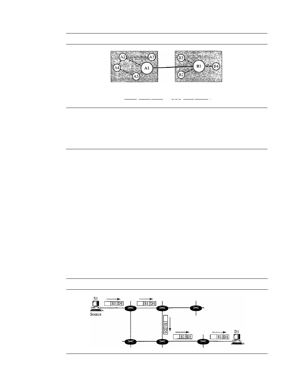
678
CHAPTER
22
NETWORK LAYER: DELIVERY, FORWARDING, AND ROUTING
Figure 22.32
Internal and external BGP sessions
AS 1
AS 2
1--
E-BGP session
- - -
I-BGP sessions
I
The session established between AS 1 and AS2 is an E-BOP session. The two speaker
routers exchange information they know about networks in the Internet. However, these
two routers need to collect information from other routers in the autonomous systems.
This is done using I-BOP sessions.
22.4
MULTICAST ROUTING PROTOCOLS
In this section, we discuss multicasting and multicast routing protocols. We first define
the term multicasting and compare it to unicasting and broadcasting. We also briefly
discuss the applications of multicasting. Finally, we move on to multicast routing and
the general ideas and goals related to it. We also discuss some common multicast routing
protocols used in the Internet today.
Unicast, Multicast,
and
Broadcast
A message can be unicast, multicast, or broadcast. Let us clarify these terms as they
relate to the Internet.
Unicasting
In unicast communication, there is one source and one destination. The relationship
between the source and the destination is one-to-one. In this type of communication,
both the source and destination addresses, in the IP datagram, are the unicast addresses
assigned to the hosts (or host interfaces, to be more exact). In Figure 22.33, a unicast
Figure 22.33
Unicasting
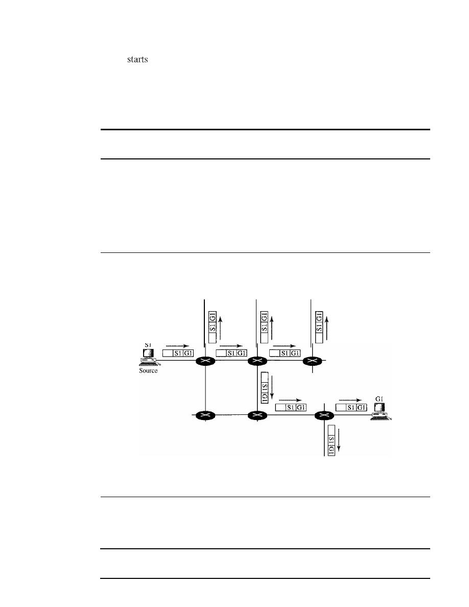
SECTION
22.4
MULTICAST ROUTING PROTOCOLS
679
packet
from the source S1 and passes through routers to reach the destination D 1.
We have shown the networks as a link between the routers to simplify the figure.
Note that in unicasting, when a router receives a packet,
it
forwards the packet
through only one of its interfaces (the one belonging to the optimum path) as defined in
the routing table. The router may discard the packet if it cannot find the destination
address in its routing table.
In unicasting, the router forwards the received packet through
only one of its interfaces.
Multicasting
In multicast communication, there is one source and a group of destinations. The rela-
tionship is one-to-many. In this type of communication, the source address is a unicast
address, but the destination address is a group address, which defines one or more desti-
nations. The group address identifies the members of the group. Figure
22.34
shows the
idea behind multicasting.
Figure 22.34
Multicasting
G1
G1
G1
Sl
GI
A multicast packet starts from the source S
1
and goes to all destinations that
belong to group G
1.
In multicasting, when a router receives a packet, it may forward it
through several of its interfaces.
In
multicasting, the router may forward the received packet
through several of its interfaces.
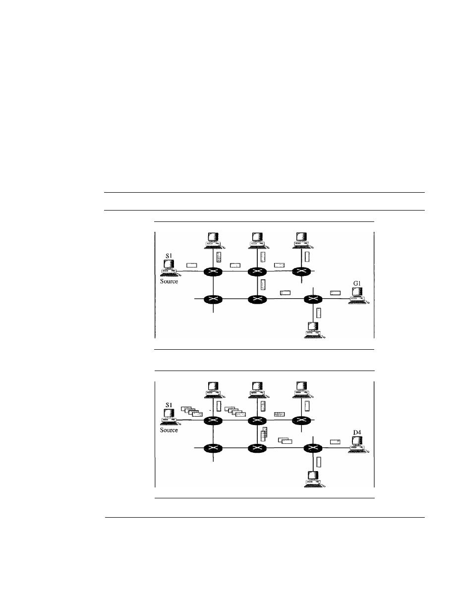
680
CHAPTER 22
NETWORK LAYER: DELIVERY, FORWARDING, AND ROUTING
Broadcasting
In broadcast communication, the relationship between the source and the destination is
one-to-all. There is only one source, but all the other hosts are the destinations. The
Internet does not explicitly support
broadcasting because of the huge amount of traffic
it would create and because of the bandwidth it would need. Imagine the traffic gener-
ated in the Internet if one person wanted to send a message to everyone else connected
to the Internet.
Multicasting Versus Multiple Unicasting
Before we finish this section, we need to distinguish between multicasting and multiple
unicasting. Figure 22.35 illustrates both concepts.
Figure 22.35
Multicasting versus multiple unicasting
Gl
Gl
Gl
Gl
a. Multicasting
Dl
D2
D3
D5
b. Multiple nnicasting
Multicasting starts with one single packet from the source that is duplicated by the
routers. The destination address in each packet is the same for all duplicates. Note that
only one single copy of the packet travels between any two routers.

SECTION
22.4
MULTICAST ROUTING PROTOCOLS
681
In
multiple unicasting,
several packets start from the source.
If
there are five
destinations, for example, the source sends five packets, each with a different unicast
destination address. Note that there may be multiple copies traveling between two routers.
For example, when a person sends an e-mail message to a group of people, this is
multiple unicasting. The e-mail software creates replicas of the message, each with a
different destination address and sends them one by one. This is not multicasting; it is
multiple unicasting.
Emulation of Multicasting with Unicasting
You might wonder why we have a separate mechanism for multicasting, when it can be
emulated with unicasting. There are two obvious reasons for this.
1. Multicasting is more efficient than multiple unicasting. In Figure 22.35, we can see
how multicasting requires less bandwidth than does multiple unicasting. In multi-
ple unicasting, some of the links must handle several copies.
2. In multiple unicasting, the packets are created by the source with a relative delay
between packets.
If
there are 1000 destinations, the delay between the first and the
last packet may be unacceptable. In multicasting, there is no delay because only
one packet is created by the source.
Emulation of multicasting through multiple unicasting is not efficient
and may create long delays, particularly with a large group.
Applications
Multicasting has many applications today such as access to
distributed databases,
information dissemination, teleconferencing, and distance learning.
Access to Distributed Databases
Most of the large databases today are distributed. That is, the information is stored in
more than one location, usually at the time of production. The user who needs to access
the database does not know the location of the information. A user's request is multi-
cast to all the database locations, and the location that has the information responds.
Information Dissemination
Businesses often need to send information to their customers.
If
the nature of the infor-
mation is the same for each customer, it can be multicast. In this way a business can
send one message that can reach many customers. For example, a software update can
be sent to all purchasers of a particular software package.
Dissemination of News
In a similar manner news can be easily disseminated through multicasting. One single
message can be sent to those interested in a particular topic. For example, the statistics
of the championship high school basketball tournament can be sent to the sports editors
of many newspapers.

682
CHAPTER 22
NETWORK LAYER: DELNERY, FORWARDING, AND ROUTING
Teleconferencing
Teleconferencing involves multicasting. The individuals attending a teleconference all
need to receive the same information at the same time. Temporary or permanent groups
can be formed for this purpose. For example, an engineering group that holds meetings
every Monday morning could have a permanent group while the group that plans the
holiday party could form a temporary group.
Distance Learning
One growing area in the use of multicasting is distance learning. Lessons taught by
one single professor can be received by a specific group of students. This is especially
convenient for those students who find it difficult to attend classes on campus.
Multicast Routing
In this section, we first discuss the idea of optimal routing, common in all multicast
protocols. We then give an overview of multicast routing protocols.
Optimal Routing: Shortest Path Trees
The process of optimal interdomain routing eventually results in the finding of the
shortest path tree.
The root of the tree is the source, and the leaves are the potential des-
tinations. The path from the root to each destination is the shortest path. However, the
number of trees and the formation of the trees in unicast and multicast routing are dif-
ferent. Let us discuss each separately.
Unicast Routing
In unicast routing, when a router receives a packet to forward, it
needs to find the shortest path to the destination of the packet. The router consults its
routing table for that particular destination. The next-hop entry corresponding to the
destination is the start of the shortest path. The router knows the shortest path for
each destination, which means that the router has a shortest path tree to optimally
reach all destinations. In other words, each line of the routing table is a shortest path;
the whole routing table is a shortest path tree. In unicast routing, each router needs
only one shortest path tree to forward a packet; however, each router has its own
shortest path tree. Figure 22.36 shows the situation.
The figure shows the details of the routing table and the shortest path tree for
router Rl. Each line in the routing table corresponds to one path from the root to the
corresponding network. The whole table represents the shortest path tree.
In unicast routing, each router in the domain has a table that defines
a shortest path tree to possible destinations.
Multicast Routing
When a router receives a multicast packet, the situation is different
from when it receives a unicast packet. A multicast packet may have destinations in more
than one network. Forwarding of a single packet to members of a group requires a
shortest path tree. If we have n groups, we may need n shortest path trees. We can imagine
the complexity of multicast routing. Two approaches have been used to solve the problem:
source-based trees and group-shared trees.
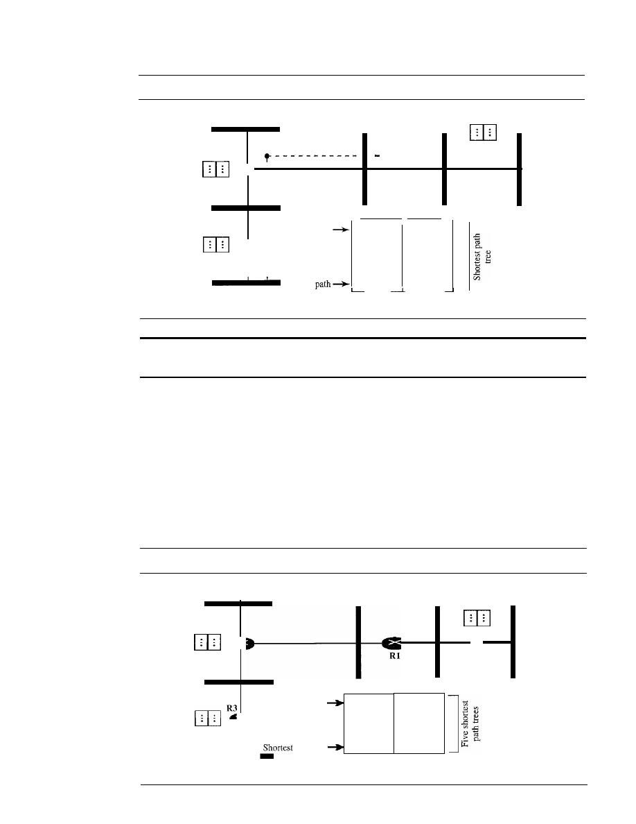
SECTION
22.4
MULTICAST ROUTING PROTOCOLS
683
Figure 22.36
Shortest path tree in unicast routing
N2
R2
R2 Table
I
I
NI
Root
--e- ---
RI
N5
R4 Table
R4
N6
R2
R2
RZ
R4
Destination Next-hop
NI
N2
N3
N4
N5
N6
Shortest path
Shortest
N4
_ _
N3
R3
R3 Table
Rl Table
In
multicast routing, each involved router needs to construct
a shortest path tree for each group.
o
Source-Based Tree. In the source-based tree approach, each router needs to have
one shortest path tree for each group. The shortest path tree for a group defines the
next hop for each network that has loyal member(s) for that group. In Figure 22.37,
we assume that we have only five groups in the domain: GI, G2, G3, G4, and G5.
At the moment G I has loyal members in four networks, G2 in three, G3 in two, G4
in two, and G5 in two. We have shown the names of the groups with loyal mem-
bers on each network. Figure 22.37 also shows the multicast routing table for
router RI. There is one shortest path tree for each group; therefore there are five
shortest path trees for five groups. If router Rl receives a packet with destination
Figure 22.37
Source-based tree approach
GI,G2
RZ
R2 Table
GI, G2
G3
Gl,G4,G5
R4 Table
R4
_ _ _ _
path tree
Rl Table
Gl
-,RZ,R4
G2
-,RZ
G3
-,RZ
G4
RZ,R4
G5
RZ,R4
Next hop
Destination
··
·
Shortest path tree
Gl,G2,G4
G3,G5
R3Table
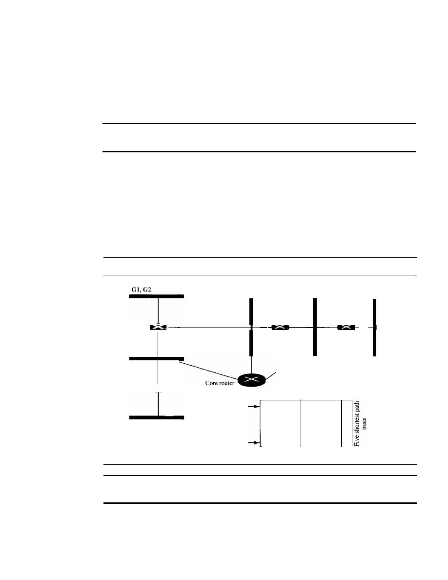
684
CHAPTER
22
NETWORK IAYER: DELIVERY, FORWARDING, AND ROUTING
address G1, it needs to send a copy of the packet to the attached network, a copy to
router R2, and a copy to router R4 so that all members of G1 can receive a copy. In
this approach, if the number of groups is
m, each router needs to have m shortest
path trees, one for each group. We can imagine the complexity of the routing table
if we have hundreds or thousands of groups. However, we will show how different
protocols manage to alleviate the situation.
In the source-based tree approach, each router needs
to have one shortest path tree for each group.
o
Group-Shared Tree.
In the
group-shared tree
approach, instead of each router
having
m shortest path trees, only one designated router, called the center core, or
rendezvous router,
takes the responsibility of distributing multicast traffic. The core
has
m shortest path trees in its routing table. The rest of the routers in the domain have
none. If a router receives a multicast packet, it encapsulates the packet in a unicast
packet and sends it to the core router. The core router removes the multicast packet
from its capsule, and consults its routing table to route the packet. Figure 22.38 shows
the idea.
Figure 22.38
Group-shared tree approach
Gl,G2
G3
Gl,G4, GS
R2
-
G3,GS
R3
Rl
R4
Gl, G2, G4
Shortest path tree
Shortest path tree
Destination
Next hop
Gl
- , R2, R3, R4
G2
-,R2,R3
G3
G4
R3,R4
G5
-,R4
Core router table
In
the group-shared tree approach, only the core router,
which has a shortest path tree for each group, is involved in multicasting.
Routing Protocols
During the last few decades, several multicast routing protocols have emerged. Some of
these protocols are extensions of unicast routing protocols; others are totally new.
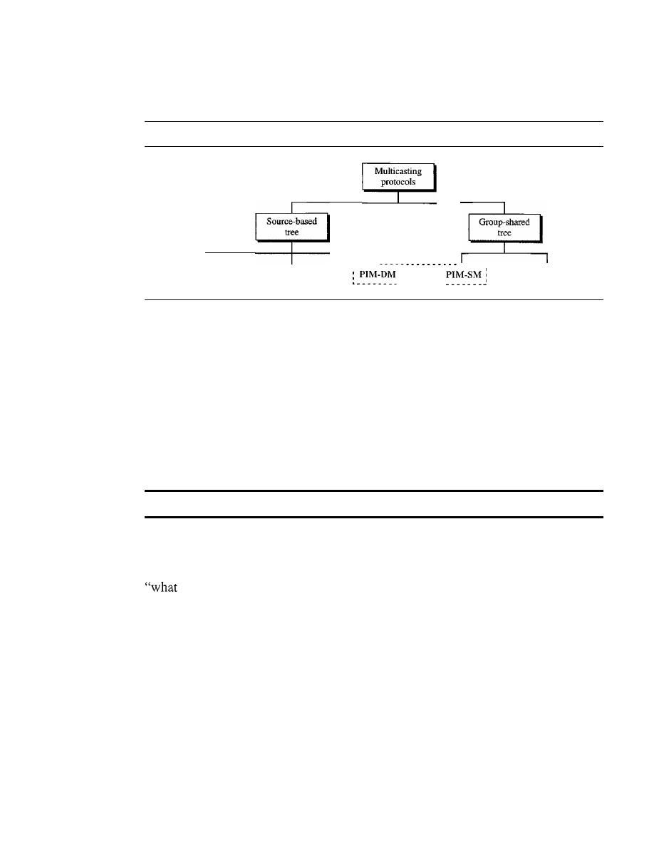
SECTION
22.4
MULTICAST ROUTING PROTOCOLS
685
We discuss these protocols in the remainder of this chapter. Figure 22.39 shows the
taxonomy of these protocols.
Figure 22.39
Taxonomy of common multicast protocols
----,
,
MOSPF
DVMRP
PIM
CRT
Multicast Link State Routing: MOSPF
In this section, we briefly discuss multicast link state routing and its implementation in
the Internet, MOSPF.
Multicast Link State Routing
We discussed unicast link state routing in Section 22.3.
We said that each router creates a shortest path tree by using Dijkstra's algorithm. The
routing table is a translation of the shortest path tree. Multicast
link
state routing is a
direct extension of unicast routing and uses a source-based tree approach. Although
unicast routing is quite involved, the extension to multicast routing is very simple and
straightforward.
Multicast
link
state routing uses the source-based tree approach.
Recall that in unicast routing, each node needs to advertise the state of its links. For
multicast routing, a node needs to revise the interpretation of
state. A node advertises
every group which has any loyal member on the link. Here the meaning of state is
groups are active on this link." The information about the group comes from
IGMP (see Chapter 21). Each router running IGMP solicits the hosts on the link to find
out the membership status.
When a router receives all these LSPs, it creates
n (n
is the number of groups)
topologies, from which
n
shortest path trees are made by using Dijkstra's algorithm. So
each router has a routing table that represents as many shortest path trees as there are
groups.
The only problem with this protocol is the time and space needed to create and
save the many shortest path trees. The solution is to create the trees only when needed.
When a router receives a packet with a multicast destination address, it runs the Dijkstra
algorithm to calculate the shortest path tree for that group. The result can be cached in
case there are additional packets for that destination.
MOSPF
Multicast Open Shortest Path First (MOSPF) protocol is an extension of
the OSPF protocol that uses multicast link state routing to create source-based trees.

686
CHAPTER
22
NETWORK LAYER: DELIVERY, FORWARDING, AND ROUTING
The protocol requires a new link state update packet to associate the unicast address of
a host with the group address or addresses the host is sponsoring. This packet is called
the group-membership LSA. In this way, we can include in the tree only the hosts
(using their unicast addresses) that belong to a particular group. In other words, we
make a tree that contains all the hosts belonging to a group, but we use the unicast
address of the host in the calculation. For efficiency, the router calculates the shortest
path trees on demand (when it receives the first multicast packet). In addition, the tree
can be saved in cache memory for future use by the same source/group pair. MOSPF is
a
data-driven
protocol; the first time an MOSPF router sees a datagram with a given
source and group address, the router constructs the Dijkstra shortest path tree.
Multicast Distance Vector: DVMRP
In this section, we briefly discuss multicast distance vector routing and its implementa-
tion in the Internet, DVMRP.
Multicast Distance Vector Routing
Unicast distance vector routing is very simple;
extending it to support multicast routing is complicated. Multicast routing does not
allow a router to send its routing table to its neighbors. The idea is to create a table from
scratch by using the information from the unicast distance vector tables.
Multicast distance vector routing uses source-based trees, but the router never
actually makes a routing table. When a router receives a multicast packet, it forwards
the packet as though it is consulting a routing table. We can say that the shortest path
tree is evanescent. After its use (after a packet is forwarded) the table is destroyed.
To accomplish this, the multicast distance vector algorithm uses a process based
on four decision-making strategies. Each strategy is built on its predecessor. We
explain them one by one and see how each strategy can improve the shortcomings of
the previous one.
D
Flooding.
Flooding is the first strategy that comes to mind. A router receives a
packet and, without even looking at the destination group address, sends it out
from every interlace except the one from which it was received. Flooding accom-
plishes the first goal of multicasting: every network with active members receives
the packet. However, so will networks without active members. This is a broadcast,
not a multicast. There is another problem: it creates loops. A packet that has left
the router may come back again from another interlace or the same interlace and
be forwarded again. Some flooding protocols keep a copy of the packet for a while
and discard any duplicates to avoid loops. The next strategy, reverse path forward-
ing, corrects this defect.
Flooding broadcasts packets, but creates loops in the systems.
o
Reverse Path Forwarding (RPF).
RPF is a modified flooding strategy. To prevent
loops, only one copy is forwarded; the other copies are dropped. In RPF, a router for-
wards only the copy that has traveled the shortest path from the source to the router.
To find this copy, RPF uses the unicast routing table. The router receives a packet and
extracts the source address (a unicast address).
It
consults its unicast routing table as
though it wants to send a packet to the source address. The routing table tells the
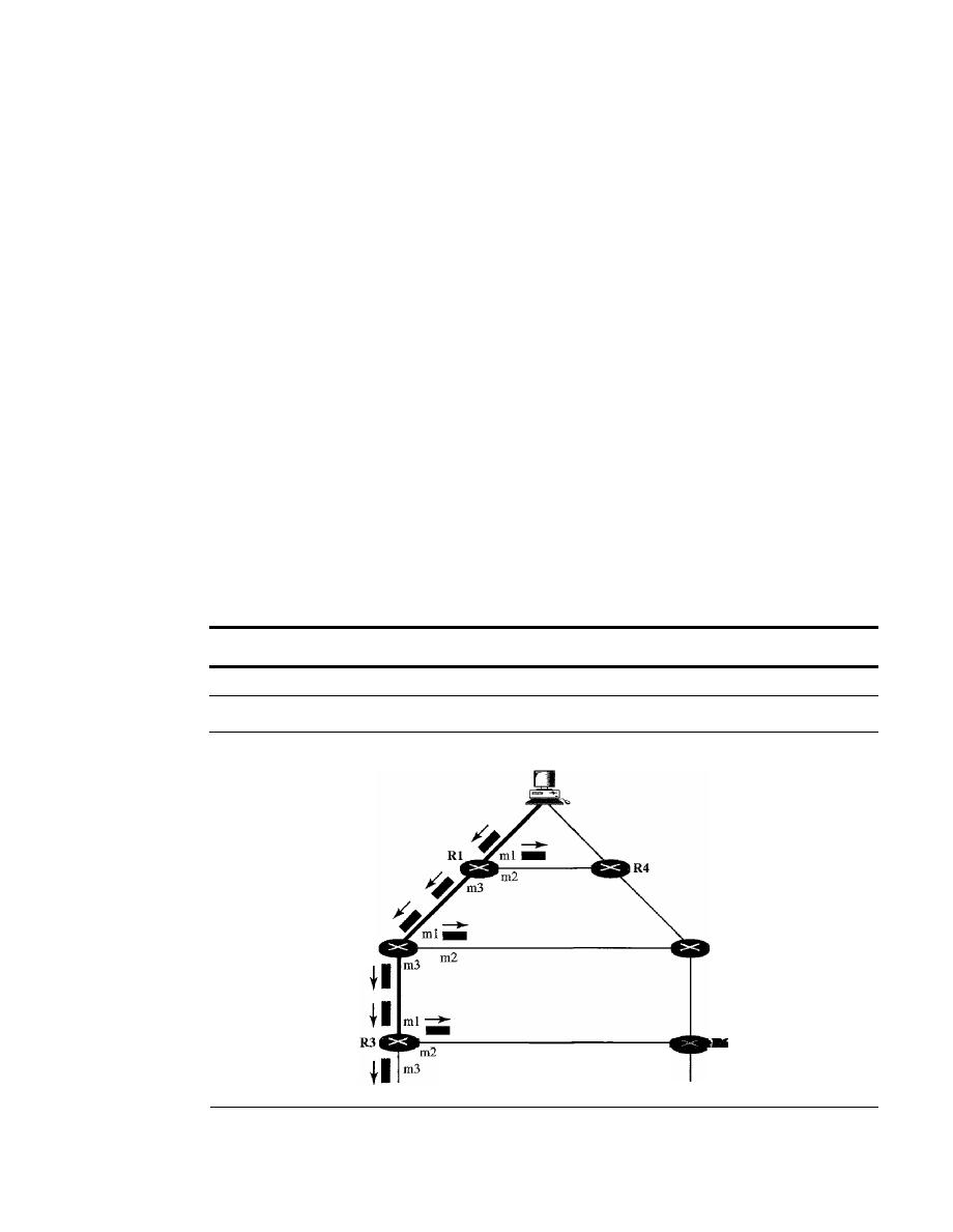
SECTION
22.4
MULTICAST ROUTING PROTOCOLS
687
router the next hop.
If
the multicast packet has just come from the hop defined in the
table, the packet has traveled the shortest path from the source to the router because
the shortest path is reciprocal in unicast distance vector routing protocols.
If
the path
from A to B is the shortest, then it is also the shortest from B to A. The router for-
wards the packet if it has traveled from the shortest path; it discards it otherwise.
This strategy prevents loops because there is always one shortest path from the
source to the router.
If
a packet leaves the router and comes back again, it has not trav-
eled the shortest path. To make the point clear, let us look at Figure 22.40.
Figure 22.40 shows part of a domain and a source. The shortest path tree as calcu-
lated by routers RI, R2, and R3 is shown by a thick line. When RI receives a packet
from the source through the interface rnl, it consults its routing table and finds that the
shortest path from RI to the source is through interface mI. The packet is forwarded.
However, if a copy of the packet has arrived through interface m2, it is discarded
because m2 does not define the shortest path from RI to the source. The story is the
same with R2 and R3. You may wonder what happens if a copy of a packet that arrives
at the ml interface of R3, travels through R6, R5, R2, and then enters R3 through inter-
face ml. This interface is the correct interface for R3. Is the copy of the packet for-
warded? The answer is that this scenario never happens because when the packet goes
from R5 to R2, it will be discarded by R2 and never reaches R3. The upstream routers
toward the source always discard a packet that has not gone through the shortest path,
thus preventing confusion for the downstream routers.
RPF eliminates the loop in the flooding process.
Figure 22.40
Reverse path forwarding (RPF)
Source
R2
R5
o
Reverse Path Broadcasting (RPB). RPF guarantees that each network receives a
copy of the multicast packet without formation of loops. However, RPF does not
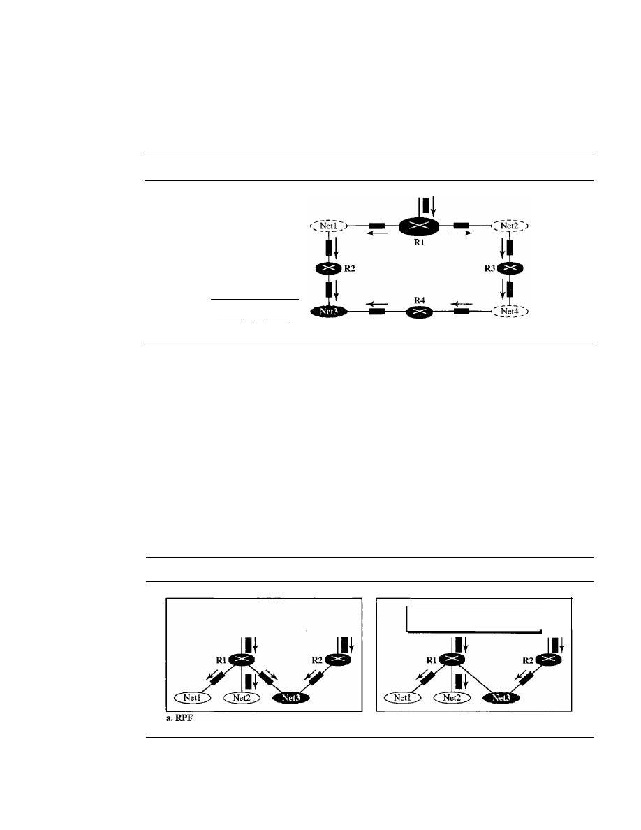
688
CHAPTER
22
NETWORK lAYER: DELWERY, FORWARDING, AND ROUTING
guarantee that each network receives only one copy; a network may receive two or
more copies. The reason is that RPF is not based on the destination address (a group
address); forwarding is based on the source address. To visualize the problem, let
us look at Figure 22.41.
Figure 22.41
Problem with
RPF
Net3 receives two
copies of the packet
b.RPB
Rl is the parent of Netl and Net2.
R2 is the parent of Net3
Net3 in this figure receives two copies of the packet even though each router
just sends out one copy from each interface. There is duplication because a tree has
not been made; instead of a tree we have a graph. Net3 has two parents: routers
R2
andR4.
To eliminate duplication, we must define only one parent router for each network.
We must have this restriction: A network can receive a multicast packet from a particular
source only through a designated parent router.
Now the policy is clear. For each source, the router sends the packet only out of those
interfaces for which it is the designated parent. This policy is called reverse path broad-
casting (RPB). RPB guarantees that the packet reaches every network and that every net-
work receives only one copy. Figure 22.42 shows the difference between RPF and RPB.
Figure 22.42
RPF
Versus
RPB
The reader may ask how the designated parent is determined. The designated parent
router can be the router with the shortest path to the source. Because routers periodically
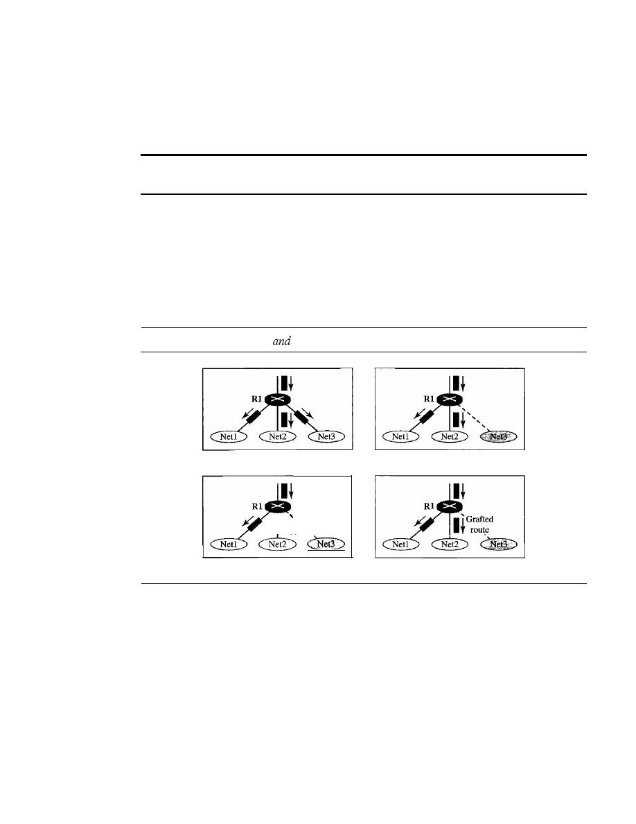
SECTION
22.4
MULTICAST ROUTING PROTOCOLS
689
send updating packets to each other (in RIP), they can easily determine which router in
the neighborhood has the shortest path to the source (when interpreting the source as the
destination), If more than one router qualifies, the router with the smallest IP address is
selected.
RPB creates a shortest path broadcast tree from the source to each destination.
It
guarantees that each destination receives one and only one copy of the packet.
o
Reverse Path Multicasting (RPM).
As you may have noticed, RPB does not
multicast the packet, it broadcasts it. This is not efficient. To increase efficiency,
the multicast packet must reach only those networks that have active members for
that particular group. This is called
reverse path multicasting
(RPM). To convert
broadcasting to multicasting, the protocol uses two procedures, pruning and graft-
ing. Figure 22.43 shows the idea of pruning and grafting.
Figure 22.43
RPF, RPB,
RPM
a.RPF
I
I
Pruned
I
route,
c. RPM (after pruning)
b.RPB
d. RPM (after grafting)
The designated parent router of each network is responsible for holding the mem-
bership information. This is done through the IGMP protocol described in Chapter 21.
The process starts when a router connected to a network finds that there is no interest in
a multicast packet. The router sends a
prune message
to the upstream router so that it
can exclude the corresponding interface. That is, the upstream router can stop sending
multicast messages for this group through that interface. Now if this router receives
prune messages from all downstream routers, it, in turn, sends a prune message to its
upstream router.
What if a leaf router (a router at the bottom of the tree) has sent a prune message
but suddenly realizes, through IGMP, that one of its networks is again interested in
receiving the multicast packet?
It
can send a
graft message.
The graft message forces
the upstream router to resume sending the multicast messages.
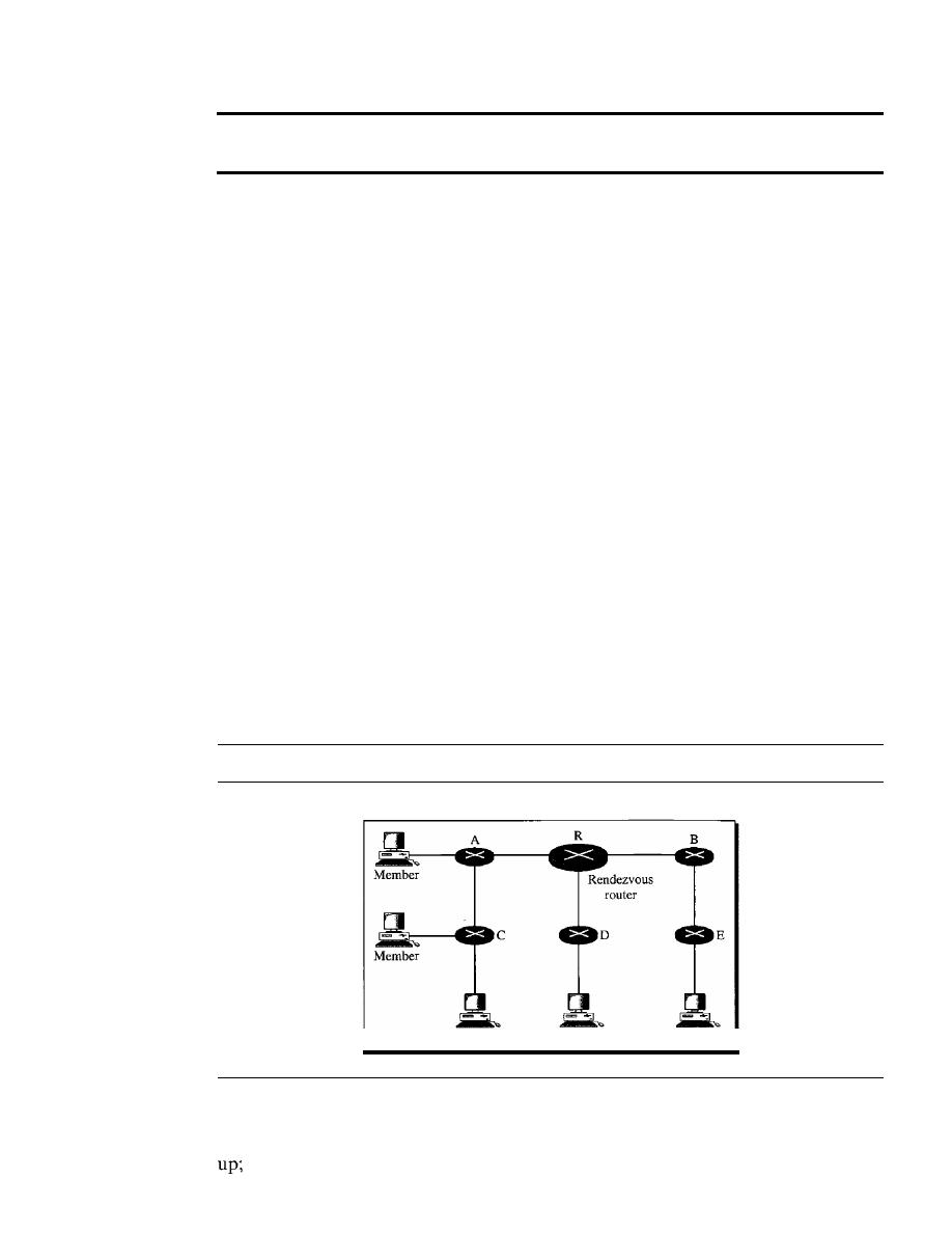
690
CHAPTER
22
NETWORK LAYER: DELIVERY, FORWARDING, AND ROUTING
RPM adds pruning and grafting to RPB to create a multicast shortest
path tree that supports dynamic membership changes.
DVMRP
The Distance Vector Multicast Routing Protocol (DVMRP) is an imple-
mentation of multicast distance vector routing.
It
is a source-based routing protocol,
based on RIP.
CRT
The Core-Based Tree (CBT) protocol is a group-shared protocol that uses a core as
the root of the tree. The autonomous system is divided into regions, and a core (center
router or rendezvous router) is chosen for each region.
Formation of the Tree
After the rendezvous point is selected, every router is infonned
of the unicast address of the selected router. Each router then sends a unicast join message
(similar to a grafting message) to show that it wants to join the group. This message passes
through all routers that are located between the sender and the rendezvous router. Each
intermediate router extracts the necessary infonnation from the message, such as the
unicast address of the sender and the interface through which the packet has arrived, and
forwards the message to the next router in the path. When the rendezvous router has
received all join messages from every member of the group, the tree is formed. Now
every router knows its upstream router (the router that leads to the root) and the down-
stream router (the router that leads to the leaf).
If
a router wants to leave the group, it sends a leave message to its upstream router.
The upstream router removes the link to that router from the tree and forwards the mes-
sage to its upstream router, and so on. Figure 22.44 shows a group-shared tree with its
rendezvous router.
Figure 22.44
Group-shared tree with rendezvous router
Shared tree
Member
Member
Member
The reader may have noticed two differences between DVMRP and MOSPF, on
one hand, and CBT, on the other. First, the tree for the first two is made from the root
the tree for CBT is fonned from the leaves down. Second, in DVMRP, the tree is
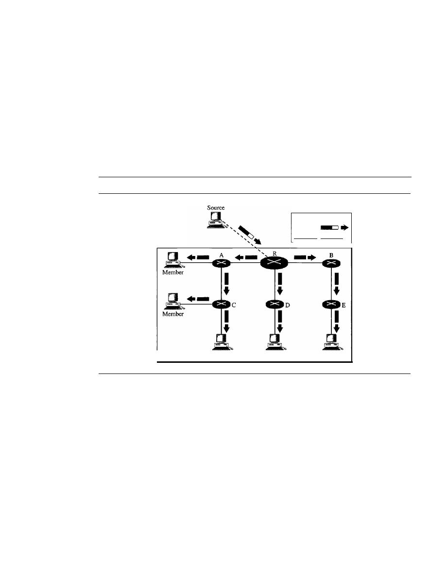
SECTION
22.4
MULTICAST ROUTING PROTOCOLS
691
first made (broadcasting) and then pruned; in CBT, there is no tree at the beginning; the
joining (grafting) gradually makes the tree.
Sending Multicast Packets
After formation of the tree, any source (belonging to the
group or not) can send a multicast packet to all members of the group.
It
simply sends
the packet to the rendezvous router, using the unicast address of the rendezvous router;
the rendezvous router distributes the packet to all members of the group. Figure 22.45
shows how a host can send a multicast packet to all members of the group. Note that the
source host can be any of the hosts inside the shared tree or any host outside the shared
tree. In Figure 22.45 we show one located outside the shared tree.
Figure 22.45
Sending a multicast packet to the rendezvous router
Shared tree
Member
Member
Legend
Unicast
MulLicast _ .
Member
Selecting the Rendezvous Router
This approach is simple except for one point.
How do we select a rendezvous router to optimize the process and multicasting as well?
Several methods have been implemented. However, this topic is beyond the scope of
this book, and we leave it to more advanced books.
In summary, the Core-Based Tree (CBT) is a group-shared tree, center-based pro-
tocol using one tree per group. One of the routers in the tree is called the core. A packet
is sent from the source to members of the group following this procedure:
1. The source, which mayor may not be part of the tree, encapsulates the multicast
packet inside a unicast packet with the unicast destination address of the core and
sends it to the core. This part of delivery is done using a unicast address; the only
recipient is the core router.
2. The core decapsulates the unicast packet and forwards it to all interested intetfaces.
3. Each router that receives the multicast packet, in tum, forwards it to all interested
interfaces.

692
CHAPTER 22
NETWORK LAYER: DELIVERY, FORWARDING, AND ROUTING
In
CRT, the source sends the multicast packet (encapsulated in a unicast packet) to the core
router. The core router decapsulates the packet and forwards it
to
all
interested interfaces.
PIM
Protocol Independent Multicast (PIM)
is the name given to two independent multicast
routing protocols:
Protocol Independent Multicast, Dense Mode (PIM-DM)
and
Protocol Independent Multicast, Sparse Mode (PIM-SM).
Both protocols are unicast-
protocol-dependent, but the similarity ends here. We discuss each separately.
PIM-DM
PIM-DM is used when there is a possibility that each router is involved in
multicasting
(dense mode).
In this environment, the use of a protocol that broadcasts
the packet is justified because almost all routers are involved in the process.
PIM-DM is used in a dense multicast environment, such as a LAN.
PIM-DM is a source-based tree routing protocol that uses RPF and pruning and
grafting strategies for multicasting. Its operation is like that of DVMRP; however,
unlike DVMRP, it does not depend on a specific unicasting protocol. It assumes that the
autonomous system is using a unicast protocol and each router has a table that can find
the outgoing interface that has an optimal path to a destination. This unicast protocol
can be a distance vector protocol (RIP) or link state protocol (OSPF).
PIM-DM uses RPF and pruning and grafting strategies to handle multicasting.
However, it is independent of the underlying unicast protocol.
PIM-SM
PIM-SM is used when there is a slight possibility that each router is involved
in multicasting (sparse mode). In this environment, the use of a protocol that broadcasts
the packet is not justified; a protocol such as CBT that uses a group-shared tree is more
appropriate.
PIM-SM is used in a sparse multicast environment such as a WAN.
PIM-SM is a group-shared tree routing protocol that has a rendezvous point (RP)
as the source of the tree. Its operation is like CBT; however, it is simpler because it does
not require acknowledgment from ajoin message. In addition, it creates a backup set of
RPs for each region to cover RP failures.
One of the characteristics of PIM-SM is that it can switch from a group-shared tree
strategy to a source-based tree strategy when necessary. This can happen if there is a
dense area of activity far from the RP. That area can be more efficiently handled with a
source-based tree strategy instead of a group-shared tree strategy.
PIM-SM is similar to CRT but uses a simpler procedure.
MBONE
Multimedia and real-time communication have increased the need for multicasting in
the Internet. However, only a small fraction of Internet routers are multicast routers. In
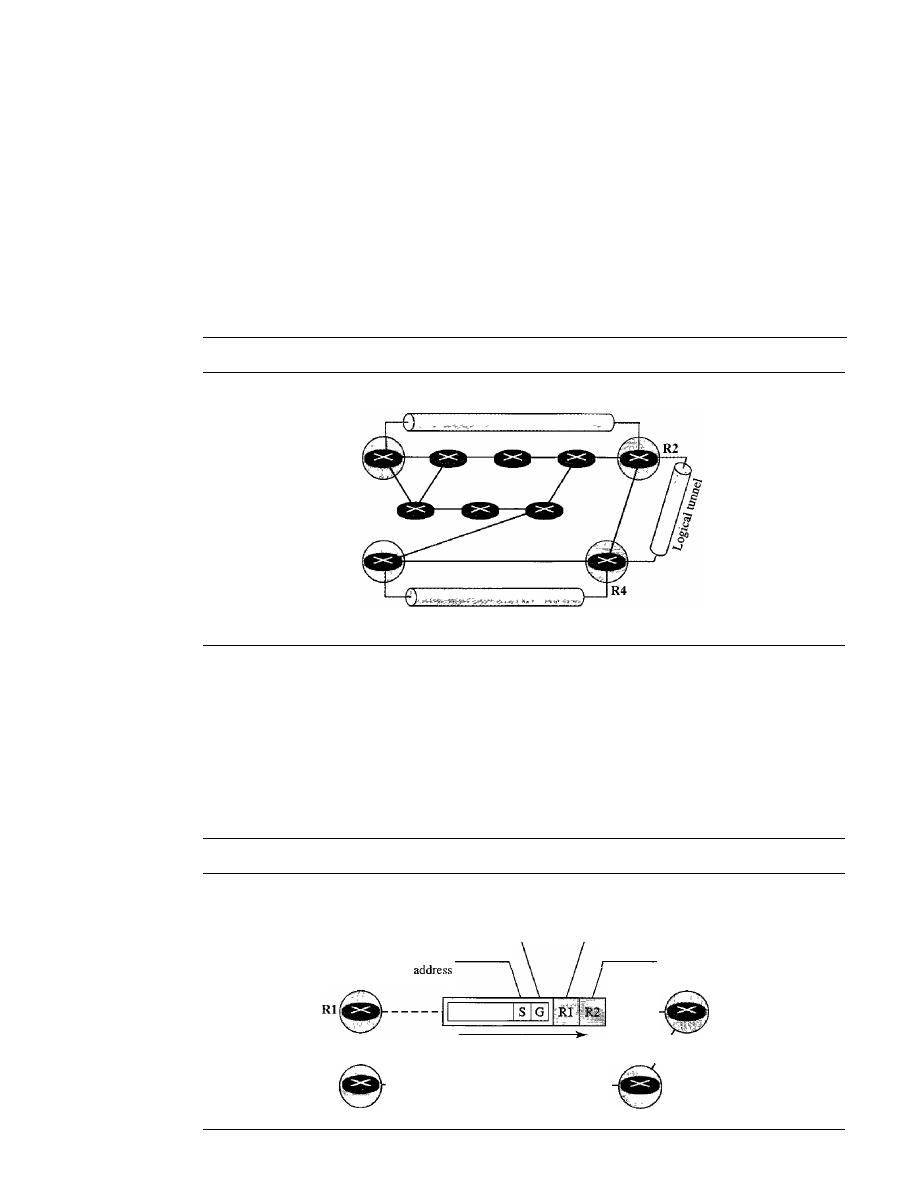
SECTION
22.4
MULTICAST ROUTING PROTOCOLS
693
other words, a multicast router may not find another multicast router in the neighbor-
hood to forward the multicast packet. Although this problem may be solved in the next
few years by adding more and more multicast routers, there is another solution to this
problem. The solution is tunneling. The multicast routers are seen as a group of routers
on top of unicast routers. The multicast routers may not be connected directly, but they
are connected logically. Figure 22.46 shows the idea. In Figure 22.46, only the routers
enclosed in the shaded circles are capable of multicasting. Without tunneling, these routers
are isolated islands. To enable multicasting, we make a multicast backbone (MBONE)
out of these isolated routers by using the concept of tunneling.
Figure 22.46
Logical tunneling
Logical tunnel
Rl
R3
Logical tunnel
A logical tunnel is established by encapsulating the multicast packet inside a uni-
cast packet. The multicast packet becomes the payload (data) of the unicast packet. The
intermediate (nonmulticast) routers forward the packet as unicast routers and deliver
the packet from one island to another. It's as if the unicast routers do not exist and the
two multicast routers are neighbors. Figure 22.47 shows the concept. So far the only
protocol that supports MBONE and tunneling is DVMRP.
Figure 22.47
MBONE
- - - - -
R2
Unicast
destination
address
(router R2)
Unicast source
address
(router RI)
Multicast
group
address
Source
I
I
I
R3
----------------------
R4

694
CHAPTER
22
NETWORK LAYER: DELIVERY, FORWARDING, AND ROUTING
22.5
RECOMMENDED READING
For more details about subjects discussed in this chapter, we recommend the following
books and sites. The items in brackets [...
J
refer to the reference list at the end of the text.
Books
Delivery and forwarding are discussed in Chapter 6 of [For06]. Unicast routing protocols
are discussed in Chapter 14 of [For06]. Multicasting and multicast routing are discussed
in Chapter 15 of [For06]. For a complete discussion of multicasting see [WZOl]. For
routing protocols see [HuiOO]. OSPF is discussed in [Moy98].
Sites
o
www.ietf.org/rfc.html Information about RFCs
RFCs
A discussion of RIP can be found in the following RFCs:
1131,1245,1246,1247,1370,1583,1584,1585, 1586,1587, 1722,1723,2082,2453
A discussion of OSPF can be found in the following RFCs:
1131,1245,1246,1247,1370,1583,1584,1585, 1586, 1587,2178,2328,2329,2370
A discussion of BGP can be found in the following RFCs:
1092,1105,1163,1265,1266,1267,1364,1392,1403, 1565,1654,1655,1665,1771,1772,
1745,1774,2283
22.6
KEY TERMS
address aggregation
area
area border routers
area identification
autonomous system (AS)
backbone router
Border Gateway Protocol (BGP)
broadcasting
Core-Based Tree (CBT) protocol
data-driven
default method
delivery
designated parent router
Dijkstra's algorithm
direct delivery
distance learning
Distance Vector Multicast Routing
Protocol (DVMRP)
distance vector routing
distributed database
dynamic routing method
dynamic routing table
flooding
forwarding
graft message
group-shared tree

hierarchical routing
hop count
host-specific method
ifconfig
immediate neighbors
indirect delivery
interdomain routing
intradomain routing
least-cost tree
link state routing
logical tunnel
longest mask matching
metric
multicast backbone (MBONE)
Multicast Open Shortest Path First
(MOSPF)
multicast router
multicast routing
multicasting
multiple unicasting
netstat
network-specific method
next-hop address
next-hop method
Open Shortest Path First (OSPF)
optional attribute
OSPF protocol
path vector routing
point-to-point link
poison reverse
policy routing
SECTION
22.7
SUMMARY
695
Protocol Independent Multicast (PIM)
Protocol Independent Multicast, Dense
Mode (PIM-DM)
Protocol Independent Multicast, Sparse
Mode (PIM-SM)
prune message
rendezvous router
rendezvous-point tree
reverse path broadcasting (RPB)
reverse path forwarding (RPF)
reverse path multicasting (RPM)
route method
routing
Routing Information Protocol (RIP)
routing protocols
shortest path tree
slow convergence
source-based tree
speaker node
split horizon
static routing table
stub link
switching fabric
teleconferencing
transient link
triggered update
tunneling
unicasting
update message
virtual link
attribute
22.7
SUMMARY
o
The delivery of a packet is called direct if the deliverer (host or router) and the des-
tination are on the same network; the delivery of a packet is called indirect if the
deliverer (host or router) and the destination are on different networks.
o
In the next-hop method, instead of a complete list of the stops the packet must
make, only the address of the next hop is listed in the routing table; in the network-
specific method, all hosts on a network share one entry in the routing table.

696
CHAPTER
22
NETWORK LAYER: DELIVERY, FORWARDING, AND ROUTING
D
In the host-specific method, the full IP address of a host is given in the routing table.
D
In the default method, a router is assigned to receive all packets with no match in
the routing table.
D
The routing table for classless addressing needs at least four columns.
D
Address aggregation simplifies the forwarding process in classless addressing.
o
Longest mask matching is required in classless addressing.
o
Classless addressing requires hierarchical and geographical routing to prevent
immense routing tables.
D
A static routing table's entries are updated manually by an administrator; a dynamic
routing table's entries are updated automatically by a routing protocol.
D
A metric is the cost assigned for passage of a packet through a network.
D
An autonomous system (AS) is a group of networks and routers under the authority
of a single administration.
D
RIP is based on distance vector routing, in which each router shares, at regular
intervals, its knowledge about the entire AS with its neighbors.
D
Two shortcomings associated with the RIP protocol are slow convergence and
instability. Procedures to remedy RIP instability include triggered update, split
horizons, and poison reverse.
D
OSPF divides an AS into areas, defined as collections of networks, hosts, and
routers.
o
OSPF is based on link state routing, in which each router sends the state of its
neighborhood to every other router in the area. A packet is sent only if there is a
change in the neighborhood.
D
OSPF routing tables are calculated by using Dijkstra's algorithm.
D
BGP is an interautonomous system routing protocol used to update routing tables.
D
BGP is based on a routing protocol called path vector routing. In this protocol, the
ASs through which a packet must pass are explicitly listed.
o
In a source-based tree approach to multicast routing, the source/group combination
determines the tree; in a group-shared tree approach to multicast routing, the
determines the tree.
D
MOSPF is a multicast routing protocol that uses multicast link state routing to
create a source-based least-cost tree.
D
In reverse path forwarding (RPF) , the router forwards only the packets that have
traveled the shortest path from the source to the router.
D
Reverse path broadcasting (RPB) creates a shortest path broadcast tree from the
source to each destination.
It
guarantees that each destination receives one and
only one copy of the packet.
D
Reverse path multicasting (RPM) adds pruning and grafting to RPB to create a
multicast shortest path tree that supports dynamic membership changes.
D
DVMRP is a multicast routing protocol that uses the distance routing protocol to
create a source-based tree.
D
The Core-Based Tree (CBT) protocol is a multicast routing protocol that uses a
router as the root of the tree.

SECTION
22.8
PRACTICE SET
697
D
PIM-DM is a source-based tree routing protocol that uses RPF and pruning and
grafting strategies to handle multicasting.
o
PIM-SM is a group-shared tree routing protocol that is similar to CBT and uses a
rendezvous router as the source of the tree.
D
For multicasting between two noncontiguous multicast routers, we make a multicast
backbone (MBONE) to enable tunneling.
22.8
PRACTICE
SET
Review Questions
1. What is the difference between a direct and an indirect delivery?
2. List three forwarding techniques discussed in this chapter and give a brief description
of each.
3. Contrast two different routing tables discussed in this chapter.
4. What is the purpose of RIP?
5. What are the functions of a RIP message?
6. Why is the expiration timer value 6 times that of the periodic timer value?
7. How does the hop count limit alleviate RIP's problems?
8. List RIP shortcomings and their corresponding fixes.
9. What is the basis of classification for the four types of links defined by OSPF?
10. Why do OSPF messages propagate faster than RIP messages?
11. What is the purpose of BGP?
12. Give a brief description of two groups of multicast routing protocols discussed in
this chapter.
Exercises
13. Show a routing table for a host that is totally isolated.
14. Show a routing table for a host that is connected to a LAN without being connected
to the Internet.
15. Find the topology of the network if Table 22.3 is the routing table for router R 1.
Table 22.3
Routing table for Exercise 15
Network
Next-Hop
Mask
Address
Address
Interface
/27
202.14.17.224
-
rn1
/18
145.23.192.0
-
rnO
Default
Default
130.56.12.4
m2
16. Can router R1 in Figure 22.8 receive a packet with destination address 140.24.7.194?
Explain your answer.

698
CHAPTER 22
NETWORK LAYER: DEUVERY, FORWARDING, AND ROUTING
17. Can router Rl in Figure 22.8 receive a packet with destination address l40.24.7.42?
Explain your answer.
18. Show the routing table for the regional ISP in Figure 22.9.
19. Show the routing table for local ISP 1 in Figure 22.9.
20. Show the routing table for local ISP 2 in Figure 22.9.
21. Show the routing table for local ISP 3 in Figure 22.9.
22. Show the routing table for small ISP 1 in Figure 22.9.
23. Contrast and compare distance vector routing with link state routing.
24. A router has the following RIP routing table:
Net!
Net2
Net3
Net4
4
2
!
5
B
C
F
G
What would be the contents of the table if the router received the following RIP
message from router C?
Net!
2
Net2
!
Net3
3
Net4
7
25. How many bytes are empty in a RIP message that advertises
N
networks?
26. A router has the following RIP routing table:
Net!
Net2
Net3
Net4
4
2
1
5
B
C
F
G
Show the response message sent by this router.
27. Show the autonomous system with the following specifications:
a. There are eight networks (Nl to N8).
b. There are eight routers (Rl to R8).
c. Nl, N2, N3, N4, NS, and N6 are Ethernet LANs.
d. N7 and N8 are point-to-point WANs.
e. Rl connects Nl and N2.
f.
R2 connects Nl and N7.
g. R3 connects N2 and N8.
h. R4 connects N7 and N6.
i. RS connects N6 and N3.
j. R6 connects N6 and N4.
k. R7 connects N6 and NS.
1. R8 connects N8 and N5.

SECTION
22.8
PRACTICE SET
699
28. Draw the graphical representation of the autonomous system of Exercise 27 as
seen by OSPF.
29. Which of the networks in Exercise 27 is a transient network? Which is a stub
network?
30. A router using DVMRP receives a packet with source address 10.14.17.2 from
interface 2. If the router forwards the packet, what are the contents of the entry
related to this address in the unicast routing table?
31. Does RPF actually create a shortest path tree? Explain.
32. Does RPB actually create a shortest path tree? Explain. What are the leaves of
the tree?
33. Does RPM actually create a shortest path tree? Explain. What are the leaves of
the tree?
Research Activities
34.
If
you have access to UNIX (or LINUX), use
netstat
and
ifconfig
to find the routing
table for the server to which you are connected.
35. Find out how your ISP uses address aggregation and longest mask match principles.
36. Find out whether your IP address is part of the geographical address allocation.
37. If you are using a router, find the number and names of the columns in the routing
table.


Transport Layer
Objectives
The transport layer is responsible for process-to-process delivery of the entire message.
A process is an application program running on a host. Whereas the network layer
oversees source-to-destination delivery of individual packets, it does not recognize any
relationship between those packets.
It
treats each one independently, as though each
piece belonged to a separate message, whether or not it does. The transport layer, on the
other hand, ensures that the whole message arrives intact and in order, overseeing both
error control and flow control at the source-to-destination level.
The transport layer is responsible for the delivery
of a message from one process to another.
Computers often run several programs at the same time. For this reason, source-
to-destination delivery means delivery not only from one computer to the next but also
from a specific process on one computer to a specific process on the other. The transport
layer header must therefore include a type of address called a
service-point address
in
the OSI model and port number or port addresses in the Internet and TCP/IP protocol
suite.
A transport layer protocol can be either connectionless or connection-oriented.
A connectionless transport layer treats each segment as an independent packet and
delivers it to the transport layer at the destination machine. A connection-oriented
transport layer makes a connection with the transport layer at the destination machine
first before delivering the packets. After all the data is transferred, the connection is
terminated.
In the transport layer, a message is normally divided into transmittable segments. A
connectionless protocol, such as UDP, treats each segment separately. A connection-
oriented protocol, such as TCP and SCTP, creates a relationship between the segments
using sequence numbers.
Like the data link layer, the transport layer may be responsible for flow and error
control. However, flow and error control at this layer is performed end to end rather
than across a single link. We will see that one of the protocols discussed in this part of

the book, UDP, is not involved in flow or error controL On the other hand, the other two
protocols, TCP and SCTP, use sliding windows for flow control and an acknowledgment
system for error controL
Part 5 of the book is devoted to the transport layer
and the services provided by this layer.
Chapters
This part consists of two chapters: Chapters 23 and 24.
Chapter 23
Chapter 23 discusses three transport layer protocols in the Internet: UDP, TCP, and
SCTP. The first, User Datagram Protocol (UDP), is a connectionless, unreliable proto-
col that is used for its efficiency. The second, Transmission Control Protocol (TCP), is a
connection-oriented, reliable protocol that is a good choice for data transfer. The third,
Stream Control Transport Protocol (SCTP) is a new transport-layer protocol designed
for multimedia applications.
Chapter 24
Chapter 24 discuss two related topics: congestion control and quality of service. Although
these two issues can be related to any layer, we discuss them here with some references to
other layers.

CHAPTER 23
Process-la-Process Delivery:
UDp, TCp, and SCTP
We begin this chapter by giving the rationale for the existence of the
transport layer-
the need for process-to-process delivery. We discuss the issues arising from this type of
delivery, and we discuss methods to handle them.
The Internet model has three protocols at the transport layer: UDP, TCP, and SCTP.
First we discuss UDP, which is the simplest of the three. We see how we can use this
very simple transport layer protocol that lacks some of the features of the other two.
We then discuss TCP, a complex transport layer protocol. We see how our previously
presented concepts are applied to TCP. We postpone the discussion of congestion control
and quality of service in TCP until Chapter 24 because these two topics apply to the data
link layer and network layer as well.
We finally discuss SCTP, the new transport layer protocol that is designed for
multihomed, multistream applications such as multimedia.
23.1
PROCESS-TO-PROCESS DELIVERY
The data link layer is responsible for delivery of frames between two neighboring nodes
over a link. This is called node-to-node delivery. The network layer is responsible for
delivery of datagrams between two hosts. This is called host-to-host delivery. Communi-
cation on the Internet is not defined as the exchange of data between two nodes or
between two hosts. Real communication takes place between two processes (application
programs). We need
process-to-process delivery.
However, at any moment, several pro-
cesses may be running on the source host and several on the destination host. To complete
the delivery, we need a mechanism to deliver data from one of these processes running on
the source host to the corresponding process running on the destination host.
The transport layer is responsible for process-to-process delivery-the delivery of
a packet, part of a message, from one process to another. Two processes communicate
in a client/server relationship, as we will see later. Figure 23.1 shows these three types
of deliveries and their domains.
The transport layer is responsible for process-to-process delivery.
703
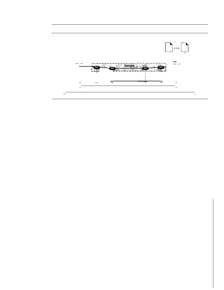
704
CHAPTER
23
PROCESS-TO-PROCESS DELIVERY: UDp, TCp, AND SCTP
Figure 23.1
Types of data deliveries
Processes
D···D
Node to node: Data link layer
Host to host: Network layer
Process to process: Transport layer
Processes
\
\
\
\
\
\
\
\
\
\
\
\
\
\
"
I
'I
-
I
I
Node to : Node to
:
node
1
node
I
,I
Host to host
Node to node
Process to process
I
I
I
I
I
I
I
Node to
I Node to I
I
node
I
node
I
II
'II
I
I'
=
-
1
1
I
I
I
I
I
I
I
1
I
/
/
/'
Client/Server Paradigm
Although there are several ways to achieve process-to-process communication, the most
common one is through the client/server paradigm. A process on the local host, called
a client, needs services from a process usually on the remote host, called a server.
Both processes (client and server) have the same name. For example, to get the day
and time from a remote machine, we need a Daytime client process running on the
local host and a Daytime server process running on a remote machine.
Operating systems today support both multiuser and multiprogramming environ-
ments. A remote computer can run several server programs at the same time, just as
local computers can run one or more client programs at the same time. For communica-
tion, we must define the following:
1. Local host
2. Local process
3. Remote host
4. Remote process
Addressing
Whenever we need to deliver something to one specific destination among many, we need
an address. At the data link layer, we need a MAC address to choose one node among sev-
eral nodes if the connection is not point-to-point. A frame in the data link layer needs a
destination MAC address for delivery and a source address for the next node's reply.
At the network layer, we need an IP address to choose one host among millions. A
datagram in the network layer needs a destination IP address for delivery and a source
IP address for the destination's reply.
At the transport layer, we need a transport layer address, called a port number, to
choose among multiple processes running on the destination host. The destination port
number is needed for delivery; the source port number is needed for the reply.
In the Internet model, the port numbers are 16-bit integers between 0 and 65,535.
The client program defines itself with a port number, chosen randomly by the transport
layer software running on the client host. This is the ephemeral port number.
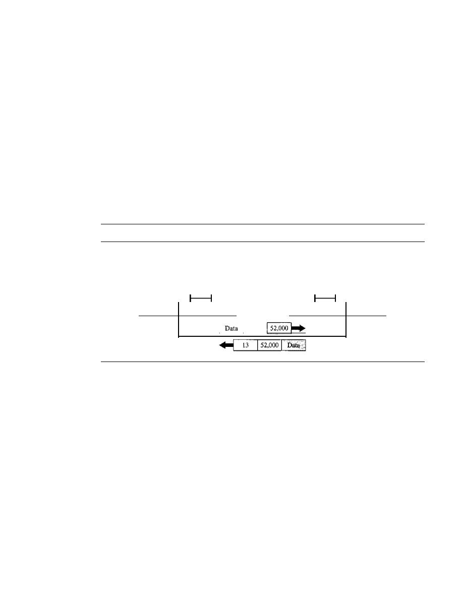
SECTION
23.1
PROCESS-TV-PROCESS DELWERY
705
The server process must also define itself with a port number. This port number,
however, cannot be chosen randomly.
If
the computer at the server site runs a server
process and assigns a random number as the port number, the process at the client site
that wants to access that server and use its services will not know the port number. Of
course, one solution would be to send a special packet and request the port number of a
specific server, but this requires more overhead. The Internet has decided to use universal
port numbers for servers; these are called
well-known port numbers.
There are some
exceptions to this rule; for example, there are clients that are assigned well-known port
numbers. Every client process knows the well-known port number of the corresponding
server process. For example, while the Daytime client process, discussed above, can
use an ephemeral (temporary) port number 52,000 to identify itself, the Daytime server
process must use the well-known (permanent) port number 13. Figure 23.2 shows this
concept.
Figure 23.2
Port numbers
Daytime
client
DD D
H
52,000
Transport layer
Daytime
server
D DD
13
H
Transport layer
I
I
13
It should be clear by now that the IP addresses and port numbers play different
roles in selecting the final destination of data. The destination IP address defines the
host among the different hosts in the world. After the host has been selected, the port
number defines one of the processes on this particular host (see Figure 23.3).
lANA Ranges
The lANA (Internet Assigned Number Authority) has divided the port numbers into
three ranges: well known, registered, and dynamic (or private), as shown in Figure 23.4.
o
Well-known ports.
The ports ranging from 0 to 1023 are assigned and controlled
by lANA. These are the well-known ports.
o
Registered ports.
The ports ranging from 1024 to 49,151 are not assigned or con-
trolled by lANA. They can only be registered with lANA to prevent duplication.
o
Dynamic ports.
The ports ranging from 49,152 to 65,535 are neither controlled
nor registered. They can be used by any process. These are the ephemeral ports.
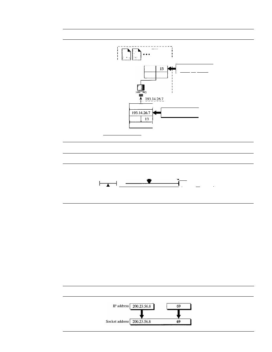
706
CHAPTER
23
PROCESS-TO-PROCESS DELIVERY: UDp, TCP, AND SCTP
Figure 23.3
IP addresses versus port numbers
I
I
I
I
I
I
I
I
I
I
I
I
I
I
I
J
I
:
:
Port number
selects the process
IP header
Transport layer
header
Figure 23.4
lANA ranges
IP address
selects the host
Dynamic
Registered
o
1023
I
49,152
1--1
I
f
T
1024
49,151
Well known
65,535
I
Socket Addresses
Process-to-process delivery needs two identifiers, IP address and the port number, at
each end to make a connection. The combination of an IP address and a port number is
called a socket address. The client socket address defines the client process uniquely
just as the server socket address defines the server process uniquely (see Figure 23.5).
A transport layer protocol needs a pair of socket addresses: the client socket address
and the server socket address. These four pieces of information are part of the IP header
and the transport layer protocol header. The IP header contains the IP addresses; the
UDP or TCP header contains the port numbers.
Figure 23.5
Socket address
Port number
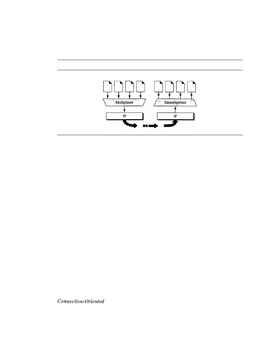
SECTION
23.1
PROCESS-TO-PROCESS DELIVERY
707
Multiplexing and Demultiplexing
The addressing mechanism allows multiplexing and demultiplexing by the transport
layer, as shown in Figure 23.6.
Figure 23.6
Multiplexing and demultiplexing
Processes
Processes
Multiplexing
At the sender site, there may be several processes that need to send packets. However,
there is only one transport layer protocol at any time. This is a many-to-one relationship
and requires multiplexing. The protocol accepts messages from different processes,
differentiated by their assigned port numbers. After adding the header, the transport layer
passes the packet to the network layer.
Demultiplexing
At the receiver site, the relationship is one-to-many and requires demultiplexing. The
transport layer receives datagrams from the network layer. After error checking and
dropping of the header, the transport layer delivers each message to the appropriate
process based on the port number.
Connectionless Versus Connection-Oriented Service
A transport layer protocol can either be connectionless or connection-oriented.
Connectionless Service
In a connectionless service, the packets are sent from one party to another with no need
for connection establishment or connection release. The packets are not numbered; they
may be delayed or lost or may arrive out of sequence. There is no acknowledgment
either. We
will
see shortly that one of the transport layer protocols in the Internet model,
UDP, is connectionless.
Service
In a connection-oriented service, a connection is first established between the sender
and the receiver. Data are transferred. At the end, the connection is released. We will see
shortly that TCP and SCTP are connection-oriented protocols.
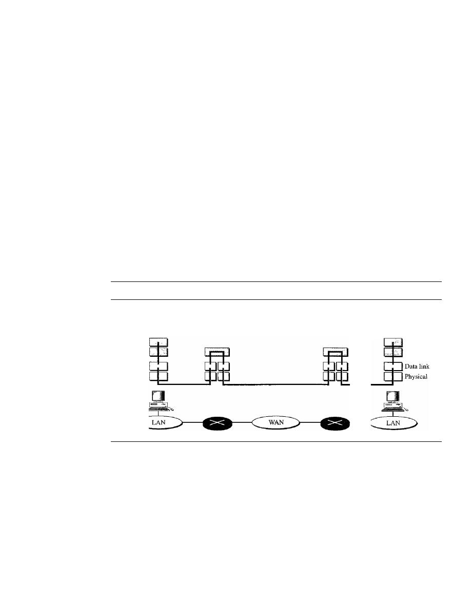
708
CHAPTER
23
PRO CESS- TO-PROCESS DELNERY: UDp, TCp, AND SCTP
Reliable Versus Unreliable
The transport layer service can be reliable or unreliable. If the application layer program
needs reliability, we use a reliable transport layer protocol by implementing flow and
error control at the transport layer. This means a slower and more complex service. On
the other hand, if the application program does not need reliability because it uses its
own flow and error control mechanism or it needs fast service or the nature of the service
does not demand flow and error control (real-time applications), then an unreliable
protocol can be used.
In the Internet, there are three common different transport layer protocols, as we have
already mentioned. UDP is connectionless and unreliable; TCP and SCTP are connection-
oriented and reliable. These three can respond to the demands of the application layer
programs.
One question often comes to the mind.
If
the data link layer is reliable and has flow
and error control, do we need this at the transport layer, too? The answer is yes. Reliability
at the data link layer is between two nodes; we need reliability between two ends. Because
the network layer in the Internet is unreliable (best-effort delivery), we need to implement
reliability at the transport layer. To understand that error control at the data link layer does
not guarantee error control at the transport layer, let us look at Figure 23.7.
Figure 23.7
Error control
-
Error is checked in these paths by the data link layer
-
Error is not checked in these paths by the data link layer
Transport
Network
Transport
Network
Data link
Physical
As we will see, flow and error control in TCP is implemented by the sliding window
protocol, as discussed in Chapter 11. The window, however, is character-oriented,
instead of frame-oriented.
Three Protocols
The original TCP/IP protocol suite specifies two protocols for the transport layer: UDP
and TCP. We first focus on UDP, the simpler of the two, before discussing TCP. A new
transport layer protocol, SCTP, has been designed, which we also discuss in this chapter.
Figure 23.8 shows the position of these protocols in the TCP/IP protocol suite.
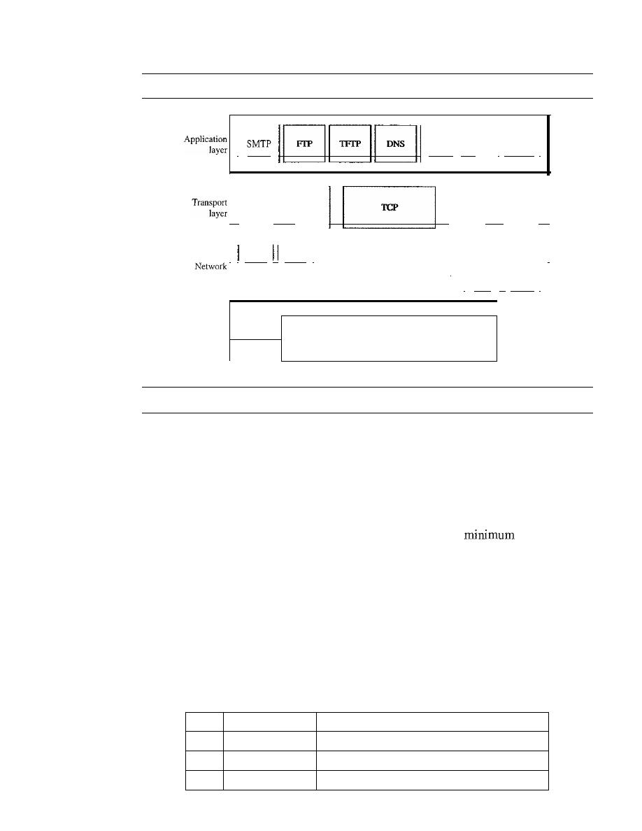
SECTION
23.2
USER DATAGRAM PROTOCOL (UDP)
709
Figure 23.8
Position of UDp, TCp, and SCTP in TCPIIP suite
I
SNMP
1·.. 1
BOOTP
I
Underlying LAN or WAN
technology
Physical
layer
II
SCTP
II
UDP
II
I
IGMP
ICMP
I
I
IT
I
layer
I
ARP
II
RARP
I
Data link
layer
23.2
USER DATAGRAM PROTOCOL (UDP)
The
User Datagram Protocol (UDP)
is called a
connectionless, unreliable transport
protocol.
It
does not add anything to the services of IP except to provide process-to-
process communication instead of host-to-host communication. Also, it performs very
limited error checking.
If
UDP is so powerless, why would a process want to use it? With the disadvantages
come some advantages. UDP is a very simple protocol using a
of overhead. If
a process wants to send a small message and does not care much about reliability, it can
use UDP. Sending a small message by using UDP takes much less interaction between
the sender and receiver than using TCP or SCTP.
Well-Known Ports for UDP
Table 23.1 shows some well-known port numbers used by UDP. Some port numbers
can be used by both UDP and TCP. We discuss them when we talk about TCP later in
the chapter.
Table 23.1
Well-known ports used with UDP
Port
Protocol
Description
7
Echo
Echoes a received datagram back to the sender
9
Discard
Discards any datagram that is received
11
Users
Active users

710
CHAPTER
23
PROCESS-TO-PROCESS DELIVERY: UDp, TCp, AND SCTP
Table 23.1
Well-known ports used with UDP (continued)
Port
Protocol
Description
13
Daytime
Returns the date and the time
17
Quote
Returns a quote of the day
19
Chargen
Returns a string of characters
53
Nameserver
Domain Name Service
67
BOOTPs
Server port to download bootstrap information
68
BOOTPc
Client port to download bootstrap information
69
TFTP
Trivial File Transfer Protocol
III
RPC
Remote Procedure Call
123
NTP
Network Time Protocol
161
SNMP
Simple Network Management Protocol
162
SNMP
Simple Network Management Protocol (trap)
Example 23.1
In UNIX, the well-known ports are stored in a file called fetcfservices. Each line in this file gives
the name of the server and the well-known port number. We can use the grep utility to extract the
line corresponding to the desired application. The following shows the port for FTP. Note that
can use port 21 with either UDP or TCP.
$grep
ftp
fip
ftp
fetclservices
21ftcp
211udp
SNMP uses two port numbers (161 and 162), each for a different purpose, as we will see in
Chapter 28.
$grep
snmp
snmp
snmptrap
snmp fetclservices
161ftcp
1611udp
162/udp
#Simple Net Mgmt Proto
#Simple Net Mgmt Proto
#Traps for SNMP
User Datagram
UDP
packets, called
user datagrams,
have a fixed-size header of
8
bytes. Figure
23.9
shows the format of a user datagram.
The fields are as follows:
o
Source port number.
This is the port number used by the process running on the
source host.
It
is 16 bits long, which means that the port number can range from 0 to
65,535.
If
the source host is the client (a client sending a request), the port number, in
most cases, is an ephemeral port number requested by the process and chosen by the
UDP
software running on the source host.
If
the source host is the server (a server
sending a response), the port number, in most cases, is a well-known port number.
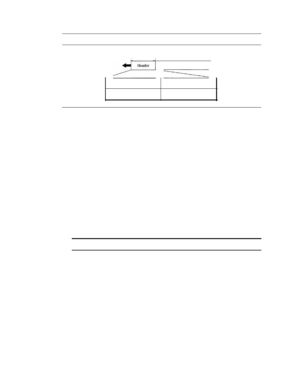
SECTION
23.2
USER DATAGRAM PROTOCOL (UDP)
711
Figure 23.9
User datagram format
8 bytes
I'
'I
Data
Source port number
16 bits
Total length
16 bits
Destination port number
16 bits
Checksum
16 bits
o
Destination port number.
This is the port number used by the process running on
the destination host.
It
is also 16 bits long.
If
the destination host is the server (a
client sending a request), the port number, in most cases, is a well-known port
number.
If
the destination host is the client (a server sending a response), the port
number, in most cases, is an ephemeral port number. In this case, the server copies
the ephemeral port number it has received in the request packet.
o
Length.
This is a 16-bit field that defines the total length of the user datagram,
header plus data. The 16 bits can define a total length of 0 to 65,535 bytes. How-
ever, the total length needs to be much less because a UDP user datagram is stored
in an IP datagram with a total length of 65,535 bytes.
The length field in a UDP user datagram is actually not necessary. A user
datagram is encapsulated in an IP datagram. There is a field in the IP datagram
that defines the total length. There is another field in the IP datagram that defines
the length of the header. So if we subtract the value of the second field from the
first, we can deduce the length of a UDP datagram that is encapsulated in an
IP datagram.
UDP length
=
IP length - IP header's length
However, the designers of the UDP protocol felt that it was more efficient for the
destination UDP to calculate the length of the data from the information provided
in the UDP user datagram rather than ask the IP software to supply this information.
We should remember that when the IP software delivers the UDP user datagram to
the UDP layer, it has already dropped the IP header.
o
Checksum.
This field is used to detect errors over the entire user datagram (header
plus data). The checksum is discussed next.
Checksum
We have already talked about the concept of the checksum and the way it is calculated
in Chapter 10. We have also shown how to calculate the checksum for the IP and ICMP
packet. We now show how this is done for UDP.
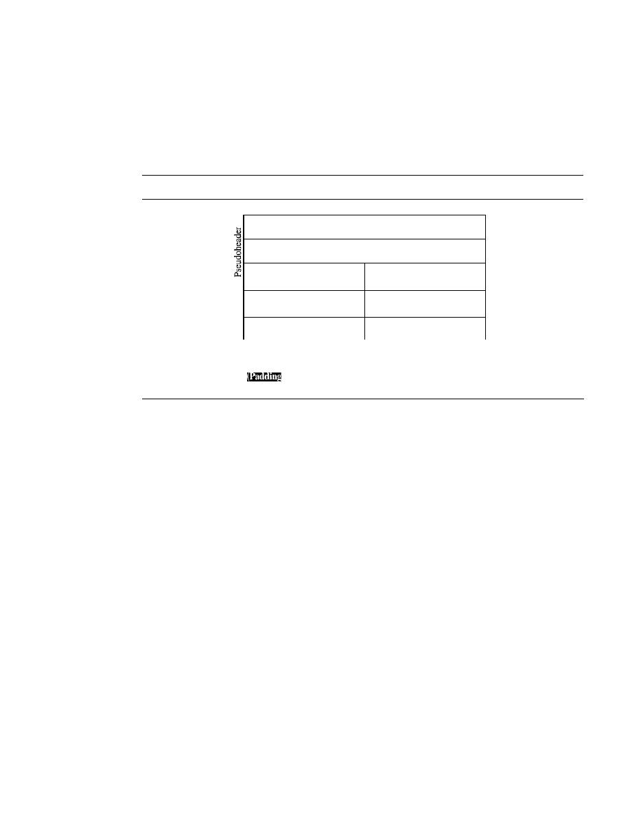
712
CHAPTER
23
PROCESS-TO-PROCESS DELIVERY: UDp, TCp, AND SCTP
The UDP checksum calculation is different from the one for IP and ICMP. Here
the checksum includes three sections: a pseudoheader, the UDP header, and the data
coming from the application layer.
The pseudoheader is the part of the header of the IP packet in which the user data-
gram is to be encapsulated with some fields filled with Os (see Figure 23.10).
Figure 23.10
Pseudoheader for checksum calculation
32-bit source IP address
32-bit destination IP address
AliOs
I
8-bit protocol
16-bit UDP total length
(17)
Source port address
Destination port address
16 bits
16 bits
UDP total length
Checksum
16 bits
16 bits
J)ata
must be added to make the data a multiple of 16 bits)
If
the checksum does not include the pseudoheader, a user datagram may arrive safe
and sound. However, if the IP header is corrupted, it may be delivered to the wrong host.
The protocol field is added to ensure that the packet belongs to UDP, and not
to other transport-layer protocols. We will see later that if a process can use either UDP
or TCP, the destination port number can be the same. The value of the protocol field
for UDP is 17.
If
this value is changed during transmission, the checksum calculation at
the receiver will detect it and UDP drops the packet.
It
is not delivered to the wrong
protocol.
Note the similarities between the pseudoheader fields and the last 12 bytes of the
IP header.
Example 23.2
Figure 23.11 shows the checksum calculation for a very small user datagram with only 7 bytes
of data. Because the number of bytes of data is odd, padding is added for checksum calcUlation.
The pseudoheader as well
as
the padding will be dropped when the user datagram is delivered
to IP.
Optional Use ofthe Checksum
The calculation of the checksum and its inclusion in a user datagram are optional.
If
the checksum is not calculated, the field is filled with 1s. Note that a calculated check-
sum can never be allIs because this implies that the sum is all Os, which is impossible
because it requires that the value of fields to be Os.
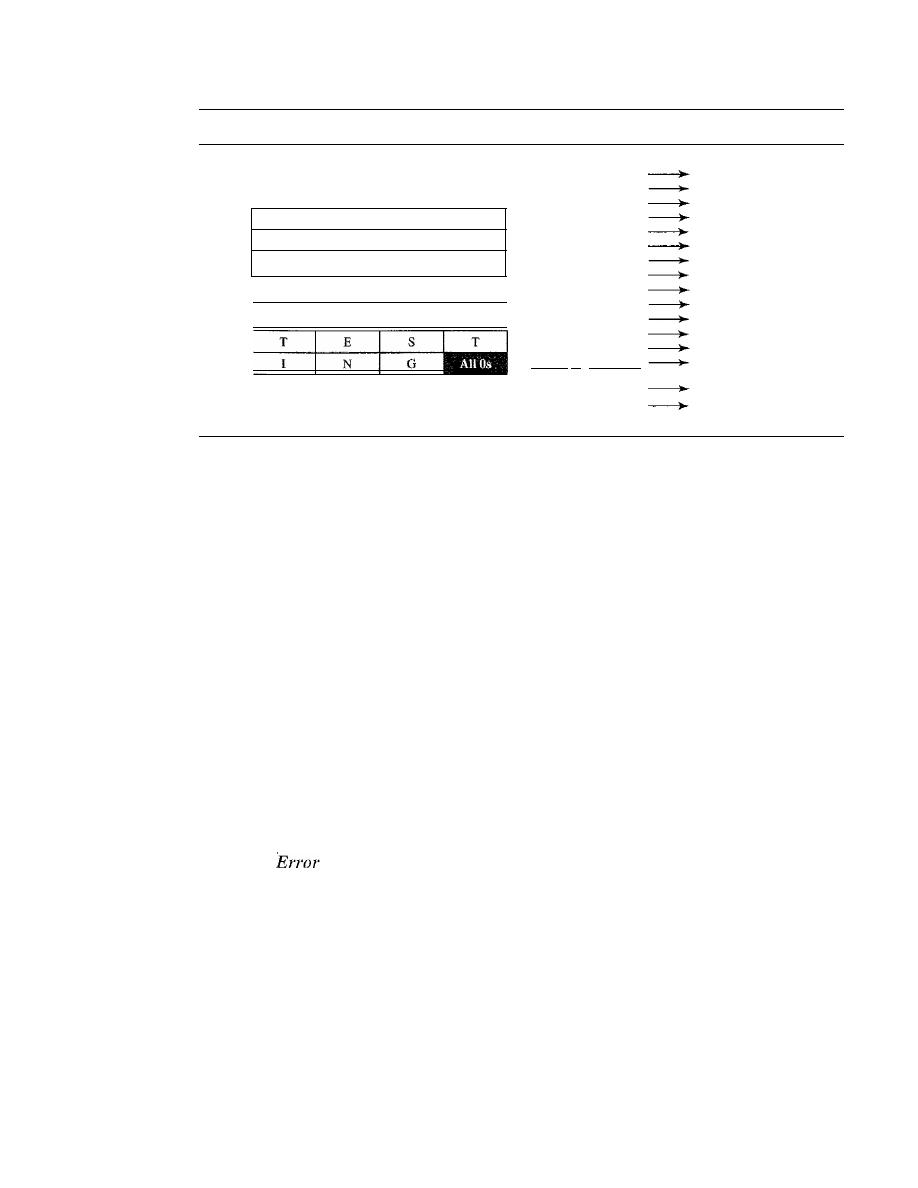
SECTION
23.2
USER DATAGRAM PROTOCOL (UDP)
713
Figure 23.11
Checksum calculation of a simple UDP user datagram
153.18.8.105
171.2.14.10
All Os
I
17
I
15
1087
15
13
All Os
10011001 00010010
153.18
00001000 01101001
8.105
10101011 0000001 0
171.2
00001110 00001010
14.10
00000000 00010001
o
and
17
00000000 00001111
15
00000100 00111111
1087
00000000 00001101
13
00000000 00001111
15
00000000 00000000
0
(checksum)
01010100 01000101
T and E
01010011 01010100
Sand
T
01001001 01001110
I
and N
010001 II 00000000
G and
0 (padding)
1O01O110 11101011
Sum
HUHIOOl
00010100
Checksum
UDP Operation
UDP uses concepts common to the transport layer. These concepts will be discussed
here briefly, and then expanded in the next section on the TCP protocol.
Connectionless Services
As mentioned previously, UDP provides a connectionless service. This means that each
user datagram sent by UDP is an independent datagram. There is no relationship
between the different user datagrams even if they are coming from the same source pro-
cess and going to the same destination program. The user datagrams are not numbered.
Also, there is no connection establishment and no connection termination, as is the case
for TCP. This means that each user datagram can travel on a different path.
One of the ramifications of being connectionless is that the process that uses UDP
cannot send a stream of data to UDP and expect UDP to chop them into different
related user datagrams. Instead each request must be small enough to fit into one user
datagram. Only those processes sending short messages should use UDP.
Flow and
Control
UDP is a very simple, unreliable transport protocol. There is no flow control and hence
no window mechanism. The receiver may overflow with incoming messages.
There is no error control mechanism in UDP except for the checksum. This means
that the sender does not know if a message has been lost or duplicated. When the receiver
detects an error through the checksum, the user datagram is silently discarded.
The lack of flow control and error control means that the process using UDP
should provide these mechanisms.
Encapsulation and Decapsulation
To send a message from one process to another, the UDP protocol encapsulates and
decapsulates messages in an IP datagram.
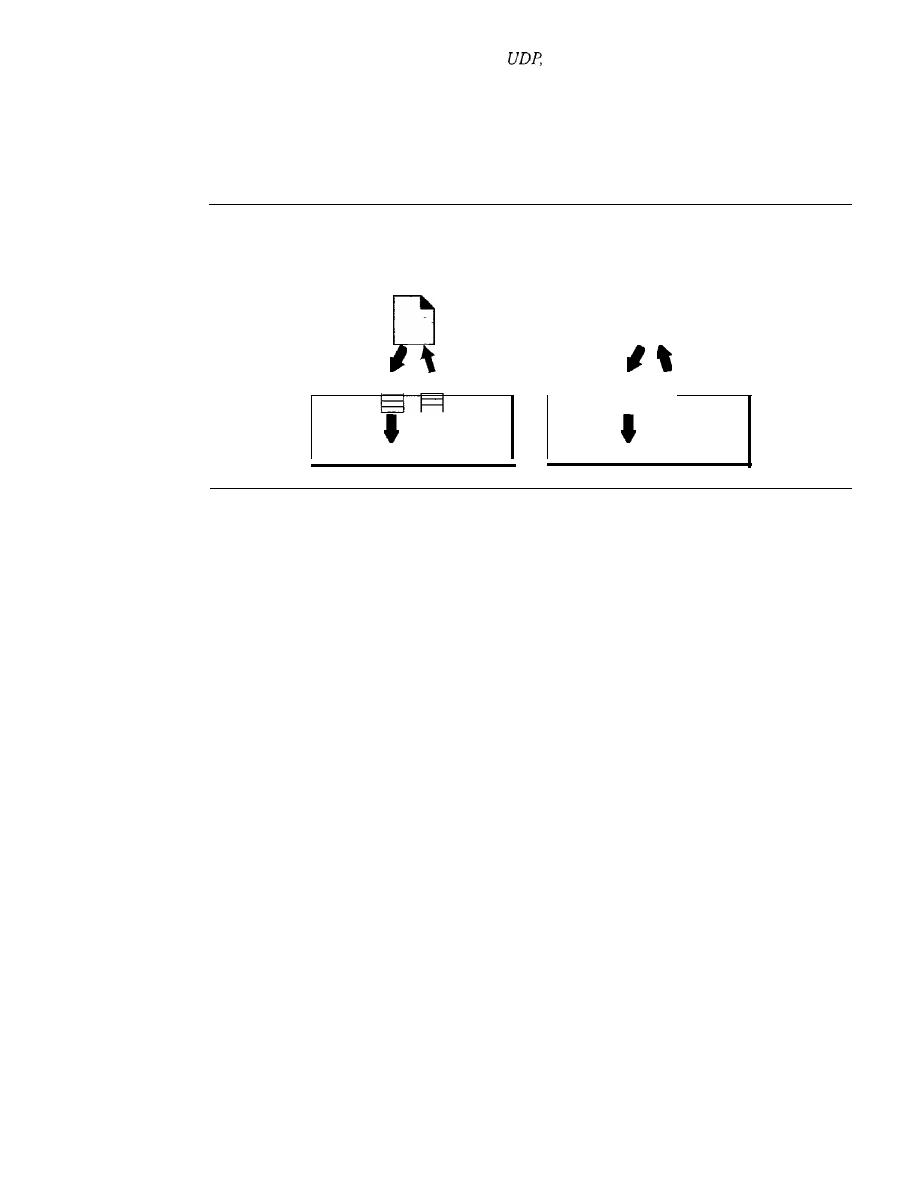
714
CHAPTER
23
PROCESS-TO-PROCESS DELIVERY:
TCp, AND SCTP
Queuing
We have talked about ports without discussing the actual implementation of them. In
UDP, queues are associated with ports (see Figure 23.12).
Figure 23.12
Queues in UDP
Daytime
Daytime
client
server
D
Outgoing
Incoming
Outgoing
Incoming
queue
queue
queue
queue
t
t
UDP
Port 52000
UDP
Port 13
At the client site, when a process starts, it requests a port number from the operating
system. Some implementations create both an incoming and an outgoing queue associated
with each process. Other implementations create only an incoming queue associated
with each process.
Note that even if a process wants to communicate with multiple processes, it
obtains only one port number and eventually one outgoing and one incoming queue.
The queues opened by the client are, in most cases, identified by ephemeral port numbers.
The queues function as long as the process is running. When the process terminates, the
queues are destroyed.
The client process can send messages to the outgoing queue by using the source
port number specified in the request. UDP removes the messages one by one and, after
adding the UDP header, delivers them to IP. An outgoing queue can overflow.
If
this
happens, the operating system can ask the client process to wait before sending any
more messages.
When a message arrives for a client, UDP checks to see if an incoming queue has
been created for the port number specified in the destination port number field of the
user datagram. If there is such a queue, UDP sends the received user datagram to the
end of the queue.
If
there is no such queue, UDP discards the user datagram and asks
the ICMP protocol to send a
port unreachable
message to the server. All the incoming
messages for one particular client program, whether coming from the same or a different
server, are sent to the same queue. An incoming queue can overflow.
If
this happens,
UDP drops the user datagram and asks for a port unreachable message to be sent to
the server.
At the server site, the mechanism of creating queues is different. In its simplest form,
a server asks for incoming and outgoing queues, using its well-known port, when it starts
running. The queues remain open as long as the server is running.
When a message arrives for a server, UDP checks to see if an incoming queue has
been created for the port number specified in the destination port number field of the user

SECTION
23.3
TCP
715
datagram. If there is such a queue, UDP sends the received user datagram to the end of
the queue.
If
there is no such queue, UDP discards the user datagram and asks the ICMP
protocol to send a port unreachable message to the client. All the incoming messages
for one particular server, whether coming from the same or a different client, are sent to
the same queue. An incoming queue can overflow.
If
this happens, UDP drops the user
datagram and asks for a port unreachable message to be sent to the client.
When a server wants to respond to a client, it sends messages to the outgoing queue,
using the source port number specified in the request. UDP removes the messages one
by one and, after adding the UDP header, delivers them to IP. An outgoing queue can
overflow.
If
this happens, the operating system asks the server to wait before sending
any more messages.
Use ofUDP
The following lists some uses of the UDP protocol:
o
UDP is suitable for a process that requires simple request-response communication
with little concern for flow and error control.
It
is not usually used for a process
such as FrP that needs to send bulk data (see Chapter 26).
o
UDP is suitable for a process with internal flow and error control mechanisms. For
example, the Trivial File Transfer Protocol (TFTP) process includes flow and error
control.
It
can easily use UDP.
o
UDP is a suitable transport protocol for multicasting. Multicasting capability is
embedded in the UDP software but not in the TCP software.
o
UDP is used for management processes such as SNMP (see Chapter 28).
o
UDP is used for some route updating protocols such as Routing Information Protocol
(RIP) (see Chapter 22).
23.3
TCP
The second transport layer protocol we discuss in this chapter is called Transmission
Control Protocol (TCP). TCP, like UDP, is a process-to-process (program-to-program)
protocol. TCP, therefore, like UDP, uses port numbers. Unlike UDP, TCP is a connection-
oriented protocol; it creates a virtual connection between two TCPs to send data. In
addition, TCP uses flow and error control mechanisms at the transport level.
In brief, TCP is called a connection-oriented, reliable transport protocol.
It
adds
connection-oriented and reliability features to the services of IP.
TCP Services
Before we discuss TCP in detail, let us explain the services offered by TCP to the pro-
cesses at the application layer.
Process-to-Process Communication
Like UDP, TCP provides process-to-process communication using port numbers. Table 23.2
lists some well-known port numbers used by TCP.
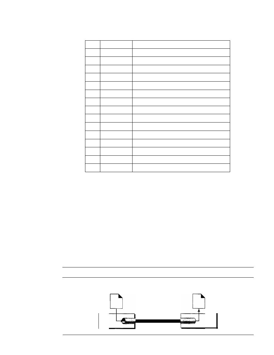
716
CHAPTER
23
PROCESS-TO-PROCESS DELIVERY: UDp, TCP, AND SCTP
Table 23.2
Well-known ports used by TCP
Port
Protocol
Description
7
Echo
Echoes a received datagram back to the sender
9
Discard
Discards any datagram that is received
11
Users
Active users
13
Daytime
Returns the date and the time
17
Quote
Returns a quote of the day
19
Chargen
Returns a string of characters
20
FIP, Data
File Transfer Protocol (data connection)
21
FIP, Control
File Transfer Protocol (control connection)
23
TELNET
Tenninal Network
25
SMTP
Simple Mail Transfer Protocol
53
DNS
Domain Name Server
67
BOOTP
Bootstrap Protocol
79
Finger
Finger
80
HTTP
Hypertext Transfer Protocol
111
RPC
Remote Procedure Call
Stream Delivery Service
TCP, unlike UDP, is a stream-oriented protocol. In UDP, a process (an application pro-
gram) sends messages, with predefined boundaries, to UDP for delivery. UDP adds its
own header to each of these messages and delivers them to IP for transmission. Each
message from the process is calIed a user datagram and becomes, eventually, one IP
datagram. Neither IP nor UDP recognizes any relationship between the datagrams.
TCP, on the other hand, allows the sending process to deliver data as a stream of
bytes and allows the receiving process to obtain data as a stream of bytes. TCP creates
an environment in which the two processes seem to be connected by an imaginary "tube"
that carries their data across the Internet. This imaginary environment is depicted in
Figure 23.13. The sending process produces (writes to) the stream of bytes, and the
receiving process consumes (reads from) them.
Figure 23.13
Stream delivery
Sending
process
Receiving
process
TCP
TCP
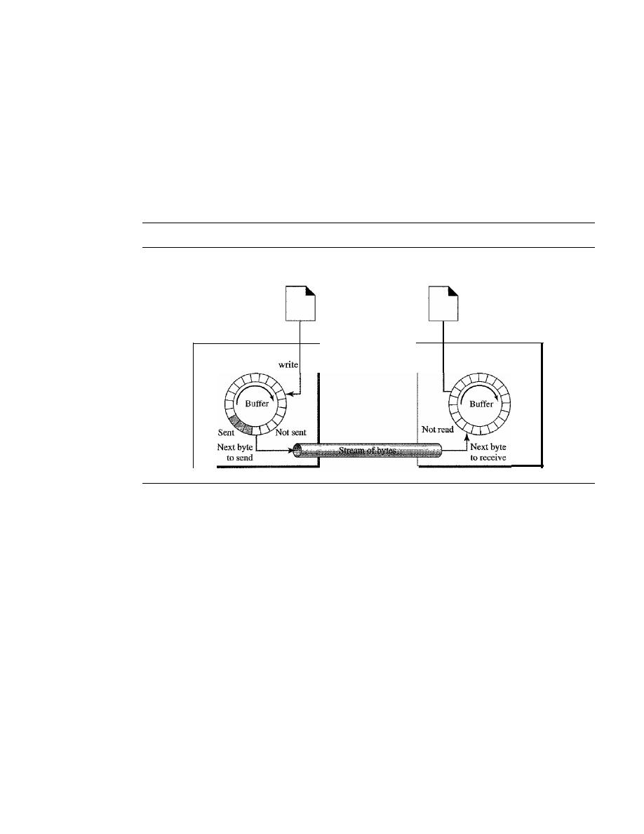
SECTION
23.3
TCP
717
Sending and Receiving Buffers
Because the sending and the receiving processes may
not write or read data at the same speed, TCP needs buffers for storage. There are two
buffers, the sending buffer and the receiving buffer, one for each direction. (We will see
later that these buffers are also necessary for flow and error control mechanisms used
by TCP.) One way to implement a buffer is to use a circular array of I-byte locations as
shown in Figure 23.14. For simplicity, we have shown two buffers of 20 bytes each;
normally the buffers are hundreds or thousands of bytes, depending on the implemen-
tation. We also show the buffers as the same size, which is not always the case.
Figure 23.14
Sending and receiving buffers
Sending
process
TCP
Next byte
to
Receiving
process
Next byte
to read
TCP
Figure 23.14 shows the movement of the data in one direction. At the sending site,
the buffer has three types of chambers. The white section contains empty chambers that
can be filled by the sending process (producer). The gray area holds bytes that have
been sent but not yet acknowledged. TCP keeps these bytes in the buffer until it receives
an acknowledgment. The colored area contains bytes to be sent by the sending TCP.
However, as we will see later in this chapter, TCP may be able to send only part of this
colored section. This could be due to the slowness of the receiving process or perhaps
to congestion in the network. Also note that after the bytes in the gray chambers are
acknowledged, the chambers are recycled and available for use by the sending process.
This is why we show a circular buffer.
The operation of the buffer at the receiver site is simpler. The circular buffer is
divided into two areas (shown as white and colored). The white area contains empty
chambers to be filled by bytes received from the network. The colored sections contain
received bytes that can be read by the receiving process. When a byte is read by the
receiving process, the chamber is recycled and added to the pool of empty chambers.
Segments
Although buffering handles the disparity between the speed of the producing
and consuming processes, we need one more step before we can send data. The IP layer,
as a service provider for TCP, needs to send data in packets, not as a stream of bytes. At
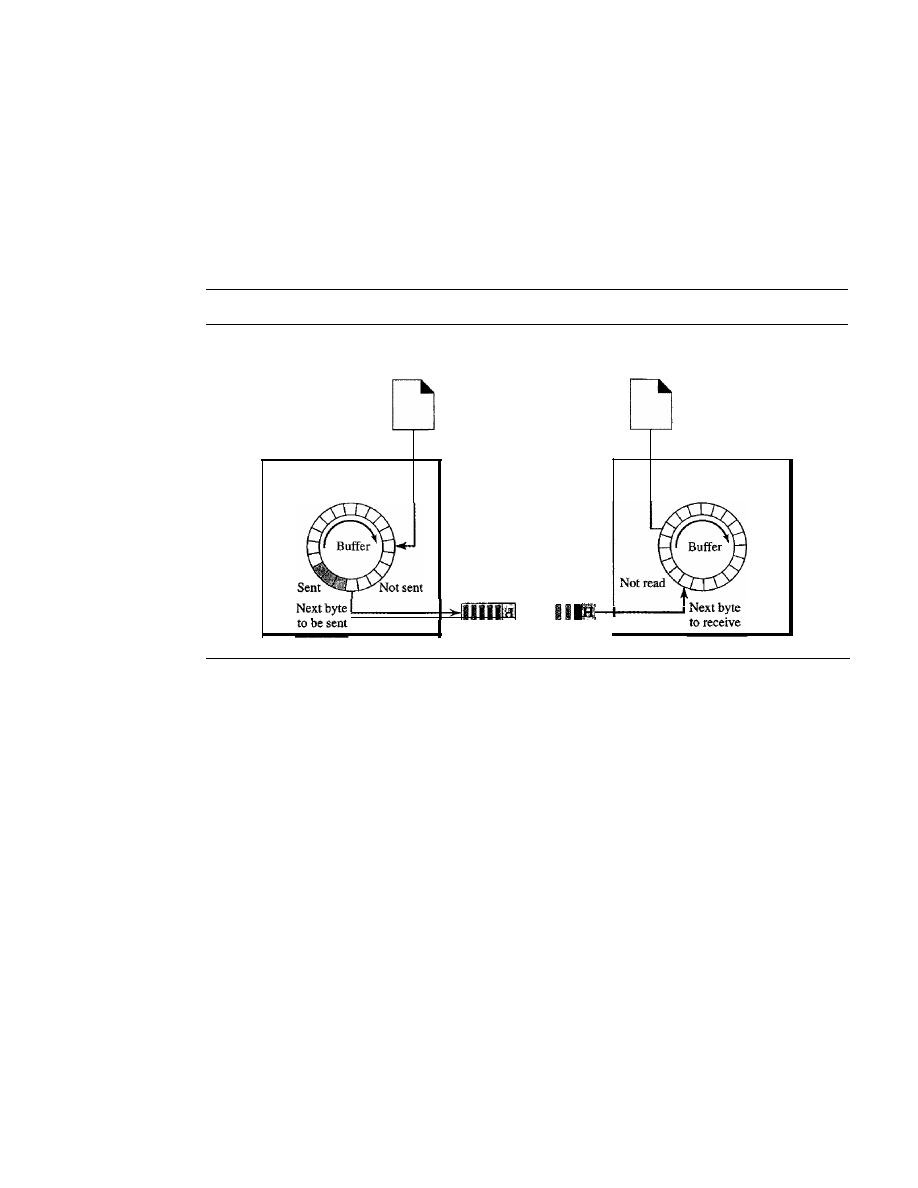
718
CHAPTER
23
PROCESS-TO-PROCESS DELIVERY: UDp, TCp, AND SCTP
the transport layer, TCP groups a number of bytes together into a packet called a segment.
TCP adds a header to each segment (for control purposes) and delivers the segment to the
IP layer for transmission. The segments are encapsulated in IP datagrams and transmit-
ted. This entire operation is transparent to the receiving process. Later we will see that
segments may be received out of order, lost, or corrupted and resent. All these are handled
by TCP with the receiving process unaware of any activities. Figure 23.15 shows how
segments are created from the bytes in the buffers.
Figure 23.15
TCP segments
Sending
process
Receiving
process
TCP
TCP
Next byte
to accept
Next byte
to deliver
Segment
1
SegmentN
•••
Note that the segments are not necessarily the same size. In Figure 23.15, for sim-
plicity, we show one segment carrying 3 bytes and the other carrying 5 bytes. In reality,
segments carry hundreds, if not thousands, of bytes.
Full-Duplex Communication
TCP offers full-duplex service, in which data can flow in both directions at the same time.
Each TCP then has a sending and receiving buffer, and segments move in both directions.
Connection-Oriented Service
TCP, unlike UDP, is a connection-oriented protocol. When a process at site A wants to
send and receive data from another process at site B, the following occurs:
1. The two TCPs establish a connection between them.
2. Data are exchanged in both directions.
3. The connection is terminated.
Note that this is a virtual connection, not a physical connection. The TCP segment is
encapsulated in an IP datagram and can be sent out of order, or lost, or corrupted, and then
resent. Each may use a different path to reach the destination. There is no physical connec-
tion. TCP creates a stream-oriented environment in which it accepts the responsibility of

SECT/ON
23.3
TCP
719
delivering the bytes in order to the other site. The situation is similar to creating a bridge
that spans multiple islands and passing all the bytes from one island to another in one
single connection. We will discuss this feature later in the chapter.
Reliable Service
TCP is a reliable transport protocol.
It
uses an acknowledgment mechanism to check
the safe and sound arrival of data. We will discuss this feature further in the section on
error control.
TCP Features
To provide the services mentioned in the previous section, TCP has several features that
are briefly summarized in this section and discussed later in detail.
Numbering System
Although the TCP software keeps track of the segments being transmitted or received,
there is no field for a segment number value in the segment header. Instead, there are
two fields called the
sequence number
and the
acknowledgment number.
These two
fields refer to the byte number and not the segment number.
Byte Number
TCP numbers all data bytes that are transmitted in a connection. Number-
ing is independent in each direction. When TCP receives bytes of data from a process, it
stores them in the sending buffer and numbers them. The numbering does not necessarily
start from O. Instead, TCP generates a random number between 0 and 2
32
-
1 for the num-
ber of the first byte. For example, if the random number happens to be 1057 and the total
data to be sent are 6000 bytes, the bytes are numbered from 1057 to 7056. We will see that
byte numbering is used for flow and error control.
The bytes of data being transferred in each connection are numbered by TCP.
The numbering starts with a randomly generated number.
Sequence Number
After the bytes have been numbered, TCP assigns a sequence
number to each segment that is being sent. The sequence number for each segment is
the number of the first byte carried in that segment.
Example 23.3
Suppose a TCP connection is transferring a file of 5000 bytes. The first byte is numbered 1O,00l.
What are the sequence numbers for each segment if data are sent in five segments, each carrying
1000 bytes?
Solution
The following shows the sequence number for each segment:
Segment 1
Sequence Number: 10,001 (range: 10,001 to 11,(00)
Segment 2
Sequence Number: 11,001 (range: 11,001 to 12,000)
Segment 3
Sequence Number: 12,001 (range: 12,001 to 13,000)
Segment 4
Sequence Number: 13,001 (range: 13,001
to
14,000)
Segment 5
Sequence Number: 14,001 (range: 14,001 to 15,000)

720
CHAPTER
23
PROCESS- TO-PROCESS DEliVERY: UDp, TCP, AND SCTP
The value in the sequence number field of a segment defines the
number of the first data byte contained in that segment.
When a segment carries a combination of data and control information (piggy-
backing), it uses a sequence number.
If
a segment does not carry user data, it does not
logically define a sequence number. The field is there, but the value is not valid. However,
some segments, when carrying only control information, need a sequence number to
allow an acknowledgment from the receiver. These segments are used for connection
establishment, termination, or abortion. Each of these segments consumes one sequence
number as though it carried 1 byte, but there are no actual data. If the randomly generated
sequence number is
x,
the first data byte is numbered
x
+
1. The byte
x
is considered a
phony byte that is used for a control segment to open a connection, as we will see shortly.
Acknowledgment Number
As we discussed previously, communication in TCP is full
duplex; when a connection is established, both parties can send and receive data at the
same time. Each party numbers the bytes, usually with a different starting byte number.
The sequence number in each direction shows the number of the first byte carried by
the segment. Each party also uses an acknowledgment number to confirm the bytes it has
received. However, the acknowledgment number defines the number of the next byte
that the party expects to receive.
In addition, the acknowledgment number is cumula-
tive, which means that the party takes the number of the last byte that it has received,
safe and sound, adds I to it, and announces this sum as the acknowledgment number.
The term cumulative here means that if a party uses 5643 as an acknowledgment number,
it
has received all bytes from the beginning up to 5642. Note that this does not mean
that the party has received 5642 bytes because the first byte number does not have to start
from O.
The value of the acknowledgment field in a segment defines
the number of the next byte a party expects to receive.
The acknowledgment number is cumulative.
Flow Control
TCP, unlike UDP, provides flow control. The receiver of the data controls the amount of
data that are to be sent by the sender. This is done to prevent the receiver from being over-
whelmed with data. The numbering system allows TCP to use a byte-oriented flow control.
Error Control
To provide reliable service, TCP implements an error control mechanism. Although
error control considers a segment as the unit of data for error detection (loss or corrupted
segments), error control is byte-oriented, as we will see later.
Congestion Control
TCP, unlike UDP, takes into account congestion in the network. The amount of data sent
by a sender is not only controlled by the receiver (flow control), but is also detennined
by the level of congestion in the network.
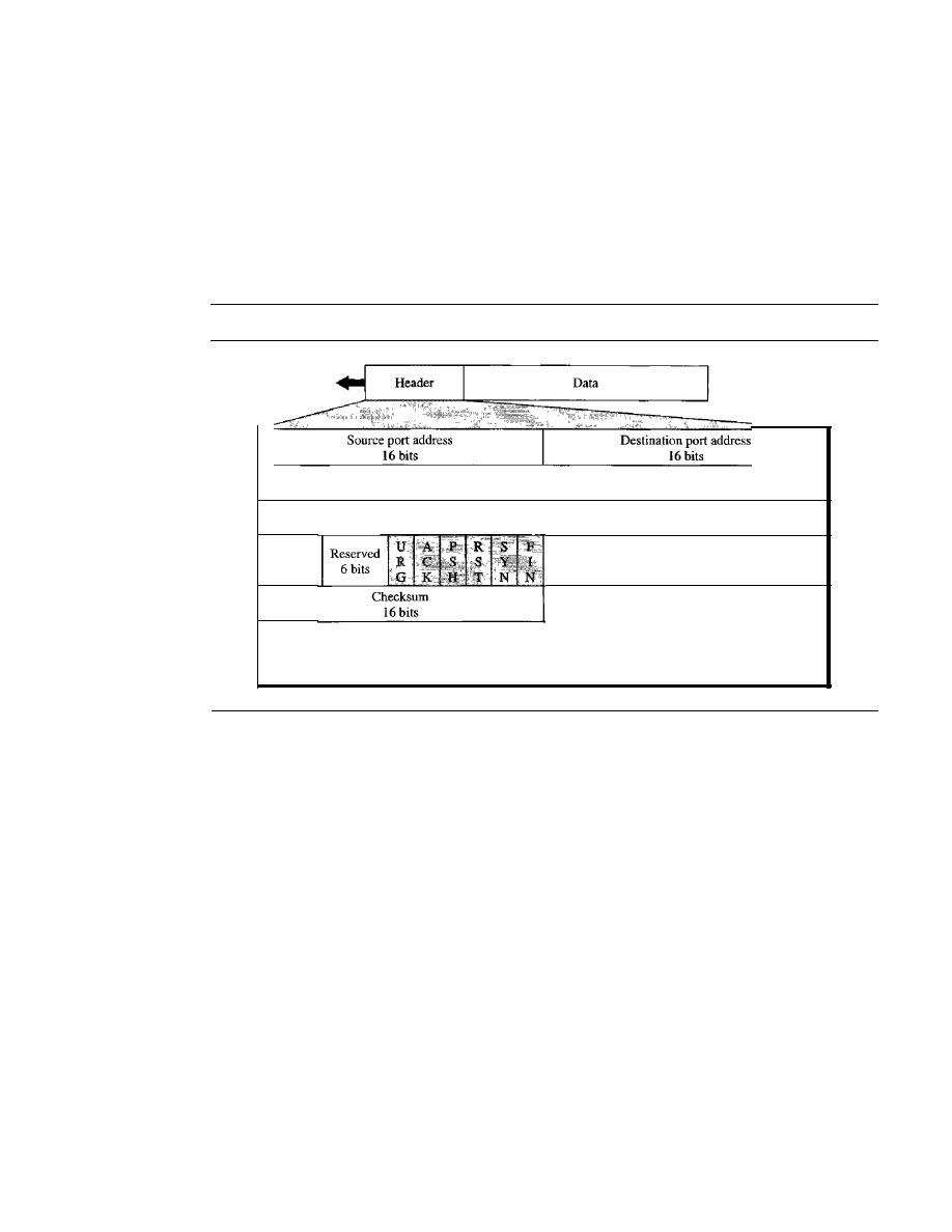
SECTION
23.3
TCP
721
Segment
Before we discuss TCP in greater detail, let us discuss the TCP packets themselves. A
packet in TCP is called a
segment.
Format
The format of a segment is shown in Figure 23.16.
Figure 23.16
TCP segment format
Sequence number
32 bits
Acknowledgment number
32 bits
HLEN
4 bits
Options and Padding
Window size
16
bits
Urgent pointer
16
bits
The segment consists of a 20- to 60-byte header, followed by data from the appli-
cation program. The header is 20 bytes if there are no options and up to 60 bytes if
it
contains options. We will discuss some of the header fields in this section. The meaning
and purpose of these will become clearer as we proceed through the chapter.
o
Source port address.
This is a 16-bit field that defines the port number of the
application program in the host that is sending the segment. This serves the same
purpose as the source port address in the UDP header.
o
Destination port address.
This is a 16-bit field that defines the port number of the
application program in the host that is receiving the segment. This serves the same
purpose as the destination port address in the UDP header.
o
Sequence number.
This 32-bit field defines the number assigned to the first byte of
data contained
in
this segment. As we said before, TCP is a stream transport protocol.
To ensure connectivity, each byte to be transmitted is numbered. The sequence number
tells the destination which byte in this sequence comprises the first byte in the seg-
ment. During connection establishment, each party uses a random number generator to
create an
initial sequence number (ISN),
which is usually different
in
each direction.
o
Acknowledgment number.
This 32-bit field defines the byte number that the
receiver of the segment is expecting to receive from the other party.
If
the receiver

722
CHAPTER
23
PROCESS-TO-PROCESS DELIVERY: UDp, TCp, AND SCTP
of the segment has successfully received byte number x from the other party, it
defines
x
+
I as the acknowledgment number. Acknowledgment and data can be
piggybacked together.
D
Header length.
This 4-bit field indicates the number of 4-byte words in the TCP
header. The length of the header can be between 20 and 60 bytes. Therefore, the
value of this field can be between 5 (5 x 4
=
20) and 15 (15 x 4
=
60).
D
Reserved.
This is a 6-bit field reserved for future use.
D
Control.
This field defines 6 different control bits or flags as shown in Figure 23.17.
One or more of these bits can be set at a time.
Figure 23.17
Control field
RST
RST: Reset the connection
SYN: Synchronize sequence numbers
FIN: Terminate the connection
PSH
ACK
URG: Urgent pointer is valid
ACK:
Acknowledgment is valid
PSH: Request for push
URG
SYN
FIN
I
_ _ _ _
_
These bits enable flow control, connection establishment and termination, connection
abortion, and the mode of data transfer in TCP. A brief description of each bit is shown in
Table 23.3. We will discuss them further when we study the detailed operation of TCP
later in the chapter.
Table 23.3
Description offlags in the control field
Flag
Description
URG
The value of the urgent pointer field is valid.
ACK
The value of the acknowledgment field is valid.
PSH
Push the data.
RST
Reset the connection.
SYN
Synchronize sequence numbers during connection.
FIN
Terminate the connection.
D
Window size.
This field defines the size of the window, in bytes, that the other
party must maintain. Note that the length of this field is 16 bits, which means that
the maximum size of the window is 65,535 bytes. This value is normally referred
to as the receiving window (rwnd) and is determined by the receiver. The sender
must obey the dictation of the receiver in this case.
D
Checksum.
This 16-bit field contains the checksum. The calculation of the check-
sum for TCP follows the same procedure as the one described for UDP. However, the
inclusion of the checksum in the UDP datagram is optional, whereas the inclusion
of the checksum for TCP is mandatory. The same pseudoheader, serving the same

SECTION 23.3
TCP
723
purpose, is added to the segment. For the TCP pseudoheader, the value for the pro-
tocol field is 6.
o
Urgent pointer. This l6-bit field, which is valid only if the urgent flag is set, is
used when the segment contains urgent data.
It
defines the number that must be
added to the sequence number to obtain the number of the last urgent byte in the
data section of the segment. This will be discussed later in this chapter.
o
Options. There can be up to 40 bytes of optional information in the TCP header.
We will not discuss these options here; please refer to the reference list for more
information.
A TCP Connection
TCP is connection-oriented. A connection-oriented transport protocol establishes a
virtual path between the source and destination. All the segments belonging to a mes-
sage are then sent over this virtual path. Using a single virtual pathway for the entire
message facilitates the acknowledgment process as well as retransmission of damaged
or lost frames. You may wonder how TCP, which uses the services of IP, a connection-
less protocol, can be connection-oriented. The point is that a TCP connection is virtual,
not physical. TCP operates at a higher level. TCP uses the services of IP to deliver indi-
vidual segments to the receiver, but it controls the connection itself.
If
a segment is lost
or corrupted, it is retransmitted. Unlike TCP, IP is unaware of this retransmission. If a
segment arrives out of order, TCP holds it until the missing segments arrive; IP is
unaware of this reordering.
In TCP, connection-oriented transmission requires three phases: connection estab-
lishment, data transfer, and connection termination.
Connection Establishment
TCP transmits data in full-duplex mode. When two TCPs in two machines are con-
nected, they are able to send segments to each other simultaneously. This implies that
each party must initialize communication and get approval from the other party before
any data are transferred.
Three-Way Handshaking
The connection establishment in TCP is called three-
way handshaking. In our example, an application program, called the client, wants to
make a connection with another application program, called the server, using TCP as
the transport layer protocol.
The process starts with the server. The server program tells its TCP that it is ready
to accept a connection. This is called a request for a
passive open.
Although the server
TCP is ready to accept any connection from any machine in the world, it cannot make
the connection itself.
The client program issues a request for an
active open.
A client that wishes to con-
nect to an open server tells its TCP that it needs to be connected to that particular
server. TCP can now start the three-way handshaking process as shown in Figure 23.18.
To show the process, we use two time lines: one at each site. Each segment has values
for all its header fields and perhaps for some of its option fields, too. However, we show
only the few fields necessary to understand each phase. We show the sequence number,
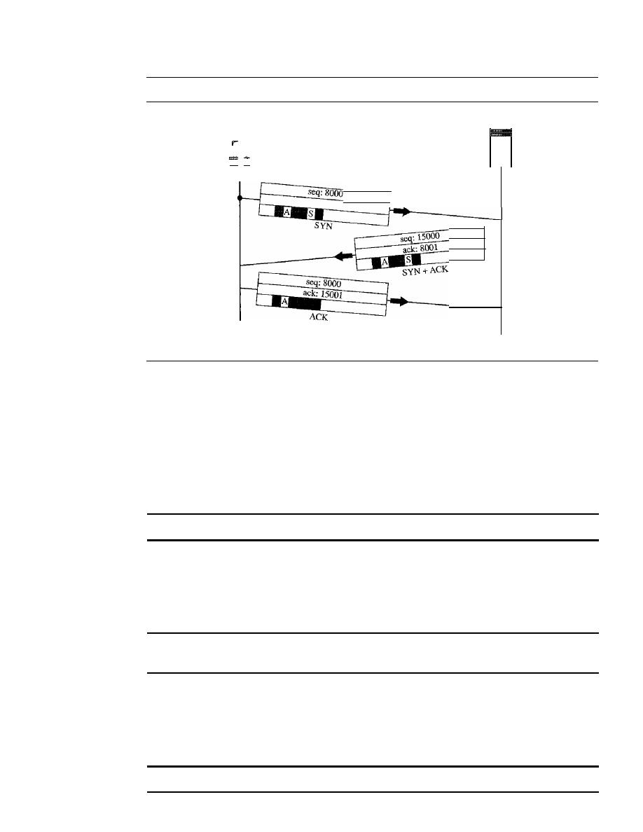
724
CHAPTER
23
PROCESS-TO-PROCESS DELIVERY: UDp, TCP, AND SCTP
Figure 23.18
Connection establishment using three-way handshaking
Client
A: ACK
flag
S: SYN flag
Server
Active
open
Time
Passive
open
Time
the acknowledgment number, the control flags (only those that are set), and the window
size, if not empty. The three steps in this phase are as follows.
1. The client sends the first segment, a SYN segment, in which only the SYN flag is set.
This segment is for synchronization of sequence numbers.
It
consumes one sequence
number. When the data transfer starts, the sequence number is incremented by 1. We
can say that the SYN segment carries no real data, but we can
think
of it as containing
1 imaginary byte.
A SYN segment cannot carry data, but it consumes one sequence number.
2. The server sends the second segment, a SYN
+
ACK segment, with 2 flag bits set:
SYN and ACK. This segment has a dual purpose.
It
is a SYN segment for commu-
nication in the other direction and serves as the acknowledgment for the SYN
segment.
It
consumes one sequence number.
A SYN
+
ACK segment cannot carry data,
but does consume one sequence number.
3. The client sends the third segment. This is just an ACK segment.
It
acknowledges
the receipt of the second segment with the ACK flag and acknowledgment number
field. Note that the sequence number in this segment is the same as the one in the
SYN segment; the ACK segment does not consume any sequence numbers.
An ACK segment,
if
carrying no data, consumes no sequence number.

SECTION
23.3
TCP
725
Simultaneous Open
A rare situation, called a simultaneous open, may occur when
both processes issue an active open. In this case, both TCPs transmit a SYN
+
ACK
segment to each other, and one single connection is established between them.
SYN Flooding Attack
The connection establishment procedure in TCP is susceptible
to a serious security problem called the SYN flooding attack. This happens when a mali-
cious attacker sends a large number of SYN segments to a server, pretending that each
of them is corning from a different client by faking the source IP addresses in the data-
grams. The server, assuming that the clients are issuing an active open, allocates the
necessary resources, such as creating communication tables and setting timers. The
TCP server then sends the SYN
+
ACK segments to the fake clients, which are lost. Dur-
ing this time, however, a lot of resources are occupied without being used.
If,
during this
short time, the number of SYN segments is large, the server eventually runs out of
resources and may crash. This SYN flooding attack belongs to a type of security attack
known as a denial-of-service attack, in which an attacker monopolizes a system with
so many service requests that the system collapses and denies service to every request.
Some implementations of TCP have strategies to alleviate the effects of a SYN
attack. Some have imposed a limit on connection requests during a specified period of
time. Others filter out datagrams coming from unwanted source addresses. One recent
strategy is to postpone resource allocation until the entire connection is set up, using
what is called a cookie. SCTP, the new transport layer protocol that we discuss in the
next section, uses this strategy.
Data Transfer
After connection is established, bidirectional data transfer can take place. The client
and server can both send data and acknowledgments. We will study the rules of
acknowledgment later in the chapter; for the moment, it is enough to know that data
traveling in the same direction as an acknowledgment are carried on the same seg-
ment. The acknowledgment is piggybacked with the data. Figure 23.19 shows an example.
In this example, after connection is established (not shown in the figure), the client
sends 2000 bytes of data in two segments. The server then sends 2000 bytes in one seg-
ment. The client sends one more segment. The first three segments carry both data and
acknowledgment, but the last segment carries only an acknowledgment because there
are no more data to be sent. Note the values of the sequence and acknowledgment
numbers. The data segments sent by the client have the PSH (push) flag set so that the
server TCP knows to deliver data to the server process as soon as they are received.
We discuss the use of this flag in greater detail later. The segment from the server, on
the other hand, does not set the push flag. Most TCP implementations have the option
to set or not set this flag.
Pushing Data
We saw that the sending TCP uses a buffer to store the stream of data
coming from the sending application program. The sending TCP can select the segment
size. The receiving TCP also buffers the data when they arrive and delivers them to the
application program when the application program is ready or when it is convenient for
the receiving TCP. This type of flexibility increases the efficiency of TCP.
However, on occasion the application program has no need for this flexibility_ For
example, consider an application program that communicates interactively with another
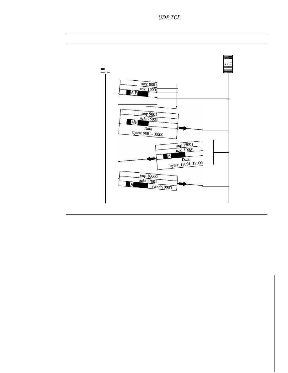
726
CHAPTER
23
PROCESS-TO-PROCESS DELIVERY:
AND SCTP
Figure 23.19
Data transfer
Server
Client
A: ACKflag
P: PSH flag
-
Data
bytes:
8001-9000
Time
Time
application program on the other end. The application program on one site wants to
send a keystroke to the application at the other site and receive an immediate response.
Delayed transmission and delayed delivery of data may not be acceptable by the applica-
tion program.
TCP can handle such a situation. The application program at the sending site can
request a push operation. This means that the sending TCP must not wait for the window
to be filled.
It
must create a segment and send it immediately. The sending TCP must
also set the push bit (PSH) to let the receiving TCP know that the segment includes data
that must be delivered to the receiving application program as soon as possible and not
to wait for more data to come.
Although the push operation can be requested by the application program, most
current implementations ignore such requests. TCP can choose whether or not to use
this feature.
Urgent Data
TCP is a stream-oriented protocol. This means that the data are presented
from the application program to TCP as a stream of bytes. Each byte of data has a posi-
tion in the stream. However, on occasion an application program needs to send urgent
bytes. This means that the sending application program wants a piece of data to be read
out of order by the receiving application program. As an example, suppose that the sending
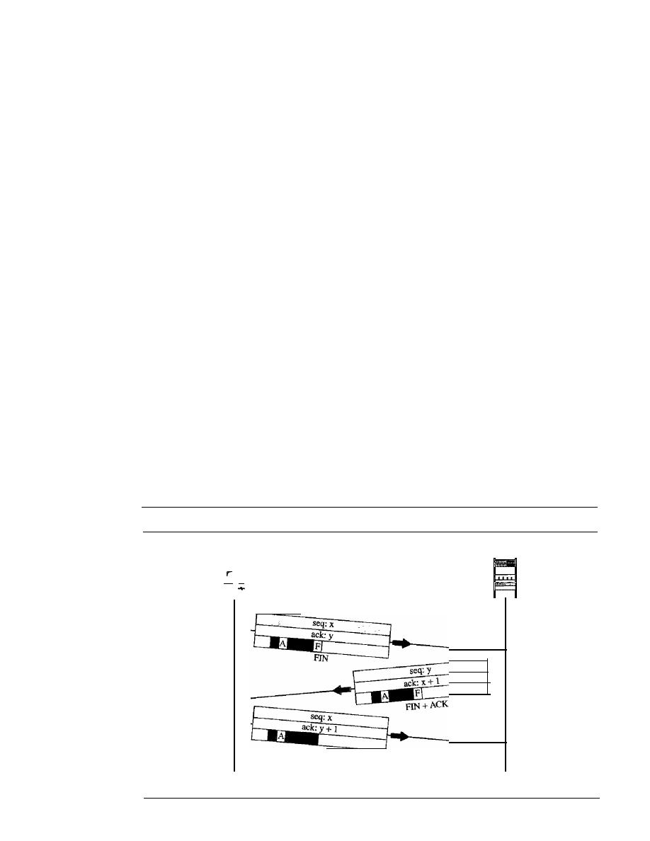
SECTION
23.3
TCP
727
application program is sending data to be processed by the receiving application
program. When the result of processing comes back, the sending application program
finds that everything is wrong.
It
wants to abort the process, but it has already sent a huge
amount of data.
If
it issues an abort command (control
+
C), these two characters will be
stored at the end of the receiving TCP buffer.
It
will be delivered to the receiving appli-
cation program after all the data have been processed.
The solution is to send a segment with the URG bit set. The sending application
program tells the sending TCP that the piece of data is urgent. The sending TCP creates
a segment and inserts the urgent data at the beginning of the segment. The rest of the
segment can contain normal data from the buffer. The urgent pointer field in the header
defines the end of the urgent data and the start of normal data.
When the receiving TCP receives a segment with the URG bit set, it extracts the
urgent data from the segment, using the value of the urgent pointer, and delivers them,
out of order, to the receiving application program.
Connection Termination
Any of the two parties involved in exchanging data (client or server) can close the connec-
tion, although it is usually initiated by the client. Most implementations today allow two
options for connection termination: three-way handshaking and four-way handshaking
with a half-close option.
Three-Way Handshaking
Most implementations today allow
three-way handshaking
for connection termination as shown in Figure 23.20.
1. In a normal situation, the client TCP, after receiving a close command from the
client process, sends the first segment, a FIN segment in which the FIN flag is set.
Note that a FIN segment can include the last chunk of data sent by the client, or it
Figure 23.20
Connection termination using three-way handshaking
Client
_
Active
close
Time
A: ACK flag
F: FIN
flag
ACK
Server
-
Passive
close
Time

728
CHAPTER
23
PROCESS-TO-PROCESS DELIVERY: UDp, TCp, AND SCTP
can be just a control segment as shown in Figure 23.20. If it is only a control seg-
ment, it consumes only one sequence number.
The FIN segment consumes one sequence number ifit does not carry data.
2. The server TCP, after receiving the FIN segment, informs its process of the situa-
tion and sends the second segment, a FIN
+
ACK segment, to confirm the receipt
of the FIN segment from the client and at the same time to announce the closing of
the connection in the other direction. This segment can also contain the last chunk
of data from the server. If it does not carry data, it consumes only one sequence
number.
The FIN
+
ACK segment consumes one sequence
number if it does not carry data.
3. The client TCP sends the last segment, an ACK segment, to confirm the receipt of
the FIN segment from the TCP server. This segment contains the acknowledgment
number, which is 1 plus the sequence number received in the FIN segment from
the server. This segment cannot carry data and consumes no sequence numbers.
Half-Close
In TCP, one end can stop sending data while still receiving data. This is
called a half-close. Although either end can issue a half-close, it is normally initiated by
the client. It can occur when the server needs all the data before processing can begin. A
good example is sorting. When the client sends data to the server to be sorted, the server
needs to receive all the data before sorting can start. This means the client, after sending
all the data, can close the connection in the outbound direction. However, the inbound
direction must remain open to receive the sorted data. The server, after receiving the
data, still needs time for sorting; its outbound direction must remain open.
Figure 23.21 shows an example of a half-close. The client half-closes the connection
by sending a FIN segment. The server accepts the half-close by sending the ACK segment.
The data transfer from the client to the server stops. The server, however, can still send
data. When the server has sent all the processed data, it sends a FIN segment, which is
acknowledged by an ACK from the client.
After half-closing of the connection, data can travel from the server to the client
and acknowledgments can travel from the client to the server. The client cannot send any
more data to the server. Note the sequence numbers we have used. The second segment
(ACK) consumes no sequence number. Although the client has received sequence number
y -
1 and is expecting
y,
the server sequence number is still
y -
1. When the connection
finally closes, the sequence number of the last ACK segment is still
x,
because no
sequence numbers are consumed during data transfer in that direction.
Flow Control
TCP uses a sliding window, as discussed in Chapter 11, to handle flow control. The
sliding window protocol used by TCP, however, is something between the
Go-Back-N
and Selective Repeat sliding window. The sliding window protocol in TCP looks like
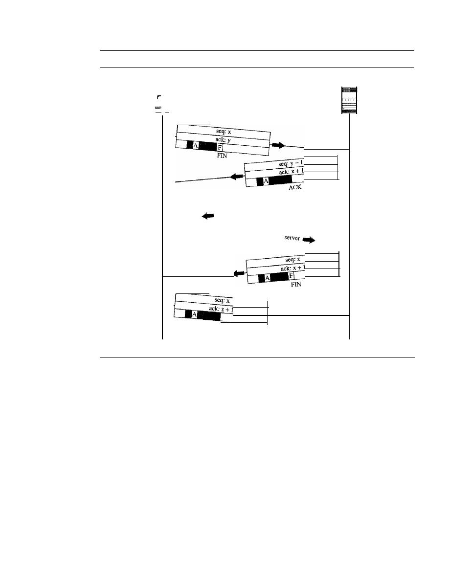
SECTION
23.3
TCP
729
Figure 23.21
Half-close
Server
Client
-
Active
close
Time
A: ACKfiag
F: FIN
flag
f
server to client
Data segments rom
ACknoWled
gments from client to
ACK
Passive
close
Time
the Go-Back-N protocol because
it
does not use NAKs; it looks like Selective Repeat
because the receiver holds the out-of-order segments until the missing ones arrive. There
are two big differences between this sliding window and the one we used at the data
link layer. First, the sliding window ofTCP is byte-oriented; the one we discussed in the
data link layer is frame-oriented. Second, the TCP's sliding window is of variable size;
the one we discussed in the data link layer was of fixed size.
Figure 23.22 shows the sliding window in TCP. The window spans a portion of the
buffer containing bytes received from the process. The bytes inside the window are the
bytes that can be in transit; they can be sent without worrying about acknowledgment.
The imaginary window has two walls: one left and one right.
The window is opened, closed, or shrunk. These three activities, as we will see, are
in the control of the receiver (and depend on congestion in the network), not the sender.
The sender must obey the commands of the receiver in this matter.
Opening a window means moving the right wall to the right. This allows more new
bytes in the buffer that are eligible for sending. Closing the window means moving the
left wall to the right. This means that some bytes have been acknowledged and the sender
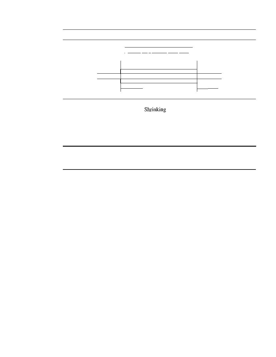
730
CHAPTER
23
PROCESS- TO-PROCESS DELNERY: UDp, TCP, AND SCTP
Figure 23.22
Sliding window
I
Window size
=
minimum (rwnd, cwnd)
p
g
Clos g
Shrinking
I • •• In-I
n
In+ll
...
1m-II m m+ll
...
I
Sliding window
in
o
enin
need not worry about them anymore.
the window means moving the right wall
to the left. This is strongly discouraged and not allowed in some implementations
because it means revoking the eligibility of some bytes for sending. This is a problem if
the sender has already sent these bytes. Note that the left wall cannot move to the left
because this would revoke some of the previously sent acknowledgments.
A sliding window is used to make transmission more efficient as weD as
to control the flow of data so that the destination does not become
overwhelmed with data. TCP sliding windows are byte-oriented.
The size of the window at one end is determined by the lesser of two values: receiver
window (rwnd) or congestion window (cwnd). The receiver window is the value adver-
tised by the opposite end in a segment containing acknowledgment.
It
is the number of
bytes the other end can accept before its buffer overflows and data are discarded. The
congestion window is a value determined by the network to avoid congestion. We will
discuss congestion later in the chapter.
Example 23.4
What is the value of the receiver window (rwnd) for host A if the receiver, host B, has a buffer
size of 5000 bytes and 1000 bytes of received and unprocessed data?
Solution
The value of rwnd
=
5000 - 1000
=
4000. Host B can receive only 4000 bytes of data before
overflowing its buffer. Host B advertises this value in its next segment to A.
Example 23.5
What is the size of the window for host A if the value of rwnd is 3000 bytes and the value of cwnd
is 3500 bytes?
Solution
The size of the window is the smaller of rwnd and cwnd, which is 3000 bytes.
Example
23.6
Figure 23.23 shows an unrealistic example of a sliding window. The sender has sent bytes up to
202. We assume that cwnd is 20 (in reality this value is thousands of bytes). The receiver has sent
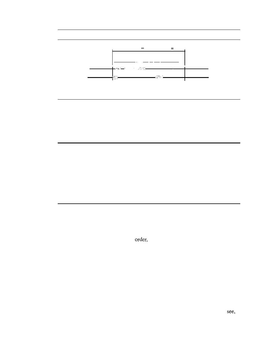
SECTION
23.3
TCP
731
Figure 23.23
Example 23.6
Window size
minimum (20, 9 )
9
Sent, not
acknowledged
I
Can be sent inunediately
1 •••
1199 2001201120212031204120520612071208 2091
•••
1
Sent and
acknowledged
•
Next byte to be sent
Can't be
sent until window
opens
an acknowledgment number of 200 with an
rwnd
of 9 bytes (in reality this value is thousands of
bytes). The size of the sender window is the minimum of
rwnd
and
cwnd,
or 9 bytes. Bytes 200 to
202 are sent, but not acknowledged. Bytes 203 to 208 can be sent without worrying about
acknowledgment. Bytes 209 and above cannot be sent.
Some points about TCP sliding windows:
o
The size of the window is the lesser of
rwnd
and
cwnd.
o
The source does not have to send a full window's worth of data.
o
The window can be opened or closed by the receiver, but should not be shrunk.
o
The destination can send an acknowledgment at any time as long as it does not result in
a shrinking window.
o
The receiver can temporarily shut down the window; the sender, however, can always
send a segment of 1 byte after the window is shut down.
Error Control
TCP is a reliable transport layer protocol. This means that an application program that
delivers a stream of data to TCP relies on TCP to deliver the entire stream to the appli-
cation program on the other end in
without error, and without any part lost or
duplicated.
TCP provides reliability using error control. Error control includes mechanisms for
detecting corrupted segments, lost segments, out-of-order segments, and duplicated
segments. Error control also includes a mechanism for correcting errors after they are
detected. Error detection and correction in TCP is achieved through the use of three
simple tools: checksum, acknowledgment, and time-out.
Checksum
Each segment includes a checksum field which is used to check for a corrupted segment.
If
the segment is corrupted, it is discarded by the destination TCP and is considered
as lost. TCP uses a 16-bit checksum that is mandatory in every segment. We will
in
Chapter 24, that the 16-bit checksum is considered inadequate for the new transport

732
CHAPTER
23
PROCESS-TO-PROCESS DELIVERY: UDp, TCp, AND SCTP
layer, SCTP. However, it cannot be changed for TCP because this would involve recon-
figuration of the entire header format.
Acknowledgment
TCP uses acknowledgments to confirm the receipt of data segments. Control segments
that carry no data but consume a sequence number are also acknowledged. ACK segments
are never acknowledged.
ACK segments do not consume sequence numbers and are not acknowledged.
Retransmission
The heart of the error control mechanism is the retransmission of segments. When a
segment is corrupted, lost, or delayed, it is retransmitted. In modern implementations, a
segment is retransmitted on two occasions: when a retransmission timer expires or
when the sender receives three duplicate ACKs.
In modern implementations, a retransmission occurs if the retransmission
timer expires or three duplicate ACK segments have arrived.
Note that no retransmission occurs for segments that do not consume sequence
numbers. In particular, there is no transmission for an ACK segment.
No retransmission timer is set for an ACK segment.
Retransmission After RTO
A recent implementation of TCP maintains one retrans-
mission time-out (RTO) timer for all outstanding (sent, but not acknowledged) seg-
ments. When the timer matures, the earliest outstanding segment is retransmitted even
though lack of a received ACK can be due to a delayed segment, a delayed ACK, or a lost
acknowledgment. Note that no time-out timer is set for a segment that carries only an
acknowledgment, which means that no such segment is resent. The value of RTO is
dynamic in TCP and is updated based on the round-trip time (RTT) of segments.
An
RTI is the time needed for a segment to reach a destination and for an acknowledgment
to be received.
It
uses a back-off strategy similar to one discussed in Chapter 12.
Retransmission After Three Duplicate ACK Segments
The previous rule about
retransmission of a segment is sufficient if the value of RTO is not very large. Sometimes,
however, one segment is lost and the receiver receives so many out-of-order segments
that they cannot be saved (limited buffer size). To alleviate this situation, most imple-
mentations today follow the three-duplicate-ACKs rule and retransmit the missing
segment immediately. This feature is referred to as fast retransmission, which we will
see in an example shortly.
Out-oj-Order Segments
When a segment is delayed, lost, or discarded, the segments following that segment arrive
out of order. Originally, TCP was designed to discard
all
out-of-order segments, resulting
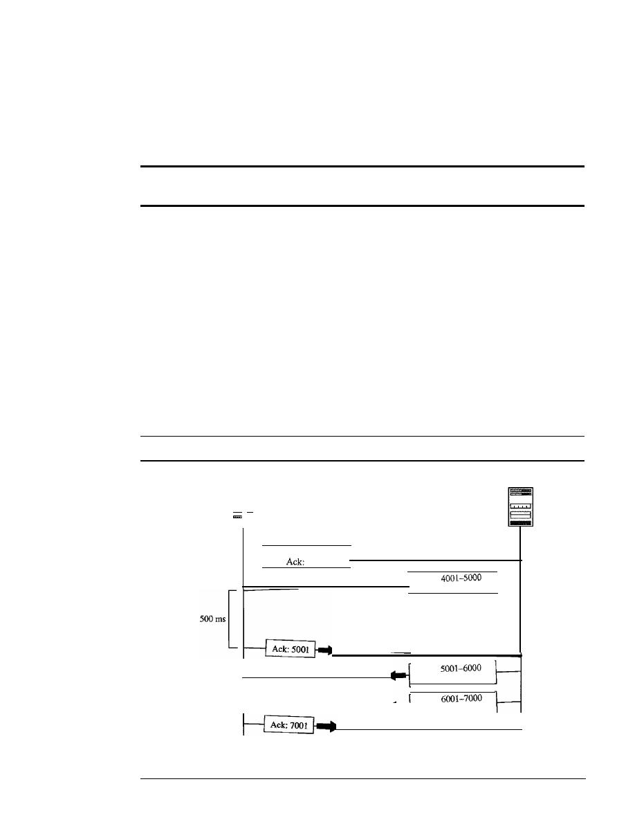
SECTION
23.3
TCP
733
in the retransmission of the missing segment and the following segments. Most imple-
mentations today do not discard the out-of-order segments. They store them temporarily
and flag them as out-of-order segments until the missing segment arrives. Note, however,
that the out-of-order segments are not delivered to the process. TCP guarantees that data
are delivered to the process in order.
Data may arrive out of order and be temporarily stored by the receiving TCP,
but
yep
guarantees that no out-of-order segment is delivered to the process.
Some Scenarios
In this section we give some examples of scenarios that occur during the operation of
TCP. In these scenarios, we show a segment by a rectangle.
If
the segment carries data,
we show the range of byte numbers and the value of the acknowledgment field.
If
it
carries only an acknowledgment, we show only the acknowledgment number in a
smaller box.
Normal Operation
The first scenario shows bidirectional data transfer between two
systems, as in Figure 23.24. The client TCP sends one segment; the server TCP sends
three. The figure shows which rule applies to each acknowledgment. There are data to
be sent, so the segment displays the next byte expected. When the client receives the
first segment from the server, it does not have any more data to send; it sends only an
Figure 23.24
Nonnaloperation
Server
Client
....
Seq:
1201-1400
4001
Time
Seq:
Ack:
1401
Seq:
Ack:
1401
Seq:
Ack: 1401
Time
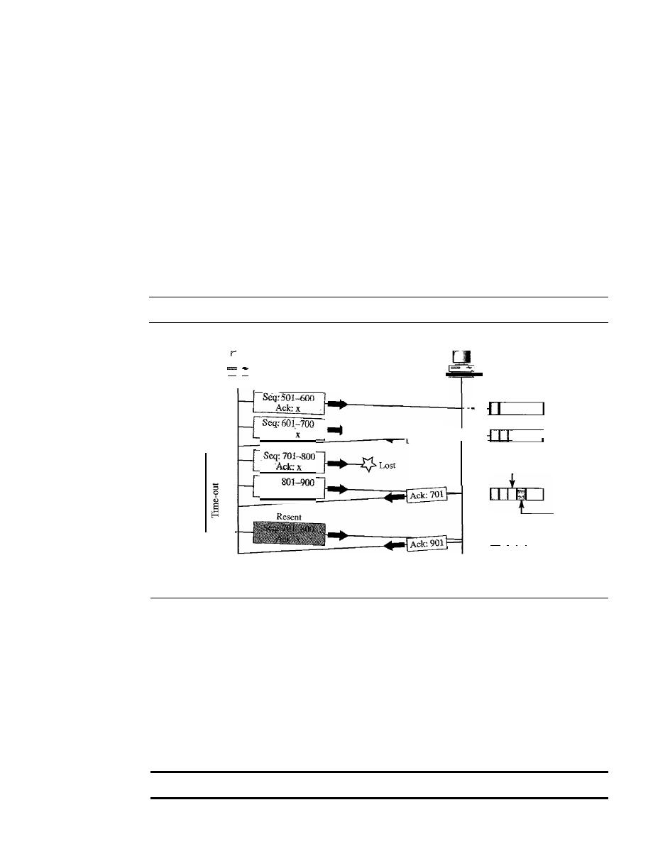
734
CHAPTER
23
PROCESS-TO-PROCESS DELIVERY: UDp, TCp, AND SCTP
ACK segment. However, the acknowledgment needs to be delayed for 500 ms to see if
any more segments arrive. When the timer matures, it triggers an acknowledgment.
This is so because the client has no knowledge if other segments are coming; it cannot
delay the acknowledgment forever. When the next segment arrives, another acknowl-
edgment timer is set. However, before it matures, the third segment arrives. The arrival
of the third segment triggers another acknowledgment.
Lost Segment
In this scenario, we show what happens when a segment is lost or cor-
rupted. A lost segment and a corrupted segment are treated the same way by the
receiver. A lost segment is discarded somewhere in the network; a corrupted segment is
discarded by the receiver itself. Both are considered lost. Figure 23.25 shows a situa-
tion in which a segment is lost and discarded by some router in the network, perhaps
due to congestion.
Figure 23.25
Lost segment
Receiver
buffer
Out of order
Gap
II I I I
Receiver
Seq:
Ack:x
--
Ack:
Ack: 701
----
Sender
RTO
Time
Time
We are assuming that data transfer is unidirectional: one site is sending, the other is
receiving. In our scenario, the sender sends segments 1 and 2, which are acknowledged
immediately by an ACK. Segment 3, however, is lost. The receiver receives segment 4,
which is out of order. The receiver stores the data in the segment in its buffer but leaves
a gap to indicate that there is no continuity in the data. The receiver immediately sends
an acknowledgment to the sender, displaying the next byte it expects. Note that the
receiver stores bytes 801 to 900, but never delivers these bytes to the application until
the gap is filled.
The receiver TCP delivers only ordered data to the process.
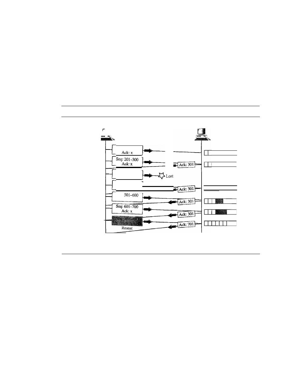
SECTION
23.3
TCP
735
We have shown the timer for the earliest outstanding segment. The timer for this
definitely runs out because the receiver never sends an acknowledgment for lost or out-
of-order segments. When the timer matures, the sending TCP resends segment 3, which
arrives this time and is acknowledged properly. Note that the value in the second and
third acknowledgments differs according to the corresponding rule.
Fast Retransmission
In
this scenario, we want to show the idea of fast retransmis-
sion. Our scenario is the same as the second except that the RTO has a higher value (see
Figure 23.26).
Figure 23.26
Fast retransmission
Sender
Seq: 101-200
Seq: 301-400
Ack:x
Seq:
401-500
Ack:x
Seq:
Ack:x
3ACKs--
Time
Receiver
Receiver
buffer
I I I I
All in
order
Time
When the receiver receives the fourth, fifth, and sixth segments, it triggers an
acknowledgment. The sender receives four acknowledgments with the same value (three
duplicates). Although the timer for segment 3 has not matured yet, the fast transmission
requires that segment 3, the segment that is expected by all these acknowledgments, be
resent immediately.
Note that only one segment is retransmitted although four segments are not
acknowledged. When the sender receives the retransmitted ACK, it knows that the four
segments are safe and sound because acknowledgment is cumulative.
Congestion Control
We discuss congestion control of TCP in Chapter 24.

736
CHAPTER
23
PROCESS-TO-PROCESS DELIVERY: UDp, TCp, AND SCTP
23.4
SCTP
Stream Control Transmission Protocol (SCTP) is a new reliable, message-oriented
transport layer protocol. SCTP, however, is mostly designed for Internet applications
that have recently been introduced. These new applications, such as IUA (ISDN over
IP), M2UA and M3UA (telephony signaling), H.248 (media gateway control), H.323
(IP telephony), and SIP (IP telephony), need a more sophisticated service than TCP can
provide. SCTP provides this enhanced performance and reliability. We briefly compare
UDP, TCP, and SCTP:
o
UDP is a message-oriented protocol. A process delivers a message to UDP, which
is encapsulated in a user datagram and sent over the network. UDP
conserves the
message boundaries;
each message is independent of any other message. This is a
desirable feature when we are dealing with applications such as IP telephony and
transmission of real-time data, as we will see later in the text. However, UDP is
unreliable; the sender cannot know the destiny of messages sent. A message can be
lost, duplicated, or received out of order. UDP also lacks some other features, such
as congestion control and flow control, needed for a friendly transport layer protocol.
o
TCP is a byte-oriented protocol.
It
receives a message or messages from a pro-
cess, stores them as a stream of bytes, and sends them in segments. There is no
preservation of the message boundaries. However, TCP is a reliable protocol.
The duplicate segments are detected, the lost segments are resent, and the bytes
are delivered to the end process in order. TCP also has congestion control and
flow control mechanisms.
o
SCTP combines the best features of UDP and TCP. SCTP is a reliable message-
oriented protocol. It preserves the message boundaries and at the same time detects
lost data, duplicate data, and out-of-order data.
It
also has congestion control and
flow control mechanisms. Later we will see that SCTP has other innovative features
unavailable in UDP and TCP.
SCTP is a message-oriented, reliable protocol that
combines the best features of UDP and TCP.
SCTP Services
Before we discuss the operation of SCTP, let us explain the services offered by SCTP to
the application layer processes.
Process-to-Process Communication
SCTP uses all well-known ports in the TCP space. Table 23.4 lists some extra port
numbers used by SCTP.
Multiple Streams
We learned in the previous section that TCP is a stream-oriented protocol. Each con-
nection between a TCP client and a TCP server involves one single stream. The problem
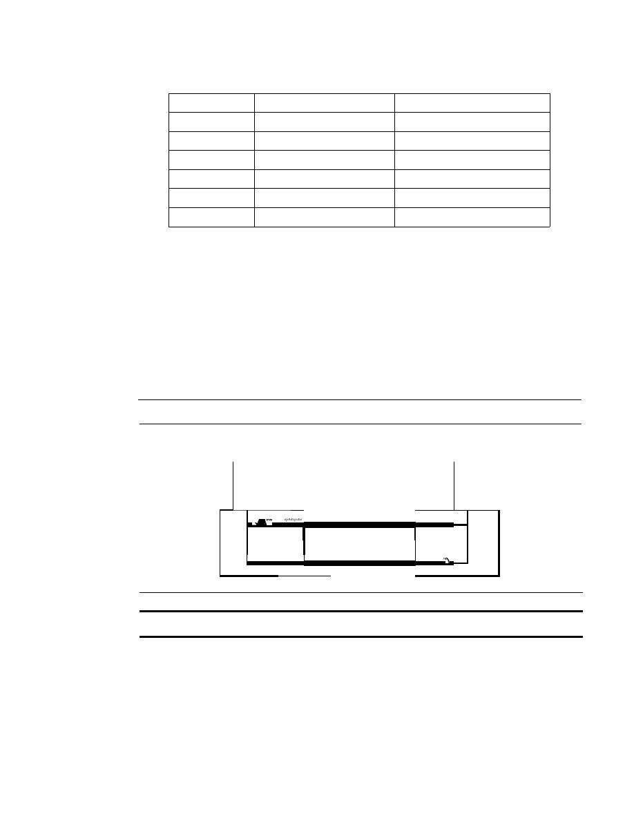
SECTION
23.4
SCTP
737
Table 23.4
Some SCTP applications
Protocol
Port Number
Description
IVA
9990
ISDN overIP
M2UA
2904
SS7 telephony signaling
M3UA
2905
SS7 telephony signaling
H.248
2945
Media gateway control
H.323
1718,1719, 1720, 11720
IP telephony
SIP
5060
IP telephony
with this approach is that a loss at any point in the stream blocks the delivery of the rest
of the data. This can be acceptable when we are transferring text; it is not when we are
sending real-time data such as audio or video. SCTP allows multistream service in
each connection, which is called association in SCTP terminology. If one of the streams
is blocked, the other streams can still deliver their data.The idea is similar to multiple
lanes on a highway. Each lane can be used for a different type of traffic. For example,
one lane can be used for regular traffic, another for car pools. If the traffic is blocked for
regular vehicles, car pool vehicles can still reach their destinations. Figure 23.27 shows
the idea of multiple-stream delivery.
Figure 23.27
Multiple-stream concept
Receiving
process
Sending
process
D
D
•
•
·
•
SCTP
•
SCTP
An association in SCTP can involve multiple streams.
Multihoming
A TCP connection involves one source and one destination IP address. This means that
even if the sender or receiver is a multihomed host (connected to more than one physi-
cal address with multiple IP addresses), only one of these IP addresses per end can be
utilized during the connection. An SCTP association, on the other hand, supports
multihoming service. The sending and receiving host can define multiple IP addresses
in each end for an association. In this fault-tolerant approach, when one path fails,
another interface can be used for data delivery without interruption. This fault-tolerant
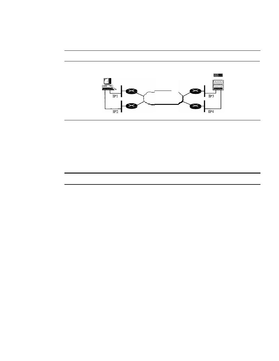
738
CHAPTER
23
PROCESS-TO-PROCESS DELIVERY: UDP, TCP, AND seTP
feature is very helpful when we are sending and receiving a real-time payload such as
Internet telephony. Figure 23.28 shows the idea of multihoming.
Figure 23.28
Multihoming concept
Client
Internet
Server
In Figure 23.28, the client is connected to two local networks with two IP addresses.
The server is also connected to two networks with two IP addresses. The client and the
server can make an association, using four different pairs of IP addresses. However, note
that in the current implementations of SCTP, only one pair of IF addresses can be chosen
for normal communication; the alternative is used if the main choice fails. In other
words, at present, SCTP does not allow load sharing between different paths.
SCTP association allows multiple IP addresses for each end.
Full-Duplex Communication
Like TCP, SCTP offers full-duplex service, in which data can flow in both directions at
the same time. Each SCTP then has a sending and receiving buffer, and packets are sent
in both directions.
Connection-Oriented Service
Like TCP, SCTP is a connection-oriented protocol. However, in SCTP, a connection is
called an association. When a process at site A wants to send and receive data from
another process at site B, the following occurs:
1. The two SCTPs establish an association between each other.
2. Data are exchanged in both directions.
3. The association is terminated.
Reliable Service
SCTP, like TCP, is a reliable transport protocol. It uses an acknowledgment mechanism
to check the safe and sound arrival of data. We will discuss this feature further in the
section on error control.
SCTP Features
Let us first discuss the general features of SCTP and then compare them with those ofTCP.

SECTION
23.4
SCTP
739
Transmission Sequence Number
The unit of data in TCP is a byte. Data transfer in TCP is controlled by numbering bytes
by using a sequence number. On the other hand, the unit of data in SCTP is a DATA chunk
which mayor may not have a one-to-one relationship with the message coming from the
process because of fragmentation (discussed later), Data transfer in SCTP is controlled
by numbering the data chunks. SCTP uses a
transmission sequence number
(TSN) to
number the data chunks. In other words, the TSN in SCTP plays the analogous role to
the sequence number in TCP. TSNs are 32 bits long and randomly initialized between 0
and 2
32
-
1. Each data chunk must carry the corresponding TSN in its header.
In
a data chunk is numbered using a TSN.
Stream Identifier
In TCP, there is only one stream in each connection. In SCTP, there may be several
streams in each association. Each stream in SCTP needs to be identified by using a
stream identifier (SI).
Each data chunk must carry the SI in its header so that when it
arrives at the destination, it can be properly placed in its stream. The 51 is a 16-bit number
starting from
O.
To distinguish between different streams, SCTP uses an SI.
Stream Sequence Number
When a data chunk arrives at the destination SCTP,
it
is delivered to the appropriate
stream and in the proper order. This means that, in addition to an SI, SCTP defines each
data chunk in each stream with a
stream sequence number
(SSN).
To distinguish between different data chunks belonging
to the same stream, SCTP uses SSNs.
Packets
In TCP, a segment carries data and control information. Data are carried as a collection
of bytes; control information is defined by six control flags in the header. The design of
SCTP is totally different: data are carried as data chunks, control information is carried
as control chunks. Several control chunks and data chunks can be packed together in a
packet. A packet in SCTP plays the same role as a segment in TCP. Figure 23.29 compares
a segment in TCP and a packet in SCTP. Let us briefly list the differences between an
SCTP packet and a TCP segment:
TCP has segments; SCTP has packets.
1. The control information in TCP is part of the header; the control information in
SCTP is included in the control chunks. There are several types of control chunks;
each is used for a different purpose.
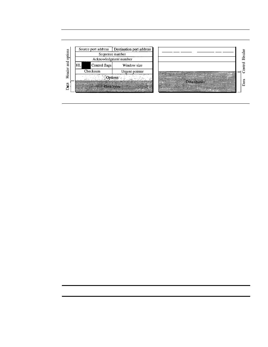
740
CHAPTER
23
PROCESS-TO-PROCESS DELIVERY: UDp, TCp, AND SCTP
Figure 23.29
Comparison between a TCP segment and an SCTP packet
Checksum
]
Control chunks
Source port address
Destination port address
]
Verification tag
A segment in TCP
A packet in SCTP
2. The data in a TCP segment treated as one entity; an SCTP packet can carry several
data chunks; each can belong to a different stream.
3. The options section, which can be part of a TCP segment, does not exist in an
SCTP packet. Options in SCTP are handled by defining new chunk types.
4. The mandatory part of the TCP header is 20 bytes, while the general header in
SCTP is only 12 bytes. The SCTP header is shorter due to the following:
a. An SCTP sequence number (TSN) belongs to each data chunk and hence is
located in the chunk's header.
b. The acknowledgment number and window size are part of each control chunk.
c. There is no need for a header length field (shown as HL in the TCP segment)
because there are no options to make the length of the header variable; the
SCTP header length is fixed (12 bytes).
d. There is no need for an urgent pointer in SCTP.
5. The checksum in TCP is 16 bits; in SCTP, it is 32 bits.
6. The verification tag in SCTP is an association identifier, which does not exist in
TCP. In TCP, the combination of IP and port addresses defines a connection; in
SCTP we may have multihorning using different IP addresses. A unique verification
tag is needed to define each association.
7. TCP includes one sequence number in the header, which defines the number of the
first byte in the data section. An SCTP packet can include several different data
chunks. TSNs, SIs, and SSNs define each data chunk.
8. Some segments in TCP that carry control information (such as SYN and FIN) need
to consume one sequence number; control chunks in SCTP never use a TSN, SI, or
SSN. These three identifiers belong only to data chunks, not to the whole packet.
In SCTP, control information and data information are carried in separate chunks.
In SCTP, we have data chunks, streams, and packets.
An
association may send many
packets, a packet may contain several chunks, and chunks may belong to different
streams. To make the definitions of these terms clear, let us suppose that process A
needs to send 11 messages to process B in three streams. The first four messages are in
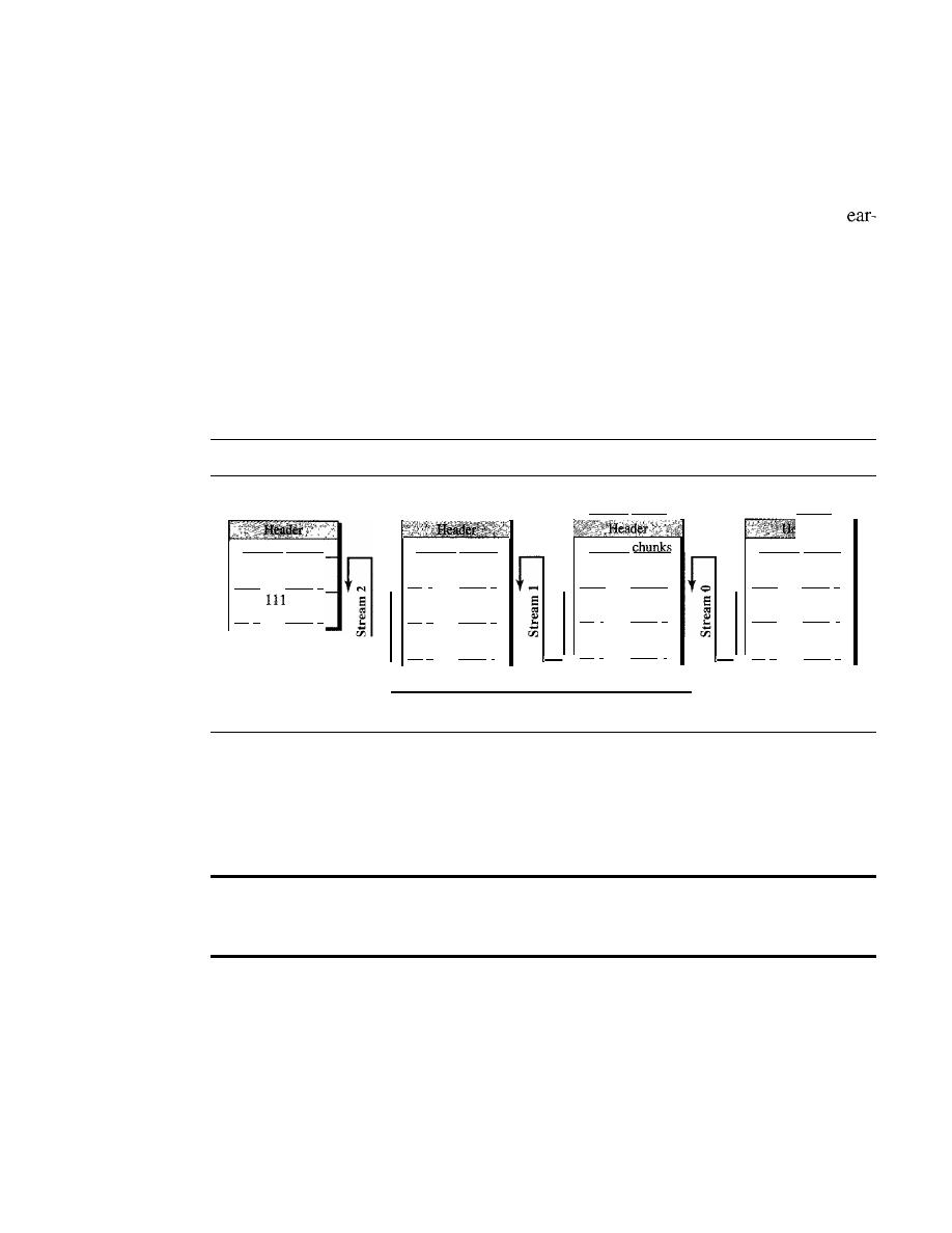
SECTION
23.4
SCTP
741
the first stream, the second three messages are in the second stream, and the last four
messages are in the third stream.
Although a message, if long, can be carried by several data chunks, we assume that
each message fits into one data chunk. Therefore, we have 11 data chunks in three streams.
The application process delivers 11 messages to SCTP, where each message is
marked for the appropriate stream. Although the process could deliver one message from
the first stream and then another from the second, we assume that it delivers all messages
belonging to the first stream first,
all
messages belonging to the second stream next, and
finally, all messages belonging to the last stream.
We also assume that the network allows only three data chunks per packet, which
means that we need. four packets as shown in Figure 23.30. Data chunks in stream 0 are
carried
in
the first packet and part of the second packet; those in stream 1 are carried
in
the second and third packets; those in stream 2 are carried in the third and fourth packets.
Figure 23.30
Packet, data chunks, and streams
First packet
Control chunks
TSN: 101
SI:O
SSN:
0
TSN:
102
SI:O
SSN: 1
TSN: 103
SI: 0
SSN: 2
Second packet
Control
T5N: 104
SI:O
SSN:3
TSN:
105
SI:
1
SSN:
0
TSN:
106
SI:
1
SSN:
1
Third packet
Control chunks
TSN: 107
SI:
1
SSN:
2
::rSN:
108
SI: 2
SSN:
0
TSN:
109
SI:
2
SSN: 1
Fourth packet
Control chunks
TSN: llO
SI:2
SSN: 2
TSN:
51: 2
SSN:
3
Flow of packets from sender to receiver
Note that each data chunk needs three identifiers: TSN, SI, and SSN. TSN is a
cumulative number and is used, as we will see later, for flow control and error control.
SI defines the stream to which the chunk belongs. SSN defines the chunk's order in a
particular stream.
In
our example, SSN starts from 0 for each stream.
Data chunks are identified by three items: TSN, SI, and SSN.
TSN is a cumulative number identifying the association;
SI defines the stream; SSN defines the chunk in a stream.
Acknowledgment Number
TCP acknowledgment numbers are byte-oriented and refer to the sequence numbers.
SCTP acknowledgment numbers are chunk-oriented. They refer to the TSN. A second
difference between TCP and SCTP acknowledgments is the control information. Recall
that this information is part of the segment header in TCP. To acknowledge segments
that carry only control information, TCP uses a sequence number and acknowledgment
number (for example, a SYN segment needs to be acknowledged by an ACK segment).
In SCTP, however, the control information is carried by control chunks, which do not
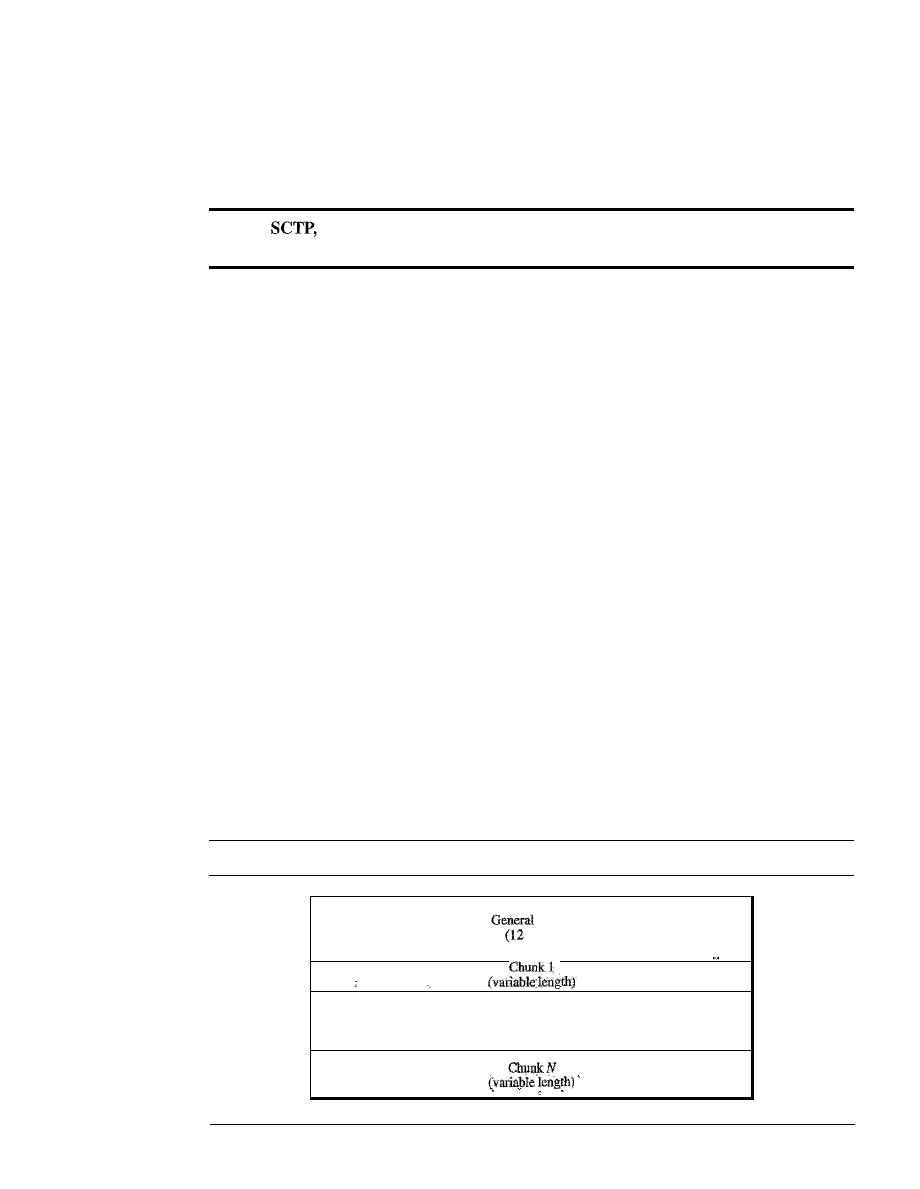
742
CHAPTER
23
PROCESS-TO-PROCESS DELIVERY: UDp, TCp, AND SCTP
need a TSN. These control chunks are acknowledged by another control chunk of the
appropriate type (some need no acknowledgment). For example, an INIT control chunk
is acknowledged by an INIT ACK chunk. There is no need for a sequence number or an
acknowledgment number.
In
acknowledgment numbers are used to acknowledge only data chunks;
control chunks are acknowledged
by
other control chunks
if
necessary.
Flow Control
Like TCP, SCTP implements flow control to avoid overwhelming the receiver. We will
discuss SCTP flow control later in the chapter.
Error Control
Like TCP, SCTP implements error control to provide reliability. TSN numbers and
acknowledgment numbers are used for error control. We will discuss error control later
in the chapter.
Congestion Control
Like TCP, SCTP implements congestion control to determine how many data chunks
can be injected into the network. We will discuss congestion control in Chapter 24.
Packet Format
In this section, we show the format of a packet and different types of chunks. Most of
the information presented in this section will become clear later; this section can be
skipped in the first reading or used only as a reference. An SCTP packet has a mandatory
general header and a set of blocks called chunks. There are two types of chunks: control
chunks and data chunks. A control chunk controls and maintains the association; a data
chunk carries user data. In a packet, the control chunks corne before the data chunks.
Figure 23.31 shows the general format of an SCTP packet.
Figure 23.31
SCTP packet format
header
bytes)
···
SECTION
23.4
SCTP
743
In an SCTP packet, control chunks come before data chunks.
General Header
The
general header
(packet header) defines the endpoints of each association to which
the packet belongs, guarantees that the packet belongs to a particular association, and
preserves the integrity of the contents of the packet including the header itself. The fonnat
of the general header is shown in Figure 23.32.
Figure 23.32
General header
Source port address
I
Destination port address
16 bits
16 bits
Verification tag
32 bits
Checksum
32 bits
There are four fields in the general header:
o
Source port address.
This is a 16-bit field that defines the port number of the pro-
cess sending the packet.
o
Destination port address.
This is a 16-bit field that defines the port number of the
process receiving the packet.
o
Verification tag.
This is a number that matches a packet to an association. This
prevents a packet from a previous association from being mistaken as a packet in
this association. It serves as an identifier for the association; it is repeated in every
packet during the association. There is a separate verification used for each direction
in the association.
o
Checksum.
This 32-bit field contains a CRC-32 checksum. Note that the size of
the checksum is increased from 16 (in UDP, TCP, and IP) to 32 bits to allow the
use of the CRC-32 checksum.
Chunks
Control infonnation or user data are carried in chunks. The detailed fonnat of each chunk
is beyond the scope of this book. See [For06] for details. The first three fields are com-
mon to all chunks; the information field depends on the type of chunk. The important
point to remember is that SCTP requires the information section to be a multiple of
4 bytes; if not, padding bytes (eight as) are added at the end of the section. See Table 23.5
for a list of chunks and their descriptions.
An SCTP Association
SCTP, like TCP, is a connection-oriented protocol. However, a connection in SCTP is
called an
association
to emphasize multihoming.

744
CHAPTER
23
PROCESS-TO-PROCESS DEliVERY: UDp, TCp' AND SCTP
Table 23.5
Chunks
Type
Chunk
Description
0
DATA
User data
1
INIT
Sets up an association
2
INITACK
Acknowledges INIT chunk
3
SACK
Selective acknowledgment
4
HEARTBEAT
Probes the peer for liveliness
5
HEARTBEAT ACK
Acknowledges HEARTBEAT chunk
6
ABORT
Aborts an association
7
SHUTDOWN
Terminates an association
8
SHUTDOWN ACK
Acknowledges SHUTDOWN chunk
9
ERROR
Reports errors without shutting down
10
COOKIE ECHO
Third packet in association establishment
11
COOKIEACK
Acknowledges COOKIE ECHO chunk
14
SHUTDOWN COMPLETE
Third packet in association termination
192
FORWARDTSN
For adjusting cumulative TSN
A connection in SCTP is called an association.
Association Establishment
Association establishment in SCTP requires a four-way handshake. In this proce-
dure, a process, normally a client, wants to establish an association with another process,
normally a server, using SCTP as the transport layer protocol. Similar to TCP, the
SCTP server needs to be prepared to receive any association (passive open). Associa-
tion establishment, however, is initiated by the client (active open). SCTP association
establishment is shown in Figure 23.33. The steps, in a normal situation, are as follows:
1. The client sends the first packet, which contains an INIT chunk.
2. The server sends the second packet, which contains an INIT ACK chunk.
3. The client sends the third packet, which includes a COOKIE ECHO chunk. This
is a very simple chunk that echoes, without change, the cookie sent by the server.
SCTP allows the inclusion of data chunks in this packet.
4. The server sends the fourth packet, which includes the COOKIE ACK chunk that
acknowledges the receipt of the COOKIE ECHO chunk. SCTP allows the inclusion
of data chunks with this packet.
No other chunk is allowed in a packet carrying an INIT or INIT ACK chunk.
A COOKIE ECHO or a COOKIE ACK chunk can carry
data
chunks.
Cookie
We discussed a SYN flooding attack in the previous section. With TCP, a
malicious attacker can flood a TCP server with a huge number of phony SYN segments
using different forged IP addresses. Each time the server receives a SYN segment, it
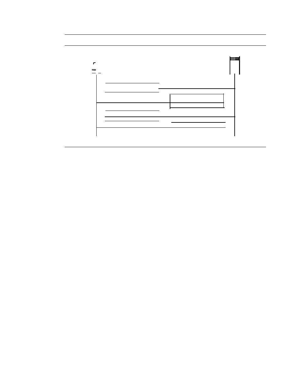
SECTION
23.4
SCTP
745
Figure 23.33
Four-way handshaking
Client
-
INIT
COOKIE ECHO
Cookie
Time
INITACK
Cookie
COOKIEACK
Server
Time
sets up a state table and allocates other resources while waiting for the next segment to
arrive. After a while, however, the server may collapse due to the exhaustion of resources.
The designers of SCTP have a strategy to prevent this type of attack. The strategy
is to postpone the allocation of resources until the reception of the third packet, when
the IP address of the sender is verified. The information received in the first packet must
somehow be saved until the third packet arrives. But if the server saved the information,
that would require the allocation of resources (memory); this is the dilemma. The solution
is to pack the information and send it back to the client. This is called generating a
cookie. The cookie is sent with the second packet to the address received in the first
packet. There are two potential situations.
1.
If
the sender of the first packet is an attacker, the server never receives the third
packet; the cookie is lost and no resources are allocated. The only effort for the
server is "baking" the cookie.
2. If the sender of the first packet is an honest client that needs to make a connection,
it receives the second packet, with the cookie.
It
sends a packet (third in the series)
with the cookie, with no changes. The server receives the third packet and knows
that it has come from an honest client because the cookie that the sender has sent is
there. The server can now allocate resources.
The above strategy works if no entity can "eat" a cookie "baked" by the server. To guar-
antee this, the server creates a digest (see Chapter 30) from the information, using its
own secret key. The information and the digest together make the cookie, which is sent
to the client in the second packet. When the cookie is returned in the third packet, the
server calculates the digest from the information.
If
the digest matches the one that is
sent, the cookie has not been changed by any other entity.
Data Transfer
The whole purpose of an association is to transfer data between two ends. After the
association is established, bidirectional data transfer can take place. The client and the
server can both send data. Like TCP, SCTP supports piggybacking.
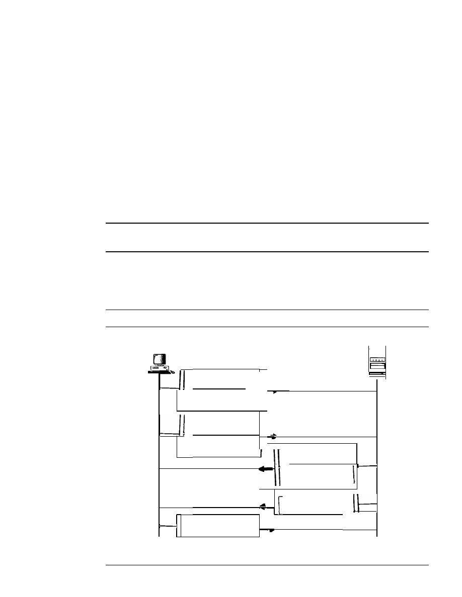
746
CHAPTER
23
PROCESS-TO-PROCESS DELNERY: UDp, TCp, AND SCTP
There is a major difference, however, between data transfer in TCP and SCTP. TCP
receives messages from a process as a stream of bytes without recognizing any boundary
between them. The process may insert some boundaries for its peer use, but TCP treats
that mark as part of the text. In other words, TCP takes each message and appends it to
its buffer. A segment can carry parts of two different messages. The only ordering sys-
tem imposed by TCP is the byte numbers.
SCTP, on the other hand, recognizes and maintains boundaries. Each message com-
ing from the process is treated as one unit and inserted into a DATA chunk unless it is
fragmented (discussed later). In this sense, SCTP is like UDP, with one big advantage:
data chunks are related to each other.
A message received from a process becomes a DATA chunk, or chunks if frag-
mented, by adding a DATA chunk header to the message. Each DATA chunk formed by
a message or a fragment of a message has one TSN. We need to remember that only
DATA chunks use TSNs and only DATA chunks are acknowledged by SACK chunks.
In
SCTP, only DATA chunks consume TSNs;
DATA chunks are the only chunks that are acknowledged.
Let us show a simple scenario in Figure 23.34. In this figure a client sends four
DATA chunks and receives two DATA chunks from the server. Later, we will discuss
Figure 23.34
Simple data transfer
Server
Client
i
TSN: 7105
I
DATA chunk
I
......
TSN:
7106
DATA chunk
TSN: 7107
1
DATA chunk
[
I
TSN: 7108
DATA chunk
\
cumTSN:
7108
SACK chunk
TSN:
121
DATA chunk
TSN:
122
DATA chunk
cumTSN:
122
I
.....
SACK chunk
Time
Time

SECTION
23.4
SCTP
747
the use of flow and error control in SCTP. For the moment, we assume that everything
goes well in this scenario.
1.
The client sends the first packet carrying two DATA chunks with TSNs 7105 and
7106.
2. The client sends the second packet carrying two DATA chunks with TSNs 7107
and 7108.
3. The third packet is from the server. It contains the SACK chunk needed to
acknowledge the receipt of DATA chunks from the client. Contrary to TCP,
SCTP acknowledges the last in-order TSN received, not the next expected. The
third packet also includes the first DATA chunk from the server with TSN 121.
4. After a while, the server sends another packet carrying the last DATA chunk with
TSN 122, but it does not include a SACK chunk in the packet because the last
DATA chunk received from the client was already acknowledged.
5. Finally, the client sends a packet that contains a SACK chunk acknowledging the
receipt of the last two DATA chunks from the server.
The acknowledgment in SCTP defines the cumulative TSN,
the TSN of the last data chunk received in order.
Multihoming Data Transfer
We discussed the multihoming capability of SCTP, a
feature that distinguishes SCTP from UDP and TCP. Multihoming allows both ends to
define multiple IP addresses for communication. However, only one of these addresses
can be defined as the primary address; the rest are alternative addresses. The primary
address is defined during association establishment. The interesting point is that the pri-
mary address of an end is determined by the other end. In other words, a source defines
the primary address for a destination.
Multistream Delivery
One interesting feature of SCTP is the distinction between
data transfer and data delivery. SCTP uses TSN numbers
to
handle data transfer, move-
ment of data chunks between the source and destination. The delivery of the data chunks
is controlled by SIs and SSNs. SCTP can support multiple streams, which means that
the sender process can define different streams and a message can belong to one of
these streams. Each stream is assigned a stream identifier (SI) which uniquely defines
that stream.
Fragmentation
Another issue in data transfer is fragmentation. Although SCTP
shares this term with IP, fragmentation in IP and in SCTP belongs to different levels:
the former at the network layer, the latter at the transport layer.
SCTP preserves the boundaries of the message from process to process when
creating a DATA chunk from a message if the size of the message (when encapsu-
lated in an IP datagram) does not exceed the MTU of the path. The size of an IP
datagram carrying a message can be determined by adding the size of the message, in
bytes, to the four overheads: data chunk header, necessary SACK chunks, SCTP gen-
eral header, and IP header.
If
the total size exceeds the MTU, the message needs to be
fragmented.
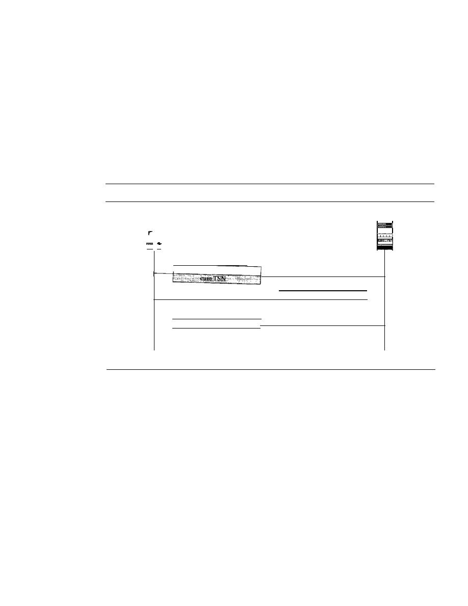
748
CHAPTER
23
PROCESS-TO-PROCESS DELIVERY: UDp, TCp, AND SCTP
Association Termination
In SCTP, like TCP, either of the two parties involved in exchanging data (client or
server) can close the connection. However, unlike TCP, SCTP does not allow a half-
close situation.
If
one end closes the association, the other end must stop sending new
data.
If
any data are left over in the queue of the recipient of the termination request,
they are sent and the association is closed. Association
termination uses three packets,
as shown in Figure 23.35. Note that although the figure shows the case in which termi-
nation is initiated by the client, it can also be initiated by the server. Note that there can
be several scenarios of association termination. We leave this discussion to the references
mentioned at the end of the chapter.
Figure 23.35
Association termination
Client
SHUTDOWN
Active
close
SHUTDOWN
COMPLETE
Time
Flow Control
SHUTDOWN ACK
Server
Passive
close
Time
Flow control in SCTP is similar to that in TCP. In TCP, we need to deal with only one
unit of data, the byte. In SCTP, we need to handle two units of data, the byte and the
chunk. The values of rwnd and cwnd are expressed in bytes; the values of TSN and
acknowledgments are expressed in chunks. To show the concept, we make some unre-
alistic assumptions. We assume that there is never congestion in the network and that
the network is error-free.
In
other words, we assume that cwnd is infinite and no packet is
lost or delayed or arrives out of order. We also assume that data transfer is unidirectional.
We correct our unrealistic assumptions in later sections. Current SCTP implementa-
tions still use a byte-oriented window for flow control. We, however, show the buffer in
terms of chunks to make the concept easier to understand.
Receiver Site
The receiver has one buffer (queue) and three variables. The queue holds the received
data chunks that have not yet been read by the process. The first variable holds the last
TSN received,
cumTSN. The second variable holds the available buffer size, winsize.
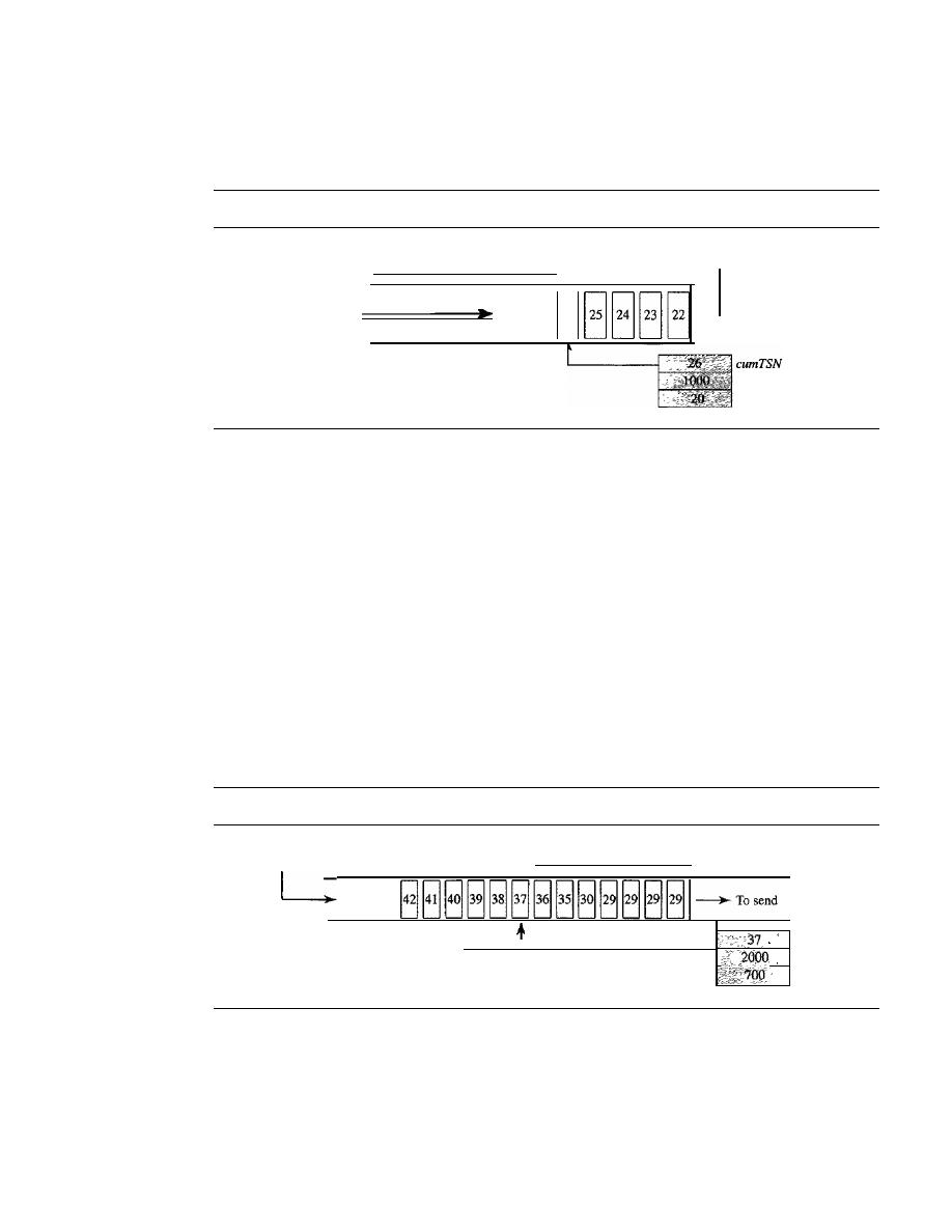
SECTION
23.4
SCTP
749
The third variable holds the last accumulative acknowledgment,
lastACK. Figure 23.36
shows the queue and variables at the receiver site.
Figure 23.36
Flow control, receiver site
winSize
Received
To process
26
Receiving queue
winSize
lastACK
1.
When the site receives a data chunk, it stores it at the end of the buffer (queue) and
subtracts the size of the chunk from winSize. The TSN number of the chunk is
stored in the cumTSN variable.
2. When the process reads a chunk, it removes it from the queue and adds the size of
the removed chunk to winSize (recycling).
3. When the receiver decides to send a SACK, it checks the value of
lastAck; if it is
less than cumTSN, it sends a SACK with a cumulative TSN number equal to the
cumTSN.
It also includes the value of winSize as the advertised window size.
Sender Site
The sender has one buffer (queue) and three variables: curTSN, rwnd, and inTransit, as
shown in Figure 23.37. We assume each chunk is 100 bytes long.
Figure 23.37
Flow control, sender site
curTSN
rwnd
inTransit
Outstanding chunks
Sending queue
From process
The buffer holds the chunks produced by the process that either have been sent or are
ready to be sent. The first variable, curTSN, refers to the next chunk to be sent. All chunks
in the queue with a TSN less than this value have been sent, but not acknowledged; they
are outstanding. The second variable, rwnd, holds the last value advertised by the receiver
(in bytes). The third variable, inTransit, holds the number of bytes in transit, bytes sent
but not yet acknowledged. The following is the procedure used by the sender.
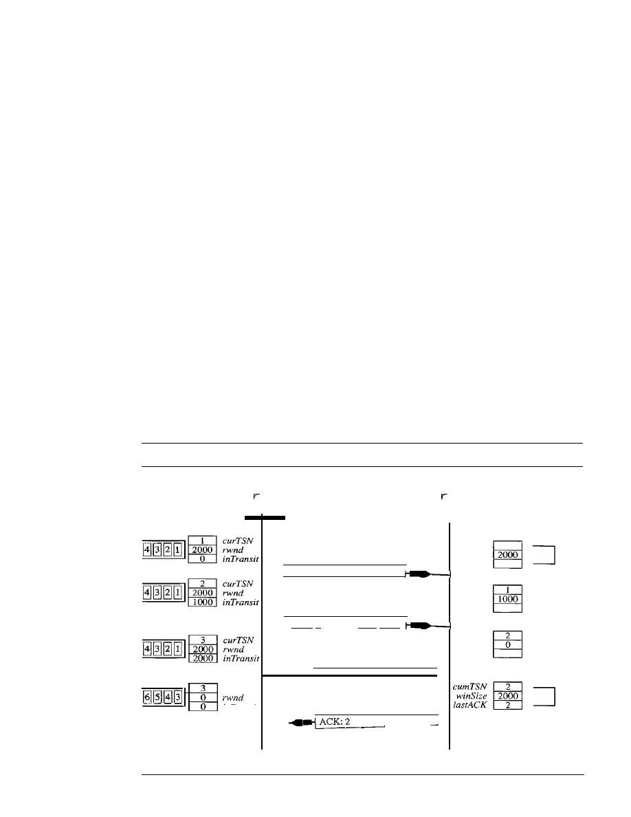
750
CHAPTER
23
PROCESS-TO-PROCESS DELIVERY: UDp, TCp, AND SCTP
1. A chunk pointed
to
by
curTSN
can be sent if the size of the data is less than or
equal to the quantity
rwnd - inTransit.
After sending the chunk, the value of
curTSN
is incremented by 1 and now points to the next chunk to be sent. The value of
inTransit
is incremented by the size of the data in the transmitted chunk.
2. When a SACK is received, the chunks with a TSN less than or equal to the cumula-
tive TSN in the SACK are removed from the queue and discarded. The sender does
not have to worry about them any more. The value of
inTransit
is reduced by the
total size of the discarded chunks. The value of
rwnd
is updated with the value of
the advertised window in the SACK.
A Scenario
Let us give a simple scenario as shown in Figure 23.38. At the start the value of
rwnd
at
the sender site and the value of
winSize
at the receiver site are 2000 (advertised during
association establishment). Originally, there are four messages in the sender queue. The
sender sends one data chunk and adds the number of bytes (1000) to the
inTransit
vari-
able. After awhile, the sender checks the difference between the
rwnd
and
inTransit,
which is 1000 bytes, so it can send another data chunk. Now the difference between the
two variables is 0 and no more data chunks can be sent. After awhile, a SACK arrives
that acknowledges data chunks 1 and 2. The two chunks are removed from the queue.
The value of
inTransit
is now
O. The SACK, however, advertised a receiver window of
value 0, which makes the sender.update
rwnd
to
O. Now the sender is blocked; it cannot
send any data chunks (with one exception explained later).
Figure 23.38
Flow control scenario
Sender
DATA
TSN: 1
Receiver
cumTSN
winSize
2000
lastACK
1000 bytes
DATA
cumTSN
winSize
1000
lastACK
curTSN
0
0
znTranslt
:ess writes
i
and 6
TSN: 2
1000 bytes
SACK
ACK: 2
rwnd:
°
SACK
l - - -
rw
_ n_d_:2_0_0_0
..
cumTSN
winSize
0
[astACK
winSize
2000
[astACK
2
Process reads
1
and 2
Time
Time
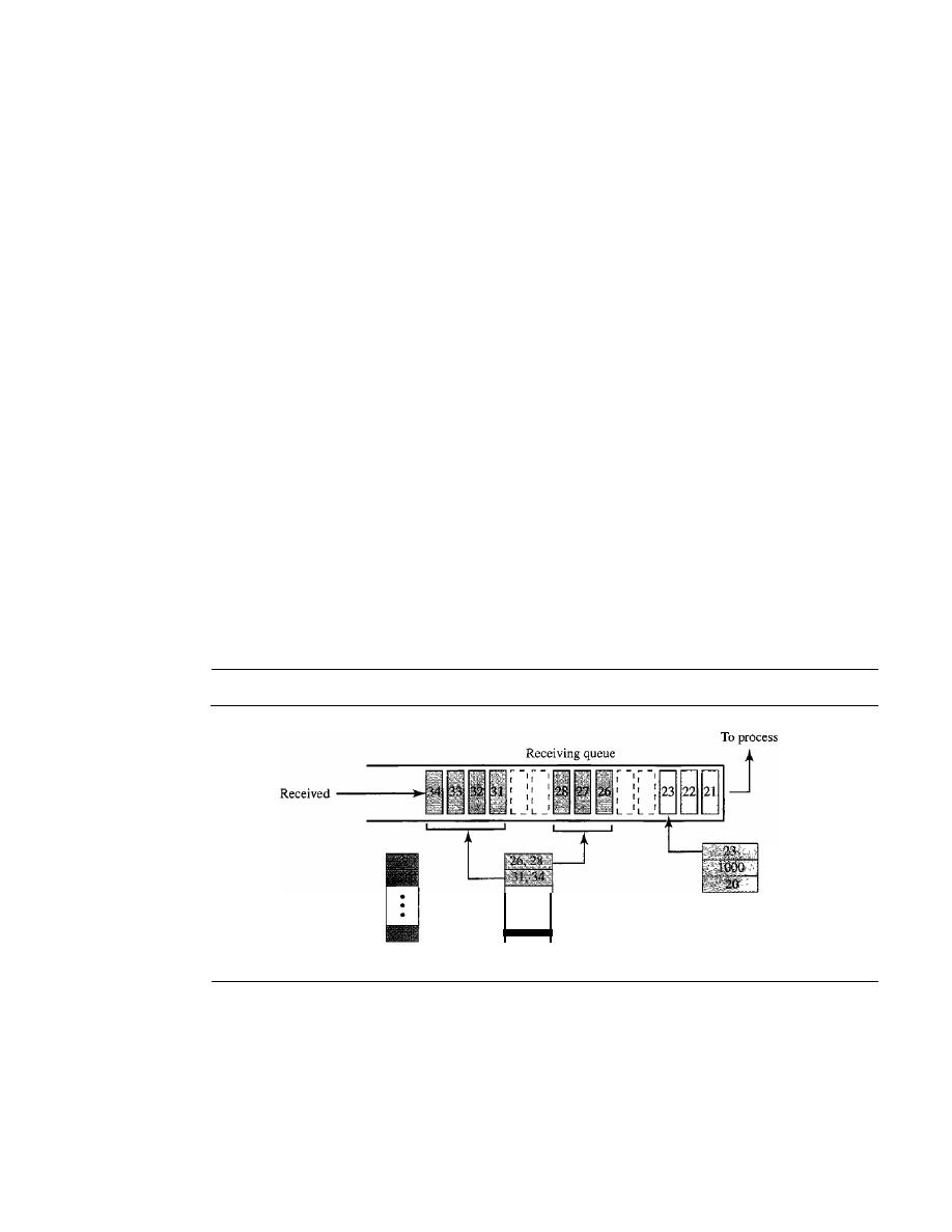
SECTION
23.4
SCTP
751
At the receiver site, the queue is empty at the beginning. After the first data chunk
is received, there is one message in the queue and the value of
cumTSN
is 1. The value
of
winSize
is reduced to 1000 because the first message occupies 1000 bytes. After the
second data chunk is received, the value of window size is
a
and
cumTSN
is 2. Now, as
we will see, the receiver is required to send a SACK with cumulative TSN of 2. After
the first SACK was sent, the process reads the two messages, which means that there is
now room in the queue; the receiver advertises the situation with a SACK to allow the
sender to send more data chunks. The remaining events are not shown in the figure.
Error Control
SCTP, like TCP, is a reliable transport layer protocol.
It
uses a SACK chunk to report
the state of the receiver buffer to the sender. Each implementation uses a different set of
entities and timers for the receiver and sender sites. We use a very simple design to convey
the concept to the reader.
Receiver Site
In
our design, the receiver stores all chunks that have arrived in its queue including the
out-of-order ones. However, it leaves spaces for any missing chunks.
It
discards dupli-
cate messages, but keeps track of them for reports to the sender. Figure 23.39 shows a
typical design for the receiver site and the state of the receiving queue at a particular
point in time.
Figure 23.39
Error control, receiver site
Duplicate
·
··
OutOfOrder
cumTSN
winSize
lastACK
The last acknowledgment sent was for data chunk 20. The available window size is
1000 bytes. Chunks 21 to 23 have been received in order. The first out-of-order block
contains chunks 26 to 28. The second out-of-order block contains chunks 31 to 34. A
variable holds the value of
cumTSN.
An array of variables keeps track of the beginning
and the end of each block that is out of order. An array of variables holds the duplicate
chunks received. Note that there is no need for storing duplicate chunks in the queue;
they will be discarded. The figure also shows the SACK chunk that will be sent to
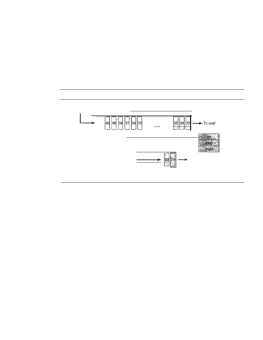
752
CHAPTER
23
PROCESS-TO-PROCESS DELNERY: UDp, TCp, AND SCTP
report the state of the receiver to the sender. The TSN numbers for out-of-order chunks
are relative (offsets) to the cumulative TSN.
Sender Site
At the sender site, our design demands two buffers (queues): a sending queue and a
retransmission queue. We also use the three variables
rwnd, inTransit,
and
curTSN
as
described in the previous section. Figure 23.40 shows a typical design.
Figure 23.40
Error control, sender site
From process
Outstanding chunks
...
inTransit
curTSN
rwnd
Retransmission
queue
Add when timer
expires or three
To send
SACKs are received.
-----====
Sending queue
The sending queue holds chunks 23 to 40. The chunks 23 to 36 have already been
sent, but not acknowledged; they are outstanding chunks. The
curTSN
points to the
next chunk to be sent (37). We assume that each chunk is 100 bytes, which means that
1400 bytes of data (chunks 23 to 36) is in transit. The sender at this moment has a
retransmission queue. When a packet is sent, a retransmission timer starts for that
packet (all data chunks in that packet). Some implementations use one single timer for
the entire association, but we continue with our tradition of one timer for each packet for
simplification. When the retransmission timer for a packet expires, or four duplicate
SACKs arrive that declare a packet as missing (fast retransmission was discussed in
Chapter 12), the chunks in that packet are moved to the retransmission queue to be
resent. These chunks are considered lost, rather than outstanding. The chunks in the
retransmission queue have priority. In other words, the next time the sender sends a
chunk, it would be chunk 21 from the retransmission queue.
Sending Data Chunks
An end can send a data packet whenever there are data chunks in the sending queue
with a TSN greater than or equal to
curTSN
or if there are data chunks in the retransmis-
sion queue. The retransmission queue has priority. However, the total size of the data
chunk or chunks included in the packet must not exceed
rwnd - inTrans it,
and the total
size of the frame must not exceed the MTU size as we discussed in previous sections.

SECTION
23.5
RECOMMENDED READING
753
Retransmission
To control a lost or discarded chunk, SCTP, like TCP, employs two
strategies: using retransmission timers and receiving four SACKs with the same missing
chunks.
Generating SACK Chunks
Another issue in error control is the generation of SACK chunks. The rules for generating
SCTP SACK chunks are similar to the rules used for acknowledgment with the TCP
ACK flag.
Congestion Control
SCTP, like TCP, is a transport layer protocol with packets subject to congestion in the net-
work. The SCTP designers have used the same strategies we will describe for congestion
control in Chapter 24 for TCP. SCTP has slow start (exponential increase), congestion
avoidance (additive increase), and congestion detection (multiplicative decrease) phases.
Like TCP, SCTP also uses fast retransmission and fast recovery.
23.5
RECOMMENDED READING
For more details about subjects discussed in this chapter, we recommend the following
books and sites. The items in brackets [...] refer to the reference list at the end of the text.
Books
UDP is discussed in Chapter 11 of [For06], Chapter 11 of [Ste94], and Chapter 12 of
[ComOO]. TCP is discussed in Chapter 12 of [For06], Chapters 17 to 24 of [Ste94], and
Chapter 13 of [ComOO]. SCTP is discussed in Chapter 13 of [For06] and [SX02]. Both
UDP and TCP are discussed in Chapter 6 of [Tan03].
Sites
o
www.ietf.org/rfc.html
Information about RFCs
RFCs
A discussion of UDP can be found in RFC 768.
A discussion ofTCP can be found in the following RFCs:
675,700,721,761,793,879,896,1078,1106,1110,1144, 1145, 1146, 1263,1323,1337,
1379,1644,1693,1901,1905,2001,2018,2488,2580
A discussion of SCTP can be found in the following RFCs:
2960,3257,3284,3285,3286,3309,3436,3554,3708,3758

754
CHAPTER
23
PROCESS-TO-PROCESS DELIVERY: UDp, TCp, AND SCTP
23.6
KEY TERMS
acknowledgment number
association
association establishment
association termination
byte-oriented
chunk
client
client/server paradigm
connection abortion
connection-oriented service
connectionless service
connectionless, unreliable transport
protocol
cookie
COOKIE ACK chunk
COOKIE ECHO chunk
cumulative TSN
DATA chunk
data transfer
denial-of-service attack
dynamic port
ephemeral port number
error control
fast retransmission
flow control
four-way handshaking
fragmentation
full-duplex service
general header
half-close
inbound stream
INIT ACK chunk
INIT chunk
initial sequence number (ISN)
message-oriented
multihoming service
multistream service
port number
primary address
process-to-process delivery
pseudoheader
queue
registered port
retransmission time-out (RTO)
retransmission timer
round-trip time (RTT)
SACK chunk
segment
sequence number
server
simultaneous close
simultaneous open
socket address
stream identifier (SI)
stream sequence number (SSN)
SYN flooding attack
three-way handshaking
Transmission Control Protocol (TCP)
transmission sequence number (TSN)
transport layer
user datagram
User Datagram Protocol (UDP)
verification tag
well-known port number
23.7
SUMMARY
o
In the client/server paradigm, an application program on the local host, called the
client, needs services from an application program on the remote
called a
server.

SECTION
23. 7
SUMMARY
755
o
Each application program has a port number that distinguishes it from other pro-
grams running at the same time on the same machine.
o
The client program is assigned a random port number called an ephemeral port
number; the server program is assigned a universal port number called a well-
known port number.
o
The ICANN has specified ranges for the different types of port numbers.
o
The combination of the IP address and the port number, called the socket address,
defines a process and a host.
o
UDP is a connectionless, unreliable transport layer protocol with no embedded
flow or error control mechanism except the checksum for error detection.
o
The UDP packet is called a user datagram. A user datagram is encapsulated in the
data field of an IP datagram.
o
Transmission Control Protocol (TCP) is one of the transport layer protocols in the
TCP/IP protocol suite.
o
TCP provides process-to-process, full-duplex, and connection-oriented service.
o
The unit of data transfer between two devices using TCP software is called a segment;
it has 20 to 60 bytes of header, followed by data from the application program.
o
A TCP connection normally consists of three phases: connection establishment,
data transfer, and connection termination.
o
Connection establishment requires three-way handshaking; connection termination
requires three- or four-way handshaking.
o
TCP uses flow control, implemented as a sliding window mechanism, to avoid
overwhelming a receiver with data.
o
The TCP window size is determined by the receiver-advertised window size
(rwnd)
or the congestion window size
(cwnd),
whichever is smaller. The window can be
opened or closed by the receiver, but should not be shrunk.
o
The bytes of data being transferred in each connection are numbered by TCP. The
numbering starts with a randomly generated number.
o
TCP uses error control to provide a reliable service. Error control is handled by the
checksum, acknowledgment, and time-out. Corrupted and lost segments are retrans-
mitted, and duplicate segments are discarded. Data may arrive out of order and are
temporarily stored by the receiving TCP, but TCP guarantees that no out-of-order
segment is delivered to the process.
o
In modem implementations, a retransmission occurs if the retransmission timer
expires or three duplicate ACK segments have arrived.
o
SCTP is a message-oriented, reliable protocol that combines the good features of
UDP and TCP.
o
SCTP provides additional services not provided by UDP or Tep, such as multiple-
stream and multihoming services.
o
SCTP is a connection-oriented protocol. An SCTP connection is called an association.
o
SCTP uses the term packet to define a transportation unit.
o
In SCTP, control information and data information are carried in separate chunks.

756
CHAPTER
23
PROCESS-TO-PROCESS DELIVERY:
AND SCTP
o
An SCTP packet can contain control chunks and data chunks with control chunks
coming before data chunks.
o
In SCTP, each data chunk is numbered using a transmission sequence number (TSN).
o
To distinguish between different streams, SCTP uses the sequence identifier (SI).
o
To distinguish between different data chunks belonging to the same stream, SCTP
uses the stream sequence number (SSN).
o
Data chunks are identified by three identifiers: TSN, SI, and SSN. TSN is a cumula-
tive number recognized by the whole association; SSN starts from 0 in each stream.
o
SCTP acknowledgment numbers are used only to acknowledge data chunks; control
chunks are acknowledged, if needed, by another control chunk.
o
An SCTP association is normally established using four packets (four-way hand-
shaking). An association is normally terminated using three packets (three-way
handshaking) .
o
An SCTP association uses a cookie to prevent blind flooding attacks and a verifica-
tion tag to avoid insertion attacks.
o
SCTP provides flow control, error control, and congestion control.
o
The SCTP acknowledgment SACK reports the cumulative TSN, the TSN of the
last data chunk received in order, and selective TSNs that have been received.
23.8
PRACTICE SET
Review Questions
1. In cases where reliability is not of primary importance, UDP would make a good
transport protocol. Give examples of specific cases.
2. Are both UDP and IP unreliable to the same degree? Why or why not?
3. Do port addresses need to be unique? Why or why not? Why are port addresses
shorter than IP addresses?
4. What is the dictionary definition of the word
ephemeral?
How does it apply to the
concept of the ephemeral port number?
5. What is the minimum size of a UDP datagram?
6. What is the maximum size of a UDP datagram?
7. What is the minimum size of the process data that can be encapsulated in a UDP
datagram?
8. What is the maximum size of the process data that can be encapsulated in a UDP
datagram?
9. Compare the TCP header and the UDP header. List the fields in the TCP header
that are missing from UDP header. Give the reason for their absence.
10. UDP is a message-oriented protocol. TCP is a byte-oriented protocol. If an appli-
cation needs to protect the boundaries of its message, which protocol should be
used, UDP or TCP?

SECTION
23.8
PRACTICE SET
757
11. What can you say about the TCP segment in which the value of the control field is
one of the following?
a. 000000
b.
000001
c. 010001
12. What is the maximum size of the TCP header? What is the minimum size of the
TCP header?
Exercises
13. Show the entries for the header of a UDP user datagram that carries a message from
a TFTP client to a TFTP server. Fill the checksum field with Os. Choose an appro-
priate ephemeral port number and the correct well-known port number. The length
of data is 40 bytes. Show the UDP packet, using the format in Figure 23.9.
14. An SNMP client residing on a host with IP address 122.45.12.7 sends a message to
an SNMP server residing on a host with IP address 200.112.45.90. What is the pair
of sockets used in this communication?
15. A TFTP server residing on a host with IP address 130.45.12.7 sends a message to a
TFTP client residing on a host with IP address 14.90.90.33. What is the pair of
sockets used in this communication?
16. A client has a packet of 68,000 bytes. Show how this packet can be transferred by
using only one UDP user datagram.
17. A client uses UDP to send data to a server. The data are 16 bytes. Calculate the effi-
ciency of this transmission at the UDP level (ratio of useful bytes to total bytes).
18. Redo Exercise 17, calculating the efficiency of transmission at the IP leveL Assume
no options for the IP header.
19. Redo Exercise 18, calculating the efficiency of transmission at the data link layer.
Assume no options for the IP header and use Ethernet at the data link layer.
20. The following is a dump of a UDP header in hexadecimal format.
0632000DOO lCE217
a. What is the source port number?
b. What is the destination port number?
c. What is the total length of the user datagram?
d. What is the length of the data?
e. Is the packet directed from a client to a server or vice versa?
f.
What is the client process?
21.
An
IP datagram is carrying a TCP segment destined for address 130.14.16.17/16. The
destination port address is corrupted, and
it
arrives at destination 130.14.16.19/16.
How does the receiving TCP react to this error?
22. In TCP, if the value of HLEN is 0111, how many bytes of option are included in
the segment?

758
CHAPTER
23
PROCESS-TO-PROCESS DELNERY: UDp, TCp, AND SCTP
23. Show the entries for the header of a TCP segment that carries a message from an
FTP client to an FTP server. Fill the checksum field with Os. Choose an appropriate
ephemeral port number and the correct well-known port number. The length of the
data is 40 bytes.
24. The following is a dump of a TCP header in hexadecimal format.
05320017
00000000 5OO207FF 00000000
a. What is the source port number?
b. What is the destination port number?
c. What the sequence number?
d. What is the acknowledgment number?
e. What is the length of the header?
f.
What is the type of the segment?
g. What is the window size?
25. To make the initial sequence number a random number, most systems start the counter
at 1 during bootstrap and increment the counter by 64,000 every 0.5 s. How long
does it take for the counter to wrap around?
26.
In
a connection, the value of
cwnd
is 3000 and the value of
rwnd
is 5000. The host has
sent 2000 bytes which has not been acknowledged. How many more bytes can be sent?
27. TCP opens a connection using an initial sequence number (ISN) of 14,534. The
other party opens the connection with an ISN of 21,732. Show the three TCP seg-
ments during the connection establishment.
28. A client uses TCP to send data to a server. The data are 16 bytes. Calculate the effi-
ciency of this transmission at the TCP level (ratio of useful bytes to total bytes).
Calculate the efficiency of transmission at the IP level. Assume no options for the
IP header. Calculate the efficiency of transmission at the data link layer. Assume no
options for the IF header and use Ethernet at the data
link
layer.
29. TCP is sending data at 1 Mbyte/s.
If
the sequence number starts with 7000, how
long does it take before the sequence number goes back to zero?
30. A TCP connection is using a window size of 10,000 bytes, and the previous
acknowledgment number was 22,001.
It
receives a segment with acknowledgment
number 24,001 and window size advertisement of 12,000. Draw a diagram to show
the situation of the window before and after.
31. A window holds bytes 2001 to 5000. The next byte to be sent is 3001. Draw a figure
to show the situation of the window after the following two events.
a. An ACK segment with the acknowledgment number 2500 and window size
advertisement 4000 is received.
b. A segment carrying 1000 bytes is sent.
32.
In
SCTP, the value of the cumulative TSN in a SACK is 23. The value of the previous
cumulative TSN in the SACK was 29. What is the problem?
33. In SCTP, the state of a receiver is as follows:
a. The receiving queue has chunks 1 to 8, 11 to 14, and 16 to 20.
b. There are 1800 bytes of space in the queue.

SECTION
23.8
PRACTICE SET
759
c. The value of lastAck is 4.
d. No duplicate chunk has been received.
e. The value of cumTSN is 5.
Show the contents of the receiving queue and the variables.
34. In SCTP, the state of a sender is as follows:
a. The sending queue has chunks 18 to 23.
b. The value of cumTSN is 20.
c. The value of the window size is 2000 bytes.
d. The value of inTransit is 200.
If each data chunk contains 100 bytes of data, how many DATA chunks can be sent
now? What is the next DATA chunk to be sent?
Research Activities
35. Find more information about ICANN. What was it called before its name was changed?
36. TCP uses a transition state diagram to handle sending and receiving segments.
Find out about this diagram and how it handles flow and control.
37. SCTP uses a transition state diagram to handle sending and receiving segments.
Find out about this diagram and how it handles flow and control.
38. What is the half-open case in TCP?
39. What is the half-duplex close case in TCP?
40. The tcpdump command in UNIX or LINUX can be used to print the headers
of packets of a network interface. Use tcpdump to see the segments sent and received.
41. In SCTP, find out what happens if a SACK chunk is delayed or lost.
42. Find the name and functions of timers used in TCP.
43. Find the name and functions of timers used in SCTP.
44. Find out more about ECN in SCTP. Find the format of these two chunks.
45. Some application programs, such as FTP, need more than one connection when
using TCP. Find how the multistream service of SCTP can help these applications
establish only one association with several streams.

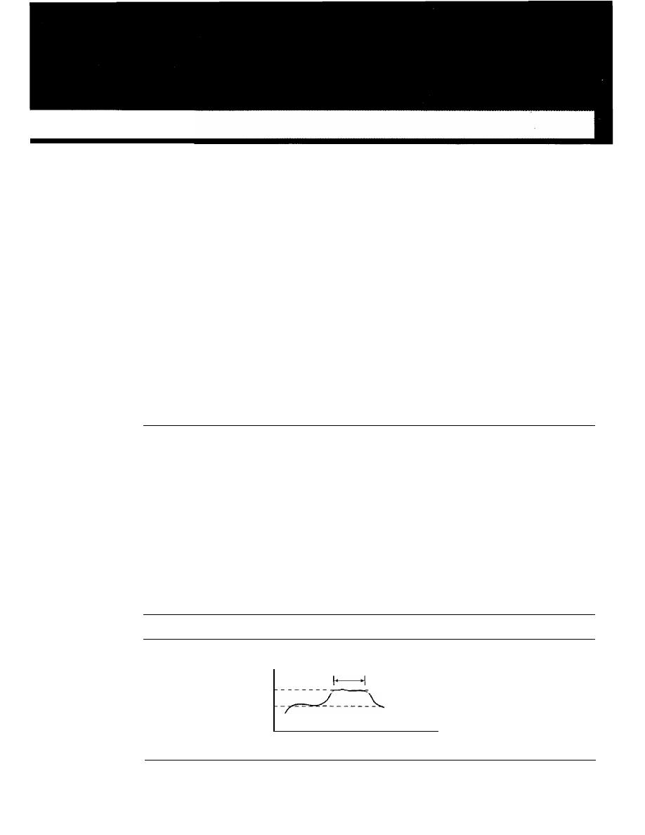
CHAPTER 24
Congestion Control and
Quality of Service
Congestion control and quality of service are two issues so closely bound together that
improving one means improving the other and ignoring one usually means ignoring the
other. Most techniques to prevent or eliminate congestion also improve the quality of
service in a network.
We have postponed the discussion of these issues until now because these are issues
related not to one layer, but to three: the data link layer, the network layer, and the
transport layer. We waited until now so that we can discuss these issues once instead of
repeating the subject three times. Throughout the chapter, we give examples of conges-
tion control and quality of service at different layers.
24.1
DATA TRAFFIC
The main focus of congestion control and quality of service is data traffic. In congestion
control we try to avoid traffic congestion. In quality of service, we try to create an
appropriate environment for the traffic. So, before talking about congestion control and
quality of service, we discuss the data traffic itself.
Traffic Descriptor
Traffic descriptors are qualitative values that represent a data flow. Figure 24.1 shows a
traffic flow with some of these values.
Figure 24.1
Traffic descriptors
Data rate
Maximum
burst size
-
-
-
-
-
-
-
Peak data rate
- - - - - Average data rate
Seconds
761

762
CHAPTER
24
CONGESTION CONTROL AND QUAliTY OF SERVICE
Average Data Rate
The
average data rate
is the number of bits sent during a period of time, divided by the
number of seconds in that period. We use the following equation:
Average data rate
=
amount of data
time
The average data rate is a very useful characteristic of traffic because it indicates the
average bandwidth needed by the traffic.
Peak Data Rate
The
peak data rate
defines the maximum data rate of the traffic. In Figure
24.1
it is the
maximum
y
axis value. The peak data rate is a very important measurement because
it indicates the peak bandwidth that the network needs for traffic to pass through without
changing its data flow.
Maximum Burst Size
Although the peak data rate is a critical value for the network, it can usually be ignored
if the duration of the peak value is very short. For example, if data are flowing steadily
at the rate of 1 Mbps with a sudden peak data rate of 2 Mbps for just 1 ms, the network
probably can handle the situation. However, if the peak data rate lasts 60
there may
be a problem for the network. The
maximum burst size
normally refers to the maximum
length of time the traffic is generated at the peak rate.
Effective Bandwidth
The
effective bandwidth
is the bandwidth that the network needs to allocate for the
flow of traffic. The effective bandwidth is a function of three values: average data rate,
peak data rate, and maximum burst size. The calculation of this value is very complex.
Traffic Profiles
For our purposes, a data flow can have one of the following traffic profiles: constant bit
rate, variable bit rate, or bursty as shown in Figure
24.2.
Constant Bit Rate
A
constant-bit-rate (CBR),
or a fixed-rate, traffic model has a data rate that does not
change. In this type of flow, the average data ratc and thc peak data rate are the same.
The maximum burst size is not applicable. This type of traffic is very easy for a network
to handle since it is predictable. The network knows in advance how much bandwidth to
allocate for this type of flow.
Variable Bit Rate
In the
variable-bit-rate (VBR)
category, the rate of the data flow changes in time, with
the changes smooth instead of sudden and sharp. In this type of flow, the average data
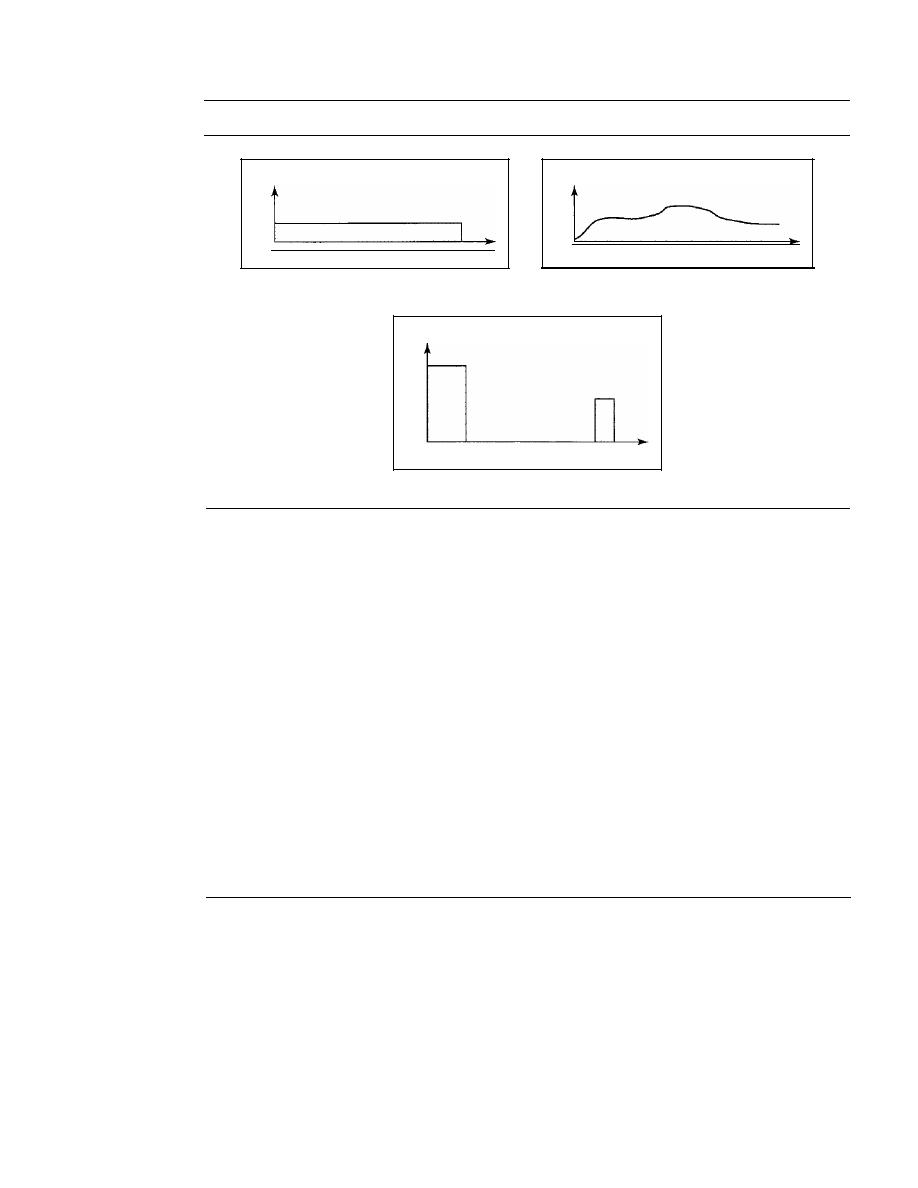
SECTION
24.2
CONGESTION
763
Figure 24.2
Three traffic profiles
Data rate
Time
a. Constant bit rate
Data rate
Data rate
Time
b. Variable bit rate
Time
c. Bursty
rate and the peak data rate are different. The maximum burst size is usually a small
value. This type of traffic is more difficult to handle than constant-bit-rate traffic, but it
normally does not need to be reshaped, as we will see later.
Bursty
In the
bursty data category, the data rate changes suddenly in a very short time.
It
may jump from zero, for example, to 1 Mbps in a few microseconds and vice versa.
It
may also remain at this value for a while. The average bit rate and the peak bit rate are
very different values in this type of flow. The maximum burst size is significant. This
is the most difficult type of traffic for a network to handle because the profile is very
unpredictable. To handle this type of traffic, the network normally needs to reshape it,
using reshaping techniques, as we will see shortly. Bursty traffic is one of the main
causes of congestion in a network.
24.2
CONGESTION
An important issue in a packet-switched network is
congestion. Congestion in a network
may occur if the
load on the network-the number of packets sent to the network-is
greater than the capacity of the network-the number of packets a network can handle.
Congestion control refers to the mechanisms and techniques to control the congestion
and keep the load below the capacity.
We may ask why there is congestion on a network. Congestion happens in any
system that involves waiting. For example, congestion happens on a freeway because
any abnonnality in the flow, such as an accident during rush hour, creates blockage.
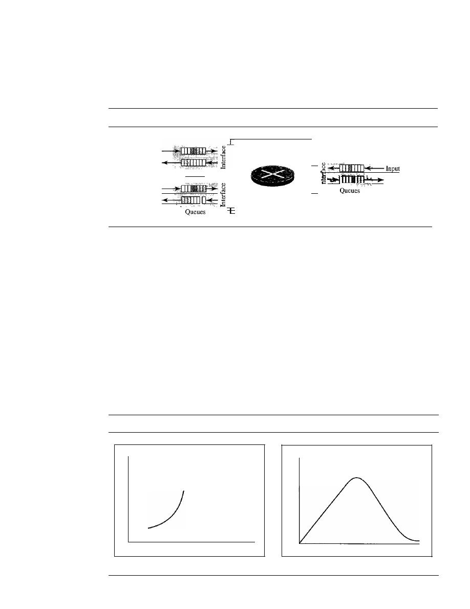
Input
Output
764
CHAPTER
24
CONGESTION CONTROL AND QUALITY OF SERVICE
Congestion in a network or internetwork occurs because routers and switches have
queues-buffers that hold the packets before and after processing. A router, for example,
has an input queue and an output queue for each interface. When a packet arrives at the
incoming interface, it undergoes three steps before departing, as shown in Figure 24.3.
Figure 24.3
Queues in a router
1
Queues
I
Output
Input
J-
Output
_
1. The packet is put at the end of the input queue while waiting to be checked.
2. The processing module of the router removes the packet from the input queue once
it reaches the front of the queue and uses its routing table and the destination
address to find the route.
3. The packet is put in the appropriate output queue and waits its tum to be sent.
We need to be aware of two issues. First, if the rate of packet arrival is higher than the
packet processing rate, the input queues become longer and longer. Second, if the packet
departure rate is less than the packet processing rate, the output queues become longer
and longer.
Network Performance
Congestion control involves two factors that measure the performance of a network: delay
and throughput. Figure 24.4 shows these two performance measures as function of load.
Figure 24.4
Packet delay and throughput as functions of load
Delay
Throughput
Capacity
No congestion area Congestion area
Capacity
Load
No congestion
area
Congestion area
Load
a. Delay as a function ofload
b. Throughput as a function of load
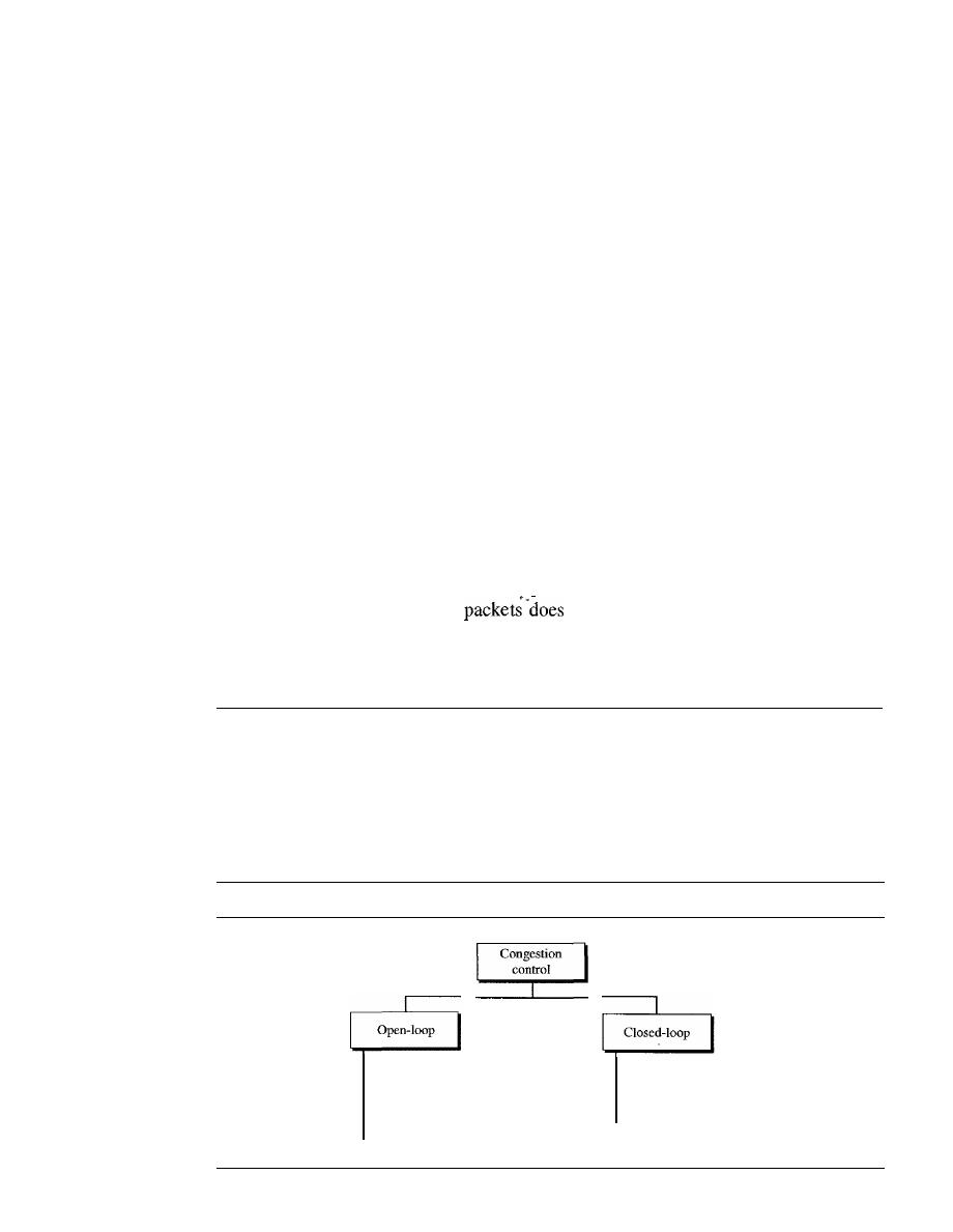
SECTION
24.3
CONGESTION CONTROL
765
Delay Versus Load
Note that when the load is much less than the capacity of the network, the delay is at a
minimum. This minimum delay is composed of propagation delay and processing delay,
both of which are negligible. However, when the load reaches the network capacity, the
delay increases sharply because we now need to add the waiting time in the queues (for all
routers in the path) to the total delay. Note that the delay becomes infinite when the load is
greater than the capacity.
If
this is not obvious, consider the size of the queues when
almost no packet reaches the destination, or reaches the destination with infinite delay; the
queues become longer and longer. Delay has a negative effect on the load and conse-
quently the congestion. When a packet is delayed, the source, not receiving the acknowl-
edgment, retransmits the packet, which makes the delay, and the congestion, worse.
Throughput Versus Load
We defined throughput in Chapter 3 as the number of bits passing through a point in a
second. We can extend that definition from bits to packets and from a point to a net-
work. We can define throughput in a network as the number of packets passing
through the network in a unit of time. Notice that when the load is below the capacity
of the network, the throughput increases proportionally with the load. We expect the
throughput to remain constant after the load reaches the capacity, but instead the
throughput declines sharply. The reason is the discarding of packets by the routers.
When the load exceeds the capacity, the queues become full and the routers have to dis-
card some packets. Discarding
not reduce the number of packets in the
network because the sources retransmit the packets, using time-out mechanisms, when
the packets do not reach the destinations.
24.3
CONGESTION CONTROL
Congestion control refers to techniques and mechanisms that can either prevent conges-
tion, before it happens, or remove congestion, after it has happened. In general, we can
divide congestion control mechanisms into two broad categories: open-loop congestion
control (prevention) and closed-loop congestion control (removal) as shown in Figure 24.5.
Figure 24.5
Congestion control categories
Retransmission policy
Window policy
Acknowledgment policy
Discarding policy
Admission policy
Back pressure
Choke packet
Implicit signaling
Explicit signaling

766
CHAPTER
24
CONGESTION CONTROL AND QUALITY OF SERVICE
Open-Loop Congestion Control
In open-loop congestion control, policies are applied to prevent congestion before it
happens. In these mechanisms, congestion control is handled by either the source or the
destination. We give a brief list of policies that can prevent congestion.
Retransmission Policy
Retransmission is sometimes unavoidable.
If
the sender feels that a sent packet is lost
or corrupted, the packet needs to be retransmitted. Retransmission in general may
increase congestion in the network. However, a good retransmission policy can prevent
congestion. The retransmission policy and the retransmission timers must be designed
to optimize efficiency and at the same time prevent congestion. For example, the
retransmission policy used by TCP (explained later) is designed to prevent or alleviate
congestion.
Window Policy
The type of window at the sender may also affect congestion. The Selective Repeat
window is better than the Go-Back-N window for congestion control. In the Go-Back-N
window, when the timer for a packet times out, several packets may be resent, although
some may have arrived safe and sound at the receiver. This duplication may make the
congestion worse. The Selective Repeat window, on the other hand, tries to send the
specific packets that have been lost or corrupted.
Acknowledgment Policy
The acknowledgment policy imposed by the receiver may also affect congestion.
If
the
receiver does not acknowledge every packet it receives, it may slow down the sender
and help prevent congestion. Several approaches are used in this case. A receiver may
send an acknowledgment only if it has a packet to be sent or a special timer expires. A
receiver may decide to acknowledge only N packets at a time. We need to know that
the acknowledgments are also part of the load in a network. Sending fewer acknowl-
edgments means imposing less load on the network.
Discarding Policy
A good discarding policy by the routers may prevent congestion and at the same time
may not harm the integrity of the transmission. For example, in audio transmission, if
the policy is to discard less sensitive packets when congestion is likely to happen, the
quality of sound is still preserved and congestion is prevented or alleviated.
Admission Policy
An admission policy, which is a quality-of-service mechanism, can also prevent conges-
tion in virtual-circuit networks. Switches in a flow first check the resource requirement
of a flow before admitting it to the network. A router can deny establishing a virtual-
circuit connection if there is congestion in the network or if there is a possibility of future
congestion.
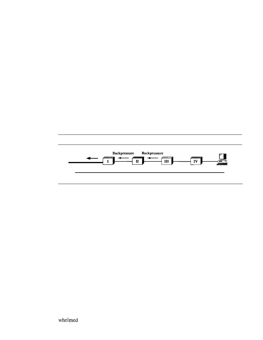
SECTION
24.3
CONGESTION CONTROL
767
Closed-Loop Congestion Control
Closed-loop congestion control mechanisms
try
to alleviate congestion after it hap-
pens. Several mechanisms have been used by different protocols. We describe a few of
them here.
Backpressure
The technique of
backpressure refers to a congestion control mechanism in which a
congested node stops receiving data from the immediate upstream node or nodes. This
may cause the upstream node or nodes to become congested, and they, in turn, reject
data from their upstream nodes or nodes. And so on. Backpressure is a node-to-node
congestion control that starts with a node and propagates, in the opposite direction of
data flow, to the source. The backpressure technique can be applied only to virtual circuit
networks, in which each node knows the upstream node from which a flow of data is
corning. Figure 24.6 shows the idea of backpressure.
Figure 24.6
Backpressure method for alleviating congestion
Source
Backpressure
Dataflow
Congestion
Destination
Node III in the figure has more input data than it can handle. It drops some packets
in its input buffer and informs node II to slow down. Node II, in turn, may be congested
because it is slowing down the output flow of data.
If
node II is congested, it informs
node I to slow down, which in turn may create congestion.
If
so, node I informs the
source of data to slow down. This, in time, alleviates the congestion. Note that the
pressure
on node III is moved backward to the source to remove the congestion.
None of the virtual-circuit networks we studied in this book use backpressure. It
was, however, implemented in the first virtual-circuit network, X.25. The technique
cannot be implemented in a datagram network because in this type of network, a node
(router) does not have the slightest knowledge of the upstream router.
Choke Packet
A
choke packet is a packet sent by a node to the source to inform it of congestion.
Note the difference between the backpressure and choke packet methods. In backpres-
sure, the warning is from one node to its upstream node, although the warning may
eventually reach the source station. In the choke packet method, the warning is from the
router, which has encountered congestion, to the source station directly. The inter-
mediate nodes through which the packet has traveled are not warned. We have seen
an example of this type of control in ICMP. When a router in the Internet is over-
with IP datagrams, it may discard some of them; but it informs the source
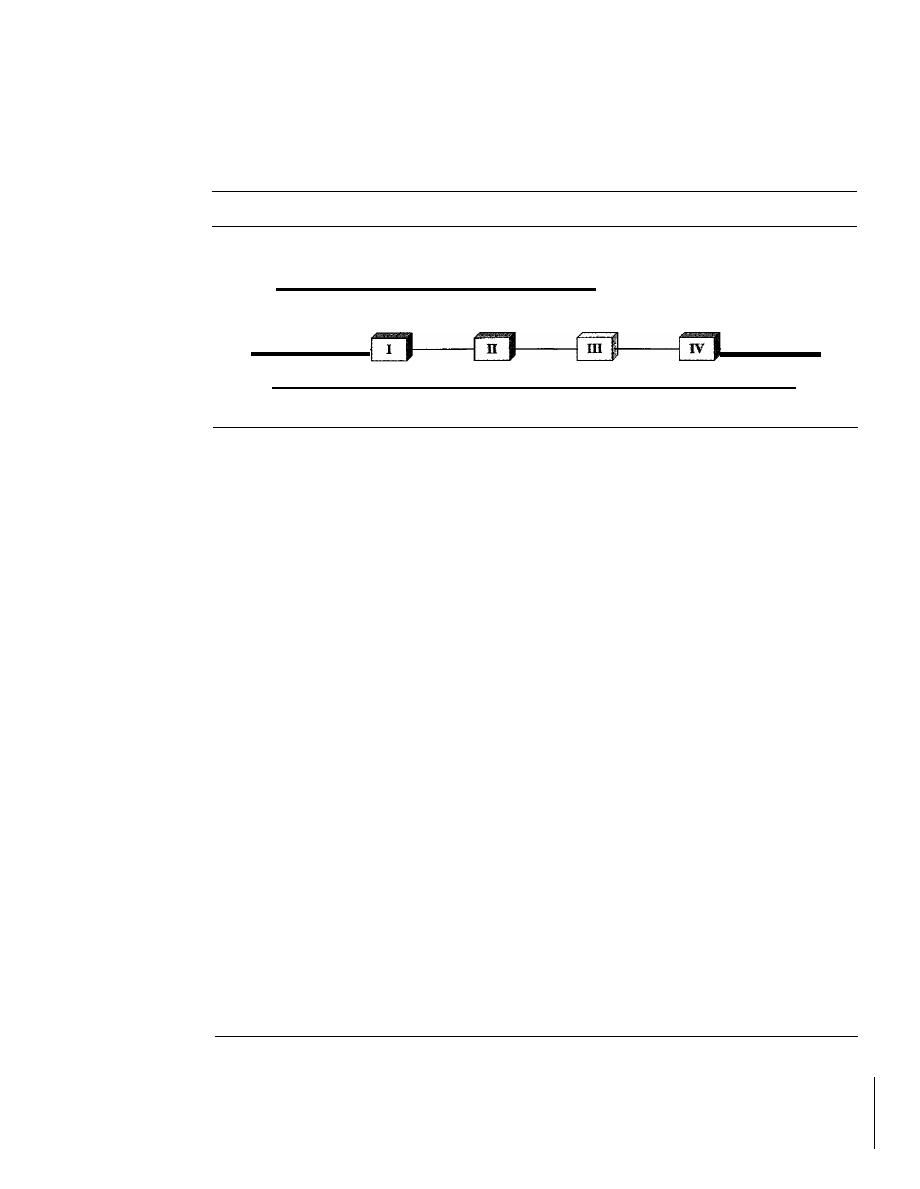
768
CHAPTER
24
CONGESTION CONTROL AND QUALITY OF SERVICE
host, using a source quench ICMP message. The warning message goes directly to the
source station; the intermediate routers, and does not take any action. Figure 24.7
shows the idea of a choke packet.
Figure 24.7
Choke packet
Choke
packet
Source
Congestion
Dataflow
Destination
Implicit Signaling
In implicit signaling, there is no communication between the congested node or nodes
and the source. The source guesses that there is a congestion somewhere in the network
from other symptoms. For example, when a source sends several packets and there is
no acknowledgment for a while, one assumption is that the network is congested. The
delay in receiving an acknowledgment is interpreted as congestion in the network; the
source should slow down. We will see this type of signaling when we discuss TCP
congestion control later in the chapter.
Explicit Signaling
The node that experiences congestion can explicitly send a signal to the source or desti-
nation. The explicit signaling method, however, is different from the choke packet
method. In the choke packet method, a separate packet is used for this purpose; in the
explicit signaling method, the signal is included in the packets that carry data. Explicit
signaling, as we will see in Frame Relay congestion control, can occur in either the
forward or the backward direction.
Backward Signaling
A bit can be set in a packet moving in the direction opposite
to the congestion. This bit can warn the source that there is congestion and that it needs
to slow down to avoid the discarding of packets.
Forward Signaling
A bit can be set in a packet moving in the direction of the
congestion. This bit can warn the destination that there is congestion. The receiver in
this case can use policies, such as slowing down the acknowledgments, to alleviate the
i
congestion.
24.4
TWO EXAMPLES
To better understand the concept of congestion control, let us give two examples: one in
TCP and the other in Frame Relay.

SECTION
24.4
1WO EXAMPLES
769
Congestion Control in TCP
We discussed TCP in Chapter 23. We now show how TCP uses congestion control to
avoid congestion or alleviate congestion in the network.
Congestion Window
In
Chapter 23, we talked about flow control and tried to discuss solutions when the receiver
is overwhelmed with data. We said that the sender window size is determined by the avail-
able buffer space in the receiver (rwnd). In other words, we assumed that it is only the
receiver that can dictate to the sender the size of the sender's window. We totally ignored
another entity here-the network. If the network cannot deliver the data as fast as they are
created by the sender, it must tell the sender to slow down.
In
other words, in addition to
the receiver, the network is a second entity that determines the size of the sender's window.
Today, the sender's window size is determined not only by the receiver but also by
congestion in the network.
The sender has two pieces of information: the receiver-advertised window size and
the congestion window size. The actual size of the window is the minimum of these two.
Actual window
minimum (rwnd, cwnd)
We show shortly how the size of the congestion window (cwnd) is determined.
Congestion
Policy
TCP's general policy for handling congestion is based on three phases: slow start, con-
gestion avoidance, and congestion detection. In the slow-start phase, the sender starts
with a very slow rate of transmission, but increases the rate rapidly to reach a threshold.
When the threshold is reached, the data rate is reduced to avoid congestion. Finally if
congestion is detected, the sender goes back to the slow-start or congestion avoidance
phase based on how the congestion is detected.
Slow Start: Exponential Increase
One of the algorithms used in TCP congestion
control is called slow start. This algorithm is based on the idea that the size of the con-
gestion window (cwnd) starts with one maximum segment size (MSS). The MSS is
determined during connection establishment by using an option of the same name. The
size of the window increases one MSS each time an acknowledgment is received. As the
name implies, the window starts slowly, but grows exponentially. To show the idea, let us
look at Figure 24.8. Note that we have used three simplifications to make the discussion
more understandable. We have used segment numbers instead of byte numbers (as though
each segment contains only 1 byte). We have assumed that rwnd is much higher than
cwnd,
so that the sender window size always equals cwnd. We have assumed that each
segment is acknowledged individually.
The sender starts with cwnd
=
1 MSS. This means that the sender can send only
one segment. After receipt of the acknowledgment for segment 1, the size of the
congestion window is increased by 1, which means that cwnd is now 2. Now two
more segments can be sent. When each acknowledgment is received, the size of
window is increased by 1 MSS. When all seven segments are acknowledged,
cwnd
=
8.
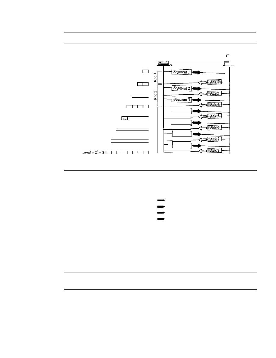
770
CHAPTER
24
CONGESTION CONTROL AND QUALITY OF SERVICE
Figure 24.8
Slow start, exponential increase
Rnd: Round of transmission
cwnd=20=
1
cwnd
=
2
1
=
2
cwnd
=
2
2
=
4
Sender
Time
Segment 4
Segment
5
Segment 6
Segment
7
Receiver
-
Time
If
we look at the size of
cwnd
in terms of rounds (acknowledgment of the whole
window of segments), we find that the rate is exponential as shown below:
Start
cwnd=l
After round 1
cwnd=2
1
=2
After round 2
cwnd=2
2
=4
After round 3
cwnd=2
3
=8
We need to mention that if there is delayed ACKs, the increase in the size of the
window is less than power of 2.
Slow start cannot continue indefinitely. There must be a threshold to stop this
phase. The sender keeps track of a variable named
ssthresh
(slow-start threshold).
When the size of window in bytes reaches this threshold, slow start stops and the next
phase starts. In most implementations the value of
ssthresh
is 65,535 bytes.
In the slow-start algorithm, the size of the congestion window
increases exponentially until it reaches a threshold.
Congestion Avoidance: Additive Increase
If
we start with the slow-start algorithm,
the size of the congestion window increases exponentially. To avoid congestion before
it happens, one must slow down this exponential growth. TCP defines another algo-
rithm called congestion avoidance, which undergoes an additive increase instead of
an exponential one. When the size of the congestion window reaches the slow-start
threshold, the slow-start phase stops and the additive phase begins. In this algorithm,
each time the whole window of segments is acknowledged (one round), the size of the
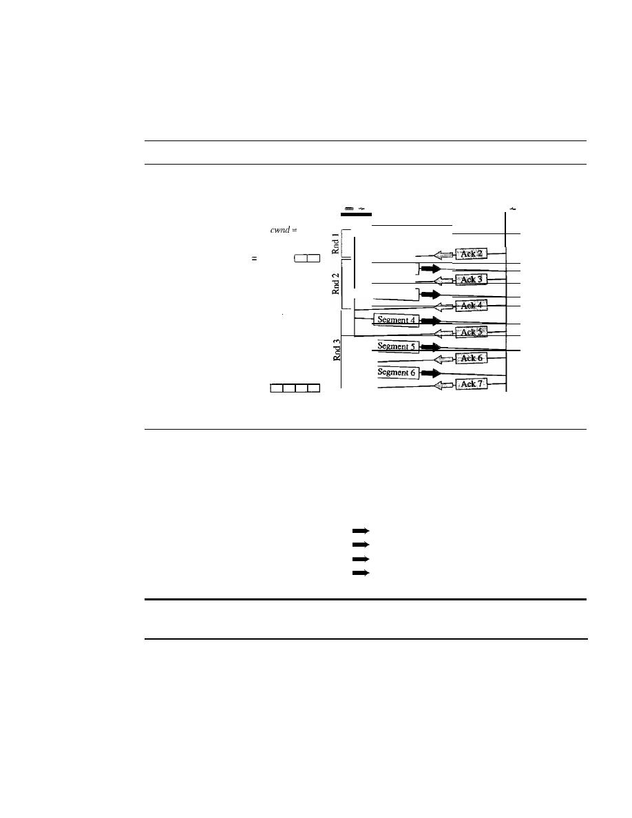
SECTION
24.4
1WO EXAMPLES
771
congestion window is increased by 1. To show the idea, we apply this algorithm to the same
scenario as slow start, although we will see that the congestion avoidance algorithm usually
starts when the size of the window is much greater than 1. Figure 24.9 shows the idea.
Figure 24.9
Congestion avoidance, additive increase
Rnd: Round of transmission
Sender
Receiver
-
1 0
Segment 1
cwnd
1
+
1
=
2
Segment 2
Segment 3
cwnd
=
2
+
1
=
3 I
Segment 5
cwnd
=
3
+
1
=
4
Time
Time
In this case, after the sender has received acknowledgments for a complete window
size of segments, the size of the window is increased by one segment.
If we look at the size of cwnd in terms of rounds, we find that the rate is additive as
shown below:
Start
After round 1
After round 2
After round 3
cwnd=l
cwnd=
1+ 1 =2
cwnd=2+
1 =3
cwnd=3+
1 =4
In the congestion avoidance algorithm, the size of the congestion
window increases additively until congestion
is
detected.
Congestion Detection: Multiplicative Decrease
If
congestion occurs, the congestion
window size must be decreased. The only way the sender can guess that congestion has
occurred is by the need to retransmit a segment. However, retransmission can occur in
one of two cases: when a timer times out or when three ACKs are received. In both
cases, the size of the threshold is dropped to one-half, a multiplicative decrease. Most
TCP implementations have two reactions:
I.
If a time-out occurs, there is a stronger possibility of congestion; a segment has
probably been dropped in the network, and there is no news about the sent segments.
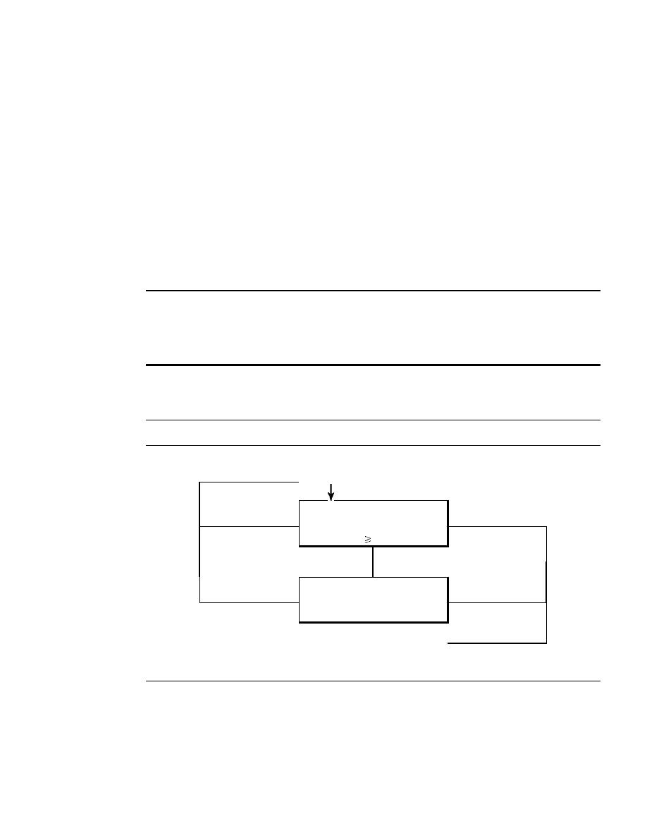
772
CHAPTER
24
CONGESTION CONTROL AND QUALITY OF SERVICE
In this case TCP reacts strongly:
a.
It
sets the value of the threshold to one-half of the current window size.
b.
It
sets
cwnd to the size of one segment.
c. It starts the slow-start phase again.
2.
If
three ACKs are received, there is a weaker possibility of congestion; a segment
may have been dropped, but some segments after that may have arrived safely since
three ACKs are received. This is called fast transmission and fast recovery. In this
case, TCP has a weaker reaction:
a.
It
sets the value of the threshold to one-half of the current window size.
b. It sets
cwnd to the value of the threshold (some implementations add three
segment sizes to the threshold).
c.
It
starts the congestion avoidance phase.
An implementations reacts to congestion detection in one of the following ways:
o
If
detection is by time-out, a new
slow-start phase starts.
o
If
detection is by three ACKs, a new
congestion avoidance phase starts.
Summary
In Figure 24.10, we summarize the congestion policy of TCP and the rela-
tionships between the three phases.
Figure 24.10
TCP congestion policy summary
ssthresh
=
112 window
cwnd= 1 MSS
Time-out
Slow start
3 ACKs
Congestion
Congestion
cwnd
ssthresh
ssthresh
=
112 window
cwnd
=
ssthresh
Time-out
Congestion
3 ACKs
Congestion
avoidance
Congestion
t
ssthresh
=
112 wmdow
cwnd
=
ssthresh
We give an example in Figure 24.11. We assume that the maximum window size is
32 segments. The threshold is set to
16
segments (one-half of the maximum window
size). In the
slow-start phase the window size starts from
1
and grows exponentially
until it reaches the threshold. After it reaches the threshold, the
congestion avoidance
(additive increase) procedure allows the window size to increase linearly until a time-
out occurs or the maximum window size is reached. In Figure 24.11, the time-out occurs
when the window size is 20. At this moment, the
multiplicative decrease procedure takes
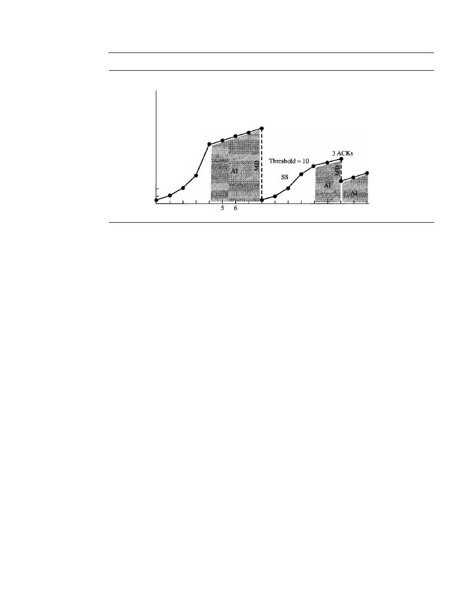
SECTION 24.4
TWO EXAMPLES
773
Figure 24.11
Congestion example
cwnd
58
2 3 4
SS: Slow start
AI: Additive increase
MD:
Multiplicative decrease
Time-out
7
8
9
10
11
12
13
14
15
16 Rounds
26
24
22
20
18
Threshold
=
16
16
14
12
10
08
06
04
02
over and reduces the threshold to one-half of the previous window size. The previous
window size was 20 when the time-out happened so the new threshold is now 10.
TCP moves to slow start again and starts with a window size of 1, and TCP moves
to additive increase when the new threshold is reached. When the window size is 12, a
three-ACKs event happens. The multiplicative decrease procedure takes over again.
The threshold is set to 6 and TCP goes to the additive increase phase this time.
It
remains in this phase until another time-out or another three ACKs happen.
Congestion Control in Frame Relay
Congestion in a Frame Relay network decreases throughput and increases delay. A high
throughput and low delay are the main goals of the Frame Relay protocol. Frame Relay
does not have flow control. In addition, Frame Relay allows the user to transmit bursty
data. This means that a Frame Relay network has the potential to be really congested
with traffic, thus requiring congestion control.
Congestion Avoidance
For congestion avoidance, the Frame Relay protocol uses 2 bits in the frame to explicitly
warn the source and the destination of the presence of congestion.
BECN
The
backward explicit congestion notification (BECN)
bit warns the sender of
congestion in the network. One might ask how this is accomplished since the frames are
traveling away from the sender. In fact, there are two methods: The switch can use response
frames from the receiver (full-duplex mode), or else the switch can use a predefined connec-
tion (DLCI
=
1023) to send special frames for this specific purpose. The sender can respond
to
this warning by simply reducing the data rate. Figure 24.12 shows the use ofBECN.
FECN
The
forward explicit congestion notification (FECN)
bit is used to warn
the receiver of congestion in the network. It might appear that the receiver cannot do
anything to relieve the congestion. However, the Frame Relay protocol assumes that the
sender and receiver are communicating with each other and are using some type of flow
control at a higher level. For example, if there is an acknowledgment mechanism at this
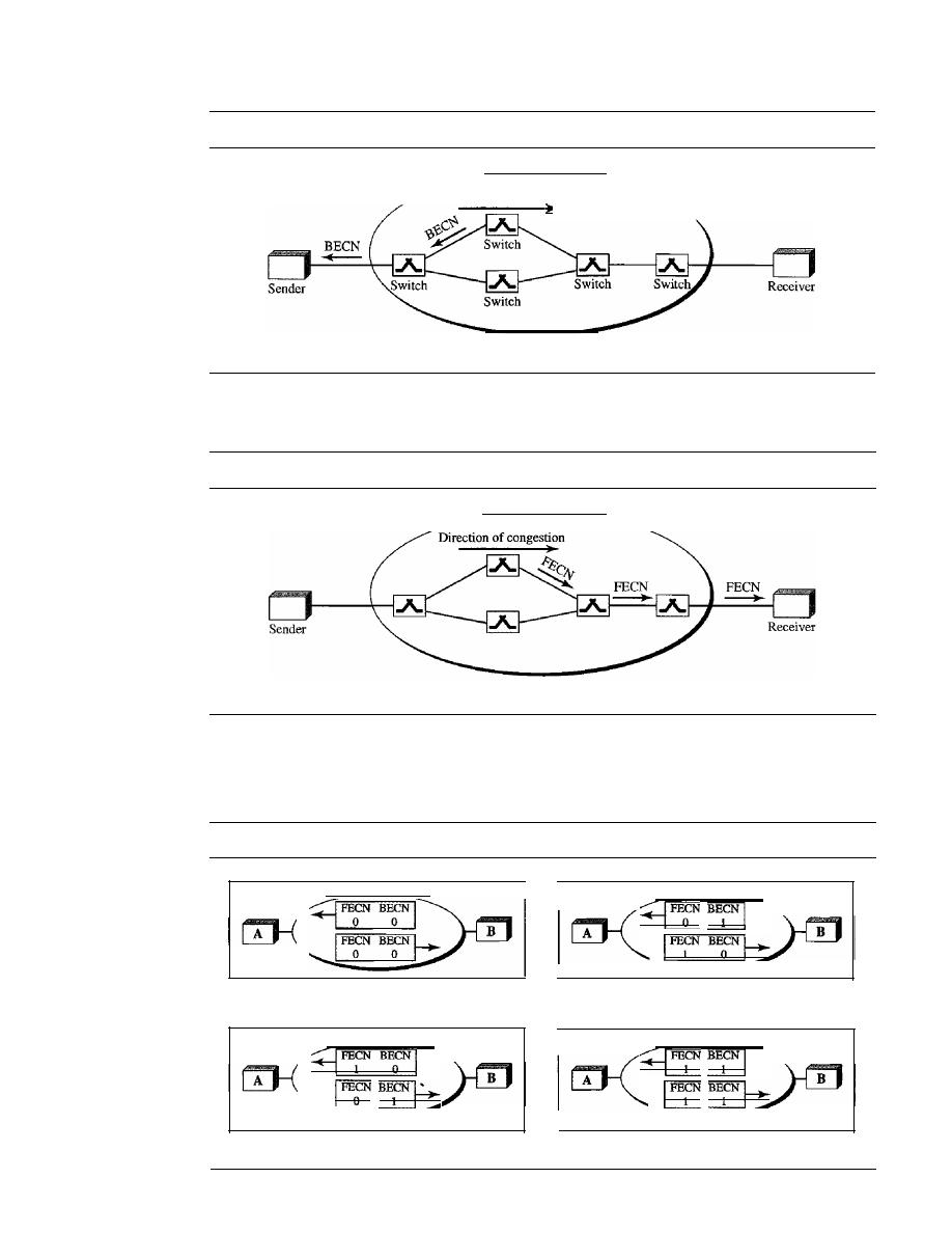
774
CHAPTER
24
CONGESTION CONTROL AND QUALITY OF SERVICE
Figure 24.12
BECN
Direction of congestion
Frame Relay network
higher level, the receiver can delay the acknowledgment, thus forcing the sender to
slow down. Figure 24.13 shows the use ofFECN.
Figure 24.13
FECN
Frame Relay network
When two endpoints are communicating using a Frame Relay network, four situa-
tions may occur with regard to congestion. Figure 24.14 shows these four situations
and the values of FECN and BECN.
Figure 24.14
Four cases ofcongestion
a. No congestion
b. Congestion in the direction A-B
c. Congestion in the direction B-A
d. Congestion in both directions
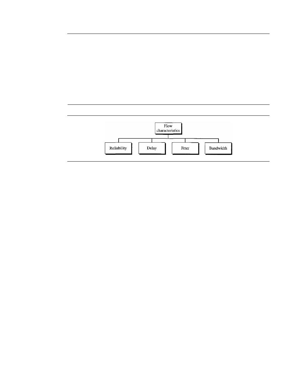
SECTION
24.5
QUALITY OF SERVICE
775
24.5
QUALITY OF SERVICE
Quality of service (QoS) is an internetworking issue that has been discussed more than
defined. We can informally define quality of service as something a flow seeks to attain.
Flow Characteristics
Traditionally, four types of characteristics are attributed to a flow: reliability, delay,
jitter, and bandwidth, as shown in Figure 24.15.
Figure 24.15
Flow characteristics
Reliability
Reliability is a characteristic that a flow needs. Lack of reliability means losing a
packet or acknowledgment, which entails retransmission. However, the sensitivity of
application programs to reliability is not the same. For example, it is more important
that electronic mail, file transfer, and Internet access have reliable transmissions than
telephony or audio conferencing.
Delay
Source-to-destination delay is another flow characteristic. Again applications can tolerate
delay in different degrees.
In
this case, telephony, audio conferencing, video conferenc-
ing, and remote log-in need minimum delay, while delay in file transfer or e-mail is less
important.
Jitter
Jitter is the variation in delay for packets belonging to the same flow. For example, if
four packets depart at times 0, 1, 2, 3 and arrive at 20, 21, 22, 23, all have the same
delay, 20 units of time. On the other hand,
if
the above four packets arrive at 21, 23, 21,
and 28, they will have different delays: 21,22, 19, and 24.
For applications such as audio and video, the first case is completely acceptable;
the second case is not. For these applications, it does not matter if the packets arrive
with a short or long delay as long as the delay is the same for all packets. For this appli-
cation, the second case is not acceptable.
Jitter is defined as the variation in the packet delay. High jitter means the difference
between delays is large; low jitter means the variation is small.
In Chapter 29, we show how multimedia communication deals with jitter.
If
the
jitter is high, some action is needed in order to use the received data.
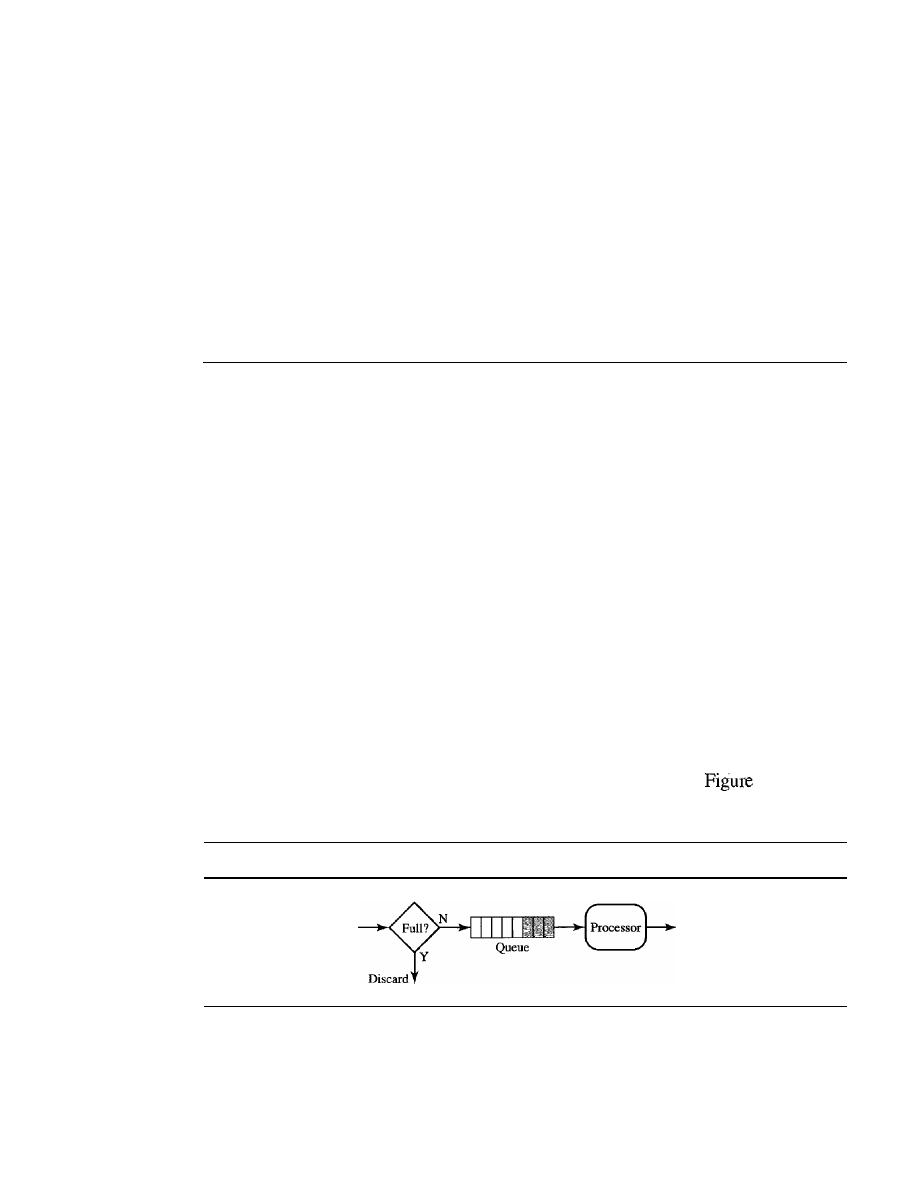
776
CHAPTER
24
CONGEST/ON CONTROL AND QUALITY OF SERVICE
Bandwidth
Different applications need different bandwidths. In video conferencing we need to
send millions of bits per second to refresh a color screen while the total number of bits
in an e-mail may not reach even a million.
Flow Classes
Based on the flow characteristics, we can classify flows into groups, with each group
having similar levels of characteristics. This categorization is not formal or universal;
some protocols such as ATM have defined classes, as we will see later.
24.6
lECHNIQUES TO IMPROVE QoS
In
Section 24.5 we tried to define QoS in terms of its characteristics. In this section, we
discuss some techniques that can be used to improve the quality of service. We briefly
discuss four common methods: scheduling, traffic shaping, admission control, and
resource reservation.
Scheduling
Packets from different flows arrive at a switch or router for processing. A good scheduling
technique treats the different flows in a fair and appropriate manner. Several scheduling
techniques are designed to improve the quality of service. We discuss three of them here:
FIFO queuing, priority queuing, and weighted fair queuing.
FIFO Queuing
In
first-in, first-out (FIFO) queuing,
packets wait in a buffer (queue) until the node
(router or switch) is ready to process them.
If
the average arrival rate is higher than the
average processing rate, the queue will fill up and new packets will be discarded. A FIFO
queue is familiar to those who have had to wait for a bus at a bus stop.
24.16 shows
a conceptual view of a FIFO queue.
Figure 24.16
FIFO queue
Arrival
Departure
Priority Queuing
In
priority queuing,
packets are first assigned to a priority class. Each priority class has
its own queue. The packets in the highest-priority queue are processed first. Packets in
the lowest-priority queue are processed last. Note that the system does not stop serving
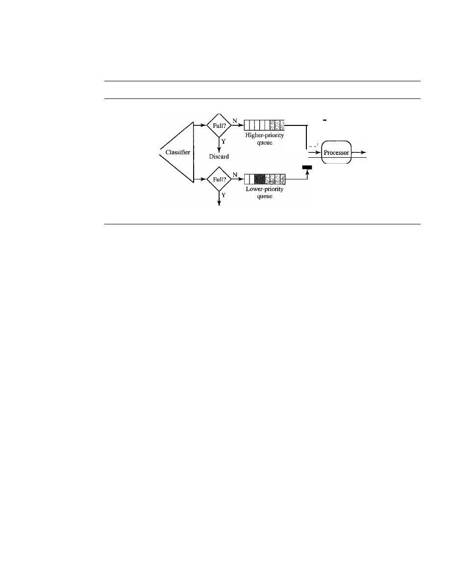
SECTION
24.6
TECHNIQUES TO IMPROVE QoS
777
a queue until it is empty. Figure 24.17 shows priority queuing with two priority levels
(for simplicity).
Figure 24.17
Priority queuing
The switch turns to the other
1-
queue when the current one
:
is empty.
I
I
Arrival
Departure
Discard
A priority queue can provide better QoS than the FIFO queue because higher-
priority traffic, such as multimedia, can reach the destination with less delay. However,
there is a potential drawback.
If
there is a continuous flow in a high-priority queue, the
packets in the lower-priority queues will never have a chance to be processed. This is a
condition called starvation.
Weighted Fair Queuing
A better scheduling method is weighted fair queuing. In this technique, the packets are
still assigned to different classes and admitted to different queues. The queues, how-
ever, are weighted based on the priority of the queues; higher priority means a higher
weight. The system processes packets in each queue in a round-robin fashion with the
number of packets selected from each queue based on the corresponding weight. For
example, if the weights are 3, 2, and 1, three packets are processed from the first queue,
two from the second queue, and one from the third queue.
If
the system does not
impose priority on the classes, all weights can be equaL In this way, we have fair queuing
with priority. Figure 24.18 shows the technique with three classes.
Traffic Shaping
Traffic shaping is a mechanism to control the amount and the rate of the traffic sent to
the network. Two techniques can shape traffic: leaky bucket and token bucket.
Leaky Bucket
If a bucket has a small hole at the bottom, the water leaks from the bucket at a constant rate
as long as there is water in the bucket. The rate at which the water leaks does not depend
on the rate at which the water is input to the bucket unless the bucket is empty. The input
rate can vary, but the output rate remains constant. Similarly, in networking, a technique
called leaky bucket can smooth out bursty traffic. Bursty chunks are stored in the bucket
and sent out at an average rate. Figure 24.19 shows a leaky bucket and its effects.
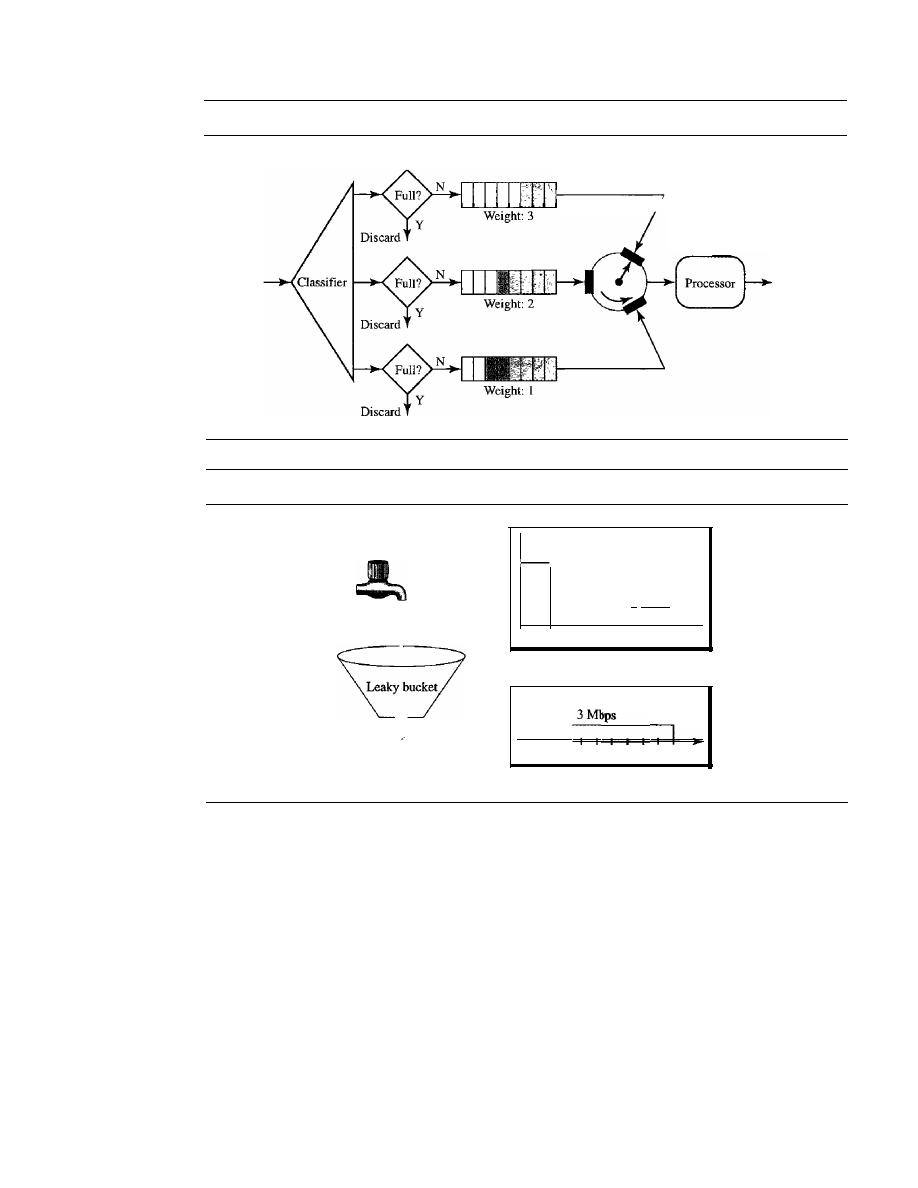
778
CHAPTER
24
CONGESTION CONTROL AND QUALITY OF SERVICE
Figure 24.18
Weighted fair queuing
Arrival
The tuming switch selects
3 packets from first queue,
then 2 packets from the second
queue, then
I
packet from the
third queue. The cycle repeats.
Departure
Figure 24.19
Leaky bucket
Bursty flow
12Mbps
2 Mbps
I
I
0 1 2 3 4 5 6 7 8 9 1 0
Bursty data
o
1--1-1
2 3 4 5 6 7 8 9 1 0
s
Fixed flow
Fixed-rate data
In the figure, we assume that the network has committed a bandwidth of 3 Mbps
for a host. The use of the leaky bucket shapes the input traffic to make it conform to this
commitment. In Figure 24.19 the host sends a burst of data at a rate of 12 Mbps for 2 s,
for a total of 24 Mbits of data. The host is silent for 5 s and then sends data at a rate of
2 Mbps for 3 s, for a total of 6 Mbits of data. In all, the host has sent 30 Mbits of data in
lOs. The leaky bucket smooths the traffic by sending out data at a rate of 3 Mbps during
the same 10 s. Without the leaky bucket, the beginning burst may have hurt the network
by consuming more bandwidth than is set aside for this host. We can also see that the
leaky bucket may prevent congestion. As an analogy, consider the freeway during rush
hour (bursty traffic). If, instead, commuters could stagger their working hours, congestion
o'n our freeways could be avoided.
A simple leaky bucket implementation is shown in Figure 24.20. A FIFO queue
holds the packets.
If
the traffic consists of fixed-size packets (e.g., cells in ATM
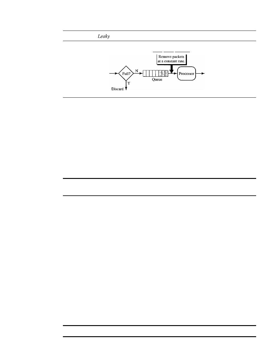
SECTION
24.6
TECHNIQUES TO IMPROVE QoS
779
Figure 24.20
bucket implementation
Leaky bucket algorithm
Arrival
Departure
networks), the process removes a fixed number of packets from the queue at each tick
of the clock. If the traffic consists of variable-length packets, the fixed output rate must
be based on the number of bytes or bits.
The following is an algorithm for variable-length packets:
1. Initialize a counter to
n
at the tick of the clock.
2.
If
n is greater than the size of the packet, send the packet and decrement the
counter by the packet size. Repeat this step until
n is smaller than the packet size.
3. Reset the counter and go to step 1.
A leaky bucket algorithm shapes bursty traffic into fixed-rate traffic by
averaging the data rate.
It
may drop the packets if the bucket is full.
Token Bucket
The leaky bucket is very restrictive.
It
does not credit an idle host. For example, if a
host is not sending for a while, its bucket becomes empty. Now if the host has bursty
data, the leaky bucket allows only an average rate. The time when the host was idle is
not taken into account. On the other hand, the token bucket algorithm allows idle
hosts to accumulate credit for the future in the form of tokens. For each tick of the
clock, the system sends
n
tokens to the bucket. The system removes one token for
every cell (or byte) of data sent. For example, if
n is 100 and the host is idle for 100 ticks,
the bucket collects 10,000 tokens. Now the host can consume all these tokens in one
tick with 10,000 cells, or the host takes 1000 ticks with 10 cells per tick. In other
words, the host can send bursty data as long as the bucket is not empty. Figure 24.21
shows the idea.
The token bucket can easily be implemented with a counter. The token is initial-
ized to zero. Each time a token is added, the counter is incremented by 1. Each time a
unit of data is sent, the counter is decremented by 1. When the counter is zero, the host
cannot send data.
The token bucket allows bursty traffic at a regulated maximum rate.
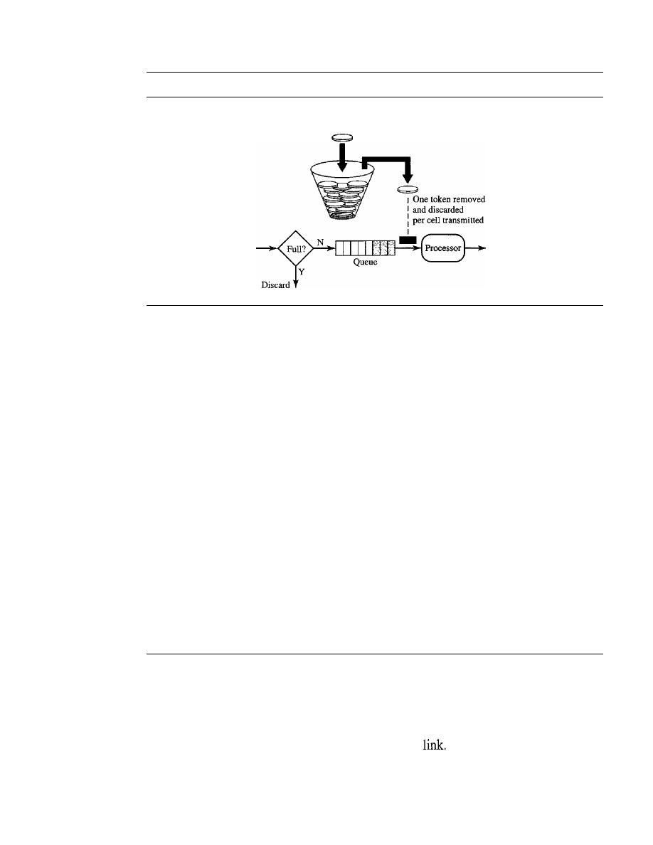
780
CHAPTER
24
CONGESTION CONTROL AND QUAliTY OF SERVICE
Figure 24.21
Token bucket
One token added
per tick
Arrival
Departure
Combining Token Bucket and Leaky Bucket
The two techniques can be combined to credit an idle host and at the same time regulate
the traffic. The leaky bucket is applied after the token bucket; the rate of the leaky bucket
needs to be higher than the rate of tokens dropped in the bucket.
Resource Reservation
A flow of data needs resources such as a buffer, bandwidth, CPU time, and so on. The
quality of service is improved if these resources are reserved beforehand. We discuss in
this section one QoS model called Integrated Services, which depends heavily on resource
reservation to improve the quality of service.
Admission Control
Admission control refers to the mechanism used by a router, or a switch, to accept or
reject a flow based on predefined parameters called flow specifications. Before a router
accepts a flow for processing, it checks the flow specifications to see if its capacity (in
terms of bandwidth, buffer size, CPU speed, etc.) and its previous commitments to other
flows can handle the new flow.
24.7
INTEGRATED SERVICES
Based on the topics in Sections 24.5 and 24.6, two models have been designed to provide
quality of service in the Internet: Integrated Services and Differentiated Services. Both
models emphasize the use of quality of service at the network layer (IP), although the
model can also be used in other layers such as the data
We discuss Integrated Services
in this section and Differentiated Service in Section 24.8.
As we learned in Chapter 20, IP was originally designed for best-effort delivery.
This means that every user receives the same level of services. This type of delivery

SECTION
24. 7
INTEGRATED SERVICES
781
does not guarantee the minimum of a service, such as bandwidth, to applications such
as real-time audio and video.
If
such an application accidentally gets extra bandwidth,
it may be detrimental to other applications, resulting in congestion.
Integrated Services,
sometimes called
IntServ,
is afiow-based QoS model, which
means that a user needs to create a flow, a kind of virtual circuit, from the source to the
destination and inform all routers of the resource requirement.
Integrated Services is a
QoS model designed for IP.
Signaling
The reader may remember that IP is a connectionless, datagram, packet-switching pro-
tocol. How can we implement a flow-based model over a connectionless protocol? The
solution is a signaling protocol to run over IP that provides the signaling mechanism for
making a reservation. This protocol is called
Resource Reservation Protocol (RSVP)
and will be discussed short!y.
Flow Specification
When a source makes a reservation, it needs to define a flow specification. A flow sped-
fication has two parts: Rspec (resource specification) and Tspec (traffic specification).
Rspec defines the resource that the flow needs to reserve (buffer, bandwidth, etc.). Tspec
defines the traffic characterization of the flow.
Admission
After a router receives the flow specification from an application, it decides to admit or
deny the service. The decision is based on the previous commitments of the router and
the current availability of the resource.
Service Classes
Two classes of services have been defined for Integrated Services: guaranteed service
and controlled-load service.
Guaranteed Service Class
This type of service is designed for real-time traffic that needs a guaranteed minimum
end-to-end delay. The end-to-end delay is the sum of the delays in the routers, the prop-
agation delay in the media, and the setup mechanism. Only the first, the sum of the
delays in the routers, can be guaranteed by the router. This type of service guarantees
that the packets will arrive within a certain delivery time and are not discarded if flow
traffic stays within the boundary of Tspec. We can say that guaranteed services are
quantitative services, in which the amount of end-to-end delay and the data rate must be
defined by the application.

782
CHAPTER
24
CONGESTION CONTROL AND QUALITY OF SERVICE
Controlled-Load Service Class
This type of service is designed for applications that can accept some delays, but are
sensitive to an overloaded network and to the danger of losing packets. Good examples
of these types of applications are file transfer, e-mail, and Internet access. The controlled-
load service is a qualitative type of service in that the application requests the possibility
of low-loss or no-loss packets.
RSVP
In the Integrated Services model, an application program needs resource reservation. As
we learned in the discussion of the IntServ model, the resource reservation is for a
flow.
This means that if we want to use IntServ at the IP level, we need to create a flow, a kind
of virtual-circuit network, out of the IP, which was originally designed as a datagram
packet-switched network. A virtual-circuit network needs a signaling system to set up the
virtual circuit before data traffic can start. The Resource Reservation Protocol (RSVP) is
a signaling protocol to help IP create a flow and consequently make a resource reserva-
tion. Before discussing RSVP, we need to mention that it is an independent protocol
separate from the Integrated Services model. It may be used
in
other models in the future.
Multicast Trees
RSVP is different from some other signaling systems we have seen before in that it is a
signaling system designed for multicasting. However, RSVP can be also used for uni-
casting because unicasting is just a special case of multicasting with only one member
in the multicast group. The reason for this design is to enable RSVP to provide resource
reservations for all kinds of traffic including multimedia which often uses multicasting.
Receiver-Based Reservation
In RSVP, the receivers, not the sender, make the reservation. This strategy matches the
other multicasting protocols. For example, in multicast routing protocols, the receivers,
not the sender, make a decision to join or leave a multicast group.
RSVP Messages
RSVP has several types of messages. However, for our purposes, we discuss only two
of them:
Path and Resv.
Path Messages
Recall that the receivers in a flow make the reservation in RSVP.
However, the receivers do not know the path traveled by packets before the reservation
is made. The path is needed for the reservation. To solve the problem, RSVP uses
Path
messages. A Path message travels from the sender and reaches all receivers in the multi-
cast path. On the way, a Path message stores the necessary information for the receivers.
A Path message is sent in a multicast environment; a new message is created when the
path diverges. Figure 24.22 shows path messages.
Resv Messages
After a receiver has received a Path message, it sends a
Resv
message.
The Resv message travels toward the sender (upstream) and makes a resource reservation
on the routers that support RSVP.
If
a router does not support RSVP on the path, it routes
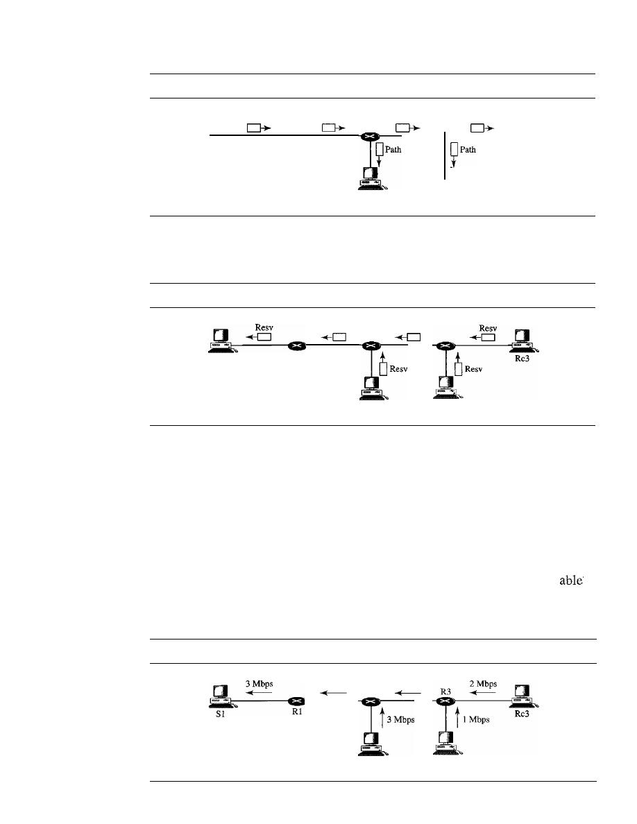
SECTION
24. 7
INTEGRATED SERVICES
783
Figure 24.22
Path messages
Path
81
Path
Path
ReI
Path
Rc2
Rc3
the packet based on the best-effort delivery methods we discussed before. Figure 24.23
shows the Resv messages.
Figure 24.23
Resv messages
81
Resv
Resv
Rcl
Rc2
Reservation Merging
In RSVP, the resources are not reserved for each receiver in a flow; the reservation is
merged.
In
Figure 24.24, Rc3 requests a 2-Mbps bandwidth while Rc2 requests a I-Mbps
bandwidth. Router R3, which needs to make a bandwidth reservation, merges the two
requests. The reservation is made for 2 Mbps, the larger of the two, because a 2-Mbps
input reservation can handle both requests. The same situation is true for R2. The
reader may ask why Rc2 and Rc3, both belonging to one single flow, request different
amounts of bandwidth. The answer is that, in a multimedia environment, different
receivers may handle different grades of quality. For example, Rc2 may be
to
receive video only at 1 Mbps (lower quality), while Rc3 may be able to receive video at
2 Mbps (higher quality).
Figure 24.24
Reservation merging
3Mbps
R2
Rcl
2 Mbps
Rc2
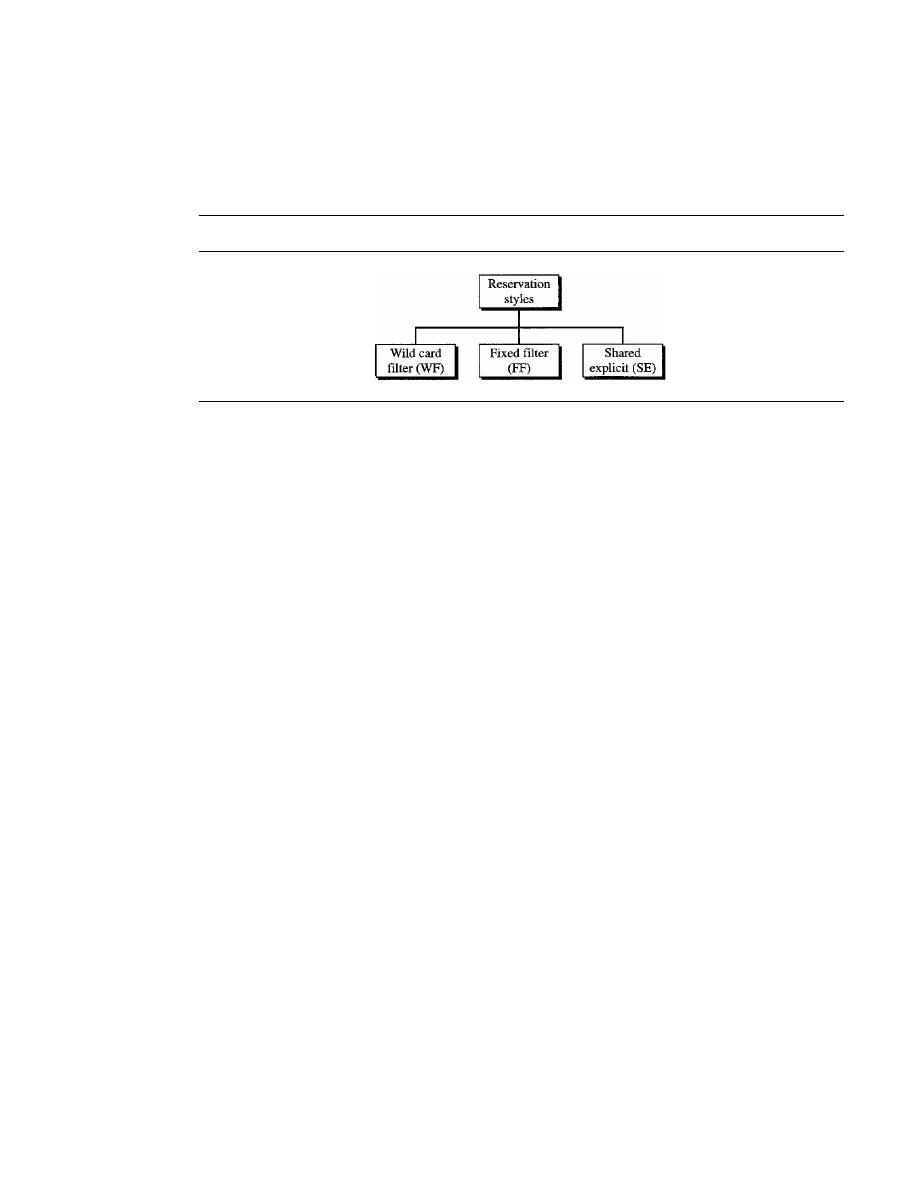
784
CHAPTER
24
CONGESTION CONTROL AND QUALITY OF SERVICE
Reservation Styles
When there is more than one flow, the router needs to make a reservation to accommodate
all of them. RSVP defines three types of reservation styles, as shown in Figure 24.25.
Figure 24.25
Reservation styles
Wild Card Filter Style
In this style, the router creates a single reservation for all
senders. The reservation is based on the largest request. This type of style is used when
the flows from different senders do not occur at the same time.
Fixed Filter Style
In this style, the router creates a distinct reservation for each flow.
This means that if there are n flows, n different reservations are made. This type of style
is used when there is a high probability that flows from different senders will occur at
the same time.
Shared Explicit Style
In this style, the router creates a single reservation which can
be shared by a set of flows.
Soft State
The reservation information (state) stored in every node for a flow needs to be refreshed
periodically. This is referred to as a soft state as compared to the hard state used in
other virtual-circuit protocols such as ATM or Frame Relay, where the information
about the flow is maintained until it is erased. The default interval for refreshing is
currently 30 s.
Problems with Integrated
Services
There are at least two problems with Integrated Services that may prevent its full imple-
mentation in the Internet: scalability and service-type limitation.
Scalability
The Integrated Services model requires that each router keep information for each flow.
As the Internet is growing every day, this is a serious problem.
Service-Type Limitation
The Integrated Services model provides only two types of services, guaranteed and
control-load. Those opposing this model argue that applications may need more than
these two types of services.

SECTION
24.8
DIFFERENTIATED SERVICES
785
24.8
DIFFERENTIATED SERVICES
Differentiated Services (DS or Diffserv) was introduced by the IETF (Internet Engi-
neering Task Force) to handle the shortcomings of Integrated Services. Two fundamental
changes were made:
1. The main processing was moved from the core of the network to the edge of the
network. This solves the scalability problem. The routers do not have to store
information about flows. The applications, or hosts, define the type of service they
need each time they send a packet.
2. The per-flow service is changed to per-class service. The router routes the packet
based on the class of service defined in the packet, not the flow. This solves the
service-type limitation problem. We can define different types of classes based on
the needs of applications.
Differentiated Services is a class-based QoS model designed for IP.
DS Field
In Diffserv, each packet contains a field called the DS field. The value of this field is set
at the boundary of the network by the host or the first router designated as the boundary
router. IETF proposes to replace the existing TOS (type of service) field in IPv4 or the
class field in IPv6 by the DS field, as shown in Figure 24.26.
Figure 24.26
DS field
DSCP
The DS field contains two subfields: DSCP and CU. The DSCP (Differentiated
Services Code Point) is a 6-bit subfield that defines the per-hop behavior (PHB). The
2-bit CU (currently unused) subfield is not currently used.
The Diffserv capable node (router) uses the DSCP 6 bits as an index to a table
defining the packet-handling mechanism for the current packet being processed.
Per-Hop Behavior
The Diffserv model defines per-hop behaviors (PHBs) for each node that receives a
packet. So far three PHBs are defined: DE PHB, EF PHB, and AF PHB.
DE PHB
The DE PHB (default PHB) is the same as best-effort delivery, which is
compatible with TOS.
EF PHB
The EF PHB (expedited forwarding PHB) provides the following services:
o
Low loss
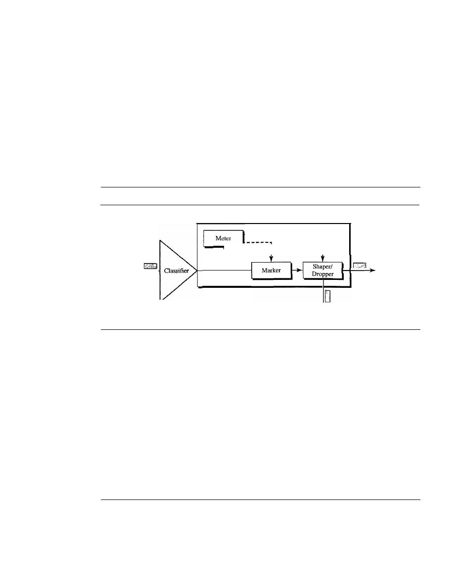
786
CHAPTER
24
CONGESTION CONTROL AND QUALITY OF SERVICE
o
Low latency
o
Ensured bandwidth
This is the same as having a virtual connection between the source and destination.
AF
PHB
The AF PHB (assured forwarding PHB) delivers the packet with a high
assurance as long as the class traffic does not exceed the traffic profile of the node. The
users of the network need to be aware that some packets may be discarded.
Traffic Conditioner
To implement Oiffserv, the OS node uses traffic conditioners such as meters, markers,
shapers, and droppers, as shown in Figure 24.27.
Figure
24.27
Traffic conditioner
Traffic conditioner
Input
-
......
Dropped
Output
Meters
The meter checks to see if the incoming flow matches the negotiated traffic
profile. The meter also sends this result to other components. The meter can use several
tools such as a token bucket to check the profile.
Marker
A marker can remark a packet that is using best-effort delivery (OSCP:
000000) or down-mark a packet based on information received from the meter. Down-
marking (lowering the class of the flow) occurs if the flow does not match the profile. A
marker does not up-mark (promote the class) a packet.
Shaper
A shaper uses the information received from the meter to reshape the traffic if
it is not compliant with the negotiated profile.
Dropper
A dropper, which works as a shaper with no buffer, discards packets if the
flow severely violates the negotiated profile.
24.9
QoS IN SWITCHED NETWORKS
We discussed the proposed models for QoS in the IP protocols. Let us now discuss QoS
as used in two switched networks: Frame Relay and ATM. These two networks are
virtual-circuit networks that need a signaling protocol such as RSVP.

SECTION
24.9
QoS IN SWITCHED NETWORKS
787
QoS in Frame Relay
Four different attributes to control traffic have been devised in Frame Relay: access rate,
committed burst size
Be'
committed information rate (CIR), and excess burst size
Be'
These are set during the negotiation between the user and the network. For PVC con-
nections, they are negotiated once; for SVC connections, they are negotiated for each
connection during connection setup. Figure 24.28 shows the relationships between these
four measurements.
Figure 24.28
Relationship between traffic control attributes
Rate
(bps)
Access
1--
_
rate
Area=B.
eIR
1 - - - - - - - - - - - - - - - -
T(s)
Access Rate
For every connection, an
access rate
(in bits per second) is defined. The access rate
actually depends on the bandwidth of the channel connecting the user to the network.
The user can never exceed this rate. For example, if the user is connected to a Frame
Relay network by a T-l line, the access rate is 1.544 Mbps and can never be exceeded.
Committed Burst Size
For every connection, Frame Relay defines a
committed burst size Be.
This is the
maximum number of bits in a predefined time that the network is committed to transfer
without discarding any frame or setting the DE bit. For example, if a Be of 400 kbits for
a period of 4 s is granted, the user can send up to 400 kbits during a 4-s interval without
worrying about any frame loss. Note that this is not a rate defined for each second.
It
is
a cumulative measurement. The user can send 300 kbits during the first second, no data
during the second and the third seconds, and finally 100 kbits during the fourth second.
Committed Information Rate
The
committed information rate
(CIR) is similar in concept to committed burst size
except that it defines an average rate in bits per second. If the user follows this rate con-
tinuously, the network is committed to deliver the frames. However, because it is an
average measurement, a user may send data at a higher rate than the CIR at times or at
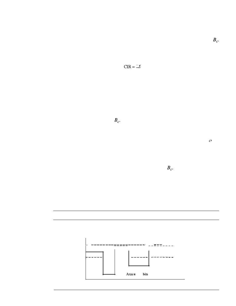
788
CHAPTER
24
CONGESTION CONTROL AND QUALITY OF SERVICE
a lower rate other times. As long as the average for the predefined period is met, the
frames will be delivered.
The cumulative number of bits sent during the predefined period cannot exceed
Note that the CIR is not an independent measurement; it can be calculated by using the
following formula:
B
bps
T
For example, if the Be is 5 kbits in a period of 5 s, the CIR is 5000/5, or 1 kbps.
Excess Burst Size
For every connection, Frame Relay defines an
excess burst size
Be"
This is the maximum
number of bits in excess of Be that a user can send during a predefined time. The network
is committed to transfer these bits if there is no congestion. Note that there is less com-
mitment here than in the case of
The network is committing itself conditionally.
User Rate
Figure 24.29 shows how a user can send bursty data.
If
the user never exceeds B
the
network is committed to transmit the frames without discarding any. If the user exceeds
Be by less than Be (that is, the total number of bits is less than Be
+
Be)' the network is
committed to transfer all the frames if there is no congestion.
If
there is congestion,
some frames will be discarded. The first switch that receives the frames from the user
has a counter and sets the DE bit for the frames that exceed
The rest of the switches
will discard these frames if there is congestion. Note that a user who needs to send data
faster may exceed the Be level. As long as the level is not above Be
+
Be' there is a
chance that the frames will reach the destination without being discarded. Remember,
however, that the moment the user exceeds the Be
+
Be level, all the frames sent after
that are discarded by the first switch.
Figure 24.29
User rate in relation to
Be and Be
+
Be
If
area is less than Be' no discarding (DE
=
0).
Rate
If area is between Be and Be
+
Be'
possible discarding if congestion (DE
=
1).
(bps)
If
area is greater than
Be
+
Be' discarding occurs.
Access rate
-
- - -
- - - -
Actual
Actual rate
Actual rate
rate
eIR
Actual rate
total
sent
in
T
s
Actual rate
T(s)
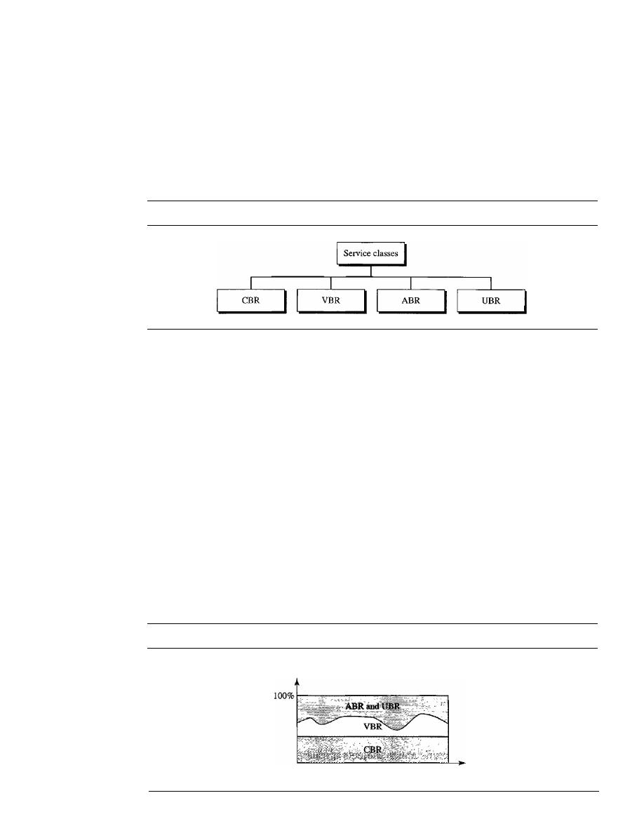
SECTION
24.9
QoS IN SWITCHED NETWORKS
789
QoSinATM
The QoS
in
ATM is based on the class, user-related attributes, and network-related attributes.
Classes
The ATM Forum defines four service classes: CBR, VBR, ABR, and UBR (see Fig-
ure 24.30).
Figure 24.30
Service classes
CBR
The
constant-bit-rate
(CBR) class is designed for customers who need real-
time audio or video services. The service is similar to that provided by a dedicated line
such as a T line.
VBR
The
variable-bit-rate
(VBR) class is divided into two subclasses: real-time
(VBR-RT) and non-real-time (VBR-NRT). VBR-RT is designed for those users who
need real-time services (such as voice and video transmission) and use compression
techniques to create a variable bit rate. VBR-NRT is designed for those users who do
not need real-time services but use compression techniques to create a variable bit rate.
ABR
The
available-bit-rate
(ABR) class delivers cells at a minimum rate.
If
more
network capacity is available, this minimum rate can be exceeded. ABR is particularly
suitable for applications that are bursty.
UBR
The
unspecified-bit-rate
(UBR) class is a best-effort delivery service that does
not guarantee anything.
Figure 24.31 shows the relationship of different classes to the total capacity of the
network.
Figure 24.31
Relationship ofservice classes to the total capacity of the network
Capacity
Time

790
CHAPTER 24
CONGESTION CONTROL AND QUAUTY OF SERVICE
User-Related Attributes
ATM defines two sets of attributes. User-related attributes are those attributes that
define how fast the user wants to send data. These are negotiated at the time of contract
between a user and a network. The following are some user-related attributes:
SCR
The
sustained cell rate
(SCR) is the average cell rate over a long time interval.
The actual cell rate may be lower or higher than this value, but the average should be
equal to or less than the SCR.
PCR
The
peak cell rate
(PCR) defines the sender's maximum cell rate. The user's
cell rate can sometimes reach this peak, as long as the SCR is maintained.
MCR
The
minimum cell rate
(MCR) defines the minimum cell rate acceptable to the
sender. For example, if the MCR is 50,000, the network must guarantee that the sender
can send at least 50,000 cells per second.
CVDT
The
cell variation delay tolerance
(CVDT) is a measure of the variation in
cell transmission times. For example, if the CVDT is 5 ns, this means that the differ-
ence between the minimum and the maximum delays in delivering the cells should not
exceed 5 ns.
N etwork-Related Attributes
The network-related attributes are those that define characteristics of the network. The
following are some network-related attributes:
CLR
The
cell loss ratio
(CLR) defines the fraction of cells lost (or delivered so late
that they are considered lost) during transmission. For example, if the sender sends
100 cells and one of them is lost, the CLR is
CLR
=
_1_
=
10-
2
100
CTD
The
cell transfer delay
(CTD) is the average time needed for a cell to travel
from source to destination. The maximum CTD and the minimum CTD are also con-
sidered attributes.
CDV
The
cell delay variation
(CDV) is the difference between the CTD maximum
and the CTD minimum.
CER
The
cell error ratio
(CER) defines the fraction of the cells delivered in error.
24.10
RECOMMENDED READING
For more details about subjects discussed in this chapter, we recommend the following
books and sites. The items in brackets [...] refer to the reference list at the end of
the text.

SECTION24.12
SUMMARY
791
Books
Congestion control and QoS are discussed in Sections 5.3 and 5.5 of [Tan03] and in
Chapter 3 of [Sta9S]. Easy reading about QoS can be found in [FH98]. The full discus-
sion of QoS is covered in [BlaOO].
24.11
KEY TERMS
access rate
additive increase
available bit rate (ABR)
average data rate
backward explicit congestion notification
(BECN)
bursty data
choke packet
closed-loop congestion control
committed burst size
Be
committed information rate (CIR)
congestion
congestion avoidance
congestion control
constant bit rate (CBR)
delay
Differentiated Services (DS or Diffserv)
effective bandwidth
excess burst size
Be
first-in, first-out (FIFO) queuing
forward explicit congestion notification
(FECN)
Integrated Services (IntServ)
jitter
leaky bucket
load
maximum burst size
multiplicative decrease
open-loop congestion control
Path message
peak data rate
per-hop behavior (PHB)
priority queuing
quality of service (QoS)
reliability
Resource Reservation Protocol (RSVP)
Resv message
slow start
throughput
token bucket
traffic shaping
unspecified bit rate (UBR)
variable bit rate (VBR)
weighted fair queuing
24.12
SUMMARY
o
The average data rate, peak data rate, maximum burst size, and effective band width
are qualitative values that describe a data flow.
o
A data flow can have a constant bit rate, a variable bit rate, or traffic that is bursty.
o
Congestion control refers to the mechanisms and techniques to control congestion
and keep the load below capacity.
o
Delay and throughput measure the performance of a network.
o
Open-loop congestion control prevents congestion; closed-loop congestion control
removes congestion.

792
CHAPTER
24
CONGESTION CONTROL AND QUALITY OF SERVICE
o
TCP avoids congestion through the use of two strategies: the combination of slow
start and additive increase, and multiplicative decrease.
D
Frame Relay avoids congestion through the use of two strategies: backward
explicit congestion notification (BECN) and forward explicit congestion notification
(FECN).
D
A flow can be characterized by its reliability, delay, jitter, and bandwidth.
o
Scheduling, traffic shaping, resource reservation, and admission control are tech-
niques to improve quality of service (QoS).
D
FIFO queuing, priority queuing, and weighted fair queuing are scheduling techniques.
o
Leaky bucket and token bucket are traffic shaping techniques.
D
Integrated Services is a flow-based QoS model designed for IP.
o
The Resource Reservation Protocol (RSVP) is a signaling protocol that helps IP
create a flow and makes a resource reservation.
o
Differential Services is a class-based QoS model designed for IP.
o
Access rate, committed burst size, committed information rate, and excess burst
size are attributes to control traffic in Frame Relay.
o
Quality of service in ATM is based on service classes, user-related attributes, and
network-related attributes.
24.13
PRACTICE SET
Review Questions
I. How are congestion control and quality of service related?
2. What is a traffic descriptor?
3. What is the relationship between the average data rate and the peak data rate?
4. What is the definition of bursty data?
5. What is the difference between open-loop congestion control and closed-loop
congestion control?
6. Name the policies that can prevent congestion.
7. Name the mechanisms that can alleviate congestion.
8. What determines the sender window size in TCP?
9. How does Frame Relay control congestion?
10. What attributes can be used to describe a flow of data?
11. What are four general techniques to improve quality of service?
12. What is traffic shaping? Name two methods to shape traffic.
13. What is the major difference between Integrated Services and Differentiated Services?
14. How is Resource Reservation Protocol related to Integrated Services?
IS. What attributes are used for traffic control in Frame Relay?
16. In regard to quality of service, how do user-related attributes differ from network-
related attributes in ATM?

SECTION 24.13
PRACTICE SET
793
Exercises
17. The address field of a Frame Relay frame is 1011000000010Ill. Is there any con-
gestion in the forward direction? Is there any congestion in the backward direction?
18. A frame goes from A to B. There is congestion in both directions. Is the PECN bit
set? Is the BECN bit set?
19. In a leaky bucket used to control liquid flow, how many gallons of liquid are left in the
bucket if the output rate is 5 gal/min, there is an input burst of 100 gal/min for 12 s,
and there is no input for 48 s?
20. An output interface in a switch is designed using the leaky bucket algorithm to
send 8000 bytes/s (tick).
If
the following frames are received in sequence, show the
frames that are sent during each second.
Frames 1, 2, 3,4:
4000 bytes each
Frames 5, 6, 7:
3200 bytes each
Frames 8, 9:
400 bytes each
Frames 10, 11, 12:
2000 bytes each
21. A user is connected to a Frame Relay network through a T-l line. The granted CIR
is 1 Mbps with a
Be of 5 million bits/5 s and Be of 1 million bits/5 s.
a. What is the access rate?
b. Can the user send data at 1.6 Mbps?
c. Can the user send data at 1 Mbps all the time? Is it guaranteed that frames are
never discarded in this case?
d. Can the user send data at 1.2 Mbps all the time? Is it guaranteed that frames are
never discarded in this case?
If
the answer is no, is it guaranteed that frames are
discarded only if there is congestion?
e. Repeat the question in part (d) for a constant rate of 1.4 Mbps.
f.
What is the maximum data rate the user can use all the time without worrying
about the frames being discarded?
g.
If
the user wants to take a risk, what is the maximum data rate that can be used
with no chance of discarding if there is no congestion?
22. In Exercise 21 the user sends data at 1.4 Mbps for 2 s and nothing for the next 3 s.
Is there a danger of discarded data if there is no congestion? Is there a danger of
discarded data if there is congestion?
23. In ATM, if each cell takes 10
to reach the destination, what is the CTD?
24. An ATM network has lost 5 cells out of 10,000 and 2 are in error. What is the CLR?
What is the CER?


Application
Layer
Objectives
The application layer enables the user, whether human or software, to access the net-
work. It provides user interfaces and support for services such as electronic mail, file
access and transfer, access to system resources, surfing the world wide web, and net-
work management.
The application layer is responsible for providing services to the user.
In this part, we briefly discuss some applications that are designed as a client/server
pair in the Internet. The client sends a request for a service to the server; the server
responds to the client.
Part 6 of the book is devoted to the application layer
and the services provided by this layer.
Chapters
This part consists of five chapters: Chapters 25 to 29.
Chapter 25
Chapter 25 discusses the Domain Name System (DNS). DNS is a client/server application
that provides name services for other applications. It enables the use of application-
layer addresses, such as an email address, instead of network layer logical addresses.
Chapter 26
Chapter 26 discusses three common applications in the Internet: remote login, electronic
mail, and file transfer. A remote login application allows the user to remotely access the
resources of a system. An electronic mail application simulates the tasks of snail mail at a
much higher speed. A file transfer application transfers files between remote systems.

Chapter 27
Chapter 27 discuss the ideas and issues in the famous world wide web (WWW).
It
also
briefly describes the client/server application program (HTTP) that is commonly used
to access the web.
Chapter 28
Chapter 28 is devoted to network management. We first discuss the general idea behind
network management. We then introduce the client/server application, SNMP, that is
used for this purpose in the Internet. Although network management can be implemented
in every layer, the Internet has decided to use a client/server application.
Chapter 29
Chapter 29 discusses multimedia and a set of wiely-used application programs. These
programs have generated new issues such as the need for new protocols in other layers
to handle the specific problems related to multimedia. We briefly discuss these issues in
this chapter.
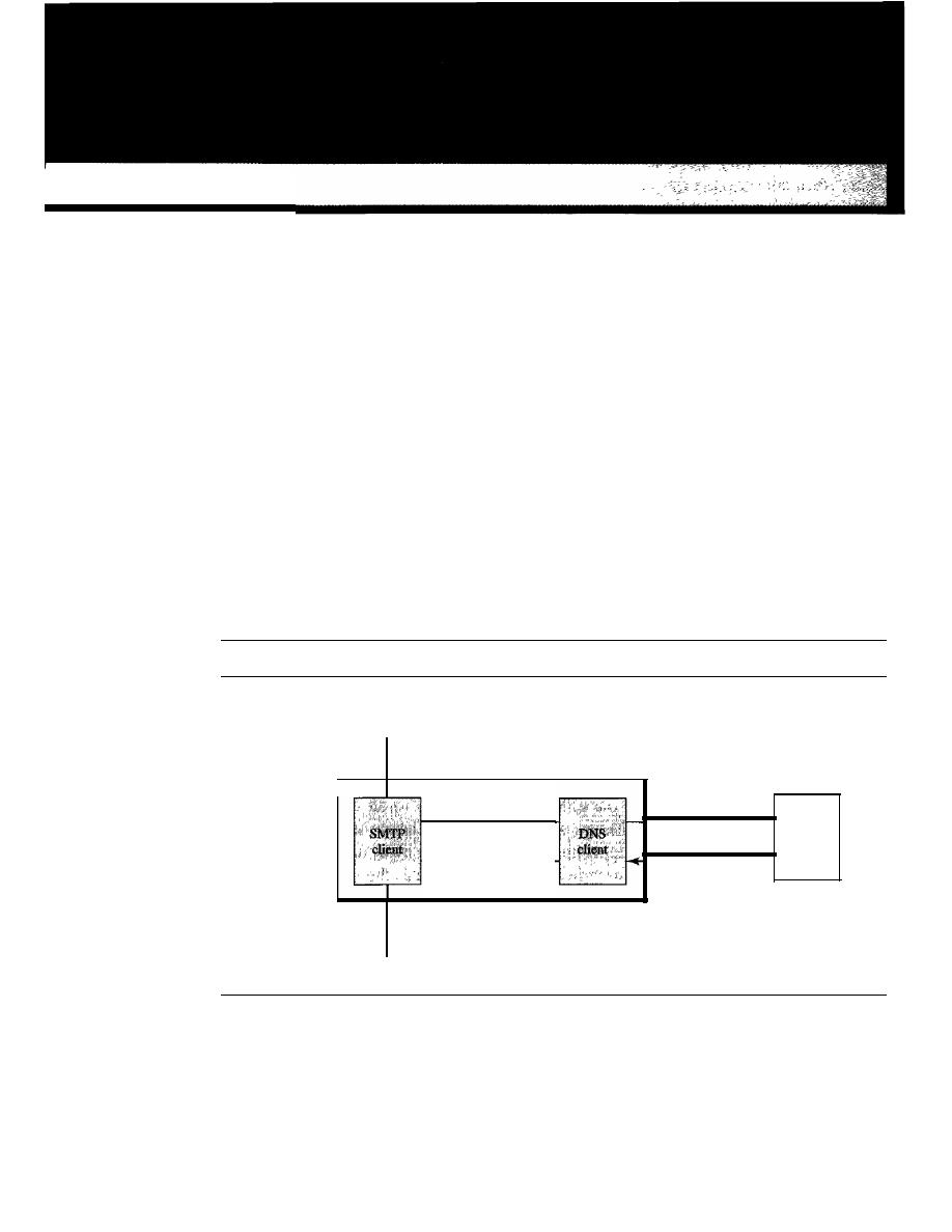
CHAPTER 25
Domain
Name
System
There are several applications in the application layer of the Internet model that follow
the client/server paradigm. The client/server programs can be divided into two categories:
those that can be directly used by the user, such as e-mail, and those that support other
application programs. The Domain Name System (DNS) is a supporting program that
is used by other programs such as e-mail.
Figure 25.1 shows an example of how a DNS client/server program can support an
e-mail program to find the IP address of an e-mail recipient. A user of an e-mail pro-
gram may know the e-mail address of the recipient; however, the IP protocol needs the
IP address. The DNS client program sends a request to a DNS server to map the e-mail
address to the corresponding IP address.
Figure 25.1
Example of using the DNS service
User
SMTP: Simple Mail Transfer Protocol (e-mail)
DNS: Domain Name System
aperson@wonderful.com
Application
layer
wonderful. com
200.200.200.5
wonderfuI.com
200.200.200.5
DNS
client
200.200.200.5
Transport layer
To identify an entity, TCPIIP protocols use the IP address, which uniquely identi-
fies the connection of a host to the Internet. However, people prefer to use names
instead of numeric addresses. Therefore, we need a system that can map a name to an
address or an address to a name.
797

798
CHAPTER
25
DOMAIN NAME SYSTEM
When the Internet was small, mapping was done by using a
host file. The host file
had only two columns: name and address. Every host could store the host file on its
disk and update it periodically from a master host file. When a program or a user
wanted to map a name to an address, the host consulted the host file and found the
mapping.
Today, however, it is impossible to have one single host file to relate every address
with a name and vice versa. The host file would be too large to store in every host. In
addition, it would be impossible to update all the host files every time there was a
change.
One solution would be to store the entire host file in a single computer and allow
access to this centralized information to every computer that needs mapping. But we
know that this would create a huge amount of traffic on the Internet.
Another solution, the one used today, is to divide this huge amount of information
into smaller parts and store each part on a different computer. In this method, the host
that needs mapping can contact the closest computer holding the needed information.
This method is used by the
Domain Name System (DNS). In this chapter, we first
discuss the concepts and ideas behind the DNS. We then describe the DNS protocol
itself.
25.1
NAME SPACE
To be unambiguous, the names assigned to machines must be carefully selected from a
name space with complete control over the binding between the names and IP addresses.
In other words, the names must be unique because the addresses are unique. A
name
space that maps each address to a unique name can be organized in two ways: fiat or
hierarchical.
Flat Narne Space
In a
flat name space, a name is assigned to an address. A name in this space is a
sequence of characters without structure. The names mayor may not have a common
section; if they do, it has no meaning. The main disadvantage of a fiat name space is
that it cannot be used in a large system such as the Internet because it must be centrally
controlled to avoid ambiguity and duplication.
Hierarchical Narne Space
In a
hierarchical name space, each name is made of several parts. The first part can
define the nature of the organization, the second part can define the name of an organiza-
tion, the third part can define departments in the organization, and so on. In this case, the
authority to assign and control the name spaces can be decentralized. A central authority
can assign the part of the name that defines the nature of the organization and the name
of the organization. The responsibility of the rest of the name can be given to the organi-
zation itself. The organization can add suffixes (or prefixes) to the name to define its host
or resources. The management of the organization need not worry that the prefix chosen
for a host is taken by another organization because, even if part of an address is the
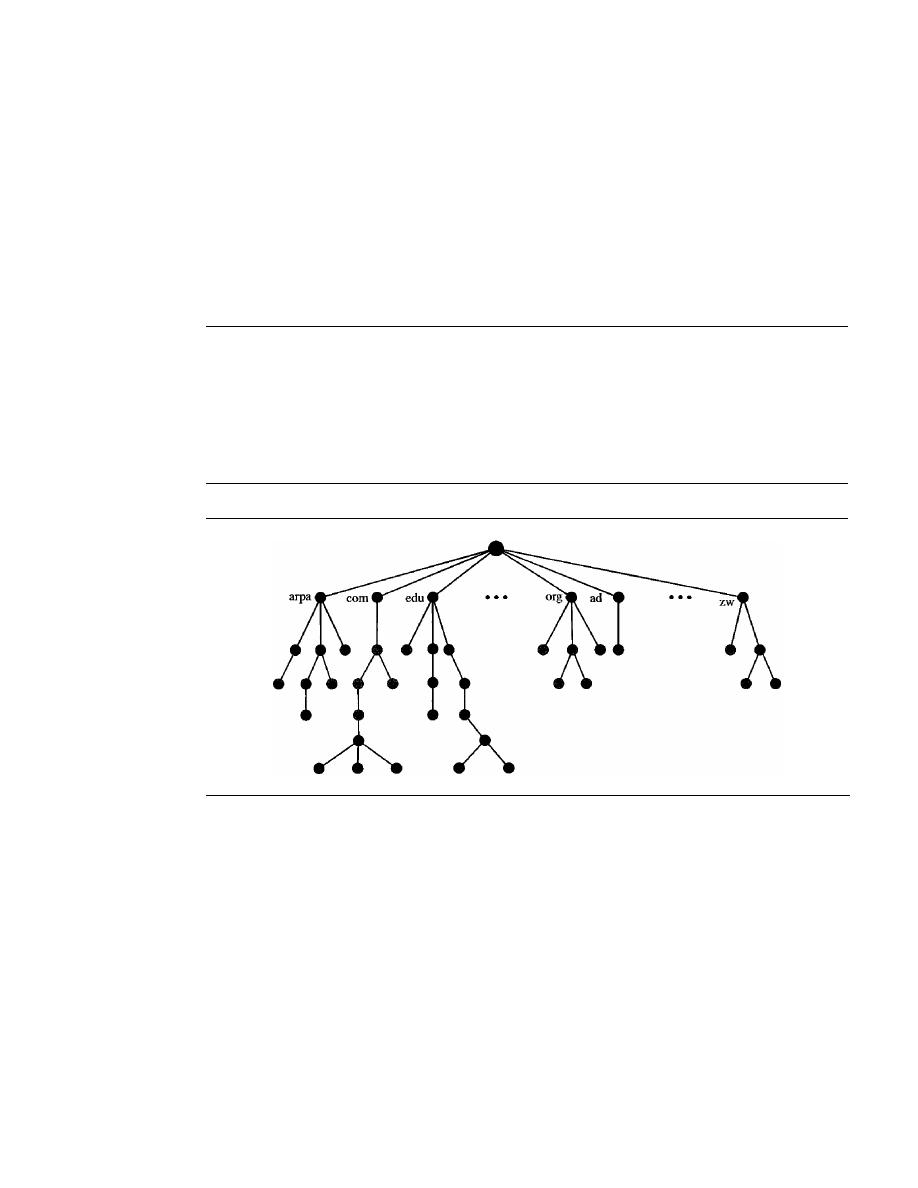
SECTION
25.2
DOMAIN NAME SPACE
799
same, the whole address is different. For example, assume two colleges and a company
call one of their computers
challenger.
The first college is given a name by the central
authority such as
jhda.edu,
the second college is given the name
berkeley.edu,
and the
company is given the name
smart. com.
When these organizations add the name
chal-
lenger
to the name they have already been given, the end result is three distinguishable
names:
challenger.jhda.edu, challenger.berkeley.edu,
and
challenger.smart.com.
The names
are unique without the need for assignment by a central authority. The central authority
controls only part of the name, not the whole.
25.2
DOMAIN NAME SPACE
To have a hierarchical name space, a
domain name space
was designed. In this design
the names are defined in an inverted-tree structure with the root at the top. The tree can
have only 128 levels: level 0 (root) to level 127 (see Figure 25.2).
Figure 25.2
Domain name space
Label
Each node in the tree has a
label,
which is a string with a maximum of 63 characters.
The root label is a null string (empty string). DNS requires that children of a node
(nodes that branch from the same node) have different labels, which guarantees the
uniqueness of the domain names.
Domain Name
Each node in the tree has a domain name. A full
domain name
is a sequence of labels
separated by dots (.). The domain names are always read from the node up to the root.
The last label is the label of the root (null). This means that a full domain name always
ends in a null label, which means the last character is a dot because the null string is
nothing. Figure 25.3 shows some domain names.
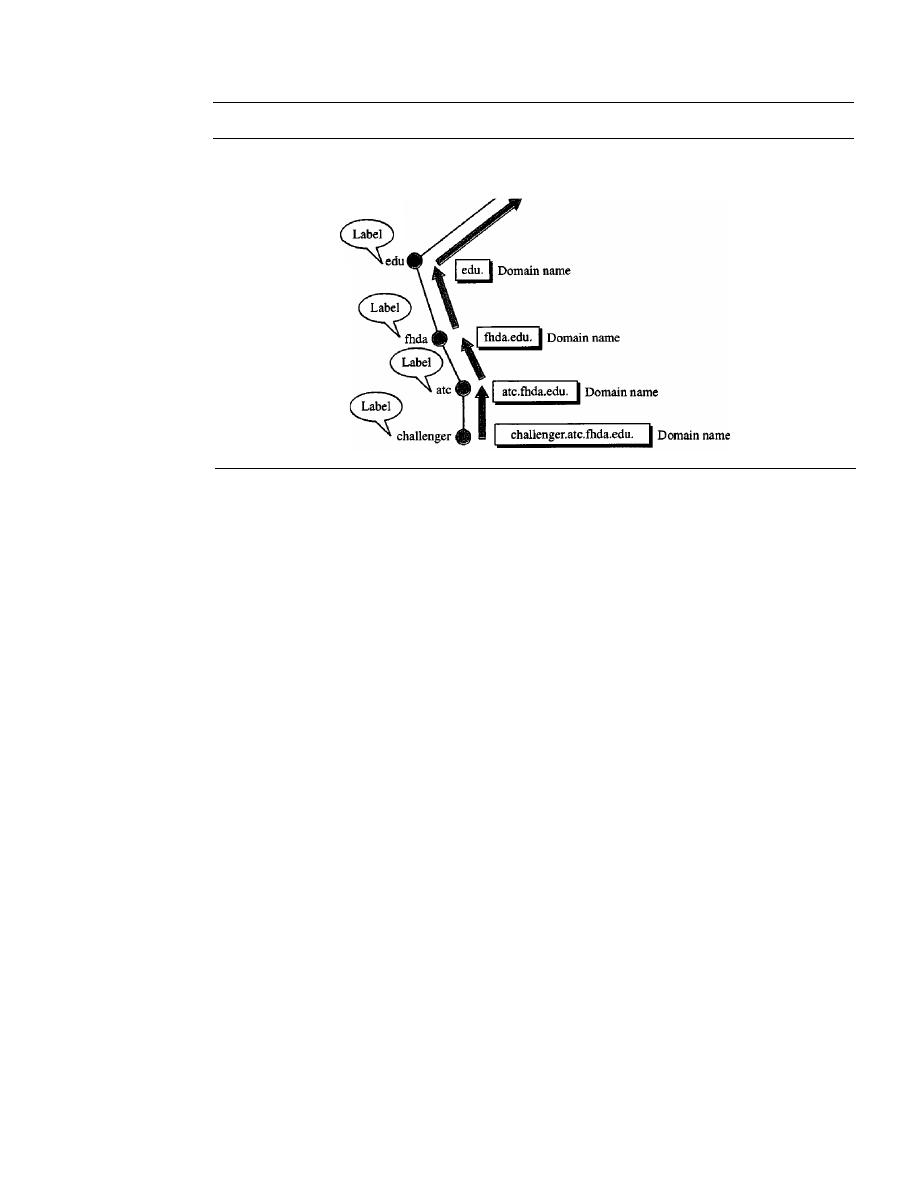
800
CHAPTER
25
DOMAIN NAME SYSTEM
Figure 25.3
Domain names and labels
Root
Fully Qualified Domain Name
If
a label is terminated by a null string,
it
is called a fully qualified domain name
(FQDN). An FQDN is a domain name that contains the full name of a host. It contains
all labels, from the most specific to the most general, that uniquely define the name of
the host. For example, the domain name
challenger.ate.tbda.edu.
is the FQDN of a computer named
challenger
installed at the Advanced Technology
Center (ATC) at De Anza College. A DNS server can only match an FQDN to an
address. Note that the name must end with a null label, but because null means nothing,
the label ends with a dot (.).
Partially Qualified Domain Name
If
a label is not terminated by a null string, it is called a partially qualified domain
name (PQDN). A PQDN starts from a node, but it does not reach the root. It is used
when the name to be resolved belongs to the same site as the client. Here the resolver
can supply the missing part, called the
suffix,
to
create an FQDN. For example, if a user
at the jhda.edu. site wants to get the IP address of the challenger computer, he or she
can define the partial name
challenger
The DNS client adds the suffix atc.jhda.edu. before passing the address to the DNS
server.
The DNS client normally holds a list of suffixes. The following can be the list of
suffixes at De Anza College. The null suffix defines nothing. This suffix is added when
the user defines an FQDN.
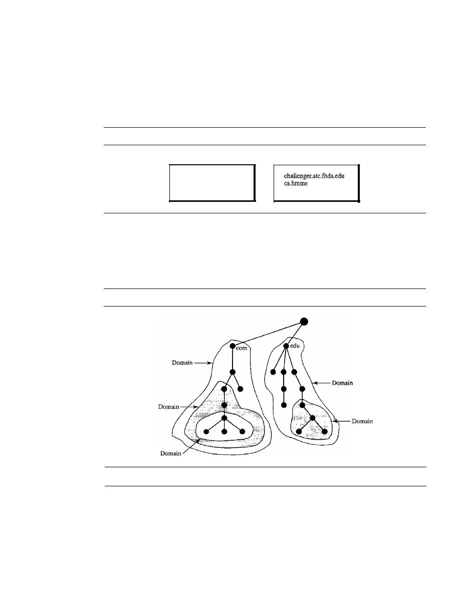
SECTION
25.3
DISTRIBUTION OF NAME SPACE
801
atc.fhda.edu
fhda.edu
null
Figure 25.4 shows some FQDNs and PQDNs.
Figure 25.4
FQDN and PQDN
FQDN
challenger.atc.fhda.edu.
cs.hnune.com.
www.funny.int.
Domain
PQDN
www
A domain is a subtree of the domain name space. The name of the domain is the domain
name of the node at the top of the subtree. Figure 25.5 shows some domains. Note that a
domain may itself be divided into domains (or subdomains as they are sometimes called).
Figure 25.5
Domains
25.3
DISTRIBUTION OF NAME SPACE
The information contained in the domain name space must be stored. However, it is
very inefficient and also unreliable to have just one computer store such a huge amount
of information. It is inefficient because responding to requests from all over the world
places a heavy load on the system. It is not unreliable because any failure makes the data
inaccessible.
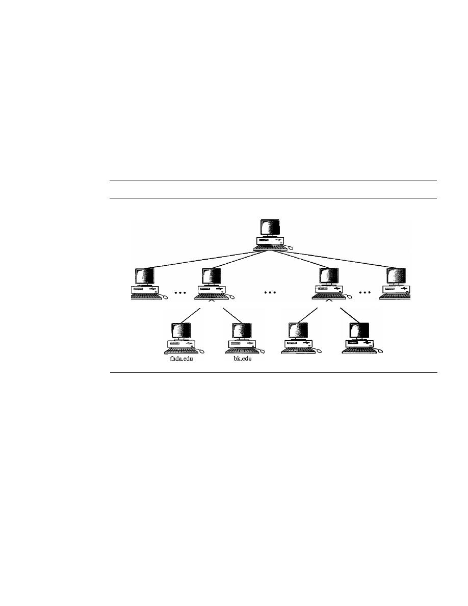
802
CHAPTER
25
DOMAIN NAME SYSTEM
Hierarchy of Name Servers
The solution to these problems is to distribute the information among many computers
called DNS servers. One way to do this is to divide the whole space into many domains
based on the first level. In other words, we let the root stand alone and create as many
domains (subtrees) as there are first-level nodes. Because a domain created in this way
could be very large, DNS allows domains to be divided further into smaller domains
(subdomains). Each server can be responsible (authoritative) for either a large or a
small domain. In other words, we have a hierarchy of servers in the same way that we
have a hierarchy of names (see Figure 25.6).
Figure 25.6
Hierarchy of name servers
Root server
irwin.com
com server
us server
...
.
mcgraw.com
edu server
arpa server
Zone
Since the complete domain name hierarchy cannot be stored on a single server, it is
divided among many servers. What a server is responsible for or has authority over is
called a zone. We can define a zone as a contiguous part of the entire tree. If a server
accepts responsibility for a domain and does not divide the domain into smaller
domains, the domain and the zone refer to the same thing. The server makes a database
called a zone file and keeps all the information for every node under that domain. How-
ever, if a server divides its domain into subdomains and delegates part of its authority to
other servers, domain and zone refer to different things. The information about the
nodes in the subdomains is stored in the servers at the lower levels, with the original
server keeping some sort of reference to these lower-level servers. Of course the origi-
nal server does not free itself from responsibility totally: It still has a zone, but the
detailed information is kept by the lower-level servers (see Figure 25.7).
A server can also divide part of its domain and delegate responsibility but still keep
part of the domain for itself. In this case, its zone is made of detailed information for the
part of the domain that is not delegated and references to those parts that are delegated.
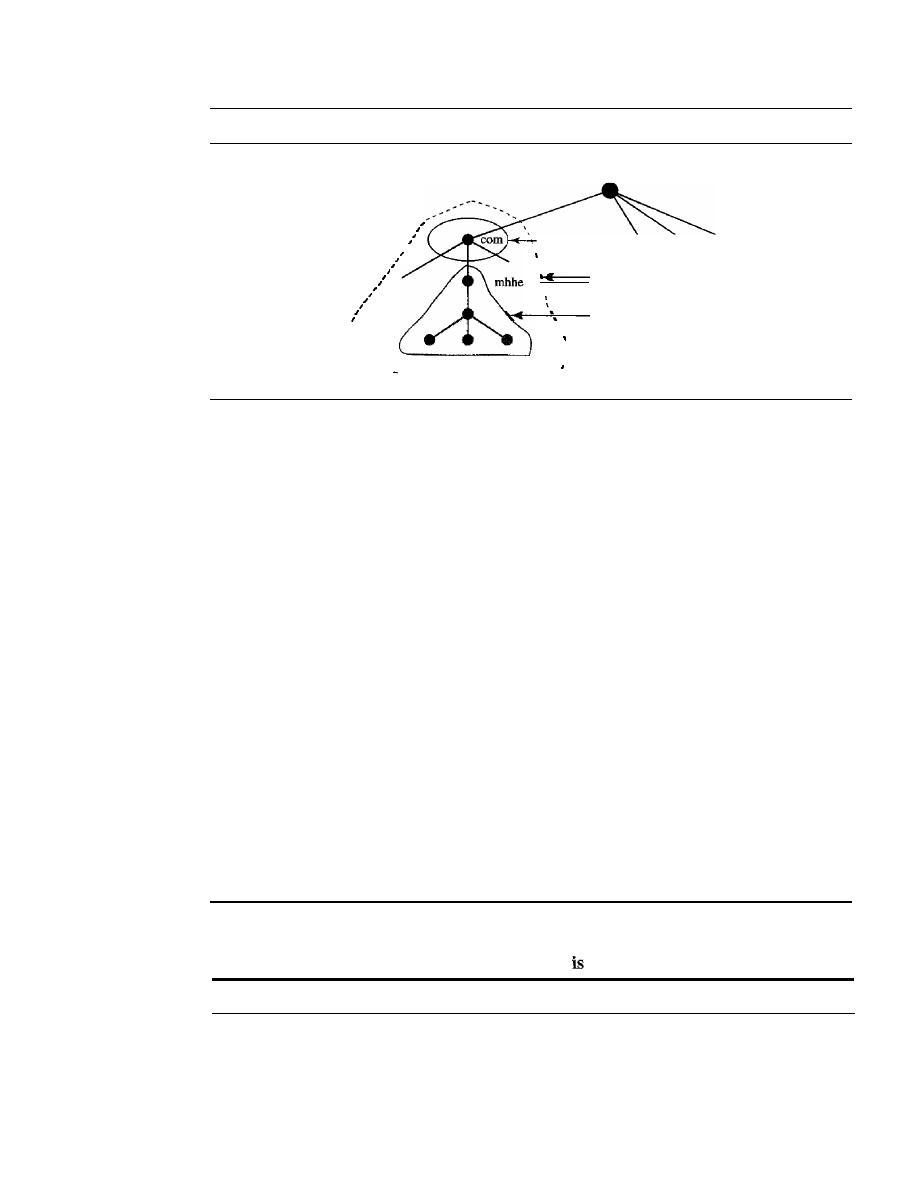
SECTION
25.4
DNS IN THE INTERNET
803
Figure 25.7
Zones and domains
Root
I
I
,
I
,
, - - - Zone
,
.
,
Domain
I
Zone and
domain
.
I
1
,
--
_---- --
..
_--------
Root Server
A root server
is a server whose zone consists of the whole tree.
A
root server usually
does not store any information about domains but delegates its authority to other servers,
keeping references to those servers. There are several root servers, each covering the
whole domain name space. The servers are distributed all around the world.
Primary and Secondary Servers
DNS defines two types of servers: primary and secondary.
A primary server
is a server
that stores a file about the zone for which it is an authority.
It
is responsible for creating,
maintaining, and updating the zone file.
It
stores the zone file on a local disk.
A secondary server
is a server that transfers the complete information about a
zone from another server (primary or secondary) and stores the file on its local disk. The
secondary server neither creates nor updates the zone files.
If
updaJing is required, it
must be done by the primary server, which sends the updated version to the secondary.
The primary and secondary servers are both authoritative for the zones they serve.
The idea is not to put the secondary server at a lower level of authority but to create
redundancy for the data so that if one server fails, the other can continue serving clients.
Note also that a server can be a primary server for a specific zone and a secondary server
for another zone. Therefore, when we refer to a server as a primary or secondary server,
we should be careful to which zone we refer.
A primary server loads all information from the disk file; the secondary server
loads all information from the primary server. When the secondary downloads
information from the primary, it
called zone transfer.
25.4
DNS IN THE INTERNET
DNS is a protocol that can be used in different platforms. In the Internet, the domain
name space (tree) is divided into three different sections: generic domains, country
domains, and the inverse domain (see Figure 25.8).
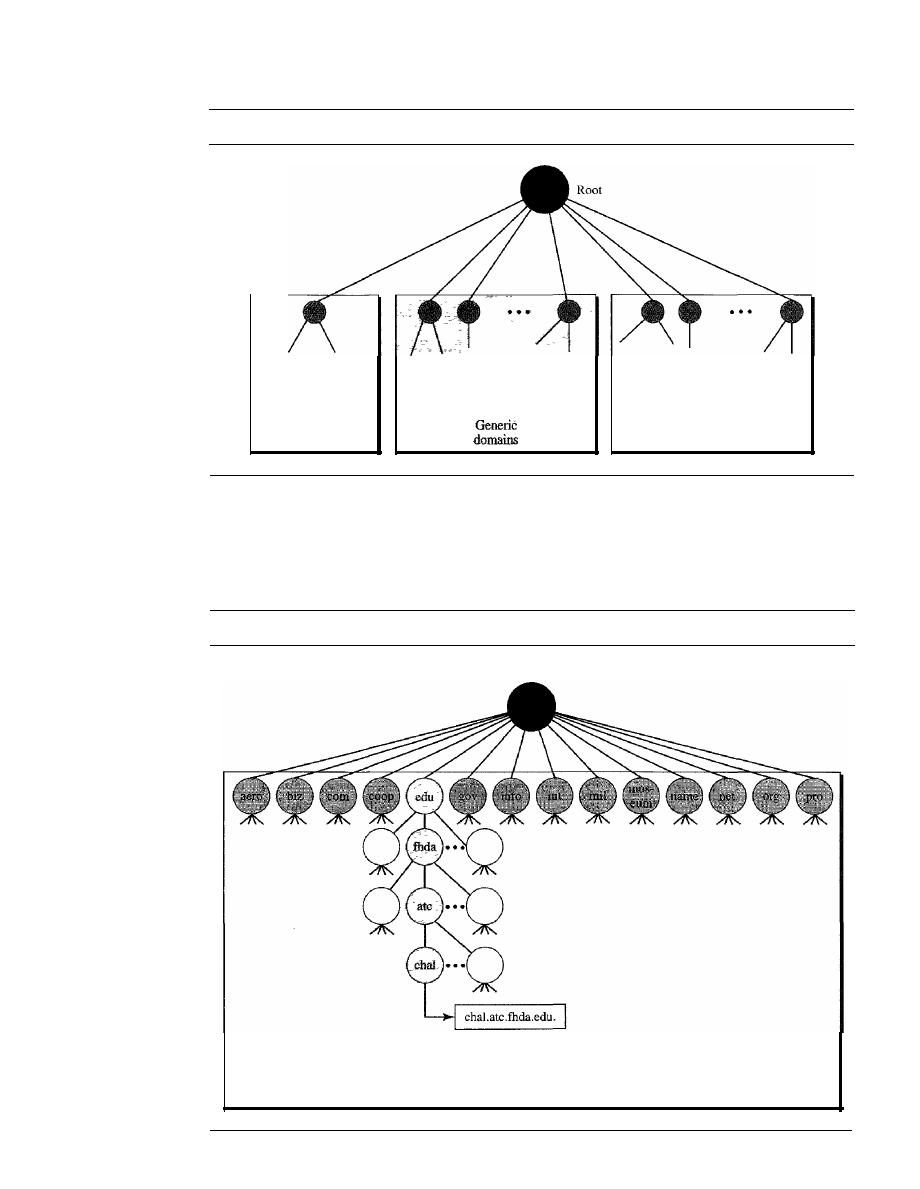
804
CHAPTER
25
DOMAIN NAME SYSTEM
Figure 25.8
DNS used in the Internet
Inverse
domain
Generic Domains
Country
domains
The
generic domains define registered hosts according to their generic behavior. Each
node in the tree defines a domain, which is an index to the domain name space database
(see Figure 25.9).
Figure 25.9
Generic domains
Root level
Index to addresses
Generic domains

SECTION
25.4
DNS IN THE INTERNET
805
Looking at the tree, we see that the first level in the generic domains section allows
14 possible labels. These labels describe the organization types as listed in Table 25.1.
Table 25.1
Generic domain labels
Label
Description
aero
Airlines and aerospace companies
biz
Businesses or firms (similar to "com")
com
Commercial organizations
coop
Cooperative business organizations
edu
Educational institutions
gov
Government institutions
info
Information service providers
int
International organizations
mil
Military groups
museum
Museums and other nonprofit organizations
name
Personal names (individuals)
net
Network support centers
org
Nonprofit organizations
pro
Professional individual organizations
Country Domains
The
country domains
section uses two-character country abbreviations (e.g., us for
United States). Second labels can be organizational, or they can be more specific,
national designations. The United States, for example, uses state abbreviations as a
subdivision of us (e.g., ca.us.).
Figure 25.10 shows the country domains section. The address
anza.cup.ca.us
can
be translated to De Anza College in Cupertino, California, in the United States.
Inverse Domain
The
inverse domain
is used to map an address to a name. This may happen, for exam-
ple, when a server has received a request from a client to do a task. Although the server
has a file that contains a list of authorized clients, only the IP address of the client
(extracted from the received IP packet) is listed. The server asks its resolver to send a
query to the DNS server to map an address to a name to determine if the client is on the
authorized list.
This type of query is called an inverse or pointer (PTR) query. To handle a pointer
query, the inverse domain is added to the domain name space with the first-level node
called
arpa
(for historical reasons). The second level is also one single node named
in-addr
(for inverse address). The rest of the domain defines IP addresses.
The servers that handle the inverse domain are also hierarchical. This means the netid
part of the address should be at a higher level than the subnetid part, and the subnetid part
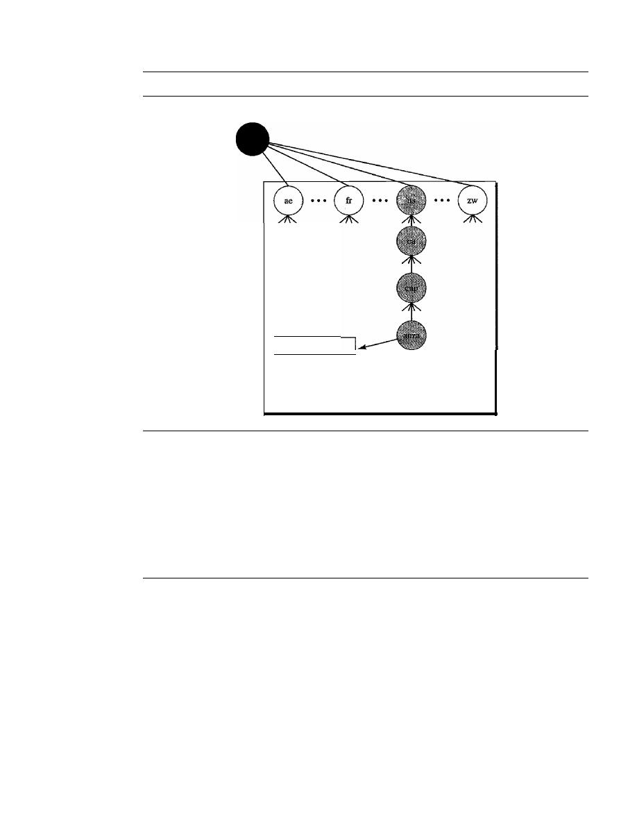
806
CHAPTER
25
DOMAIN NAME SYSTEM
Figure 25.10
Country domains
Root level
anza.cup.ca.us.
Index to addresses
Country domains
higher than the hostid part. In this way, a server serving the whole site is at a higher level
than the servers serving each subnet. This configuration makes the domain look inverted
when compared to a generic or country domain. To follow the convention of reading the
domain labels from the bottom to the top, an IF address such as 132.34.45.121 (a class B
address with netid 132.34) is read as 121.45.34.132.in-addr. arpa. See Figure 25.11 for an
illustration of the inverse domain configuration.
25.5
RESOLUTION
Mapping a name to an address or an address to a name is called name-address resolution.
Resolver
DNS is designed as a client/server application. A host that needs to map an address to a
name or a name to an address calls a DNS client called a resolver. The resolver accesses
the closest DNS server with a mapping request. If the server has the information, it
satisfies the resolver; otherwise, it either refers the resolver to other servers or asks other
servers to provide the infonnation.
After the resolver receives the mapping, it interprets the response to see if it is a
real resolution or an error, and finally delivers the result to the process that requested it.
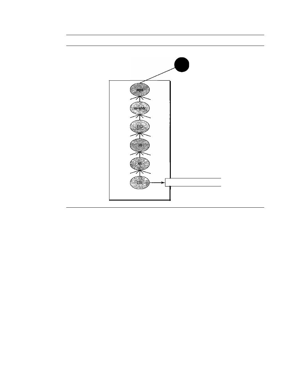
SECTION
25.5
RESOLUTION
807
Figure 25.11
Inverse domain
Root level
l21.45.34.132.in-addr.arpa.
Index to names
Inverse domain
Mapping Names to Addresses
Most of the time, the resolver gives a domain name to the server and asks for the corre-
sponding address.
In
this case, the server checks the generic domains or the country
domains to find the mapping.
If
the domain name is from the generic domains section, the resolver receives a
domain name such as "chal.atc.jhda.edu.". The query is sent by the resolver to the local
DNS server for resolution.
If
the local server cannot resolve the query,
it
either refers
the resolver to other servers or asks other servers directly.
If
the domain name is from the country domains section, the resolver receives a
domain name such as "ch.jhda.cu.ca.us.". The procedure is the same.
Mapping Addresses to Names
A client can send an
IP
address to a server to be mapped to a domain name. As mentioned
before, this is called a PTR query. To answer queries of this kind, DNS uses the inverse
domain. However, in the request, the
IP
address is reversed and the two labels in-addr and
arpa
are appended to create a domain acceptable by the inverse domain section. For
example, if the resolver receives the IF address 132.34.45.121, the resolver first inverts
the address and then adds the two labels before sending. The domain name sent is
"121.45.34.132.in-addr.arpa."
which is received by the local DNS and resolved.
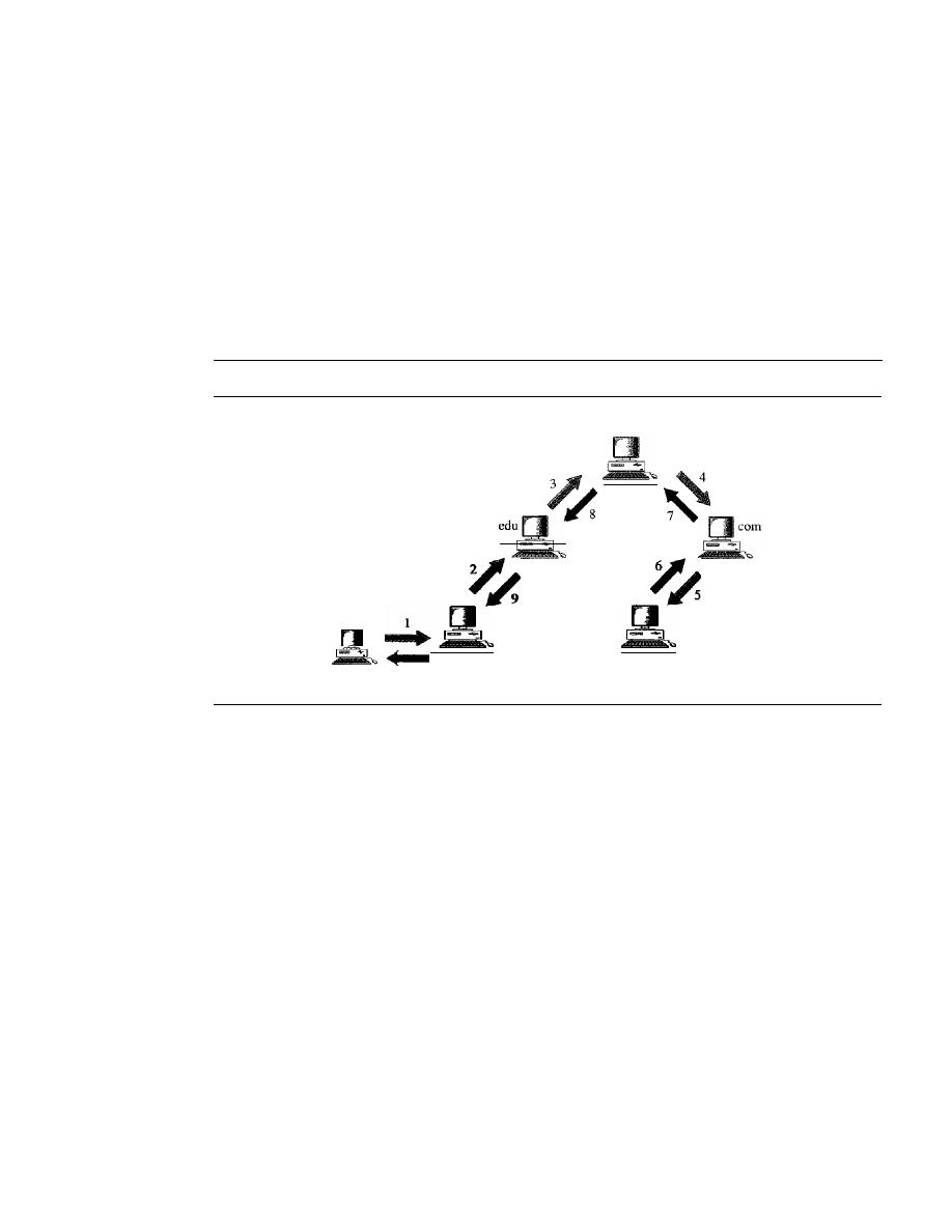
808
CHAPTER
25
DOMAIN NAME SYSTEM
Recursive Resolution
The client (resolver) can ask for a recursive answer from a name server. This means that
the resolver expects the server to supply the final answer.
If
the server is the authority
for the domain name, it checks its database and responds.
If
the server is not the author-
ity, it sends the request to another server (the parent usually) and waits for the response.
If the parent is the authority, it responds; otherwise, it sends the query to yet another
server. When the query is finally resolved, the response travels back until it finally
reaches the requesting client. This is called recursive resolution and is shown in
Figure 25.12.
Figure 25.12
Recursive resolution
Root server
...
fhda.edu
mcgraw.com
Client
10
Iterative Resolution
If the client does not ask for a recursive answer, the mapping can be done iteratively. If
the server is an authority for the name, it sends the answer. If it is not, it returns (to the
client) the IP address of the server that it thinks can resolve the query. The client is
responsible for repeating the query to this second server. If the newly addressed server
can resolve the problem, it answers the query with the IP address; otherwise, it returns
the IP address of a new server to the client. Now the client must repeat the query to the
third server. This process is called iterative resolution because the client repeats the
same query to multiple servers. In Figure 25.13 the client queries four servers before it
gets an answer from the mcgraw.com server.
Caching
Each time a server receives a query for a name that is not in its domain, it needs to
search its database for a server IP address. Reduction of this search time would increase
efficiency. DNS handles this with a mechanism called caching. When a server asks for
a mapping from another server and receives the response, it stores this information in
its cache memory before sending it to the client.
If
the same or another client asks for
the same mapping, it can check its cache memory and solve the problem. However, to
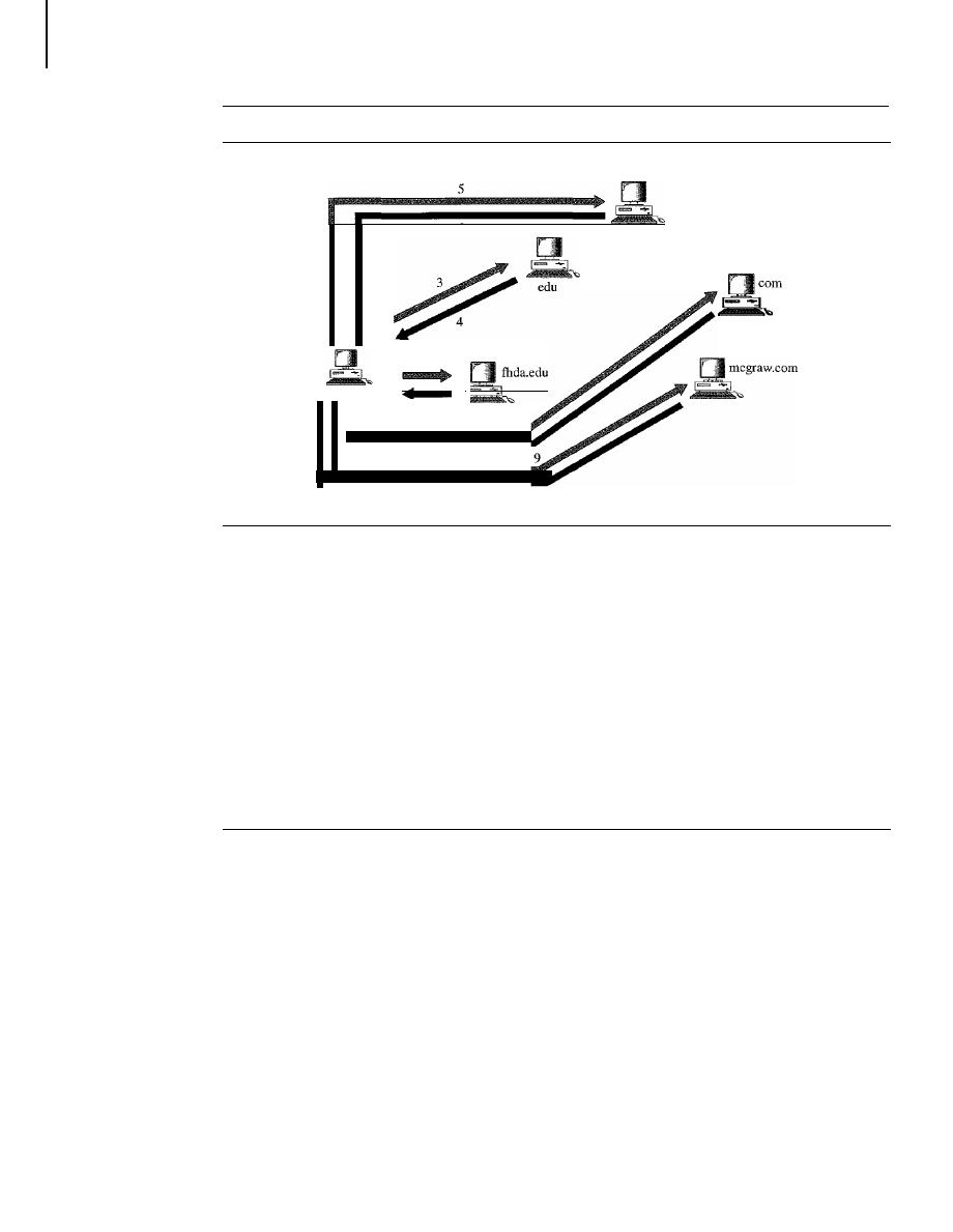
SECTION
25.6
DNS MESSAGES
809
Figure 25.13
Iterative resolution
Root server
6
Client
I
2
7
8
10
inform the client that the response is coming from the cache memory and not from an
authoritative source, the server marks the response as unauthoritative.
Caching speeds up resolution, but it can also be problematic.
If
a server caches a
mapping for a long time, it may send an outdated mapping to the client. To counter this,
two techniques are used. First, the authoritative server always adds information to the
mapping called time-to-live (TTL). It defines the time in seconds that the receiving
server can cache the information. After that time, the mapping is invalid and any query
must be sent again to the authoritative server. Second, DNS requires that each server
keep a TTL counter for each mapping it caches. The cache memory must be searched
periodically, and those mappings with an expired TTL must be purged.
25.6
DNS MESSAGES
DNS has two types of messages: query and response. Both types have the same format.
The query message consists of a header and question records; the response message
consists of a header, question records, answer records, authoritative records, and addi-
tional records (see Figure 25.14).
Header
Both query and response messages have the same header format with some fields set
to zero for the query messages. The header is 12 bytes, and its format is shown in
Figure 25.15.
The identification subfield is used by the client to match the response with the query.
The client uses a different identification number each time it sends a query. The server
duplicates this number in the corresponding response. The
flags
subfield is a collection of
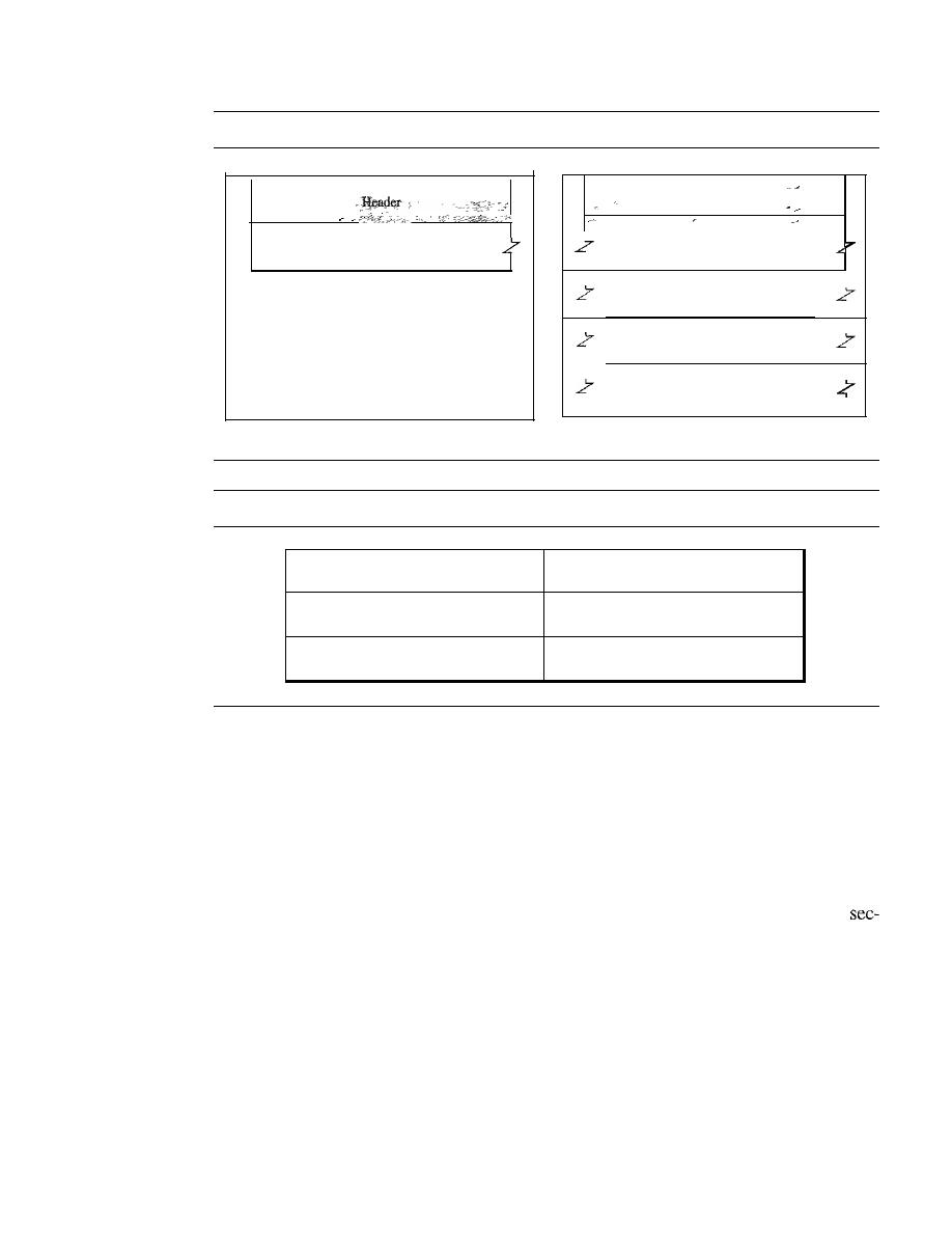
810
CHAPTER
25
DOMAIN NAME SYSTEM
Figure 25.14
Query and response messages
Question section
a. Query
Figure 25.15
Header format
.-
Header
Question section
Answer section
Authoritative section
Additional section
b. Response
Identification
Flags
Number of question records
Number of answer records
(all Os in query message)
Number of authoritative records
Number of additional records
(all Os in query message)
(all Os in query message)
subfields that define the type of the message, the type of answer requested, the type of
desired resolution (recursive or iterative), and so on. The number ofquestion records sub-
field contains the number of queries in the question section of the message. The number
of answer records
subfield contains the number of answer records in the answer section
of the response message. Its value is zero in the query message. The number ofauthorita-
tive records
subfield contains the number of authoritative records in the authoritative sec-
tion of a response message. Its value is zero in the query message. Finally, the number of
additional records
subfield contains the number additional records in the additional
tion of a response message. Its value is zero in the query message.
Question Section
This is a section consisting of one or more question records. It is present on both query
and response messages. We will discuss the question records in a following section.
Answer Section
This is a section consisting of one or more resource records. It is present only on response
messages. This section includes the answer from the server to the client (resolver). We
will discuss resource records in a following section.

SECTION
25.8
REGISTRARS
811
Authoritative Section
This is a section consisting of one or more resource records.
It
is present only on response
messages. This section gives infonnation (domain name) about one or more authoritative
servers for the query.
Additional Information Section
This is a section consisting of one or more resource records.
It
is present only on response
messages. This section provides additional infonnation that may help the resolver. For
example, a server may give the domain name of an authoritative server to the resolver in
the authoritative section, and include the IP address of the same authoritative server in the
additional information section.
25.7
TYPES OF RECORDS
As we saw in Section 25.6, two types of records are used in DNS. The question records
are used in the question section of the query and response messages. The resource
records are used in the answer, authoritative, and additional information sections of the
response message.
Question Record
A
question record
is used by the client to get information from a server. This contains
the domain name.
- Resource Record
Each domain name (each node on the tree) is associated with a record called the
resource
record.
The server database consists of resource records. Resource records are also what
is returned by the server to the client.
25.8
REGISTRARS
How are new domains added to
DNS?
This is done through a
registrar,
a commercial
entity accredited by
ICANN. A registrar first verifies that the requested domain name is
unique and then enters it into the
DNS
database. A fee is charged.
Today, there are many registrars; their names and addresses can be found at
http://www.intenic.net
To register, the organization needs to give the name of its server and the IP address
of the server. For example, a new commercial organization named
wonderful with a
server named
ws and IP address 200.200.200.5 needs to give the following information
to one of the registrars:
Domain name:
WS.
wonderful.com
IP
address:
200.200.200.5

812
CHAPTER
25
DOMAIN NAME SYSTEM
25.9
DYNAMIC DOMAIN NAME SYSTEM (DDNS)
When the DNS was designed, no one predicted that there would be so many address
changes. In DNS, when there is a change, such as adding a new host, removing a host,
or changing an IP address, the change must be made to the DNS master file. These types
of changes involve a lot of manual updating. The size of today's Internet does not allow
for this kind of manual operation.
The DNS master file must be updated dynamically. The Dynamic Domain Name
System (DDNS) therefore was devised to respond to this need. In DDNS, when a bind-
ing between a name and an address is determined, the information is sent, usually by
DHCP (see Chapter 21) to a primary DNS server. The primary server updates the zone.
The secondary servers are notified either actively or passively. In active notification, the
primary server sends a message to the secondary servers about the change in the zone,
whereas in passive notification, the secondary servers periodically check for any changes.
In either case, after being notified about the change, the secondary requests information
about the entire zone (zone transfer).
To provide security and prevent unauthorized changes in the DNS records, DDNS
can use an authentication mechanism.
25.10
ENCAPSULATION
DNS can use either UDP or TCP. In both cases the
port used by the server
is port 53. UDP is used when the size of the response message is less than 512 bytes
because most UDP packages have a 512-byte packet size limit.
If
the size of the
response message is more than 512 bytes, a TCP connection is used. In that case, one of
two scenarios can occur:
o
If the resolver has prior knowledge that the size of the response message is more
than 512 bytes, it uses the TCP connection. For example, if a secondary name
server (acting as a client) needs a zone transfer from a primary server, it uses the
TCP connection because the size of the information being transferred usually
exceeds 512 bytes.
o
If the resolver does not know the size of the response message, it can use the UDP
port. However, if the size of the response message is more than 512 bytes, the
server truncates the message and turns on the TC bit. The resolver now opens a
TCP connection and repeats the request to get a full response from the server.
DNS can use the services of UDP or TCP using the well-known port 53.
25.11
RECOMMENDED READING
For more details about subjects discussed in this chapter, we recommend the following
books and sites. The items in brackets [...] refer to the reference list at the end of the text.
SECTION
25.13
SUMMARY
813
Books
DNS is discussed
in
[AL98], Chapter 17 of [For06], Section 9.1 of [PD03], and Section 7.1
of [Tan03].
Sites
The following sites are related to topics discussed in this chapter.
o
www.intenic.net/Information about registrars
D
www.ietf.org/rfc.html
Information about RFCs
RFCs
The following RFCs are related to DNS:
1034,1035,1386,1480,1535,1536,1537,
25.12
KEY TERMS
caching
country domain
DNS server
domain
domain name
domain name space
Domain Name System (DNS)
Dynamic Domain Name System (DDNS)
flat name space
fully qualified domain name (FQDN)
generic domain
hierarchical name space
host file
inverse domain
iterative resolution
label
name space
partially qualified domain name (PQDN)
primary server
query message
question record
recursive resolution
registrar
resolver
resource record
response message
root server
secondary server
subdomain
suffix
zone
25.13
SUMMARY
o
The Domain Name System (DNS) is a client/server application that identifies each
host on the Internet with a unique user-friendly name.
D
DNS organizes the name space in a hierarchical structure to decentralize the
responsibilities involved in naming.

814
CHAPTER
25
DOMAIN NAME SYSTEM
D
DNS can be pictured as an inverted hierarchical tree structure with one root node at
the top and a maximum of 128 levels.
D
Each node in the tree has a domain name.
D
A domain is defined as any subtree of the domain name space.
D
The name space information is distributed among DNS servers. Each server has
jurisdiction over its zone.
D
A root server's zone is the entire DNS tree.
D
A primary server creates, maintains, and updates information about its zone.
D
A secondary server gets its information from a primary server.
D
The domain name space is divided into three sections: generic domains, country
domains, and inverse domain.
D
There are 14 generic domains, each specifying an organization type.
D
Each country domain specifies a country.
D
The inverse domain finds a domain name for a given IP address. This is called
address-to-name resolution.
D
Name servers, computers that run the DNS server program, are organized in a
hierarchy.
D
The DNS client, called a resolver, maps a name to an address or an address to a name.
D
In recursive resolution, the client sends its request to a server that eventually
returns a response.
D
In iterative resolution, the client may send its request to multiple servers before
getting an answer.
D
Caching is a method whereby an answer to a query is stored in memory (for a limited
time) for easy access to future requests.
D
A fully qualified domain name (FQDN) is a domain name consisting of labels begin-
ning with the host and going back through each level to the root node.
D
A partially qualified domain name (PQDN) is a domain name that does not include
all the levels between the host and the root node.
D
There are two types of DNS messages: queries and responses.
D
There are two types of DNS records: question records and resource records.
D
Dynamic DNS (DDNS) automatically updates the DNS master file.
D
DNS uses the services ofUDP for messages of less than 512 bytes; otherwise, TCP
is used.
25.14
PRACTICE SET
Review Questions
I. What is an advantage of a hierarchical name space over a flat name space for a system
the size of the Internet?
2. What is the difference between a primary server and a secondary server?
3. What are the three domains of the domain name space?

SECTION 25.14
PRACTICE SET
815
4. What is the purpose of the inverse domain?
5. How does recursive resolution differ from iterative resolution?
6. What is an FQDN?
7. What is a PQDN?
8. What is a zone?
9. How does caching increase the efficiency of name resolution?
10. What are the two main categories ofDNS messages?
11. Why was there a need for DDNS?
Exercises
12. Determine which of the following is an FQDN and which is a PQDN.
a. xxx
b. xxx.yyy.
c. xxx.yyy.net
d. zzz.yyy.xxx.edu.
13. Determine which of the following is an FQDN and which is a PQDN.
a.
mil.
b. edu.
c. xxx.yyy.net
d. zzz. yyy.xxx.edu
14. Which domain is used by your system, generic or country?
15. Why do we need a DNS system when we can directly use an IP address?
16. To find the IP address of a destination, we need the service of DNS. DNS needs the
service of UDP or TCP. UDP or TCP needs the service of IP. IP needs an IP desti-
nation address. Is this a vicious cycle here?
17.
If
a DNS domain name is
voyager.fhda.edu,
how many labels are involved here?
How many levels of hierarchy?
18. Is a PQDN necessarily shorter than the corresponding FQDN?
19. A domain name is
hello. customer. info.
Is this a generic domain or a country domain?
20. Do you think a recursive resolution is normally faster than an interactive one?
Explain.
21. Can a query message have one question section but the corresponding response
message have several answer sections?


CHAPTER 26
Remote Logging, Electronic Mail,
and File Transfer
The main task of the Internet is to provide services for users. Among the most popular
applications are remote logging, electronic mail, and file transfer. We discuss these three
applications in this chapter; we discuss another popular use of the Internet, accessing the
World Wide Web, in Chapter 27.
26.1
REMOTE LOGGING
In the Internet, users may want to run application programs at a remote site and create
results that can be transferred to their local site. For example, students may want to con-
nect to their university computer lab from their home to access application programs for
doing homework assignments or projects. One way to satisfy that demand and others is
to create a client/server application program for each desired service. Programs such as
file transfer programs (FTPs), e-mail (SMTP), and so on are currently available. How-
ever, it would be impossible to write a specific client/server program for each demand.
The better solution is a
client/server program that lets a user access
any application program on a remote computer; in other words, allow the user to log on
to a remote computer. After logging on, a user can use the services available on the
remote computer and transfer the results back to the local computer.
TELNET
In this section, we discuss such a client/server application program: TELNET.
TELNET
is an abbreviation for TErminaL NETwork. It is the standard TCP/IP protocol for virtual
terminal service as proposed by the International Organization for Standards (ISO).
TELNET enables the establishment of a connection to a remote system in such a way
that the local terminal appears to be a terminal at the remote system.
TELNET is a general-purpose client/server application program.
817
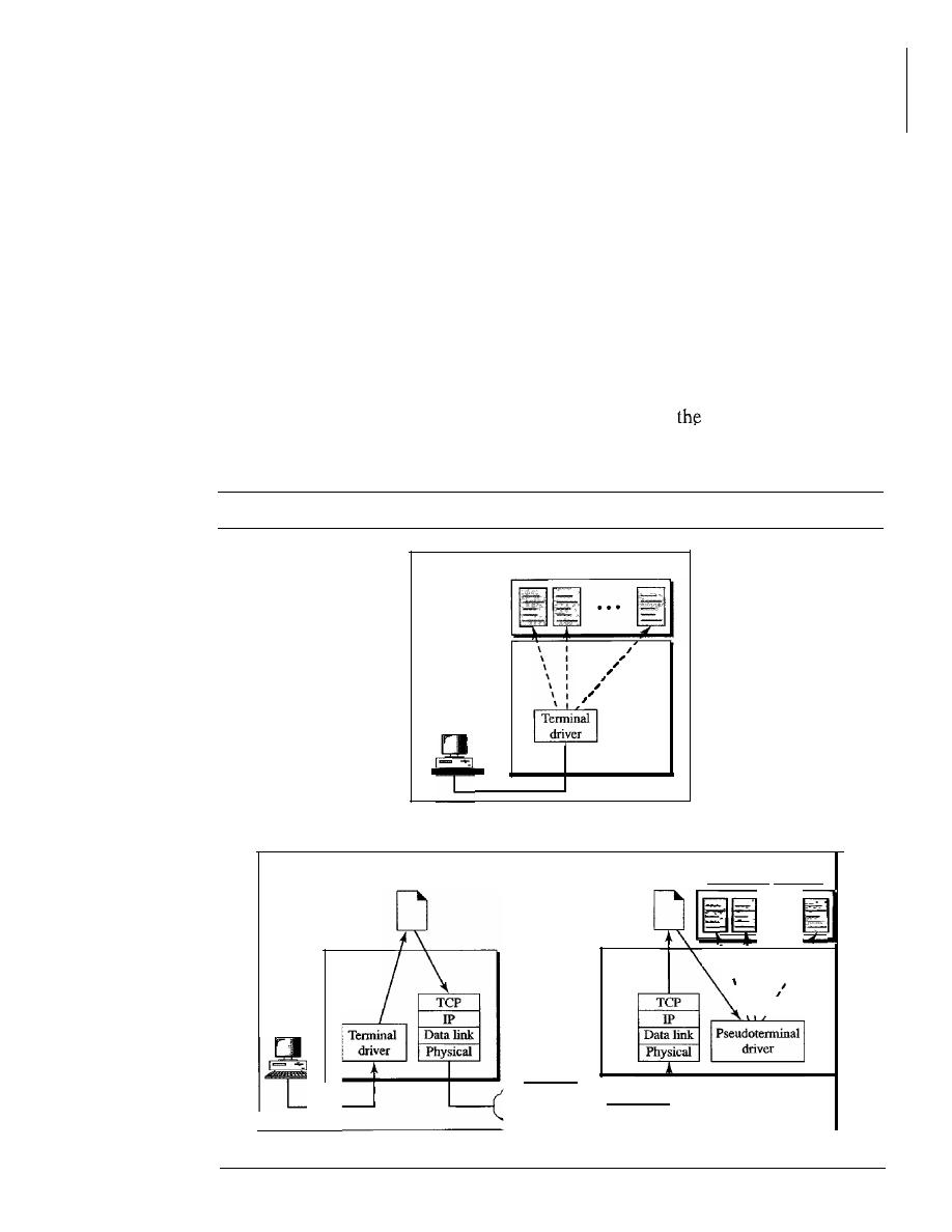
818
CHAPTER
26
REMOTE LOGGING, ELECTRONIC MAIL, AND FILE TRANSFER
Timesharing Environment
TELNET was designed at a time when most operating systems, such as UNIX, were
operating in a timesharing environment. In such an environment, a large computer
supports multiple users. The interaction between a user and the computer occurs through
a terminal, which is usually a combination of keyboard, monitor, and mouse. Even a
microcomputer can simulate a terminal with a terminal emulator.
Logging
In a timesharing environment, users are part of the system with some right to access
resources. Each authorized user has an identification and probablY,a password. The user
identification defines the user as part of the system. To access the system, the user logs
into the system with a user id or log-in name. The system also includes password
checking to prevent an unauthorized user from accessing
resources. Figure 26.1
shows the logging process.
Figure 26.1
Local and remote log-in
Application programs
Operating
system
...
Tenninal
a. Local log-in
TELNET
\
I
\
I
I
\
I
I
1 • • •
1
\
I
\
I
I
\ I
I
Application programs
...
server
Operating
system
Internet
TELNET
client
Operating
system
Tenninal
b. Remote log-in

SECTION
26.1
REMOTE LOGGING
819
When a user logs into a local timesharing system, it is called local log-in. As a user
types at a terminal or at a workstation running a terminal emulator, the keystrokes are
accepted by the terminal driver. The terminal driver passes the characters to the operat-
ing system. The operating system, in turn, interprets the combination of characters and
invokes the desired application program or utility.
When a user wants to access an application program or utility located on a remote
machine, she performs remote log-in. Here the TELNET client and server programs
come into use. The user sends the keystrokes to the terminal driver, where the local
operating system accepts the characters but does not interpret them. The characters are
sent to the TELNET client, which transforms the characters to a universal character set
called
network virtual terminal (NVT) characters
and delivers them to the local
TCP/IP
protocol stack.
The commands or text, in NVT form, travel through the Internet and arrive at the
TCP/IP stack at the remote machine. Here the characters are delivered to the operat-
ing system and passed to the TELNET server, which changes the characters to the
corresponding characters understandable by the remote computer. However, the char-
acters cannot be passed directly to the operating system because the remote operating
system is not designed to receive characters from a TELNET server:
It
is designed to
receive characters from a terminal driver. The solution is to add a piece of software
called a
pseudoterminal driver
which pretends that the characters are coming from
a terminal. The operating system then passes the characters to the appropriate appli-
cation program.
Network Virtual Terminal
The mechanism to access a remote computer is complex. This is so because every com-
puter and its operating system accept a special combination of characters as tokens. For
example, the end-of-file token in a computer running the DOS operating system is
Ctrl+z, while the UNIX operating system recognizes Ctrl+d.
We are dealing with heterogeneous systems.
If
we want to access any remote com-
puter in the world, we must first know what type of computer we will be connected to,
and we must also install the specific terminal emulator used by that computer. TELNET
solves this problem by defining a universal interface called the network virtual termi-
nal (NVT) character set. Via this interface, the client TELNET translates characters
(data or commands) that come from the local terminal into NVT form and delivers them
to the network. The server TELNET, on the other hand, translates data and commands
from NVT form into the form acceptable by the remote computer. For an illustration of
this concept, see Figure 26.2.
NVT Character Set
NVT uses two sets of characters, one for data and the other
for control. Both are 8-bit bytes. For data, NVT is an 8-bit character set in which the
7 lowest-order bits are the same as ASCII and the highest-order bit is O. To send control
characters between computers (from client to server or vice versa), NVT uses an 8-bit
character set in which the highest-order bit is set to
l.
Table 26.1 lists some of the control characters and their meanings.
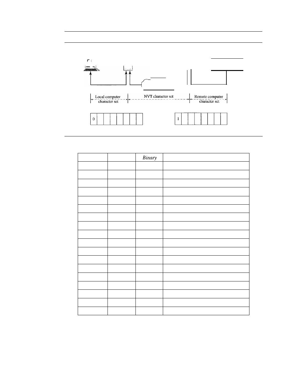
820
CHAPTER
26
REMOTE LOGGING, ELECTRONIC MAIL, AND FILE TRANSFER
Figure 26.2
Concept ofNVT
Terminal
TELNET
client
Internet
TELNET
server
Pseudoterminal
driver
Data character
Table
26.1
Some NVT control characters
Control character
Character
Decimal
Meaning
EOF
236
11101100
End of file
EOR
239
11101111
End of record
SE
240
11110000
Suboption end
NOP
241
11110001
No operation
DM
242
11110010
Data mark
BRK
243
11110011
Break
IP
244
11110100
Interrupt process
AO
245
11110101
Abort output
AYT
246
11110110
Are you there?
EC
247
11110111
Erase character
EL
248
11111000
Erase line
GA
249
11111001
Go ahead
SB
250
11111010
Suboption begin
WILL
251
11111011
Agreement to enable option
WONT
252
11111100
Refusal to enable option
DO
253
11111101
Approval to option request
DONT
254
11111110
Denial of option request
lAC
255
11111111
Interpret (the next character) as control
Embedding
TELNET uses only one TCP connection. The server uses the well-known port 23, and
the client uses an ephemeral port. The same connection is used for sending both data and
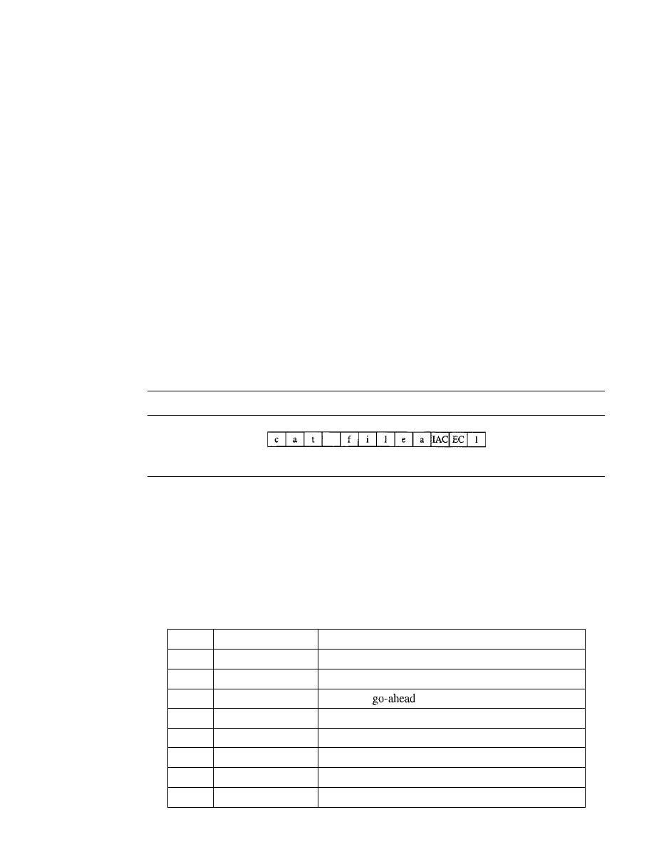
SECTION 26.1
REMOTE LOGGING
821
control characters. TELNET accomplishes this by embedding the control characters in the
data stream. However, to distinguish data from control characters, each sequence of con-
trol characters is preceded by a special control character called interpret as control (lAC).
For example, imagine a user wants a server to display a file
(filel)
on a remote server.
She can type
catfilel
However, suppose the name of the file has been mistyped (filea instead of filel). The
user uses the backspace key to correct this situation.
catjllea<backspace>l
However, in the default implementation of TELNET, the user cannot edit locally; the
editing is done at the remote server. The backspace character is translated into two
remote characters (lAC EC), which are embedded in the data and sent to the remote
server. What is sent to the server is shown in Figure 26.3.
Figure 26.3
An example ofembedding
Typed at the remote terminal
Options
TELNET lets the client and server negotiate options before or during the use of the ser-
vice. Options are extra features available to a user with a more sophisticated terminal.
Users with simpler terminals can use default features. Some control characters discussed
previously are used to define options. Table 26.2 shows some common options.
Table 26.2
Options
Code
Option
Meaning
0
Binary
Interpret as 8-bit binary transmission.
1
Echo
Echo the data received on one side to the other.
3
Suppress go ahead
Suppress
signals after data.
5
Status
Request the status of TELNET.
6
Timing mark
Define the timing marks.
24
Terminal type
Set the terminal type.
32
Terrninalspeed
Set the terminal speed.
34
Line mode
Change to line mode.

822
CHAPTER
26
REMOTE LOGGING, ELECTRONIC MAIL, AND FILE TRANSFER
Option Negotiation
To use any of the options mentioned in the previous section first
requires option negotiation between the client and the server. Four control characters
are used for this purpose; these are shown in Table 26.3.
Table 26.3
NVT character set for
negotiation
Character
Decimal
Binary
Meaning
WILL
251
11111011
1. Offering to enable
2. Accepting a request to enable
WONT
252
11111100
1. Rejecting a request to enable
2. Offering to disable
3. Accepting a request to disable
DO
253
11111101
1. Approving an offer to enable
2. Requesting to enable
DONT
254
11111110
1. Disapproving an offer to enable
2. Approving an offer to disable
3. Requesting to disable
A party can offer to enable or disable an option if it has the right to do so. The
offering can be approved or disapproved by the other party. To offer enabling, the offer-
ing party sends the WILL command, which means "Will I enable the option?" The
other party sends either the DO command, which means "Please do," or the DONT
command, which means "Please don't." To offer disabling, the offering party sends the
WONT command, which means "I won't use this option any more." The answer must
be the DONT command, which means "Don't use it anymore."
A party can request from the other party the enabling or the disabling of an option.
To request enabling, the requesting party sends the DO command, which means
"Please do enable the option." The other party sends either the WILL command, which
means "I will," or the WONT command, which means "I won't." To request disabling,
the requesting party sends the DONT command, which means "Please don't use this
option anymore." The answer must be the WONT command, which means "I won't use
it anymore."
Example 26.1
Figure 26.4 shows an example of option negotiation. In this example, the client wants the server to
echo each character sent to the server. In other words, when a character is typed at the user keyboard
terminal, it goes to the server and is sent back to the screen of the user before being processed. The
echo option is enabled by the server because it is the server that sends the characters back to the user
tenninal. Therefore, the client should request from the server the enabling of the option using DO.
The request consists of three characters: lAC, DO, and ECHO. The server accepts the request
enables the option.
It
informs the client by sending the three-character approval: lAC, WILL,
and ECHO.
Suboption Negotiation
Some options require additional information. For example,
to define the type or speed of a terminal, the negotiation includes a string or a number
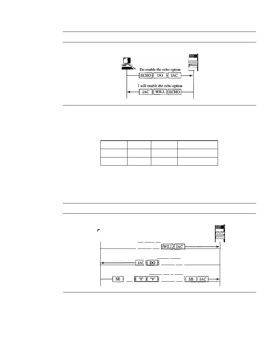
SECTION
26.1
REMOTE LOGGING
823
Figure 26.4
Example
26.1:
Echo option
Client
Server
-
to define the type or speed. In either case, the two suboption characters indicated
in Table 26.4 are needed for suboption negotiation.
Table 26.4
NVT character set for suboption negotiation
Character
Decimal
Binary
Meaning
SE
240
11110000
Suboption end
SB
250
11111010
Suboption begin
Example 26.2
Figure 26.5 shows an example of suboption negotiation. In this example, the client wants to
negotiate the type of the terminal.
Figure 26.5
Example of suboption negotiation
Server
-
I
will enable the terminal option
1-------1
Terminal type
Client
Do enable terminal option
Terminal type
1------1
Set the terminal type to "VT"
I
rAC
Terminal type
Mode of Operation
Most TELNET implementations operate in one of three modes: default mode, character
mode, or line mode.
Default Mode
The default mode is used if no other modes are invoked through
option negotiation. In this mode, the echoing is done by the client. The user types a

824
CHAPTER
26
REMOTE LOGGING, ELECTRONIC MAIL, AND FILE TRANSFER
character, and the client echoes the character on the screen (or printer) but does not
send it until a whole line is completed.
Character Mode
In the character mode, each character typed is sent by the client to
the server. The server normally echoes the character back to be displayed on the client
screen. In this mode the echoing of the character can be delayed if the transmission
time is long (such as in a satellite connection).
It
also creates overhead (traffic) for the
network because three TCP segments must be sent for each character of data.
Line Mode
A new mode has been proposed to compensate for the deficiencies of the
default mode and the character mode. In this mode, called the line mode, line editing
(echoing, character erasing, line erasing, and so on) is done by the client. The client
then sends the whole line to the server.
26.2
ELECTRONIC MAIL
One of the most popular Internet services is electronic mail (e-mail). The designers of
the Internet probably never imagined the popularity of this application program. Its
architecture consists of several components that we discuss in this chapter.
At the beginning of the Internet era, the messages sent by electronic mail were short
and consisted of text only; they let people exchange quick memos. Today, electronic
mail is much more complex. It allows a message to include text, audio, and video. It also
allows one message to be sent to one or more recipients.
In this chapter, we first study the general architecture of an e-mail system including
the three main components: user agent, message transfer agent, and message access
agent. We then describe the protocols that implement these components.
Architecture
To explain the architecture of e-mail, we give four scenarios. We begin with the simplest
situation and add complexity as we proceed. The fourth scenario is the most common in
the exchange of email.
First Scenario
In the first scenario, the sender and the receiver of the e-mail are users (or application
programs) on the same system; they are directly connected to a shared system. The
administrator has created one mailbox for each user where the received messages are
stored. A
mailbox
is part of a local hard drive, a special file with permission restrictions.
Only the owner of the mailbox has access to it. When Alice, a user, needs to send a
message to Bob, another user, Alice runs a
user agent (VA)
program to prepare the
message and store it in Bob's mailbox. The message has the sender and recipient mail-
box addresses (names of files). Bob can retrieve and read the contents of his mailbox at
his convenience, using a user agent. Figure 26.6 shows the concept.
This is similar to the traditional memo exchange between employees in an office.
There is a mailroom where each employee has a mailbox with his or her name on it.
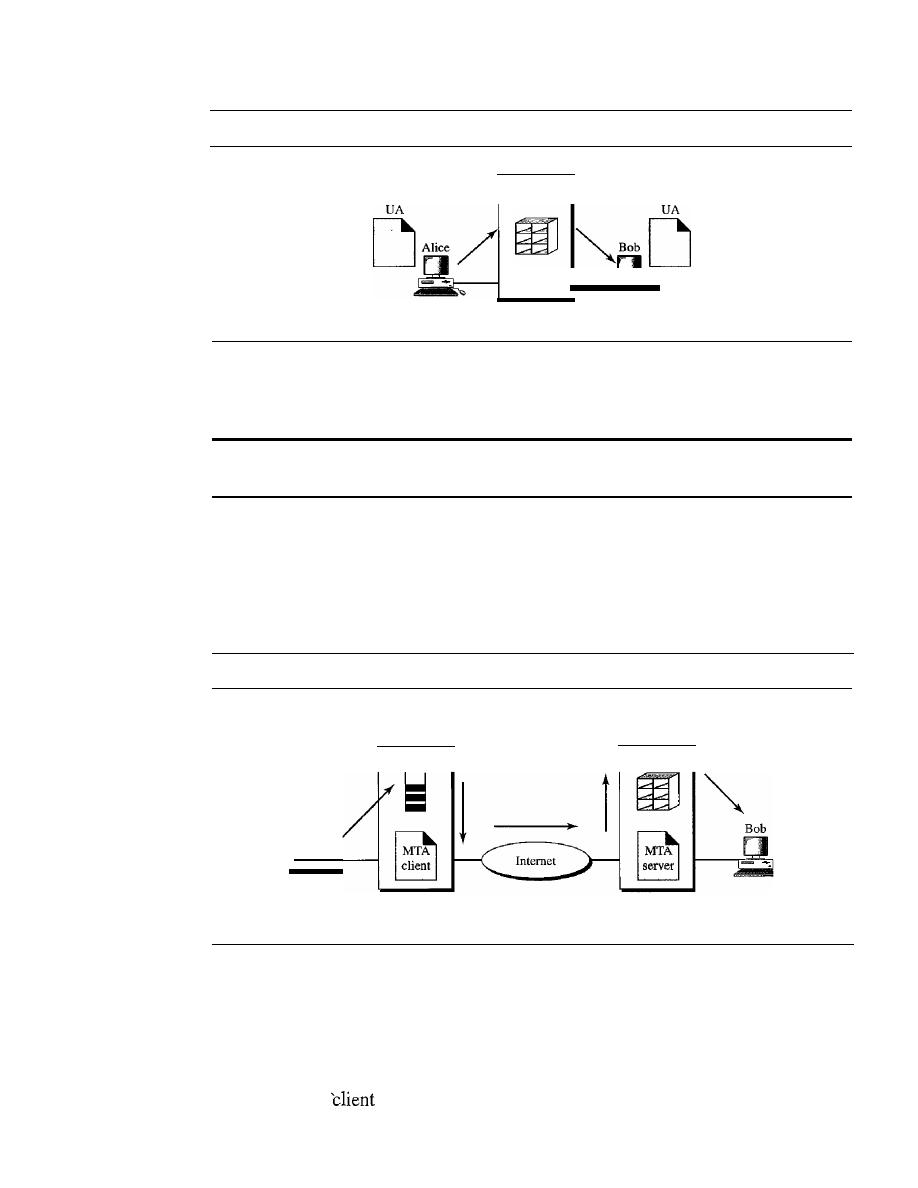
SECTION
26.2
ELECTRONIC MAIL
825
Figure 26.6
First scenario in electronic mail
VA: user agent
System
When Alice needs to send a memo to Bob, she writes the memo and inserts it into
Bob's mailbox. When Bob checks his mailbox, he finds Alice's memo and reads it.
When the sender and the receiver of an e-mail are on the same system,
we need only two user agents.
Second Scenario
In the second scenario, the sender and the receiver of the e-mail are users (or application
programs) on two different systems.The message needs to be sent over the Internet. Here we
need
user agents
(VAs) and
message transfer agents
(MTAs),
as shown
in
Figure 26.7.
Figure 26.7
Second scenario in electronic mail
VA: user agent
MTA: message transfer agent
VA
D
System
(mail server)
System
(mail server)
VA
D
Alice needs to use a user agent program to send her message to the system at her
own site. The system (sometimes called the mail server) at her site uses a queue to store
messages waiting to be sent. Bob also needs a user agent program to retrieve messages
stored in the mailbox of the system at his site. The message, however, needs to be sent
through the Internet from Alice's site to Bob's site. Here two message transfer agents
are needed: one
and one server. Like most client/server programs on the Internet,
the server needs to run all the time because it does not know when a client will ask for a
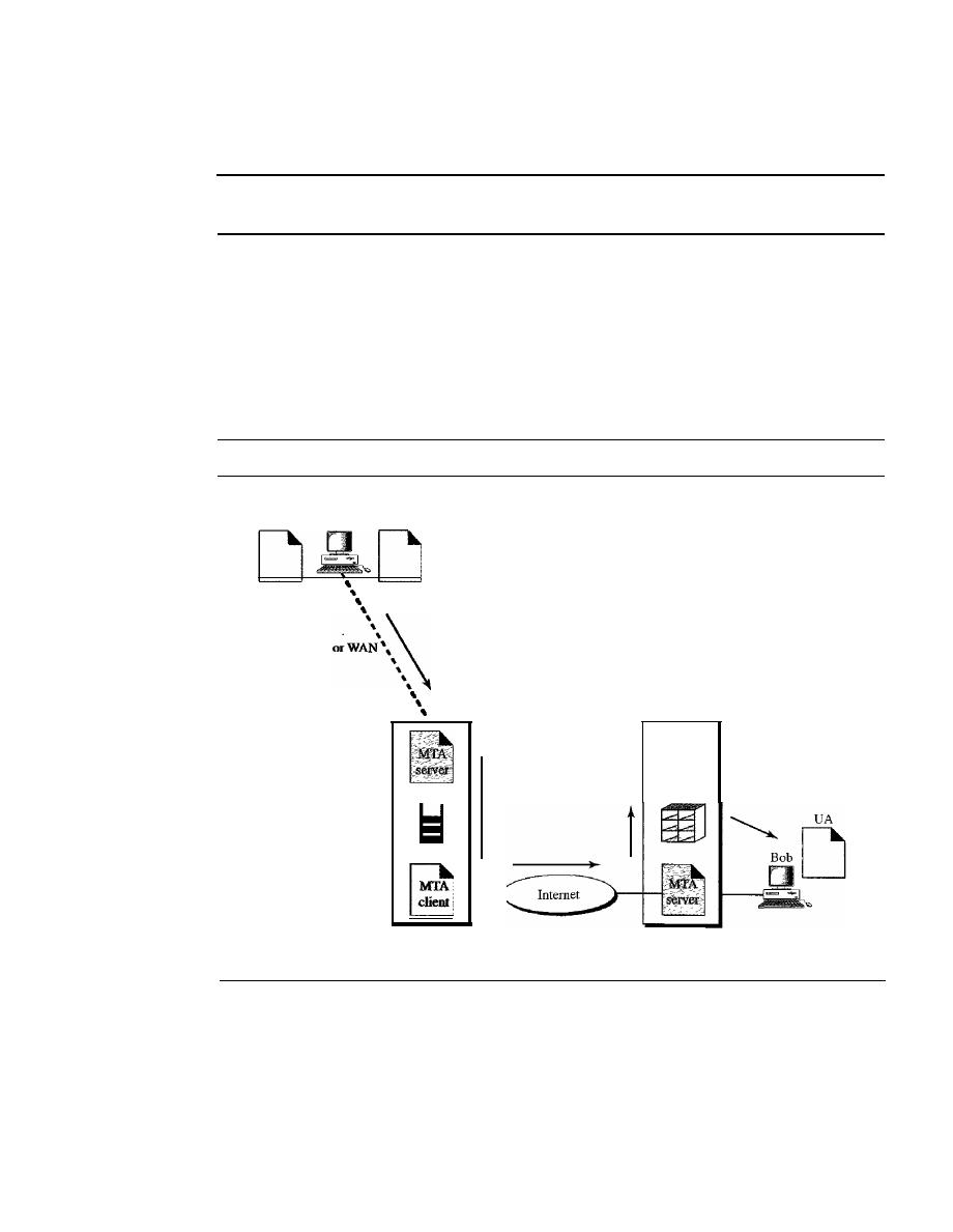
826
CHAPTER
26
REMOTE LOGGING, ELECTRONIC MAIL, AND FILE TRANSFER
connection. The client, on the other hand, can be alerted by the system when there is a
message in the queue to be sent.
When the sender and the receiver of an e-mail are on different systems,
we need two VAs and a pair ofMTAs (client and server).
Third Scenario
In the third scenario, Bob, as in the second scenario, is directly connected to his system.
Alice, however, is separated from her system. Either Alice is connected to the system via
a point-to-point WAN, such as a dial-up modem, a DSL, or a cable modem; or she is con-
nected to a LAN in an organization that uses one mail server for handling e-mails-all
users need to send their messages to this mail server. Figure 26.8 shows the situation.
Figure 26.8
Third scenario in electronic mail
MTA
VA
Alice
client
LAN
System
(mail server)
VA:
user agent
MTA: message transfer agent
System
(mail server)
Alice still needs a user agent to prepare her message. She then needs to send the
message through the LAN or WAN. This can be done through a pair of message transfer
agents (client and server). Whenever Alice has a message to send, she calls the user
agent which, in tum, calls the MTA client. The MTA client establishes a connection
with the MTA server on the system, which is running all the time. The system at Alice's
site queues all messages received. It then uses an MTA client to send the messages to
the system at Bob's site; the system receives the message and stores it in Bob's mailbox.
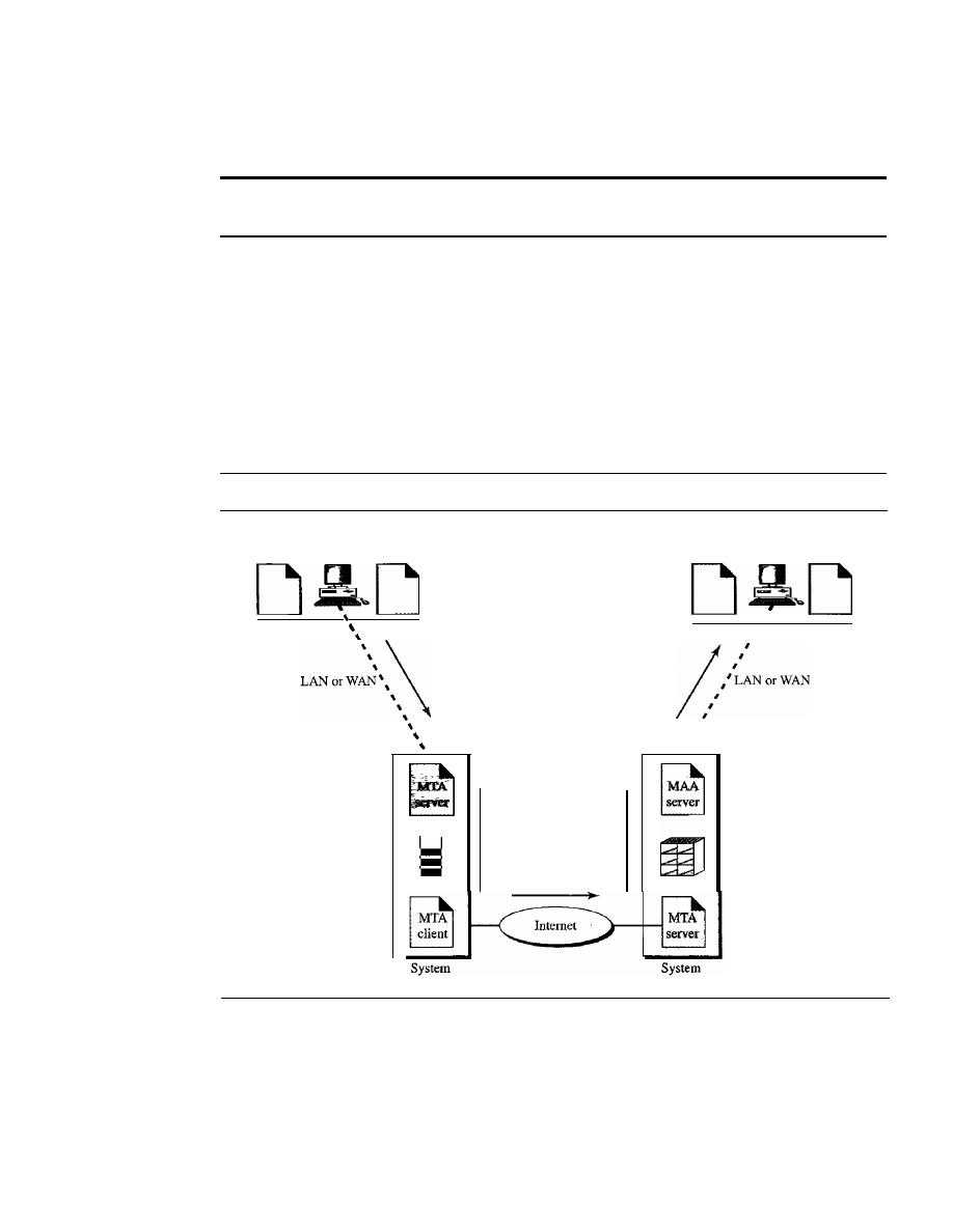
SECTION
26.2
ELECTRONIC MAIL
827
At his convenience, Bob uses his user agent to retrieve the message and reads it. Note
that we need two pairs of MTA client/server programs.
When the sender is connected to the mail server via a LAN or a WAN,
we need two
VAs and two paIrs of MTAs (clIent and server).
Fourth Scenario
In the fourth and most common scenario, Bob is also connected to his mail server by a
WAN or a LAN. After the message has arrived at Bob's mail server, Bob needs to retrieve
it. Here, we need another set of client/server agents, which we call message access
agents (MAAs). Bob uses an MAA client to retrieve his messages. The client sends a
request to the MAA server, which is running all the time, and requests the transfer of the
messages. The situation is shown in Figure 26.9.
Figure 26.9
Fourth scenario in electronic mail
MTA
UA
Alice
client
UA: user agent
MTA: message transfer agent
MAA: message access agent
MAA
client
Bob
UA
,
,
,
,
,
,
There are two important points here. First, Bob cannot bypass the mail server and
use the MTA server directly. To use MTA server directly, Bob would need to run the
MTA server all the time because he does not know when a message will arrive. This
implies that Bob must keep his computer on all the time if he is connected to his system
through a LAN.
If
he is connected through a-WAN, he must keep the connection up all
the time. Neither of these situations is feasible today.
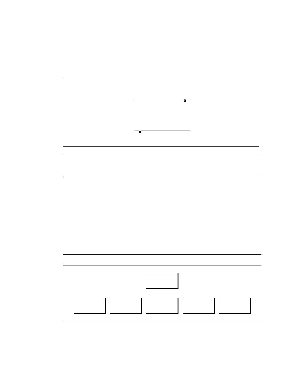
828
CHAPTER
26
REMOTE LOGGING, ELECTRONIC MAIL, AND FILE TRANSFER
Second, note that Bob needs another pair of client/server programs: message
access programs. This is so because an MTA client/server program is a
push
program:
the client pushes the message to the server. Bob needs a
pull
program. The client needs
to pull the message from the server. Figure 26.10 shows the difference.
Figure 26.10
Push versus pull in electronic email
MTA
MTA
client
server
D
Client pushes messages
D
MAA
MAA
client
server
D
Client pulls messages
D
When both sender and receiver are connected to the mail server via a LAN or a WAN,
we need two VAs, two pairs of MTAs (client and server), and a pair of MAAs
(client and server). This is the most common situation today.
User Agent
The first component of an electronic mail system is the user agent
(VA).
It
provides
service to the user to make the process of sending and receiving a message easier.
Services Provided by a User Agent
A user agent is a software package (program) that composes, reads, replies to, and for-
wards messages.
It
also handles mailboxes. Figure 26.11 shows the services of a typical
user agent.
Figure 26.11
Services of user agent
User agent
I
I
I
I
I
I
Composing
Reading
Replying to
Forwarding
Handling
messages
messages
messages
messages
mailboxes
Composing Messages
A user agent helps the user compose the e-mail message to be
sent out. Most user agents provide a template on the screen to be filled in by the user.
Some even have a built-in editor that can do spell checking, grammar checking, and

SECTION 26.2
ELECTRONIC MAIL
829
other tasks expected from a sophisticated word processor. A user, of course, could alter-
natively use his or her favorite text editor or word processor to create the message and
import it, or cut and paste it, into the user agent template.
Reading Messages
The second duty of the user agent is to read the incoming mes-
sages. When a user invokes a user agent, it first checks the mail in the incoming mailbox.
Most user agents show a one-line summary of each received mail. Each e-mail contains
the following fields.
1. A number field.
2. A flag field that shows the status of the mail such as new, already read but not
replied to, or read and replied to.
The size of the message.
4. The sender.
5.
The optional subject field.
Replying to Messages
After reading a message, a user can use the user agent to reply
to a message. A user agent usually allows the user to reply to the original sender or to
reply to all recipients of the message. The reply message may contain the original mes-
sage (for quick reference) and the new message.
Forwarding Messages
Replying
is defined as sending a message to the sender or
recipients of the copy. Forwarding is defined as sending the message to a third party. A
user agent allows the receiver to forward the message, with or without extra comments,
to a third party.
Handling Mailboxes
A user agent normally creates two mailboxes: an inbox and an outbox. Each box is a file
with a special format that can be handled by the user agent. The inbox keeps all the received
e-mails until they are deleted by the user. The outbox keeps all the sent e-mails until the
user deletes them. Most user agents today are capable of creating customized mailboxes.
User Agent Types
There are two types of user agents: command-driven and GUI-based.
Command-Driven
Command-driven user agents belong to the early days of electronic
mail. They are still present as the underlying user agents in servers. A command-driven
user agent normally accepts a one-character command from the keyboard to perform its
task. For example, a user can type the character r, at the command prompt, to reply to the
sender of the message, or type the character R to reply to the sender and all recipients.
Some examples of command-driven user agents are mail, pine, and elm.
Some examples of command-driven user agents are
mail, pine,
and
elm.
GUI-Based
Modem user agents are GUI-based. They contain graphical-user inter-
face (GUI) components that allow the user to interact with the software by using both
the keyboard and the mouse. They have graphical components such as icons, menu
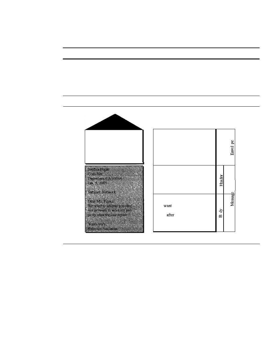
830
CHAPTER
26
REMOTE LOGGING, ELECTRONIC MAIL, AND FILE TRANSFER
bars, and windows that make the services easy to access. Some examples of GUI-based
user agents are Eudora, Microsoft's Outlook, and Netscape.
Some examples of GUI·based user agents are
Eudora, Outlook, and Netscape.
Sending Mail
To send mail, the user, through the UA, creates mail that looks very similar to postal
mail.
It
has an envelope and a message (see Figure 26.12).
Figure 26.12
Format of an e-mail
Behrollz Forouzan
De Anza College
Cupertino, CA 96014
Sophia Fegan
Com-Net
Cupertino, CA 95014
a. Postal mail
Mail From: forouzan@deanza.edu
0
RCPT To: fegan@comnet.com
From: Behrouz Forouzan
TQ:
Sophia Fegan
Date:
liS/OS
Subject: Network
Dear
Ms. Fegan:
We
to
inform you that
our network is working pro-
perly
the last repair.
0
Yours truly, .
Behrouz Porouzan
b. Electromc mall
Envelope
The envelope usually contains the sender and the receiver addresses.
Message
The message contains the header and the body. The header of the message
defines the sender, the receiver, the subject of the message, and some other information
(such as encoding type, as we see shortly). The body of the message contains the actual
information to be read by the recipient.
Receiving Mail
The user agent is triggered by the user (or a timer).
If
a user has mail, the
VA
informs
the user with a notice.
If
the user is ready to read themail.alist is displayed in which
each line contains a summary of the information about a particular message in the mail-
box. The summary usually includes the sender mail address, the subject, and the time
the mail was sent or received. The user can select any of the messages and display its
contents on the screen.
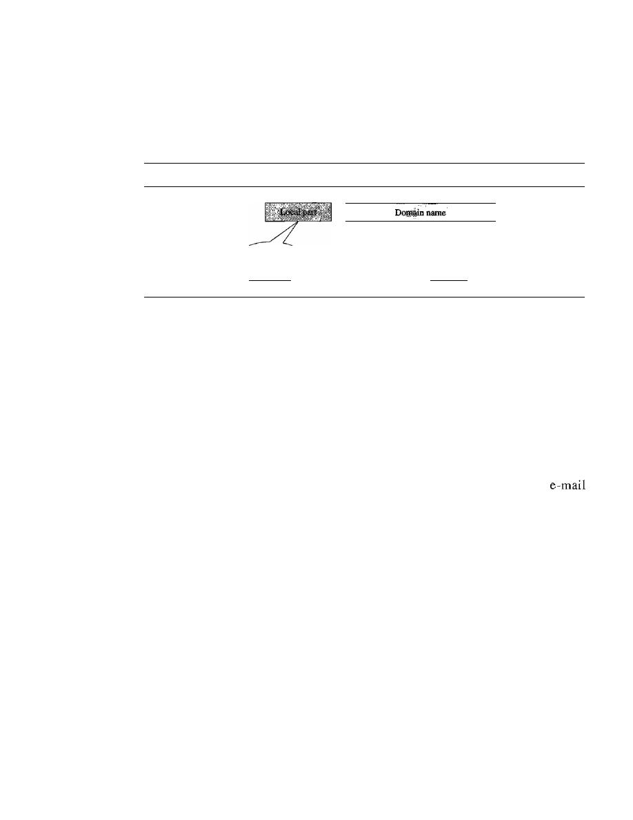
SECTION
26.2
ELECTRONIC MAIL
831
Addresses
To deliver mail, a mail handling system must use an addressing system with unique
addresses. In the Internet, the address consists of two parts: a local part and a domain
name, separated by an
@
sign (see Figure 26.13).
Figure 26.13
E-mail address
Address of the
mailbox on the
mail server
@
The domain
name of the
mail server
Local Part
The local part defines the name of a special file, called the user mailbox,
where all the mail received for a user is stored for retrieval by the message access agent.
Domain Name
The second part of the address is the domain name.
An
organization
usually selects one or more hosts to receive and send e-mail; the hosts are sometimes
called
mail servers
or
exchangers.
The domain name assigned to each mail exchanger
either comes from the DNS database or is a logical name (for example, the name of the
organization).
Mailing List
Electronic mail allows one name, an alias, to represent several different
addresses; this is called a mailing list. Every time a message is to be sent, the system
checks the recipient's name against the alias database; if there is a mailing list for the
defined alias, separate messages, one for each entry in the list, must be prepared and
handed to the MTA.
If
there is no mailing list for the alias, the name itself is the receiving
address and a single message is delivered to the mail transfer entity.
MIME
Electronic mail has a simple structure. Its simplicity, however, comes at a price. It can
send messages only in NVT 7-bit ASCII format. In other words, it has some limita-
tions. For example, it cannot be used for languages that are not supported by 7-bit
ASCII characters (such as French, German, Hebrew, Russian, Chinese, and Japanese).
Also, it cannot be used to send binary files or video or audio data.
Multipurpose Internet Mail Extensions (MIME) is a supplementary protocol that
allows non-ASCII data to be sent through e-mail. MIME transforms non-ASCII data at
the sender site to NVT ASCII data and delivers them to the client MTA to be sent through
the Internet. The message at the receiving side is transformed back to the original data.
We can
think
of MIME as a set of software functions that transforms non-ASCII
data (stream of bits) to ASCII data and vice versa, as shown in Figure 26.14.
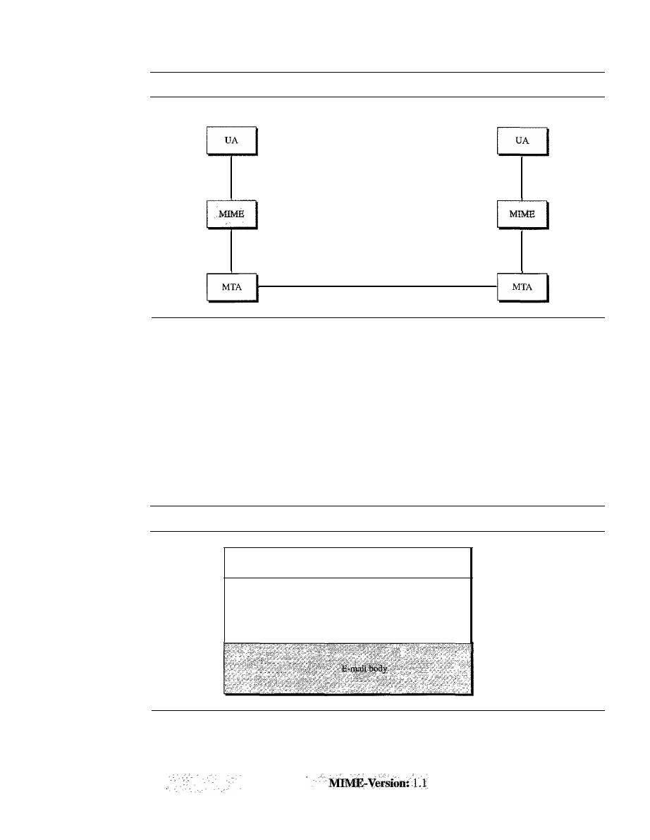
832
CHAPTER
26
REMOTE LOGGING, ELECTRONIC MAIL, AND FILE TRANSFER
Figure 26.14
MIME
User
Non-ASCII code
7-bit NVT ASCII
7-bit NVT ASCII
User
Non-ASCII code
7-bit NVT ASCII
MIME defines five headers that can be added to the original e-mail header section
to define the transformation parameters:
1.
MIME-Version
2.
Content-Type
3. Content-Transfer-Encoding
4. Content-Id
5.
Content-Description
Figure 26.15 shows the MIME headers. We will describe each header in detail.
Figure 26.15
MIME header
E-mail header
MIME-Version:
1.1
Content-Type: type/subtype
Content-Transfer-Encoding: encoding type
MIME headers
Content-Id: message id
Content-Description: textual explanation of nontextual contents
MIME-Version
This header defines the version of MIME used. The current version
is
1.1.

SECTION
26.2
ELECTRONIC MAIL
833
Content-Type
This header defines the type of data used in the body of the message.
The content type and the content subtype are separated by a slash. Depending on the
subtype, the header may contain other parameters.
J
MIME allows seven different types of data. These are listed in Table 26.5.
Table 26.5
Data types and subtypes in MIME
Type
Subtype
Description
Text
Plain
Unformatted
HTML
HTML format (see Chapter 27)
Mixed
Body contains ordered parts of different data types
Multipart
Parallel
Same as above, but no order
Digest
Similar to mixed subtypes, but the default is message/
RFC822
Alternative
Parts are different versions of the same message
RFC822
Body is an encapsulated message
Message
Partial
Body is a fragment of a bigger message
External-Body
Body is a reference to another message
Image
IPEG
Image is in IPEG format
GIF
Image is in GIF format
Video
MPEG
Video is in MPEG format
Audio
Basic
Single-channel encoding of voice at 8 kHz
Application
PostScript
Adobe PostScript
Octet-stream
General binary data (8-bit bytes)
Content-Transfer-Encoding
This header defines the method used to encode the
messages into Os and Is for transport:
The five types of encoding methods are listed in Table 26.6.
Content-Id
This header uniquely identifies the whole message in a multiple-message
environment.
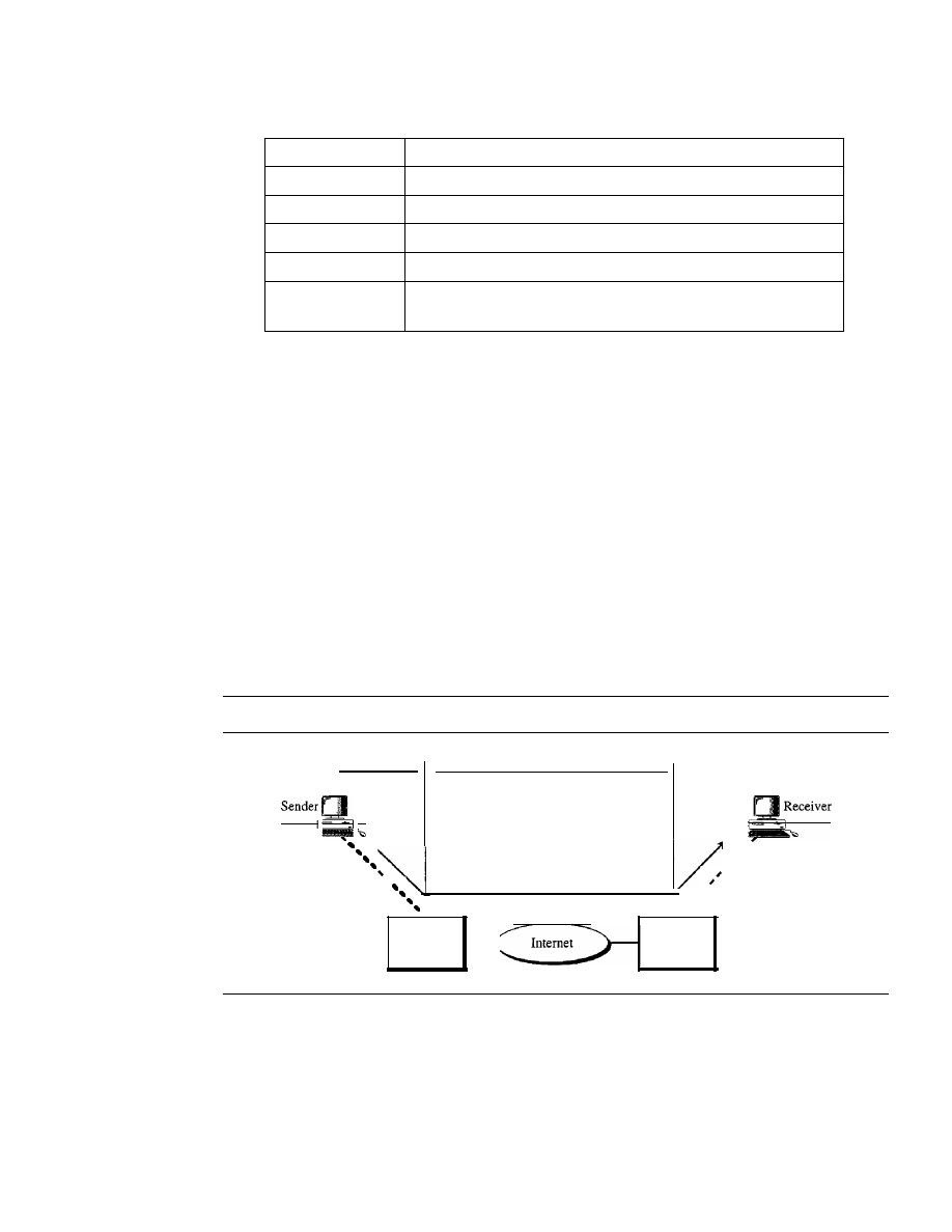
834
CHAPTER
26
REMOTE LOGGING, ELECTRONIC MAIL, AND FILE TRANSFER
Table 26.6
Content-transfer-encoding
Type
Description
7-bit
NVT ASCII characters and short lines
8-bit
Non-ASCII characters and short lines
Binary
Non-ASCII characters with unlimited-length lines
Base-64
6-bit blocks of data encoded into 8-bit ASCII characters
Quoted-printable
Non-ASCII characters encoded as an equals sign followed
by an ASCII code
Content-Description
This header defines whether the body is image, audio, or video.
Content-Description:
<description>
Message Transfer Agent: SMTP
The actual mail transfer is done through message transfer agents. To send mail, a system
must have the client MTA, and to receive mail, a system must have a server MTA. The
formal protocol that defines the MTA client and server in the Internet is called the
Simple
Mail Transfer Protocol (SMTP).
As we said before, two pairs of MTA client/server
programs are used in the most common situation (fourth scenario). Figure 26.16 shows
the range of the SMTP protocol in this scenario.
Figure
26.16
SMTP range
SMTP
SMTP
,
,
,
,
LAN
or
WAN
,
,
,
,
LAN
or
WAN
server
server
SMTP is used two times, between the sender and the sender's mail server and
between the two mail servers. As we will see shortly, another protocol is needed
between the mail server and the receiver.
SMTP simply defines how commands and responses must be sent back and forth.
Each network is free to choose a software package for implementation. We discuss the
mechanism of mail transfer by SMTP in the remainder of the section.
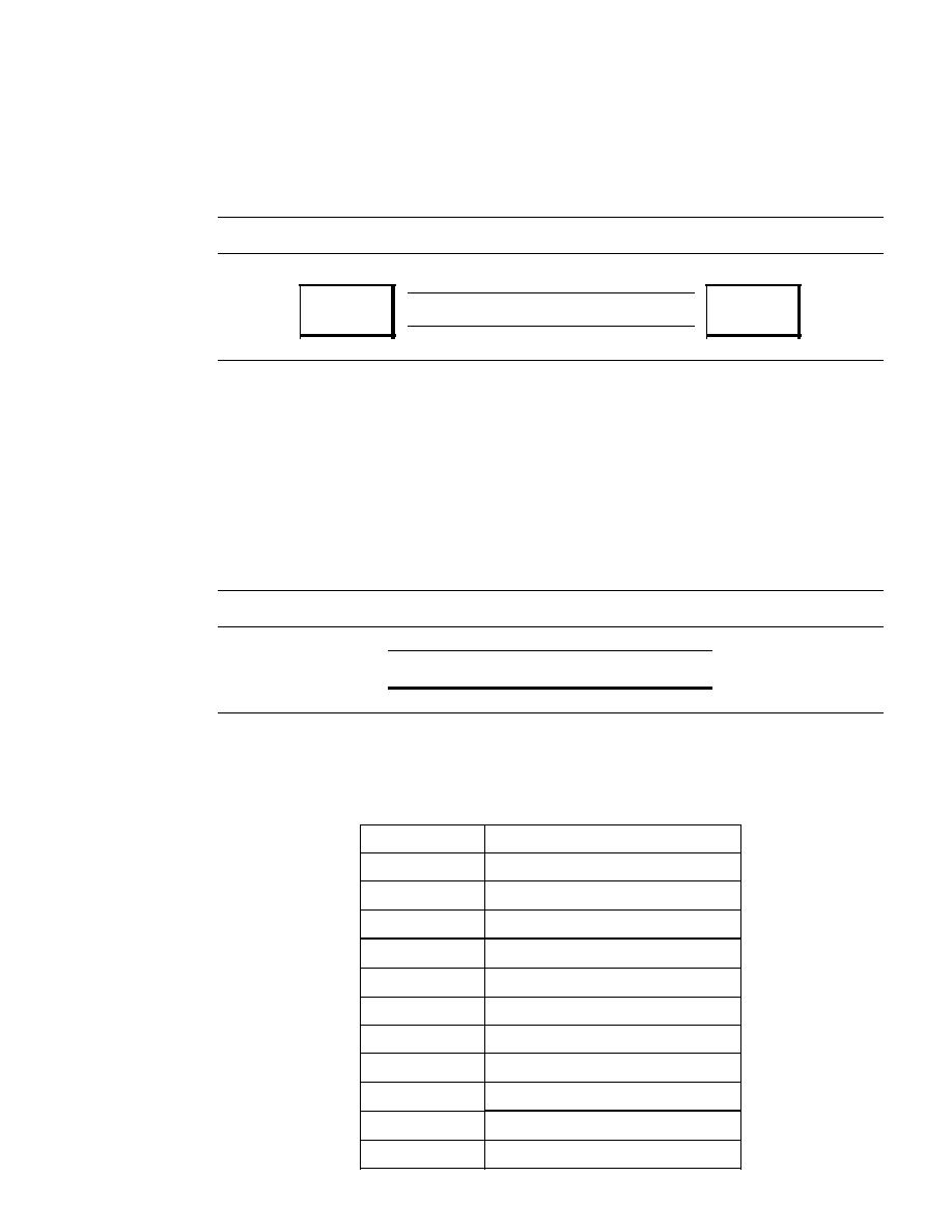
SECTION 26.2
ELECTRONIC MAIL
835
Commands and Responses
SMTP uses commands and responses to transfer messages between an MTA client and
an MTA server (see Figure 26.17).
Figure 26.17
Commands and responses
Commands
MTA
client
Responses
MTA
server
Each command or reply is terminated by a two-character (carriage return and line feed)
end-of-line token.
Commands
Commands are sent from the client to the server. The fonnat of a command
is shown in Figure 26.18.
It
consists of a keyword followed by zero or more arguments.
SMTP defines 14 commands. The first five are mandatory; every implementation must
support these five commands. The next three are often used and highly recommended. The
last six are seldom used.
Figure 26.18
Commandformat
Keyword: argument(s)
The commands are listed in Table 26.7.
Table 26.7
Commands
Keyword
Argument(s)
HELO
Sender's host name
MAIL FROM
Sender of the message
RCPTTO
Intended recipient of the message
DATA
Body of the mail
QUIT
RSET
VRFY
Name of recipient to be verified
NOOP
TURN
EXPN
Mailing list to be expanded
HELP
Command name

836
CHAPTER
26
REMOTE LOGGING, ELECTRONIC MAIL, AND FILE TRANSFER
Table 26.7
Commands (continued)
Keyword
Argument(s)
SEND FROM
Intended recipient of the message
SMOLFROM
Intended recipient of the message
SMALFROM
Intended recipient of the message
Responses
Responses are sent from the server to the client. A response is a three-
digit code that may be followed by additional textual information. Table 26.8 lists some
of the responses.
Table 26.8
Responses
Code
Description
Positive Completion Reply
211
System status or help reply
214
Help message
220
Service ready
221
Service closing transmission channel
250
Request command completed
251
User not local; the message will be forwarded
Positive Intermediate Reply
354
Start mail input
Transient Negative Completion Reply
421
Service not available
450
Mailbox not available
451
Command aborted: local error
452
Command aborted: insufficient storage
Permanent Negative Completion Reply
500
Syntax error; unrecognized command
501
Syntax error in parameters or arguments
502
Command not implemented
503
Bad sequence of commands
504
Command temporarily not implemented
550
Command is not executed; mailbox unavailable
551
User not local
552
Requested action aborted; exceeded storage location
553
Requested action not taken; mailbox name not allowed
554
Transaction failed
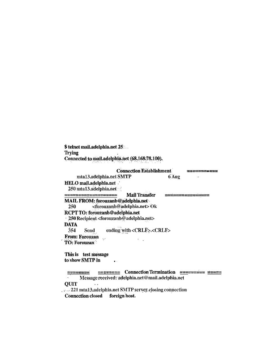
SECTION
26.2
ELECTRONIC MAIL
837
As the table shows, responses are divided into four categories. The leftmost digit of
the code (2, 3, 4, and
5)
defines the category.
Mail Transfer Phases
The process of transferring a mail message occurs in three phases: connection estab-
lishment, mail transfer, and connection termination.
Example 26.3
Let us see how we can directly use SMTP to send an e-mail and simulate the commands
and responses we described in this section. We use TELNET to log into port
25
(the weIl-
known port for SMTP). We then use the commands directly to send an e-mail. In this example,
forouzanb@adelphia.net is sending an e-mail to himself. The first few lines show TELNET try-
ing to connect to the Adelphia mail server.
After connection, we can type the SMTP commands and then receive the responses, as
shown below. We have shown the commands in black and the responses in color. Note that we
have added, for clarification, some comment lines, designated by the
"="
signs. These lines are
not part of the e-mail procedure.
68.168.78.100 •••
========
--
220
serverready
Fri,
2004 ...
Sender:
Ok
Ok
data
:
a
action
250
by
Message Access Agent:
POP
and IMAP
The first and the second stages of mail delivery use SMTP. However, SMTP is not
involved in the third stage because SMTP is a
push
protocol; it pushes the message from
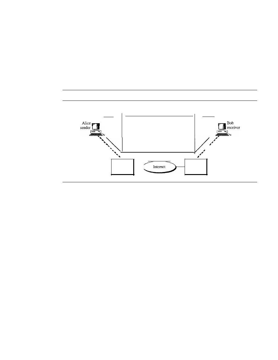
838
CHAPTER
26
REMOTE LOGGING, ELECTRONIC MAIL, AND FILE TRANSFER
the client to the server. In other words, the direction of the bulk: data (messages) is from
the client to the server. On the other hand, the third stage needs a pull protocol; the client
must pull messages from the server. The direction of the bulk data is from the server to
the client. The third stage uses a message access agent.
Currently two message access protocols are available: Post Office Protocol, version 3
(POP3) and Internet Mail Access Protocol, version 4 (IMAP4). Figure 26.19 shows the
position of these two protocols in the most common situation (fourth scenario).
Figure 26.19
POP3 and IMAP4
I
SMTP
LANorWAN
Mail server
SMTP
POP3
IMAP4
I
;;LANorWAN
Mail server
POP3
Post Office Protocol, version 3 (POP3)
is simple and limited in functionality. The
client POP3 software is installed on the recipient computer; the server POP3 software
is installed on the mail server.
Mail access starts with the client when the user needs to download e-mail from the
mailbox on the mail server. The client opens a connection to the server on TCP port 110.
It
then sends its user name and password to access the mailbox. The user can then list
and retrieve the mail messages, one by one. Figure 26.20 shows an example of down-
loading using POP3.
POP3 has two modes: the delete mode and the keep mode. In the delete mode, the
mail is deleted from the mailbox after each retrieval. In the keep mode, the mail
remains in the mailbox after retrieval. The delete mode is normally used when the user
is working at her permanent computer and can save and organize the received mail after
reading or replying. The keep mode is normally used when the user accesses her mail
away from her primary computer (e.g., a laptop). The mail is read but kept in the system
for later retrieval and organizing.
IMAP4
Another mail access protocol is
Internet Mail Access Protocol, version 4 (IMAP4).
IMAP4 is similar to POP3, but it has more features; IMAP4 is more powerful and more
complex.
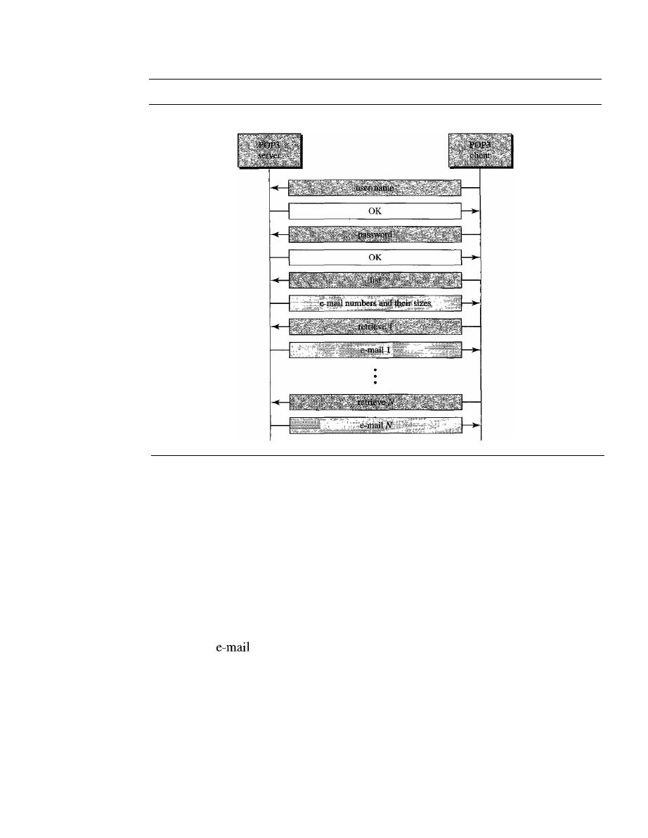
SECTION
26.2
ELECTRONIC MAIL
839
Figure 26.20
The exchange of commands and responses in POP3
Mail server
Bob's computer
POP3 is deficient in several ways. It does not allow the user to organize her mail on
the server; the user cannot have different folders on the server. (Of course, the user can
create folders on her own computer.) In addition, POP3 does not allow the user to
partially check the contents of the mail before downloading.
IMAP4 provides the following extra functions:
o
A user can check the e-mail header prior to downloading.
o
A user can search the contents of the e-mail for a specific string of characters prior
to downloading.
o
A user can partially download e-mail. This is especially useful if bandwidth is limited
and the
contains multimedia with high bandwidth requirements.
o
A user can create, delete, or rename mailboxes on the mail server.
o
A user can create a hierarchy of mailboxes in a folder for e-mail storage.
Web-Based Mail
E-mail is such a common application that some websites today provide this service to
anyone who accesses the site. Two common sites are Hotmail and Yahoo. The idea is very
simple. Mail transfer from Alice's browser to her mail server is done through HTTP (see
Chapter 27). The transfer of the message from the sending mail server to the receiving

840
CHAPTER
26
REMOTE LOGGING, ELECTRONIC MAIL, AND FILE TRANSFER
mail server is still through SMTP. Finally, the message from the receiving server (the Web
server) to Bob's browser is done through HTIP.
The last phase is very interesting. Instead of POP3 or IMAP4, HTTP is normally
used. When Bob needs to retrieve his e-mails, he sends a message to the website (Hotmail,
for example). The website sends a form to be filled in by Bob, which includes the log-in
name and the password.
If
the log-in name and password match, the e-mail is transferred
from the Web server to Bob's browser in HTML format.
26.3
FILE TRANSFER
Transferring files from one computer to another is one of the most common tasks
expected from a networking or internetworking environment. As a matter of fact, the
greatest volume of data exchange in the Internet today is due to file transfer. In this
section, we discuss one popular protocol involved in transferring files: File Transfer
Protocol
(FTP).
File Transfer Protocol (FTP)
File Transfer Protocol (FTP) is the standard mechanism provided by
TCP/IP
for
copying a file from one host to another. Although transferring files from one system to
another seems simple and straightforward, some problems must be dealt with first. For
example, two systems may use different file name conventions. Two systems may have
different ways to represent text and data. Two systems may have different directory
structures. All these problems have been solved by FTP in a very simple and elegant
approach.
FTP differs from other client/server applications in that it establishes two connec-
tions between the hosts. One connection is used for data transfer, the other for control
information (commands and responses). Separation of commands and data transfer
makes FTP more efficient. The control connection uses very simple rules of communi-
cation. Wc need to transfer only a line of command or a line of response at a time. The
data connection, on the other hand, needs more complex rules due to the variety of data
types transferred. However, the difference in complexity is at the FTP level, not TCP.
For TCP, both connections are treated the same.
FTP uses two well-known TCP ports: Port 21 is used for the control connection,
and port 20 is used for the data connection.
FTP uses the services of TCP.
It
needs two TCP connections.
The well-known port 21 is used for the control connection
and the well-known port 20 for the data connection.
Figure 26.21 shows the basic model of FTP. The client has three components: user
interface, client control process, and the client data transfer process. The server has two
components: the server control process and the server data transfer process. The control
connection is made between the control processes. The data connection is made between
the data transfer processes.
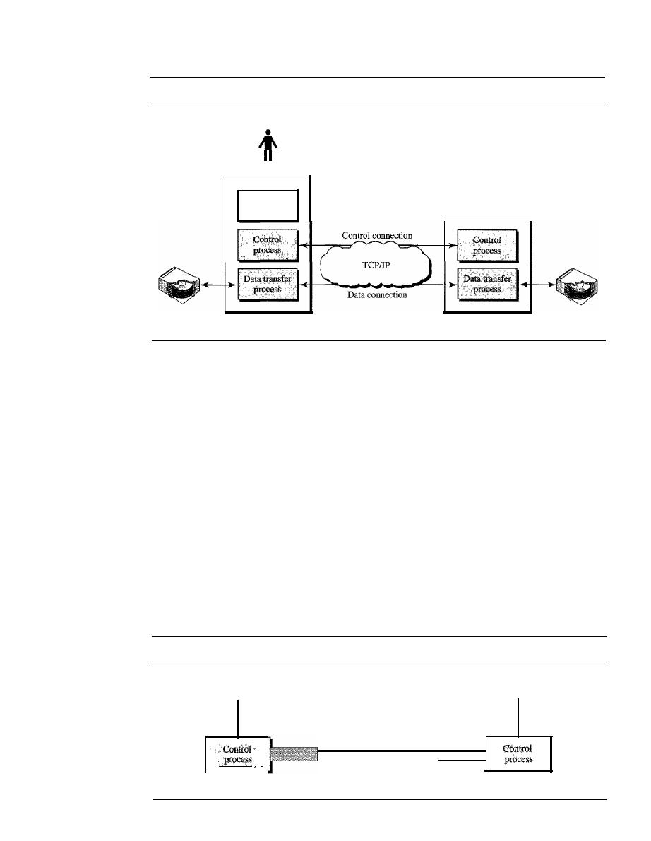
SECTION
26.3
FILE TRANSFER
841
Figure 26.21
FTP
User
User
interface
Client
Server
The control connection remains connected during the entire interactive FTP ses-
sion. The data connection is opened and then closed for each file transferred.
It
opens
each time commands that involve transferring files are used, and it closes when the file
is transferred. In other words, when a user starts an FTP session, the control connection
opens. While the control connection is open, the data connection can be opened and
closed multiple times if several files are transferred.
Communication over Control Connection
FTP uses the same approach as SMTP to communicate across the control connection.
It
uses the 7-bit ASCII character set (see Figure 26.22). Communication is achieved
through commands and responses. This simple method is adequate for the control con-
nection because we send one command (or response) at a time. Each command or
response is only one short line, so we need not worry about file format or file structure.
Each line is terminated with a two-character (carriage return and line feed) end-of-line
token.
Figure 26.22
Using the control connection
Local
code
,
,
'
Client
NVTASCII
Control
connection
Local
code
"
"
'
Server
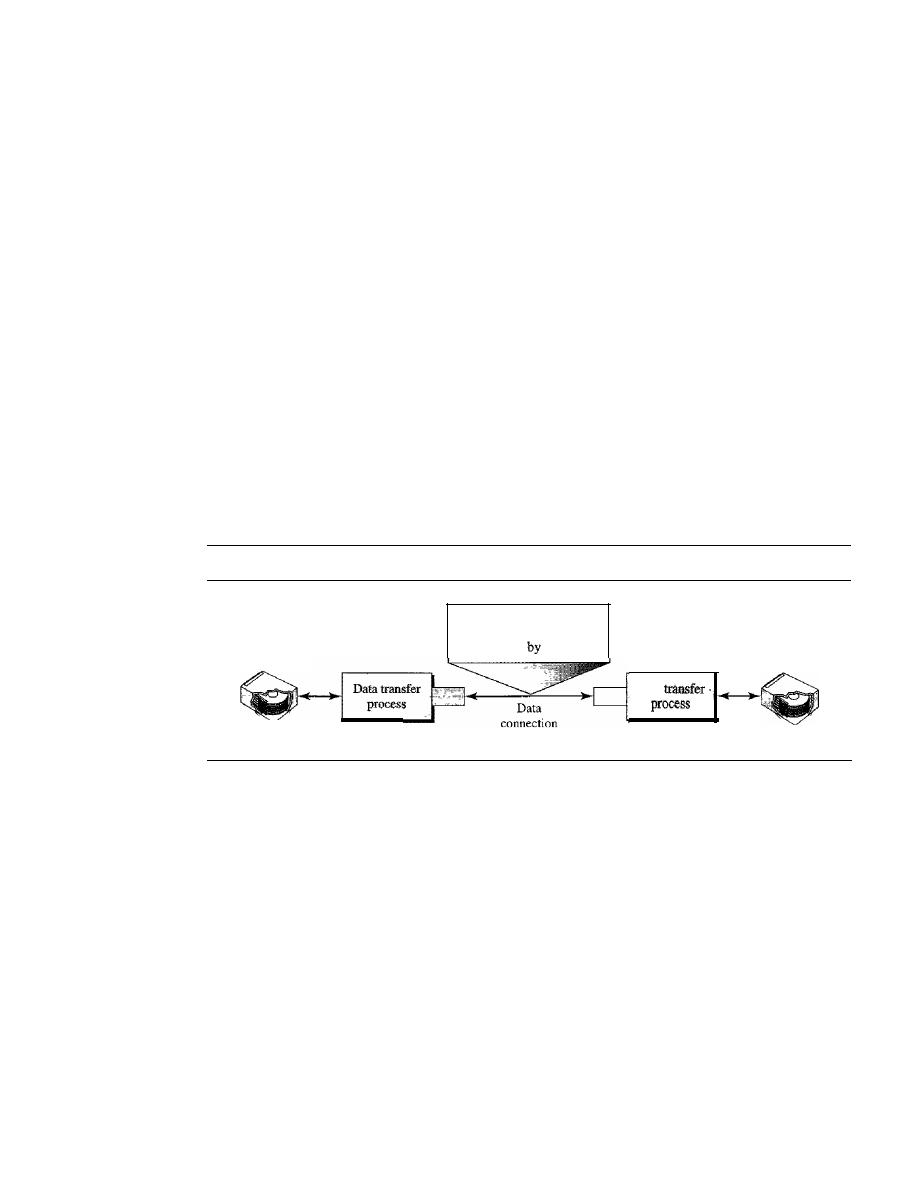
842
CHAPTER
26
REMOTE LOGGING, ELECTRONIC MAIL, AND FILE TRANSFER
Communication over Data Connection
The purpose of the data connection is different from that of the control connection. We
want to transfer files through the data connection. File transfer occurs over the data
connection under the control of the commands sent over the control connection. How-
ever, we should remember that file transfer in FTP means one of three things:
o
A file is to be copied from the server to the client. This is called
retrieving aft/e.
It
is done under the supervision of the RETR command,
o
A file is to be copied from the client to the server. This is called
storing aft/e.
It
is
done under the supervision of the STOR command.
o
A list of directory or file names is to be sent from the server to the client. This is
done under the supervision of the LIST command. Note that FTP treats a list of
directory or file names as a file.
It
is sent over the data connection.
The client must define the type of file to be transferred, the structure of the data,
and the transmission mode. Before sending the file through the data connection, we
prepare for transmission through the control connection. The heterogeneity problem is
resolved by defining three attributes of communication: file type, data structure, and
transmission mode (see Figure 26.23).
Figure 26.23
Using the data connection
Local data type
and structure
Client
File type, data structure,
and transmission mode
are defined
the client
Local data type
and structure
Data
Server
File Type
FTP can transfer one of the following file types across the data connection:
an ASCII file, EBCDIC file, or image file. The
ASCII file
is the default format for trans-
ferring text files. Each character is encoded using 7-bit ASCII. The sender transforms
the file from its own representation into ASCII characters, and the receiver transforms
the ASCII characters to its own representation. If one or both ends of the connection
use EBCDIC encoding (the file format used by IBM), the file can be transferred using
EBCDIC encoding. The
image file
is the default format for transferring binary files.
The file is sent as continuous streams of bits without any interpretation or encoding.
This is mostly used to transfer binary files such as compiled programs.
Data Structure
FTP can transfer a file across the data connection by using one of the
following interpretations about the structure of the data: file structure, record structure,
and page structure. In the
file structure
format, the file is a continuous stream of bytes. In
the
record structure,
the file is divided into records. This can be used only with text files.
In
the
page structure,
the file is divided into pages, with each page having a page number
and a page header. The pages can be stored and accessed randomly or sequentially.

SECTION
26.3
FILE TRANSFER
843
Transmission Mode
FTP can transfer a file across the data connection by using one
of the following three transmission modes: stream mode, block mode, and compressed
mode. The
stream mode
is the default mode. Data are delivered from FTP to TCP as a
continuous stream of bytes. TCP is responsible for chopping data into segments of
appropriate size.
If
the data are simply a stream of bytes (file structure), no end-of-file
is needed. End-of-file in this case is the closing of the data connection by the sender.
If
the data are divided into records (record structure), each record will have a I-byte end-
of-record (EOR) character and the end of the file will have a I-byte end-of-file (EOF)
character. In
block mode,
data can be delivered from FTP to TCP in blocks. In this
case, each block is preceded by a 3-byte header. The first byte is called the block
descriptor; the next 2 bytes define the size of the block in bytes. In the
compressed
mode,
if the file is big, the data can be compressed. The compression method normally
used is run-length encoding. In this method, consecutive appearances of a data unit are
replaced by one occurrence and the number of repetitions. In a text file, this is usually
spaces (blanks). In a binary file, null characters are usually compressed.
Example 26.4
The following shows an actual
FTP
session for retrieving a list of items in a directory. The col-
ored lines show the responses from the server control connection; the black lines show the com-
mands sent by the client. The lines in white with a black background show data transfer.
$ ftp voyager.deanza.tbda.edu
Connected to voyager.deanza.tbda.edu.
220
(vsFTPd
1.2.1)
530
Please login with USER and PASS.
Name (voyager.deanza.tbda.edu:forouzan): forouzan
331
Please specify the password.
Password:
230
Login successful.
Remote system type is UNIX.
Using binary mode to transfer files.
ftp> Is reports
227
Entering Passive Mode
(153,18,17,11,238,169)
150
Here comes the directory listing.
drwxr-xr-x
23027
411
4096 Sep 24 2002 business
drwxr-xr-x
23027
411
4096 Sep 24 2002 personal
drwxr-xr-x
23027
411
4096 Sep 24 2002 school
226
Directory send
OK.
ftp>quit
221 Goodbye.
1. After the control connection is created, the FIP server sends the 220 (service ready) response
on the control connection.
2. The client sends its name.
3. The server responds with 331 (user name is OK, password
required).
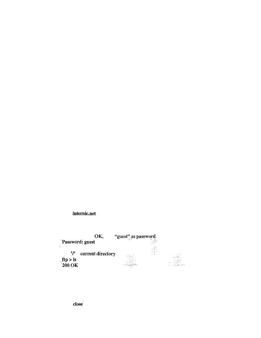
844
CHAPTER
26
REMOTE LOGGING, ELECTRONIC MAIL, AND FILE TRANSFER
4. The client sends the password (not shown).
5. The server responds with 230 (user log-in is OK).
6. The client sends the list command Os reports) to find the list of files on the directory named
report.
7. Now the server responds with 150 and opens the data connection.
8. The server then sends the list of the files or directories (as a file) on the data connection.
When the whole list (file) is sent, the server responds with 226 (closing data connection)
over the control connection.
9. The client now has two choices. It can use the QUIT command to request the closing of the
control connection, or it can send another command to start another activity (and eventually
open another data connection). In our example, the client sends a QUIT command.
10. After receiving the QUIT command, the server responds with 221 (service closing) and then
closes the control connection.
Anonymous FTP
To use FfP, a user needs an account (user name) and a password on the remote server.
Some sites have a set of files available for public access, to enable anonymous
FTP.
To
access these files, a user does not need to have an account or password. Instead, the user
can use anonymous as the user name and guest as the password.
User access to the system is very limited. Some sites allow anonymous users only
a subset of commands. For example, most sites allow the user to copy some files, but do
not allow navigation through the directories.
Example 26.5
We show an example of anonymous FTP. We assume that some public data are available at
intemic.net.
$
ftp
Connected to internic.net
220 Server ready
Name: anonymous
331 Guest login
send
ftp>pwd"
257
is
150 Opening ASCII mode
bin
...
ttp>
221 Goodbye
ftp>quit
SECTION
26.5
KEY TERMS
845
26.4
RECOMMENDED READING
For more details about subjects discussed in this chapter, we recommend the following
books and sites. The items in brackets [...] refer to the reference list at the end of the text.
Books
Remote logging is discussed in Chapter 18 of [For06] and Chapter 26 of [Ste94].
Electronic mail is discussed in Chapter 20 of [For06], Section 9.2 of [PD03], Chapter 32
of [Com04], Section 7.2 of [Tan03], and Chapter 28 of [Ste94]. FTP is discussed in
Chapter 19 of [For06], Chapter 27 of [Ste94], and Chapter 34 of [Com04].
Sites
The following sites are related to topics discussed in this chapter.
o
www.ietf.org/rfc.htrnl
Information about RFCs
RFCs
The following RFCs are related to TELNET:
The following RFCs are related to SMTP, POP, and IMAP:
The following RFCs are related to FTP:
;
DNS is discussed in [AL98], chapter 17 of [For06], section 9.1 of [PD03], and
section 7.1 of [Tan03].
26.5
KEY TERMS
alias
anonymous FTP
ASCII file
block mode
body
character mode
compressed mode
control character
control connection
data connection

846
CHAPTER
26
REMOTE LOGGING, ELECTRONIC MAIL, AND FILE TRANSFER
default mode
domain name
envelope
file structure
File Transfer Protocol (FTP)
header
image file
Internet Mail Access Protocol, version 4
(IMAP4)
line mode
local log-in
local part
message access agent (MAA)
message transfer agent (MTA)
Multipurpose Internet Mail Extensions
(MIME)
network virtual terminal (NVT)
option negotiation
page structure
Post Office Protocol, version 3 (POP3)
record structure
remote log-in
Simple Mail Transfer Protocol (SMTP)
stream mode
suboption negotiation
terminal network (TELNET)
timesharing
user agent
(VA)
26.6
SUMMARY
o
TELNET is a client/server application that allows a user to log on to a remote
machine, giving the user access to the remote system.
o
TELNET uses the network virtual terminal (NVT) system to encode characters on
the local system. On the server machine, NVT decodes the characters to a form
acceptable to the remote machine.
o
NVT uses a set of characters for data and a set of characters for control.
o
In TELNET, control characters are embedded in the data stream and preceded by
the interpret as control (lAC) control character.
D
Options are features that enhance the TELNET process.
o
TELNET allows negotiation to set transfer conditions between the client and server
before and during the use of the service.
D
A TELNET implementation operates in the default, character, or line mode.
1. In the default mode, the client sends one line at a time to the server.
2. In the character mode, the client sends one character at a time to the server.
3. In the line mode, the client sends one line at a time to the server.
D
Several programs, including SMTP, POP3, and IMAP4, are used in the Internet to
provide electronic mail services.
D
In electronic mail, the
VA
prepares the message, creates the envelope, and puts the
message in the envelope.
D
In electronic mail, the mail address consists of two parts: a local part (user mailbox)
and a domain name. The form is localpart@domainname.
o
In electronic mail, Multipurpose Internet Mail Extension (MIME) allows the transfer
of multimedia messages.
o
In electronic mail, the MTA transfers the mail across the Internet, a LAN, or a WAN.

SECTION
26. 7
PRACTICE SET
847
o
SMTP uses commands and responses to transfer messages between an MTA client
and an MTA server.
o
The steps in transferring a mail message are
1. Connection establishment·
2. Mail transfer
3. Connection termination
o
Post Office Protocol, version 3 (POP3) and Internet Mail Access Protocol, version 4
(IMAP4) are protocols used for pulling messages from a mail server.
o
One of the programs used for file transfer in the Internet is File Transfer Protocol
(FTP).
o
FTP requires two connections for data transfer: a control connection and a data
connection.
o
FTP employs NVT ASCII for communication between dissimilar systems.
o
Prior to the actual transfer of files, the file type, data structure, and transmission
mode are defined by the client through the control connection.
o
Responses are sent from the server to the client during connection establishment.
o
There are three types of file transfer:
1. A file is copied from the server to the client.
2. A file is copied from the client to the server.
3. A list of directories or file names is sent from the server to the client.
o
Anonymous FTP provides a method for the general public to access files on remote
sites.
26.7
PRACTICE SET
Review Questions
1. What is the difference between local and remote log-in in TELNET?
2. How are control and data characters distinguished in NVT?
3. How are options negotiated in TELNET?
4. Describe the addressing system used by SMTP.
5. In electronic mail, what are the tasks of a user agent?
6. In electronic mail, what is MIME?
7. Why do we need POP3 or IMAP4 for electronic mail?
8. What is the purpose of FTP?
9. Describe the functions of the two FTP connections.
10. What kinds of file types can FTP transfer?
11. What are the three FTP transmission modes?
12. How does storing a file differ from retrieving a file?
13. What is anonymous FTP?

848
CHAPTER
26
REMOTE LOGGING, ELECTRONIC MAIL, AND FILE TRANSFER
Exercises
14. Show the sequence of bits sent from a client TELNET for the binary transmission
of11110011 00111100 11111111.
15.
If
TELNET is using the character mode, how many characters are sent back and
forth between the client and server to copy a file named file
1
to another file named
file2 using the command
cp file 1 file2?
16. What is the minimum number of bits sent at the TCP level to accomplish the task
in Exercise
IS?
17. What is the minimum number of bits sent at the data link layer level (using Ethernet)
to accomplish the task in Exercise 15?
18. What is the ratio of the useful bits to the total bits in Exercise 17?
19. Interpret the following sequences of characters (in hexadecimal) received by a
TELNET client or server.
a.
FFFB 01
b. FFFEOI
c.
FFF4
d. FFF9
20. A sender sends unformatted text. Show the MIME header.
21. A sender sends a IPEG message. Show the MIME header.
22. Why is a connection establishment for mail transfer needed if TCP has already
established a connection?
23. Why should there be limitations on anonymous FTP? What could an unscrupulous
user do?
24. Explain why FTP does not have a message format.
Research Activities
25. Show the sequence of characters exchanged between the TELNET client and the
server to switch from the default mode to the character mode.
26. Show the sequence of characters exchanged between the TELNET client and the
server to switch from the default mode to line mode.
27. In SMTP, show the connection establishment phase from aaa@xxx.com to
bbb@yyy.com.
28. In SMTP, show the message transfer phase from aaa@xxx.com to bbb@yyy.com.
The message is "Good morning my friend."
29. In SMTP, show the connection termination phase from aaa@xxx.com to
bbb@yyy.com.
30. What do you think would happen if the control connection were accidentally severed
during an FTP transfer?

SECTION
26. 7
PRACTICE SET
849
31. Find the extended options proposed for TELNET.
32. Another log-in protocol is called Rlogin. Find some information about Rlogin and
compare it with TELNET.
33. A more secure log-in protocol in UNIX is called Secure Shell (SSH). Find some
information about this protocol.

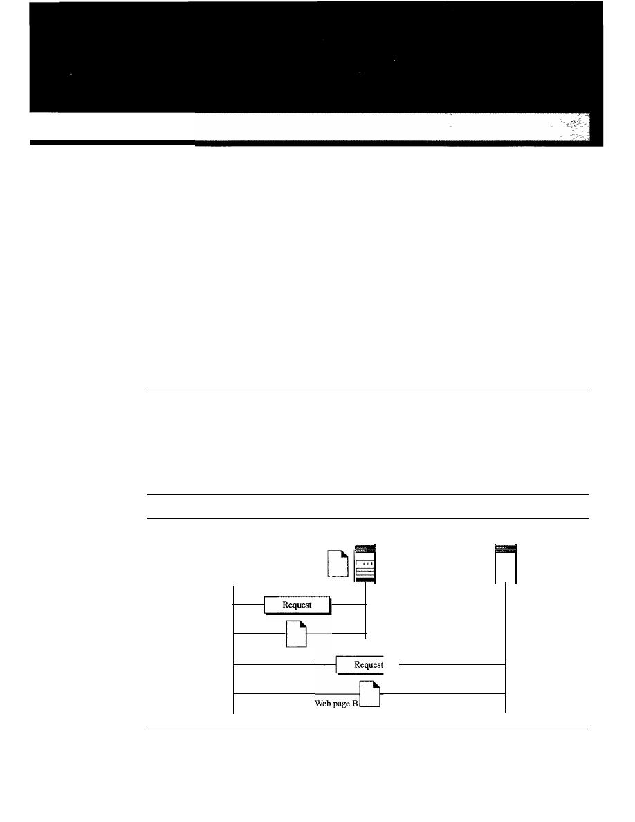
CHAPTER 27
WWWandHTTP
The World Wide Web (WWW) is a repository of information linked together from
points all over the world. The WWW has a unique combination of flexibility, portability,
and user-friendly features that distinguish it from other services provided by the Internet.
The WWW project was initiated by CERN (European Laboratory for Particle Physics)
to create a system to handle distributed resources necessary for scientific research.
In
this chapter we first discuss issues related to the Web. We then discuss a protocol,
HTTP, that is used to retrieve information from the Web.
27.1
ARCHITECTURE
The WWW today is a distributed clientJserver service, in which a client using a browser
can access a service using a server. However, the service provided is distributed over
many locations called sites, as shown
in
Figure 27.1.
Figure 27.1
Architecture ofWWW
Client
Web page A
Site A
D
Site
B
851
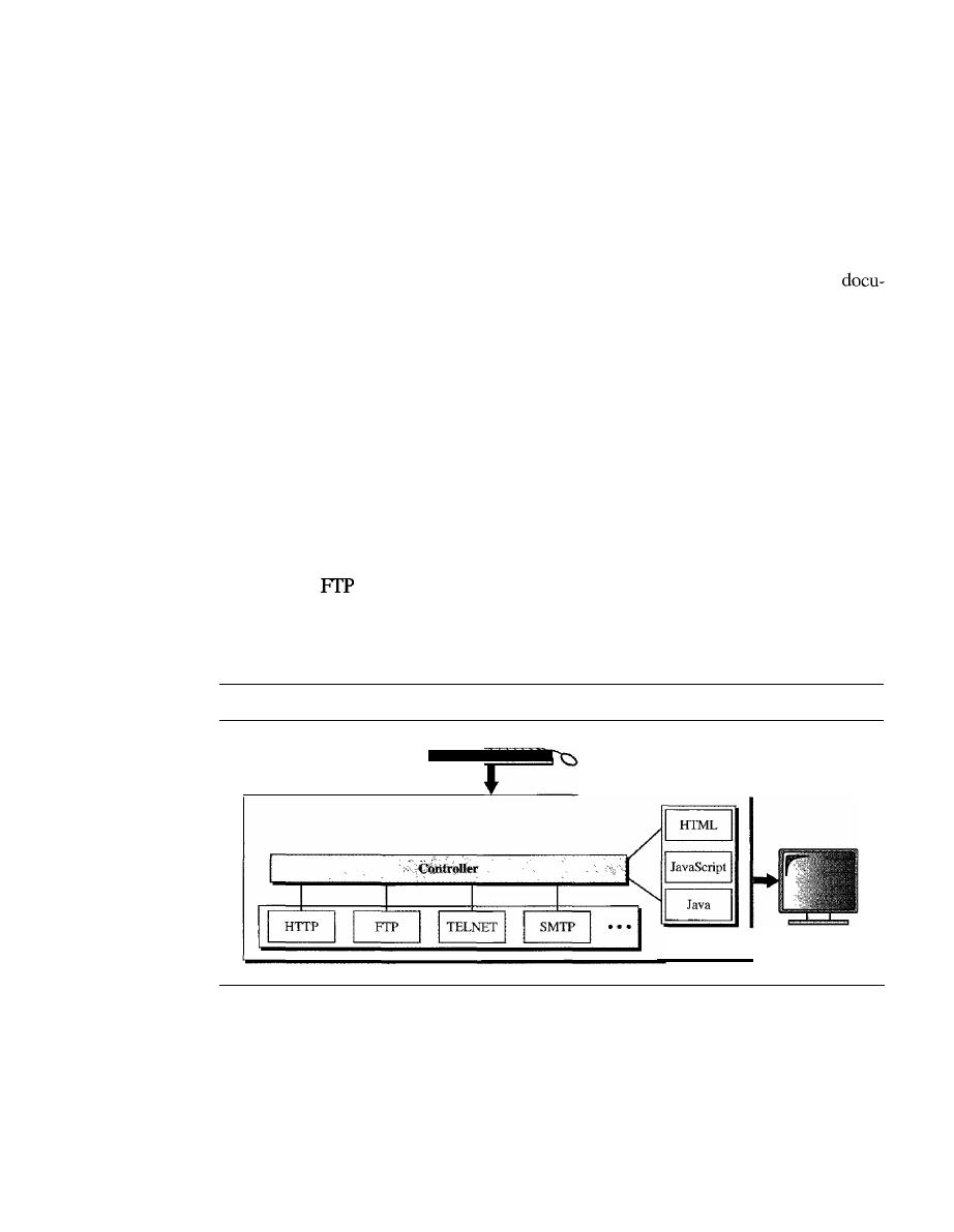
852
CHAPTER
27
WWW AND HTTP
Each site holds one or more documents, referred to as Web pages. Each Web page can
contain a link to other pages in the same site or at other sites. The pages can be retrieved
and viewed by using browsers. Let us go through the scenario shown in Figure 27.1. The
client needs to see some information that it knows belongs to site A. It sends a request
through its browser, a program that is designed to fetch Web documents. The request,
among other information, includes the address of the site and the Web page, called the
URL, which we will discuss shortly. The server at site A finds the document and sends it
to the client. When the user views the document, she finds some references to other
ments, including a Web page at site B. The reference has the URL for the new site. The
user is also interested in seeing this document. The client sends another request to the new
site, and the new page is retrieved.
Client (Browser)
A variety of vendors offer commercial browsers that interpret and display a Web docu-
ment, and all use nearly the same architecture. Each browser usually consists of three
parts: a controller, client protocol, and interpreters. The controller receives input from
the keyboard or the mouse and uses the client programs to access the document. After
the document has been accessed, the controller uses one of the interpreters to display the
document on the screen. The client protocol can be one of the protocols described previ-
ously such as
or HTIP (described later in the chapter). The interpreter can be HTML,
J
ava, or JavaScript, depending on the type of document. We discuss the use of these
interpreters based on the document type later in the chapter (see Figure 27.2).
Figure 27.2
Browser
Browser
Interpreters
Server
The Web page is stored at the server. Each time a client request arrives, the corresponding
document is sent to the client. To improve efficiency, servers normally store requested
files in a cache in memory; memory is faster to access than disk. A server can also
become more efficient through multithreading or multiprocessing. In this case, a server
can answer more than one request at a time.
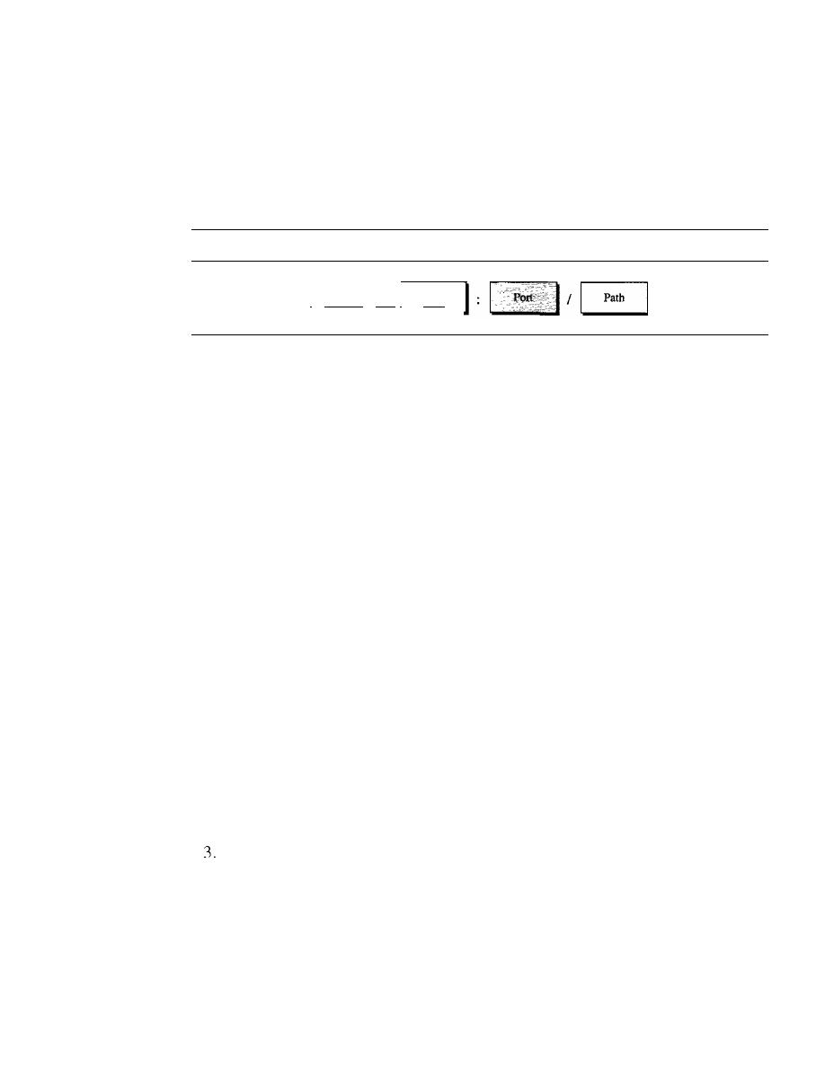
SECTION
27.1
ARCHITECTURE
853
Uniform Resource Locator
A client that wants to access a Web page needs the address. To facilitate the access of doc-
uments distributed throughout the world, HTTP uses locators. The
uniform resource
locator
(URL) is a standard for specifying any kind of information on the Internet. The
URL defines four things: protocol, host computer, port, and path (see Figure 27.3).
Figure 27.3
URL
I
Protocol
1://
I
Host
The protocol is the client/server program used to retrieve the document. Many
different protocols can retrieve a document; among them are FTP or HTTP. The most
common today is HTTP.
The
host
is the computer on which the information is located, although the name of
the computer can be an alias. Web pages are usually stored in computers, and computers
are given alias names that usually begin with the characters "www". This is not mandatory,
however, as the host can be any name given to the computer that hosts the Web page.
The URL can optionally contain the port number of the server.
If
the port is
included, it is inserted between the host and the path, and it is separated from the host
by a colon.
Path
is the pathname of the file where the information is located. Note that the path
can itself contain slashes that, in the UNIX operating system, separate the directories
from the subdirectories and files.
Cookies
The World Wide Web was originally designed as a stateless entity. A client sends a
request; a server responds. Their relationship is over. The original design of WWW,
retrieving publicly available documents, exactly fits this purpose. Today the Web has
other functions; some are listed here.
I.
Some websites need to allow access to registered clients only.
2. Websites are being used as electronic stores that allow users to browse through the
store, select wanted items, put them in an electronic cart, and pay at the end with a
credit card.
Some websites are used as portals: the user selects the Web pages he wants to see.
4. Some websites are just advertising.
For these purposes, the cookie mechanism was devised. We discussed the use of cook-
ies at the transport layer in Chapter 23; we now discuss their use in Web pages.
Creation and Storage of Cookies
The creation and storage of cookies depend on the implementation; however, the principle
is the same.

854
CHAPTER
27
WWW
AND HTTP
1. When a server receives a request from a client, it stores information about the client
in a file or a string. The information may include the domain name of the client, the
contents of the cookie (information the server has gathered about the client such as
name, registration number, and so on), a timestamp, and other information'depend-
ing on the implementation.
2. The server includes the cookie in the response that it sends to the client.
3. When the client receives the response, the browser stores the cookie in the cookie
directory, which is sorted by the domain server name.
Using Cookies
When a client sends a request to a server, the browser looks in the cookie directory to
see if it can find a cookie sent by that server.
If
found, the cookie is included in the
request. When the server receives the request, it knows that this is an old client, not a
new one. Note that the contents of the cookie are never read by the browser or disclosed
to the user.
It
is a cookie
made by the server and eaten by the server. Now let us see how
a cookie is used for the four previously mentioned purposes:
1. The site that restricts access to registered clients only sends a cookie to the client
when the client registers for the first time. For any repeated access, only those clients
that send the appropriate cookie are allowed.
2. An electronic store (e-commerce) can use a cookie for its client shoppers. When a
client selects an item and inserts it into a cart, a cookie that contains information
about the item, such as its number and unit price, is sent to the browser. If the client
selects a second item, the cookie is updated with the new selection information. And
so on. When the client finishes shopping and wants to check out, the last cookie is
retrieved and the total charge is calculated.
3. A Web portal uses the cookie in a similar way. When a user selects her favorite
pages, a cookie is made and sent.
If
the site is accessed again, the cookie is sent to
the server to show what the client is looking for.
4. A cookie is also used by advertising agencies.
An
advertising agency can place
banner ads on some main website that is often visited by users. The advertising
agency supplies only a URL that gives the banner address instead of the banner itself.
When a user visits the main website and clicks on the icon of an advertised corpora-
tion, a request is sent to the advertising agency. The advertising agency sends the
banner, a GIF file, for example, but it also includes a cookie with the
ill
of the user.
Any future use of the banners adds to the database that profiles the Web behavior of
the user. The advertising agency has compiled the interests of the user and can sell
this information to other parties. This use of cookies has made them very controver-
sial. Hopefully, some new regulations will be devised to preserve the privacy of users.
27.2
WEB DOCUMENTS
The documents in the WWW can be grouped into three broad categories: static, dynamic,
and active. The category is based on the time at which the contents of the document are
determined.
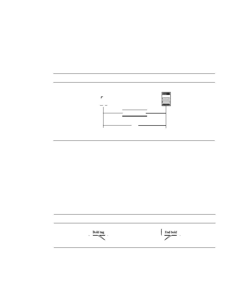
SECTION
27.2
WEB DOCUMENTS
855
Static Documents
Static documents
are fixed-content documents that are created and stored in a server.
The client can get only a copy of the document. In other words, the contents of the file
are determined when the file is created, not when it is used. Of course, the contents in
the server can be changed, but the user cannot change them. When a client accesses the
document, a copy of the document is sent. The user can then use a browsing program to
display the document (see Figure 27.4).
Figure 27.4
Static document
Server
Client
-
-
Request
Static HTML document
HTML
Hypertext Markup Language (HTML)
is a language for creating Web pages. The
term markup language comes from the book publishing industry. Before a book is type-
set and printed, a copy editor reads the manuscript and puts marks on it. These marks
tell the compositor how to format the text. For example, if the copy editor wants part of
a line to be printed in boldface, he or she draws a wavy line under that part. In the same
way, data for a Web page are formatted for interpretation by a browser.
Let us clarify the idea with an example. To make part of a text displayed in boldface
with HTML, we put beginning and ending boldface
tags
(marks) in the text, as shown
in Figure 27.5.
Figure 27.5
Boldface tags
I
1
]
<B> This is the text to be boldfaced.<!B>
The two tags <B> and </B> are instructions for the browser. When the browser
sees these two marks, it knows that the text must be boldfaced (see Figure 27.6).
A markup language such as HTML allows us to embed formatting instructions in
the file itself. The instructions are included with the text. In this way, any browser can
read the instructions and format the text according to the specific workstation. One might
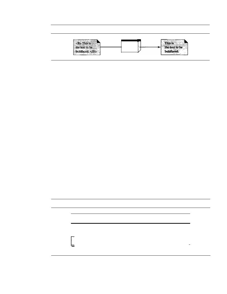
856
CHAPTER
27
WWW AND HTTP
Figure 27.6
Effect of boldface tags
Browser
ask why we do not use the fonnatting capabilities of word processors to create and save
formatted text. The answer is that different word processors use different techniques or
procedures for formatting text. For example, imagine that a user creates formatted text on
a Macintosh computer and stores it in a Web page. Another user who is on an IBM com-
puter would not be able to receive the Web page because the two computers use different
fonnatting procedures.
HTML lets us use only ASCII characters for both the main text and formatting
instructions. In this way, every computer can receive the whole document as an ASCII
document. The main text is the data, and the formatting instructions can be used by the
browser to format the data.
A Web page is made up of two parts: the head and the body. The head is the first part
of a Web page. The head contains the title of the page and other parameters that the
browser will use. The actual contents of a page are in the body, which includes the text and
the tags. Whereas the text is the actual infonnation contained in a page, the tags define the
appearance of the document. Every HTML tag is a name followed by an optional list of
attributes, all enclosed between less-than and greater-than symbols
«
and
>).
An attribute, if present, is followed by an equals sign and the value of the attribute.
Some tags can be used alone; others must be used in pairs. Those that are used in pairs
are called beginning and ending tags. The beginning tag can have attributes and values
and starts with the name of the tag. The ending tag cannot have attributes or values but
must have a slash before the name of the tag. The browser makes a decision about the
structure of the text based on the tags, which are embedded into the text. Figure 27.7
shows the fonnat of a tag.
Figure 27.7
Beginning and ending tags
<
TagNarne
a. Beginning tag
Attribute
=
Value
Attribute
=
Value
••• >
<_rr_a_gN_arn_e_>
1
b. Ending tag
One commonly used tag category is the text formatting tags such as <B> and
<!B>,
which make the text bold; <1> and <II>, which make the text italic; and <U> and
<IV>,
which underline the text.
SECTION
27.2
WEB DOCUMENTS
857
Another interesting tag category is the image tag. Nontextual information such as
digitized photos or graphic images is not a physical part of an HTML document. But
we can use an image tag to point to the file of a photo or image. The image tag defines
the address (URL) of the image to be retrieved.
It
also specifies how the image can be
inserted after retrievaL We can choose from several attributes. The most common are
SRC (source), which defines the source (address), and ALIGN, which defines the align-
ment of the image. The SRC attribute is required. Most browsers accept images in the
GIF or IPEG formats. For example, the following tag can retrieve an image stored as
imagel.gif in the directory /bin/images:
A third interesting category is the hyperlink tag, which is needed to link documents
together. Any item (word, phrase, paragraph, or image) can refer to another document
through a mechanism called an anchor. The anchor is defined by <A ... > and
<!
A> tags,
and the anchored item uses the URL to refer
to
another document. When the document
is displayed, the anchored item is underlined, blinking, or boldfaced. The user can click
on the anchored item to go to another document, which mayor may not be stored on
the same server as the original document. The reference phrase is embedded between the
beginning and ending tags. The beginning tag can have several attributes, but the one
required is HREF (hyperlink reference), which defines the address (URL) of the linked
document. For example, the link to the author of a book can be
What appears in the text is the word Author, on which the user can click to go to the
author's Web page.
Dynamic Documents
A
dynamic document
is created by a Web server whenever a browser requests the doc-
ument. When a request arrives, the Web server runs an application program or a script
that creates the dynamic document. The server returns the output of the program or
script as a response to the browser that requested the document. Because a fresh docu-
ment is created for each request, the contents of a dynamic document can vary from
one request to another. A very simple example of a dynamic document is the retrieval
of the time and date from a server. Time and date are kinds of information that are
dynamic in that they change from moment to moment. The client can ask the server to
run a program such as the date program in UNIX and send the result of the program to
the client.
Common Gateway Interface (CGI)
The
Common
Gateway Interface (CGI)
is a technology that creates and handles
dynamic documents. CGI is a set of standards that defines how a dynamic document is
written, how data are input to the program, and how the output result is used.
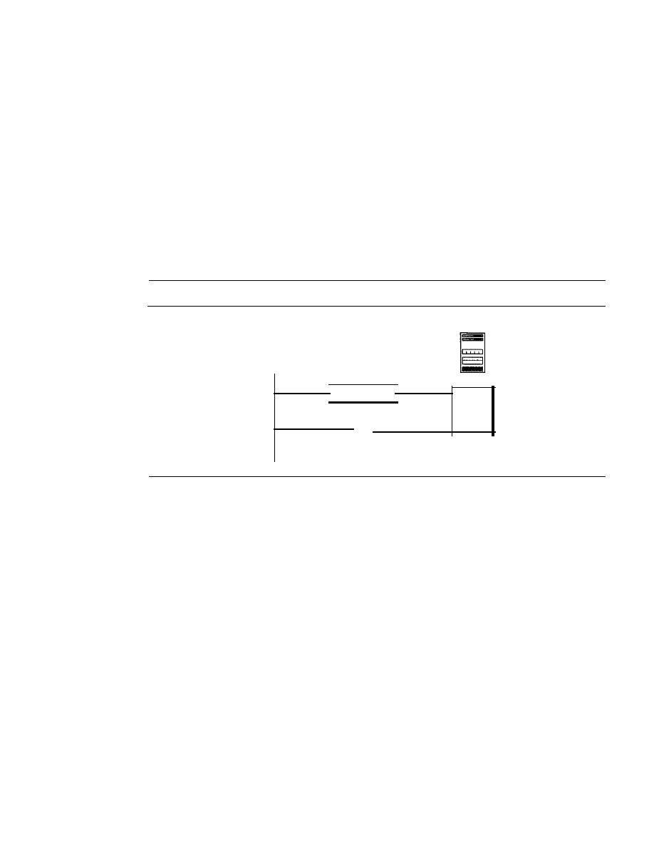
858
CHAPTER
27
WWW AND HTTP
COl is not a new language; instead, it allows programmers to use any of several
languages such as C, C++, Boume Shell, Kom Shell, C Shell, Tcl, or Perl. The only
thing that CGI defines is a set of rules and tenns that the programmer must follow.
The tenn common in COl indicates that the standard defines a set of rules that is
common to any language or platfonn. The tenn gateway here means that a COl pro-
gram can be used to access other resources such as databases, graphical packages, and
so on. The tenn interface here means that there is a set of predefined tenns, variables,
calls, and so on that can be used in any COl program. A COl program in its simplest
fonn is code written in one of the languages supporting COL Any programmer who can
encode a sequence of thoughts in a program and knows the syntax of one of the above-
mentioned languages can write a simple CGI program. Figure 27.8 illustrates the steps
in creating a dynamic program using COl technology.
Figure 27.8
Dynamic document using CGI
Client
Request
Dynamic HTML document
Server
Program
Input
In traditional programming, when a program is executed, parameters can be
passed to the program. Parameter passing allows the programmer to write a generic
program that can be used in different situations. For example, a generic copy program
can be written to copy any file to another. A user can use the program to copy a file
named x to another file named y by passing x and y as parameters.
The input from a browser to a server is sent by using aform.
If
the infonnation in a
fonn is small (such as a word), it can be appended to the URL after a question mark. For
example, the following URL is carrying fonn infonnation (23, a value):
http://www.deanzalcgi-binlprog.pl?23
When the server receives the URL, it uses the part of the URL before the question
mark to access the program to be run, and it interprets the part after the question mark
(23) as the input sent by the client.
It
stores this string in a variable. When the CGI
program is executed, it can access this value.
If the input from a browser is too long to fit in the query string, the browser can ask
the server to send a fonn. The browser can then fill the fonn with the input data and
send it to the server. The infonnation in the fonn can be used as the input to the COl
program.
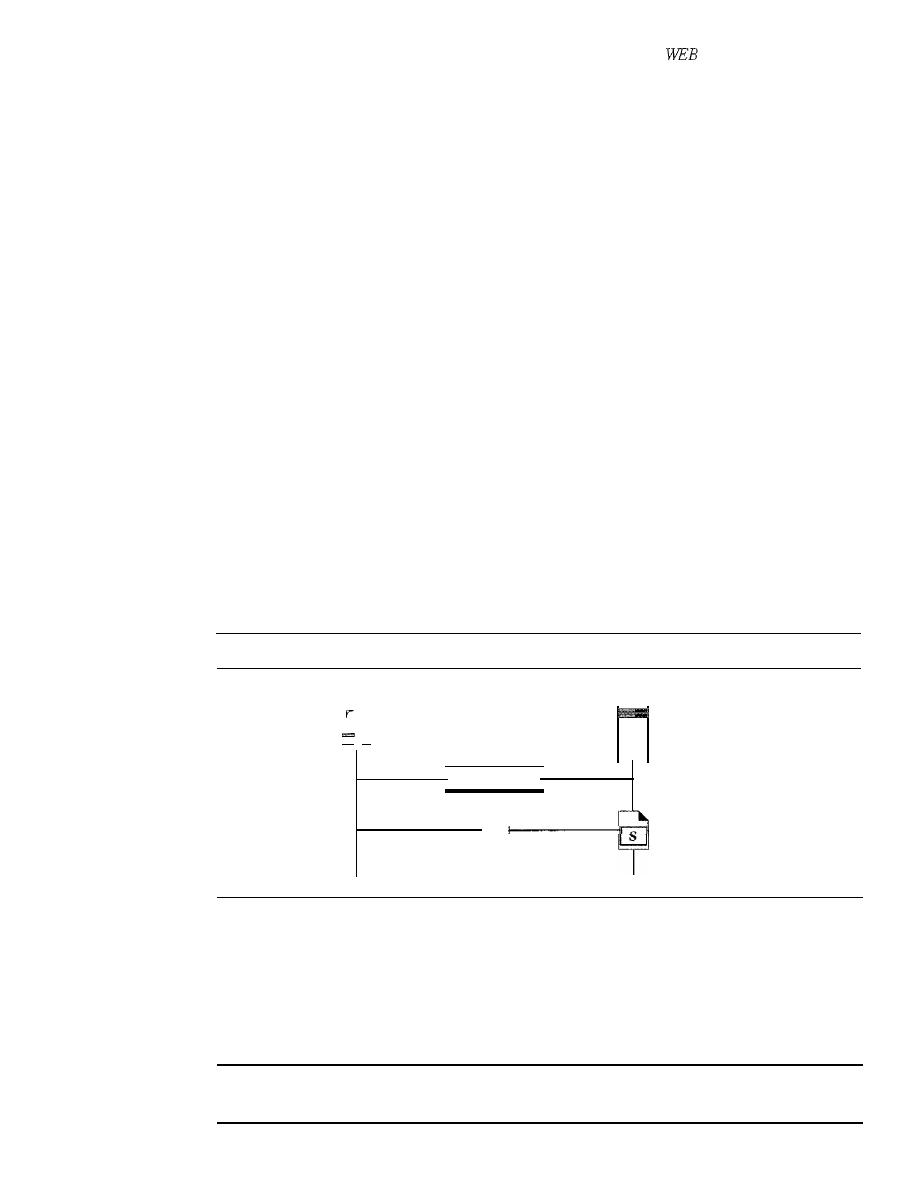
SECTION 27.2
DOCUMENTS
859
Output
The whole idea of CGI is to execute a CGI program at the server site and
send the output to the client (browser). The output is usually plain text or a text with
HTML structures; however, the output can be a variety of other things.
It
can be graphics
or binary data, a status code, instructions to the browser to cache the result, or instruc-
tions to the server to send an existing document instead of the actual output.
To let the client know about the type of document sent, a CGI program creates
headers. As a matter of fact, the output of the CGI program always consists of two
parts: a header and a body. The header is separated by a blank line from the body. This
means any CGI program creates first the header, then a blank line, and then the body.
Although the header and the blank line are not shown on the browser screen, the header
is used by the browser to interpret the body.
Scripting Technologies for Dynamic Documents
The problem with CGI technology is the inefficiency that results if part of the dynamic
document that is to be created is fixed and not changing from request to request. For
example, assume that we need to retrieve a list of spare parts, their availability, and
prices for a specific car brand. Although the availability and prices vary from time to
time, the name, description, and the picture of the parts are fixed. If we use CGI, the
program must create an entire document each time a request is made. The solution is to
create a file containing the fixed part of the document using HTML and embed a script,
a source code, that can be run by the server to provide the varying availability and price
section. Figure 27.9 shows the idea.
Figure 27.9
Dynamic document using server-site script
Client
-
Request
Server
Dynamic HTML document
Run the script (8)
inside the HTML
document
A few technologies have been involved in creating dynamic documents using scripts.
Among the most common are Hypertext Preprocessor (pHP), which uses the Perl lan-
guage; Java Server Pages (JSP), which uses the Java language for scripting; Active
Server Pages (ASP), a Microsoft product which uses Visual Basic language for scripting;
and ColdFusion, which embeds SQL database queries in the HTML document.
Dynamic documents are sometimes referred to as
server-site dynamic documents.
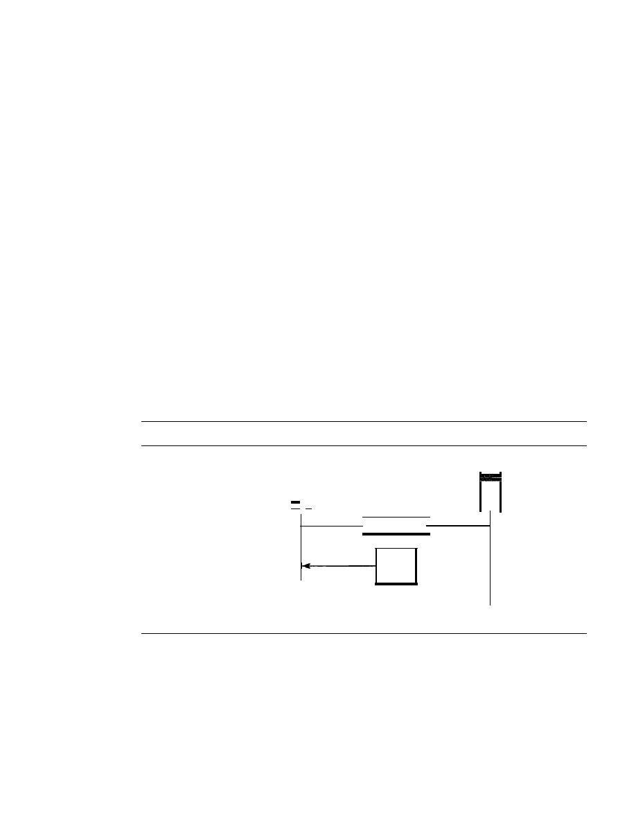
860
CHAPTER
27
WWW AND HTTP
Active Documents
For many applications, we need a program or a script to be run at the client site. These
are called
active documents.
For example, suppose we want to run a program that
creates animated graphics on the screen or a program that interacts with the user. The
program definitely needs to be run at the client site where the animation or interaction
takes place. When a browser requests an active document, the server sends a copy of the
document or a script. The document is then run at the client (browser) site.
Java Applets
One way to create an active document is to use Java
applets. Java
is a combination of a
high-level programming language, a run-time environment, and a class library that
allows a programmer to write an active document (an applet) and a browser to run it.
It
can also be a stand-alone program that doesn't use a browser.
An applet is a program written in Java on the server.
It
is compiled and ready to be
run. The document is in byte-code (binary) format. The client process (browser) creates
an instance of this applet and runs it. A Java applet can be run by the browser in two
ways. In the first method, the browser can directly request the Java applet program in
the URL and receive the applet in binary form. In the second method, the browser can
retrieve and run an HTML file that has embedded the address of the applet as a tag. Fig-
ure 27.10 shows how Java applets are used in the first method; the second is similar but
needs two transactions.
Figure 27.10
Active document using Java applet
Client
-
Request
Server
Applet
t - - - - - - I
Run the applet
to get the result
Result
JavaScript
The idea of scripts in dynamic documents can also be used for active documents.
If
the
active part of the document is small, it can be written in a scripting language; then it can
be interpreted and run by the client at the same time. The script is in source code (text)
and not in binary form. The scripting technology used in this case is usually JavaScript.
JavaScript,
which bears a small resemblance to Java, is a very high level scripting
language developed for this purpose. Figure 27.11 shows how JavaScript is used to create
an active document.
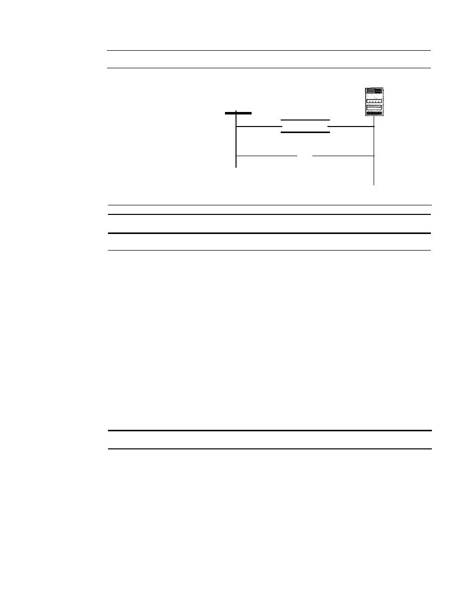
SECTION
27.3
HTTP
861
Figure 27.11
Active document using client-site script
Server
Client
Request
Run the JavaScript (JS)
to get the result
Result
Active documents are sometimes referred to as client-site dynamic documents.
27.3
HTTP
The Hypertext Transfer Protocol (HTTP) is a protocol used mainly to access data on
the World Wide Web. HTTP functions as a combination of FTP and SMTP.
It
is similar to
FfP
because it transfers files and uses the services of TCP. However, it is much simpler
than
FfP
because it uses only one TCP connection. There is no separate control connec-
tion; only data are transferred between the client and the server.
HTTP is like SMTP because the data transferred between the client and the server
look like SMTP messages. In addition, the format of the messages is controlled by
MIME-like headers. Unlike SMTP, the HTTP messages are not destined to be read by
humans; they are read and interpreted by the HTTP server and HTTP client (browser).
SMTP messages are stored and forwarded, but HTTP messages are delivered immedi-
ately. The commands from the client to the server are embedded in a request message.
The contents of the requested file or other information are embedded in a response
message. HTTP uses the services of TCP on well-known port 80.
HTTP uses the services of TCP on well-known port 80.
HTTP Transaction
Figure 27.12 illustrates the HTTP transaction between the client and server. Although
HTTP uses the services of TCP, HTTP itself is a stateless protocol. The client initializes
the transaction by sending a request message. The server replies by sending a response.
Messages
The formats of the request and response messages are similar; both are shown in Fig-
ure 27.13. A request message consists of a request line, a header, and sometimes a body.
A response message consists of a status line, a header, and sometimes a body.
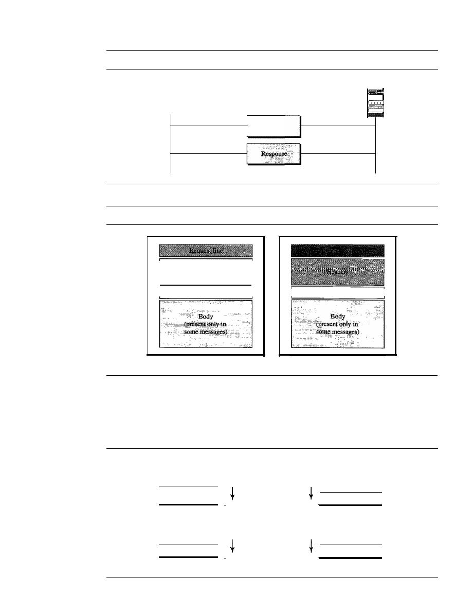
862
CHAPTER
27
WWW AND HTTP
Figure 27.12
HTTP transaction
Client
Request
Figure 27.13
Request and response messages
Headers
A blank line
Request message
Server
A blank line
Response message
Request and Status Lines
The first line in a request message is called a request line;
the first line in the response message is called the status line. There is one common
field, as shown in Figure 27.14.
Figure 27.14
Request and status lines
Space
Space
Request type
I
I
HTTP version
a. Request line
Space
Space
I
I
HTTP version
Status phrase
b. Status line

SECTION
27.3
HTTP
863
o
Request type. This field is used in the request message. In version
1.1 of HTTP,
several request types are defined. The request type is categorized into
methods
as
defined in Table
27.1.
Table 27.1
Methods
Method
Action
GET
Requests a document from the server
HEAD
Requests information about a document but not the document itself
POST
Sends some information from the client to the server
PUT
Sends a document from the server to the client
TRACE
Echoes the incoming request
CONNECT
Reserved
OPTION
Inquires about available options
o
URL. We discussed the URL earlier in the chapter.
o
Version. The most current version of HTTP is 1.1.
o
Status code. This field is used in the response message. The status code field is
similar to those in the FTP and the SMTP protocols.
It
consists of three digits.
Whereas the codes in the 100 range are only informational, the codes in the 200
range indicate a successful request. The codes in the 300 range redirect the client
to another URL, and the codes in the 400 range indicate an error at the client site.
Finally, the codes in the 500 range indicate an error at the server site. We list the
most common codes in Table
27.2.
o
Status phrase. This field is used in the response message.
It
explains the status
code in text form. Table
27.2 also gives the status phrase.
Table 27.2
Status codes
Code
Phrase
Description
Informational
100
Continue
The initial part of the request has been received, and the
client may continue with its request.
101
Switching
The server is complying with a client request to switch
protocols defined in the upgrade header.
Success
200
OK
The request is successful.
201
Created
A new URL is created.
202
Accepted
The request is accepted, but it is not immediately acted upon.
204
No content
There is no content in the body.

864
CHAPTER
27
WWW AND HITP
Table 27.2
Status codes (continued)
Code
Phrase
Description
Redirection
301
Moved permanently
The requested URL is no longer used by the server.
302
Moved temporarily
The requested URL has moved temporarily.
304
Not modified
The document has not been modified.
Client Error
400
Bad request
There is a syntax error in the request.
401
Unauthorized
The request lacks proper authorization.
403
Forbidden
Service is denied.
404
Not found
The document is not found.
405
Method not allowed
The method is not supported in this URL.
406
Not acceptable
The format requested is not acceptable.
Server Error
500
Internal server error
There is an error, such as a crash, at the server site.
501
Not implemented
The action requested cannot be performed.
503
Service unavailable
The service is temporarily unavailable, but may be requested
in the future.
Header
The header exchanges additional information between the client and the server.
For example, the client can request that the document be sent in a special format, or the
server can send extra information about the document. The header can consist of one or
more header lines. Each header line has a header name, a colon, a space, and a header
value (see Figure 27.15). We will show some header lines in the examples at the end of
this chapter.
A
header line belongs to one of four categories:
general header, request
header, response header,
and
entity header. A
request message can contain only gen-
eral, request, and entity headers. A response message, on the other hand, can contain only
general, response, and entity headers.
Figure 27.15
Header format
Space
I
Header name
I
Header value
o
General header
The general header gives general information about the message
and can be present in both a request and a response. Table 27.3 lists some general
headers with their descriptions.

SECTION
27.3
HTTP
865
Table 27.3
General headers
Header
Description
Cache-control
Specifies infonnation about caching
Connection
Shows whether the connection should be closed or not
Date
Shows the current date
MIME-version
Shows the MIME version used
Upgrade
Specifies the preferred communication protocol
o
Request header The request header can be present only in a request message.
It
specifies the client's configuration and the client's preferred document format. See
Table 27.4 for a list of some request headers and their descriptions.
Table 27.4
Request headers
Header
Description
Accept
Shows the medium fonnat the client can accept
Accept-charset
Shows the character set the client can handle
Accept-encoding
Shows the encoding scheme the client can handle
Accept-language
Shows the language the client can accept
Authorization
Shows what pennissions the client has
From
Shows the e-mail address of the user
Host
Shows the host and port number of the server
If-modified-since
Sends the document if newer than specified date
If-match
Sends the document only if it matches given tag
If-non-match
Sends the document only if it does not match given tag
--
_._---.
. .
_-
If-range
Sends only the portion of the document that is missing
If-unmodified-since
Sends the document if not changed since specified date
Referrer
Specifies the URL of the linked document
User-agent
Identifies the client program
o
Response header The response header can be present only in a response message.
It
specifies the server's configuration and special information about the request.
See Table 27.5 for a list of some response headers with their descriptions.
Table 27.5
Response headers
Header
Description
Accept-range
Shows if server accepts the range requested by client
Age
Shows the age of the document
Public
Shows the supported list of methods
Retry-after
Specifies the date after which the server is available
Server
Shows the server name and version number
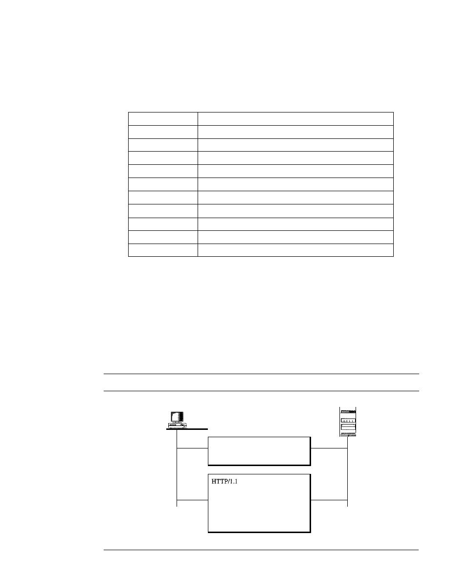
866
CHAPTER
27
WWW AND HTTP
o
Entity header The entity header gives infonnation about the body of the docu-
ment. Although it is mostly present in response messages, some request messages,
such as POST or PUT methods, that contain a body also use this type of header.
See Table 27.6 for a list of some entity headers and their descriptions.
Table 27.6
Entity headers
Header
Description
Allow
Lists valid methods that can be used with a URL
Content-encoding
Specifies the encoding scheme
Content-language
Specifies the language
Content-length
Shows the length of the document
Content-range
Specifies the range of the document
Content-type
Specifies the medium type
Etag
Gives an entity tag
Expires
Gives the date and time when contents may change
Last-modified
Gives the date and time of the last change
Location
Specifies the location of the created or moved document
Body
The body can be present in a request or response message. Usually, it contains
the document to be sent or received.
Example 27.1
This example retrieves a document. We use the GET method to retrieve an image with the
path /usr/bin/imagel. The request line shows the method (GET), the URL, and the HTTP ver-
sion
(1.1).
The header has two lines that show that the client can accept images in the GIF or
JPEG format. The request does not have a body. The response message contains the status line
and four lines of header. The header lines define the date, server, MIME version, and length of the
document. The body of the document follows the header (see Figure 27.16).
Figure 27.16
Example 27.1
Server
cr
t
len
=
Request (GET method)
GET lusrlbinlimage1
HTTP/l.l
Accept: image/gif
Accept: image/jpeg
200 OK
Date: Mon, 07-Jan-05 13:15:14 GMT
Server: Challenger
MIME-version: l.0
Content-length: 2048
(Body
of the document)
Response
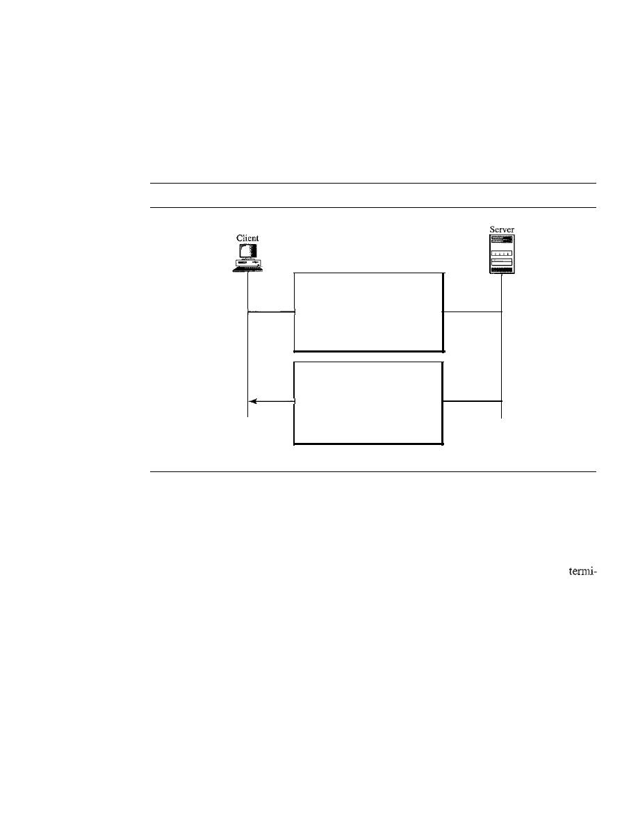
SECTION
27.3
HTTP
867
Example 27.2
In
this example, the client wants to send data to the server. We use the POST method. The request
line shows the method (POST), URL, and HTTP version (1.1). There are four lines of headers.
The request body contains the input information. The response message contains the status line
and four lines of headers. The created document, which is a CGI document, is included as the body
(see Figure 27.17).
Figure 27.17
Example 27.2
Request (POST method)
POST /cgi-binldoc.pl HTIP/1.l
Accept: */*
Accept: image/gif
Accept: image/jpeg
Content-length:
50
(Input information)
HTTP/l.1 200 OK
Date: Mon, 07-Jan-02 13:15:14 GMT
Server: Challenger
MIME-version: 1.0
Content-length: 2000
(Body of the document)
Response
Example 27.3
HTTP uses ASCII characters. A client can directly connect to a server using TELNET, which
logs into port 80. The next three lines show that the connection is successful.
We then type three lines. The first shows the request line (GET method), the second is the
header (defining the host), the third is a blank, terminating the request.
The server response is seven lines starting with the status line. The blank line at the end
nates the server response. The file of 14,230 lines is received after the blank line (not shown here).
The last line is the output by the client.
$
teinet www.mhhe.com 80
Trying 198.45.24.104 ...
Connected to www.mhhe.com (198.45.24.104).
Escape character is 11\]'.
GET
/engcslcompscilforouzan HTTP/I.t
From: forouzanbehrouz@fbda.edu
HTTP/t.l 200 OK
Date: Thu, 28 Oct 2004 16:27:46 GMT
Server: Apache/l.3.9 (Unix) ApacheJServ/1.1.2 PHP/4.1.2 PHP/3.0.18
MIME-version:1.0
Content-Type: text/html

868
CHAPTER
27
WWW AND HTTP
Last-modified: Friday, 15-0ct-04 02:11:31 GMT
Content-length: 14230
Connection closed by foreign host.
Persistent Versus Nonpersistent Connection
HTTP prior to version 1.1 specified a nonpersistent connection, while a persistent con-
nection is the default in version 1.1.
Nonpersistent Connection
In a
nonpersistent connection,
one TCP connection is made for each request/response.
The following lists the steps in this strategy:
1.
The client opens a TCP connection and sends a request.
2. The server sends the response and closes the connection.
3. The client reads the data until it encounters an end-of-file marker; it then closes the
connection.
In this strategy, for
N
different pictures in different files, the connection must be opened
and closed N times. The nonpersistent strategy imposes high overhead on the server
because the server needs
N
different buffers and requires a slow start procedure each
time a connection is opened.
Persistent Connection
HTTP version 1.1 specifies a
persistent connection
by default.
In
a persistent connection,
the server leaves the connection open for more requests after sending a response. The
server can close the connection at the request of a client or if a time-out has been reached.
The sender usually sends the length of the data with each response. However, there are
some occasions when the sender does not know the length of the data. This is the case
when a document is created dynamically or actively. In these cases, the server informs
the client that the length is not known and closes the connection after sending the data so
the client knows that the end of the data has been reached.
HTTP version 1.1 specifies a persistent connection by default.
Proxy Server
HTTP supports
proxy servers.
A proxy server is a computer that keeps copies of
responses to recent requests. The HTTP client sends a request to the proxy server. The
proxy server checks its cache.
If
the response is not stored in the cache, the proxy
server sends the request to the corresponding server. Incoming responses are sent
to
the
proxy server and stored for future requests from other clients.
The proxy server reduces the load on the original server, decreases traffic, and
improves latency. However, to use the proxy server, the client must be configured to
access the proxy instead of the target server.

SECTION
27.5
KEY TERMS
869
27.4
RECOMMENDED READING
For more details about subjects discussed in this chapter, we recommend the following
books and sites. The items in brackets [...] refer to the reference list at the end of the text.
Books
HTTP is discussed in Chapters 13 and 14 of [Ste96], Section 9.3 of [PD03], Chapter 35
of [Com04], and Section 7.3 of [Tan03].
Sites
The following sites are related to topics discussed in this chapter.
o
www.ietf.org/rfc.html
Information about RFCs
RFCs
The following RFCs are related to WWW:
1614,1630,1737,1738
The following RFCs are related to HTTP:
2068,2109
27.5
KEY TERMS
active document
Active Server Pages (ASP)
applet
browser
ColdFusion
Common Gateway Interface (CGI)
dynamic document
entity header
general header
host
Hypertext Markup Language
(HTML)
Hypertext Preprocessor (PHP)
Hypertext Transfer Protocol (HTTP)
Java
JavaScript
Java Server Pages (JSP)
nonpersistent connection
path
persistent connection
proxy server
request header
request line
request type
response header
static document
status code
status line
tag
uniform resource locator (URL)
Web
World Wide Web (WWW)

870
CHAPTER
27
WWW AND HITP
27.6
SUMMARY
o
The World Wide Web (WWW) is a repository of information linked together from
points all over the world.
o
Hypertexts are documents linked to one another through the concept of pointers.
o
Browsers interpret and display a Web document.
o
A browser consists of a controller, client programs, and interpreters.
o
A Web document can be classified as static, dynamic, or active.
o
A static document is one in which the contents are fixed and stored in a server. The
client can make no changes in the server document.
o
Hypertext Markup Language (HTML) is a language used to create static Web pages.
o
Any browser can read formatting instructions (tags) embedded in an HTML
document.
o
Tags provide structure to a document, define titles and headers, format text, control
the data flow, insert figures, link different documents together, and define execut-
able code.
o
A dynamic Web document is created by a server only at a browser request.
o
The Common Gateway Interface (CGI) is a standard for creating and handling
dynamic Web documents.
o
A CGI program with its embedded CGI interface tags can be written in a language
such as C, C++, Shell Script, or Perl.
o
An active document is a copy of a program retrieved by the client and run at the
client site.
o
Java is a combination of a high-level programming language, a run-time environ-
ment, and a class library that allows a programmer to write an active document and
a browser to run it.
o
Java is used to create applets (small application programs).
o
The Hypertext Transfer Protocol (HTTP) is the main protocol used to access data
on the World Wide Web (WWW).
o
HTTP uses a TCP connection to transfer files.
o
An HTTP message is similar in form to an SMTP message.
o
The HTTP request line consists of a request type, a URL, and the HTTP version
number.
o
The uniform resource locator (URL) consists of a method, host computer, optional
port number, and path name to locate information on the WWW.
o
The HTTP request type or method is the actual command or request issued by the
client to the server.
o
The status line consists of the HTTP version number, a status code, and a status
phrase.
o
The HTTP status code relays general information, information related to a successful
request, redirection information, or error information.
o
The HTTP header relays additional information between the client and server.

SECTION 27. 7
PRACTICE SET
871
D
An HTTP header consists of a header name and a header value.
D
An HTTP general header gives general information about the request or response
message.
D
An HTTP request header specifies a client's configuration and preferred document
format.
D
An HTTP response header specifies a server's configuration and special information
about the request.
D
An HTTP entity header provides information about the body of a document.
D
HTTP, version 1.1, specifies a persistent connection.
D
A proxy server keeps copies of responses to recent requests.
27.7
PRACTICE SET
Review Questions
1. How is HTTP related to WWW?
2. How is HTTP similar to SMTP?
3. How is HTTP similar to
FTP?
4. What is a URL and what are its components?
5. What is a proxy server and how is it related to HTTP?
6. Name the common three components of a browser.
7. What are the three types of Web documents?
8. What does HTML stand for and what is its function?
9. What is the difference between an active document and a dynamic document?
10. What does CGI stand for and what is its function?
11. Describe the relationship between Java and an active document.
Exercises
12. Where will each figure be shown on the screen?
Look at the following picture:
then tell me what you feel:
<IMG SRC="PictureslFunnyl.gif" ALIGN=middle>
<lMG SRC="Pictures/Funny2.gif" ALIGN=bottom>
<B>What is your feeling? <IE>
13. Show the effect of the following HTML segment.
The publisher of this book is <A HREF="www.mhhe">
McGraw-Hill Publisher
<fA>
14. Show a request that retrieves the document /usr/users/doc/docl. Use at least two
general headers, two request headers, and one entity header.
15. Show the response to Exercise 14 for a successful request.
16. Show the response to Exercise 14 for a document that has permanently moved to
/usr/deads/doc1.

872
CHAPTER
27
WWW AND HTTP
17. Show the response to Exercise 14 if there is a syntax error in the request.
18. Show the response to Exercise 14 if the client is unauthorized to access the document.
19. Show a request that asks for information about a document at /bin/users/file. Use at
least two general headers and one request header.
20. Show the response to Exercise 19 for a successful request.
21. Show the request to copy the file at location /bin/usr/bin/file 1 to /bin/file1.
22. Show the response to Exercise 21.
23. Show the request to delete the file at location /bin/file!.
24. Show the response to Exercise 23.
25. Show a request to retrieve the file at location /bin/etc/file!. The client needs the
document only if it was modified after January 23, 1999.
26. Show the response to Exercise 25.
27. Show a request to retrieve the file at location /bin/etc/filel. The client should iden-
tify itself.
28. Show the response to Exercise 27.
29. Show a request to store a file at location /bin/letter. The client identifies the types
of documents it can accept.
30. Show the response to Exercise 29. The response shows the age of the document as
well as the date and time when the contents may change.
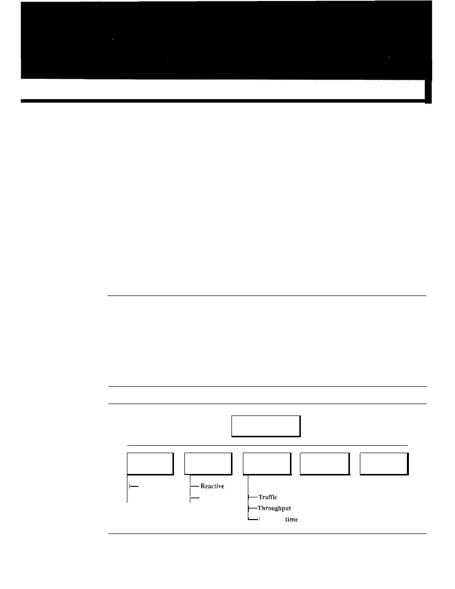
CHAPTER 28
Network Management: SNMP
We can define network management as monitoring, testing, configuring, and trouble-
shooting network components to meet a set of requirements defined by an organiza-
tion. These requirements include the smooth, efficient operation of the network that
provides the predefined quality of service for users. To accomplish this task, a network
management system uses hardware, software, and humans. In this chapter, first we
briefly discuss the functions of a network management system. Then we concentrate
on the most common management system, the Simple Network Management Protocol
(SNMP).
28.1
NETWORK MANAGEMENT SYSTEM
We can say that the functions performed by a network management system can be
divided into five broad categories: configuration management, fault management, per-
formance management, security management, and accounting management, as shown
in Figure 28.1.
Figure 28.1
Functions of a network management system
Response
Functions of a network
management system
I
I
I
I
I
I
Configuration
Fault
Performance
Security
Accounting
management
management
management
management
management
Reconfiguration
-Capacity
'--Documentation
Proactive
873

874
CHAPTER
28
NETWORK MANAGEMENT: SNMP
Configuration Management
A large network is usually made up of hundreds of entities that are physically or logically
connected to one another. These entities have an initial configuration when the network
is set up, but can change with time. Desktop computers may be replaced by others;
application software may be updated to a newer version; and users may move from one
group to another. The configuration management system must know, at any time, the
status of each entity and its relation to other entities. Configuration management can
be divided into two subsystems: reconfiguration and documentation.
Reconfiguration
Reconfiguration, which means adjusting the network components and features, can be a
daily occurrence in a large network. There are three types of reconfiguration: hardware
reconfiguration, software reconfiguration, and user-account reconfiguration.
Hardware reconfiguration covers all changes to the hardware. For example, a desk-
top computer may need to be replaced. A router may need to be moved to another part
of the network. A subnetwork may be added or removed from the network. All these
need the time and attention of network management. In a large network, there must be
specialized personnel trained for quick and efficient hardware reconfiguration. Unfortu-
nately, this type of reconfiguration cannot be automated and must be manually handled
case by case.
Software reconfiguration covers all changes to the software. For example, new
software may need to be installed on servers or clients. An operating system may need
updating. Fortunately, most software reconfiguration can be automated. For example,
updating an application on some or all clients can be electronically downloaded from
the server.
User-account reconfiguration is not simply adding or deleting users on a system.
You must also consider the user privileges, both as an individual and as a member of a
group. For example, a user may have read and write permission with regard to some
files, but only read permission with regard to other files. User-account reconfiguration
can be, to some extent, automated. For example, in a college or university, at the begin-
ning of each quarter or semester, new students are added to the system. The students are
normally grouped according to the courses they take or the majors they pursue.
Documentation
The original network configuration and each subsequent change must be recorded
meticulously. This means that there must be documentation for hardware, software, and
user accounts.
Hardware documentation normally involves two sets of documents: maps and
specifications. Maps track each piece of hardware and its connection to the network.
There can be one general map that shows the logical relationship between each subnet-
work. There can also be a second general map that shows the physical location of each
subnetwork. For each subnetwork, then, there is one or more maps that show all pieces
of equipment. The maps use some kind of standardization to be easily read and under-
stood by current and future personnel. Maps are not enough per se. Each piece of hard-
ware also needs to be documented. There must be a set of specifications for each piece

SECTION
28.1
NETWORK MANAGEMENT SYSTEM
875
of hardware connected to the network. These specifications must include information
such as hardware type, serial number, vendor (address and phone number), time of
purchase, and warranty information.
All software must also be documented. Software documentation includes informa-
tion such as the software type, the version, the time installed, and the license agreement.
Most operating systems have a utility that allows the documentation of user accounts
and their privileges. The management must make sure that the files with this information
are updated and secured. Some operating systems record access privileges in two docu-
ments; one shows all files and access types for each user; the other shows the list of users
that have a particular access to a file.
Fault Management
Complex networks today are made up of hundreds and sometimes thousands of compo-
nents. Proper operation of the network depends on the proper operation of each component
individually and in relation to each other.
Fault management
is the area of network
management that handles this issue.
An effective fault management system has two subsystems: reactive fault manage-
ment and proactive fault management.
Reactive Fault Management
A reactive fault management system is responsible for detecting, isolating, correcting,
and recording faults.
It
handles short-term solutions to faults.
The first step taken by a reactive fault management system is to detect the exact
location of the fault. A fault is defined as an abnormal condition in the system. When a
fault occurs, either the system stops working properly or the system creates excessive
errors. A good example of a fault is a damaged communication medium. This fault may
interrupt communication or produce excessive errors.
The next step taken by a reactive fault management system is to isolate the fault. A
fault, if isolated, usually affects only a few users. After isolation, the affected users are
immediately notified and given an estimated time of correction.
The third step is to correct the fault. This may involve replacing or repairing the
faulty component(s).
After the fault is corrected, it must be documented. The record should show the
exact location of the fault, the possible cause, the action or actions taken to correct the
fault, the cost, and time it took for each step. Documentation is extremely important for
several reasons:
o
The problem may recur. Documentation can help the present or future administrator
or technician solve a similar problem.
o
The frequency of the same kind of failure is an indication of a major problem in
the system. If a fault happens frequently in one component, it should be replaced
with a similar one, or the whole system should be changed to avoid the use of that
type of component.
o
The statistic is helpful to another part of network management, performance
management.

876
CHAPTER
28
NETWORK MANAGEMENT: SNMP
Proactive Fault Management
Proactive fault management tries to prevent faults from occurring. Although this is not
always possible, some types of failures can be predicted and prevented. For example, if
a manufacturer specifies a lifetime for a component or a part of a component,
it
is a
good strategy to replace it before that time. As another example, if a fault happens
frequently at one particular point of a network, it is wise to carefully reconfigure the
network to prevent the fault from happening again.
Performance Management
Performance management,
which is closely related to fault management, tries to
monitor and control the network to ensure that it is running as efficiently as possible.
Performance management tries to quantify performance by using some measurable
quantity such as capacity, traffic, throughput, or response time.
Capacity
One factor that must be monitored by a performance management system is the capacity
of the network. Every network has a limited capacity, and the performance management
system must ensure that it is not used above this capacity. For example, if a LAN is
designed for 100 stations at an average data rate of2 Mbps, it will not operate properly if
200 stations are connected to the network. The data rate will decrease and blocking
may occur.
Traffic
Traffic can be measured in two ways: internally and externally. Internal traffic is
sured by the number of packets (or bytes) traveling inside the network. External traffic
is measured by the exchange of packets (or bytes) outside the network. During peak
hours, when the system is heavily used, blocking may occur if there is excessive traffic.
Throughput
We can measure the throughput of an individual device (such as a router) or a part of
the network. Performance management monitors the throughput to make sure that it is
not reduced to unacceptable levels.
Response Time
Response time is normally measured from the time a user requests a service to the time
the service is granted. Other factors such as capacity and traffic can affect the response
time. Performance management monitors the average response time and the peak-hour
response time. Any increase in response time is a very serious condition as it is an indi-
cation that the network is working above its capacity.
Security Management
Security management
is responsible for controlling access to the network based on
the predefined policy. We discuss security and in particular network security in Chap-
ters 31 and 32.
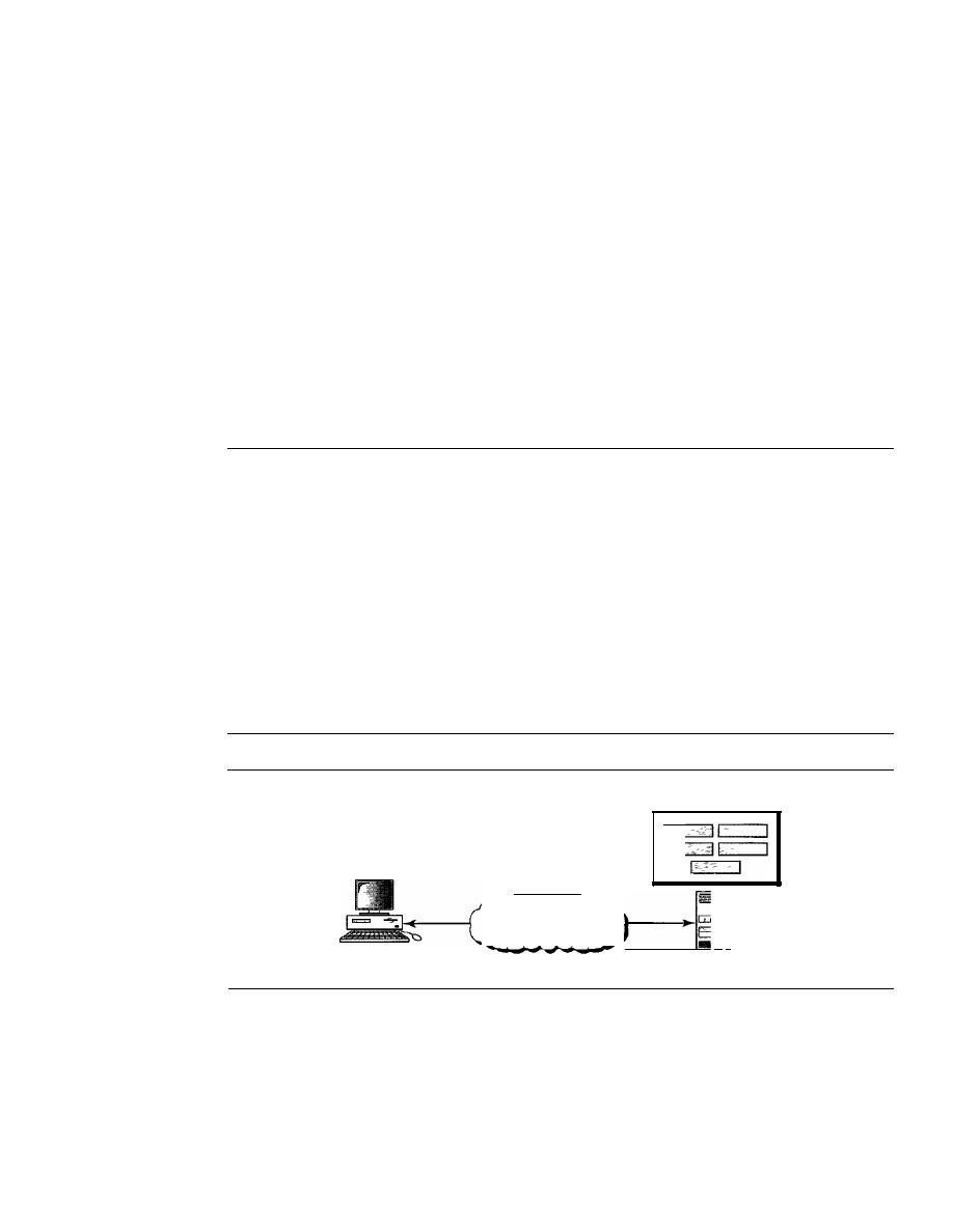
SECTION
28.2
SIMPLE NETWORK MANAGEMENT PROTOCOL (SNMP)
877
Accounting Management
Accounting management is the control of users' access to network resources through
charges. Under accounting management, individual users, departments, divisions, or
even projects are charged for the services they receive from the network. Charging does
not necessarily mean cash transfer; it may mean debiting the departments or divisions
for budgeting purposes. Today, organizations use an accounting management system
for the following reasons:
o
It prevents users from monopolizing limited network resources.
o
It prevents users from using the system inefficiently.
o
Network managers can do short- and long-term planning based on the demand for
network use.
28.2
SIMPLE NETWORK MANAGEMENT
PROTOCOL (SNMP)
The Simple Network Management Protocol (SNMP) is a framework for managing
devices in an internet using the TCPIIP protocol suite. It provides a set of fundamental
operations for monitoring and maintaining an internet.
Concept
SNMP uses the concept of manager and agent. That is, a manager, usually a host,
controls and monitors a set of agents, usually routers (see Figure 28.2).
Figure 28.2
SNMP concept
Agent variables
Agent
Internet
:'
:1
Manager
SNMP is an application-level protocol in which a few manager stations control a
set of agents. The protocol is designed at the application level so that it can monitor
devices made by different manufacturers and installed on different physical networks.
In other words, SNMP frees management tasks from both the physical characteristics
of the managed devices and the underlying networking technology. It can be used in a
heterogeneous internet made of different LANs and WANs connected by routers made
by different manufacturers.

878
CHAPTER
28
NETWORK MANAGEMENT: SNMP
Managers and Agents
A management station, called a
manager,
is a host that runs the SNMP client program. A
managed station, called an
agent,
is a router (or a host) that runs the SNMP server program.
Management is achieved through simple interaction between a manager and an agent.
The agent keeps performance information in a database. The manager has access
to the values in the database. For example, a router can store in appropriate variables
the number of packets received and forwarded. The manager can fetch and compare the
values of these two variables to see if the router is congested or not.
The manager can also make the router perform certain actions. For example, a
router periodically checks the value of a reboot counter to see when it should reboot
itself. It reboots itself, for example, if the value of the counter is O. The manager can
use this feature to reboot the agent remotely at any time.
It
simply sends a packet to
force a 0 value in the counter.
Agents can also contribute to the management process. The server program running
on the agent can check the environment, and if it notices something unusual, it can send
a warning message, called a
trap,
to the manager.
In other words, management with SNMP is based on three basic ideas:
1. A manager checks an agent by requesting information that reflects the behavior of
the agent.
2. A manager forces an agent to perform a task by resetting values
in
the agent database.
3. An agent contributes to the management process by warning the manager of an
unusual situation.
Management Components
To do management tasks, SNMP uses two other protocols:
Structure of Management
Information (SMI)
and
Management Information Base (MIB).
In other words, man-
agement on the Internet is done through the cooperation of the three protocols SNMP,
SMI, and MIB, as shown in Figure 28.3.
Figure 28.3
Components of network management on the Internet
Management
I
SNMP
8MI
MIB
I
Let us elaborate on the interactions between these protocols.
RoleofSNMP
SNMP has some very specific roles in network management.
It
defines the format of
the packet to be sent from a manager to an agent and vice versa.
It
also interprets the

SECTION
28.2
SIMPLE NETWORK MANAGEMENT PROTOCOL (SNMP)
879
result and creates statistics (often with the help of other management software). The
packets exchanged contain the object (variable) names and their status (values). SNMP
is responsible for reading and changing these values.
SNMP defines the format of packets exchanged between a manager and an agent.
It reads and changes the status (values) of objects (variables) in 8NMP packets.
Role ofSMI
To use SNMP, we need rules. We need rules for naming objects. This is particularly
important because the objects in SNMP form a hierarchical structure (an object may
have a parent object and some children objects). Part of a name can be inherited from
the parent. We also need rules to define the type of the objects. What types of objects
are handled by SNMP? Can SNMP handle simple types or structured types? How many
simple types are available? What are the sizes of these types? What is the range of these
types? In addition, how are each of these types encoded?
We need these universal rules because we do not know the architecture of the com-
puters that send, receive, or store these values. The sender may be a powerful computer
in which an integer is stored as 8-byte data; the receiver may be a small computer that
stores an integer as 4-byte data.
SMI is a protocol that defines these rules. However, we must understand that SMI
only defines the rules; it does not define how many objects are managed in an entity or
which object uses which type. SMI is a collection of general rules to name objects and
to list their types. The association of an object with the type is not done by SMI.
8MI defines the general rules for naming objects, defining object types (including
range and length), and showing how to encode objects and values.
8M1 does not define the number of objects an entity should manage or name the objects
to be managed or define the association between the objects and their values.
Role ofMIB
We hope it is clear that we need another protocol. For each entity to be managed, this
protocol must define the number of objects, name them according to the rules defined
by SMI, and associate a type to each named object. This protocol is MIB. MIB creates
a set of objects defined for each entity similar to a database (mostly metadata in a data-
base, names and types without values).
creates a collection of named objects, their types, and their relationships to
each other in an entity to be managed.
An Analogy
Before discussing each of these protocols in greater detail, we give an analogy. The
three network management components are similar to what we need when we write a
program in a computer language to solve a problem.

880
CHAPTER
28
NETWORK MANAGEMENT: SNMP
Before we write a program, the syntax of the language (such as C or Java) must be
predefined. The language also defines the structure of variables (simple, structured,
pointer, and so on) and how the variables must be named. For example, a variable name
must be
1
to
N
characters in length and start with a letter followed by alphanumeric
characters. The language also defines the type of data to be used (integer, float, char,
etc.). In programming the rules are defined by the language. In network management
the rules are defined by SMI.
Most computer languages require that variables be declared in each specific pro-
gram. The declaration names each variable and defines the predefined type. For example,
if a program has two variables (an integer named
counter
and an array named
grades
of
type char), they must be declared at the beginning of the program:
int
counter;
char
grades
[40];
Note that the declarations name the variables (counter and grades) and define the
type of each variable. Because the types are predefined in the language, the program
knows the range and size of each variable.
MIB does this task in network management.
MIB
names each object and defines
type of the objects. Because the type is defined by SMI, SNMP knows the range and size.
After declaration in programming, the program needs to write statements to store
values in the variables and change them if needed. SNMP does this task in network
management. SNMP stores, changes, and interprets the values of objects already
declared by MIB according to the rules defined by SMI.
We can compare the task of network management to
the
task of writing
a
program.
o
Both tasks need rules.
In
network management this is handled by SMI.
o
Both tasks need variable declarations.
In
network management this is handled by MIB.
o
Both tasks have actions performed by statements. In network management this is
handled by SNMP.
An Overview
Before discussing each component in detail, we show how each is involved in a simple
scenario. This is an overview that will be developed later at the end of the chapter. A
manager station (SNMP client) wants to send a message to an agent station (SNMP
server) to find the number of UDP user datagrams received by the agent. Figure 28.4
shows an overview of steps involved.
MIB is responsible for finding the object that holds the number of the UDP user
datagrams received. SMI, with the help of another embedded protocol, is responsible for
encoding the name of the object. SNMP is responsible for creating a message, called a
GetRequest message, and encapsulating the encoded message. Of course, things are
more complicated than this simple overview, but we first need more details of each
protocol.
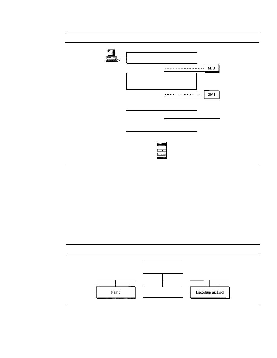
SECTION
28.2
SIMPLE NETWORK MANAGEMENT PROTOCOL (SNMP)
881
Figure 28.4
Management overview
Number of UDP user datagrams?
The object has an integer value and
is called udpInDatagram with id
1.3.6.1.2.1.7.1.0
Retrieve the value of an object
with code 06 09
.
--------------jSNMPI
Encapsulate the request in a
GetRequest message
Structure
of Management Information
The Structure of Management Information, version 2 (SMIv2) is a component for net-
work management. Its functions are
1. To name objects
2. To define the type of data that can be stored in an object
3. To show how to encode data for transmission over the network
SMI is a guideline for SNMP.
It
emphasizes three attributes to handle an object: name,
data type, and encoding method (see Figure 28.5).
Figure 28.5
Object attributes
Object attributes
Type
Name
SMI requires that each managed object (such as a router, a variable in a router, a value)
have a unique name. To name objects globally, SMI uses an
object identifier,
which is
a hierarchical identifier based on a tree structure (see Figure 28.6).
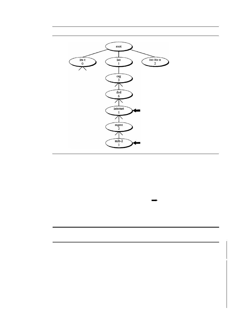
882
CHAPTER
28
NETWORK MANAGEMENT: SNMP
Figure 28.6
Object identifier
1.3.6.1 (iso.org.dop.intemet)
1.3.6.1.2.1 (iso.org.dod.internet.mgmt.mib-2)
The tree structure starts with an unnamed root. Each object can be defined by using
a sequence of integers separated by dots. The tree structure can also define an object by
using a sequence of textual names separated by dots. The integer-dot representation is
used in SNMP. The name-dot notation is used by people. For example, the following
shows the same object in two different notations:
iso.org.dod.internet.mgmt.mib-2
1.3.6.1.2.1
The objects that are used in SNMP are located under the
mib-2
object, so their
identifiers always start with 1.3.6.1.2.1.
AU objects managed by SNMP are given an object identifier.
The object identifier always starts with 1.3.6.1.2.1.
Type
The second attribute of an object is the type of data stored in it. To define the data type,
SMI uses fundamental
Abstract Syntax Notation 1 (ASN.l) definitions and adds
some new definitions. In other words, SMI is both a subset and a superset of ASN.1.
SMI has two broad categories of data type:
simple
and
structured.
We first define
the simple types and then show how the structured types can be constructed from the
simple ones (see Figure 28.7).
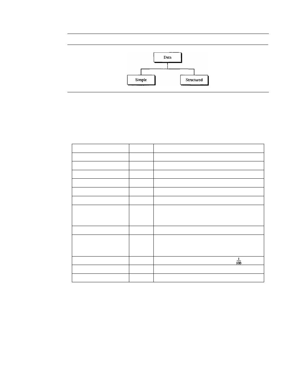
SECTION
28.2
SIMPLE NEIWORK MANAGEMENT PROTOCOL (SNMP)
883
Figure 28.7
Data type
Simple Type
The simple data types are atomic data types. Some of them are taken
directly from ASN.l; others are added by SMI. The most important ones are given in
Table 28.1. The first five are from ASN.l; the next seven are defined by SMI.
Table 28.1
Data types
Type
Size
Description
INTEGER
4 bytes
An integer with a value between _2
31
and 2
31
-
1
Integer32
4 bytes
Same as INTEGER
Unsigned32
4 bytes
Unsigned with a value between 0 and 2
32
-
1
OCTET STRING
Variable
Byte string up to 65,535 bytes long
OBJECT IDENTIFIER
Variable
An object identifier
IPAddress
4 bytes
An IP address made of four integers
Counter32
4 bytes
An integer whose value can be incremented
from 0 to 2
32
;
when
it
reaches its maximum
value, it wraps back to
O.
Counter64
8 bytes
64-bit counter
Gauge32
4 bytes
Same as Counter32, but when it reaches its
maximum value, it does not wrap; it remains
there until it is reset
TimeTicks
4 bytes
A counting value that records time in
s
BITS
A string of bits
Opaque
Variable
Uninterpreted string
Structured Type
By combining simple and structured data types, we can make new
structured data types. SMI defines two structured
data types:
sequence
and
sequence of
o
Sequence. A
sequence
data type is a combination of simple data types, not neces-
sarily of the same type.
It
is analogous to the concept of a
struct
or a
record
used in
programming languages such as C.
o
Sequence of. A
sequence of
data type is a combination of simple data types all of
the same type or a combination of sequence data types all of the same type. It is
analogous to the concept of an
array
used in programming languages such as C.
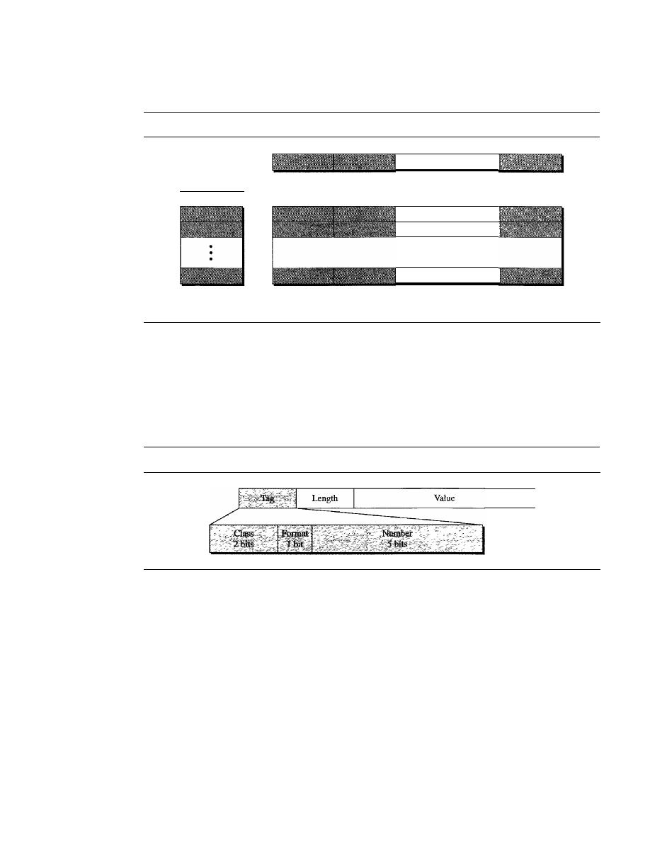
884
CHAPTER
28
NETWORK MANAGEMENT: SNMP
Figure 28.8 shows a conceptual view of data types.
Figure 28.8
Conceptual data types
-
a. Simple variable
b. Sequence of
(simple variables)
c. Sequence
d. Sequence of
(sequences)
...
...
Encoding Method
SMI uses another standard,
Basic Encoding Rules (BER),
to encode data to be trans-
mitted over the network. BER specifies that each piece of data be encoded in triplet
format: tag, length, and value, as illustrated in Figure 28.9.
Figure 28.9
Encoding format
o
Tag.
The tag is a I-byte field that defines the type of data.
It
is composed of three
subfields: class (2
bits),fonnat
(1
bit), and number (5 bits). The class subfield defines
the scope of the data. Four classes are defined: universal (00), applicationwide (01),
context-specific (10), and private (11). The universal data types are those taken from
ASN.l (INTEGER, OCTET STRING, and ObjectIdentifier). The applicationwide
data types are those added by SMI (IPAddress, Counter, Gauge, and TimeTicks). The
five context-specific data types have meanings that may change from one protocol to
another. The private data types are vendor-specific.
The format subfield indicates whether the data are simple (0) or structured
(1).
The number subfield further divides simple or structured data into subgroups. For
example, in the universal class, with simple format, INTEGER has a value of 2,
OCTET STRING has a value of 4, and so on. Table 28.2 shows the data types we
use in this chapter and their tags in binary and hexadecimal numbers.
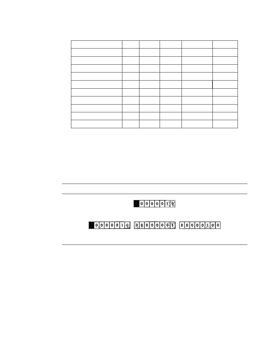
SECTION
28.2
SIMPLE NETWORK MANAGEMENT PROTOCOL (SNMP)
885
Table 28.2
Codes for data types
Data Type
Class
Format
Number
Tag (Binary)
Tag (Hex)
INTEGER
00
0
00010
00000010
02
OCTET STRING
00
0
00100
00000100
04
OBJECT IDENTIFIER
00
0
00110
00000110
06
NULL
00
0
00101
00000101
05
Sequence, sequence of
00
1
10000
00110000
30
IPAddress
01
0
00000
01000000
40
Counter
01
0
00001
01000001
41
Gauge
01
0
00010
01000010
42
TimeTicks
01
0
00011
01000011
43
Opaque
01
0
00100
01000100
44
o
Length. The length field is I or more bytes.
If
it is
1 byte, the most significant bit
must be O. The other 7 bits define the length of the data. If it is more than 1 byte,
the most significant bit of the first byte must be
1.
The other
7
bits of the first byte
define the number of bytes needed to define the length. See Figure 28.10 for a
depiction of the length field.
Figure 28.10
Length format
a. The colored part defines the length (2).
b. The shaded part dermes the length of the length (2 bytes);
the colored bytes define the length (260 bytes).
o
Value. The value field codes the value of the data according to the rules defined
in BER.
To show how these three fields-tag, length, and value-can define objects, we give
some examples.
Example 28.1
Figure 28.11 shows how to define INTEGER 14.
Example 28.2
Figure 28.12 shows how to define the OCTET STRING "HI."
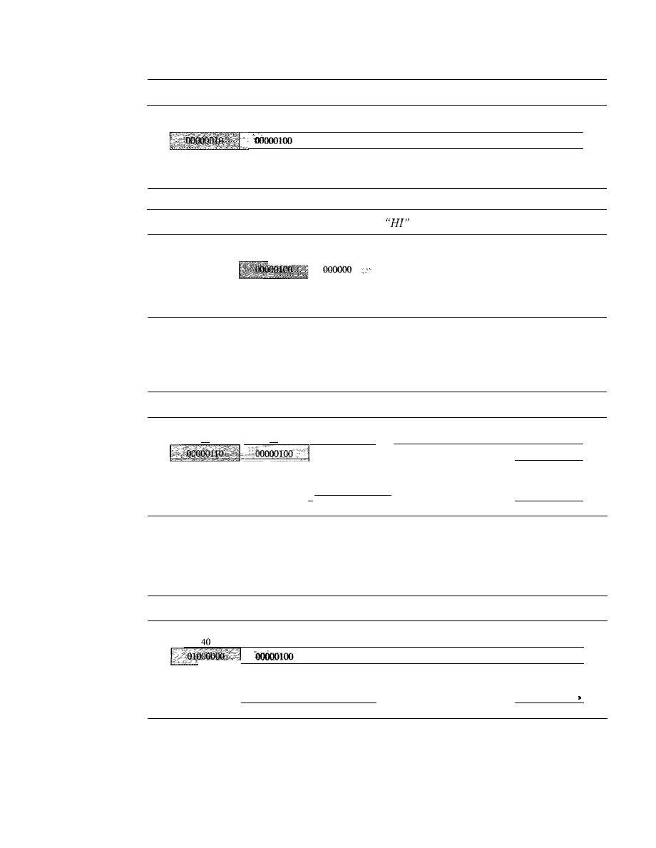
886
CHAPTER 28
NETWORK MANAGEMENT: SNMP
Figure 28.11
Example 28.1, INTEGER 14
Value (14)
02
Tag
(integer)
04
Length
(4 bytes)
00
00000000
00
00000000
00
00000000
OE
00001110
Figure 28.12
Example 28.2, OCTET STRING
04
02
48
49
10
01001000
01001001
Tag
Length
Value
Value
(String)
(2 bytes)
(H)
(1)
Example 28.3
Figure 28.13 shows how to define ObjectIdentifier 1.3.6.1 (iso.org.dod.internet).
Figure 28.13
Example 28.3, ObjectIdentifier 1.3.6.1
06
04
Tag
Length
(ObjectId)
(4 bytes)
I-
01
00000001
Value
(1)
03
06
01
00000011
00000110
00000001
Value
Value
Value
(3)
(6)
0)
1.3.6.1 (iso.org.dod.intemet)
'I
Example 28.4
Figure 28.14 shows how to define IPAddress 131.21.14.8.
Figure 28.14
Example 28.4, IPAddress 131.21.14.8
04
83
15
OE
08
10000011
00010101
00001110
00001000
Tag
Length
Value
Value
Value
Value
(IPAddress)
(4 bytes)
(131)
(21)
(14)
(8)
I-
131.21.14.8
I
Management Information Base (MIB)
The Management Information Base, version 2 (MIB2) is the second component used in
network management. Each agent has its own MIB2, which is a collection of all the
objects that the manager can manage. The objects in MIB2 are categorized under 10
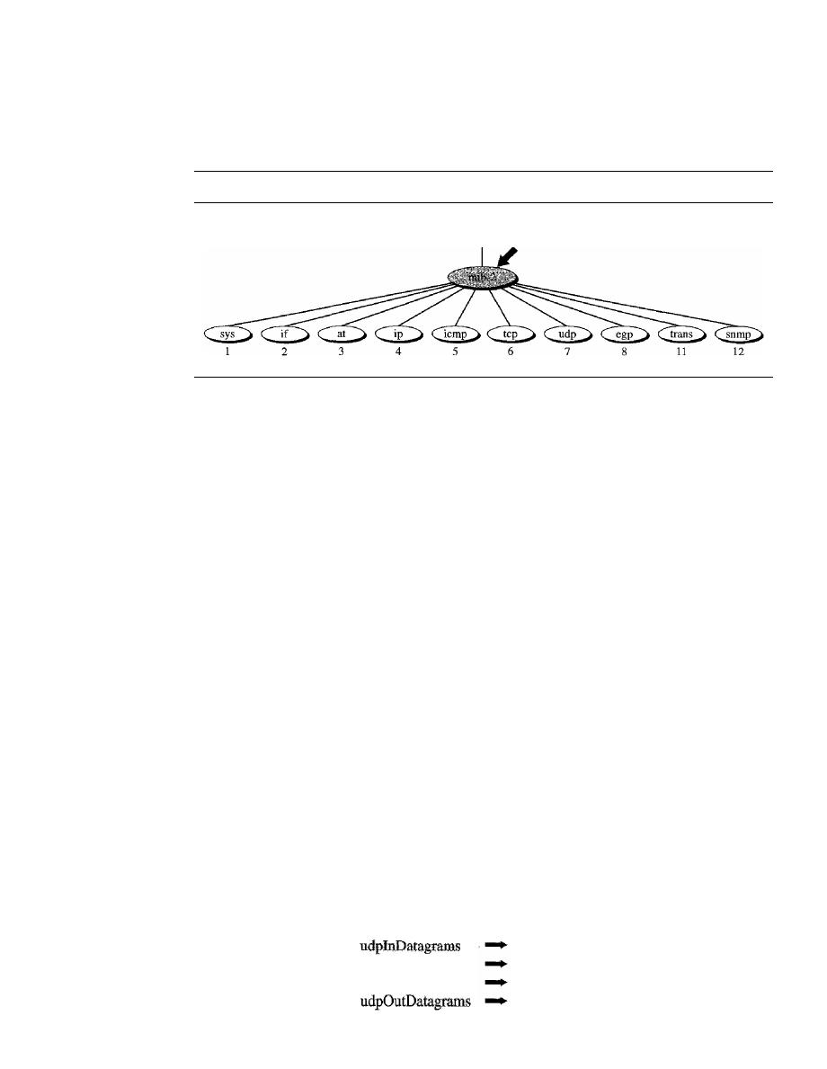
SECTION
28.2
SIMPLE NETWORK MANAGEMENT PROTOCOL (SNMP)
887
different groups: system, interface, address translation, ip, icmp, tcp, udp, egp, trans-
mission, and snmp. These groups are under the mib-2 object in the object identifier tree
(see Figure 28.15). Each group has defined variables and/or tables.
Figure 28.15
mib-2
1.3.6.1.2.1
The following is a brief description of some of the objects:
D
sys
This object
(system) defines general information about the node (system),
such as the name, location, and lifetime.
D
if
This object
(inteiface) defines information about all the interfaces of the node
including interface number, physical address, and IP address.
D
at
This object
(address translation) defines the information about the ARP table.
D
ip
This object defines information related to IP, such as the routing table and the
IP address.
D
icmp
This object defines information related
to
ICMP, such as the number of
packets sent and received and total errors created.
D
tcp
This object defines general information related to TCP, such as the connection
table, time-out value, number of ports, and number of packets sent and received.
D
udp
This object defines general information related to UDP, such as the number
of ports and number of packets sent and received.
D
snmp
This object defines general information related to SNMP itself.
Accessing MIB Variables
To show how to access different variables, we use the udp group as an example. There
are four simple variables in the udp group and one sequence of (table of) records.
Figure 28.16 shows the variables and the table.
We will show how to access each entity.
Simple Variables
To access any of the simple variables, we use the id of the group
(1.3.6.1.2.1.7) followed by the id of the variable. The following shows how to access
each variable.
. udpNoPorts
udplnErrors
1.3,6.1.2.1.7.1
1.3.6.1.2.1.7.2
1.3.6.1.2.1.7.3
1.3.6.1.2.1.7.4
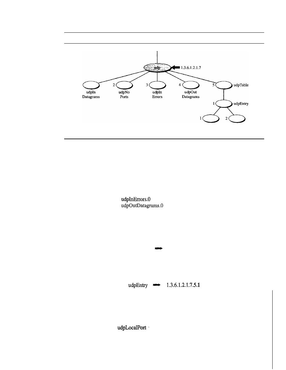
888
CHAPTER
28
NETWORK MANAGEMENT: SNMP
Figure 28.16
udp group
udpLocal
Address
udpLocal
Port
However, these object identifiers define the variable, not the instance (contents). To show
the instance or the contents of each variable, we must add
an
instance suffix. The instance
suffix for a simple variable is simply a
O. In other words, to show an instance of the above
variables, we use the following:
udpInDatagrams.O
1.3.6.1.2.1.7.1.0
udpNoPorts.O
1.3.6.1.2.1.7.2.0
1.3.6.1.2.1.7.3.0
1.3.6.1.2.1.7.4.0
Tables
To identify a table, we first use the table id. The udp group has only one table
(with id 5) as illustrated in Figure 28.17.
So to access the table, we use the following:
udpTable
1.3.6.1.2.1.7.5
However, the table is not at the leaf level in the tree structure. We cannot access the
table; we define the entry (sequence) in the table (with id of 1), as follows:
This entry is also not a leaf and we cannot access it. We need to define each entity
(field) in the entry.
udpLocalAddress
1.3.6.1.2.1.7.5.1.1
1.3.6.1.2.1.7.5.1.2
These two variables are at the leaf of the tree. Although we can access their instances,
we need to define
which instance. At any moment, the table can have several values for
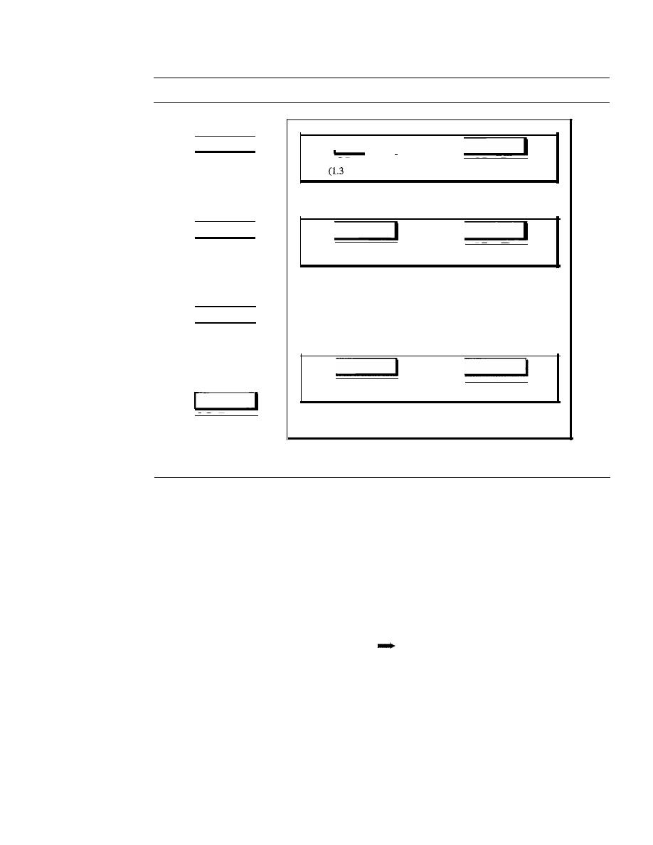
SECTION
28.2
SIMPLE NETWORK MANAGEMENT PROTOCOL (SNMP)
889
Figure 28.17
udp variables and tables
udpInDatagrams
( 1.3.6.1.2.1.7.1)
I
udpLocaIAddress
.6.1.2.1.7.5.1.1)
udpLocaIPort
(1.3.6.1.2.1.7.5.1.2)
udpEntry
(1.3.6.1.2.1.7.5.1)
udpNoPorts
(1.3.6.1.2.1.7.2)
udpLocaIAddress
(1.3.6.1.2.1.7.5.1.1)
udpLocaIPort
(1.3.6.1.2.1.7.5.1.2)
udpEntry
(1.3.6.1.2.1.7.5.1)
udpEnn-y
(1.3.6.1.2.1.7.5.1)
udplnErrors
(1.3.6.1.2.1.7.3)
udpOutDatagrams
(1.3.6.1.2.1.7.4)
udpLocalAddress
(1.3.6.1.2.1.7.5.1.1)
···
udpLocalPon
(1.3.6.1.2.1.7.5.1.2)
udpTable
(1.3.6.1.2.1.7.5)
each local address/local port pair. To access a specific instance (row) of the table, we
add the index to the above ids. In MIB, the indexes of arrays are not integers (like most
programming languages). The indexes are based on the value of one or more fields in
the entries. In our example, the udpTable is indexed based on both the local address and
the local port number. For example, Figure 28.18 shows a table with four rows and values
for each field. The index of each row is a combination of two values.
To access the instance of the local address for the first row, we use the identifier
augmented with the instance index:
udpLocalAddress.181.23.45.14.23
1.3.6.1.2.7.5.1.1.181.23.45.14.23
Note that not all tables are indexed in the same way. Some tables are indexed by using
the value of one field, others by using the value of two fields, and so on.
Lexicographic Ordering
One interesting point about the MIB variables is that the object identifiers (including
the instance identifiers) follow in lexicographic order. Tables are ordered according to
column-row rules, which means one should go column by column. In each column, one
should go from the top to the bottom, as shown in Figure 28.19.
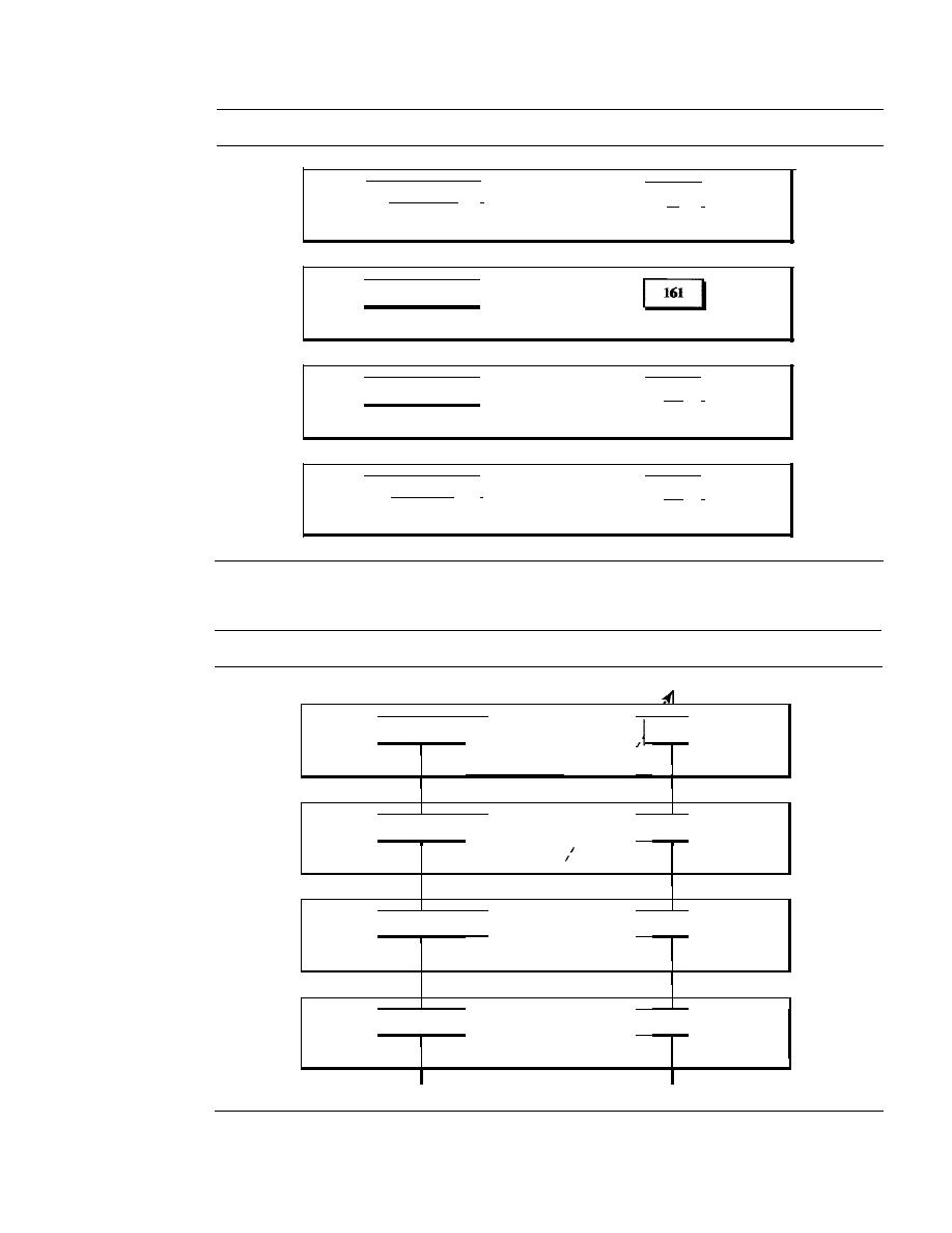
890
CHAPTER
28
NETWORK MANAGEMENT: SNMP
Figure 28.18
Indexes for udpTable
181.23.45.14
I
1.3.6.1.2.1.7.5.1.1.181.23.45.14.23
192.13.5.10
1.3.6.1.2.1.7.5.1.1.192.13.5.10.161
227.2.45.18
1.3.6.1.2.1.7.5.1.1.227.2.45.18.180
230.20.5.24
I
1.3.6.1.2.1.7.5.1.1.230.20.5.24.212
Figure 28.19
Lexicographic ordering
23
I
1.3.6.1.2.1.7.5.1.2.181.23.45.14.23
1.3.6.1.2.1.7.5.1.2.192.13.5.10.161
180
I
1.3.6.1.2.1.7.5.1.2.227.2.45.18.180
212
I
1.3.6.1.2.1.7.5.1.2.230.20.5.24.212
I
I
I
181.23.45.14
I
23
I
I
1.3.6.1.2.1.7.5.1. .181.23.45.14.23
1.3.6.1.2!1.7 .5.1. .181.23.45.14.23
I
I
I
I
I
I
I
I
I
192.13.5.10
I
161
I
I
1.3.6.1.2.1.7.5.1. .192.13.5.10.161
1.3.6.1.2.1.7.5.1. .192.13.5.10.161
I
I
I
I
I
I
I
I
I
227.2.45.18
I
180
I
I
I
1.3.6.1.2.1.7.5.1.
1.3.6.1.2.1.7.5.1. .227.2.45.18.1&0
.227.2.45.18.180
I
I
I
I
I
230.20.5.24
I
I
212
I
I
1.3.6.1.2.1.7.5.1.
1.3.6.1.2.1.7.5.1. .23tl.20.5.24.212
.230.20.5.24.212
I
I
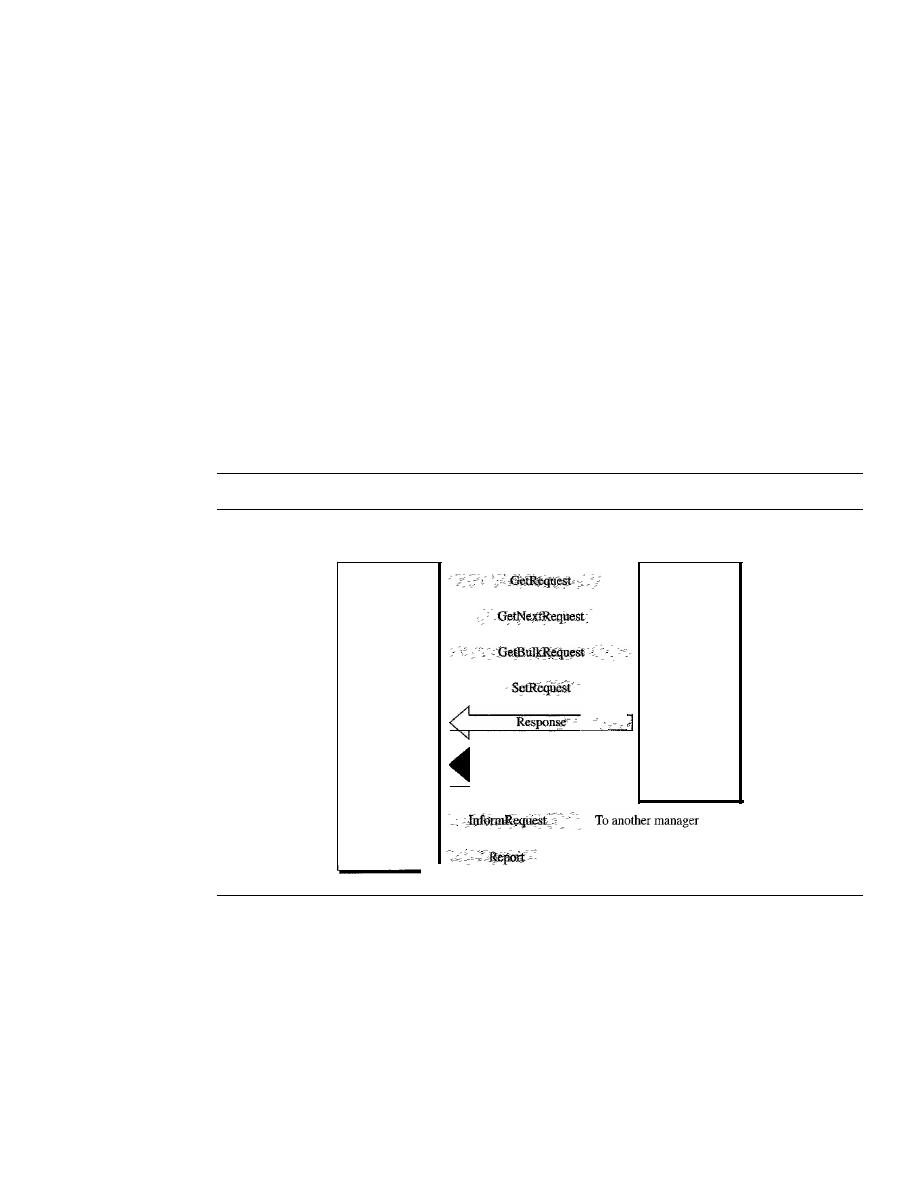
SECTION
28.2
SIMPLE NETWORK MANAGEMENT PROTOCOL (SNMP)
891
The lexicographic ordering enables a manager to access a set of variables one after
another by defining the first variable, as we will see in the GetNextRequest command in
the next section.
SNMP
SNMP uses both SMI and MIB in Internet network management.
It
is an application
program that allows
1. A manager to retrieve the value of an object defined in an agent
2. A manager to store a value in an object defined in an agent
3. An agent to send an alarm message about an abnormal situation to the manager
PDUs
SNMPv3 defines eight types of packets (or PDUs): GetRequest, GetNextRequest, Get-
BulkRequest, SetRequest, Response, Trap, InformRequest, and Report (see Figure 28.20).
Figure
28.20
SNMP PDUs
UDP
connections
Trap
SNMP
manager
Client
SNMP
agent
Server
To another manager
......
GetRequest
The GetRequest PDU is sent from the manager (client) to the agent
(server) to retrieve the value of a variable or a set of variables.
GetNextRequest
The GetNextRequest PDU is sent from the manager to the agent to
retrieve the value of a variable. The retrieved value is the value of the object following the
defined Objectid in the PDD.
It
is mostly used to retrieve the values ofthe entries
in
a table.
If
the manager does not know the indexes of the entries, it cannot retrieve the values. How-
ever, it can use GetNextRequest and define the ObjectId of the table. Because the first entry
has the ObjectId immediately after the ObjectId of the table, the value of the first entry is
returned. The manager can use this ObjectId to get the value of the next one, and so on.
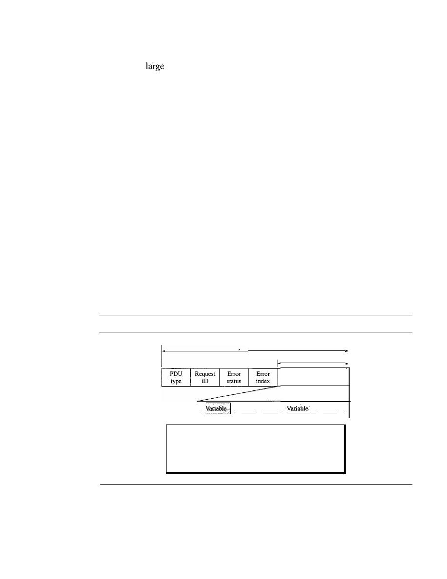
892
CHAPTER
28
NETWORK MANAGEMENT: SNMP
GetBulkRequest
The GetBulkRequest POD is sent from the manager to the agent
to retrieve a
amount of data.
It
can be used instead of multiple GetRequest and
GetNextRequest PODs.
SetRequest
The SetRequest PDD is sent from the manager to the agent to set (store)
a value in a variable.
Response
The Response PDD is sent from an agent to a manager in response to
GetRequest or GetNextRequest.
It
contains the value(s) of the variable(s) requested by
the manager.
Trap
The Trap (also called SNMPv2 Trap to distinguish it from SNMPv 1 Trap)
POD is sent from the agent to the manager to report an event. For example, if the agent
is rebooted, it infonns the manager and reports the time of rebooting.
InformRequest
The InfonnRequest POD is sent from one manager to another remote
manager to get the value of some variables from agents under the control of the remote
manager. The remote manager responds with a Response POD.
Report
The Report POD is designed to report some types of errors between managers.
It
is not yet in use.
Format
The fonnat for the eight SNMP PODs is shown in Figure 28.21. The GetBulkRequest
POD differs from the others in two areas, as shown in the figure.
Figure 28.21
SNMP PDU format
PDU
VarBind list
I
I
I
Value
I··· I
11
Value
1
Differences:
1. Error status and error index values are zeros for all request
messages except GetBulkRequest.
2. Error status field is replaced by nonrepeater field and error index
field is replaced by max-repetitions field in GetBulkRequest.
The fields are listed below:
o
PDU
type. This field defines the type of the POD (see Table 28.4).
o
Request ID. This field is a sequence number used by the manager in a Request POD
and repeated by the agent in a response.
It
is used to match a request to a response.
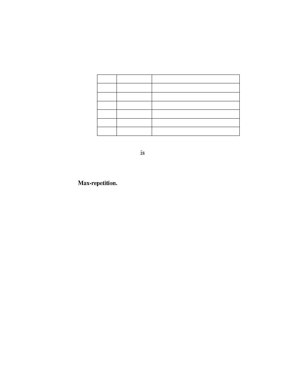
SECTION
28.2
SIMPLE NETWORK MANAGEMENT PROTOCOL (SNMP)
893
o
Error status. This is an integer that is used only in Response PDUs to show the
types of errors reported by the agent. Its value is 0 in Request PDUs. Table
28.3
lists the types of errors that can occur.
Table 28.3
Types of errors
Status
Name
Meaning
0
noError
No error
1
tooBig
Response too big to fit in one message
2
noSuchName
Variable does not exist
3
badValue
The value to be stored is invalid
4
readOnly
The value cannot be modified
5
genErr
Other errors
o
Nonrepeaters. This field
used only in GetBulkRequest and replaces the error
status field, which is empty in Request PDUs.
o
Error index. The error index is an offset that tells the manager which variable
caused the errOr.
o
This field is also used only in GetBulkRequest and replaces the
error index field, which is empty in Request PDUs.
o
VarBind list. This is a set of variables with the corresponding values the manager
wants to retrieve or set. The values are null in GetRequest and GetNextRequest. In
a Trap PDU, it shows the variables and values related to a specific PDU.
Messages
SNMP does not send only a PDU, it embeds the PDU in a message. A message in
SNMPv3 is made of four elements: version, header, security parameters, and data
(which include the encoded PDU), as shown in Figure
28.22.
Because the length of these elements is different from message to message, SNMP
uses BER to encode each element. Remember that BER uses the tag and the length to
define a value. The version defines the current version (3). The header contains values for
message identification, maximum message size (the maximum size of the reply), mes-
sage flag (one octet of data type OCTET STRING where each bit defines security type,
such as privacy or authentication, Or other information), and a message security model
(defining the security protocol). The message security parameter is used to create a mes-
sage digest (see Chapter
31).
The data contain the PDU.
If
the data are encrypted, there is
information about the encrypting engine (the manager program that did the encryption)
and the encrypting context (the type of encryption) followed by the encrypted PDU. If the
data are not encrypted, the data consist of just the PDU.
To define the type ofPDU, SNMP uses a tag. The class is context-sensitive (10), the
format is structured
(1),
and the numbers are 0,
1,2,
3, 5, 6, 7, and
8
(see Table
28.4).
Note that SNMPvl defined A4 for Trap, which is obsolete today.
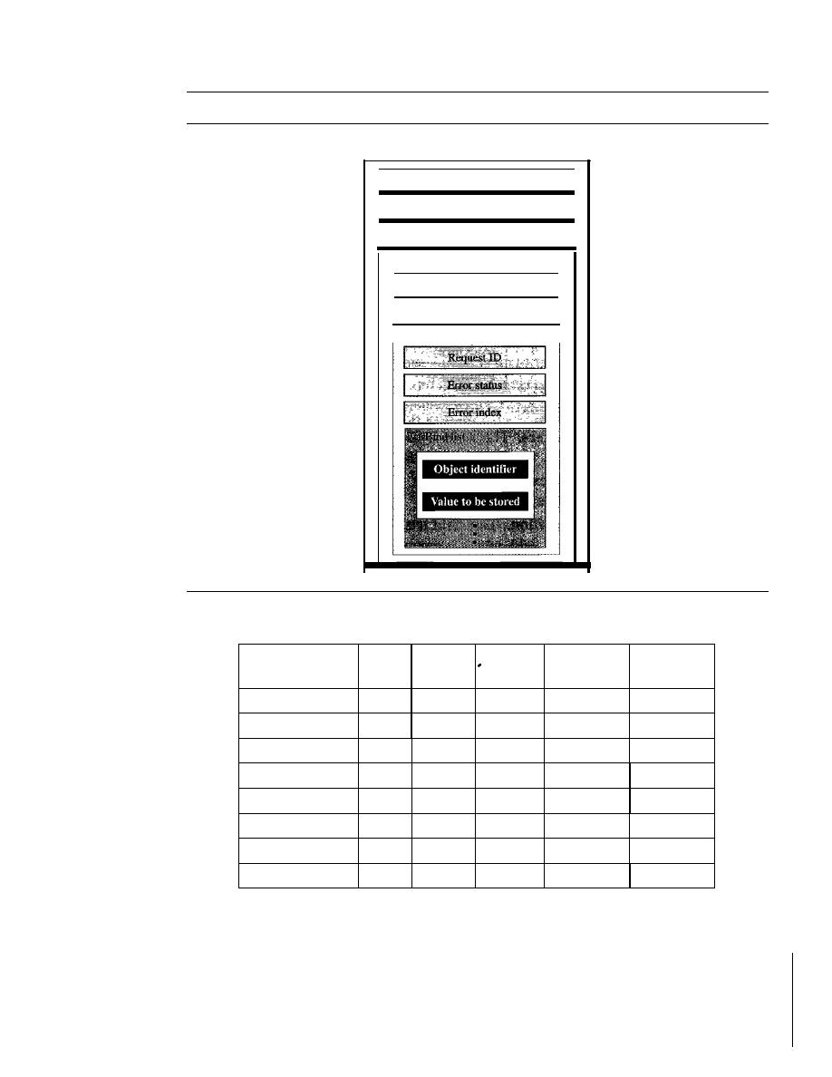
894
CHAPTER
28
NETWORK MANAGEMENT: SNMP
Figure 28.22
SNMP message
Message
Version
Header
Security parameter
Data
Context engine ID
Context name
PDU
Table 28.4
Codes for SNMP messages
Whole Tag
Whole Tag
Data
Class
Format
Number
(Binary)
(Hex)
GetRequest
10
1
00000
10100000
AO
GetNextRequest
10
1
00001
10100001
Al
Response
10
1
00010
10100010
A2
SetRequest
10
1
00011
10100011
A3
GetBulkRequest
10
1
00101
10100101
AS
InformRequest
10
1
00110
10100110
A6
Trap (SNMPv2)
10
1
00111
10100111
A7
Report
10
1
01000
10101000
A8
Example
28,5
In this example, a manager station (SNMP client) uses the GetRequest message to retrieve the
number of UDP datagrams that a router has received.
There is only one VarBind entity. The corresponding MID variable related to this informa-
tion is udpInDatagrams with the object identifier 1.3.6.1.2.1.7.1.0. The manager wants to retrieve
a value (not to store a value), so the value defines a null entity. Figure 28.23 shows the conceptual
SECTION
28.2
SIMPLE NETWORK MANAGEMENT PROTOCOL (SNMP)
895
Figure 28.23
Example 28.5
3034
020103
INTEGER, version
300C
1--
...
-
I
Header, sequence
of length 12, not shown
020140
] Two
02 02 04 00
INTEGERs
040100J
0400
Three
04 00
OCTET STRINGs
30 IF
AO 10
02
00 01 06 Il Thr
020100
ee
02 01 00
INTEGERs
Data, a
30
OF
GetRequest
sequence
PDUof
of31
30
on
length 29
bytes
VarBind
II
0609 010306 010201070100
I
Bind
list
0500
ar
Whole message
a sequence of
52 bytes
view of the packet and the hierarchical nature of sequences. We have used white and colored boxes
for the sequences and a gray one for the PDU.
The VarBind list has only one VarBind. The variable is of type 06 and length 09. The value is
of type 05 and length 00. The whole VarBind is a sequence of length OD (13). The VarBind list is
also a sequence of length OF (15). The GetRequest PDU is of length ID (29).
Now we have three OCTET STRINGs related to the security parameter, security model, and
flags. Then we have two integers defining maximum size (1024) and message ID (64). The
header is a sequence of length 12, which we left blank for simplicity. There is one integer, version
(version 3). The whole message is a sequence of 52 bytes.
Figure 28.24 shows the actual message sent by the manager station (client) to the agent (server).
UDPPorts
SNMP uses the services of UDP on two well-known ports, 161 and 162. The well-
known port 161 is used by the server (agent), and the well-known port 162 is used by
the client (manager).
The agent (server) issues a passive open on port 161.
It
then waits for a connection
from a manager (client). A manager (client) issues an active open, using an ephemeral
port, The request messages are sent from the client to the server, using the ephemeral
port as the source port and the well-known port 161 as the destination port. The
response messages are sent from the server to the client, using the well-known port 161
as the source port and the ephemeral port as the destination port.
The manager (client) issues a passive open on port 162. It then waits for a connec-
tion from an agent (server). Whenever it has a Trap message to send, an agent (server)
issues an active open, using an ephemeral port. This connection is only one-way, from
the server to the client (see Figure 28.25).
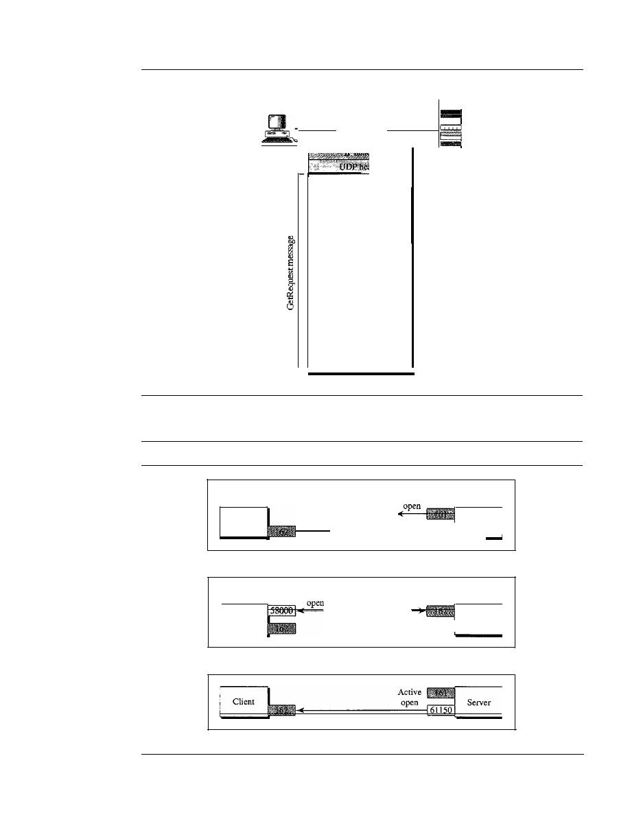
896
CHAPTER
28
NETWORK MANAGEMENT: SNMP
Figure 28.24
GetRequest message
Packet
Manager
Agent
30
34
02
01
03
30
OC
02
01
40
02
02
04
00
04
01
00
04
00
04
00
30
IF
AO
10
02
04
00
01
06
11
02
01
00
02
01
00
30
OF
30
00
06
09
01
03
06
01
02
01
07
01
00
05
00
Figure 28.25
Port numbers for SNMP
Client
Passive
open
Passive
I
Server
-_
a. Passive open by both client and server
Active
Client
I
Server
- - -
b. Exchange of request and response messages
c. Server sends trap message

SECTION
28.4
KEY TERMS
897
The client/server mechanism in SNMP is different from other protocols. Here both
the client and the server use well-known ports. In addition, both the client and the
server are running infinitely. The reason is that request messages are initiated by a man-
ager (client), but Trap messages are initiated by an agent (server).
Security
The main difference between SNMPv3 and SNMPv2 is the enhanced security. SNMPv3
provides two types of security: general and specific. SNMPv3 provides message authenti-
cation, privacy, and manager authorization. We discuss these three aspects in Chapter 31.
In
addition, SNMPv3 allows a manager to remotely change the security configuration, which
means that the manager does not have to be physically present at the manager station.
28.3
RECOMMENDED READING
For more details about subjects discussed in this chapter, we recommend the following
books and sites. The items in brackets [...] refer to the reference list at the end ofthe text.
Books
SNMP is discussed in [MS01], Chapter 25 of [Ste94], Section 22.3 of [Sta04], and
Chapter 39 of [Com04]. Network management is discussed in [Sub01].
Sites
The following sites are related to topics discussed in this chapter.
o
www.ietf.org/rfc.html Information about RFCs
RFCs
The following RFCs are related to SNMP, MIB, and SMI:
1065, 1067,1098, 1155,1157, 1212, 1213, 1229, 1231, 1243, 1284, 1351, 1352,1354, 1389,
1398, 1414, 1441, 1442, 1443, 1444,1445, 1446, 1447, 1448, 1449, 1450, 1451, 1452, 1461,
1472, 1474, 1537, 1623,1643,1650, 1657, 1665, 1666, 1696, 1697, 1724, 1742,1743, 1748,
1749
28.4
KEY TERMS
Abstract Syntax Notation 1 (ASN.l)
accounting management
agent
Basic Encoding Rules (BER)
configuration management
fault management
hardware documentation
lexicographic ordering
Management Information Base (MIB)
manager
network management
object identifier
performance management
security management

898
CHAPTER
28
NE1WORK MANAGEMENT: SNMP
simple data type
Simple Network Management Protocol
(SNMP)
structured data type
Structure of Management Information
(SMI)
trap
28.5
SUMMARY
o
The five areas comprising network management are configuration management,
fault management, performance management, accounting management, and security
management.
o
Configuration management is concerned with the physical or logical changes of
network entities.
It
includes the reconfiguration and documentation of hardware,
software, and user accounts.
o
Fault management is concerned with the proper operation of each network compo-
nent. It can be reactive or proactive.
o
Performance management is concerned with the monitoring and control of the
network to ensure the network runs as efficiently as possible.
It
is quantified by
measuring the capacity, traffic, throughput, and response time.
o
Security management is concerned with controlling access to the network.
o
Accounting management is concerned with the control of user access to network
resources through charges.
o
Simple Network Management Protocol (SNMP) is a framework for managing
devices in an internet using the TCP/IP protocol suite.
o
A manager, usually a host, controls and monitors a set of agents, usually routers.
o
The manager is a host that runs the SNMP client program.
o
The agent is a router or host that runs the SNMP server program.
o
SNMP frees management tasks from both the physical characteristics of the managed
devices and the underlying networking technology.
o
SNMP uses the services of two other protocols: Structure of Management Infor-
mation (SMI) and Management Information Base (MIB).
o
SMI names objects, defines the type of data that can be stored in an object, and
encodes the data.
o
SMI objects are named according to a hierarchical tree structure.
o
SMI data types are defined according to Abstract Syntax Notation 1 (ASN.l).
o
SMI uses Basic Encoding Rules (BER) to encode data.
o
MIB is a collection of groups of objects that can be managed by SNMP.
o
MIB uses lexicographic ordering to manage its variables.
o
SNMP functions in three ways:
1. A manager can retrieve the value of an object defined in an agent.
2. A manager can store a value in an object defined in an agent.
3. An agent can send an alarm message to the manager.

SECTION
28.6
PRACTICE SET
899
o
SNMP defines eight types of packets: GetRequest, GetNextRequest, SetRequest,
GetBulkRequest, Trap, InformRequest, Response, and Report.
o
SNMP uses the services ofUDP on two well-known ports, 161 and 162.
o
SNMPv3 has enhanced security features over previous versions.
28.6
PRACTICE SET
Review Questions
I. Define network management.
2. List five functions of network management.
Define configuration management and its purpose.
4. List two subfunctions of configuration management.
S.
Define fault management and its purpose.
6. List two subfunctions of fault management.
7. Define performance management and its purpose.
8. List four measurable quantities of performance management.
9. Define security management and its purpose.
10. Define account management and its purpose.
Exercises
II. Show the encoding for INTEGER 1456.
12. Show the encoding for the OCTET STRING "Hello World."
13. Show the encoding for an arbitrary OCTET STRING oflength 1000.
14. Show how the following record (sequence) is encoded.
INTEGER
2345
OCTET STRING
"COMPUTER"
IP Address
185.32.1.5
15. Show how the following record (sequence) is encoded.
Time Tick
12000
INTEGER
14564
Object Id
1.3.6.1.2.1.7
16. Show how the following array (sequence of) is encoded. Each element is an
integer.
2345
1236
122
1236

900
CHAPTER
28
NETWORK MANAGEMENT: SNMP
17. Show how the following array of records (sequence of sequence) is encoded.
INTEGER
2345
1123
3456
OCTET STRING
"COMPUTER"
"DISK"
"MONITOR"
Counter
345
1430
2313
18. Decode the following.
a. 02 04 01 02 14 32
b. 30060201 11 0201 14
c.
300904034143420202 14 14
d. 30 OA 40 04 2351 6271 0202 14 12
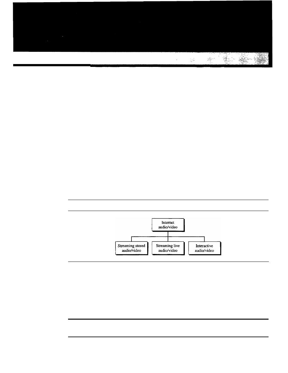
CHAPTER 29
Multimedia
Recent advances in technology have changed our use of audio and video. In the past,
we listened to an audio broadcast through a radio and watched a video program broad-
cast through a TV. We used the telephone network to interactively communicate with
another party. But times have changed. People want to use the Internet not only for text
and image communications, but also for audio and video services. In this chapter, we
concentrate on applications that use the Internet for audio and video services.
We can divide audio and video services into three broad categories: streaming
stored audio/video, streaming live audio/video, and interactive audio/video, as shown
in Figure 29.1. Streaming means a user can listen to (or watch) the file after the down-
loading has started.
Figure 29.1
Internet audio/video
In the first category, streaming stored audio/video, the files are compressed and
stored on a server. A client downloads the files through the Internet. This is sometimes
referred to as on-demand audio/video. Examples of stored audio files are songs,
symphonies, books on tape, and famous lectures. Examples of stored video files are
movies, TV shows, and music video clips.
Streaming stored audio/video refers
to
on-demand
requests for compressed audio/video files.
901

902
CHAPTER
29
MULTIMEDIA
In the second category, streaming live audio/video, a user listens to broadcast
audio and video through the Internet. A good example of this type of application is the
Internet radio. Some radio stations broadcast their programs only on the Internet; many
broadcast them both on the Internet and on the air. Internet TV is not popular yet, but
many people believe that TV stations will broadcast their programs on the Internet in
the future.
Streaming live audio/video refers to the broadcasting of
radio and TV programs through the Internet.
In the third category, interactive audio/video, people use the Internet to interactively
communicate with one another. A good example of this application is Internet telephony
and Internet teleconferencing.
Interactive audio/video refers to the use of the Internet
for interactive audio/video applications.
We will discuss these three applications in this chapter, but first we need to discuss
some other issues related to audio/video: digitizing audio and video and compressing
audio and video.
29.1
DIGITIZING AUDIO AND VIDEO
Before audio or video signals can be sent on the Internet, they need to be digitized. We
discuss audio and video separately.
Digitizing Audio
When sound is fed into a microphone, an electronic analog signal is generated which
represents the sound amplitude as a function of time. The signal is called an analog
audio signal.
An analog signal, such as audio, can be digitized to produce a digital sig-
nal. According to the Nyquist theorem, if the highest frequency of the signal is
f,
we
need to sample the signal
21
times per second. There are other methods for digitizing
an audio signal, but the principle is the same.
Voice is sampled at 8000 samples per second with 8 bits per sample. This results in
a digital signal of 64 kbps. Music is sampled at 44,100 samples per second with 16 bits
per sample. This results in a digital signal of 705.6 kbps for monaural and 1.411 Mbps
for stereo.
Digitizing Video
A video consists of a sequence of frames.
If
the frames are displayed on the screen fast
enough, we get an impression of motion. The reason is that our eyes cannot distinguish
the rapidly flashing frames as individual ones. There is no standard number of frames
per second; in North America 25 frames per second is common. However, to avoid a

SECTION
29.2
AUDIO AND VIDEO COMPRESSION
903
condition known as flickering, a frame needs to be refreshed. The TV industry repaints
each frame twice. This means 50 frames need to be sent, or if there is memory at the
sender site, 25 frames with each frame repainted from the memory.
Each frame is divided into small grids, called picture elements or pixels. For black-
and-white TV, each 8-bit pixel represents one of 256 different gray levels. For a color TV,
each pixel is 24 bits, with 8 bits for each primary color (red, green, and blue).
We can calculate the number of bits in 1 s for a specific resolution. In the lowest
resolution a color frame is made of 1024 x 768 pixels. This means that we need
2 x25 x I024x768x 24=944 Mbps
This data rate needs a very high data rate technology such as SONET. To send video
using lower-rate technologies, we need to compress the video.
Compresswn
is needed to send video over the Internet.
29.2
AUDIO AND VIDEO COMPRESSION
To send audio or video over the Internet requires compression. In this section, we discuss
audio compression first and then video compression.
Audio Compression
Audio compression can be used for speech or music. For speech, we need to compress
a 64-kHz digitized signal; for music, we need to compress a 1.41 I-MHz signal. Two
categories of techniques are used for audio compression: predictive encoding and
perceptual encoding.
Predictive Encoding
In predictive encoding, the differences between the samples are encoded instead of
encoding all the sampled values. This type of compression is normally used for speech.
Several standards have been defined such as GSM (13 kbps), G.729 (8 kbps), and
G.723.3 (6.4 or 5.3 kbps). Detailed discussions of these techniques are beyond the
scope of this book.
Perceptual Encoding: MP3
The most common compression technique that is used to create CD-quality audio is
based on the perceptual encoding technique. As we mentioned before, this type of
audio needs at least 1.411 Mbps; this cannot be sent over the
without compres-
sion.
MP3 (MPEG audio layer 3), a part of the MPEG standard (discussed in the video
compression section), uses this technique.
Perceptual encoding is based on the science of psychoacoustics, which is the study
of how people perceive sound. The idea is based on flaws in our auditory system:
Some sounds can mask other sounds. Masking can happen in frequency and time. In
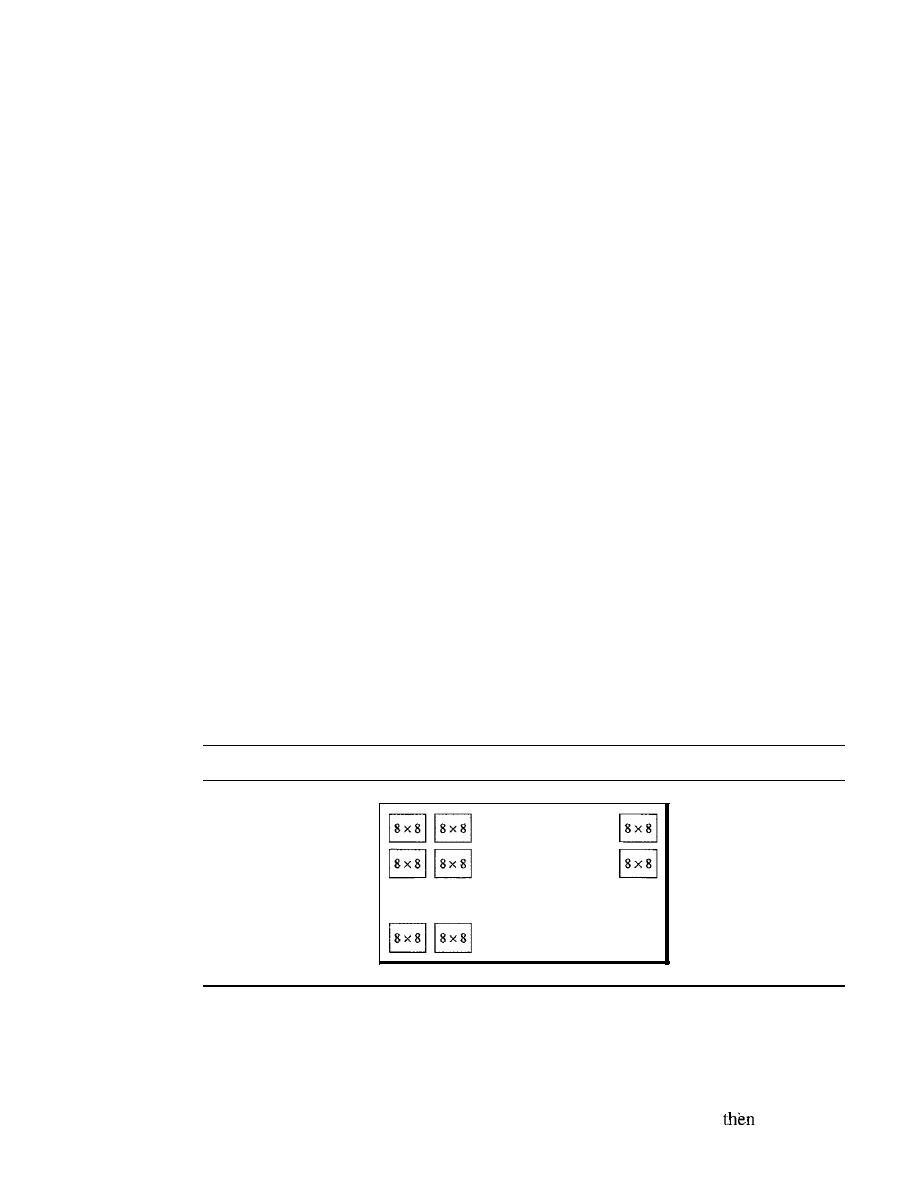
904
CHAPTER
29
MULTIMEDIA
frequency masking, a loud sound in a frequency range can partially or totally mask a
softer sound in another frequency range. For example, we cannot hear what our dance
partner says in a room where a loud heavy metal band is performing. In temporal
masking, a loud sound can numb our ears for a short time even after the sound has
stopped.
MP3 uses these two phenomena, frequency and temporal masking, to compress
audio signals. The technique analyzes and divides the spectrum into several groups.
Zero bits are allocated to the frequency ranges that are totally masked. A small number
of bits are allocated to the frequency ranges that are partially masked. A larger number of
bits are allocated to the frequency ranges that are not masked.
MP3 produces three data rates: 96 kbps, 128 kbps, and 160 kbps. The rate is based
on the range of the frequencies in the original analog audio.
Video Compression
As we mentioned before, video is composed of multiple frames. Each frame is one
image. We can compress video by first compressing images. Two standards are prevalent
in the market. Joint Photographic Experts Group (JPEG) is used to compress images.
Moving Picture Experts Group (MPEG) is used to compress video. We briefly discuss
JPEG and then MPEG.
Image Compression: lPEG
As we discussed previously, if the picture is not in color (gray scale), each pixel can be
represented by an 8-bit integer (256 levels).
If
the picture is in color, each pixel can
be represented by 24 bits (3 x 8 bits), with each 8 bits representing red, blue, or green
(RBG). To simplify the discussion, we concentrate on a gray scale picture.
In JPEG, a gray scale picture is divided into blocks of 8 x 8 pixels (see Figure 29.2).
Figure 29.2
lPEG
gray
scale
..
The purpose of dividing the picture into blocks is to decrease the number of calcula-
tions because, as you will see shortly, the number of mathematical operations for each
picture is the square of the number of units.
The whole idea of JPEG is to change the picture into a linear (vector) set of numbers
that reveals the redundancies. The redundancies (lack of changes) can
be removed
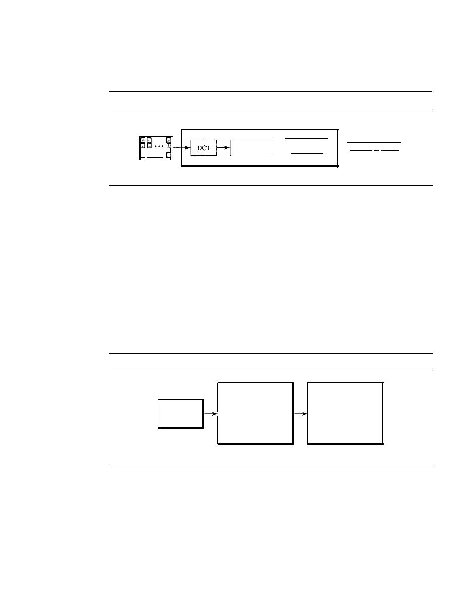
SECTION
29.2
AUDIO AND VIDEO COMPRESSION
905
by using one of the text compression methods. A simplified scheme of the process is
shown in Figure 29.3.
Figure 29.3
lPEG process
Three phases of JPEG
•••
o
D···
Blocked
image
Quantization
Data
compression
001111· .. 000001
Compressed
image
Discrete Cosine Transform (DCT)
In this step, each block of 64 pixels goes through
a transformation called the discrete cosine transform (DCT). The transformation
changes the 64 values so that the relative relationships between pixels are kept but the
redundancies are revealed. We do not give the formula here, but we do show the results
of the transformation for three cases.
Case 1
In this case, we have a block of uniform gray, and the value of each pixel is
20. When we do the transformations, we get a nonzero value for the first element
(upper left comer); the rest of the pixels have a value of O. The value of
T(O,O)
is the
average (multiplied by a constant) of the
P(x,y)
values and is called the
de value
(direct
current, borrowed from electrical engineering). The rest of the values, called
ae values,
in
T(m,n)
represent changes in the pixel values. But because there are no changes, the
rest of the values are Os (see Figure 29.4).
Figure 29.4
Case
1:
uniform
gray
scale
20 20 20 20 20 20 20 20
160 0 0 0 0 0 0 0
20 20 20 20 20 20 20 20
o
0 0 0 0 0 0 0
20 20 20 20 20 20 20 20
o
0 0 0 0 0 0 0
20 20 20 20 20 20 20 20
o
0 0 0 0 0 0 0
20 20 20 20 20 20 20 20
o
0 0 0 0 0 0
0
20 20 20 20 20 20 20 20
o
0 0 0 0 0 0 0
Picture
20 20 20 20 20 20 20 20
o
0
0 0 0 0 0
0
20 20 20 20 20 20 20 20
o
0
0
0 0 0 0 0
P(X,y)
T(m,n)
Case 2
In the second case, we have a block with two different uniform gray scale sec-
tions. There is a sharp change in the values of the pixels (from 20 to 50). When we do
the transformations, we get a dc value as well as nonzero ac values. However, there are
only a few nonzero values clustered around the dc value. Most of the values are 0 (see
Figure 29.5).
Case 3
In the third case, we have a block that changes gradually. That is, there is no
sharp change between the values of neighboring pixels. When we do the transformations,
we get a de value, with many nonzero ac values also (Figure 29.6).
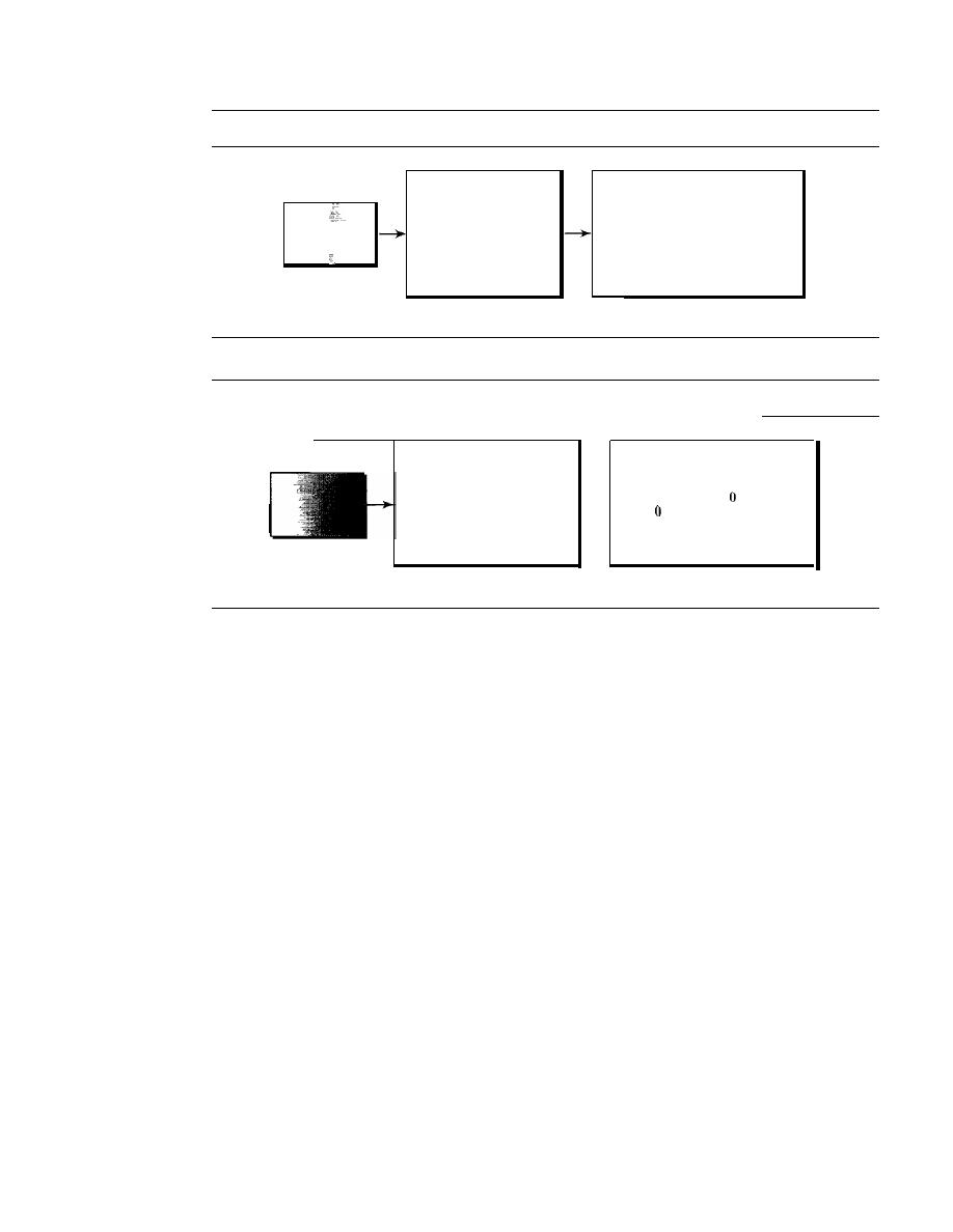
906
CHAPTER
29
MULTIMEDIA
Figure 29.5
Case
2:
two sections
20 20 20 20 50 50 50 50
280
2109 0
39
0
225
0
22
20 20 20 20 50 50 50 50
0
0
0
0
0
0
0
0
20 20 20 20 50 50 50 50
0
0
0
0
0
0
0
0
20 20 20 20 50 50 50 50
0
0
0
0
0
0
0
0
20 20 20 20 50 50 50 50
0
0
0
0
0
0
0
0
20 20 20 20 50 50 50 50
0
0
0
0
0
0
0
0
Picture
20 20 20 20 50 50 50 50
0
0
0
0
0
0
0
0
20 20 20 20 50 50 50 50
0
0
0
0
0
0
0
0
P(x,y)
T(m,n)
Figure 29.6
Case
3:
gradient gray scale
20 30 40 50 60 70 80 90
400 2146 0 231 21
3
21
28
20 30 40 50 60 70 80 90
0
0
0
0
0
0
0
0
20 30 40 50 60 70 80 90
0
0
0
0
0
0
0
0
20 30 40 50 60 70 80 90
0
0
0
0
0
0
0
20 30 40 50 60 70 80 90
0
0
0
0
0
0
0
20 30 40 50 60 70 80 90
0
0
0
0
0
0
0
0
Picture
20 30 40 50 60 70 80 90
0
0
0
0
0
0
0
0
20 30 40 50 60 70 80 90
0
0
0
0
0
0
0
0
P(x,y)
T(m,n)
From Figures 29.4,29.5, and 29.6, we can state the following:
o
The transformation creates table
T
from table
P.
o
The dc value is the average value (multiplied by a constant) of the pixels.
o
The ac values are the changes.
o
Lack of changes in neighboring pixels creates Os.
Quantization
Mter the Ttable is created, the values are quantized to reduce the num-
ber of bits needed for encoding. Previously in
quantization, we dropped the fraction
from each value and kept the integer part. Here, we divide the number by a constant and
then drop the fraction. This reduces the required number of bits even more. In most
implementations, a quantizing table (8 x 8) defines how to quantize each value. The
divisor depends on the position of the value in the
T
table. This is done to optimize the
number of bits and the number of Os for each particular application. Note that the only
phase in the process that is not reversible is the quantizing phase. We lose some infor-
mation here that is not recoverable. As a matter of fact, the only reason that lPEG is
called
lossy compression
is because of this quantization phase.
Compression
After quantization, the values are read from the table, and redundant
Os are removed. However, to cluster the Os together, the table is read diagonally in a
zigzag fashion rather than row by row or column by column. The reason is that if the
picture changes smoothly, the bottom right corner of the
T
table is all Os. Figure 29.7
shows the process.
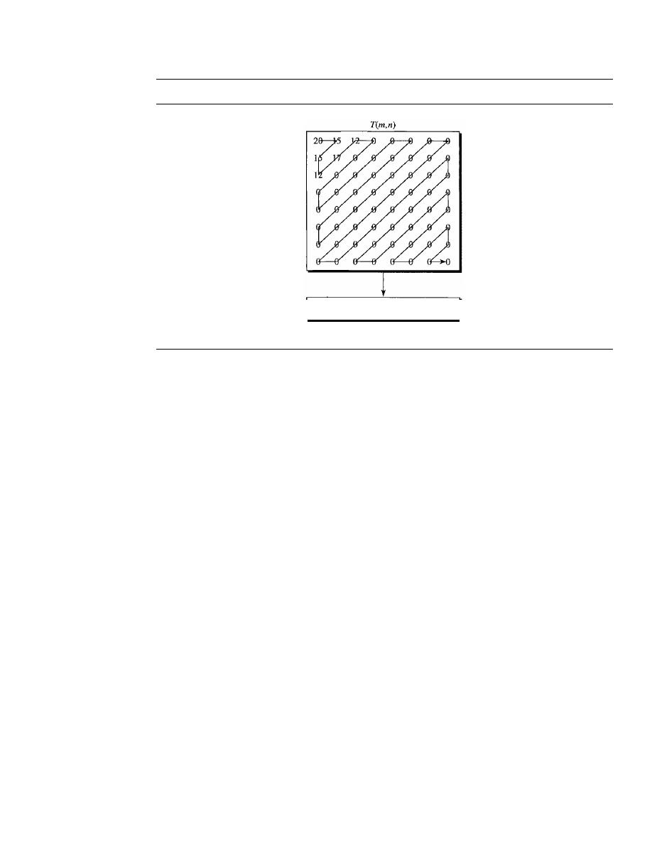
SECTION
29.2
AUDIO AND VIDEO COMPRESSION
907
Figure 29.7
Reading the table
20151512171200000"·0
Result
Video Compression: MPEG
The Moving Picture Experts Group method is used to compress video. In principle, a
motion picture is a rapid flow of a set of frames, where each frame is an image. In other
words, a frame is a spatial combination of pixels, and a video is a temporal combination
of frames that are sent one after another. Compressing video, then, means spatially com-
pressing each frame and temporally compressing a set of frames.
Spatial Compression
The spatial compression of each frame is done with IPEG (or
a modification of it). Each frame is a picture that can be independently compressed.
Temporal Compression
In temporal compression, redundant frames are removed.
When we watch television, we receive 50 frames per second. However, most of the con-
secutive frames are almost the same. For example, when someone is talking, most of the
frame is the same as the previous one except for the segment of the frame around the lips,
which changes from one frame to another.
To temporally compress data, the MPEG method first divides frames into three
categories: I-frames, P-frames, and B-frames.
o
I-frames. An intracoded frame (I-frame) is an independent frame that is not
related to any other frame (not to the frame sent before or to the frame sent after).
They are present at regular intervals (e.g., every ninth frame is an I-frame). An
I-frame must appear periodically to handle some sudden change in the frame that
the previous and following frames cannot show. Also, when a video is broadcast, a
viewer may tune in at any time.
If
there is only one I-frame at the beginning of the
broadcast, the viewer who tunes in late will not receive a complete picture.
I-frames are independent of other frames and cannot be constructed from other frames.
o
P-frames. A predicted frame (P-frame) is related to the preceding I-frame or
P-frame.
In
other words, each P-frame contains only the changes from the preceding
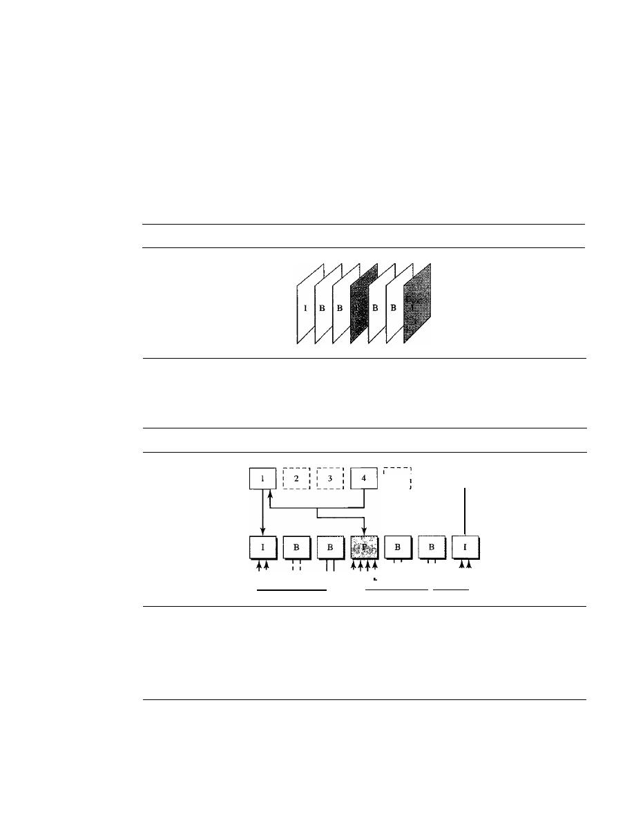
908
CHAPTER
29
MULTIMEDIA
frame. The changes, however, cannot cover a big segment. For example, for a fast-
moving object, the new changes may not be recorded in a P-frame. P-frames can be
constructed only from previous 1- or P-frames. P-frames carry much less informa-
tion than other frame types and carry even fewer bits after compression.
o
B-frames. A bidirectional frame (B.frame)
is related to the preceding and
following I-frame or P-frame. In other words, each B-frame is relative to the past
and the future. Note that a B-frame is never related to another B-frame.
Figure 29.8 shows a sample sequence of frames.
Figure 29.8
MPEG frames
Figure 29.9 shows how 1-, P-, and B-frames are constructed from a series of seven
frames.
Figure 29.9
MPEG frame construction
1----1
1
5
1 1
6
1
7
1
1
:
1 I
I
I
1
1 I
I
L
01
" " _ _ _
_ _ . I
_ _
01
L
_
MPEG has gone through two versions. MPEG1 was designed for a CD-ROM with
a data rate of 1.5 Mbps. MPEG2 was designed for high-quality DVD with a data rate of
3
to
6
Mbps.
29.3
STREAMING STORED AUDIONIDEO
Now that we have discussed digitizing and compressing audio/video, we turn our
attention to specific applications. The first is streaming stored audio and video. Down-
loading these types of files from a Web server can be different from downloading other
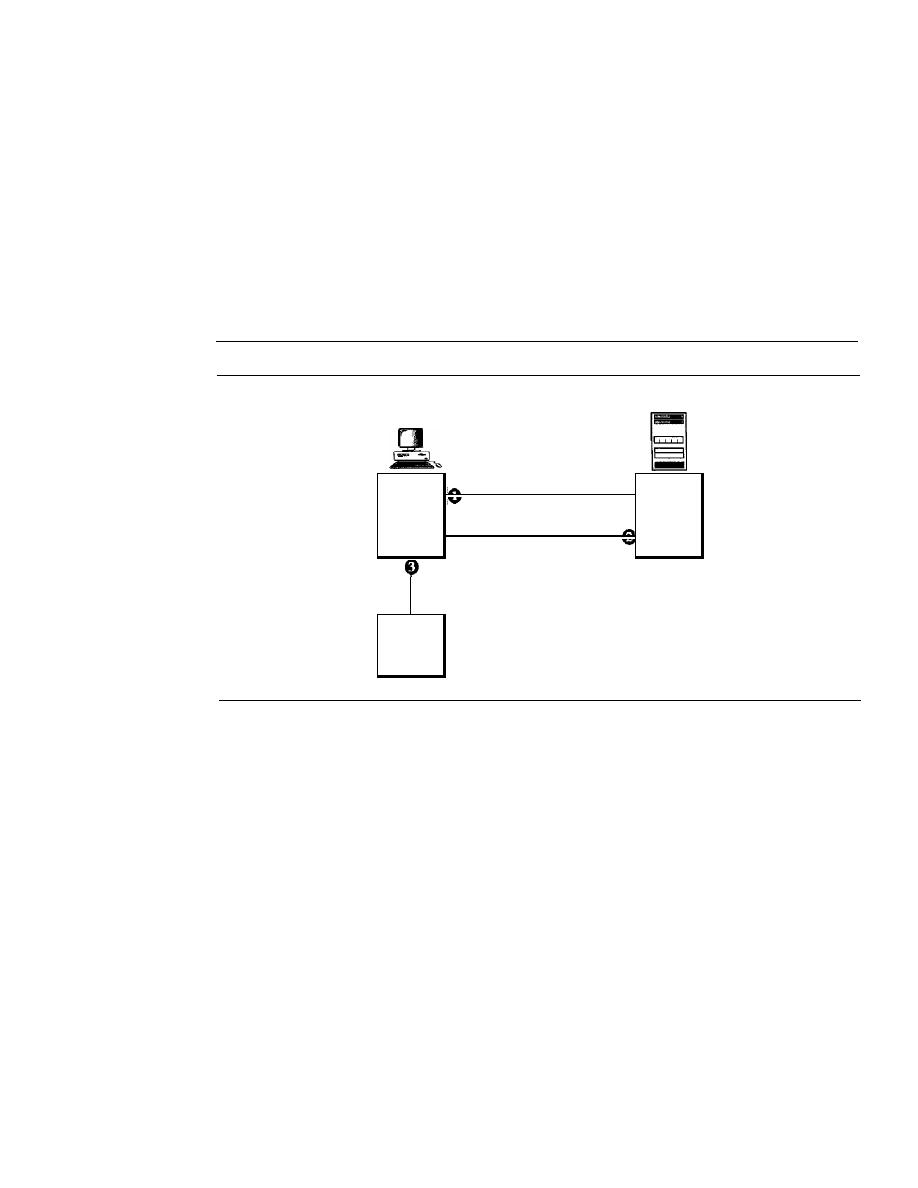
SECTION
29.3
STREAMING STORED AUDIOIVIDEO
909
types of files. To understand the concept, let us discuss four approaches, each with a
different complexity.
First Approach: Using a Web Server
A compressed audio/video file can be downloaded as a text file. The client (browser)
can use the services of HTTP and send a GET message to download the file. The Web
server can send the compressed file to the browser. The browser can then use a help
application, normally called a media player, to play the file. Figure 29.10 shows this
approach.
Figure
29.10
Using a Web server
Client machine
Server machine
GET: audio/video file
Web
Browser
RESPONSE
server
Audio/video
file
Media
player
This approach is very simple and does not involve
streaming.
However, it has a
drawback. An audio/video file is usually large even after compression. An audio file
may contain tens of megabits, and a video file may contain hundreds of megabits. In
this approach, the file needs to download completely before it can be played. Using
contemporary data rates, the user needs some seconds or tens of seconds before the file
can be played.
Second Approach: Using a Web Server with Metafile
In another approach, the media player is directly connected to the Web server for down-
loading the audio/video file. The Web server stores two files: the actual audio/video file
and a metafile that holds information about the audio/video file. Figure 29.11 shows the
steps in this approach.
1. The HTTP client accesses the Web server by using the GET message.
2. The information about the metafile comes in the response.
3. The metafile is passed to the media player.
4. The media player uses the URL in the metafile to access the audio/video file.
5. The Web server responds.
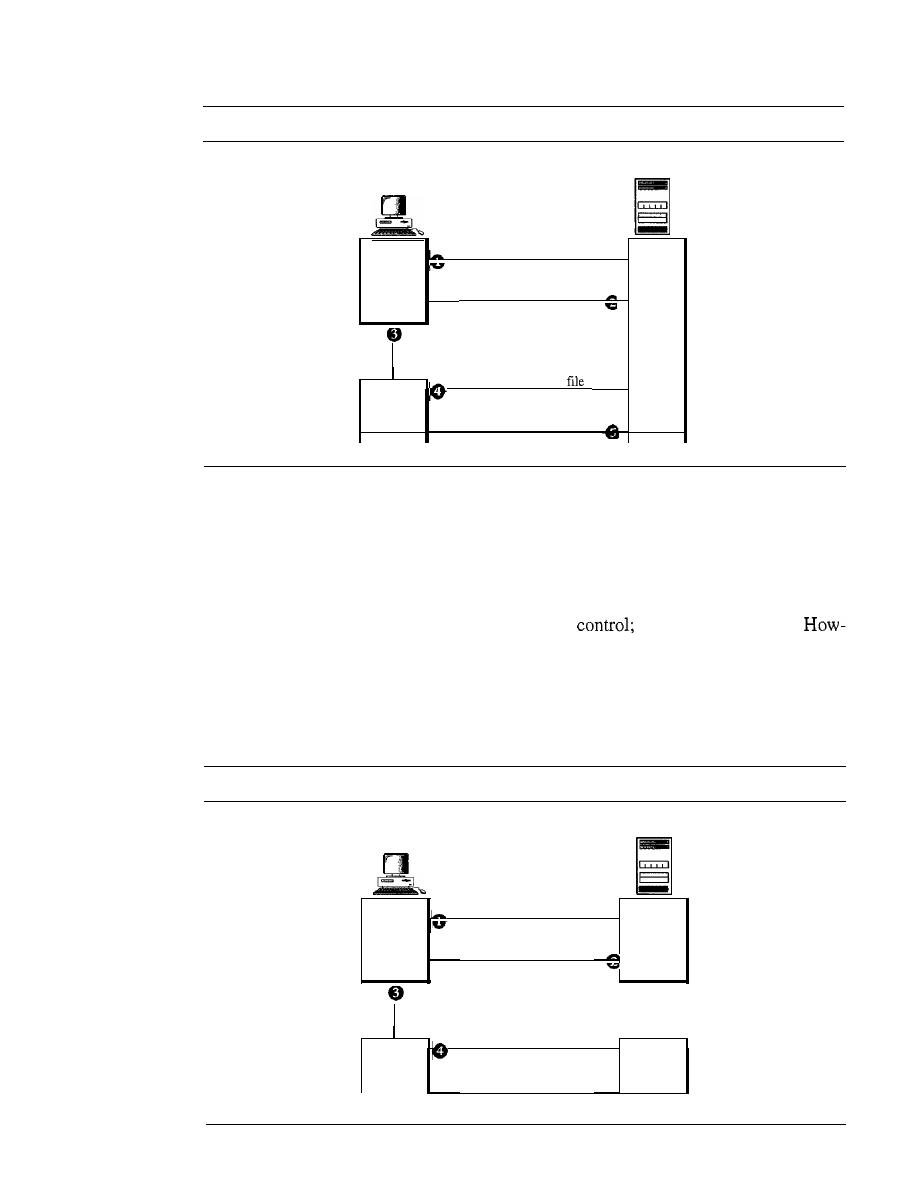
910
CHAPTER
29
MULTIMEDIA
Figure 29.11
Using a Web server with a metafile
Client machine
Server machine
GET: metafile
Browser
RESPONSE
Web
Metafile
server
GET: audio/video
Media
player
RESPONSE
Third
Approach: Using a Media Server
The problem with the second approach is that the browser and the media player both
use the services of HTIP. HTIP is designed to run over TCP. This is appropriate for
retrieving the metafile, but not for retrieving the audio/video file. The reason is that
TCP retransmits a lost or damaged segment, which is counter to the philosophy of
streaming. We need to dismiss TCP and its error
we need to use UDP.
ever, HTTP, which accesses the Web server, and the Web server itself are designed for
TCP; we need another server, a media server. Figure 29.12 shows the concept.
1.
The HTTP client accesses the Web server by using a GET message.
2. The information about the metafile comes in the response.
Figure 29.12
Using a media server
Client machine
Server machine
GET: metafile
Web
Browser
RESPONSE
server
Metafile
GET: audio/video file
Media
Media
player
RESPONSE
-
server
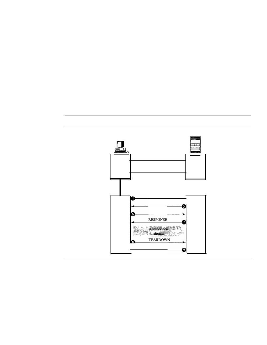
SECTION
29.3
STREAMING STORED AUDIOIVIDEO
911
3. The metafile is passed to the media player.
4. The media player uses the URL in the metafile to access the media server to down-
load the file. Downloading can take place by any protocol that uses UDP.
5. The media server responds.
Fourth Approach: Using a Media Server and RTSP
The Real-Time Streaming Protocol (RTSP) is a control protocol designed to add more
functionalities to the streaming process. Using RTSP, we can control the playing of
audio/video. RTSP is an out-of-band control protocol that is similar to the second con-
nection in FTP. Figure 29.13 shows a media server and RTSP.
Figure 29.13
Using a media server and RTSP
Client machine
GET: metafile
Browser
RESPONSE
Metafile
SETUP
RESPONSE
PLAY
Media
player
RESPONSE
Server machine
Web
server
Media
server
1.
The HTTP client accesses the Web server by using a GET message.
2. The information about the metafile comes in the response.
3. The metafile is passed to the media player.
4. The media player sends a SETUP message to create a connection with the media
server.
5. The media server responds.
6. The media player sends a PLAY message to start playing (downloading).
7. The audio/video file is downloaded by using another protocol that runs over UDP.

912
CHAPTER
29
MULTIMEDIA
8. The connection is broken by using the TEARDOWN message.
9. The media server responds.
The media player can send other types of messages. For example, a PAUSE message
temporarily stops the downloading; downloading can be resumed with a PLAY message.
29.4
STREAMING LIVE AUDIONIDEO
Streaming live audio/video is similar to the broadcasting of audio and video by radio
and TV stations. Instead of broadcasting to the air, the stations broadcast through
the Internet. There are several similarities between streaming stored audio/video and
streaming live audio/video. They are both sensitive to delay; neither can accept retrans-
mission. However, there is a difference. In the first application, the communication is
unicast and on-demand. In the second, the communication is multicast and live. Live
streaming is better suited to the multicast services of IP and the use of protocols such as
UDP and RTP (discussed later). However, presently, live streaming is still using TCP
and multiple unicasting instead of multicasting. There is still much progress to be made
in this area.
29.5
REAL-TIME INTERACTIVE AUDIONIDEO
In real-time interactive audio/video, people communicate with one another in real time.
The Internet phone or voice over IP is an example of this type of application. Video
conferencing is another example that allows people to communicate visually and orally.
Characteristics
Before addressing the protocols used in this class of applications, we discuss some
characteristics of real-time audio/video communication.
Time Relationship
Real-time data on a packet-switched network require the preservation of the time
tionship between packets of a session. For example, let us assume that a real-time video
server creates live video images and sends them online. The video is digitized and
packetized. There are only three packets, and each packet holds lOs of video informa-
tion. The first packet starts at 00:00:00, the second packet starts at 00:00: 10, and the
third packet starts at 00:00:20. Also imagine that it takes 1 s (an exaggeration for sim-
plicity) for each packet to reach the destination (equal delay). The receiver can play
back the first packet at 00:00:01, the second packet at 00:00:11, and the third packet at
00:00:21. Although there is a I-s time difference between what the server sends and
what the client sees on the computer screen, the action is happening in real time. The
time relationship between the packets is preserved. The I-s delay is not important. Fig-
ure 29.14 shows the idea.
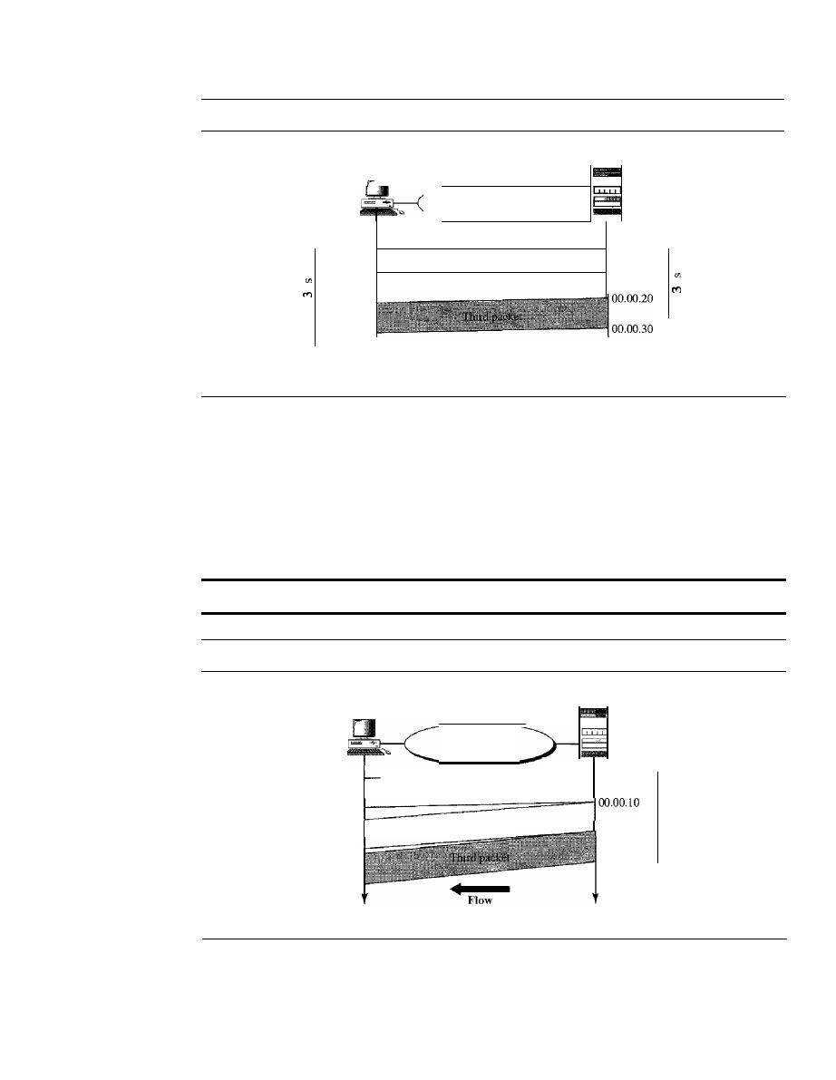
SECTION
29.5
REAL-11ME INTERACTIVE AUDIOIVIDEO
913
Figure 29.14
Time relationship
Server
Client
Internet
00.00.01
00.00.00
First packet
00.00.11
00.00.10
Second packet
0
0
00.00.21
00.00.31
Arrive and play time
Send time
But what happens if the packets arrive with different delays? For example, say the
first packet arrives at 00:00:01 (l-s delay), the second arrives at 00:00: 15 (5-s delay),
and the third arrives at 00:00:27 (7-s delay).
If
the receiver starts playing the first packet
at 00:00:01, it will finish at 00:00: 11. However, the next packet has not yet arrived; it
arrives 4 s later. There is a gap between the first and second packets and between the
second and the third as the video is viewed at the remote site. This phenomenon is called
jitter.
Figure 29.15 shows the situation.
Jitter is introduced in real-time data by the delay between packets.
Figure 29.15
Jitter
Server
Internet
Client
00.00.01
-IOO.OO.OO
First packet
00.00.30
00.00.20
Second packet
00.00.37
00.00.27
00.00.15
Arrive and play time
Send time
Timestamp
One solution to jitter is the use of a
timestamp.
If
each packet has a timestamp that
shows the time it was produced relative to the first (or previous) packet, then the receiver
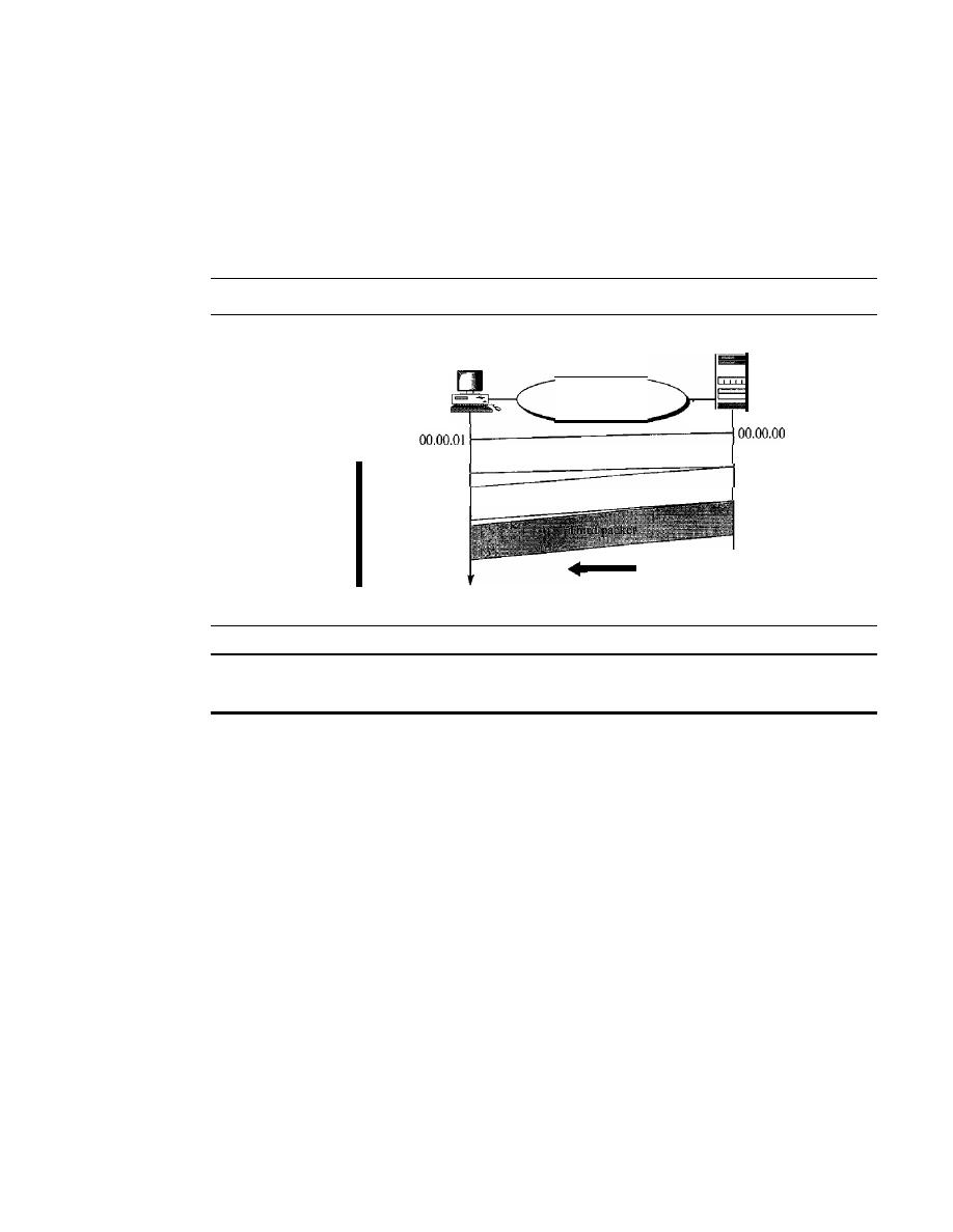
914
CHAPTER
29
MULTIMEDIA
can add this time to the time at which it starts the playback. In other words, the receiver
knows when each packet is to be played. Imagine the first packet in the previous example
has a timestamp of 0, the second has a timestamp of 10, and the third has a timestamp of
20.
If
the receiver starts playing back the first packet at 00:00:08, the second will be
played at 00:00: 18 and the third at 00:00:28. There are no gaps between the packets.
Figure 29.16 shows the situation.
Figure 29.16
Timestamp
Server
Client
Internet
First packet (0)
00.00.30
00.00.20
Flow
Second packet
(10)
00.00.37
00.00.27
00.00.10
00.00.15
00.00.28
00.00.38
00.00.18
00.00.08
Playtime
Arrive time
Send time
To prevent jitter, we can time-stamp the packets and
separate the arrival time from the playback time.
Playback Buffer
To be able to separate the arrival time from the playback time, we need a buffer to store
the data until they are played back. The buffer is referred to as a playback buffer.
When a session begins (the first bit of the first packet arrives), the receiver delays playing
the data until a threshold is reached. In the previous example, the first bit of the first
packet arrives at 00:00:01; the threshold is 7 s, and the playback time is 00:00:08. The
threshold is measured in time units of data. The replay does not start until the time units
of data are equal to the threshold value.
Data are stored in the buffer at a possibly variable rate, but they are extracted
and played back at a fixed rate. Note that the amount of data in the buffer shrinks or
expands, but as long as the delay is less than the time to play back the threshold amount
of data, there is no jitter. Figure 29.17 shows the buffer at different times for our
example.
Ordering
In addition to time relationship information and timestamps for real-time traffic, one
more feature is needed. We need a sequence number for each packet. The timestamp
alone cannot inform the receiver if a packet is lost. For example, suppose the timestamps
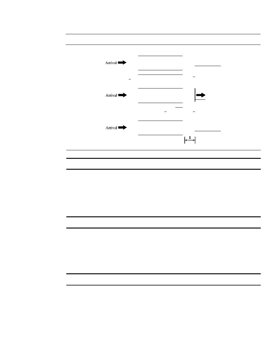
SECTION
29.5
REAL-TIME INTERACTIVE AUDIOIVIDEO
915
Figure 29.17
Playback buffer
At time 00:00:08
j"PlaYbaCk
I·
7
.[
At time 00:00:18
Playback
I·
3
·1
At time 00:00:28
I"PlaYbaCk
A playback buffer is required for real-time traffic.
are 0, 10, and 20.
If
the second packet is lost, the receiver receives just two packets with
timestamps 0 and 20. The receiver assumes that the packet with timestamp 20 is the
second packet, produced 20 s after the first. The receiver has no way of knowing that
the second packet has actually been lost. A sequence number to order the packets is
needed to handle this situation.
A sequence number on each packet
is
required for real-time traffic.
Multicasting
Multimedia playa primary role in audio and video conferencing. The traffic can be heavy,
and the data are distributed by using multicasting methods. Conferencing requires two-
way communication between receivers and senders.
Real-time traffic needs the support of multicasting.
Translation
Sometimes real-time traffic needs translation. A translator is a computer that can change
the format of a high-bandwidth video signal to a lower-quality narrow-bandwidth signal.
This is needed, for example, for a source creating a high-quality video signal at 5 Mbps
and sending to a recipient having a bandwidth of less than 1 Mbps. To receive the signal,
a translator is needed to decode the signal and encode it again at a lower quality that
needs less bandwidth.

916
CHAPTER
29
MULTIMEDIA
Translation means changing the encoding of a payload to a lower quality
to match the bandwidth of the receiving network.
Mixing
If
there is more than one source that can send data at the same time (as in a video or
audio conference), the traffic is made of multiple streams. To converge the traffic to one
stream, data from different sources can be mixed. A
mixer
mathematically adds signals
coming from different sources to create one single signal.
Mixing means combining several streams of traffic into one stream.
Support from Transport Layer Protocol
The procedures mentioned in the previous sections can be implemented in the application
layer. However, they are so common in real-time applications that implementation in the
transport layer protocol is preferable. Let's see which of the existing transport layers is
suitable for this type of traffic.
TCP is not suitable for interactive traffic. It has no provision for time-stamping, and
it does not support multicasting. However, it does provide ordering (sequence numbers).
One feature of TCP that makes it particularly unsuitable for interactive traffic is its error
control mechanism. In interactive traffic, we cannot allow the retransmission of a lost or
corrupted packet.
If
a packet is lost or corrupted in interactive traffic, it must be ignored.
Retransmission upsets the whole idea of time-stamping and playback. Today there is so
much redundancy in audio and video signals (even with compression) that we can simply
ignore a lost packet. The listener or viewer at the remote site may not even notice it.
TCP, with
all
its sophistication, is not suitable for interactive multimedia
traffic because we cannot allow retransmission of packets.
UDP is more suitable for interactive multimedia traffic. UDP supports multicasting
and has no retransmission strategy. However, UDP has no provision for time-stamping,
sequencing, or mixing. A new transport protocol, Real-time Transport Protocol (RTP),
provides these missing features.
UDP
is
more suitable than TCP for interactive traffic. However, we need the services
of RTP, another transport layer protocol, to make up for the deficiencies of UDP.
29.6
RTP
Real-time Transport Protocol (RTP)
is the protocol designed to handle real-time traffic
on the Internet. RTP does not have a delivery mechanism (multicasting, port numbers,
and so on); it must be used with UDP. RTP stands between UDP and the application
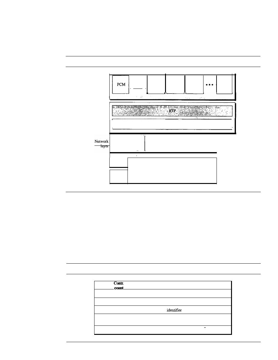
SECTION
29.6
RTP
917
program. The main contributions of RTP are time-stamping, sequencing, and mixing
facilities. Figure 29.18 shows the position ofRTP in the protocol suite.
Figure 29.18
RTP
I
Motion
IPEG
I
MPEG2
video
IP
MPEGI
video
MPEG
audio
UDP
I
Underlying LAN or WAN
technology
layer
Physical
layer
Data link
layer
Transport
layer
Application
I
H261
I
layer
RTP Packet Format
Figure 29.19 shows the format of the RTP packet header. The format is very simple
and general enough to cover all real-time applications. An application that needs
more information adds it to the beginning of its payload. A description of each field
follows.
OVer. This 2-bit field defines the version number. The current version is 2.
Figure 29.19
RTP packet header format
veri
plxl
IMI
Payload type
I
Sequence number
Time stamp
Synchronization source identifier
Contributor
·
•
•
Contributor identifier
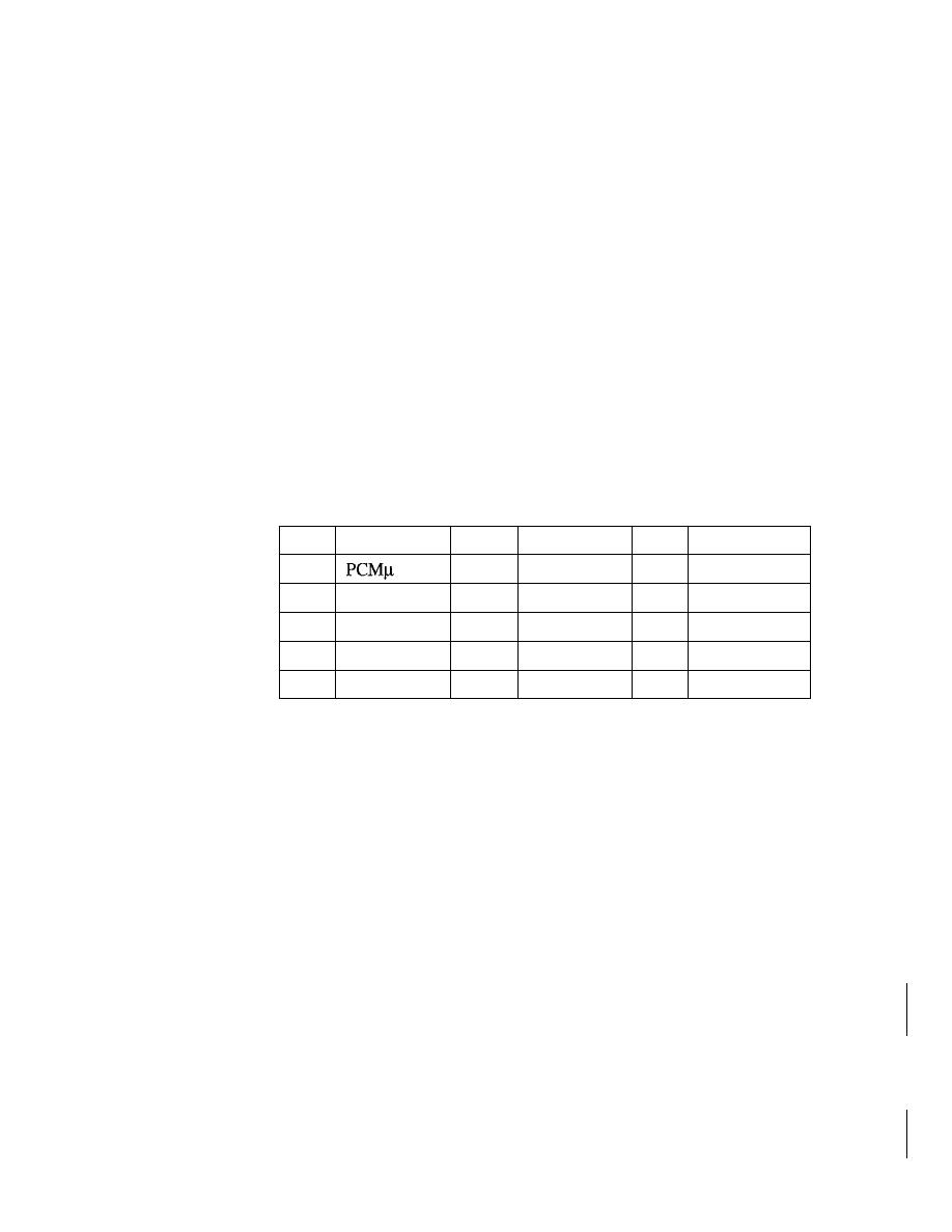
918
CHAPTER
29
MULTIMEDIA
o
P. This I-bit field, if set to 1, indicates the presence of padding at the end of the
packet. In this case, the value of the last byte in the padding defines the length of
the padding. Padding is the norm if a packet is encrypted. There is no padding if
the value of the P field is O.
o
X. This I-bit field, if set to 1, indicates an extra extension header between the
basic header and the data. There is no extra extension header if the value of this
field is O.
o
Contributor count.
This 4-bit field indicates the number of contributors. Note that
we can have a maximum of 15 contributors because a 4-bit field only allows a num-
ber between 0 and 15.
o
M. This I-bit field is a marker used by the application to indicate, for example, the
end of its data.
o
Payload type.
This 7-bit field indicates the type of the payload. Several payload
types have been defined so far. We list some common applications in Table 29.1.
A discussion of the types is beyond the scope of this book.
Table 29.1
Payload types
Type
Application
Type
Application
Type
Application
a
Audio
7
LPC audio
15
G728 audio
1
1016
8
PCMA audio
26
Motion JPEG
2
G721 audio
9
G722 audio
31
H.261
3
GSM audio
10-11
L16 audio
32
MPEGI video
5-6
DV14 audio
14
MPEGaudio
33
MPEG2 video
o
Sequence number.
This field is 16 bits in length.
It
is used to number the RTP
packets. The sequence number of the first packet is chosen randomly; it is incre-
mented by 1 for each subsequent packet. The sequence number is used by the
receiver to detect lost or out-of-order packets.
o
Timestamp.
This is a 32-bit field that indicates the time relationship between
packets. The timestamp for the first packet is a random number. For each succeeding
packet, the value is the sum of the preceding timestamp plus the time the first byte
is produced (sampled). The value of the clock tick depends on the application. For
example, audio applications normally generate chunks of 160 bytes; the clock tick
for this application is 160. The timestamp for this application increases 160 for
each RTP packet.
o
Synchronization source identifier.
If
there is only one source, this 32-bit field
defines the source. However, if there are several sources, the mixer is the synchroni-
zation source and the other sources are contributors. The value of the source identifier
is a random number chosen by the source. The protocol provides a strategy in case of
conflict (two sources start with the same sequence number).
o
Contributor identifier.
Each of these 32-bit identifiers (a maximum of 15) defines
a source. When there is more than one source in a session, the mixer is the synchro-
nization source and the remaining sources are the contributors.
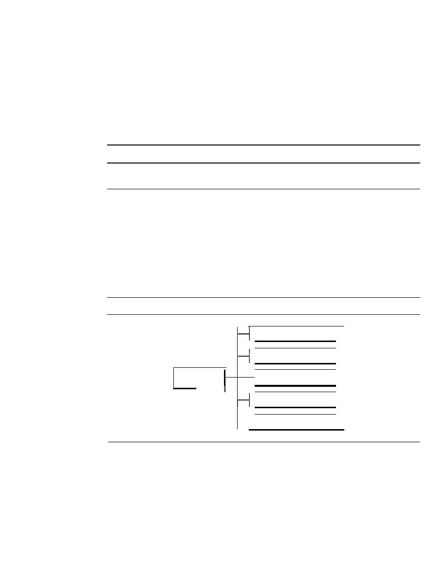
SECTION
29. 7
RTCP
919
UDPPort
Although RTP is itself a transport layer protocol, the RTP packet is not encapsulated
directly in an IP datagram. Instead, RTP is treated as an application program and is
encapsulated in a UDP user datagram. However, unlike other application programs, no
well-known port is assigned to RTP. The port can be selected on demand with only one
restriction: The port number must be an even number. The next number (an odd number)
is used by the companion of RTP, Real-time Transport Control Protocol (RTCP).
RTP uses a temporary even-numbered UDP port.
29.7
RTCP
RTP allows only one type of message, one that carries data from the source to the desti-
nation. In many cases, there is a need for other messages in a session. These messages
control the flow and quality of data and allow the recipient to send feedback to the source
or sources.
Real-time Transport Control Protocol (RTCP)
is a protocol designed for
this purpose. RTCP has five types of messages, as shown in Figure 29.20. The number
next to each box defines the type of the message.
Figure 29.20
RTCP
message types
Sender report
1
200
Receiver report
1
201
RTCP
I
Source description message
1
202
message types
I
Bye message
1
203
Application-specific message
1
204
Sender Report
The sender report is sent periodically by the active senders in a conference to report
transmission and reception statistics for all RTP packets sent during the interval. The
sender report includes an absolute timestamp, which is the number of seconds
elapsed since midnight on January 1, 1970. The absolute timestamp allows the
receiver to synchronize different RTP messages.
It
is particularly important when
both audio and video are transmitted (audio and video transmissions use separate
relative timestamps).

920
CHAPTER
29
MULTIMEDIA
Receiver Report
The receiver report is for passive participants, those that do not send RTP packets. The
report infonns the sender and other receivers about the quality of service.
Source Description Message
The source periodically sends a source description message to give additional infonna-
tion about itself. This infonnation can be the name, e-mail address, telephone number,
and address of the owner or controller of the source.
Bye Message
A source sends a bye message to shut down a stream. It allows the source to announce
that it is leaving the conference. Although other sources can detect the absence of a
source, this message is a direct announcement. It is also very useful to a mixer.
Application-Specific Message
The application-specific message is a packet for an application that wants to use new
applications (not defined in the standard).
It
allows the definition of a new message
type.
UDPPort
RTCP, like RTP, does not use a well-known UDP port.
It
uses a temporary port. The
UDP port chosen must be the number immediately following the UDP port selected for
RTP.
It
must be an odd-numbered port.
RTCP uses an odd-numbered UDP port number that
follows the port number selected for
29.8
VOICE OVER IP
Let us concentrate on one real-time interactive audio/video application:
voice over IP,
or Internet telephony. The idea is to use the Internet as a telephone network with some
additional capabilities. Instead of communicating over a circuit-switched network, this
application allows communication between two parties over the packet-switched Internet.
protocols have been designed to handle this type of communication: SIP and H.323.
We briefly discuss both.
SIP
The
Session Initiation Protocol (SIP)
was designed by IETE
It
is an application layer
protocol that establishes, manages, and terminates a multimedia session (call).
It
can be
used to create two-party, multiparty, or multicast sessions. SIP is designed to be indepen-
dent of the underlying transport layer; it can run on UDP, TCP, or SCTP.
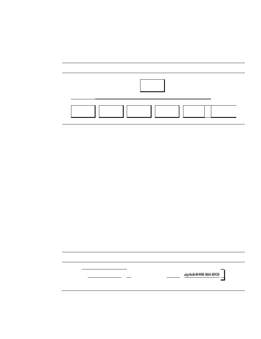
SECTION
29.8
VOICE OVER IP
921
Messages
SIP is a text-based protocol, as is HTTP. SIP, like HTTP, uses messages. Six messages
are defined, as shown in Figure 29.21.
Figure 29.21
SIP messages
SIP
messages
I
I
I
I
I
I
I
INVITE
ACK
BYE
OPTIONS
CANCEL
I
REGISTER
I
Each message has a header and a body. The header consists of several lines that
describe the structure of the message, caller's capability, media type, and so on. We
give a brief description of each message. Then we show their applications in a simple
session.
The caller initializes a session with the INVITE message. After the callee answers
the call, the caller sends an ACK message for confirmation. The BYE message termi-
nates a session. The OPTIONS message queries a machine about its capabilities. The
CANCEL message cancels an already started initialization process. The REGISTER
message makes a connection when the callee is not available.
Addresses
In a regular telephone communication, a telephone number identifies the sender, and
another telephone number identifies the receiver. SIP is very flexible. In SIP, an e-mail
address, an IP address, a telephone number, and other types of addresses can be used to
identify the sender and receiver. However, the address needs to be in SIP format (also
called
scheme).
Figure 29.22 shows some common formats.
Figure 29.22
SIP formats
sip:bob@201.23.45.78
11__
siP_:_bo_b_@_fu_da_.e_d_u_ _
11
IPv4 address
E-mail address
Phone number
Simple Session
A simple session using SIP consists of three modules: establishing, communicating, and
terminating. Figure 29.23 shows a simple session using SIP.
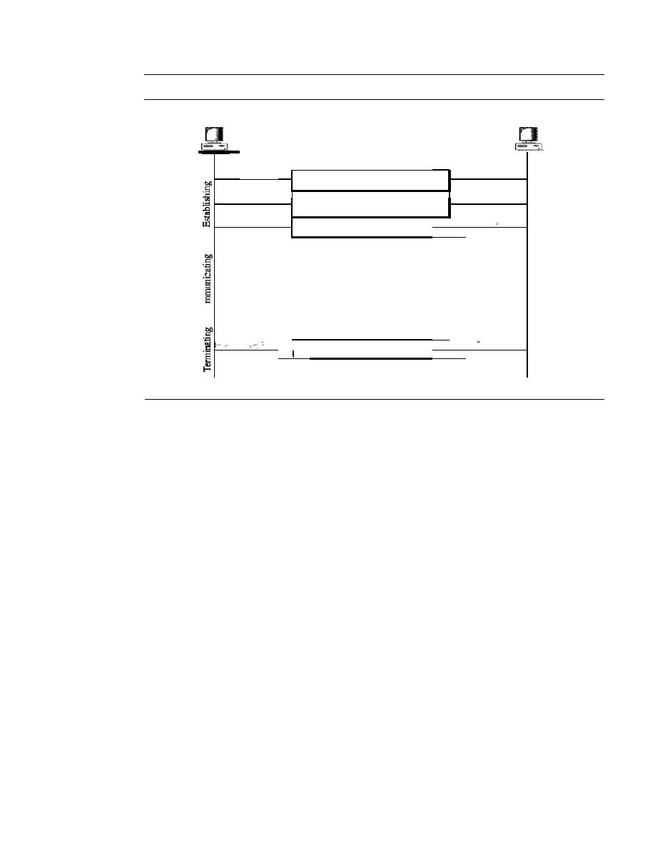
922
CHAPTER
29
MULTIMEDIA
Figure 29.23
SIP simple session
Caller
Callee
INVITE: address, options
OK: address
I
ACK
I
Exchanging audio
0
u
J
I
BYE
I
Establishing a Session
Establishing a session in SIP requires a three-way handshake.
The caller sends an INVITE message, using UDP, TCP, or SCTP to begin the communi-
cation. If the callee is willing to start the session, she sends a reply message. To confirm
that a reply code has been received, the caller sends an ACK message.
Communicating
After the session has been established, the caller and the callee can
communicate by using two temporary ports.
Terminating the Session
The session can be terminated with a BYE message sent by
either party.
Tracking the Callee
What happens if the callee is not sitting at her terminal? She may be away from her system
or at another terminal. She may not even have a fixed IP address if DHCP is being used.
SIP has a mechanism (similar to one in DNS) that finds the IP address of the terminal at
which the callee is sitting. To perform this tracking, SIP uses the concept of registration.
SIP defines some servers as registrars. At any moment a user is registered with at least one
registrar server;
this server knows the
IP
address of the callee.
When a caller needs to communicate with the callee, the caller can use the e-mail
address instead of the IP address in the INVITE message. The message goes to a proxy
server. The proxy server sends a lookup message (not part of SIP) to some registrar
server that has registered the callee. When the proxy server receives a reply message
from the registrar server, the proxy server takes the caller's INVITE message and inserts
the newly discovered IP address of the callee. This message is then sent to the callee.
Figure 29.24 shows the process.
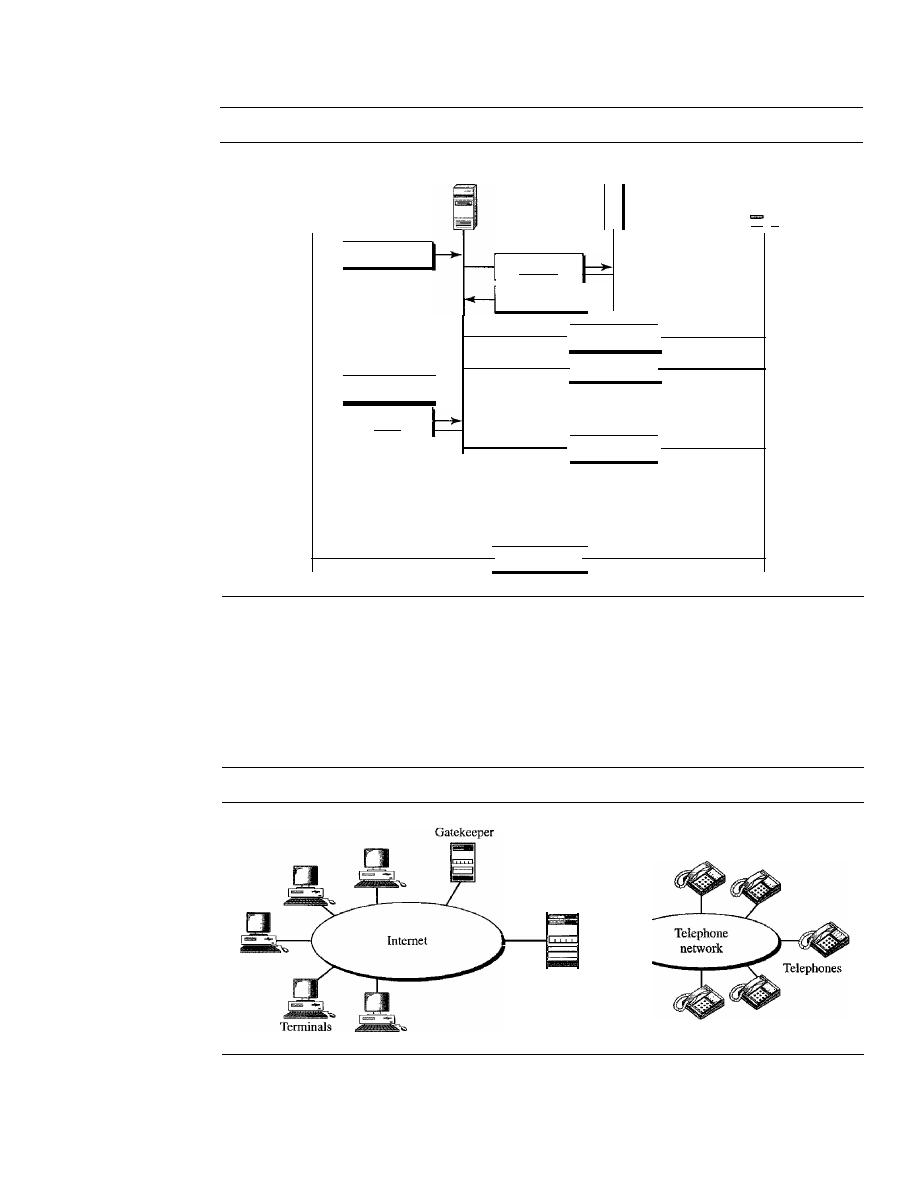
Figure 29.24
Tracking the callee
SECTION
29.8
VOICE OVER IP
923
Caller
Proxy server
INVITE
OK
ACK
Registrar
Lookup
Reply
INVITE
OK
ACK
Callee
-
Exchanging audio
BYE
H.323
H.323 is a standard designed by lTV to allow telephones on the public telephone
network to talk to computers (called
terminals
in H.323) connected to the Internet.
Figure 29.25 shows the general architecture of H.323.
Figure 29.25
H.323 architecture
Gateway
1----(
A gateway connects the Internet to the telephone network. In general, a gateway is
a five-layer device that can translate a message from one protocol stack to another. The
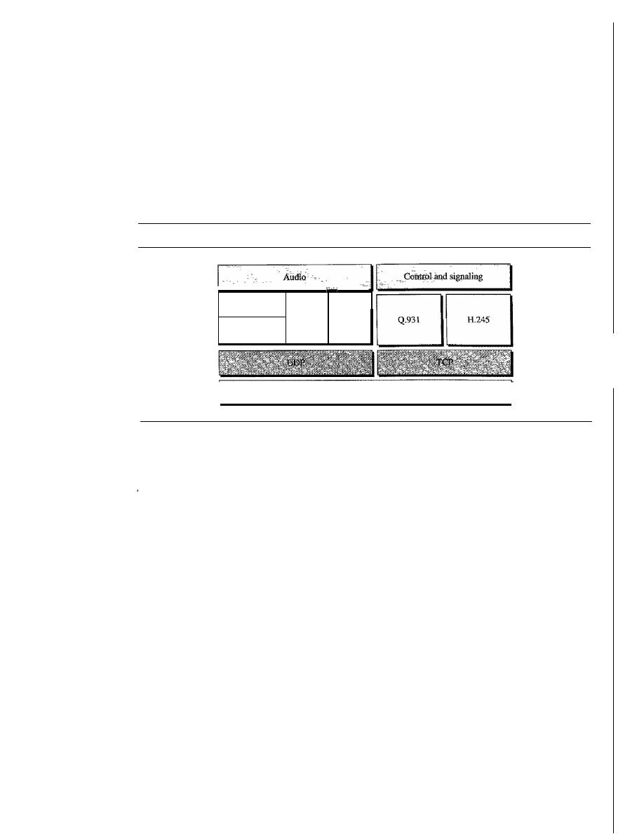
924
CHAPTER
29
MULTIMEDIA
gateway here does exactly the same thing.
It
transforms a telephone network message to
an Internet message. The gatekeeper server on the local area network plays the role of
the registrar server, as we discussed in the SIP.
Protocols
H.323 uses a number of protocols to establish and maintain voice (or video) communica-
tion. Figure 29.26 shows these protocols.
Figure 29.26
H.323 protocols
Compression
code
RTCP
H.225
RTP
IP
H.323 uses G.71 or G.723.1 for compression.
It
uses a protocol named H.245
which allows the parties to negotiate the compression method. Protocol Q.931 is used
for establishing and terminating connections. Another protocol called H.225, or RAS
(Registration!Administration!Status), is used for registration with the gatekeeper.
Operatio1l
Let us show the operation of a telephone communication using H.323 with a simple
example. Figure 29.27 shows the steps used by a terminal to communicate with a
telephone.
1. The terminal sends a broadcast message to the gatekeeper. The gatekeeper responds
with its IP address.
2. The terminal and gatekeeper communicate, using H.225 to negotiate bandwidth.
3. The terminal, gatekeeper, gateway, and telephone communicate by using Q.931 to
set up a connection.
4. The terminal, gatekeeper, gateway, and telephone communicate by using H.245 to
negotiate the compression method.
5. The terminal, gateway, and telephone exchange audio by using RTP under the
management of RTCP.
6. The terminal, gatekeeper, gateway, and telephone communicate by using Q.931 to
terminate the communication.
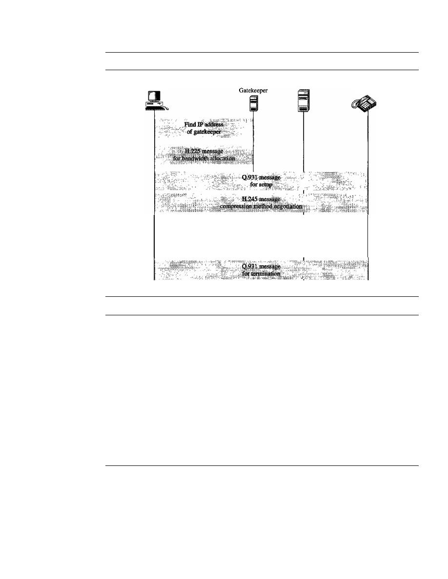
SECTION 29.10
KEY TERMS
925
Figure 29.27
H.323 example
Tenninal
RTP for audio exchange
RTCP for management
Gateway
Telephone
29.9
RECOMMENDED READING
For more details about subjects discussed in this chapter, we recommend the following
books and sites. The items in brackets [...] refer to the reference list at the end of the text.
Books
Multimedia communication is discussed in [HalOl] and in Section 7.4 of [Tan03]. Image
and video compression are fully discussed in [Dro02].
Sites
o
www.ietf.org/rfc.html
Infonnation about RFCs
29.10
KEY TERMS
bidirectional frame (B-frame)
compression
discrete cosine transform (DCT)
frequency masking
gatekeeper
gateway
H.323
interactive audio/video
intracoded frame (I-frame)
jitter

926
CHAPTER
29
MULTIMEDIA
Joint Photographic Experts Group (JPEG)
media player
media server
metafile
mixer
Moving Picture Experts Group (MPEG)
MP3
multicasting
on-demand audio/video
perceptual encoding
pixel
playback buffer
predicted frame (P-frame)
predictive encoding
quantization
Real-Time Streaming Protocol (RTSP)
real-time traffic
Real-time Transport Control Protocol
(RTCP)
Real-time Transport Protocol (RTP)
registrar server
Session Initiation Protocol (SIP)
spatial compression
streaming live audio/video
streaming stored audio/video
temporal compression
temporal masking
timestamp
translation
voice over IP
29.11
SUMMARY
o
Audio/video files can be downloaded for future use (streaming stored audio/video)
or broadcast to clients over the Internet (streaming live audio/video). The Internet
can also be used for live audio/video interaction.
o
Audio and video need to be digitized before being sent over the Internet.
o
Audio files are compressed through predictive encoding or perceptual encoding.
o
Joint Photographic Experts Group (JPEG) is a method to compress pictures and
graphics.
o
The JPEG process involves blocking, the discrete cosine transform, quantization,
and lossless compression.
o
Moving Pictures Experts Group (MPEG) is a method to compress video.
o
MPEG involves both spatial compression and temporal compression. The former
is similar to JPEG, and the latter removes redundant frames.
o
We can use a Web server, or a Web server with a metafile, or a media server, or a
media server and RTSP to download a streaming audio/video file.
o
Real-time data on a packet-switched network require the preservation of the time
relationship between packets of a session.
o
Gaps between consecutive packets at the receiver cause a phenomenon called jitter.
o
Jitter can be controlled through the use of timestamps and a judicious choice of the
playback time.
D
A playback buffer holds data until they can be played back.
D
A receiver delays playing back real-time data held in the playback buffer until a
threshold level is reached.

SECTION
29.12
PRACTICE SET
927
o
Sequence numbers on real-time data packets provide a form of error control.
o
Real-time data are multicast to receivers.
o
Real-time traffic sometimes requires a translator to change a high-bandwidth signal
to a lower-quality narrow-bandwidth signal.
o
A mixer combines signals from different sources into one signal.
o
Real-time multimedia traffic requires both UDP and Real-time Transport Protocol
(RTP).
o
RTP handles time-stamping, sequencing, and mixing.
o
Real-time Transport Control Protocol (RTCP) provides flow control, quality of data
control, and feedback to the sources.
o
Voice over IP is a real-time interactive audio/video application.
o
The Session Initiation Protocol (SIP) is an application layer protocol that establishes,
manages, and terminates multimedia sessions.
o
H.323 is an ITU standard that allows a telephone connected to a public telephone
network to talk to a computer connected to the Internet.
29.12
PRACTICE SET
Review Questions
1. How does streaming live audio/video differ from streaming stored audio/video?
2. How does frequency masking differ from temporal masking?
3. What is the function of a metafile in streaming stored audio/video?
4. What is the purpose of RTSP in streaming stored audio/video?
5. How does jitter affect real-time audio/video?
6. Discuss how SIP is used in the transmission of multimedia.
7. When would you use JPEG? When would you use MPEG?
8. In JPEG, what is the function of blocking?
9. Why is the DCT needed in JPEG?
10. What is spatial compression compared to temporal compression?
Exercises
11. In Figure 29.17 what is the amount of data in the playback buffer at each of the
following times?
a. 00:00:17
b. 00:00:20
c. 00:00:25
d. 00:00:30
12. Compare and contrast TCP with RTP. Are both doing the same thing?
13. Can we say UDP plus RTP is the same as TCP?
14. Why does RTP need the service of another protocol, RTCP, but TCP does not?

928
CHAPTER
29
MULTIMEDIA
15. In Figure 29.12, can the Web server and media server run on different machines?
16. We discuss the use of SIP in this chapter for audio. Is there any drawback to prevent
using it for video?
17. Do you think H.323 is actually the same as SIP? What are the differences? Make a
comparison between the two.
18. What are the problems for full implementation of voice over IP? Do you think we
will stop using the telephone network very soon?
19. Can
also be used for video?
Research Activities
20. Find the format of an RTCP sender report. Pay particular attention to the packet
length and the parts repeated for each source. Describe each field.
21. Find the format of an RTCP receiver report. Pay particular attention to the packet
length and the parts repeated for each source. Describe each field.
22. Find the format of an RTCP source description. Pay particular attention to the
packet length and the parts repeated for each source. Describe each field.
23. Find the meaning of the source description items used in the RTCP source description
packet. Specifically, find the meaning of CNAME, NAME, EMAIL, PHONE, LOC,
TOOL, NOTE, and PRIY.
24. Find the format of an RTCP bye message. Pay particular attention to the packet length
and the parts repeated for each source. Describe each field.

Security
Objectives
No one can deny the importance of security in data communications and networking.
Security in networking is based on cryptography, the science and art of transforming
messages to make them secure and immune to attack. Cryptography can provide several
aspects of security related to the interchange of messages through networks. These aspects
are confidentiality, integrity, authentication, and nonrepudiation.
Cryptography can provide confidentiality, integrity, authentication,
and nonrepudiation of messages.
Cryptography can also be used to authenticate the sender and receiver of the message
to each other. For example, a user who needs access to the resources of a system must
first be authorized. We call this aspect entity authentication.
Cryptography can also provide entity authentication.
In this part of the book, we first introduce cryptography without delving into the
mathematical foundations of this subject. We then briefly explore security aspects as
applied to a network. Finally, we discuss some common protocols that implement security
aspects at the upper three layers of the Internet model.
Part 7 of the book is devoted to different security aspects.
Chapters
This part consists of three chapters: Chapters 30, 31, and 32.

Chapter 30
Chapter 30 is a brief discussion of a broad topic called cryptography. Although cryptography,
which is based on abstract algebra, can itself be a complete course, we introduce it here
briefly and avoid references to abstract algebra as much as possible. We give just enough
background information as a foundation for the material in the next two chapters.
Chapter 31
Chapter 31 is an introduction, and motivation, for the broad topic of network security.
We discuss selected issues that are often encountered when dealing with communications
and networking problems.
Chapter
32
Chapter 32 briefly discusses the applications of topics discussed in Chapters 30 and 31
to the Internet model. We show how network security and cryptography can be used in
three upper layers of the Internet model.
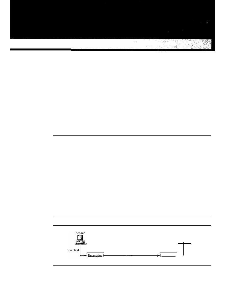
CHAPTER 30
Cryptography
Network security is mostly achieved through the use of cryptography, a science based
on abstract algebra. In this chapter, we briefly discuss the cryptography suitable for the
scope of this book. We have tried to limit our discussion of abstract algebra as much as
we could. Our goal is to give enough information about cryptography to make network
security understandable. The chapter opens the door for studying network security in
Chapter 31 and Internet security in Chapter 32.
30.1
INTRODUCTION
Let us introduce the issues involved in cryptography. First, we need to define some terms;
then we give some taxonomies.
Definitions
We define some terms here that are used in the rest of the chapter.
Cryptography
Cryptography,
a word with Greek origins, means "secret writing." However, we use the
term to refer to the science and
art
of transforming messages to make them secure and
immune to attacks. Figure 30.1 shows the components involved in cryptography.
Figure 30.1
Cryptography components
Receiver
Plaintext
Decryption
Ciphertext
931
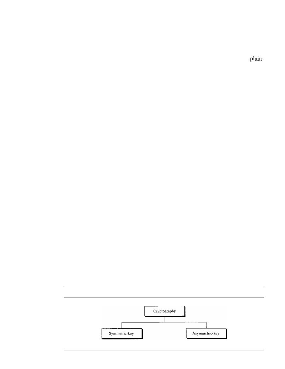
932
CHAPTER 30
CRYPTOGRAPHY
Plaintext and Ciphertext
The original message, before being transformed, is called
plaintext.
After the message
is transformed, it is called
ciphertext.
An
encryption algorithm
transforms the plain-
text into ciphertext; a
decryption algorithm
transforms the ciphertext back into
text. The sender uses an encryption algorithm, and the receiver uses a decryption
algorithm.
Cipher
We refer to encryption and decryption algorithms as
ciphers.
The term cipher is also
used to refer to different categories of algorithms in cryptography. This is not to say
that every sender-receiver pair needs their very own unique cipher for a secure commu-
nication. On the contrary, one cipher can serve millions of communicating pairs.
Key
A
key
is a number (or a set of numbers) that the cipher, as an algorithm, operates on. To
encrypt a message, we need an encryption algorithm, an encryption key, and the plaintext.
These create the ciphertext. To decrypt a message, we need a decryption algorithm, a
decryption key, and the ciphertext. These reveal the original plaintext.
Alice, Bob, and Eve
In cryptography, it is customary to use three characters in an information exchange
scenario; we use Alice, Bob, and Eve. Alice is the person who needs to send secure
data. Bob is the recipient of the data. Eve is the person who somehow disturbs the com-
munication between Alice and Bob by intercepting messages to uncover the data or by
sending her own disguised messages. These three names represent computers or pro-
cesses that actually send or receive data, or intercept or change data.
Two Categories
We can divide all the cryptography algorithms (ciphers) into two groups: symmetric-
key (also called
secret-key)
cryptography algorithms and asymmetric (also called
public-key)
cryptography algorithms. Figure 30.2 shows the taxonomy.
Figure 30.2
Categories of cryptography
Secret-key
Public-key
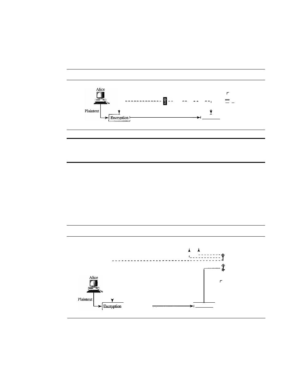
SECTION 30.1
INTRODUCTION
933
Symmetric·Key Cryptography
In symmetric-key cryptography, the same key is used by both parties. The sender uses
this key and an encryption algorithm to encrypt data; the receiver uses the same key and
the corresponding decryption algorithm to decrypt the data (see Figure 30.3).
Figure 30.3
Symmetric-key cryptography
Shared secret key
1 - -
--- -- --
1
I
1
I
Decryption
Ciphertext
Bob
-
Plaintext
In symmetric·key cryptography, the same key is used by the sender
(for encryption) and the receiver (for decryption).
The key
is
shared.
Asymmetric-Key Cryptography
In asymmetric or public-key cryptography, there are two keys: a private key and a public
key. The
private key
is kept by the receiver. The
public key
is announced to the public.
In Figure 30.4, imagine Alice wants to send a message to Bob. Alice uses the public key
to encrypt the message. When the message is received by Bob, the private key is used to
decrypt the message.
Figure 30.4
Asymmetric-key cryptography
To the public
I
1
Bob's public key
Bob's private key
1 - - - - -
Decryption
Ciphertext
Bob
Plaintext
In public-key encryption/decryption, the public key that is used for encryption is
different from the private key that is used for decryption. The public key is available to
the public;' the private key is available only to an individual.
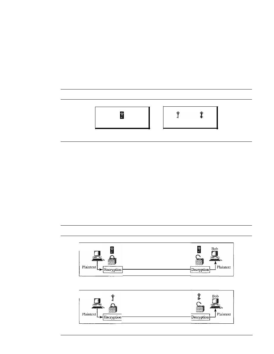
934
CHAPTER 30
CRYPTOGRAPHY
Three Types of Keys
The reader may have noticed that we are dealing with three types of keys in cryptography:
the secret key, the public key, and the private key. The first, the secret key, is the shared
key used in symmetric-key cryptography. The second and the third are the public
and private keys used in asymmetric-key cryptography. We will use three different icons
for these keys throughout the book to distinguish one from the others, as shown in
Figure 30.5.
Figure 30.5
Keys used in cryptography
Secret key
Symmetric-key cryptography
Public key
Private key
Asynunetric-key cryptography
Comparison
Let us compare symmetric-key and asymmetric-key cryptography. Encryption can be
thought of as electronic locking; decryption as electronic unlocking. The sender puts
the message in a box and locks the box by using a key; the receiver unlocks the box
with a key and takes out the message. The difference lies in the mechanism of the locking
and unlocking and the type of keys used.
In symmetric-key cryptography, the same key locks and unlocks the box. In
asymmetric-key cryptography, one key locks the box, but another key is needed to
unlock it. Figure 30.6 shows the difference.
Figure 30.6
Comparison between two categories of cryptography
Alice
Ciphertext
a. Symmetric-key cryptography
Alice
Ciphertext
b. Asymmetric-key cryptography
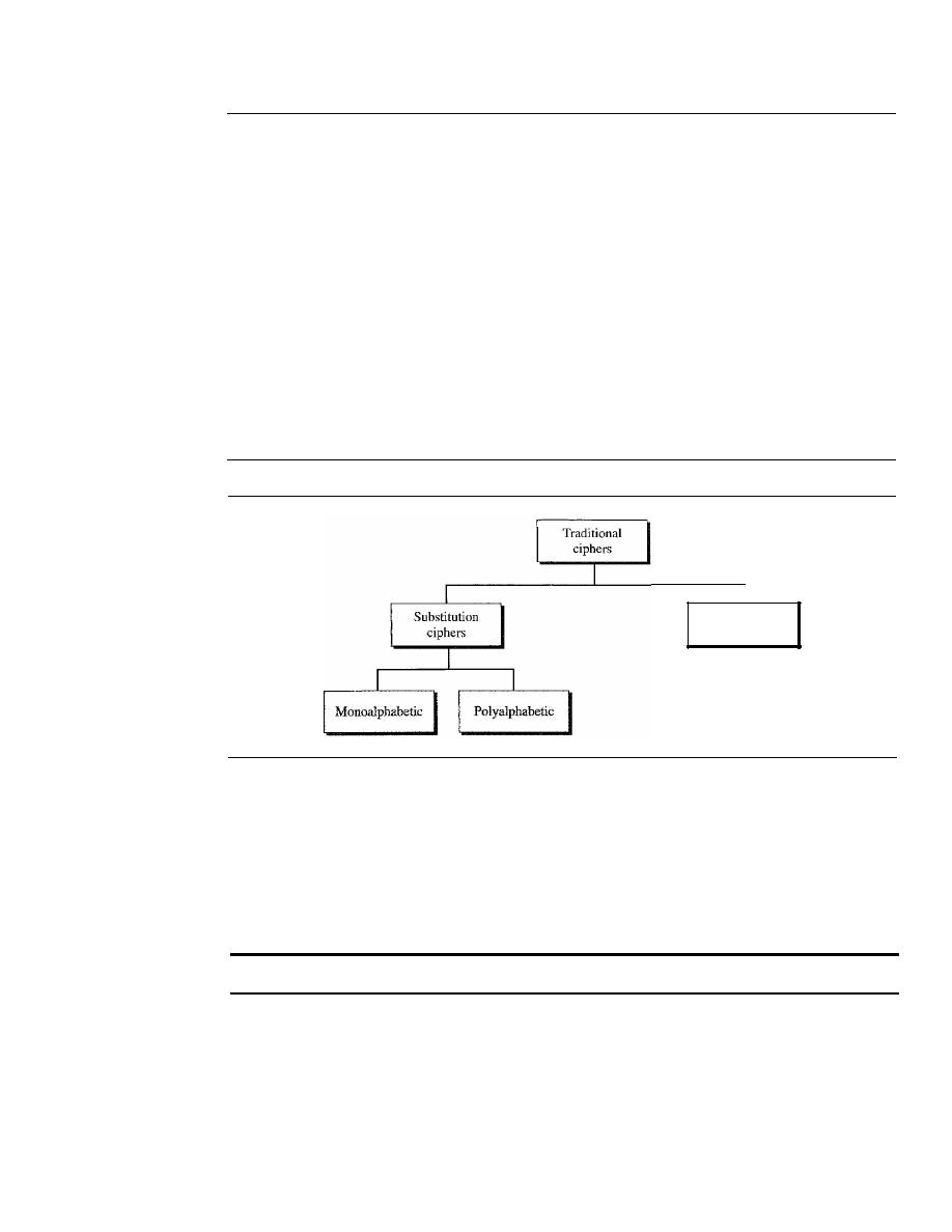
SECTION 30.2
SYMMETRIC-KEY CRYPTOGRAPHY
935
30.2
SYMMETRIC-KEY CRYPTOGRAPHY
Symmetric-key cryptography started thousands of years ago when people needed to
exchange secrets (for exanlple, in a war). We still mainly use symmetric-key cryptography
in our network security. However, today's ciphers are much more complex. Let us first
discuss traditional algorithms, which were character-oriented. Then we discuss the modem
ones, which are bit-oriented.
Traditional Ciphers
We briefly introduce some traditional ciphers, which are character-oriented. Although
these are now obsolete, the goal is to show how modern ciphers evolved from them. We
can divide traditional symmetric-key ciphers into two broad categories: substitution
ciphers and transposition ciphers, as shown in Figure 30.7.
Figure 30.7
Traditional ciphers
Transposition
ciphers
Substitution Cipher
A
substitution cipher
substitutes one symbol with another.
If
the symbols in the plain-
text are alphabetic characters, we replace one character with another. For example, we
can replace character A with D, and character T with Z.
If
the symbols are digits (0 to
9), we can replace 3 with 7, and 2 with 6. Substitution ciphers can be categorized as
either monoalphabetic or polyalphabetic ciphers.
A substitution cipher replaces one symbol with another.
In a
monoalphabetic cipher,
a character (or a symbol) in the plaintext is always
changed to the same character (or symbol) in the ciphertext regardless of its position in
the text. For example, if the algorithm says that character A in the plaintext is changed
to character D, every character A is changed to character D. In other words, the relation-
ship between characters in the plaintext and the ciphertext is a one-to-one relationship.
In a
polyalphabetic cipher,
each occurrence of a character can have a different
substitute. The relationship between a character in the plaintext to a character in the

936
CHAPTER 30
CRYPTOGRAPHY
ciphertext is a one-to-many relationship. For example, character A could be changed to
D in the beginning of the text, but it could be changed to N at the middle.
It
is obvious
that if the relationship between plaintext characters and ciphertext characters is one-to-
many, the key must tell us which of the many possible characters can be chosen for
encryption. To achieve this goal, we need to divide the text into groups of characters
and use a set of keys. For example, we can divide the text "THISISANEASYTASK"
into groups of 3 characters and then apply the encryption using a set of 3 keys. We then
repeat the procedure for the next 3 characters.
Example 30.1
The following shows a plaintext and its corresponding ciphertext. Is the cipher monoalphabetic?
Plaintext: HELLO
Ciphertext:
KHOOR
Solution
The cipher is probably monoalphabetic because both occurrences of L's are encrypted as O's.
Example 30.2
The following shows a plaintext and its corresponding ciphertext. Is the cipher monoalphabetic?
HELLO
Ciphertext: ABNZF
Solution
The cipher is not monoalphabetic because each occurrence of L is encrypted by a different char-
acter. The first L is encrypted as N; the second as Z.
Shift Cipher
The simplest monoalphabetic cipher is probably the shift cipher. We
assume that the plaintext and ciphertext consist of uppercase letters (A to Z) only. In
this cipher, the encryption algorithm is "shift
key
characters down," with
key
equal to
some number. The decryption algorithm is "shift
key
characters up." For example, if the
key is 5, the encryption algorithm is "shift 5 characters down" (toward the end of the
alphabet). The decryption algorithm is "shift 5 characters up" (toward the beginning of
the alphabet). Of course, if we reach the end or beginning of the alphabet, we wrap
around.
Julius Caesar used the shift cipher to communicate with his officers. For this reason,
the shift cipher is sometimes referred to as the Caesar cipher. Caesar used a key of 3
for his communications.
The shift cipher is sometimes referred to as the Caesar cipher.
Example 30.3
Use the shift cipher with key
=
15 to encrypt the message "HELLO."
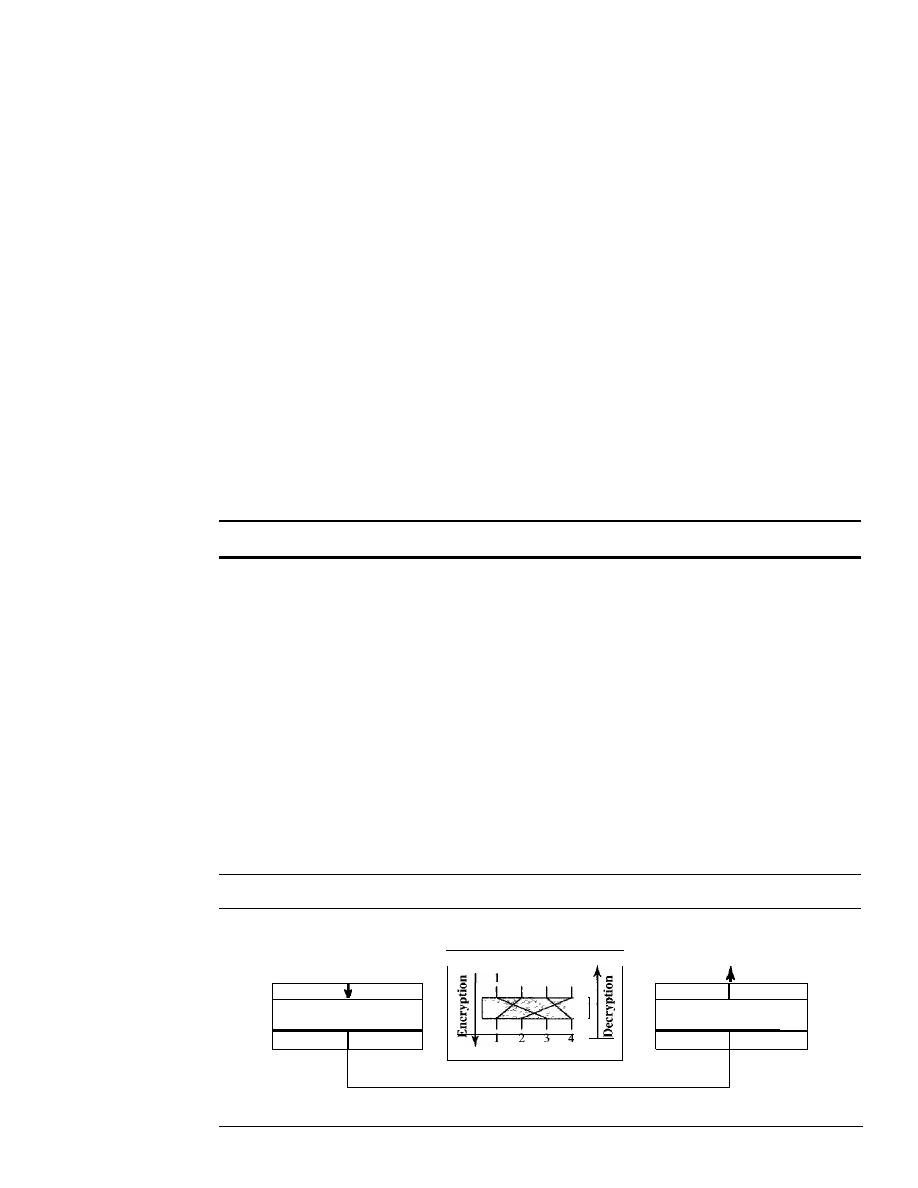
SECTION 30.2
SYMMETRIC-KEY CRYPTOGRAPHY
937
Solution
We encrypt one character at a time. Each character is shifted 15 characters down. Letter H is
encrypted to W. Letter E is encrypted to
T.
The first L is encrypted to A. The second L is also
encrypted to A. And 0 is encrypted to D. The cipher text is WTAAD.
Example 30.4
Use the shift cipher with key
=
15 to decrypt the message "WTAAD."
Solution
We decrypt one character at a time. Each character is shifted 15 characters up. Letter W is
decrypted to H. Letter T is decrypted to E. The first A is decrypted to
L.
The second A is
decrypted to
L.
And, finally, D is decrypted to O. The plaintext is HELLO.
Transposition Ciphers
In a
transposition cipher,
there is no substitution of characters; instead, their locations
change. A character in the first position of the plaintext may appear in the tenth position
of the ciphertext. A character in the eighth position may appear in the first position. In
other words, a transposition cipher reorders the symbols in a block of symbols.
A transposition cipher reorders (permutes) symbols in a block of symbols.
Key
In a transposition cipher, the key is a mapping between the position of the symbols
in the plaintext and cipher text. For example, the following shows the key using a block
of four characters:
Plaintext:
Ciphertext:
2 4 1 3
123 4
In encryption, we move the character at position 2 to position 1, the character at
position 4 to position 2, and so on. In decryption, we do the reverse. Note that, to be
more effective, the key should be long, which means encryption and decryption of long
blocks of data. Figure 30.8 shows encryption and decryption for our four-character
Figure 30.8
Transposition cipher
Plaintext
(block)
Key.
Plaintext
(block)
I
2 3
4
I
Reorder
I
I
Reorder
I
(downward direction)
(upward direction)
Encryption
Decryption
Ciphertext (block)
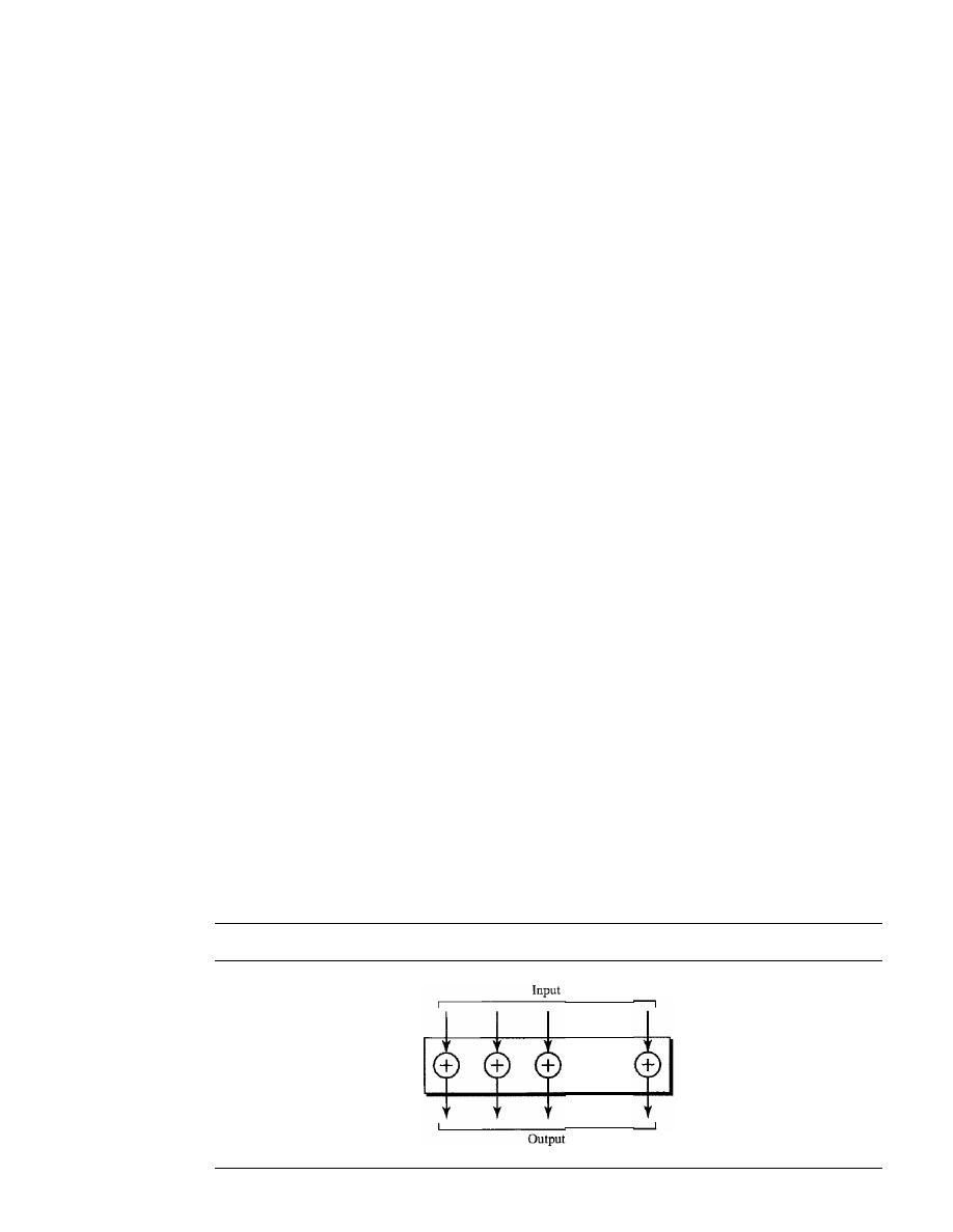
938
CHAPTER 30
CRYPTOGRAPHY
block using the above key. The figure shows that the encryption and decryption use the
same key. The encryption applies it from downward while decryption applies it upward.
Example 30.5
Encrypt the message "HELLO MY DEAR," using the above key.
Solution
We first remove the spaces in the message. We then divide the text into blocks of four characters.
We add a bogus character Z at the end of the third block. The result is HELL OMYD EARZ. We
create a three-block ciphertext ELHLMDOYAZER.
Example 30.6
Using Example 30.5, decrypt the message "ELHLMDOYAZER".
Solution
The result is HELL OMYD EARZ. After removing the bogus character and combining the char-
acters, we get the original message "HELLO MY DEAR."
Simple Modern Ciphers
The traditional ciphers we have studied so far are character-oriented. With the advent of
the computer, ciphers need to be bit-oriented. This is so because the information to be
encrypted is not just text; it can also consist of numbers, graphics, audio, and video data.
It
is convenient to convert these types of data into a stream of bits, encrypt the stream,
and then send the encrypted stream. In addition, when text is treated at the bit level, each
character is replaced by 8 (or 16) bits, which means the number of symbols becomes 8
(or 16). Mingling and mangling bits provides more security than mingling and mangling
characters. Modem ciphers use a different strategy than the traditional ones. A modern
symmetric cipher is a combination of simple ciphers. In other words, a modern cipher
uses several simple ciphers to achieve its goal. We first discuss these simple ciphers.
XOR
Cipher
Modern ciphers today are normally made of a set of simple ciphers, which are simple
predefined functions in mathematics or computer science. The first one discussed here
is called the XOR cipher because it uses the exclusive-or operation as defined in computer
science. Figure 30.9 shows an XOR cipher.
Figure 30.9
XOR cipher
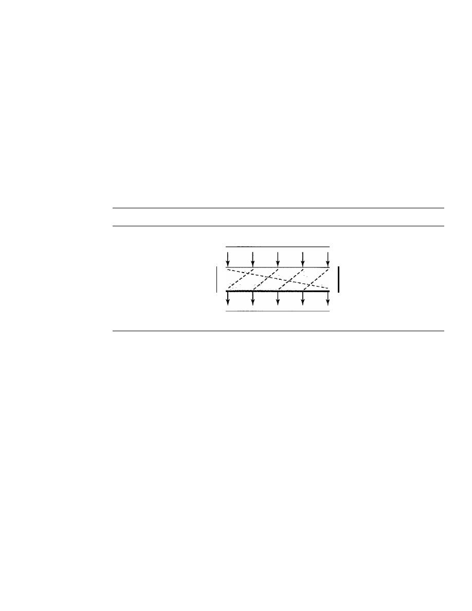
SECTION 30.2
SYMMETRIC-KEY CRYPTOGRAPHY
939
An XOR operation needs two data inputs plaintext, as the first and a key as the sec-
ond. In other words, one of the inputs is the block to be the encrypted, the other input is
a key; the result is the encrypted block. Note that in an XOR cipher, the size of the key,
the plaintext, and the ciphertext are all the same. XOR ciphers have a very interesting
property: the encryption and decryption are the same.
Rotation Cipher
Another common cipher is the
rotation cipher,
in which the input bits are rotated to
the left or right. The rotation cipher can be keyed or keyless. In keyed rotation, the value of
the key defines the number of rotations; in keyless rotation the number of rotations is fixed.
Figure 30.10 shows an example of a rotation cipher. Note that the rotation cipher can be
considered a special case of the transpositional cipher using bits instead of characters.
Figure 30.10
Rotation cipher
Input
Output
The rotation cipher has an interesting property.
If
the length of the original stream
is
N,
after
N
rotations, we get the original input stream. This means that it is useless to
apply more than
N -
1 rotations. In other words, the number of rotations must be between
1 and
N-1.
The decryption algorithm for the rotation cipher uses the same key and the opposite
rotation direction. If we use a right rotation in the encryption, we use a left rotation in
decryption and vice versa.
Substitution Cipher: S-box
An S-box (substitution box) parallels the traditional substitution cipher for characters.
The input to an S-box is a stream of bits with length
N;
the result is another stream of
bits with length
M.
And Nand
M
are not necessarily the same. Figure 30.11 shows an
S-box.
The S-box is normally keyless and is used as an intermediate stage of encryption
or decryption. The function that matches the input to the output may be defined mathe-
matically or by a table.
Transposition Cipher: P-box
A P-box (permutation box) for bits parallels the traditional transposition cipher for char-
acters.
It
performs a transposition at the bit level; it transposes bits.
It
can be implemented
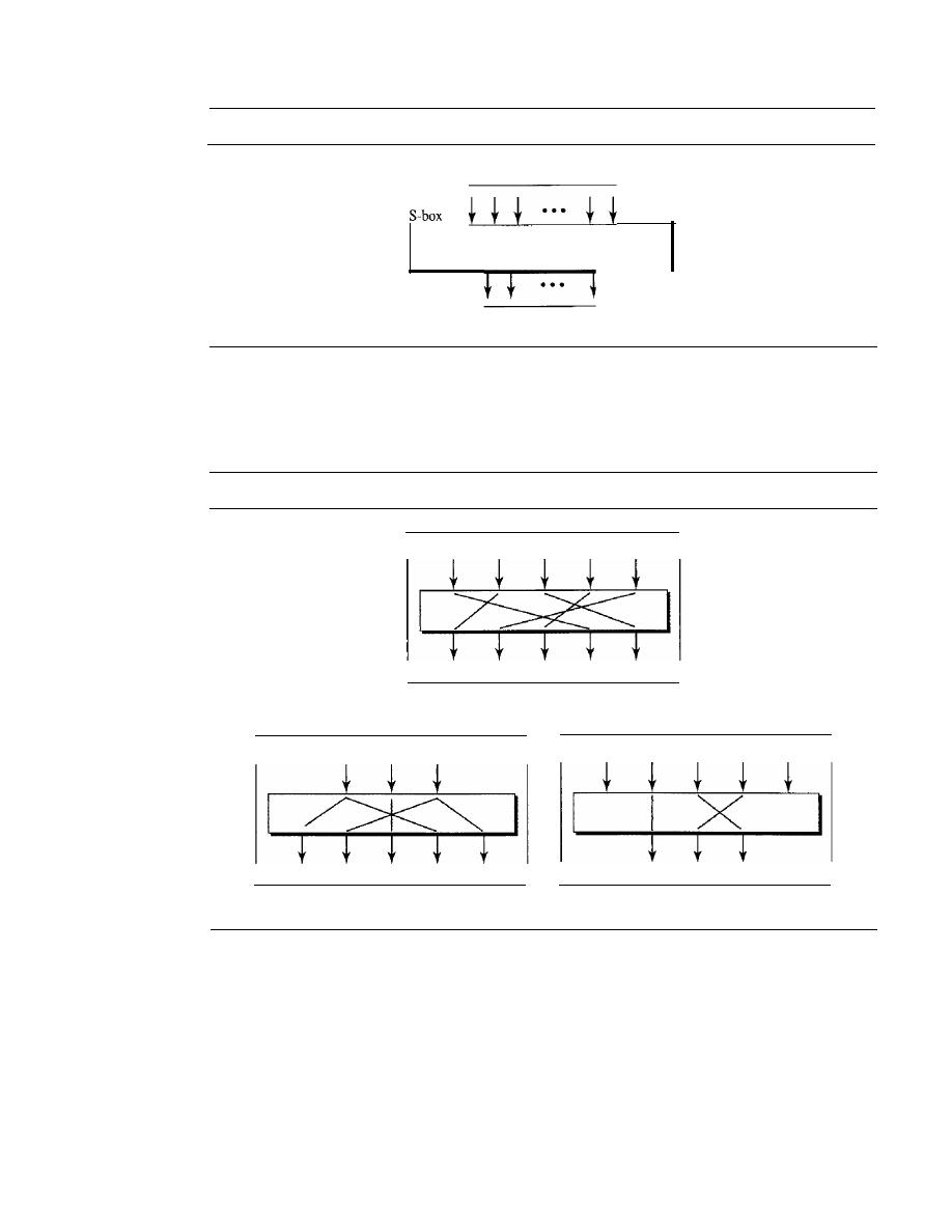
940
CHAPTER 30
CRYPTOGRAPHY
Figure 30.11
S-box
N
input bits
A function that matches
N
inputs
toM outputs
M
output bits
in software or hardware, but hardware is faster. P-boxes, like S-boxes, are nonnally key-
less. We can have three types of pennutations in P-boxes: the straight permutation,
expansion permutation, and compression permutation as shown in Figure 30.12.
Figure 30.12
P-boxes: straight, expansion, and compression
2
3
4
5
2
2
3
a. Straight
3
4
5
2
3
4
5
2
3
2
4
3
5
b. Expansion
c. Compression
A straight permutation cipher or a straight P-box has the same number of inputs as
outputs. In other words, if the number of inputs is
N,
the number of outputs is also
N.
In
an expansion pennutation cipher, the number of output ports is greater than the number
of input ports. In a compression pennutation cipher, the number of output ports is less
than the number of input ports.
Modern Round Ciphers
The ciphers of today are called round ciphers because they involve multiple rounds,
where each round is a complex cipher made up of the simple ciphers that we previously
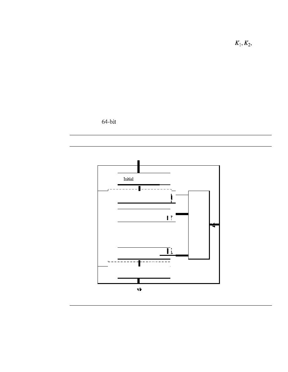
SECTION 30.2
SYMMETRIC-KEY CRYPTOGRAPHY
941
described. The key used in each round is a subset or variation of the general key called the
round key.
If
the cipher has
N
rounds, a key generator produces
N
keys,
..., K
N ,
where K
1
is used in round 1,
K
2
in round 2, and so on.
In this section, we introduce two modem symmetric-key ciphers: DES and AES.
These ciphers are referred to as
block ciphers
because they divide the plaintext into
blocks and use the same key to encrypt and decrypt the blocks. DES has been the de
facto standard until recently. AES is the formal standard now.
Data Encryption Standard (DES)
One example of a complex block cipher is the
Data Encryption Standard (DES).
DES
was designed by IBM and adopted by the U.S. government as the standard encryption
method for nonmilitary and nonclassified use. The algorithm encrypts a 64-bit plaintext
block using a
key, as shown in Figure 30.13.
Figure 30.13
DES
64-bit plaintext
DES
I
permutation
I
I
I
I
K
j
Round 1
I
•
I
I
I
I
I
K
2
Round 2
Round
key
•
•
generator
•
•
•
·
K
l6
I
Round 16
I
I
Final permutation
I
64-bit key
64-bit ciphertext
DES has two transposition blocks (P-boxes) and 16 complex round ciphers (they are
repeated). Although the 16 iteration round ciphers are conceptually the same, each uses
a different key derived from the original key.
The initial and final permutations are keyless straight permutations that are the
inverse of each other. The permutation takes a 64-bit input and permutes them according
to predefined values.
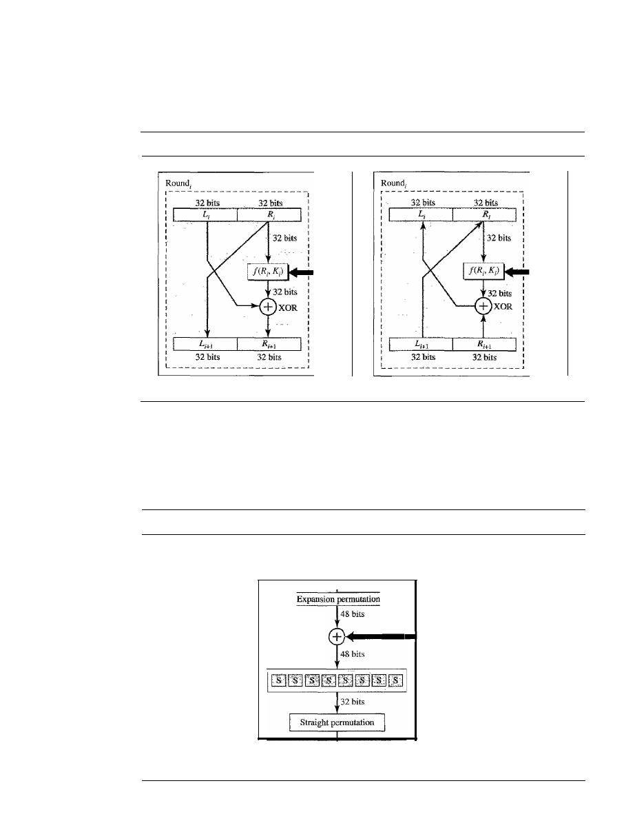
942
CHAPTER 30
CRYPTOGRAPHY
Each round of DES is a complex round cipher, as shown in Figure 30.14. Note that
the structure of the encryption round ciphers is different from that of the decryption one.
Figure 30.14
One round in DES ciphers
K
j
(48 bits)
a. Encryption round
b. Decryption round
K;
(48 bits)
DES Function
The heart of DES is the DES function. The DES function applies a
48-bit key to the rightmost 32 bits R
i
to produce a 32-bit output. This function is made
up of four operations: an XOR, an expansion permutation, a group of S-boxes, and a
straight permutation, as shown in Figure 30.15.
Figure 30.15
DES function
R;
(32
bits)
Function
S-boxes
XOR
- K;
(48 bits)
32
bits
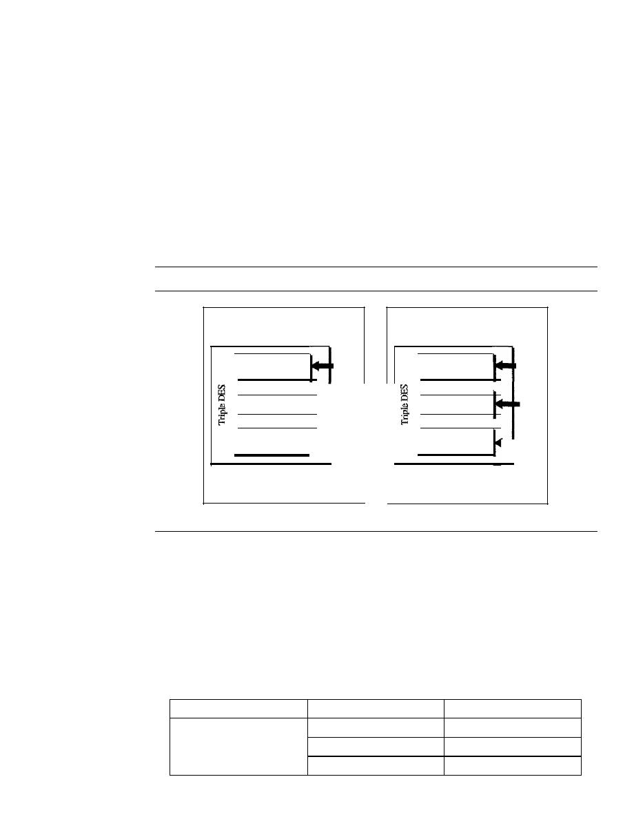
SECTION 30.2
SYMMETRIC-KEY CRYPTOGRAPHY
943
Triple DES
Critics of DES contend that the key is too short. To lengthen the key,
Triple DES
or 3DES
has been proposed and implemented. This uses three DES blocks, as shown in Figure 30.16.
Note that the encrypting block uses an encryption-decryption-encryption combination of
DESs, while the decryption block uses a decryption-encryption-decryption combination.
Two different versions of 3DES are in use: 3DES with two keys and 3DES with three keys.
To make the key size 112 bits and at the same time protect DES from attacks such as the
man-in-the-middle attack, 3DES with two keys was designed.
In
this version, the first and
the third keys are the same (KeYl
=
KeY3)' This has the advantage in that a text encrypted by
a single DES block can be decrypted by the new 3DES. We just set
all
keys equal to KeYl'
Many algorithms use a 3DES cipher with three keys. This increases the size of the key
to 168 bits.
Figure 30.16
Triple DES
64-bit plaintext
64-bit plaintext
Encrypt DES
KeYl
Decrypt DES
KeYl
Decrypt DES
KeY2
Encrypt DES
KeY2
Encrypt DES
KeY3
Decrypt DES
KeY3
64-bit ciphertext
64-bit ciphertext
a. Encryption Triple DES
b. Decryption Triple DES
Advanced Encryption Standard (AES)
The
Advanced Encryption Standard (AES)
was designed because DES's key was too
small. Although Triple DES ODES) increased the key size, the process was too slow.
The
National Institute of Standards and Technology (NIST)
chose the
Rijndael
algorithm,
named after its two Belgian inventors, Vincent Rijmen and Joan Daemen,
as the basis of AES. AES is a very complex round cipher. AES is designed with three
key sizes: 128, 192, or 256 bits. Table 30.1 shows the relationship between the data block,
number of rounds, and key size.
Table 30.1
AES configuration
Size ofData Block
Number ofRounds
Key
Size
10
128 bits
128 bits
12
192 bits
14
256 bits
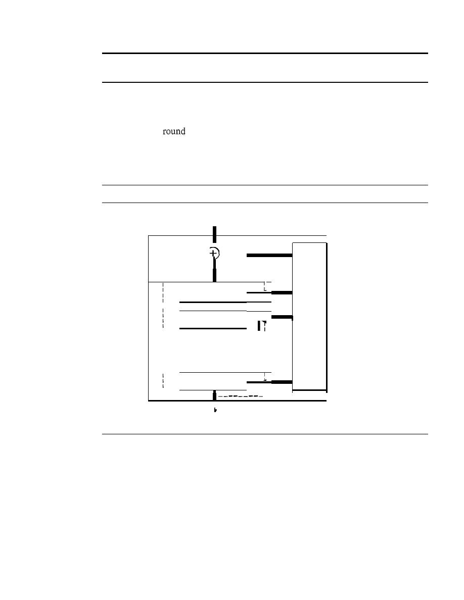
944
CHAPTER 30
CRYPTOGRAPHY
AES has three different configurations with respect
to the number of rounds and key size.
In this text, we discuss just the lO-round, 12S-bit key configuration. The structure and
operation of the other configurations are similar. The difference lies in the key generation.
The general structure is shown in Figure 30.17. There is an initial XOR operation
followed by 10
ciphers. The last round is slightly different from the preceding
rounds; it is missing one operation.
Although the 10 iteration blocks are almost identical, each uses a different key
derived from the original key.
Figure 30.17
AES
12S-bit plaintext
AES
K
o
r - - - - - - - - -
-----------,
I
I
K
1
Ronnd 1
I
I
I
•
I
I
I
Round
I
I
K
2
key
Round 2
generator
I
I
I
I
I
I
·
I
I
·
I
·
·
I
·
I
·
I
I
I
I
I
I
I
Round 10
I
K
IO
(slightly different)
I
I
I
'------------
1
,
12S-bit key
l2S-bit ciphertext
Structure of Each Round
Each round of AES, except for the last, is a cipher with four
operations that are invertible. The last round has only three operations. Figure 30.18 is
a flowchart that shows the operations in each round. Each of the four operations used in
each round uses a complex cipher; this topic is beyond the scope of this book.
Other Ciphers
During the last two decades, a few other symmetric block ciphers have been designed and
used. Most of these ciphers have similar characteristics to the two ciphers we discussed in
this chapter (DES and AES). The difference is usually in the size of the block or key, the
number of rounds, and the functions used. The principles are the same. In order not to
burden the user with the details of these ciphers, we give a brief description of each.
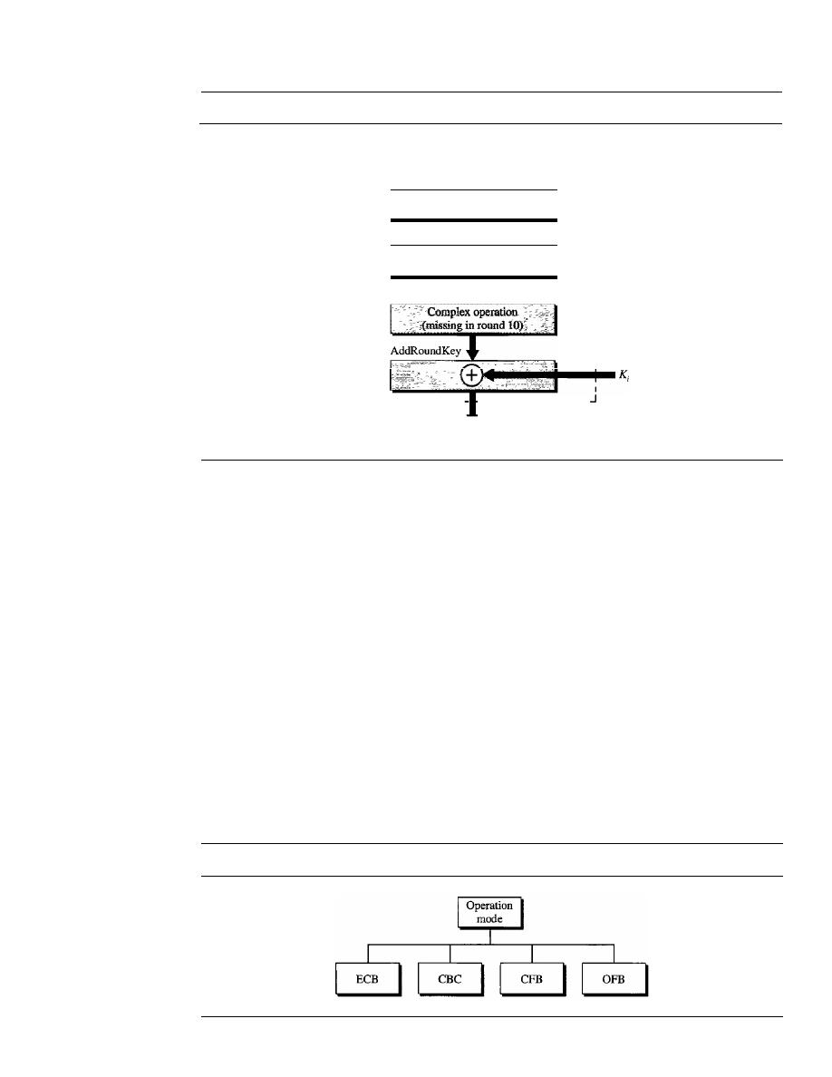
SECTION 30.2
SYMMETRIC-KEY CRYPTOGRAPHY
945
Figure 30.18
Structure of each round
Round
i
SubByte
128-bit data
Byte substitution
ShiftRow
Byte permutation
MixCo1umn
1_ _ _ _ _ _ _ _ _ _ _ _ _
_
128-bit data
IDEA
The International Data Encryption Algorithm (IDEA) was developed by Xuejia
Lai and James Massey. The block size is 64 and the key size is 128.
It
can be imple-
mented in both hardware and software.
Blowfish
Blowfish was developed by Bruce Schneier. The block size is 64 and the
key size between 32 and 448.
CAST-128
CAST-128 was developed by Carlisle Adams and Stafford Tavares.
It
is a
Feistel cipher with 16 rounds and a block size of 64 bits; the key size is 128 bits.
ReS
RCS was designed by Ron Rivest.
It
is a family of ciphers with different block
sizes, key sizes, and numbers of rounds.
Mode of Operation
A mode of operation is a technique that employs the modern block ciphers such as DES
andAES that we discussed earlier (see Figure 30.19).
Figure 30.19
Modes of operation for block ciphers
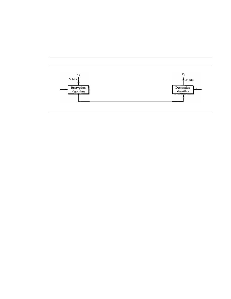
946
CHAPTER 30
CRYPTOGRAPHY
Electronic Code Book
The electronic code book (ECB) mode is a purely block cipher technique. The plain-
text is divided into blocks of
N
bits. The ciphertext is made of blocks of
N
bits. The
value of
N
depends on the type of cipher used. Figure 30.20 shows the method.
Figure 30.20
ECB mode
K
Pi: Plaintext block
i
C
i:
Ciphertext block
i
Nbits
K
We mention four characteristics of this mode:
1.
Because the key and the encryption/decryption algorithm are the same, equal blocks
in the plaintext become equal blocks in the ciphertext. For example, if plaintext
blocks 1, 5, and 9 are the same, ciphertext blocks I, 5, and 9 are also the same.
This can be a security problem; the adversary can guess that the plaintext blocks
are the same if the corresponding ciphertext blocks are the same.
2.
If
we reorder the plaintext block, the ciphertext is also reordered.
3. Blocks are independent of each other. Each block is encrypted or decrypted inde-
pendently. A problem in encryption or decryption of a block does not affect other
blocks.
4. An error in one block is not propagated to other blocks.
If
one or more bits are cor-
rupted during transmission, it only affects the bits in the corresponding plaintext
after decryption. Other plaintext blocks are not affected. This is a real advantage if
the channel is not noise-free.
Cipher Block Chaining
The cipher block chaining (CBC) mode tries to alleviate some of the problems in ECB
by including the previous cipher block in the preparation of the current block.
If
the cur-
rent block is
i,
the previous ciphertext block C
i- 1
is included in the encryption of block
i.
In other words, when a block is completely enciphered, the block is sent, but a copy of it
is kept in a register (a place where data can be held) to be used in the encryption of the
next block. The reader may wonder about the initial block. There is no ciphertext block
before the first block. In this case, a phony block called the initiation vector (IV) is
used. Both the sender and receiver agree upon a specific predetermined IV. In other
words, the IV is used instead of the nonexistent CO, Figure 30.21 shows the CBC mode.
The reader may wonder about the decryption. Does the configuration shown in the
figure guarantee the correct decryption?
It
can be proven that it does, but we leave the
proof to a textbook in network security.
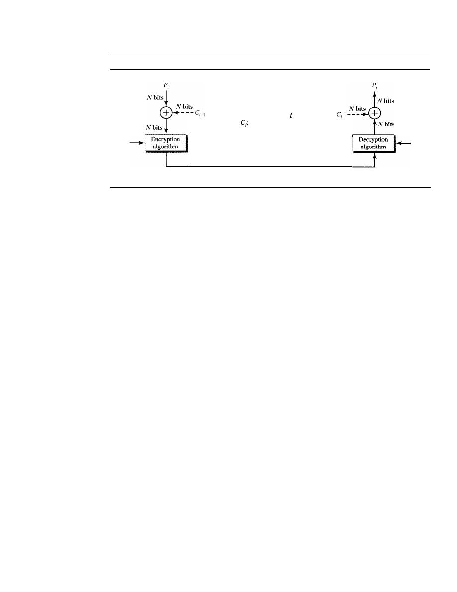
SECTION 30.2
SYMMETRIC-KEY CRYPTOGRAPHY
947
Figure 30.21
CBC mode
K
Initiated
with IV
F,:
Plaintext block
Ciphertext block
i
IV: Initialization vector
N
bits
Initiated
with IV
K
The following are some characteristics of CBC.
1.
Even though the key and the encryption/decryption algorithm are the same, equal
blocks in the plaintext do not become equal blocks in the ciphertext. For example,
if plaintext blocks
1,
5, and 9 are the same, ciphertext blocks I, 5, and 9 will not be
the same. An adversary will not be able to guess from the ciphertext that two blocks
are the same.
2. Blocks are dependent on each other. Each block is encrypted or decrypted based on
a previous block. A problem in encryption or decryption of a block affects other
blocks.
3.
The error in one block is propagated to the other blocks.
If
one or more bits are
corrupted during the transmission, it affects the bits in the next blocks of the plain-
text after decryption.
Cipher Feedback
The cipher feedback (CFB) mode was created for those situations in which we need
to send or receive
r
bits of data, where
r
is a number different from the underlying
block size of the encryption cipher used. The value of
r
can be
1,
4, 8, or any number of
bits. Since all block ciphers work on a block of data at a time, the problem is how to
encrypt just
r
bits. The solution is to let the cipher encrypt a block of bits and use only
the first
r
bits as a new key (stream key) to encrypt the
r
bits of user data. Figure 30.22
shows the configuration.
The following are some characteristics of the CFB mode:
1.
If
we change the IV from one encryption to another using the same plaintext, the
ciphertext is different.
2. The ciphertext C
i
depends on both Pi and the preceding ciphertext block.
3. Errors in one or more bits of the ciphertext block affect the next ciphertext blocks.
Output Feedback
The
output
feedback (OFB) mode is very similar to the CFB mode with one difference.
Each bit in the ciphertext is independent of the previous bit or bits. This avoids error
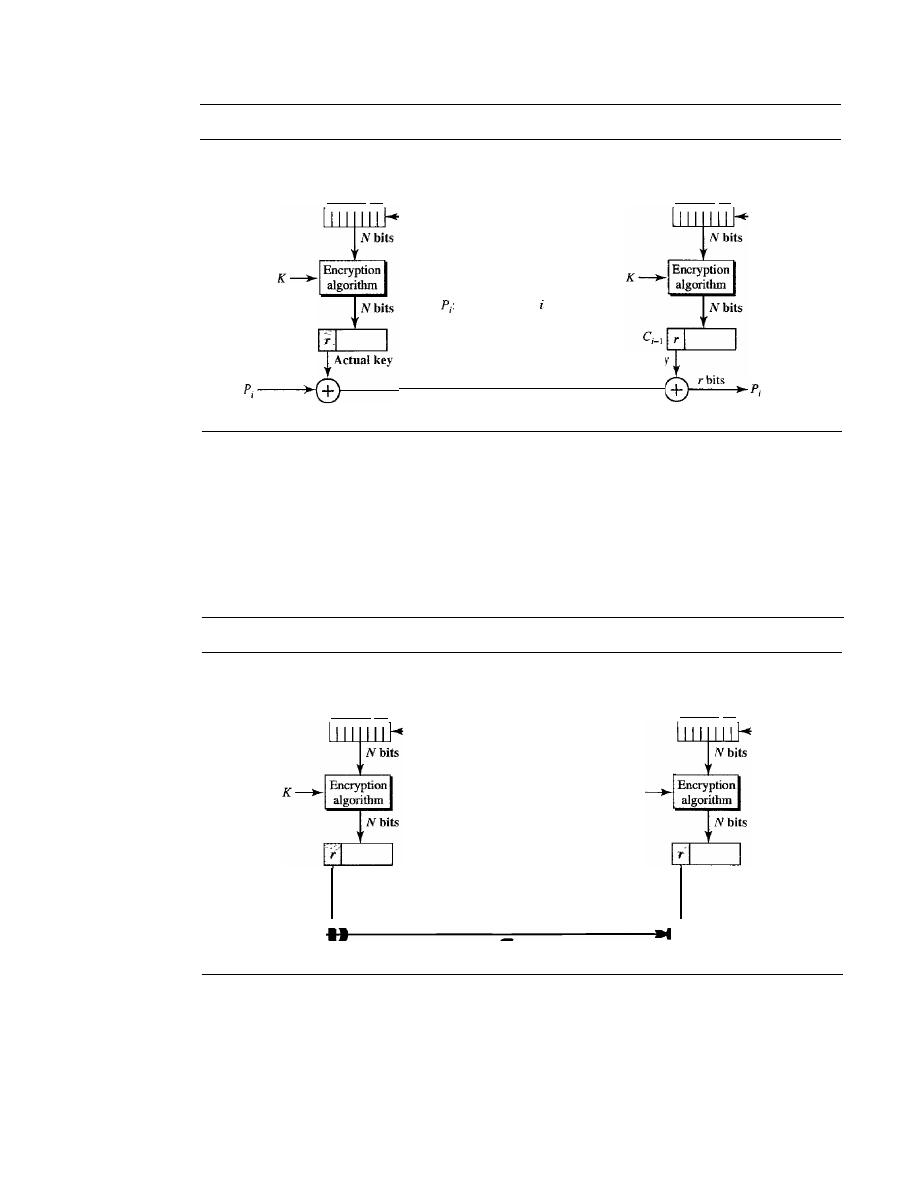
948
CHAPTER 30
CRYPTOGRAPHY
Figure 30.22
CFB mode
N-bit
shift register
initially IV
rbits
r
bits
- - - C
i_
1
Plaintext block
C
i
:
Ciphertext block
i
IV: Initialization vector
r
bits
Actual key
N-bit
shift register
initially IV
r
bits
---C
i-
1
propagation.
If
an error occurs in transmission, it does not affect the future bits. Note
that, as in CFB, both the sender and the receiver use the encryption algorithm. Note
also that in OFB, block ciphers such as DES or AES can only be used to create the key
stream. The feedback for creating the next bit stream comes from the previous bits of
the key stream instead of the ciphertext. The ciphertext does not take part in creating
the key stream. Figure 30.23 shows the OFB mode.
Figure 30.23
OFB mode
N-bit
shift register
initially IV
Actual key
r
bits
Pi:
Plaintext block
i
C
j :
Ciphertext block
i
IV: Initialization vector
K
N-bit
shift register
initially IV
Actual key
r
bits
r
bits
+
r
bits
Pi
Pi
C
i
The following are some of the characteristics of the OFB mode.
1.
If
we change the IV from one encryption to another using the same plaintext, the
ciphertext will be different.
2. The ciphertext C
i
depends on the plaintext
Pi'
3. Errors in one or more bits of the ciphertext do not affect future ciphertext blocks.
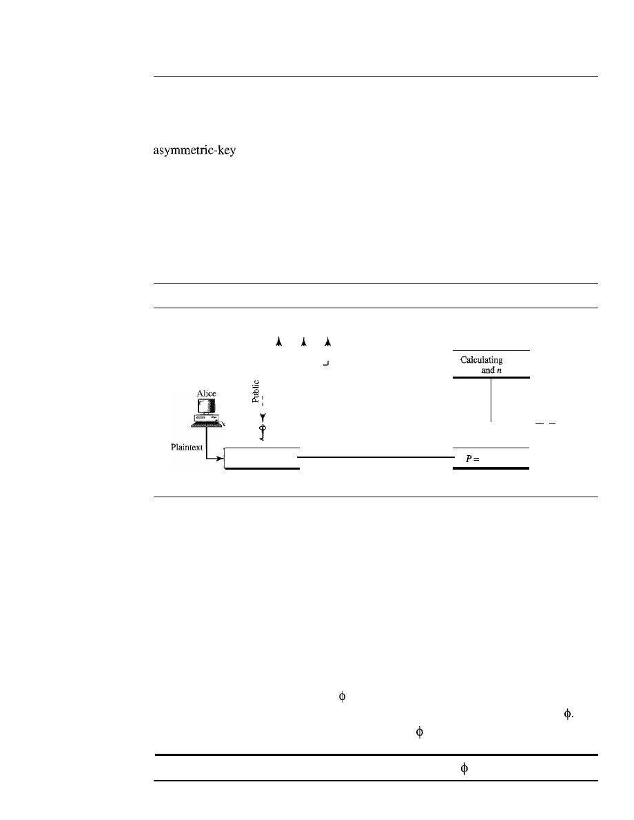
SECTION 30.3
ASYMMETRIC-KEY CRYPTOGRAPHY
949
30.3
ASYMMETRIC-KEY CRYPTOGRAPHY
In the previous sections, we discussed symmetric-key cryptography. In this section we
introduce asymmetric-key (public key cryptography). As we mentioned before, an
(or public-key) cipher uses two keys: one private and one public. We
discuss two algorithms: RSA and Diffie-Hellman.
RSA
The most common public key algorithm is RSA, named for its inventors Rivest, Shamir,
and Adleman (RSA).
It
uses two numbers, e and d, as the public and private keys, as
shown in Figure 30.24.
Figure 30.24
RSA
To public
,
,
I
I
,
I
, __ L
L __
_
I
:
,
e
,
C=pemodn
Encryption
Ciphertext
e,
d,
Cemodn
Decryption
Bob
- -
Plaintext
The two keys,
e
and
d,
have a special relationship to each other, a discussion of this
relationship is beyond the scope of this book. We just show how to calculate the keys
without proof.
Selecting Keys
Bob use the following steps to select the private and public keys:
1.
Bob chooses two very large prime numbers
p
and
q.
Remember that a prime num-
ber is one that can be divided evenly only by 1 and itself.
2. Bob multiplies the above two primes to find
n,
the modulus for encryption and
decryption. In other words,
n :::
p
X
q.
3. Bob calculates another number
:::
(p
-1)
X
(q -
1).
4. Bob chooses a random integer
e.
He then calculates
d
so that
d
x
e:::
1 mod
5. Bob announces e and n to the public; he keeps
and
d
secret.
In RSA,
e and n are announced to the public;
d
and
are kept secret.
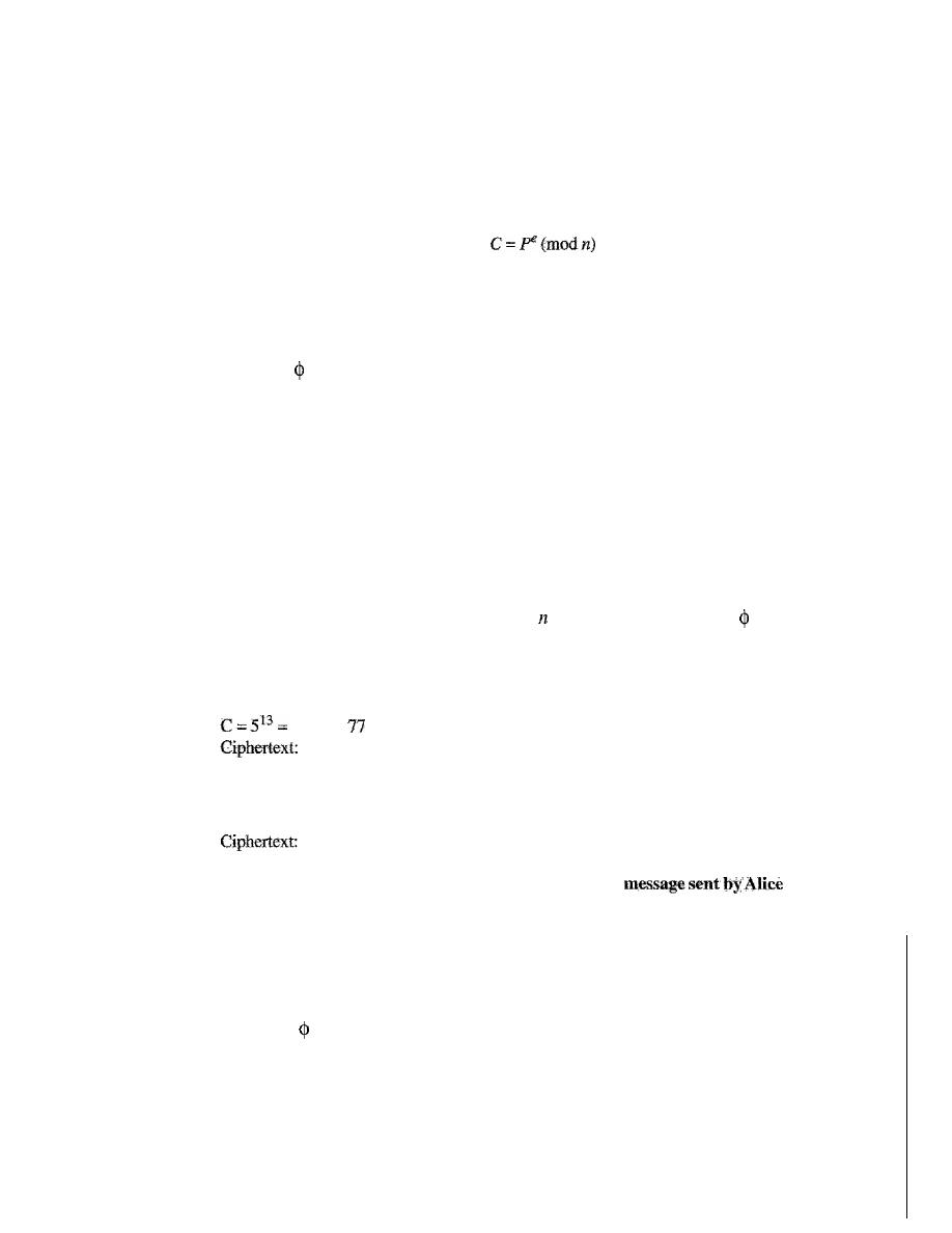
950
CHAPTER 30
CRYPTOGRAPHY
Encryption
Anyone who needs to send a message to Bob can use nand
e.
For example, if Alice
needs to send a message to Bob, she can change the message, usually a short one, to an
integer. This is the plaintext. She then calculates the ciphertext, using e and n.
Alice sends C, the ciphertext, to Bob.
Decryption
Bob keeps
and
d
private. When he receives the ciphertext, he uses his private key
d
to
decrypt the message:
P=
Cd(modn)
Restriction
For RSA to work, the value of
P
must be less than the value of n.
If
P
is a large number,
the plaintext needs to be divided into blocks to make P less than
n.
Example 30.7
Bob chooses 7 and 11 as p and q and calculates
= 7 . 11 = 77. The value of
= (7 - 1) (11 - 1)
or 60. Now he chooses two keys, e and
d.
If
he chooses e to be 13, then dis 37. Now imagine
Alice sends the plaintext 5 to Bob. She uses the public key 13 to encrypt 5.
Plaintext:
5
26 mod
26
Bob receives the ciphertext 26 and uses the private key 37 to decipher the ciphertext:
26
P
=
26
37
=
5
mod
77
Plaintext: 5
Intended
The plaintext 5 sent by Alice is received as plaintext 5 by Bob.
Example 30.8
Jennifer creates a pair of keys for herself. She chooses p
=
397 and q
=
401. She calculates n
=
159,197 and
=
396 . 400
=
158,400. She then chooses e
=
343 and
d
=
12,007. Show how Ted
can send a message to Jennifer if he knows
e
and
n.
Solution
Suppose Ted wants to send the message "NO" to Jennifer. He changes each character to a number
(from 00 to 25) with each character coded as two digits. He then concatenates the two coded
characters and gets a four-digit number. The plaintext is 1314. Ted then uses
e
and
n
to encrypt
the message. The ciphertext is 1314
343
= 33,677 mod 159,197. Jennifer receives the message
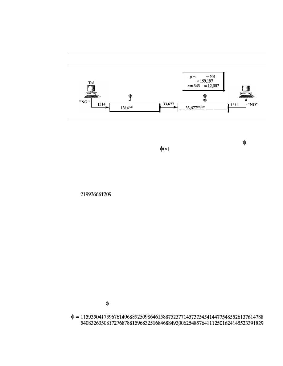
SECTION 30.3
ASYMMETRIC-KEY CRYPTOGRAPHY
951
33,677 and uses the decryption key
d
to decipher it as 33,677
12
,007
=
1314 mod 159,197. Jennifer
then decodes 1314 as the message "NO". Figure 30.25 shows the process.
Figure 30.25
Example 30.8
Jennifer
d= 12,007
391 q
n
d
P
=
mod 159,197
e
=
343
C
=
mod 159,197
Example 30.9
Let us give a realistic example. We choose a
512-bitp
and
q.
We calculate nand
We then
choose
e
and test for relative primeness with
We calculate
d.
Finally, we show the results of
encryption and decryption. We have written a program written in Java to do so; this type of calcula-
tion cannot be done by a calculator.
We randomly chose an integer of 512 bits. The integer
p
is a 159-digit number.
p=96130345313583504574191581280615427909309845594996215822583150879647940
45505647063849125716018034750312098666606492420191808780667421096063354
The integer
q
is a 160-digitnumber.
q=
12060191957231446918276794204450896001555925054637033936061798321731482
14848376465921538945320917522527322683010712069560460251388714552496900
0359660045617
We calculate
n.
It
has 309 digits.
n=11593504I73967614968892509864615887523771457375454144775485526137614788
54083263508172768788159683251684688493006254857641112501624145523391829
27162507656772727460097082714127730434960500556347274566628060099924037
10299142447229221577279853172703383938133469268413732762200096667667183
1831088373420823444370953
We calculate
It
has 309 digits:
27162507656751054233608492916752034482627988117554787657013923444405716
98958172819609822636107546721186461217135910735864061400888517026537727
1264467341066243857664128
952
CHAPTER 30
CRYPTOGRAPHY
We choose
e
=
35,535.
We then find
d.
=
d=58oo8302860037763936093661289677917594669062089650962180422866111380593852
82235873170628691003002171085904433840217072986908760061153062025249598844
48047568240966247081485817130463240644077704833134010850947385295645071936
77406119732655742423721761767462077637164207600337085333288532144708859551
36670294831
Alice wants to send the message "THIS IS A TEST" which can be changed to a numeric
value by using the
00-26
encoding scheme
(26
is the
space
character).
P
=
1907081826081826002619041819
The ciphertext calculated by Alice is C
=
p
e
,
which is
c
60613199328566617843418359114151197411252005682979794571736036101278:21'
8847892741566090480023507190715277185914975188465888632101148354103361
6578984679683867637337657774656250792805211481418440481418443081277305",
9004692874248559166462108656
Bob can recover the plaintext from the ciphertext by using
P
=
Cd,
which is
P
1907081826081826002619041819
The recovered plaintext is THIS IS A TEST after decoding.
Applications
Although RSA can be used to encrypt and decrypt actual messages, it is very slow if the
message is long. RSA, therefore, is useful for short messages such as a small message
digest (see Chapter 31) or a symmetric key to be used for a symmetric-key cryptosystem.
In particular, we will see that RSA is used in digital signatures and other cryptosystems
that often need to encrypt a small message without having access to a symmetric key.
RSA is also used for authentication as we will see later.
Diffie-Hellman
RSA is a public-key cryptosystem that is often used to encrypt and decrypt symmetric
keys. Diffie-Hellman, on the other hand, was originally designed for key exchange. In the
Diffie-Hellman
cryptosystem,
two parties create a symmetric
session key
to exchange
data without having to remember or store the key for future use. They do not have to meet
to agree on the key; it can be done through the Internet. Let us see how the protocol works
when Alice and Bob need a symmetric key to communicate. Before establishing a sym-
metric key, the two parties need to choose two numbers
p
and
g.
The first number,
p,
is a
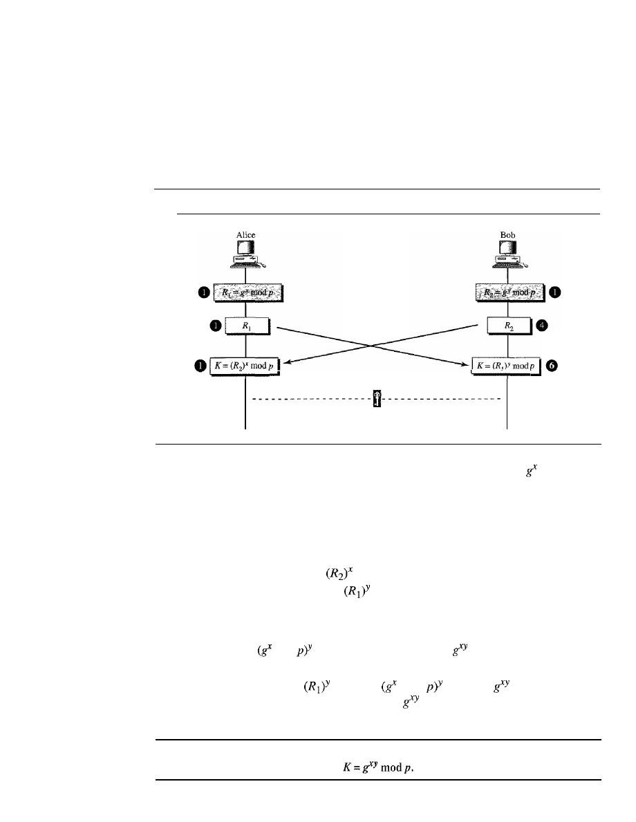
SECTION 30.3
ASYMMETRIC-KEY CRYPTOGRAPHY
953
large prime number on the order of 300 decimal digits (1024 bits). The second number is
a random number. These two numbers need not be confidential. They can be sent through
the Internet; they can be public.
Procedure
Figure 30.26 shows the procedure. The steps are as follows:
Figure 30.26
Diffie-Hellman method
The values of
p
and g are public.
Shared secret key
K=gXY
modp
o
Step
1:
Alice chooses a large random number
x and calculates R
1
=
mod
p.
o
Step 2: Bob chooses another large random number
y
and calculates R2
=
gY
mod p.
o
Step 3: Alice sends R
1
to Bob. Note that Alice does not send the value of
x;
she
sends only R
1-
o
Step 4: Bob sends
R
2
to Alice. Again, note that Bob does not send the value of y,
he sends only R
2 .
o
Step 5: Alice calculates
K
=
mod
p.
o
Step 6: Bob also calculates
K
=
mod
p.
The symmetric key for the session is K.
mod
mod
p
=
(gY
mod
p)X
mod
p
=
mod
p
Bob has calculated
K
=
mod p
=
mod
mod p
=
mod p. Alice has
calculated
K
=
(R
2
)X
mod
p
=
(gY
mod
p)X
mod
=
mod p. Both have reached the same
value without Bob knowing the value of x and without Alice knowing the value of
y.
The symmetric (shared) key in the Diffie-Hellman protocol is
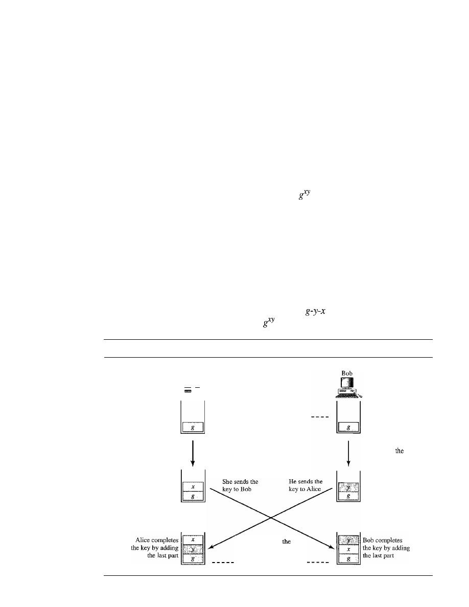
954
CHAPTER 30
CRYPTOGRAPHY
Example 30.10
Let us give a trivial example to make the procedure clear. Our example uses small num-
bers, but note that in a real situation, the numbers are very large. Assume g
=
7 and p
=
23.
The steps are as follows:
1.
Alice chooses
x
=
3 and calculates
R
1
=
7
3
mod 23
=
21.
2. Bob chooses y
=
6 and calculates
R
2
=
7
6
mod 23
=
4.
3. Alice sends the number 21 to Bob.
4. Bob sends the number 4 to Alice.
5. Alice calculates the symmetric key
K
=
4
3
mod 23
=
18.
6. Bob calculates the symmetric key
K
=
21
6
mod 23
=
18.
The value of
K
is the same for both Alice and Bob;
mod
p
=
7
18
mod 23
=
18.
Idea of Diffie-Hellman
The Diffie-Hellman concept, shown in Figure 30.27, is simple but elegant. We can think
of the secret key between Alice and Bob as made of three parts: g,
x,
and
y.
The first part
is public. Everyone knows one-third of the key;
g
is a public value. The other two parts
must be added by Alice and Bob. Each adds one part. Alice adds
x
as the second part for
Bob; Bob adds y as the second part for Alice. When Alice receives the two-thirds com-
pleted key from Bob, she adds the last part, her
x, to complete the key. When Bob receives
the two-thirds completed key from Alice, he adds the last part, his y, to complete the key.
Note that although the key in Alice's hand consists of
and the key in Bob's hand is
g-x-y,
these two keys are the same because
=
gYx.
Figure 30.27
Diffie-Hellman idea
Alice
....
Alice fills up another
one-third of the
secret key using
her random number
One-third of the key is public.
The two keys are
same
because it does not matter
if x is filled first or
y.
Bob fills up another
one-third of
secret key using
his random number
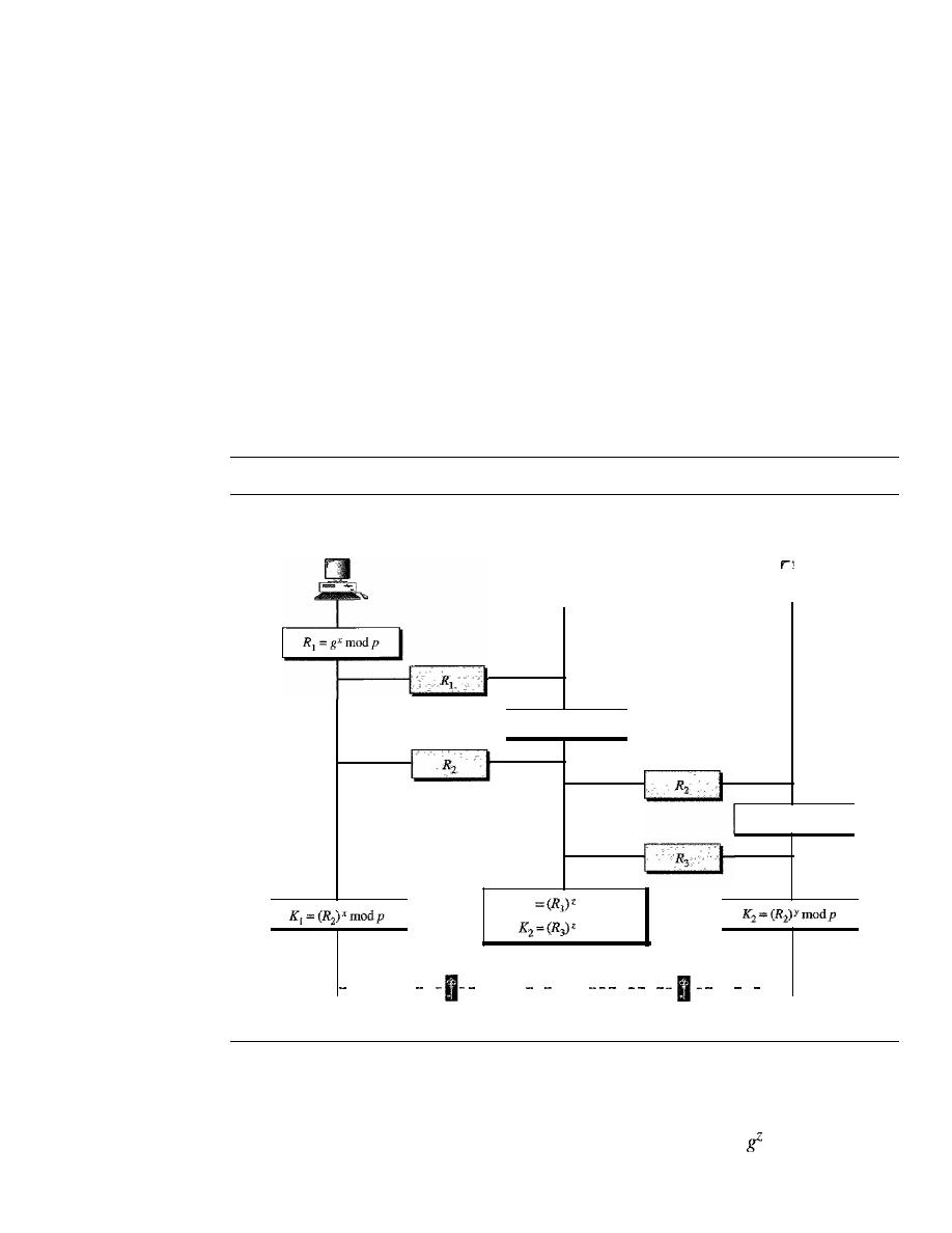
SECTION 30.3
ASYMMETRIC-KEY CRYPTOGRAPHY
955
Note also that although the two keys are the same, Alice cannot find the value y used by
Bob because the calculation is done
in
modulo p; Alice receives gY mod p from Bob, not gY.
Man-in-the-Middle Attack
Diffie-Hellman is a very sophisticated symmetric-key creation algorithm.
If
x
and
y
are
very large numbers, it is extremely difficult for Eve to find the key, knowing only
p
and
g. An intruder needs to determine x and y if
R
1
and
R
2
are intercepted. But finding x
from R
1
and
y
from R
2
are two difficult tasks. Even a sophisticated computer would
need perhaps years to find the key by trying different numbers. In addition, Alice and
Bob will change the key the next time they need to communicate.
However, the protocol does have a weakness. Eve does not have to find the value of
x
and
y
to attack the protocol. She can fool Alice and Bob by creating two keys: one
between herself and Alice and another between herself and Bob. Figure 30.28 shows
the situation.
Figure 30.28
Man-in-the-middle attack
p
and
g
are public.
Alice
Eve
R
z =gZmodp
K]
mod
p
mod
p
Bob
R
3 =gYmodp
Alice-Eve key
Eve-Bob key
------- -
----- - - -- - -
-- - ---
K
1
=gXZmodp
K
z
=
gZY modp
The following can happen:
1. Alice chooses
x,
calculates
R1
=
gX
mod
p,
and sends
R1
to Bob.
2. Eve, the intruder, intercepts
R
l'
She chooses
z,
calculates
R
2
=
mod
p,
and sends
R
2
to both Alice and Bob.

956
CHAPTER 30
CRYPTOGRAPHY
3. Bob chooses
y,
calculates R
3
=
gY
mod
p,
and sends R
3
to Alice; R
3
is intercepted
by Eve and never reaches Alice.
4. Alice and Eve calculate
K
I
=
mod
p,
which becomes a shared key between Alice
and Eve. Alice, however, thinks that it is a key shared between Bob and herself.
5. Eve and Bob calculate
K
2
=
gZY
mod p, which becomes a shared key between Eve
and Bob. Bob, however, thinks that it is a key shared between Alice and himself.
In other words, two keys, instead of one, are created: one between Alice and Eve and
one between Eve and Bob. When Alice sends data to Bob encrypted with
K
1
(shared by
Alice and Eve), it can be deciphered and read by Eve. Eve can send the message to Bob
encrypted by
K
2
(shared key between Eve and Bob); or she can even change the mes-
sage or send a totally new message. Bob is fooled into believing that the message has
come from Alice. A similar scenario can happen to Alice in the other direction.
This situation is called a man-in-the-middle attack because Eve comes in between
and intercepts R
I ,
sent by Alice to Bob, and R
3,
sent by Bob to Alice.
It
is also known
as a bucket brigade attack because it resembles a short line of volunteers passing a
bucket of water from person to person.
Authentication
The man-in-the-middle attack can be avoided if Bob and Alice first authenticate each
other. In other words, the exchange key process can be combined with an authentication
scheme to prevent a man-in-the-middle attack. We discuss authentication in Chapter 31.
30.4
RECOMMENDED READING
For more details about subjects discussed in this chapter, we recommend the following
books. The items in brackets [...] refer to the reference list at the end of the text.
Books
Cryptography can be found in many books dedicated to the subject such as [Bar02],
[GartH], [Sti02], [Mao04], [MOV97], and [Sch96].
30.5
KEY TERMS
Advanced Encryption Standard (AES)
block cipher
bucket brigade attack
Caesar cipher
cipher block chaining (CBC) mode
cipher feedback (CFB) mode
ciphertext
compression permutation
cryptography
Data Encryption Standard (DES)
decryption
decryption algorithm
DES function
Diffie-Hellman cryptosystem
electronic code book (ECB) mode
encryption

encryption algorithm
expansion permutation
initiation vector (IV)
key
man-in-the-middle attack
mode of operation
monoalphabetic cipher
National Institute of Standards and
Technology (NIST)
output feedback (OFB) mode
P-box
plaintext
polyalphabetic cipher
private key
public key
SECTION 30.6
SUMMARY
957
Rijndael algorithm
Rivest, Shamir, Adleman (RSA)
rotation cipher
round
round cipher
S-box
secret key
session key
shift cipher
simple cipher
straight permutation
substitution cipher
transposition cipher
Triple DES
XORcipher
30.6
SUMMARY
o
Cryptography is the science and art of transforming messages to make them secure
and immune to attacks.
o
The plaintext is the original message before transformation; the ciphertext is the
message after transformation.
o
An encryption algorithm transforms plaintext to ciphertext; a decryption algorithm
transforms ciphertext to plaintext.
o
A combination of an encryption algorithm and a decryption algorithm is called a
cipher.
o
The key is a number or a set of numbers on which the cipher operates.
o
We can divide all ciphers into two broad categories: symmetric-key ciphers and
asymmetric-key ciphers.
o
In a symmetric-key cipher, the same key is used by both the sender and receiver. The
key is called the secret key.
o
In an asymmetric-key cipher, a pair of keys is used. The sender uses the public key;
the receiver uses the private key.
o
A substitution cipher replaces one character with another character.
o
Substitution ciphers can be categorized into two broad categories: monoalphabetic
and polyalphabetic.
o
The shift cipher is the simplest monoalphabetic cipher.
It
uses modular arithmetic
with a modulus of 26. The Caesar cipher is a shift cipher that has a key of 3.
o
The transposition cipher reorders the plaintext characters to create a ciphertext.
o
An XOR cipher is the simplest cipher which is self-invertible.
o
A rotation cipher is an invertible cipher.

958
CHAPTER 30
CRYPTOGRAPHY
o
An S-box is a keyless substitution cipher with
N
inputs and
M
outputs that uses a
formula to define the relationship between the input stream and the output stream.
o
A P-box is a keyless transposition cipher with
N
inputs and
M
outputs that uses a
table to define the relationship between the input stream and the output stream. A
P-box is invertible only if the numbers of inputs and outputs are the same. A P-box can
use a straight permutation, a compression peilliutation, or an expansion permutation.
o
A modern cipher is usually a round cipher; each round is a complex cipher made of
a combination of different simple ciphers.
o
DES is a symmetric-key method adopted by the U.S. government. DES has an initial
and final permutation block and 16 rounds.
o
The heart of DES is the DES function. The DES function has four components: an
expansion permutation, an XOR operation, S-boxes, and a straight permutation.
o
DES uses a key generator to generate sixteen 48-bit round keys.
o
Triple DES was designed to increase the size of the DES key (effectively 56 bits)
for better security.
o
AES is a round cipher based on the Rijndael algorithm that uses a 128-bit block of
data. AES has three different configurations: 10 rounds with a key size of 128 bits,
12 rounds with a key size of 192 bits, and 14 rounds with a key size of 256 bits.
o
Mode of operation refers to techniques that deploy the ciphers such as DES or AES.
Four common modes of operation are ECB, CBC, CBF, and OFB. ECB and CBC
are block ciphers; CBF and OFB are stream ciphers.
o
One commonly used public-key cryptography method is the RSA algorithm,
invented by Rivest, Shamir, and Adleman.
o
RSA chooses n to be the product of two primes
p
and
q.
o
The Diffie-Hellman method provides a one-time session key for two parties.
o
The man-in-the-middle attack can endanger the security of the Diffie-Hellman
method if two parties are not authenticated to each other.
30.7
PRACTICE SET
Review Questions
1. In symmetric-key cryptography, how many keys are needed if Alice and Bob want
to communicate with each other?
2. In symmetric-key cryptography, can Alice use the same key to communicate with
both Bob and John? Explain your answer.
3. In symmetric-key cryptography, if every person in a group of 10 people needs to
communicate with every other person in another group of 10 people, how many
secret keys are needed?
4. In symmetric-key cryptography, if every person in a group of 10 people needs to com-
municate with every other person in the group, how many secret keys are needed?
5. Repeat Question 1 for asymmetric-key cryptography.

SECTION 30.
7
PRACTICE SET
959
6. Repeat Question 2 for asymmetric-key cryptography.
7. Repeat Question 3 for asymmetric-key cryptography.
8. Repeat Question 4 for asymmetric-key cryptography.
Exercises
9. In symmetric-key cryptography, how do you think two persons can establish a secret
key between themselves?
10. In asymmetric-key cryptography, how do you think two persons can establish two
pairs of keys between themselves?
11. Encrypt the message "THIS IS AN EXERCISE" using a shift cipher with a key of 20.
Ignore the space between words. Decrypt the message to get the original plaintext.
12. Can we use monoalphabetic substitution if our symbols are just 0 and I? Is it a
good idea?
13. Can we use polyalphabetic substitution if our symbols are just 0 and I? Is it a good
idea?
14. Encrypt "INTERNET" using a transposition cipher with the following key:
3 5 2 1 4
1 2
15. Rotate 11100 I three bits to the right.
16. Rotate 100111 three bits to the left.
17. A 6-by-2 S-box adds the bits at the odd-numbered positions
(1,
3, 5, ...) to get the
right bit of the output and adds the bits at the even-numbered positions (2,4,6, ...)
to get the left bit of the output.
If
the input is 1100 I0, what is the output? If the
input is 10 110 I, what is the output? Assume the rightmost bit is bit I.
18. What are all the possible number combinations of inputs in a 6-by-2 S-box? What
is the possible number of outputs?
19. The leftmost bit of a 4-by-3 S-box rotates the other 3 bits.
If
the leftmost bit is 0,
the 3 other bits are rotated to the right 1 bit. If the leftmost bit is I, the 3 other bits
are rotated to the left I bit.
If
the input is 10 II, what is the output?
If
the input is
0110, what is the output?
20. A P-box uses the following table for encryption. Show the box and connect the input
to the output.
4
1
3
Is the P-box straight, compression, or expansion?
21. In RSA, given two prime numbers
p
=
19 and
q
=
23, find nand
Choose
e
=
5 and
try to find
d,
such that
e
and
d
meet the criteria.
22. To understand the security of the RSA algorithm, find
d
if you know that e
=
17 and
n
=
187. This exercise proves how easy is for Eve to break the secret if
n
is small.

960
CHAPTER 30
CRYPTOGRAPHY
23. For the RSA algorithm with a large
n,
explain why Bob can calculate d from
n,
but
Eve cannot.
24. Using
e
=
13,
d
=
37, and
n
=
77 in the RSA algorithm, encrypt the message "FINE"
using the values of 00 to 25 for letters A to Z. For simplicity, do the encryption and
decryption character by character.
25. Why can't Bob choose 1 as the public key e in RSA?
26. What is the danger in choosing 2 as the public key e in RSA?
27. Eve uses RSA to send a message to Bob, using Bob's public key. Later, at a cock-
tail party, Eve sees Bob and asks him if the message has arrived and Bob confirms
it. After a few drinks, Eve asks Bob, "What was the ciphertext?" Bob gives the
value of the ciphertext to Eve. Can this endanger the security of Bob's private key?
Explain your answer.
28. What is the value of the symmetric key
in
the Diffie-Hellman protocol if
g
=
7,p
=
23,
x
=
2, and y
=
5?
29. In the Diffie-Hellman protocol, what happens if x and y have the same value? That
is, Alice and Bob have accidentally chosen the same number. Are the values of R
1
and R
2
the same? Are the values of the session keys calculated by Alice and Bob
the same? Use an example to prove your claims.
Research Activities
30. Another asymmetric-key algorithm is called EIGamal. Do some research and find
out some information about this algorithm. What is the difference between RSA
and EIGamal?
31. Another asymmetric-key algorithm is based on elliptic curves.
If
you are familiar
with elliptic curves, do some research and find the algorithms based on elliptic
curves.
32. To make Diffie-Helman algorithm more robust, one uses cookies. Do some research
and find out about the use of cookies in the Diffie-Helman algorithm.
CHAPTER 31
Network Security
In
Chapter 30, we introduced the science of cryptography. Cryptography has several
applications in network security.
In
this chapter, we first introduce the security services
we typically expect in a network. We then show how these services can be provided
using cryptography. At the end of the chapter, we also touch on the issue of distributing
symmetric and asymmetric keys. The chapter provides the background necessary for
Chapter 32, where we discuss security in the Internet.
31.1
SECURITY SERVICES
Network security can provide one of the five services as shown in Figure 31.1. Four of
these services are related to the message exchanged using the network: message confi-
dentiality, integrity, authentication, and nonrepudiation. The fifth service provides
entity authentication or identification.
Figure 31.1
Security services related to the message or entity
Message
Security
services
Entity
Confidentiality
Integrity
Authentication
Nonrepudiatton
Authentication
961

962
CHAPTER
31
NETWORK SECURiTY
Message Confidentiality
Message confidentiality or privacy means that the sender and the receiver expect con-
fidentiality. The transmitted message must make sense to only the intended receiver. To
all others, the message must be garbage. When a customer communicates with her
bank, she expects that the communication is totally confidential.
Message Integrity
Message integrity means that the data must arrive at the receiver exactly as they were
sent. There must be no changes during the transmission, neither accidentally nor mali-
ciously. As more and more monetary exchanges occur over the Internet, integrity is crucial.
For example, it would be disastrous if a request for transferring $100 changed to a
request for $10,000 or $100,000. The integrity of the message must be preserved in a
secure communication.
Message Authentication
Message authentication is a service beyond message integrity. In message authentication
the receiver needs to be sure of the sender's identity and that an imposter has not sent the
message.
Message Nonrepudiation
Message nonrepudiation means that a sender must not be able to deny sending a message
that he or she, in fact, did send. The burden of proof falls on the receiver. For example,
when a customer sends a message to transfer money from one account to another, the
bank must have proof that the customer actually requested this transaction.
Entity Authentication
In entity authentication (or user identification) the entity or user is verified prior to
access to the system resources (files, for example). For example, a student who needs to
access her university resources needs to be authenticated during the logging process.
This is to protect the interests of the university and the student.
31.2
MESSAGE CONFIDENTIALITY
The concept of how to achieve message confidentiality or privacy has not changed for
thousands of years. The message must be encrypted at the sender site and decrypted
at the receiver site. That is, the message must be rendered unintelligible to unauthorized
parties. A good privacy technique guarantees to some extent that a potential intruder
(eavesdropper) cannot understand the contents of the message. As we discussed in
Chapter 30, this can be done using either symmetric-key cryptography or asymmetric-
key cryptography. We review both.
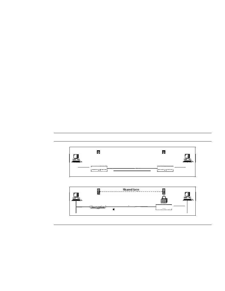
SECTION
31.2
MESSAGE CONFIDENTIALITY
963
Confidentiality with Symmetric-Key Cryptography
Although modern symmetric-key algorithms are more complex than the ones used
through the long history of the secret writing, the principle is the same. To provide confi-
dentiality with symmetric-key cryptography, a sender and a receiver need to share a
secret key. In the past when data exchange was between two specific persons (for exam-
ple, two friends or a ruler and her army chief), it was possible to personally exchange the
secret keys. Today's communication does not often provide this opportunity. A person
residing in the United States cannot meet and exchange a secret key with a person living
in China. Furthermore, the communication is between millions of people, not just a few.
To be able to use symmetric-key cryptography, we need to find a solution to the
key sharing. This can be done using a session key. A session key is one that is used only
for the duration of one session. The session key itself is exchanged using asymmetric-
key cryptography as we will see later. Figure 31.2 shows the use of a session symmetric
key for sending confidential messages from Alice to Bob and vice versa. Note that the
nature of the symmetric key allows the communication to be carried on in both direc-
tions although it is not recommended today. Using two different keys is more secure,
because if one key is compromised, the communication is still confidential in the other
direction.
Figure 31.2
Message confidentiality using symmetric keys in two directions
Alice
Shared keys
mr-----------------------------lI
Bob
Plaintext
Ciphertext
Plaintext
Data flow
a. A shared secret key can be used in Alice-Bob communication
Alice
Plaintext
Ciphertext
Plaintext
Data flow
b. A different shared secret key is recommended in Bob-Alice communication
Bob
The reason symmetric-key cryptography is still the dominant method for confiden-
tiality of the message is its efficiency. For a long message, symmetric-key cryptography
is much more efficient than asymmetric-key cryptography.
Confidentiality with Asymmetric-Key Cryptography
The problem we mentioned about key exchange in symmetric-key cryptography for
privacy culminated in the creation of asymmetric-key cryptography. Here, there is no
key sharing; there is a public announcement. Bob creates two keys: one private and one
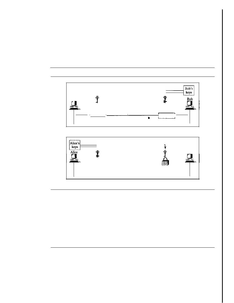
964
CHAPTER
31
NETWORK SECURITY
public. He keeps the private key for decryption; he publicly announces the public key to
the world. The public key is used only for encryption; the private key is used only for
decryption. The public key locks the message; the private key unlocks it.
For a two-way communication between Alice and Bob, two pairs of keys are
needed. When Alice sends a message to Bob, she uses Bob's pair; when Bob sends a
message to Alice, he uses Alice's pair as shown in Figure 31.3.
Figure 31.3
Message confidentiality using asymmetric keys
Alice
- - - - - - - - - - - - -
f
f
Plaintext
I
. I
Ciphertext
Plaintext
Encryption
Data flow
a. Bob's keys are used in Alice-Bob communication
- - - - - - - - - - - - -
t
Data flow
b. Alice's keys are used in Bob·Alice communication
Bob
Confidentiality with asymmetric-key cryptosystem has its own problems. First, the
method is based on long mathematical calculations using long keys. This means that
this system is very inefficient for long messages; it should be applied only to short mes-
sages. Second, the sender of the message still needs to be certain about the public key
of the receiver. For example, in Alice-Bob communication, Alice needs to be sure that
Bob's public key is genuine; Eve may have announced her public key in the name of
Bob. A system of trust is needed, as we will see later in the chapter.
31.3
MESSAGE INTEGRITY
Encryption and decryption provide secrecy, or confidentiality, but not
integrity.
How-
ever, on occasion we may not even need secrecy, but instead must have integrity. For
example, Alice may write a will to distribute her estate upon her death. The will does
not need to be encrypted. After her death, anyone can examine the will. The integrity of
the will, however, needs to be preserved. Alice does not want the contents of the will to
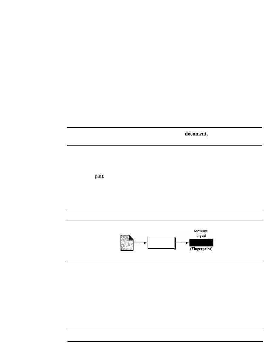
SECTION
31.3
MESSAGE INTEGRITY
965
be changed. As another example, suppose Alice sends a message instructing her banker,
Bob, to pay Eve for consulting work. The message does not need to be hidden from Eve
because she already knows she is to be paid. However, the message does need to be safe
from any tampering, especially by Eve.
Document and Fingerprint
One way to preserve the integrity of a document is through the use of a
fingerprint.
If
Alice needs to be sure that the contents of her document will not be illegally changed,
she can put her fingerprint at the bottom of the document. Eve cannot modify the contents
of this document or create a false document because she cannot forge Alice's finger-
print. To ensure that the document has not been changed, Alice's fingerprint on the doc-
ument can be compared to Alice's fingerprint on file.
If
they are not the same, the
document is not from Alice.
To preserve the integrity of a
both the document and the fingerprint are needed.
Message and Message Digest
The electronic equivalent of the document and fingerprint pair is the message and mes-
sage digest
To preserve the integrity of a message, the message is passed through
an algorithm called a
hash function.
The hash function creates a compressed image of
the message that can be used as a fingerprint. Figure 31.4 shows the message, hash
function, and the message digest.
Figure 31.4
Message and message digest
Message
(Document)
Hash
function
Difference
The two pairs document/fingerprint and message/message digest are similar, with some
differences. The document and fingerprint are physically linked together; also, neither
needs to be kept secret. The message and message digest can be unlinked (or sent) sep-
arately and, most importantly, the message digest needs to be kept secret. The message
digest is either kept secret in a safe place or encrypted if we need to send it through a
communications channel.
The message digest needs to be kept secret.
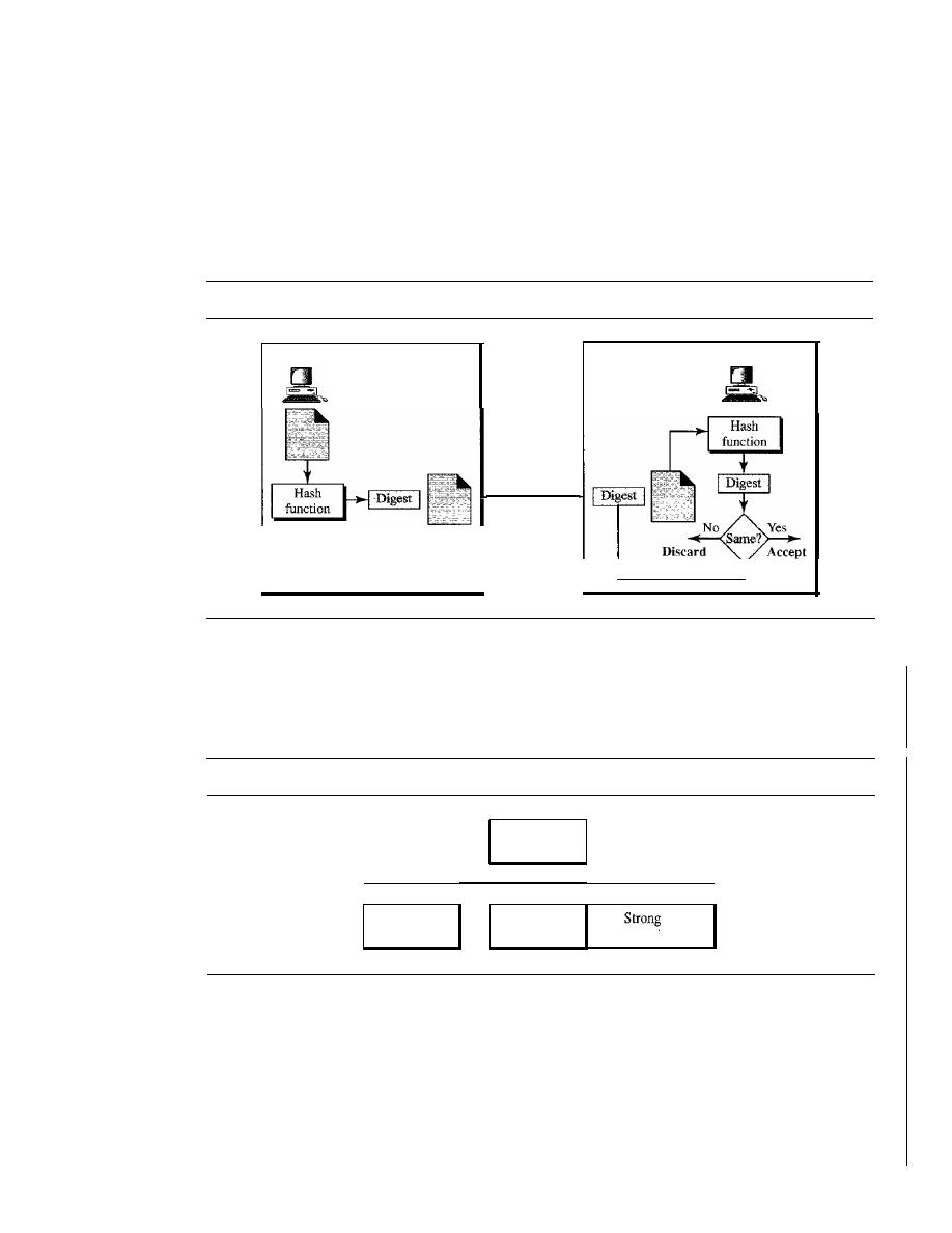
966
CHAPTER
31
NETWORK SECURITY
Creating and Checking the Digest
The message digest is created at the sender site and is sent with the message to the
receiver. To check the integrity of a message, or document, the receiver creates the hash
function again and compares the new message digest with the one received.
If
both are
the same, the receiver is sure that the original message has not been changed. Of course,
we are assuming that the digest has been sent secretly. Figure 31.5 shows the idea.
Figure 31.5
Checking integrity
Alice
Hash Function Criteria
Message
and
digest
Bob
To be eligible for a hash, a function needs to meet three criteria: one-wayness, resis-
tance to weak collision, and resistance to strong collision as shown in Figure 31.6.
Figure 31.6
Criteria of a hash function
Hash function
criteria
I
I
I
I
Onc-wayncss
Weak collision
I
collision
resistance
resistance
One-wayness
A hash function must have one-wayness; a message digest is created by a one-way
hashing function. We must not be able to recreate the message from the digest. Some-
times it is difficult to make a hash function 100 percent one-way; the criteria state that it
must be extremely difficult or impossible to create the message if the message digest is
given. This is similar to the document/fingerprint case. No one can make a document
from a fingerprint.

SECTION 31.3
MESSAGE INTEGRITY
967
Example 31.1
Can we use a conventional lossless compression method as a hashing function?
Solution
We cannot. A lossless compression method creates a compressed message that is reversible. You
can uncompress the compressed message to get the original one.
Example 31.2
Can we use a checksum method as a hashing function?
Solution
We can. A checksum function is not reversible; it meets the first criterion. However, it does not
meet the other criteria.
Weak Collision Resistance
The second criterion, weak collision resistance, ensures that a message cannot easily
be forged.
If
Alice creates a message and a digest and sends both to Bob, this criterion
ensures that Eve cannot easily create another message that hashes exactly to the same
digest. In other words, given a specific message and its digest, it is impossible (or at
least very difficult) to create another message with the same digest.
When two messages create the same digest, we say there is a collision. In a week
collision, given a message digest, it is very unlikely that someone can create a message
with exactly the same digest. A hash function must have weak collision resistance.
Strong Collision Resistance
The third criterion, strong collision resistance, ensures that we cannot find two messages
that hash to the same digest. This criterion is needed to ensure that Alice, the sender of the
message, cannot cause problems by forging a message.
If
Alice can create two messages
that hash to the same digest, she can deny sending the first to Bob and claim that she sent
only the second.
This type of collision is called strong because the probability of collision is higher
than in the previous case. An adversary can create two messages that hash to the same
digest. For example, if the number of bits in the message digest is small, it is likely
Alice can create two different messages with the same message digest. She can send the
first to Bob and keep the second for herself. Alice can later say that the second was
the original agreed-upon document and not the first.
Suppose two different wills can be created that hash to the same digest. When the
time comes for the execution of the will, the second will is presented to the heirs. Since
the digest matches both wills, the substitution is successful.
Hash Algorithms: SHA-l
While many hash algorithms have been designed, the most common is SHA-l. SHA-1
(Secure Hash Algorithm 1) is a revised version of SHA designed by the National
Institute of Standards and Technology (NIST).
It
was published as a Federal Information
Processing Standard (PIPS).
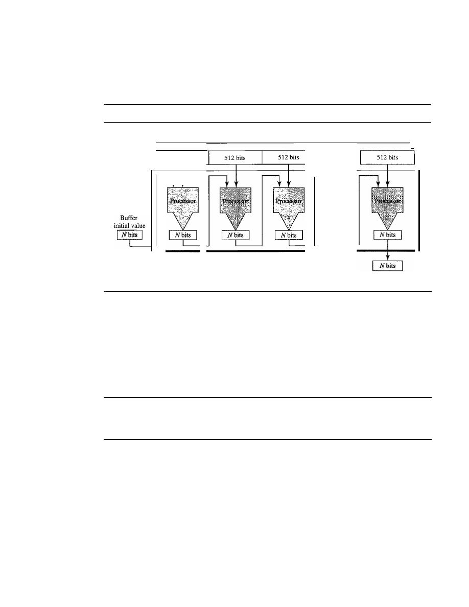
968
CHAPTER
31
NETWORK SECURITY
A very interesting point about this algorithm and others is that they all follow the
same concept. Each creates a digest of length
N
from a multiple-block message. Each
block is 512 bits in length, as shown in Figure 31.7.
Figure 31.7
Message digest creation
512 bits
Message, multiple 5l2-bit blocks
•••
.
..
..
.
Message digest
·1
A buffer of
N
bits is initialized to a predetermined value. The algorithm mangles
this initial buffer with the first 512 bits of the message to create the first intermediate
message digest of
N
bits. This digest is then mangled with the second 512-bit block to
create the second intermediate digest. The (n - l)th digest is mangled with the nth block
to create the nth digest.
If
a block is not 512 bits, padding (Os) is added to make it so.
When the last block is processed, the resulting digest is the message digest for the
entire message. SHA-l has a message digest of 160 bits (5 words, each of 32 bits).
SHA-l hash algorithms create anN-bit message
digest out of a message of 512-bit blocks.
SHA-l has a message digest of 160 bits (5 words of 32 bits).
Word Expansion
Before processing, the block needs to be expanded. A block is made of 512 bits or 16
32-bit words, but we need 80 words in the processing phase. So the 16-word block needs
to be expanded to 80 words, wordO to word79.
Processing Each Block
Figure 31.8 shows the general outline for the processing of one block. There are 80 steps
in block processing. In each step, one word from the expanded block and one 32-bit
constant are mangled together and then operated on to create a new digest. At the
beginning of processing, the values of digest words (A, B, C, D, and E) are saved into
five temporary variables. At the end of the processing (after step 79), these values are
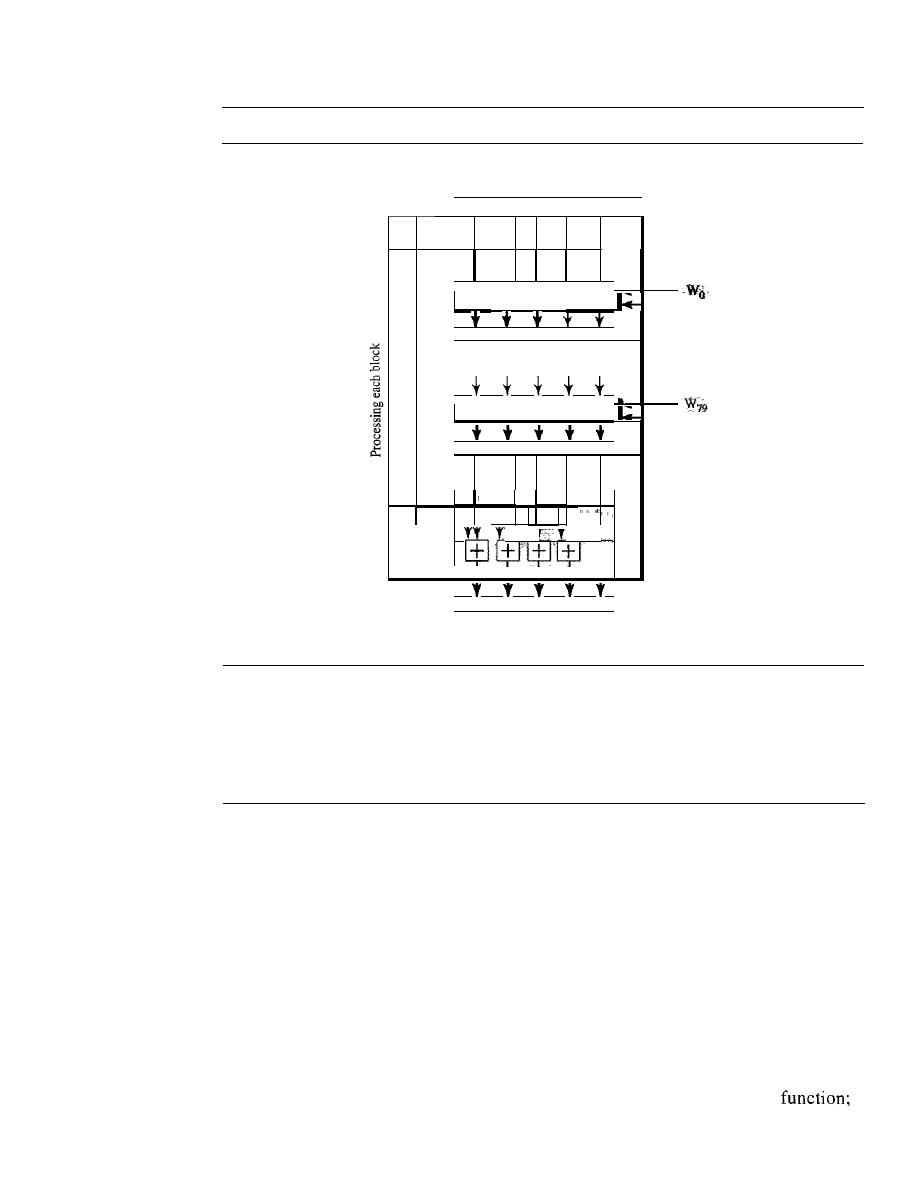
SECTION
31.4
MESSAGE AUTHENTICATION
969
Figure 31.8
Processing of one block in SHA-1
Results of the previous block
or the initial digest
IAIBICIDtE I
•
Step 0
K
o
IAIBjCtDIEI
·
•
·
Step 79
K
79
IAIBICIDIEI
Final
adding
+
l:!:J
IAIBIC/DIE
Values for the next block
or the final digest
added to the values created from step 79. The detail of each step is complex and beyond
the scope of this book. The only thing we need to know is that each step mangles a
word of data and a constant to create a result that is fed to the next step.
31.4
MESSAGE AUTHENTICATION
A hash function guarantees the integrity of a message.
It
guarantees that the message has
not been changed. A hash function, however, does not authenticate the sender of the mes-
sage. When Alice sends a message to Bob, Bob needs to know if the message is coming
from Alice or Eve. To provide message authentication, Alice needs to provide proof that
it is Alice sending the message and not an imposter. A hash function per se cannot
provide such a proof. The digest created by a hash function is normally called a
modifi-
cation detection code
(MDC). The code can detect any modification in the message.
MAC
To provide message authentication, we need to change a modification detection code to
a
message authentication code
(MAC). An MDC uses a keyless hash
a
MAC uses a keyed hash function. A keyed hash function includes the symmetric key
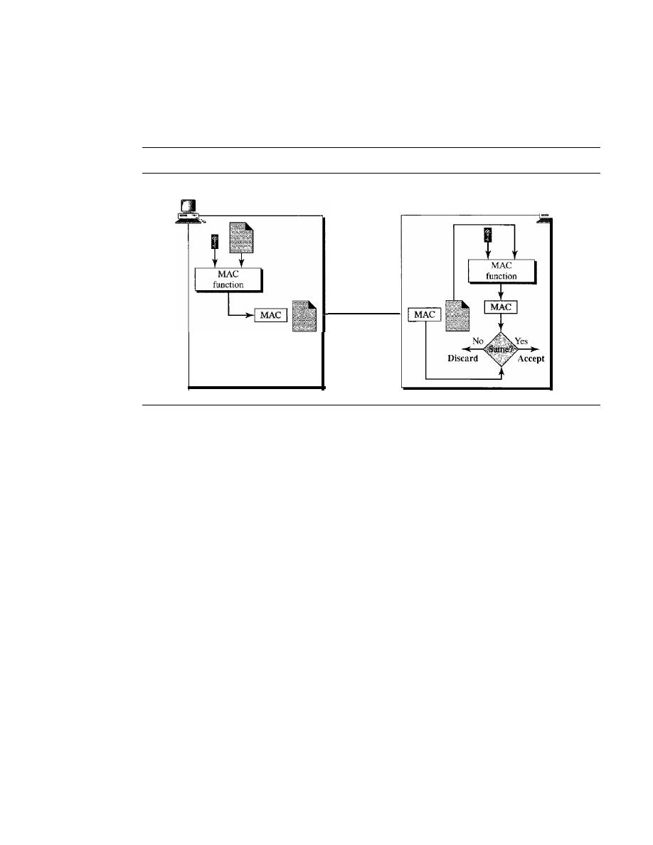
970
CHAPTER
31
NETWORK SECURITY
between the sender and receiver when creating the digest. Figure 31.9 shows how Alice
uses a keyed hash function to authenticate her message and how Bob can verify the
authenticity of the message.
Figure 31.9
MAC, created by Alice and checked by Bob
Alice
Bob
Message
and
MAC
Alice, using the symmetric key between herself and Bob
(K
AB)
and a keyed hash
function, generates a MAC. She then concatenates the MAC with the original message
and sends the two to Bob. Bob receives the message and the MAC. He separates the
message from the MAC. He applies the same keyed hash function to the message using
the symmetric key
K
AB
to get a fresh MAC. He then compares the MAC sent by Alice
with the newly generated MAC.
If
the two MACs are identical, the message has not been
modified and the sender of the message is definitely Alice.
HMAC
There are several implementations of MAC in use today. However, in recent 'years,
some MACs have been designed that are based on keyless hash functions such as
SHA-l. This idea is a hashed
MAC,
called
HMAC,
that can use any standard keyless
hash function such as SHA-l. HMAC creates a nested MAC by applying a keyless
hash function to the concatenation of the message and a symmetric key. Figure 31.10
shows the general idea.
A copy of the symmetric key is prepended to the message. The combination is
hashed using a keyless hash function, such as SHA-1. The result of this process is an
intermediate HMAC which is again prepended with the key (the same key), and the
result is again hashed using the same algorithm. The final result is an HMAC.
The receiver receives this final HMAC and the message. The receiver creates its
own HMAC from the received message and compares the two HMACs to validate the
integrity of the message and authenticate the data origin. Note that the details of an
HMAC can be more complicated than what we have shown here.
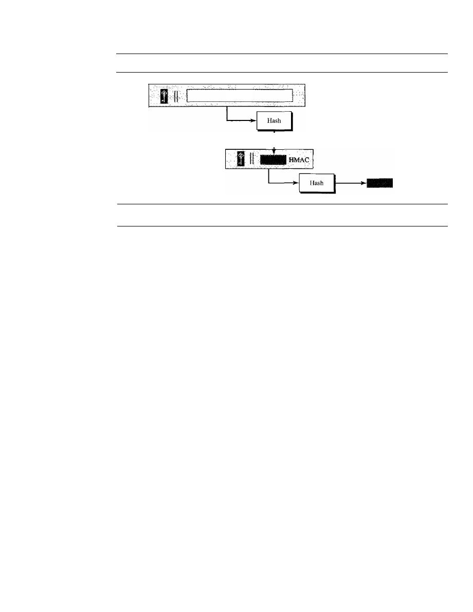
SECTION 31.5
DIGITAL SIGNATURE
971
Figure 31.10
HMAC
Message
HMAC
31.5
DIGITAL SIGNATURE
Although a MAC can provide message integrity and message authentication,
it
has a
drawback.
It
needs a symmetric key that must be established between the sender and
the receiver. A digital signature, on the other hand, can use a pair of asymmetric keys (a
public one and a private one).
We are all familiar with the concept of a signature. We sign a document to show
that it originated from us or was approved by us. The signature is proof to the recipient
that the document comes from the correct entity. When a customer signs a check to
himself, the bank needs to be sure that the check is issued by that customer and nobody
else. In other words, a signature on a document, when verified, is a sign of authentica-
tion; the document is authentic. Consider a painting signed by an artist. The signature
on the art, if authentic, means that the painting is probably authentic.
When Alice sends a message to Bob, Bob needs to check the authenticity of the
sender; he needs to be sure that the message comes from Alice and not Eve. Bob can ask
Alice to sign the message electronically. In other words, an electronic signature can
prove the authenticity of Alice as the sender of the message. We refer to this type of sig-
nature as a digital signature.
Comparison
Before we continue any further, let us discuss the differences between two types of sig-
natures: conventional and digital.
Inclusion
A conventional signature is included in the document; it is part of the document. When
we write a check, the signature is on the check;
it
is not a separate document. On the
other hand, when we sign a document digitally, we send the signature as a separate doc-
ument. The sender sends two documents: the message and the signature. The recipient
receives both documents and verifies that the signature belongs to the supposed sender.
If
this is proved, the message is kept; otherwise, it is rejected.

972
CHAPTER
31
NETWORK SECURITY
Verification Method
The second difference between the two types of documents is the method of verifying
the signature. In conventional signature, when the recipient receives a document, she
compares the signature on the document with the signature on file.
If
they are the same,
the document is authentic. The recipient needs to have a copy of this signature on file
for comparison. In digital signature, the recipient receives the message and the signa-
ture. A copy of the signature is not stored anywhere. The recipient needs to apply a
verification technique to the combination of the message and the signature to verify the
authenticity.
Relationship
In conventional signature, there is normally a one-to-many relationship between a sig-
nature and documents. A person, for example, has a signature that is used to sign many
checks, many documents, etc. In digital signature, there is a one-to-one relationship
between a signature and a message. Each message has its own signature. The signature
of one message cannot be used in another message.
If
Bob receives two messages, one
after another, from Alice, he cannot use the signature of the first message to verify the
second. Each message needs a new signature.
Duplicity
Another difference between the two types of signatures is a quality called duplicity. In
conventional signature, a copy of the signed document can be distinguished from the
original one on file. In digital signature, there is no such distinction unless there is a
factor of time (such as a timestamp) on the document. For example, suppose Alice
sends a document instructing Bob to pay Eve.
If
Eve intercepts the document and the
signature, she can resend it later to get money again from Bob.
Need for Keys
In conventional signature a signature is like a private "key" belonging to the signer of
the document. The signer uses it to sign a document; no one else has this signature. The
copy of the signature is on file like a public key; anyone can use it to verify a document,
to compare it to the original signature.
In digital signature, the signer uses her private key, applied to a signing algorithm,
to sign the document. The verifier, on the other hand, uses the public key of the signer,
applied to the verifying algorithm, to verify the document.
Can we use a secret (symmetric) key to both sign and verify a signature? The answer
is no for several reasons. First, a secret key is known only between two entities (Alice
and Bob, for example). So if Alice needs to sign another document and send it to Ted,
she needs to use another secret key. Second, as we will see, creating a secret key for a
session involves authentication, which normally uses digital signature. We have a vicious
cycle. Third, Bob could use the secret key between himself and Alice, sign a document,
send it to Ted, and pretend that it came from Alice.
A digital signature needs a public-key system.
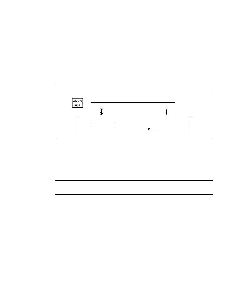
SECTION
31.5
DIGITAL SIGNATURE
973
Process
Digital signature can be achieved in two ways: signing the document or signing a digest
of the document.
Signing the Document
Probably, the easier, but less efficient way is to sign the document itself. Signing a doc-
ument is encrypting it with the private key of the sender; verifying the document is
decrypting it with the public key of the sender. Figure 31.11 shows how signing and
verifying are done.
Figure 31.11
Signing the message itself in digital signature
t
t
keys
Alice
Bob
Plaintext
Signed document
Plaintext
Encryption
Decryption
Signing
Data flow
Verifying
We should make a distinction between private and public keys as used in digital
signature and public and private keys as used for confidentiality. In the latter, the private
and public keys of the receiver are used in the process. The sender uses the public key
of the receiver to encrypt; the receiver uses his own private key to decrypt. In digital
signature, the private and public keys of the sender are used. The sender uses her pri-
vate key; the receiver uses the public key of the sender.
In a cryptosystem, we use the private and public keys of the receiver;
in digital signature, we use the private and public key of the sender.
Signing the Digest
We mentioned that the public key is very inefficient in a cryptosystem if we are dealing
with long messages. In a digital signature system, our messages are normally long, but
we have to use public keys. The solution is not to sign the message itself; instead, we
sign a digest of the message. As we learned, a carefully selected message digest has a
one-to-one relationship with the message. The sender can sign the message digest, and
the receiver can verify the message digest. The effect is the same. Figure 31.12 shows
signing a digest in a digital signature system.
A digest is made out of the message at Alice's site. The digest then goes through
the signing process using Alice's private key. Alice then sends the message and the sig-
nature to Bob. As we will see later in the chapter, there are variations in the process that
are dependent on the system. For example, there might be additional calculations before
the digest is made or other secret keys might be used. In some systems, the signature is
a set of values.
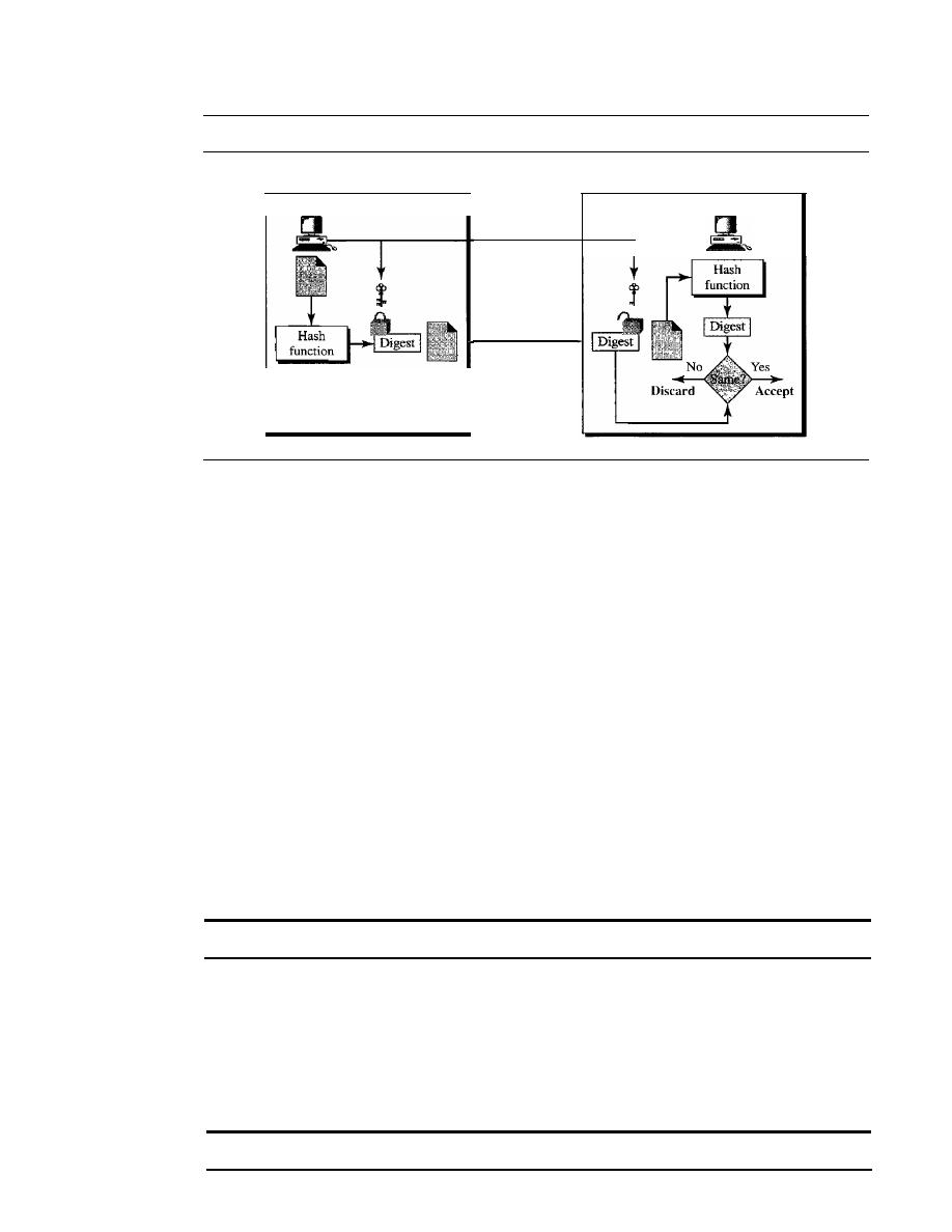
974
CHAPTER 31
NETWORK SECURITY
Figure 31.12
Signing the digest in a digital signature
Sign
Alice
Message
and
signature
Verify
Bob
At Bob's site, using the same public hash function, a digest is first created out of
the received message. Calculations are done on the signature and the digest. The verifying
process also applies criteria on the result of the calculation to detennine the authenticity
of the signature.
If
authentic, the message is accepted; otherwise, it is rejected.
Services
A digital signature can provide three out of the five services we mentioned for a security
system: message integrity, message authentication, and nonrepudiation. Note that a dig-
ital signature scheme does not provide confidential communication. If confidentiality is
required, the message and the signature must be encrypted using either a secret-key or
public-key cryptosystem.
Message Integrity
The integrity of the message is preserved even if we sign the whole message because
we cannot get the same signature if the message is changed. The signature schemes today
use a hash function in the signing and verifying algorithms that preserve the integrity of
the message.
A
digital
signature today provides message integrity.
Message Authentication
A secure signature scheme, like a secure conventional signature (one that cannot be
easily copied), can provide message authentication. Bob can verify that the message is
sent by Alice because Alice's public key is used in verification. Alice's public key cannot
create the same signature as Eve's private key.
Digital signature provides message authentication.
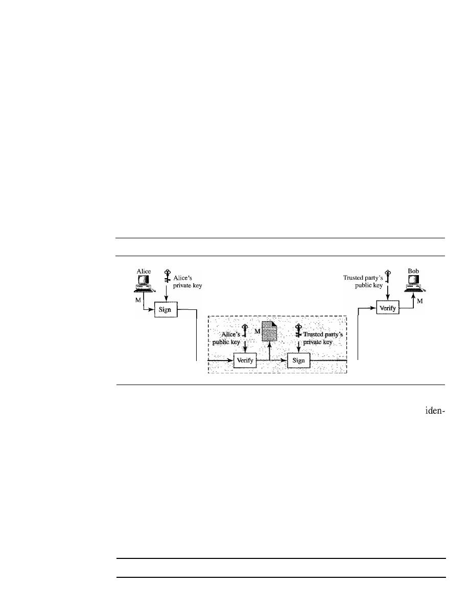
SECTION
31.5
DIGITAL SIGNATURE
975
Message Nonrepudiation
If
Alice signs a message and then denies it, can Bob later prove that Alice actually
signed it? For example, if Alice sends a message to a bank (Bob) and asks to transfer
$10,000 from her account to Ted's account, can Alice later deny that she sent this
message? With the scheme we have presented so far, Bob might have a problem.
Bob must keep the signature on file and later use Alice's public key to create the
original message to prove the message in the file and the new ly created message are
the same. This is not feasible because Alice may have changed her private/public
key during this time; she may also claim that the file containing the signature is not
authentic.
One solution is a trusted third party. People can create a trusted party among them-
selves. In Chapter 32, we will see that a trusted party can solve many other problems
concerning security services and key exchange. Figure 31.13 shows how a trusted party
can prevent Alice from denying that she sent the message.
Figure 31.13
Using a trusted center for nonrepudiation
Alice, Bob,
M,SA
M: Message
SA: Signature from Alice
ST: Signature from trusted center
Trusted center
Alice, Bob,
M,ST
Alice creates a signature from her message
(SA)
and sends the message, her
tity, Bob's identity, and the signature to the center. The center, after checking that
Alice's public key is valid, verifies through Alice's public key that the message comes
from Alice. The center then saves a copy of the message with the sender identity, recip-
ient identity, and a timestamp in its archive. The center uses its private key to create
another signature
(ST)
from the message. The center then sends the message, the new
signature, Alice's identity, and Bob's identity to Bob. Bob verifies the message using
the public key of the trusted center.
If
in the future Alice denies that she has sent the message, the center can show a
copy of the saved message. If Bob's message is a duplicate of the message saved at the
center, Alice will lose the dispute. To make everything confidential, a level of encryption!
decryption can be added to the scheme as discussed in the next section.
Nonrepudiation can be provided using a trusted party.

976
CHAPTER
31
NETWORK SECURITY
Signature Schemes
Several signature schemes have evolved during the last few decades. Some of them
have been implemented. Such as RSA and DSS (Digital Signature Standard) schemes.
The latter will probably become the standard. However, the details of these schemes are
beyond the scope of this book.
31.6
ENTITY AUTHENTICATION
Entity authentication is a technique designed to let one party prove the identity of
another party. An
entity can be a person, a process, a client, or a server. The entity
whose identity needs to be proved is called the
claimant;
the party that tries to prove
the identity of the claimant is called the
verifier.
When Bob tries to prove the identity of
Alice, Alice is the claimant, and Bob is the verifier.
There are two differences between message authentication and
entity authentication.
First, message authentication may not happen in real time; entity authentication does.
In the former, Alice sends a message to Bob. When Bob authenticates the message, Alice
mayor may not be present in the communication process. On the other hand, when
Alice requests entity authentication, there is no real message communication involved
until Alice is authenticated by Bob. Alice needs to be online and takes part in the process.
Only after she is authenticated can messages be communicated between Alice and Bob.
Message authentication is required when an e-mail is sent from Alice to Bob. Entity
authentication is required when Alice gets cash from an automatic teller machine. Second,
message authentication simply authenticates one message; the process needs to be
repeated for each new message. Entity authentication authenticates the claimant for the
entire duration of a session.
In
entity authentication, the claimant must identify herself to the verifier. This can be
done with one of three kinds of witnesses:
something known, something possessed, or
something inherent.
o
Something known.
This is a secret known only by the claimant that can be checked
by the verifier. Examples are a password, a PIN number, a secret key, and a private key.
o
Something possessed.
This is something that can prove the claimant's identity.
Examples are a passport, a driver's license, an identification card, a credit card, and
a smart card.
o
Something inherent.
This is an inherent characteristic of the claimant. Examples
are conventional signature, fingerprints, voice, facial characteristics, retinal pattern,
and handwriting.
Passwords
The simplest and the oldest method of entity authentication is the
password,
something
that the claimant
possesses. A password is used when a user needs to access a system to
use the system's resources (log-in). Each user has a user identification that is public and
a password that is private. We can divide this authentication scheme into two separate
groups: the
fixed password
and the
one-time password.

SECTION
31.6
ENTITY AUTHENTICATION
977
Fixed Password
In this group, the password is fixed; the same password is used over and over for every
access. This approach is subject to several attacks.
o
Eavesdropping.
Eve can watch Alice when she types her password. Most systems,
as a security measure, do not show the characters a user types. Eavesdropping can
take a more sophisticated form. Eve can listen to the line and then intercept the
message, thereby capturing the password for her own use.
o
Stealing a Password.
The second type of attack occurs when Eve tries to physically
steal Alice's password. This can be prevented if Alice does not write down the
password; instead, she just commits it to memory. Therefore, a password should be
very simple or else related to something familiar to Alice, which makes the password
vulnerable to other types of attacks.
o
Accessing
a
file.
Eve can hack into the system and get access to the file where the
passwords are stored. Eve can read the file and find Alice's password or even
change it. To prevent this type of attack, the file can be read/write protected. How-
ever, most systems need this type of file to be readable by the public.
o
Guessing.
Eve can log into the system and
try
to guess Alice's password by trying
different combinations of characters. The password is particularly vulnerable if the
user is allowed to choose a short password (a few characters).
It
is also vulnerable
if Alice has chosen something unimaginative, such as her birthday, her child's name,
or the name of her favorite actor. To prevent guessing, a long random password is
recommended, something that is not very obvious. However, the use of such a random
password may also create a problem; Alice might store the password somewhere
so as not to forget it. This makes the password subject to stealing.
A more secure approach is to store the hash of the password in the password file
(instead of the plaintext password). Any user can read the contents of the file, but,
because the hash function is a one-way function, it is almost impossible to guess the
value of the password. The hash function prevents Eve from gaining access to the system
even though she has the password file. However, there is a possibility of another type of
attack called the
dictionary attack.
In this attack, Eve is interested in finding one pass-
word, regardless of the user ID. For example, if the password is 6 digits, Eve can create
a list of 6-digit numbers (000000 to 999999), and then apply the hash function to every
number; the result is a list of 1 million hashes. She can then get the password file and
search the second-column entries to find a match. This could be programmed and run
offline on Eve's private computer. After a match is found, Eve can go online and use the
password to access the system. We will see how to make this attack more difficult in the
third approach.
Another approach is called
salting
the password. When the password string is created,
a random string, called the salt, is concatenated to the password. The salted password is
then hashed. The
rD,
salt, and the hash are then stored in the file. Now, when a user asks
for access, the system extracts the salt, concatenates it with the received password,
makes a hash out of the result, and compares it with the hash stored in the file.
If
there
more difficult. If the original password
is
6 digits and
the
salt
is
4 digits, then hashing

978
CHAPTER
31
NETWORK SECURITY
done over a lO-digit value. This means that Eve now needs to make a list of 10 million
items and create a hash for each of them. The list of hashes has 10 million entries and
the comparison takes much longer. Salting is very effective if the salt is a very long ran-
dom number. The UNIX operating system uses a variation of this method.
In another approach, two identification techniques are combined. A good example
of this type of authentication is the use of an ATM card with a PIN (personal identifica-
tion number). The card belongs to the category "something possessed" and the PIN
belongs to the category "something known." The PIN is actually a password that
enhances the security of the card. If the card is stolen, it cannot be used unless the PIN
is known. The PIN, however, is traditionally very short so it is easily remembered by
the owner. This makes it vulnerable to the guessing type of attack.
One-Time Password
In this type of scheme, a password is used only once. It is called the
one-time password.
A one-time password makes eavesdropping and stealing useless. However, this approach
is very complex, and we leave its discussion to some specialized books.
Challenge-Response
In password authentication, the claimant proves her identity by demonstrating that she
knows a secret, the password. However, since the claimant reveals this secret, the secret
is susceptible to interception by the adversary. In
challenge-response authentication,
the claimant proves that she knows a secret without revealing it. In other words, the
claimant does not reveal the secret to the verifier; the verifier either has it or finds it.
In challenge-response authentication,
the claimant proves that she knows a secret without revealing
it.
The challenge is a time-varying value such as a random number or a timestamp
which is sent by the verifier. The claimant applies a function to the challenge and sends
the result, called a response, to the verifier. The response shows that the claimant knows
the secret.
The challenge is a time-varying value sent by the verifier;
the response
the result of a function applied on the chanenge.
Using a Symmetric-Key Cipher
In the first category, the challenge-response authentication is achieved using symmetric-
key encryption. The secret here is the shared secret key, known by both the claimant
and the verifier. The function is the encrypting algorithm applied on the challenge.
Figure 31.14 shows one approach. The first message is not part of challenge-response,
it only informs the verifier that the claimant wants to be challenged. The second mes-
sage is the challenge. And R
B
is the nonce randomly chosen by the verifier to challenge
the claimant. The claimant encrypts the
nonce
using the shared secret key known only
to the claimant and the verifier and sends the result to the verifier. The verifier decrypts
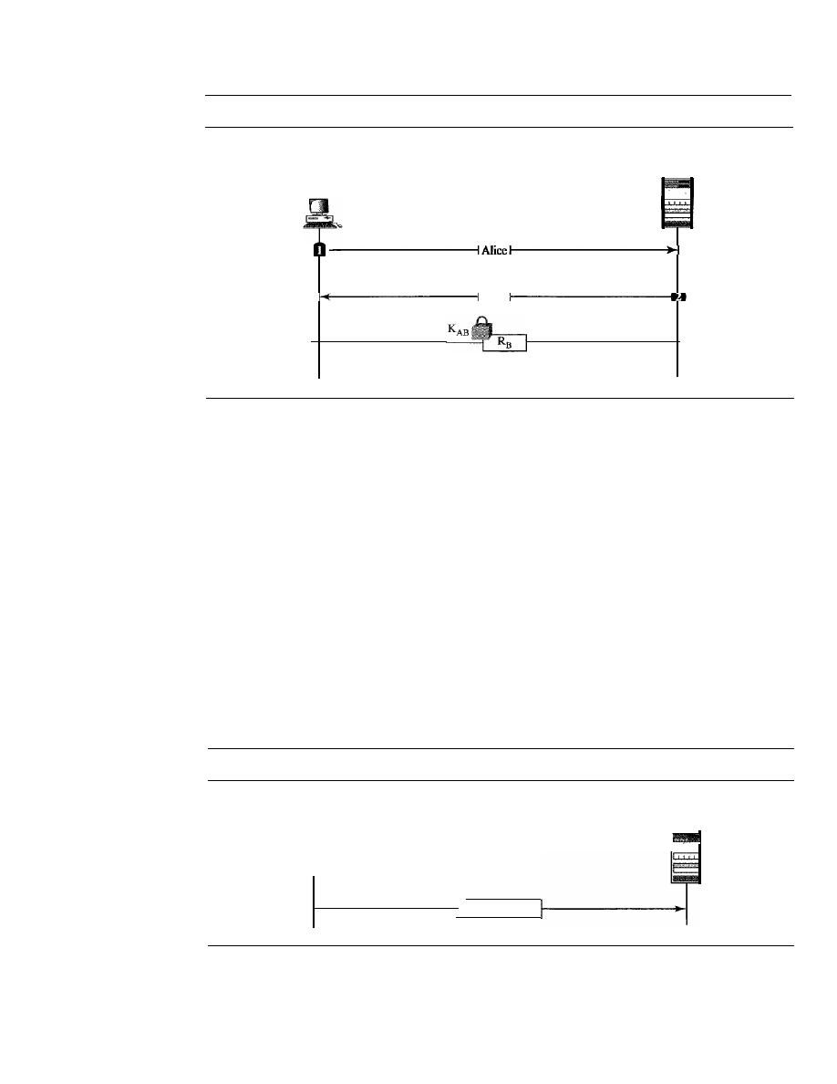
SECTION
31.6
ENTITY AUTHENTICATION
979
Figure 31.14
Challenge/response authentication using a nonce
Bob
(server)
Alice
(user)
. . .
R
B
the message. If the nonce obtained from decryption is the same as the one sent by the
verifier, Alice is granted access.
Note that in this process, the claimant and the verifier need to keep the symmetric
key used in the process secret. The verifier must also keep the value of the nonce for
claimant identification until the response is returned.
The reader may have noticed that use of a nonce prevents a replay of the third mes-
sage by Eve. Eve cannot replay the third message and pretend that it is a new request
for authentication by Alice because once Bob receives the response, the value of R
B
is
not valid any more. The next time a new value is used.
In the second approach, the time-varying value is a timestamp, which obviously
changes with time.
In this approach the challenge message is the current time sent from
the verifier to the claimant. However, this supposes that the client and the server clocks
are synchronized; the claimant knows the current time. This means that there is no need
for the challenge message. The first and third messages can be combined. The result is
that authentication can be done using one message, the response to an implicit challenge,
the current time. Figure 31.15 shows the approach.
Figure 31.15
Challenge-response authentication using a timestamp
Alice
(user)
Bob
(server)
Alice, T
Using Keyed-Hash Functions
Instead of using encryption and decryption for entity authentication, we can use a
keyed-hash function (MAC). There are two advantages to this scheme. First, the
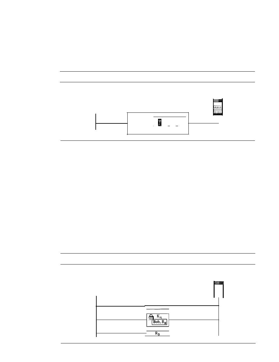
980
CHAPTER 31
NETWORK SECURITY
encryption/decryption algorithm is not exportable to some countries. Second, in using a
keyed-hash function, we can preserve the integrity of challenge and response messages
and at the same time use a secret, the key.
Let us see how we can use a keyed-hash function to create a challenge response with
a timestamp. Figure 31.16 shows the scheme.
Figure 31.16
Challenge-response authentication using a keyed-hash function
Alice
(user)
Alice, T
I
+
T
Hash
Bob
(server)
Note that in this case, the timestamp is sent both as plaintext and as text scrambled
by the keyed-hash function. When Bob receives the message, he takes the plaintext T,
applies the keyed-hash function, and then compares his calculation with what he
received to determine the authenticity of Alice.
Using an Asymmetric-Key Cipher
Instead of a symmetric-key cipher, we can use an asymmetric-key cipher for entity
authentication. Here the secret must be the private key of the claimant. The claimant
must show that she owns the private key related to the public key that is available to
everyone. This means that the verifier must encrypt the challenge using the public key
of the claimant; the claimant then decrypts the message using her private key. The
response to the challenge is the decrypted challenge. We show two approaches: one for
unidirectional authentication and one for bidirectional authentication. In one approach,
Bob encrypts the challenge using Alice's public key. Alice decrypts the message with
her private key and sends the nonce to Bob. Figure 31.17 shows this approach.
Figure 31.17
Authentication, asymmetric-key
Alice
(user)
Alice
Bob
(server)
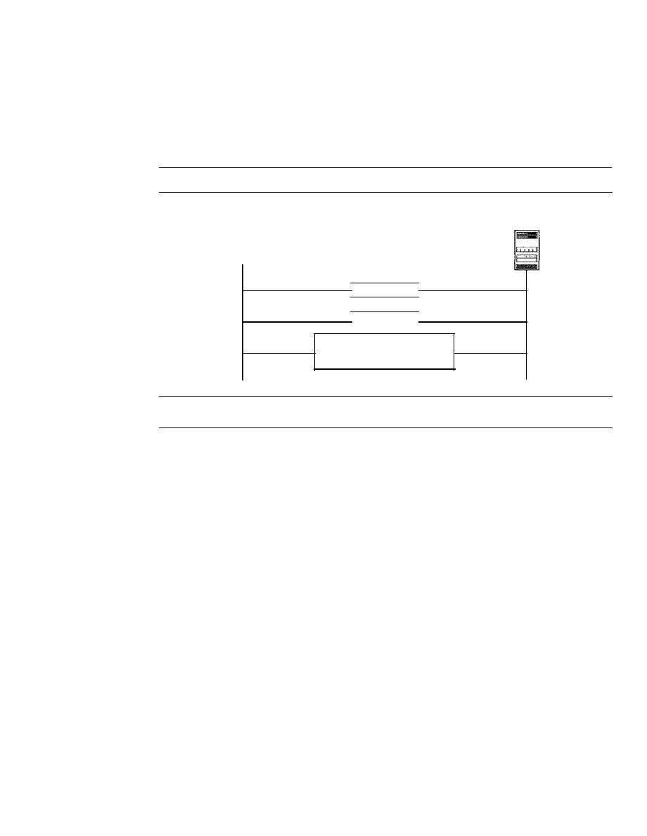
SECTION
31.7
KEY MANAGEMENT
981
Using Digital Signature
We can use digital signature for entity authentication. In this method, we let the claim-
ant use her private key for signing instead of using it for decryption. In one approach
shown in Figure 31.18, Bob uses a plaintext challenge. Alice signs the response.
Figure 31.18
Authentication, using digital signature
Alice
(user)
Alice
Bob
31.7
KEY MANAGEMENT
Bob
(server)
We have used symmetric-key and asymmetric-key cryptography in our discussion
throughout the chapter. However, we never discussed how secret keys in symmetric-key
cryptography and how public keys in asymmetric-key cryptography are distributed and
maintained. In this section, we touch on these two issues. We first discuss the distribu-
tion of symmetric keys; we then discuss the distribution of asymmetric keys.
Symmetric-Key Distribution
We have learned that symmetric-key cryptography is more efficient than asymmetric-
key cryptography when we need to encrypt and decrypt large messages. Symmetric-
key cryptography, however, needs a shared secret key between two parties.
If Alice needs to exchange confidential messages with
N
people, she needs
N
different
keys. What if
N
people need to communicate with one another? A total of
N(N -
1)/2 keys
is needed. Each person needs to have
N -
1 keys to communicate with each of the other
people, but because the keys are shared, we need only
N(N - 1)12.
This means that if
1 million people need to communicate with one another, each person has almost 0.5 mil-
lion different keys; in total, almost 1 billion keys are needed. This is normally referred to as
the
N
2
problem because the number of required keys for
N
entities is close to
N
2
.
The number of keys is not the only problem; the distribution of keys is another.
If
Alice and Bob want to communicate, they need to somehow exchange a secret key; if
Alice wants to communicate with 1 million people, how can she exchange 1 million
keys with 1 million people? Using the Internet is definitely not a secure method.
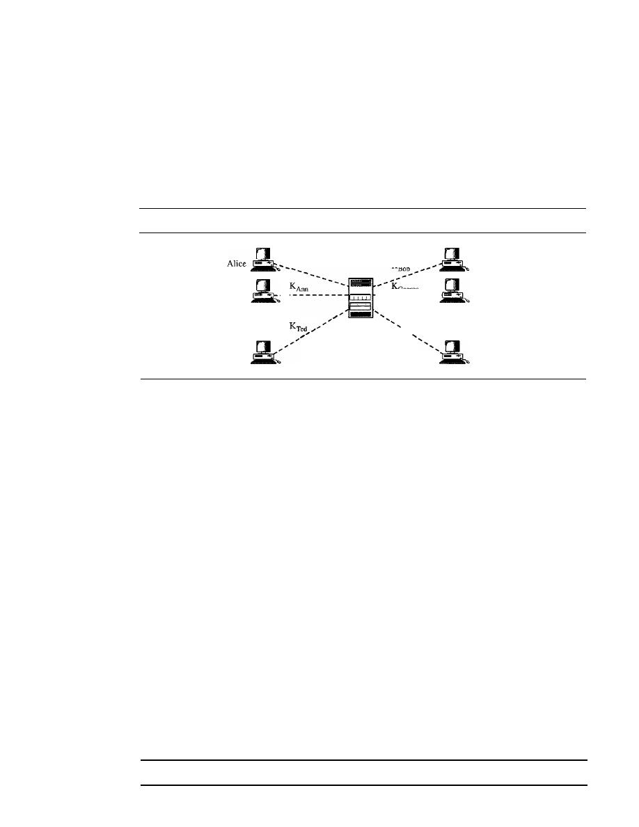
982
CHAPTER 31
NETWORK SECURITY
It
is obvious that we need an efficient way of maintaining and distributing secret
keys.
Key Distribution Center: KDC
A practical solution is the use of a trusted party, referred to as a
key distribution cen-
ter
(KDC). To reduce the number of keys, each person establishes a shared secret key
with the KDC as shown in Figure 31.19.
Figure 31.19
KDC
K
Alice
K
Bob
Bb
Ann
George
Ann
-
- - - - - - - - - -
- - - - - - - - - -
-
George
•
-
K
Betsy
:
KDC
Ie
.....
...
Ted
Betsy
A secret key is established between KDC and each member. Alice has a secret key
with KDC, which we refer to as K
Alice ;
Bob has a secret key with KDC, which we refer
to as K
Bob;
and so on. Now the question is, How can Alice send a confidential message
to Bob? The process is as follows:
1.
Alice sends a request to KDC, stating that she needs a session (temporary) secret
key between herself and Bob.
2. KDC informs Bob of Alice's request.
3. If Bob agrees, a session key is created between the two.
The secret key between Alice and Bob that is established with the KDC is used to
authenticate Alice and Bob to the KDC and to prevent Eve from impersonating either
of them. We discuss how a session key is established between Alice and Bob later in the
chapter.
Session Keys
A KDC creates a secret key for each member. This secret key can be used only between
the member and the KDC, not between two members. If Alice needs to communicate
secretly with Bob, she needs a secret key between herself and Bob. A KDC can create a
session (temporary) key between Alice and Bob using their keys with the center. The
keys of Alice and Bob are used to authenticate Alice and Bob to the center and to each
other before the session key is established. After communication is terminated, the ses-
sion key is no longer valid.
A session symmetric key between two parties is used only once.
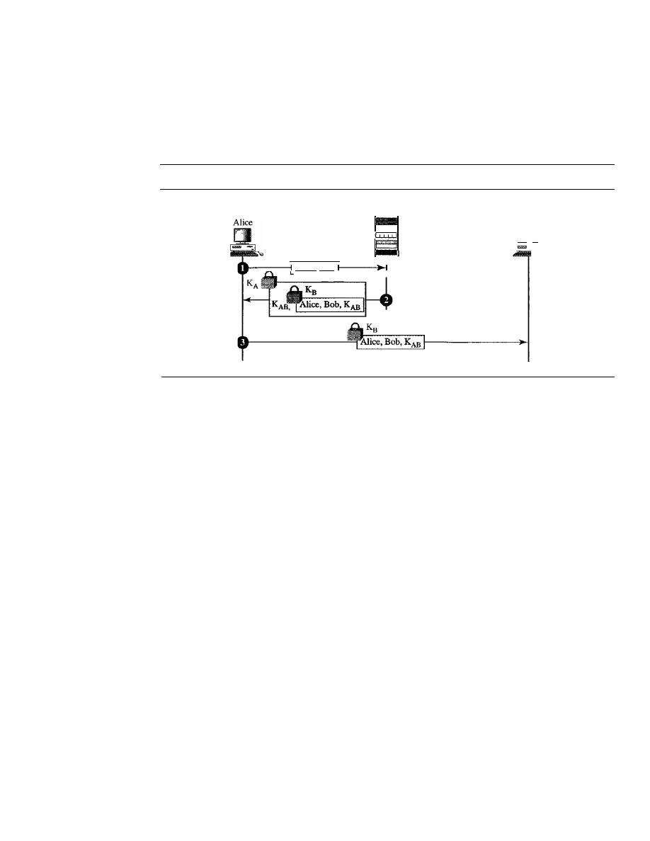
SECTION
31.7
KEY MANAGEMENT
983
Several different approaches have been proposed to create the session key using
ideas we previously discussed for entity authentication.
Let us discuss one approach, the simplest one, as shown in Figure 31.20. Although
this system has some flaws, it shows the idea. More sophisticated approaches can be
found in security books.
Figure 31.20
Creating a session key between Alice and Bob using KDC
KDC
• •
Alice, Bob
Bob
....
D
Step 1
Alice sends a plaintext message to the KDC to obtain a symmetric session
key between Bob and herself. The message contains her registered identity (the
word Alice in the figure) and the identity of Bob (the word Bob in the figure). This
message is not encrypted, it is public. KDC does not care.
D
Step
2 KDC receives the message and creates what is called a
ticket.
The ticket is
encrypted using Bob's key (K
B).
The ticket contains the identities of Alice and Bob
and the session key (K
AB ).
The ticket with a copy of the session key is sent to Alice.
Alice receives the message, decrypts it, and extracts the session key. She cannot
decrypt Bob's ticket; the ticket is for Bob, not for Alice. Note that we have a double
encryption in this message; the ticket is encrypted and the entire message is also
encrypted. In the second message, Alice is actually authenticated to the KDC,
because only Alice can open the whole message using her secret key with KDC.
D
Step
3 Alice sends the ticket to Bob. Bob opens the ticket and knows that Alice needs
to send messages to him using K
AB
as the session key. Note that in this message,
Bob is authenticated to the KDC because only Bob can open the ticket. Since Bob is
authenticated to the KDC, he is also authenticated to Alice who trusts the KDC. In
the same way, Alice is also authenticated to Bob, because Bob trusts the KDC and
the KDC has sent the ticket to Bob which includes the identity of Alice.
Kerberos
Kerberos is an authentication protocol and at the same time a KDC that has become
very popular. Several systems including Windows 2000 use Kerberos. It is named after
the three-headed dog in Greek mythology that guards the Gates of Hades. Originally
designed at M.LT., it has gone through several versions. We discuss only version 4, the
most popular.
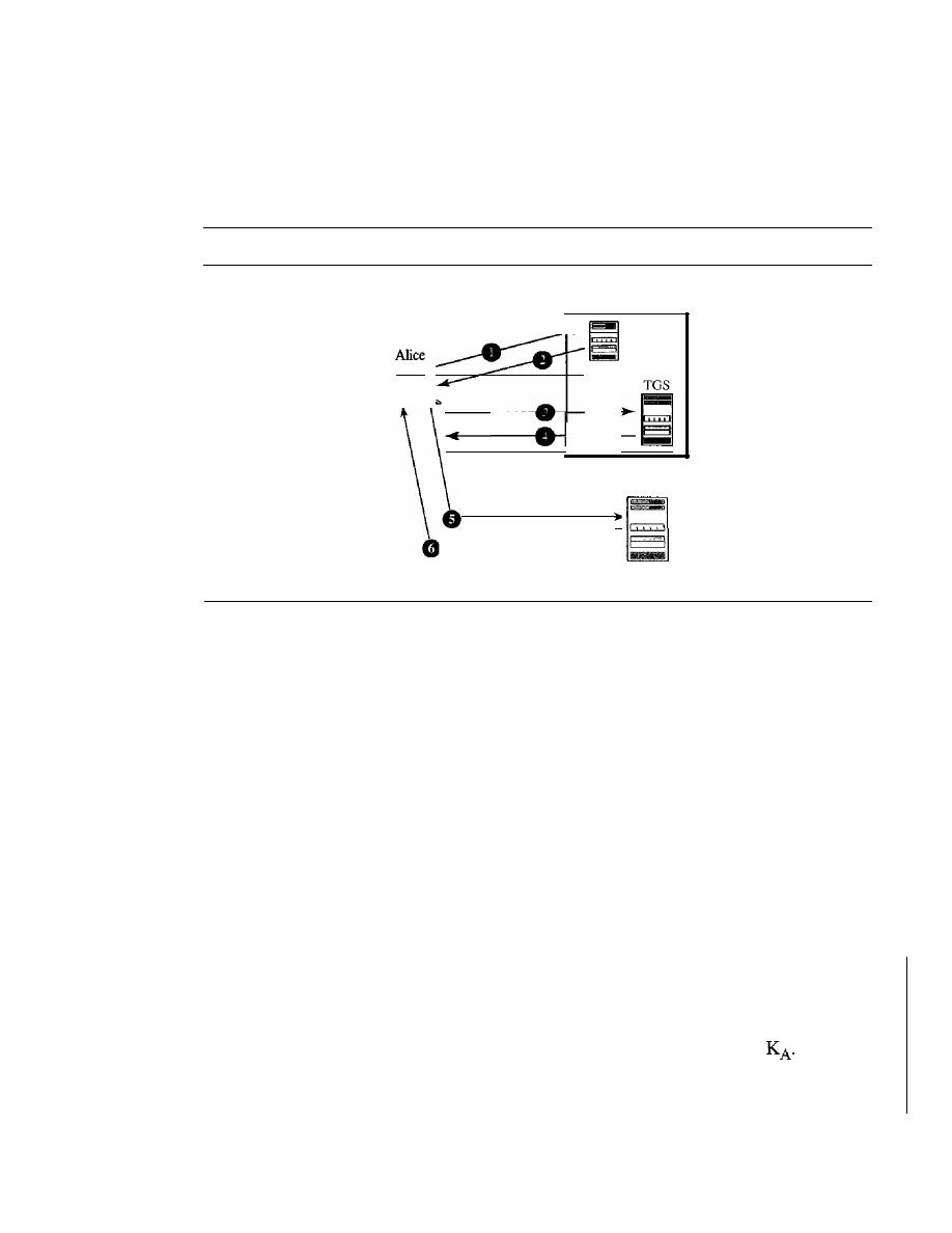
Bob (Server)
984
CHAPTER
31
NETWORK SECURITY
Servers
Three servers are involved in the Kerberos protocol: an authentication server
(AS), a ticket-granting server (TGS), and a real (data) server that provides services to
others. In our examples and figures Bob is the real server and Alice is the user request-
ing service. Figure 31.21 shows the relationship between these three servers.
Figure 31.21
Kerberos servers
1. Request ticket for TGS
2. Alice-TGS session key
and ticket for TGS
AS
3. Request ticket for Bob
4. Alice-Bob session key
_ _an_d_tl_'c_ke_t_fo_r_Bo_b
5. Request access
6. Grant access
o
Authentication Server (AS). AS is the KDC in Kerberos protocol. Each user reg-
isters with AS and is granted a user identity and a password. AS has a database
with these identities and the corresponding passwords. AS verifies the user, issues
a session key to be used between Alice and TGS, and sends a ticket for TGS.
o
Ticket-Granting Server (TGS). TGS issues a ticket for the real server (Bob).
It
also provides the session key (K
AB )
between Alice and Bob. Kerberos has sepa-
rated the user verification from ticket issuing. In this way, although Alice verifies
her ID just once with AS, she can contact TGS multiple times to obtain tickets for
different real servers.
o
Real Server. The real server (Bob) provides services for the user (Alice). Kerberos
is designed for a client/server program such as FTP, in which a user uses the client
process to access the server process. Kerberos is not used for person-to-person
authentication.
Operation
A client process (Alice) can access a process running on the real server
(Bob) in six steps as shown in Figure 31.22.
o
Step
1.
Alice sends her request to AS in plaintext, using her registered identity.
o
Step 2. AS sends a message encrypted with Alice's symmetric key
The mes-
sage contains two items: a session key K
s
that is used by Alice to contact TGS and a
ticket for TGS that is encrypted with the TGS symmetric key K
TG.
Alice does not
know K
A ,
but when the message arrives, she types her symmetric password. The
password and the appropriate algorithm together create K
A
if the password is correct.
The password is then immediately destroyed; it is not sent to the network, and it does
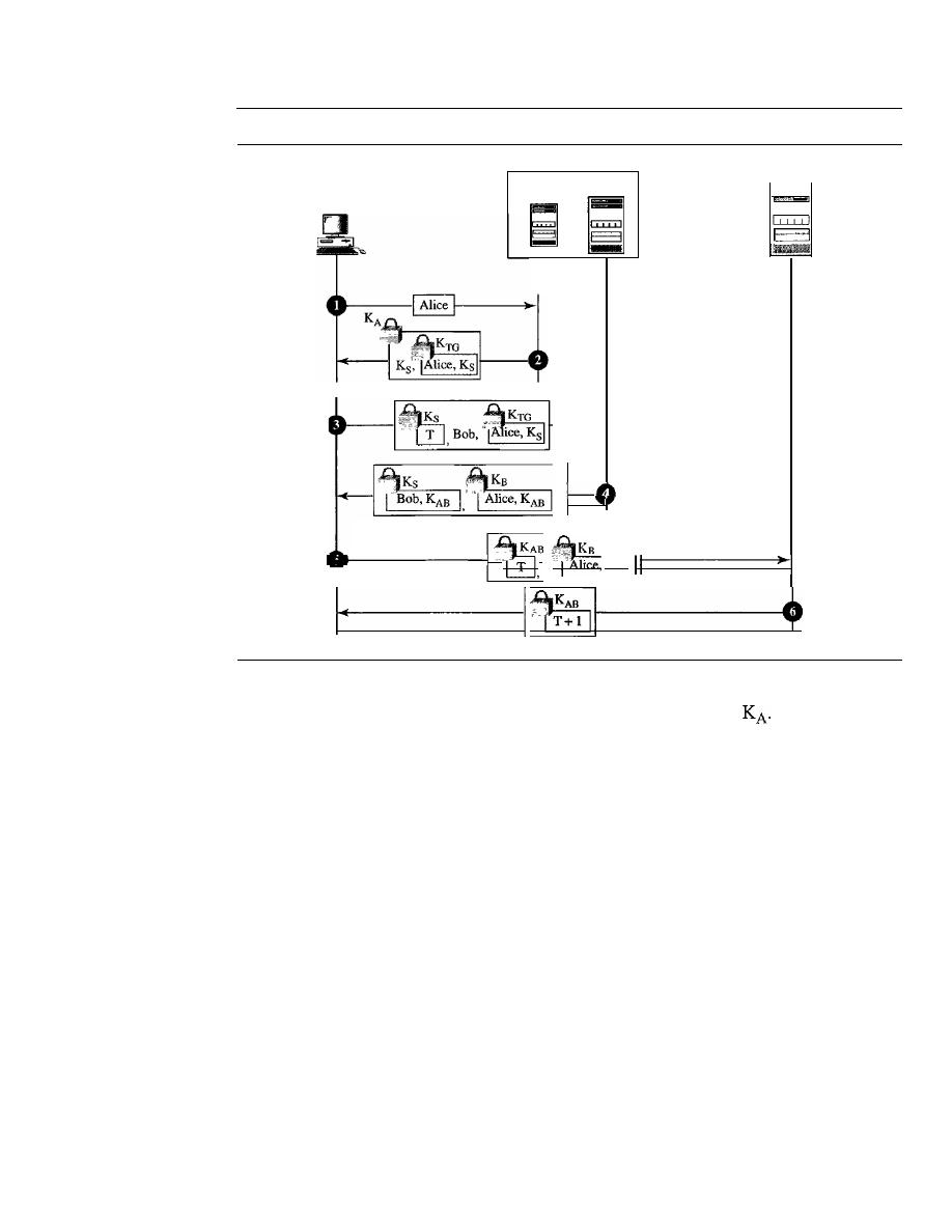
SECTION
31.7
KEY MANAGEMENT
985
Figure 31.22
Kerberos example
Server (Bob)
AS
TGS
=
Alice
I
K
AB
not stay in the terminal.
It
is only used for a moment to create
The process now
uses K
A
to decrypt the message sent. Both K
s
and the ticket are extracted.
o
Step 3. Alice now sends three items to TGS. The first is the ticket received from
AS. The second is the name of the real server (Bob), the third is a timestamp which
is encrypted by K
s.
The timestamp prevents a replay by Eve.
o
Step 4. Now, TGS sends two tickets, each containing the session key between
Alice and Bob K
AB .
The ticket for Alice is encrypted with Ks; the ticket for Bob is
encrypted with Bob's key K
B .
Note that Eve cannot extract K
AB
because she does
not know K
s
or K
B.
She cannot replay step 3 because she cannot replace the timestamp
with a new one (she does not know K
S)'
Even if she is very quick and sends the
step 3 message before the timestamp has expired, she still receives the same two
tickets that she cannot decipher.
o
Step 5. Alice sends Bob's ticket with the timestamp encrypted by K
AB .
o
Step 6. Bob confirms the receipt by adding 1 to the timestamp. The message is
encrypted with K
AB
and sent to Alice.
Using Different Servers
Note that if Alice needs to receive services from different
servers, she need repeat only steps 3 to 6. The first two steps have verified Alice's iden-
tity and need not be repeated. Alice can ask TGS to issue tickets for multiple servers by
repeating steps 3 to 6.
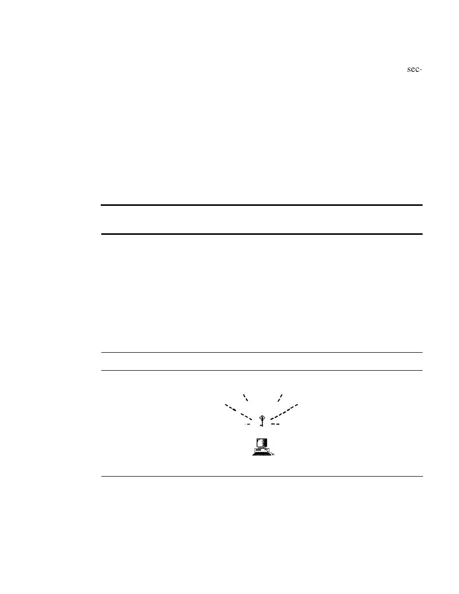
986
CHAPTER
31
NETWORK SECURITY
Realms
Kerberos allows the global distribution of ASs and TGSs, with each system
called a realm. A user may get a ticket for a local server or a remote server. In the
ond case, for example, Alice may ask her local TGS to issue a ticket that is accepted by
a remote TGS. The local TGS can issue this ticket if the remote TGS is registered with
the local one. Then Alice can use the remote TGS to access the remote real server.
Public-Key Distribution
In asymmetric-key cryptography, people do not need to know a symmetric shared key.
If
Alice wants to send a message to Bob, she only needs to know Bob's public key,
which is open to the public and available to everyone.
If
Bob needs to send a message
to Alice, he only needs to know Alice's public key, which is also known to everyone. In
public-key cryptography, everyone shields a private key and advertises a public key.
In
public-key cryptography, everyone has access to everyone's public key;
public keys are available to the public.
Public keys, like secret keys, need to be distributed to be useful. Let us briefly dis-
cuss the way public keys can be distributed.
Public Announcement
The naive approach is to announce public keys publicly. Bob can put his public key on
his website or announce it in a local or national newspaper. When Alice needs to send a
confidential message to Bob, she can obtain Bob's public key from his site or from the
newspaper, or she can even send a message to ask for it. Figure 31.23 shows the situation.
Figure 31.23
Announcing a public key
I
I
\
I
I
I
',:,'
\
I
I
\
I
------
-----
Public key
Bob
This approach, however, is not secure; it is subject to forgery. For example, Eve
could make such a public announcement. Before Bob can react, damage could be done.
Eve can fool Alice into sending her a message that is intended for Bob. Eve could also
sign a document with a corresponding forged private key and make everyone believe it
was signed by Bob. The approach is also vulnerable if Alice directly requests Bob's
public key. Eve can intercept Bob's response and substitute her own forged public key
for Bob's public key.
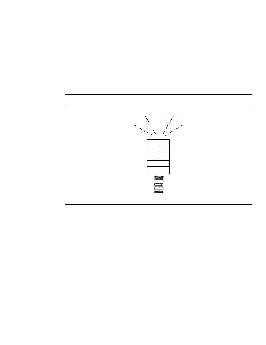
SECTION
31.7
KEY MANAGEMENT
987
Trusted Center
A more secure approach is to have a trusted center retain a directory of public keys. The
directory, like the one used in a telephone system, is dynamically updated. Each user
can select a private/public key, keep the private key, and deliver the public key for inser-
tion into the directory. The center requires that each user register in the center and
prove his or her identity. The directory can be publicly advertised by the trusted center.
The center can also respond to any inquiry about a public key. Figure 31.24 shows the
concept.
Figure 31.24
Trusted center
\
\
\
Directory
· ·
· ·
Alice
K
A
· ·
·
·
·
·
Bob
K
B
· ·
· ·
· ·
Trusted center
Controlled Trusted Center
A higher level of security can be achieved if there are added controls on the distribution
of the public key. The public-key announcements can include a timestamp and be
signed by an authority to prevent interception and modification of the response. If Alice
needs to know Bob's public key, she can send a request to the center including Bob's
name and a timestamp. The center responds with Bob's public key, the original request,
and the timestamp signed with the private key of the center. Alice uses the public key of
the center, known by
all,
to decrypt the message and extract Bob's public key. Figure 31.25
shows one scenario.
Certification Authority
The previous approach can create a heavy load on the center if the number of requests
is large. The alternative is to create public-key certificates. Bob wants two things: he
wants people to know his public key, and he wants no one to accept a public key forged
as his. Bob can go to a
certification authority
(CA)-a federal or state organization
that binds a public key to an entity and issues a certificate. The CA has a well-known
public key itself that cannot be forged. The CA checks Bob's
identification
(using a
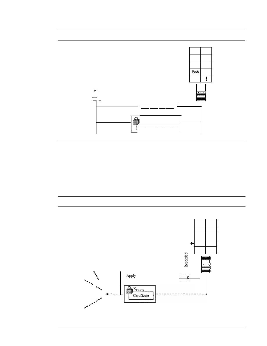
988
CHAPTER
31
NETWORK SECURITY
Figure 31.25
Controlled trusted center
Directory
· ·
·
·
· ·
Alice
KA
· ·
·
·
·
·
Kg
···
Alice
-
Trusted center
Need Bob's key, Time
KCenter
Need
Bob's
key,
Time, K
B
picture ID along with other proof). It then asks for Bob's public key and writes it on the
certificate. To prevent the certificate itself from being forged, the CA signs the certificate
with its private key. Now Bob can upload the signed certificate. Anyone who wants
Bob's public key downloads the signed certificate and uses the public key of the center
to extract Bob's public key. Figure 31.26 shows the concept.
Figure 31.26
Certification authority
Directory
__
B_I- _
Trusted
center
Issue
· ·
·
:
·
Alice
K
A
· ·
·
·
· ·
Bob
Kg
· ·
·
:
·
Bob
I
I
I
I
I
I
"
I
I
I
I
I
I
I
I
Announce to pUblic
I
I
I
I
I
' , I
\
I
,
I
--------
-

SECTION
31.7
KEY MANAGEMENT
989
X.509
Although the use of a CA has solved the problem of public-key fraud, it has
created a side effect. Each certificate may have a different format.
If
Alice
to use
a program to automatically download different certificates and digests belonging to dif-
ferent people, the program may not be able to do so. One certificate may have the public
key in one format and another in another format. The public key may be on the first line
in one certificate and on the third line in another. Anything that needs to be used univer-
sally must have a universal format.
To remove this side effect, lTD has designed a protocol called X.509, which has been
accepted by the Internet with some changes. X.509 is a way to describe the certificate in a
structured way.
It
uses a well-known protocol called ASN.1 (Abstract Syntax Notation 1)
that defines fields familiar to C programmers. The following lists the fields in a certificate.
D
Version
This field defines the version of X.509 of the certificate. The version
number started at 0; the current version is 2 (the third version).
o
Serial number
This field defines a number assigned to each certificate. The value
is unique for each certificate issued.
o
Signature
This field, for which the name is inappropriate, identifies the algorithm
used to sign the certificate. Any parameter that is needed for the signature is also
defined in this field.
o
Issuer
This field identifies the certification authority that issued the certificate. The
name is normally a hierarchy of strings that defines a country, state, organization,
department, and so on.
o
Period of validity
This field defines the earliest and the latest times the certificate
is valid.
o
Subject
This field defines the entity to which the public key belongs.
It
is also a
hierarchy of strings. Part of the field defines what is called the
common name,
which is the actual name of the beholder of the key.
o
Subject's public key
This field defines the subject's public key, the heart of the
certificate. The field also defines the corresponding algorithm (RSA, for example)
and its parameters.
o
Issuer unique identifier
This optional field allows two issuers to have the same
issuer field value, if the issuer unique identifiers are different.
D
Subject unique identifier
This optional field allows two different subjects to have
the same
subject field value, if the subject unique identifiers are different.
o
Extension
This field allows issuers to add more private information to the certificate.
o
Encrypted
This field contains the algorithm identifier, a secure hash of the other
fields, and a digital signature of that hash.
Public-Key Infrastructures (PKI)
When we want to use public keys universally, we have a problem similar to secret-key
distribution. We found that we cannot have only one KDC to answer the queries. We
need many servers. In addition, we found that the best solution is to put the servers in a
hierarchical relationship with one another. Likewise, a solution to public-key queries is
a hierarchical structure called a
public-key infrastructure (PKI).
Figure 31.27 shows
an example of this hierarchy.
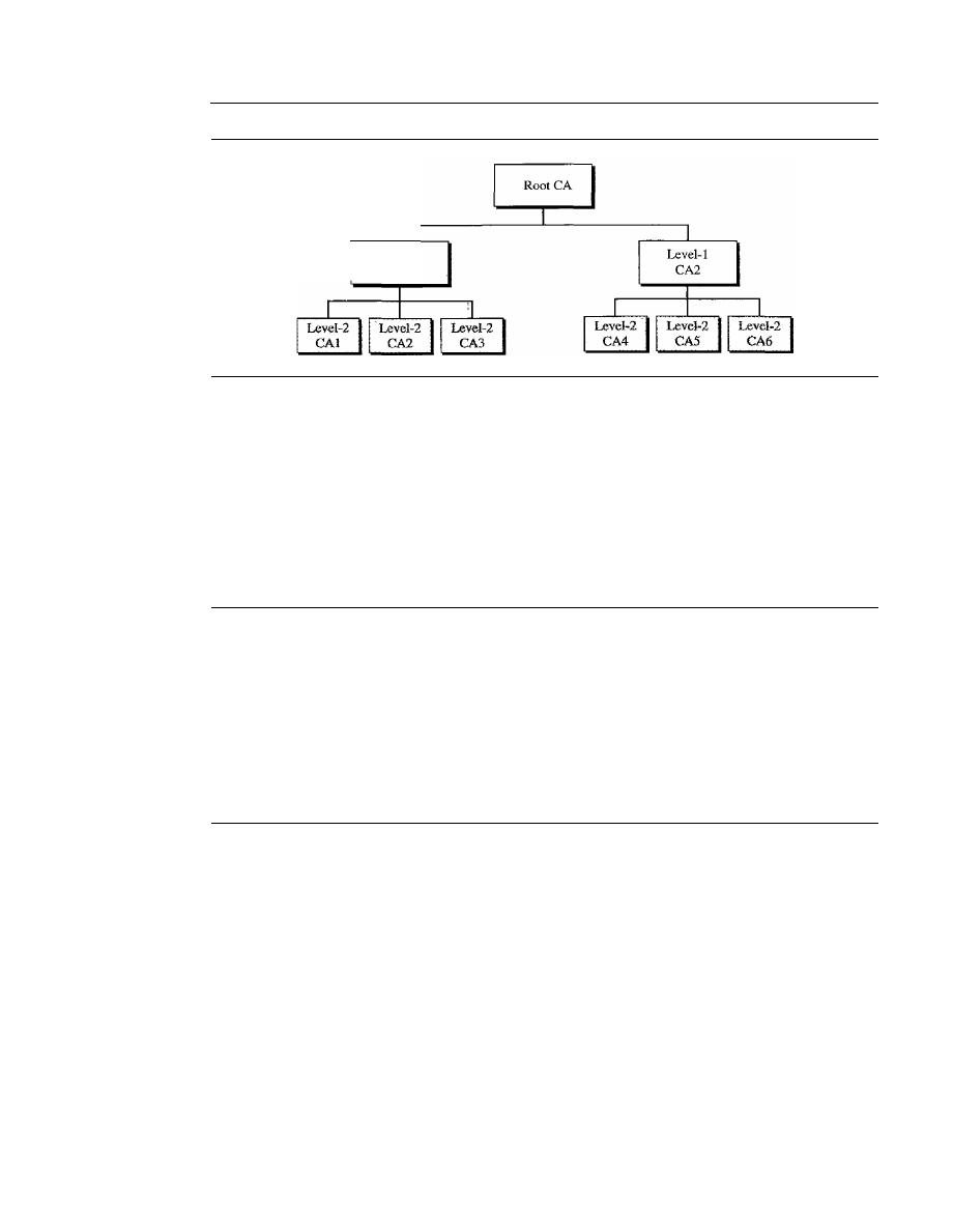
990
CHAPTER
31
NETWORK SECURITY
Figure 31.27
PKI hierarchy
Level-l
CAl
At the first level, we can have a root CA that can certify the performance of CAs in
the second level; these level-l CAs may operate in a large geographic or logical area.
The level-2 CAs may operate in smaller geographic areas.
In this hierarchy, everybody trusts the root. But people mayor may not trust inter-
mediate CAs.
If
Alice needs to get Bob's certificate, she may find a CA somewhere to
issue the certificate. But Alice may not trust that CA. In a hierarchy Alice can ask the
next-higher CA to certify the original CA. The inquiry may go all the way to the root.
31.8
RECOMMENDED READING
For more details about the subjects discussed
in
this chapter, we recommend the following
books and sites. The items in brackets [...] refer to the reference list at the end of the text.
Books
Several books are dedicated to network security, such as [PHS02], [Bis03], and [SalO3].
31.9
KEY TERMS
authentication server (AS)
certification authority (CA)
challenge-response authentication
claimant
dictionary attack
digital signature
eavesdropping
entity authentication
fingerprint
fixed password
hash function
hashed message authentication code
(HMAC)
identification
integrity
Kerberos
key distribution center (KDC)
message authentication
message authentication code (MAC)
message confidentiality or privacy
message digest
message integrity

message nonrepudiation
modification detection code
(MDC)
nonce
nonrepudiation
one-time password
one-wayness
password
privacy
public-key infrastructure
(PKI)
salting
SECTION 31.10
SUMMARY
991
session key
SHA-I
signature scheme
signing algorithm
strong collision
ticket
ticket-granting server
(TGS)
verifier
verifying algorithm
weak collision
X.509
31.10
SUMMARY
D
Cryptography can provide five services. Four of these are related to the message
exchange between Alice and Bob. The fifth is related to the entity trying to access a
system for using its resources.
D
Message confidentiality means that the sender and the receiver expect privacy.
D
Message integrity means that the data must arrive at the receiver exactly as sent.
D
Message authentication means that the receiver is ensured that the message is coming
from the intended sender, not an imposter.
D
Nonrepudiation means that a sender must not be able to deny sending a message
that he sent.
D
Entity authentication means to prove the identity of the entity that tries to access
the system's resources.
D
A message digest can be used to preserve the integrity of a document or a message.
A hash function creates a message digest out of a message.
D
A hash function must meet three criteria: one-wayness, resistance to weak collision,
and resistance to strong collision.
D
A keyless message digest is used as a modification detection code (MDC).
It
guar-
antees the integrity of the message. To authenticate the data origin, one needs a
message authentication code (MAC).
D
MACs are keyed hash functions that create a compressed digest from the message
added with the key. The method has the same basis as encryption algorithms.
D
A digital signature scheme can provide the same services provided by a conven-
tional signature. A conventional signature is included in the document; a digital
signature is a separate entity.
D
Digital signature provides message integrity, authentication, and nonrepudiation.
Digital signature cannot provide confidentiality for the message.
If
confidentiality
is needed, a cryptosystem must be applied over the scheme.

992
CHAPTER
31
NETWORK SECURiTY
o
A digital signature needs an asymmetric-key system.
o
In entity authentication, a claimant proves her identity to the verifier by using one
of the three kinds of witnesses: something known, something possessed, or some-
thing inherent.
o
In password-based authentication, the claimant uses a string of characters as some-
thing she knows.
o
Password-based authentication can be divided into two broad categories: fixed and
one-time.
o
In Challenge-response authentication, the claimant proves that she knows a secret
without actually sending it.
o
Challenge-response authentication can be divided into four categories: symmetric-
key ciphers, keyed-hash functions, asymmetric-key ciphers, and digital signature.
D
A key distribution center (KDC) is a trusted third party that assigns a symmetric
key to two parties.
o
KDC creates a secret key only between a member and the center. The secret key
between members needs to be created as a session key when two members con-
tact KDC.
D
Kerberos is a popular session key creator protocol that requires an authentication
server and a ticket-granting server.
D
A certification authority (CA) is a federal or state organization that binds a public
key to an entity and issues a certificate.
D
A public-key infrastructure (PKI) is a hierarchical system to answer queries about
key certification.
31.11
PRACTICE SET
Review Questions
1. What is a nonce?
2. What is the
N
2
problem?
3. Name a protocol that uses a KDC for user authentication.
4. What is the purpose of the Kerberos authentication server?
5. What is the purpose of the Kerberos ticket-granting server?
6. What is the purpose of X,S09?
7. What is a certification authority?
8. What are some advantages and disadvantages of using long passwords?
9. We discussed fixed and one-time passwords as two extremes. What about frequently
changed passwords? How do you think this scheme can be implemented? What are
the advantages and disadvantages?
10. How can a system prevent a guessing attack on a password? How can a bank
prevent PIN guessing if someone has found or stolen a bank card and tried to
use it?

SECTION
31.11
PRACTICE SET
993
Exercises
11. A message is made of 10 numbers between 00 and 99. A hash algorithm creates a
digest out of this message by adding all numbers modulo 100. The resulting digest
is a number between 00 and 99. Does this algorithm meet the first criterion of a
hash algorithm? Does it meet the second criterion? Does it meet the third criterion?
12. A message is made of 100 characters. A hash algorithm creates a digest out of this
message by choosing characters 1, 11,21, ..., and 91. The resulting digest has
10 characters. Does this algorithm meet the first criterion of a hash algorithm?
Does it meet the second criterion? Does it meet the third criterion?
13. A hash algorithm creates a digest of
N
bits. How many different digests can be
created from this algorithm?
14. At a party, which is more probable, a person with a birthday on a particular day or
two (or more) persons having the same birthday?
15. How is the solution to Exercise 14 related to the second and third criteria of a hashing
function?
16. Which one is more feasible, a fixed-size digest or a variable-size digest? Explain
your answer.
17. A message is 20,000 characters. We are using a digest of this message using SHA-l.
After creating the digest, we decided to change the last 10 characters. Can we say
how many bits in the digest will be changed?
18. Are the processes of creating a MAC and of signing a hash the same? What are the
differences?
19. When a person uses a money machine to get cash, is this a message authentication,
an entity authentication, or both?
20. Change Figure 31.14 to provide two-way authentication (Alice for Bob and Bob
for Alice).
21. Change Figure 31.16 to provide two-way authentication (Alice for Bob and Bob
for Alice).
22. Change Figure 31.17 to provide two-way authentication (Alice for Bob and Bob
for Alice).
23. Change Figure 31.18 to provide two-way authentication (Alice for Bob and Bob
for Alice).
24. In a university, a student needs to encrypt her password (with a unique symmetric
key) before sending it when she logs in. Does encryption protect the university or
the student? Explain your answer.
25. In Exercise 24, does it help if the student appends a timestamp to the password before
encryption? Explain your answer.
26. In Exercise 24, does it help if a student has a list of passwords and uses a different
one each time?
27. In Figure 31.20, what happens if KDC is down?
28. In Figure 31.21, what happens if the AS is down? What happens if the TGS is down?
What happens if the main server is down?
29. In Figure 31.26, what happens if the trusted center is down?

994
CHAPTER
31
NETWORK SECURITY
30. Add a symmetric-key encryption/decryption layer to Figure 31.11 to provide privacy.
31. Add an asymmetric-key encryption/decryption layer to Figure 31.11 to provide privacy.
Research Activities
32. There is a hashing algorithm called MD5. Find the difference between this algorithm
and SHA-l.
33. There is a hashing algorithm called RIPEMD-160. Find the difference between
this algorithm and SHA-l.
34. Compare
SHA-1, and RIPEMD-160.
35. Find some infonnation about RSA digital signature.
36. Find some information about DSS digital signature.
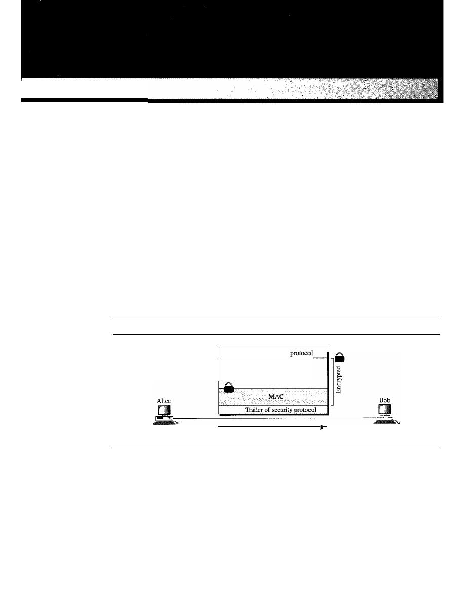
CHAPTER 32
Security in the Internet: IPSec,
SSUTLS, PGp, VPN, and Firewalls
In this chapter, we want to show how certain security aspects, particularly privacy and
message authentication, can be applied to the network, transport, and application layers of
the Internet model. We briefly show how the IPSec protocol can add authentication and
confidentiality to the IP protocol, how SSL (or TLS) can do the same for the TCP protocol,
and how PGP can do it for the SMTP protocol (e-mail).
In all these protocols, there are some common issues that we need to consider. First,
we need to create a MAC. Then we need to enCl)'pt the message and, probably, the
MAC. This means, that with some minor variations, the three protocols discussed in this
chapter take a packet from the appropriate layer and create a new packet which is authen-
ticated and encrypted. Figure 32.1 shows this general idea.
Figure 32.1
Common structure of three security protocols
Header of security
Payload
(from IP, TCP, or SMTP)
Data flow
Note that the header or the trailer of the security protocol mayor may not be included
in the encryption process. Note also that some protocols may need more information in
the secured packet; the figure shows only the general idea.
One common issue in all these protocols is security parameters. Even the simplified
structure in Figure 32.1 suggests that Alice and Bob need to know several pieces of infor-
mation, security parameters, before they can send secured data to each other. In particular,
they need to know which algorithms to use for authentication and encryption/decryption.
995

996
CHAPTER
32
SECURITY IN THE INTERNET: IPSec, SSl./TLS, PGP, VPN, AND FIREWALLS
Even if these algorithms can be predetermined for everyone in the world, which they are
not as we will see, Bob and Alice still need at least two keys: one for the MAC and one
for encryption/decryption. In other words, the complexity of these protocols lies not in
the way the MAC data are calculated or the way encryption is performed; it lies in the fact
that before calculating the MAC and performing encryption, we need to create a set of
security parameters between Alice and Bob.
At first glance, it looks as if the use of any of these protocols must involve an infi-
nite number of steps. To send secured data, we need a set of security parameters. The
secure exchange of security parameters needs a second set of security parameters. The
secure exchange of the second set of security parameters needs a third set of security
parameters. And so on ad infinitum.
To limit the steps, we can use public-key cryptography if each person has a private
and public key pair. The number of steps can be reduced to one or two. In the one-step
version, we can use session keys to create the MAC and encrypt both data and MAC.
The session keys and the list of algorithms can be sent with the packet but encrypted by
using public-key ciphers. In the two-step version, we first establish the security para-
meters by using public-key ciphers. We then use the security parameters to securely
send actual data. One of the three protocols, PGP, uses the first approach; the other two
protocols, IPSec and SSLITLS, use the second.
We also discuss a common protocol, the virtual private network (VPN), that uses
the IPSec. At the end of the chapter, we discuss the firewall, a mechanism for preventing
the attack on the network of the organization.
32.1
IPSecurity (IPSec)
IPSecurity (IPSec) is a collection of protocols designed by the Internet Engineering
Task Force (IETF) to provide security for a packet at the network level. IPSec helps to
create authenticated and confidential packets for the IP layer as shown in Figure 32.2.
Figure 32.2
TCPIIP protocol suite and IPSec
Applications
UDP, TCP, or SCTP
Two Modes
IP
Underlying physical networks
I
I
IPSec is designed
to provide security
at the network layer.
IPSec operates in one of two different modes: the transport mode or the tunnel mode as
shown in Figure 32.3.
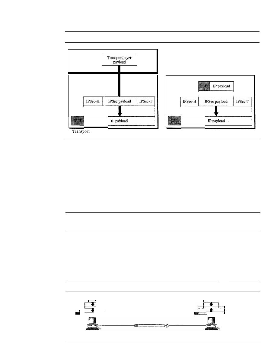
SECTION
32.1
IPSecurity (IPSec)
997
Figure 32.3
Transport mode and tunnel modes ofIPSec protocol
Transport layer
Network layer
IPSec
a.
mode
Network layer
IPSec
b. Tunnel mode
Transport Mode
In the
transport mode,
IPSec protects what is delivered from the transport layer to the
network layer. In other words, the transport mode protects the network layer payload,
the payload to be encapsulated in the network layer.
Note that the transport mode does not protect the IP header. In other words, the
transport mode does not protect the whole IP packet; it protects only the packet from
the transport layer (the IP layer payload). In this mode, the IPSec header and trailer are
added to the information corning from the transport layer. The IP header is added later.
IPSec
in
the transport mode does not protect the IP header;
it only protects the information coming from the transport layer.
The transport mode is normally used when we need host-to-host (end-to-end) pro-
tection of data. The sending host uses IPSec to authenticate and/or encrypt the payload
delivered from the transport layer. The receiving host uses IPSec to check the authenti-
cation andlor decrypt the IP packet and deliver it to the transport layer. Figure 32.4
shows this concept.
Figure 32.4
Transport mode in action
!
Transport layer
I
Transport layer
J
!
IPSec layer
IPSec layer
I Network layer
Network layer
Host A
HostB
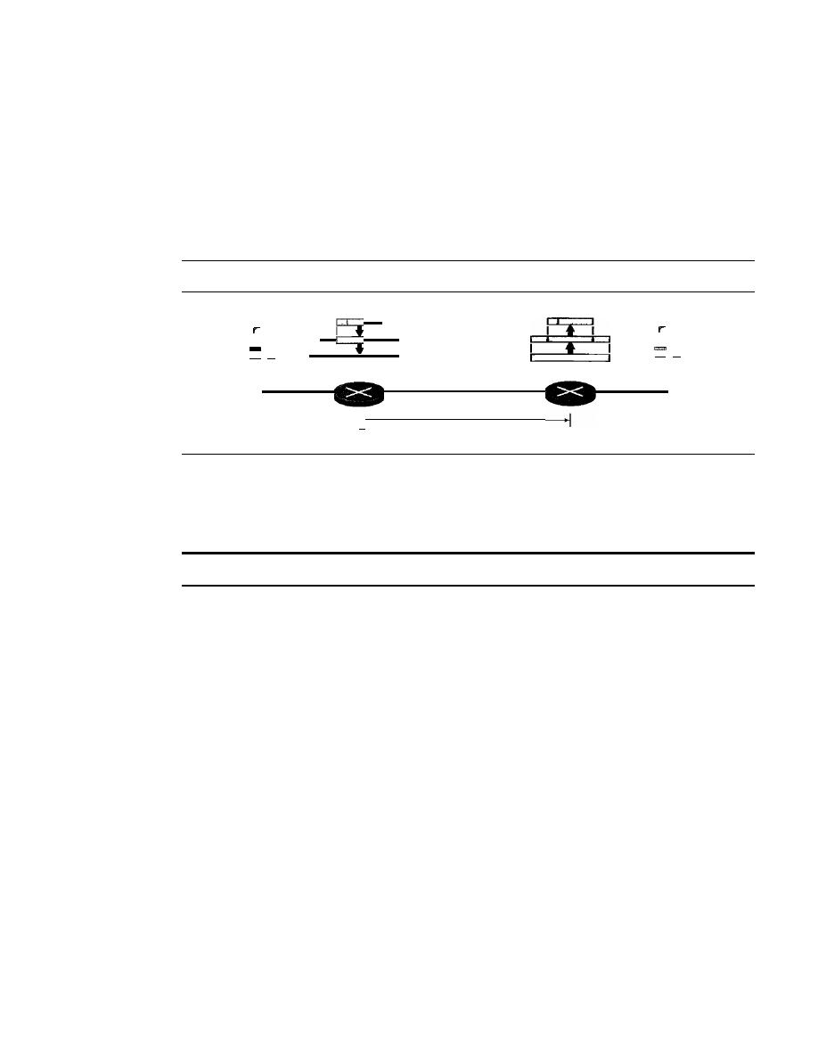
998
CHAPTER
32
SECURITY IN THE INTERNET: IPSec, SSUTLS, PGP, VPN, AND FIREWALLS
Tunnel Mode
In the
tunnel mode,
IPSec protects the entire IP packet. It takes an IP packet, including
the header, applies IPSec security methods to the entire packet, and then adds a new IP
header as shown in Figure 32.5.
The new IP header, as we will see shortly, has different information than the original
IF
header. The tunnel mode is normally used between two routers, between a host and a
router, or between a router and a host as shown in Figure 32.5.
Figure 32.5
Tunnel mode in action
Host A
-
I·
Network layer
IPSec layer
Network layer
Tunnel
Host B
-
In other words, we use the tunnel mode when either the sender or the receiver is not
a host. The entire original packet is protected from intrusion between the sender and the
receiver. It's as if the whole packet goes through an imaginary tunnel.
IPSec
in
tunnel mode protects the original IP header.
Two Security Protocols
IPSec defines two protocols-the Authentication Header (AH) Protocol and the Encap-
sulating Security Payload (ESP) Protocol-to provide authentication and/or encryption
for packets at the IP level.
Authentication Header (AH)
The
Authentication Header (AH) Protocol
is designed to authenticate the source host
and to ensure the integrity of the payload carried in the IP packet. The protocol uses a
hash function and a symmetric key to create a message digest; the digest is inserted in
the authentication header. The AH is then placed in the appropriate location based on the
mode (transport or tunnel). Figure 32.6 shows the fields and the position of the authen-
tication header in the transport mode.
When an
IP
datagram carries an authentication header, the original value in the pro-
tocol field of the IP header is replaced by the value
51.
A field inside the authentication
header (the next header field) holds the original value of the protocol field (the type of
payload being carried by the IP datagram). The addition of an authentication header
follows these steps:
1. An authentication header is added to the payload with the authentication data field
set to zero.
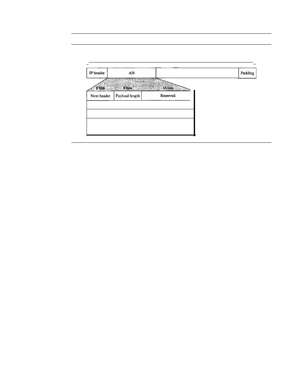
SECTION 32.1
IPSecurity (IPSec)
999
Figure 32.6
Authentication Header (AH) Protocol in transport mode
I,
Data used in calculation of authentication data
(except those fields in IP header changing during transmission)
Transport layer payload
Security parameter index
Sequence number
Authentication data (digest)
(variable length)
,I
2. Padding may be added to make the total length even for a particular hashing
algorithm.
3. Hashing is based on the total packet. However, only those fields of the IP header that
do not change during transmission are included in the calculation of the message
digest (authentication data).
4. The authentication data are inserted in the authentication header.
S.
The IP header is added after the value of the protocol field is changed to 51.
A brief description of each field follows:
o
Next header.
The 8-bit next-header field defines the type of payload carried by the
IP datagram (such as TCP, UDP, ICMP, or OSPF). It has the same function as the
protocol field in the IP header before encapsulation. In other words, the process
copies the value of the protocol field in the IP datagram to this field. The value of
the protocol field in the new IP datagram is now set to 51 to show that the packet
carries an authentication header.
o
Payload length.
The name of this 8-bit field is misleading. It does not define the
length of the payload; it defines the length of the authentication header in 4-byte
multiples, but it does not include the first 8 bytes.
o
Security parameter index.
The 32-bit security parameter index (SPI) field plays
the role of a virtual-circuit identifier and is the same for all packets sent during a
connection called a security association (discussed later).
o
Sequence number.
A 32-bit sequence number provides ordering information for
a sequence of datagrams. The sequence numbers prevent a playback. Note that the
sequence number is not repeated even if a packet is retransmitted. A sequence num-
ber does not wrap around after it reaches 2
32
;
a new connection must be established.
o
Authentication data.
Finally, the authentication data field is the result of applying
a hash function to the entire IP datagram except for the fields that are changed during
transit (e.g., time-to-live),
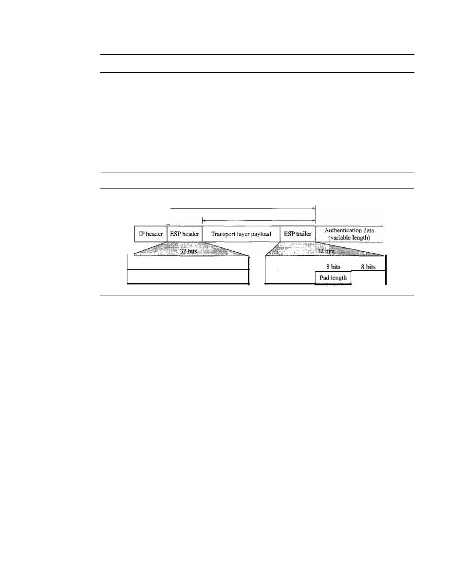
1000
CHAPTER
32
SECURITY IN THE INTERNET: IPSec, SSUFLS, PCP, VPN, AND FIREWALLS
The AH Protocol provides source authentication and data integrity, but not privacy.
Encapsulating Security Payload (ESP)
The AH Protocol does not provide privacy, only source authentication and data integrity.
IPSec later defined an alternative protocol that provides source authentication, integrity,
and privacy called
Encapsulating Security Payload (ESP).
ESP adds a header and
trailer. Note that ESP's authentication data are added at the end of the packet which
makes its calculation easier. Figure 32.7 shows the location of the ESP header and
trailer.
Figure 32.7
Encapsulation Security Payload (ESP) Protocol in transport mode
I'
Security parameter index
Sequence number
Authenticated
Encrypted
Padding
Next header
When an IP datagram carries an ESP header and trailer, the value of the protocol
field in the IP header is 50. A field inside the ESP trailer (the next-header field) holds the
original value of the protocol field (the type of payload being carried by the IP datagram,
such as TCP or UDP). The ESP procedure follows these steps:
1. An ESP trailer is added to the payload.
2. The payload and the trailer are encrypted.
3. The ESP header is added.
4. The ESP header, payload, and ESP trailer are used to create the authentication data.
5. The authentication data are added to the end of the ESP trailer.
6. The IP header is added after the protocol value is changed to 50.
The fields for the header and trailer are as follows:
o
Security parameter index.
The 32-bit security parameter index field is similar to
that defined for the AH Protocol.
o
Sequence number.
The 32-bit sequence number field is similar to that defined for
the AH Protocol.
o
Padding.
This variable-length field (0 to 255 bytes) of Os serves as padding.
o
Pad length.
The 8-bit pad length field defines the number of padding bytes. The
value is between 0 and 255; the maximum value is rare.
o
Next header.
The 8-bitnext-header field is similar to that defined in theAH Protocol.
It
serves the same purpose as the protocol field in the IP header before encapsulation.

SECTION
32.1
IPSecurity (iPSec)
1001
o
Authentication data. Finally, the authentication data field is the result of applying
an authentication scheme to parts of the datagram. Note the difference between the
authentication data in AH and ESP. In AH, part of the IP header is included in the
calculation of the authentication data; in ESP, it is not.
ESP provides source authentication, data integrity, and privacy.
IPv4 and IPv6
IPSec supports both IPv4 and IPv6. In IPv6, however, AH and ESP are part of the
extension header.
AH Versus ESP
The ESP Protocol was designed after the AH Protocol was already in use. ESP does
whatever AH does with additional functionality (privacy). The question is, Why do we
need AH? The answer is, We don't. However, the implementation of AH is already
included in some commercial products, which means that AH will remain part of the
Internet until the products are phased out.
Services Provided by IPSec
The two protocols, AH and ESP, can provide several security services for packets at the
network layer. Table 32.1 shows the list of services available for each protocol.
Table 32.1
IPSec services
Services
AH
ESP
Access control
Yes
Yes
Message authentication (message integrity)
Yes
Yes
Entity authentication (data source authentication)
Yes
Yes
Confidentiality
No
Yes
Replay attack protection
Yes
Yes
Access Control
IPSec provides access control indirectly by using a Security Associ-
ation Database (SADB) as we will see in the next section. When a packet arrives at a
destination, and there is no security association already established for this packet, the
packet is discarded.
Message Authentication
The integrity of the message is preserved in both AH and
ESP by using authentication data. A digest of data is created and sent by the sender to
be checked by the receiver.
Entity Authentication
The security association and the keyed-hashed digest of the
data sent by the sender authenticate the sender of the data in both AH and ESP.
Confidentiality
The encryption of the message in ESP provides confidentiality. AH,
however, does not provide confidentiality. If confidentiality is needed, one should use
ESP instead of AH.

1002
CHAPTER
32
SECURITY IN THE INTERNET: IPSec, SSUTLS, PGP, VPN, AND FIREWALLS
Replay Attack Protection
In both protocols, the replay attack is prevented by using
sequence numbers and a sliding receiver window. Each IPSec header contains a unique
sequence number when the security association is established. The number starts from
o
and increases until the value reaches 2
32
-
1 (the size of the sequence number field is
32 bits). When the sequence number reaches the maximum, it is reset to zero and, at the
same time, the old security association (see the next section) is deleted and a new one is
established. To prevent processing of duplicate packets, IPSec mandates the use of a
fixed-size window at the receiver. The size of the window is determined by the receiver
with a default value of 64.
Security Association
As we mentioned in the introduction to the chapter, each of three protocols we discuss
in this chapter (IPSec, SSLffLS, and PGP) needs a set of security parameters before it
can be operative. In IPSec, the establishment of the security parameters is done via a
mechanism called security association (SA).
IP, as we have seen, is a connectionless protocol: Each datagram is independent of
the others. For this type of communication, the security parameters can be established
in one of three ways.
1. Security parameters related to each datagram can be included in each datagram.
The designer of IPSec did not choose this option probably because of overhead.
Adding security parameters to each datagram creates a large overhead, particularly
if the datagram is fragmented several times during its journey.
2. A set of security parameters can be established for each datagram. This means that
before each datagram is transmitted, a set of packets needs to be exchanged between
the sender and receiver to establish security parameters. This is probably less effi-
cient than the first choice, and it is not used in IPSec.
3. IPSec uses the third choice. A set of security parameters can be established between
a sender and a particular receiver the first time the sender has a datagram to send to
that particular receiver. The set can be saved for future transmission of IP packets
to
the same receiver.
Security association is a very important aspect of IPSec. Using security association,
IPSec changes a connectionless protocol, IP, to a connection-oriented protocol. We
can think of an association as a connection. We can say that when Alice and Bob
agree upon a set of security parameters between them, they have established a logical
connection between themselves (which is called association). However, they may not
use this connection all the time. After establishing the connection, Alice can send a
datagram to Bob today, another datagram a few days later, and so on. The logical
connection is there and ready for sending a secure datagram. Of course, they can
break the connection, or they can establish a new one after a while (which is a more
secure way of communication).
A Simple Example
A security association is a very complex set of pieces of information. However, we can
show the simplest case in which Alice wants to have an association with Bob for use in
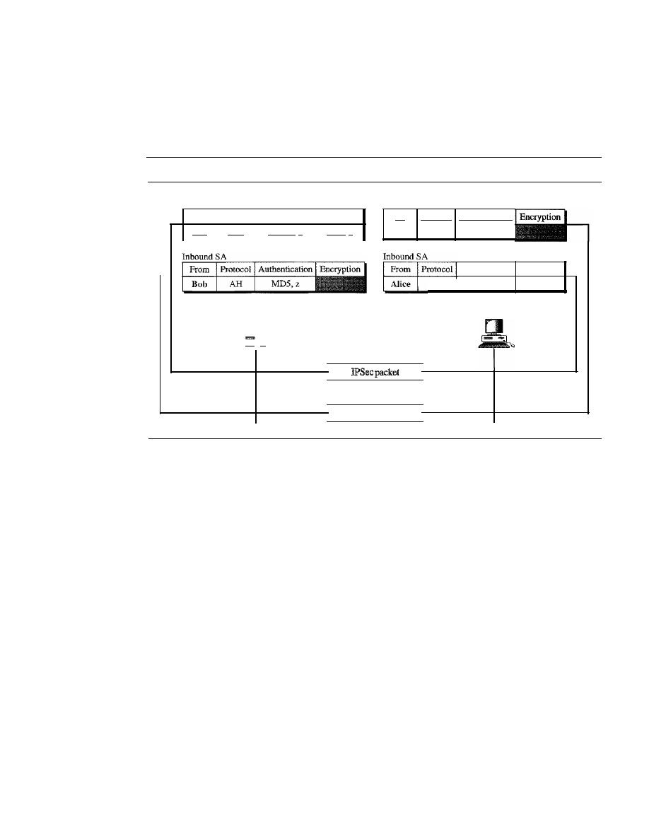
SECTION
32.1
1PSecurity (IPSec)
1003
a two-way communication. Alice can have an outbound association (for datagrams to
Bob) and an inbound association (for datagrams from Bob). Bob can have the same. In
this case, the security associations are reduced to two small tables for both Alice and
Bob as shown in Figure 32.8.
Figure 32.8
Simple inbound and outbound security associations
To
Protocol Authentication
Outbound SA
ESP
SHA-I,
x
DES, y
Outbound SA
To
Protocol Authentication Encryption
Bob
ESP
SHA-l,
x
DES, y
Alice
AH
MD5,z
Authentication Encryption
Authenticate
and encrypt
Verify
Alice
-
IPSec packet
Bob
Verify
and decrypt
Authenticate
The figure shows that when Alice needs to send a datagram to Bob, she uses the
ESP Protocol of IPSec. Authentication is done by using SHA-l with key x. The encryption
is done by using DES with key y. When Bob needs to send a datagram to Alice, he uses
the AR Protocol of IPSec. Authentication is done by using MD5 with key z. Note that
the inbound association for Bob is the same as the outbound association for Alice, and
vice versa.
Security Association Database (SADB)
A security association can be very complex. This is particularly true if Alice wants to
send messages to many people and Bob needs to receive messages from many people.
In addition, each site needs to have both inbound and outbound SAs to allow bidirectional
communication. In other words, we need a set of SAs that can be collected into a database.
This database is called the
security association database
(SADB). The database can
be thought of as a two-dimensional table with each row defining a single SA. Normally,
there are two SADBs, one inbound and one outbound.
Security Parameter Index
To distinguish one association from the other, each association is identified by a parameter
called the
security parameter index
(SPI). This parameter, in conjunction with the
destination address (outbound) or source address (inbound) and protocol (AR or ESP),
uniquely defines an association.
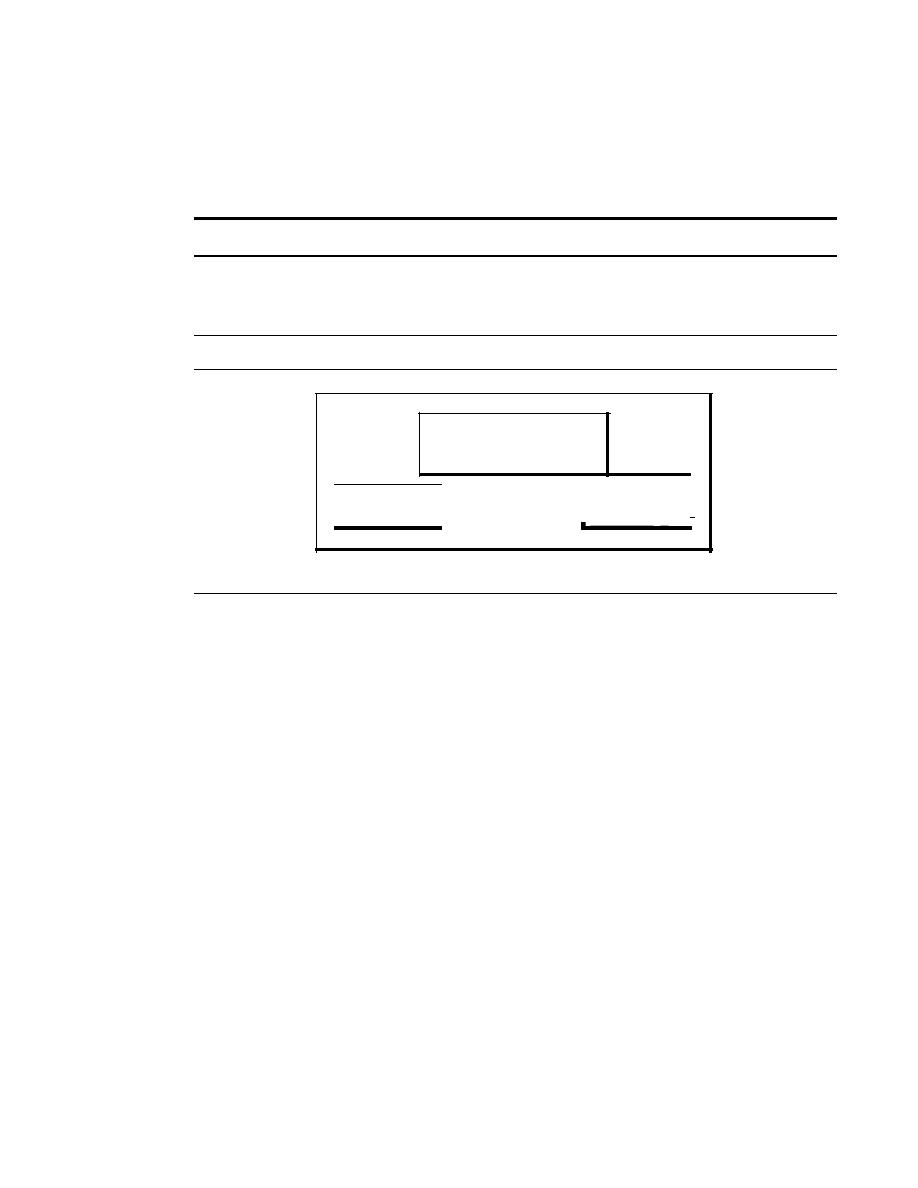
1004
CHAPTER
32
SECURITY IN THE INTERNET: IPSec, SSUTLS, PGP, VPN, AND F/REWALLS
Internet Key Exchange (IKE)
Now we come to the last part of the puzzle-how SADBs are created. The
Internet Key
Exchange (IKE)
is a protocol designed to create both inbound and outbound security
associations in SADBs.
IKE creates SAs for IPSec.
IKE is a complex protocol based on three other protocols-Oakley, SKEME, and
ISAKMP-as shown in Figure 32.9.
Figure 32.9
IKE components
Internet Security Association
and Key Management Protocol
(ISAKMP)
Oakley
SKEME
I
Internet Key Exchange (IKE)
The
Oakley
Protocol was developed by Hilarie Orman. It is a key creation protocol
based on the Diffie-Hellman key-exchange method, but with some improvements. Oakley
is a free-formatted protocol in the sense that it does not define the format of the message
to be exchanged.
SKEME,
designed by Hugo Krawcyzk, is another protocol for key exchange. It
uses public-key encryption for entity authentication in a key-exchange protocol.
The Internet Security Association and Key Management Protocol (ISAKMP)
is
a protocol designed by the National Security Agency (NSA) that actually implements the
exchanges defined in IKE.
It
defines several packets, protocols, and parameters that allow
the IKE exchanges to take place in standardized, formatted messages to create SAs.
One may ask how ISAKMP is carried from the sender to the receiver. This protocol
is designed so as to be applicable with any underlying protocol. For example, the
packet can be used as the payload in the network layer or transport layer. When we use
IPSec, it is natural that this packet be considered as a payload for the IP protocol and
carried in the datagram. Now the next question is, How are the datagrams that carry
ISAKMP securely exchanged? The answer is that there is no need. There is nothing in
the ISAKMP packets that needs to be secured.
Virtual Private Network
Virtual private network (VPN)
is a technology that is gaining popularity among large
organizations that use the global Internet for both intra- and interorganization commu-
nication, but require privacy in their internal communications. We discuss VPN here
because it uses the IPSec Protocol to apply security to the IP datagrams.

SECT/ON 32./
/PSecurity (/PSec)
1005
Private Networks
A private network is designed for use inside an organization.
It
allows access to shared
resources and, at the same time, provides privacy. Before we discuss some aspects of
these networks, let us define two commonly used, related terms:
intranet and extranet.
Intranet
An intranet is a private network (LAN) that uses the Internet model. How-
ever, access to the network is limited to the users inside the organization. The network
uses application programs defined for the global Internet, such as HTTP, and may have
Web servers, print servers, file servers, and so on.
Extranet
An extranet is the same as an intranet with one major difference: Some
resources may be accessed by specific groups of users outside the organization under
the control of the network administrator. For example, an organization may allow
authorized customers access to product specifications, availability, and online ordering.
A university or a college can allow distance learning students access to the computer
lab after passwords have been checked.
Addressing
A private network that uses the Internet model must use IP addresses.
Three choices are available:
1. The network can apply for a set of addresses from the Internet authorities and use them
without being connected to the Internet. This strategy has an advantage. If in the future
the organization decides to be connected to the Internet, it can do so with relative ease.
However, there is also a disadvantage: The address space is wasted in the meantime.
2. The network can use any set of addresses without registering with the Internet
authorities. Because the network is isolated, the addresses do not have to be unique.
However, this strategy has a serious drawback: Users might mistakenly confuse the
addresses as part of the global Internet.
3. To overcome the problems associated with the first and second strategies, the Internet
authorities have reserved three sets of addresses, shown in Table 32.2.
Table 32.2
Addresses for private networks
Prefix
Range
Total
10/8
10.0.0.0
to
10.255.255.255
2
24
172.16/12
172.16.0.0
to
172.31.255.255
2
20
192.168/16
192.168.0.0
to
192.168.255.255
2
16
Any organization can use an address out of this set without permission from the Internet
authorities. Everybody knows that these reserved addresses are for private networks.
They are unique inside the organization, but they are not unique globally. No router will
forward a packet that has one of these addresses as the destination address.
Achieving Privacy
To achieve privacy, organizations can use one of three strategies: private networks,
hybrid networks, and virtual private networks.
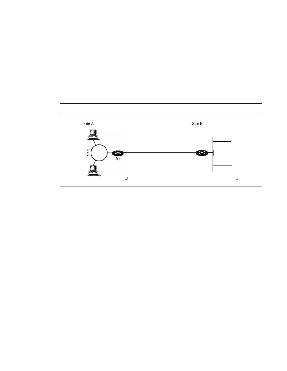
1006
CHAPTER
32
SECURITY IN THE INTERNET: IPSec, SSUTLS, PGP, VPN, AND FIREWALLS
Private Networks
An
organization that needs privacy when routing information inside
the organization can use a private network as discussed previously. A small organiza-
tion with one single site can use an isolated LAN. People inside the organization can
send data to one another that totally remain inside the organization, secure from outsiders.
A larger organization with several sites can create a private internet. The LANs at
different sites can be connected to each other by using routers and leased lines. In other
words, an internet can be made out of private LANs and private WANs. Figure 32.10
shows such a situation for an organization with two sites. The LANs are connected to
each other by routers and one leased line.
Figure 32.10
Private network
I
I
I
I
I
I
I
I
______________
Leased line
I
I
I
I
I
I
I
•
I
•
I
•
I
R2
:
I
I
I
I
I
______________
In this situation, the organization has created a private internet that is totally isolated
from the global Internet. For end-to-end communication between stations at different
sites, the organization can use the Internet model. However, there is no need for the
organization to apply for IP addresses with the Internet authorities. It can use private
IP addresses. The organization can use any IP class and assign network and host
addresses internally. Because the internet is private, duplication of addresses by another
organization in the global Internet is not a problem.
Hybrid Networks
Today, most organizations need to have privacy in intraorganization
data exchange, but, at the same time, they need to be connected to the global Internet
for data exchange with other organizations. One solution is the use of a hybrid
network. A hybrid network allows an organization to have its own private internet and,
at the same time, access to the global Internet. Intraorganization data are routed through
the private internet; interorganization data are routed through the global Internet. Fig-
ure 32.11 shows an example of this situation.
An organization with two sites uses routers Rl and R2 to connect the two sites pri-
vately through a leased line; it uses routers R3 and R4 to connect the two sites to the
rest of the world. The organization uses global IP addresses for both types of communi-
cation. However, packets destined for internal recipients are routed only through routers
Rl and R2. Routers R3 and R4 route the packets destined for outsiders.
Virtual Private Networks
Both private and hybrid networks have a major drawback:
cost. Private wide-area networks (WANs) are expensive. To connect several sites, an
organization needs several leased lines, which means a high monthly fee. One solution
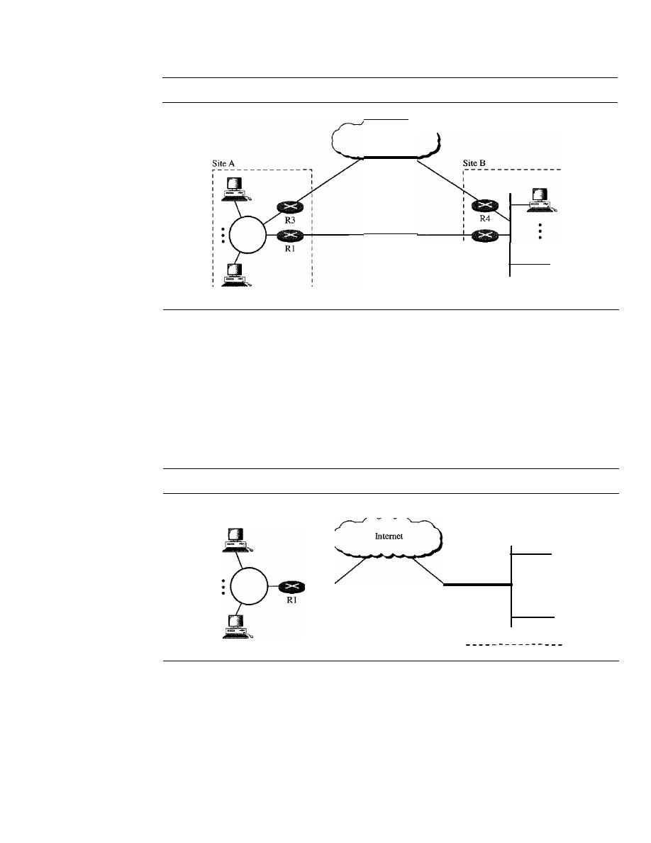
SECTION
32.1
IPSecurity (IPSe
c)
1007
Figure 32.11
Hybrid network
Internet
Leased line
R2
is to use the global Internet for both private and public communications. A technology
called virtual private network allows organizations to use the global Internet for both
purposes.
VPN creates a network that is private but virtual.
It
is private because it guarantees
privacy inside the organization.
It
is virtual because it does not use real private WANs;
the network is physically public but virtually private.
Figure 32.12 shows the idea of a virtual private network. Routers Rl and R2 use
VPN technology to guarantee privacy for the organization.
Figure 32.12
Virtual private network
R2
Site A
Site B
I
VPN Technology
VPN technology uses IPSec in the tunnel mode to provide authentication, integrity, and
privacy.
Tunneling
To guarantee privacy and other security measures for an organization,
VPN can use the IPSec in the tunnel mode. In this mode, each IP datagram destined for
private use in the organization is encapsulated in another datagram. To use IPSec in
tunneling, the VPNs need to use two sets of addressing, as shown in Figure 32.13.
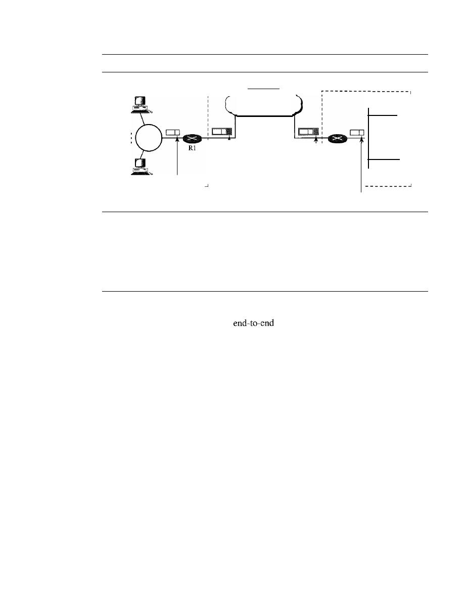
1008
CHAPTER
32
SECURITY IN THE INTERNET: IPSec, SSUTLS, PGP, VPN, AND FIREWALLS
Figure 32.13
Addressing in a VPN
r - - - - - - - - - - - - - - - - - - ,
Site A
R2
Site B
1
1
I
I
I
I
I
I
I
I
I
I
I
I
I
Station 200 :
I
I
--------
Internet
FromRl to R2
1
1
I
I
I
I
I
I
I
_ _ _ _ _
Station 100
1
- - - - - -
From 100 to 200
From 100 to 200
The public network (Internet) is responsible for carrying the packet from Rl to R2.
Outsiders cannot decipher the contents of the packet or the source and destination
addresses. Deciphering takes place at R2, which finds the destination address of the
packet and delivers it.
32.2
SSL/TLS
A transport layer security provides
security services for applications that use
a reliable transport layer protocol such as TCP. The idea is to provide security services
for transactions on the Internet. For example, when a customer shops online, the follow-
ing security services are desired:
1.
The customer needs to be sure that the server belongs to the actual vendor, not an
imposter. The customer does not want to give an imposter her credit card number
(entity authentication). Likewise, the vendor needs to authenticate the customer.
2. The customer and the vendor need to be sure that the contents of the message are
not modified during transition (message integrity).
3. The customer and the vendor need to be sure that an imposter does not intercept
sensitive information such as a credit card number (confidentiality).
Two protocols are dominant today for providing security at the transport layer: the Secure
Sockets Layer (SSL) Protocol and the Transport Layer Security (TLS) Protocol. The
latter is actually an IETF version of the former. First we discuss SSL, then we briefly
mention the main differences between SSL and TLS. Figure 32.14 shows the position
of SSL and TLS in the Internet model.
SSL Services
Secure Socket Layer (SSL) is designed to provide security and compression services
to data generated from the application layer. Typically, SSL can receive data from any
application layer protocol, but usually the protocol is HTTP. The data received from the
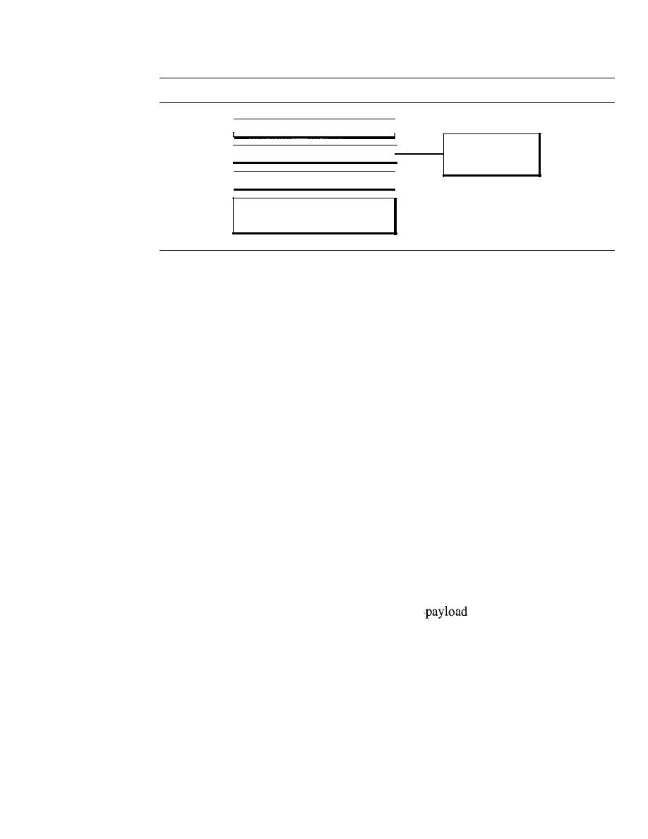
SECTION 32.2
SSUTLS
1009
Figure 32.14
Location of SSL and TLS in the Internet model
I
Applications
I
TCP
IP
Underlying physical networks
I
I
SSLrrLS is designed
to provide security
at the transport layer.
application are compressed (optional), signed, and encrypted. The data are then passed
to a reliable transport layer protocol such as TCP. Netscape developed SSL in 1994.
Versions 2 and 3 were released in 1995. In this chapter, we discuss SSLv3. SSL provides
several services on data received from the application layer.
Fragmentation
First, SSL divides the data into blocks of 2
14
bytes or less.
Compression
Each fragment of data is compressed by using one of the lossless compression methods
negotiated between the client and server. This service is optional.
Message Integrity
To preserve the integrity of data, SSL uses a keyed-hash function to create a MAC.
Confidentiality
To provide confidentiality, the original data and the MAC are encrypted using symmetric-
key cryptography.
Framing
A header is added to the encrypted payload. The
is then passed to a reliable
transport layer protocol.
Security Parameters
When we discussed IPSec in the previous section, we mentioned that each of the two
parties involved in data exchange needs to have a set of parameters for each association
(SA). SSL has a similar goal, but a different approach. There are no SAs, but there are
cipher suites and cryptographic secrets that together make the security parameters.
Cipher Suite
The combination of key exchange, hash, and encryption algorithms defines a cipher suite
for each SSL session. Each suite starts with the term SSL, followed by the key-exchange

1010
CHAPTER
32
SECURITY IN THE INTERNET: IPSec, SSUILS, PGP, VPN, AND FIREWALLS
algorithm. The word
WITH
separates the key exchange algorithm from the encryption
and hash algorithms. For example,
defines DHE_RSA (ephemeral Diffie-Hellman with RSA digital signature) as the key
exchange with DES_CBC as the encryption algorithm and SHA as the hash algorithm.
Note that DH is fixed Diffie-Hellman, DHE is ephemeral Diffie-Hellman, and DH-anon is
anonymous Diffie-Hellman. Table 32.3 shows the suites used in the United States. We
have not included those that are used for export. Note that not all combinations of key-
exchange algorithms (to establish keys for message authentication and encryption),
encryption algorithms, and authentication algorithms are included in the cipher suite list.
We have not defined or discussed several algorithms you can find in the table, but we wish
to describe the whole picture so that the reader can have an idea of how general the suite is.
Table
32.3
SSL cipher suite list
Key
Exchange
Encryption
Hash
Cipher Suite
Algorithm
Algorithm
Algorithm
SSL_NULL_WITH_NULL_NULL
NULL
NULL
NULL
SSL_RSA_WITH_NULL_MD5
RSA
NULL
MD5
SSL_RSA_WITH_NULL_SHA
RSA
NULL
SHA
SSL_RSA_WITH_RC4_128_MD5
RSA
RCU28
MD5
SSL_RSA_WITH_RC4_128_SHA
RSA
-
128
SHA
SSL_RSA_WITH_IDEA_CBC_SHA
RSA
IDEA_CSC
SHA
SSL_RSA_WITH_DES_CBC_SHA
RSA
DES_eSC
SHA
SSL_RSA_WITH_3DES_EDE_CBC_SHA
RSA
3DES_EDE_CBC
SHA
SSL_DH3ll0ll_WITH_RC4_128_MD5
DH_anon
MD5
SSL_DH_anon_WITH_DES_ CRC_SHA
DH_anon
DES_CBC
SHA
SSL_DH_anon_WITH_3DES_EDE_CBC_SHA
DH_anon
3DES_EDE_CBC
SHA
SSL_DHE_RSA_WITH_DES_CBC_SHA
DHE_RSA
DES_CBC
SHA
SSL_DHE_RSA_WITH_3DES_EDE_CBC_SHA
DHE_RSA
SHA
SSL_DHE_DSS_WITH_DES_CBCSHA
DHE_DSS
SHA
SSL_DHE_DSS_WITH_3DES_EDE_CBC_SHA
DHE_DSS
DBS_EDE_CSC
SHA
SSL_DH_RSA_WITH_DES_CRC_SHA
DH_RSA
DES_CBC
SHA
SSL_DH_RSA_WITH_3DES_EDE_CBC_SHA
DH_RSA
30BS_EDE_CSC
SHA
SSL_DH_DSS_ WITH_DES_CBC_SHA
DH_DSS
DES_CEC
SHA
SSL_DH_DSS_ WITH_3DES_EDE_CBC_SHA
DH_DSS
SHA
SSL_FORTEZZA_DMS_WITH_NULL_SHA
FORTEZZA_DMS
NULL
SHA
SSL_FORTEZZA_DMS_WITH_FORTEZZA_CRC_SHA
FORTEZZA_DMS
FORTEZZA_CBC
SHA
SSL]ORTEZZA_DMS_WITH_RC4_128_SHA
FORTEZZA_DMS
SHA
Cryptographic Secrets
The second part of security parameters is often referred to as cryptographic secrets. To
achieve message integrity and confidentiality, SSL needs six cryptographic secrets, four
keys, and two IVs.
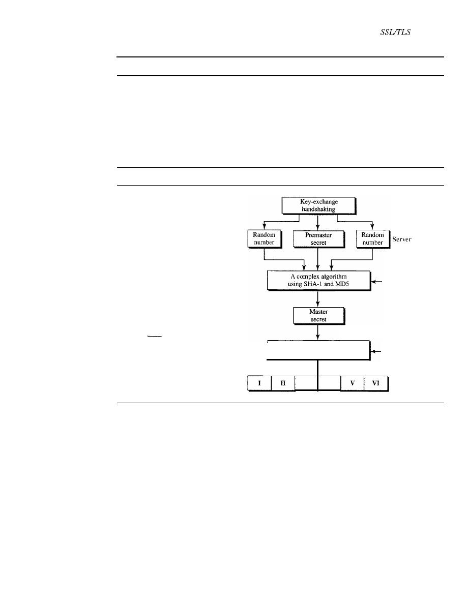
SECTION
32.2
1011
The client and the server have six different cryptography secrets.
The process of creating these secrets is shown in Figure 32.15. The client needs
one key for message authentication, one key for encryption, and one IV for block
encryption. The server needs the same. SSL requires that the keys for one direction be
different from those for the other direction.
If
there is an attack in one direction, the
other direction is not affected. These parameters are generated by using a negotiation
protocol, as we will see shortly.
Figure
32.15
Creation of cryptographic secrets in SSL
Client
I
- - Client authentication key
II - -
Server authentication key
III - -
Client encryption key
IV - - Server encryption key
V
- -
Client initiation vector
VI
Server initiation vector
A complex algorithm
using SHA-I and MD5
Some constants
Some constants
III
IV
1. The client and server exchange two random numbers; one is created by the client
and the other by the server.
2. The client and server exchange one premaster secret by using one of the key-
exchange algorithms we discussed previously.
3. A 48-byte master secret is created from the premaster secret by applying two hash
functions (SHA-l and MD5).
4. The master secret is used
to
create variable-length secrets by applying the same set
of hash functions and prepending with different constants.
Sessions and Connections
The nature of IP and TCP protocols is different. IP is a connectionless protocol; TCP is
a connection-oriented protocol. An association in IPSec transforms the connectionless
IP to a connection-oriented secured protocol. TCP is already connection-oriented.
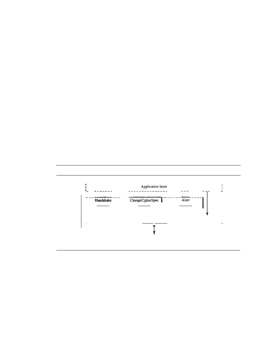
1012
CHAPTER
32
SECURITY IN THE INTERNET: IPSec, SSurLS, PGP, VPN, AND FIREWALLS
However, the designers of SSL decided that they needed two-levels of connectivity:
session and connection. A session between two systems is an association that can last for
a long time; a connection can be established and broken several times during a session.
Some of the security parameters are created during the session establishment and
are in effect until the session is terminated (for example, cipher suite and master key).
Some of the security parameters must be recreated (or occasionally resumed) for each
connection (for example, six secrets).
Four Protocols
We have discussed the idea of SSL without showing how SSL accomplishes its tasks.
SSL defines four protocols in two layers, as shown in Figure 32.16. The Record Protocol
is the carrier. It carries messages from three other protocols as well as the data coming
from the application layer. Messages from the Record Protocol are payloads to the
transport layer, normally TCP. The Handshake Protocol provides security parameters
for the Record Protocol.
It
establishes a cipher set and provides keys and security
parameters.
It
also authenticates the server to the client and the client to the server, if
needed. The ChangeCipherSpec Protocol is used for signaling the readiness of cryp-
tographic secrets. The Alert Protocol is used to report abnormal conditions. We will
briefly discuss these protocols in this section.
Figure 32.16
Four SSL protocols
SSL
,---------------------------------------------------1
--
------
----- -----
----
Protocol
Protocol
Protocol
I
Record Protocol
I
,
1
:
Transport layer
:
I
J
Handshake Protocol
The Handshake Protocol uses messages to negotiate the cipher suite, to authenticate the
server to the client and the client to the server (if needed), and to exchange information
for building the cryptographic secrets. The handshaking is done in four phases, as shown
in Figure 32.17.
ChangeCipherSpec Protocol
We have seen that the negotiation of the cipher suite and the generation of crypto-
graphic secrets are formed gradually during the Handshake Protocol. The question now
is, When can the two parties use these parameter secrets? SSL mandates that the parties
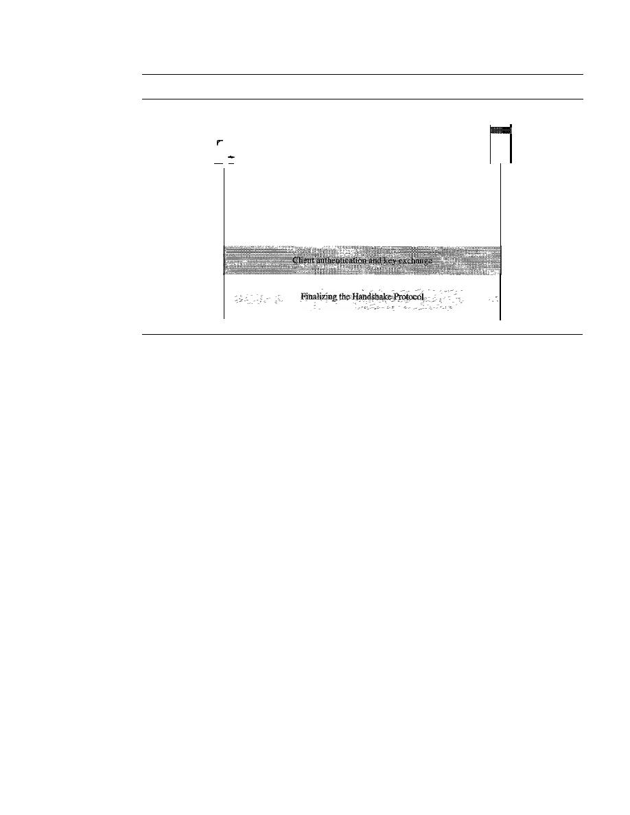
SECTION
32.2
SSUFLS
1013
Figure 32.17
Handshake Protocol
Client
-
Phase I
Establishing Security Capabilities
Server authentication and key exchange
Server
Phase II
Phase III
Phase IV
not use these parameters or secrets until they have sent or received a special message,
the ChangeCipherSpec message, which is exchanged during the Handshake Protocol and
defined in the ChangeCipherSpec Protocol. Before the exchange of any ChangeCipherSpec
messages, only the pending columns have values.
Alert Protocol
SSL uses the Alert Protocol for reporting errors and abnormal conditions.
It
has only one
message type, the alert message, that describes the problem and its level (warning or fatal).
Record Protocol
The Record Protocol carries messages from the upper layer (Handshake Protocol,
ChangeCipherSpec Protocol, Alert Protocol, or application layer). The message is frag-
mented and optionally compressed; a MAC is added to the compressed message by
using the negotiated hash algorithm. The compressed fragment and the MAC are
encrypted by using the negotiated encryption algorithm. Finally, the SSL header is
added to the encrypted message. Figure 32.18 shows this process at the sender. The
process at the receiver is reversed.
Transport Layer Security
Transport Layer Security (TLS) is the IETF standard version of SSL. The two are
very similar, with slight differences. We highlight the differences below:
o
Version. The SSLv3.0 discussed in this section is compatible with TLSv1.0.
o
Cipher Suite. TLS cipher suite does not support Fortezza.
o
Cryptography Secret. There are several differences in the generation of crypto-
graphic secrets. TLS uses a
pseudorandom function (PRF) to create the master
key and the key materials.
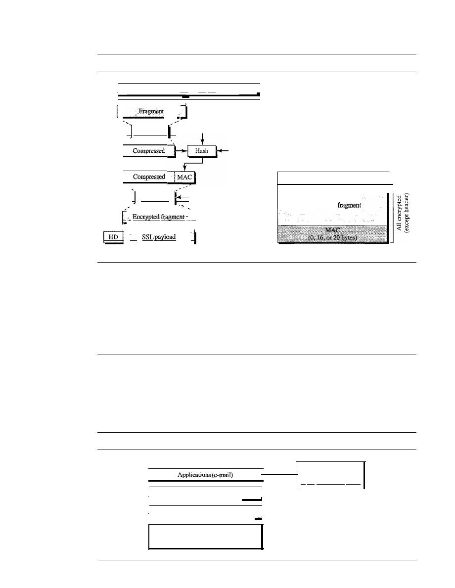
1014
CHAPTER
32
SECURITY IN THE INTERNET: IPSec, SSUTLS, PGP, VPN, AND FIREWALLS
Figure 32.18
Processing done
by
the Record Protocol
SSLHeader
Authentication key
Constant
Compression
I
Payload from upper-layer protocol
:
I
Encryption
Encryption key
)
a. Process
b. Packet
Compressed
o
Alert Protocol. TLS deletes some alert messages and adds some new ones.
o
Handshake Protocol. The details of some messages have been changed in TLS.
o
Record Protocol. Instead of using MAC, TLS uses the HMAC as defined in
Chapter 31.
32.3
PGP
One of the protocols to provide security at the application layer is Pretty Good Privacy
(PGP). PGP is designed to create authenticated and confidential e-mails. Figure 32.19
shows the position of PGP in the TCP/IP protocol suite.
Figure 32.19
Position of PGP in the TCPlIP protocol suite
I
UDP, TCP. or SCTP
_ _ _ _ _
I
I
I
PGP is designed
to provide security
at the application layer.
I
IP
Underlying physical networks

SECTION
32.3
PGP
1015
Sending an e-mail is a one-time activity. The nature of this activity is different
from those we have seen in the previous two sections. In IPSec or SSL, we assume that
the two parties create a session between themselves and exchange data in both direc-
tions. In e-mail,there is no session. Alice and Bob cannot create a session. Alice sends
a message to Bob; sometime later, Bob reads the message and mayor may not send a
reply. We discuss the security of a unidirectional message because what Alice sends to
Bob is totally independent of what Bob sends to Alice.
Security Parameters
If e-mail is a one-time activity, how can the sender and receiver agree on the security
parameters to use for e-mail security? If there is no session and no handshaking to
negotiate the algorithms for encryption and authentication, how can the receiver know
which algorithm the sender has chosen for each purpose? How can the receiver know
the values of the keys used for encryption and authentication?
Phil Zimmerman, the designer and creator of PGP, has found a very elegant solution
to the above questions. The security parameters need to be sent with the message.
In PGP, the sender of the message needs to include the identifiers of the
algorithms used in the message as well as the values of the keys.
Services
PGP can provide several services based on the requirements of the user. An e-mail can
use one or more of these services.
Plaintext
The simplest case is to send the e-mail message in plaintext (no service). Alice, the
sender, composes a message and sends it to Bob, the receiver. The message is stored in
Bob's mailbox until it is retrieved by him.
Message Authentication
Probably the next improvement is to let Alice sign the message. Alice creates a digest
of the message and signs it with her private key. When Bob receives the message, he
verifies the message by using Alice's public key. Two keys are needed for this scenario.
Alice needs to know her private key; Bob needs to know Alice's public key.
Compression
A further improvement is to compress the message and digest to make the packet more
compact. This improvement has no security benefit, but it eases the traffic.
Confidentiality with
Time Session Key
As we discussed before, confidentiality in an e-mail system can be achieved by using
conventional encryption with a one-time session key. Alice can create a session key, use
the session key to encrypt the message and the digest, and send the key itself with the
message. However, to protect the session key, Alice encrypts it with Bob's public key.
1016
CHAPTER
32
SECURITY IN THE INTERNET: IPSec,
PGP, VPN, AND FIREWALLS
Code Conversion
Another service provided by PGP is code conversion. Most
systems allow the
message to consist of only ASCII characters. To translate other characters not in the
ASCII set, PGP uses Radix 64 conversion. Each character to be sent (after encryption)
is converted to Radix 64 code.
Segmentation
PGP allows segmentation of the message after it has been converted to Radix 64 to
make each
unit the uniform size allowed by the underlying
protocoL
A Scenario
Let us describe a scenario that combines some of these services, authentication and
confidentiality. The whole idea of PGP is based on the assumption that a group of people
who need to exchange
messages trust one another. Everyone in the group
how knows (with a degree of trust) the public key of any other person in the group.
Based on this single assumption, Figure 32.20 shows a simple scenario in which an
authenticated and encrypted message is sent from Alice to Bob.
Figure 32.20
A scenario in which an e-mail message is authenticated and encrypted
Alice's Bob's
private public
Alice
-
Bob's Alice's
private public
Bob
PGPmessage
PGP
header
PAl
+
PAl: Public-key algorithm 1 (for encrypting session key)
PA2: PubliC-key algorithm (for encrypting the digest)
SA: Symmetric-key algorithm identification (for encrypting message and digest)
HA: Hash algorithm identification (for creating digest)
Sender Site
The following shows the steps used in this scenario at Alice's site:
1. Alice creates a session key (for symmetric encryption/decryption) and concatenates
it with the identity of the algorithm which will use this key. The result is encrypted

SECTION
32.3
PGP
1017
with Bob's public key. Alice adds the identification of the public-key algorithm
used above to the encrypted result. This part of the message contains three pieces
of information: the session key, the symmetric encryption/decryption algorithm to
be used later, and the asymmetric encryption/decryption algorithm that was used
for this part.
2.
a. Alice authenticates the message (e-mail) by using a public-key signature algo-
rithm and encrypts it with her private key. The result is called the signature.
Alice appends the identification of the public key (used for encryption) as well
as the identification of the hash algorithm (used for authentication) to the signa-
ture. This part of the message contains the signature and two extra pieces of
information: the encryption algorithm and the hash algorithm.
b. Alice concatenates the three pieces of information created above with the message
(e-mail) and encrypts the whole thing, using the session key created in step 1.
3. Alice combines the results of steps 1 and 2 and sends them to Bob (after adding tue
appropriate PGP header).
Receiver Site
The following shows the steps used in this scenario at Bob's side after he has received
the PGP packet:
1.
Bob uses his private key to decrypt the combination of the session key and
symmetric-key algorithm identification.
2. Bob uses the session key and the algorithm obtained in step 1 to decrypt the rest of
the PGP message. Bob now has the content of the message, the identification of the
public algorithm used for creating and encrypting the signature, and the identifica-
tion of the hash algorithm used to create the hash out of the message.
3. Bob uses Alice's public key and the algorithm defined by PA2 to decrypt the digest.
4. Bob uses the hash algorithm defined by HA to create a hash out of message he
obtained in step 2.
5. Bob compares the hash created in step 4 and the hash he decrypted in step 3.
If
the
two are identical, he accepts the message; otherwise, he discards the message.
PGP Algorithms
Table 32.4 shows some of the algorithms used in POP. The list is not complete; new
algorithms are continuously added.
Table 32.4
Algorithm
ID
Description
Public key
1
RSA (encryption or signing)
2
RSA (for encryption only)
3
RSA (for signing only)
17
DSS
(for signing)
1018
CHAPTER
32
SECURITY IN THE INTERNET: IPSec, SSLfTLS, PGP, VPN, AND FIREWALLS
Table 32.4
(continued)
Algorithm
ID
Description
Hash algorithm
1
MD5
2
SHA-l
3
RIPE-MD
Encryption
0
No encryption
1
IDEA
2
Triple DES
9
AES
Key
Rings
In the previous scenarios, we assumed that Alice needed to send a message to only Bob.
That is not always the case. Alice may need to send messages to many people. In this
case, Alice needs a key
ring
of public keys, with a key belonging to each person with
whom Alice needs to correspond (send or receive messages). In addition, the PGP
designers specified a ring of private/public keys. One reason is that Alice may wish to
change her pair of keys from time to time. Another reason is that Alice may need to
correspond with different groups of people (friends, colleagues, and so on). Alice may
wish to use a different key pair for each group. Therefore, each user needs to have
two sets of rings: a ring of private/public keys and a ring of public keys of other people.
Figure 32.21 shows a community of four people, each having a ring of pairs of private/
public keys and, at the same time, a ring of four public keys belonging to the other four
people in the community. The figure shows seven public keys for each public ring. Each
person in the ring can keep more than one public key for each other person.
Figure 32.21
Rings
Alice's rings
Bob's rings
John's rings

SECTION
32.3
PGP
1019
Alice, for example, has several pairs of private/public keys belonging to her and
public keys belonging to other people. Note that everyone can have more than one public
key. Two cases may arise.
1. Alice needs to send a message to one of the persons in the community.
a. She uses her private key to sign the digest.
b. She uses the receiver's public key to encrypt a newly created session key.
c. She encrypts the message and signs the digest with the session key created.
2. Alice receives a message from one of the persons in the community.
a. She uses her private key to decrypt the session key.
b. She uses the session key to decrypt the message and digest.
c. She uses her public key to verify the digest.
PGP Certificates
To trust the owner of the public key, each user in the PGP group needs to have, implicitly
or explicitly, a copy of the certificate of the public-key owner. Although the certificate
can come from a certificate authority (CA), this restriction is not required in PGP. PGP
has its own certificate system.
Protocols that use X509 certificates depend on the hierarchical structure of the
trust. There is a predefined chain of trust from the root to any certificate. Every user
fully trusts the authority of the CA at the root level (prerequisite). The root issues certif-
icates for the CAs at the second level, a second-level CA issues a certificate for the
third level, and so on. Every party that needs to be trusted presents a certificate from
some CA in the tree.
If
Alice does not trust the certificate issuer for Bob, she can appeal
to a higher-level authority up to the root (which must be trusted for the system to work).
In other words, there is one single path from a fully trusted CA to a certificate.
In PGP, there is no need for CAs; anyone in the ring can sign a certificate for any-
one else in the ring. Bob can sign a certificate for Ted, John, Anne, and so on. There is
no hierarchy of trust in PGP; there is no tree. As a result of the lack of hierarchical
structure, Ted may have one certificate from Bob and another certificate from Liz.
If
Alice wants to follow the line of certificates for Ted, it has two paths: one starts from
Bob and the other starts from Liz. An interesting point is that Alice may fully trust Bob,
but only partially trust Liz. There can be multiple paths in the line of trust from a fully
or partially trusted authority to a certificate. In PGP, the issuer of a certificate is usually
called an introducer.
In PGP, there can be multiple paths from runy or
partially trusted authorities to any subject.
Trusts and Legitimacy
The entire operation of PGP is based on introducer trust, the certificate trust, and the
legitimacy of the public keys.
Introducer Trust Levels
With the lack of a central authority, it is obvious that the ring
cannot be very large if every user in the PGP ring of users has to fully trust everyone else.

1020
CHAPTER
32
SECURITY IN THE INTERNET: IPSec, SSUFLS, PGP, VPN, AND FIREWALLS
(Even in real life we cannot fully trust everyone that we know.) To solve this problem,
PGP allows different levels of trust. The number of levels is mostly implementation-
dependent, but for simplicity, let us assign three levels of trust to any introducer:
none,
partial,
and
full.
The introducer trust level specifies the trust levels issued by the intro-
ducer for other people in the ring. For example, Alice may fully trust Bob, partially trust
Anne, and not trust John at alL There is no mechanism in PGP to determine how to make
a decision about the trustworthiness of the introducer; it is up to the user to make this
decision.
Certificate Trust Levels
When Alice receives a certificate from an introducer, she
stores the certificate under the name of the subject (certified entity). She assigns a level
of trust to this certificate. The certificate trust level is normally the same as the intro-
ducer trust level that issued the certificate. Assume Alice fully trusts Bob, partially
trusts Anne and Janette, and has no trust in John. The following scenarios can happen.
1. Bob issues two certificates, one for Linda (with public key K1) and one for Lesley
(with public key K2). Alice stores the public key and certificate for Linda under
Linda's name and assigns a
full
level of trust to this certificate. Alice also stores the
certificate and public key for Lesley under Lesley's name and assigns a full level of
trust to this certificate.
2. Anne issues a certificate for John (with public key K3). Alice stores this certificate
and public key under John's name, but assigns a
partial
level for this certificate.
3. Janette issues two certificates, one for John (with public key K3) and one for Lee
(with public key K4). Alice stores John's certificate under his name and Lee's cer-
tificate under his name, each with a
partial
level of trust. Note that John now has
two certificates, one from Anne and one from Janette, each with a
partial
level
of trust.
4. John issues a certificate for Liz. Alice can discard or keep this certificate with a
signature trust of
none.
Key Legitimacy
The purpose of using introducer and certificate trusts is to deter-
mine the legitimacy of a public key. Alice needs to know how legitimate are the public
keys of Bob, John, Liz, Anne, and so on. PGP defines a very clear procedure for deter-
mining key legitimacy. The level of the key legitimacy for a user is the weighted trust
of that user. For example, suppose we assign the following weights to certificate
trust levels:
1. A weight of 0 to a nontrusted certificate
2. A weight of
to a certificate with partial trust
3. A weight of 1 to a certificate with full trust
Then to fully trust an entity, Alice needs one fully trusted certificate or two partially
trusted certificates for that entity. For example, Alice can use John's public key in the
previous scenario because both Anne and Janette have issued a certificate for John,
each with a certificate trust level of
!.
Note that the legitimacy of a public key belonging
2
to an entity does not have anything to do with the trust level of that person. Although
Bob can use John's public key to send a message to him, Alice cannot accept any certif-
icate issued by John because, for Alice, John has a trust level of
none.

SECTION
32.4
FIREWALLS
1021
Starting the Ring
You might have realized a problem with the above discussion. What if nobody sends a
certificate for a fully or partially trusted entity? For example, how can the legitimacy
of Bob's public key be determined if no one has sent a certificate for Bob? In PGP, the
key legitimacy of a trusted or partially trusted entity can be also determined by other
methods.
1. Alice can physically obtain Bob's public key. For example, Alice and Bob can meet
personally and exchange a public key written on a piece of paper or to a disk.
2.
If
Bob's voice is recognizable to Alice, Alice can call him and obtain his public key
on the phone.
3. A better solution proposed by PGP is for Bob to send his public key to Alice by
e-mail. Both Alice and Bob make a 16-byte MD5 (or 20-byte SHA-l) digest
from the key. The digest is normally displayed as eight groups of four digits (or
10 groups of four digits) in hexadecimal and is called a fingerprint. Alice can then
call Bob and verify the fingerprint on the phone. If the key is altered or changed
during the e-mail transmission, the two fingerprints do not match. To make it even
more convenient, PGP has created a list of words, each representing a four-digit
combination. When Alice calls Bob, Bob can pronounce the eight words (or
10 words) for Alice. The words are carefully chosen by PGP to avoid those similar
in pronunciation; for example, if
sword
is in the list,
word
is not.
4. In PGP, nothing prevents Alice from getting Bob's public key from a CA in a
rate procedure. She can then insert the public key in the public-key ring.
Web of Trust
PGP can eventually make a web of trust between a group of people.
If
each entity
introduces more entities to other entities, the public-key ring for each entity gets larger
and larger and entities in the ring can send secure e-mail to one another.
Key Revocation
It
may become necessary for an entity to revoke his or her public key from the ring.
This may happen if the owner of the key feels that the key is compromised (stolen, for
example) or just too old to be safe. To revoke a key, the owner can send a revocation
certificate signed by herself. The revocation certificate must be signed by the old key
and disseminated to all the people in the ring who use that public key.
32.4
FIREWALLS
All previous security measures cannot prevent Eve from sending a harmful message to a
system. To control access to a system, we need firewalls. A firewall is a device (usually a
router or a computer) installed between the internal network of an organization and the
rest of the Internet.
It
is designed to forward some packets and filter (not forward) others.
Figure 32.22 shows a firewall.
1022
CHAPTER
32
SECURITY IN THE INTERNET: IPSec, SSUTLS, PGP, VPN, AND FIREWALLS
Figure 32.22
Firewall
Firewall
For example, a firewall may filter all incoming packets destined for a specific host
or a specific server such as HTTP. A firewall can be used to deny access to a specific
host or a specific service in the organization.
A firewall is usually classified as a packet-filter firewall or a proxy-based firewall.
Packet-Filter Firewall
A firewall can be used as a packet filter. It can forward or block packets based on the
information in the network layer and transport layer headers: source and destination
IP addresses, source and destination port addresses, and type of protocol (TCP or UDP).
A packet-filter firewall is a router that uses a filtering table to decide which packets
must be discarded (not forwarded). Figure 32.23 shows an example of a filtering table
for this kind of a firewall.
Figure 32.23
Packet-filter firewall
Packet-filter
firewall
To and from
global Internet
Interface
Source
Source
Destination
Destination
IP
porl
IP
port
131.34.0.0
*
*
*
*
*
*
23
*
*
194.78.20.8
*
2
*
80
*
*
According to Figure 32.23, the following packets are filtered:
). Incoming packets from network 131.34.0.0 are blocked (security precaution). Note
that the
*
(asterisk) means "any."
2. Incoming packets destined for any internal TELNET server (port 23) are blocked.
3. Incoming packets destined for internal host 194.78.20.8 are blocked. The organiza-
tion wants this host for internal use only.
4. Outgoing packets destined for an HTfP server (port 80) are blocked. The organi-
zation does not want employees to browse the Internet.
SECTION
32.4
FlREWALLS
1023
A
firewall filters at the network or transport layer.
Proxy Firewall
The packet-filter firewall is based on the information available in the network layer and
transport layer headers (IP and TCPIUDP). However, sometimes we need to filter a
message based on the information available in the message itself (at the application
layer). As an example, assume that an organization wants to implement the following
policies regarding its Web pages: Only those Internet users who have previously estab-
lished business relations with the company can have access; access to other users must
be blocked. In this case, a packet-filter firewall is not feasible because it cannot distin-
guish between different packets arriving at TCP port 80 (HTTP). Testing must be done
at the application level (using URLs).
One solution is to install a proxy computer (sometimes called an application gate-
way), which stands between the customer (user client) computer and the corporation
computer shown in Figure 32.24.
Figure 32.24
Proxy firewall
Errors
HTIPproxy
Global Internet
All HTIP
packets
HTIP server
Accepted
packets
When the user client process sends a message, the proxy firewall runs a server
process to receive the request. The server opens the packet at the application level and
finds out if the request is legitimate.
If
it
is, the server acts as a client process and sends
the message to the real server in the corporation.
If
it
is not, the message is dropped and
an error message is sent to the external user. In this way, the requests of the external
users are filtered based on the contents at the application layer.. Figure 32.24 shows a
proxy firewall implementation.
A proxy firewall filters at the application layer.

1024
CHAPTER
32
SECURITY IN THE INTERNET: IPSec, SSUTLS, PGP, VPN, AND FIREWALLS
32.5
RECOMMENDED READING
For more details about subjects discussed in this chapter, we recommend the following
books. The brackets, [...], refer to the reference list at the end of the text.
Books
IPSec is discussed in Chapter 7 of [Rhe03], Section 18.1 of [PHS03], and Chapters 17
and 18 of [KPS02]. A full discussion ofIPSec can be found in [DH03]. SSLITLS is dis-
cussed in Chapter 8 of [Rhe03], and Chapter 19 of [KPS02]. A full discusion of SSL and
TLS can be found in [ResOl] and [ThoOO]. PGP is discussed in Chapter 9 of [Rhe03], and
Chapter 22 of [KPS02]. Firewalls are discussed in Chapter 10 of [Rhe03] and Chapter 23
of [KPS02]. Firewalls are fully discussed in [CBR03]. Virtual private networks are fully
discussed in [YSO 1] and [SWE99].
32.6
KEY TERMS
Alert Protocol
Authentication Header (AH)
Protocol
certificate trust
ChangeCipherSpec Protocol
cipher suite
connection
Encapsulating Security Payload
(ESP)
extranet
fingerprint
firewall
Handshake Protocol
hybrid network
Internet Key Exchange (IKE)
Internet Security Association and Key
Management Protocol (lSAKMP)
intranet
introducer
introducer trust
IP
Security (IPSec)
key legitimacy
key material
key ring
master secret
Oakley
packet-filter firewall
premaster secret
Pretty Good Privacy (PGP)
private network
proxy firewall
pseudorandom function (PRF)
Record Protocol
replay attack
Secure Socket Layer (SSL)
security association (SA)
security association database
(SADB)
security parameter index (SPI)
session
SKEME
Transport Layer Security
(TLS)
transport mode
tunnel mode
tunneling
virtual private network (VPN)
web of trust

SECTION
32. 7
SUMMARY
1025
32.7
SUMMARY
o
IP Security (IPSec) is a collection of protocols designed by the IETF (Internet
Engineering Task Force) to provide security for a packet at the network level.
o
IPSec operates in the transport mode or the tunnel mode.
o
In the transport mode, IPSec protects information delivered from the transport
layer to the network layer. IPSec in the transport mode does not protect the IP header.
The transport mode is normally used when we need host-to-host (end-to-end) pro-
tection of data.
o
In the tunnel mode, IPSec protects the whole IP packet, including the original IP
header.
o
IPSec defines two protocols-Authentication Header (AH) Protocol and Encapsu-
lating Security Payload (ESP) Protocol-to provide authentication or encryption
or both for packets at the IP level.
o
IPSec requires a logical relationship between two hosts called a security association
(SA). IPSec uses a set of SAs called the security association database or SADB.
o
The Internet Key Exchange (IKE) is the protocol designed to create security asso-
ciations, both inbound and outbound. IKE creates SAs for IPSec.
[l
IKE is a complex protocol based on three other protocols: Oakley, SKEME, and
ISAKMP.
o
A private network is used inside an organization.
o
An intranet is a private network that uses the Internet model. An extranet is an
intranet that allows authorized access from outside users.
o
The Internet authorities have reserved addresses for private networks.
[]
A virtual private network (VPN) provides privacy for LANs that must communicate
through the global Internet.
o
A transport layer security protocol provides end-to-end security services for appli-
cations that use the services of a reliable transport layer protocol such as TCP.
o
Two protocols are dominant today for providing security at the transport layer:
Secure Sockets Layer (SSL) and Transport Layer Security (TLS). The second is
actually an IETF version of the first.
o
SSL is designed to provide security and compression services to data generated
from the application layer. Typically, SSL can receive application data from any
application layer protocol, but the protocol is normally HTTP.
SSL provides services such as fragmentation, compression, message integrity,
fidentiality, and framing on data received from the application layer.
o
The combination of key exchange, hash, and encryption algorithms defines a cipher
suite for each SSL session. The name of each suite is descriptive of the combination.
In e-mail, the cryptographic algorithms and secrets are sent with the message.
D
One security protocol for the e-mail system is Pretty Good Privacy (PGP). PGP
was invented by Phil Zimmerman to provide privacy, integrity, and authentication
in e-mail.

1026
CHAPTER
32
SECURITY IN THE INTERNET: IPSec, SSUFLS, PGP, VPN, AND FIREWALLS
o
To exchange e-mail messages, a user needs a ring of public keys; one public key is
needed for each e-mail correspondent.
o
POP has also specified a ring of private/public key pairs to allow a user to change
her pair of keys from time to time. POP also allows each user to have different user
IDs (e-mail addresses) for different groups of people.
o
POP certification is different from X509. In X509, there is a single path from the
fully trusted authority to any certificate. In POP, there can be multiple paths from
fully or partially trusted authorities.
o
pap
uses the idea of certificate trust levels.
o
When a user receives a certificate from an introducer, it stores the certificate under
the name of the subject (certified entity).
It
assigns a level of trust to this certificate.
32.8
PRACTICE SET
Review Questions
1.
Why does IPSec need a security association?
2.
How does IPSec create a set of security parameters?
3.
What are the two protocols defined by IPSec?
4.
What does AH add to the IP packet?
5. What does ESP add to the IP packet?
6. Are both AH and ESP needed for IP security? Why or why not?
7.
What are the two protocols discussed in this chapter that provide security at the
transport layer?
8. What is IKE?
9. What is the difference between a session and a connection in SSL?
10. How does SSL create a set of security parameters?
11. What is the name of the protocol, discussed in this chapter, that provides security
for e-mail?
12. How does PGP create a set of security parameters?
13. What is the purpose of the Handshake Protocol in SSL?
14. What is the purpose of the Record Protocol in SSL?
15. What is the purpose of a firewall?
16. What are the two types of firewalls?
17. What is a VPN and why is it needed?
18. How do LANs on a fully private internet communicate?
Exercises
19. Show the values of the AH fields in Figure 32.6. Assume there are 128 bits of
authentication data.
20. Show the values of the ESP header and trailer fields in Figure 32.7.

SECTION
32.8
PRACTICE SET
1027
21. Redraw Figure 32.6 if AH is used in tunnel mode.
22. Redraw Figure 32.7 if ESP is used in tunnel mode.
23. Draw a figure to show the position of AH in IPv6.
24. Draw a figure to show the position of ESP in IPv6.
25. Does the IPSec Protocol need the services of a KDC? Explain your answer.
26. Does the IPSec Protocol need the services of a CA? Explain your answer.
27. Does the SSL Protocol need the services of a KDC? Explain your answer.
28. Does the SSL Protocol need the services of a CA? Explain your answer.
29. Does the PGP Protocol need the services of a KDC? Explain your answer.
30. Does the
pap
Protocol need the services of a CA? Explain your answer.
31. Are there any cipher suites in IPSec? Explain your answer.
32. Are there any cipher suites in PGP? Explain your answer.

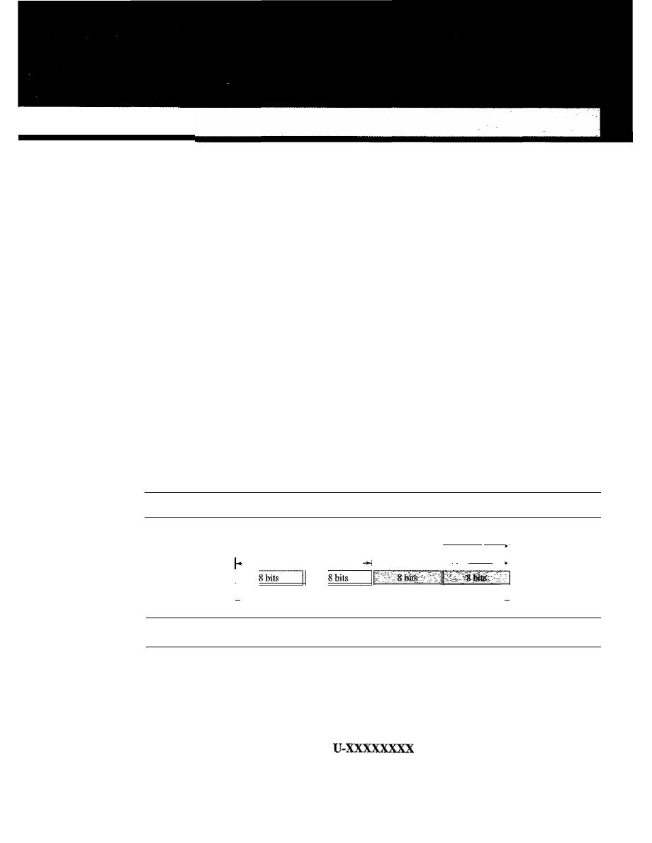
APPENDIX A
Unicode
Computers use numbers. They store characters by assigning a number for each one. The
original coding system was called ASCII (American Standard Code for Information
Interchange) and had 128 numbers (0 to 127) each stored as a 7-bit number. ASCII could
satisfactorily handle lowercase and uppercase letters, digits, punctuation characters, and
some control characters. An attempt was made to extend the ASCII character set to 8 bits.
The new code, which was called Extended ASCII, was never internationally standardized.
To overcome the difficulties inherent in ASCII and Extended ASCII, the Unicode
Consortium (a group of multilingual software manufacturers) created a universal
encoding system to provide a comprehensive character set called Unicode.
Unicode was originally a 2-byte character set. Unicode version 3, however, is a
4-byte code and is fully compatible with ASCII and Extended ASCII. The ASCII set,
which is now called Basic Latin, is Unicode with the upper 25 bits set to zero. Extended
ASCII, which is now called Latin-I, is Unicode with the 24 upper bits set to zero. Fig-
ure A.I shows how the different systems are compatible.
Figure A.l
Unicode compatibility
"
Extended ASCII
I
•
D_e_fin_in_g_p_lan_e_s_ _
I
1•
ASCII
1__
_ _
I,
Unicode
.j
A.I
UNICODE
The prevalent code today is Unicode. Each character or symbol in this code is defined
by a 32-bit number. The code can define up to 2
32
(4,294,967,296) characters or sym-
bols. The notation uses hexadecimal digits in the following format:
1029
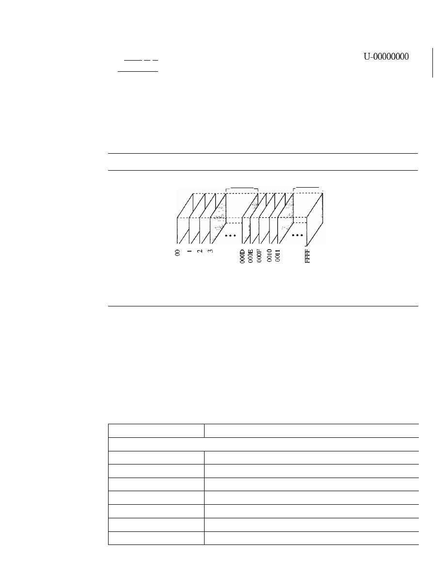
1030
APPENDIX A
UNICODE
Each X is a hexadecimal digit. Therefore, the numbering goes from
to
U-FFFFFFFF.
Planes
Unicode divides the available space codes into planes. The most significant 16 bits
define the plane, which means we can have 65,535 planes. Each plane can define up to
65,536 character or symbols. Figure A.2 shows the structure of Unicode spaces and
planes.
Figure A.2
Unicode planes
a
a
a
a
a
a
a
a
a
a
a
Reserved
Reserved
Plane 0000: Basic Multilingual Plane (BMP)
Plane 0001: Supplementary Multilingual Plane (SMP)
Plane 0002: Supplementary Ideographic Plane (SIP)
Plane OOOE: Supplementary Special Plane (SSP)
Plane OOOF: Private Use Plane (PUP)
Plane 0010: Private Use Plane (PUP)
Basic Multilingual Plane (BMP)
Plane 0000, the basic multilingual plane (BMP), is designed to be compatible with the
previous 16-bit Unicode. The most significant 16 bits in this plane are all zeros. The codes
are normally shown as U+XXXX with the understanding that XXXX defines only the
least significant 16 bits. This plane mostly defines character sets in different languages
with the exception of some codes used for control or other special characters. Table A.I
shows the main classification of codes in plane 0000.
Table A.I
Unicode BMP
Range
Description
,
A-Zone (Alphabetical Characters and Symbols)
U+OOOO to U+OOFF
Basic Latin and Latin-l
U+OIOO to U+OIFF
Latin extended
U+0200 to U+02FF
IPA extension, and space modifier letters
U+0300 to U+03FF
Combining diacritical marks, Greek
U+0400 to U+04FF
Cyrillic
U+0500 to U+05FF
Armenian, Hebrew
U+0600 to U+06FF
Arabic

Table A.I
Unicode BMP (continued)
APPENDIX A
UNICODE
1031
Range
Description
U+0700 to U+08FF
Reserved
U+0900 to U+09FF
Devanagari, Bengali
U+OAOO to U+OAFF
Gumukhi, Gujarati
U+OBOO to U+OBFF
Oriya, Tamil
U+OCOO to U+OCFF
Telugu, Kannda
U+ODOO to U+ODFF
Malayalam
U+OEOO to U+OEFF
Thai, Lao
U+OFOO to U+OFFF
Reserved
U+ 1000 to U+ lOFF
Georgian
U+1100 to U+llFF
Hangul Jamo
U+1200 to U+1DFF
Reserved
U+IEOO to U+1EFF
Latin extended additional
U+1FOO to U+1FFF
Greek extended
U+2000 to U+20FF
Punctuation, sub/superscripts, currency, marks
U+21 00 to U+21FF
Letterlike symbols, number forms, arrows
U+2200 to U+22FF
Mathematical operations
U+2300 to U+23FF
Miscellaneous technical symbols
U+2400 to U+24FF
Control pictures, OCR, and enclosed alphanumeric
U+2500 to U+25FF
Box drawing, block drawing, and geometric shapes
U+2600 to U+26FF
Miscellaneous symbols
U+2700 to U+27FF
Dingbats and Braille patterns
U+2800 to U+2FFF
Reserved
U+3000 to U+30FF
CJK symbols and punctuation, hiragana, katakana
U+3100 to U+31FF
Bopornfo, hangul jambo, cjk miscellaneous
U+3200 to U+32FF
Enclosed CJK letters and months
U+3300 to U+33FF
CJK compatibility
U+3400 to U+4DFF
Hangul
I-Zone (Ideographic Characters)
U+4EOO to U+9FFF
CJK unified ideographic
O-Zone (Open)
U+AOOO to U+DFFF
Reserved
R·Zone (Restricted Use)
U+EOOO to U+F8FF
Private use
U+F900 to U+FAFF
CJK compatibility ideographs
U+FBOO to U+FBFF
Arabic presentation form-A

1032
APPENDIX A
UNICODE
Table A.I
Unicode BMP (continued)
Range
Description
I
I
U+FCOO to U+FDFF
Arabic presentation form-B
U+FEOO to U+FEFF
Half marks, small forms
U+FFOO to U+FFFF
Half-width and full-width forms
I
I
Supplementary Multilingual Plane (SMP)
Plane 0001, the supplementary multilingual plane (SMP), is designed to provide more
codes for those multilingual characters that are not included in the BMP.
Supplementary Ideographic Plane (SIP)
Plane 0002, the supplementary ideographic plane (SIP), is designed to provide codes for
ideographic symbols, symbols that primarily denote an idea (or meaning) in contrast to a
sound (or pronunciation).
Supplementary Special Plane (SSP)
Plane OOOE, the supplementary special plane (SSP), is used for special characters.
Private Use Planes (PUPs)
Planes OOOF and 0010, private use planes (PUPs), are for private use.
A.2
ASCII
The American Standard Code for Information Interchange (ASCII) is a 7-bit code that
was designed to provide code for 128 symbols, mostly in American English. Today,
ASCII, or Basic Latin, is part of Unicode.
It
occupies the first 128 codes in Unicode
(00000000 to 0000007F). Table A.2 contains the decimal, hexadecimal, and graphic
codes (symbols) with an English interpretation,
if
appropriate. The codes in hexadecimal
just define the two least significant digits in Unicode. To find the actual code, we prepend
000000 in hexadecimal to the code. The decimal code is just to show the integer value
of each symbol when converted.
Table A.2
ASCII Codes
Decimal
Hex
Symbol
Interpretation
0
00
null
Null value
1
01
SOH
Start of heading
2
02
STX
Start of text
3
03
ETX
End of text
4
04
EaT
End of transmission

Table
A.2
ASCII Codes (continued)
APPENDIX A
UN/CODE
1033
Decimal
Hex
Symbol
Interpretation
5
05
ENQ
Enquiry
6
06
ACK
Acknowledgment
7
07
BEL
Ring bell
8
08
BS
Backspace
9
09
HT
Horizontal tab
10
OA
LF
Line feed
11
OB
VT
Vertical tab
12
OC
FF
Fonn feed
13
OD
CR
Carriage return
14
OE
SO
Shift out
15
OF
SI
Shift in
16
10
DLE
Data link escape
17
11
DC1
Device control 1
18
12
DC2
Device control 2
19
13
DC3
Device control 3
20
14
DC4
Device control 4
21
15
NAK
Negative acknowledgment
22
16
SYN
Synchronous idle
23
17
ETB
End of transmission block
24
18
CAN
Cancel
25
19
EM
End of medium
26
1A
SUB
Substitute
27
lB
ESC
Escape
28
1C
FS
File separator
29
10
GS
Group separator
30
IE
RS
Record separator
31
IF
US
Unit separator
32
20
SP
Space
33
21
!
34
22
n
Double quote
35
23
#
36
24
$
37
25
%
38
26
&
39
27
,
Apostrophe

1034
APPENDIX A
UNICODE
Table
A.2
ASCII Codes (continued)
Decimal
Hex
Symbol
Interpretation
I
40
28
(
41
29
)
42
2A
*
43
2B
+
44
2C
,
Comma
45
2D
-
Minus
46
2E
47
2F
/
48
30
0
49
31
1
50
32
2
51
33
3
52
34
4
53
35
5
54
36
6
55
37
7
56
38
8
57
39
9
58
3A
Colon
59
3B
,
Semicolon
60
3C
<
61
3D
=
62
3E
>
63
3F
?
64
40
@
65
41
A
66
42
B
67
43
C
68
44
D
69
45
E
70
46
F
71
47
G
72
48
H
73
49
I
74
4A
J

Table
A.2
ASCII Codes (continued)
APPENDIX A
UNICODE
1035
Decimal
Hex
Symbol
Interpretation
75
4B
K
76
4C
L
77
4D
M
78
4E
N
79
4F
0
80
50
P
81
51
Q
_ .
'-
-
_.-
_
..
82
52
R
83
53
S
84
54
T
85
55
U
86
56
V
87
57
W
88
58
X
89
59
y
90
5A
Z
91
5B
[
Open bracket
92
5C
\
Backs1ash
93
5D
]
Close bracket
94
5E
Caret
95
5F
Underscore
96
60
Grave accent
97
61
a
98
62
b
99
63
c
100
64
d
101
65
e
102
66
f
103
67
g
104
68
h
105
69
i
106
6A
J
107
6B
k
108
6C
1
109
6D
m

1036
APPENDIX A
UNICODE
Table A.2
ASCII Codes (continued)
Decimal
Hex
Symbol
Interpretation
110
6E
n
111
6F
0
112
70
p
113
71
q
114
72
r
115
73
s
116
74
t
117
75
u
118
76
v
119
77
w
120
78
x
121
79
y
122
7A
z
123
7B
{
Open brace
124
7C
I
Bar
125
7D
}
Close brace
126
7E
Tilde
127
7F
DEL
Delete
SOllIe Properties of ASCII
ASCII has some interesting properties that we briefly mention here.
I.
The first code (0) is the null character, which means the lack of any character.
2. The first 32 codes, 0 to 31, are control characters.
The space character, which is a printable character, is at position 32.
4. The uppercase letters start from 65 (A). The lowercase letters start from 97. When
compared, uppercase letters are numerically smaller than lowercase letters. This
means that in a sorted list based on ASCII values, the uppercase letters appear
before the lowercase letters.
5. The uppercase and lowercase letters differ by only one bit in the 7-bit code. For exam-
ple, character A is 1000001 (Ox4l) and character a is 110000 I(Ox61). The difference
is in bit 6, which is 0 in uppercase letters and 1 in lowercase letters.
If
we know the
code for one case, we can easily find the code for the other by adding or subtracting
32 in decimal (Ox20 in hexadecimal), or we can just flip the sixth bit.
6. The uppercase letters are not immediately followed by lowercase letters. There are
some punctuation characters in between.
7. Digits (0 to 9) start from 48 (Ox3). This means that if you want to change a numeric
character to its face value as an integer, you need to subtract 48.

APPENDIXB
Numbering Systems
We use different numbering systems: base 10 (decimal), base 2 (binary), base 8 (octal),
base 16 (hexadecimal), base 256, and so on. All the numbering systems examined here
are positional, meaning that the position of a symbol in relation to other symbols deter-
mines its value. Each symbol in a number has a position. The position traditionally
starts from 0 and goes to
n - 1, where n is the number of symbols. For example, in Fig-
ure B.1, the decimal number 14,782 has five symbols in positions 0 to 4.
Figure B.l
Positions and symbols in a number
Decimal number:
14.782
2
4
_ _ _4_ _
7_--,--_8_-,--_2_1 Symbols
(J
Positions
As we will see, the difference between different numbering systems is based on the
weight
assigned to each position.
B.l
BASE 10: DECIMAL
The base-10 or decimal system is the one most familiar to us in everyday life. All our
terms for indicating countable quantities are based on it, and, in fact, when we speak of
other numbering systems, we tend to refer to their quantities by their decimal equiva-
lents. The term
decimal
is derived from the Latin stem
deci,
meaning 10. The decimal
system uses 10 symbols to represent quantitative values: 0, 1,2, 3,4,5,6, 7,8, and 9.
Decimal numbers use 10 symbols: 0, 1,2,3,4,5,6,7,8, and 9.
1037
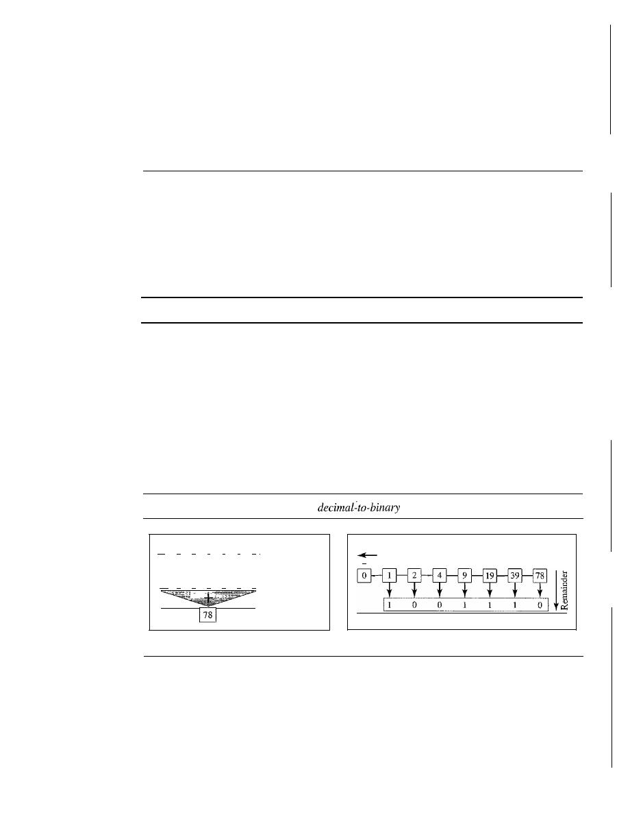
1038
APPENDIX B
NUMBERING SYSTEMS
Weights
In the decimal system, each weight equals 10 raised to the power of its position. The
weight of the symbol at position 0 is
100
(1);
the weight of the symbol at position 1 is
10
1
(10); and so on.
B.2
BASE 2: BINARY
The binary number system provides the basis for all computer operations. Computers
work by turning electric current on and off. The binary system uses two symbols, 0 and
1, so it corresponds naturally to a two-state device, such as a switch, with 0 to represent
the off state and 1 to represent the on state. The word
binary derives from the Latin
stem
bi, meaning 2.
Binary numbers use two symbols: 0 and 1.
Weights
In the binary system, each weight equals 2 raised to the power of its position. The
weight of the symbol at position 0 is
20 (1);
the weight of the symbol at position 1 is
2
1
(2);
and so on.
Conversion
Now let us see how we can convert binary to decimal and decimal to binary. Figure B.2
show the two processes.
Figure B.2
Binary-to-decimal and
conversion
11
0
0
1
1
1
0
I
Binary number
64 32 16
8
4
2
1 Weights
64
0
0
8
4
2
0 Weighted results
Decimal number
a. Binary to decimal
Q_uo_ti_en_ts
Decimal
number
1 0 0 1 1 1
0
Binary number
b. Decimal
to
binary
To convert a binary number to decimal, we use the weights. We multiply each symbol
by its weight and add all the weighted results. Figure B.2 shows how we can change
binary 1001110 to its decimal equivalent 78.
A simple division trick gives us a convenient way to convert a decimal number to
its binary equivalent, as shown in Figure B .2. To convert a number from decimal to
binary, divide the number by 2 and write down the remainder
(l
or 0). That remainder
is the least significant binary digit. Now, divide the quotient of that division by 2 and
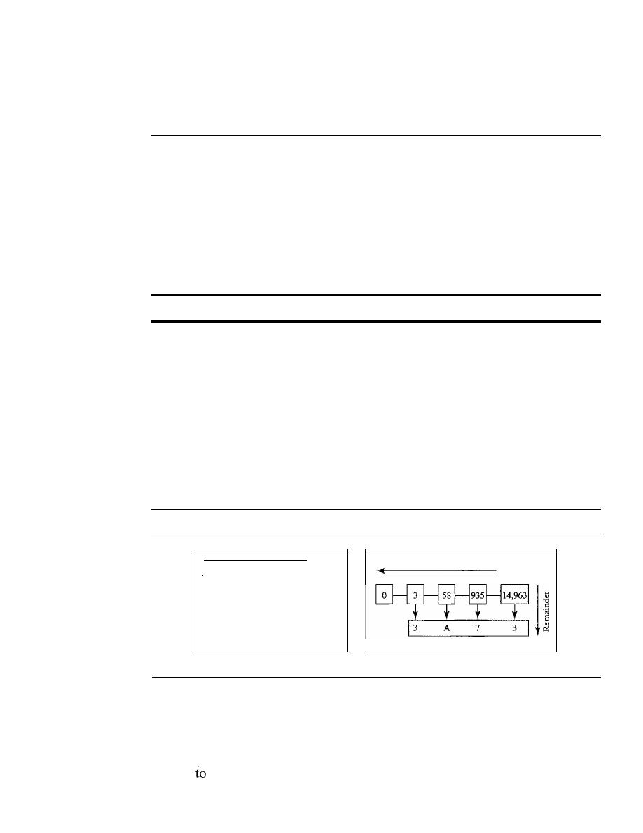
APPENDIX B
NUMBERING SYSTEMS
1039
write down the new remainder in the second position. Repeat this process until the quo-
tient becomes zero.
B.3
BASE 16: HEXADECIMAL
Another system used in this text is base 16. The term
hexadecimal
is derived from the
Greek term
hexadec,
meaning 16. The hexadecimal number system is convenient for
identifying a large binary number in a shorter form. The hexadecimal system uses
16 symbols: 0, 1, ... , 9, A, B, C, D, E, and
F.
The hexadecimal system uses the same
first 10 symbols as the decimal system, but instead of using 10, 11, 12, 13, 14, and
15, it uses A, B, C, D, E, and
F.
This prevents any confusion between two adjacent
symbols.
Hexadecimal numbers use 16 symbols: 0, 1, 2, 3, 4, 5, 6, 7, 8, 9, A, B, C, D, E, and F.
Weights
In the hexadecimal system, each weight equals 16 raised to the power of its position.
The weight of the symbol at position 0 is 16° (1); the weight of the symbol at position 1 is
16
1
(16); and so on.
Conversion
Now let us see how we can convert hexadecimal to decimal and decimal to hexadecimal.
Figure B.3 show the two processes.
Figure B.3
Hexadecimal-to-decimal and decimal-to-hexadecimal conversion
Quotients
I
3
4,096
A
256
7
16
Decimal
number
Hexadecimal number
a. Hexadecimal to decimal
b. Decimal to hexadecimal
To convert a hexadecimal number to decimal, we use the weights. We multiply
each symbol by its weight and add all the weighted results. Figure B.3 shows how
hexadecimal Ox3A73 is transformed to its decimal equivalent 14,963.
We use the same trick we used for changing decimal to binary to transform a
decimal
hexadecimal. The only difference is that we divide the number by 16 instead
of 2. The figure also shows how 14,963 in decimal is converted to hexadecimal Ox3A73.

1040
APPENDIX B
NUMBERING SYSTEMS
A Comparison
Table B.l shows how systems represent the decimal numbers 0 through 15. As you can
see, decimal 13 is equivalent to binary 1101, which is equivalent to hexadecimal
D.
Table B.I
Comparison of three systems
Decimal
Binary
Hexadecimal
0
0
0
1
1
1
2
10
2
3
11
3
4
100
4
5
101
5
6
110
6
7
111
7
Decimal
Binary
Hexadecimal
8
1000
8
9
1001
9
10
1010
A
11
1011
B
12
1100
C
13
1101
D
14
1110
E
15
1111
F
B.4
BASE 256: IP ADDRESSES
One numbering system that is used in the Internet is base 256. IPv4 addresses use this
base to represent an address in dotted decimal notation. When we define an IPv4
address as 131.32.7.8, we are using a base-256 number. In this base, we could have
used 256 unique symbols, but remembering that many symbols and their values is bur-
densome. The designers of the IPv4 address decided to use decimal numbers 0 to 255
as symbols and to distinguish between the symbols, a dot is used. The dot is used to
separate the symbols; it marks the boundary between the positions. For example, the
IPv4 address 131.32.7.8 is made of the four symbols 8, 7, 32, and 131 at positions 0, 1,2,
and 3, respectively.
IPv4 addresses use the base-256 numbering system.
The symbols
in
1Pv4 are decimal numbers between 0 and 255;
the separator is a dot.
Weights
In base 256, each weight equals 256 raised to the power of its position. The weight of
the symbol at position 0 is 256
0
(1);
the weight of the symbol at position 1 is 256
1
(256); and so on.
Conversion
Now let us see how we can convert hexadecimal to decimal and decimal to hexadecimal.
Figure B.4 show the two processes.
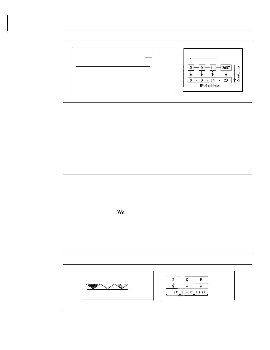
APPENDIX B
NUMBERING SYSTEMS
1041
Figure B.4
IPv4 address to decimal transformation
12,215,708,6861
Decimal number
_ _1_3_2
1_7
8
14_1 IPv4 address
256
3
256
2
256
1
256
0
Weights
2,214,592,512 1,114,112
2,048
14
Results
Quotients
Decimal
number
a. IP address to decimal
b. Decimal to IP address
To convert an IPv4 address to decimal, we use the weights. We multiply each symbol
by its weight and add all the weighted results. The figure shows how the IPv4 address
131.32.7.8 is transformed to its decimal equivalent.
We use the same trick we used for changing decimal to binary to transform a decimal
to an IPv4 address. The only difference is that we divide the number by 256 instead of 2.
However, we need to remember that the IPv4 address has four positions. This means
that when we are dealing with an IPv4 address, we must stop after we have found four
values. Figure
BA
shows an example for an IPv4 address.
B.5
OTHER CONVERSIONS
There are other transformations such as base 2 to base 16 or base 16 to base 256.
It
is
easy to use base 10 as the intermediate system. In other words, to change a number
from binary to hexadecimal we first change the binary to decimal and then change the
decimal to hexadecimal.
discuss some easy methods for common transformations.
Binary and Hexadecimal
There is a simple way to convert binary to hexadecimal and vice versa as shown in
Figure B.5.
Figure B.5
Transformation from binary to hexadecimal
I
1 0 ]1 000 11 1 1 0
I
Binary
2
8
E
Hexadecimal
a. Binary to hexadecimal
Hexadecimal
Binary
b. Hexadecimal to binary
To change a number from binary to hexadecimal, we group the binary digits from
the right by fours. Then we convert each 4-bit group to its hexadecimal equivalent,

1042
APPENDIX B
NUMBERING SYSTEMS
using Table B.1. In the figure, we convert binary 1010001110 to hexadecimal Ox28E.
To change a hexadecimal number to binary, we convert each hexadecimal digit to its
equivalent binary number, using Table B.1, and concatenate the results. In Figure B.5
we convert hexadecimal Ox28E to binary.
Base 256 and Binary
To convert a base 256 number to binary, we first need to convert the number in each
position to an 8-bit binary group and then concatenate the groups. To convert from
binary to base 256, we need to divide the binary number into groups of 8 bits, convert
each group to decimal, and then insert separators (dots) between the decimal numbers.
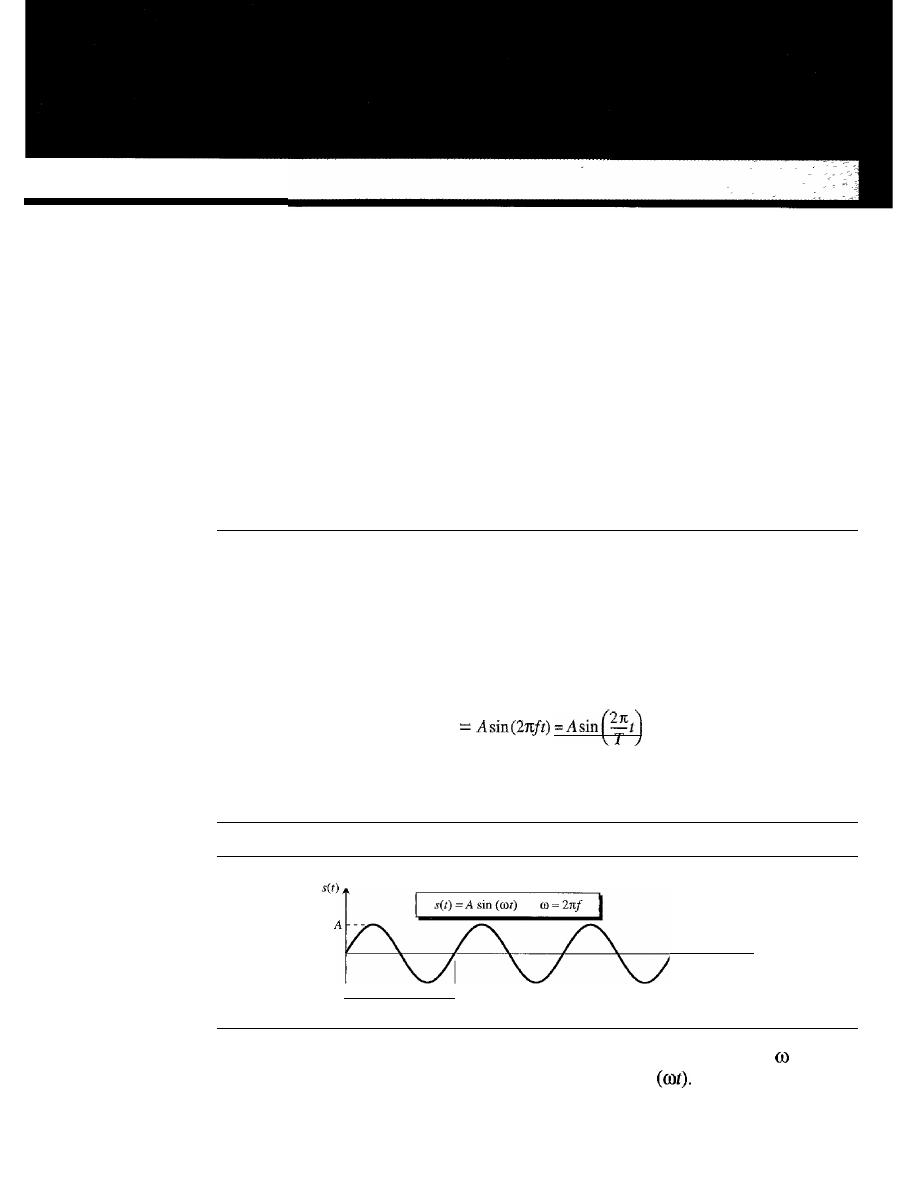
APPENDIXC
Mathematical Review
In
this appendix, we review some mathematical concepts that may help you to better
understand the topics covered in the book. Perhaps the most important concept in data
communications is signals and their representation. We start with a brief review of trig-
onometric functions, as discussed in a typical precalculus book. We then briefly discuss
Fourier analysis, which provides a tool for the transformation between the time and fre-
quency domains. We finally give a brief treatment of exponential and logarithmic functions.
C.l
TRIGONOMETRIC FUNCTIONS
Let us briefly discuss some characteristics of the trigonometric functions as used in the
book.
Sine Wave
We can mathematically describe a sine wave as
set)
where s is the instantaneous amplitude, A is the peak amplitude,
f
is the frequency, and
T
is the period (phase will be discussed later). Figure C.l shows a sine wave.
Figure C.I
A
sine wave
Time
T
Note that the value of 21tfis called the radian frequency and written as
(omega),
which means that a sine function can written as
set)
=
A
sin
1043
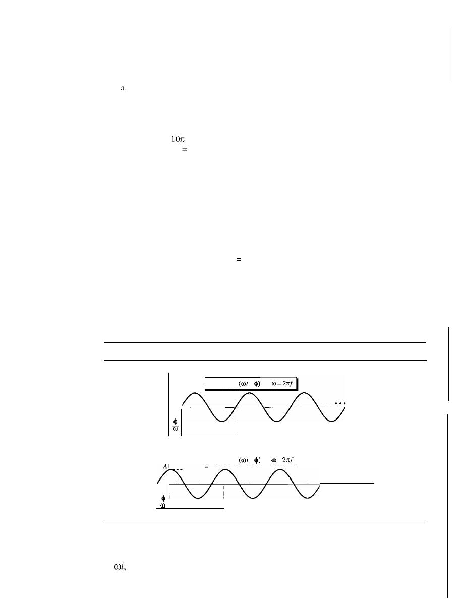
1044
APPENDIX C
MATHEMATICAL REVIEW
Example C.l
Find the peak value, frequency, and period of the following sine waves.
set)
=
5 sin (10m)
b.
set)
=
sin
(lOt)
Solution
a. Peak amplitude:
A
=
5
Frequency:
=
2rtf, sof= 5
Period:
T
=
IIJ
1/5 s
b.
Peak amplitude:
A
=
1
Frequency: 10
=
2rtf,
so f
=
1O/(2rt)
=
1.60
Period:
T
=
IIJ
=
1/1.60
=
0.628
s
Example
C.2
Show the mathematical representation of a sine wave with a peak amplitude of
2 and a frequency
of 1000 Hz.
Solution
The mathematical representation is
set)
2 sin
(20001tt).
Horizontal Shifting (Phase)
All the sine functions we discussed so far have an amplitude of value 0 at the origin.
What if we shift the signal to the left or to the right? Figure C.2 shows two simple sine
waves, one shifted to the right and one to the left.
Figure C.2
Two horizontally shifted sine waves
I
s(t)
=A sin
-
A
- --
Time
T
I
s(t)
=
A
sin
+
=
I
...
Time
T
When a signal is shifted to the left or right, its first zero crossing will be at a point
in time other than the origin. To show this, we need to add or subtract another constant
to
as shown in the figure.
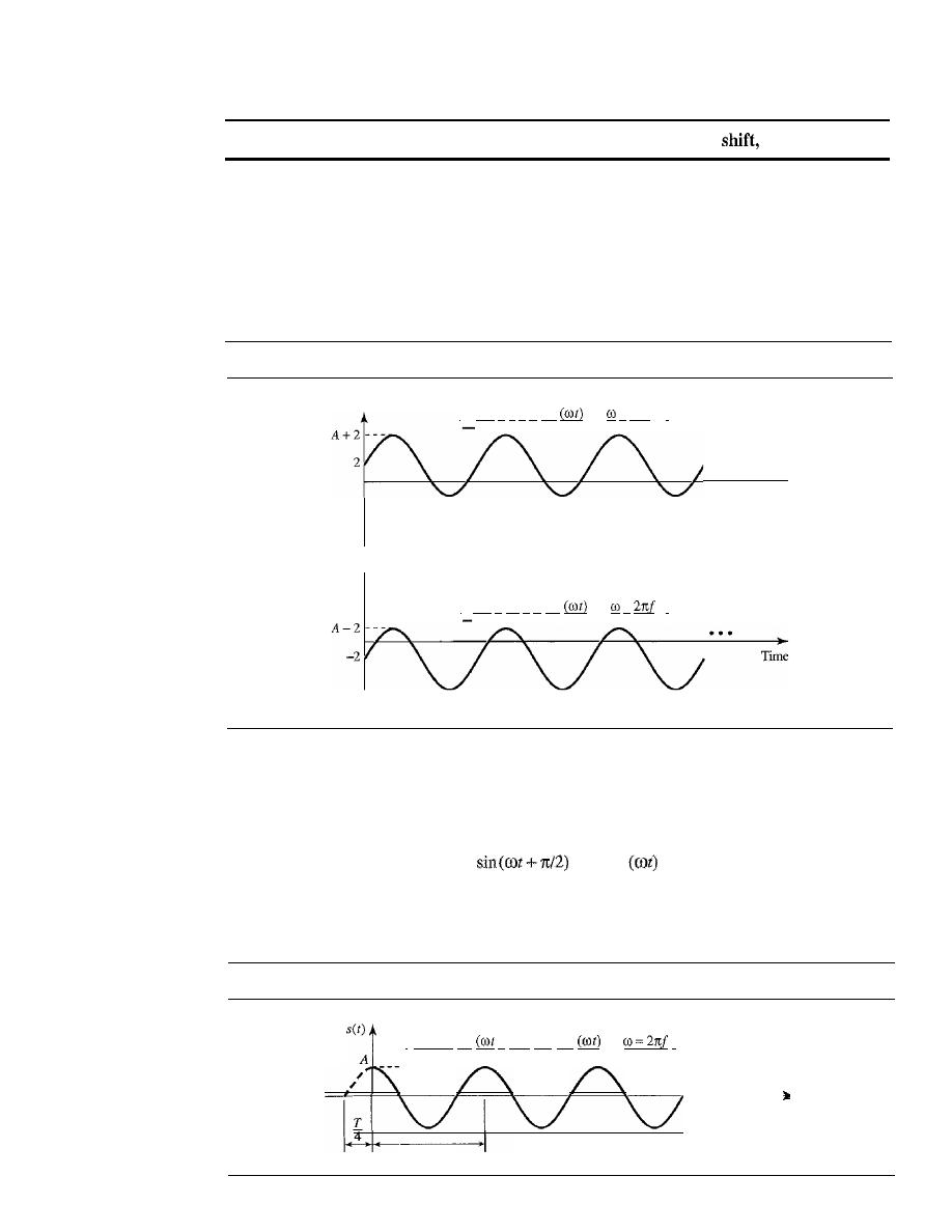
APPENDIX
C
MATHEMATICAL REVIEW
1045
Shifting a sine wave to the left or right is a positive or negative
respectively.
Vertical Shifting
When a sine wave is shifted vertically, a constant is added to the instantaneous ampli-
tude of the signal. For example, if we shift a sine wave 2 units of amplitude upward, the
signal becomes
set)
=
2
+
sin (rot); if we shift it 2 units of amplitude downward, we have
set)
=
-2
+
sin (rot). Figure C.3 shows the idea.
Figure C.3
Vertical shifting of sine waves
I
s(t)
=
2
+
A
sin
=
2rrf
I
Time
I
s(t)
=
-2
+
A
sin
=
I
Cosine Wave
If
we shift a sine wave
T/2
to the left, we get what is called a cosine wave (cos).
A
=A
cos
Figure C.4 shows a cosine wave.
Figure C.4
A cosine wave
I
s(t)=A
sin
+
T/4) =A
cos
I
---
4
T
Time
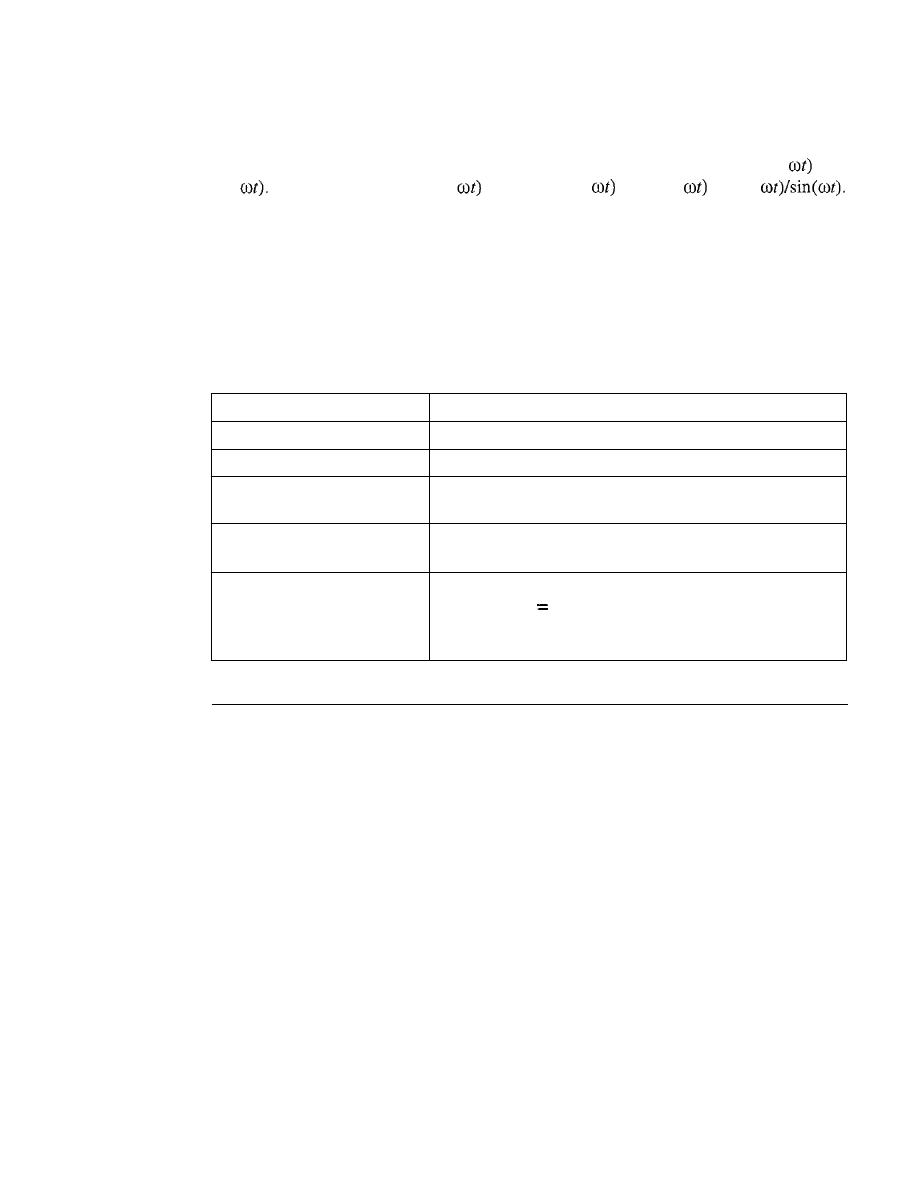
1046
APPENDIX C
MATHEMATICAL REVIEW
Other Trigonometric Functions
There are many trigonometric functions; two of the more common are tan(
and
cot(
They are defined as tan(
=
sine
(Ot)/cos(
and cot(
=
cos(
Note that tan and cot are the inverse of each other.
Trigonometric Identities
There are several identities between trigonometric functions that we sometimes need to
know. Table C.l gives these identities for reference. Other identities can be easily
derived from these.
Table C.l
Some trigonometric identities
Name
Formula
Pythagorean
sin
2
x
+
cos
2
x
=
1
Even/odd
sin
(-x)
=
-sin
(x)
cos
(-x)
=
cos
(x)
Sum
sin
(x
+
y)
=
sin
(x)
cos
(y)
+
cos
(x)
sin
(y)
cos
(x
+
y)
=
cos
(x)
cos
(y) -
sin(x)
sin(y)
Difference
sin
(x - y)
=
sin
(x)
cos
(y) -
cos
(x)
sin
(y)
cos
(x - y)
=
cos
(x)
cos (Y)
+
sin
(x)
sin
(y)
Product to sum
sin
(x)
sin
(y)
=
1/2 [cos
(x- y) -
cos
(x
+
y)]
cos
(x)
cos
(y)
1/2 [cos
(x - y)
+
cos
(x
+
y)]
sin
(x)
cos
(y)
=
1/2 [sin
(x
+
y)
+
sin
(x - y)]
cos
(x)
sin
(y)
=
1/2 [sin
(x
+
y) -
sin
(x - y)]
C.2
FOURIER
ANALYSIS
Fourier analysis is a tool that changes a time-domain signal to a frequency-domain signal
and vice versa.
Fourier Series
Fourier proved that a composite periodic signal with period
T
(frequency f) can be
decomposed into a series of sine and cosine functions in which each function is an
integral harmonic of the fundamental frequency
f
of the composite signal. The result is
called the
Fourier
series. In other words, we can write a composite signal as shown in
Figure C.S. Using the series, we can decompose any periodic signal into its harmonics.
Note that
A
o
is the average value of the signal over a period,
An
is the coefficient of the
nth cosine component, and
B
n
is the coefficient of the
nth sine component.
Example
C.3
Let us show the components of a square wave signal as seen in Figure C.6. The figure also shows
the time domain and the frequency domain. According to the figure, such a square wave signal has
only An coefficients. Note also that the value ofA
o
=
0 because the average value of the signal is 0;
it is oscillating above and below the time axis. The frequency domain of the signal is discrete;
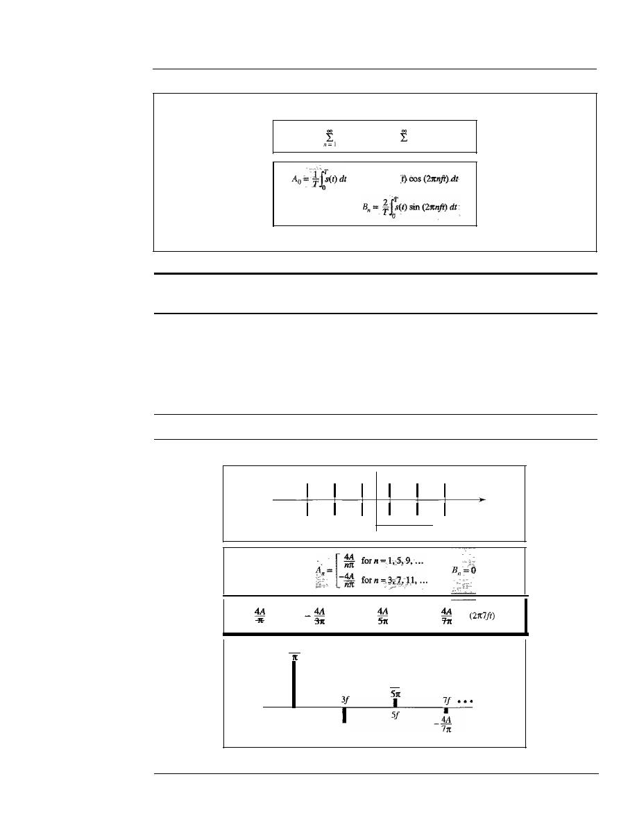
APPENDIX
C
MATHEMATICAL REVIEW
1047
Figure C.S
Fourier series and coefficients oftenns
Fourier series
s(t)
=
A
o +
All
sin
(21tnft)
+
B"
cos
(21tnft)
n=l
Coefficients
Fourier series
Time domain: periodic
Frequency domain: discrete
only odd harmonics are present and the amplitudes are alternatively positive and negative. A very
important point is that the amplitude of the harmonics approaches zero as we move toward infin-
ity. Something which is not shown in the figure is the phase. However, we know that all compo-
nents are cosine waves, which means that each has a phase of 90°.
Figure C.6
Finding the Fourier series of a periodic square function
Time domain
Time
o
A
-A
T
Ao=O
set)
=
cos
(21tft)
cos
(21t3ft)
+
cos
(21t5ft) -
cos
+ •••
4A
f
4A
31t
4A
Frequency
Frequency domain
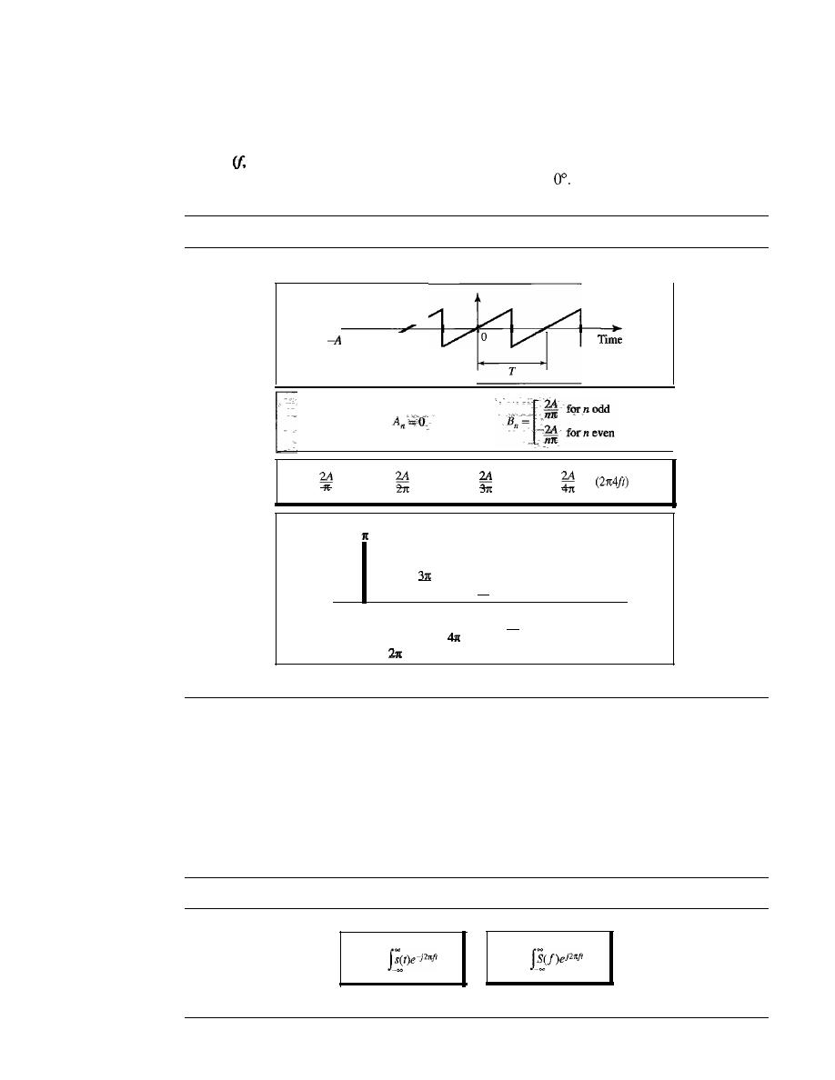
1048
APPENDIX
C
MATHEMATICAL REVIEW
Example
C.4
Now let us show the components of a sawtooth signal as seen in Figure C.7. This time, we have
only
En
components (sine waves). The frequency spectrum, however, is denser; we have all har-
monics
2j, 3j, ... ).
A point which is not clear from the diagram is the phase. All components
are sine waves, which means each component has a phase of
Figure
C.
7
Finding the Fourier series for a sawtooth signal
Time domain
I
A
•••
set)
=
sin
(2rcft) -
sin
(2rc2ft)
+
sin
(21t3ft) -
sin
+ •••
2A
f
21
I
2A
-
2A
I
4f
3f
I
2A
-
2A
5
1
1t
6f
5f'
2A
-
61t
Frequency
Frequency domain
Fourier Transform
While the Fourier series gives the discrete frequency domain of a periodic signal, the
Fourier transform
gives the continuous frequency domain of a nonperiodic signal.
Figure C.S shows how we can create a continuous frequency domain from a nonperiodic
time-domain function and vice versa.
Figure C.S
Fourier transform and inverse Fourier transform
S(f)
=
dt
set)
=
dt
Fourier transform
Inverse Fourier transform
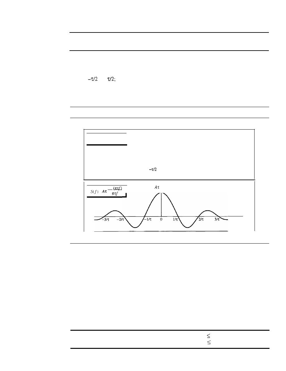
APPENDIX
C
MATHEMATICAL REVIEW
1049
Fourier transform
Time domain: nonperiodic
Frequency domain: continuous
Example
C.s
Figure C.9 shows the time and frequency domains of one single square pulse. The time domain is
between
and
the frequency domain is a continuous function that stretches from negative
infinity to positive infinity. Unlike the previous examples, the frequency domain is continuous; all
frequencies are there, not just the integral ones.
Figure C.9
Finding the Fourier transform of a square pulse
Time domain
0
1;/2
sin
=
Frequency domain
Frequency
Time-Limited and Band-Limited Signals
Two very interesting concepts related to the Fourier transform are the time-limited
and band-limited signals. A time-limited signal is a signal for which the amplitude of
set)
is nonzero only during a period of time; the amplitude is zero everywhere else.
A band-limited signal, on the other hand, is the signal for which the amplitude of
Sif)
is nonzero only for a range of frequencies; the amplitude is zero everywhere else. A
band-limited signal plays a very important role in the sampling theorem and Nyquist
frequency because the corresponding time domain can be represented as a series of
samples.
Time-limited signal:
s(t)
=
0 for I
t
I
T
Band-limited signal: Sif)
=
0 for If I
B

1050
APPENDIX C
MATHEMATICAL REVIEW
C.3
EXPONENT AND LOGARITHM
In solving networking problems, we often need to know how to handle exponential and
logarithmic functions. This section briefly reviews these two concepts.
Exponential Function
The exponential function with base
a
is defined as
If
x is an integer (integral value), we can easily calculate the value of
y
by multiplying
the value of
a
by itself
x
times.
Example
C.6
Calculate the value of the following exponential functions.
a.
y
=
3
2
b.
Y
=
5.2
6
Solution
a. y=
3
x
3 =9
b.
y
=
5.2
x
5.2
x
5.2
x
5.2
x
5.2
x
5.2
=
19,770.609664
If
x is not integer, we need to use a calculator.
Example
C.7
Calculate the value of the following exponential functions.
a.
y
=
3
2.2
b.
y
=
5.2
6
.3
Solution
a.
y
=
11.212 (approximately)
b.
y
=
32,424.60 (approximately)
Natural Base
One very common base used in science and mathematics is the natural base
e,
which
has the value 2.71828183.... Most calculators show this function as
which can be
calculated easily by entering only the value of the exponent.
Example
C.s
Calculate the value of the following exponential functions.
_
4
a.
y-e
b.
y
=
e
6
.3
Solution
a.
y
=
54.56 (approximately)
b.
y
=
544.57 (approximately)
APPENDIX
C
MATHEMATICAL REVIEW
1051
Properties of the Exponential Function
Exponential functions have several properties; some are useful to us in this text:
First:
Second:
Third:
y
=
1
y
=a1 =a
Example C.9
The third property is useful to us because we can calculate the value of an exponential function
with a negative value. We first calculate the positive value and we then invert the result.
a.
y
e-
4
b.
y
e-6·3
Solution
a.
y
1/ 54.56
=
0.0183
b. y
=
1/ 544.57
=
0.00183
Logarithmic Function
A logarithmic function is the inverse of an exponential function, as shown below. Just
as in the exponential function,
a
is called the base of the logarithmic function:
y
x
=
In other words, if
x
is given, we can calculate y by using the exponential
if
y
is given, we can calculate
x
by using the logarithmic function.
Exponential and logarithmic functions are the inverse of each other.
Example C.10
Calculate the value of the following logarithmic
a.
x
=
log3 9
b. x
=
log2 16
Solution
We have not yet shown how to calculate the log function in different bases, but we can solve this
problem intuitively.
a. Because 32
9, we can say that log3 9
=
2, using the fact that the two functions are the
inverse of each other.
b. Because
2
4
=
16, we can say that log2l6
=
4 by using the previous fact.
Two Common Bases
The two common bases for logarithmic functions, those that can be handled by a calcu-
lator, are base
e
and base 10. The logarithm in base
e
is normally shown as In (natural
logarithm); the logarithm in base 10 is normally shown as log (omitting the base).

1052
APPENDIX
C
MATHEMATICAL REVIEW
Example Cll
Calculate the value of the following logarithmic functions.
a.
x
=
log 233
b.
x
=
In 45
Solution
For these two bases we can use a calculator.
a.
x
=
log 233
=
2.367
b.
x
=
In 45
=
3.81
Base Transformation
We often need to find the value of a logarithmic function in a base other than
e
or 10. If
the available calculator cannot give the result in our desired base, we can use a very
fundamental property of the logarithm, base transformation, as shown:
10gb
Y
- -
10gb
a
Note that the right-hand side is two log functions with base
b,
which is different
from the base a at the left-hand side. This means that we can choose a base that is
available in our calculator (base
b)
and find the log of a base that is not available
(base
a).
Example C12
Calculate the value of the following logarithmic functions.
a. x
=
log3 810
b.
x
=
log5
600
Solution
These two bases, 3 and 5, are not available on a calculator, but we can use base 10 which is available.
loglO 810
2.908
a.
x
=
log3 810
=
= - -
=
6.095
log 10
3
0.477
log 10
600
2.778
b. x
=
log5
600
=
= - -
=
3.975
log
10 5
0.699
Properties of Logarithmic Functions
Like an exponential function, a logarithmic function has some properties that are useful
in: simplifying the calculation of a log function.
First:
Second:
Third:
1
=
0
a
=
1
!
=
x
x
Fourth:
Fifth:
Sixth:
(x xY)
=
x
+
=
x -
y
y
x
Y
=
Y x
x

APPENDIX C
MATHEMATICAL REVIEW
1053
Example C13
Calculate the value of the following logarithmic functions.
a.
x
=
log3 1
b.
x
=
log3
3
c.
x
=
loglO (l/10)
d. loga
(x
x
y)
if we know that loga
x
=
2 and loga
y
=
3
e. logz (1024) without using a calculator
Solution
We use the property of log functions to solve the problems.
a.
x
=
log3 1
=
0
b. x
=
log3
3
=
1
c. x
=
loglO (1110)
=
loglOlO-l
=
-loglO 10
=
-1
d. loga
(x
x
y)
=
loga x
+
loga
Y
=
2
+
3
=
5
e.
10g
z
(1024)
=
logz (2
10
)
=
10 logz 2
=
10 x 1
=
10


APPENDIXD
8B/6TCode
This appendix is a tabulation of 8B/6T code pairs. The 8-bit data are shown in hexadecimal
format. The 6T code is shown as
+
(positive signal), - (negative signal), and 0 (lack of
signal) notation.
Table
D.l
8B/6T code
Data
Code
Data
Code
Data
Code
Data
Code
00
-+00-+
20
-++-00
40
-00+0+
60
0++0-0
01
0-+-+0
21
+00+--
41
0-00++
61
+0+-00
02
0-+0-+
22
-+0-++
42
0-0+0+
62
+0+0-0
03
0-++0-
23
+-0-++
43
0-0++0
63
+0+00-
04
-+0+0-
24
+-0+00
44
-00++0
64
0++00-
05
+0--+0
25
-+0+00
45
00-0++
65
++0-00
06
+0-0-+
26
+00-00
46
00-+0+
66
++00-0
07
+0-+0-
27
-+++--
47
00-++0
67
++000-
08
-+00+-
28
0++-0-
48
00+000
68
0++-+-
09
0-++-0
29
+0+0--
49
++-000
69
+0++--
OA
0-+0+-
2A
+0+-0-
4A
+-+000
6A
+0+-+-
OB
0-+-0+
2B
+0+--0
4B
-++000
6B
+0+--+
OC
-+0-0+
2C
0++--0
4C
0+-000
6C
0++--+
OD
+0-+-0
2D
++00--
4D
+0-000
6D
++0+--
OE
+0-0+-
2E
++0-0-
4E
0-+000
6E
++0-+-
OF
+0--0+
2F
++0--0
4F
-0+000
6F
++0--+
10
0--+0+
30
+-00-+
50
+--+0+
70
000++-
11
-0-0++
31
0+--+0
51
-+-0++
71
000+-+
12
-0-+0+
32
0+-0-+
52
-+-+0+
72
000-++
13
-0-++0
33
0+-+0-
53
-+-++0
73
000+00
1055

1056
APPENDIX D
8B/6T CODE
Table D.I
8B/6T code (continued)
Data
Code
Data
Code
Data
Code
Data
Code
14
34
54
+--++0
74
000+0-
15
--00++
35
-0+-+0
55
75
000+-0
16
--0+0+
36
-0+0-+
56
--++0+
76
000-0+
17
--0++0
37
-0++0-
57
--+++0
77
000-+0
18
-+0-+0
38
+-00+-
58
--0+++
78
+++--0
19
+-0-+0
39
59
-0-+++
79
+++-0-
lA
-++-+0
3A
0+-0+-
5A
0--+++
7A
+++0-
IB
+00-+0
3B
0+--0+
5B
0--0++
7B
0++0- -
lC
+00+-0
3C
5C
+--0++
7C
-00-++
ID
-+++-0
30
-0++-0
50
-000++
7D
-00+00
IE
3E
-0+0+-
5E
0+++--
7E
+- --++
IF
-+0+-0
3F
-0+-0+
5F
0++-00
7F
+- -+00
80
-00+-+
AO
-++0-0
CO
-+0+-+
EO
-++0-+
81
0-0-++
Al
+-+-00
Cl
0-+-++
El
+-++0
82
0-0+-+
A2
+-+0-0
C2
0-++-+
E2
+-+0-+
83
A3
C3
0-+++-
E3
+-++0-
84
-00++-
A4
-++00-
C4
E4
-+++0-
85
00--++
A5
++--00
C5
+0--++
E5
++--+0
86
00-+-+
A6
++-0-0
C6
+0-+-+
E6
++-0-+
87
A7
C7
+0-++-
E7
88
-000+0
A8
-++-+-
C8
-+00+0
E8
-++0+-
89
0-0+00
A9
+-++--
C9
0-++00
E9
+-++-0
8A
0-00+0
AA
CA
0-+0+0
EA
8B
0-000+
AB
+-+--+
CB
0-+00+
EB
+-+-0+
8C
-0000+
AC
-++--+
CC
-+000+
EC
-++-0+
80
00-+00
AD
++-+--
CD
+0-+00
ED
++-+-0
8E
00-0+0
AE
++--+-
CE
+0-0+0
EE
++-0+-
8F
00-00+
AF
++---+
CF
+0-00+
EF
++--0+
90
+--+-+
BO
+000-0
DO
+-0+-+
FO
+000-+
91
-+--++
Bl
0+0-00
01
0+--++
Fl
0+0-+0
92
B2
0+00-0
02
0+-+-+
F2
0+00-+
93
-+-++-
B3
0+000-
D3
0+-++-
F3
0+0+0-
94
+--++-
B4
+0000-
D4
+-0++-
F4
+00+0-

Table D.I
8B/6Tcode (continued)
APPENDIX
D
8B/6T CODE
1057
Data
Code
Data
Code
Data
Code
Data
Code
95
--+-++
B5
00+-00
05
-0+-++
F5
00+-+0
96
B6
00+0-0
06
-0++-+
F6
00+0-+
97
--+++-
B7
00+00-
07
-0+++-
F7
00++0-
98
+--0+0
B8
+00-+-
08
+-00+0
F8
+000+-
99
-+-+00
B9
0+0+--
09
0+-+00
F9
0+0+-0
9A
-+-0+0
BA
0+0-+-
OA
0+-0+0
FA
0+00+-
9B
-+-00+
BB
0+0--+
OB
0+-00+
FB
0+0-0+
9C
+--00+
BC
+00--+
OC
+-000+
FC
+00-0+
90
--++00
BO
00++--
00
-0++00
FD
00++-0
9E
--+0+0
BE
00+-+-
OE
-0+0+0
FE
00+0+-
9F
--+00+
BF
00+--+
OF
-0+00+
FF
00+-0+

APPENDIXE
Telephone History
In Chapter 9, we discussed telephone networks. In this appendix, we briefly review the
history of telephone networks. The history in the United States can be divided into three
eras: prior to 1984, between 1984 and 1996, and after 1996.
Before 1984
Before 1984, almost all local and long-distance services were provided by the AT&T Bell
System. In 1970, the U.S. government, believing that the Bell System was monopolizing
the telephone service industry, sued the company. The verdict was in favor of the govern-
ment and resulted in a document called the Modified Final Judgment (MFJ). Beginning on
January 1, 1984, AT&T was broken into AT&T Long Lines, 23 Bell Operating Compa-
nies (BOCs), and others. The 23 BOCs were grouped to make several Regional Bell
Operating Companies (RBOSs). This landmark event, the AT&T divestiture of 1984, was
beneficial to customers of telephone services. Telephone rates were lowered.
Between 1984 and 1996
The divestiture divided the country into more than 200 LATAs; some companies were
allowed to provide services inside a LATA (LECs), and others were allowed to provide
services between LATAs (IXCs). Competition, particularly between long-distance car-
riers, increased as new companies were formed. However, no LEC could provide long-
distance services, and no IXCs could provide local services.
After 1996
Another major change in telecommunications occurred in 1996. The Telecommunica-
tions Act of 1996 combined the different services provided by different companies
under the umbrella of telecommunication services; this included local services, long-
distance voice and data services, video services, and so on. In addition, the act allowed
any company to provide any of these services at the local and long-distance levels. In
other words, a common carrier company provides services both inside the LATA and
between the LATAs. However, to prevent the recabling of residents, the carriers that were
given intra-LATA services (ILECs) continued to provide the main services; the new
competitors (CLECs) provided other services.
1059


APPENDIXF
Contact Addresses
The following is a list of contact addresses for various organizations mentioned in
the text.
o
ATMForum
Presidio of San Francisco
P.O. Box 29920 (mail)
572B Ruger Street (surface)
San Francisco, CA 94129-0920
Telephone: 415 561-6275
E-mail: info@atmforum.com
www.atmforum.com
o
Federal Communications Commission
(FCC)
445 12th Street S.W.
Washington, DC 20554
Telephone: 1-888-225-5322
E-mail: fccinfo@fcc.gov
www.fcc.gov
o
Institute of Electrical and Electronics Engineers (IEEE)
Operations Center
445 Hoes Lane
Piscataway, NJ 08854-1331
Telephone: 732981-0060
www.ieee.org
1061

1062
APPENDIX F
CONTACT ADDRESSES
o
International Organization for Standardization (ISO)
1, rue de Varembe
Caisse Posta1e 56
CH-1211 Geneve 20
Switzerland
Telephone: 41 227490111
E-mail: central@iso.ch
www.iso.org
o
International Telecommunication Union (ITU)
Place des Nations
CH-1211 Geneva 20
Switzerland
Telephone: 41 22 730 5852
E-mail: tsbmail@itu.int
www.itu.intlhome
o
Internet Architecture Board (lAB)
E-mail: lAB @isi.edu
www.iab.org
o
Internet Corporation for Assigned Names and Numbers (ICANN)
4676 Admiralty Way, Suite 330
Marina del Rey, CA 90292-6601
Telephone: 310 823-9358
E-mail: icann@icann.org
www.icann.org
o
Internet Engineering Steering Group (IESG)
E-mail: iesg@ietf.org
www.ietf.org/iesg.html
o
Internet Engineering Task Force (IETF)
E-mail: ietf-infor@ietf.org
www.ietf.org
o
Internet Research Task Force (IRTF)
E-mail: irtf-chair@ietf.org
www.irtf.org
o
Internet Society (ISOC)
1775 Weihle Avenue, Suite 102
Reston, VA 20190-5108
Telephone: 703.326-9880
E-mail: info@isoc.org
www.isoc.org

APPENDIXG
RFCs
In Table G.1, we list alphabetically by protocol the RFCs that are directly related to
the material in this text. For more information go to the following site: http://
www.rfc-editor.org.
Table G.t
RFCs for each protocol
Protocol
RFC
ARPandRARP
826,903,925,1027,1293,1329,1433,1868,1931,2390
BGP
1092,1105,1163,1265,1266,1267,1364,1392,1403,1565,
1654,1655,1665,1771,1772,1745,1774,2283
BOOTP and DHCP
951, 1048, 1084, 1395, 1497, 1531, 1532, 1533, 1534, 1541,
1542,2131,2132
CIDR
1322,1478,1479,1517,1817
DHCP
See BOOTP and DHCP
DNS
799,811,819,830,881,882,883,897,920,921,1034,1035,
1386,1480,1535,1536,1537,1591,1637,1664,1706,1712,
1713,1982,2065,2137,2317,2535,2671
FTP
114,133,141,163,171,172,238,242,250,256,264,269,281,
291,354,385,412,414,418,430,438,448,463,468,478,486,
505,506,542,553,624,630,640,691,765,913,959,1635,
1785,2228,2577
HTML
1866
HTTP
2068,2109
ICMP
777,792,1016,1018,1256,1788,2521
IGMP
966,988,1054,1112,1301,1458,1469,1768,2236,2357,2365,
2502,2588
IMAP
See SMTP, MIME, POP, IMAP
IP
760,781,791,815, 1025, 1063, 1071, 1141, 1190, 1191,
1624,2113
1063

1064
APPENDIX
G
RFCs
Table G.!
RFCsfor each protocol (continued)
Protocol
RFC
IPv6
1365,1550,1678, 1680,1682,1683,1686,1688,1726,1752,
1826,1883,1884,1886,1887,1955,2080,2373,2452,2463,
2465,2466,2472,2492,2545,2590
MIB
See SNMP, MIB, SMI
MIME
See SMTP, MIME, POP, IMAP
Multicast Routing
1584,1585,2117,2362
NAT
1361,2663,2694
OSPF
1131,1245,1246,1247,1370,1583, 1584, 1585, 1586, 1587,
2178,2328,2329,2370
POP
See SMTP, MIME, POP, IMAP
RARP
See ARP and RARP
RIP
1131,1245,1246,1247,1370,1583, 1584, 1585, 1586, 1587,
1722,1723,2082,2453
SCTP
2960,3257,3284,3285,3286,3309,3436,3554,3708,3758
SMI
See SNMP, MIB, SMI
SMTP, MIME, POP,
196,221,224,278,524,539,753,772,780,806,821,934,974,
IMAP
1047, 1081, 1082, 1225, 1460, 1496, 1426, 1427, 1652, 1653,
1711,1725,1734,1740,1741,1767,1869,1870,2045,2046,
2047,2048,2177,2180,2192,2193,2221,2342,2359,2449,
2683,2503
SNMP, MIB, SMI
1065, 1067, 1098, 1155, 1157, 1212, 1213, 1229, 1231,1243,
1284, 1351, 1352, 1354, 1389, 1398, 1414, 1441,1442,1443,
1444, 1445, 1446, 1447, 1448, 1449, 1450, 1451, 1452, 1461,
1472, 1474, 1537, 1623, 1643, 1650, 1657, 1665, 1666, 1696,
1697, 1724, 1742, 1743, 1748, 1749
TCP
675,700,721,761,793,879,896,1078,1106,1110,1144,1145,
1146,1263,1323,1337,1379,1644,1693,1901,1905,2001,
2018,2488,2580
TELNET
137,340,393,426,435,452,466,495,513,529,562,595,596,
599,669,679,701,702,703,728,764,782,818,854,855,1184,
1205,2355
TFfP
1350, 1782, 1783, 1784
UDP
768
VPN
2547,2637,2685
WWW
1614, 1630, 1737, 1738

APPENDIXH
UDP and TCP Ports
Table H.I lists the common well-known ports ordered by port number.
Table
H.I
Ports by port number
Port Number
Protocol
7
TCP
ECHO
13
UDPrrCp
DAYTIME
19
UDPITCP
CHARACTER GENERATOR
20
TCP
FTP-DATA
21
TCP
FTP-CONTROL
23
TCP
TELNET
25
TCP
SMTP
37
UDPrrCp
TIME
67
UDP
BOOTP-SERVER
68
UDP
BOOTP-CLIENT
69
UDP
TFTP
70
TCP
GOPHER
79
TCP
FINGER
80
TCP
HTTP
109
TCP
POP-2
110
TCP
POP-3
111
UOPITCP
RPC
161
UOP
SNMP
162
UOP
SNMP-TRAP
179
TCP
BGP
520
UOP
RIP
1065

1066
APPENDIX H
UDP AND TCP PORTS
Table H.2 lists the ports, ordered alphabetically by protocol.
Table H.2
Port numbers by protocol
Protocol
UDPITCP
Port Number
BGP
TCP
179
BOOTP-SERVER
UDP
67
BOOTP-CLIENT
UDP
68
CHARACTER GENERATOR
UDP/TCP
19
DAYTIME
UDP/TCP
13
ECHO
TCP
7
FINGER
TCP
79
FTP-CONTROL
TCP
21
FTP-DATA
TCP
20
GOPHER
TCP
70
HTTP
TCP
80
POP-2
TCP
109
POP-3
TCP
110
RIP
UDP
520
RPC
UDP/TCP
111
SMTP
TCP
25
SNMP
UDP
161
SNMP-TRAP
UDP
162
TELNET
TCP
23
TFTP
UDP
69
TIME
UDP/TCP
37

Acronyms
AAL
application adaptation layer
BER
Basic Encoding Rules
ABM
asynchronous balanced mode
BOP
Border Gateway Protocol
ACK
acknowledgment
BNC
Bayone-Neill-Concelman
ACL
asynchronous connectionless link
BOOTP
Bootstrap Protocol
AOSL
asymmetric digital subscriber line
BSS
basic service set
AES
Advanced Encryption Standard
BUS
broadcast/unknown server
AH
Authentication Header
CA
Certification Authority
AM
amplitude modulation
CATV
community antenna TV
AMI
alternate mark inversion
CBC
cipher block chaining mode
AMPS
Advanced Mobile Phone System
CBR
constant bit rate
ANSI
American National Standards Institute
CBT
Core-Based Tree
AP
access point
CCITT
Consultative Committee for
ARP
Address Resolution Protocol
International Telegraphy and
ARPA
Advanced Research Projects Agency
Telephony
ARPANET
Advanced Research Projects Agency
CCK
complementary code keying
Network
COMA
code division multiple access
ARQ
automatic repeat request
CFB
cipher feedback mode
AS
authentication server
COl
Common Gateway Interface
AS
autonomous system
CHAP
Challenge Handshake Authentication
ASCII
American Standard Code for
Protocol
Information Interchange
CrOR
Classless InterDomain Routing
ASK
amplitude shift keying
CrR
committed information rate
ASN.l
Abstract Syntax Notation 1
CLEC
competitive local exchange carrier
ATM
Asynchronous Transfer Mode
CMTS
cable modem transmission system
AUr
attachment unit interface
CRC
cyclic redundancy check
B8ZS
bipolar with 8-zero substitution
CS
convergence sublayer
Be
committed burst size
CSM
cipher stream mode
Be
excess burst size
CSMA
carrier sense multiple access
BECN
backward explicit congestion
CSMAICA
carrier sense mUltiple access with
notification
collision avoidance
1067

1068
ACRONYMS
CSMA/CD
carrier sense multiple access with
FSK
frequency shift keying
collision detection
FTP
File Transfer Protocol
D-AMPS
digital AMPS
GPS
Global Positioning System
DARPA
Defense Advanced Research Projects
GSM
Global System for Mobile
Agency
Communication
dB
decibel
HDLC
High-level Data
Link
Control
DC
direct current
HDSL
high bit rate digital subscriber line
DCF
distributed coordination function
HFC
hybrid-fiber-coaxial network
OCT
discrete cosine transform
HMAC
hashed-message authentication code
DONS
Domain Name System
HR-DSSS
High Rate Direct Sequence Spread
DDS
digital data service
Spectrum
DE
discard eligibility
HTML
HyperText Markup Language
DEMUX
demultiplexer
HTTP
HyperText Transfer Protocol
DES
data encryption standard
Hz
hertz
DHCP
Host Configuration Protocol
lAB
Internet Architecture Board
DIFS
distributed interframe space
lANA
Internet Assigned Numbers Authority
DLCI
data link connection identifier
ICANN
Internet Corporation for Assigned
DMT
discrete multitone technique
Names and Numbers
DNS
Domain Name System
ICMP
Internet Control Message Protocol
DOCSIS
Data Over Cable System Interface
ICMPv6
Internet Control Message Protocol,
Specifications
version 6
DS
digital signal
IEEE
Institute of Electrical and Electronics
Engineers
OS
Differentiated Services
IESG
Internet Engineering Steering Group
DSL
digital subscriber line
IETF
Internet Engineering Task Force
DSLAM
digital subscriber line access
IFS
interframe space
multiplexer
DSSS
direct sequence spread spectrum
IGMP
Internet Group Management Protocol
DVMRP
Distance Vector Multicast Routing
IKE
Internet Key Exchange
Protocol
ILEC
incumbent local exchange carrier
DWDM
dense wave-division multiplexing
IMAP4
Internet Mail Access Protocol, version 4
EIA
Electronics Industries Association
INTERNIC
Internet Network Information Center
ESP
Encapsulating Security Payload
IntServ
Integrated Services
ESS
Extended Service Set
IP
Internet Protocol
FCC
Federal Communications Commission
IPCP
Internetwork Protocol Control Protocol
FDM
frequency-division multiplexing
IPng
Internet Protocol next generation
FDMA
frequency division multiple access
IPSec
IP Security
IPv4
Internet Protocol version 4
FDMA
frequency-division multiple access
IPv6
Internet Protocol, version 6
FECN
forward explicit congestion notification
IRTF
Internet Research Task Force
FHSS
frequency hopping spread spectrum
IS-95
Interim Standard 95
FIFO
first-in, first-out
ISAKMP
Internet Security Association and Key
FM
frequency modulation
Management Protocol
FQDN
fully qualified domain name
ISO
International Organization of
FRAD
Frame Relay assembler/disassembler
Standardization

ACRONYMS
1069
ISOC
Internet Society
MTU
maximum transfer unit
ISP
Internet service provider
MUX
multiplexer
ISUP
ISDN user port
NAP
network access point
ITM-2000
Internet Mobile Communication
NAT
network address translation
ITU-T
International Telecommunications
NAV
network allocation vector
Union-Telecommunication
NCP
Network Control Protocol
Standardization Sector
NIC
network interface card
IXC
interexchange carrier
NNI
network-to-network interface
IPEG
Joint Photographic Experts Group
NRM
nonnal response mode
KOC
key distribution center
NRZ
nonreturn to zero
L2CAP
Logical Link Control and Adaptation
NRZ-I
nonreturn to zero, invert
Protocol
NRZ-L
nonreturn to zero, level
LAN
local area network
NVT
Network Virtual Tenninal
LANE
LAN emulation
OC
optical carrier
LANE
local area network emulation
OFB
output feedback
LATA
local access and transport area
OFOM
orthogonal frequency division
LCP
Link Control Protocol
multiplexing
LEC
LAN emulation client
OSI
Open Systems Interconnection
LEC
local exchange carrier
OSPF
open shortest path first
LEO
low earth orbit
PAM
pulse amplitude modulation
LES
LAN emulation server
PAP
Password Authentication Protocol
LLC
logical link control
PCF
point coordination function
LMI
local management infonnation
PCM
pulse code modulation
LSA
link state advertisement
PCS
personal communication system
LSP
link state packet
PGP
Pretty Good Privacy
MA
multiple access
PHB
per hop behavior
MAA
message access agent
PIM
Protocol Independent Multicast
MAC
medium access control sublayer
PIM-OM
Protocol Independent Multicast,
MAC
message authentication code
Dense Mode
MAN
metropolitan area network
PIM-SM
Protocol Independent Multicast,
MBONE
multicast backbone
Sparse Mode
MOC
modification detection mode
PKI
public key infrastructure
MEO
medium Earth orbit
PM
phase modulation
MIB
Management Infonnation Base
PN
pseudorandom noise
MIl
medium independent interface
POP
point of presence
MIME
Multipurpose Internet Mail Extension
POP3
Post Office Protocol, version 3
MLT-3
multiline transmission, 3-level
POTS
plain old telephone system
MOSPF
Multicast Open Shortest Path First
PPP
Point-to-Point Protocol
MPEG
motion picture experts group
PQON
partially qualified domain name
MSC
mobile switching center
PSK
phase shift keying
MTA
mail transfer agent
PVC
permanent virtual circuit
MTA
message transfer agent
QAM
quadrature amplitude modulation
MTSO
mobile telephone switching office
QoS
quality of service

1070
ACRONYMS
RADSL
rate adaptive asymmetrical digital
STM
synchronous transport module
subscriber line
STP
shielded twisted-pair
RARP
Reverse Address Resolution Protocol
STP
signal transport port
RFC
Request for Comment
STS
synchronous transport signal
RIP
Routing Information Protocol
SVC
switched virtual circuit
ROM
read-only memory
TCAP
transaction capabilities application port
RPB
reverse path broadcasting
TCP
Transmission Control Protocol
RPF
reverse path forwarding
TCP/IP
Transmission Control Protocol!
RPM
reverse path multicasting
Internetworking Protocol
RSA
Rivest, Shamir, Adleman
TDD-TDMA
time division duplexing TDMA
RSVP
Resource Reservation Protocol
TDM
time-division multiplexing
RTCP
Real-time Transport Control Protocol
TDMA
time division multiple access
RTP
Real-time Transport Protocol
TELNET
Terminal Network
RTSP
Real-Time Streaming Protocol
TFTP
Trivial File Transfer Protocol
RTT
round-trip time
TGS
ticket-granting server
RZ
return to zero
TLS
Transport Layer Security
SA
Security Association
TOS
type of service
SADB
security association database
TSI
time-slot interchange
SAR
segmentation and reassembly
TTL
time to live
SCCP
signaling connection control point
TUP
telephone user
port
seo
synchronous connection oriented
UA
user agent
SCP
server control point
UBR
unspecified bit rate
SCTP
Stream Control Transmission Protocol
UDP
User Datagram Protocol
SDH
Synchronous Digital Hierarchy
UNI
user network interface
SDSL
symmetric digital subscriber line
UNI
user-to-network interface
SEAL
simple and efficient adaptation layer
URL
Uniform Resource Locator
SHA-l
Secure Hash Algorithm 1
UTP
unshielded twisted-pair
SIFS
short interframe space
VBR
variable bit rate
SIP
Session Initiation Protocol
ve
virtual circuit
SMI
Structure of Management Information
VDSL
very high bit rate digital subscriber
SMTP
Simple Mail Transfer Protocol
line
SNMP
Simple Network Management Protocol
VLAN
virtual local area network
SNR
signal-to-noise ratio
VOFR
Voice Over Frame Relay
SONET
Synchronous Optical Network
VPN
virtual private network
SP
signal point
VT
virtual tributary
SPE
synchronous payload envelope
WAN
wide area network
SPI
security parameter index
WATS
wide area telephone service
SS7
Signaling System Seven
WDM
wave-division multiplexing
SSL
Secure Socket Layer
WWW
World Wide Web

1000Base-CX
The two-wire STP implementation of Gigabit Ethernet.
1000Base-LX
The two-wire fiber implementation of Gigabit Ethernet using long-wave laser.
1000Base-SX
The two-wire fiber implementation of Gigabit Ethernet using short-wave laser.
1000Base-T
The four-wire UTP implementation of Gigabit Ethernet.
100Base-FX
The two-wire fiber implementation of Fast Ethernet.
100Base-T4
The four-wire UTP implementation of Fast Ethernet.
IOOBase-TX
The two-wire UTP implementation of Fast Ethernet.
IOBase2
The thin coaxial cable implementation of Standard Ethernet.
IOBase5
The thick coaxial cable implementation of Standard Ethernet.
10Base-F
The fiber implementation of Standard Ethernet.
10Base-T
The twisted-pair implementation of Standard Ethernet.
10GBase-E
The extended implementation ofTen-Gigabit Ethernet.
10GBase-L
The fiber implementation ofTen-Gigabit Ethernet using long-wave laser.
10GBase-S
The fiber implementation ofTen-Gigabit Ethernet using short-wave laser.
I-persistent strategy
A CSMA persistence strategy in which a station sends a frame imme-
diately if the line is idle.
2BIQ encoding
A line encoding technique in which each pulse represents 2 bits.
4B/5B encoding
A block coding technique in which 4 bits are encoded into a 5-bit code.
8B/10B encoding
A block coding technique in which 8 bits are encoded into a lO-bit code.
8B6T encoding
A three-level line encoding scheme that encodes a block of 8 bits into a sig-
nal of 6 ternary pulses.
4-dimensional, 5-level pulse amplitude modulation (4D-PAM5)
An encoding
scheme used by 1OOOBase-
T.
56K modem
A modem technology using two different data rates: one for uploading and one
for downloading from the Internet.
1071

1072
GLOSSARY
A
Abstract Syntax Notation
1
(ASN.l)
A standard for representing simple and structured
data.
access point (AP)
A central base station in a BSS.
acknowledgment (ACK)
A response sent by the receiver to indicate the successful receipt
of data.
active document
In the World Wide Web, a document executed at the local site using Java.
adaptive delta modulation
A delta modulation technique in which the value of delta
changes according to the amplitude of the analog signal.
add/drop multiplexer
A SONET device that removes and inserts signals in a path without
demultiplexing and re-multiplexing.
additive increase
With slow start, a congestion avoidance strategy in which the window size
is increased by just one segment instead of exponentially.
address aggregation
A mechanism in which the blocks of addresses for several organizations
are aggregated into one larger block.
Address Resolution Protocol (ARP)
In TCPIIP, a protocol for obtaining the physical
address of a node when the Internet address is known.
address space
The total number of addresses available by a protocol.
ADSL Lite
A splitterless ADSL. This technology allows an ASDL Lite modem to be plugged
directly into a telephone jack and connected to the computer. The splitting is done at the telephone
company.
Advanced Encryption Standard (AES)
A secret-key cryptosystem adapted by NIST to
replace DES.
Advanced Mobile Phone System (AMPS)
A North American analog cellular phone
system using FDMA.
Advanced Research Projects Agency (ARPA)
The government agency that funded
ARPANET.
Advanced Research Projects Agency Network
The packet-switching
network that was funded by ARPA.
ALOHA
The original random multiple access method in which a station can send a frame any
time it has one to send.
alternate mark inversion (AMI)
A digital-to-digital bipolar encoding method in which
the amplitude representing
1 alternates between positive and negative voltages.
American National Standards Institute (ANSI)
A national standards organization that
defines standards in the United States.
American Standard Code for Information Interchange (ASCII)
A character code
developed by ANSI that used extensively for data communication.
amplitude
The strength of a signal, usually measured in volts.
amplitude modulation (AM)
An
analog-to-analog conversion method in which the carrier
signal's amplitude varies with the amplitude of the modulating signal.
amplitude shift keying (ASK)
A modulation method in which the amplitude of the carrier
signal is varied to represent binary 0 or 1.
analog data
Data that are continuous and smooth and not limited to a specific number of values.

GLOSSARY
1073
analog signal
A continuous waveform that changes smoothly over time.
analog-to-analog conversion
The representation of analog information by an analog
signal.
analog-to-digital conversion
The representation of analog information by a digital signal.
angle of incidence
In optics, the angle formed by a light ray approaching the interface
between two media and the line perpendicular to the interface.
anycast address
An
address that defines a group of computers with addresses that have the
same beginning.
aperiodic signal
A signal that does not exhibit a pattern or repeating cycle.
applet
A computer program for creating an active Web document.
It
is usually written in Java.
application adaptation layer (AAL)
A layer in ATM protocol that breaks user data into
48-byte payloads.
application layer
The fifth layer in the Internet model; provides access to network resources.
area
A collection of networks, hosts, and routers all contained within an autonomous system.
association
A connection in SCTP.
asymmetric digital subscriber line (ADSL)
A communication technology in which the
downstream data rate is higher than the upstream rate.
asynchronous balanced mode (ABM)
In HDLC, a communication mode in which all
stations are equal.
asynchronous connectionless link (ACL)
A link between a Bluetooth master and slave
in which a corrupted payload is retransmitted.
Asynchronous Transfer Mode (ATM)
A wide area protocol featuring high data rates
and equal-sized packets (cells); ATM
suitable for transferring text, audio, and video data.
asynchronous transmission
Transfer of data with start and stop bites) and a variable time
interval between data units.
A
TM LAN
A LAN using ATM technology.
ATM layer
A layer in ATM that provides routing, traffic management, switching, and multi-
plexing services.
attachment unit interface (AUI)
A lOBase5 cable that performs the physical interface
functions between the station and the transceiver.
attenuation
The loss of a signal's energy due to the resistance of the medium.
audio
Recording or transmitting of sound or music.
authentication
Verification of the sender of a message.
Authentication Header (AB) Protocol
A protocol defined by IPSec at the network layer
that provides integrity to a message through the creation of a digital signature by a hashing function.
authentication server (AS)
The KDC in the Kerberos protocol.
automatic repeat request (ARQ)
An error-control method in which correction is made by
retransmission of data.
autonegotiation
A Fast Ethernet feature that allows two devices to negotiate the mode or
data rate.
autonomous system (AS)
A group of networks and routers under the authority of a single
administration.

1074
GLOSSARY
B
backward explicit congestion notification (BECN)
A bit in the Frame Relay packet
that notifies the sender of congestion.
band-pass channel
A channel that can pass a range of frequencies.
bandwidth
The difference between the highest and the lowest frequencies of a composite
signal.
It
also measures the information-carrying capacity of a line or a network.
bandwidth on demand
A digital service that allows subscribers higher speeds through the
use of multiple lines.
bandwidth-delay product
A measure of the number of bits that can be sent while waiting
for news from the receiver.
banyan switch
A multistage switch with microswitches at each stage that route the packets
based on the output port represented as a binary string.
Barker sequence
A sequence of 11 bits used for spreading.
baseband transmission
Transmission of digital or analog signal without modulation using
a low-pass channel.
base header
In IPv6, the main header of the datagram.
baseline wandering
In decoding a digital signal, the receiver calculates a running average
of the received signal power. This average is called the baseline. A long string of Os or Is can
cause a drift in the baseline (baseline wandering) and make it difficult for the receiver to decode
correctly.
Basic Encoding Rule (BER)
A standard that encodes data to be transferred through a
network.
Basic Latin
ASCII character set.
basic service set (BSS)
The building block of a wireless LAN as defined by the IEEE
802.11 standard.
Batcher-banyan switch
A banyan switch that sorts the arriving packets based on their
destination port.
baud rate
The number of signal elements transmitted per second. A signal element consists of
one or more bits.
Bayone-Neill-Concelman (BNC) connector
A common coaxial cable connector.
bidirectional authentication
An authentication method involving a challenge and a
response from sender to receiver and vice versa.
bidirectional frame (B-frame)
An MPEG frame that is related to the preceding and
following I-frame or P-frame.
binary exponential backup
In contention access methods, a retransmission delay strategy
used by a system to delay access.
binary notation
Representation of IP addresses in binary.
biphase
A type of polar encoding where the signal changes at the middle of the bit interval.
Manchester and differential Manchester are examples of biphase encoding.
bipolar encoding
A digital-to-digital encoding method in which
0
amplitude represents
binary 0 and positive and negative amplitudes represent alternate Is.
bipolar with 8-zero substitution (B8ZS)
A scrambling technique in which a stream of 8
zeros are replaced by a predefined pattern to improve bit synchronization.

GLOSSARY
1075
bit
Binary digit. The smallest unit of data
(0
or 1).
bit rate
The number of bits transmitted per second.
bit stuffing
In a bit-oriented protocol, the process of adding an extra bit in the data section of
a frame to prevent a sequence of bits from looking like a flag.
bit-oriented protocol
A protocol in which the data frame is interpreted as a sequence of bits.
block cipher
An encryption/decryption algorithm that has a block of bits as its basic unit.
block code
An error detection/correction code in which data are divided into units called
datawords. Redundant bits are added to each dataword to create a codeword.
block coding
A coding method to ensure synchronization and detection of errors.
blocking
An event that occurs when a switched network is working at its full capacity and
cannot accept more input.
Bluetooth
A wireless LAN technology designed to connect devices of different functions such
as telephones and notebooks in a small area such as a room.
Bootstrap Protocol (BOOTP)
The protocol that provides configuration information from
a table (file).
Border Gateway Protocol (BGP)
An interautonomous system routing protocol based on
path vector routing.
bridge
A network device operating at the first two layers of the Internet model with filtering
and forwarding capabilities.
broadband transmission
Transmission of signals using modulation of a higher frequency
signal. The term implies a wide-bandwidth data combined from different sources.
broadcast address
An address that allows transmission of
a
message to all nodes of a network.
broadcast/unknown server (BUS)
A server connected to an ATM switch that can multicast
and broadcast franles.
broadcasting
Transmission of a message to all nodes in a network.
browser
An application program that displays a
WWW
document. A browser usually uses
other Internet services to access the document.
BSS-transition mobility
In a wireless LAN, a station that can move from one BSS to
another but is confined inside one ESS.
bucket brigade attack
See
man-in-the middle attack.
burst error
Error in a data unit in which two or more bits have been altered.
bursty data
Data with varying instantaneous transmission rates.
bus topology
A network topology in which all computers are attached to a shared medium.
byte stuffing
In a byte-oriented protocol, the process of adding an extra byte in the data section
of a frame to prevent a byte from looking like a flag.
byte-oriented protocol
A protocol in which the data section of the frame is interpreted as a
sequence of bytes (characters).
c
cable modem
A technology in which the TV cable provides Internet access.
cable modem transmission system (CMTS)
A device installed inside the distribution
hub that receives data from the Internet and passes them to the combiner.

1076
GLOSSARY
cable TV network
A system using coaxial or fiber optic cable that brings multiple channels
of video programs into homes.
caching
The storing of information in a small, fast memory.
Caesar cipher
A shift cipher used by Julius Caesar with the key value of 3.
carrier extension
A technique in Gigabit Ethernet that increases the minimum length of the
frame to achieve a higher maximum cable length.
carrier sense multiple access (CSMA)
A contention access method in which each station
listens to the line before transmitting data.
carrier sense multiple access with collision avoidance (CSMA/CA)
An access
method in which collision is avoided.
carrier sense multiple access with collision detection (CSMA/CD)
An access method
in which stations transmit whenever the transmission medium is available and retransmit when
collision occurs.
carrier signal
A high frequency signal used for digital-to-analog or analog-to-analog modu-
lation. One of the characteristics of the carrier signal (amplitude, frequency, or phase) is changed
according to the modulating data.
cell
A small, fixed-size data unit; also, in cellular telephony, a geographical area served by a
cell office.
cell network
A network using the cell as its basic data unit.
cellular telephony
A wireless communication technique in which an area is divided into
cells. A cell is served by a transmitter.
Certification Authority (CA)
An
agency such as a federal or state organization that binds
a public key to an entity and issues a certificate.
Challenge Handshake Authentication Protocol (CHAP)
In
PPp, a three-way handshaking
protocol used for authentication.
channel
A communications pathway.
channelization
A multiple access method in which the available bandwidth of a link is
shared in time.
character-oriented protocol
See
byte-oriented protocol.
checksum
A value used for error detection.
It
is formed by adding data units using one's
complement arithmetic and then complementing the result.
chip
In
CDMA, a number in a code that is assigned to a station.
choke point
A packet sent by a router to the source to inform it of congestion.
chunk
A unit of transmission in SCTP.
cipher
An encryption/decryption algorithm.
cipher block chaining (CBC) mode
A DES and triple DES operation mode in which the
encryption (or decryption) of a block depends on all previous blocks.
cipher feedback mode (CFB)
A DES and triple DES operation mode in which data is sent
and received I bit at a time, with each bit independent of the previous bits.
cipher stream mode (CSM)
A DES and triple DES operation mode in which data is sent
and received 1 byte at a time.
cipher suite
A list of possible ciphers.

GLOSSARY
1077
ciphertext
The encrypted data.
circuit switching
A switching technology that establishes an electrical connection between
stations using a dedicated path.
cladding
Glass or plastic surrounding the core of an optical fiber; the optical density of the
cladding must be less than that of the core.
classful addressing
An IPv4 addressing mechanism in which the IP address space is divided
into 5 classes: A, B, C, D, and E. Each class occupies some part of the whole address space.
classless addressing
An addressing mechanism in which the IP address space is not divided
into classes.
Classless InterDomain Routing (CIDR)
A technique to reduce the number of routing
table entries when supemetting is used.
client process
A running application program on a local site that requests service from a
running application program on a remote site.
client-server model
The model of interaction between two application programs in which a
program at one end (client) requests a service from a program at the other end (server).
closed-loop congestion control
A method to alleviate congestion after it happens.
coaxial cable
A transmission medium consisting of a conducting core, insulating material,
and a second conducting sheath.
code division multiple access (CDMA)
A multiple access method in which one channel
carries all transmissions simultaneously.
codeword
The encoded dataword.
ColdFusion
A dynamic web technology that allows the fusion of data items coming from a
conventional database.
collision
The event that occurs when two transmitters send at the same time on a channel
designed for only one transmission at a time; data will be destroyed.
collision domain
The length of the medium subject to collision.
committed burst size (Be)
The maximum number of bits in a specific time period that a
Frame Relay network must transfer without discarding any frames.
committed information rate (CIR)
The committed burst size divided by time.
common carrier
A transmission facility available to the public and subject to public utility
regulation.
Common Gateway Interface (CGI)
A standard for communication between HTTP servers
and executable programs. CGI is used in creating dynamic documents.
community antenna TV (CATV)
A cable network service that broadcasts video signals to
locations with poor or no reception.
compatible address
An IPv6 address consisting of 96 bits of zero followed by 32 bits of
IPv4.
competitive local exchange carrier (CLEC)
A telephone company that cannot provide
main telephone services; instead, other services such as mobile telephone service and toll calls
inside a LATA are provided.
complementary code keying (CCK)
An HR-DSSS encoding method that encodes four or
eight bits into one symboL
composite signal
A signal composed of more than one sine wave.

1078
GLOSSARY
congestion
Excessive network or internetwork traffic causing a general degradation of service.
connecting device
A tool that connects computers or networks.
connection establishment
The preliminary setup necessary for a logical connection prior to
actual data transfer.
connectionless service
A service for data transfer without connection establishment or
termination.
constant bit rate (CBR)
The data rate of an ATM service class that is designed for customers
requiring real-time audio or video services.
constellation diagram
A graphical representation of the phase and amplitude of different bit
combinations in digital-to-analog modulation.
Consultative Committee for International Telegraphy and Telephony (CCITT)
An
international standards group now known as the lTD-T.
contention
An access method in which two or more devices try to transmit at the same time
on the same channel.
controlled access
A multiple access method in which the stations consult one another to
determine who has the right to send.
convergence sublayer (CS)
In ATM protocol, the upper AAL sublayer that adds a header
or a trailer to the user data.
cookie
A string of characters that holds some information about the client and must be
returned to the server untouched.
core
The glass or plastic center of an optical fiber.
Core-Based Tree (CBT)
In multicasting, a group-shared protocol that uses a center router
as the root of the tree.
country domain
A subdomain in the Domain Name System that uses two characters as the
last suffix.
crossbar switch
A switch consisting of a lattice of horizontal and vertical paths. At the
intersection of each horizontal and vertical path, there is a crosspoint that can connect the input
to the output.
crosspoint
The junction of an input and an output on a crossbar switch.
crosstalk
The noise on a line caused by signals traveling along another line.
cryptography
The science and art of transforming messages to make them secure and
immune to attacks.
cyclic code
A linear code in which the cyclic shifting (rotation) of each codeword creates
another code word.
cyclic redundancy check (CRC)
A highly accurate error-detection method based on
interpreting a pattern of bits as a polynomial.
D
data element
The smallest entity that can represent a piece of information. A bit.
data encryption standard (DES)
The U.S. government standard encryption method for
nonmilitary and nonclassified use.
data link connection identifier (DLCI)
A number that identifies the virtual circuit in
Frame Relay.

GLOSSARY
1079
data link control
The responsibilities of the data link layer: flow control and error control.
data link layer
The second layer in the Internet model. It is responsible for node-to-node delivery.
Data Over Cable System Interface Specifications (DOCSIS)
A standard for data
transmission over an HFC network.
data rate
The number of data elements sent in one second.
data transfer phase
The intermediate phase in circuit-switched or virtual-circuit network in
which data transfer takes place.
data transparency
The ability to send any bit pattern as data without it being mistaken for
control bits.
datagram
In packet switching, an independent data unit.
datagram network
A packet-switched network in which packets are independent from each
other.
dataword
The smallest block of data in block coding.
de facto standard
A protocol that has not been approved by an organized body but adopted
as a standard through widespread use.
de jure standard
A protocol that has been legislated by an officially recognized body.
deadlock
A situation in which a task cannot proceed because it is waiting for an even that will
never occur.
decibel (dB)
A measure of the relative strength of two signal points.
decryption
Recovery of the original message from the encrypted data.
default mask
The mask for a network that is not subnetted.
default routing
A routing method in which a router is assigned to receive all packets with no
match in the routing table.
Defense Advanced Research Projects Agency (DARPA)
A government organization,
which, under the name of ARPA funded ARPANET and the Internet.
delta modulation
An analog-to-digital conversion technique in which the value of the digital
signal is based on the difference between the current and the previous sample values.
demodulation
The process of separating the carrier signal from the information-bearing signal.
demultiplexer (DEMUX)
A device that separates a multiplexed signal into its original
components.
denial of service attack
A form of attack in which the site is flooded with so many phony
requests that is eventually forced to deny service.
dense wave-division multiplexing (DWDM)
A WDM method that can multiplex a very
large number of channels by spacing channels closer together.
differential Manchester encoding
A digital-to-digital polar encoding method that features a
transition at the middle of the bit interval as well as an inversion at the beginning of each 1 bit.
Differentiated Services (DS or Diffserv)
A class-based QoS model designed for IF.
Diffie-Hellman protocol
A key management protocol that provides a one-time session key
for two parties.
digest
A condensed version of a document.
digital AMPS (D-AMPS)
A second-generation cellular phone system that is a digital version
of AMPS.

1080
GLOSSARY
digital data
Data represented by discrete values or conditions.
digital data service (DDS)
A digital version of an analog leased line with a rate of 64 Kbps.
digital signal
A discrete signal with a limited number of values.
digital signal (DS) service
A telephone company service featuring a hierarchy of digital
signals.
digital signature
A method to authenticate the sender of a message.
digital subscriber line (DSL)
A technology using existing telecommunication networks to
accomplish high-speed delivery of data, voice, video, and multimedia.
digital subscriber line access multiplexer (DSLAM)
A telephone company site device
that functions like an
ADSL
modem.
digital-to-analog conversion
The representation of digital information by an analog signal.
digital-to-digital conversion
The representation of digital information by a digital signal.
digitization
Conversion of analog information to digital information.
Dijkstra's algorithm
In link state routing, an algorithm that finds the shortest path to other
routers.
direct current (DC)
A zero-frequency signal with a constant amplitude.
direct delivery
A delivery in which the final destination of the packet is a host connected to
the same physical network as the sender.
direct sequence spread spectrum (DSSS)
A wireless transmission method in which each
bit to be sent by the sender is replaced by a sequence of bits called a chip code.
discard eligibility (DE)
A bit that identifies a packet that can be discarded if there is
congestion in the network.
discrete cosine transform (DCT)
A JPEG phase in which a transformation changes the
64 values so that the relative relationships between pixels are kept but the redundancies are revealed.
discrete multitone technique (DMT)
A modulation method combining elements of QAM
andFDM.
Distance Vector Multicast Routing Protocol (DVMRP)
A protocol based on distance
vector routing that handles multicast routing in conjunction with IGMP.
distance vector routing
A routing method in which each router sends its neighbors a list of
networks it can reach and the distance to that network.
distortion
Any change in a signal due to noise, attenuation, or other influences.
distributed coordination function (DCF)
The basic access method in wireless LANs;
stations contend with each other to get access to the channel.
distributed database
Information stored in many locations.
distributed interframe space (DIFS)
In
wireless LANs, a period of time that a station
waits before sending a control frame.
distributed processing
A strategy in which services provided for the network reside at
multiple sites.
DNS server
A computer that holds information about the name space.
domain name
In the DNS, a sequence of labels separated by dots.
domain name space
A structure for organizing the name space in which the names are
defined in an inverted-tree structure with the root at the top.

GLOSSARY
1081
Domain Name System (DNS)
A TCP/IP application service that converts user-friendly
names to IP addresses.
dotted-decimal notation
A notation devised to make the
IP
address easier to read; each
byte is converted to its decimal equivalent and then set off from its neighbor by a decimal.
downlink
Transmission from a satellite to an earth station.
downloading
Retrieving a file Or data from a remote site.
dynamic document
A Web document created by running a COl program at the server
site.
Dynamic Domain Name System (DDNS)
A method to update the DNS master file
dynamically.
Dynamic Host Configuration Protocol (DHCP)
An
extension to BOOTP that dynamically
assigns configuration information.
dynamic mapping
A technique in which a protocol is used for address resolution.
dynamic routing
Routing in which the routing table entries are updated automatically by the
routing protocol.
E
E lines
The European equivalent of T lines.
electromagnetic spectrum
The frequency range occupied by electromagnetic energy.
electronic code block (ECB) mode
A DES and triple DES operation method in which a
long message is divided into 64-bit blocks before being encrypted separately.
Electronics Industries Association (EIA)
An organization that promotes electronics
manufacturing concerns. It has developed interface standards such as EIA-232, EIA-449, and
EIA-530.
Encapsulating Security Payload (ESP)
A protocol defined by IPSec that provides privacy
as well as a combination of integrity and message authentication.
encapsulation
The technique in which a data unit from one protocol is placed within the data
field portion of the data unit of another protocol.
encryption
Converting a message into an unintelligible form that is unreadable unless
decrypted.
end office
A switching office that is the terminus for the local loops.
end system
A sender Or receiver of data.
ephemeral port number
A port number used by the client.
error control
The handling of errors in data transmission.
Ethernet
A local area network using the CSMAlCD access method.
excess burst size (Be)
In Frame Relay, the maximum number of bits in excess of
Be
that the
user can send during a predefined period of time.
Extended Service Set (ESS)
A wireless LAN service composed of two or more BSSs with
APs as defined by the IEEE 802.11 standard.
exterior routing
Routing between autonomous systems.
extranet
A private network that uses the TCP/IP protocol suite that allows authorized access
from outside users.

1082
GLOSSARY
F
Fast Ethernet
Ethernet with a data rate of
100
Mbps.
fast retransmission
Retransmission of a segment in the TCP protocol when three acknowledg-
ments have been received that imply the loss or corruption of that segment.
Federal Communications Commission (FCC)
A government agency that regulates
radio, television, and telecommunications.
fiber-optic cable
A high-bandwidth transmission medium that carries data signals in the
form of pulses of light. It consists of a thin cylinder of glass or plastic, called the core, surrounded
by a concentric layer of glass or plastic called the cladding.
File Transfer Protocol (FTP)
In TCPIIP, an application layer protocol that transfers files
between two sites.
filtering
A process in which a bridge makes forwarding decisions.
finite state machine
A machine that goes through a limited number of states.
firewall
A device (usually a router) installed between the internal network of an organization
and the rest of the Internet to provide security.
first-in, first-out (FIFO) queue
A queue in which the first item in is the first item out.
flag
A bit pattern or a character added to the beginning and the end of a frame to separate the
frames.
flat name space
A name space in which there is no hierarchical structure.
flooding
Saturation of a network with a message.
flow control
A technique to control the rate of flow of frames (packets or messages).
footprint
An area on Earth that is covered by a satellite at a specific time.
forward error correction
Correction of errors at the receiver.
forward explicit congestion notification (FECN)
A bit in the Frame Relay packet that
notifies the destination of congestion.
forwarding
Placing the packet in its route to its destination.
Fourier analysis
The mathematical technique used to obtain the frequency spectrum of an
aperiodic signal if the time-domain representation is given.
fragmentation
The division of a packet into smaller units to accommodate a protocol's MTU.
frame
A group of bits representing a block of data.
frame bursting
A technique in
CSMAlCD
Gigabit Ethernet in which multiple frames are
logically connected to each other to resemble a longer frame.
Frame Relay
A packet-switching specification defined for the first two layers of the Internet
model. There is no network layer. Error checking is done on end-to-end basis instead of on
each
link.
Frame Relay assembler/disassembler (FRAD)
A device used in Frame Relay to handle
frames coming from other protocols.
frequency
The number of cycles per second of a periodic signal.
frequency division multiple access (FDMA)
A multiple access method in which the
bandwidth is divided into channels.
frequency hopping spread spectrum (FHSS)
A wireless transmission method in which
the sender transmits at one carrier frequency for a short period of time, then hops to another

GLOSSARY
1083
carrier frequency for the same amount of time, hops again for the same amount of time, and so
on. After
N
hops, the cycle is repeated.
frequency modulation (FM)
An analog-to-analog modulation method in which the carrier
signal's frequency varies with the amplitude of the modulating signal.
frequency shift keying (FSK)
A digital-to-analog encoding method
in
which the frequency
of the carrier signal is varied to represent binary 0 or 1.
frequency-division multiple access (FDMA)
An access method technique in which
multiple sources use assigned bandwidth in a data communication band.
frequency-division multiplexing (FDM)
The combining of analog signals into a single
signal.
frequency-domain plot
A graphical representation of a signal's frequency components.
full-duplex mode
A transmission mode in which both parties can communicate
simultaneously.
full-duplex switched Ethernet
Ethernet in which each station, in its own separate collision
domain, can both send and receive.
fully qualified domain name (FQDN)
A domain name consisting of labels beginning
with the host and going back through each level to the root node.
fundamental frequency
The frequency of the dominant sine wave of a composite signal.
G
gatekeeper
In the H.323 standard, a server on the LAN that plays the role of the registrar
server.
gateway
A device used to connect two separate networks that use different communication
protocols.
generic domain
A subdomain in the domain name system that uses generic suffixes.
geographical routing
A routing technique in which the entire address space is divided into
blocks based on physical landmasses.
Gigabit Ethernet
Ethernet with a 1000 Mbps data rate.
Global Positioning System (GPS)
An MEO public satellite system consisting of 24 satellites
and used for land and sea navigation. GPS is not used for communications.
Global System for Mobile Communication (GSM)
A second-generation cellular
phone system used in Europe.
Globalstar
An LEO satellite system with 48 satellites in six polar orbits with each orbit hosting
eight satellites.
Go-Back-N ARQ
An error-control method in which the frame in error and all following
frames must be retransmitted.
grafting
Resumption of multicast messages.
ground propagation
Propagation of radio waves
the lowest portion of the atmosphere
(hugging the earth).
group-shared tree
A multicast routing feature in which each group in the system shares the
same tree.
guard band
A bandwidth separating two signals.
guided media
Transmission media with a physical boundary.

1084
GLOSSARY
H
H.323
A
standard designed by ITU to allow telephones on the public telephone network to talk
to computers (called terminals in H.323) connected to the Internet.
half-duplex mode
A transmission mode in which communication can be two-way but not at
the same time.
Hamming code
A method that adds redundant bits to a data unit to detect and correct bit
errors.
Hamming distance
The number of differences between the corresponding bits in two
datawords.
handoff
Changing to a new channel as a mobile device moves from one cell to another.
harmonics
Components of a digital signal, each having a different amplitude, frequency, and
phase.
hash function
An
algorithm that creates a fixed-size digest from a variable-length message.
hashed-message authentication code (HMAC)
A MAC based on a keyless hash function
such as SHA-l.
header
Control information added to the beginning of a data packet.
hertz (Hz)
Unit of measurement for frequency.
hexadecimal colon notation
In IPv6, an address notation consisting of 32 hexadecimal
digits, with every four digits separated by a colon.
hierarchical routing
A routing technique in which the entire address space is divided into
levels based on specific criteria.
high bit rate digital subscriber line (HDSL)
A service similar to the Tl-line that can
operate at lengths up to 3.6 km.
High Rate Direct Sequence Spread Spectrum (HR-DSSS)
A signal generation
method similar to DSSS except for the encoding method (CCK).
High-level Data Link Control (HDLC)
A bit-oriented data link protocol defined by
the ISO.
hop count
The number of nodes along a route. It is a measurement of distance in routing
algorithms.
hop-to-hop delivery
Transmission of frames from one node to the next.
horn antenna
A scoop-shaped antenna used in terrestrial microwave communication.
host
A station or node on a network.
hostid
The part of an IP address that identifies a host.
host-specific routing
A routing method in which the full IP address of a host is given in the
routing table.
hub
A central device in a star topology that provides a common connection among the nodes.
Huffman encoding
A statistical compression method using variable-length codes to encode
a set of symbols.
hybrid network
A network with a private internet and access to the global Internet.
hybrid-fiber-coaxial (HFC) network
The second generation of cable networks; uses
fiber optic and coaxial cable.
hypertext
Information containing text that is linked to other documents through pointers.

GLOSSARY
1085
HyperText Markup Language (HTML)
The computer language for specifying the
contents and format of a web document.
It
allows additional text to include codes that define
fonts, layouts, embedded graphics, and hypertext links.
HyperText Transfer Protocol (HTTP)
An application service for retrieving a web
document.
I
inband signaling
Using the same channel for data and control transfer.
incumbent local exchange carrier (ILEC)
A telephone company that provided services
before
1996
and is the owner of the cabling system.
indirect delivery
A delivery in which the source and destination of a packet are in different
networks.
infrared wave
A wave with a frequency between 300 GHz and 400 THz; usually used for
short-range communications.
inner product
A number produced by multiplying two sequences, element by element, and
summing the products.
Institute of Electrical and Electronics Engineers (IEEE)
A group consisting of
professional engineers which has specialized societies whose committees prepare standards in
members' areas of specialty.
Integrated Services (IntServ)
A flow-based QoS model designed for IP.
interactive audio/video
Real-time communication with sound and images.
interautonomous system routing protocol
A protocol to handle transmissions between
autonomous systems.
interdomain routing
Routing among autonomous systems.
interexchange carrier (IXC)
A long-distance company that, prior to the Act of
1996,
provided communication services between two customers in different LATAs.
interface
The boundary between two pieces of equipment. It also refers to mechanical, electrical,
and functional characteristics of the connection.
interference
Any undesired energy that interferes with the desired signals.
interframe space (IFS)
In wireless LANs, a time interval between two frames to control
access to the channel.
Interim Standard 95 (IS-95)
One of the dominant second-generation cellular telephony
standards in North America.
interior routing
Routing inside an autonomous system.
interleaving
In multiplexing, taking a specific amount of data from each device in a regular
order.
International Organization of Standardization (ISO)
A worldwide organization that
defines and develops standards on a variety of topics.
International Telecommunications Union-Telecommunication Standardization
Sector (ITU-T)
A standards organization formerly known as the
CCITT.
internet
A collection of networks connected by internetworking devices such as routers or
gateways.
Internet
A global internet that uses the
TCPIIP
protocol suite.

1086
GLOSSARY
Internet address
A 32-bit or l28-bit network-layer address used to uniquely define a host on
an internet using the TCP/IP protocol.
Internet Architecture Board (lAB)
The technical adviser to the ISOC; oversees the
continuing development of the TCP/IP protocol suite.
Internet Assigned Numbers Authority (lANA)
A group supported by the U.S. govern-
ment that was responsible for the management of Internet domain names and addresses until
October 1998.
Internet Control Message Protocol (ICMP)
A protocol in the TCP/IP protocol suite
that handles error and control messages.
Internet Control Message Protocol, version 6 (ICMPv6)
A protocol in IPv6 that
handles error and control messages.
Internet Corporation for Assigned Names and Numbers (ICANN)
A private,
nonprofit corporation managed by an international board that assumed lANA operations.
Internet draft
A working Internet document (a work in progress) with no official status and a
six-month lifetime.
Internet Engineering Steering Group (IESG)
An organization that oversees the activities
ofIETF.
Internet Engineering Task Force (IETF)
A group working on the design and development
of the TCP/IP protocol suite and the Intemet.
Internet Group Management Protocol (IGMP)
A protocol in the TCP/IP protocol
suite that handles multicasting.
Internet Key Exchange (IKE)
A protocol designed to create security associations in
SADBs.
Internet Mail Access Protocol, version 4 (IMAP4)
A complex and powerful protocol
to handle the transmission of electronic mail.
Internet Mobile Communication (ITM-2000)
An ITU issued blueprint that defines
criteria for third generation cellular telephony.
Internet model
A 5-layer protocol stack that dominates data communications and networking
today.
Internet Network Information Center (INTERNIC)
An agency responsible for
collecting and distributing information about TCP/IP protocols.
Internet Protocol (lP)
The network-layer protocol in the TCP/IP protocol suite governing
connectionless transmission across packet switching networks.
Internet Protocol next generation (IPng)
See Internet Protocol version
6
(IPv6).
Internet Protocol version 4 (IPv4)
The current version of Internet ProtocoL
Internet Protocol, version 6 (IPv6)
The sixth version of the Internet Protocol.
Internet Research Task Force (IRTF)
A forum of working groups focusing on long-term
research topics related to the Internet.
Internet Security Association and Key Management Protocol (ISAKMP)
A protocol
designed by the National Security Agency (NSA) that actually implements the exchanges defined
in IKE.
Internet service provider (ISP)
Usually, a company that provides Internet services.
Internet Society (ISOC)
The nonprofit organization established to publicize the Internet.

GLOSSARY
1087
Internet standard
A thoroughly tested specification that is useful to and adhered to by those
who work with the Internet. It is a formalized regulation that must be followed.
internetwork (internet)
A network of networks.
Internetwork Protocol Control Protocol (lPCP)
In PPP, the set of protocols that
establish and terminate a network layer connection for IP packets.
internetworking
Connecting several networks together using internetworking devices such
as routers and gateways.
intranet
A private network that uses the
TCP/IP
protocol suite.
inverse domain
A subdomain in the DNS that finds the domain name given the IP address.
inverse multiplexing
Taking data from one source and breaking it into portions that can be
sent aCroSS lower-speed lines.
IP
datagram
The Internetworking Protocol data unit.
IP
Security (IPSec)
A collection of protocols designed by the IETF (Internet Engineering
Task Force) to provide security for a packet carried on the Internet.
IrDA port
A port that allows a wireless keyboard to communicate with a PC.
Iridium
A 66-satellite network that provides communication from any Earth site to another.
ISDN user port (ISUP)
A protocol at the upper layer of SS7 that provides services similar
to those of an ISDN network.
isochronous transmission
A type of transmission in which the entire stream of bits is
synchronized under the control of a common clock.
iterative resolution
Resolution of the IP address in which the client may send its request to
multiple serverS before getting an answer.
J
jamming signal
In
CSMAlCD,
a signal sent by the first station that detects collision to alert
every other station of the situation.
Java
A programming language used to create active Web documents.
jitter
A phenomenon in real-time traffic caused by gaps between consecutive packets at the receiver.
Joint Photographic Experts Group (JPEG)
A standard for compressing continuous-tone
picture.
K
Kerberos
An authentication protocol used by Windows
2000.
key distribution center (KDC)
In secret key encryption, a tlusted third party that shares a
key with each user.
L
LAN emulation (LANE)
Local area network emulation using ATM switches.
LAN emulation client (LEC)
In ATM LANs, client software that receives services from aLES.
LAN emulation server (LES)
In ATM LANs, server software that creates a virtual circuit
between the source and destination.
leaky bucket algorithm
An algorithm to shape bursty traffic.

1088
GLOSSARY
least-cost tree
An MOSPF feature in which the tree is based on a chosen metric instead of
shortest path.
legacy ATM LAN
LAN in which ATM technology is used as a backbone to connect
traditional LANs.
line coding
Converting binary data into signals.
linear block code
A block code in which adding two codewords creates another
codeword.
line-of-sight propagation
The transmission of very high frequency signals in straight lines
directly from antenna to antenna.
link
The physical communication pathway that transfers data from one device to another.
Link Control Protocol (LCP)
A PPP protocol responsible for establishing, maintaining,
configuring, and terminating links.
link local address
An IPv6 address used by a private
LAN.
link state advertisement (LSA)
In OSPF, a method to disperse information.
link state database
In link state routing, a database common to all routers and made from
LSP information.
link state packet (LSP)
In link state routing, a small packet containing routing information
sent by a router to all other routers.
link state routing
A routing method in which each router shares its knowledge of changes in
its neighborhood with all other routers.
local access and transport area (LATA)
An area covered by one or more telephone
companies.
local area network (LAN)
A network connecting devices inside a single building or inside
buildings close to each other.
local area network emulation (LANE)
Software that enables an ATM switch to behave
like a LAN switch.
local exchange carrier (LEC)
A telephone company that handles services inside a LATA.
local loop
The link that connects a subscriber to the telephone central office.
local management information (LMI)
A protocol used in Frame Relay that provides
management features.
logical address
An address defined in the network layer.
logical link control (LLC)
The upper sublayer of the data link layer as defined by IEEE
Project
802.2.
Logical Link Control and Adaptation Protocol (L2CAP)
A Bluetooth layer used for
data exchange on an ACL link.
logical tunnel
The encapsulation of a multicast packet inside a unicast packet to enable
multicast routing by non-multicast routers.
longest mask matching
The technique in CIDR in which the longest prefix is handled first
when searching a routing table.
low earth orbit (LEO)
A
polar satellite orbit with an altitude between
500
and
2000
km.
A satellite with this orbit has a rotation period of 90 to 120 minutes.
low-pass channel
A channel that passes frequencies between
a
and!

GLOSSARY
1089
M
mail transfer agent (MTA)
An SMTP component that transfers the mail across the
Internet.
Management Information Base (MIB)
The database used by SNMP that holds the
information necessary for management of a network.
Manchester encoding
A digital-to-digital polar encoding method in which a transition
occurs at the middle of each bit interval to provide synchronization.
man-in-the-middle attack
A key management problem in which an intruder intercepts and
sends messages between the intended sender and receiver.
mapped address
An IPv6 address used when a computer that has migrated to IPv6 wants to
send a packet to a computer still using IPv4.
mask
For IPv4, a 32-bit binary number that gives the first address in the block (the network
address) when ANDed with an address in the block.
maximum transfer unit (MTU)
The largest size data unit a specific network can handle.
medium access control (MAC) sublayer
The lower sublayer in the data link layer
defined by the IEEE 802 project. It defines the access method and access control in different local
area network protocols.
medium Earth orbit (MEO)
A satellite orbit positioned between the two Van Allen belts.
A satellite at this orbit takes six hours to circle the earth.
mesh topology
A network configuration in which each device has a dedicated point-to-point
link to every other device.
message access agent (MAA)
A client-server program that pulls the stored email
messages.
message authentication
A security measure in which the sender of the message is verified
for every message sent.
message authentication code (MAC)
A keyed hash function.
message transfer agent (MTA)
An SMTP component that transfers the message across
the Internet.
metric
A cost assigned for passing through a network.
metropolitan area network (MAN)
A network that can span a geographical area the size
of a city.
microwave
Electromagnetic waves ranging from 2 GHz to 40 GHz.
minimum Hamming distance
In a set of words, the smallest Hamming distance between
all possible pairs.
mobile host
A host that can move from one network to another.
mobile switching center (MSC)
In cellular telephony, a switching office that coordinates
communication between all base stations and the telephone central office.
mobile telephone switching office (MTSO)
An office that controls and coordinates
communication between all of the cell offices and the telephone control office.
modem
A device consisting of a modulator and a demodulator. It converts a digital signal into
an analog signal (modulation) and vice versa (demodulation).
modification detection code (MDC)
The digest created by a hash function.

1090
GLOSSARY
modular arithmetic
Arithmetic that uses a limited range of integers (0 to
n -
1).
modulation
Modification of one or more characteristics of a carrier wave by an information-
bearing signal.
modulus
The upper limit in modular arithmetic
(n).
monoalphabetic
substitution
An encryption method in which each occurrence of a
character is replaced by another character in the set.
motion picture experts group (MPEG)
A method to compress videos.
multicast address
An address used for multicasting.
multicast backbone (MBONE)
A set of internet routers supporting multicasting through
the use of tunneling.
Multicast Open Shortest Path First (MOSPF)
A multicast protocol that uses multicast
link state routing to create a source-based least cost tree.
multicast router
A router with a list of loyal members related to each router interface that
distributes the multicast packets.
multicast routing
Moving a multicast packet to its destinations.
multicasting
A transmission method that allows copies of a single packet to be sent to a
selected group of receivers.
multihoming service
A service provided by SCTP that allows a computer to be connected to
different networks.
multiline transmission, 3-level (MLT-3) encoding
A line coding scheme featuring
3 levels of signals and transitions at the beginning of the 1 bit.
multimode graded-index fiber
An optical fiber with a core having a graded index of
refraction.
multimode step-index fiber
An optical fiber with a core having a uniform index of refraction.
The index of refraction changes suddenly at the corelcladding boundary.
multiple access (MA)
A line access method in which every station can access the line freely.
multiple unicasting
Sending multiple copies of a message, each with a different unicast
address.
multiplexer (MUX)
A device used for multiplexing.
multiplexing
The process of combining signals from multiple sources for transmission across
a single data link.
multiplicative decrease
A congestion avoidance technique in which the threshold is set to
half of the last congestion window size, and the congestion window size starts from one again.
Multipurpose Internet Mail Extension (MIME)
A supplement to SMTP that allows
non-ASCII data to be sent through SMTP.
multistage switch
An
of switches designed to reduce the number of crosspoints.
multistream service
A service provided by SCTP that allows data transfer to be carried
using different streams.
N
name space
All the names assigned to machines on an internet.
name-address resolution
Mapping a name to an address or an address to a name.

GLOSSARY
1091
Needham-Schroeder protocol
A key management protocol using multiple challenge-
response interactions between 2 entities.
netid
The part of an IP address that identifies the network.
network
A system consisting of connected nodes that share data, hardware, and software.
network access point (NAP)
A complex switching station that connects backbone networks.
network address
An address that identifies a network to the rest of the Internet; it is the first
address in a block.
network address translation (NAT)
A technology that allows a private network to use a
set of private addresses for internal communication and a set of global Internet addresses for
external communication.
network allocation vector (NAV)
In CSMAlCA, the amount of time that must pass before
a station can check for an idle line.
Network Control Protocol (NCP)
In PPP, a set of control protocols that allows the
encapsulation of data coming from network layer protocols.
network interface card (NIC)
An electronic device, internal or external to a station, that
contains circuitry to enable the station to be connected to the network.
network layer
The third layer in the Internet model, responsible for the delivery of a packet
to the final destination.
Network Virtual Terminal (NVT)
A TCPJIP application protocol that allows remote login.
network-specific routing
Routing in which all hosts on a network share one entry in the
routing table.
network-to-network interface (NNI)
In ATM, the interface between two networks.
next-hop routing
A routing method in which only the address of the next hop is listed in the
routing table instead of a complete list of the stops the packet must make.
node
An addressable communication device (e.g., a computer or router) on a network.
node-to-node delivery
Transfer of a data unit from one node to the next.
noise
Random electrical signals that can be picked by the transmission medium and cause
degradation or distortion of the data.
noiseless channel
An error-free channel.
noisy channel
A channel that can produce error in data transmission.
nonce
A large random number that is used once to distinguish a fresh authentication request
from a used one.
nonpersistent strategy
A random multiple access method in which a station waits a random
period of time after a collision is sensed.
nonrepudiation
A security aspect in which a receiver must be able to prove that a received
message came from a specific sender.
nonreturn to zero (NRZ)
A digital-to-digital polar encoding method in which the signal
level is always either positive or negative.
nonreturn to zero, invert (NRZ-I)
An NRZ encoding method in which the signal level is
inverted each time a 1 is encountered.
nonreturn to zero, level (NRZ-L)
An NRZ encoding method in which the signal level is
directly related to the bit value.

1092
GLOSSARY
normal response mode (NRM)
In HDLC, a communication mode in which the secondary
station must have permission from the primary station before transmission can proceed.
Nyquist bit rate
The data rate based on the Nyquist theorem.
Nyquist theorem
A theorem that states that the number of samples needed to adequately
represent an analog signal is equal to twice the highest frequency of the original signal.
o
Oakley
A key creation protocol, developed by Hilarie Orman, which is one of the three
components of IKE protocol.
omnidirectional antenna
An antenna that sends out or receives signals in all directions.
one's complement
A representation of binary numbers in which the complement of a
number is found by complementing all bits.
open shortest path first (OSPF)
An interior routing protocol based on link state
routing.
Open Systems Interconnection (OSI) model
A seven-layer model for data communication
defined by ISO.
open-loop congestion control
Policies applied to prevent congestion.
optical carrier (OC)
The hierarchy of fiber-optic carriers defined in SONET.
optical fiber
A thin thread of glass or other transparent material to carry light beams.
orbit
The path a satellite travels around the earth.
Orthogonal Frequency Division Multiplexing (OFDM)
A multiplexing method
similar to FDM, with all the subbands used by one sOurce at a given time.
orthogonal sequence
A sequence with special properties between elements.
Otway-Rees protocol
A key management protocol with less steps than the Needham-Schroeder
method.
out-of-band signaling
Using two separate channels for data and control.
output feedback (OFB) mode
A mode similar to the CFB mode with one difference. Each
bit in the ciphertext is independent of the previous bit or bits.
p
packet switching
Data transmission using a packet-switched network.
packet-filter firewall
A firewall that forwards or blocks packets based on the information in
the network-layer and transport-layer headers.
packet-switched network
A network in which data are transmitted in independent units
called packets.
parabolic dish antenna
An antenna shaped like a parabola used for terrestrial microwave
communication.
parallel transmission
Transmission in which bits in a group are sent simultaneously, each
using a separate link.
parity check
An error-detection method using a parity bit.
partially qualified domain name (PQDN)
A domain name that does not include all the
levels between the host and the root node.

GLOSSARY
1093
Password Authentication Protocol (PAP)
A
simple two-step authentication protocol
used in PPP.
path vector routing
A
routing method on which BGP is based; in this method, the ASs
through which a packet must pass are explicitly listed.
P-box
A
hardware circuit used in encryption that connects input to output.
peer-to-peer process
A process on a sending and a receiving machine that communicates at
a given layer.
per hop behavior (PUB)
In the Diffserv model, a 6-bit field that defines the packet-handling
mechanism for the packet.
period
The amount of time required to complete one full cycle.
periodic signal
A
signal that exhibits a repeating pattern.
permanent virtual circuit (PVC)
A virtual circuit transmission method in which the same
virtual circuit is used between source and destination on a continual basis.
persistent connection
A connection which the server leaves open for additional requests
after sending a response.
Personal Communication System (peS)
A generic term for a commercial cellular
system that offers several kinds of communication services.
phase
The relative position of a signal in time.
phase modulation (PM)
An analog-to-analog modulation method in which the carrier
signal's phase varies with the amplitude of the modulating signal.
phase shift keying (PSK)
A digital-to-analog modulation method in which the phase of the
carrier signal is varied to represent a specific bit pattern.
PUY sublayer
The transceiver in Fast Ethernet.
physical address
The address of a device at the data link layer (MAC address).
physical layer
The first layer of the Internet model, responsible for the mechanical and
electrical specifications of the medium.
piconet
A Bluetooth network.
piggybacking
The inclusion of acknowledgment on a data frame.
pipelining
In Go-Back-n ARQ, sending several frames before news is received concerning
previous frames.
pixel
A
picture element of an image.
plain old telephone system (POTS)
The conventional telephone network used for voice
communication.
plaintext
In encryption/decryption, the original message.
playback buffer
A buffer that stores the data until they are ready to be played.
point coordination function (PCF)
In wireless LANs, an optional and complex access
method implemented in an infrastructure network.
point of presence (POP)
A
switching office where carriers can interact with each other.
point-to-point connection
A
dedicated transmission link between two devices.
Point-to-Point Protocol (PPP)
A
protocol for data transfer aCrOSS a serial line.
poison reverse
A
feature added to split horizon in which a table entry that has come through
one interface is set to infinity in the update packet.

1094
GLOSSARY
polar encoding
A digital-to-analog encoding method that uses two levels (positive and
negative) of amplitude.
policy routing
A path vector routing feature in which the routing tables are based on rules set
by the network administrator rather than a metric.
poll
In the primary/secondary access method, a procedure in which the primary station asks a
secondary station if it has any data to transmit.
poll/final
(PIF)
bit
A bit in the control field of HDLC; if the primary is sending, it can be a
poll bit; if the secondary is sending, it can be a final bit.
poll/select
An access method protocol using poll and select procedures. See
poll. See select.
polling
An access method in which one device is designated as a primary station and the
others as the secondary stations.The access is controlled by the primary station.
polyalphahetic substitution
An encryption method in which each occurrence of a character
can have a different substitute.
polynomial
An algebraic tenn that can represent a CRC divisor.
port address
In TCPJIP protocol an integer that identifies a process.
port number
See
port address.
Post Office Protocol, version 3 (POP3)
A popular but simple SMTP mail access protocol.
p-persistent
A CSMA persistence strategy in which a station sends with probability
p
if it
finds the line idle.
preamble
The 7-byte field of an IEEE 802.3 frame consisting of alternating Is and Os that
alert and synchronize the receiver.
predictive encoding
In
audio compression, encoding only the differences between the samples.
prefix
The common part of an address range.
presentation layer
The sixth layer of the OSI model; responsible for translation, encryption,
authentication, and data compression.
Pretty Good Privacy (PGP)
A protocol that provides all four aspects of security in the
sending of email.
primary station
In primary/secondary access method, a station that issues commands to the
secondary stations.
priority queueing
A queuing technique in which packets are assigned to a priority class,
each with its own queue.
privacy
A security aspect in which the message makes sense only to the intended receiver.
private key
In conventional encryption, a key shared by only one pair of devices, a sender
and a receiver. In public-key encryption, the private key is known only to the receiver.
private network
A network that is isolated from the Internet.
process
A running application program.
process-to-process delivery
Delivery of a packet from the sending process to the destina-
tion process.
Project 802
The project undertaken by the IEEE in an attempt to solve LAN incompatibility.
See also
IEEE Project 802.
propagation speed
The rate at which a signal or bit travels; measured by distance/second.
propagation time
The time required for a signal to travel from one point to another.

GLOSSARY
1095
protocol
Rules for communication.
Protocol Independent Multicast (PIM)
A multicasting protocol family with two members,
PIM-DM and PIM-SM; both protocols are unicast-protocol dependent.
Protocol Independent Multicast, Dense Mode (PIM-DM)
A source-based routing
protocol that uses RPF and pruning/grafting strategies to handle multicasting.
Protocol Independent Multicast, Sparse Mode (PIM-SM)
A group-shared routing
protocol that is similar to CBT and uses a rendezvous point as the source of the tree.
protocol suite
A stack or family of protocols defined for a complex communication system.
proxy ARP
A technique that creates a subnetting effect; one server answers ARP requests for
multiple hosts.
proxy firewall
A firewall that filters a message based on the information available in the
message itself (at the application layer).
proxy server
A computer that keeps copies of responses to recent requests.
pruning
Stopping the sending of multicast messages from an interface.
pseudoheader
Information from the IP header used only for checksum calculation in the
UDP and TCP packet.
pseudorandom noise (PN)
A pseudorandom code generator used in FHSS.
public key infrastructure (PKI)
A hierarchical structure of CA servers.
public-key cryptography
A method of encryption based on a nonreversible encryption
algorithm. The method uses two types of keys: The public key is known to the public; the private
key (secret key) is known only to the receiver.
pulse amplitude modulation (PAM)
A technique in which an analog signal is sampled;
the result is a series of pulses based on the sampled data.
pulse code modulation (PCM)
A technique that modifies PAM pulses to create a digital signal.
pulse stuffing
In TDM, a technique that adds dummy bits to the input lines with lower rates.
pure ALOHA
The original ALOHA.
Q
quadrature amplitude modulation (QAM)
A digital-to-analog modulation method in
which the phase and amplitude of the carrier signal vary with the modulating signal.
quality of service (QoS)
A set of attributes related to the performance of the connection.
quantization
The assignment of a specific range of values to signal amplitudes.
quantization error
Error introduced in the system during quantization (analog-to-digital
conversion).
queue
A waiting list.
R
radio wave
Electromagnetic energy in the
to 300-GHz range.
random access
A medium access category in which each station can access the medium
without being controlled by any other station.
ranging
In an HFC network, a process that determines the distance between the CM and
the CMTS.

1096
GLOSSARY
rate adaptive asymmetrical digital subscriber line (RADSL)
A DSL-based technology
that features different data rates depending on the type of communication.
read-only memory (ROM)
Permanent memory with contents that cannot be changed.
Real-Time Streaming Protocol (RTSP)
An out-of-band control protocol designed to add
more functionality to the streaming audio/video process.
Real-time Transport Control Protocol (RTCP)
A companion protocol to RTP with
messages that control the flow and quality of data and allow the recipient to send feedback to the
source or sources.
Real-time Transport Protocol (RTP)
A protocol for real-time traffic; used in conjunction
with UDP.
reconciliation sublayer
A Fast Ethernet sublayer which passes data in 4-bit format to the MIL
recursive resolution
Resolution of the IP address in which the client sends its request to a
server that eventually returns a response.
redundancy
The addition of bits to a message for error control.
Reed-Solomon
A complex, but efficient, cyclic code.
reflection
The phenomenon related to the bouncing back of light at the boundary of two media.
refraction
The phenomenon related to the bending of light when it passes from one medium
to another.
regionalISP
A small ISP that is connected to one or more NSPs.
registrar
An authority to register new domain names.
relay agent
For BOOTP, a router that can help send local requests to remote servers.
reliability
A
QoS flow characteristic; dependability of the transmission.
remote bridge
A device that connects LANs and point-to-point networks; often used in a
backbone network.
rendezvous router
A router that is the core or center for each multicast group; it becomes
the root of the tree.
rendezvous-point tree
A group-shared tree method in which there is one tree for each group.
repeater
A device that extends the distance a signal can travel by regenerating the signal.
replay attack
The resending of a message that has been intercepted by an intruder.
Request for Comment (RFC)
A
formal Internet document concerning an Internet issue.
resolver
The DNS client that is used by a host that needs to map an address to a name or a
name to an address.
Resource Reservation Protocol (RSVP)
A signaling protocol to help IP create a flow
and make a resource reservation to improve QoS.
retransmission time-out
The expiration of a timer that controls the retransmission of packets.
return to zero (RZ)
A
digital-to-digital encoding technique in which the voltage of the
signal is zero for the second half of the bit interval.
reuse factor
In cellular telephony, the number of cells with a different set of frequencies.
Reverse Address Resolution Protocol (RARP)
A TCPIIP protocol that allows a host to
find its Internet address given its physical address.
reverse path broadcasting (RPB)
A technique in which the router forwards only the packets
that have traveled the shortest path from the source to the router.

GLOSSARY
1097
reverse path forwarding (RPF)
A technique in which the router forwards only the packets
that have traveled the shortest path from the source to the router.
reverse path multicasting (RPM)
A technique that adds pruning and grafting to RPB to
create a multicast shortest path tree that supports dynamic membership changes.
Rijndael algorithm
An algorithm named after its two Belgian inventors, Vincent Rijmen
and Joan Daemen that is the basis of AES.
ring topology
A topology in which the devices are connected in a ring. Each device on the ring
receives the data unit from the previous device, regenerates it, and forwards it to the next device.
Rivest, Shamir, Adleman (RSA) encryption
See
RSA encryption.
RJ45
A coaxial cable connector.
roaming
In cellular telephony, the ability of a user to communicate outside of his own service
provider's area.
root server
In DNS, a server whose zone consists of the whole tree. A root server usually
does not store any information about domains but delegates its authority to other servers, keeping
references to those servers.
rotary dialing
Accessing the switching station through a phone that sends a digital signal to
the end office.
rotation cipher
A keyed or keyless cipher in which the input bits are rotated to the left or
right to create output bits.
round-trip time (RTT)
The time required for a datagram to go from a source to a destination
and then back again.
route
A path traveled by a packet.
router
An internetworking device operating at the first three layers. A router is attached to two
or more networks and forwards packets from one network to another.
routing
The process performed by a router; finding the next hop for a datagram.
Routing Information Protocol (RIP)
A routing protocol based on the distance vector
routing algorithm.
routing table
A table containing information a router needs to route packets. The information
may include the network address, the cost, the address of the next hop, and so on.
RSA cryptosystem
A popular public-key encryption method developed by Rivest, Shamir,
and Adleman.
s
sampling
The process of obtaining amplitudes of a signal at regular intervals.
sampling rate
The number of samples obtained per second in the sampling process.
satellite network
A combination of nodes that provides communication form one point on
the earth to another.
S-box
An encryption device made of decoders, P-boxes, and encoders.
scatternet
A combination of piconets.
scrambling
In digital-to-digital conversion, modifying part ofthe lUles in line coding scheme
to create bit synchronization.
secondary station
In the poll/select access method, a station that sends a response in answer
to a command from a primary station.

1098
GLOSSARY
secret-key encryption
A security method in which the key for encryption is the same as the
key for decryption; both sender and receiver have the same key.
Secure Hash Algorithm 1 (SHA-l)
A hash algorithm designed by the National Institute
of Standards and Technology (NIST).
It
was published as a Federal Information Processing
Standard (PIPS).
Secure Socket Layer (SSL)
A
protocol designed to provide security and compression
services to data generated from the application layer.
Security Association (SA)
An IPSec protocol that creates a logical connection between two
hosts.
security association database (SADB)
A database defining a set of single security
associations.
security parameter index (SPI)
A parameter that uniquely distinguish one security
association from the others.
segment
The packet at the TCP layer. Also, the length of transmission medium shared by
devices.
segmentation
The splitting of a message into multiple packets; usually performed at the
transport layer.
segmentation and reassembly (SAR)
The lower AAL sublayer in the ATM protocol in
which a header and/or trailer may be added to produce a 48-byte element.
select
In the polVselect access method, a procedure in which the primary station asks a secondary
station if
it
is ready to receive data.
selective-repeat ARQ
An error-control method in which only the frame in error is resent.
self-synchronization
Synchronization of long strings of 1s or Os through the coding method.
semantics
The meaning of each section of bits.
sequence number
The number that denotes the location of a frame or packet in a message.
serial transmission
Transmission of data one bit at a time using only one single link.
server
A program that can provide services to other programs, called clients.
server control point (SCP)
In SS7 terminology, the node that controls the whole operation
of the network.
Session Initiation Protocol (SIP)
In voice over
IP,
an application protocol that establishes,
manages, and terminates a multimedia session.
session layer
The fifth layer of the OSI model, responsible for the establishment, manage-
ment, and termination of logical connections between two end users.
setup phase
In virtual circuit switching, a phase in which the source and destination use their
global addresses to help switches make table entries for the connection.
Shannon capacity
The theoretical highest data rate for a channel.
shielded twisted-pair (STP)
Twisted-pair cable enclosed in a foil or mesh shield that
protects against electromagnetic interference.
shift cipher
The simplest monoalphabetic cipher in which the plaintext and ciphertext consist
of letters. In the encryption algorithm, the characters are shifted down the character list; in the
decryption algorithm, the characters are shifted up the character list.
shift register
A register in which each memory location, at a time click, accepts the bit at its
input port, stores the new bit, and displays it on the output port.

GLOSSARY
1099
short interframe space (SIFS)
In
CSMAlCA,
a period of time that the destination waits
after receiving the RTS.
shortest path tree
A routing table formed by using the Dijkstra algorithm.
signaling connection control point (SCCP)
In SS7, the control points used for special
services such as 800 calls.
signal element
The shortest section of a signal (time-wise) that represents a data element.
signal point (SP)
In SS7 terminology, the user telephone or computer is connected to the
signal points.
signal rate
The number of signal elements sent in one second.
signal transport port (STP)
In SS7 terminology, the node used by the signaling network.
Signaling System Seven (SS7)
The protocol that is used in the signaling network.
signal-to-noise ratio (SNR)
The ratio of average signal power to average noise power.
silly window syndrome
A situation in which a small window size is advertised by the
receiver and a small segment sent by the sender.
simple and efficient adaptation layer (SEAL)
An AAL layer designed for the Internet
(AAL5).
simple bridge
A networking device that links two segments; requires manual maintenance
and updating.
Simple Mail Transfer Protocol (SMTP)
The TCP/IP protocol defining electronic mail
service on the Internet.
Simple Network Management Protocol (SNMP)
The TCPIIP protocol that specifies
the process of management in the Internet.
Simple Protocol
The simple protocol we used to show an access method without flow and
error control.
simplex mode
A transmission mode in which communication is one way.
sine wave
An amplitude-versus-time representation of a rotating vector.
single-bit error
Error in a data unit in which only one single bit has been altered.
single-mode fiber
An optical fiber with an extremely small diameter that limits beams to a
few angles, resulting in an almost horizontal beam.
site local address
An IPv6 address for a site having several networks but not connected to
the Internet.
SKEME
A protocol for key exchange designed by Hugo Krawcyzk.
It
is one of the three
protocols that form the basis of IKE.
sky propagation
Propagation of radio waves into the ionosphere and then back to earth.
slash notation
A shorthand method to indicate the number of 1s in the mask.
sliding window
A protocol that allows several data units to be in transition before receiving
an acknowledgment.
sliding window ARQ
An error-control protocol using sliding window concept.
slotted ALOHA
The modified ALOHA access method in which time is divided into slots
and each station is forced to start sending data only at the beginning of the slot.
slow convergence
A RIP shortcoming apparent when a change somewhere in the internet
propagates very slowly through the rest of the internet.

1100
GLOSSARY
slow start
A
congestion-control method in which the congestion window size increases
exponentially at first.
socket address
A structure holding an IP address and a port number.
source quench
A method, used in ICMP for flow control, in which the source is advised to
slow down or stop the sending of datagrams because of congestion.
source routing
Explicitly defining the route of a packet by the sender of the packet.
source routing bridge
A
source or destination station that performs some of the duties of a
transparent bridge as a method to prevent loops.
source-based tree
A
tree used for multicasting by multicasting protocols in which a single
tree is made for each combination of source and group.
source-to-destination delivery
The transmission of a message from the original sender to
the intended recipient.
space propagation
A
type of propagation that can penetrate the ionosphere.
space-division switching
Switching in which the paths are separated from each other spatially.
spanning tree
A
tree with the source as the root and group members as leaves; a tree that
connects all of the nodes.
spatial compression
Compressing an image by removing redundancies.
spectrum
The range of frequencies of a signal.
split horizon
A
method to improve RIP stability in which the router selectively chooses the
interface from which updating information is sent.
spread spectrum
A
wireless transmission technique that requires a bandwidth several times
the original bandwidth.
Standard Ethernet
The conventional Ethernet operating at
10
Mbps.
star topology A
topology in which all stations are attached to a central device (hub).
start bit
In asynchronous transmission, a bit to indicate the beginning of transmission.
state transition diagram
A
diagram to illustrate the states of a finite state machine.
static document
On the World Wide Web, a fixed-content document that is created and
stored in a server.
static mapping A
technique in which a list of logical and physical address correspondences
is used for address resolution.
static routing A
type of routing in which the routing table remains unchanged.
stationary host
A
host that remains attached
to
one network.
statistical TDM
A
TDM technique in which slots are dynamically allocated to improve
efficiency.
status line
In the HTTP response message a line that consists of the HTTP version, a space, a
status code, a space, a status phrase.
stop bit
In asynchronous transmission, one or more bits to indicate the end of transmission.
stop-aDd-wait ARQ
An error-control protocol using stop-and-wait flow control.
Stop-aDd-Wait Protocol
A
protocol in which the sender sends one frame, stops until it
receives confirmation from the receiver, and then sends the next frame.
store-aDd-forward switch
A
switch that stores the frame in an input buffer until the whole
packet has arrived.

GLOSSARY
1101
straight tip connector
A type of fiber-optic cable connector using a bayonet locking system.
Stream Control Transmission Protocol (SCTP)
The transport layer protocol designed
for Internet telephony and related applications.
streaming live audio/video
Broadcast data from the Internet that a user can listen to or watch.
streaming stored audio/video
Data downloaded as files from the Internet that a user can
listen to or watch.
strong collision
Creating two message with the same digest.
Structure of Management Information (SMI)
In SNMP, a component used in network
management.
STS multiplexer/demultiplexer
A SONET device that multiplexes and demultiplexes
signals.
stub link
A network that is connected to only one router.
subnet
subnetwork.
subnet address
The network address of a subnet.
subnet mask
The mask for a subnet.
subnetwork
A part of a network.
subscriber channel connector
A fiber-optic cable connector using a pushipulllocking
mechanism.
substitution cipher
A bit-level encryption method in which
n
bits substitute for another
n bits as defined by P-boxes, encoders, and decoders.
suffix
For a network, the varying part (similar to the hostid) of the address. In DNS, a string
used by an organization to define its host or resources.
summary link to AS boundary router LSA
An LSA packet that lets a router inside an
area know the route to an autonomous boundary router.
summary link to network LSA
An LSA packet that finds the cost of reaching networks
outside of the area.
supergroup
A signal composed of five multiplexed groups.
supernet
A network formed from two or more smaller networks.
supernet mask
The mask for a supernet.
switch
A device connecting multiple communication lines together.
switched Ethernet
An Ethernet in which a switch, replacing the hub, can direct a transmission
to its destination.
switched virtual circuit (SVC)
A virtual circuit transmission method in which a virtual
circuit is created and in existence only for the duration of the exchange.
switched/56
A temporary 56-Kbps digital connection between two users.
switching office
The place where telephone switches are located.
symmetric digital subscriber line (SDSL)
A DSL-based technology similar to HDSL,
but using only one single twisted-pair cable.
symmetric-key cryptography
A cipher in which the same key is used for encryption and
decryption.
synchronization points
Reference points introduced into the data by the session layer for
the purpose of flow and error control.

1102
GLOSSARY
synchronous connection oriented (SCO) link
In a Bluetooth network, a physical link
created between a master and a slave that reserves specific slots at regular intervals.
Synchronous Digital Hierarchy (SDH)
The lTD-T equivalent of SONET.
Synchronous Optical Network (SONET)
A standard developed by ANSI for fiber optic
teChnology that can transmit high-speed data. It can be used to deliver text, audio, and video.
synchronous payload envelope (SPE)
The part of the SONET frame containing user data
and transmission overhead.
synchronous TDM
A TDM technique in which each input has an allotment in the output
even when it is not sending data.
synchronous transmission
A transmission method that requires a constant timing relationship
between the sender and the receiver.
synchronous transport module (STM)
A signal in the SDH hierarchy.
synchronous transport signal (STS)
A signal in the SONET hierarchy.
syndrome
A sequence of bit generated by applying the error checking function to a codeword.
syntax
The structure or format of data, meaning the order in which they are presented.
T
T lines
A hierarchy of digital lines designed to carry speech and other signals in digital forms.
The hierarchy defines T-I, T-2,
and T-41ines.
tandem office
The toll office in a telephone network.
TCPIIP protocol suite
A five-layer protocol suite that defines the exchange of transmissions
across the Internet.
teardown phase
In virtual circuit switching, the phase in which the source and destination
inform the switch to erase their entry.
telecommunications
Exchange of information over distance using electronic equipment.
teleconferencing
Audio and visual communication between remote users.
Teledesic
A system of satellites that provides fiber-optic communication (broadband channels,
low error rate, and low delay)
telephone user port (TUP)
A protocol at the upper layer of SS7 that is responsible for
setting up voice calls.
temporal compression
An
MPEG compression method in which redundant frames are removed.
Ten-Gigabit Ethernet
The new implementation of Ethernet operating at
10
Gbps.
Terminal Network (TELNET)
A general purpose client-server program that allows
remote login.
three-way handshaking
A sequence of events for connection establishment or termination
consisting of the request, then the acknowledgment of the request, and then confirmation of the
acknowledgment.
throughput
The number of bits that can pass through a point in one second.
ticket-granting server (TGS)
A Kerberos server that issues tickets.
time division duplexing TDMA (TDD-TDMA)
In a Bluetooth network, a kind of half-
duplex communication in which the slave and receiver send and receive data, but not at the same
time (half-duplex).

GLOSSARY
1103
time division multiple access (TDMA)
A multiple access method in which the bandwidth
is just one time-shared channel.
time to live (TTL)
The lifetime of a packet.
time-division multiplexing (TDM)
The technique of combining signals coming from
low-speed channels to share time on a high-speed path.
time-division switching
A circuit-switching technique in which time-division multiplexing
is used to achieve switching.
time-domain plot
A graphical representation of a signal's amplitude versus time.
time-slot interchange (TSI)
A time-division switch consisting of RAM and a control unit.
token
A small packet used in token-passing access method.
token bucket
An algorithm that allows idle hosts to accumulate credit for the future in the
fonn of tokens.
token passing
An access method in which a token is circulated in the network. The station
that captures the token can send data.
Token Ring
A LAN using a ring topology and token-passing access method.
topology
The structure of a network including physical arrangement of devices.
traffic control
A method for shaping and controlling traffic in a wide area network.
traffic shaping
A mechanism to control the amount and the rate of the traffic sent to the
network to improve QoS.
trailer
Control information appended to a data unit.
transaction capabilities application port (TCAP)
A protocol at the upper layer of SS7
that provides remote procedure calls that let an application program on a computer invoke a
procedure on another computer.
transceiver
A device that both transmits and receives.
transient link
A network with several routers attached to it.
Transmission Control Protocol (TCP)
A transport protocol in the TCP/IP protocol suite.
Transmission Control ProtocollInternetworking Protocol (TCP/IP)
A five-layer
protocol suite that defines the exchange of transmissions across the Internet.
transmission medium
The physical path linking two communication devices.
transmission rate
The number of bits sent per second.
transparency
The ability to send any bit pattern as data without it being mistaken for
control bits.
transparent bridge
Another name for a learning bridge.
transparent data
Data that can contain control bit patterns without being interpreted as control.
transport layer
The fourth layer in the Internet and OSI model; responsible for reliable
end-to-end delivery and error recovery.
Transport Layer Security (TLS)
The IETF standard version of SSL. The two are very
similar, with slight differences.
transposition cipher
A character-level encryption method in which the position of the
character changes.
trellis-coded modulation
A modulation technique that includes error correction.

1104
GLOSSARY
trilateration
A two-dimensional method of finding a location given the distances from
3
different
points.
triple DES
An algorithm compatible with DES that uses three DES blocks and two
56-bit keys.
Trivial File Transfer Protocol (TFTP)
An unreliable TCP/IP protocol for file transfer
that does not require complex interaction between client and server.
trunk
Transmission media that handle communications between offices.
tunneling
In multicasting, a process in which the multicast packet is encapsulated in a unicast
packet and then sent through the network. In VPN, the encapsulation of an encrypted IP datagram
in a second outer datagram. For IPv6, a strategy used when two computers using IPv6 want to
communicate with each other when the packet must pass through a region that uses IPv4.
cable
A transmission medium consisting of two insulated conductors in a twisted
configuration.
two-dimensional parity check
An error detection method in two dimensions.
type of service (TOS)
A criteria Or value that specifies the handling of the datagram.
u
unbalanced configuration
An HDLC configuration in which one device is primary and the
others secondary.
unguided medium
A transmission medium with no physical boundaries.
unicast address
An address belonging to one destination.
unicast routing
The sending of a packet to just one destination.
unicasting
The sending of a packet to just one destination.
Unicode
The international character set used to define valid characters in computer science.
unidirectional antenna
An antenna that sends or receives signals in one direction.
Uniform Resource Locator (URL)
A string of characters (address) that identifies a page
on the World Wide Web.
unipolar encoding
A digital-to-digital encoding method in which one nonzero value represents
either 1 or 0; the other bit is represented by a zero value.
unshielded twisted-pair (UTP)
A cable with wires that are twisted together to reduce
noise and crosstalk. See also twisted-pair cable and shielded twisted-pair.
unspecified bit rate (UBR)
The data rate of
an
ATM service class specifying only best-effort
delivery.
uplink
Transmission from an earth station to a satellite.
uploading
Sending a local file or data to a remote site.
user agent (UA)
An SMTP component that prepares the message, creates the envelope, and
puts the message in the envelope.
user authentication
A security measure in which the sender identity is verified before the
start of a communication.
user datagram
The name of the packet in the UDP protocol.
User Datagram Protocol (UDP)
A connectionless TCP/IP transport layer protocol.
user network interface (UNI)
The interface between a user and the ATM network.

GLOSSARY
1105
user support layers
The session, presentation, and application layers.
user-to-network interface (UNI)
In ATM, the interface between an end point (user) and
an ATM switch.
v
V series
ITU-T standards that define data transmission over telephone lines. Some common
standards are Y.32, V.32bis, Y.90, and V92.
variable bit rate (VBR)
The data rate of an ATM service class for users needing a varying
bit rate.
very high bit rate digital subscriber line (VDSL)
A DSL-based technology for short
distances.
video
Recording or transmitting of a picture or a movie.
Vigenere cipher
A polyalphabetic substitution scheme that uses the position of a character in
the plaintext and the character's position in the alphabet.
virtual circuit (Ve)
A logical circuit made between the sending and receiving computer.
virtual circuit switching
A switching technique used in switched WANs.
virtual link
An OSPF connection between two routers that is created when the physical link
is broken. The link between them uses a longer path that probably goes through several routers.
virtual local area network (VLAN)
A technology that divides a physical LAN into virtual
workgroups through software methods.
virtual private network (VPN)
A technology that creates a network that is physically
public, but virtually private.
virtual tributary (VT)
A partial payload that can be inserted into a SONET frame and
combined with other partial payloads to fill out the frame.
Voice Over Frame Relay (VOFR)
A Frame Relay option that can handle voice data.
voice over IP
A technology in which the Internet is used as a telephone network.
w
Walsh table
In CDMA, a two-dimensional table used to generate orthogonal sequences.
wave-division multiplexing (WDM)
The combining of modulated light signals into one signal.
wavelength
The distance a simple signal can travel in one period.
weak collision
Given a digest, creating a second message with the same digest.
web page
A unit of hypertext or hypermedia available on the Web.
weighted fair queueing
A packet scheduling technique to improve QoS in which the packets
are assigned to queues based on a given priority number.
well-known port number
A port number that identifies a process on the server.
wide area network (WAN)
A network that uses a technology that can span a large
geographical distance.
wide area telephone service (WATS)
A telephone service in which the charges are based
on the number of calls made.
World Wide Web (WWW)
A multimedia Internet service that allows users to traverse the
Internet by moving from one document to another via links that connect them together.

1106
GLOSSARY
x
X.25
An ITU-T standard that defines the interface between a data terminal device and a
packet-switching network
X.509
An ITU-T
standard for public key infrastructure (PKI)
z
zone
In
DNS, what a server is responsible for or has authority over.
[AL98]
[AZ03]
[Bar02]
[BELOO]
[Ber96J
[Bis03]
[BlaOO]
[81a03]
[CBR03]
[ComOO]
[Com04]
[CouOl]
[DH03]
[Dro02]
Albitz, P. and Liu, C. DNS and BIND. Sebastopol, CA: O'Reilly, 1998.
Agrawal D. and Zeng, Q. Introduction to Wireless and Mobile Systems.
Pacific Grove, CA, NJ: Brooks/Cole Thomson Learning, 2003.
Barr, T, Invitation to Cryptology. Upper Saddle River, NJ: Prentice Hall,
2002.
Bellamy, J. Digital Telephony. New York, NY: Wiley, 2000.
Bergman, J. Digital Baseband Transmission and Recording. Boston,
MA: Kluwer, 1996.
Bishop, M. Computer Security. Reading, MA: Addison-Wesley, 2003.
Black, U. QoS In Wide Area Network. Upper Saddle River, NJ: Prentice
Hall,2000.
Blahut,
R.
Algebraic Codes for Data Transmission.
Cambridge, UK:
Cambridge University Press, 2003.
Cheswick, W., Bellovin, S., and Rubin,
A.
Firewalls and Internet Security.
Reading, MA: Addison-Wesley, 2003.
Comer, D. Internetworking with TCPlIp, Volume 1: Principles, Protocols,
and Architecture.
Upper Saddle River, NJ: Prentice Hall, 2000.
Comer, D. Computer Networks. Upper Saddle River, NJ: Prentice Hall,
2004.
Couch,
L.
Digital and Analog Communication Systems.
Upper Saddle
River, NJ: Prentice Hall, 2000.
Doraswamy, H. and Harkins, D. IPSec. Upper Saddle River, NJ: Prentice
Hall,2003.
Drozdek, A. Elements ofData Compression. Brooks/Cole Thomson
Learning, 2003.
1107

1108
REFERENCES
[DutOl]
[FH98]
[For03]
[For06]
[FRE96]
[GarOl]
[Gas02]
[GW04]
[HaIOl]
[Ham80]
[Hsu03]
[HuiOO]
[IzzOO]
[Jam03]
[KCK98]
[Kei02]
[Kes97]
[KMK04]
[KPS02]
[KROS]
[Los04]
[Mao04]
Dutcher, D.
The NAT Handbook. New York, NW: Wiley, 2001.
Ferguson, P. and Huston, G.
Quality o/Service. New York, NW: Wiley, 1996.
Forouzan, B.
Local Area Networks. New York, NY: McGraw-Hill, 2003.
Forouzan, B.
TCPIIP Protocol Suite. New York, NY: McGraw-Hill, 2006.
Freeman,
R.
Telecommunication System Engineering. New York, NW:
Wiley, 1996.
Garret, P.
Making, Breaking Codes. Upper Saddle River, NJ: Prentice
Hall, 2001.
Gast, M.
802.11 Wireless Network. Sebastopol, CA: O'Reilly, 2000.
Garcia, A. and Widjaja,
I,
Communication Networks. New York, NY:
McGraw-Hill, 2003.
Halsall,
F. Multimedia Communication. Reading, MA: Addison-Wesley,
2001.
Hamming,
R.
Coding and Information Theory. Upper Saddle River, NJ:
Prentice Hall, 1980.
Hsu, H.
Analog and Digital Communications. New York, NY:
McGraw-Hill, 2003.
Huitema, C.
Routing in the Internet. Upper Saddle River, NJ: Prentice
Hall, 2000.
Izzo, P.
Gigabit Networks. New York, NY: Wiley, 2000.
Jamalipour, A.
Wireless Mobile Internet. New York, NY: Wiley, 2003.
Kadambi,
j.,
Crayford,
I.,
and Kalkunte, M.
Gigabit Ethernet. Upper
Saddle River, NJ: Prentice Hall, 1998.
Keiser, G.
Local Area Networks. New York, NY: McGraw-Hill, 2002.
Keshav, S.
An Engineering Approach to Computer Networking. Reading,
MA: Addison-Wesley, 1997.
Kumar
Manjunath, D., and Kuri,
1.
Communication Networking. San
Francisco, CA: Morgan, Kaufmans, 2004.
Kaufman,
Pedmann,
and Speciner, M.
Network Security. Upper
Saddle River, NJ: Prentice Hall, 2000.
Kurose,
1.
and Ross,
K.
Computer Networking. Reading, MA: Addison-
Wesley, 2005.
Loshin, P.
IPv6: Theory, Protocol, and Practice. San Francisco, CA:
Morgan, Kaufmans, 2001.
Mao, W.
Modem Cryptography. Upper Saddle River, NJ: Prentice Hall,
2004.

[Max99]
[MOV97]
[Moy98]
[MSOl]
[PD03]
[Pea92]
[PerOO]
[PHS03]
[ResOl]
[Rhe03]
[Ror96]
[SaI03]
[Sau98]
[Sch96]
[Sch03]
[Spi74]
[SpuOO]
[S8805]
[8ta02]
[Sta03]
[8ta04]
REFERENCES
1109
Maxwell,
K.
Residential Broadband. New York, NY: Wiley, 2003.
Menezes, A., Oorschot, P., and Vanstone, S.
Handbook ofApplied
Cryptograpy. New York, NY: CRC Press, 1997.
Moy, J.
OSPF: Anatomy ofan Internet Routing Protocol. Reading, MA:
Addison-Wesley, 1998.
Mauro D. and Schmidt
K.
Essential SNMP Sebastopol, CA: O'Reilly,
2001.
Peterson,
L.,
and Davie B.
Computer Networks: A Systems Approach.
San Francisco, CA: Morgan, Kaufmans, 2000.
Pearson, J.
Basic Communication Theory. Upper Saddle River, NJ:
Prentice Hall,' 1992.
Perlman,
R.
Interconnection: Bridges, Routers, Switches, and Intemet-
working Protocols. Reading, MA: Addison-Wesley, 2000.
Pieprzyk, J., Hardjono,
T, and Seberry, J, Fundamentals of Computer
Security. Berlin, Germany: Springer, 2003.
Rescorla, E.
SSL and TSL. Upper Saddle River, NJ: Prentice Hall, 2000.
Rhee, M,
Internet Security. New York, NY: Wiley, 2003.
Rorabaugh, C.
Error Coding Cookbook. New York, NY:
McGraw-Hill, 1996.
Solomon, D.
Data Privacy and Security. Berlin, Germany: Springer,
2003.
Sauders, S.
Gigabit Ethernet Handbook. New York, NY: McGraw-Hill,
1998.
Schneier, B.
Applied Cryptography. Reading, MA: Addison-Wesley,
1996.
Schiller,
B.
Mobile Communications. Reading, MA: Addison-Wesley,
2003.
Spiegel, M.
FourierAnalysis. New York, NY: McGraw-Hill, 1974.
Spurgeon,
C.
Ethernet. Sebastopol, CA: O'Reilly, 2000.
Shimonski, R., Steiner, R. Sheedy, S.
Network Cabling Illuminated.
Sudbury, MA: Jones and Bartlette, 2005.
Stallings, W.
Wireless Communications and Networks. Upper Saddle
River, NJ: Prentice Hall, 2002.
Stallings, W.
Cryptography and Network Security. Upper Saddle River,
NJ: Prentice Hall, 2003.
Stallings, W.
Data And Computer Communications. Upper Saddle River,
NJ: Prentice Hall, 2004.

1110
REFERENCES
[S1398]
[Ste94]
[Ste96]
[Ste99]
[Sti02]
[SubOl]
[SWE99]
[SX02]
[Tan03]
[ThoOO]
[WVOO]
[WZOl]
[YSOl]
[Zar02]
Stallings, W.
High Speed Networks.
Upper Saddle River, NJ: Prentice
Hall, 1998.
Stevens, W.
TCPIIP Illustrated, Volume
1. Upper Saddle River, NJ:
Prentice Hall, 2000.
Stevens, W.
TCPIIP Illustrated, Volume
3. Upper Saddle River, NJ:
Prentice Hall, 2000.
Stewart III, J.
BGP4: Inter-Domain Routing in the Internet.
Reading,
MA: Addison-Wesley, 1999.
Stinson, D.
Cryptography.
New York, NY: Chapman
&
Hall/CRC, 2002.
Subramanian, M.
Network Management.
Reading, MA: Addison-
Wesley, 2000.
Scott, C., Wolfe, P, and Erwin, M.
Virtual Private Networks.
Sebastopol,
CA: O'Reilly, 1998.
Stewart,
R.
and Xie,
Q. Stream Control Transmission Protocol (SCTP).
Reading, MA: Addison-Wesley, 2002.
Tanenbaum, A.
Computer Networks.
Upper Saddle River, NJ: Prentice
Hall,2003.
Thomas, S.
SSL and TLS Essentials.
New York, NY: Wiley, 2000.
Warland, J. and Varaiya, P.
High Peiformance Communication
Networks.
San Francisco, CA: Morgan, Kaufmans, 2000.
Wittmann, R. and Zitterbart, M.
Multicast Communication.
San
Francisco, CA: Morgan, Kaufmans, 2001.
Yuan R. and Strayer, W.
Virtual Private Network.
Reading, MA: Addison-
Wesley, 2001.
Zaragoza, R.
The Art of Error Correcting Coding.
Reading, MA:
Addison-Wesley, 2002.

Numerics
1000Base-CX, 414
1000Base-LX, 414
lOOOBase-SX, 414
1000Base-T, 414
100Base-FX,410-411
100Base-T4, 410, 412
1OOBase-TX,
lOBase2, 404
10Base5,403
lOBase-F,405
lOBase-T,404
full-duplex, 408
lOGBase-E,416
10GBase-L,416
IOGBase-S, 416
2BIQ,111
HDSL,255
3DES. See Triple DES
4B/5B,116
4D-PAM5, 113
Gigabit Ethernet, 415
56K modem, 250
ADSL,252
5-s10t frame, 439
800 service, 247
802.11,428
8BIlOB,118
Gigabit Ethernet, 415
8B/6T code, 1055
8B6T,112
900 service, 247
A
AA battery, 60
AAL,532
AALl,532
AAL2, 532
AAL3/4,534
AAL5,535
ABM,341
AC value, 905
access, 363
access control
data link layer, 35
access point. See AP
access rate, 787
accounting management, 877
ACK, 724
duplicate, 732
in poll, 381
Selective Repeat ARQ, 339
ACK frame, 318
ACK message, 921
acknowledgement number,
319,719
acknowledgement policy, 766
acknowledgment, 731
circuit switching,
CSMAlCA, 378
flow control, 311
Go-Back-N, 326
virtual-circuit network, 225
ACL,439
active document, 860
active open, 723
ad hoc architecture
network,421
additive increase, 770
address, 1061
IP,47
link,46
logical,36
need for multiple, 612
physical, 46
port, 49
service-point, 38, 701
types, 45, 52
virtual-circuit network, 222
address aggregation,
561,652
address allocation, 561
address block, 555
address field
HDLC, 342
address mask
ICMPv6,640
address mask message, 626
address resolution protocol.
SeeARP
address space, 550
address to name
resolution, 807
addressing, 45
circuit switching, 215
Ethernet, 400
VPN,1007
admission, 781
admission control, 780
admission policy, 766
ADSL,252-253, 255
adaptive, 252
DMT,254
downstream data and
control, 253
HDSL,255
idle channels, 252
local loop, 252
upstream data and control,
253
VDSL,255
voice, 252
ADSL Lite, 254
Advanced Encryption
Standard. See AES
Advanced Mobile Phone
System. See AMPS
Advanced Research Projects
Agency. See ARPA
AES, 943
configurations, 944
round, 944
structure, 944
AFPHB,786
agent, 877-878
database, 878
function, 891
MIB,886
passive open, 895
trap, 878
AH protocol, 998
authentication data
field,999
ESP, 1001
next header field, 999
sequence number, 999
SPI field, 999
AL field, 534
alias, 831
Alice, 932
allocation of resources, 745
ALOHA,365
collision, 365
pure ALOHA, 365
vulnerable time, 367
alternate mark inversion.
See
AMI
AM, 153-155
bandwidth, 153-154
carrier, 153
AM bandwidth, 153
AM radio, 71, 167
AM station, 154
American National Standards
Institute. See ANSI
Amelican Standard Code for
Information Interchange.
See
ASCII
AMI,110
B8ZS, 119
HDSL,255
synchronization, 111
amplifier, 447
attenuation, 81
cable TV, 256
amplitude, 142, 144
ASK,143
FM, 154
FSK,146
measurement, 59
PM, 155
PSK,148
sine wave, 65
amplitude modulation. See AM
amplitude shift keying.
See
ASK
AMPS, 470
analog data, 57
analog hierarchy
telephone system, 165
analog leased service,
165,247
analog service, 247
analog signal, 57-58,
101,120
digitize, 120
periodic, 59
1111

1112
INDEX
analog switched service, 247
analog transmission, 141
T line, 177
analog TV, 71
analog-to-analog conversion,
141,152
analog-to-digital
conversion, 101
AND operation, 557
angle of incidence, 198
anonymous FTP, 844
ANSI, 20
antenna
focus, 206
hom, 207
line-of-sight, 203
parabolic dish, 207
satellite, 480
anti-jamming, 183
anycast address, 570
AP,421
APNIC,569
applet,860
application adaptation layer.
SeeAAL
application layer, 41
directory services, 42
file manipulation, 42
mail services, 42
NVT,41
responsibilities, 41, 795
services, 41
TCPIIP, 42, 45
architecture
e-mail, 824
OSI model, 30
area, 671
area border router, 671
ARP,
613
broadcast query, 612
encapsulation, 615
four cases, 615
hardware length field, 614
hardware type field, 614
host to host on different
networks, 616
host to host on single
network, 615
ICMPv6, 596, 640
operation, 615
operation field, 614
packet components, 612
packet format, 613
process, 615
protocol length field, 614
protocol type field, 614
proxy, 617
query packet, 612
response packet, 612
response packet
components, 612
router to host on different
networks, 616
router to host on same
network, 616
sender hardware address
field, 614
sender protocol address
field, 614
target hardware address
field, 614
target protocol address
field, 614
unicast response, 612
ARPA, 17
ARPANET, 17
ARQ,311
AS, 659,984
graphical
representation, 673
multihomed, 677
speaker node, 674
stub, 676
transit, 677
types, 676
ASCII, 5, 628, 1029
character code table, 1032
ASK, 142
bandwidth, 144, 146
binary, 144
carrier signal, 143
constellation, 151
implementation, 144
multilevel, 145
with PSK, 152
ASN.1,989
simple type examples, 883
SMI,882
ASP, 859
association, 737, 743
termination, 748
asymmetric
cryptography, 932
asymmetrical DSL.
SeeADSL
asymmetric-key
cryptography, 933
keys, 933
asynchronous balanced mode.
SeeABM
asynchronous connectionless
link. See ACL
asynchronous TDM
ATM,525
asynchronous
transmission, 133-134
Asynchronous Transmission
Mode. See ATM
AT&T Bell System, 1059
AT&T divestiture, 1059
ATM, 227, 308, 523,
526-527
AALl,532
AAL2,532
AAL3/4,534
AAL5,535
architecture, 526
asynchronousTDM,525
ATM layer, 530
available bit rate class, 789
backward compatibility, 523
cell, 527
cell delay variation, 790
cell error ratio, 790
cell loss ratio, 790
cell transfer delay, 790
cell variation delay
tolerance, 790
connection
establishment, 528
connection release, 528
connection types, 536
connection-oriented, 538
connections, 528
constant bit rate class, 789
design goals, 523
example, 526
header for NNI, 531
hierarchical routing, 527
Identifier, 527
Information Super-
Highway, 523
layers, 529
minimum cell rate, 790
multimedia, 536
multiplexing, 525
network-related
attributes, 790
peak cell rate, 790
physical layer, 530
QoS,789
SONET,530
sustained cell rate, 790
SVC,529
switching, 529
switching fabric, 529
unspecified bit rate class, 789
user-related attributes, 790
variable bit rate class, 789
variable bit rate non-real
time, 789
variable bit rate nonreal
time, 789
variable bit rate
real-time, 789
virtual connection, 526
WAN,536
ATM Forum, 523
address, 1061
ATMLAN,536
advantages, 536
architecture, 536
BUS, 539
client/server, 540
expansion, 536
LANE, 538
legacy, 536
mixed architecture, 537
pure, 536
ATM layer, 529
cell loss priority, 532
cell size, 530
congestion control, 532
function, 530
generic flow control, 531
header error
correction, 532
header for UN!. 531
header format, 531
NNI level flow control, 531
payload type, 531
UNI level flow control, 531
VCI field, 531
VPI,531
VPI field, 531
ATM switch, 536
attenuation, 81, 446
amplifier, 81
optical fiber, 202
attribute, 856
audio
compression, 903
audio signal, 902
authentication, 349
AH protocol, 1000
Diffie-Hellman, 956
entity, 962
IPv6,567,596
message, 962
packet, 349
PPP, 352
authentication data, 999
authentication extension
header, 602
Authentication Header
protocol. See AH protocol
authentication serve. See AS
authentication state, 349

automatic repeat request.
SeeARQ
autonegotiation, 409
autonomous system, 671.
See also AS
average data rate, 762
B
B8ZS,118
backbone, 671
area id, 671
bus, 11
logical bus, 456
logical star, 457
virtual link, 671
backbone network, 456
backbone router, 67\
backoff strategy
CSMAlCA,378
backoff time, 366
backward explicit
congestion notification.
See BECN
backward signal, 768
band,204
AMPS,470
Bluetooth, 437
D-AMPS, 471
GSM,472
IS-95,474
band-limited signal, 1049
band-pass channel, 79, 141
low-pass, 79
bandwidth, 69,89, 103, 143,
154,248,518
AM,153-154
AM radio, 154, 167
ASK, 144, 146
audio signal, 154--155
baud rate, 104
BFSK,146
bit rate, 78
BPSK,149
bridge, 406
cellular telephone, 167
digital signal, 74
digital signal
approximation, 77
effective, 104
Ethernet, 406
FDM,162
flow characteristic, 776
FM,154--155
FM requirement, 154
group, 166
in bps, 89
in hertz, 89
infinite, 74
local loop, 242
master group, 166
minimum, 104
non-periodic signal, 69
NRZ-I and NRZ-L, 108
optical fiber, 202
periodic signal, 69
PM,156
QAM,152
real-time traffic, 915
supergroup, 166
telephone line, 248
throughput, 90
transmission time, 91
bandwidth on demand
bursty data, 518
bandwidth-delay product,
92,322
banyan switch, 233
internal collision, 235
Barker sequence, 184
base, 1050
base 10, 1051
base 256, 1037, 1040
to binary, 1042
weight and value, 1040
base e, 1051
base header, 597
base station (BS), 467
hase transfonnation, 1052
baseband layer, 437
baseband transmission, 75
approximation, 78
baseline, 104
baseline wandering, 104
Manchester, 109
NRZ-L,107
Basic Encoding Rules.
See BER
Basic Latin, 1029
basic multilingual plane
(BMP),1030
basic service set.
See BSS
BA size, 534
Batcher, 235
Batcher-banyan switch, 235
baud rate, 103, 142
and bit rate, 142
bandwidth, 104
Be, 787
Be, 788
beacon frame, 426
BECN,521
mechanism, 773
sender, 773
Bell Operating Company.
SeeBOC
BER,884
class subfield, 884
format, 884
format subfield, 884
integer example, 885
length field, 885
number subfield, 884
SNMP, 893
tag field, 884
value field, 885
best-effort delivery, 44, 583
B-frame, 908
BFSK,146
BGP, 659, 676
external, 677
internal, 677
path attributes, 677
path vector routing, 676
port, 1065
session, 677
bidirectional edge, 673
bidirectional frame, 908
binary ASK, 144
binary exponential
backoff, 366
binary notation, 550
finding the class, 552
binary number, 1038-1040
binary PSK, 148
symbols, 1038-1039
to base 256, 1042
to hexadecimal, 1041
weight and value, 1038
binary system,
1037-1038
biphase coding, 109
bipolar AMI, 110
bipolar coding, 110
bit, 102
bit padding, 174, 176
bit rate, 73, 103, 142
and baud rate, 142
bandwidth, 78
bit stuffing, 174, 310
bit-oriented cipher, 938
bit-oriented protocol, 309
bits per second, 73
block,555
message digest, 968
block code
error correction, 277
linear, 277
minimum Hamming
distance, 276
non-linear, 277
INDEX'
1113
block coding, 115,269
8B/I0B,118
combination, 115
division, 115
error correction, 273
error detection, 272
substitution, 115
block descriptor, 843
block processing
RIPEMD-160, 968
blocking, 229
Blowfish, 945
Bluetooth, 421, 434
applications, 434
architecture, 435
device, 436
frame fonnat, 439
layers, 436
Bluetooth LAN, 435
BNC connector, 196
Bob,932
BOC, 1059
BOOTP, 618-619
binding, 620
relay agent, 619
static configuration
protocol, 620
static protocol, 620
Border Gateway Protocol.
SeeBGP
BPSK,
constellation, 151
implementation, 149
QPSK, 149
bridge, 406, 447
as a filter, 448
collision domain, 407
connecting LANs, 454
dynarnic, 449
Ethernet, 406
function, 406, 447
loop problem, 450
multiple LAN issues, 454
redundant, 450
source routing, 454
transparent, 449
bridge protocol data unit
(BPDU),452
bridged Ethernet, 406
broadcast address
Ethernet, 400
broadcast/unknown server.
See bus
broadcasting, 680
VLAN,460
browser, 852
client protocol, 852

1114
INDEX
browser-Cant.
controller, 852
dynamic document, 857
HTML,855
interpreter, 852
markup language, 855
streaming stored audio/
video, 909
BSS,421
BSS-transition mobility, 423
Btag,534
bucket brigade attack, 956
buffer
circular, 717
flow control, 311
message digest, 968
packet switch, 232
receiver site, 717
sender site, 717
TCP,717
buffer allocation, 534
burst, 267
burst error, 267-268
2 single-bit errors, 296
example, 268
bursty data, 518
Frame Relay, 518
T-line,518
traffic control, 788
bursty flow, 763
bursty traffic
leaky bucket, 779
token bucket, 779
bus, 9,11-12
advantages, II
backbone, II
disadvantages, 12
drop lines, 11
fault, 12
tap, 11
bus ring topology, 382
bus topology, 34
BYE message, 921
byte number, 719
byte stuffing, 308
byte synchronization, 135
byte-oriented protocol, 736
byte-stuffing, 349
C
CA, 987, 992
cable
coaxial, 195
twisted-pair, 193
cable modem.
See
CM
cable modem transmission
system.
See
CMTS
cable network, 241
cable TV, 256
coaxial cable, 197
head end, 256
caching, 808
counter, 809
problems, 809
time-to-live, 809
unauthoritative source, 809
Caesar Cipher, 936
CANCEL message, 921
capacities, 178, 876
carrier, 79, 370
AM, 153-154
FM, 154-155
inter-LATA, 243
PM, 155
carrier division multiple
access.
See
COMA
carrier extension, 413
carrier frequency, 143-144
carrier sense multiple access.
See
CSMA
carrier sense multiple aCCess
with collision avoidance.
SeeCSMAICA
carrier sense multiple access
with collision detection.
SeeCSMAICO
carrier signal, 143
ASK,143
cascading, 82
case factor, 103
CAST-l 28, 945
CATV, 256
CBC,946
characteristics, 947
CBT,690
autonomous system, 690
core router, 691
OVMRP and MOSPF, 690
encapsulation, 691
leaving the group, 690
multicast packet, 691
rendezvous router, 690
CCITT,20
CCK,434
COMA, 162,383,385,
474-475,478
encoding, 387
sequence generation, 389
COMA multiplexer, 475
COMA2000,478
cell,524, 527-528, 790
ATM, 527
definition, 524
header, 528
payload, 527
size, 527
structure, 528
cell network, 524
concept, 524
example, 525
multiplexing, 524
real-time transmission, 525
stream, 525
vs framenetwork, 524
cell relay, 523
cellular telephone, 167
cellular telephony, 467
first generation, 469
handoff, 469
MSC,469
placing a call, 468
query signal, 469
radius, 467
receiving a call, 469
second generation, 470
third generation, 477
tracking, 467
transmission power, 467
weak signal, 469
center router, 684
Cerf, Vint, 17
certification authority.
SeeCA
CFB,947
CGI,857
body, 859
form, 858
header, 859
output, 859
parameter passing, 858
query string, 858
Challenge Handshake
Authentication Protocol.
See
CHAP
channel, 8, 162
channel identifier, 533
channelization, 383
channels
FDM,162
CHAP, 352
packet types, 353
password, 353
security, 353
three-way handshake, 352
character-oriented cipher, 938
character-oriented
protocol, 308
Cheapemet.
See
lOBase2
checksum, 298, 711, 731
as hash function, 967
example, 594
examples, 298
fragmentation, 591
header coverage, 594
IPv4,594
option, 712
performance, 301
protocol field, 712
receiver procedure, 300
SCTP,740
sender procedure, 300
testing, 628
UOP,711-712
chip, l84, 386
choke point, 767
chunk, 739, 743
format, 743
identifier, 741
TSN,739
CIDR,556
cipher, 932
AES,943
bit-oriented, 938
Caesar, 936
character-oriented, 938
compression
permutation, 940
monoalphabetic, 935
polyalphabetic, 935
rotation, 939
shift, 936
straight permutation, 940
substitution, 935, 939
transposition, 937
XOR,938
cipher block chaining mode.
See
CBC
cipher feedback mode.
See
CFB
ciphertext, 932
RSA,950
CIR,787
circuit
dedicated, 217
circuit switching, 214
acknowledgment, 217
data transfer, 217
delay, 217
efficiency, 217
telephone company, 218
circuit-switched network,
214,217
telephone network, 244
circular buffer, 717
cladding, 198
step-index multimode, 199
class A address, 553
class B address, 553

class C address, 553
classful addressing, 552
blocks, 553
classes, 553
classless addressing, 554
classless addressing, 555
address allocation, 561
c1assful addressing, 554
first address, 556
hierarchy, 561
last address, 556
restrictions, 555
routing table, 656
Classless Interdomain
Routing.
See
ClDR
clear to send (CTS), 425
CLEC, 242, 1059
POP, 243
client, 704
client program
port number, 704
cl
ient/server
DNS, 797
e-mail,827
LANE,539
paradigm, 704
remote login, 817
types, 797
WWW, 851
client-server paradigm, 704
Clos criteria, 230
closed-loop congestion
control, 765
coax.
See
coaxial cable
coaxial cable, 192, 195
applications, 197
cable TV, 197,256
conductor, 196
connector, 196
Ethernet, 198
frequency range, 195
HFC, 257
performance, 197
sheath, 196
standards, 196
telephone
197
code, 5
code division multiple access.
SeeCDMA
codepoint, 585
codeword, 271, 275
dataword, 292
geometry, 276
coding, 10 I, 269
AMI, 110
complexity, 106
errOr detection, 106
noise
coding,
106
NRZ, 107
schemes, 106
summary, 114
coding theory, 386
coherent BFSK, 147
ColdFusion, 859
collision, 364
CSMA,370
CSSMAJCD,374
hash function, 967
slot time, 401
wireless, 425
collision domain, 407
Committed, 787
committed burst size.
See
Be
committed information rate.
See also
CIR
calculation, 788
common carrier, 242
after 1996, 1059
Common Gateway Interface.
See
CGI
community antenna TV, 256
compatible address, 571
competitive local exchange
carrier.
See
CLEC
complement
Walsh table, 389
complementary code keying.
SeeCCK
composite analog signal, 74
composite signal, 66, 1046
distortion, 83
compression
FTP, 843
MPEG,907
spatial, 907
computer data, 80
conductor
twisted-pair, 193
unguided media, 203
confidentiality, 962, 964, 991
configuration
management, 874
documentation, 874
hardware
reconfiguration, 874
reconfiguration, 874
subsystems, 874
congestion, 521, 763, 773
additive increase, 770
buffer, 623
destination host, 623
example, 763
Frame Relay, 521
ICMPv6,639
leaky bucket, 778
mUltiplicative
decrease, 771
prevention, 766
queue, 764
routers, 623
congestion avoidance
Frame Relay, 773
congestion avoidance
(additive increase), 772
congestion control, 522, 720,
761, 763, 765
closed-loop, 767
Frame Relay, 773
network role, 769
open-loop, 766
SCTP, 742, 753
congestion policy, 769
congestion window, 769
congestion window
(cwnd),730
congestion-controlled
traffic, 599
connecting device,
36,445
connection
nonpersistent, 868
persistent, 868
connection control, 38
connection establishment
procedure, 723
three-way
handshaking, 723
connection setup, 217
connection teardown, 217
connection termination, 748
connectionless, 219
connectionless network, 219
connectionless service,
582, 707
UDP,713
connectionless transport
layer, 38, 701
connection-oriented
protoco\' 538
connection-oriented service,
582,707,718,738
TCP,45
connection-oriented transport
layer, 38, 701
connector, 193
coaxial cable, 196
optical fiber, 200
constant bit rate traffic, 762
constellation diagram, 150
INDEX
1115
Consultative Committee for
International Telegraphy
and Telephony.
See
CCITT
contact address, 1061
contention, 364
contention window, 378
control chunk, 742
control field
HDLC,342
types, 343
control frame, 428
control information
SCTP, 740
control variable, 319
controlled access, 379
controller, 10,852
convergence sublayer.
See
CS
convolution coding, 269
cookie,725,744-745,853-854
advertising agency, 854
COOKIE ACK chunk, 744
COOKIE ECHO chunk, 744
core, 198
core router, 684, 690
Core-Based Tree.
See
CBT
corrupted frame, 318
cosine wave, 1045
cosmic ray, 192
cotangent, 1046
country domain, 805
example, 805
mapping, 807
CPI, 534-535
CRC, 284, 535
ATM,532
design, 290
hardware
implementation, 287
HDLC, 342
PPP,348
standard polynomial, 297
CRC-32,399
wireless, 427
critical angle, 198
crossbar switch, 228, 233
limitation, 228
crosspoint, 228
crosstalk, 84, 193
cryptography, 931, 957
comparison, 934
cryptosystem
Diffie-Hellman, 952
CS,532
CSMA, 370, 377
collision, 370
vulnerable time, 371

1116
INDEX
CSMAlCA, 365, 377
procedure, 378
wireless network, 378
CSMAlCD, 365, 373,
377,401
Ethernet, 399,401
frame size, 374
full-duplex switched
Ethernet, 408
procedure, 375
wireless, 423, 425
CTS, 425
CU,785
curTSN,749
cycle, 58
infinite, 62
phase, 63
cyclic code, 284
advantages, 297
analysis, 293
cyclic redundancy check.
SeeCRC
D
DA,399
D-AMPS, 471
data, 4,311
transmission, 57
data chunk, 742
data communications, 4
data compression
presentation layer, 41
data delivery, 747
data element, 102, 142
Data Encryption Standard.
See
DES
data frame, 428
in poll, 381
Data Link Connection
Identifier. See DLCI
data link control,
307,311,363
data link layer, 34, 307
access control, 35
addressing, 35
error control, 35, 311
flow control, 35,311
framing, 35, 308
function, 34
physical addressing, 35
PPP, 347
sub-layers, 363, 395
virtual-circuit network, 227
data link processor, 232
Data over Cable System
Interface Specification.
See
DOCSIS
data rate, 103
bandwidth, 104
maximum, 129
signal rate, 103
data rate limits, 85
data traffic, 761
descriptor, 761
data transfer, 725, 747
circuit switching, 217
multi-homing, 747
SCTP, 745
virtual-circuit network, 223
vs data delivery, 747
database
DHCP, 620
multicasting, 681
datagram, 45, 219, 583
format, 583
in IPv4, 583
IP,44
datagram network, 214, 219
dataword, 271,275
augmented, 288
codeword, 292
dc component, 105
8B6T, 112
bipolar, 110
Manchester, 109
NRZ-I and NRZ-L, 108
DCF, 423, 442
PIFS, 425
repetition interval, 426
DCT,905
AC value, 905
gradient case, 905
sharp change case, 905
uniform gray scale
case, 905
DDNS, 812
DHCp, 812
DDS, 248
de facto standard, 20
de jure standard, 20
DEPHB,785
decibel,81
decimal number, 1037
decimal system, 1037
symbols, 1037
to binary, 1038
weight and value, 1038
decision logic analyzer, 280
decoder, 278
decoding
CDMA,387
decryption, 932
RSA,950
default mask, 553
default method, 649
default router, 624
degree of polynomial, 291
delay, 90, 764
circuit switching, 217
datagram network, 221
load,765
real-time, 912
time-division switch, 231
virtual-circuit network, 226
delayed response, 633
delimiter, 309
delivery, 647
direct, 647
end-to-end, 37, 701
indirect, 647
source-to-destination,
36-37,547,701
station-to-station, 36, 547
delta modulation. See DM
demodulator, 164
demultiplexer, 162
demultiplexing, 164, 707
filters, 164
transport layer, 707
DEMUX. See demultiplexer
denial of service attack, 725
dense WDM, 168
Department of Defense.
See
DOD
DES, 941
triple, 943
designated parent router, 688
destination address. See DA
destination host
reassembly, 590
destination option, 603
destination service access
point (DSAP), 396
destination unreachable, 623
ICMPv6,639
DHCP, 620
BOOTP, 620
configuration, 620
database, 620
DDNS, 812
dynamic configuration
protocol, 620
dialog control, 39
Differential Manchester, 109
Differentiated Services.
SeeDF
Diffie-Hellman, 952
DIFS,425
digital
vs analog, 57
digital AMPS. See D-AMPS
digital cellular telephone, 80
digital data, 57,101
digital data service. See DDS
digital service, 247
noise, 247
digital service unit. See DSU
digital signal, 57-58,
71, 101
bandwidth, 74
bit rate, 73
composite analog signal,
74, 79
levels, 71
non-periodic, 74
digital signal service. See DS
digital subscriber line.
See
DSL
digital subscriber line access
multiplexer. See DSLAM
digital to analog
encoding, 142
digital transmission, 101
digital-to-analog, 141-142
bandwidth, 143
digital-to-digital
conversion, 101
Dijkstra algorithm, 668
multicast link state
routing, 685
direct current, 105
direct delivery, 647
direct sequence spread
spectrum. See DSSS
directory services, 42
discarding policy, 766
Discrete Cosine Transform.
SeeDCT
discrete multitone technique.
SeeDMT
diskless machine, 618
distance leaming, 682
Distance Vector Multicast
Routing Protocol.
See
DVMRP
distance vector
routing, 660
initial tables, 661
instability, 663
RIP, 665
sharing, 661
distortion, 83
distributed coordination
function. See DCF
distributed interframe space
(DIFS),425
distributed processing, 7
distribution hub, 257

distribution system, 422
divisor
CRC, 286-287
DLCI,519
Frame Relay, 520
DM,129
adaptive, 131
demodulator, 130
modulator, 130
quantization error, 131
DMT, 252, 255
ADSL,253
division of bandwidth, 252
FDM,252
QAM,252
VDSL,255
voice, 252
DNS,797-798
caching, 808
country domain, 805
divisions, 803
domain, 802
encapsulation, 812
generic domain, 804
Internet, 803
inverted-tree
structure, 799
labels, 799
levels, 799
message, 809
primary server, 803
question record, 811
record types, 811
resolver, 806
resource record, 811
reverse domain, 805
root server, 803
secondary server, 803
server, 802
TCP,812
UDP,812
updating, 812
zone, 802
DNS message
additional information
section, 811
answer section, 810
authoritative section, 811
header, 809
identification field, 809
question section, 810
DNS response
answer records field, 810
question records
field,810
DO command, 822
do not fragment bit, 591
DOCSIS,260
downstream, 261
upstream, 260
document, 854, 965
active, 860
dynamic, 857
static, 855
DOD, 17
domain, 801
country, 805
generic, 805
inverse, 805
domain name, 799, 831
full, 799
Domain Name System.
See
DNS
domains, 802
DONT command, 822
dotted-decimal notation, 550
downlink, 481
downloading
V90,250
drop cable, 256
drop line, 11
dropper, 786
DS, 176,785
DS-O service, 176
DS-l service, 176
DS-2 service, 176
DS-3 service, 177
DS-4 service, 177
field, 785
hierarchy of digital
signals, 176
DS-O,I77
DSCP,785
DSL, 241, 251
limitation, 257
DSLAM,254
DSSS,184,474-475
bandwidth sharing, 185
HR-DSSS,434
wireless, 432
DSU,248
dual ring topology, 382
dual stack, 604
duplex, 7
duplicate ACKs, 732
DVMRP, 686, 690
CBT,690
MBONE,693
PIM-DM,692
DWDM,168
dynamic, 658
dynamic database, 620
dynamic document, 857
example, 857
script, 859
Dynamic Domain Name
System. See DDNS
Dynamic Host Configuration
Protocol. See DHCP
dynamic mapping, 612
dynamic port, 705
dynamic routing, 655
dynamic routing table, 656
dynamic table, 658
E
Eline, 178
capacity, 178
eavesdropping, 603
ECB,946
echo request and reply
messages, 625
ICMPv6,640
e-commerce, 854
EFPHB,785
effective bandwidth,
104, 762
efficiency
circuit switching, 217
datagram network, 220
virtual-circuit network, 226
EHF,204
EIA,20
interfaces, 21
manufacturing concerns, 21
electromagnetic energy, 192
electromagnetic signals, 57
electromagnetic spectrum,
192,203
bands, 204
Electronic Code Block
(ECB),946
electronic code book mode.
SeeECB
Electronic Industries
Association. See EIA
electronic mail. See e-mail
electronic serial number
(ESN),474
elm, 829
e-mail, 824
address, 831
alias, 831
architecture, 824
composing, 828
forwarding, 829
reading, 829
replying, 829
encapsulation
ARP,615
DNS,812
IGMP,635
INDEX
1117
Encapsulation Security
Payload. See ESP
encoder, 278
CRC,286
encoding
Ethernet, 403
RZ,108
encrypted security payload.
See
ESP
encryption, 932
DES, 941
IPv6,596
presentation layer, 40
RSA,950
symmetric-key, 933
end office, 241-242
end switch, 243
POP, 243
ending tag, 534
end-of-option option, 595
energy level, 375
entity, 19
envelope, 830
AM, 153
ephemeral port number, 704
queue, 714
error, 267
error control, 38, 307, 311,
702, 720, 731
concept, 311
data link layer, 311
HDLC,343
PPP,348
retransmission, 31 ]
SACK chunk, 753
SCTP, 742, 751
TCP, 715
transport layer, 37, 701
UDP,713
error correction, 269, 273
block coding, 273
minimum distance, 276
retransmission, 269
error detection, 269
block coding, 116, 272
checksum, 298
Frame Relay, 518
HDLC,342
tools, 731
error reporting, 638
ICMP,622
ICMPv6,639
escape character (ESC), 309
ESP, 603,1000
AH protocol, 1001
authentication data
field, 1001

1118
INDEX
ESP-Cont.
next header field, 1000
pad length field, 1000
padding field, 1000
procedure, 1000
sequence number
field, 1000
SPI field, 1000
ESS,421
communication, 422
composition, 422
stations, 422
ESS-transition mobility, 423
established, 528
establishment state, 349
Etag,534
Ethernet
address transmission, 400
addressing, 400
BNC,196
bridged, 406
collision, 401
collision domain, 407
CRC,399
CSMA/CD, 408
DA,399
data field, 399
fields, 398
frame length, 399
full-duplex switched, 408
implementations, 402
IPv6 address, 570
length/type field, 399
MAC control sublayer, 409
MAC frame, 398
MAC sublayer, 409
maximum frame
length, 399
minimum data length, 399
multicast address, 400
multicasting, 636
network length, 402
preamble, 398
SA,399
SFD,398
shared capacity, 406
slot time, 401
switched, 407
thick, 403--405
thin, 404
unicast address, 400
Ethernet address, 46
Eudora, 830
Eve, 932
excess burst size.
See
Be
exclusive OR.
See
XOR
exponential function, 1050
exponential increase, 769
exposed station, 429, 431
extended address, 521
Extended ASCII, 1029
extended service set.
See
ESS
extension header, 602
authentication, 602
destination option, 603
ESP, 603
fragmentation, 602
hop-by-hop option, 602
source routing, 602
external BGP (E-BGP), 677
extremely high frequency.
SeeEHF
F
fall-back, 249
fall-forward, 249
Fast Ethernet, 397, 409
autonegotiation, 409
backward compatibility, 409
encoding, 411
MAC sublayer, 409
physical layer, 410
fast retransmission, 732
fault identification, 10
fault isolation
ring, 12
fault management, 875
isolating the fault, 875
performance
management, 876
proactive, 876
reactive, 875
subsystems, 875
FCC, 205,477
address, 1061
FCS,342
HDLC,342
PPP, 348
FDM,162
applications, 167
carrier, 162
cellular telphone, 167
channels, 162
circuit-switched
network, 214
FDMA,384
guard bands, 163
implementation, 167
OFDM,433
process, 163
telephone system, 165
TV, 167
FDMA,383,470,473,478
FDM,384
FECN,521
receiver, 773
Federal Communications
Committee.
See
FCC
Feistel, 942
DES, 941
FHSS, 181
bandwidth, 182
bandwidth sharing, 183
Bluetooth, 437
wireless, 432
fiber, 168,491
fiber node, 257
fiber-optic cable, 192
bandwiddth
capabilities, 491
trunk,242
FIFO queueing, 776
leaky bucket, 778
priority queueing, 777
fifth harmonic, 68
file transfer
problems, 840
file transfer protocol.
See
FrP
filter
local loop, 252
filtering, 448
FIN segment,
FIN+ACK segment, 728
final, 343
fingerprint, 965
firewall, 1021
packet filter, 1022
proxy, 1023
first harmonic, 68, 77
fixed filter style, 784
flag
character-oriented
protocol, 308
flag field
HDLC,342
flat-top sampling, 121
flickering, 903
flooding, 667
multicast distance vector
routing, 686
RPF,686
flow characteristics, 775
flow class, 776
flow control, 38, 307, 311,
701,720
buffer, 311
concept, 311
congestion, 623
data link layer, 311
Frame Relay, 773
HDLC,343
in IF, 623
PPP, 348
receiver, 311
SCTP, 742, 748
TCP,715
transport layer, 37, 701
UDP,713
flow label, 597, 600
real-time transmission, 601
rules for use, 601
flow specification, 780-781
FM,153
bandwidth, 154
FM radio, 71, 167
bandwidth, 167
footprint, 480
LEO, 484
forums,
forward error correction, 269
forward explicit
congestion notification.
SeeFECN
forward signal, 768
forwarding, 647-648
classless addrressing, 650
forwarding techniques, 648
four-dimensional five-level
pulse amplitude
modulation.
See4D-PAM5
Fourier analysis, 67,
74,1046
Fourier series, 1046
Fourier transform, 1048
four-way handshake,
722, 744
FQDN
DNS server, 800
FRAD,522
Frame Relay, 522
fragmenation
fragment of a
fragment, 593
fragmentation, 589, 602, 747
checksum, 591
definition, 590
do not fragment bit, 591
example, 591
fields copied, 590
flags field, 591
fragmentation offset, 591
header fields, 591
ICMP error message, 591
identification field, 591
IPv6,639
more fragment bit, 591
offset, 591

reassembly, 590
reassembly steps, 593
SCTP, 747
wireless, 426
frame, 35, 307, 342, 519, 521,
773-774
Bluetooth, 439
HDLC, 341
MPEG,907
TDM,170
video, 902
frame bursting, 413
frame check sequence.
See
FCS
frame length
Ethernet, 399
fraIne network, 523
frame size, 524
Frame Relay, 227, 517
access rate, 787
address field, 520
architecture, 518
BC,787
Be, 788
BECN,521
bursty data, 518
CIR,787
command response
bit, 521
congestion, 521
congestion avoidance, 773
congestion situation, 774
cost, 518
data link layer, 520
data rate, 518
discard eligibility bit, 521
DLCI, 519
extended address bit, 521
FECN,521
flow control, 773
FRAD,522
frame format, 520
frame size, 518
layers, 518-519
LMI,522
QoS, 787
switch table, 519
user rate, 788
virtual circuit network, 519
YOFR,522
Frame Relay assembler/
disassembler.
See
FRAD
frame size
CSMAlCD, 374
frame tag, 462
framenetwork
delay, 524
framing, 307, 396
fixed-size, 308
MAC, 397
variable-length, 308
framing bit,
J75
frequency, 60, 62, 121,
142, 153
AM, 153
as rate of change, 62
ASK,143
carrier signal, 143
cellular telephony, 467
extremes, 62
FM,154
high, 62
infinite, 62
inverse, 60
low, 62
non-periodic signal, 74
periodic signal, 74
PM, 155
PSK,148
sine wave, 65
units, 61
wavelength, 64
zero, 62
frequency band
satellite
communication, 480
frequency division multiple
access.
See
FDMA
frequency hopping spread
spectrum.
See
FHSS
frequency masking, 904
frequency modulation.
SeeFM
frequency shift keying.
See
FSK
frequency-division
mUltiplexing.
See
FDM
frequency-domain plot, 65
FSK, 142, 144
frequency, 146
FTP, 840, 852-853
anonymous FTP, 844
ASCII file, 842
attributes of
communication, 842
binary file, 842-843
block mode, 843
client components, 840
client definitions, 842
communication, 841
compressed mode, 843
connections, 840
control connection,
840-841
data connection, 840-842
data structure, 842
file retrieval, 842
file storage, 842
file structure, 843
file transfer, 843
file type, 842
HTTP, 861
NYT,841
page structure, 842
port, 1065
ports, 840
record structure, 842-843
sending a directory or file
name, 842
server components, 840
text file, 843
transmission mode, 843
full domain name, 799
full-duplex, 7, 34
See
duplex
full-duplex service, 718, 738
Fully Qualified Domain
Name.
See
FQDN
fundamental frequency, 68
G
G.71,924
G.723.1,924
G.723.3,903
G.729,903
gamma ray, 192
gap
asynchronous
transmission, 133
gatekeeper, 924
gateway, 923
gateway link (GWL), 484
G-Back-N
sender site, 328
general header
SCTP, 743
general query message
generator, 272, 278, 282, 953
CRC, 285
examples, 297
generator polynomial, 294
generic domain, 804
first level, 805
mapping, 807
GEO satellite,
geographical routing, 655
geosynchronous orbit, 481
geosynchronous satellite, 481
GET message, 909-911
GFSK,437
GIF,857
INDEX
1119
Gigabit Ethernet, 397,412
carrier extension, 413
encoding, 415
frame bursting, 413
implementation, 414
MAC sublayer, 412
medium access, 412
network length, 413
physical layer, 414
traditional, 413
gigabit LAN
4D-PAM5, 113
global address, 222
global addressing, 549
Global Positioning System
(GPS),481
Global System for Mobile
Communication.
SeeGSM
Globalstar, 486
Go-Back-N, 324
acknowledgment, 327
design, 327
receiver site, 330
receivewindow size, 328
send window size, 328
sender sliding window, 324
sequence number, 324
timer, 326
Go-Back-N ARQ
Stop-and-WaitARQ,331
Go-Back-N window, 766
Gopher, 853
port, 1065
government regulatory
agencies, 20
GPS,482
graded-index multimode
optical fiber, 199
grafting, 689
ground propagation, 203
antenna, 203
group, 166
bandwidth, 166
group address, 679
groupid, 632
group-shared tree, 684
GSM, 472, 903
guard band, 163, 383
jumbo group, 166
telephone system, 166
guard time, 384
guest password, 844
guided media, 192
conductor, 192
definition, 192
fiber-optic cable, 192

1120
INDEX
H
H.225,924
H.245,924
H.248,736
H.323,736,920, 923
half-close, 727-728
half-duplex, 6, 34
Hamming, 280
Hamming code, 280
performance, 283
Hamming distance, 274
error, 275
minimum, 274
handoff, 469
handshaking
wireless, 425
hard handoff, 469
hard state, 784
harmonics, 1047
hash algorithm, 967
hash function, 965
criteria, 966
MAC, 969
weak collision, 967
hashing
AH protocol, 999
HDB3,119
HDLC, 340, 346
address field, 342
control field, 342
definition, 340
error detection, 342
flag field, 342
frame format, 342
frame types, 341
information field, 342
LLC, 396
NRM,340
station address, 342
synchronization pattern, 342
transfer modes, 340
HDSL,255
2BIQ encoding, 255
HDTV,73
head end, 256
header, 32
cell,528
CGI,859
SCTP, 740, 743
header error, 624
header translation, 605
HEC, 534
hexadecimal colon
notation, 567
hexadecimal system,
1037,1039
to binary, 1042
weight and value, 1039
HF,204
HFC, 256
bands, 258
bandwidth, 257
data rate, 258-259
downstream data, 258
downstream sharing, 259
modulation, 258
sharing, 259
transmission medium, 256
upstream data, 258
upstream sharing, 259
band, 258
hidden station, 423, 429
hierarchical name space, 798
hierarchical routing, 653
hierarchy
name server, 802
high bit rate digital subscriber
line.
See HDSL
high-density bipolar 3-zero.
See HDB3
High-level Data Link
Control.
See HDLC
high-rate DSSS.
See HR-DSSS
HMAC,970
hop count, 658
RIP,665
hop-by-hop option, 602
jumbo payload, 602
Padl,602
PadN,602
payload, 602
hom antenna, 206-207
host
routing table, 624
host file, 798
hostid,553
host-to-host delivery,
579, 703
host-to-host protocol, 44
Hotmail, 839
house voltage, 59
HR-DSSS, 434
HTML, 852, 855
anchor, 857
attribute, 856
browser, 856
example, 855
graphic image, 857
markup language, 855
tag, 856
HTTP, 839, 852-853, 861,
909-911
body, 866
client, 861
embedded commands, 861
entity header, 866
similarity, 861
general header, 864
header, 864
header categories, 864
message format, 861
MIME,861
port, 1065
proxy server, 868
request header, 865
response header, 865
retrieval Example, 866
server, 861
SMTP similarity, 861
status code, 863
status phrase, 863
transaction, 861
version, 863
WWW, 861
hub, 10
human voice, 69
hybrid network, 1005-1006
IP
address, 1006
hybrid-fiber-coaxial network.
SeeHFC
HyperText Markup
Language.
SeeHTML
Hypertext Transfer Protocol.
See HTTP
I
IAB
address, 1062
IANA,705
ICANN, 561, 811
address, 1062
ICMP, 43, 621
checksum, 626
checksum field, 622
code field, 622
data section, 622
echo request and reply
messages, 625
error correction, 622
error handled, 622
error handling, 44
error message, 622
error reporting, 622
error-reporting
message, 621
ICMP type field, 621
IP
header, 623
loop, 624
message format, 621
message types, 621
messages, 44
modifications, 597
nongeneration of
message, 622
parameter problem
message, 624, 639
port numbers, 623
purpose, 622
query message, 621,625
redirect message, 624
routersolicitation and
Advertisement, 626
source quench
message, 623
time exceeded
message, 624, 639
timestamp messages, 626
ICMPv6
compared to ICMPv4,
638-639
destination umeachable
message, 639
echo request and reply, 640
error packet, 638
error reporting, 638
group membership, 640
IGMP,640
neighbor solicitation and
advertisement, 640
packet too big, 639
parameter problem, 639
query messages, 639
redirection, 639
router solicitation and
advertisement, 640
time exceeded, 639
ideal sampling, 121
IEEE,20
address, 1061
Project 802, 395
IEEE 802.11, 421
IEEE 802.11 FHSS, 432
IEEE 802.11 infrared, 432
IEEE 802.11a OFDM, 433
IEEE 802.11b DSSS, 434
IEEE 802.15, 435
IESG
address, 1062
IETF,920
address, 1062
ifconfig, 657
I-frame, 341, 343,907
IFS, 377
IGMP, 43, 630
address conversion, 636
address mapping, 636
checksum field, 632

data-link layer, 636
delayed response,
633-634
destination IP
address, 635
distributing router, 632
domain, 635
encapsulation, 635
Ethernet address, 636
function, 630
group address field, 632
host list, 632
host membership, 632
ICMPv6,596,640
IP protocol, 630
joining a group, 632
leave report, 631
leaving a group, 633
loyal member, 632
maximum response type
field, 631
membership report, 631
message format, 631
message types, 631
monitoring group
membership, 633
multicast routing, 685
physical multicast
addressing, 636
protocol field, 635
query for membership
continuation, 633
query message, 631
query router, 635
router membership, 632
TTL field, 635
tunneling, 637
type field, 631
WAN,637
ILEC, 242, 1059
POP, 243
image, 5
IMAP4,838
IMP, 17
impulse noise, 84
IMT-DS, 478
IMT-FT,478
IMT-MC,478
IMT-SC,478
IMT-TC,478
inbox, 829
incumbent local
exchange carrier.
See
ILEC
index of refraction, 199
indirect delivery, 647
induced noise, 84
infinity
distance vector
routing, 664
RIP, 665
information
analog and digital, 57
types, 5
information field
HDLC,342
Infrared Data Association
(IrDA),208
infrared light, 192
infrared waves, 204, 207
applications, 208
frequencies, 207
infrastructure network, 421
INIT ACK chunk, 744
INIT chunk, 744
initial sequence number
(ISN),721
initiation vector (IV), 946
inner product, 387
input port
packet switch, 232
instability
distance vector
routing, 663
instance suffix, 888
Institute of Electrical
&
Electronics Engineers.
See
IEEE
Integrated Services.
See
IntServ
integrity, 962, 964
AH protocol, 1000
checking, 966
interactive audio/video, 901
interconnectivity, 20
interdomain routing, 659
path vector routing, 674
interexchange carrier.
See
IXC
interface
LSP,668
OSI model, 31
interface message processor.
See
IMP
interference, 193, 267
interframe space.
See
IFS
Interim Standard-95.
See
IS-95
inter-LATA service, 243
interleaving
cell network, 525
frame building, 172
synchronousTDM,171
TDM,l72
235
internal BGP (I-BGP), 677
International Data Encryption
Algorithm (IDEA), 945
International Standards
Organization.
See
ISO
International
Telecommunications
Union.
See
ITU
International
Telecommunications
Union-
Telecommunication
Standards Sector.
SeeITU-T
Internet,
241
checksum,299,303
current, 17
datagram approach, 581
datagram network, 221
DNS, 803
draft, 21
history, 17
packet-switched
network, 581
standard, 21
internet, 15
concept, 611
definition, 17
logical address, 611
packet, 611, 658
packet delivery, 612
physical address, 611
purpose, 817
Internet Control Message
Protocol.
See
ICMP
Internet Group Management
ProtocoL
See
IGMP
Internet Mail Access
Protocol, version 4.
See
IMAP4
Internet Mobile
Communication, 477
Internet phone, 912
Internet Protocol, 579
Internet Protocol Control
Protocol.
See
IPCP
Internet Protocol version 4.
See
IPv4
Internet Protocol, Next
Generation.
See
IPng
Internet Protocol, Version 6.
See
IPv6
Internet radio, 902
Internet TV, 902
internetwork layer.
See
network layer
INDEX
1121
internetwork protocol.
See
IP
internetwork.
See
internet
internetworking protocol.
See
IP
INTERNIC, 569
interoperability, 19
Interpret As ControL
See
lAC
interpreter, 852
inter-satellite link (ISL), 484
intracoded frame, 907
intradomain routing, 659
intra-LATA service, 242
inTransit, 749
IntServ,781
DF,785
problems, 784
RSVP, 782
inverse domain, 805
mapping, 807
server, 805
inverse query, 805
INVITE message, 921
ionosphere, 203
IP, 17,43--44
advantages, 44
analogy, 583
congestion, 623
connectionless protocol, 44
datagram, 44
deficiencies, 621
flow control, 623
host-to-host protocol, 44
lack of error handling, 621
lack of management
communication, 621
network layer protocol, 43
protocols, 43
routing, 44
IP address, 45, 52, 549, 704
ARP,44
binary notation, 550
depletion, 554
diskless machine, 618
dotted-decimal
notation, 550
example, 47
format, 47
hierarchy, 559
host, 705
hostid,553
location, 618
need for, 47
netid,553
notation, 550
RARP,44
unique, 549
universal, 550

1122
INDEX
IP addressing, 549
lP packet, 647
lP Security.
See
lPSec
lP telephony, 736
lPCP,354
packet format, 354
IPng,584
IPSec,996
modes, 996
lPv4,549, 579, 582, 1040
address space, 550
address space problems,
566,596
analogy, 583
audio and video
problems, 596
best-effort delivery, 583
compared to lPv6
header, 601
comparison to lPv6, 603
congestion handling, 584
connectionless, 583
datagram, 583
deficiencies, 596
header translation, 605
IPSec,IOO1
paired with TCP, 583
reliability, 583
security problems, 596
transition to IPv6, 603
tunneling, 604
unreliable, 583
IPv4 datagram
checksum field, 588
destination address
field, 588
destination protocol, 587
differentiated
services, 584
fragmentation, 586, 590
fragmentation offset
field, 587
header length
calculation, 586
header length field, 584
hops allowed, 587
identification field, 587
loop problem, 587
precedence subfield, 584
priority, 584
protocol field, 587
reassembly, 590
source address field, 588
time-to-live field, 587
TOS bits subfield, 584
total length field, 586
version field, 584
IPv6, 549, 567,596
address abbreviation, 567
address notation, 567
address space, 568,597
compared to lPv4
header, 601
comparison to IPv4, 603
destination address
field, 599
destination option, 603
ESP, 603
extension header, 602
extension of the
protocol, 597
flow label, 598, 600
flow of packets, 600
fragmentation, 602
header format, 597
header translation, 605
hop limit field, 598
IPSec, 1001
new features, 567,596
new options, 597
next header field, 598
PadN,602
payload length field, 598
priority field, 597, 599
resource aIlocation, 597
routing protocols, 597
runs of zero, 568
source address field, 598
source routing, 602
transition from IPv4, 603
tunneling, 604
version field, 597
IPv6 address
abbreviation example, 568
consecutive zeros, 568
fields, 569
lPv4,571
multicast, 570
provider-based, 569
space assignment, 568
unicast, 569
IPv6 packet
base header, 597
base header fields, 597
extension header, 597
format, 597
payload, 597
lPv6 traffic, 599
congestion-controlled, 599
flow label, 601
noncongestion-
controlled, 600
priority assignments, 599
IrDA port, 208
Iridium, 485
IRTF
IS-95, 474, 478
data rate sets, 476
reverse transmission, 475
ISM band, 432
DSSS,432
FHSS, 432
ISO, 20, 29
address, 1062
purpose, 29
ISOC
address, 1062
isochronous transmission, 135
ISP,653
addrress allocation, 561
local, 653
national, 653
PPP,346
regional, 653
issues, 454
iterative resolution, 808
ITM-2000,477
ITV,20
address, 1062
ITD-T,20
ATM,523
IVA, 736
IXC,1059
POP, 244
IXCs,243
J
jamming, 161
Java, 852, 860
Java applet, 860
JavaScript, 852, 860
jitter, 94, 913
timestamp, 913
Joint Photographic Experts
Group.
See
JPEG
JPEG, 857, 904, 908
compression, 906
DCT,905
quantization, 906
redundancy, 904
spatial compression, 907
jumbo group, 166
bandwidth, 166
jumbo payload option, 602
K
Kahn, Bob, 17
KDC,983
AS, 984
Kerberos,983
ticket, 983
Kepler's law, 479
Kerberos, 983-984
operation, 984
realm, 986
Kevlar, 200
key, 932,934
private, 934
public, 934
RSA,949
S-box,939
secret, 934
keyed hash function, 969
L
L2CAP,440
multiplexing, 441
label
country domain, 805
generic domain, 805
LAN, 395
bridge, 454
connectionless, 538
data rate, 14
example, 14
Internet, 395
interoperability, 538
logical segments, 459
media, 14
multicasting, 538
physical address, 538
purpose, 14
size, 14
switched, 459
virtual connection
identifier, 538
VLAN,459
wireless, 421
LAN emulation.
See
LANE
LANE, 538
ATMLAN,538
client/server model, 539
connectionless
protocol, 538
LEC,539
LECS,539
LES,539
LANE client.
See
LEC
LANE configuration server.
SeeLECS
LANs,454
LATA, 242, 1059
communication, 243
POP, 244
latency, 90
components, 90
Latin-I, 1029

LCP, 350
code field, 350
PPP, 350
leaky bucket, 777
token bucket, 780
lease, 620
leave report, 631, 633
leave report message
destination IP address, 636
LEC,242,539,1059
POP, 243
LECS, 539
legacy ATM LAN, 536
length field, 534
length indicator, 533, 535
LEO satellite, 480, 484
lexicographic ordering, 889
LF,204
LI,535
light, 192
line bandwidth, 248
line coding, 101
linear block code, 277
cyclic code, 284
minimum distance, 278
line-of-sight
microwaves, 206
line-of-sight propagation,
203,481
antenna, 203
link, 8,36, 162
OSPF,671
point-to-point, 672
stub,673
transient, 672
virtual, 673
link address, 46
Link Control Protocol.
See
LCP
link local address, 572
link state packet.
See
LSP
link state routing, 666
LIST command, 842
LLC, 363, 395-397
framing, 396
MAC, 396
LMI,522
keepalive mechanism, 522
multicast mechanism, 522
status checking, 522
load
delay, 765
local access transport area.
See
LATA
local address, 571
local area network.
See
LAN
local call service, 247
local central office, 242
local exchange carrier.
See
LEC
local Internet service
provider.
See
local ISP
local ISP, 19
local login
procedure, 819
local loop, 241-242
ADSL,252
bandwidth, 252
filter, 252
signal, 247
switching office, 242
Local Management
Information.
See
LMI
local part, 831
LocalTalk address, 46
locator, 853
logarithmic function, 1051
logical address, 36
logical addressing, 549
logical link control.
SeeLLC
logical ring, 382
logical star backbone, 457
login, 818
long sequence of Os, 108
long-distance company, 243
longest mask matching, 653
loop
multicast distance vector
routing, 686
RPB,687
time exceeded
message, 624
loop prevention, 675
loopback address, 571
loose SOurce route, 602
loose source route
option, 596
lossy compression, 906
lost frame, 318
low-Earth orbit satellite, 484
low-pass channel, 75, 141
band-pass, 79
digital signal
approximation, 76-77
limited bandwidth, 75-76
wide bandwidth, 75-76
LSP, 667
flooding, 668
generation, 668
M
M2UA,736
M3UA,736
MA,365
MAA, 827, 838
MAC, 307,363, 395,969
modules, 397
Standard Ethernet, 398
MAC address, 579, 704
MAC control sublayer, 409
MAC sublayer
Fast Ethernet, 409
Gigabit Ethernet, 412
wireless LAN, 423, 442
mail, 829
mail access agents.
See
MAA
mail exchanger, 831
mail server, 825
mailbox, 824, 831
management frame, 427
Management Information
Base.
See
MIB
manager, 877-878
active open, 895
database, 878
function, 891
remote reboot, 878
Manchester
Ethernet, 402
Manchester coding, 109
transition, 109
man-in-the-middle attack,
955-956
mapped address, 571
mapping
dynamic, 612
host file, 798
logical to physical
address, 612
static, 612
marker, 786
markup language, 855
mask, 553
classless addressing,
556,559
master group, 166
master station, 435
maximum burst size, 762
maximum transfer unit.
SeeMTU
mBlnB,115
mBnL,111
MBONE,693
MD5,967
MDC,969
media
guided, 192
unguided, 203
media access control.
See
MAC
INDEX
1123
media gateway control, 736
media player, 909
medium, 4
medium access
contention, 364
Gigabit Ethernet, 412
random, 364
medium-Emth orbit
satellite, 481
membership report, 631,633
destination IP address, 635
MEO satellite, 480-481
mesh,9
advantages, 10
backbone, 10
definition, 9
disadvantages, 10
port, 9
mesh topology, 34
message, 4, 965
e-mail, 830
message authentication code.
See
MAC
message digest, 965, 968
secrecy, 965
message switching, 214
message transfer agents.
See
MTA
message transport part.
See
MTP
message-oriented
protocol, 736
meta file, 909
metric, 658, 671
OSPF,671
TOS, 659
type of service, 671
MF,204
MFSK,147
MIB,878,886
accessing simple
variable, 887
agent, 886
example, 887
indexes, 889
instance definition, 888
lexicographic ordering, 889
object categories, 886
object identifier tree, 887
role, 879
Table identification, 888
mib object, 882
microswitch, 234
microwaves, 204, 206
applications, 207
band,206
frequencies, 206

1124
INDEX
microwaves-Cont.
hom antenna, 207
IrDA port, 208
parabolic dish
antenna, 206
propagation, 206
unidirectional, 206
unidirectional
antenna, 206
MID, 535
MIME, 831
content subtype, 833
content-description
header, 834
header, 833
content-transfer-encoding
header, 833
content-type
header, 833
headers, 832
NVT ASCII, 831
text data type, 833
types of data, 833
version header, 832
minimum bandwidth, 104
minimum Hamming
distance, 274-275
parity-check code, 278
minislot, 261
mixed architecture
LAN,537
mixer, 916
mixing, 916
mobile station (MS), 467
mobile switching center.
See
MSC
mode of operation, 945
modem, 80, 241, 248-249
function, 248
Shannon formula, 250
standards, 249
V.32,249
Y.32bis,26l
Y.33,261
Y.34bis, 249
Y.90, 250
Y.92,25l
modification detection code.
SeeMDC
modular arithmetic, 270
modulation, 143
AM, 153
analog-to-analog, 153
Bluetooth, 437
DSSS, 432
FHSS, 432
PM, 154
HR-DSSS, 434
OFDM,434
PM, 155
transmission, 79
trellis coding, 249
modulation rate, 103
modulator
function, 248
modulo 2 arithmetic, 270
modulo 2 binary division, 286
modulo arithmetic
addition, 270
subtraction, 270
modulus, 270
monoalphabetic
substitution, 935
more fragment bit, 591
MOSPF,685
CBT,690
Motion Picture Experts
Group.
See
MPEG
MP3,903
compression, 904
data rates, 904
MPEG, 904, 907
B-frame, 908
frame types, 907
I-frame, 907
P-frame, 907
temporal compression, 907
versions, 908
MPEG audio layer 3, 903
MSC,467
handoff, 469
receiving a signal, 469
transmission of signal, 468
MSS,769
MTA, 825, 834
client, 834
server, 834
MTP,246
MT-RJ,201
MTU, 589, 639
fragmentation, 602
maximum length, 590
SCTP, 752
values for protocols, 589
multicast address, 400
IPv6,570
IPv6 permanent, 570
IPv6 transient, 570
multicast backbone.
SeeMBONE
multicast distance vector
routing, 686
DVMRP,690
multicast link state
routing, 685
Multicast Open Shortest Path
First.
See
MOSPF
multicast router, 632
groupid, 632
purpose, 633
multicast routing, 682
designated parent, 688
shortest path tree, 682
source-based tree, 683
multicasting, 630, 678-679
applications, 630, 681
dissemination, 681
distance learning, 682
emulation, 681
LAN, 538
news dissemination, 681
real-time, 915
router interface, 679
RSVP, 782
teleconferencing, 682
tunneling, 693
UDP,715
unicasting, 681
multidrop, 8
multihomed AS, 677
multi-homing, 738
multilevel ASK, 145
multilevel binary coding, 110
multilevel coding, 111
multilevel FSK.
See
MFSK
multilevel multiplexing, 174
multiline transmission, three
level.
See
MLT-3
multi mode, 199
optical fiber, 199
step-index, 199
multiple access, 363.
See alsoMA
multiple slot
multiplexing, 174
multiple unicasting,
multicasting, 681
multiple-bit error, 270, 273
multiple-secondary
communication, 438
multiple-stream delivery, 737
multiplexer, 162
multiplexing, 161,525, 707
definition, 161
L2CAP,441
many to one/one to
many, 161
transport layer, 707
multiplexing
identification, 535
multiplicative decrease,
771-772
multiplicative inverse, 949
multipoint, 8, 11
multipoint configuration, 34
Multipurpose Internet Mail
Extensions.
See
MIME
multistage switch, 228,
231-233
banyan, 233
blocking, 229
time-space-time
(TST),231
music
sampling rate, 902
MUX.
See
multiplexer
N
NAK
in poll, 381
Selective Repeat
ARQ,336
name server
hierarchy, 802
name space, 798
central authority, 798
distribution, 801
flat, 798
hierarchical, 798
name-address resolution, 806
NAP, 18
NAT,563
National Institute of
Standards and
Technology.
See
NIST
natural base, 1050
natural sampling, 121
NAV,425
NCP, 17,353
netid,553
Netscape,830
network, 7, 790
categories, 13
criteria, 7
definition, 17
hybrid, 1006
performance, 7
private, 1006
reliability, 8
network access point.
See
NAP
network address, 557
network address translation.
See
NAT
network capacity, 765
Network Control Protocol.
See
NCP
network interface card.
See
NIC
network layer, 36, 547, 579,
701, 795, 929
at destination, 581
at router, 581
at source, 580
logical Addressing, 36
packet, 36, 547
responsibilities, 36
routing, 36-37, 547
TCPIIP,43
network layer reliability, 708
network length
Gigabit Ethernet, 413
network management,
873,879
accounting
management, 877
configuration, 874
fault management, 875
performance
management, 876
programming analogy, 880
security management, 876
network performance,
89, 764
network security, 8
network service, 582
network support layers, 31
network to network
interfaces.
See
NNI
network virtual tenninal.
SeeNVT
network-specific method, 648
method, 648
NIC, 400
Ethernet, 400
station address, 44
NIST,943
NNI, 526-527
VPI length, 527
no operation option, 594
node, 7,213
node identifier, 570
delivery, 703
noise, 84
burst error, 269
coaxial cable, 196
crosstalk, 84
digital service, 247
impulse, 84
induced,84
thermal,84
noiseless channel, 86,
307,312
noisy channel, 87, 318
switch, 230
non-coherent BFSK, 147
noncongestion-controlled
traffic, GOO
non-periodic composite
signal, 67-68
non-periodic signal, 58
frequency, 74
nonpersistent connection, 868
to zero.
See
NRZ
nonnal response mode.
SeeNRM
normalized error, 126
no-transition mobility, 422
NRM,340
106-107, 144
ASK,144
BFSK,147
BPSK,149
synchronization, 108
NRZ-Invert, 107
baseline wandering, 107
polarity switch, 108
synchronization, 108
107
internet, 354
null suffix, 800
number system
comparison, 1040
transformation, 1041
NVT, 41, 819
character set, 819
control characters, 819
FTP, 841
TCPIIP stack, 819
TELNET,819
tokens, 819
Nyquist
bit rate, 86
Nyquist bit rate, 86
Nyquist formula, 104
Shannon capacity, 88
Nyquist noiseless channel, 86
Nyquist theorem, 121,902
frequency, 121
o
object identifier, 881
octal system, 1037
octet, 550
odd number of errors, 296
OFB,947
OFDM,433
offset, 64
offset field, 591
omnidirectional antenna, 205
on-demand audio/
video, 901
one's complement
arithmetic, 298
one-slot frame, 439
one-to-many relationship, 936
one-to-one relationship, 935
one-wayness, 966
OOK,I44
Open Shortest Path First.
See
OSPF
open system, 29
Open Systems Interconnection.
See
OSI
congestion
control, 765
operating system
local login, 819
NVT,819
operation, 234
optical fiber, 198
advantages, 202
applications, 201
ATM,523
attenuation, 202
bandwidth, 202
cable TV, 202
cladding, 200
composition, 200
connectors, 200
core, 200
corrosive materials, 202
cost, 203
density, 199
disadvantages, 203
electromagnetic noise, 202
expertise, 203
graded-index multimode,
198-199
HFC, 257
installationl
maintenance, 203
Kevlar, 200
LAN,202
light, 198
light weight, 203
multimode, 198
outer jacket, 200
performance, 201
propagation modes, 198
reflection, 198
single-mode, 198-199
sizes, 200
standardization, 491
step-index multimode, 198
tapping, 203
INDEX
1125
unidirectional
propagation, 203
WDM,168
options
end of option, 595
function, 594
IPv4 datagram, 594
loose source route, 596
no operation option, 594
record route option, 595
strict source route, 595
timestamp, 596
OPTIONS message, 921
OR operation, 557
orbit, 479
orthogonal frequency-
division multiplexing
(OFDM),433
orthogonal sequence, 386, 389
oscillator, 144
OSI model, 29, 32, 43
application layer, 41
architecture, 30
data link layer, 34
grouping of functions, 30
header, 32
layer interface, 31
layer overview, 32
layers,
33
layers traversed, 30
network layer, 36, 547
network support layers, 31
organization, 31
peer-to-peer process, 30
physical layer, 30, 33
presentation layer, 39
session layer, 39
summary of layers, 42
TCPIIP, 29, 42--43
trailer, 32
transport layer, 37, 701
user support layers, 32
OSPF, 659, 671
link types, 671
metric, 671
network as a link, 671
stub link, 673
transient link, 672
virtual link, 673
outbox,829
Outlook, 830
out-of-order segment, 732
output feedback mode.
See
OFB
output port
packet switch, 232
outstanding frame, 325

1126
INDEX
p
packet, 658
SCTP,739
packet format
SCTP,742
packet payload type, 533
packet priority, 599
packet switch, 224
components, 232
output port, 233
switching fabric, 233
packet switching, 214
IPv4,583
packet too big, 639
packet-filter firewall, 1022
packet-switched
network, 214
Pad1 option, 602
padding, 587
AH
protocol, 999
chunk, 743
end of option option, 595
Ethernet, 399
RTP,918
PadN,602
page, 852
paging, 469, 475
PAM,121
PAP, 352
parabolic dish antenna, 206
parallel transmission, 131
parameter problem
message, 624
ICMPv6,639
parity-check bit, 282
parity-check code, 278
parked state, 435
Partially Qualified Domain
Name.
See
PQDN
PASS command, 844
passive open, 723
password, 352
Password Authentication
Protocol.
See
PAP
path
virtual-circuit
network, 222
path attribute, 677
non-transitive, 677
ORIGIN, 677
transitive, 677
path attributes
NEXT-HOP, 677
path message, 782
path MTU discovery
technique, 602
path vector routing, 674
loops, 675
policy routing, 676
sharing, 675
P-box,939
peF, 423, 425
AP,425
repetition interval, 426
PCF IFS.
See
PIFS
PCM,121
bandwidth, 128
coding, 127
decoding, 127
filter, 128
sampling, 121
PCS,477
PDU
LLC,396
peak amplitude, 59
peak data rate, 762
peer-to-peer process, 30
perceptual encoding, 903
performance, 7
checksum, 301
Hamming code, 283
performance
management, 876
capacity, 876
response time, 876
throughput, 876
traffic, 876
period, 58, 60,479
example, 60
inverse, 60
units, 61
periodic analog signal, 59
periodic composite
signal,67
periodic signal, 58-59
frequency, 74
periodic update, 663
permutation
final DES, 941
initial DES, 941
permutation box.
See
P-box
persistence method
I-persistent, 372
non-persistent
approach, 372
p-persistent, 373
persistence methods, 372
persistent connection, 868
personal area network
(PAN), 435
Personal Communications
System (peS), 477
P/F bit, 343
P-frame,908
Phase, 155
phase, 142, 153
AM, 153
ASK, 143
definition, 63
example, 64
FM,154
FSK,146
offset, 64
PM, 155
PSK,148
sine wave, 65
phase modulation.
See
PM
phase shift, 63
phase shift keying.
See
PSK
PHP,859
physical, 520
physical address,
52,612
ARP,44
authority, 46
need for, 612
RARP,44
size and format, 46
physical layer, 33, 55
ATM,529
bit representation, 33
bit synchronization, 34
circuit switching, 215
data rate, 34
Ethernet, 397, 402
Frame Relay, 520
function, 33
line configuration, 34
OSI model, 30
purpose, 33
signals, 57
tasks, 55
TCPIIP,43
topology, 34
transmission media, 191
transmission mode, 34
wireless, 432
physical layer processor, 232
physical ring topology, 382
piconet, 435
PIFS,425
piggybacking, 312, 339, 343,
720,722
example, 345
Go-Back-N ARQ, 339
wireless transmission, 426
pilot channel, 475
PIM,692
PIM-DM,692
PIM-SM,692
pipelining, 323
pixel,S, 71,903,907
plaintext, 932
plane, 1030
PLAY message, 911
playback buffer, 914
PM, 153
point controller, 426
point coordination function.
See
PCF
point of presence.
See
POP
pointer query, 805
point-to-point, 8, 10
definition, 8
mesh, 9
point-to-point
configuration, 34
point-to-point
connection, 213
point-to-point link, 672
Point-to-Point Protocol.
See
PPP
poison reversed, 664
polar coding, 107
polar with 8-zero substitution.
See
B8ZS
policy routing, 676
poll, 343,381
polling, 380
poll, 381
select, 381
polyalphahetic
substitution, 935
polynomial, 291
addition, 291
characteristics, 297
CRC,291
division, 292
multiplying, 292
shifting, 292
subtracting, 291
POP, 243
POP3,838
port, 705
port address, 49
port number, 704
ephemeral, 704
ICMP,623
process, 705
well-known, 705, 709
Post Office Protocol,
version 3.
See
POP3
POTS, 241
power, 192
satellite, 480

PPM,432
PPP,346
address field, 348
authentication, 352
authentication state, 349
control field, 348
dead state, 349
establishment state, 349
flag field, 348
frame, 348
ISP,346
LCP, 350
multilink, 355
multiplexing, 350
networking state, 349
open state, 350
option negotiation, 351
payload field, 348
protocol field, 348
termination state, 350
transition states, 349
PQDN
suffix, 800
preamble, 398
predicted frame, 907
predictive encoding, 903
presentation layer, 39
compression, 41
encryption, 40
responsibilities, 40
translation, 40
primary
Bluetooth, 435
in polling, 381
primary address, 747
primary server, 803
primary station, 340, 380
priority field, 599
priority queueing, 776
privacy, 161,962
AH protocol, 1000
private address
NAT, 563
private key, 933-934, 986
private network,
1005-1006
Ip address, 1006
private use plane
(PUP), 1032
process-ta-process
commumcation,709,715
process-ta-process
delivery, 703
Project 802, 395
propagation delay, 221
CSMA,370
LEO,484
propagation speed, 402
distortion, 83
wavelength, 64
propagation time, 90-91
circuit switching, 218
CSMA,371
latency, 90
propagation speed, 90
protocol,S, 19, 30
definition, 19
elements, 19
protocol field
AH protocol, 999
Protocol Independent
Multicast. See PIM
protocol Independent
Multicast, Dense Mode.
SeePIM-DM
Protocol Independent
Multicast, Sparse Mode.
See
PIM-SM
provider identifier, 570
provider-based
address, 569
proxy ARP, 617
proxy firewall, 1023
proxy server, 868
pruning, 689
pseudoheader,712
purpose, 712
pseudoterminal
driver, 819
pseudoternary coding, 110
PSK, 142, 148,249
bandwidth example, 150
limitations, 152
modern, 249
with ASK, 152
psychoacoustics, 903
public key, 933-934, 986
Diffie-Hellman, 954
public key infrastructure
(PKI),989
public-key cryptography.
See also
asymmetric-key
cryptography
RSA algorithm, 949
pull program, 828
pull protocol, 838
pulse amplitude modulation.
See
PAM
pulse code modulation.
SeePCM
pulse position modulation
(PPM),432
pulse rate, 103
pulse stuffing, 174
pure ALOHA, 365
throughput, 368
pure ATM LAN, 536
push operation, 726
push program, 828
push protocol, 837
PVC, 528
ATM,528
establishment, 528
Q
Q.931,924
QAM, 142, 252
bandwidth, 152
trellis coding, 249
variations, 152
QoS, 775
admission control, 780
ATM,789
Bluetooth,441
DF,785
Frame Relay, 787
how to improve, 776
IntServ, 781
leaky bucket, 777
resource reservation, 780
switched network, 786
traffic shaping, 777
QPSK,149-150
constellation, 151
quadrature amplitude
modulation. See QAM
quadrature PSK. See QPSK
quality of service. See QoS
quantization, 125,906
non-uniform, 127
uniform, 127
zone, 125
quantization error, 126
quantization level, 126
quantization noise
V90, 250
query
DNS, 809
query message, 625, 631
destination IP address, 635
ICMP, 621
ICMP v4 and ICMPv6, 640
ICMpv6,639
response time, 633
special, 633
query router, 634-635
question record, 811
queue, 764
input, 764
output, 764
overflow in UDP, 714
INDEX
1127
UDP, 714
UDP client site, 714
UDP overflow, 715
UDP port, 714
UDP server site, 714
queuing time,
92
QUIT command, 844
R
radio government.
SeeRG
radio layer, 436
radio wave, 192, 204
band, 205
ionospheric
propagation, 203
mdio waves, 192, 204
omnidirectional, 205
penetration, 205
RAM,231
TSI,231
random access, 364
mndom access memory.
See
RAM
ranging, 260
RARP,43
first boot, 44
ICMPv6,596
logical address, 618
physical machine, 618
purpose, 44
RARP reply, 618
RARP request, 618
RBOC,1059
RC5,945
RCH, 257
realm, 986
real-time
playback buffer, 914
threshold,914
real-time audio, 596
IPv6,567
real-time audio/video
example, 912
real-time data
time relationship, 912
real-time intemctive audio/
video, 912
Real-Time Streaming
Protocol (RTSP), 911
real-time traffic
error control, 916
mixer, 916
multicasting, 915
RTP, 916
sequence number, 915
TCP, 916

1128
INDEX
real-time
traffic-Cant.
timestamp, 914
translation, 915
translator, 915
UDP,916
real-time transmission, 4
Real-time Transport Control
Protocol.
See
RTCP
Real-time Transport Protocol.
See
RTP
receive sliding window, 324
receiver, 4, 300
flow control, 311
reservation, 782
SCTP error control, 751
SCTP flow control, 748
receiver window
(rwnd),730
record route option, 595
pointer-length
comparison, 595
recursive resolution, 808
redirect message, 624
purpose, 624
redirection
ICMPv6,639
redundancy, 269, 904
checksum, 298
spread spectrum, 181
reflection, 198
refraction, 198
Regional Bell Operating
System.
See
RBOC
regional cable head, 257
Regional Internet Service
Providers or regional
ISP.
See
regional ISP
regional ISP, 19
regional office, 241
REGISTER message, 921
registered port, 705
registrar, 811
registrar server, 922
Registration!Administration!
Status (RAS), 924
regulatory agencies, 21
REI, 344
relay agent, 619
reliability, 7-8, 775
reliable service
SCTP,738
reliable transport layer
service, 708
remainder
CRC,288
cyclic code, 294
remote bridge, 458
rendezvous, 684
rendezvous router, 684, 690
selection, 691
repeater
amplifier, 447
HDSL,255
hub, 447
location, 447
ring, 12
segment, 446
repetition interval, 426
Request for Comment.
SeeRFC
Request To Send (RTS), 425
reservation, 379, 781
refreshing, 784
reservation frame, 379
reserved address, 571
resolution, 903
iterative, 808
name to address, 806
recursive, 808
resolver, 806
resource allocation, 218
resource record, 811
resource reservation,
226, 780
Resource Reservation
Protocol. See RSVP
resources
circuit switching, 215
response
DNS,809
response time, 876
Resv message, 782
RETR command, 842
retransmission, 732
correction, 269
327
retransmission policy, 766
retransmission timeout
(RTO),732
reuse factor, 468
GSM,473
IS-95,476
reverse address resolution
protocol.See RARP
reverse path broadcasting.
See
RPB
reverse path forwarding.
See
RPF
reverse path multicasting.
See
RPM
RFC, 21, 1063
RG,196
coaxial cable, 196
ratings, 196
Rijndael algorithm, 943
ring, 9, 12
advantages, 12
definition, 12
disadvantages, 12
dual, 12
repeater, 12
ring topology, 34
RIP, 665
port, 1065
RIPNIC,569
RJ45, 193
Rn,326
RNR,344
roaming, 469
root, 668
root server, 803
rotary telephone, 244
rotation, 939
rotation cipher, 939
round, 940
AES,944
round cipher, 940
AES,943
round key, 941
router, 36
address, 626
area border, 671
backbone, 671
designated parent, 688
fragmentation, 589
input port, 232
multicast, 632
router advertisement
message, 626
router solicitation and
advertisement message
function, 626
ICMPv6,640
router solicitation message, 626
routing
distance vector, 660
example, 654
multicast, 682
network layer, 36-37, 547
Routing Information
Protocol. See RIP
routing processor, 233
packet switch, 232
routing protocol, 658
multicast, 678
routing table, 220, 224, 648,
656,658
added by redirection
ftag,657
distance vector
routing,663
dynamic, 656, 658
flags field, 656
gateway flag, 656
hierarchy, 653
host-specific flag, 657
interface field, 656
link state routing, 667
mask field, 656
modified by redirection
flag, 657
network address field, 656
next hop address field, 656
reference count field, 657
shortest path tree, 670
static, 656
up flag, 656
updating of, 624
use field, 657
RPB,687
RPF,688
RPC
port, 1065
RPF,686
RPB,688
RPM, 689
graft message, 689
prune message, 689
RR,343
RSA,949
keys, 949
realistic example, 951
Rspec,781
RSVP, 781-782
IntServ, 782
message, 782
reservation merging, 783
reservation style, 784
RTCP, 919
application specific
message, 920
bye message, 920
message types, 919
port number, 920
receiver report, 920
RTP,919
sender report, 919
source description
message, 920
RTO,732
RTP,916
contributor, 918
contributor count, 918
extension header, 918
header, 917
marker, 918
padding, 918
payload type, 918

port number, 919
RTCP,919
sequence number, 918
synchronization
source, 918
timestamp, 918
UTP,916
version field, 917
run-length encoding, 843
rwnd, 749
RZ,108
complexity, 108
disadvantage, 108
signal change, 108
values, 108
S
SA,399
SACK chunk, 753
sample and hold, 121
sampling, 121
PCM,121
sampling frequency, 121
sampling interval, 121
sampling rate, 121,902
example, 127
human voice, 127
telephone company, 124
SAR,532
satellite, 478
frequency band, 481
geosynchronos, 481
geosynchronous, 481
trunk, 242
satellite communication, 478
satellite network, 478
satellite orbit, 479
satellite period, 479
sawtooth signal, 1048
S-box,939
scalability, 784
DF,785
scatternet, 435
scheduling, 776
FIFO queue, 776
priority queue, 777
weighted fair queueing, 777
SCO,439
scrambling, 118
script
COl, 859
SCTP,732
acknowledgment
number, 741
association, 737
chunk, 739
data ransfer, 746
data transfer vs data
delivery, 747
features, 736
flow control, 748
header, 743
packet format, 742
reliable service, 738
stream, 740
verification tag, 743
SCTP association, 743
SCTP header, 740
checksum field, 743
destination port address
field, 743
source port address
field, 743
SCTP packet, 739
vs TCP segment, 740
SDL
2BIQ,111
SDSL,255
SEAL,535
searching
classless addressing, 655
secondary
Bluetooth, 435
in polling, 381
secondary server, 803
secondary station,
340,380
secrecy, 964-965
secret key, 934
secret-key cryptography.
See
symmetric-key
cryptogtaphy
secret-key encryption
key, 933
Secure Hash Algorithm.
See
SHA-1
security, 7-8
authentication, 962, 991
FHSS,183
integrity, 962, 991
nonrepudiation, 962, 991
privacy, 962, 991
security management, 876
security parameter index.
See
SPI
segment, 38,406,446, 701,
718,721
format, 721
header fields, 721
IP datagram, 45
size, 721
TCP,45
TCP/lP,45
segment type, 535
segmentation
L2CAP,441
segmentation and reassembly.
See
SAR
select
addressing, 381
frame, 381
polling, 381
Selective Repeat, 766
Selective Repeat ARQ, 332
design, 334
variables, 337
window, 333
window size, 334
self-synchronization, 105
semantics, 19
send sliding window, 324
Sender, 300
sender, 4, 773
flow control, 311
SCTP error control, 752
SCTP flow control, 749
sequence number, 318, 324,
532,535,719,914
ICMP,623
range, 318
sequence number field, 318
sequence number
protection, 532
serial transmission, 131-132
advantage, 132
classes, 131
conversion device, 132
types, 132
server, 704
primary, 803
root, 803
secondary, 803
UDP queue, 714
WWW, 852
server program, 705
port number, 705
service class, 781, 789
controlled-load, 782
guaranteed, 781
service type.
See
TOS
service-point address,
38, 701
service-point addressing, 38
service-type limitation, 784
DF,785
Session Initiation Protocol.
See
SIP
session key, 952
TGS,984
session layer, 39
dialog control, 39
INDEX
1129
responsibilities, 39
synchronization, 39
setup, 215
virtual-circuit network,
221,223
SETUP message, 911
setup request, 224
SFD, 398
S-frame, 341, 343
SHA-I,967
Shannon,87
Shannon capacity, 87
example, 87
noisy channel, 87
Nyquist formula, 88
telephone line, 87
shaper,786
shared explicit style, 784
shared-group tree
CBT,691
sharing, 661
distance vector
routing, 661
path vector routing, 675
sheath. 196
SHF,204
shielded twisted-pair, 193
shift, 1044
shift cipher, 936
shift keying, 143
shift register, 290
short interframe space
(SIFS),425
shortest path tree, 668
link state routing, 667
multicast routing, 682
root, 668
routing table, 670
unicast routing, 682
SI,739
SIFS, 425
signal
amplitude, 59
analog and digital, 58
aperiodic, 58
CDMA,388
composite periodic
analog, 59
degradation, 12
non-periodic, 58
periodic, 58
types, 95-96
signal bandwidth, 248
signal element,
102,142
signal level, 86
signal point, 245

1130
INDEX
signal rate, 103
2B1Q,111
data rate, 103
Manchester, 110
NRZ-I and NRZ-L, 108
worst case, 103
signal transport port, 245
signaling connection control
point, 246
Signaling System Seven.
See SS7
signal-to-noise ratio.
See SNR
simple and efficient
adaptation layer.
See SEAL
simple ciphers, 938
Simple Mail Transfer
Protocol. See SMTP
Simple Network Management
Protocol. See SNMP
simplest protocol, 312
algorithm, 314
design, 313
receiver site, 314
sender site, 314
simplex, 6, 34
simultaneous open, 725
sine wave, 59, 1043
characteristics, 59,
65, 142
frequency, 60
horizontal shift, 1044
period,60
vertical shift, 1045
single-bit error,
267-268,294
example, 268
frequency, 268
two, 295
single-mode, 199
density, 199
distortion, 199
optical fiber, 199
single-secondary
communication, 437
single-stage switch
blocking, 229
SIP, 736, 920
addresses, 921
messages, 921
modules, 921
tracking, 922
site local address, 572
sky propagation, 203
ionosphere, 203
slave station, 435
sliding window, 324
slot time, 401
collision, 401
propagation speed, 402
slotted ALOHA, 369
throughput, 369
vulnerable time, 369
slow start, 769, 868
slow start threshold, 770
SMI,881
ASN.1,882
BER,884
data type, 881
encoding, 884
encoding method, 881
functions, 881
object identifier, 881
object name, 881
object representation, 882
object type, 882
objects, 881
role, 879
sequence of structured
type, 883
sequence structured
type, 883
simple data type, 882
simple type, 883
simple type examples, 883
structured data type, 882
structured type, 883
tree structure, 882
SMTP, 834
client commands, 835
commands, 835
concept, 834
HTTP, 861
mail transfer phases, 837
port, 1065
responses, 835-836
Sn,319,325
SNMP, 877, 891
agent, 877
agent database, 878
BER,893
client program, 878
client/server
mechanism, 897
concept, 877
data, 893
error index field, 893
error status field, 893
error types, 893
format, 892
function, 877
GetBulkRequest, 892
GetNextRequest, 891
GetRequest, 891
header, 893
InformRequest, 892
management basics, 878
manager, 877-878
message elements, 893
PDU,891
port, 1065
report, 892
request ID, 892-893
response, 892
role, 878
security parameters, 893
server program, 878
SetRequest, 892
tag, 893
trap, 892
UDP PORTS, 895
VarBindList field, 893
version, 893
SNMPv3,893
security, 897
SNMPv2,897
SNR,84
decibel,84
high, 84
in dB, 88
low, 84
Shannon capacity, 87
SNRdB,126
socket address, 706
IP header, 706
pair, 706
port number, 706
soft handoff, 469
IS-95,477
soft state, 784
SONET,530
ATM,530
byte interleaving, 504
video, 903
WDM,168
source address. See SA
source quench message,
623,639
source routing bridge, 453
source routing extension
header, 602
source service access point
(SSAP),396
source-based tree
multicast distance vector
routing, 686
space, 231
space-division switch, 227
advantage, 231
time-division, 231
spanning tree
algorithm, 452
spatial compression, 907
speaker node, 674
initialization, 674
special query
message, 633
spectrum, 154-155
speed of light, 65
SPI,999
split horizon, 664
splitter, 254
cable TV, 256
splitterless ADSL, 254
spread spectrum, 180
bandwidth,181
spreading process, 181
spreading, 161
square wave signal, 1046
SREJ,344
SS7,218,245
data link layer, 246
network layer, 246
physical layer, 246
transport layer, 246
upper layers, 246
SSN,739
ssthresh, 770
ST,535
staircase signal, 130
Standard Ethernet, 397
standards, 19
categories, 20
creation committees, 20
need for, 19
ratification, 21
standards organizations, 20
star, 9, 11,24
advantages, 10
central controller, 10
disadvantages, 11
star-ring topology, 382
start bit
asynchronous
transmission, 133
start frame delimiter.
See SFD
state
multicast routing, 685
static database, 620
static mapping, 612
limitations, 612
overhead, 612
static routing, 655
static routing table, 655
static table, 658
station address, 44

statistical TDM, 179
addressing, 179
bandwidth, 180
slot size, 180
synchronization bit, 180
step-index multimode, 199
stop bit
asynchronous
transmission, 133
stop-and-wait, 315
design, 315
receiver site, 317
sender site, 315
Stop-and-WaitARQ,318-
319
design, 319
efficiency, 322
Go-Back-N,331
receiver site, 321
sender site, 320
STOR command, 842
STP,193
straight permutation, 940
straight-tip connector
(ST),201
stream
definition, 45
SCTP, 740
stream delivery, 716
stream identifier.
See
SI
stream of bits, 55
stream sequence number.
See
SSN
streaming, 909
streaming live audio!video,
901,912
streaming server, 910
streaming stored audio!
video, 901
streaming server, 910
streaming server and
RTSP,911
web server, 909
web server and meta
file, 909
streaming stored audio!
visual, 908
strict source route, 602
strict source route option, 595
concept, 595
rules, 596
strong collision, 967
stub AS, 676
subblock, 559
subnet
classless addressing, 559
subnet identifier field, 570
subnet masking
ICMPv6,640
subnetting, 554, 647
Subscriber Channel
Connector (SC), 201
subscriber identifier, 570
substitution, 935
monoalphabetic, 935
substitution box.
See
S-box
substitution cipher, 935
S-box, 939
suffix, 800
supergroup, 166
supernet, 554
supervisory frame.
See
S-frame
supplementary ideographic
plane (SIP), 1032
supplementary multilingual
plane (SMP), 1032
supplementary special plane
(SSP),1032
SVC, 528-529
ATM,528-529
switch,37,2l3,233,408
banyan, 233
Batcher-banyan, 235
bridge, 408
crossbar, 228, 233
logical star bckbone, 457
multistage, 228
non-blocking, 230
space-division, 227
structure, 227
telephone network, 242
time-division, 230
time-space-time
example, 231
two-layer, 454
switched backbone, 457
switched Ethernet, 407
switched/56, 248
subscriber, 248
switching
concept, 213
example, 213
methods, 214
need for, 213
nodes, 213
space vs time division, 231
switching fabric, 232-233
packet switch, 232
switching office, 241-242
switching table, 224
symmetric digital subscriber
line.
See
SDSL
symmetric key
Diffie-Hellman, 952, 955
symmetric-key cryptography,
932-933
SYN flooding attack, 725
SYN segment, 724
SYN+ACK,724
synchronization
asynchronous
transmission, 133
block coding, 115, 117
byte level, 133
clock,105
example, 105
IS-95,474
NRZ-I,108
NRZ-L,108
TDMA,384
synchronization points, 39
synchronous connection-
oriented (SCO)
link,439
synchronous TDM, 169
data rate, 170
frame, 170
synchronous transmission,
131,134
advantage, 135
example, 134
grouping of bits, 134
receiver function, 134
synchronization, 134
syndrome, 279
Hamming code, 282
syntax, 19
T
T line, 177
digital transmission, 177
T-l line, 177
capacity, 178
data rate, 178
frame, 177
overhead, 177
synchronization bit, 177
table
virtual-circuit
network, 223
table lookup, 233
tag
format, 856
tandem office, 241
tandem switch, 243
POP, 243
tangent, 1046
tap, 11,256
TCB,745
INDEX
1131
TCP, 17,45,583, 703, 708
and IPv4,
buffer, 717, 725
checksum, 722
circular buffer, 717
connection-oriented
protocol, 723
DNS,812
encapsulation, 723
error control, 731, 751
full-duplex, 718
fUll-duplex mode, 723
function, 45
ICMP,623
OSI model, 42
ports, 1065
pseudoheader, 722
push bit, 726
push operation, 726
pushing data, 725
real-time traffic, 916
reliable service, 719
segment, 718, 721
segment re-ordering, 45
segmentation, 45, 843
sequence number, 45
SIP, 920
stream delivery, 716
stream transport
protocol, 45
streaming live audio!
video, 912
stream-oriented
protocol, 726
transport layer protocol, 43
urgent data, 726
vs SCTP, 736
well-known port
number, 709
TCPheader
acknowledgment number
field,72l
checksum field, 722
control field, 722
destination port address
field,721
header length field, 722
options field, 723
reserved field, 722
sequence number
field,72l
source port address
field,72l
urgent pointer field, 723
window size field, 722
TCP segment
vs SCTP packet, 739

1132
INDEX
TCP/IP,43
addresses, 45, 52
application layer, 42, 45
application layer and OSI
model,45
data link layer, 43
file transfer, 840
hierarchical structure, 43
hierarchy, 43
Ip, 582
network layer, 43
NVT,819
OSI model, 29,
physical and data link
layers, 43
physical layer, 43
standard file transfer, 840
transport layer,
UDP,
45
TCPIIP
protocol suite, 42
TDD-TDMA, 437
TDM, 162, 169
applications, 179
circuit-switched
network,214
concept, 169
data rate, 170
data rate management, 173
empty slot, 173
frame synchronization, 175
framing bit, 175
TDMA,385
time slot, 169
TDMA, 383-384,473,478
Bluetooth,437
TDM,385
teardown
virtual-circuit network, 221
TEARDOWN message, 912
teardown phase, 226
telecommunication, 3
Telecommunications Act of
1996,242,1059
teleconferencing, 682
Teledesic, 486
telephone company, 218
telephone network, 241
analog leased service, 247
analog services, 247
bandwidth, 247
components, 241
data transfer, 245
digital service, 247
signaling, 245
signaling system, 244
telephone subscriber
line, 80
telephone system
analog switched
service, 165
hierarchy, 166
multiplexing, 165
telephone USer port, 246
telephony signalling, 736
TELNET,817-849
character mode, 824
client, 819
default mode, 823
DONT command, 822
embedding, 820
line mode, 824
mode, 823
offer to enable, 822
option negotiation, 822
sending control
character, 821
sending data, 820
suboption negotiation, 822
timesharing, 818
user interface, 823
WILL command, 822
WONT command, 822
temporal compression, 907
temporal masking, 904
Ten-Gigabit Ethernet, 397,
416
terminal, 818
terminal network. See
TELNET
termination
SCTP, 748
TFTP
port, 1065
TGS, 984
AS, 984
Kerberos, 984
thermal noise, 84
thick Ethernet.
See
IOBASE5
Thicknet. See IOBase5
thin Ethernet. See lOBase2
third harmonic, 68
three-node instability, 664
three-way handshaking, 723,
727, 744
throughput, 90, 764-765,876
bandwidth, 90
CSMA/CD, 376
load,765
pure ALOHA, 368
slotted ALOHA, 369
ticket, 983
ticket-granting server.
SeeTGS
time division multiple access.
SeeTDMA
time exceeded message, 624
late fragments, 624
time-to-live field, 624
time slot
switching, 231
time-division multiplexing.
SeeTDM
time-division switch,
227,230
pro and con, 231
time-domain plot, 65
time-limited signal, 1049
time-out, 731
timer, 326
Selective Repeat ARQ, 339
time-slot interchange.
SeeTSI
timestamp, 913
ICMPv6,640
RTP, 918
sender report, 919
timestamp messages
clock synchronization, 626
round-trip time, 626
timestamp option, 596
timestamp request and reply
messages, 626
time-to-live
caching, 809
time-to-live field, 624
timing, 19
T-line
analog transmission, 177
bursty data, 518
DS relationship, 177
E-line, 178
frame size, 177
multiplexing, 177
token, 381
token bucket, 777, 779
leaky bucket, 780
meter, 786
token bus, 382
token passing, 381
network, 382
toll call, 243
toll call service, 247
toll free call, 243
topology
definition, 8
TOS, 584
categories, 585
interpretations, 584
values for application
programs, 585
TP,526
traffic, 876
frame size, 524
traffic control
Frame Relay, 787
PVC, 787
SVC,787
traffic descriptor, 761
traffic profile, 762
traffic shaping, 777
transceiver, 404
transient link
cost assignment, 673
graphical representation,
673
transit AS, 677
transition
strategies, 603
transition phase diagram, 349
transition strategy, 603
header translation, 605
tunneling, 604
translation, 915-916
presentation layer, 40
translator, 915
transmission, 57, 526
AMPS, 470
baseband, 75
D-AMPS, 471
digital signal, 74
IS-95,474
modulation, 79
serial, 131
Transmission Control
Protocol. See TCP
transmission control protocol.
SeeTCP
transmission impairment,
80,88
transmission medium, 55
location, 191
physical layer, 55
transmission mode, 131
transmission paths. See TP
transmission sequence
number. See TSN
transmission time, 91
bandwidth,91
latency, 91
transport layer, 37,
44,45,701
connection control, 38
demultiplexing, 707
error control, 38, 702
flow control, 38
multiplexing, 707
protocols, 44, 708

real-time traffic, 916
reassembly, 38
responsibilities, 37, 44, 701
segmentation, 38
service-point addressing,
38, 701
TCP, 45
TCPIIP,
transport mode, 996
transposition
DES, 941
transposition cipher,
935,937
P-box, 939
trap, 878
trellis-coding, 249
triangulation, 482
triggered update, 663
trigonometric functions, 1043
trigonometric identities, 1046
Triple DES, 943
2 keys, 943
3 keys, 943
trunk, 241-242
TSI
example, 230
RAM, 231
TSN,739
Tspec,781
TST,231
tunneling, 604, 637
multicasting, 693
VPN,1007
TV, 167
TV channel, 71
twisted-pair, 192-193
applications, 195
categOlies, 193
components, 193
DSL,195
interference, 193
LAN, 195
local loop, 242
perfonnance, 194
RJ45,193
telephone network, 195
twists, 193
twisted-pair cable, 193
twisted-pair Ethernet.
See 1OBase-T
twisting, 193
two-dimensional parity
check, 280
two-node loop
instability, 664
type of service. See TOS
type prefix, 568
U
UA, 824, 828
command-driven, 829
envelope, 830
envelope addresses, 830
GUI-based, 829
mail format, 830
mail summary, 830
message, 830
message body, 830
message header, 830
receiving mail, 830
types, 829
UDP, 43, 45,703, 707-708
advantages, 709
checksum, 712-713
compared to TCP, 45
connectionless, 709
connectionless
service, 713
decapsulation, 713
DNS, 812
encapsulation, 713
flow and error control, 713
for simple communication,
715
ICMP,623
incoming queue, 714
internal control
mechanism, 715
management programs,
715
multicasting and
broadcasting, 7 15
operation, 713
outgoing queue, 714
port creation, 714
port unreachable, 714-715
ports, 1065
process-to-process
protocol, 45
queue overflow, 714
queuing, 714
real-time traffic, 916
route-updating
protocols, 715
RTP,916
RTP port, 919
SIP, 920
size restriction, 713
SNMP,895
transport layer protocol, 43
unreliable, 709
uses, 715
vs SCTP, 736
well-known port
number, 709
UDPport
RTCP,920
U-frame, 341, 344
codes, 344
connection, 345
function, 344
system management, 341
types, 344
UHF,204
ultraviolet light, 192
unguided media, 192, 203
UNI,526
VPI length, 527
unicast address, 46, 400, 569
unicast routing, 682
shortest path tree, 682
unicast routing table
RPF,686
unicasting, 630, 678
multiple, 680
router interface, 679
Unicode, 1029
plane, 1030
unidirectional antenna, 206
uniform resource locator.
See URL
unipolar coding, 106
NRZ,106
UNls, 527
universal ADSL, 254
unnumbered frame.
See
U-frame
unreliable transport layer
service, 708
unshielded twisted pair.
See
twisted-pair
unspecified address, 571
updating
distance vector routing,
662
path vector routing, 675
uplink, 481
uploading
V90,250
URGbit,727
urgent byte, 726
URL
alias, 853
anchor, 857
components, 853
host, 853
HTIP, 853
locators, 853
pathname, 853
port number, 853
protocol, 853
user, 526
INDEX
1133
user agent.
See
UA
USER command, 843
user datagram, 710
checksum example, 712
checksum field, 711
destination port number
field, 711
format, 710
length calculation, 711
length field, 711
pseudoheader, 712
source port number
field,710
user datagram protocol.
SeeUDP
user mobile link (UML), 484
user network interface.
See
UNI
user support layers, 32
user-to-user ID, 535
UTP,195.
See also
twisted-pair
DU,535
Um,534
V
v'32,249
QAM,249
v'32bis, 249
V34bis, 249
v'90,250
uploading, 250
v'92,251
Van Allen belt, 481
variable bit rate traffic, 762
variable-length packet
leaky bucket, 779
VC,526
cell network, 526
example, 527
VCI, 222, 527
length,527
VPC switch, 529
VCO, 147
VCs,526
VDSL,255
verification tag, 740
very high bit rate digital
subscriber line.
SeeVDSL
very low frequency.
See
VLF
VHF,204
video, 6, 596, 902
compression, 904
IPv6,567
video conferencing, 912
violation, 119

1134
INDEX
virtual circuit
IntServ, 781
virtual circuit identifier.
SeeVCI
virtual circuit network
data transfer phase, 223
virtual circuit switching
cknow1edgment, 225
virtual circuits. See VC
virtual connection identifier
(VCI),536
virtual
link,
671
virtual local area network.
SeeVLAN
virtual path. See VP
virtual path identifier
(VPI),536
virtual path identifier. See VPI
virtual private network.
SeeVPN
virtual-circuit
network, 214,221
addressing, 222
phases, 223
visible light, 192
VLAN
802.1Q,462
advantages, 463
automatic
configuration, 462
broadcast domain, 460
communication between
switches, 462
concept, 458
configuration, 461
frame tagging, 462
grouping by IP
address, 461
grouping by MAC
address, 461
grouping by multiple
characteristics, 461
grouping by port
number, 461
logical LAN, 459
manual configuration, 461
membership
characteristics, 461
multicast
IP
address, 461
semiautomatic
configuration, 462
table maintenance, 462
TDM,462
VLF, 204
VOFR,522
PCM,522
voice
sampling rate, 902
VOFR, 522
Voice Over Frame Relay.
SeeVOFR
voice over IP, 912, 920
voltage-controlled oscillator.
SeeVCO
volts, 59
VP,526
example, 527
VPC switch
cell routing, 529
example, 529
mechanism, 529
VPI,527
NNI,527
UNI,527
VPC switch, 529
VPls, 527, 529
VPN, 1004, 1007
method, 1007
tunneling, 1007
V-series, 249
vulnerable time, 367
CSMA,371
pure ALOHA, 368
slotted ALOHA, 369
W
Walsh table, 389
WAN
size, 14
WATS,247
wave-division multiplexing.
SeeWDM
64
medium, 64
period,
64
propagation speed, 64
W-CDMA,478
WDM, 162, 167
concept, 167
dense, 168
optical fiber, 168
SONET,168
weak collision, 967
Web
functions, 853
Web page, 852
body, 856
head,856
HTML,855
structure, 856
tag, 856
Web portal, 854
Web site, 851
weighted fair
queueing, 777
well-known port, 705
list, 715, 1065
queue, 714
well-known port numbers
SCTP,736
wide area telephone service.
SeeWATS
wide-band CDMA, 478
wildcard filter
style, 784
WILL command, 822
window
Selective Repeat
ARQ,334
window size, 769
basis of, 769
windowing policy, 766
wireless, 421
addressing mechanism, 428
control frame, 428
CSMA/CA, 423
CSMAlCD, 423
data frame, 428
frame control field, 426
frame format, 426
frame types, 427
MAC layer frame, 426
MAC sublayer, 423
management frame, 427
NAV, 425
wireless communication, 203
wireless Ethernet, 421
wireless LAN
station types, 422
wireless LAN
station, 422
wireless network
CSMAlCA, 378
World Wide Web.
SeeWWW
WWW,851
concept, 851
document types, 854
static document, 855
x
X ray, 192
X.25,517
X.509,989
xDSL,251
XOR, 271, 278, 286
Hamming distance, 274
XOR cipher, 938-939
y
Yahoo, 839
z
zone, 802
zone file, 802