Real Time Systems
• Classifying real time system , HW & SW
• Sensors : Characteristics & types
• Signal conditioning
• Data acquisition systems & cards
• Data buses (GPIB & RS232)
• Real time design : Data flow design & transition states
• Types of storage devices, non-volatile memories &
interconnection between them
• Single chip computer, board comp., multitasking
• Real time software-control & software application
• Spooling, foreground/background multitasking
• Processes interconnections & synchronization
• Real time scheduler, deadlocks
MARK CALCULATION
50 50 Final exam
(40 Theory + 10 Lab.)
(5) Quiz’s (15) first sem. (15)second sem. (15) Lab.

Real Time Systems
• Disk scheduler, multitasking O/S
• Real time data base
• Man-machine systems, monitoring, process control,
integration, testing, performance evaluation
• R/T execution(HW & SW : linker, loader, assembler,
translator, editors)
• Real time languages
• Applications: monitoring, data acquisition, process control
• Small system R/T HW &SW, complex systems
Text book 1: Real Time Microcomputer System Design
(peter D. Lawrence)
Text book 2: Measurement and Instrumentation Systems (W.
Bolton)

What is a Real-Time System
?
Real-time systems have been defined as: "those
systems in which the correctness of the system
depends not only on the logical result of the
computation, but also on the time at which the
results are produced";
Failure to respond is as bad as the
wrong response!

Some Definitions (Timing)
• Timing constraint:
constraint imposed on
timing behavior of a job: hard or soft.
• Hard real-time:
systems where it is
absolutely imperative that responses occur
within the required deadline. E.g. Flight
control systems.
• Soft real-time:
systems where deadlines are
important but which will still function
correctly if deadlines are occasionally missed.
E.g. Data acquisition system.

Some Definitions(Timing
)
• Release Time:
Instant of time job becomes
available for execution. If all jobs are released
when the system begins execution, then there
is said to be no release time
• Deadline:
Instant of time a job's execution is
required to be completed. If deadline is
infinity, then job has no deadline. Absolute
deadline is equal to release time plus relative
deadline
• Response time
:
Length of time from release
time to instant job completes
.

Some Definitions (Measuring)
• Range:
maximum and minimum values that
can be measured
• Resolution or discrimination:
smallest
discernible change in the measured value
• Error:
difference between the measured and
actual values
• random errors
• systematic errors
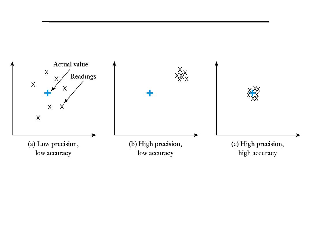
• Accuracy, inaccuracy, uncertainty:
accuracy
is a measure of the maximum expected error
• Sensitivity:
a measure of the change produced
at the output for a given change in the quantity
being measured
Some Definitions(Measuring
)
• Precision:
a measure of the lack of random
errors (scatter)
• Linearity:
maximum deviation from a
‘straight-line’ response, normally expressed as
a percentage of the full-scale value
A Real-Time System Model
Real-time
control system
Actuator
Actuator
Actuator
Actuator
Sensor
Sensor
Sensor
Sensor
Sensor
Sensor

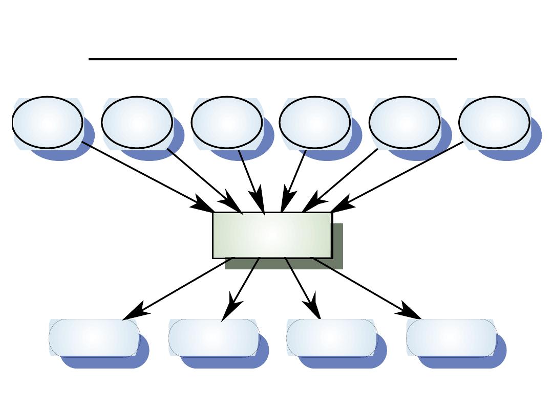
System Elements
• Sensors control processes
– Collect information from sensors. May
buffer information collected in response to a
sensor stimulus
• Data processor
– Carries out processing of collected
information and computes the system
response
• Actuator control
– Generates control signals for the actuator
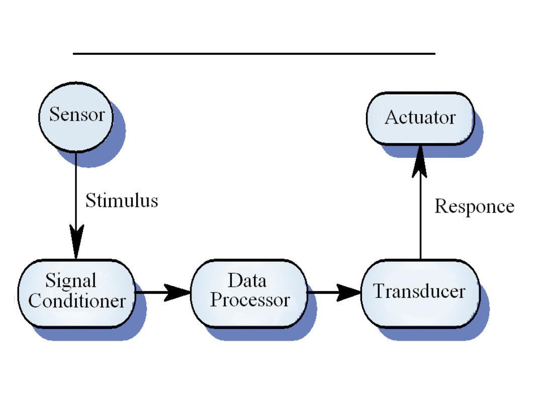
Sensor/Actuator Processes
Data
processor
Actuator
control
Actuator
Sensor
control
Sensor
Stimulus
Response

System Design
• Design both the hardware and the software
associated with the system. Partition
functions to either hardware or software
• Design decisions should be made on the
basis of non-functional system requirements
• Hardware delivers better performance but
potentially longer development and less
scope for change
• Good design Stand-alone components
that can be implemented in either software
or hardware
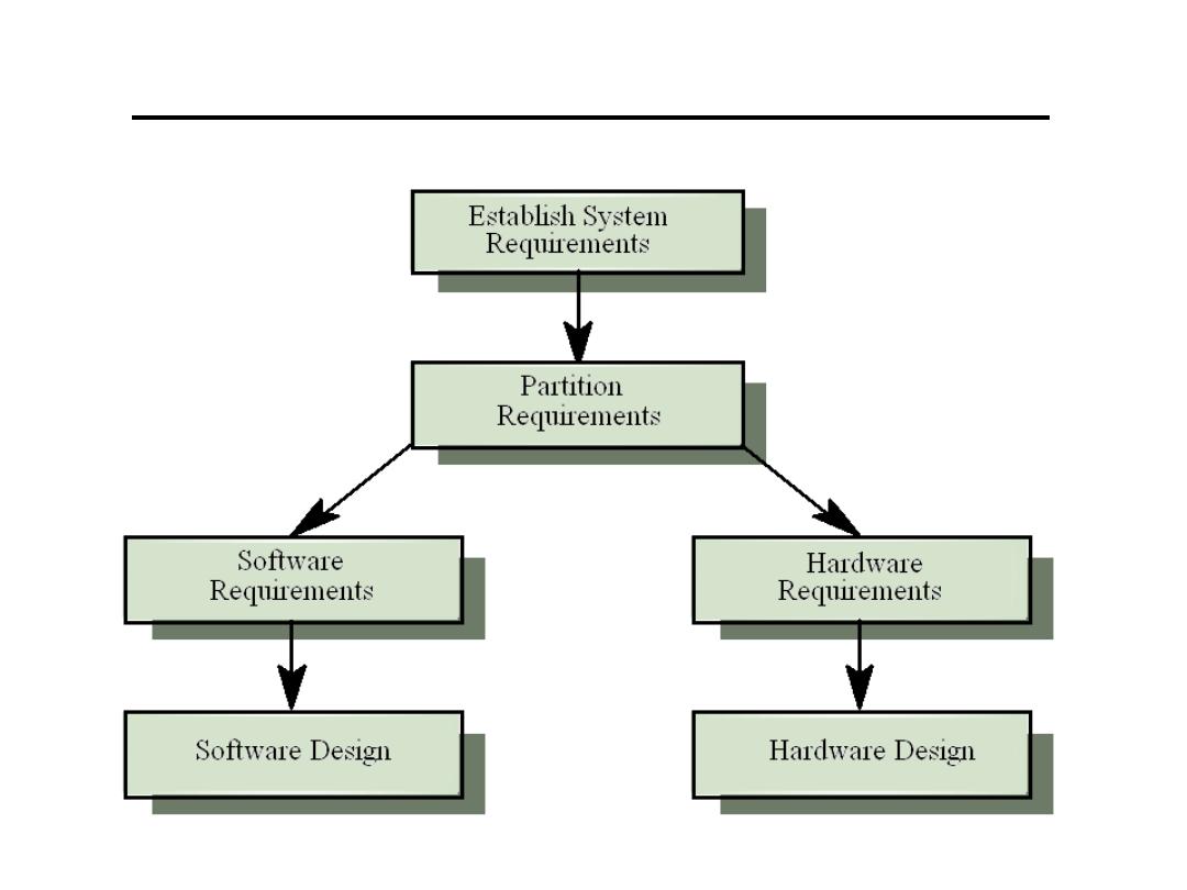
Hardware and Software Design

Sensors and There Classification
• Sensors and actuators are examples of
transducers
A transducer is a device that converts
one physical quantity into another
• Almost any physical property of a material that
changes in response to some excitation can be
used to produce a sensor
– widely used sensors include those that are:
1. Resistive 6. Elastic
2. Capacitive 7. Piezoelectric
3. Inductive 8. Photoelectric
4. Electromagnetic 9. Pyroelectric
5. Thermoelectric 10. Hall effect
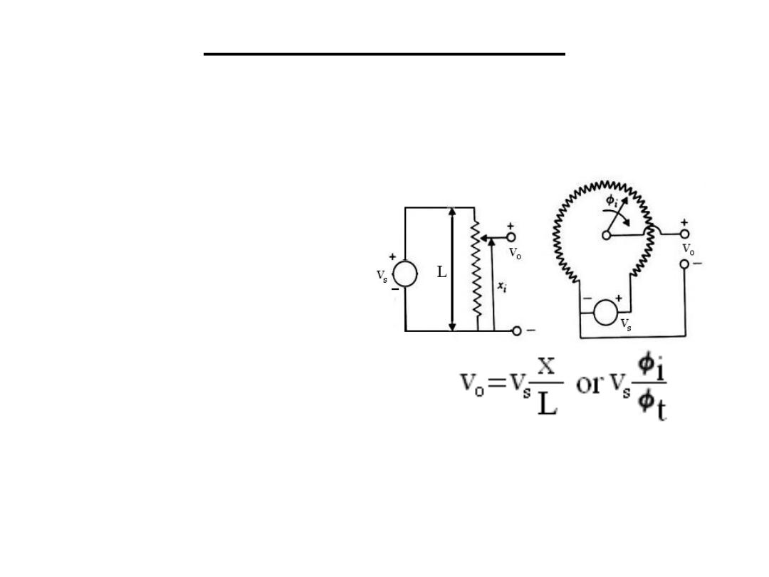
1.Resistive Sensors
1.1 Potentiometers: It is a resistance element
with a sliding contact which is moved over the
length of the element.
• Used for monitoring
Linear or circular
displacements.
• The fraction ratio (f ) is
equal to f = x/L =
φ
i/
φ
t
•If the total track resistance =Rp then the
resistance between the sliding terminal and the
reference terminal = f Rp
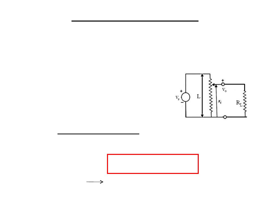
Potentiometers are linear elements (Vo is
linearly proportional to Vs) but as a load is
placed across the output linearity disappear and
error is introduced.
R
total=
f RpR
L
/ f Rp+R
L
Vo=Vs* Rtotal/ Rtotal+(1-f )Rp
=Vs f
a
(Rp/R
L
)f (1-f )+1
Error=f Vs – Vo = Vs(Rp/R
L
)(f
2
-f
3
)
d(error)/df =0 f =2/3 for max. error
1.Resistive Sensors

Ex: If a voltmeter of 10K
Ω
internal resistance is connected to a potentiometer of
500
Ω
total resistance which is connected to a 10V voltage source 1)find the error
if the slide is a)at the middle b)at the position for max. error. 2)who does reducing
the voltage of the source effect the error, what is its disadvantage suggest another
way to reduce the error
1.Resistive Sensors
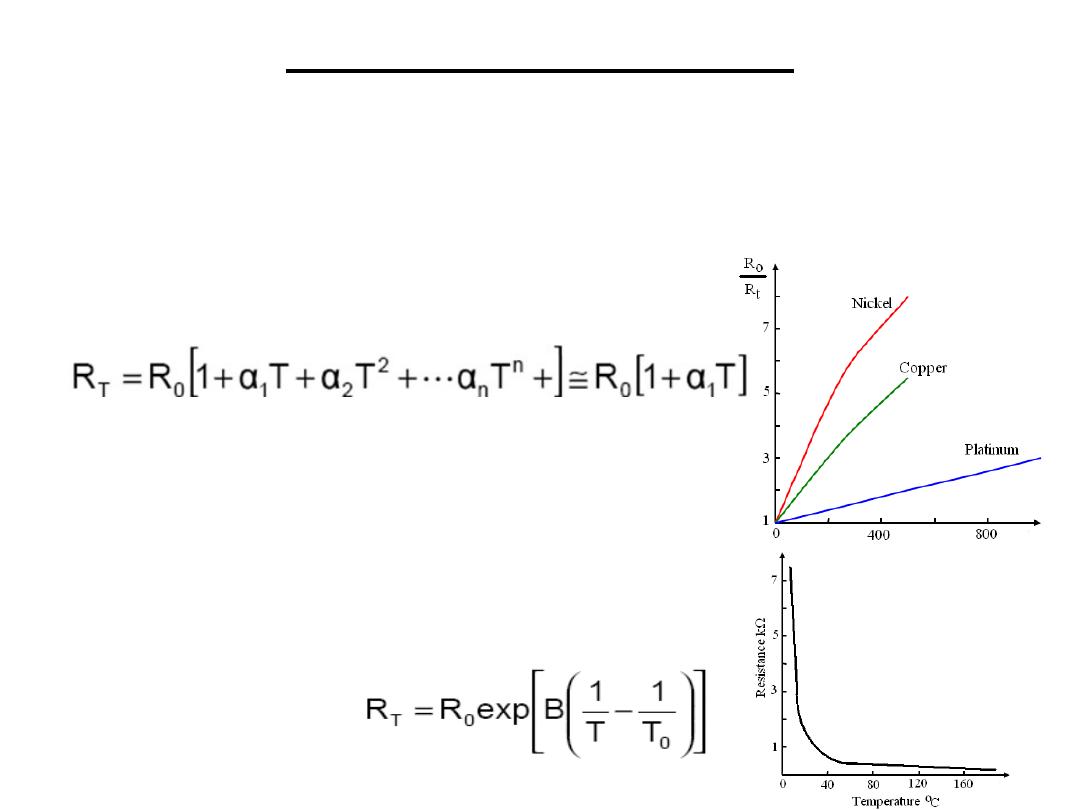
1.2 Resistance Temperature Devices (RTDs):
RTDs are made of materials whose resistance
changes in accordance with temperature
a)Metals
b)Metal oxides or
Semiconductors:
Generally, they
have a negative temperature
coefficient and an exponential
relationship
Cheep, fast (avalanche problem)
1.Resistive Sensors
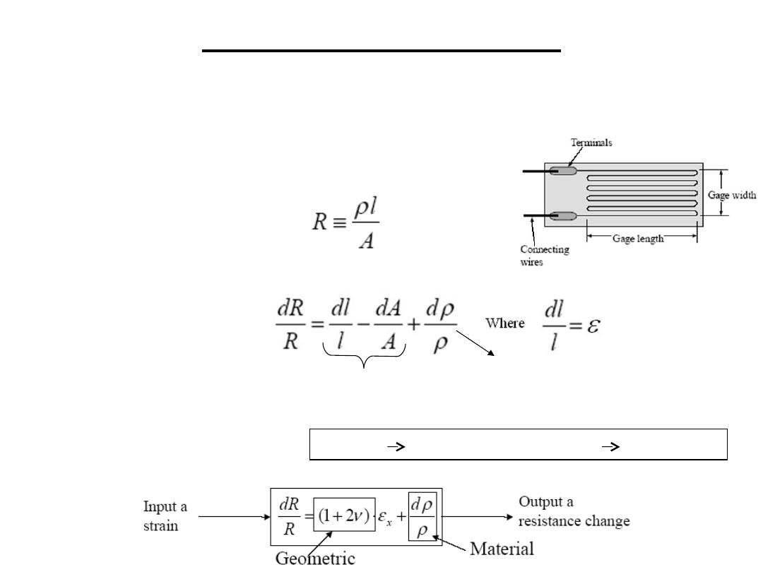
1.3 Strain Gauge: consists of a resistance element
in the form of a flat coil of wire
1.Resistive Sensors
Resistance is related to length and area of cross-section of the
resistor and resistivity of the material as
By taking logarithms and differentiating both sides, the equation becomes
Dimensional
piezoresistance
The strain
ε
is in the direction of stretching and is related to the transverse strain by poisson’s
ratio (v ) as :
transverse strain = - v
ε
A=
π
d
2
dA=2
π
d dd (
Α=
π
d
2
) dA/A=2dd/d
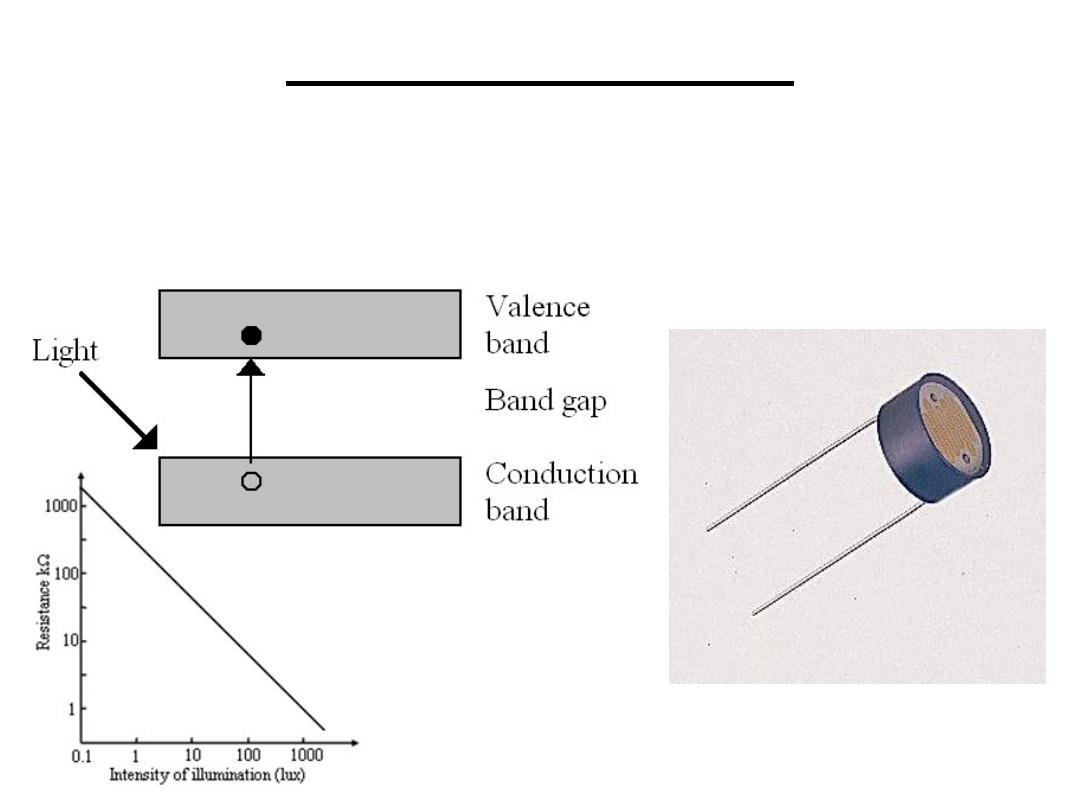
1.4 Photo conductive: semiconductors used for
their property of changing resistance when
electromagnetic radiation is incident on them.
1.Resistive Sensors
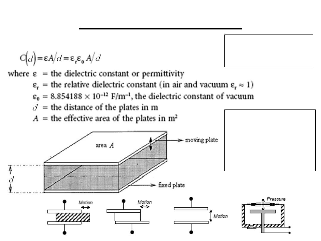
2.Capacitive Sensors
e.g. An electrolytic
capacitor is made of
Aluminum evaporated
on either side of a very
thin plastic film (or
electrolyte)
Electrolytic or ceramic
capacitors are most
common
The capacitance of a parallel plate capacitor is
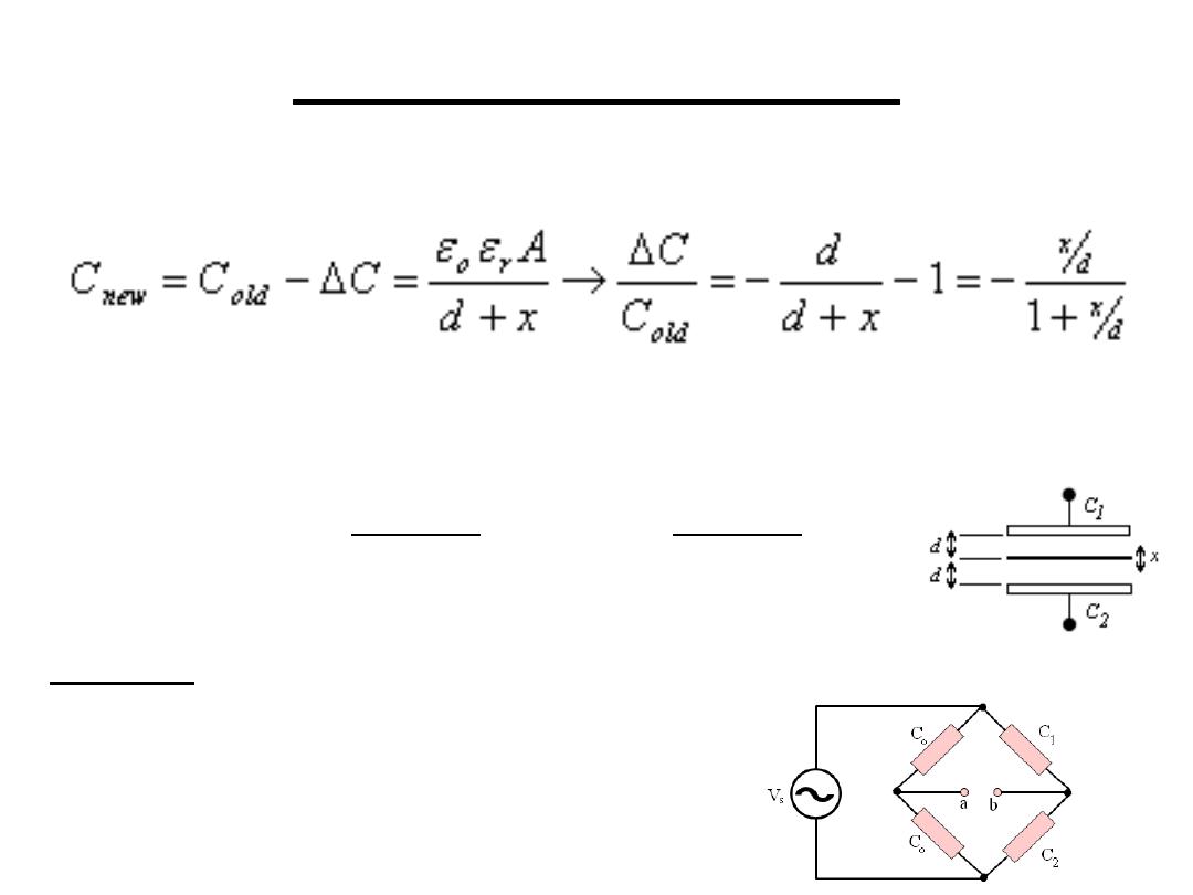
2.1 Displacement sensor: if the distance d is
increased by displacement x then:
This is a non-linear relationship and can be
overcome by using a push-pull displacement
sensor
H.W. if C1 & C2 are placed as shown find the
relation between Vab and x
2.Capacitive Sensors
x
d
A
andC
x
d
A
C
r
o
r
o
−
=
+
=
ε
ε
ε
ε
2
1
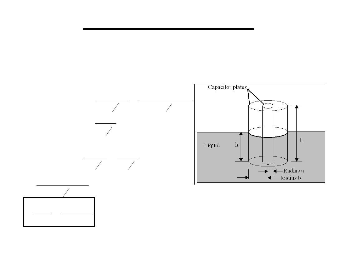
2.2 Liquid level sensor: the capacitor plates are a
rod surrounded by a concentric cylinder .
2.Capacitive Sensors
)
ln(
)
(
2
)
ln(
2
sensor
of
e
capacitanc
a
b
r
o
a
b
r
o
h
L
h
−
+
=
ε
π ε
ε
π ε
]
)
1
(
[
)
ln(
2
sensor
of
e
capacitanc
h
L
r
a
b
o
−
+
=
ε
π ε
L
h
h
h
L
L
r
a
b
r
o
r
a
b
o
a
b
o
)
1
(
C
C
So..
)
ln(
)
1
(
2
]
)
1
(
[
)
ln(
2
)
ln(
2
C
C
C
old
new
old
−
=
∆
−
=
−
+
−
=
−
=
∆
ε
ε
π ε
ε
π ε
π ε
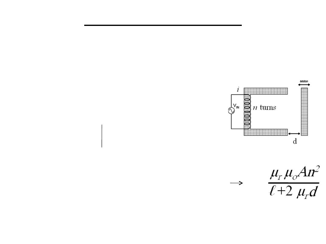
3.1 Variable reluctance sensor: in a similar way
that a electromotive force drives current through a
resistance a magneto motive force drives flux
though a reluctance
m.m.f=flux (
φ
)*reluctance(S)=n*i
Reluctance(S) =ℓ/ μ
r
μ
o
A
d=0
Reluctance of air gap (S
a
)=2d/ μ
o
A
S
T
= ℓ/ μ
r
μ
o
A+ 2d/ μ
o
A =ni/
φ
, L=n
φ
/ i L=
L depends on d .This is a non-linear relationship
and can be overcome by using a push-pull sensor
3.Inductive Sensors
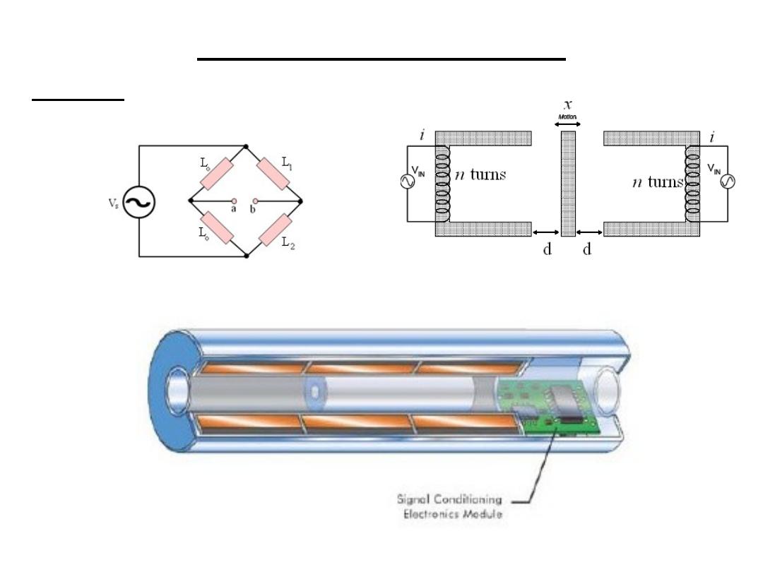
H.W. if L1 & L2 are placed as shown find the
relation between Vab and x
3.2 Linear variable reluctance sensor:
3.Inductive Sensors
LVDT
Linear Variable
Differential
Transformer
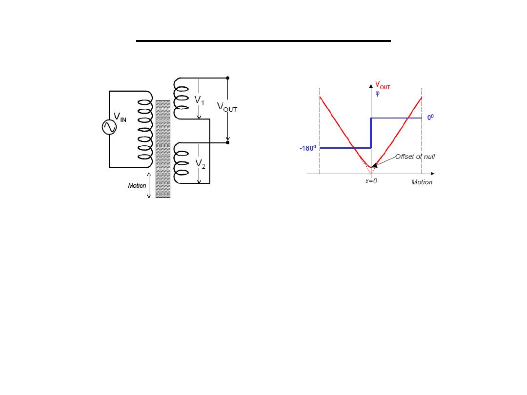
•Motion of a magnetic core changes the mutual inductance of two secondary coils
relative to a primary coil
•Primary coil voltage: V
S
sin(ωt)
•Secondary coil induced emf: V1=k1sin(ωt+ϕ) and V2=k2sin(ωt+ϕ)
•k1 and k2 depend on the amount of coupling between the primary and the
secondary coils, which is proportional to the position of the coil
• When the coil is in the central position, k1=k2 VOUT=V1-V2=0
⇒
• When the coil is displaced x units, k1≠k2 VOUT=(k1-k2)sin(ωt+ϕ)
⇒
• Positive or negative displacements are determined from the phase of VOUT
3.Inductive Sensors
Primary Secondary
Displacement Sensor
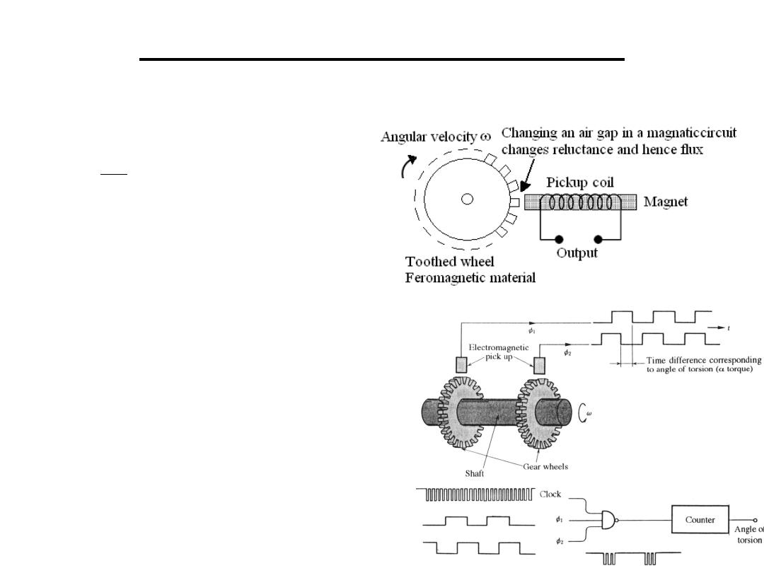
4.Electomagnatic Sensors
4.1Tachogenerator: used to measure angular
velocity
•An other way is to transform
the output to pulses which are
counted by a counter
•The use of an AC generator
is an other way to measure ω
t
n
n
N
e
t
n
n
N
e
t
n
dt
d
N
e
a
a
o
a
ω
ω
φ
ω
ω
φ
φ
ω
φ
φ
φ
sin
]
sin
[
teeth
No.of
where
cos
turns
No.of
where
=
−
−
=
+
=
−
=
n
N
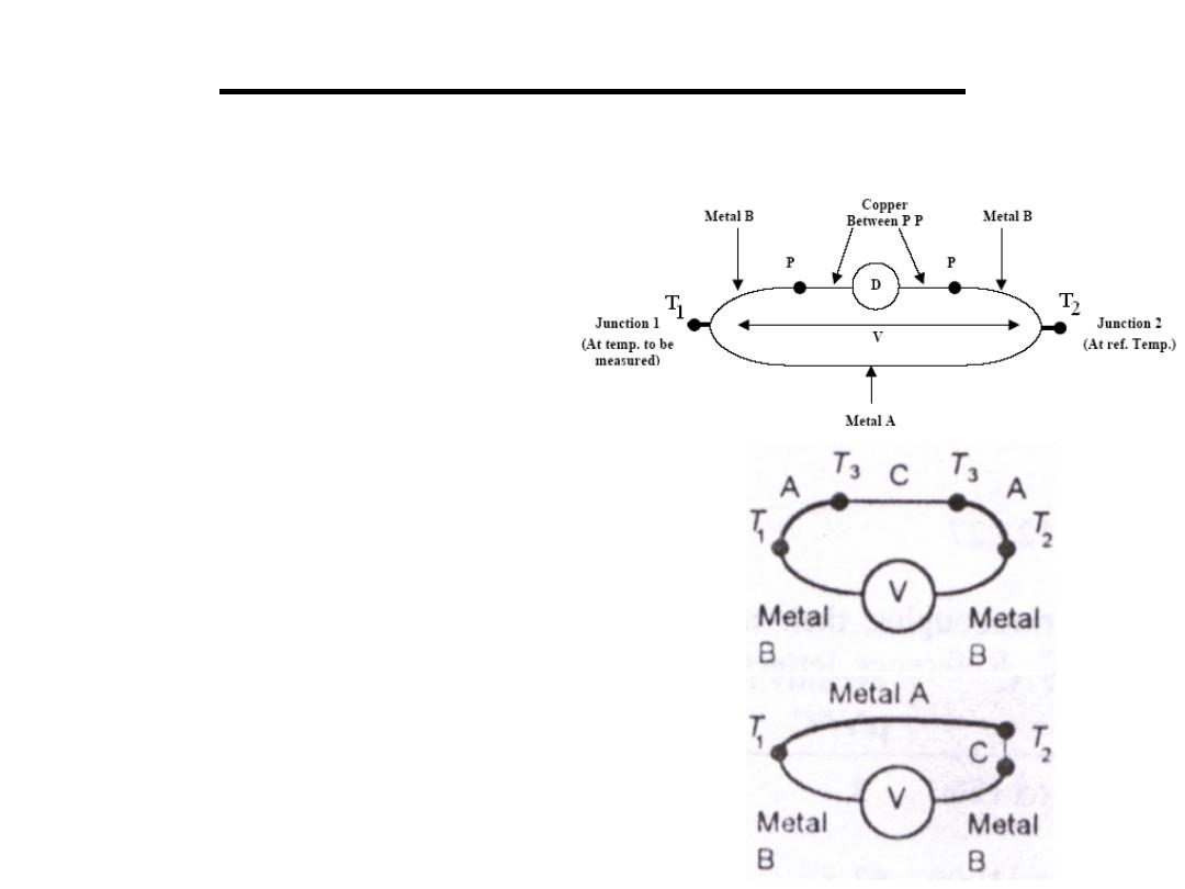
Thermocouple:
connecting two different metals produces a
potential difference across the junction
V α (T
1
– T
2
)
1.The e.m.f depends only on the
temperature of the junction
2.If a third metal C is added the e.m.f is
unchanged if the two new junctions are
at the same temperature.
3. If a third metal C is added at either
junctions the e.m.f is unchanged if the
two new junctions (AC ,CB) are at the
same temperature.
4. If the e.m.f produced at AC & CB is
E
AC
&E
CB
then E
AB
= E
AC
+ E
CB
.
5.Thermoelectric Sensors
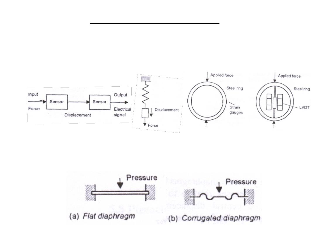
• Springs and load cells: used to transform
forces into displacements which can be
transformed to electric signals.
• Diaphragms: pressure difference between its
two sides results in displacement.
6.Elastic Sensors
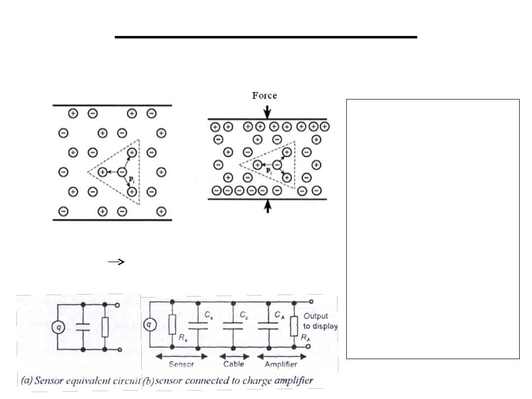
• Piezoelectricity: some dielectric materials
when stretched its surfaces become charged
7.Piezoelectric Sensors
Strain causes a
redistribution of charges
and results in a net
electric dipole (a dipole
is kind of a battery!)
A capacitor like
structure
A piezoelectric material
produces voltage by
distributing charge
(under mechanical
strain/stress)
q=kx =SF k,S are constants called charge sensitivity
C=q/V=ε
o
ε
r
A/d V=(Sd/ε
o
ε
r
A) F , pressure(P) = F/ A
V=S
v
dP ,S
v
= S/ε
o
ε
r
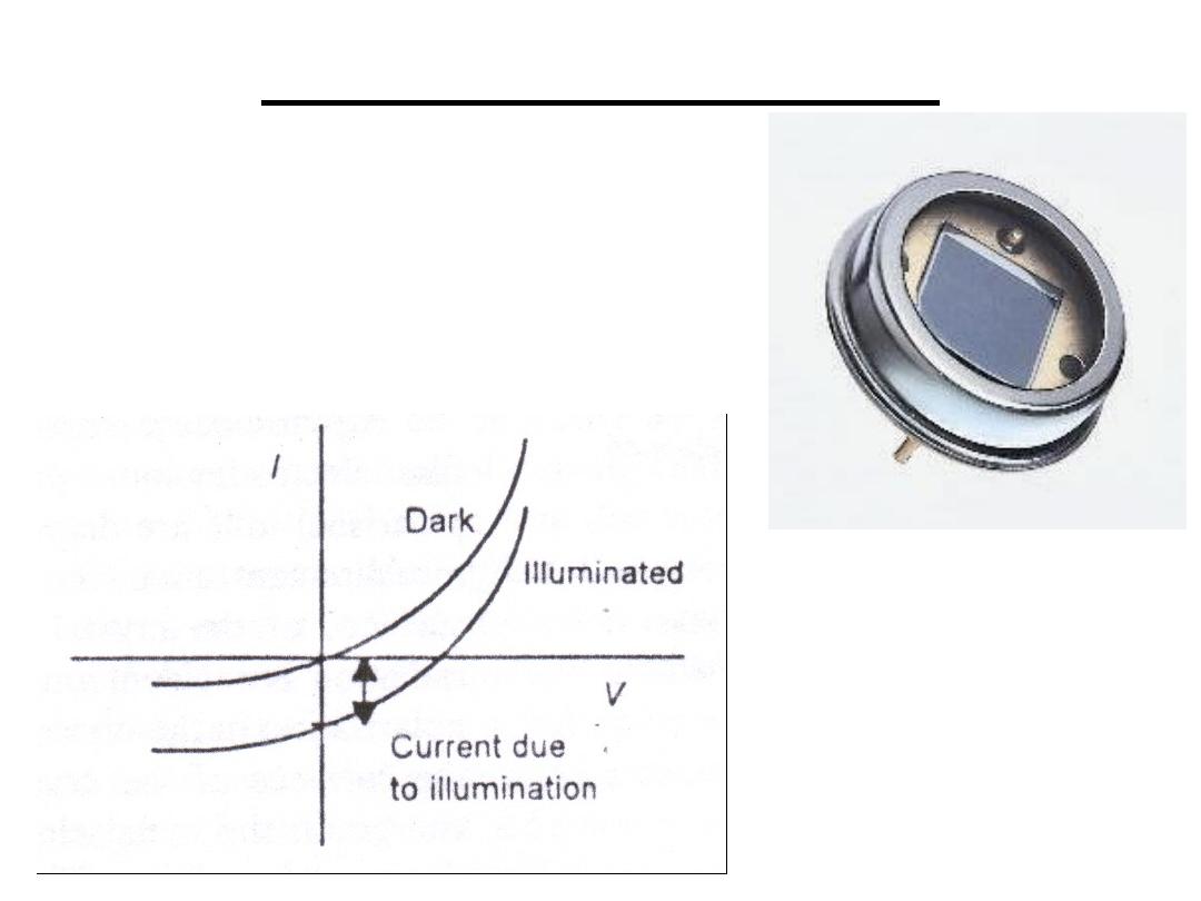
They are p-n junctions which
produce a change in current
when electromagnetic radiation
is incident on the junction.
8.Photovolatic Sensors
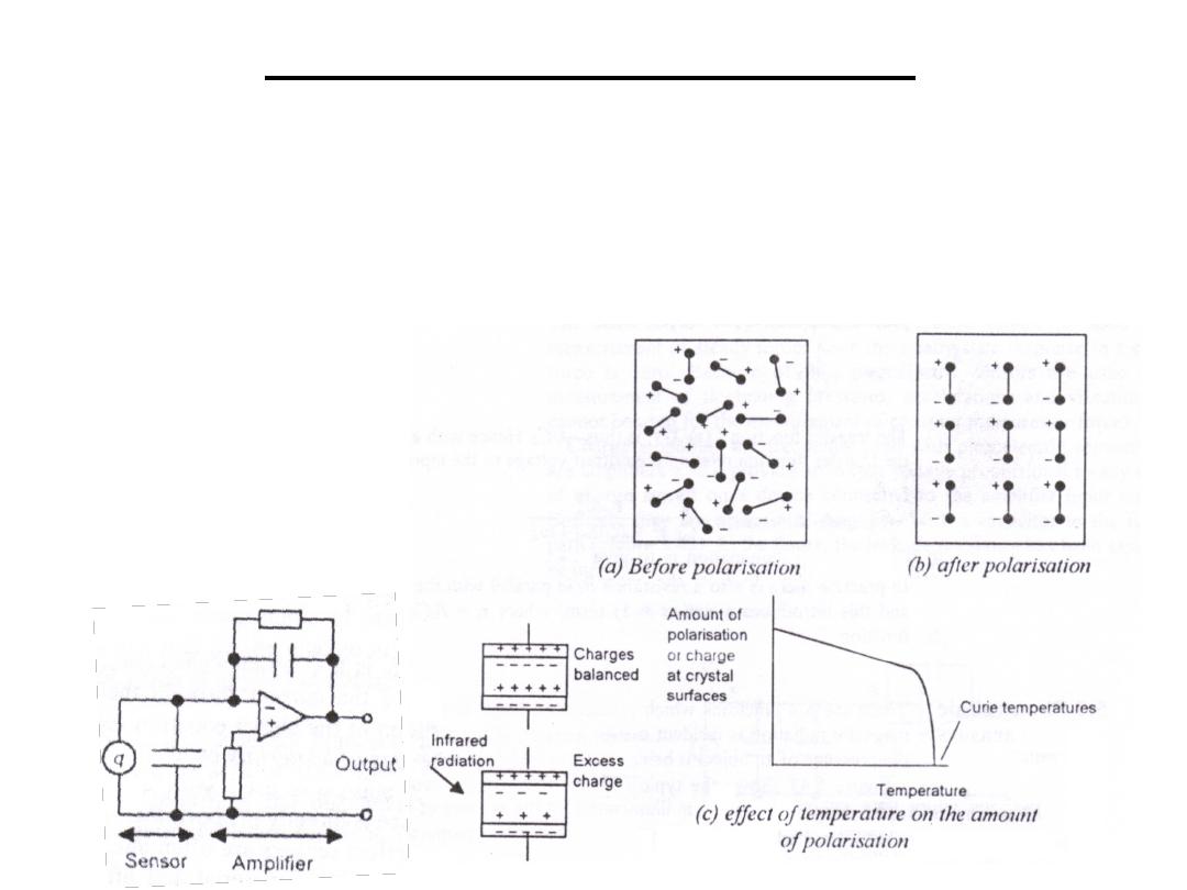
•Certain materials (lithium tantalate crystals) when an electric
field is applied across it at a temp. below the Curie temp. and
then cooled it becomes polarized as a result of electric dipoles
within it. When the pyroelectric material is exposed to infrared
radiation its temp. rises and the amount of polarization is
reduced.
•Used to measure sensitive
temperature changes.
•Charge decreases as temperature
increases.
9.Pyroelectric Sensors
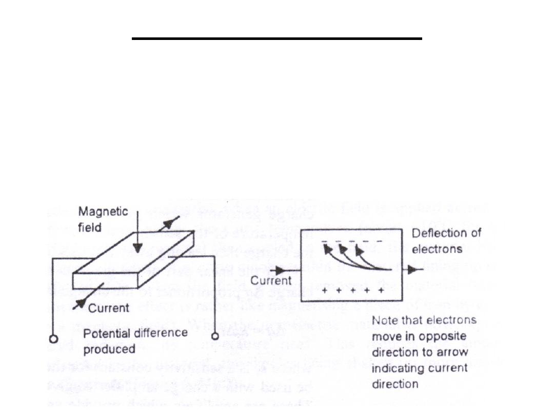
The action of a magnetic field on a flat plate
carrying an electric current generates a potential
difference which is a measure of the strength of
the field. A beam of charged particles can be
deflected by a magnetic field (Hall effect).
10.Halleffect Sensors

• Provide excitation source that transforms the
changes in electrical parameters to voltages
•Some functions of signal conditioners are:
1.Adjusting of the sensor signals
2.Conversion of currents to voltages
3.Supply of (ac or dc) excitations to the sensors
so changes in resistance, inductance, or
capacitance are converted to changes in voltage
4.Filtering to eliminate noise or other unwanted
signal components
5.Making a nonlinear signal a linear one
Signal Conditioning
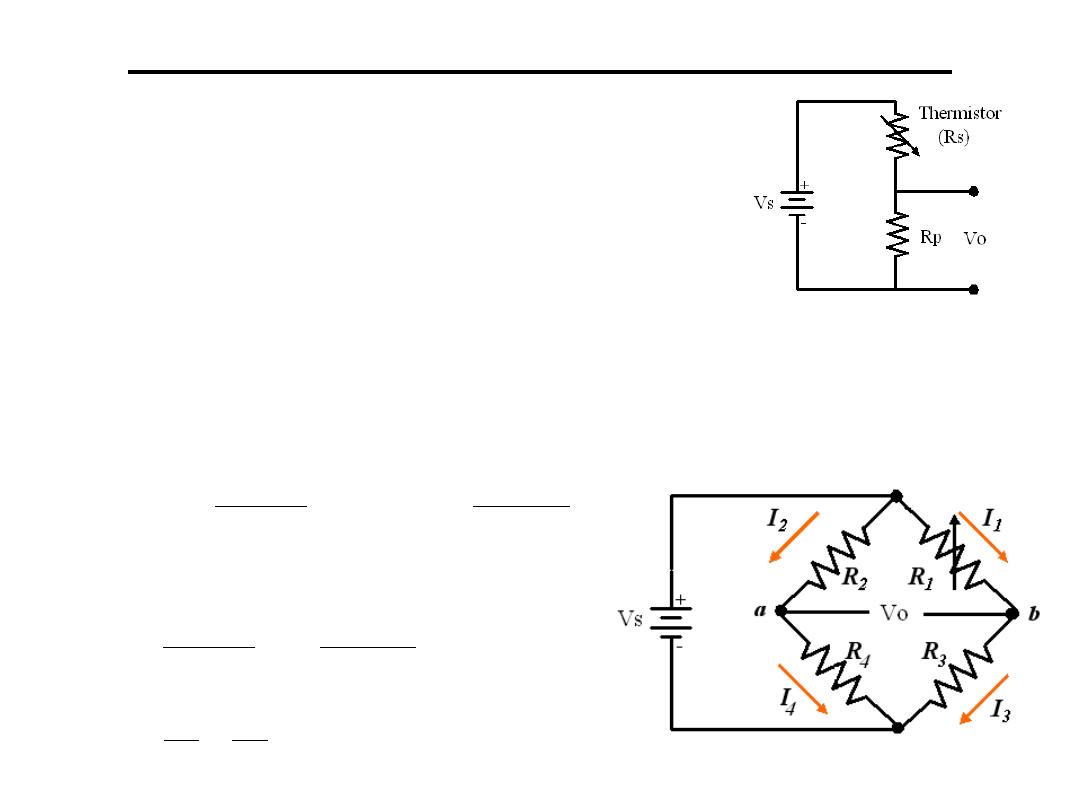
1.Potentiometer: used to transfer
changes in resistance (Thermistor
or strain gauge) to voltage
Vo=Vs*Rp/(Rp+Rs)
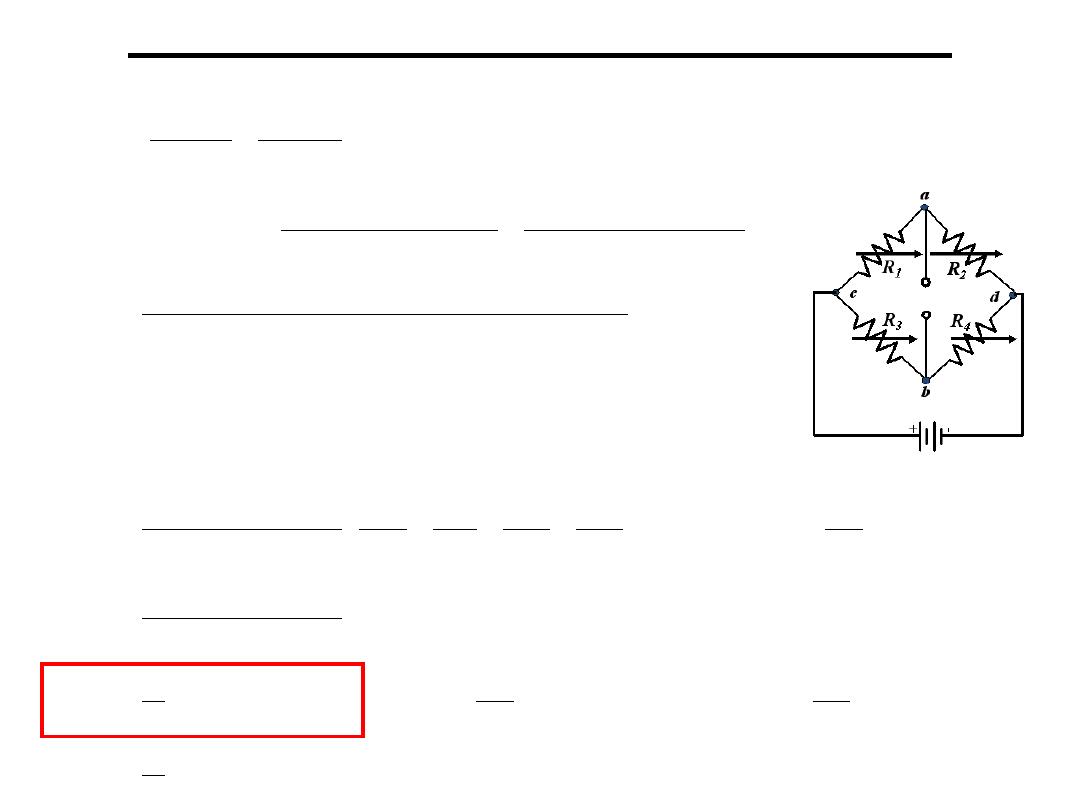
2.Wheatstone bridge: Consists of 4 resistors in
a diamond orientation, with a resistive
transducer in one or more legs.
Resistance to Voltage Conversion
0
,
if
4
2
3
1
4
2
2
3
1
1
2
2
1
1
4
2
4
2
3
1
3
1
=
=
+
−
+
=
−
=
+
=
=
+
=
=
o
S
S
o
o
S
S
V
R
R
R
R
V
R
R
R
V
R
R
R
V
R
I
R
I
V
R
R
V
I
I
R
R
V
I
I
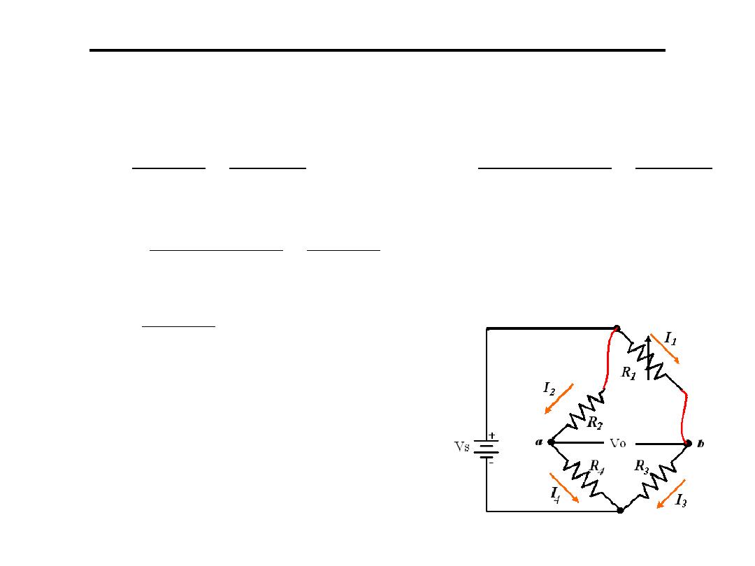
If R1 is a sensor its resistance is changed to be
R1+ΔR1 therefore Vo is changed to Vo+ΔVo
The resistance of wires connecting R1
will be effected by temp. so the
connection shown is used so the
effect of temp. is added to the two
opposite branches
Resistance to Voltage Conversion
3
1
1
1
1
3
1
1
3
1
1
1
1
4
2
2
3
1
1
1
1
4
2
2
3
1
1
if
,
R
R
R
V
V
R
R
R
R
R
R
R
R
R
R
V
V
R
R
R
R
R
R
R
R
V
V
V
R
R
R
R
R
R
V
V
S
o
S
o
S
o
o
S
o
+
∆
≈
∆
∆
> >
+
−
+
∆
+
∆
+
=
∆
+
−
+
∆
+
∆
+
=
∆
+
+
−
+
=
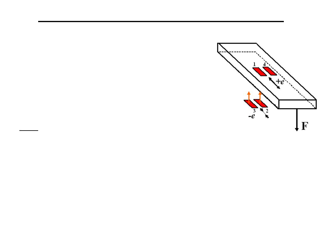
3.Temperature compensation with strain gauge
:
Strain gages are widely used in many
engineering measurement practices.
It often uses bridge circuit as its
conditioning circuit.
Ex: When 4 strain gages are used to measure
the force applied on free end of this cantilever, try to
1)Design bridge circuit for signal conditioning?
2)How about if only 2 strain gages are used?
Resistance to Voltage Conversion
3.Temperature compensation with strain gauge
:
Resistance to Voltage Conversion
[
]
[
]
)
1
(
2
n
compressio
for
and
strain
for
4
since
,
)
)(
(
gauge
strain
for
)
)(
(
terms
of
products
the
neglecting
and
have
We
)
)(
(
)
)(
(
)
)(
(
strain
after
3
2
4
1
4
3
2
1
4
3
2
1
2
2
3
3
1
1
4
4
4
3
2
1
4
1
2
2
3
3
1
1
4
4
4
3
2
1
4
1
3
2
4
1
4
3
2
1
3
3
2
2
4
4
1
1
4
4
3
3
3
3
2
2
1
1
1
1
4
3
3
2
1
1
neglected
be
can
and
ant
insignific
is
s,
resistance
of
sum
the
have
we
where
r term,
denominato
the
o
relation t
in
resistance
in
changes
The
v
G
V
V
Gv
R
R
G
R
R
G
V
V
G
G
G
G
R
R
R
R
G
G
G
G
R
R
R
R
R
R
V
V
G
R
R
R
R
R
R
R
R
R
R
R
R
R
R
R
R
V
V
R
R
R
R
R
R
R
R
R
R
R
R
R
R
R
R
V
V
R
R
R
R
R
R
R
R
R
R
R
R
V
V
R
R
R
R
R
R
V
V
S
o
S
o
S
o
S
o
S
o
S
o
S
o
+
=
−
=
∆
=
∆
−
−
+
=
=
=
=
=
=
=
−
−
+
+
+
=
=
∆
∆
−
∆
−
∆
+
∆
+
+
=
∆
=
+
+
∆
+
∆
+
−
∆
+
∆
+
=
∆
+
+
∆
+
∆
+
−
∆
+
+
∆
+
∆
+
=
+
−
+
=
ε
ε
ε
ε
ε
ε
ε
ε
ε
ε
ε
ε
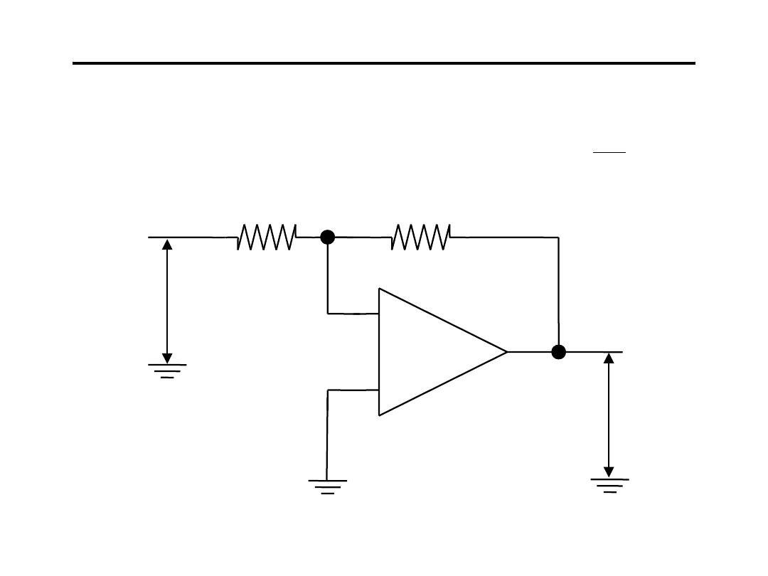
Operational Amplifier for Signal Conditioning
1. Inverting Amplifier:
+
-
R
1
R
2
V
o
-
+
-
+
V
i
i
1
2
0
V
R
R
V
−
=
Operational Amplifier for Signal Conditioning
2. Non-Inverting Amplifier:
R
1
+
-
-
+
R
2
V
o
V
i
-
+
i
1
2
o
V
R
R
1
V
+
=
Operational Amplifier for Signal Conditioning
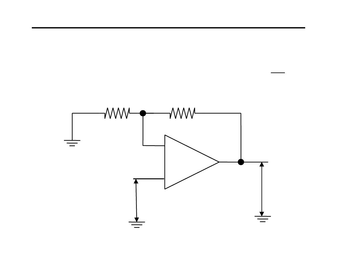
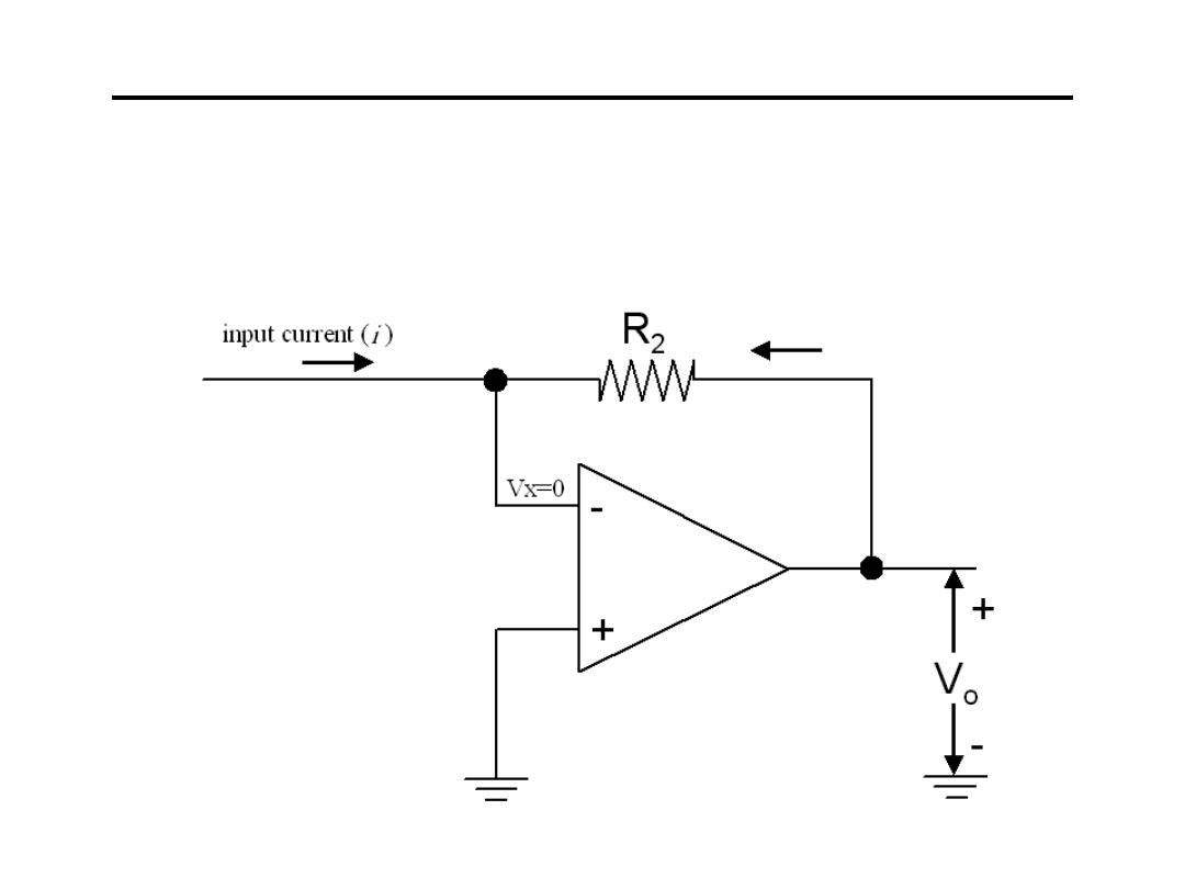
3.Current to Voltage Converter:
2
o
R
V
i
−
=
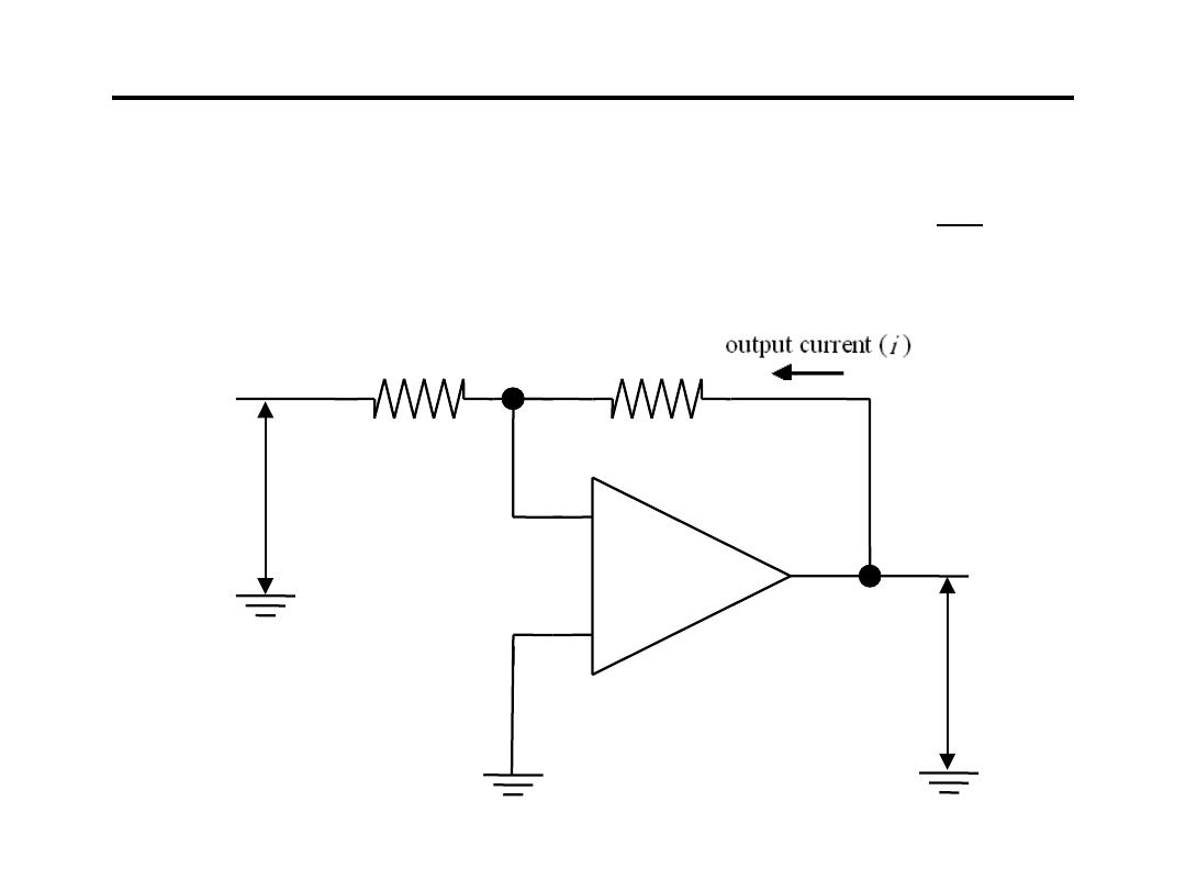
Operational Amplifier for Signal Conditioning
4.Voltage to Current Converter:
1
i
R
V
−
=
i
+
-
R
1
R
2
V
o
-
+
-
+
V
i
Operational Amplifier for Signal Conditioning
5.Summing Amplifier:
R
2
-
-
+
+
R
1
+
-
-
+
R
3
V
o
V
1
V
2
+
−
=
2
2
3
1
1
3
o
V
R
R
V
R
R
V
Operational Amplifier for Signal Conditioning
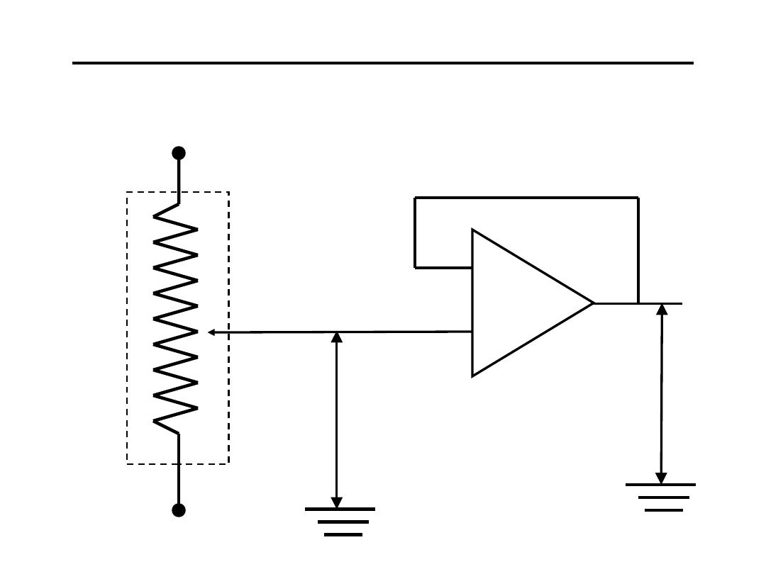
6.Voltage Divider “Buffered” :
+12V
-12V to +12V
-
+
-
+
-12V to +12V
-
+
-12V
Operational Amplifier for Signal Conditioning
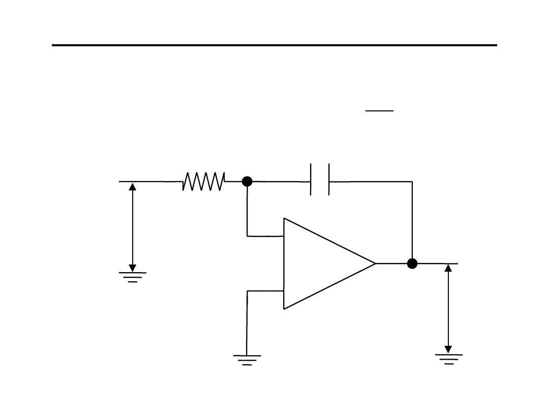
7.Integrating Amplifier:
+
-
R
V
o
-
+
-
+
V
i
C
∫
+
−
=
t
0
o
i
o
(0)
V
dt
V
RC
1
V
Operational Amplifier for Signal Conditioning
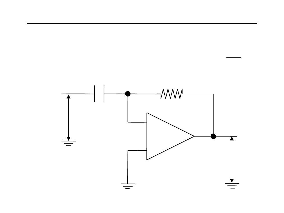
8.Differentiating Amplifier:
+
-
R
V
o
-
+
-
+
V
i
C
dt
dV
i
RC
V
o
−
=
Operational Amplifier for Signal Conditioning
9.Comparator
-
-
+
+
+
-
-
+
<
−
>
+
=
ref
i
ref
i
o
V
V
if
12V
V
V
if
12V
V
V
o
V
ref
V
i
+12V
-12V
Operational Amplifier for Signal Conditioning
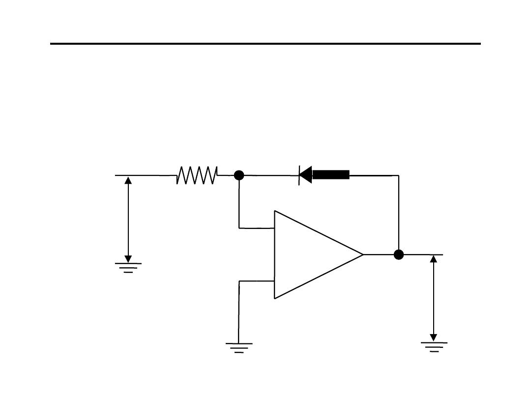
10.Logarithmic Amplifier :
(
)
R
C
/
V
ln
V
in
o
−
=
+
-
R
V
o
-
+
-
+
V
i
Operational Amplifier for Signal Conditioning
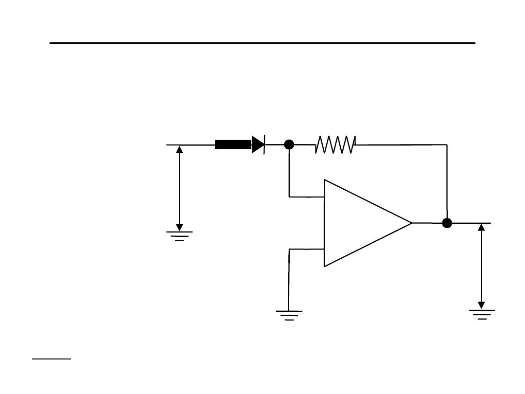
11.Anti-Logarithmic Amplifier :
HW: suggest a circuit that performs V
o
αV
1
*V
2
i
kV
e
V
o
α
+
-
R
V
o
-
+
-
+
V
i
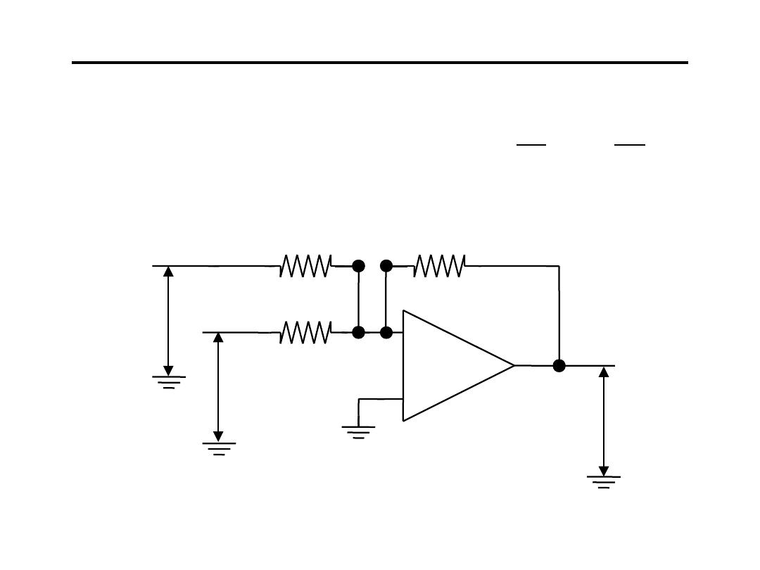
Operational Amplifier for Signal Conditioning
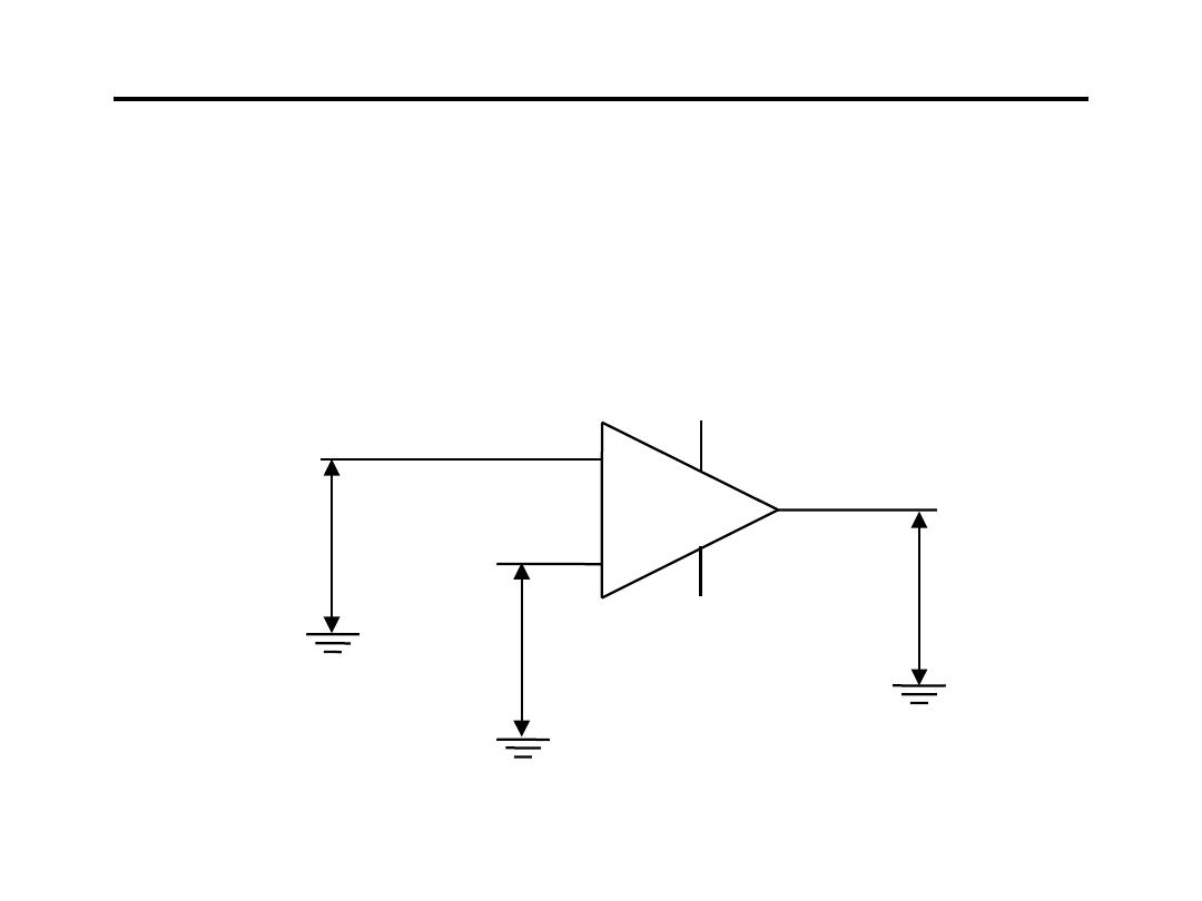
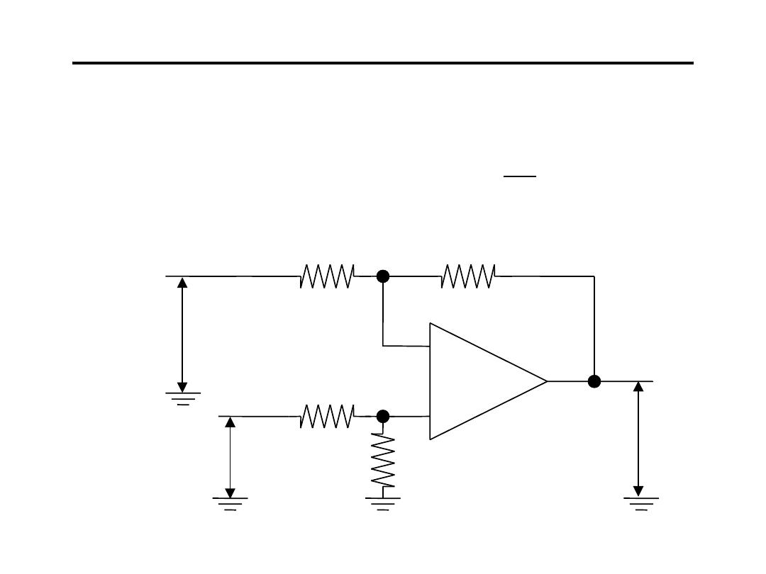
12. Difference Amplifier :
(
)
1
2
1
2
o
V
V
R
R
V
−
=
-
+
+
R
2
-
-
+
-
+
V
o
V
2
V
1
R
1
R
2
R
1
Operational Amplifier for Signal Conditioning
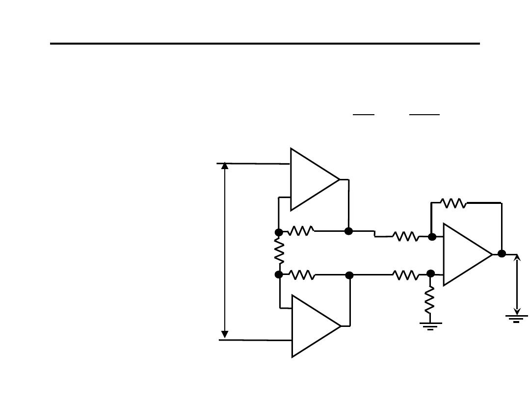
13.Instrument Amplifier :
• Low Input Current
• Low Drift
• Low Offset
• Stable & Accurate
• Three Amplifier-
Configuration
• High CMRR
-
+
+
-
-
+
-
+
R
G
i
3
1
2
o
V
2
1
V
+
=
G
R
R
R
R
R
3
R
2
R
1
R
3
R
2
R
1
V
o
-
+
V
1
Operational Amplifier for Signal Conditioning
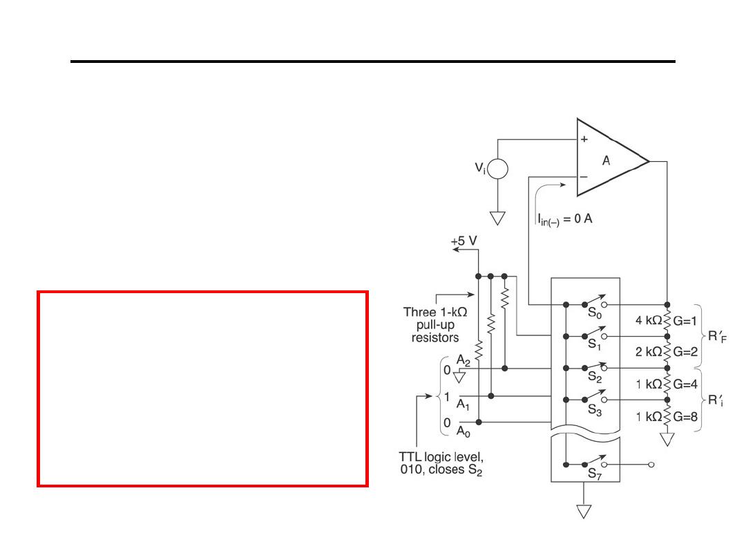
14.Programmable Gain Amplifier
•Non-Inverting Op Amps
•Digitally Controlled
•Addressable Inputs
HW: Drive the
relationship between
V
o
and V
i
for all of the
above Op-Amp.
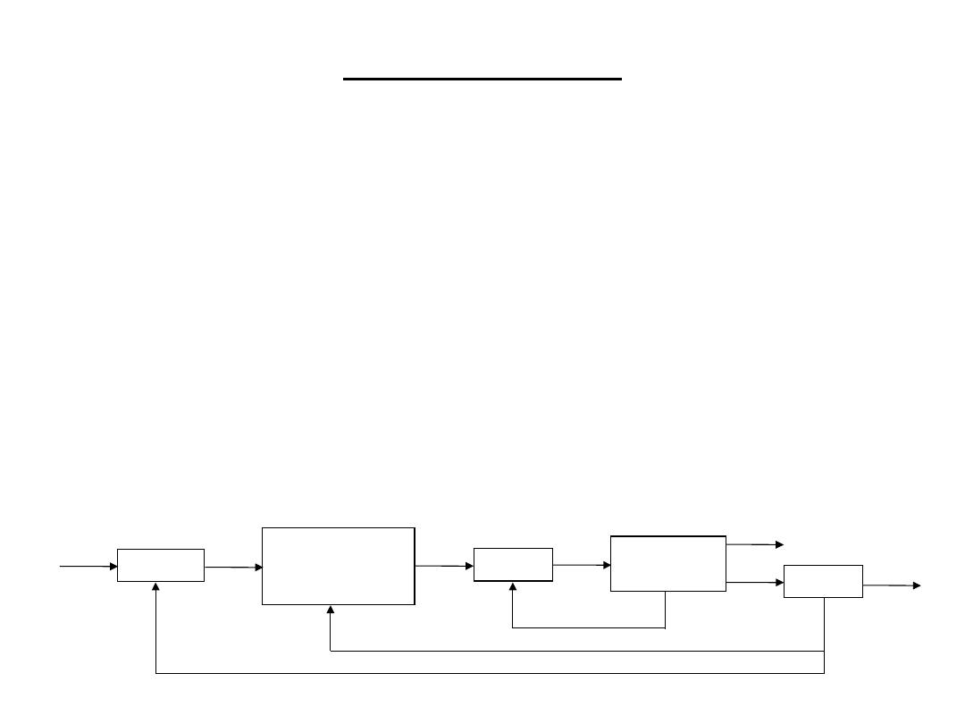
Smart Sensors
• Smart sensors are sensors that:
– Already put out signals that are in the right range.
– Have their own onboard or on-chip signal
conditioning circuit.
– Have error correction circuitry.
• They are expensive!
• Thus, it is important to be able to design signal
conditioning circuit for low cost sensors.
Sensor
Signal
Conditioning
Circuit
ADC
Micro-
processor
DAC
Digital output
Analogue
output
Control of ADC
Control of Signal Conditioning
Control over sensor
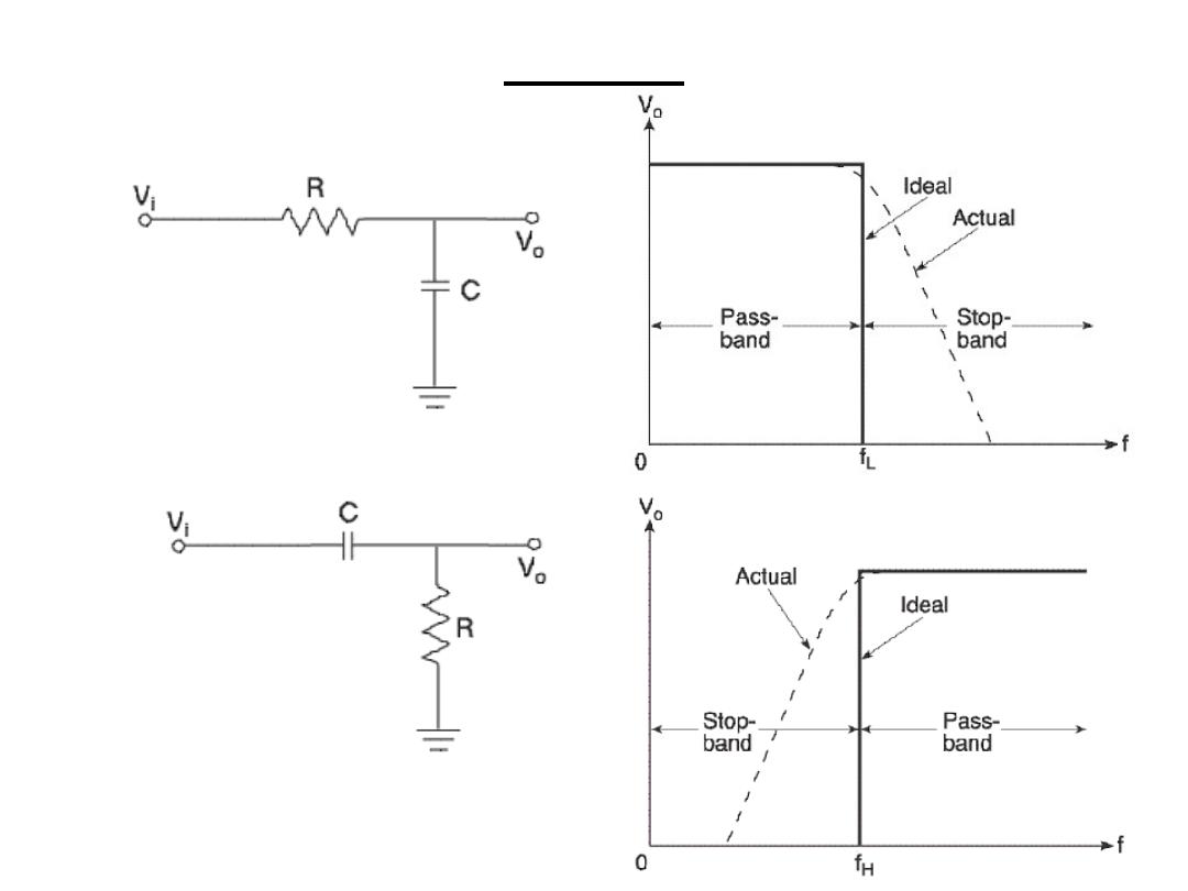
Filters
1.Low pass filter:
2.High pass filter
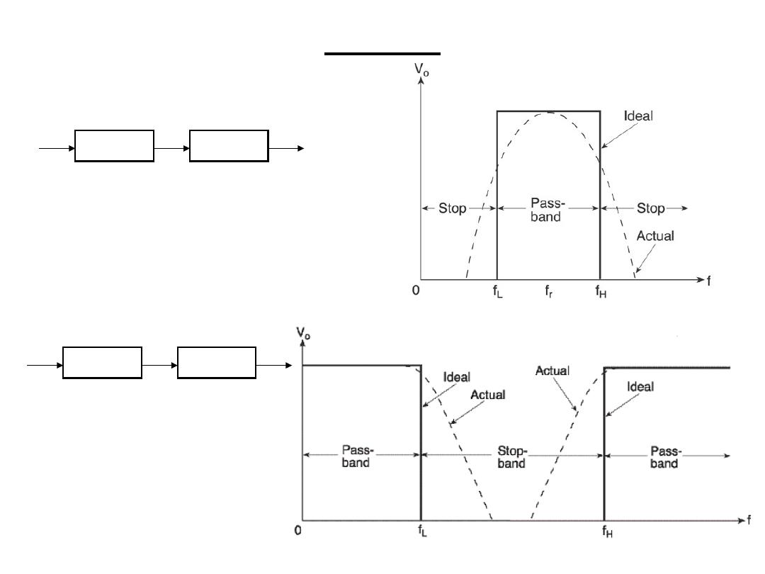
Filters
3.Band pass filter
:
f
L
> f
H
BW=
f
H
- f
L
4.Band reject filter
f
L
< f
H
RBW=
f
H
-
f
L
LPF
HPF
LPF
HPF
Digital to Analogue Converter
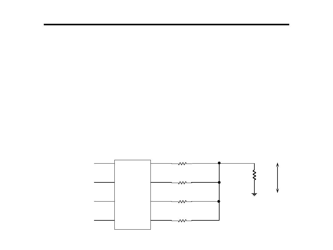
1.Weighted Registers D/A:
•Comprises of a register and resistor network
•Output of each bit of the register will depend on whether a ‘1’
or a ‘0’ is stored in that position
–for a ‘0’ then 0V output
–for a ‘1’ then 5V output
•Resistance R is inversely proportional to binary weight of
each digit
MSB
LSB
2R
4R
8R
R
L
V
L
4
-
bit
register
R
Digital to Analogue Converter
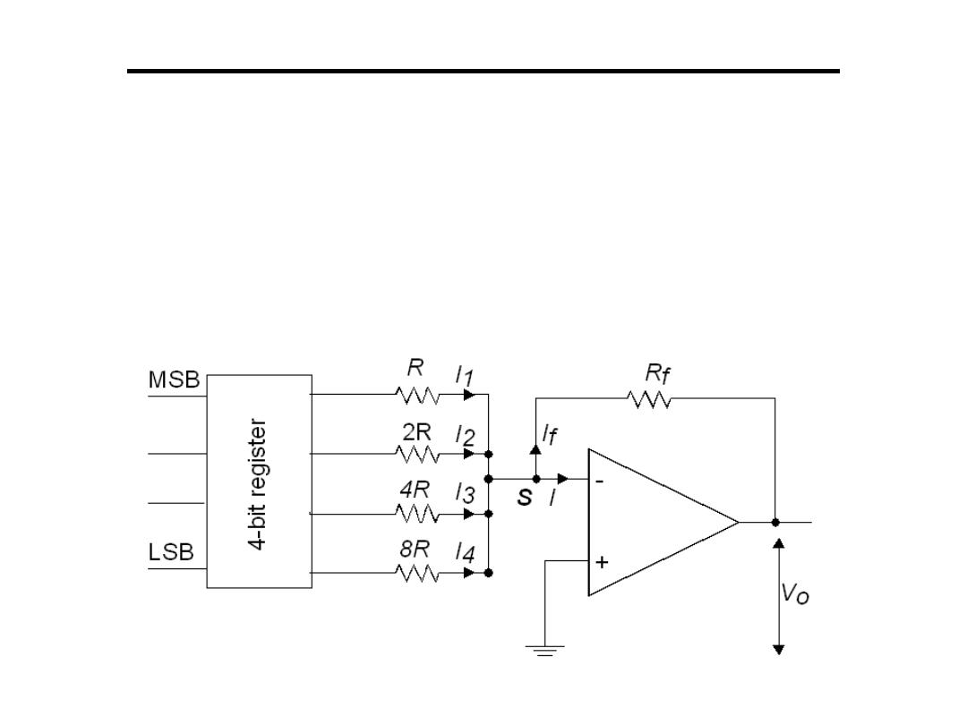
1.Weighted Registers D/A:
• Best solution is to follow the resistor network with a buffer
amplifier
–Has high impedance, practically no current flows
–All input currents sum at S and go through R
f
–V
o
= -I
f
R
f
V
o
= −
I
f
×
R
f
= −
)I
1
+
I
2
+
I
3
+
I
4
(
×
R
f

Digital to Analogue Converter
1.Weighted Registers D/A:
• Rarely used when more than 6 bits in the code word
• To illustrate the problem consider the design of an 8-
bit DAC if the smallest resistor has resistance R
– what would be the value of the largest resistor?
– what would be the tolerance of the smallest
resistor?
• Very difficult to manufacture very accurate resistors
over this range
Digital to Analogue Converter
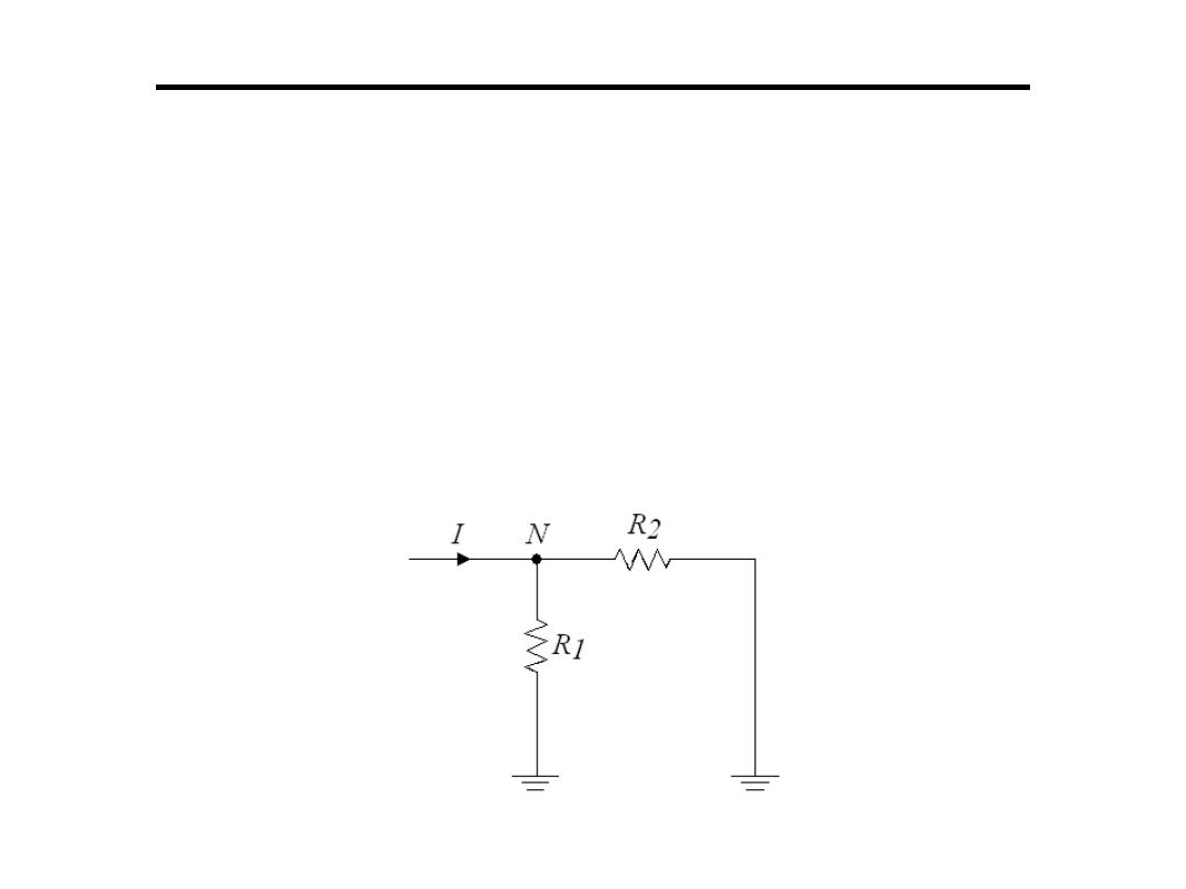
2.The R-2R Ladder:
•Has a resistor network which requires resistance values that
differ 2:1 for any sized code word
•The principle of the network is based on Kirchhoff's current
rule
•The current entering N must leave by way of the two resistors
R1 and R2
Digital to Analogue Converter
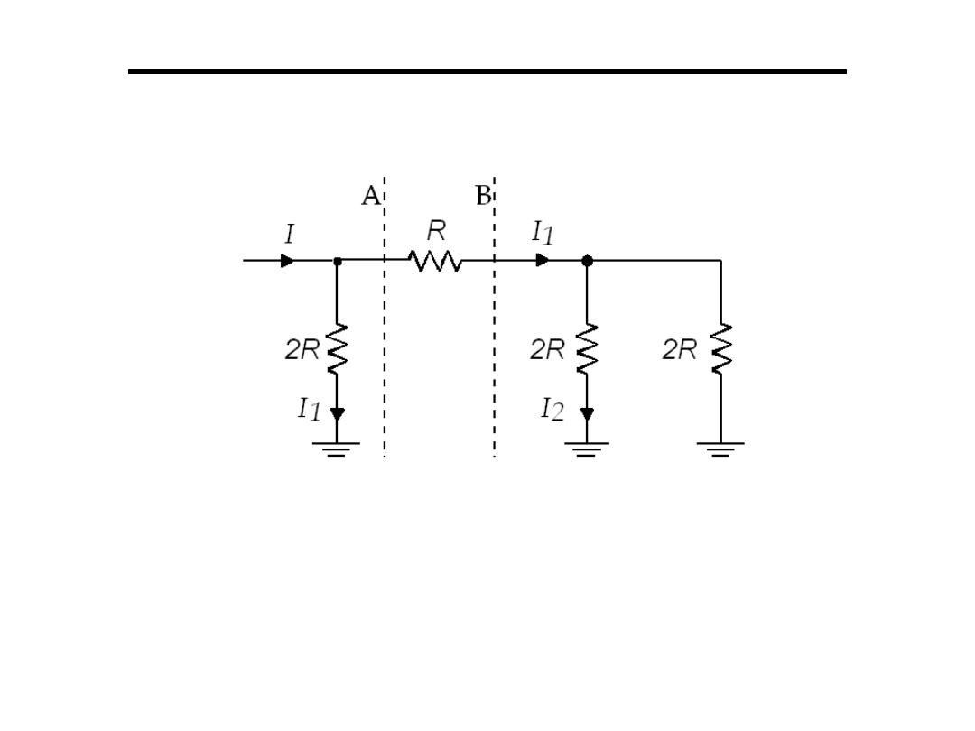
2.The R-2R Ladder:
– Works on a current dividing network
– Resistance to right of B = 1/(1/2R + 1/2R)
– Resistance to right of A = R +2R/2 = 2R
– Current divides I1 = I/2 , I2 = I/4 divides again
– The network of resistors to the right of A have an
equivalent resistance of 2R, and so the right hand
resistance can be replaced by a copy of the network
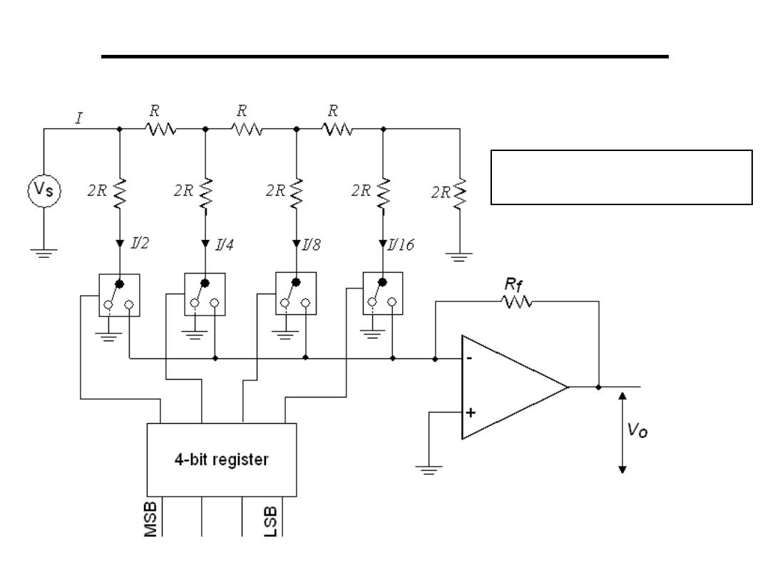
Digital to Analogue Converter
2.The R-2R Ladder:
The state of the bits is used
to switch a voltage source
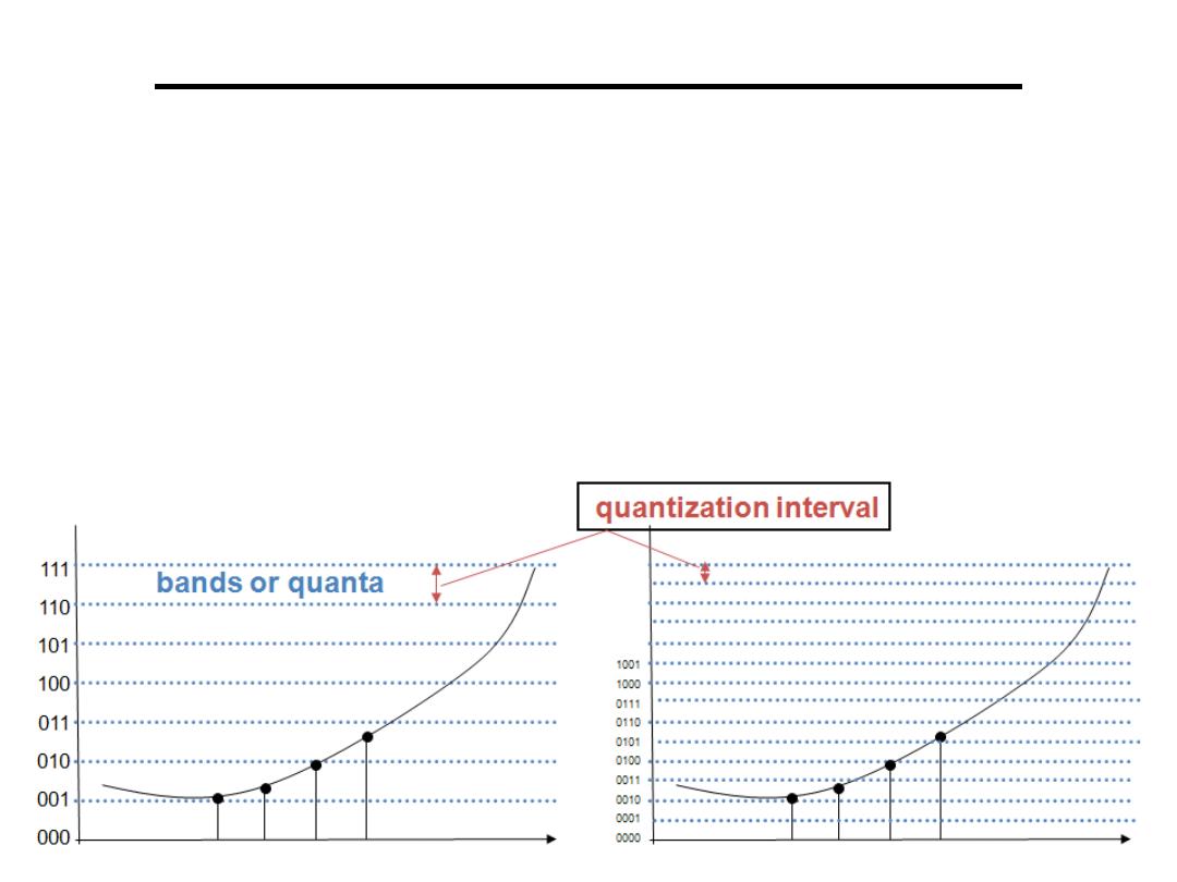
Digital to Analogue Converter
3.Quantization Error:
•Difference between the two waveforms is the quantization error
•Maximum quantization error is equal to half the quantization
interval
•One way to reduce the quantization error (noise) is to increase
the number of bits used by the D/A converter
•The voltage produced by the D/A convertor can be regarded as
the original signal plus noise
samples
samples
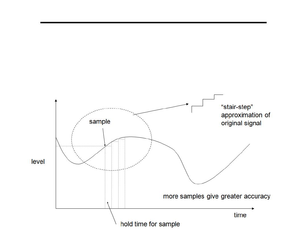
Analogue to Digital Converter
• A digital signal is an approximation of an
analog one
• Levels of signal are sampled and converted to
a discrete bit pattern.
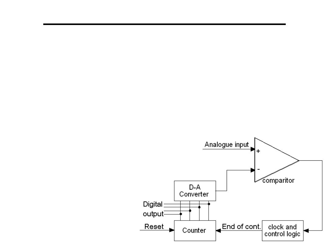
Analogue to Digital Converter
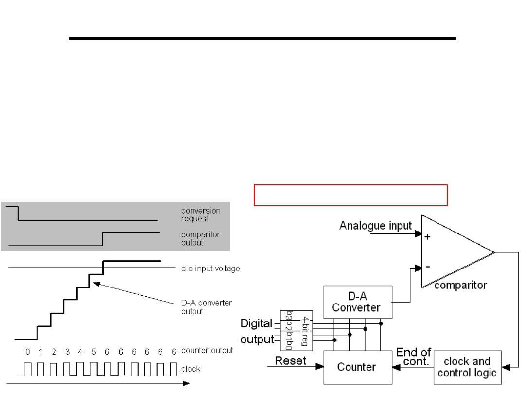
1.Stair Case or Counter-ramp:
– Comprises a D-A converter, a single comparator, a counter, a
clock and control logic
– When a conversion is required
• A signal (conversion request) is sent to the converter and the
counter is reset to zero
• A clock signal increments the counter until the reference
voltage generated by the D-A converter is greater than
the analogue input
• At this point in time the output of
the comparator goes to a
logic 1, which notifies the
control logic the conversion
has finished
• The value of the counter
is output as the digital
value
Analogue to Digital Converter
1.Stair Case or Counter-ramp:
– The time between the start and end of the conversion is known
as the conversion time
– A drawback of the counter-ramp converter is the length of time
required to convert large voltages
– We must assume the worst case when calculating conversion
times
HW: Find the conversation time
Analogue to Digital Converter
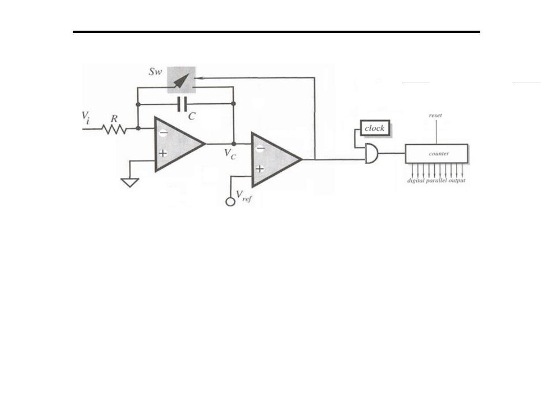
2.Voltage to Frequency Converter:
• These voltage-to-frequency converters or voltage controlled
oscillators are relatively simple and accurate circuits and have
been used for other purposes.
• The voltage across the capacitor is the integral of the current in
the noninverting leg of the amplifier.
• This current is proportional to the voltage across R.
• As the voltage on the capacitor rises, a threshold circuit checks
this voltage.
RC
t
V
dt
V
RC
1
V
i
t
0
i
C
∫
−
=
−
=
Analogue to Digital Converter
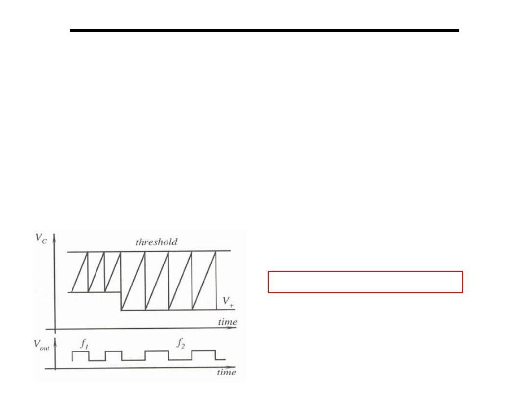
2.Voltage to Frequency Converter:
• When the threshold has been reached, an electronic switch
shorts the capacitor and discharges it.
• The switch then opens and allows the capacitor to recharge.
• The voltage on the capacitor is a triangular shape whose width
(i.e. the integration time) depends on the voltage at the
noninverting input.
• Since small changes in frequency can be easily detected, this is
a very sensitive method of digitization for small signal sensors.
HW: Find the conversation time
Analogue to Digital Converter
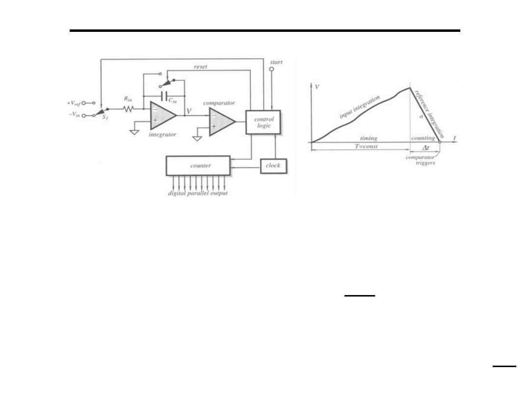
3.Dual Slop A to D Converter:
• The simpler (and slower) of the true A/D converters
• Based on the following principle: a capacitor is charged from the
voltage to be converted through a resistor, for a fixed,
predetermined time T. The capacitor reaches a voltage V
T
which
is:
• At time T, Vin is disconnected
• A negative reference voltage of known magnitude is connected
to the capacitor through the same resistor.
• This discharges the capacitor down to zero in a time
∆
T
V
T
= V
i n
T
R C
−
V
T
=
−
V
r e f
∆
T
R C

Analogue to Digital Converter
3.Dual Slop A to D Converter:
• Since these are equal in magnitude we have:
• In addition, a fixed frequency clock is turned on at the beginning
of the discharge cycle and off at the end of the discharge cycle.
Since
∆
T and T are known and the counter knows exactly how
many pulses have been counted, this count is the digital
representation of the input voltage
• The method is rather slow with approximately 1/2T conversions
per second.
• It is also limited in accuracy by the timing measurements,
accuracy of the analog devices and, of course, by noise.
• High frequency noise is reduced by the integration process and
low frequency noise is proportional to T (the smaller T the less
low frequency noise).
V
i n
T
R C
= V
r e f
∆
T
R C
→
V
i n
V
r e f
=
∆
T
T
Analogue to Digital Converter
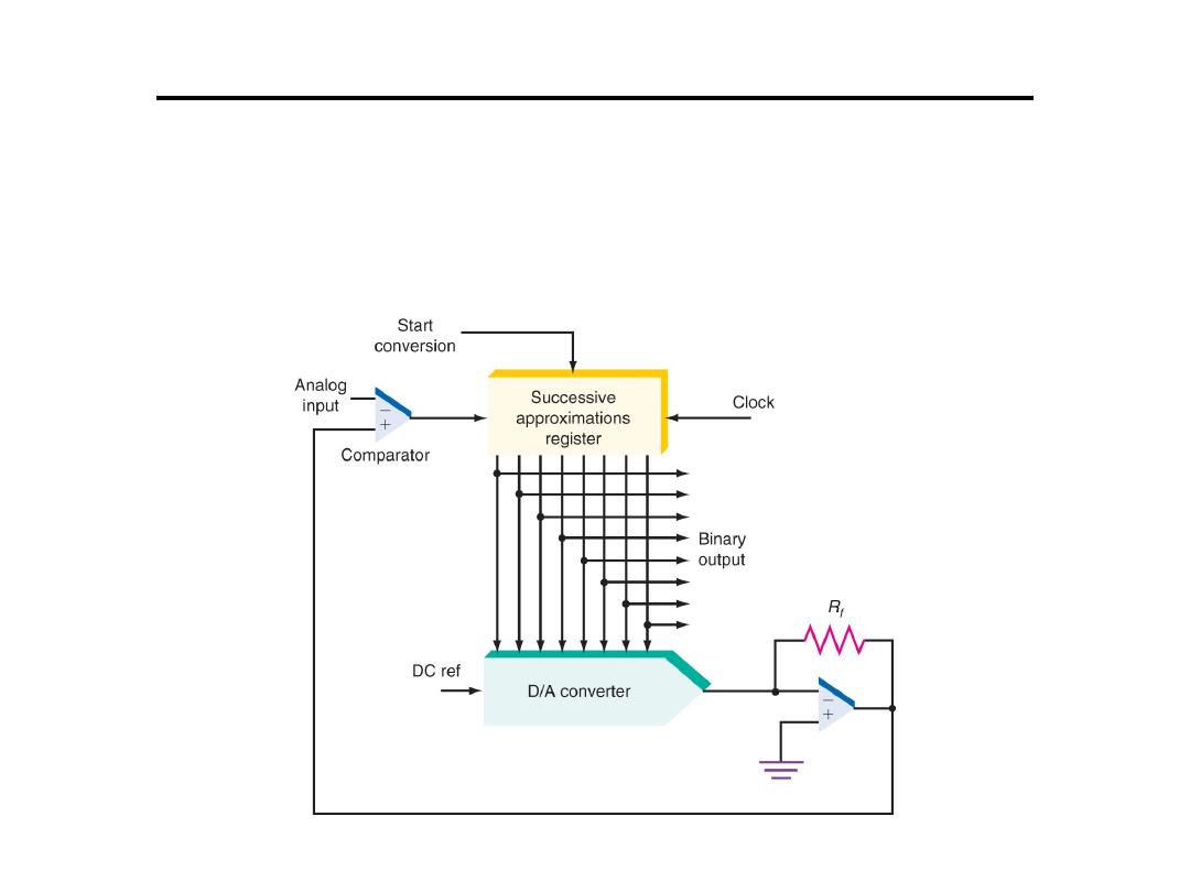
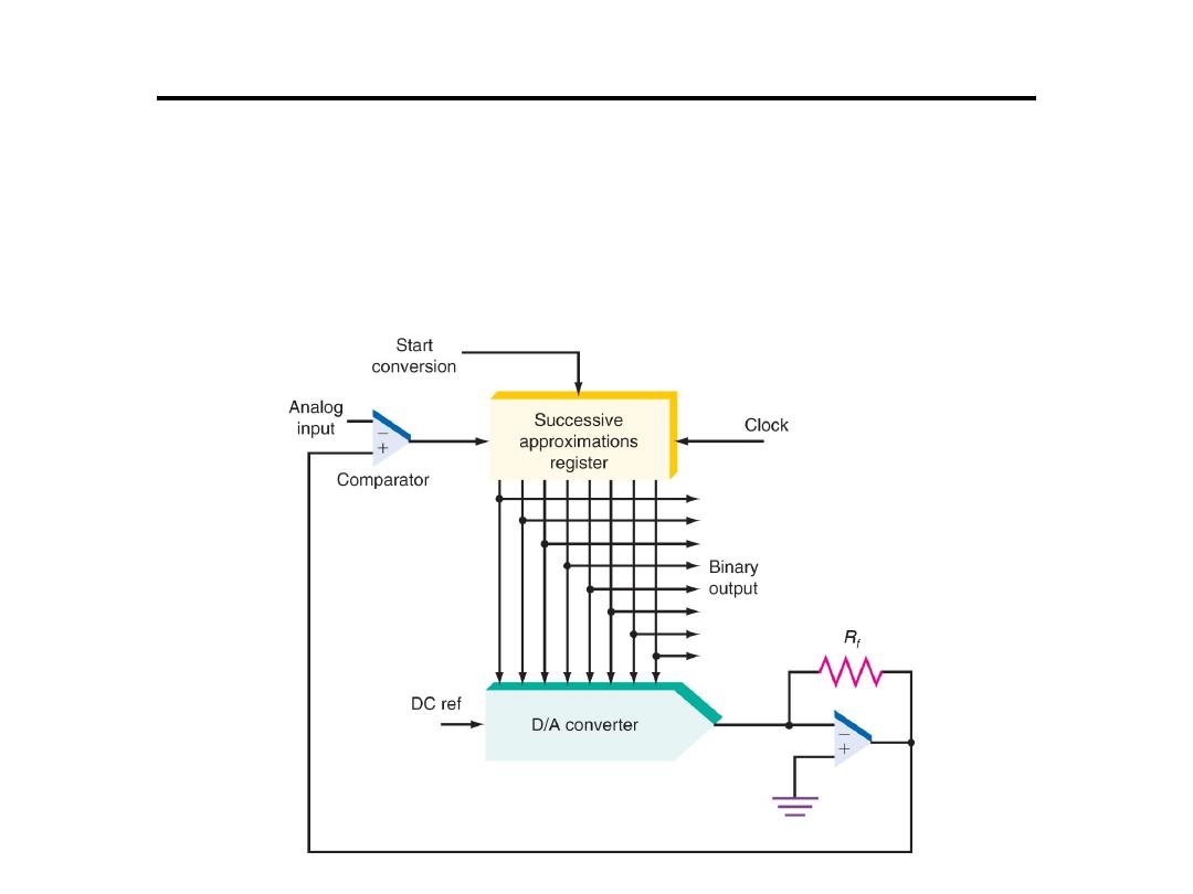
4. Successive-approximation converter:
This
converter contains an 8-bit successive-approximations
register (SAR).

Analogue to Digital Converter
4. Successive-approximation converter:
• Special logic in the register causes each bit to
be turned on one at a time from MSB to LSB
until the closest binary value is stored in the
register.
• At each clock cycle, a comparison is made.
– If the D/A output is greater than the analog input,
that bit is turned off (set to 0)
– If the D/A output is less than the analog input, that
bit is left on (set to 1).
• Process repeats until 8 bits are checked.
Analogue to Digital Converter
• If the clock frequency is 200-kHz, how long
does it take to complete the conversion for an
8-bit D/A converter?
Analogue to Digital Converter
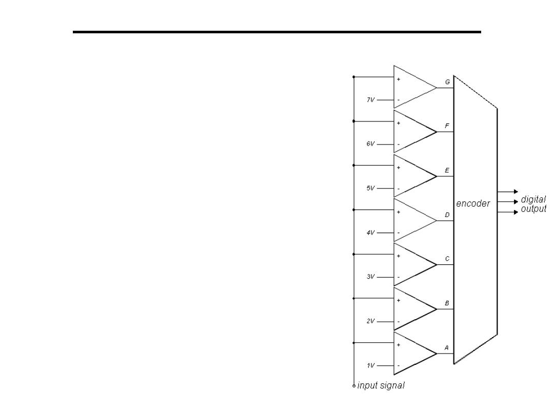
5. Flash A to D Converter:
•
Uses a reference and a comparator for
each of the discrete levels represented in
the digital output
•
Number of comparators =
number of quantization levels
•
Not practical for more than 10 bit
converters generally fast but expensive
Basics of Data Acquisition
•Full Scale Range (FSR):Full scale range refers to the largest
voltage range which can be input into the A/D converter
•Range: Range is an input span for an A/D and D/A system
Typical ranges are based on available sensors
–Unipolar (positive)
0 to 5 volts
0 to 10 volts
–Bipolar
-5 to 5 volts
-10 to 10 volts
+
10v
0v
+
10v
+
1.25v
-
10v
-
1.25v
FSR = 10v
FSR = 20v
FSR = 2.5v

Getting signals into the computer:
•Transducers convert physical variables into electrical outputs
•An input transducer (sensor) then supplies its output to signal
conditioning circuitry (on a Screw Terminal Panel)
•Signal conditioning circuitry prepares for interfacing with the PC
Amplification:
•The output of a sensor usually requires amplification
•Apply gain
Gain
•A scale (multiplying) factor which increases an input
signal to better utilize the range of the A/D converter
•Gain is the amplification applied to a signal to bring it to
the range of the A/D system
Basics of Data Acquisition
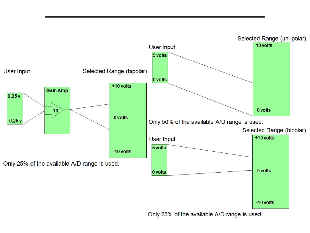
Selecting Gain and Range
Basics of Data Acquisition

Selecting the Best Gain & Range
•Analog input and output boards are generally designed to
interface to the majority of sensors that are available
•The ranges used on I/O boards may not always be appropriate
for every application
•Determine the maximum range that the input signal will use
•Determine if the signal is uni-polar (above zero) or bipolar
(above and below zero)
•Evaluate the available gain and range combinations to select the
most appropriate product
Basics of Data Acquisition

Resolution of the converter indicates the number of discrete values it can
produce.
Usually expressed in bits.
For example, an ADC that encodes an analog input to one of 256 discrete
values has a resolution of eight bits, since 2
8
= 256.
Resolution can also be defined electrically, and expressed in volts. The voltage
resolution of an ADC is equal to its overall voltage measurement range
divided by the number of discrete values. Some examples may help:
Example 1
•
measurement range = 0 to 10 volts
•
ADC resolution is 12 bits: 2
12
= 4095 quantization levels
•
ADC voltage resolution is: (10-0)/4095 = 0.00244 volts = 2.44 mV
Example 2
•
measurement range = -10 to +10 volts
•
ADC resolution is 14 bits: 2
14
= 16383 quantization levels
•
ADC voltage resolution is: (10-(-10))/16383 = 20/16383 = 0.00122 volts
= 1.22 mV
In practice, the resolution of the converter is limited by the
signal-to-noise ratio of the signal in question.
Basics of Data Acquisition

Accuracy depends on the error in the conversion.
Error has two components:
error
• non-
error (assuming the ADC is intended to be linear)
These errors are measured in a unit called the LSB, which is an abbreviation
In an eight-bit ADC, an error of one LSB is 1/256 of the full signal range, or
about 0.4%.
Quantization error is due to the finite resolution of the ADC, and is an
unavoidable imperfection in all types of ADC. The
of the
quantization error at the sampling instant is between zero and half of one
LSB.
All ADCs suffer from non-linearity errors caused by their physical
imperfections, causing their output to deviate from a linear function (or some
other function, in the case of a deliberately non-linear ADC) of their input.
Basics of Data Acquisition

Sampling: Analog signal is
in
and it is necessary to
convert this to a flow of digital values.
It is therefore required to define the rate at which new digital values are
sampled from the analog signal.
The rate of new values is called the sampling rate or
of
the converter.
A continuously varying bandlimited signal can be sampled and then the
original signal can be exactly reproduced from the discrete-time values by
However, this faithful reproduction is only possible if the sampling rate is
higher than twice the highest frequency of the signal. This is essentially
what is embodied in the
Shannon-Nyquist sampling theorem
Nyquist rate -- For lossless digitization, the sampling rate should be at
least twice the maximum frequency responses. Indeed many times more the
better.
Fs > 2.f
max
Since a practical ADC cannot make an instantaneous conversion, the input
value must necessarily be held constant during the time that the converter
performs a conversion.
An input circuit called a
performs this task—in most cases
by using a
to store the analogue voltage at the input, and using an
electronic switch or gate to disconnect the capacitor from the input.
Basics of Data Acquisition

EX: Design a conditioning circuit to connect a thermo couple of
output 2mV for 0
o
C and 20mV for 100
o
C to a (10V/8 bit) A to D
convertor . Find the error in the output of the A to D in
o
C.
Basics of Data Acquisition
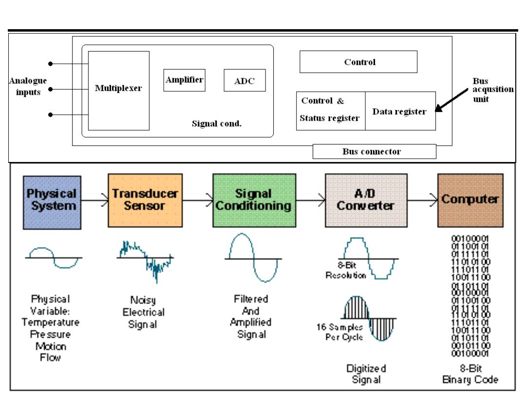
Data Acquisition System Block Diagram

Data Acquisition Board Specifications
1)Analogue Input:
1. Sampling rate: Determines how often conversions take place. Nyquist rate
2. Number of channels: Effective rate of each individual channel is inversely
proportional to the number of channels sampled.
EX: 100 KHz maximum,16
channels. 100 KHz/16 = 6.25 KHz per channel.
3. Resolution: smallest discernible change in the measured value.
4. Range: Minimum and maximum voltage levels that the A/D converter can
quantize.
5. Gain
2)Analogue Output:
1. Settling time: Time it takes to switch to a new channel, Each time a user
switches between channels, there is a delay, referred to as settling time
2. Slew rate: The Max. rate of change that the DAC can Produce on the o/p
signal.
3. Range: Minimum and maximum voltage levels that the D/A converter can
produce.
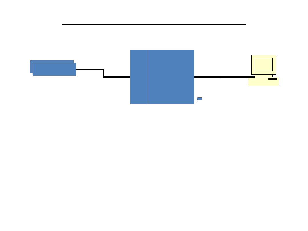
Data Acquisition System
• Data acquisitions system (DAQ) is an automated system to collect,
display and store data from detectors with the help of software.
• DAQ Hardware serves to convert analog signals from detectors to a
digital form and to perform initial processing. In our case comparators
convert analog pulses to digital logical signals which basically
indicate the presence of the input pulses, initial processing is finding
coincidences (i.e. occasions when some detectors are hit at the same
time).
• Other typical types conversions: TDC – Time to Digital Conversion
ADC – Amplitude to Digital Conversion. Other typical types of
processing: to find out whether a converted signal cross some
threshold value, to find how many detectors were hit, etc.
Detectors
Detectors
C
om
pa
ra
to
rs
Digital
Processor
(
FPGA
)
cables
cables
DAQ Hardware

Data Acquisition Software
• It can be the most critical factor in obtaining reliable, high
performance operation.
• Transforms the PC and DAQ hardware into a complete DAQ,
analysis, and display system.
• Different alternatives:
Programmable software:
Involves the use of a programming language,
such as:
– C++, Visual C++
– BASIC, Visual Basic + Add-on tools (such as VisuaLab with VTX)
• Advantage: flexibility
• Disadvantages: complexity and steep learning curve
– Data acquisition software packages.
• Does not require programming.
• Enables developers to design the custom instrument best suited to their
application.
• Examples: TestPoint, SnapMaster, LabView, DADISP, DASYLAB, etc.
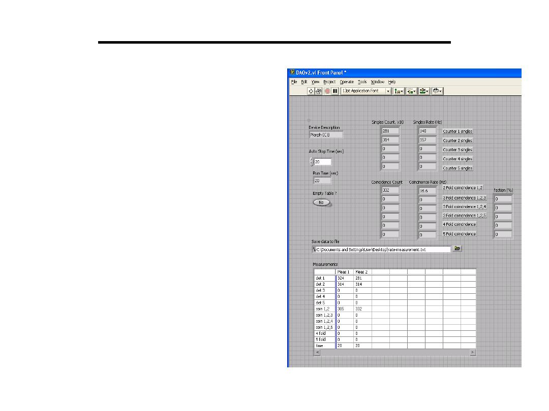
• The LabView program reads
out FPGA counters each
second and display count
changes from the moment
the program starts in the
screen
• The program can be run for
a predefined amount of time
(Auto Stop Time box)
• All the measurement are
summarized in the table in
the bottom. The content of
the table is also saved to an
ascii file and can be loaded
to MS Excel
Data Acquisition Software

Data Transmission in Digital Instruments
•A microcomputer-based data acquisition system is
interfaced to other devices.
•Data transmission and receiving are preferably done in
digital form since digital signals are less sensitive to
noise and interference than analog signals.
•Data are transmitted as either parallel (all bits are
transmitted simultaneously) or series (transmit 1 bit at
a time) Parallel data transmission is limited to certain
distance. Although there are techniques which permits
extending the range for parallel transmission, these are
complex and costly.
•Serial transmission is frequently used whenever data
are to be transmitted over a significant distance.
•Since serial data travel along one single path and are
transmitted 1 bit at a time, the cabling costs for long
distances are relatively low.

Data Transmission in Digital Instruments
Serial Data Transmission (STD): it has two modes:
• Simplex - transmission in one direction only, requires only one
transmitter and receiver
• Duplex - permits transmission in either direction, can occur in
two forms:
Half-duplex - transmission can be done on both direction but
cannot occur simultaneously.
Full-duplex – can transmit on both directions simultaneously
by means of four wires.
oThe data rate is measured in bits/sec (or baud abbreviated as 1
Bd), since the data are transmitted 1 bit at a time.
oTypical data rates are standardized; the most common rates (PC
modem connections) are 300, 600, 1200, and 2400 Bd.
oExamples of serial data transmission are: RS-232 Standard or
USB.

Data Transmission in Digital Instruments
Parallel Data Transmission (PDT): it has two modes:
• Synchronous – timing clock pulse is transmitted along with the
data. Transmission is very fast but requires a more complex system
• Asynchronous – does not take place at a fixed clock rate but
requires a handshake protocol between sending and receiving end.
Parallel data transmission occurs most frequently according to the
IEEE 488 Standard:
Bus permits connection of up to 15 instruments and data rates of up
to 1 Mbyte/sec.
Limitation– maximum total length of the bus cable is 20 m
The signals transmitted are TTL-compatible and employ negative
logic, where by a logic 0 corresponds to a TTL high state (>2V) and
a logic 1 to a TTL low state (<0.8V).
The 8-bit word transmitted over the IEEE 488 bus is coded in
ASCII format.

(SDT): Old Faithful: RS-232C
RS-232C is a serial communication interface standard
that has been in use, in one form or another, since the
1960s. RS-232C is used for interfacing serial devices
over cable lengths of up to 25 meters and at data rates of
up to 38.4 kbps. You can use it to connect to other
computers, modems, and even old terminals (useful
tools for monitoring status messages during debugging).
In days of old, printers, plotters, and a host of other
devices came with RS-232C interfaces. With the need to
transfer large amounts of data rapidly, RS-232C is being
supplanted as a connection standard by high-speed
networks, such as Ethernet. However, it can still be a
useful and (importantly) simple connection tool for your
embedded system.

(SDT): Old Faithful: RS-232C
RS-232C is unbalanced, meaning that the voltage level of a data
bit being transmitted is referenced to local ground. A logic high
for RS-232C is a signal voltage in the range of -5 to -15 V
(typically -12 V), and a logic low is between +5 and +15 V
(typically +12 V). So, just to make that clear, an RS-232C high is
a negative voltage, and a low is a positive voltage, unlike the rest
of your computer's logic.
It's also not unheard of to see RS-232C systems still using 7-bit
data frames (another leftover from the '60s), rather than the more
common 8-bit. In fact, this is one of the reasons why you'll still
see email being sent on the Internet limited to a 7-bit character
set, just in case the packets happen to be routed via a serial
connection that supports only 7-bit transmissions. It's nice how
pieces of history still linger around to haunt us! More commonly,
RS-232C data transmissions use 8-bit characters, and any serial
port you implement should do so, too.

(SDT): RS-422
Unlike RS-232C, which is referenced to local ground, RS-
422 uses the difference between two lines, known as a
twisted pair or a differential pair, to represent the logic
level. Thus, RS-422 is a balanced transmission, or, in other
words, it is not referenced to local ground. Any noise or
interference will affect both wires of the twisted pair, but
the difference between them will be less affected. This is
known as common-mode rejection. RS-422 can therefore
carry data over longer distances and at higher rates with
greater noise immunity than RS-232C. RS-422 can support
data transmission over cable lengths of up to 1,200 meters
(approximately 4,000 feet).
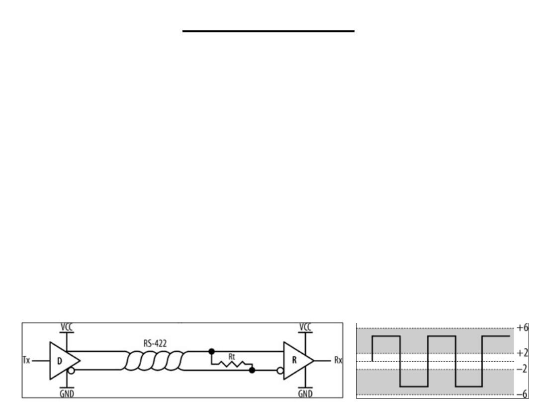
(SDT): RS-422
The figure shows a basic RS-422 link, where a driver (D) of one
embedded system is connected to a receiver (R) of another embedded
system via a twisted pair. The resistor, Rt, at receiving end of the
twisted pair is a termination resistor. It acts to remove signal
reflections that may occur during transmission over long distances,
and it is required. Rt is nominally 100-120 W.
The voltage difference between an RS-422 twisted pair is between ±4
V and ±12 V between the transmission lines. RS-422 is, to a degree,
compatible with RS-232C. By connecting the negative side of the
twisted pair to ground, RS-422 effectively becomes an unbalanced
transmission. It may then be mated with RS-232C. Since the voltage
levels of RS-422 fall within the acceptable ranges for RS-232C, the
two standards may be interconnected.

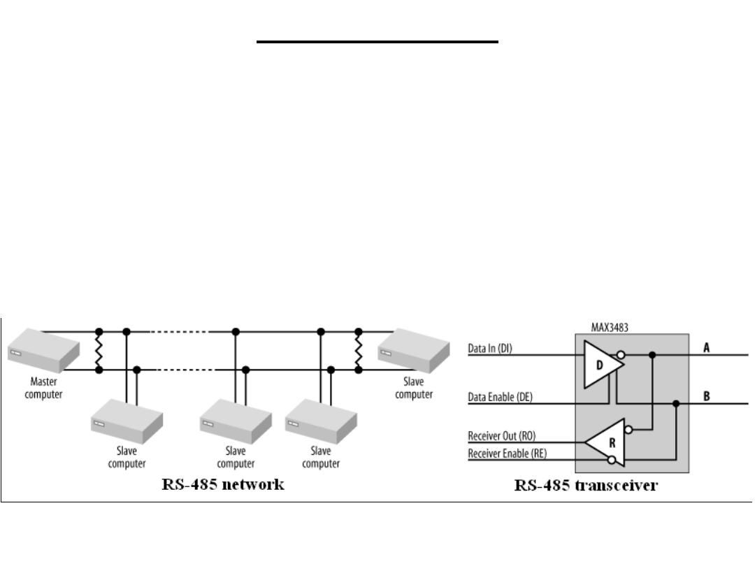
(SDT): RS-485
RS-485 is a variation on RS-422 that is commonly used for
low-cost networking and in many industrial applications. It
is one of the simplest and easiest networks to implement. It
allows multiple systems (nodes) to exchange data over a
single twisted pair.
RS-485 is based on a master-slave architecture. All
transactions are initiated by the master, and a slave will
transmit only when specifically instructed to do so. There
are many different protocols that run over RS-485, and often
people will do their own thing and create a protocol specific
to the application at hand. The interface to the RS-485
network is provided by a transceiver, such as a Maxim
MAX3483.
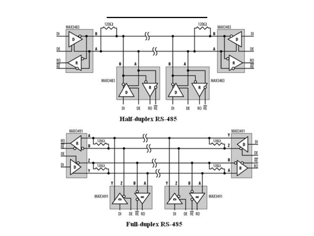
(SDT): RS-485
RS-485 may be implemented as half duplex, where a single
twisted pair is used for both transmission and reception, or
full duplex, where separate twisted pairs are used for each
direction. Full-duplex RS-485 is sometimes known as four-
wire mode. Note that for full-duplex operation, the
MAX3483s are replaced with MAX3491s that have dual
network interfaces.
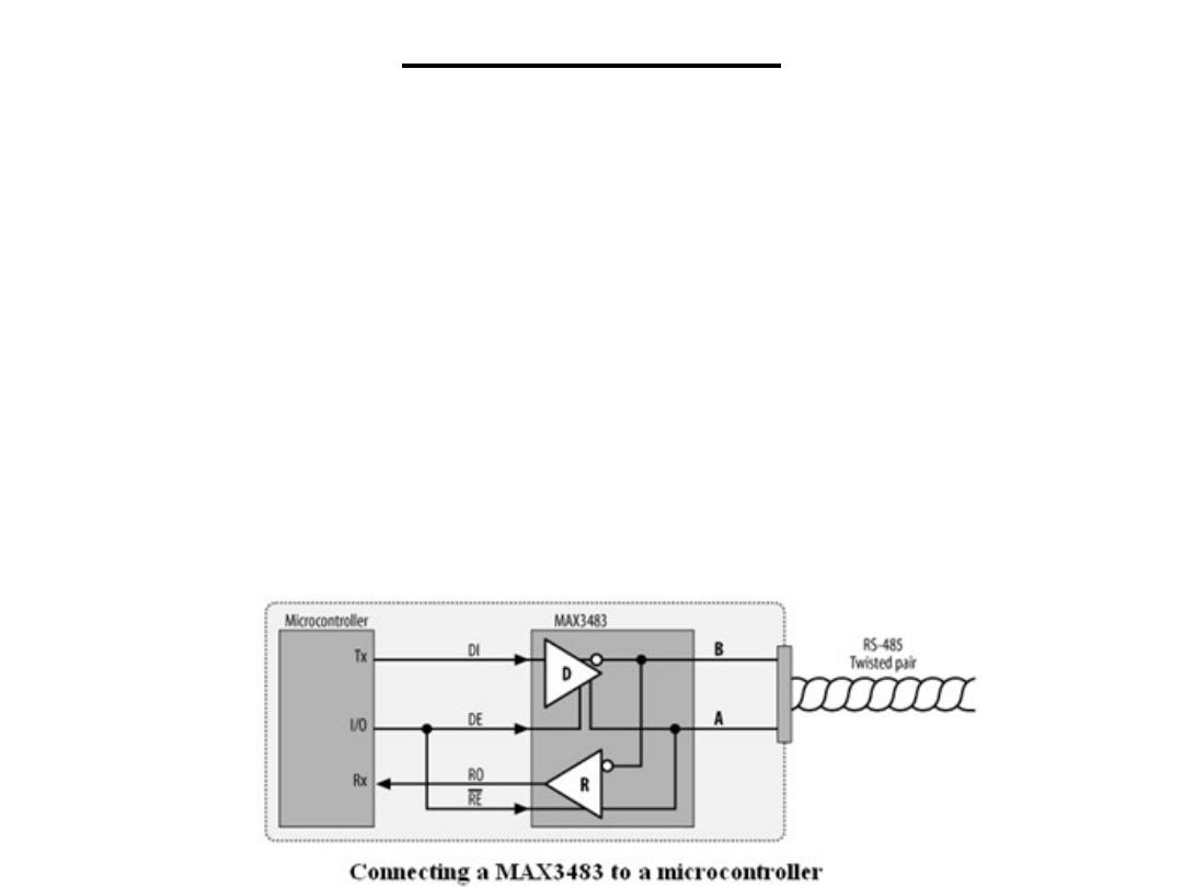
(SDT): RS-485
Normally, all systems connected to the RS-485 network have their receivers
enabled and listen to the traffic. Only when a system wishes to transmit does it
enable its driver. There are a number of formal protocols that use RS-485 as a
transmission medium, and twice as many homespun protocols as well. The
main problem you need to avoid is the possibility of two nodes of the network
transmitting at the same time. The simplest technique is to designate one node
as a master node and the others as slaves. Only the master may initiate a
transmission on the network, and a slave may only respond directly to the
master, once that master has finished.
The number of nodes possible on the network is limited by the driving
capability of the interface chips. Normally, this limit is 32 nodes per network,
but some chips can support up to 512 nodes.
(SDT): RS-485

(SDT): USB
Universal Serial Bus (USB) is the solution. It allows peripherals and computers
to interconnect in a standard way with a standard protocol and opens up the
possibility of "plug and play" for peripherals. USB is rapidly dominating the
desktop computer market, making RS-232C an endangered species. Therefore,
an understanding of USB (and how to build a USB port) is critical if you wish
to interface your embedded computer to the desktop machines of the near
future. USB supports the connection of printers, modems, mice, keyboards,
joysticks, scanners, cameras, and much more.
There are two specifications for USB: USB 1.1 and USB 2.0. USB 2.0 is fully
compatible with USB 1.1. USB supports data rates of 12 Mbps and 1.5 Mbps
(for slower peripherals) for USB 1.1, and data rates of 480 Mbps for USB 2.0.
Data transfers can be either isochronous(Occurring at equal intervals of time)
or asynchronous.
USB is a high-speed bus that allows up to 127 devices to be connected. No
longer is having only one or two ports on your computer a limitation. Further,
one standard for cables and connectors eliminates the confusion that existed
with RS-232C. Devices are able to self-identify to a host computer, and they
can be hot-swapped, meaning that the systems do not need to be powered
down before connection or disconnection.

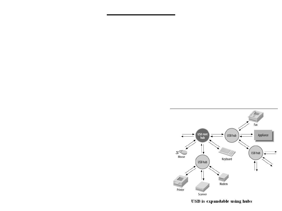
(SDT): USB
The basic structure of a USB network is a tiered star. A USB system
consists of one or more USB devices (peripherals), one or more hubs,
and a host (controlling computer). The host computer is sometimes
known as the host controller. Only one host may exist in a USB
network. The host controller incorporates a root hub, which provides
the initial attachment points to the host. The hubs form nodes to
which devices or other hubs connect, and they are (largely) invisible
to USB communication. In other words, traffic between a device and
a host is not affected by the presence of hubs.
Hubs are used to expand a USB network. For example, a given host
computer may have five USB ports. By connecting hubs, each with
additional ports, to the host, the physical connectivity of the system
is increased. Many USB devices, such as keyboards, incorporate
inbuilt hubs allowing them to provide additional expansion as well as
their primary function.
(SDT): USB
The host will regularly poll hubs for their status. When a new device is
plugged into a hub, the hub advises the host of its change in state. The
host issues a command to enable and reset that port. The device
attached to that port responds, and the host retrieves information about
the device. Based on that information, the host operating system
determines what software driver to use for that device. The device is
then assigned a unique address, and its internal configuration is
requested by the host. When a device is unplugged, the hub advises the
host of the change in state when polled,
and the host removes the device from its
list of available resources. The detection
and identification of USB devices by
a host is known as bus enumeration.

(SDT): USB
There are four types of transfers that can take place over USB:
Control transfer is used to configure the bus and devices on the bus, and to
return status information.
Bulk transfer moves data asynchronously over USB.
Isochronous transfer is used for moving time-critical data, such as audio
data destined for an output device. Unlike a bulk transfer, which can be
bidirectional, an isochronous transfer is uni-directional and does not include a
cyclic-redundancy-check.
Interrupt transfer is used to retrieve (get) data at regular intervals, ranging
from 1 to 255 milliseconds.
Data is transferred between USB devices using packets, and a transfer can
comprise one or more packets. A packet consists of a SYNC
(synchronization), a PID (Packet ID), content (data, address, etc.), and a
CRC.
The SYNC byte phase locks the receiver's clock. This is equivalent to the start
bit of an RS-232C frame. The PID indicates the function of the packet, such
as whether it is a data packet or a setup packet.
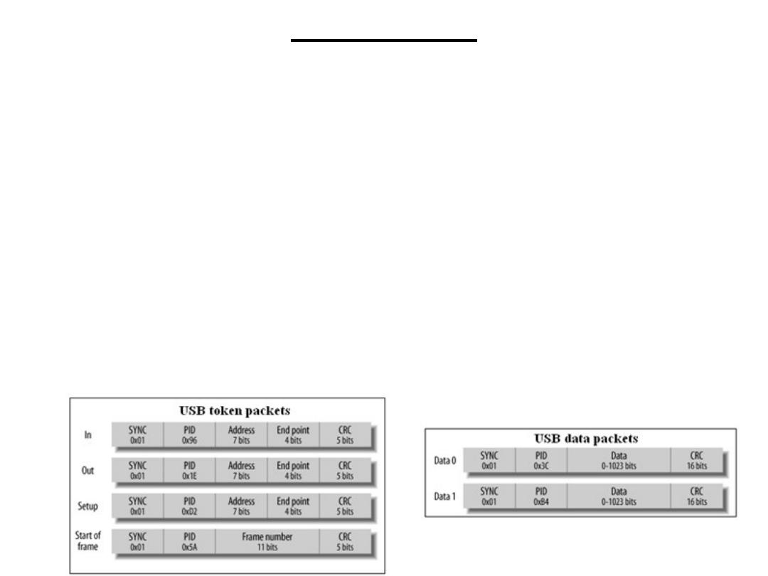
(SDT): USB
USB packets can be one of four types: token, data, handshaking, descriptor or
preamble:
Tokens are 24-bit packets that determine the type of transfer that is to take
place over the bus. There are four types of token packet. A token packet
consists of a SYNC byte, a packet ID (indicating packet type), the address of
the device being accessed by the host, the end-point address, and a 5-bit CRC
field. The end-point address is the internal destination of the data within the
device.
Data packet are of two types of, known as DATA0 and DATA1. The
transmission of data packets alternates between the two types. A single data
packet can transfer between 0 and 1,023 bytes, and the data packet's CRC is
16 bits due to the larger packet size.
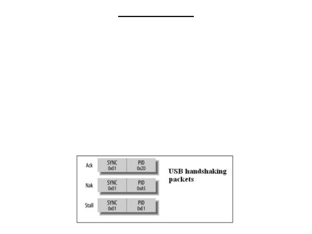
(SDT): USB
Handshaking packets are of three types. A successful data reception is
acknowledged with an Ack packet. The receiver notifies the host of a failed
transmission by sending a Nak (No Acknowledge) packet. A Stall is used to
pause a transfer.
A descriptor is a data packet used to inform the host of the capabilities of the
device. It contains an identifier for the device's manufacturer, a product
identifier, class type, and the device's internal configuration, such as its power
needs and end points. Each manufacturer has a unique ID, and each product in
turn will also have a unique ID. Software on the host computer uses
information obtained from a descriptor to determine what services a device
can perform and how the host can interact with that device.
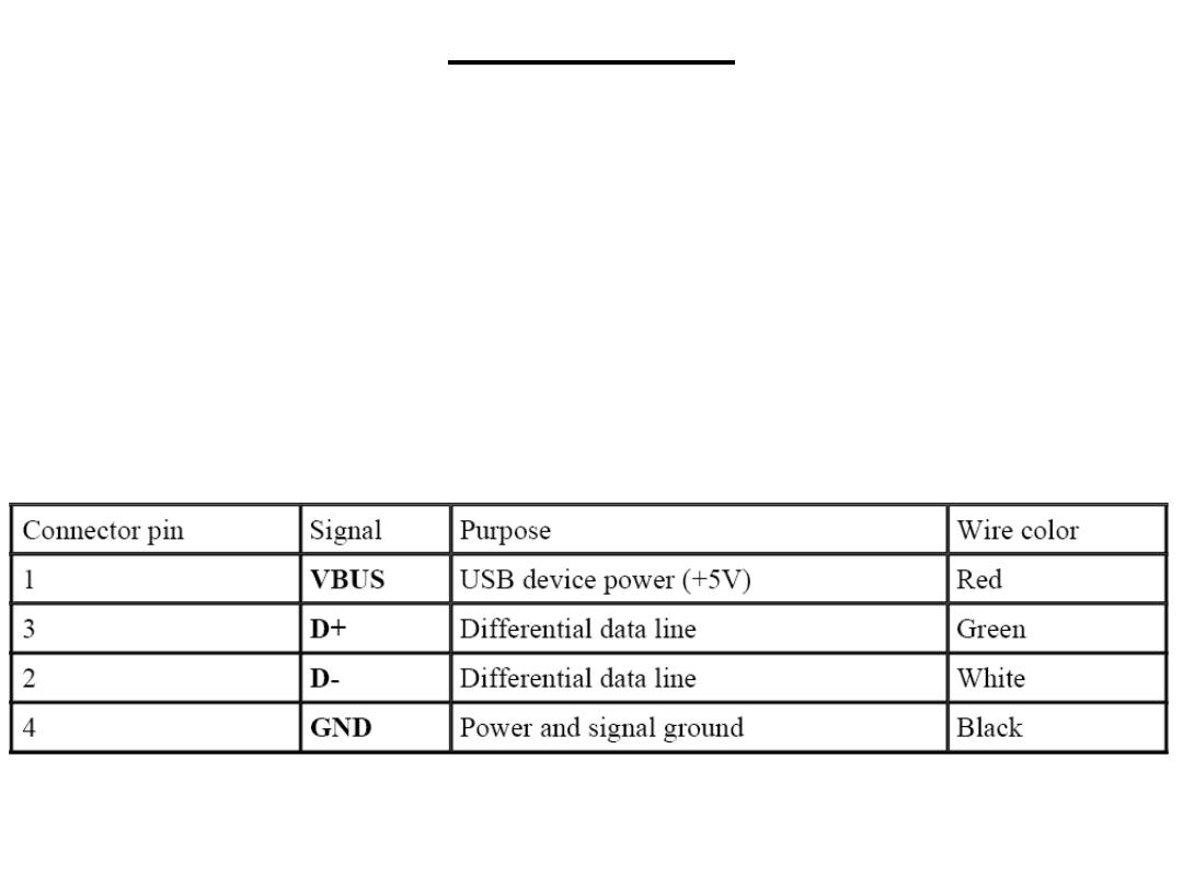
(SDT): USB
USB uses a shielded, four-wire cable to interconnect devices on the
network. Data transmission is accomplished over a differential twisted
pair (much like RS-422/485) labeled D+ and D-. The other two wires
are VBUS, which carries power to USB devices, and GND. Devices
that use USB power are known as bus-powered devices, while those
with their own external power supply are known as self-powered
devices. To avoid confusion, the wires within a USB cable are color-
coded.
(SDT): USB
The connection from a device back to a host is known as an upstream
connection. Similarly, connections from the host out to devices are
known as downstream connections. Different connectors are used for
upstream and downstream ports, with the specific intention of
preventing loopback. The only way to connect a USB network is a
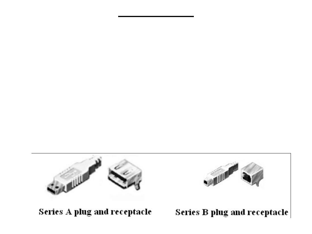
tiered star. USB uses two types of plugs (jacks) and two types of
receptacles (sockets) for cables and equipment. The first type is Series
A, shown in Figure, Series A connectors are for upstream connections.
In other words, a series A receptacle is found on a host or hub, and a
series A plug is at the end of the cable that attaches to the host or hub.

(SDT): IrDA
IrDA is the infrared transmission standard commonly used in
computers and peripherals (part of a device not connected to the main
device). IrDA, stands for "Infrared Data Association,“ used in
Hewlett-Packard calculators, known as HP-SIR (Hewlett-Packard
Serial Infra Red). The IrDA standard has expanded on HP-SIR
significantly and provides a range of protocols that application
software may use in communication.
The basic purpose of IrDA is to provide device-to-device
communication over short distances. Mobile devices, such as laptops,
present a problem when they must be connected to other machines or
networks. When the users are nontechnical types, this can be a real
problem. IrDA was developed as the solution to this problem. With
IrDA, no cables are required, and standard protocols ensure that
devices can exchange information seamlessly.
(SDT): IrDA
The expectation is that the IrDA user will be a mobile professional using a laptop
or PDA to communicate with other computers, PDAs, or peripherals nearby. This
concept has a number of important consequences. The devices communicating will
be physically close, so relatively low power transmissions are all that is required.
This is important because there are regulations guarding the maximum level of IR
radiation that can be emitted. Also, it is reasonable to assume that the two devices
that are to communicate will be physically pointed toward each other prior to use.
With all that in mind, IrDA is a point-to-point protocol that uses asynchronous
serial transmission over short distances. The initial IrDA specification (1.0)
supported data rates of between 2,400 bps and 115.2 kbps over distances of one
meter.
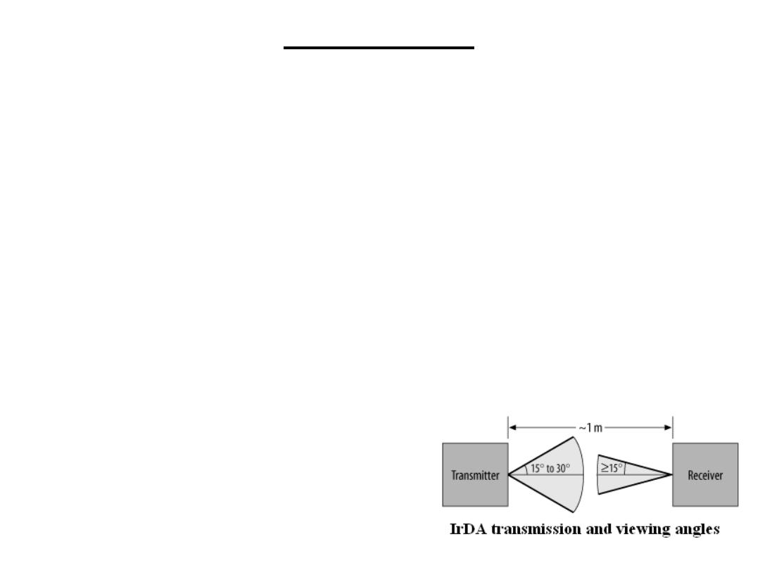
An IrDA transmitter will beam out its transmission at an angle of 15 degrees to 30
degrees on either side of the line of sight. The receiver has a "viewing angle“ of 15
degrees on either side
of its line of sight.
The standard data rates has been expanded
to support higher data rates of 1.152 Mbps
and 4 Mbps.

(SDT): IrDA
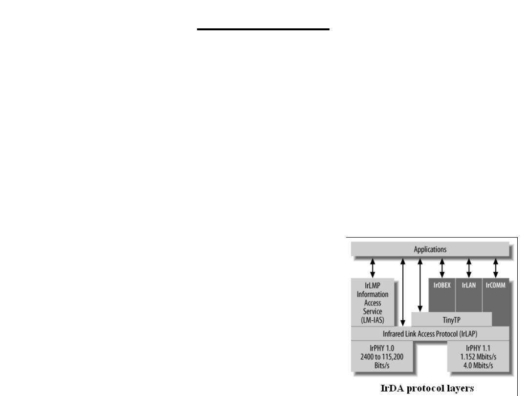
The IrDA standard specifies a number of protocol layers for
communication:
The IrPHY (IR Physical Layer) specification details the hardware layer,
including requirements for modulating the outputs of UARTs prior to
transmission.
The control protocol is known as High-level Data Link Control, or
HDLC. IrLAP (Infrared Link Access Protocol) uses a HDLC for
controlling access to the communication medium. One IrLAP exists per
device. An IrLAP connection is essentially a master-slave configuration, or,
as they are known in IrDA parlance, primary and secondary devices. The
primary device starts communication, sends commands, and handles data-
flow control (handshaking). It is rare for a primary device to be anything
other than a computer. Secondary devices (such as printers) simply respond
to requests from primaries. Two primary devices can communicate by one
primary assuming the role of a secondary device. Typically, the device that
initiates the transfer remains the primary, while the other device becomes a
secondary for the duration of the transaction.
(SDT): IrDA
IrLMP (Infrared Link Management Protocol) provides the device's software
with a means of sharing the single IrLAP between multiple tasks that wish to
communicate using IrDA. IrLMP also provides a query protocol by which one
device may interrogate another to determine what services are available on the
remote system. This query protocol is known as LM-IAS, or Link Management
Information Access Service. These are the basic IrDA protocols that all devices
must support.
IrCOMM provides emulation of standard serial-port and parallel-port devices.
IrLAN allows access to local area networks via the IR interface.
IrOBEX provides a mechanism for object exchange between devices, in
software that supports object-oriented programming.
Tiny TP is a lightweight protocol allowing
applications to perform flow-control
(handshaking) when transferring data
from one device to another.
(SDT): IrDA
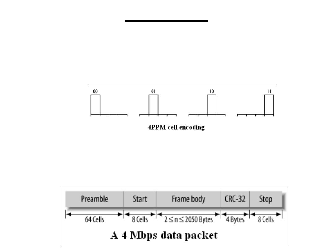
At data rates of 4 Mbps, PPM, or Pulse Position Modulation, is used to
distinguish different bits. With PPM, the position of the pulse is varied. Its
location within the subinterval determines the transmitted bit pattern. The
PPM used in IrDA is known as 4PPM and uses one of four positions to
provide the transmission of two data bits. In PPM terminology, these are
known as cells.
A sample data packet is shown below. It consists of a 64-cell (128-bit)
preamble packet, a start packet, the frame body containing the data to be
transmitted, a 32-bit Cyclic Redundancy Check (CRC) code, and a packet
stop marker. The data frame can be as little as 2 bytes or as large as 2050
bytes.
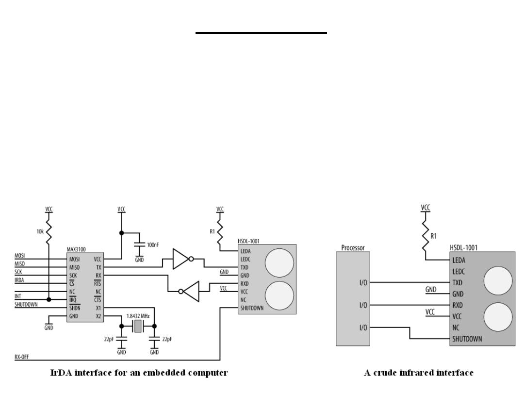
(SDT): IrDA
Your TV, VCR, DVD player, air conditioner, and a host of other
devices all have infrared ports for receiving commands from their
remote controls. The bad news is that none (or at least very few) are
IrDA-compliant. Appliance manufacturers tend to do their own thing,
and often at their own unusual baud rates too. So the circuit, to the left
below which is IrDA-compliant, may or may not work with a particular
application. However, something as simple as the circuit to the right
below may do the trick for you.

(SDT): Bluetooth
Bluetooth Basics: Bluetooth wireless technology is a short-range
communications technology intended to replace the cables
connecting portable and/or fixed devices while maintaining high
levels of security. The key features of Bluetooth technology are
robustness, low power, and low cost. The Bluetooth specification
defines a uniform structure for a wide range of devices to connect
and communicate with each other.
Bluetooth technology has achieved global acceptance such that any
Bluetooth enabled device, almost everywhere in the world, can
connect to other Bluetooth enabled devices in proximity. Bluetooth
enabled electronic devices connect and communicate wirelessly
through short-range, ad hoc networks known as piconets. Each
device can simultaneously communicate with up to seven other
devices within a single piconet. Each device can also belong to
several piconets simultaneously. Piconets are established
dynamically and automatically as Bluetooth enabled devices enter
and leave radio proximity.

(SDT): Bluetooth
Core Specification Versions: Version 2.0 + Enhanced
Data Rate (EDR), adopted November, 2004 Version 1.2,
adopted November, 2003
Specification Make-Up: Unlike many other wireless
standards, the Bluetooth wireless specification gives
product developers both link layer and application layer
definitions, which supports data and voice applications.
Spectrum: Bluetooth technology operates in the
unlicensed industrial, scientific and medical (ISM) band
at 2.4 to 2.485 GHz, using a spread spectrum, frequency
hopping, full-duplex signal at a nominal rate of 1600
hops/sec. The 2.4 GHz ISM band is available and
unlicensed in most countries

(SDT): Bluetooth
Interference: Bluetooth technology’s adaptive frequency
hopping (AFH) capability was designed to reduce
interference between wireless technologies sharing the
2.4 GHz spectrum. AFH works within the spectrum to
take advantage of the available frequency. This is done
by detecting other devices in the spectrum and avoiding
the frequencies they are using. This adaptive hopping
allows for more efficient transmission within the
spectrum, providing users with greater performance even
if using other technologies along with Bluetooth
technology. The signal hops among 79 frequencies at 1
MHz intervals to give a high degree of interference
immunity.

(SDT): Bluetooth
Range: The operating range depends on the device class:
• Class 3 radios – have a range of up to 1 meter or 3 feet
• Class 2 radios – most commonly found in mobile
devices – have a range of 10 meters or 30 feet
• Class 1 radios – used primarily in industrial use cases –
have a range of 100 meters or 300 feet
Power: The most commonly used radio is Class 2 and
uses 2.5 mW of power. Bluetooth technology is designed
to have very low power consumption. This is reinforced
in the specification by allowing radios to be powered
down when inactive.
Data Rate 1 Mbps for Version 1.2; Up to 3 Mbps
supported for Version 2.0 + EDR.

In the early 1970's, Hewlett-Packard came out with a standard bus
(HP-IB) to help support their own laboratory measurement
equipment product lines, which later was adopted by the IEEE in
1975. This is known as the IEEE Std.488-1975. The IEEE-488
Interface Bus (HP-IB) or general purpose interface bus (GP-IB) was
developed to provide a means for various instruments and devices to
communicate with each other under the direction of one or more
master controllers. The HP-IB was originally intended to support a
wide range of instruments and devices, from the very fast to the very
slow.
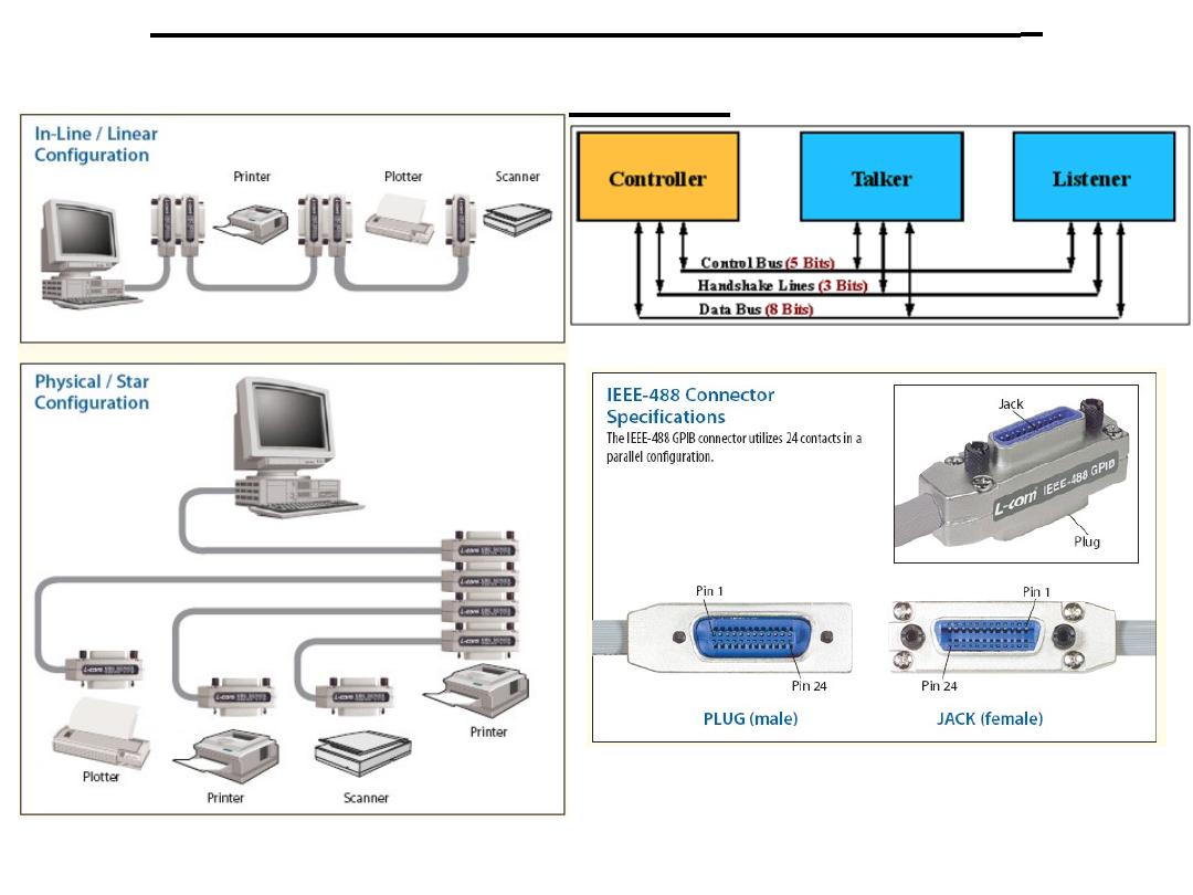
Description:
An 8-bit parallel asynchronous interface.
Very common in digital instrumentation application. Also known
as GPIB (general purpose instrument bus).
Consists of 16 bus lines where 8 are used to carry the data, 3 for
the handshaking protocol and the rest to control the data flow.
(PDT): General Purpose Interface
Bus(GPIB)
(PDT): General Purpose Interface
Bus(GPIB)
The HP-IB specification permits up to 15 devices to be
connected together in any given setup.
A device may be capable of any other three types of functions:
controller, listener, or talker.
A device on the bus may have only one of the three functions
active at a given time.
The maximum length of the bus network is limited to 20
meters total transmission path length.
(
PDT): General Purpose Interface
Bus(GPIB
)

(PDT): General Purpose Interface
Bus(GPIB)
Talkers, Listeners, and Controllers:
A GPIB device can be a Talker, Listener, and/or Controller:
•A Talker sends data to one or more Listeners
•A Listener accepts data from a Talker
•A Controller manages the flow of information over the bus.
EX:A GPIB Digital Voltmeter is acting as a Listener as its input
configurations and ranges are set, and then as a Talker when it actually
sends its readings to the computer.
The Controller is in charge of all communications over the bus. The
Controller’s job is to make sure only one device tries to talk at a time,
and make sure the correct Listeners are paying attention when the
Talker talks. Each GPIB system has a single system controller. The
system controller is ultimately in charge of the bus, and is in control as
the bus is powered up. There can be more than one Controller on the
bus and the System Controller can pass active control to another
controller capable device, though only one can be Controller In Charge
at a given time. The GPIB board is usually designated as the System
Controller.

(
PDT): General Purpose Interface
Bus(GPIB
)
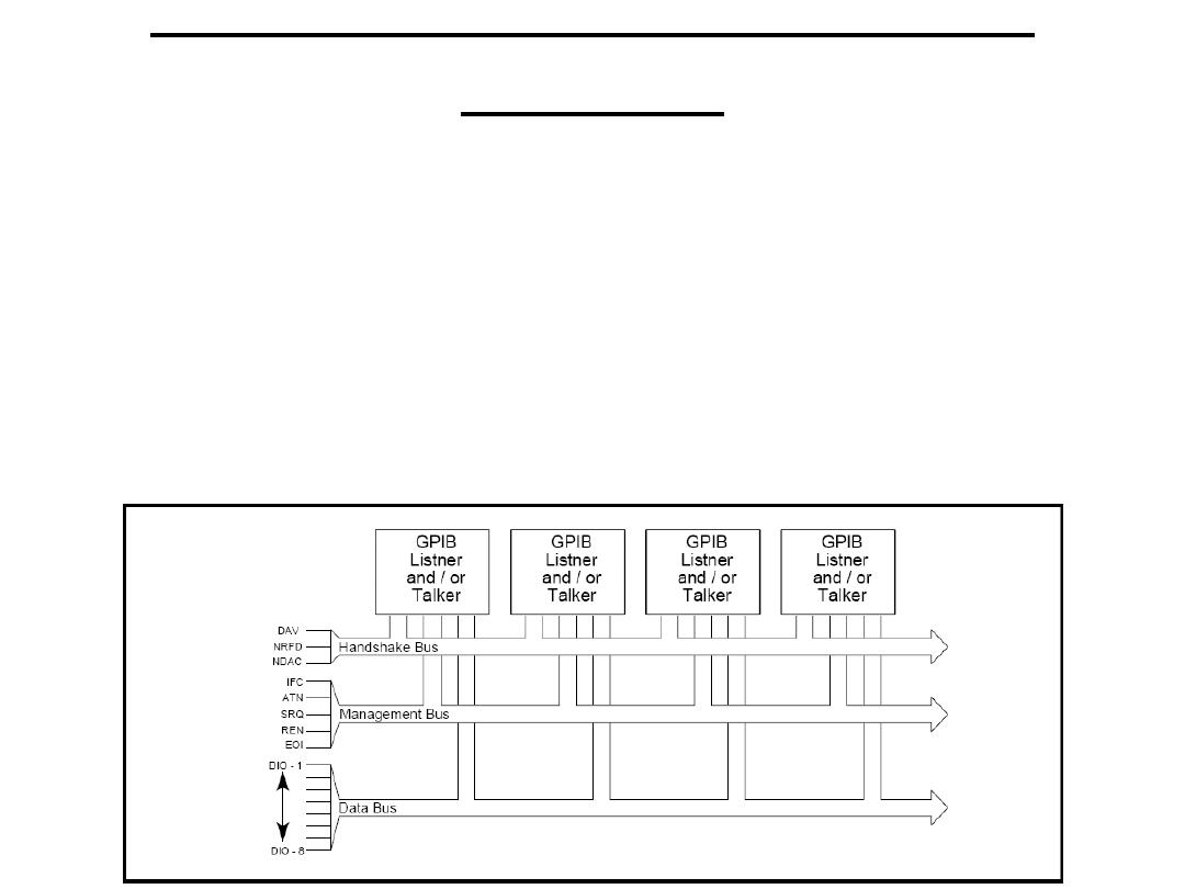
DATA LINES
DIO1 through DIO8 are the data transfer bits. Most
GPIB systems send 7-bit data
and use the eight bit as a parity or disregard it entirely
HANDSHAKING LINES
There are three handshaking lines that control the data
transfer between devices.
NRFD (Not Ready For Data): this bit is used to indicate
the readiness (or lack thereof) of a device to accept data
DAV (Data Valid): this bit is used to indicate to receiving
devices that data has been placed on the bus and is available
to read.
NDAC (Not Data Accepted): is asserted by the receiving
device to indicate that data has been read and may now be
removed from the bus.

(
PDT): General Purpose Interface
Bus(GPIB
)
SYSTEM MANAGEMENT LINES
ATN (Attention): is used by the controller to specify how data on the DIO
lines is interpreted and which devices must respond to the data
IFC (Interface Clear): is used by the system controller to place the entire
system in a known quiescent (Cleared) state and to assert itself as Controller
In Charge (CIC).
SRQ (Service Request): is used by a device on the bus to indicate the need
for attention and requests an interrupt of the current event sequence.
REN (Remote Enable): is used by the controller in conjunction with other
messages to place a device on the bus into either remote or local mode.
EOI (End or Identify): Is used by Talkers to indicate the end of a message
string, or is used by the Controller to command a polling sequence.
Polling, or polled operation, in computer science, refers to actively sampling the status of an external
device by a client program as a synchronous activity. Polling is most often used in terms of I/O, and is also
referred to as polled I/O.
Polled I/O is a system by which an operating system (OS) waits and monitors a device until the device is
ready to read. In early computer systems, when a program would want to read a key from the keyboard, it
would constantly poll the keyboard status port until a key was available; due to lack of multiple processes
such computers could not do other operations while waiting for the keyboard. The solution and alternative
to this approach is for the device controller to generate an interrupt when the device was ready to transfer
data. The CPU handles this interrupt and the OS knows to fetch the data from the relevant device registers.
This solution is called interrupt driven I/O.
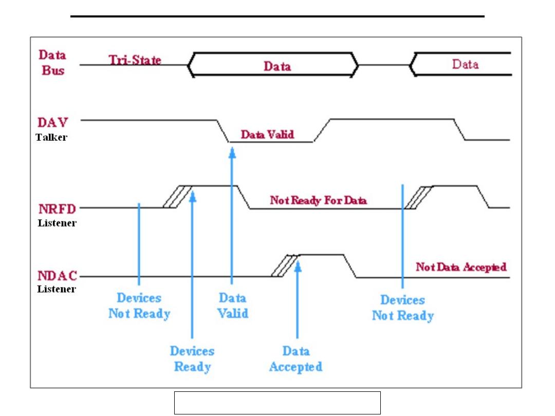
(PDT): General Purpose Interface
Bus(GPIB)
GPIB Bus Handshake Timing

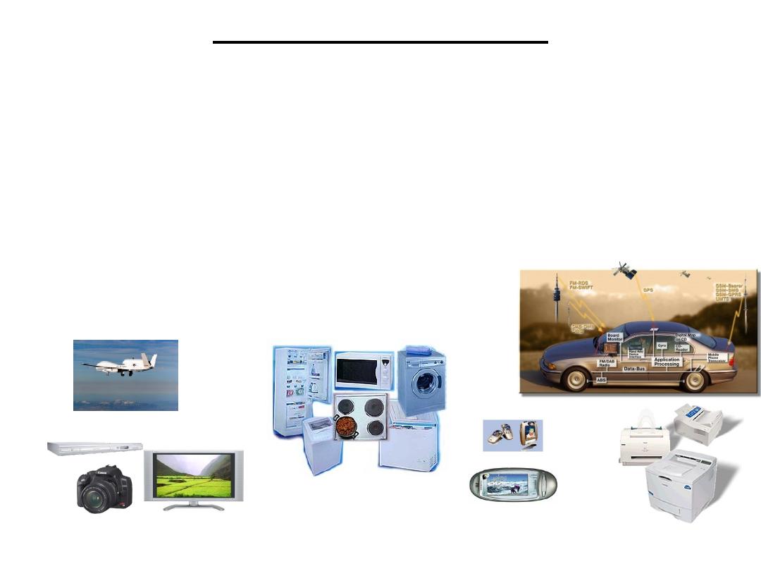
Embedded Systems
Definition 1) Any device that includes a programmable
computer but is not itself a general-purpose computer.
or 2) Embedded systems are computing systems with tightly
coupled hardware and software integration, that are designed
to perform a dedicated function.
Take advantage of application characteristics to optimize the
design:
• Don’t need all the general-purpose elements.
• But need to understand the application.
Household
Appliances
Automobile
Communication
Avionics
Consumer
Electronics
Office Equipments
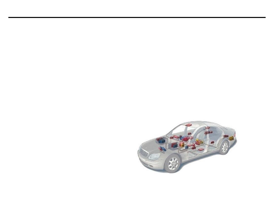
Example: Automotive Embedded Systems
• Today’s high-end automobile have > 80
microprocessors:
• 4-bit microcontroller checks seat belt;
• microcontrollers run dashboard devices;
• 16/32-bit microprocessor controls engine.
• Millions lines of code
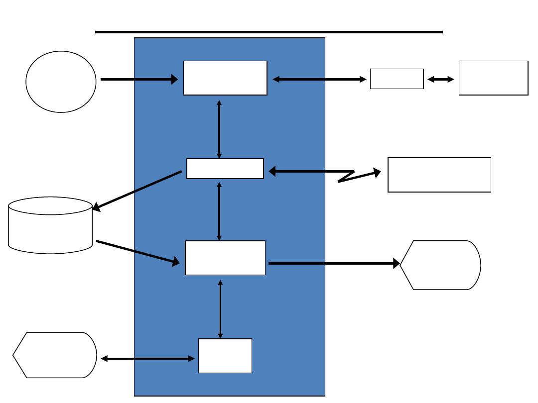
A Typical Embedded System
Algorithms for
Digital Control
Data Logging
Data Retrieval
and Display
Operator
Interface
Interface
Engineering
System
Remote
Monitoring System
Real-Time
Clock
Database
Operator’s
Console
Display
Devices
Real-Time Computer

Embedded Systems
Characteristics of Embedded Systems:
• Sophisticated functionality.
• Real-time operation.
• Low manufacturing cost.
• Low power.
• Short time-to-market and small teams.
Functional complexity:
• Often have to run sophisticated algorithms or multiple algorithms
.
– Example: A DVD player: DVD, video CD, audio CD, JPEG image CD, MP3 CD….
– Requiring domain-specific knowledge.
• Often provide sophisticated user interfaces.
– Multiple levels of user menus
– Support for multiple languages
– Graphics
– Speech, handwriting

Embedded Systems
Real-time operation:
• Must finish operations by deadlines.
– Hard real time: missing deadline causes failure.
– Soft real time: missing deadline results in degraded performance.
• Many systems are multi-rate: must handle operations at widely
varying rates.
– Example: Audio, Video
Cost and Power Consumption:
• Many embedded systems are mass-market items that must
have low manufacturing costs.
– Limited memory, microprocessor power, etc.
• Power consumption is critical in battery-powered devices.
– Excessive power consumption increases system cost even in wall-powered
devices.
Embedded Systems
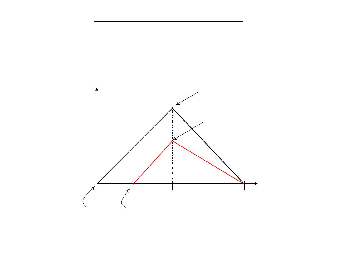
Time-to-market:
• Often must meet tight deadlines.
– 6 month market window is common.
On-time Delayed
entry entry
Peak revenue
Peak revenue from delayed
entry
Market rise
Market fall
W
2W
Time
D
On-time
Delayed
R
ev
en
ue
s
(
$
)
Challenges in Embedded System Design
• How much hardware do we need?
– How many processors? How big are they? How much memory?
• How do we meet performance requirements?
– What’s in hardware? What’s in software?
– Faster hardware or cleverer software?
• How do we minimize power?
– Turn off unnecessary logic?
– Reduce memory accesses?
• How do we ship in time?
– Off-the-shelf chips? IP-reuse?
• Does it really work?
– Is the specification correct?
– Does the implementation meet the specifications?
– How do we test for real-time characteristics?
– How do we test on real data?
• How do we reduce size/weight?

Challenges in Embedded System Design
Required Designers:
• Expertise with both
software
and
hardware
is needed to
optimize design metrics.
– Not just a hardware or software expert
– A designer must be comfortable with various technologies in order to
choose the best for a given application and constraints
– A designer must be able to communicate with teammates of various
background
Design methodologies:
• A procedure for designing a system.
• Understanding your methodology helps you ensure you didn’t
skip anything.
• Compilers, software engineering tools, computer-aided design
(CAD) tools, etc., can be used to:
– help automate methodology steps;
– keep track of the methodology itself.
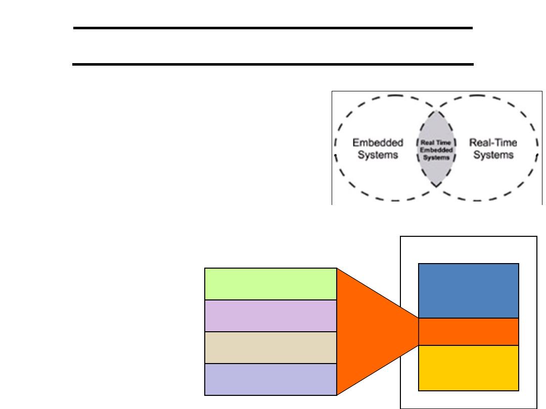
Relationship Between Real-Time
Systems and Embedded Systems
• Real-time embedded systems are those embedded system with real-
time behaviors.
• Legacy Software:
– Software is the most complex part of today's
safety critical embedded systems
– Most embedded systems are legacy designs
– Written in a low level language such as assembly language
– Existing tools do not address the verification problem
– Goal: Verify legacy code
with respect to
• a formal specification
• A high level design
• Safety properties
Embedded System
Real-Time OS
Application
Software
Hardware
Scheduler
Memory
Management
Inter-Process
Communication
Interface to
the hardware

Embedded System Processors & Memory
1)Processors: The processors found in common personal computers (PC) are
general-purpose or universal processors. They are complex in design
because these processors provide a full scale of features and a wide spectrum
of functionalities.
One class of embedded processors focuses on size, power consumption, and
price. Therefore, some embedded processors are limited in functionality, i.e.,
a processor is good enough for the class of applications for which it was
designed but is likely inadequate for other classes of applications.
2)Memories:
A.Read Only Memory (ROM):With non-volatile content and without the
need for an external power source.
• Mask Programmed ROM—the memory content is programmed during the
manufacturing process. Once programmed, the content cannot be changed. It
cannot be reprogrammed.
• Field Programmable ROM (PROM)—the memory content can be
custom-programmed one time. The memory content cannot change
once programmed.

Embedded System Processors & Memory
• Erasable Programmable ROM (EPROM)—an EPROM device can be
custom-programmed, erased, and reprogrammed as often as required within
its lifetime (hundreds or even thousands of times). The memory content is
non-volatile once programmed. Traditional EPROM devices are erased by
exposure to ultraviolet (UV) light. An EPROM device must be removed
from its housing unit first. It is then reprogrammed using a special hardware
device called an EPROM programmer.
• Electrically Erasable Programmable ROM (EEPROM or E2PROM)—
modern EPROM devices are erased electrically and are thus called
EEPROM. One important difference between an EPROM and an EEPROM
device is that with the EEPROM device, memory content of a single byte
can be selectively erased and reprogrammed. Therefore, with an EEPROM
device, incremental changes can be made. Another difference is the
EEPROM can be reprogrammed without a special programmer and can stay
in the device while being reprogrammed.
• Flash Memory—the flash memory is a variation of EEPROM, which allows
for block-level (e.g., 512-byte) programmability that is much faster than
EEPROM.

Embedded System Processors & Memory
B.Random Access Memory (RAM):Also called Read/Write Memory,
requires external power to maintain memory content. The term random
access refers to the ability to access any memory cell directly. RAM is
much faster than ROM. Two types of RAM that are of interest:
• Dynamic RAM (DRAM)—DRAM is a RAM device that requires periodic
refreshing to retain its content.
• Static RAM (SRAM)—SRAM is a RAM device that retains its content as
long as power is supplied by an external power source. SRAM does not
require periodic refreshing and it is faster than DRAM.
• Non-Volatile RAM (NVRAM)—NVRAM is a special type of SRAM that
has backup battery power so it can retain its content after the main system
power is shut off. Another variation of NVARM combines SRAM and
EEPROM so that its content is written into the EEPROM when power is
shut off and is read back from the EEPROM when power is restored.

Operating System
• An OS is a system program that provides an interface
between application programs and the computer
system (hardware)
– Primary Functions
• Provide a system that is convenient to use.
• Organize efficient and correct use of system resources.
– Four main tasks of OS:
1)Process Management
• Process creation
• Process loading
• Process execution control
• Interaction of the process with signal events
• Process monitoring
• CPU allocation
• Process termination

Operating System
2)Inter-process Communication
• Synchronization and coordination
• Deadlock detection
• Process Protection
• Data Exchange Mechanisms
3)Memory Management
• Services for file creation, deletion, reposition and protection
4)Input / Output Management
• Handles requests and release subroutines for a variety of
peripherals and read, write and reposition programs.
–Operating system components:
• Real-time clock: Provides information for process scheduling.
• Interrupt handler: Manages aperiodic requests for service.
• Scheduler: Chooses the next process to be run.
• Resource manager: Allocates memory and processor resources.
• Dispatcher: Starts process execution.

Operating System & Real Time
Some core functional similarities between a typical RTOS and
GPOS include:
•Some level of multitasking,
•Software and hardware resource management,
•The condition of underlying OS services to applications.
•Abstracting the hardware from the software application.
On the other hand, some key functional differences that set
RTOS apart from GPOS include:
•Better reliability in embedded application contexts,
•The ability to scale up or down to meet application needs,
•Faster performance.
•Reduced memory requirements.
•Scheduling policies tailored for real-time embedded systems.
•Support for diskless embedded systems by allowing executables to boot and
run from ROM or RAM.
•Better portability to different hardware platforms.

Real-time operating systems
• Real-time operating systems are specialised operating systems
which manage the processes in the RTS.
• Responsible for process management and resource (processor
and memory) allocation.
• May be based on a standard kernel which is used unchanged or
modified for a particular application.
• Do not normally include facilities such as file management.
• A real-time operating system (RTOS) is a program that
schedules execution in a timely manner, manages system
resources, and provides a consistent foundation for developing
application code. Application code designed on an RTOS can
be quite diverse, ranging from a simple application for a
digital stopwatch to a much more complex application for
aircraft navigation. Good RTOSes, therefore, are scalable in
order to meet different sets of requirements for different
applications.
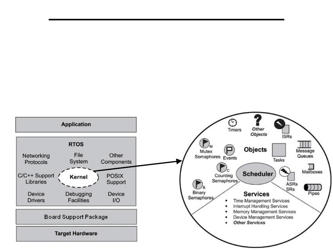
Real-time operating systems
• For example, in some applications, an RTOS comprises only a kernel,
which is the core supervisory software that provides minimal logic,
scheduling, and resource-management algorithms. Every RTOS has a
kernel. On the other hand, an RTOS can be a combination of various
modules, including the kernel, a file system, networking protocol
stacks, and other components required for a particular application, as
illustrated at a high level in figure.

Real-time operating systems
• Kernel (supervisor program):
– Manages the operating system
– Memory resident
– Loads set of programs that lies between applications software and the
hardware
– Fundamental software that controls non-resident portions of the OS as
needed
– Booting – Loads the kernel into memory
• Resources: A resource is (usually) hardware that needs to be accessed.
Typical Resources : 1)File system. (Data stored on disk) 2) Terminal I/O 3)
Main memory. 4) Sensors and actuators. 5) Network services (To connect to
other computers). 6) Threads. 7) CPU time.
• Task: A task, also called a thread, is a simple program that thinks it has the
CPU all to itself. The design process for a real-time application involves
splitting the work to be done into tasks which are responsible for a portion
of the problem. Each task is assigned a priority, its own set of CPU registers,
and its own stack area.
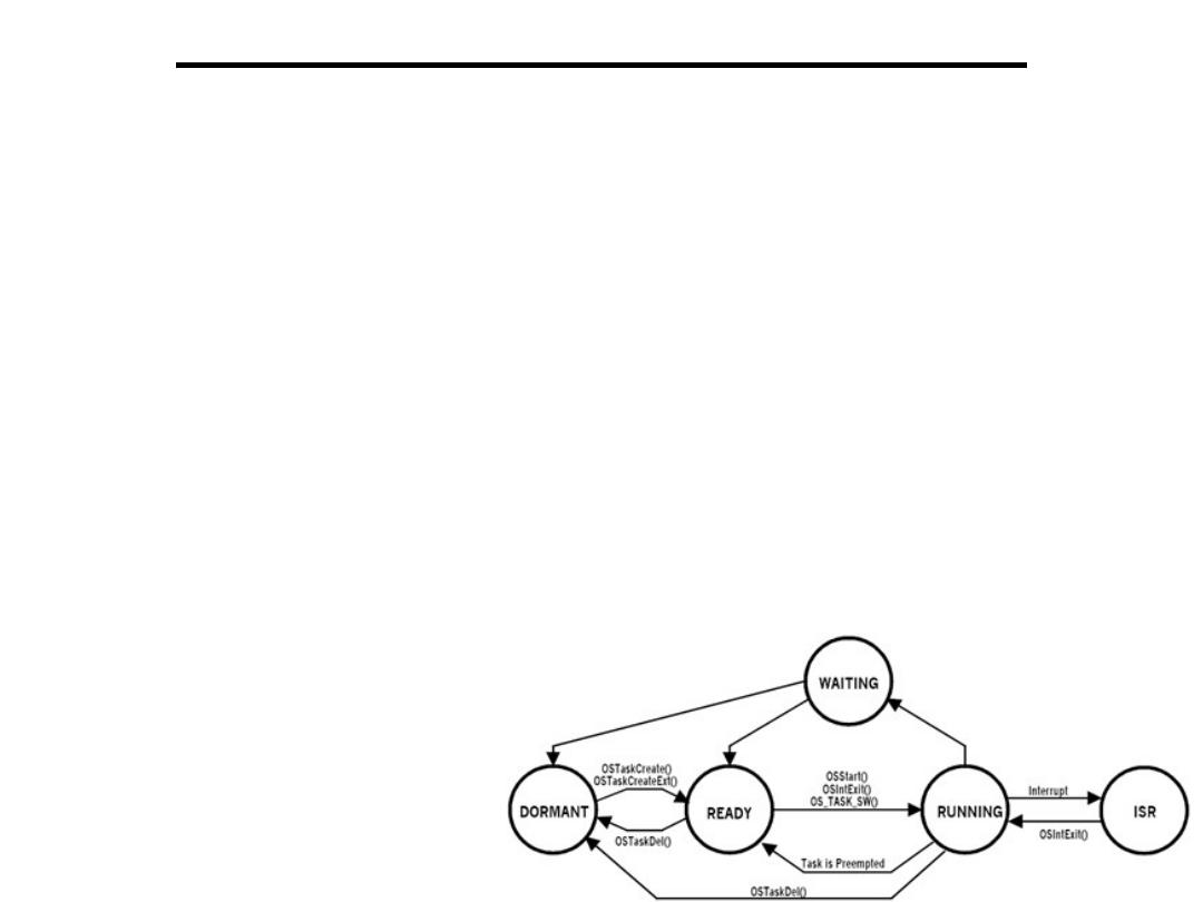
Real-time operating systems
•Each task typically is an infinite loop that can be in any one of five states:
DORMANT, READY, RUNNING, WAITING FOR AN EVENT, or
INTERRUPTED.
–The DORMANT state corresponds to a task which resides in memory but has
not been made available to the multitasking kernel.
–A task is READY when it can execute but its priority is less than the currently
running task.
–A task is RUNNING when it has control of the CPU.
–A task is WAITING FOR AN EVENT when it requires the occurrence of an
event (waiting for an I/O operation to complete, a shared resource to be
available, a timing pulse to occur, time to expire etc.).
–A task is INTERRUPTED when an interrupt has occurred and the CPU is in
the process of servicing the interrupt.
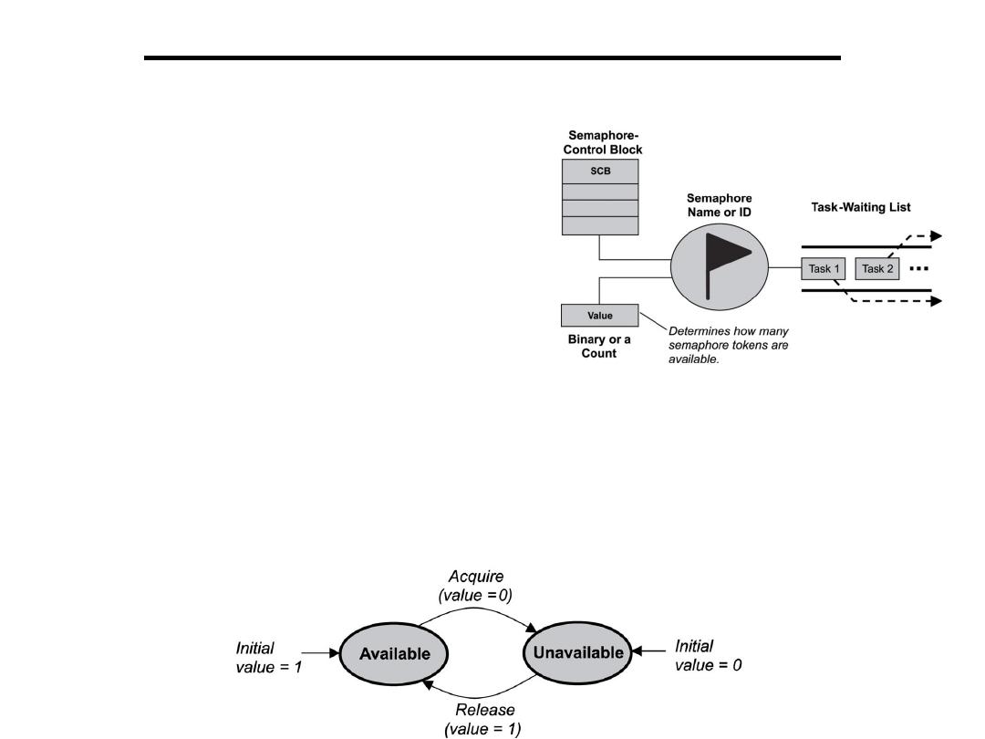
Real-time operating systems
• Semaphores: A semaphore (sometimes called a semaphore token) is a kernel
object that one or more threads of execution can acquire or release for the purposes
of synchronization or mutual exclusion.
• When a semaphore is first created, the kernel
assigns to it 1)an associated semaphore control
block (SCB) 2) a unique ID 3) a value (binary
or a count) 4) and a task-waiting list.
• Types of semaphores:
1)Binary Semaphores: A binary semaphore can have a value of either 0 or 1. When
a
binary semaphore’s value is 0, the semaphore is considered unavailable (or empty);
when the value is 1, the binary semaphore is considered available (or full ).
Binary semaphores are treated as global resources, which means they are shared
among all tasks that need them. Making the semaphore a global resource allows any
task to release it, even if the task did not initially acquire it.
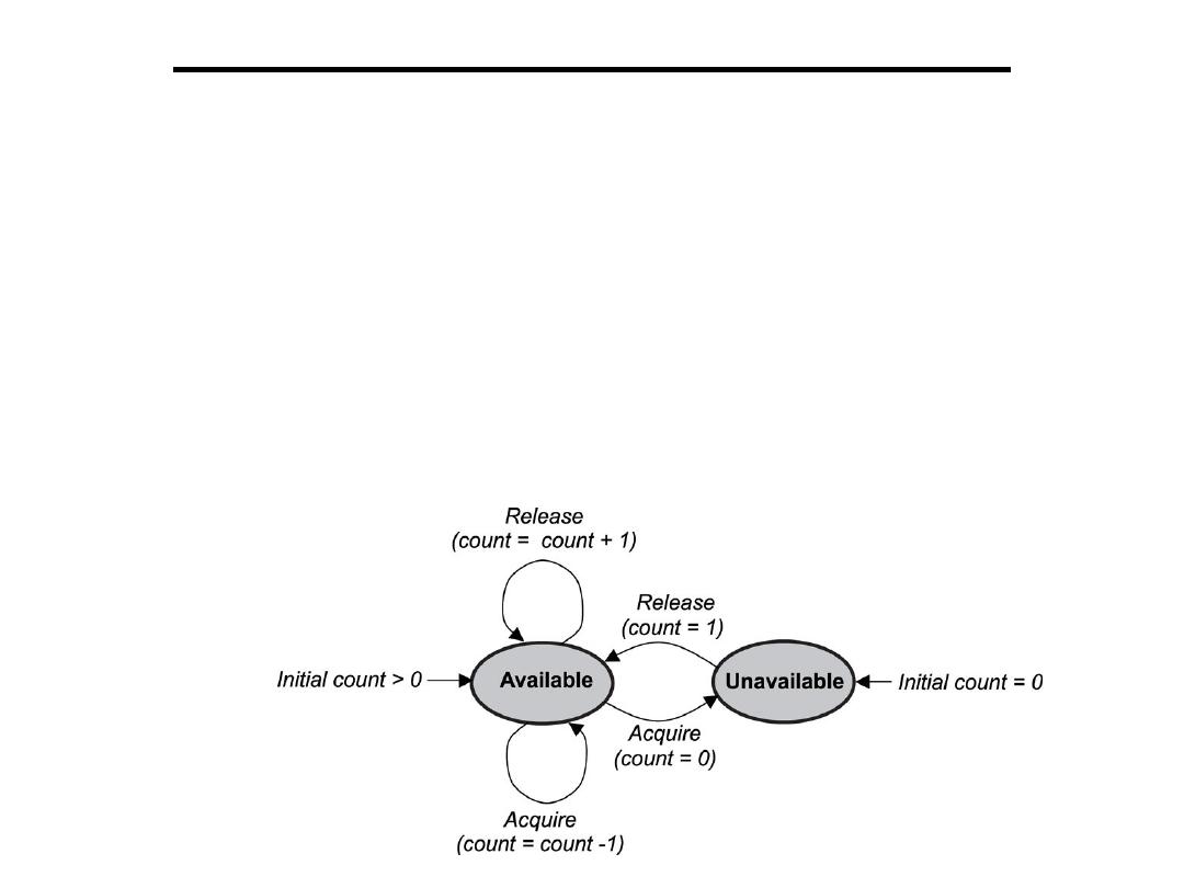
Real-time operating systems
2)Counting Semaphores: A counting semaphore uses a count to allow it to be
acquired or released multiple times. When creating a counting semaphore, assign the
semaphore a count that denotes the number of semaphore tokens it has initially.
If the initial count is 0, the counting semaphore is created in the unavailable state. If
the count is greater than 0, the semaphore is created in the available state, and the
number of tokens it has equals its count. One or more tasks can continue to gain a
token from the counting semaphore until no tokens are left. When all the tokens are
gone, the count equals 0, and the counting semaphore moves from the available state
to the unavailable state. To move from the unavailable state back to the available
state, a semaphore token must be released by any task.
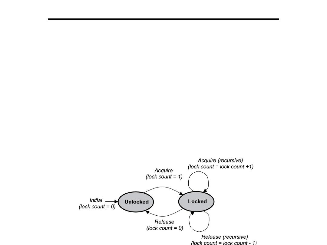
Real-time operating systems
3)Mutual Exclusion (Mutex) Semaphores: A mutual exclusion (mutex) semaphore
is a special binary semaphore that supports ownership, recursive access, task deletion
safety, and one or more protocols for avoiding problems inherent to mutual
exclusion.
As opposed to the available and unavailable states in binary and counting
semaphores, the states of a mutex are unlocked or locked (0 or 1, respectively). A
mutex is initially created in the unlocked state, in which it can be acquired by a task.
After being acquired, the mutex moves to the locked state. Conversely, when the task
releases the mutex, the mutex returns to the unlocked state. Note that some kernels
might use the terms lock and unlock for a mutex instead of acquire and release.
Depending on the implementation, a mutex can support additional features not found
in binary or counting semaphores. These key differentiating features include
ownership, recursive locking, task deletion safety, and priority inversion avoidance
protocols.
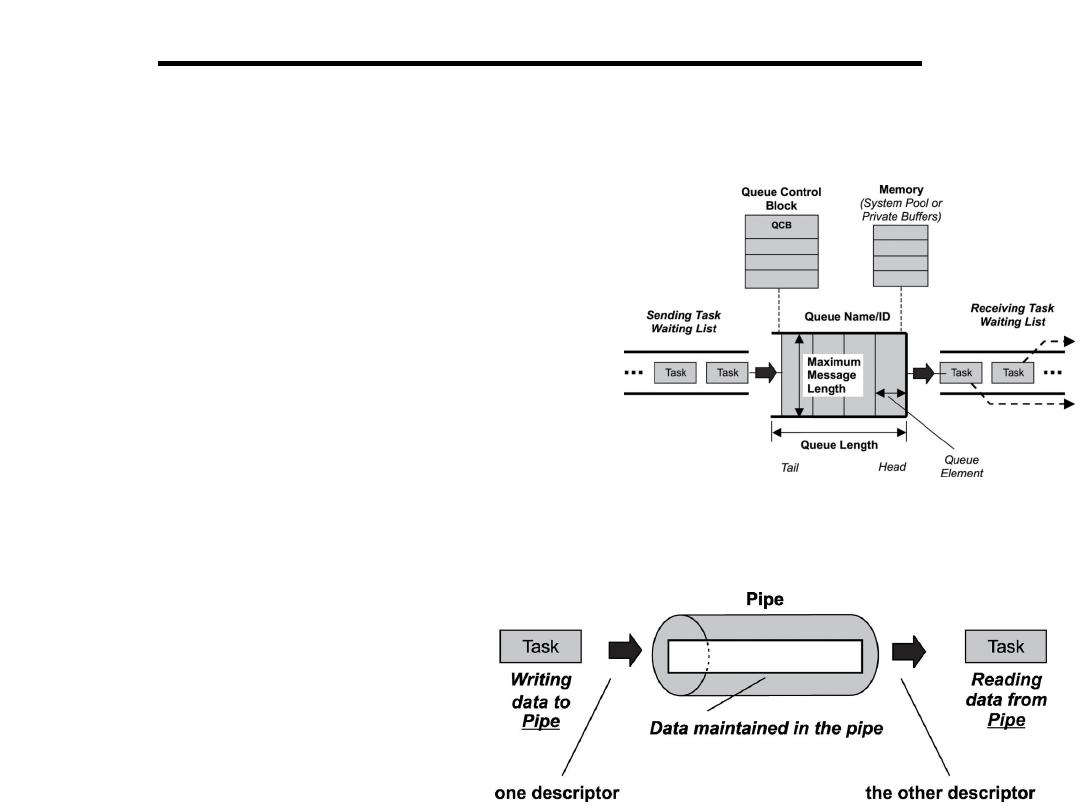
Real-time operating systems
•Message Queues: A message queue is a buffer-like object through which tasks and
ISRs send and receive messages to communicate and synchronize with data. A
message queue is like a pipeline. It temporarily holds messages from a sender until
the intended receiver is ready to read them.
This temporary buffering decouples a sending and
receiving task; that is, it frees the tasks from having
to send and receive messages simultaneously.
•Pipes: Pipes are kernel objects that provide
unstructured data exchange and facilitate
synchronization among tasks.
In a traditional implementation, a pipe is a unidirectional data exchange facility. Two
descriptors, one for each end of the pipe (one end for reading and one for writing),
are returned when the pipe is created. Data is written via one descriptor and read via
the other.
The data remains in the pipe as an
unstructured byte stream. Data is read
from the pipe in FIFO order.
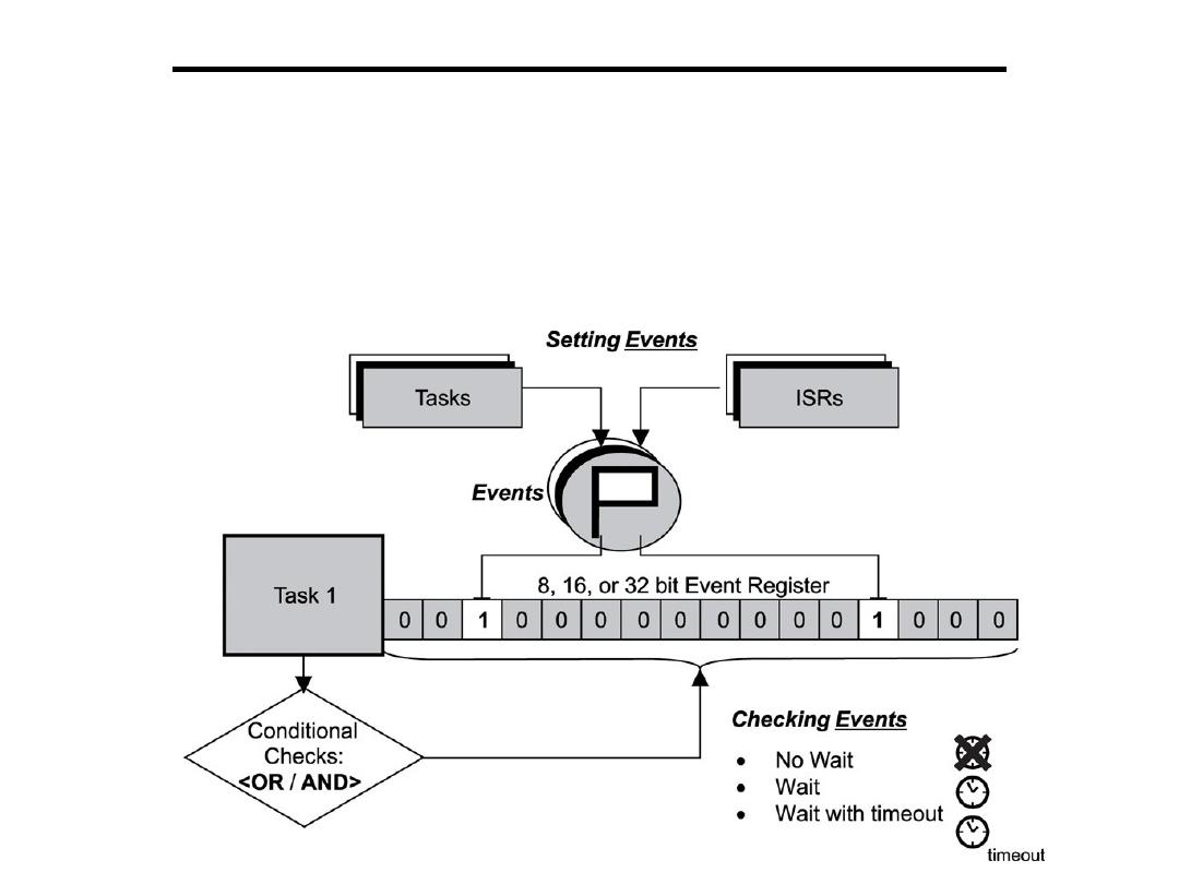
Real-time operating systems
•Event Registers: Some kernels provide a special register as part of each task’s
control block. This register, called an event register, is an object belonging to a task
and consists of a group of binary event flags used to track the occurrence of specific
events. Through the event register, a task can check for the presence of particular
events that can control its execution. An external source, such as another task or an
interrupt service routines (ISR), can set bits in the event register to inform the task
that a particular event has occurred.
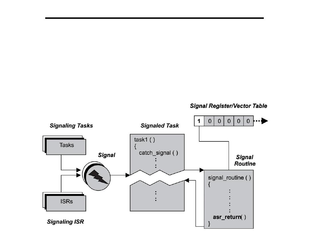
Real-time operating systems
•Signals: A signal is a software interrupt that is generated when an event has
occurred. It diverts the signal receiver from its normal execution path and triggers the
associated asynchronous processing. Essentially, signals notify tasks of events that
occurred during the execution of other tasks or (interrupt service routines) ISRs. As
with normal interrupts, these events are asynchronous to the notified task and do not
occur at any predetermined point in the task’s execution. The difference between a
signal and a normal interrupt is that signals are so-called software interrupts, which
are generated via the execution of some software within the system.
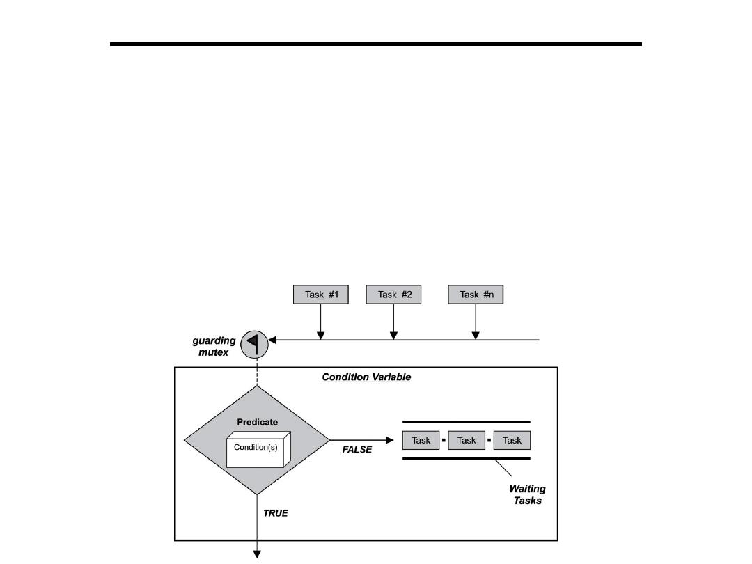
Real-time operating systems
•Condition Variables: Tasks often use shared resources, such as files and
communication channels. When a task needs to use such a resource, it might need to
wait for the resource to be in a particular state. The way the resource reaches that
state can be through the action of another task. In such a scenario, a task needs some
way to determine the condition of the resource. One way for tasks to communicate
and determine the condition of a shared resource is through a condition variable. A
condition variable is a kernel object that is associated with a shared resource, which
allows one task to wait for other task(s) to create a desired condition in the shared
resource. A condition variable can be associated with multiple conditions

Real-time operating systems
•Timers: Timers are used to measure the elapsed time of events. For instant, the
kernel has to keep track of different times:
–A particular task may need to be executed periodically, say, every 10 msec. A timer
is used to keep track of this periodicity
–A task may be waiting in a queue for an event to occur. If the event does not occur
for a specified time, it has to take appropriate action.
–A task may be waiting in a queue for a shared resource. If the resource is not
available for a specified time, an appropriate action has to be taken.
•Foreground/Background Systems:
Small systems of low complexity are generally designed as shown in Figure. These
systems are called foreground/background or super-loops. An application consists of
an infinite loop that calls modules (that is, functions) to perform the desired
operations (background). Interrupt Service Routines (ISRs) handle asynchronous
events (foreground). Foreground is also called interrupt level while background is
called task level. Critical operations must be performed by the ISRs to ensure that
they are dealt with in a timely fashion. Because of this, ISRs have a tendency to take
longer than they should. Also, information for a background module made available
by an ISR is not processed until the background routine gets its turn to execute. This
is called the task level response.
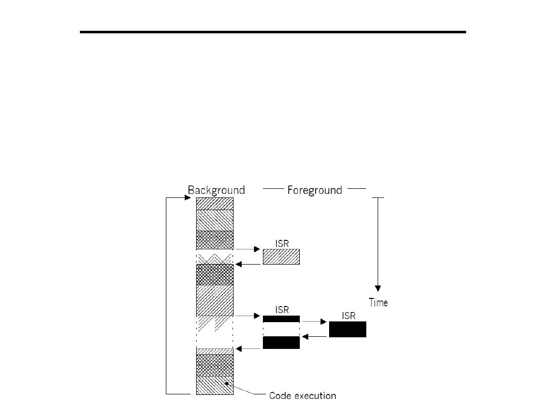
Real-time operating systems
The worst case task level response time depends on how long the background loop
takes to execute. Because the execution time of typical code is not constant, the time
for successive passes through a portion of the loop is non-deterministic.
Furthermore, if a code change is made, the timing of the loop is affected. Most high
volume microcontroller-based applications (e.g., microwave ovens, telephones, toys,
and so on) are designed as foreground/background systems. Also, in
microcontroller-based applications, it may be better (from a power consumption
point of view) to halt the processor and perform all of the processing in ISRs.

Real-time operating systems
•Spooling(Simultaneous Peripheral Operation On-Line) : Print
resources are shared between active programs, Printouts are generated
in pieces as the CPU gives each concurrent program some time
Problem:
•The current program may generate a few print lines
•The CPU moves to the next program
•The second program may generate a few print lines, etc.
Result:
•Printout is worthless as it contains a few lines from several programs
Solution – Spooling
•Each program thinks it is writing to the printer
•The program actually writes to the hard disk
•When the program is complete, the file on the hard disk is sent to the
printer

Real-time operating systems
•Spooling means that each program writes onto a disk each file that is
to be printed.
•Although the program thinks it is writing to the printer, the operating
system intercepts that output and sends it instead to the disk.
•When the entire file is on the disk, spooling is complete, and the disk
files are printed intact.
•Spooling to disk is much faster than writing that same record on a
printer. A program, therefore, completes execution more quickly if
records to be printed are written temporarily on disk instead.
•Spooling overlaps the I/O of one job with the computation of other
jobs.
•The spooler may be reading the input of one job while printing the
output of a different job.
•By overlaps, spooling keeps both the CPU and the I/O devices
working at much higher rates.

The Scheduler
The scheduler is at the heart of every kernel. A scheduler provides the
algorithms needed to determine which task executes when. To understand how
scheduling works, this section describes the following topics:
1)Schedulable entities,
2)Multitasking,
3)Context switching,
4)Dispatcher
5)Scheduling algorithms
•Schedulable Entities:
A schedulable entity is a kernel object that can compete
for execution time on a system, based on a predefined scheduling algorithm. Tasks and
processes are all examples of schedulable entities found in most kernels.
A task is an independent thread of execution that contains a sequence of independently
schedulable instructions. Some kernels provide another type of a schedulable object
called a process. Processes are similar to tasks in that they can independently compete
for CPU execution time. Processes differ from tasks in that they provide better memory
protection features, at the expense of performance and memory overhead. Despite these
differences, for the sake of simplicity, this book uses task to mean either a task or a
process.
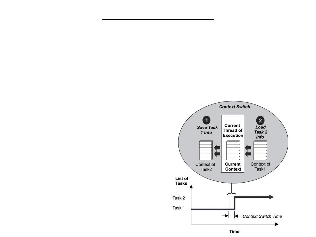
The Scheduler
•Multitasking: Multitasking is the ability of the operating system to handle
multiple activities within set deadlines. A real-time kernel might have multiple
tasks that it has to schedule to run. One such multitasking scenario is illustrated
in Figure. In this scenario, the kernel multitasks in such a way that many
threads of execution appear to be running concurrently; however, the kernel is
actually interleaving executions sequentially, based on a preset scheduling
algorithm. The scheduler must ensure that the appropriate task runs at the right
time.
An important point to note here is
that the tasks follow the kernel’s
scheduling algorithm, while interrupt
service routines (ISR) are triggered
to run because of hardware interrupts
and their established priorities.

The Scheduler
•The Context Switch: Each task has its own context, which is the state of the CPU
registers required each time it is scheduled to run. A context switch occurs when
the scheduler switches from one task to another. To better understand what
happens during a context switch, let’s examine further what a typical kernel does in
this scenario.
Every time a new task is created, the kernel also creates and maintains an
associated task control block (TCB). TCBs are system data structures that the
kernel uses to maintain task-specific information. TCBs contain everything a
kernel needs to know about a particular task. When a task is running, its context is
highly dynamic. This dynamic context is maintained in the TCB. When the task is
not running, its context is frozen within the TCB, to be restored the next time the
task runs. A typical context switch scenario is illustrated in the previous Figure
As shown in the previous Figure, when the kernel’s scheduler determines that it
needs to stop running task 1 and start running task 2, it takes the following steps:
1)The kernel saves task 1’s context information in its TCB. 2)It loads task 2’s
context information from its TCB, which becomes the current thread of execution.
3)The context of task 1 is frozen while task 2 executes, but if the scheduler needs
to run task 1 again, task 1 continues from where it left off just before the context
switch.

The Scheduler
•The Dispatcher: The dispatcher is the part of the scheduler
that performs context switching and changes the flow of
execution. At any time an RTOS is running, the flow of
execution, also known as flow of control, is passing through
one of three areas: through an application task, through an
ISR, or through the kernel. When a task or ISR makes a
system call, the flow of control passes to the kernel to execute
one of the system routines provided by the kernel. When it is
time to leave the kernel, the dispatcher is responsible for
passing control to one of the tasks in the user’s application. It
will not necessarily be the same task that made the system call.
It is the scheduling algorithms (to be discussed later) of the
scheduler that determines which task executes next. It is the
dispatcher that does the actual work of context switching and
passing execution control.

The Scheduler
Depending on how the kernel is first entered, dispatching can
happen differently. When a task makes system calls, the
dispatcher is used to exit the kernel after every system call
completes. In this case, the dispatcher is used on a call-by-call
basis so that it can coordinate task-state transitions that any of
the system calls might have caused. (One or more tasks may
have become ready to run, for example.)
On the other hand, if an ISR makes system calls, the dispatcher
is bypassed until the ISR fully completes its execution. This
process is true even if some resources have been freed that
would normally trigger a context switch between tasks. These
context switches do not take place because the ISR must
complete without being interrupted by tasks. After the ISR
completes execution, the kernel exits through the dispatcher so
that it can then dispatch the correct task.

Real-Time Tasks
•Periodic tasks
- Time-driven. Characteristics are known a priori
- Task T
i
is characterized by (p
i
, c
i
)
E.g.: Task monitoring temperature of a patient in an ICU.
•Aperiodic tasks
- Event-driven. Characteristics are not known a priori
- Task T
i
is characterized by (a
i
, r
i
, c
i
, d
i
)
E.g.: Task activated upon detecting change in patient’s condition.
•Sporadic Tasks
– Aperiodic tasks with known minimum inter-arrival time.
p
i
: task period a
i
: arrival time r
i
: ready time
d
i
: deadline c
i
: worst case execution time.
•Task constraints
–Deadline constraint
–Resource constraints
1)Shared access (read-read). 2)Exclusive access (write-x)
–Precedence constraints
T1 T2: Task T2 can start executing only after T1 finishes its execution
–Fault-tolerant Requirements
1)To achieve higher reliability for task execution. 2)Redundancy in execution

Concept of Predictability
• The most common denominator that is expected from a real-
time system is predictability.
– The behavior of the real-time system must be
predictable which means that with certain
assumptions about workload and failures, it
should be possible to show at “design time”
that all the timing constraints of the
application will be met.
• For static systems, 100% guarantees can be given at design
time.
• For dynamic systems, 100% guarantee cannot be given since
the characteristics of tasks are not known a priori.
• In dynamic systems, predictability means that once a task is
admitted into the system, its guarantee should never be
violated as long as the assumptions under which the task was
admitted hold.
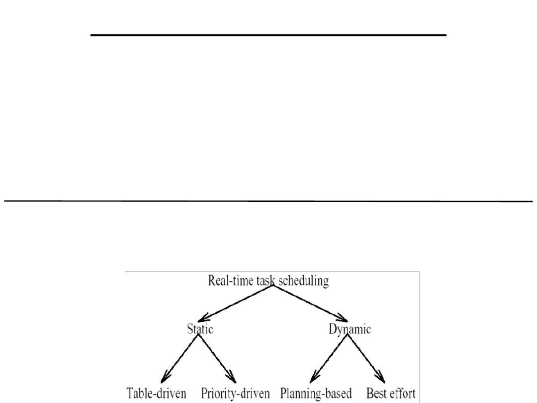
Real-Time Systems - Issues
1) Resource Management (RM) Issues
– Scheduling, Fault-tolerance, Resource reclaiming, Communication
2) Architectural Issues
– Computing subsystem, Communication subsystem, I/O subsystem
3) Software Issues
– Requirements, specification, and verification, Real-time languages, Real-time
databases
Real-time Scheduling Paradigms – RM Issue
Allocate time slots for tasks onto processor(s)[i.e., Where and When a given
task executes]. The objective is: predictably meeting task deadlines.

Preemptive vs. Non-preemptive scheduling
•Preemptive Scheduling
– Task execution is preempted and resumed later
– Preemption occurs to execute higher priority task.
– Offers higher schedulability
– Involves higher scheduling overhead due to context switching
•Non-preemptive Scheduling
– Once a task starts executing, it completes its full execution
– Offers lower schedulability
– Less overhead due to less context switching
Optimal scheduling – definition:
– A static scheduling algorithm is said to be optimal if, for any set of tasks, it
always produces a feasible schedule (i.e., a schedule that satisfies the constraints
of the tasks) whenever any other algorithm can do so.
– A dynamic scheduling algorithm is said to be optimal if it always produces a
feasible schedule whenever a static algorithm with complete prior knowledge of
all the possible tasks can do so.
– Static scheduling is used for scheduling periodic tasks, whereas dynamic
scheduling is used to schedule both periodic and aperiodic tasks.

Real-Time Systems - Issues
Architectural Issues:
• Predictability in: Instruction execution time, Memory access, Context
switching, Interrupt handling.
• RT systems usually avoid caches and superscalar features.
• Support for error handling (self-checking circuitry, voters, system
monitors).
• Support for fast and reliable communication (routing, priority
handling, buffer and timer management).
• Support for scheduling algorithms (fast preemptability, priority
queues).
• Support for RTOS (multiple contexts, memory management, garbage
collection, interrupt handling, clock synchronization).
• Support for RT language features (language constructs for estimating
worst-case execution time of tasks).
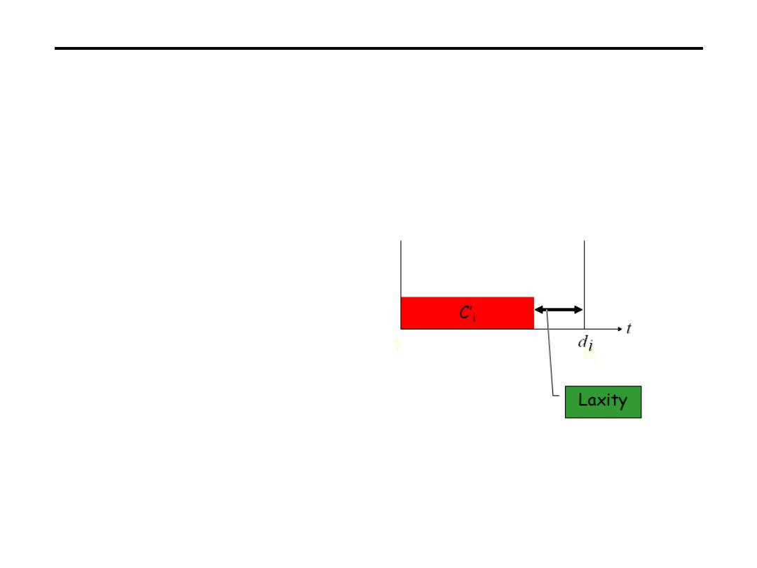
Priority-driven Preemptive Scheduling
Assumptions & Definitions
• Tasks are periodic
• No aperiodic or sporadic tasks
• Job (instance) deadline = end of period
• No resource constraints
• Tasks are preemptable
• Laxity of a Task
Ti = d
i
– (t + c
i
’)
where
di: deadline;
t : current time;
c
i
’ : remaining computation time.
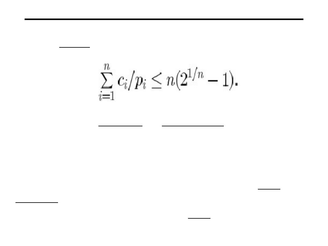
Rate Monotonic Scheduling (RMS)
• Schedulability check (off-line):
- A set of n tasks is schedulable on a uniprocessor by the RMS
algorithm if the processor utilization (utilization test):
The term n(2
1/n
-1) approaches ln 2, (
≈
0.69 as n
→
∞
).
- This condition is sufficient, but not necessary.
• Schedule construction (online)
- Task with the smallest period is assigned the highest priority.
- At any time, the highest priority task is executed.
RMS is an optimal preemptive scheduling algorithm with fixed
priorities.
Static/fixed priority algorithm assigns the same priority to all the jobs
(instances) in each task.
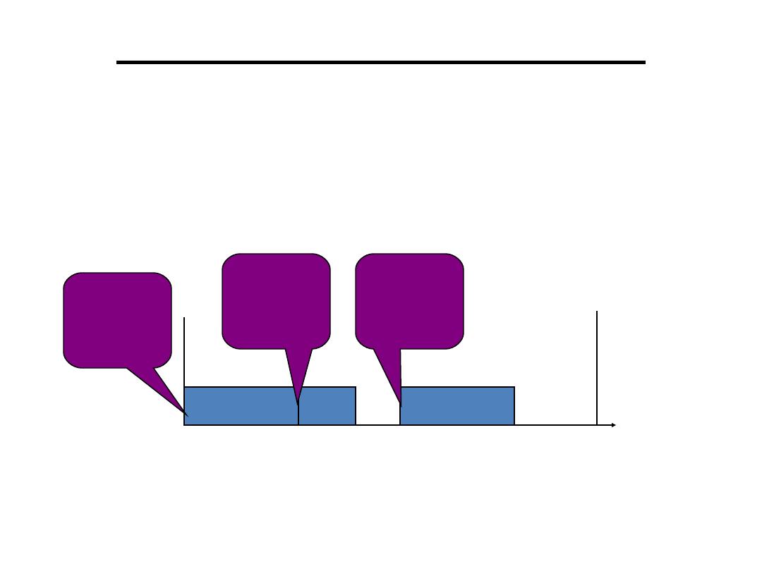
RMS Scheduler -- Example 1
Task set: T
i
= (c
i
, p
i
)
T1 = (2,4) and T2 = (1,8)
Schedulability check:
2/4 + 1/8 = 0.5 + 0.125 = 0.625 ≤ 2(√2 -1) = 0. 82
T
1
1
T
2
1
T
1
2
0
2
3
4
6
8
Active
Tasks
:
{
T1, T2
}
Active
Tasks
:
{
T2
}
Active
Tasks
:
{
T1
}
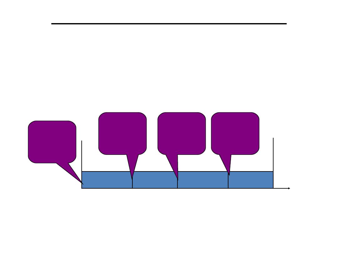
RMS scheduler -- Example-2
Task set: T
i
= (c
i
, p
i
)
T1 = (2,4) and T2 = (4,8)
Schedulability check:
2/4 + 4/8 = 0.5 + 0.5 = 1.0 > 2(√2 -1) = 0. 82
T
1
1
T
2
1
T
1
2
0
2
3
4
6
8
Active
Tasks
:
{
T1, T2
}
Active
Tasks
:
{
T2
}
Active
Tasks
:
{
T2, T1
}
T
2
1
Active
Tasks
:
{
T2
}
Some task sets that FAIL the utilization-based schedulability
test are also schedulable under RMS We need exact
analysis (necessary & sufficient)
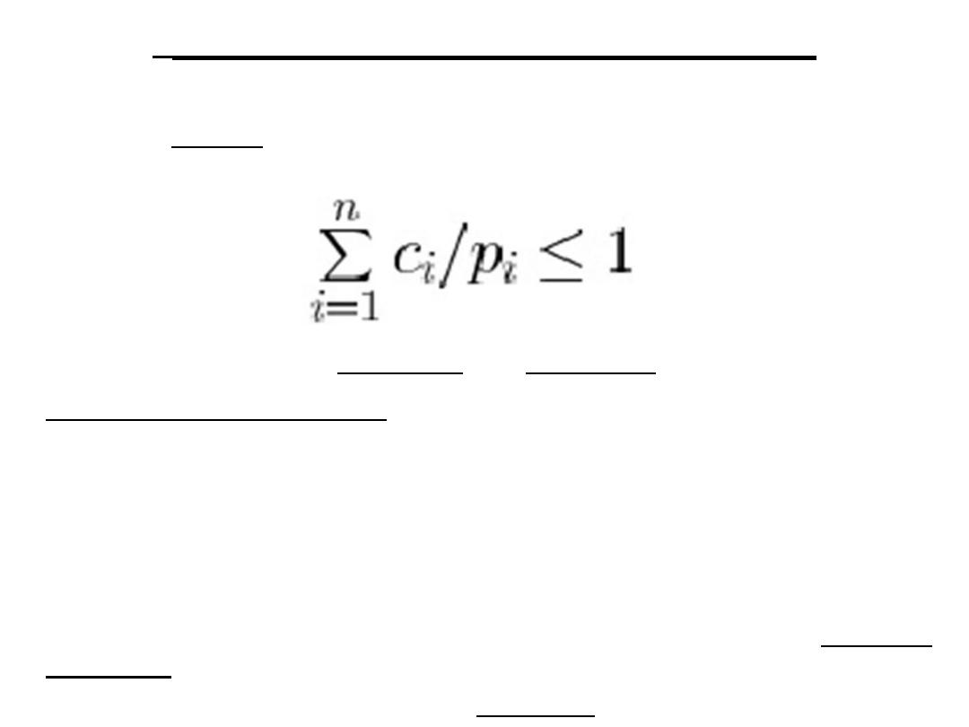
Earliest Deadline First (EDF
)
• Schedulability check (off-line)
- A set of n tasks is schedulable on a uniprocessor by the EDF
algorithm if the processor utilization.
• This condition is both necessary and sufficient.
- Least Laxity First (LLF) algorithm has the same schedulability
check.
• Schedule construction (online)
– EDF/LLF: Task with the smallest deadline/laxity is assigned the
highest priority.
– At any time, the highest priority task is executed.
EDF/LLF is an optimal preemptive scheduling algorithm with dynamic
priorities.
Dynamic priority algorithm assigns different priorities to the individual
jobs (instances) in each task.
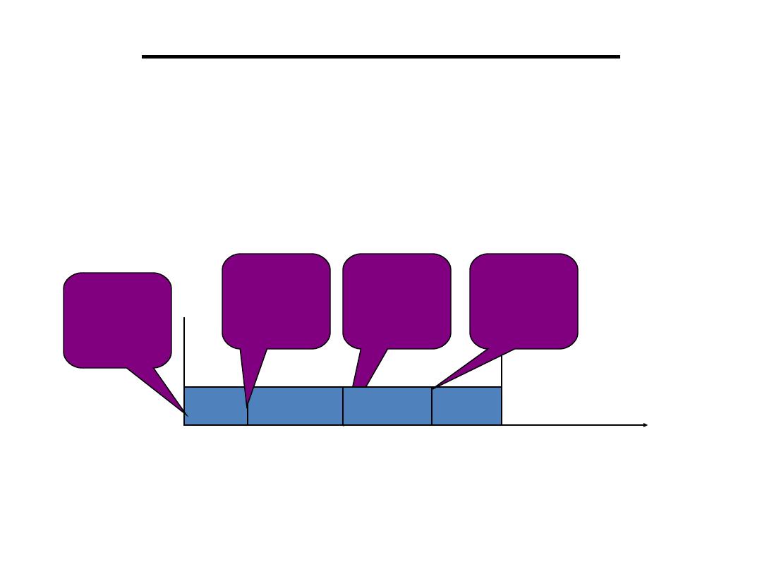
EDF scheduler -- Example
Task set: T
i
= (c
i
, p
i
, d
i
)
T1 = (1,3,3) and T2 = (4,6,6)
Schedulability check:
1/3 + 4/6 = 0.33 + 0.67 = 1.0
T
1
1
T
2
1
T
1
2
0
1
5
6
Active
Tasks
:
{
T1, T2
}
Active
Tasks
:
{
T2
}
Active
Tasks
:
{
T2, T1
}
Active
Tasks
:
{
T1
}
Unlike RMS, Only those task sets which pass the schedulability
test are schedulable under EDF
3
T
2
1

RMS vs. EDF/LLF
• RMS is an optimal preemptive scheduling algorithm
with fixed priorities.
• EDF/LLF is an optimal preemptive scheduling
algorithm with dynamic priorities.
• RMS schedulability properties can be analyzed; rich
theory exists and it is widely used in practice.
• EDF/LLF offers higher schedulability than RMS, but
it is more difficult to implement.
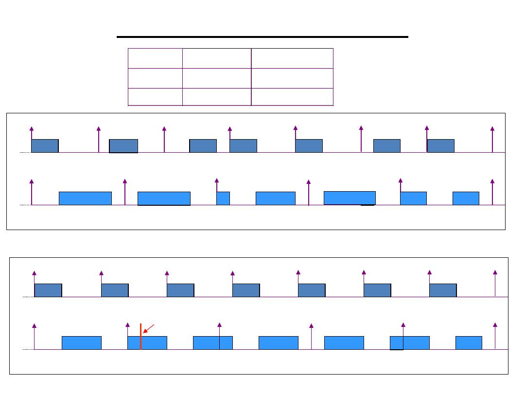
RMS & EDF -- Example
0
5
10
15
20
25
30
35
0
7
14
21
28
35
T
1
T
2
RMS schedule
0
5
10
15
20
25
30
35
0
7
14
21
28
35
T
1
T
2
EDF schedule
Deadline miss
Process
Period
,
T
WCET
,
Ca
T
1
5
2
T
2
7
4

Priority Inversion Problem
Priority inversion is an undesirable situation in which a higher priority
task gets blocked (waits for CPU) for more time than that it is supposed
to, by lower priority tasks. For example:
•Let T
1
, T
2
, and T
3
be the three periodic tasks with decreasing order of
priorities.
•Let T
1
and T
3
share a resource “S”. T3 obtains a lock on the semaphore
S and enters its critical section to use a shared resource.
•T1 becomes ready to run and preempts T3. Then, T1 tries to enter its
critical section by first trying to lock S. But, S is already locked by T3
and hence T1 is blocked.
•T2 becomes ready to run. Since only T2 and T3 are ready to run, T2
preempts T3 while T3 is in its critical section.
•Ideally, one would prefer that the highest priority task (T1) be blocked
no longer than the time for T3 to complete its critical section. However,
the duration of blocking is, in fact, unpredictable because task T2 got
executed in between.
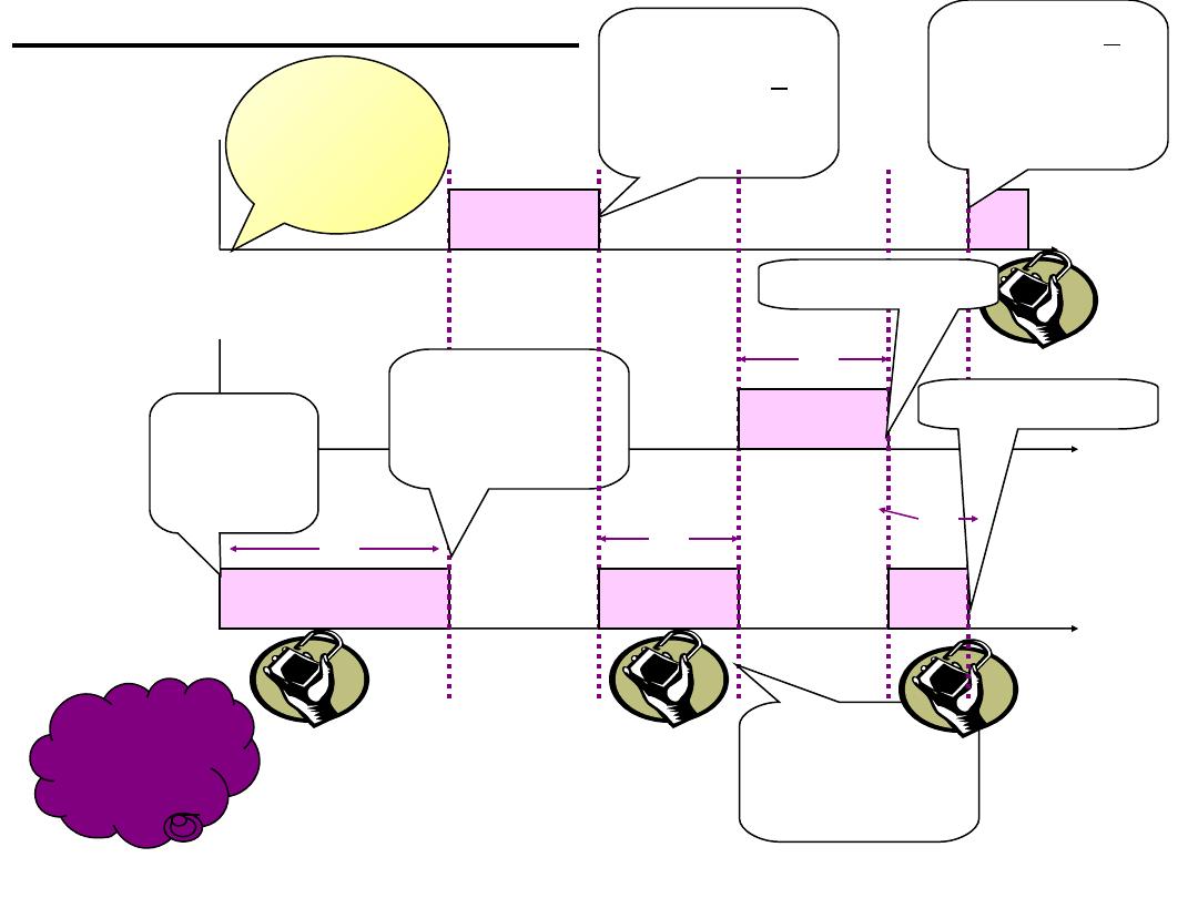
Priority Inversion example
T1
T2
T
3
T3
0
T3 is the
only
active task
Preempted by
higher priority
task T1
T
1
Makes a request
for resource S
and gets
blocked
T
3
Preempted by
higher priority
task T2
T
2
T
3
T3 completes
T
1
Resource S is
available and
T1 is scheduled
here
K
1
K
2
K
3
T2 completes
L1
Total blocking time for task T1 = (K1+K2+K3) + (L1
)
Highest
priority
Least
priority
Medium
priority
T1 and T3
share
resource S
A higher
priority task
waits for a
lower priority
task
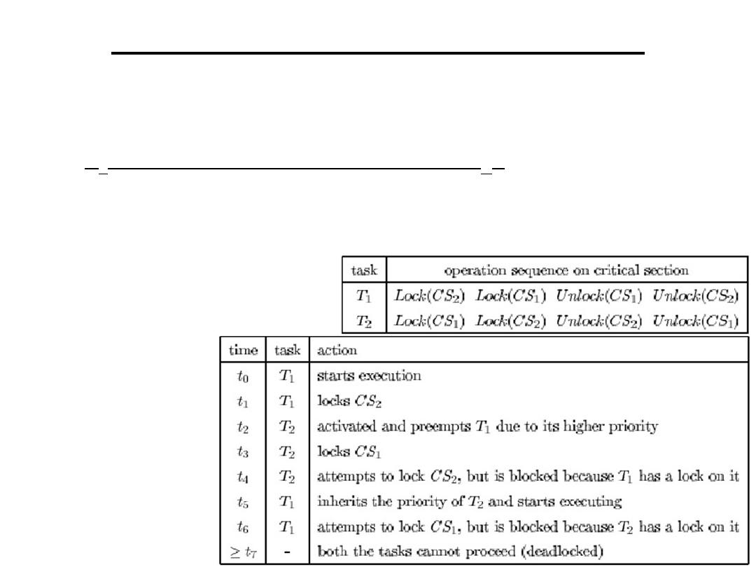
Priority Inheritance Protocol
•Priority inheritance protocol solves the problem of priority inversion.
•Under this protocol, if a higher priority task T
H
is blocked by a lower
priority task T
L
, because T
L
is currently executing critical section needed
by T
H
, T
L
temporarily inherits the priority of T
H
.
•When blocking ceases (i.e., T
L
exits the critical section), T
L
resumes its
original priority.
•Unfortunately, priority inheritance may lead to deadlock.
•T2 has high priority

Priority Ceiling Protocol
• Priority ceiling protocol solves the priority inversion
problem without getting into deadlock.
• For each semaphore, a priority ceiling is defined, whose
value is the highest priority of all the tasks that may lock it.
• When a task T
i
attempts to execute one of its critical
sections, it will be suspended unless its priority is higher
than the priority ceiling of all semaphores currently locked
by tasks other than T
i
.
• If task Ti is unable to enter its critical section for this
reason, the task that holds the lock on the semaphore with
the highest priority ceiling is said to be blocking Ti and
hence inherits the priority of Ti.
As long as a task Ti is not attempting to enter one of its critical
sections, it will preempt every task that has a lower priority.

Priority Ceiling Protocol -- properties
• This protocol is the same as the priority inheritance protocol,
except that a task T
i
can also be blocked from entering a
critical section if any other task is currently holding a
semaphore whose priority ceiling is greater than or equal to
the priority of task T
i
.
• Prevents mutual deadlock among tasks
• A task can be blocked by lower priority tasks at most once
• For the previous example, the priority ceiling for both CS1
and CS2 is the priority of T2.
• From time t0 to t2, the operations are the same as before.
• At time t3, T2 attempts to lock CS1, but is blocked since CS2
(which has been locked by T1) has a priority ceiling equal to
the priority of T2.
• Thus T1 inherits the priority of T2 and proceeds to
completion, thereby preventing deadlock situation.

Deadlock and Starvation
• Principles of deadlock: Deadlock is the permanent blocking of a set of processes
that either compete for system resources or communicate with each other.
– Types of resources
• Reusable
– A reusable resource is one that can be safely used by only one process
at a time and is not depleted by that use.
– Examples: processors, I/O channels, main and secondary memory,
devices, files, data bases, semaphores
• Consumable
– A consumable resource is one that can be created and destroyed.
– The number of consumable resources is usually unlimited.
– When a resource is acquired by a process, the resource ceases to exist.
– Examples: interrupts, signals, messages, information in I/O buffers
• Resource deadlock (reusable resources)
– Circular wait/deadly hold
• Process A holds resource 1 and is requesting resource 2.
• Process B holds resource 2 and is requesting resource 1.
• Deadlock occurs if each process refuses to free its acquired resources until it
has obtained everything it requests for.
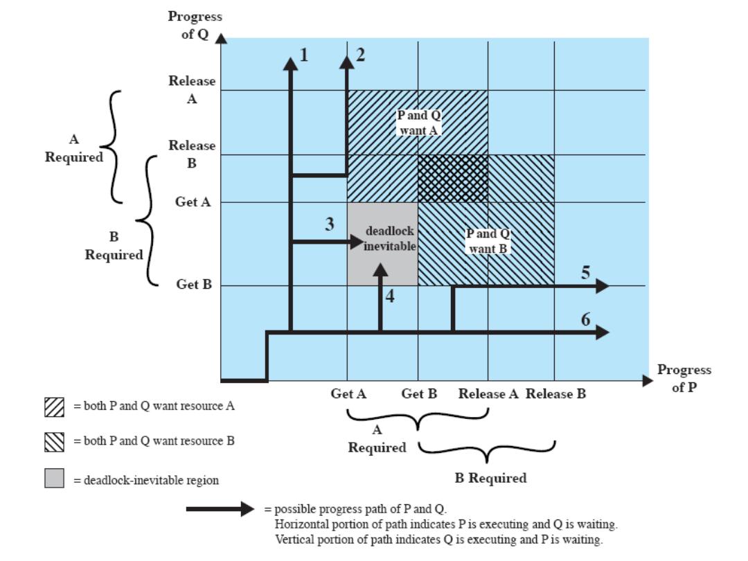
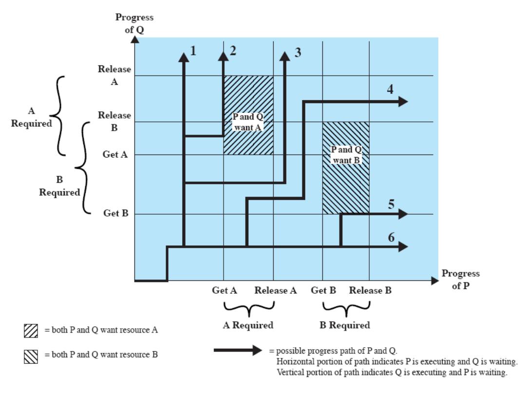

Examples of deadlock
• Deadlock in spooling systems
– In some spooling systems, the complete output from a program
must be available before actual printing can begin.
– Deadlock occurs if several partially completed jobs generating
print lines to spool files fill up the available space.
– If the OS administrator is still in control, he/she can kill some of
the deadlocked processes until sufficient spooling space is
available for the remaining jobs.
• Otherwise, the system must be restarted, so that all jobs are
lost.
– Medication
• Specify more spooling space in the OS, if this number must be
preset.
• OS stops admitting more spooling jobs when a saturation
threshold of spooling space, say 75%, is reached.
• Modern OS starts printing before the spooling files are
completely copied into the disks.
• Dynamic allocation of spooling space
Examples of deadlock
• message deadlock: two processes, each waiting to receive a message from the other
• Suppose a server process and a client process run on two different
machines.
– The server first sends an initialization message to the client, and then waits
for a request from the client.
– The client first waits for the initialization message, and then makes requests.
– If the two machines are of the same speed, and they are started
simultaneously, then the system runs smoothly.
– If, say in a few years, the server is upgraded to a high speed one -- so fast
that after the server’s initialization message arrives at the client, the client is
still in its boot up stage, then the initialization message will be lost.
– Thus, the client is waiting for the initialization message, whereas the server
is waiting for a request message from the client.
– A deadlock now occurs.
– This deadlock is difficult to detect.
P1
…
Receive (P2);
…
Send (P2, M1);
P2
…
Receive (P1);
…
Send (P1, M2);

Starvation
• This is the phenomenon where the scheduling of a process is delayed
indefinitely while other processes receive the attention of the OS.
• also called indefinite blocking or indefinite postponement
• Starvation occurs because of biases in a system’s resource
scheduling policies.
– When resources are scheduled on a priority basis, it is possible
for a given process to wait indefinitely for a resource as processes
with higher priorities continue arriving.
– Medication
• Aging: Allow a process’s priority to increase as it waits for a
resource.

Four Necessary conditions for deadlocks
• Mutual exclusion condition
– Processes claim exclusive control of the resources they require.
• Hold-and-wait condition
– Processes hold resources already allocated to them while waiting for additional
resources.
– The emphasis here is that not all resources requested are allocated at the same
time.
• No preemption condition
– Resources cannot be removed from the processes holding them until the
resources are used to completion.
• Circular wait condition
– A circular chain of processes exists in which each process holds one or more
resources that are requested by the next process in the chain.
• The four conditions are also sufficient for a deadlock to exist.
– Given the first three conditions, a sequence of events may occur that leads to an
unresolvable circular wait.
• The circular wait is unresolvable because of the first three conditions.
– The first three conditions are policies, whereas circular wait is a circumstance
that might occur depending on the sequencing of requests and releases.

Deadlock prevention
To prevent deadlock: removes any possibility of deadlocks occurring, this may result in
poor resource utilization. Following are most frequently used approach
• Strategies for denying necessary conditions (Havender 1968)
– Denying the mutual exclusion condition: This condition cannot be disallowed.
– Denying the hold-and-wait condition
•Each process request all its required resources at once.
•Resources are granted on an all or none basis.
•If the complete set is not available, the process must wait.
•While the process waits, it cannot hold any resources.
•This strategy may cause indefinite postponement since not all the required
resources may become available at once.
– The process could also have started with only some of the resources. Thus
the scheme causes unnecessary delay.
•It leads to waste of resources.
– The process is granted all its requested resources, but it does not need them
all at the same time.
– Medication -- divide a program into several steps that run relatively
independent of one another. Each step controls its own resource allocation.
– The medication gives better resource utilization, but increases design and
execution overhead.

Deadlock prevention (cont.)
– Denying the no-preemption condition
• When a process holding resources is denied a request for additional
resources, that process must release its held resources.
• The removed resources must be requested again.
• When a process releases resources, it may lose all its work to that point.
– Thus this approach applies only to resources whose state can be easily
saved and restored later.
• Indefinite postponement is possible since a process might repeatedly request
and release the same resources.
– In addition, system performance is degraded in performing the request
and release operations.
• Notice that denying the no-preemption condition is different from denying
the hold-and-wait condition.
– In the no-preemption condition, a process requesting 10 resources may
ask for them one by one; as long as each request is fulfilled, the no-
preemption condition is not violated.
– In the no hold-and-wait condition, the same process must request all 10
resources at the same time.

Deadlock prevention (cont.)
– Denying the circular wait condition
• Each resource is uniquely numbered.
• All processes must request resources in a linear ascending order.
• difficulties
– Resource numbers are preassigned during installation.
– Addition of resources may cause problems, probably the modification
of OS system programs.
– Resource numbering usually reflects the normal ordering in which jobs
use the resources. For jobs needing the resources in a different order
than the assumed one, resources early in the line have to be requested
and held idle for a long time, causing considerable waste.
– Application programs may have to be reorganized to optimize for the
linear ordering; this destroys the user transparency of resource
management.
– Deadlock prevention strategies are usually too traditional.

Deadlock detection
•
Deadlock recovery
–
Once deadlock has been detected, some strategy is needed for recovery.
–
The following are possible approaches, in order of increasing sophistication.
1. Abort all deadlocked processes.
2. Back up each deadlocked process to some previously defined checkpoint,
and restart all processes.
– Rollback mechanisms are needed.
– After restarting, due to the nondeterminancy of concurrent processing,
the original deadlock is unlikely to reoccur.
1. Successively abort deadlocked processes until deadlock no longer exists.
– The order of abortion should be based on minimum cost.
– After each abortion, reinvoke the detection algorithm again.
4. Successively preempt resources until deadlock no longer exists.
– The order of preemption is based on minimum cost.
– A process that loses a resource must be rolled back to a point before
its acquisition of that resource.
–
For items 3 and 4, the selection criterion could be:1)least amount of processor
time consumed so far. 2)least number of lines of output produced so far.
3)most estimated time remaining. 4)least total resources allocated so far.
5)lowest priority.

Deadlock detection (cont.)
• Difficulties in deadlock recovery
– The priority order may be biased, such as the deadline of a small
insignificant job.
– Many systems have poor facilities for suspending a process indefinitely,
removing it from the system, and resuming it at a later time.
• not even <Ctrl-Z> in UNIX
• Most systems do not have suspension facilities, and the removed
processes are ordinary lost.
• Even if suspension is possible, it involves considerable overhead and the
attention of highly skilled operators.
• Sometimes there is insufficient skilled manpower -- consider a deadlock
involving tens or hundreds of processes.
• Some systems have checkpoint/restart features, with a loss of the work
since the last checkpoint; this still cost considerable effort on the
application developers.
• Real-time processes can simply not be suspended.
• By not limiting resource access, deadlock detection is too liberal in restricting
process actions.

Deadlock avoidance
• Deadlock avoidance imposes less strict conditions than in
deadlock prevention in order to get better resource
utilization.
• All mutual exclusion, hold-wand-wait, and no-preemption
conditions are allowed.
• Careful choices of allocation are made to assure that
deadlock is never reached.
• A decision is made dynamically on whether the current
resource request could potentially lead to a deadlock.
– Do not start a process if its demands might lead to
deadlock.
– Do not grant an incremental resource request to a process
if this allocation will lead to deadlock.

Deadlock avoidance (cont.)
• Dijkstra’s banker’s algorithm (1965)
– The state of the system is the current allocation of resources
to processes.
– A safe state is one in which there is at least one order in
which all processes can be run to completion within a finite
time without resulting in a deadlock. (It is possible to go
from a safe state to an unsafe state.)
– The OS is equivalent to a banker, and job requests are
equivalent to the clients.
– The system grants requests that result in safe states only.
– Unsafe states need not be deadlocked ; there is only a
potential for deadlock. The banker’s algorithm assures that
there is never such a possibility.
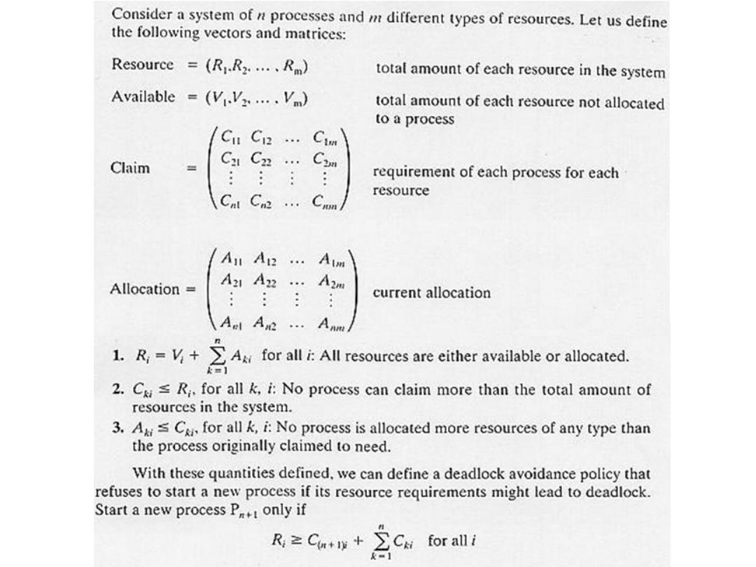
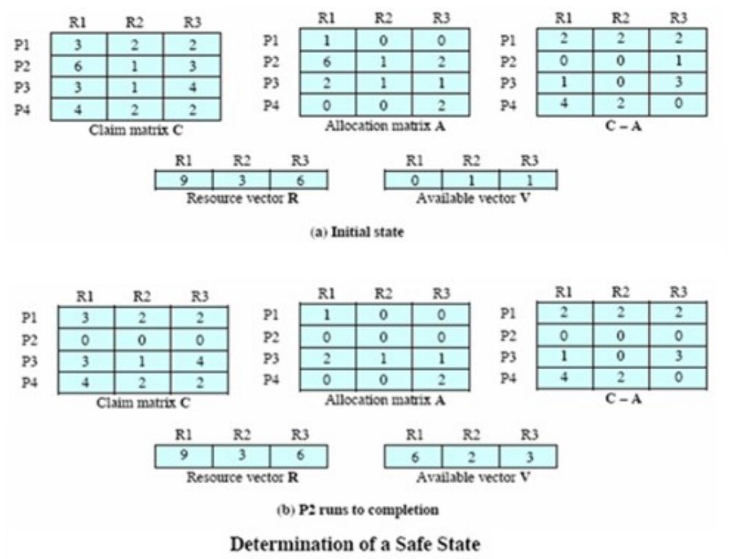
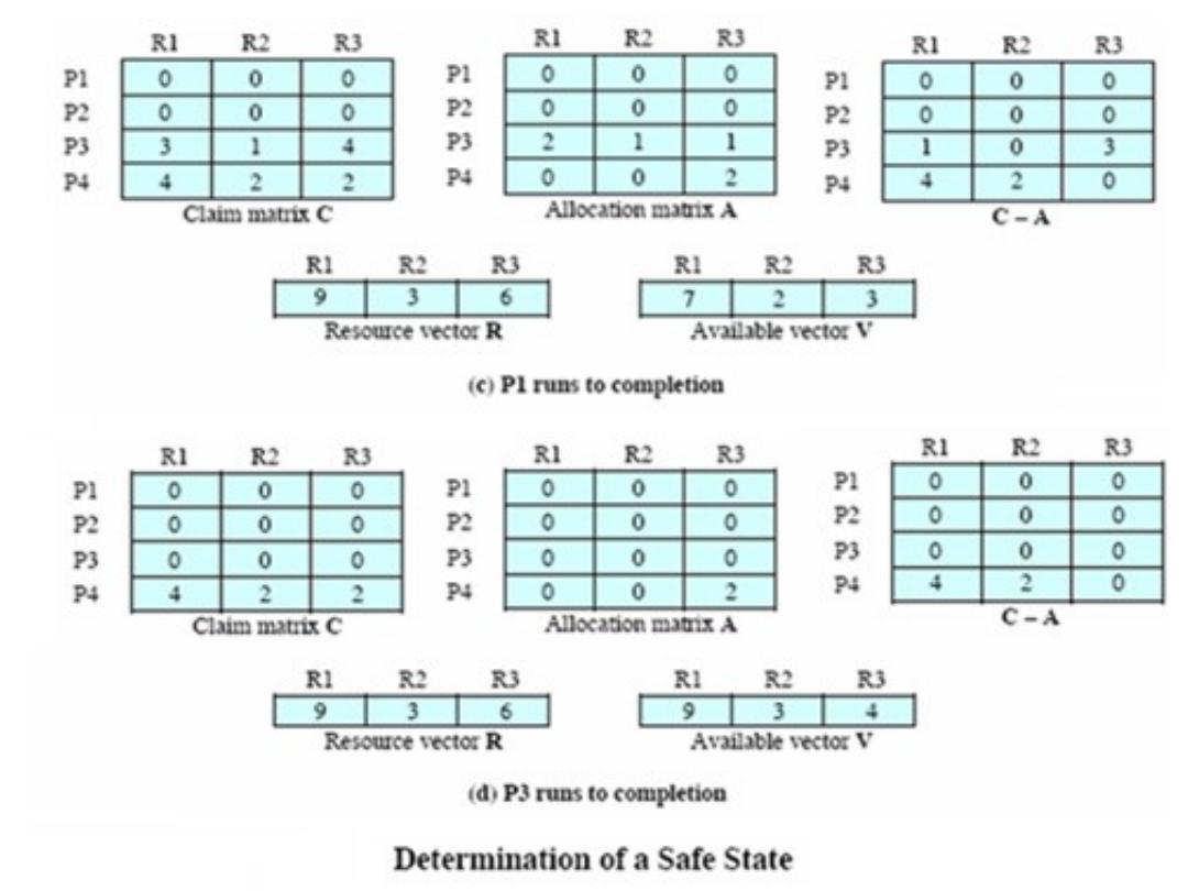
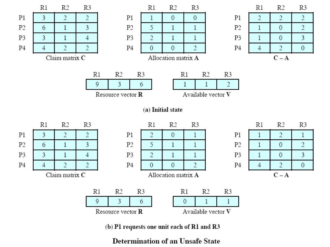

Deadlock avoidance (cont.)
• Weakness in the banker’s algorithm
– The total number of resources available is fixed, but resources
frequently breakdown or require maintenance service.
– The algorithm requires that the banker grant all requests within
a finite time, but “finite time” is insufficient in real-time
systems.
– The algorithm requires that satisfied clients repay all loans
within a finite time, but this may cause lengthy delay to other
clients waiting in line.
– Users must state their maximum resource usage in advance, but
many jobs are interactive and dynamic and users cannot
anticipate their eventual requirements.
– The processes under consideration must be independent -- they
cannot be constrained by any synchronization requirements.

Burglar alarm system
• A system is required to monitor sensors on doors and windows to detect
the presence of intruders in a building.
• When a sensor indicates a break-in, the system switches on lights around
the area and calls police automatically.
• The system should include provision for operation without a mains power
supply.
• Sensors
– Movement detectors, window sensors, door sensors;
– 50 window sensors, 30 door sensors and 200 movement detectors;
– Voltage drop sensor.
• Actions
– When an intruder is detected, police are called automatically;
– Lights are switched on in rooms with active sensors;
– An audible (easy to hear) alarm is switched on;
– The system switches automatically to backup power when a voltage
drop is detected.

The R-T system design process
• Identify stimuli and associated responses.
• Define the timing constraints associated with each stimulus and
response.
• Allocate system functions to concurrent processes.
• Design algorithms for stimulus processing and response generation.
• Design a scheduling system which ensures that processes will always
be scheduled to meet their deadlines.
Stimuli to be processed:
• Power failure
– Generated aperiodically by a circuit monitor. When received, the
system must switch to backup power within 50 ms.
• Intruder alarm
– Stimulus generated by system sensors. Response is to call the
police, switch on building lights and the audible alarm.
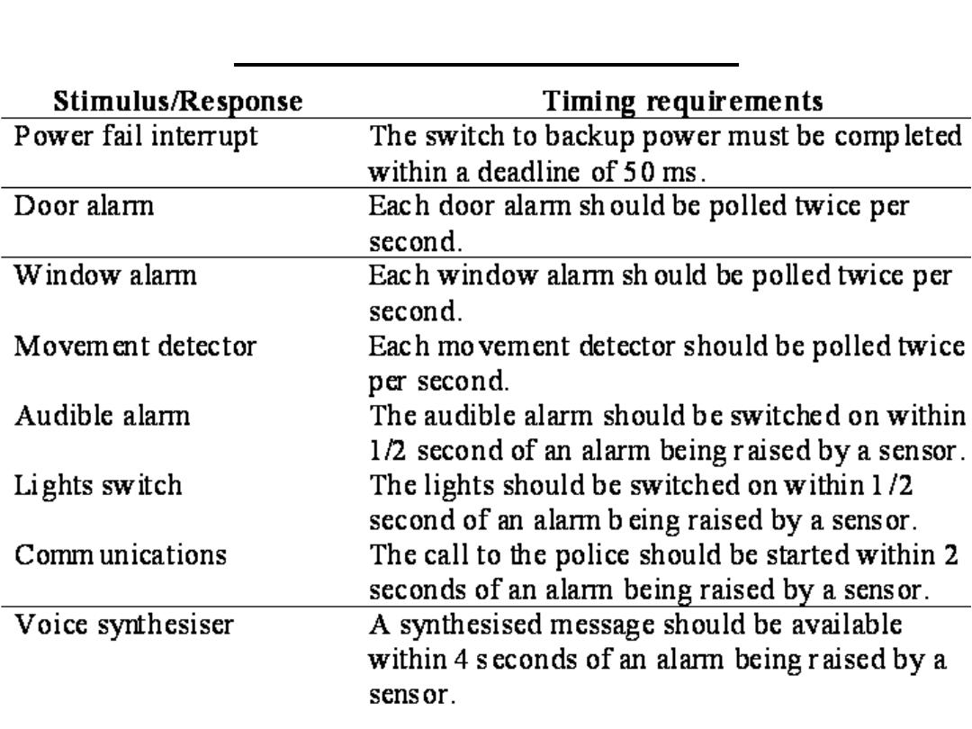
Timing requirements
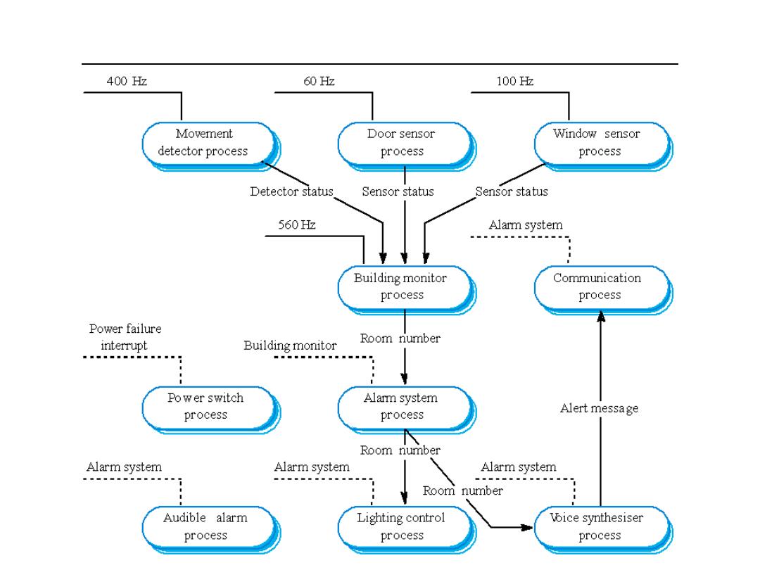
Burglar alarm system processes
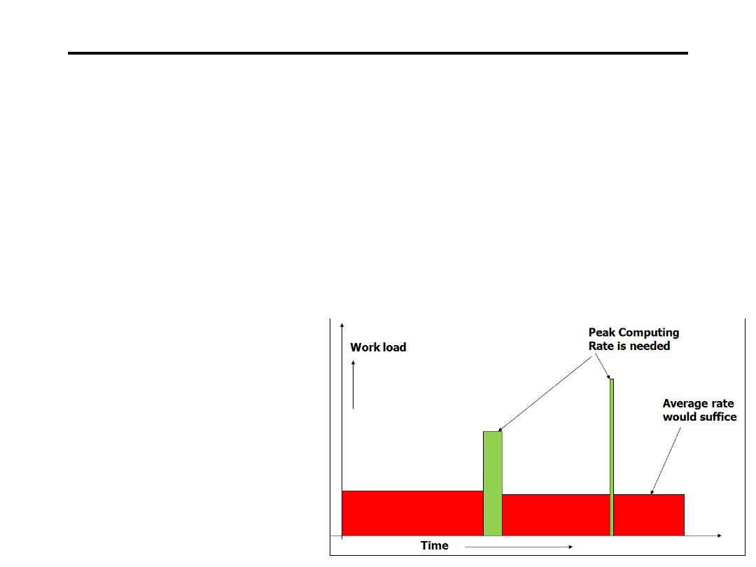
Energy Aware Real Time Systems
•Energy consumption is an important issue in embedded systems.
–Mobile and portable devices: Laptops, PDAs, Mobile and Intelligent systems:
Digital camcorders, cellular phones, and portable medical devices.
•The peak computing rate needed is much higher than the average throughput
that must be sustained;
•High performance is needed only for a small fraction of time, while for the rest
of time, a low-performance, a low-power processor would suffice.
•Processors are based on CMOS logic
•P α V2 . f
•V α f
•Ei = K .cci . f2
•cci = # clock cycles of task Ti.
•f = frequency at which Ti is run.

Variable Voltage Processors
• Modern processors operate at multiple frequency levels:
1. Crusoe Processor: Transmeta Corporation
2. PowerNow! Technology: AMD
3. Intel XScale: Intel
• Higher the frequency level higher the energy consumption
• What is the power consumption of a Crusoe processor?
The extremely low power consumption delivered on multimedia
applications can be directly attributed to a new feature called
LongRun power management. LongRun has the distinct ability to
analyze the application workload dynamically and to adjust
continuously the processor's speed (MHz) and voltage to provide
the necessary performance. This new feature promises to extend the
battery life of all applications, most specifically those requiring the
constant attention of the processor. This is a dramatic departure from
today's ultra-light PCs, which are incapable of delivering over one and
a half or two hours of runtime for DVD movies.
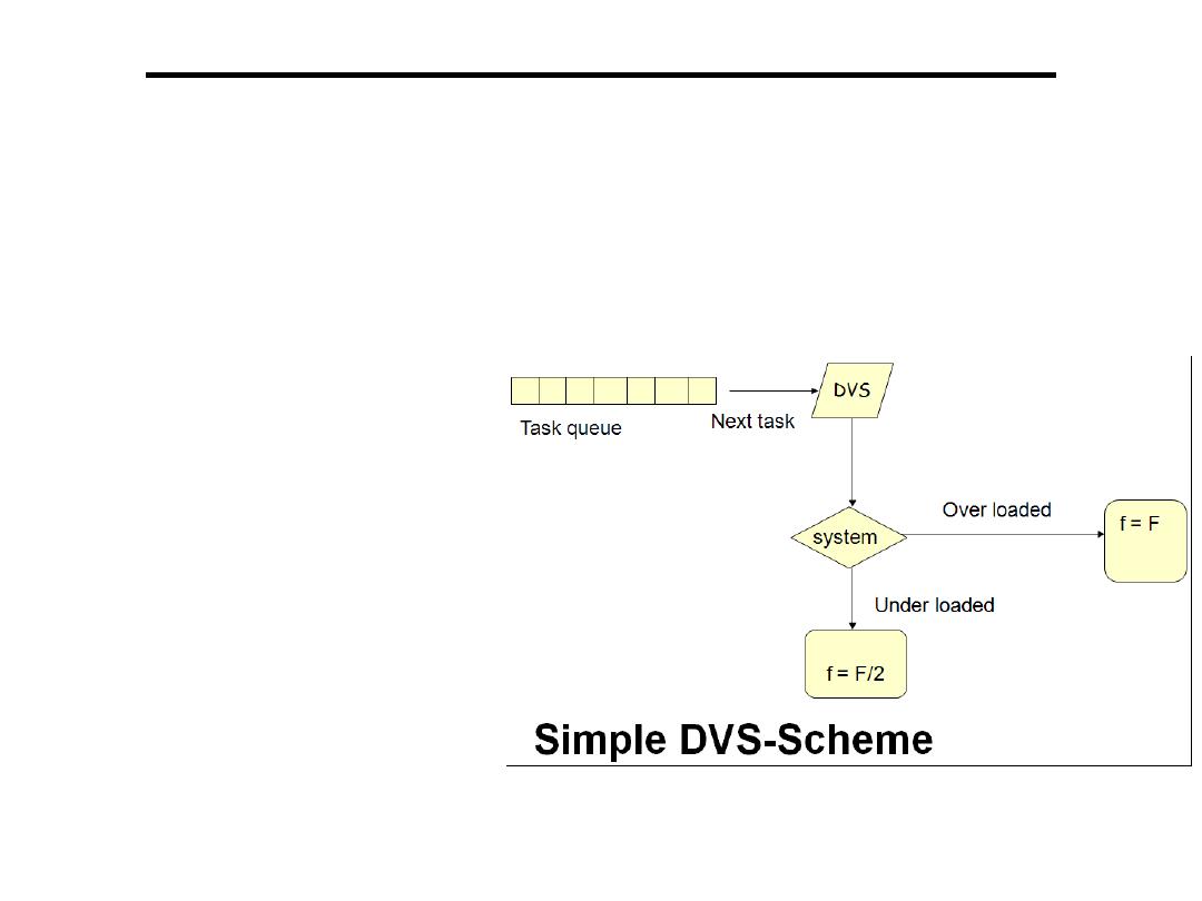
Dynamic Voltage Scaling (DVS)
• DVS scales the operating voltage of the processor along with the
frequency.
• Since energy is proportional to f2 , DVS can potentially provide
significant energy savings through frequency and voltage scaling.
• Consider a task with a computation time 20 units.
• Energy of Ti without DVS:
E1 = K * 20 * F
2
.
• Energy of Ti with DVS:
E2 = K * 20 * (F/2)
2
.
• Clearly, E2 = (E1)/4
• Therefore, if we reduce the frequency we save energy but, we spend
more time in performing the same computation
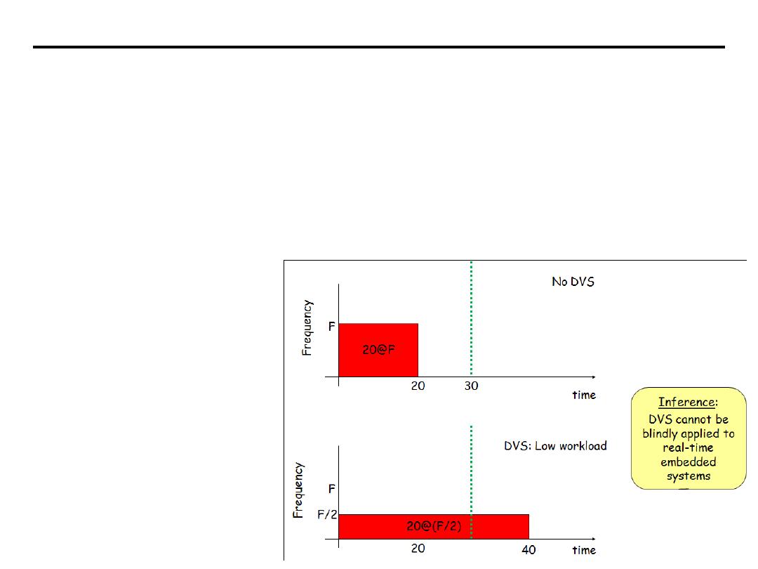
Simple DVS scheme handling RT-task
• Consider a real-time task T1 = (20, 30)
• Applying the simple DVS scheme discussed earlier:
– If there is peak load T1 runs at maximum frequency (F) and meets the
deadline with no energy savings
– It there is less load T1 runs at half the maximum frequency (F/2) and
completes at time = 40 thereby missing its deadline

Energy aware scheduling in RT Systems
• Objectives:
1. Minimizing energy consumption
2. Meeting the deadlines.
• OS Level Energy Management
– The operating voltage/frequency decisions are made at scheduling phase
– The operating voltage is decided at every task release and task completion
– These schemes are also known as Inter-task schemes
• Compiler Level Energy Management
– The operating voltage/frequency decisions are made at the compile time
– The operating voltage is decided at the basic block level
– These schemes are also known as Intra-task schemes
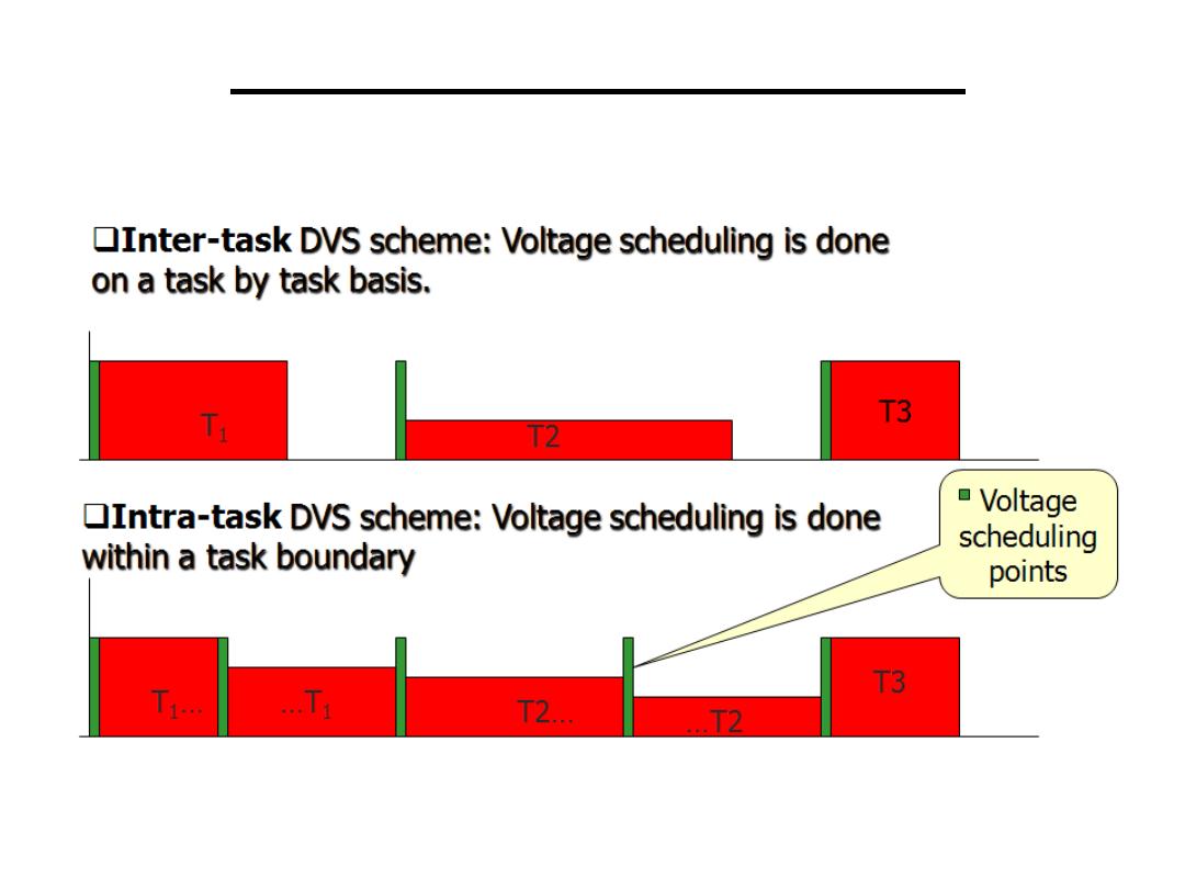
Real Time - DVS schemes
The RT-DVS algorithms can be broadly classified based on the granularity at which
voltage scheduling is performed as follows:
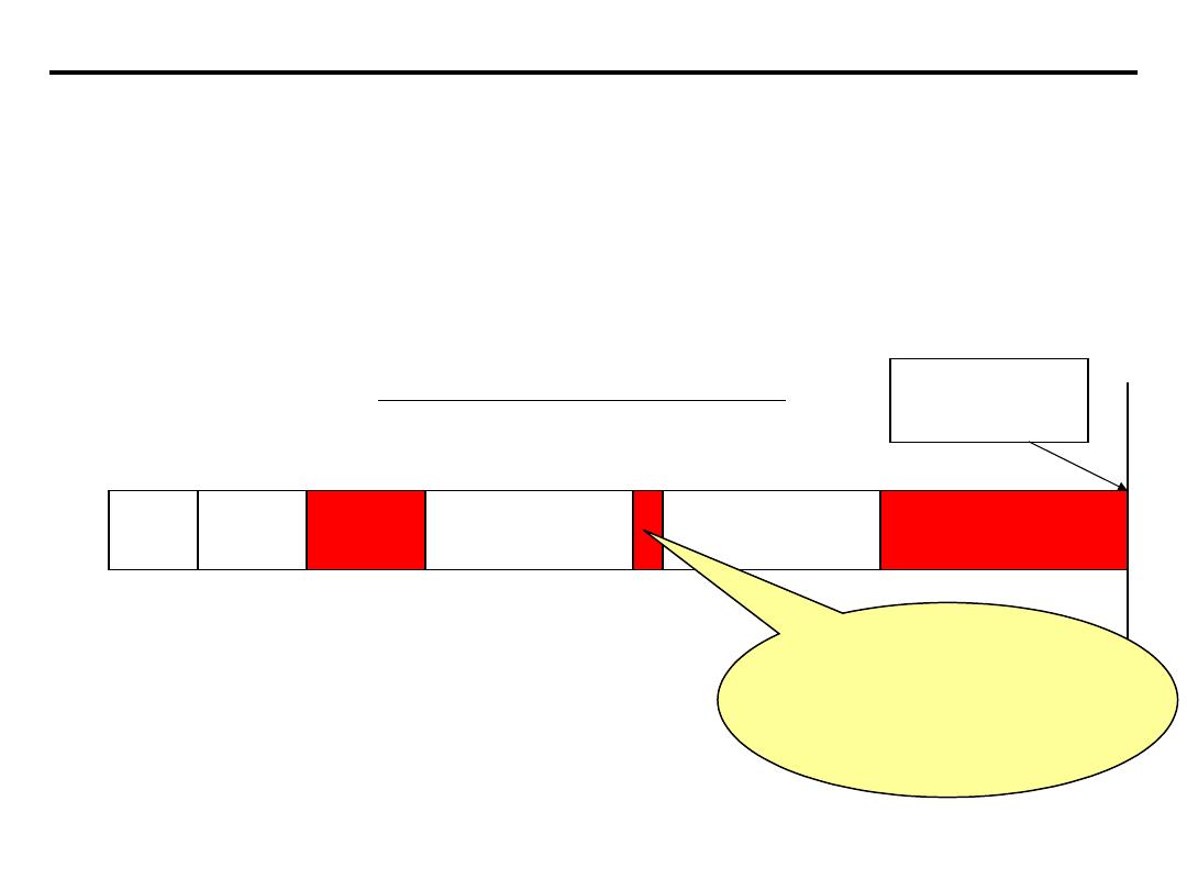
OS level energy management: Inter-task EDF
1) Static voltage scaling EDF
2) Cycle conserving RT-DVS
3) Look-Ahead RT-DVS
1. Static Voltage Scaling EDF: Motivation
wc1
wc2
wc3
wc4
Holes in the pre-run schedule imply
:
EDF Test
:
∑(
wc
i
/p
i
) < 1
at frequency = F
max
In other words, whenever
∑(wc
i
/p
i
) < 1 there are holes in the EDF
schedule
Next arrival
of T1
Pre-run schedule with holes
WC
i
= worst case computation time @ F
max
Processor typically idles
during holes.
Instead, the holes can be
exploited to slowdown
the processor to save
energy
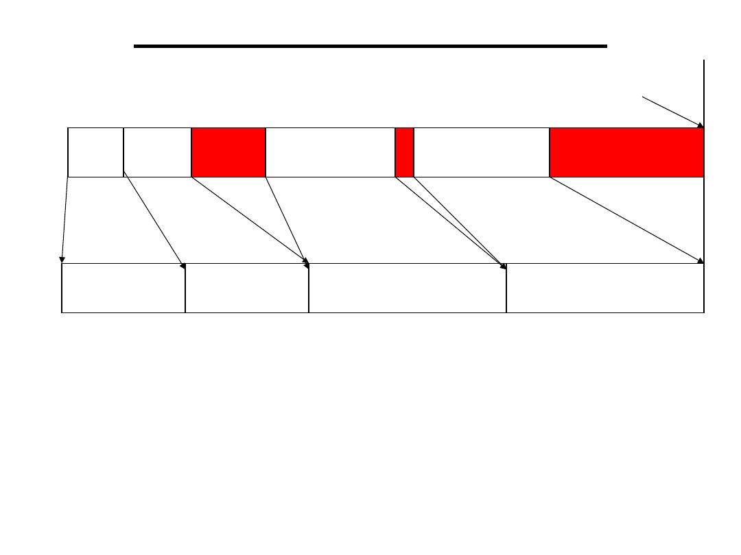
Static Voltage Scaling EDF
wc1
wc2
wc3
wc4
K*wc1
K *wc2
K * wc3
K * wc4
EDF Test
:
∑(
wc
i
/p
i
) < 1
at maximum frequency = F
max
Static-VS EDF Test
:
K* [∑(wc
i
/p
i
)] = 1
at frequency = F
max
/K
Next arrival
of T1
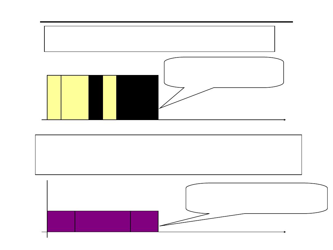
Static voltage scaling: Example
Task set: T1 = (1, 4) and T2 = (2, 8)
U = 1/4 + 2/8 = 0.5 (< 1) @ Fmax
Finding the right frequency scaling parameter (say, k)
U = (1*k)/4 + (2*k)/8 = 0.5*k = 1 @ (F
max
/k)
This gives, k = 2. Therefore, operating frequency = F
max
/2
0
1
3 4
5
8
F
re
qu
en
cy
F
m
Time
F
re
qu
en
cy
F
m
F
m
/ 2
Energy consumption
:
1
*
F^2 + 2*F^2 = 3F^2
Energy consumption
:
1
*(
F/2)^2 + 2*(F/2)^2 = (¾)F^2
0
2
6
8
Time
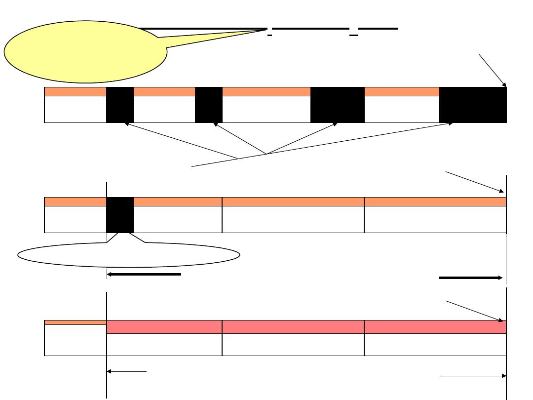
What if (C
i
< WC
i
)??
Actual
computation time
K*c1
K *c2
K * c3
K * c4
Next arrival
of T1
More holes left unexploited
K*c1
K *wc2
K * wc3
K * wc4
Next arrival of T1
Task T1 completes
Slow down all these tasks proportionally
Hole of size = (wc1 –
c1
)
K*c1
K’ *wc2
K’ * wc3
K’ * wc4
Next arrival of T1
CPU Cycles are conserved by slowing down the
remaining tasks

Real-time Languages
• Support for the management of time
– Language constructs for expressing timing constraint,
keeping track of resource utilization.
• Schedulability analysis
– Aid compile-time schedulability check.
• Reusable real-time software modules
– Object-oriented methodology.
• Support for distributed programming and fault-tolerance

Real-time Databases
Conventional database systems
• Disk-based.
• Use transaction logging and two-phase locking protocols to ensure
transaction atomicity and serializability.
• These characteristics preserve data integrity, but they also result in
relatively slow and unpredictable response times.
Real-time database system
, issues include:
– transaction scheduling to meet deadlines.
– explicit semantics for specifying timing and other constraints.
– checking the database system’s ability of meeting transaction deadlines
during application initialization.