
Uni
Electro
iversity of
omechani
Energy
f Technolo
cal Depar
Branch
ogy
tment
Advance Mathematics
Laplace Transformation
2 Class
nd
Lecture 6
Page 1 of 37

Definition
Suppose that f(t) is a piecewise continuous function. The Laplace transform of f(t) is
denoted
( )
{
}
f t
L
and defined as
( )
{
}
( )
0
st
f t
f t dt
¥ -
=
ò
e
L
(1)
There is an alternate notation for Laplace transforms. For the sake of convenience we will often
denote Laplace transforms as,
( )
{
}
( )
f t
F s
=
L
Example 1
If
0
c
¹
, evaluate the following integral.
0
ct
dt
¥
ò
e
Solution
Remember that you need to convert improper integrals to limits as follows,
0
0
lim
n
n
ct
ct
dt
dt
¥
®¥
=
ò
ò
e
e
Now, do the integral, then evaluate the limit.
0
0
0
lim
1
lim
1
1
lim
n
n
n
n
n
ct
ct
ct
cn
dt
dt
c
c
c
¥
®¥
®¥
®¥
=
æ
ö
=
ç
÷
è
ø
æ
ö
=
-
ç
÷
è
ø
ò
ò
e
e
e
e
Now, at this point, we’ve got to be careful. The value of c will affect our answer. We’ve already
assumed that c was non-zero, now we need to worry about the sign of c. If c is positive the
exponential will go to infinity. On the other hand, if c is negative the exponential will go to zero.
So, the integral is only convergent (i.e. the limit exists and is finite) provided c<0. In this case
we get,
0
1
provided
0
ct
dt
c
c
¥
= -
<
ò
e
(2)
Now that we remember how to do these, let’s compute some Laplace transforms. We’ll start off
with probably the simplest Laplace transform to compute.
Example 2
Compute
L{1}.
Solution
There’s not really a whole lot do here other than plug the function f(t) = 1 into (1)
{ }
0
1
st
dt
¥ -
=
ò
e
L
Now, at this point notice that this is nothing more than the integral in the previous example with
c
s
= -
. Therefore, all we need to do is reuse (2) with the appropriate substitution. Doing this
gives,
{ }
0
1
1
provided
0
st
dt
s
s
¥ -
=
= -
- <
-
ò
e
L
Or, with some simplification we have,
{ }
1
1
provided
0
s
s
=
>
L
Laplace Transformation
Dr.Eng Muhammad.A.R.yass
Page 2 of 37

Example 3
Compute
{ }
at
e
L
Solution
Plug the function into the definition of the transform and do a little simplification.
{ }
(
)
0
0
a s t
at
st at
dt
dt
¥
¥
-
-
=
=
ò
ò
e
e e
e
L
Once again, notice that we can use (2) provided
c a s
= -
. So let’s do this.
{ }
(
)
0
1
provided
0
1
provided
a s t
at
dt
a s
a s
s a
¥
-
=
= -
- <
-
=
>
ò
e
e
L
Example 4
Compute
L{sin(at)}.
Solution
Note that we’re going to leave it to you to check most of the integration here. Plug the function
into the definition. This time let’s also use the alternate notation.
( )
{
}
( )
( )
( )
0
0
sin
sin
lim
sin
st
n
st
n
at
F s
at dt
at dt
¥ -
-
®¥
=
=
=
ò
ò
e
e
L
Now, if we integrate by parts we will arrive at,
( )
( )
( )
0
0
1
lim
cos
cos
n
n
st
st
n
s
F s
at
at dt
a
a
-
-
®¥
æ
ö
æ
ö
=
-
-
ç
÷
ç
÷
ç
÷
è
ø
è
ø
ò
e
e
Now, evaluate the first term to simplify it a little and integrate by parts again on the integral.
Doing this arrives at,
( )
( )
(
)
( )
( )
0
0
1
1
lim
1
cos
sin
sin
n
n
sn
st
st
n
s
s
F s
an
at
at dt
a
a
a
a
-
-
-
®¥
æ
ö
æ
ö
æ
ö
ç
÷
=
-
-
+
ç
÷
ç
÷
ç
÷
ç
÷
è
ø
è
ø
è
ø
ò
e
e
e
Now, evaluate the second term, take the limit and simplify.
s-a
( )
( )
(
)
( )
( )
( )
( )
0
0
2
2
0
1
1
lim
1
cos
sin
sin
1
sin
1
sin
n
sn
sn
st
n
st
st
s
s
F s
an
an
at dt
a
a a
a
s s
at dt
a a a
s
at dt
a a
-
-
-
®¥
¥ -
¥ -
æ
ö
æ
ö
=
-
-
+
ç
÷
ç
÷
è
ø
è
ø
æ
ö
= - ç
÷
è
ø
= -
ò
ò
ò
e
e
e
e
e
Now, simply solve for F(s) to get,
( )
{
}
( )
2
2
sin
provided
0
a
at
F s
s
s
a
=
=
>
+
L
Dr.Eng Muhammad.A.R.yass
Page 3 of 37

Fact
Given f(t) and g(t) then,
( )
( )
{
}
( )
( )
af t
bg t
a F s
bG s
+
=
+
L
for any constants a and b.
1
Find the Laplace transforms of the given functions.
Example
(a)
( )
5
3
3
6
5
9
t
t
f t
t
-
=
+
+
-
e
e
( )
( )
3 1
4
1
1
3!
1
6
5
9
5
3
6
1
30 9
5
3
F s
s
s
s
s
s
s
s
s
+
=
+
+
-
- -
-
=
+
+
-
+
-
(b)
( )
( )
( )
( )
4cos 4
9sin 4
2cos 10
g t
t
t
t
=
-
+
( )
( )
( )
( )
2
2
2
2
2
2
2
2
2
4
4
9
2
4
4
10
4
36
2
16
16
100
s
s
G s
s
s
s
s
s
s
s
s
=
-
+
+
+
+
=
-
+
+
+
+
(c)
( )
( )
( )
3sinh 2
3sin 2
h t
t
t
=
+
( )
( )
( )
2
2
2
2
2
2
2
2
3
3
2
2
6
6
4
4
H s
s
s
s
s
=
+
-
+
=
+
-
+
(d)
( )
( )
( )
3
3
cos 6
cos 6
t
t
g t
t
t
=
+
-
e
e
( )
( ) (
) ( )
(
)
2
2
2
2
2
2
1
3
3
6
3
6
1
3
3
36
3
36
s
s
G s
s
s
s
s
s
s
s
s
-
=
+
-
-
+
-
+
-
=
+
-
-
+
-
+
Example 2
Find the transform of each of the following functions.
(a)
( )
( )
cosh 3
f t
t
t
=
( )
( )
{
}
( )
( )
( )
,
where
cosh 3
F s
tg t
G s
g t
t
¢
=
= -
=
L
So, we then have,
( )
( )
(
)
2
2
2
2
9
9
9
s
s
G s
G s
s
s
+
¢
=
= -
-
-
Using #30 we then have,
( )
(
)
2
2
2
9
9
s
F s
s
+
=
-
Dr.Eng Muhammad.A.R.yass
*
Multiply by t
Dr.Eng Muhammad.A.R.yass
Page 4 of 37

(b)
( )
( )
2
sin 2
h t
t
t
=
This part will also use
#30
in the table. In fact we could use #30 in one of two ways. We could
use it with
1
n
=
.
( )
( )
{
}
( )
( )
( )
,
where
sin 2
H s
tf t
F s
f t
t
t
¢
=
= -
=
L
Or we could use it with
2
n
=
.
( )
( )
{
}
( )
( )
( )
2
,
where
sin 2
H s
t f t
F s
f t
t
¢¢
=
=
=
L
Since it’s less work to do one derivative, let’s do it the first way. So using
#9
we have,
( )
(
)
( )
(
)
2
2
3
2
2
4
12
16
4
4
s
s
F s
F s
s
s
-
¢
=
= -
+
+
The transform is then,
( )
(
)
2
3
2
12
16
4
s
H s
s
-
=
+
(c)
( )
3
2
g t
t
=
This part can be done using either
#6
(with
2
n
=
) or
#32
(along with
#5
). We will use #32 so
we can see an example of this. In order to use #32 we’ll need to notice that
3
3
2
2
0
0
2
3
3
2
t
t
v dv
t
t
v dv
=
Þ
=
ò
ò
Now, using #5,
( )
( )
3
2
2
f t
t
F s
s
p
=
=
we get the following.
( )
5
3
2
2
3
1
3
2
4
2
G s
s
s
s
p
p
æ
öæ ö
=
=
ç
÷ç ÷
ç
÷è ø
è
ø
This is what we would have gotten had we used #6.
(d)
( ) ( )
3
2
10
f t
t
=
( )
3
2
g t
t
=
then
( )
( )
10
f t
g
t
=
Therefore, the transform is.
( )
5
2
3
2
5
2
1
10
10
1
3
10
4
10
3
10
4
s
F s
G
s
s
p
p
æ
ö
=
ç
÷
è
ø
æ
ö
ç
÷
ç
÷
=
ç
÷
æ
ö
ç
÷
ç
÷
ç
÷
è
ø
è
ø
=
(e)
( )
( )
f t
tg t
¢
=
This final part will again use
#30
from the table as well as
#35
.
( )
{
}
{ }
( ) ( )
{
}
( )
( )
(
)
( )
( )
0
0
d
tg t
g
ds
d
sG s
g
ds
G s
sG s
G s
sG s
¢
¢
= -
= -
-
¢
= -
+
-
¢
= -
-
L
L
Remember that g(0) is just a constant so when we differentiate it we will get zero!
For this part we’ll will use
#24
along with the answer from the previous part. To see this note
that if
Dr.Eng Muhammad.A.R.yass
Page 5 of 37
*
Dividing by t
Dr.Eng Muhammad.A.R.yass
Page 6 of 37
Laplace Transformation of periodic Function
Dr.Eng Muhammad.A.R.yass
Page 7 of 37
Dr.Eng Muhammad.A.R.yass
Page 8 of 37

Ch64-H8152.tex
23/6/2006
15: 16
Page 631
K
3. (a) 5e
3t
(b) 2e
−2t
(a)
5
s
− 3
(b)
2
s
+ 2
4. (a) 4 sin 3t (b) 3 cos 2t
(a)
12
s
2
+ 9
(b)
3s
s
2
+ 4
5. (a) 7 cosh 2x (b)
1
3
sinh 3t
(a)
7s
s
2
− 4
(b)
1
s
2
− 9
6. (a) 2 cos
2
t (b) 3 sin
2
2x
(a)
2(s
2
+ 2)
s(s
2
+ 4)
(b)
24
s(s
2
+ 16)
7. (a) cosh
2
t (b) 2 sinh
2
2θ
(a)
s
2
− 2
s(s
2
− 4)
(b)
16
s(s
2
− 16)
8. 4 sin(at
+ b), where a and b are constants
4
s
2
+ a
2
(a cos b
+ s sin b)
9. 3 cos(ωt
− α), where ω and α are constants
3
s
2
+ ω
2
(s cos α
+ ω sin α)
10. Show that
L
(cos
2
3t
− sin
2
3t)
=
s
s
2
+ 36
1. (a) 2t
− 3 (b) 5t
2
+ 4t − 3
(a)
2
s
2
−
3
s
(b)
10
s
3
+
4
s
2
−
3
s
2. (a)
t
3
24
− 3t + 2 (b)
t
5
15
− 2t
4
+
t
2
2
(a)
1
4s
4
−
3
s
2
+
2
s
(b)
8
s
6
−
48
s
5
+
1
s
3
laplace Home work
1. (a) 2te
2t
(b) t
2
e
(a)
2
(s
− 2)
2
(b)
2
(s
− 1)
3
2. (a) 4t
3
e
−2t
(b)
1
2
t
4
e
−3t
(a)
24
(s
+ 2)
4
(b)
12
(s
+ 3)
5
3. (a) e
t
cos t (b) 3e
2t
sin 2t
(a)
s
− 1
s
2
− 2s + 2
(b)
6
s
2
− 4s + 8
4. (a) 5e
−2t
cos 3t (b) 4e
−5t
sin t
(a)
5(s
+ 2)
s
2
+ 4s + 13
(b)
4
s
2
+ 10s + 26
5. (a) 2e
t
sin
2
t (b)
1
2
e
3t
cos
2
t
⎡
⎢
⎢
⎣
(a)
1
s
− 1
−
s
− 1
s
2
− 2s + 5
(b)
1
4
1
s
− 3
+
s
− 3
s
2
− 6s + 13
⎤
⎥
⎥
⎦
6. (a) e
t
sinh t (b) 3e
2t
cosh 4t
(a)
1
s(s
− 2)
(b)
3(s
− 2)
s
2
− 4s − 12
7. (a) 2e
−t
sinh 3t (b)
1
4
e
−3t
cosh 2t
(a)
6
s
2
+ 2s − 8
(b)
s
+ 3
4(s
2
+ 6s + 5)
8. (a) 2e
t
( cos 3t
− 3 sin 3t)
(b) 3e
−2t
( sinh 2t
− 2 cosh 2t)
(a)
2(s
− 10)
s
2
− 2s + 10
(b)
−6(s + 1)
s(s
+ 4)
1
1
1
1
1
1
1
1
Dr.Eng Muhammad.A.R.yass
Page 9 of 37

Inverse Laplace Transforms
( )
( )
{
}
1
f t
F s
-
=
L
As with Laplace transforms, we’ve got the following fact to help us take the inverse transform.
Fact
Given the two Laplace transforms F(s) and G(s) then
( )
( )
{
}
( )
{
}
( )
{
}
1
1
1
aF s
bG s
a
F s
b
G s
-
-
-
+
=
+
L
L
L
for any constants a and b.
Example 1
Find the inverse transform of each of the following.
(a)
( )
6
1
4
8
3
F s
s
s
s
= -
+
-
-
( )
( ) ( )
( )
8
3
8
3
1
1
1
6
4
8
3
6 1
4
6
4
t
t
t
t
F s
s s
s
f t
=
-
+
-
-
=
-
+
= -
+
e
e
e
e
(b)
( )
5
19
1
7
2 3
5
H s
s
s
s
=
-
+
+
-
.
( )
( )
(
)
( )
4!
4!
4 1
5
3
4 1
5
3
7
19
1
2
3
1
1 1
7 4!
19
2
3
4!
H s
s
s
s
s
s
s
+
+
=
-
+
- -
-
=
-
+
- -
-
.
( )
5
3
2
4
1
7
19
3
24
t
t
h t
t
-
=
-
+
e
e
(c)
( )
2
2
6
3
25
25
s
F s
s
s
=
+
+
+
( )
( )
( )
( )
( )
5
5
2
2
2
2
2
2
2
2
3
6
5
5
3
5
6
5
5
5
s
F s
s
s
s
s
s
=
+
+
+
=
+
+
+
gives,
( )
( )
( )
3
6 cos 5
sin 5
5
f t
t
t
=
+
(d)
( )
2
2
8
3
3
12
49
G s
s
s
=
+
+
-
Dr.Eng Muhammad.A.R.yass
Page 10 of 37
( )
( )( )
( )
( )
2
2
7
7
2
2
2
2
1
8
3
3
4
49
4 2
3
1
3
2
7
G s
s
s
s
s
=
+
+
-
=
+
+
-
( )
( )
( )
4
3
sin 2
sinh 7
3
7
g t
t
t
=
+
Example 2
Find the inverse transform of each of the following.
(a)
( )
2
6
5
7
s
F s
s
-
=
+
( )
( )
( )
( )
7
7
2
2
5
6
7
7
5
6 cos
7
sin
7
7
s
F s
s
s
f t
t
t
=
-
+
+
=
-
(b)
( )
2
1 3
8
21
s
F s
s
s
-
=
+
+
.
(
)
2
2
2
2
8
21
8
16 16 21
8
16 5
4
5
s
s
s
s
s
s
s
+
+
=
+
+
- +
=
+
+
+
= +
+
( )
(
)
2
1 3
4
5
s
F s
s
-
=
+
+
( )
(
)
(
)
(
)
(
)
(
)
2
2
2
1 3
4 4
4
5
1 3
4
12
4
5
3
4
13
4
5
s
F s
s
s
s
s
s
-
+ -
=
+
+
-
+ +
=
+
+
-
+
+
=
+
+
( )
( )
(
)
(
)
( )
( )
( )
5
5
2
2
4
4
13
4
3
4
5
4
5
13
3
cos
5
sin
5
5
t
t
s
F s
s
s
f t
t
t
-
-
+
= -
+
+
+
+
+
= -
+
e
e
(c)
( )
2
3
2
2
6
2
s
G s
s
s
-
=
-
-
( )
(
)
(
)
2
2
9
9
4
4
2
3
13
2
4
3
2
2
3
1
1
3
2
2
3
1
1
3
2
2
s
G s
s
s
s
s
s
s
s
-
=
- -
-
=
- + - -
-
=
-
-
Dr.Eng Muhammad.A.R.yass
Page 11 of 37

( )
(
)
(
)
(
)
(
)
(
)
(
)
(
)
( )
3
3
2
2
3
3
2
2
2
3
13
2
4
3
5
2
2
2
3
13
2
4
13
5
3
2
2
13
2
2
3
13
3
13
2
4
2
4
3
2
1
2
3
1
2
3
1
2
1
13
5
13
3
cosh
sinh
2
2
2
13
t
t
s
G s
s
s
s
s
s
s
g t
t
t
- + -
=
-
-
- +
=
-
-
æ
ö
-
ç
÷
=
+
ç
÷
-
-
-
-
è
ø
æ
ö
æ
ö
æ
ö
=
+
ç
÷
ç
÷
ç
÷
ç
÷
ç
÷
ç
÷
è
ø
è
ø
è
ø
e
e
(d)
( )
2
7
3
10
s
H s
s
s
+
=
- -
( ) ( )( )
7
2
5
s
H s
s
s
+
=
+
-
( )
2
5
A
B
H s
s
s
=
+
+
-
(
)(
)
(
)
(
)
(
)(
)
5
2
7
2
5
2
5
A s
B s
s
s
s
s
s
- +
+
+
=
+
-
+
-
(
)
(
)
7
5
2
s
A s
B s
+ =
- +
+
( )
( )
5
5
7
0
7
A
B
A
=
- +
Þ = -
picking s. We can B in the same way if we chos
( )
( )
12
12
0
7
7
A
B
B
=
+
Þ
=
t when it does it will usually simplify the work c
transform becomes,
( )
5
12
7
7
2
5
H s
s
s
-
=
+
+
-
( )
2
5
5
12
7
7
t
t
h t
-
= -
+
e
e
Factor in
denominator
Term in partial
fraction decomposition
ax b
+
A
ax b
+
(
)
k
ax b
+
(
)
(
)
1
2
2
k
k
A
A
A
ax b
ax b
ax b
+
+ +
+
+
+
L
2
ax
bx c
+
+
2
Ax B
ax
bx c
+
+
+
(
)
2
k
ax
bx c
+
+
(
)
(
)
1
1
2
2
2
2
2
2
k
k
k
A x B
A x B
A x B
ax
bx c
ax
bx c
ax
bx c
+
+
+
+
+ +
+
+
+
+
+
+
L
Dr.Eng Muhammad.A.R.yass
Dr.Eng Muhammad.A.R.yass
Page 12 of 37

Example 3
Find the inverse transform of each of the following.
(a)
( ) ( )( )( )
86
78
3
4 5
1
s
G s
s
s
s
-
=
+
-
-
( )
3
4 5
1
A
B
C
G s
s
s
s
=
+
+
+
-
-
(
)(
)
(
)(
)
(
)(
)
86
78
4 5
1
3 5
1
3
4
s
A s
s
B s
s
C s
s
-
=
-
- +
+
- +
+
-
As with the last example, we can easily get the constants by correctly picking values of s.
( )(
)
( )( )
3
336
7
16
3
1
304
16
19
5
5
5
5
5
4
266
7 19
2
s
A
A
s
C
C
s
B
B
= -
-
=
-
-
Þ
= -
æ
öæ
ö
=
-
=
-
Þ
=
ç
֍
÷
è
øè
ø
=
=
Þ
=
So, the partial fraction decomposition for this transform is,
( )
3
2
5
3
4 5
1
G s
s
s
s
= -
+
+
+
-
-
( )
( )
5
1
5
3
4
3
2
1
3
4
3
2
t
t
t
G s
s
s
s
g t
-
= -
+
+
+
-
-
= -
+
+
e
e
e
(b)
( )
(
)
(
)
2
2 5
6
11
s
F s
s
s
-
=
-
+
So, for the first time we’ve got a quadratic in the denominator. Here’s the decomposition for thi
part.
( )
2
6
11
A
Bs C
F s
s
s
+
=
+
-
+
Setting numerators equal gives,
(
)
(
)(
)
2
2 5
11
6
s
A s
Bs C s
-
=
+
+
+
-
(
)
(
)(
)
(
)
(
)
2
2
2
2
2 5
11
6
11
6
6
6
11
6
s
A s
Bs C s
As
A Bs
B Cs
C
A B s
B C s
A
C
-
=
+
+
+
-
=
+
+
-
+
-
=
+
+ -
+
+
-
2
1
0
:
0
28
28
67
:
6
5
,
,
47
47
47
: 11
6
2
s
A B
s
B C
A
B
C
s
A
C
ü
+ =
ï
-
+ = -
Þ
= -
=
= -
ý
ï
-
=
þ
( )
2
11
11
2
2
1
28
28
67
47
6
11
67
1
28
28
47
6
11
11
s
F s
s
s
s
s
s
s
-
æ
ö
=
-
+
ç
÷
-
+
è
ø
æ
ö
=
-
+
-
ç
÷
ç
÷
-
+
+
è
ø
( )
( )
( )
6
1
67
28
28cos 11
sin
11
47
11
t
f t
t
t
æ
ö
=
-
+
-
ç
÷
è
ø
e
Dr.Eng Muhammad.A.R.yass
Page 13 of 37

(c)
( )
(
)
3
2
25
4
5
G s
s s
s
=
+
+
( )
2
3
2
4
5
A
B
C
Ds E
G s
s
s
s
s
s
+
= +
+
+
+
+
Setting numerators equal and multiplying out gives.
(
)
(
) (
)
(
)
(
)
(
)
(
)
(
)
2
2
2
2
3
4
3
2
25
4
5
4
5
4
5
4
5
4
5
4
5
As s
s
Bs s
s
C s
s
Ds E s
A D s
A B E s
A
B C s
B
C s
C
=
+
+ +
+
+ +
+
+ +
+
=
+
+
+ +
+
+
+
+
+
+
3
2
1
0
:
0
: 4
0
11
11
24
,
4,
5,
,
: 5
4
0
5
5
5
:
5
4
0
:
5
25
s
A D
s
A B E
A
B
C
D
E
s
A
B C
s
B
C
s
C
+ =
ï
+ + =
ïï
Þ
=
= -
=
= -
= -
+
+ = ý
ï
+
= ï
ï
=
þ
( )
2
3
2
1 11 20 25
11
24
5
4
5
s
G s
s
s
s
s
s
+
æ
ö
=
-
+
-
ç
÷
+
+
è
ø
( )
(
)
(
)
(
)
(
)
(
)
2
3
2
2
2
3
2!
2!
2
2
2
3
1 11 20 25
11
24
5
4
5
11
2 2
24
1 11 20 25
5
2
1
11
2
25
1 11 20
2
5
2
1
2
1
s
G s
s
s
s
s
s
s
s
s
s
s
s
s
s
s
s
s
+
æ
ö
=
-
+
-
ç
÷
+
+
è
ø
æ
ö
+ - +
=
-
+
-
ç
÷
ç
÷
+
+
è
ø
æ
ö
+
=
-
+
-
-
ç
÷
ç
÷
+
+
+
+
è
ø
then.
( )
( )
( )
2
2
2
1
25
11 20
11
cos
2
sin
5
2
t
t
g t
t
t
t
t
-
-
æ
ö
=
-
+
-
-
ç
÷
e
e
Dr.Eng Muhammad.A.R.yass
Page 14 of 37
Step Functions
Before proceeding into solving differential equations we should take a look at one more function.
Without Laplace transforms it would be much more difficult to solve differential equations that
involve this function in g(t).
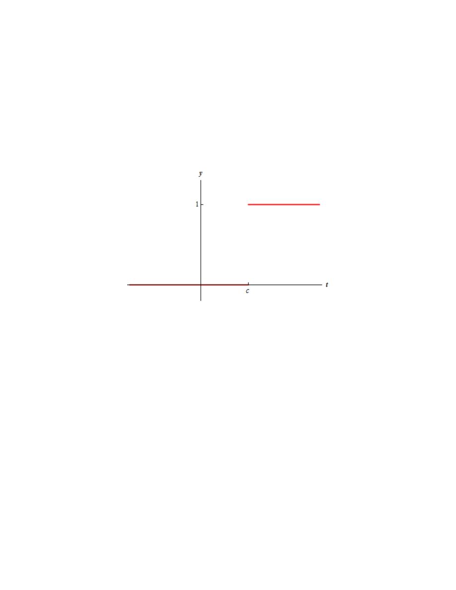
The function is the Heaviside function and is defined as,
( )
0 if
1 if
c
t c
u t
t c
<
ì
= í
³
î
Here is a graph of the Heaviside function.
Heaviside functions are often called step functions. Here is some alternate notation for Heaviside
functions.
( )
(
)
(
)
c
u t
u t c
H t c
=
-
=
-
Example 1
Write the following function (or switch) in terms of Heaviside functions.
( )
4
if
6
25
if 6
8
16
if 8
30
10
if
30
t
t
f t
t
t
-
<
ì
ï
£ <
ï
= í
£ <
ï
ï
³
î
Solution
There are three sudden shifts in this function and so (hopefully) it’s clear that we’re going to need
three Heaviside functions here, one for each shift in the function. Here’s the function in terms of
Heaviside functions.
( )
( )
( )
( )
6
8
30
4 29
9
6
f t
u t
u t
u
t
= - +
-
-
It’s fairly easy to verify this.
In the first interval, t < 6 all three Heaviside functions are off and the function has the value
( )
4
f t
= -
Notice that when we know that Heaviside functions are on or off we tend to not write them at all
as we did in this case.
In the next interval,
6
8
t
£ <
the first Heaviside function is now on while the remaining two are
still off. So, in this case the function has the value.
( )
4 29 25
f t
= - +
=
Dr.Eng Muhammad.A.R.yass
Page 15 of 37
In the third interval,
8
30
t
£ <
the first two Heaviside functions are one while the last remains
off. Here the function has the value.
( )
4 29 9 16
f t
= - +
- =
In the last interval,
30
t
³
all three Heaviside function are one and the function has the value.
( )
4 29 9 6 10
f t
= - +
- - =
So, the function has the correct value in all the intervals.
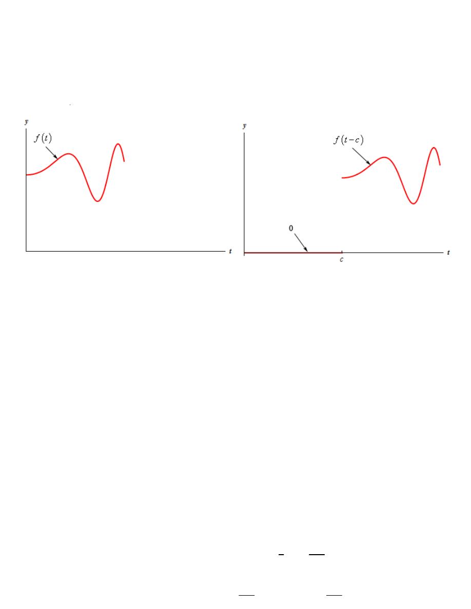
Using Heaviside functions this switch can be wrote as
( )
( ) (
)
c
g t
u t f t c
=
-
( ) (
)
{
}
( ) (
)
(
)
0
c
c
c
st
st
u t f t c
u t f t c dt
f t c dt
¥ -
¥ -
-
=
-
=
-
ò
ò
e
e
L
.
Now use the substitution u = t – c and the integral becomes,
( ) (
)
{
}
(
)
( )
( )
0
0
c
s u c
su
cs
u t f t c
f u du
f u du
¥ -
¥ -
-
+
-
=
=
ò
ò
e
e e
L
The second exponential has no u’s in it and so it can be factored out of the integral. Note as well
that in the substitution process the lower limit of integration went back to 0.
( ) (
)
{
}
( )
0
c
c s
su
u t f t c
f u du
¥
-
-
-
=
ò
e
e
L
Now, the integral left is nothing more than the integral that we would need to compute if we were
going to find the Laplace transform of f(t). Therefore, we get the following formula
( ) (
)
{
}
( )
c
c s
u t f t c
F s
-
-
= e
L
(2)
1
c
cs
F s
u t f t c
-
-
=
-
e
L
(3)
( )
{
}
( ) (
)
We can use (2) to get the Laplace transform of a Heaviside function by itself. To do this we will
consider the function in (2) to by f(t) = 1. Doing this gives us
( )
{
}
( )
{
}
{ }
1
1
1
c
c
c s
cs
c s
u t
u t
s
s
-
-
-
=
=
=
=
e
e
e
g
L
L
L
Putting all of this together leads to the following two formulas.
( )
{
}
( )
1
c
c
c s
c s
u t
u t
s
s
-
-
-
ì
ü
=
=
í
ý
î
þ
e
e
L
L
(4)
Dr.Eng Muhammad.A.R.yass
Page 16 of 37

Example 2
Find the Laplace transform of each of the following.
(a)
( )
( ) (
) ( )
(
)
( )
3
12 3
12
6
4
10
2
6
7
t
g t
u
t
t
u t
u t
-
=
+
-
- - e
are using the following function,
( )
(
) (
)
3
3
2
6
2
6
f t
t
f t
t
=
Þ
-
=
-
and this has been shifted by the correct amount.
The third term uses the following function,
( )
(
)
( )
3
4
3
12 3
7
4
7
7
t
t
t
f t
f t
-
-
-
-
= -
Þ
-
= -
= -
e
e
e
which has also been shifted by the correct amount.
With these functions identified we can now take the transform of the function.
( )
( )
12
6
4
3 1
12
6
4
3 1
2 3!
10
7
1
3
10
12
7
1
3
s
s
s
s
s
s
G s
s
s
s
s
s
s
s
s
-
-
-
+
-
-
-
+
æ
ö
=
+
-
-
ç
÷
+
è
ø
æ
ö
=
+
-
-
ç
÷
+
è
ø
e
e
e
e
e
e
(b)
( )
( )
( ) ( )
2
3
5
cos
f t
t u t
t u t
= -
+
. Here they are.
( )
(
) ( )
(
) ( )
2
3
5
3 3
cos
5 5
f t
t
u t
t
u t
= - - +
+
- +
( )
(
)
(
)
(
)
cos
5
5
cos
5 5
g t
t
g t
t
=
+
Þ
-
=
- +
This will make our life a little easier so we’ll do it this way.
Now, breaking up the first term and leaving the second term along gives us,
( )
(
)
(
)
(
)
( )
(
) ( )
2
3
5
3
6
3
9
cos
5 5
f t
t
t
u t
t
u t
= -
-
+
- +
+
- +
Okay, so it looks like the two functions that have been shifted here are
( )
( )
(
)
2
6
9
cos
5
g t
t
t
g t
t
= + +
=
+
Taking the transform then gives,
( )
( )
( )
3
5
3
2
2
cos 5
sin 5
2
6
9
1
s
s
s
F s
s
s
s
s
-
-
-
æ
ö
æ
ö
= -
+
+
+ ç
÷
ç
÷
+
è
ø
è
ø
e
e
(c)
( )
4
4
if
5
1
3sin
if
5
10 2
t
t
h t
t
t
t
ì
<
ï
= í
æ
ö
+
-
³
ç
÷
ï
è
ø
î
This one isn’t as bad as it might look on the surface. The first thing that we need to do is writ
in terms of Heaviside functi ons.
( )
( )
( )
(
)
4
5
4
5
1
3
sin
10 2
1
3
sin
5
10
t
h t
t
u t
t
u t
t
æ
ö
= +
-
ç
÷
è
ø
æ
ö
= +
-
ç
÷
è
ø
All we need to do now is to take the transform.
( )
( )
( )
5
1
10
2
5
2
1
10
5
3
10
5
2
1
1
00
3
4!
24
s
s
H s
s
s
s
s
-
-
=
+
+
=
+
+
e
e
Dr.Eng Muhammad.A.R.yass
Page 17 of 37

(d)
( )
(
)
2
if
6
8
6
if
6
t
t
f t
t
t
<
ìï
= í
- + -
³
ïî
Again, the first thing that we need to do is write the function in terms of Heaviside functions.
( )
(
)
(
)
( )
2
6
8
6
f t
t
t
t
u t
= + - - + -
Here is the corrected function.
( )
(
) (
)
(
)
( )
(
)
(
)
(
)
( )
(
) (
)
(
)
( )
2
6
2
6
2
6
8
6 6
6
8
6
6
6
14
6
6
f t
t
t
t
u t
t
t
t
u t
t
t
t
u t
= + - - - + + -
= + - - - - + -
= + - - - + -
So, in the second term it looks like we are shifting
( )
2
14
g t
t
t
= - -
The transform is then,
( )
6
2
3
2
1
2
1
14
s
F s
s
s
s
s
-
æ
ö
=
+
-
-
ç
÷
è
ø
e
Example 3
Find the inverse Laplace transform of each of the following.
(a)
( ) (
)(
)
4
3
2
2
s
s
H s
s
s
-
=
+
-
e
( )
(
)(
)
( )
4
4
3
2
2
s
s
s
H s
F s
s
s
-
-
=
=
+
-
e
e
( )
3
2
2
A
B
F s
s
s
=
+
+
-
Setting numerators equal gives,
(
)
(
)
2
3
2
s
A s
B s
=
- +
+
We’ll find the constants here by selecting values of s. Doing this gives,
1
2
2 8
4
2
2
8
1
3
3
3
4
s
B
B
s
A
A
=
=
Þ
=
= -
- = -
Þ
=
So, the partial fraction decomposition becomes,
( )
(
)
1
1
4
4
2
3
3
2
F s
s
s
=
+
+
-
Notice that we factored a 3 out of the denominator in order to actually do the inverse transform.
The inverse transform of this is then,
( )
2
3
2
1
1
12
4
t
t
f t
-
=
+
e
e
Now, let’s go back and do the actual problem. The original transform was,
( )
( )
4s
H s
F s
-
= e
( )
( ) (
)
4
4
h t
u t f t
=
-
where, f(t) is,
( )
2
3
2
1
1
12
4
t
t
f t
-
=
+
e
e
Dr.Eng Muhammad.A.R.yass
Page 18 of 37

(b)
( )
(
)
(
)
6
11
2
5
3
2
9
s
s
G s
s
s
-
-
-
=
+
+
e
e
( )
(
)
(
)
(
)
(
)
6
11
2
2
5
3
2
9
2
9
s
s
G s
s
s
s
s
-
-
=
-
+
+
+
+
e
e
( )
(
)
(
)
(
)
(
)
6
11
2
2
1
1
5
3
2
9
2
9
s
s
G s
s
s
s
s
-
-
=
-
+
+
+
+
e
e
( )
(
)
(
)
( )
6
11
6
11
2
1
5
3
5
3
2
9
s
s
s
s
G s
F s
s
s
-
-
-
-
=
-
=
-
+
+
e
e
e
e
(
)
(
)
and now we will just partial fraction F(s).
Here is the partial fraction decomposition.
( )
2
2
9
A
Bs C
F s
s
s
+
=
+
+
+
Setting numerators equal and combining gives us,
(
)
(
)(
)
(
)
(
)
2
2
1
9
2
2
9
2
A s
s
Bs C
A B s
B C s
A
C
=
+ + +
+
=
+
+
+
+
+
Setting coefficient equal and solving gives,
2
1
0
:
0
1
1
2
: 2
0
,
,
13
13
13
: 9
2
1
s
A B
s
B C
A
B
C
s
A
C
ü
+ =
ï
+ =
Þ
=
= -
=
ý
ï
+
= þ
Substituting back into the transform gives and fixing up the numerators as needed gives,
( )
2
3
3
2
2
1
1
2
13
2
9
2
1
1
13
2
9
9
s
F s
s
s
s
s
s
s
- +
æ
ö
=
+
ç
÷
+
+
è
ø
æ
ö
=
-
+
ç
÷
+
+
+
è
ø
little simpler. Taking the inverse transform then gives,
( )
( )
( )
2
1
2
cos 3
sin 3
13
3
t
f t
t
t
-
æ
ö
=
-
+
ç
÷
è
ø
e
At this point we can go back and start thinking about the original problem.
( )
(
)
( )
( )
( )
6
11
6
11
5
3
5
3
s
s
s
s
G s
F s
F s
F s
-
-
-
-
=
-
=
-
e
e
e
e
We’ll also need to distribute the F(s) through as well in order to get the correct
Recall that in order to use (3) to take the inverse transform you must have a si
times a single transform. This means that we must multiply the F(s) through t
can now take the inverse transform,
( )
( ) (
)
( ) (
)
6
11
5
6
3
11
g t
u t f t
u t f t
=
- -
-
where,
( )
( )
( )
2
1
2
cos 3
sin 3
13
3
t
f t
t
t
-
æ
ö
=
-
+
ç
÷
è
ø
e
(c)
( ) ( )( )
4
1
2
s
s
F s
s
s
-
+
=
-
+
e
Dr.Eng Muhammad.A.R.yass
Page 19 of 37

In this case, unlike the previous part, we will need to break up the transform since one term has a
constant in it and the other has an s. Note as well that we don’t consider the exponential in this,
only its coefficient. Breaking up the transform gives,
( ) ( )( ) ( )( ) ( )
( )
4
1
1
2
1
2
s
s
s
F s
G s
H s
s
s
s
s
-
-
=
+
=
+
-
+
-
+
e
e
We will need to partial fraction both of these terms up. We’ll start with G(s).
( )
1
2
A
B
G s
s
s
=
+
-
+
Setting numerators equal gives,
(
)
(
)
4
2
1
s
A s
B s
=
+
+
-
Now, pick values of s to find the constants.
8
2
8
3
3
4
1
4 3
3
s
B
B
s
A
A
= -
- = -
Þ
=
=
=
Þ
=
So G(s) and its inverse transform is,
( )
( )
8
4
3
3
2
1
2
4
8
3
3
t
t
G s
s
s
g t
-
=
+
-
+
=
+
e
e
Now, repeat the process for H(s).
( )
1
2
A
B
H s
s
s
=
+
-
+
Setting numerators equal gives,
(
)
(
)
1
2
1
A s
B s
=
+ +
-
Now, pick values of s to find the constants.
1
2
1
3
3
1
1
1 3
3
s
B
B
s
A
A
= -
= -
Þ
= -
=
=
Þ
=
So H(s) and its inverse transform is,
( )
( )
1
1
3
3
2
1
2
1
1
3
3
t
t
H s
s
s
h t
-
=
-
-
+
=
-
e
e
Putting all of this together gives the following,
( )
( )
( )
( )
( )
( ) (
)
1
1
s
F s
G s
H s
f t
g t
u t h t
-
=
+
=
+
-
e
where,
( )
( )
2
2
4
8
1
1
and
3
3
3
3
t
t
t
t
g t
h t
-
-
=
+
=
-
e
e
e
e
Dr.Eng Muhammad.A.R.yass
Page 20 of 37

(d)
( )
(
)
20
3
7
2
3
8
2
6
3
s
s
s
s
s
G s
s s
-
-
-
+
-
+
=
+
e
e
e
This one looks messier than it actually is. Let’s first rearrange the numerator a little.
( )
(
) (
)
(
)
3
20
7
2
3 2
8
6
3
s
s
s
s
G s
s s
-
-
-
-
+
+
=
+
e
e
e
In this form it looks like we can break this up into two pieces that will require partial fractions.
When we break these up we should always try and break things up into as few pieces as possible
for the partial fractioning. Doing this can save you a great deal of unnecessary work. Breaking
up the transform as suggested above gives,
( )
(
)
(
)
(
)
(
)
(
)
( )
(
)
( )
3
20
7
2
3
20
7
1
1
3 2
8
6
3
3
3 2
8
6
s
s
s
s
s
s
G s
s s
s s
F s
H s
-
-
-
-
-
-
= -
+
+
+
+
= -
+
+
e
e
e
e
e
e
Note that we canceled an s in F(s). You should always simplify as much a possible before doing
the partial fractions.
Let’s partial fraction up F(s) first.
( )
3
A
B
F s
s
s
=
+
+
Setting numerators equal gives,
(
)
1
3
A s
Bs
=
+ +
Now, pick values of s to find the constants.
1
3
1
3
3
1
0
1 3
3
s
B
B
s
A
A
= -
= -
Þ
= -
=
=
Þ
=
So F(s) and its inverse transform is,
( )
( )
1
1
3
3
3
3
1 1
3 3
t
F s
s s
f t
-
= -
+
= - e
Now partial fraction H(s).
( )
2
3
A
B
C
H s
s
s
s
=
+
+
+
Setting numerators equal gives,
(
)
(
)
2
1
3
3
As s
B s
Cs
=
+ +
+ +
Dr.Eng Muhammad.A.R.yass
Page 21 of 37

Pick values of s to find the constants.
1
3
1 9
9
1
0
1 3
3
13
1
1
1 4
4
4
9
9
s
C
C
s
B
B
s
A
B C
A
A
= -
=
Þ
=
=
=
Þ
=
=
=
+
+ =
+
Þ
= -
So H(s) and its inverse transform is,
( )
( )
1
1
1
9
3
9
2
3
3
1 1
1
9 3
9
t
H s
s s
s
h t
t
-
= - +
+
+
= - +
+ e
Now, let’s go back to the original problem, remembering to multiply the transform through the
parenthesis.
( )
( )
( )
( )
( )
3
20
7
3
2
8
6
s
s
s
G s
F s
F s
H s
H s
-
-
-
=
-
+
+
e
e
e
Taking the inverse transform gives,
( )
( )
( ) (
)
( ) (
)
( ) (
)
3
20
7
3
2
3
8
20
6
7
g t
f t
u t f t
u
t h t
u t h t
=
-
- +
-
+
-
Dr.Eng Muhammad.A.R.yass
Dr.Eng Muhammad.A.R.yass
Page 22 of 37

Ch66-H8152.tex
23/6/2006
15: 16
Page 640
1. (a)
7
s
(b)
2
s
− 5
[(a) 7 (b) 2e
5t
]
2. (a)
3
2s
+ 1
(b)
2s
s
2
+ 4
(a)
3
2
e
−
1
2
t
(b) 2 cos 2t
3. (a)
1
s
2
+ 25
(b)
4
s
2
+ 9
(a)
1
5
sin 5t
(b)
4
3
sin 3t
4. (a)
5s
2s
2
+ 18
(b)
6
s
2
(a)
5
2
cos 3t
(b) 6t
5. (a)
5
s
3
(b)
8
s
4
(a)
5
2
t
2
(b)
4
3
t
3
6. (a)
3s
1
2
s
2
− 8
(b)
7
s
2
− 16
(a) 6 cosh 4t
(b)
7
4
sinh 4t
7. (a)
15
3s
2
− 27
(b)
4
(s
− 1)
3
(a)
5
3
sinh 3t
(b) 2 e
t
t
2
8. (a)
1
(s
+ 2)
4
(b)
3
(s
− 3)
5
(a)
1
6
e
−2t
t
3
(b)
1
8
e
3t
t
4
9. (a)
s
+ 1
s
2
+ 2s + 10
(b)
3
s
2
+ 6s + 13
(a) e
−t
cos 3t
(b)
3
2
e
−3t
sin 2t
10. (a)
2(s
− 3)
s
2
− 6s + 13
(b)
7
s
2
− 8s + 12
(a) 2e
3t
cos 2t
(b)
7
2
e
4t
sinh 2t
11. (a)
2s
+ 5
s
2
+ 4s − 5
(b)
3s
+ 2
s
2
− 8s + 25
⎡
⎢
⎣
(a) 2e
−2t
cosh 3t
+
1
3
e
−2t
sinh 3t
(b) 3e
4t
cos 3t
+
14
3
e
4t
sin 3t
⎤
⎥
⎦
Inverse Laplace Transformation
Dr.Eng Muhammad.A.R.yass
Page 23 of 37

Solving IVP’s with Laplace Transforms
Fact
Suppose that f, f’, f”,…f
(n-1)
are all continuous functions and f
(n)
is a piecewise continuous
function. Then,
( )
{ }
( )
( )
( )
(
)
( )
(
)
( )
2
1
1
2
0
0
0
0
n
n
n
n
n
n
f
s F s
s
f
s
f
sf
f
-
-
-
-
¢
=
-
-
- -
-
L
L
Since we are going to be dealing with second order differential equations it will be convenient to
have the Laplace transform of the first two derivatives.
{ }
( ) ( )
{ }
( )
( )
( )
2
0
0
0
y
sY s
y
y
s Y s
sy
y
¢ =
-
¢¢
¢
=
-
-
L
L
Example 1
Solve the following IVP.
( )
( )
10
9
5 ,
0
1
0
2
y
y
y
t
y
y
¢¢
¢
¢
-
+
=
= -
=
Solution
The first step in using Laplace transforms to solve an IVP is to take the transform of every term in
the differential equation.
{ }
{ }
{ }
{ }
10
9
5
y
y
y
t
¢¢
¢
-
+
=
L
L
L
L
Using the appropriate formulas from our
table of Laplace transforms
gives us the following.
( )
( )
( )
( ) ( )
(
)
( )
2
2
5
0
0
10
0
9
s Y s
sy
y
sY s
y
Y s
s
¢
-
-
-
-
+
=
Plug in the initial conditions and collect all the terms that have a Y(s) in them.
(
)
( )
2
2
5
10
9
12
s
s
Y s
s
s
-
+
+ -
=
Solve
for Y (s).
( )
(
)(
) (
)(
)
2
5
12
9
1
9
1
s
Y s
s s
s
s
s
-
=
+
-
-
-
-
Combining the two terms gives,
( )
(
)(
)
2
3
2
5 12
9
1
s
s
Y s
s s
s
+
-
=
-
-
The partial fraction decomposition for this transform is,
( )
2
9
1
A
B
C
D
Y s
s
s
s
s
= +
+
+
-
-
Setting numerators equal gives,
(
)(
)
(
)(
)
(
)
(
)
2
3
2
2
5 12
9
1
9
1
1
9
s
s
As s
s
B s
s
Cs s
Ds s
+
- =
-
- +
-
- +
- +
-
Picking appropriate values of s and solving for the constants gives,
5
0
5 9
9
1
16
8
2
31
9
248 648
81
4345
50
2
45
14
81
81
s
B
B
s
D
D
s
C
C
s
A
A
=
=
Þ
=
=
= -
Þ
= -
=
=
Þ
=
=
= -
+
Þ
=
Plugging in the constants gives,
( )
50
5
31
81
9
81
2
2
9
1
Y s
s
s
s
s
=
+
+
-
-
-
Finally taking the inverse transform gives us the solution to the IVP.
( )
9
50 5
31
2
81 9
81
t
t
y t
t
=
+
+
-
e
e
Dr.Eng Muhammad.A.R.yass
Page 24 of 37

Example 2
Solve the following IVP.
( )
( )
2
2
3
2
,
0
0
0
2
t
y
y
y t
y
y
-
¢¢
¢
¢
+
-
=
=
= -
e
Solution
As with the first example, let’s first take the Laplace transform of all the terms in the differential
equation. We’ll the plug in the initial conditions to get,
( )
( )
( )
(
)
( ) ( )
(
)
( )
(
)
(
)
( )
(
)
2
2
2
2
1
2
0
0
3
0
2
2
1
2
3
2
4
2
s Y s
sy
y
sY s
y
Y s
s
s
s
Y s
s
¢
-
-
+
-
-
=
+
+
-
+ =
+
Now solve for Y(s).
( )
(
)(
) (
)(
)
3
1
4
2
1
2
2
1
2
Y s
s
s
s
s
=
-
-
+
-
+
Now, as we did in the last example we’ll go ahead and combine the two terms together as we will
have to partial fraction up the first denominator anyway, so we may as well make the numerator a
little more complex and just do a single partial fraction. This will give,
( )
(
)
(
)(
)
(
)(
)
2
3
2
3
1 4
2
2
1
2
4
16
15
2
1
2
s
Y s
s
s
s
s
s
s
-
+
=
-
+
-
-
-
=
-
+
( )
(
) (
)
2
3
2
1
2
2
2
A
B
C
D
Y s
s
s
s
s
=
+
+
+
-
+
+
+
Setting numerator equal gives,
(
)
(
)(
)
(
)(
)
(
)
(
)
(
)
(
)
3
2
2
3
2
4
16
15
2
2
1
2
2
1
2
2
1
2
6
7
2
12
4
3
2
8
4
2
s
s
A s
B s
s
C
s
s
D s
A
B s
A
B
C s
A
B
C
D s
A
B
C D
-
-
-
=
+
+
-
+
+
-
+
+
-
=
+
+
+
+
+
+
+
+
+
-
-
-
In this case it’s probably easier to just set coefficients equal and solve the resulting system of
equation rather than pick values of s. So, here is the system and its solution.
3
2
1
0
:
2
0
192
96
:
6
7
2
4
125
125
2
1
:12
4
3
2
16
25
5
: 8
4
2
15
s
A
B
A
B
s
A
B
C
s
A
B
C
D
C
D
s
A
B
C D
ü
+
=
= -
=
ï
+
+
= - ï
Þ
ý
+
+
+
= - ï
= -
= -
ï
-
-
- = - þ
We will get a common denominator of 125 on all these coefficients and factor that out when we
go to plug them back into the transform. Doing this gives,
( )
(
)
(
) (
)
2!
2!
2
3
1
2
25
1
192
96
10
125 2
2
2
2
Y s
s
s
s
s
æ
ö
-
=
+
-
-
ç
÷
ç
÷
-
+
+
+
è
ø
Taking the inverse transform then gives,
( )
2
2
2
2
2
1
25
96
96
10
125
2
t
t
t
t
y t
t
t
-
-
-
æ
ö
=
-
+
-
-
ç
÷
è
ø
e
e
e
e
Dr.Eng Muhammad.A.R.yass
Page 25 of 37

Example 3
Solve the following IVP.
( )
( )
( )
6
15
2sin 3 ,
0
1
0
4
y
y
y
t
y
y
¢¢
¢
¢
-
+
=
= -
= -
Solution
Take the Laplace transform of everything and plug in the initial conditions.
( )
( )
( )
( ) ( )
(
)
( )
(
)
( )
2
2
2
2
3
0
0
6
0
15
2
9
6
6
15
2
9
s Y s
sy
y
sY s
y
Y s
s
s
s
Y s
s
s
¢
-
-
-
-
+
=
+
-
+
+ - =
+
Now solve for Y(s) and combine into a single term as we did in the previous two examples.
( )
(
)(
)
3
2
2
2
2
9
24
9
6
15
s
s
s
Y s
s
s
s
- +
-
+
=
+
-
+
Now, do the partial fractions on this. First let’s get the partial fraction decomposition.
( )
2
2
9
6
15
As B
Cs D
Y s
s
s
s
+
+
=
+
+
-
+
Now, setting numerators equal gives,
(
)
(
)
(
)
(
)
(
)
(
)
(
)
3
2
2
2
3
2
2
9
24
6
15
9
6
15
6
9
15
9
s
s
s
As B s
s
Cs D s
A C s
A B D s
A
B
C s
B
D
- +
-
+
=
+
-
+
+
+
+
=
+
+ -
+ +
+
-
+
+
+
Setting coefficients equal and solving for the constants gives,
3
2
1
0
:
1
1
1
:
6
2
10
10
11
5
:15
6
9
9
10
2
:
15
9
24
s
A C
A
B
s
A B D
s
A
B
C
C
D
s
B
D
ü
+ = -
=
=
ï
-
+ + = ï
Þ
ý
-
+
= - ï
= -
=
ï
+
=
þ
Now, plug these into the decomposition, complete the square on the denominator of the second
term and then fix up the numerators for the inverse transform process.
( )
(
)
(
)
2
2
2
2
1
1
11
25
10
9
6
15
11
3 3
25
1
1
10
9
3
6
s
s
Y s
s
s
s
s
s
s
s
+
-
+
æ
ö
=
+
ç
÷
+
-
+
è
ø
æ
ö
-
- + +
+
=
+
ç
÷
ç
÷
+
-
+
è
ø
(
)
(
)
(
)
6
3
6
3
2
2
2
2
8
11
3
1
1
10
9
9
3
6
3
6
s
s
s
s
s
s
æ
ö
-
=
ç
+
-
-
÷
ç
÷
+
+
-
+
-
+
è
ø
Finally, take the inverse transform.
( )
( )
( )
( )
( )
3
3
1
1
8
cos 3
sin 3
11 cos
6
sin
6
10
3
6
t
t
y t
t
t
t
t
æ
ö
=
+
-
-
ç
÷
è
ø
e
e
Dr.Eng Muhammad.A.R.yass
Page 26 of 37

Ch67-H8152.tex
23/6/2006
15: 16
Page 648
1. A first order differential equation involving
current i in a series R
−L circuit is given by:
di
dt
+ 5i =
E
2
and i
= 0 at time t = 0.
Use Laplace transforms to solve for i
when (a) E
= 20 (b) E = 40 e
−3t
and (c)
E
= 50 sin 5t.
⎡
⎢
⎢
⎣
(a) i
= 2(1 − e
−5t
)
(b) i
= 10( e
−3t
− e
−5t
)
(c) i
=
5
2
( e
−5t
− cos 5t + sin 5t)
⎤
⎥
⎥
⎦
In Problems 2 to 9, use Laplace transforms to
solve the given differential equations.
2. 9
d
2
y
dt
2
− 24
dy
dt
+ 16y = 0, given y(0) = 3
and y
(0)
= 3.
y
= (3 − t) e
4
3
t
3.
d
2
x
dt
2
+ 100x = 0, given x(0) = 2 and
x
(0)
= 0.
[x
= 2 cos 10t]
4.
d
2
i
dt
2
+ 1000
di
dt
+ 250000i = 0, given
i(0)
= 0 and i
(0)
= 100. [i = 100t e
−500t
]
5.
d
2
x
dt
2
+ 6
dx
dt
+ 8x = 0, given x(0) = 4 and
x
(0)
= 8.
[x
= 4(3e
−2t
− 2e
−4t
)]
6.
d
2
y
dx
2
− 2
dy
dx
+ y = 3 e
4x
, given y(0)
= −
2
3
and y
(0)
= 4
1
3
y
= (4x − 1) e
x
+
1
3
e
4x
7.
d
2
y
dx
2
+ 16y = 10 cos 4x, given y(0) = 3 and
y
(0)
= 4.
y
= 3 cos 4x + sin 4x +
5
4
x sin 4x
8.
d
2
y
dx
2
+
dy
dx
− 2y = 3 cos 3x − 11 sin 3x,
given y(0)
= 0 and y
(0)
= 6
[y
= e
x
− e
−2x
+ sin 3x]
9.
d
2
y
dx
2
− 2
dy
dx
+ 2y = 3 e
x
cos 2x, given
y(0)
= 2 and y
(0)
= 5
y
= 3e
x
( cos x
+ sin x) − e
x
cos 2x
Home Work
Dr.Eng Muhammad.A.R.yass
Page 27 of 37
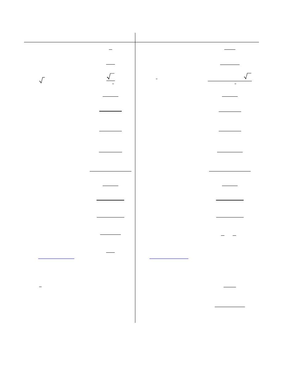
Table of Laplace Transforms
( )
( )
{
}
1
f t
F s
-
=
L
( )
( )
{
}
F s
f t
=
L
( )
( )
{
}
1
f t
F s
-
=
L
( )
( )
{
}
F s
f t
=
L
1.
1
1
s
2.
at
e
1
s a
-
3.
,
1, 2,3,
n
t
n
=
K
1
!
n
n
s
+
4.
p
t
, p > -1
(
)
1
1
p
p
s
+
G
+
5.
t
3
2
2s
p
6.
1
2
,
1, 2,3,
n
t
n
-
=
K
(
)
1
2
1 3 5
2
1
2
n
n
n
s
p
+
× ×
-
L
7.
( )
sin at
2
2
a
s
a
+
8.
( )
cos at
2
2
s
s
a
+
9.
( )
sin
t
at
(
)
2
2
2
2as
s
a
+
10.
( )
cos
t
at
(
)
2
2
2
2
2
s
a
s
a
-
+
11.
( )
( )
sin
cos
at
at
at
-
(
)
3
2
2
2
2a
s
a
+
12.
( )
( )
sin
cos
at
at
at
+
(
)
2
2
2
2
2as
s
a
+
13.
( )
( )
cos
sin
at
at
at
-
(
)
(
)
2
2
2
2
2
s s
a
s
a
-
+
14.
( )
( )
cos
sin
at
at
at
+
(
)
(
)
2
2
2
2
2
3
s s
a
s
a
+
+
15.
(
)
sin at b
+
( )
( )
2
2
sin
cos
s
b
a
b
s
a
+
+
16.
(
)
cos at b
+
( )
( )
2
2
cos
sin
s
b
a
b
s
a
-
+
17.
( )
sinh at
2
2
a
s
a
-
18.
( )
cosh at
2
2
s
s
a
-
19.
( )
sin
at
bt
e
(
)
2
2
b
s a
b
-
+
20.
( )
cos
at
bt
e
(
)
2
2
s a
s a
b
-
-
+
21.
( )
sinh
at
bt
e
(
)
2
2
b
s a
b
-
-
22.
( )
cosh
at
bt
e
(
)
2
2
s a
s a
b
-
-
-
23.
,
1, 2,3,
n at
t
n
=
e
K
(
)
1
!
n
n
s a
+
-
24.
( )
f ct
1
s
F
c
c
æ ö
ç ÷
è ø
25.
( )
(
)
c
u t
u t c
=
-
Heaviside Function
cs
s
-
e
26.
(
)
t c
d -
Dirac Delta Function
cs
-
e
27.
( ) (
)
c
u t f t c
-
( )
cs
F s
-
e
28.
( ) ( )
c
u t g t
(
)
{
}
cs
g t c
-
+
e
L
29.
( )
ct
f t
e
(
)
F s c
-
30.
( )
,
1, 2,3,
n
t f t
n
=
K
( )
( )
( )
1
n
n
F
s
-
31.
( )
1
f t
t
( )
s
F u du
¥
ò
32.
( )
0
t
f v dv
ò
( )
F s
s
33.
(
) ( )
0
t
f t
g
d
t
t t
-
ò
( ) ( )
F s G s
34.
(
)
( )
f t T
f t
+
=
( )
0
1
T
st
sT
f t dt
-
-
-
ò
e
e
35.
( )
f t
¢
( )
( )
0
sF s
f
-
36.
( )
f t
¢¢
( )
( )
( )
2
0
0
s F s
sf
f ¢
-
-
37.
( )
( )
n
f
t
( )
( )
( )
(
)
( )
(
)
( )
2
1
1
2
0
0
0
0
n
n
n
n
n
s F s
s
f
s
f
sf
f
-
-
-
-
¢
-
-
-
-
L
Dr.Eng Muhammad.A.R.yass
Page 28 of 37

The solution of simultaneous differential equations using
Laplace transforms
It is sometimes necessary to solve simultaneous dif-ferential equations. An example occurs when two
electrical circuits are coupled magnetically where the equations relating the two currents i
1
and i
2
are
typically:
L
1
di
1
dt
+ M
di
2
dt
+ R
1
i
1
= E
1
L
2
di
2
dt
+ M
di
1
dt
+ R
2
i
2
= 0
where L represents inductance, R resistance, M mutual inductance and E
1
the p.d. applied to one
of the circuits.
(i) Take the Laplace transform of both sides of each simultaneous equation by applying the formu-
lae for the Laplace transforms of derivatives (i.e.
(ii) Put in the initial conditions, i.e. x(0), y(0), x
(0), y
(0).
(iii) Solve the simultaneous equations for
L
{y} and
L
{x} by the normal algebraic method.
(iv) Determine y and x by using, where necessary, partial fractions, and taking the inverse of each term.
Procedure
d y
dt
+ x = 1
dx
dt
− y + 4e
t
= 0
given that at t
= 0, x = 0 and y = 0.
Using the above procedure:
(i)
L
dy
dt
+
L
{x} =
L
{1}
(1)
L
dx
dt
−
L
{y} + 4
L
{e
t
} = 0
(2)
Equation (1) becomes:
[s
L
{y} − y(0)] +
L
{x} =
1
s
(1
)
from equation (3), page 634 and Table 64.1,
Example(1):- solve the following pair of simultaneous differential equation
Equation (2) becomes:
[s
L
{x} − x(0)] −
L
{y} = −
4
s
− 1
(2
)
(ii) x(0)
= 0 and y(0) = 0 hence
Equation (1
) becomes:
Dr Muhammad
A R Yass
Page 29 of 37

s
L
{y} +
L
{x} =
1
s
(1
)
and equation (2
) becomes:
s
L
{x} −
L
{y} = −
4
s
− 1
or
−
L
{y} + s
L
{x} = −
4
s
− 1
(2
)
(iii) 1
× equation (1
) and s
× equation (2
) gives:
s
L
{y} +
L
{x} =
1
s
(3)
−s
L
{y} + s
2
L
{x} = −
4s
s
− 1
(4)
Adding equations (3) and (4) gives:
(s
2
+ 1)
L
{x} =
1
s
−
4s
s
− 1
=
(s
− 1) − s(4s)
s(s
− 1)
=
−4s
2
+ s − 1
s(s
− 1)
from which,
L
{x} =
−4s
2
+ s − 1
s(s
− 1)(s
2
+ 1)
(5)
Using partial fractions
−4s
2
+ s − 1
s(s
− 1)(s
2
+ 1)
≡
A
s
+
B
(s
− 1)
+
Cs
+ D
(s
2
+ 1) =
A(s
− 1)(s
2
+ 1) + Bs(s
2
+ 1)
+ (Cs + D)s(s − 1)
s(s
− 1)(s
2
+ 1)
Hence
−4s
2
+ s − 1 = A(s − 1)(s
2
+ 1) + Bs(s
2
+ 1) + (Cs + D)s(s − 1)
When s
= 0, −1 = −A hence A = 1 When s = 1, −4 = 2B
hence B
= −2
Equating s
3
coefficients:
0
= A + B + C hence C = 1 (since A = 1 and B = −2)
Equating s
2
coefficients:
−4 = −A + D − C hence D = −2 (since A = 1 and C = 1)
Thus
L
{x} =
−4s
2
+ s − 1
s(s
− 1)(s
2
+ 1)
=
1
s
−
2
(s
− 1)
+
s
− 2
(s
2
+ 1)
(iv) Hence
x
=
L
−1
1
s
−
2
(s
− 1)
+
s
− 2
(s
2
+ 1)
=
L
−1
1
s
−
2
(s
− 1)
+
s
(s
2
+ 1)
−
2
(s
2
+ 1)
i.e.
x
= 1 − 2e
t
+ cos t − 2 sin t,
From the second equation given in the question,
Dr Muhammad
A R Yass
Page 30 of 37

dx
dt
− y + 4 e
t
= 0
from which,
y
=
dx
dt
+ 4 e
t
=
d
dt
(1
− 2 e
t
+ cos t − 2 sin t) + 4 e
t
= −2 e
t
− sin t − 2 cos t + 4 e
t
i.e. y
= 2e
t
− sin t − 2 cos t
[Alternatively, to determine y, return to equations (1
) and (2
)]
3
dx
dt
− 5
dy
dt
+ 2x = 6
2
dy
dt
−
dx
dt
− y = −1
given that at t
= 0, x = 8 and y = 3.
Using the above procedure:
(i) 3
L
dx
dt
− 5
L
dy
dt
+ 2
L
{x} =
L
{6}
(1)
2
L
dy
dt
−
L
dx
dt
−
L
{y} =
L
{−1}
(2)
Example(2):- solve the following pair of simultaneous differential equation
Equation (1) becomes:
3[s
L
{x} − x(0)] − 5[s
L
{y} − y(0)] + 2
L
{x} =
6
s
3s
L
{x} − 3x(0) − 5s
L
{y} + 5y(0) + 2
L
{x} =
6
s
.
(3s
+ 2)
L
{x} − 3x(0) − 5s
L
{y}+ 5y(0) =
6
s
(1
)
Equation (2) becomes:
2[s
L
{y} − y(0)] − [s
L
{x} − x(0)] −
L
{y} = −
1
s
2s
L
{y} − 2y(0) − s
L
{x}+ x(0) −
L
{y} = −
1
s
(2s
− 1)
L
{y} − 2y(0) − s
L
{x} + x(0) = −
1
s
(2
)
(ii)
x(0)
= 8 and y(0) = 3, hence equation (1
) becomes
(3s
+ 2)
L
{x} − 3(8) − 5s
L
{y}+ 5(3) =
6
s
(1
)
and equation (2
) becomes
(2s
− 1)
L
{y} − 2(3) − s
L
{x} + 8 = −
1
s
(2
)
i.e.
(3s
+ 2)
L
{x} − 5s
L
{y} =
6
s
+ 9
(1
)
(3s
+ 2)
L
{x} − 5s
L
{y} =
6
s
+ 9
(1
)
− s
L
{x} + (2s − 1)
L
{y} = −
1
s
− 2
(2
)
⎫
⎪
⎪
⎪
⎪
⎪
⎪
⎪
⎬
⎪
⎪
⎪
⎪
⎪
⎪
⎪
⎭
(A)
(iii)
s
× equation (1
) and (3s
+2) × equation (2
)
Dr Muhammad
A R Yass
Page 31 of 37

Ch68-H8152.tex
23/6/2006
15: 16
Page 652
gives:
s(3s
+ 2)
L
{x} − 5s
2
L
{y} = s
6
s
+ 9
(3)
−s(3s + 2)
L
{x} + (3s + 2)(2s − 1)
L
{y} = (3s + 2)
−
1
s
− 2
(4)
i.e.
s(3s
+ 2)
L
{x} − 5s
2
L
{y} = 6 + 9s (3
)
−s(3s + 2)
L
{x} + (6s
2
+ s − 2)
L
{y} = −6s −
2
s
− 7
(4
)
Adding equations (3
) and (4
) gives:
(s
2
+ s − 2)
L
{y} = −1 + 3s −
2
s
=
−s + 3s
2
− 2
s
from which,
L
{y} =
3s
2
− s − 2
s(s
2
+ s − 2)
Using partial fractions
3s
2
− s − 2
s(s
2
+ s − 2)
≡
A
s
+
B
(s
+ 2)
+
C
(s
− 1)
=
A(s
+ 2)(s − 1) + Bs(s − 1) + Cs(s + 2)
s(s
+ 2)(s − 1)
3s
2
− s − 2 = A(s + 2)(s − 1) + Bs(s − 1) + Cs(s + 2) When s = 0, −2 = −2A, hence A = 1
When
s
= 1, 0 = 3C, hence C = 0
When
s
= −2, 12 = 6B, hence B = 2
Thus
L
{y} =
3s
2
− s − 2
s(s
2
+ s − 2)
=
1
s
+
2
(s
+ 2)
(iv) Hence
y
=
L
−1
1
s
+
2
s
+ 2
= 1 + 2e
−2t
Returning to equations (A) to determine
L
{x} and hence x:
(2s
− 1) × equation (1
) and 5s
× (2
) gives:
(2s
− 1)(3s + 2)
L
{x} − 5s(2s − 1)
L
{y} = (2s − 1)
6
s
+ 9
(5)
and
−s(5s)
L
{x} + 5s(2s − 1)
L
{y} = 5s
−
1
s
− 2
(6)
(6s
2
+ s − 2)
L
{x} − 5s(2s − 1)
L
{y} = 12 + 18s −
6
s
− 9
(5
)
and
−5s
2
L
{x} + 5s(2s − 1)
L
{y} = −5 − 10s
(6
)
Adding equations (5
) and (6
) gives:
(s
2
+ s − 2)
L
{x} = −2 + 8s −
6
s
=
−2s + 8s
2
− 6
s
Dr Muhammad
A R Yass
Page 32 of 37

Ch68-H8152.tex
23/6/2006
15: 16
Page 653
K
from which,
L
{x} =
8s
2
− 2s − 6
s(s
2
+ s − 2) =
8s
2
− 2s − 6
s(s
+ 2)(s − 1)
Using partial fractions
8s
2
− 2s − 6
s(s
+ 2)(s − 1)
≡
A
s
+
B
(s
+ 2)
+
C
(s
− 1) =
A(s
+ 2)(s − 1) + Bs(s − 1) + Cs(s + 2)
s(s
+ 2)(s − 1)
8s
2
− 2s − 6 = A(s + 2)(s − 1) + Bs(s − 1) + Cs(s + 2)
When s
= 0, −6 = −2A
,
hence A
= 3 When s = 1, 0 = 3C, hence C = 0 When s = −2, 30 = 6B, hence B = 5
Thus
L
{x} =
8s
2
− 2s − 6
s(s
+ 2)(s − 1)
=
3
s
+
5
(s
+ 2)
Hence
x
=
L
−1
3
s
+
5
s
+ 2
= 3 + 5e
−2t
Therefore the solutions of the given simultaneous differential equations are
y
= 1 + 2e
−2t
and
x
= 3 + 5e
−2t
(These solutions may be checked by substituting the expressions for x and y into the original equations.)
d
2
x
dt
2
− x = y
d
2
y
dt
2
+ y = −x
given that at t
= 0, x = 2, y = −1,
dx
dt
= 0
and
dy
dt
= 0.
Using the procedure:
(i) [s
2
L
{x} − sx(0) − x
(0)]
−
L
{x} =
L
{y}
(1)
[s
2
L
{y} − sy(0) − y
(0)]
+
L
{y} = −
L
{x} (2)
(ii) x(0)
= 2, y(0) = −1, x
(0)
= 0 and y
(0)
= 0
hence
s
2
L
{x} − 2s −
L
{x} =
L
{y}
(1
)
s
2
L
{y} + s +
L
{y} = −
L
{x}
(2
)
(iii) Rearranging gives:
(s
2
− 1)
L
{x} −
L
{y} = 2s
(3)
L
{x} + (s
2
+ 1)
L
{y} = −s
(4)
Equation (3)
× (s
2
+ 1) and equation (4) × 1 gives:
(s
2
+ 1)(s
2
− 1)
L
{x} − (s
2
+ 1)
L
{y}= (s
2
+ 1)2s
(5)
L
{x} + (s
2
+ 1)
L
{y} = −s
(6)
Example(3):- solve the following pair of simultaneous differential equation
Adding equations (5) and (6) gives:
Dr Muhammad
A R Yass
Page 33 of 37

[(s
2
+ 1)(s
2
− 1) + 1]
L
{x} = (s
2
+ 1)2s − s
i.e.
s
4
L
{x} = 2s
3
+ s = s(2s
2
+ 1)
from which,
L
{x} =
s(2s
2
+ 1)
s
4
=
2s
2
+ 1
s
3
=
2s
2
s
3
+
1
s
3
=
2
s
+
1
s
3
(iv) Hence
x
=
L
−1
2
s
+
1
s
3
i.e.
x
= 2 +
1
2
t
2
Returning to equations (3) and (4) to deter-mine y:
1
× equation (3) and (s
2
− 1) × equation (4)
gives:
(s
2
− 1)
L
{x} −
L
{y} = 2s
(7)
(s
2
− 1)
L
{x} + (s
2
− 1)(s
2
+ 1)
L
{y} = −s(s
2
− 1)
(8)
Equation (7)
− equation (8) gives:
[
−1 − (s
2
− 1)(s
2
+ 1)]
L
{y} = 2s + s(s
2
− 1)
i.e.
−s
4
L
{y} = s
3
+ s
and
L
{y} =
s
3
+ s
−s
4
= −
1
s
−
1
s
3
from which,
y
=
L
−1
−
1
s
−
1
s
3
i.e.
y
= −1 −
1
2
t
2
Dr Muhammad
A R Yass
Page 34 of 37

Solve the following pairs of simultaneous dif- ferential equations:
1.
2
dx
dt
+
dy
dt
= 5 e
t
dy
dt
− 3
dx
dt
= 5
given that when t
= 0, x = 0 and y = 0
[x
= e
t
− t − 1 and y = 2t − 3 + 3e
t
]
2.
2
dy
dt
− y + x +
dx
dt
− 5 sin t = 0
3
dy
dt
+ x − y + 2
dx
dt
− e
t
= 0
given that at t
= 0, x = 0 and y = 0
x
= 5 cos t + 5 sin t − e
2t
− e
t
− 3 and
y
= e
2t
+ 2e
t
− 3 − 5 sin t
3.
d
2
x
dt
2
+ 2x = y
Further Problem
answer
answer
d
2
y
dt
2
+ 2y = x
given that at t
= 0, x = 4, y = 2,
dx
dt
= 0
and
dy
dt
= 0
x
= 3 cos t + cos (
√
3 t) and
y
= 3 cos t − cos (
√
3 t)
answer
Dr Muhammad
A R Yass
Page 35 of 37

Home Work
1. Find the Laplace transforms of the following functions:
(a) 2t
3
− 4t + 5 (b) 3e
−2t
− 4 sin 2t
(c) 3 cosh 2t
(d) 2t
4
e
−3t
(e) 5e
2t
cos 3t
(f) 2e
3t
sinh 4t
2. Find the inverse Laplace transforms of the fol- lowing functions:
(a)
5
2s
+ 1
(b)
12
s
5
(c)
4s
s
2
+ 9
(d)
5
s
2
− 9
(e)
3
(s
+ 2)
4
(f)
s
− 4
s
2
− 8s − 20
(g)
8
s
2
− 4s + 3
3. Use partial fractions to determine the following:
(a)
L
−1
5s
− 1
s
2
− s − 2
(b)
L
−1
2s
2
+ 11s − 9
s(s
− 1)(s + 3)
(c)
L
−1
13
− s
2
s(s
2
+ 4s + 13)
4. In a galvanometer the deflection θ satisfies the differential equation:
d
2
θ
dt
2
+ 2
dθ
dt
+ θ = 4 Use Laplace transforms to solve the equation for
θ
given that when t
= 0, θ = 0 and
dθ
dt
= 0
5. Solve the following pair of simultaneous differ- ential equations:
3
dx
dt
= 3x + 2y
2
dy
dt
+ 3x = 6y
given that when t
= 0, x = 1 and y = 3
Dr Muhammad
A R Yass
Page 36 of 37

Table Notes
1. This list is not inclusive and only contains some of the more commonly used Laplace
transforms and formulas.
2. Recall the definition of hyperbolic functions.
( )
( )
cosh
sinh
2
2
t
t
t
t
t
t
-
-
+
-
=
=
e
e
e
e
3. Be careful when using “normal” trig function vs. hyperbolic functions. The only
difference in the formulas is the “+ a
2
” for the “normal” trig functions becomes a “- a
2
”
for the hyperbolic functions!
4. Formula #4 uses the Gamma function which is defined as
( )
1
0
x t
t
x dx
¥ -
-
G
=
ò
e
If n is a positive integer then,
(
)
1
!
n
n
G + =
The Gamma function is an extension of the normal factorial function. Here are a couple
of quick facts for the Gamma function
(
)
( )
(
)(
) (
)
(
)
( )
1
1
2
1
1
2
p
p
p
p n
p p
p
p n
p
p
G
+ = G
G
+
+
+
+ - =
G
æ ö
G
=
ç ÷
è ø
L
Dr.Eng Muhammad.A.R.yass
Page 37 of 37