
2
nd
A
d
Clas
Adva
s
Uni
Electro
Lin
anc
iversity of
omechani
Energy
ne I
ed
f Technolo
cal Depar
Branch
Inte
Ma
ogy
tment
egra
athe
al
ema
atic
3
st
Le
cs
cture

Dr.Eng Muhammad.A.R.yass
Dr.Eng Muhammad.A.R.yass
Advance Mathematic
Line Integral
2 Class Electromechanical Engineer
nd
Dr.Eng.Muhammad.A.R.Yass
by
Page 2 of 21
Line Integral's
<<2012-2013>>

Dr.Eng Muhammad.A.R.yass
Dr.Eng Muhammad.A.R.yass
Multiple Integral
Green's Theorm
Stoke's Theorm
Page 3 of 21
Line Integral's
<<2013-2014>>
Dr.Eng Muhammad.A.R.yass
The line integral of
( )
,
f x y
along C is denoted by,
( )
,
C
f x y ds
ò
-
2
2
where
dx
dy
ds
dt
dt
dt
æ
ö
æ
ö
=
+
ç
÷
ç
÷
è
ø
è
ø
( )
( ) ( )
(
)
2
2
,
,
C
b
a
dx
dy
f x y ds
f h t
g t
dt
dt
dt
æ
ö
æ
ö
=
+
ç
÷
ç
÷
è
ø
è
ø
ó
ô
õ
ò
If we use the vector form of the parameterization we can simplify the notation up somewhat by
noticin that
Line Integral (with Respect To arc Length)
( )
2
2
dx
dy
r t
dt
dt
æ
ö
æ
ö
¢
+
=
ç
÷
ç
÷
è
ø
è
ø
r
where
( )
r t
¢r
is the
magnitude
or norm of
( )
r t
¢r
. Using this notation the line integral becomes
,
( )
( ) ( )
(
)
( )
,
,
C
b
a
f x y ds
f h t
g t
r t dt
¢
=
ò
ò
r
.
Example 1
Evaluate
4
C
xy ds
ò
where C is the right half of the circle,
2
2
16
x
y
+
=
rotated in the
counter clockwise direction.
Solution
4 cos
4 sin
x
t
y
t
=
=
right half of the circl
e
.
2
2
t
p
p
- £ £
and
4 sin
4 cos
dx
dy
t
t
dt
dt
= -
=
so r = 4 as we know that x=rcost and y=r sint so
for
2
2
16 sin
16 cos
4
ds
t
t dt
dt
=
+
=
The line integral is then,
(
) ( )
2
4
4
2
2
4
2
2
5
2
4 cos
4 sin
4
4096
cos sin
4096
sin
5
8192
5
C
xy ds
t
t
dt
t
t dt
t
p
p
p
p
p
p
-
-
-
=
=
=
=
ò
ò
ò
Page 4 of 21
Line Integral's
<<2013-2014>>
Dr.Eng Muhammad.A.R.yass
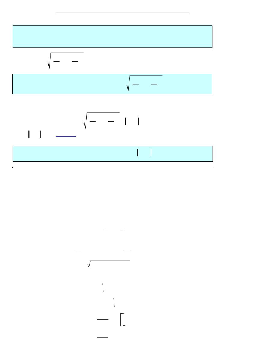
Example 2
Evaluate
3
4
C
x ds
ò
where C is the curve shown below.
Solution
So, first we need to parameterize each of the curves.
1
3
2
3
:
,
1,
2
0
:
,
1,
0
1
:
1,
,
0
2
C
x
t y
t
C
x
t y
t
t
C
x
y
t
t
=
= -
- £ £
=
= -
£ £
=
=
£ £
Now let’s do the line integral over each of these curves.
( ) ( )
1
0
0
0
2
2
3
3
3
4
2
2
2
4
4
1
0
4
16
C
x ds
t
dt
t dt
t
-
-
-
=
+
=
=
= -
ò
ò
ò
( )
( )
(
)
2
1
2
2
3
3
2
0
1
3
4
0
1
3
3
4
2
2
0
4
4
1
3
4
1 9
1 2
2
1 9
10
1
2.268
9 3
27
C
x ds
t
t
dt
t
t dt
t
=
+
=
+
æ
ö
æ ö
=
+
=
- =
ç
÷
ç ÷
è ø
è
ø
ó
ô
õ
ò
ò
( ) ( ) ( )
3
2
2
3
2
2
3
0
0
4
4 1
0
1
4
8
C
x ds
dt
dt
=
+
=
=
ò
ò
ò
Finally, the line integral that we were asked to compute is,
1
2
3
3
3
3
3
4
4
4
4
16 2.268 8
5.732
C
C
C
C
x ds
x ds
x ds
x ds
=
+
+
= - +
+
= -
ò
ò
ò
ò
Page 5 of 21
Line Integral's
<<2013-2014>>
Dr.Eng Muhammad.A.R.yass
Example 3
Evaluate
3
4
C
x ds
ò
were C is the line segment from
(
)
2, 1
- -
to
( )
1, 2
.
Solution
From the parameterization formulas at the start of this section we know that the line segment start
at
(
)
2, 1
- -
and ending at
( )
1, 2
is given by,
( ) (
)
1
2, 1
1, 2
2 3 , 1 3
r t
t
t
t
t
= -
- - +
= - +
- +
r
for
0
1
t
£ £
. This means that the individual parametric equations are,
2 3
1 3
x
t
y
t
= - +
= - +
Using this path the line integral is,
(
)
( )
(
)
1
3
3
0
1
4
1
12
0
4
4
2 3
9 9
12 2
2 3
5
12 2
4
15 2
21.213
C
x ds
t
dt
t
=
- +
+
=
- +
æ
ö
=
-
ç
÷
è
ø
= -
= -
ò
ò
Example 4
Evaluate
3
4
C
x ds
ò
were C is the line segment from
( )
1, 2
to
(
)
2, 1
- -
.
Solution
This one isn’t much different, work wise, from the previous example. Here is the
parameterization of the curve.
( ) (
)
1
1, 2
2, 1
1 3 , 2 3
r t
t
t
t
t
= -
+ - -
= -
-
r
for
0
1
t
£ £
. Remember that we are switch the direction of the curve and this will also change
the parameterization so we can make sure that we start/end at the proper point.
Here is the line integral.
(
)
( )
(
)
1
3
3
0
1
4
1
12
0
4
4 1 3
9 9
12 2
2 3
5
12 2
4
15 2
21 213
C
x ds
t
dt
t
=
-
+
=
- +
æ
ö
=
-
ç
÷
è
ø
= -
= -
ò
ò
We then have the following fact about line integrals with respect to arc length.
Page 6 of 21
Line Integral's
<<2013-2014>>
Dr.Eng Muhammad.A.R.yass
Fact
( )
( )
,
,
C
C
f x y ds
f x y ds
-
=
ò
ò
So, for a line integral with respect to arc length we can change the direction of the curve and not
change the value of the integral. This is a useful fact to remember as some line integrals will be
easier in one direction than the other.
Example 5
Evaluate
C
x ds
ò
for each of the following curves.
(a)
2
1
:
,
1
1
C
y
x
x
=
- £ £
(b)
2
C
: The line segment from
(
)
1,1
-
to
( )
1,1
.
(c)
3
C
: The line segment from
( )
1,1
to
(
)
1,1
-
.
Solution
(a)
2
1
:
,
1
1
C
y
x
x
=
- £ £
Here is a parameterization for this curve.
2
1
:
,
,
1
1
C
x
t y
t
t
=
=
- £ £
for
0
1
t
£ £
.
Here is the line integral.
(
)
1
1
3
1
2
2
2
1
1
1
1 4
1 4
0
12
C
x ds
t
t dt
t
-
-
=
+
=
+
=
ò
ò
(b)
2
C
: The line segment from
(
)
1,1
-
to
( )
1,1
.
( ) (
)
2
:
1
1,1
1,1
2
1,1
C
r t
t
t
t
= -
-
+
=
-
r
.
,
2
:
,
1,
1
1
C
x
t y
t
=
=
- £ £
Page 7 of 21
Line Integral's
<<2013-2014>>
Dr.Eng Muhammad.A.R.yass
This will be a much easier parameterization to use so we will use this. Here is the line integral
for this curve.
2
1
1
2
1
1
1
1 0
0
2
C
x ds
t
dt
t
-
-
=
+
=
=
ò
ò
(c)
3
C
: The line segment from
( )
1,1
to
(
)
1,1
-
.
since we know that
3
2
C
C
= -
. The fact tells us that this line integral should be the same
as the second part (i.e. zero). However, let’s verify that,
Here is the parameterization for this curve.
( ) (
)
3
:
1
1,1
1,1
1 2 ,1
C
r t
t
t
t
= -
+ -
= -
r
for
0
1
t
£ £
.
Here is the line integral for this curve.
(
)
(
)
3
1
1
2
0
0
1 2
4 0
2
0
C
x ds
t
dt
t
t
=
-
+
=
-
=
ò
ò
Sure enough we got the same answer as the second part.
Let’s suppose that the three-dimensional curve C is given by the parameterization,
( )
( )
( )
,
x
x t
y
y t
z
z t
a
t
b
=
=
=
£ £
then the line integral is given by,
(
)
( ) ( ) ( )
(
)
2
2
2
, ,
,
,
C
b
a
dx
dy
dz
f x y z ds
f x t
y t
z t
dt
dt
dt
dt
æ
ö
æ
ö
æ
ö
=
+
+
ç
÷
ç
÷
ç
÷
è
ø
è
ø
è
ø
ó
ô
õ
ò
Note that often when dealing with three-dimensional space the parameterization will be given as a
vector function.
( )
( ) ( ) ( )
,
,
r t
x t
y t
z t
=
r
Notice that we changed up the notation for the parameterization a little. Since we rarely use the
function names we simply kept the x, y, and z and added on the
( )
t
part to denote that they may
be functions of the parameter.
Also notice that, as with two-dimensional curves, we have,
( )
2
2
2
dx
dy
dz
r t
dt
dt
dt
æ
ö
æ
ö
æ
ö
¢
+
+
=
ç
÷
ç
÷
ç
÷
è
ø
è
ø
è
ø
r
and the line integral can again be written as,
(
)
( ) ( ) ( )
(
)
( )
, ,
,
,
C
b
a
f x y z ds
f x t
y t
z t
r t dt
¢
=
ò
ò
r
So, outside of the addition of a third parametric equation line integrals in three-dimensional space
work the same as those in two-dimensional space. Let’s work a quick example.
Page 8 of 21
Line Integral's
<<2013-2014>>
Dr.Eng Muhammad.A.R.yass
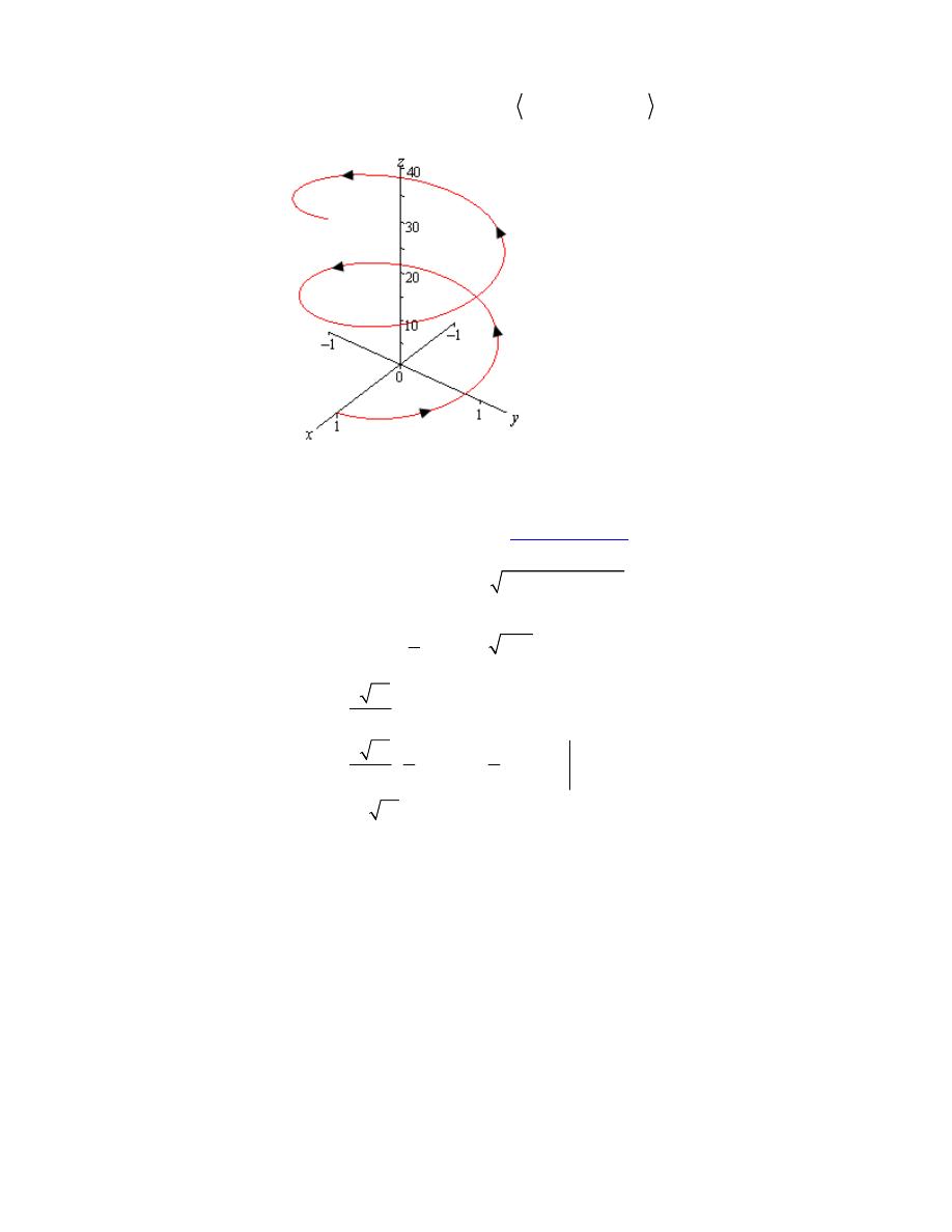
Example 6
Evaluate
C
xyz ds
ò
where C is the helix given by,
( )
( )
( )
cos
, sin
, 3
r t
t
t
t
=
r
,
0
4
t
p
£ £
.
Solution
Note that we first saw the vector equation for a helix back in the
Vector Functions
section. Her
is a quick sketch of the helix.
( ) ( )
( )
( )
( )
( )
4
2
2
0
4
0
4
0
4
0
3 cos
sin
sin
cos
9
1
3
sin 2
1 9
2
3 10
sin 2
2
3 10 1
sin 2
cos 2
2
4
2
3 10
C
xyz ds
t
t
t
t
t
dt
t
t
dt
t
t dt
t
t
t
p
p
p
p
p
=
+
+
æ
ö
=
+
ç
÷
è
ø
=
æ
ö
=
-
ç
÷
è
ø
= -
ó
ô
õ
ò
ò
ò
Page 9 of 21
Line Integral's
<<2013-2014>>
Dr.Eng Muhammad.A.R.yass
As with the last section we will start with a two-dimensional curve C with parameterization,
( )
( )
x
x t
y
y t
a
t
b
=
=
£ £
The line integral of f with respect to x is,
( )
( ) ( )
(
)
( )
,
,
C
b
a
f x y dx
f x t
y t
x t dt
¢
=
ò
ò
The line integral of f with respect to y is,
( )
( ) ( )
(
)
( )
,
,
C
b
a
f x y dy
f x t
y t
y t dt
¢
=
ò
ò
( )
( )
,
,
C
C
C
Pdx Q dy
P x y dx
Q x y dy
+
=
+
ò
ò
ò
(
)
1
1
3
4
0
0
1
2
1
cos 2
2
3
2
7
6
t
t
t
p
p
p
æ
ö
= -
+
+
+
ç
÷
è
ø
=
Line Integral-Part II
(with respect to x and/or y)
Also
Example 1
Evaluate
( )
2
sin
C
y dy
yx dx
p
+
ò
where C is the line segment from
( )
0, 2
to
( )
1, 4
.
Solution
Here is the parameterization of the curve.
( ) (
)
1
0, 2
1, 4
, 2 2
0
1
r t
t
t
t
t
t
= -
+
=
+
£ £
r
The line integral is,
( )
( )
(
)
(
)
( )
(
)( ) ( )
2
2
1
1
2
0
0
sin
sin
sin
2
2
2
2 2
1
C
C
C
y dy
yx dx
y dy
yx dx
t
dt
t
t
dt
p
p
p
+
=
+
=
+
+
+
ò
ò
ò
ò
ò
Example 2
Evaluate
( )
2
sin
C
y dy
yx dx
p
+
ò
where C is the line segment from
( )
1, 4
to
( )
0, 2
.
Solution
So, we simply changed the direction of the curve. Here is the new parameterization.
( ) (
)
1
1, 4
0, 2
1
, 4 2
0
1
r t
t
t
t
t
t
= -
+
= -
-
£ £
r
The line integral in this case is,
( )
( )
(
)
(
)
( )
(
)(
) ( )
(
)
2
2
1
1
2
0
0
1
1
4
3
2
0
0
sin
sin
sin
4 2
2
4 2
1
1
1
1
8
cos 4
2
5
4
2
3
7
6
C
C
C
y dy
yx dx
y dy
yx dx
t
dt
t
t
dt
t
t
t
t
t
p
p
p
p
p
p
+
=
+
=
-
-
+
-
-
-
æ
ö
=
-
- -
+
-
+
ç
÷
è
ø
= -
ò
ò
ò
ò
ò
Page 10 of 21
Line Integral's
<<2013-2014>>

Dr.Eng Muhammad.A.R.yass
Fact
If C is any curve then,
( )
( )
( )
( )
,
,
and
,
,
C
C
C
C
f x y dx
f x y dx
f x y dy
f x y dy
-
-
= -
= -
ò
ò
ò
ò
With the combined form of these two integrals we get,
C
C
Pdx Q dy
Pdx Q dy
-
+
= -
+
ò
ò
We can also do these integrals over three-dimensional curves as well. In this case we will pick up
a third integral (with respect to z) and the three integrals will be.
(
)
( ) ( ) ( )
(
)
( )
(
)
( ) ( ) ( )
(
)
( )
(
)
( ) ( ) ( )
(
)
( )
, ,
,
,
, ,
,
,
, ,
,
,
C
C
C
b
a
b
a
b
a
f x y z dx
f x t
y t
z t
x t dt
f x y z dy
f x t
y t
z t
y t dt
f x y z dz
f x t
y t
z t
z t dt
¢
=
¢
=
¢
=
ò
ò
ò
ò
ò
ò
where the curve C is parameterized by
( )
( )
( )
x
x t
y
y t
z
z t
a
t
b
=
=
=
£ £
As with the two-dimensional version these three will often occur together so the shorthand we’ll
be using here is,
(
)
(
)
(
)
, ,
, ,
, ,
C
C
C
C
Pdx Q dy
R dz
P x y z dx
Q x y z dy
R x y z dz
+
+
=
+
+
ò
ò
ò
ò
Example 3
Evaluate
C
y dx
x dy
z dz
+
+
ò
where C is given by
cos
x
t
=
,
sin
y
t
=
,
2
z
t
=
,
0
2
t
p
£ £
.
Solution
So, we already have the curve parameterized so there really isn’t much to do other than evaluate
the integral.
(
)
(
)
( )
2
2
2
2
0
0
0
2
2
2
2
2
3
0
0
0
sin
sin
cos
cos
2
sin
cos
2
C
C
C
C
y dx
x dy
z dz
y dx
x dy
z dz
t
t dt
t
t dt
t
t dt
t dt
t dt
t dt
p
p
p
p
p
p
+
+
=
+
+
=
-
+
+
= -
+
+
ò
ò
ò
ò
ò
ò
ò
ò
ò
ò
( )
(
)
( )
(
)
( )
( )
2
2
2
3
0
0
0
4
0
1
1
1 cos 2
1 cos 2
2
2
2
1
1
1
1
1
sin 2
sin 2
2
2
2
2
2
t
dt
t
dt
t dt
t
t
t
t
t
p
p
p
= -
-
+
+
+
æ
ö
æ
ö
æ
ö
= -
-
+
+
+
ç
÷
ç
÷
ç
÷
è
ø
è
ø
è
ø
ò
ò
ò
2
4
8
p
p
=
Page 11 of 21
Line Integral's
<<2013-2014>>
Dr.Eng Muhammad.A.R.yass
In the previous two sections we looked at line integrals of functions. In this section we are going
to evaluate line integrals of vector fields. We’ll start with the vector field,
(
)
(
)
(
)
(
)
, ,
, ,
, ,
, ,
F x y z
P x y z i
Q x y z j
R x y z k
=
+
+
r
r
r
r
and the three-dimensional, smooth curve given by
( ) ( )
( )
( )
r t
x t i
y t j
z t k
a
t
b
=
+
+
£ £
r
r
r
r
The line integral of
F
r
along C is
( )
(
)
( )
C
b
a
F d r
F r t
r t dt
¢
=
ò
ò
r
r
r
r
r
g
g
. Also,
( )
(
)
F r t
r r
is a shorthand for,
( )
(
)
( ) ( ) ( )
(
)
,
,
F r t
F x t
y t
z t
=
r
r
r
We can also write line integrals of vector fields as a line integral with respect to arc length as
follows,
C
C
F d r
F T ds
=
ò
ò
r
r r
r
g
g
where
( )
T t
r
is the unit tangent vector and is given by,
( )
( )
( )
r t
T t
r t
¢
=
¢
r
r
r
If we use our knowledge on how to compute line integrals with respect to arc length we can see
that this second form is equivalent to the first form given above.
( )
(
)
( )
( )
( )
( )
(
)
( )
C
C
b
a
b
a
F d r
F T ds
r t
F r t
r t dt
r t
F r t
r t dt
=
¢
¢
=
¢
¢
=
ó
ô
õ
ò
ò
ò
r
r r
r
g
g
r
r r
r
g r
r r
r
g
Line Integral of Vector Fields
Example 1
Evaluate
C
F d r
ò
r r
g
where
(
)
2
, ,
8
5
4
F x y z
x y z i
z j
x y k
=
+
-
r
r
r
r
and C is the curve
given by
( )
2
3
r t
t i
t j
t k
=
+
+
r
r
r
r
,
0
1
t
£ £
.
Solution
Okay, we first need the vector field evaluated along the curve.
( )
(
)
( )( )
( )
2
2
3
3
2
7
3
3
8
5
4
8
5
4
F r t
t
t
t
i
t j
t t
k
t i
t j
t k
=
+
-
=
+
-
r
r
r
r
r
r
r
r
Next we need the derivative of the parameterization.
( )
2
2
3
r t
i
t j
t k
¢
= +
+
r
r
r
r
Finally, let’s get the dot product taken care of.
( )
(
)
( )
7
4
5
8
10
12
F r t
r t
t
t
t
¢
=
+
-
r r
r
g
The line integral is then,
(
)
1
7
4
5
0
1
8
5
6
0
8
10
12
2
2
1
C
F d r
t
t
t dt
t
t
t
=
+
-
=
+
-
=
ò
ò
r r
g
Page 12 of 21
Line Integral's
<<2013-20143>>
Dr.Eng Muhammad.A.R.yass
Example 2
Evaluate
C
F d r
ò
r r
g
where
(
)
, ,
F x y z
x z i
y z k
=
-
r
r
r
and C is the line segment from
(
)
1, 2, 0
-
and
(
)
3, 0,1
.
Solution
Here is the parameterization for the line.
( ) (
)
1
1, 2, 0
3, 0,1
4
1, 2 2 ,
,
0
1
r t
t
t
t
t t
t
= -
-
+
=
-
-
£ £
r
So, let’s get the vector field evaluated along the curve.
( )
(
)
(
)( ) (
)( )
(
) (
)
2
2
4
1
2 2
4
2
2
F r t
t
t i
t
t k
t
t i
t
t
k
=
-
- -
=
-
-
-
r
r
r
r
r
r
Now we need the derivative of the parameterization.
( )
4, 2,1
r t
¢
=
-
r
The dot product is then,
( )
(
)
( )
(
) (
)
2
2
2
4 4
2
2
18
6
F r t
r t
t
t
t
t
t
t
¢
=
- -
-
=
-
r r
r
g
The line integral becomes,
(
)
1
2
0
1
3
2
0
18
6
6
3
3
C
F d r
t
t dt
t
t
=
-
=
-
=
ò
ò
r r
g
Given the vector field
(
)
, ,
F x y z
P i
Q j
R k
=
+
+
r
r
r
r
and the curve C parameterized by
( ) ( )
( )
( )
r t
x t i
y t j
z t k
=
+
+
r
r
r
r
,
a
t
b
£ £
the line integral is,
(
) (
)
C
C
C
C
b
a
b
a
b
b
b
a
a
a
F d r
P i
Q j
R k
x i
y j
z k dt
Px
Qy
Rz dt
Px dt
Qy dt
Rz dt
P dx
Q dy
R dz
¢
¢
¢
=
+
+
+
+
¢
¢
¢
=
+
+
¢
¢
¢
=
+
+
=
+
+
ò
ò
ò
ò
ò
ò
ò
ò
ò
r
r
r
r
r
r
r
r
g
g
C
P dx Q dy
R dz
=
+
+
ò
So, we see that,
C
C
F d r
P dx Q dy
R dz
=
+
+
ò
ò
r r
g
Fact
C
C
F d r
F d r
-
= -
ò
ò
r
r
r
r
g
g
Page 13 of 21
Line Integral's
<<2013-2014>>
Dr.Eng Muhammad.A.R.yass
Fundemental Theorem for Line Integrals
Green's Theorm
Green’s Theorem
Let C be a positively oriented, piecewise smooth, simple, closed curve and let D be the region
enclosed by the curve. If P and Q have continuous first order partial derivatives on D then,
C
D
Q
P
Pdx Qdy
dA
x
y
æ
ö
+
=
-
ç
÷
è
ø
óó
ôô
õõ
ò
Green’s Theorem we will often denote the line integral as,
or
C
C
Pdx Qdy
Pdx Qdy
+
+
ò
ò
Ñ
i
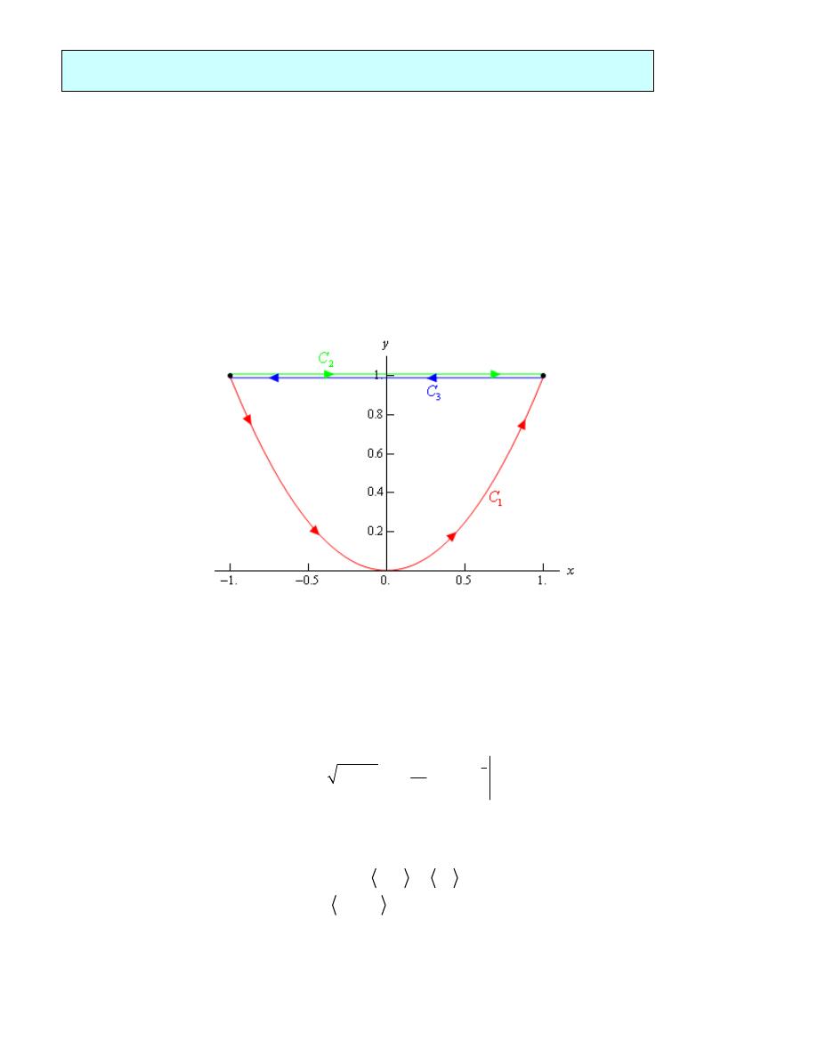
Example 1
Use Green’s Theorem to evaluate
2
3
C
xy dx
x y dy
+
ò
Ñ
where C is the triangle with
vertices
( )
0, 0
,
( )
1, 0
,
( )
1, 2
with positive orientation.
Solution
Green’s Theorem and we can see that the following inequalities will define the region enclosed.
0
1
0
2
x
y
x
£ £
£ £
We can identify P and Q from the line integral. Here they are.
2
3
P
xy
Q
x y
=
=
So , using Green’s Theorem the line integral becomes,
2
3
3
1
2
3
0
0
2
2
C
D
x
xy dx
x y dy
xy
x dA
xy
x dy dx
+
=
-
=
-
ó
õ
ò
òò
ò
Ñ
1
2
4
0
0
1
5
2
0
1
6
3
0
1
2
8
2
4
2
3
3
2
3
x
xy
xy
dx
x
x dx
x
x
æ
ö
=
-
ç
÷
è
ø
=
-
æ
ö
=
-
ç
÷
è
ø
=
ó
ô
õ
ò
Page 14 of 21
Line Integral's
<<2013-2014>>
Dr.Eng Muhammad.A.R.yass
Example 2
Evaluate
3
3
C
y dx
x dy
-
ò
Ñ
where C is the positively oriented circle of radius 2
centered at the origin.
Solution
o
Let’s first identify P and Q from the line integral.
3
3
P
y
Q
x
=
= -
Now, using Green’s theorem on the line integral gives,
3
3
2
2
3
3
C
D
y dx
x dy
x
y dA
-
= -
-
ò
òò
Ñ
(
)
3
3
2
2
2
2
3
0
0
2
2
4
0
0
2
0
3
3
1
3
4
3
4
24
C
D
y dx
x dy
x
y
dA
r dr d
r
d
d
p
p
p
q
q
q
p
-
= -
+
= -
= -
= -
= -
ó
õ
ó
ô
õ
ò
òò
ò
ò
Ñ
Example 3
Evaluate
3
3
C
y dx
x dy
-
ò
Ñ
where C are the two circles of radius 2 and radius 1
centered at the origin with positive orientation.
(
)
3
3
2
2
2
2
3
1
0
2
2
4
1
0
3
3
1
3
4
C
D
y dx
x dy
x
y
dA
r dr d
r
d
p
p
q
q
-
= -
+
= -
= -
ó
õ
ó
ô
õ
ò
òò
ò
Ñ
Solution
2
0
15
3
4
45
2
d
p
q
p
= -
= -
ó
ô
õ
1
2
C
C
C
A
x dy
y dx
x dy
y dx
=
= -
=
-
ò
ò
ò
Ñ
Ñ
Ñ
Fact
Example 4
Use Green’s Theorem to find the area of a disk of radius a.
Solution
We can use either of the integrals above, but the third one is probably the easiest. So,
1
2
C
A
x dy
y dx
=
-
ò
Ñ
Page 15 of 21
Line Integral's
<<2013-2014>>
Dr.Eng Muhammad.A.R.yass
where C is the circle of radius a. So, to do this we’ll need a parameterization of C. This is,
cos
sin
0
2
x
a
t
y
a
t
t
p
=
=
£ £
The area is then,
(
)
(
)
(
)
2
2
0
0
2
2
2
2
2
0
2
2
0
2
1
2
1
cos
cos
sin
sin
2
1
cos
sin
2
1
2
C
A
x dy
y dx
a
t a
t dt
a
t
a
t dt
a
t
a
t dt
a dt
a
p
p
p
p
p
=
-
=
-
-
=
+
=
=
ò
ò
ò
ò
ò
Ñ
Page 16 of 21
Line Integral's
<<2013-2014>>
Dr.Eng Muhammad.A.R.yass
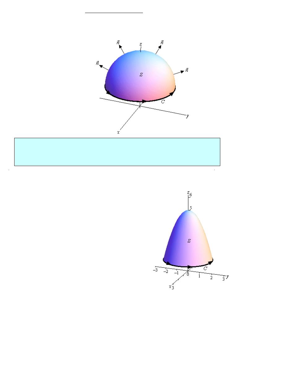
The following surface with the indicated orientation.
Stokes’ Theorem
Let S be an oriented smooth surface that is bounded by a simple, closed, smooth boundary curve
C with positive orientation. Also let
F
r
be a vector field then,
curl
C
S
F d r
F dS
=
ò
òò
r
r
r
r
g
g
Stokes' Theorm
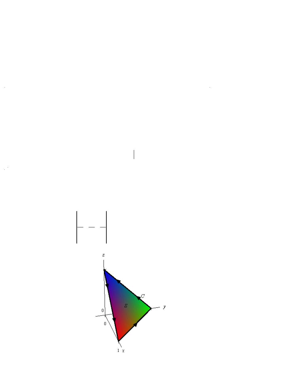
Example 1
Use Stokes’ Theorem to evaluate
curl
S
F dS
òò
r
r
g
where
2
3 3
3
F
z i
xy j x y k
=
-
+
r
r
r
r
and S is the part of
2
2
5
z
x
y
= -
-
above the plane
1
z
=
. Assume that S is oriented upwards.
Solution
Let’s start this off with a sketch of the surface.
In this case the boundary curve C will be where the surface intersects the plane
1
z
=
and so will
be the curve
2
2
2
2
1 5
4
at
1
x
y
x
y
z
= -
-
+
=
=
So, the boundary curve will be the circle of radius 2 that is in the plane
1
z
=
. The
parameterization of this curve is,
( )
2cos
2sin
, 0
2
r t
t i
t j k
t
p
=
+
+
£ £
r
r
r
r
Page 17 of 21
Line Integral's
<<2013-2014>>
Dr.Eng Muhammad.A.R.yass
The first two components give the circle and the third component makes sure that it is in the plane
1
z
=
.
Using Stokes’ Theorem we can write the surface integral as the following line integral.
( )
(
)
( )
2
0
curl
S
C
F dS
F d r
F r t
r t dt
p
¢
=
=
òò
ò
ò
r
r
r
r
r
r
r
g
g
g
So, it looks like we need a couple of quantities before we do this integral. Let’s first get the
vector field evaluated on the curve. Remember that this is simply plugging the components of the
parameterization into the vector field.
( )
(
)
( )
(
)(
) (
) (
)
2
3
3
3
3
1
3 2 cos
2sin
2cos
2sin
12 cos sin
64cos sin
F r t
i
t
t j
t
t k
i
t
t j
t
t k
=
-
+
= -
+
r
r
r
r
r
r
r
r
Next, we need the derivative of the parameterization and the dot product of this and the vector
field.
( )
( )
(
)
( )
2
2sin
2 cos
2sin
24sin cos
r t
t i
t j
F r t
r t
t
t
t
¢
= -
+
¢
= -
-
r
r
r
r r
r
g
We can now do the integral.
(
)
2
2
0
2
3
0
curl
2sin
24sin cos
2cos
8cos
0
S
F dS
t
t
t dt
t
t
p
p
=
-
-
=
+
=
òò
ò
r
r
g
Example 2
Use Stokes’ Theorem to evaluate
C
F d r
ò
r
r
g
where
2
2
F
z i
y j x k
=
+
+
r
r
r
r
and C is
the triangle with vertices
(
)
1,0,0
,
(
)
0,1,0
and
(
)
0,0,1
with counter-clockwise rotation.
Solution
We are going to need the curl of the vector field eventually so let’s get that out of the way first.
(
)
2
2
curl
2
2
1
i
j
k
F
z j
j
z
j
x
y
z
z
y
x
=
=
- =
-
r
r
r
r
r r
r
Page 18 of 21
Line Integral's
<<2013-2014>>

Dr.Eng Muhammad.A.R.yass
Since the plane is oriented upwards this induces the positive direction on C as shown. The
equation of this plane is,
( )
1
,
1
x y z
z g x y
x y
+ + =
Þ
=
= - -
Now, let’s use Stokes’ Theorem and get the surface integral set up.
(
)
(
)
curl
2
1
2
1
C
S
S
D
F d r
F dS
z
j dS
f
z
j
f dA
f
=
=
-
Ñ
=
-
Ñ
Ñ
ò
òò
òò
òò
r
r
r
r
g
g
r
r
g
r
g
Okay, we now need to find a couple of quantities. First let’s get the gradient. Recall that this
comes from the function of the surface.
(
)
( )
, ,
,
1
f x y z
z g x y
z
x y
f
i
j k
= -
= - + +
Ñ = + +
r
r r
Note as well that this also points upwards and so we have the correct direction.
Now, D is the region in the xy-plane shown below,
We get the equation of the line by plugging in
0
z
=
into the equation of the plane. So based on
this the ranges that define D are,
0
1
0
1
x
y
x
£ £
£ £ - +
The integral is then,
(
)
(
)
(
)
1
1
0
0
2
1
2 1
1
C
D
x
F d r
z
j i
j k dA
x y
dy dx
- +
=
-
+ +
=
- -
-
ò
òò
ò ò
r
r
r r r
r
g
g
Don’t forget to plug in for z since we are doing the surface integral on the plane. Finishing this
out gives,
(
)
1
1
0
0
1
1
2
0
0
1
2
0
1
3
2
0
1 2
2
2
1
1
3
2
1
6
x
C
x
F d r
x
y dy dx
y
xy y
dx
x
x dx
x
x
- +
- +
=
-
-
=
-
-
=
-
æ
ö
=
-
ç
÷
è
ø
= -
ò
ò ò
ò
ò
r r
g
Page 19 of 21
Line Integral's
<<2013-2014>>
Dr.Eng Muhammad.A.R.yass
Home Work
Page 20 of 21
Line Integral's
<<2013-2014>>
Dr.Eng Muhammad.A.R.yass
Page 21 of 21
Line Integral's
<<2013-2014>>