
2
nd
A
d
Clas
M
Adva
s
Uni
Electro
Mult
anc
iversity of
omechani
Energy
tipl
ed
f Technolo
cal Depar
Branch
le In
Ma
ogy
tment
nteg
athe
gra
ema
al
atic
2
st
Le
cs
cture

Dr.Eng Muhammad.A.R.yass
Advance Mathematic
Multiple Integral
2 Class Electromechanical Engineer
nd
Dr.Eng.Muhammad.A.R.Yass
by
multiple Integral
1 of 39
<<2013-2014>>

Dr.Eng Muhammad.A.R.yass
Multiple Integral
Double Integral
Iterated Integrals
Double Integral Over General Regions
Double Integral in Polar Coordinates
Triple Integrals
Triple Integral inCylindrical Coordinates
Triple Integrals in Sperical coordinates
Change of Variables
Surface Area
Area and Volume Revisited
multiple Integral
2 of 39
<<2013-2014>>
Dr.Eng Muhammad.A.R.yass
Double Integrals
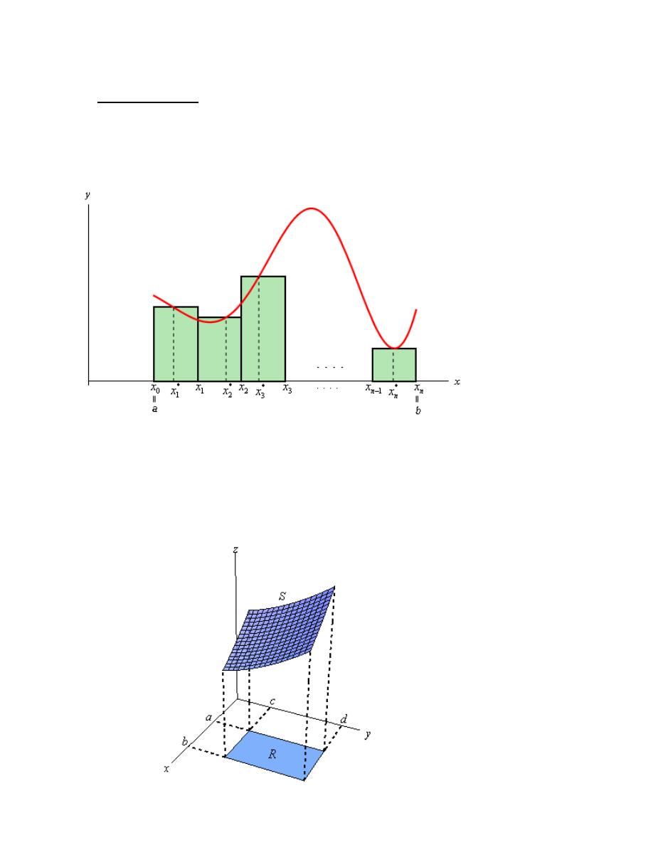
definition of a definite integrals for functions of single variables
( )
b
a
f x dx
∫
b
x
a
≤ ≤
.
( )
( )
*
1
lim
n
b
i
a
n
i
f x dx
f x
x
→∞ =
=
∆
∑
∫
Double Integrals
The
and
also
We will start out by assuming that the region in
2
¡
is a rectangle which we will denote as
follows,
[ ] [ ]
,
,
R
a b
c d
=
×
This means that the ranges for x and y are
a
x
b
≤ ≤
and
c
y
d
≤ ≤
.
Also, we will initially assume that
( )
,
0
f x y
≥
although this doesn’t really have to be the case.
multiple Integral
3 of 39
<<2013-2014>>
Dr.Eng Muhammad.A.R.yass
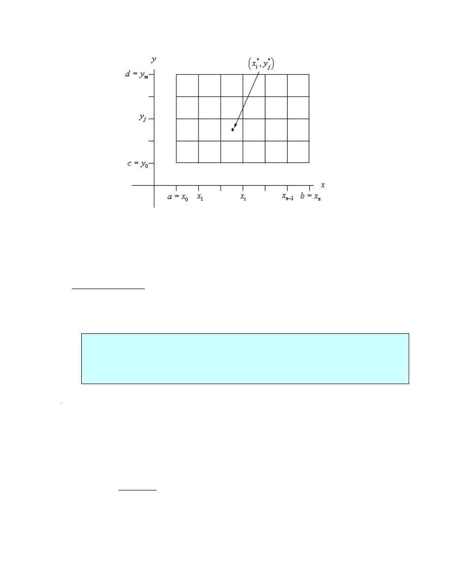
Here is the official definition of a double integral of a function of two variables over a rectangular
region R as well as the notation that we’ll use for it.
( )
(
)
*
*
,
1
1
,
lim
,
n
m
i
j
n m
i
j
R
f x y dA
f x y
A
→∞
=
=
=
∆
∑∑
∫∫
Iterated Integrals
The following theorem tells us how to compute a double integral over a rectangle.
Fubini’s Theorem
If
( )
,
f x y
is continuous on
[ ] [ ]
,
,
R
a b
c d
=
×
then,
( )
( )
( )
,
,
,
R
b
d
d
b
c
a
a
c
f x y dA
f x y dy dx
f x y dx dy
=
=
⌠
⌠
⌡
⌡
∫∫
∫
∫
These integrals are called iterated integrals.
Example 1
Compute each of the following double integrals over the indicated rectangles.
(a)
2
6
R
xy dA
∫∫
,
[ ] [ ]
2, 4
1, 2
R
=
×
(b)
3
2
4
R
x
y dA
−
∫∫
,
[
] [ ]
5, 4
0,3
R
= −
×
(c)
( )
( )
2
2
cos
sin
R
x y
x
y dA
π
π
+
+
∫∫
,
[
] [ ]
2, 1
0,1
R
= − − ×
(d)
(
)
2
1
2
3
R
dA
x
y
+
⌠⌠
⌡⌡
,
[ ] [ ]
0,1
1, 2
R
=
×
(e)
R
xy
x
dA
∫∫
e
,
[
] [ ]
1, 2
0,1
R
= −
×
multiple Integral
4 of 39
<<2013-2014>>

Dr.Eng Muhammad.A.R.yass
Solution
(a)
2
6
R
xy dA
∫∫
,
[ ] [ ]
2, 4
1, 2
R
=
×
Solution 1
In this case we will integrate with respect to y first. So, the iterated integral that we need to
compute is,
2
2
4
2
1
2
6
6
R
xy dA
xy dy dx
= ⌠
⌡
∫∫
∫
( )
2
2
3
1
4
2
4
2
4
2
6
2
16
2
14
R
xy dA
xy
dx
x
x dx
x dx
=
=
−
=
⌠
⌡
∫∫
∫
∫
4
2
2
2
6
7
84
R
xy dA
x
=
=
∫∫
Solution 2
In this case we’ll integrate with respect to x first and then y. Here is the work for this solution.
(
)
2
2
4
2
2
2
2
2
3
1
2
4
2
1
2
1
2
1
6
6
3
36
12
84
R
xy dA
xy dx dy
x y
dy
y dy
y
=
=
=
=
=
⌠
⌡
⌠
⌡
∫∫
∫
∫
(b)
3
2
4
R
x
y dA
−
∫∫
,
[
] [ ]
5, 4
0, 3
R
= −
×
For this integral we’ll integrate with respect to y first.
(
)
3
3
3
4
0
4
3
0
5
4
5
4
5
2
4
2
4
2
6
81
R
x
y dA
x
y dy dx
xy
y
dx
x
dx
−
−
−
−
=
−
=
−
=
−
⌠
⌡
⌠
⌡
∫∫
∫
∫
(
)
4
2
5
3
81
756
x
x
−
=
−
= −
multiple Integral
5 of 39
<<2013-2014>>

Dr.Eng Muhammad.A.R.yass
( )
( )
( )
( )
( )
( )
( )
( )
2
2
2
2
1
3
2
2
2
1
3
0
1
1
2
0
1
0
1
0
cos
sin
cos
sin
1
1
sin
sin
3
7
sin
3
7
1
cos
9
7
2
9
R
x y
x
y dA
x y
x
y dx dy
x y
x
x
y
dy
y
y dy
y
y
π
π
π
π
π
π
π
π
π
π
π
−
−
−
−
+
+
=
+
+
=
+
+
=
+
=
−
= +
⌠
⌡
⌠
⌡
⌠
⌡
∫∫
∫
(d)
(
)
2
1
2
3
R
dA
x
y
+
⌠⌠
⌡⌡
,
[ ] [ ]
0,1
1, 2
R
=
×
(
)
(
)
(
)
(
)
2
2
1
1
0
2
1
2
1
0
1
2
1
2
1
2
3
2
3
1
2
3
2
1
1
1
2
2 3
3
1 1
1
ln 2 3
ln
2 3
3
1
ln 8 ln 2 ln 5
6
R
x
y
dA
x
y
dx dy
x
y
dy
dy
y
y
y
y
−
−
−
+
=
+
=
−
+
= −
−
+
= −
+
−
= −
−
−
⌠
⌡
⌠
⌡
⌠
⌡
∫∫
∫
(e)
R
xy
x
dA
∫∫
e
,
[
] [ ]
1, 2
0,1
R
= −
×
(c)
( )
( )
2
2
cos
sin
R
x y
x
y dA
π
π
+
+
∫∫
,
[
] [ ]
2, 1
0,1
R
= − − ×
2
1
1 0
R
xy
xy
x
dA
x
dy dx
−
=
∫∫
∫ ∫
e
e
be done with the quick substitution,
u
xy
du
x dy
=
=
2
1
0
1
2
1
R
xy
xy
x
x
dA
dx
dx
−
−
=
=
−
∫∫
∫
∫
e
e
e
(
)
(
)
1
2
1
2
1
2
1
2
1
3
x
x
−
−
−
=
−
= − −
+
= −
−
e
e
e
e
e
multiple Integral
6 of 39
<<2013-2014>>
Dr.Eng Muhammad.A.R.yass
1
2
0
1
R
xy
xy
x
dA
x
dx dy
−
=
∫∫
∫ ∫
e
e
In order to do this we would have to use integration by parts as follows,
1
xy
xy
u
x
dv
dx
du
dx
v
y
=
=
=
=
e
e
The integral is then,
1
2
1
0
1
2
2
1
0
1
2
2
0
2
2
1
1
2
1
1
1
R
xy
xy
xy
xy
xy
y
y
y
y
x
x
dA
dx
dy
y
y
x
dy
y
y
dy
y
y
y
y
−
−
−
−
=
−
=
−
=
−
− −
−
⌠
⌠
⌡
⌡
⌠
⌡
⌠
⌡
∫∫
e
e
e
e
e
e
e
e
e
If we change the order from dydx to dxdy the solution will be more difficult see that
difficult to continue
Fact
If
( )
( ) ( )
,
f x y
g x h y
=
and we are integrating over the rectangle
[ ] [ ]
,
,
R
a b
c d
=
×
then,
( )
( ) ( )
( )
(
)
( )
(
)
,
R
R
b
d
a
c
f x y dA
g x h y dA
g x dx
h y dy
=
=
∫∫
∫∫
∫
∫
Example 2
Evaluate
( )
2
cos
R
x
y dA
∫∫
,
[
]
2, 3
0,
2
R
π
= −
×
.
Solution
Since the integrand is a function of x times a function of y we can use the fact.
( )
(
)
( )
( )
( )
2
2
3
2
2
2
0
3
2
2
0
2
0
cos
cos
1
1
1 cos 2
2
2
5
1
1
sin 2
2
2
2
5
R
x
y dA
x dx
y dy
x
y dy
y
y
π
π
π
π
−
−
=
=
+
=
+
=
∫∫
∫
∫
∫
8
multiple Integral
7 of 39
<<2013-2014>>
Dr.Eng Muhammad.A.R.yass
Double Integrals Over General Regions
In the previous section we looked at double integrals over rectangular regions. The problem with
this is that most of the regions are not rectangular so we need to now look at the following double
integral,
( )
,
D
f x y dA
∫∫
where D is any region.
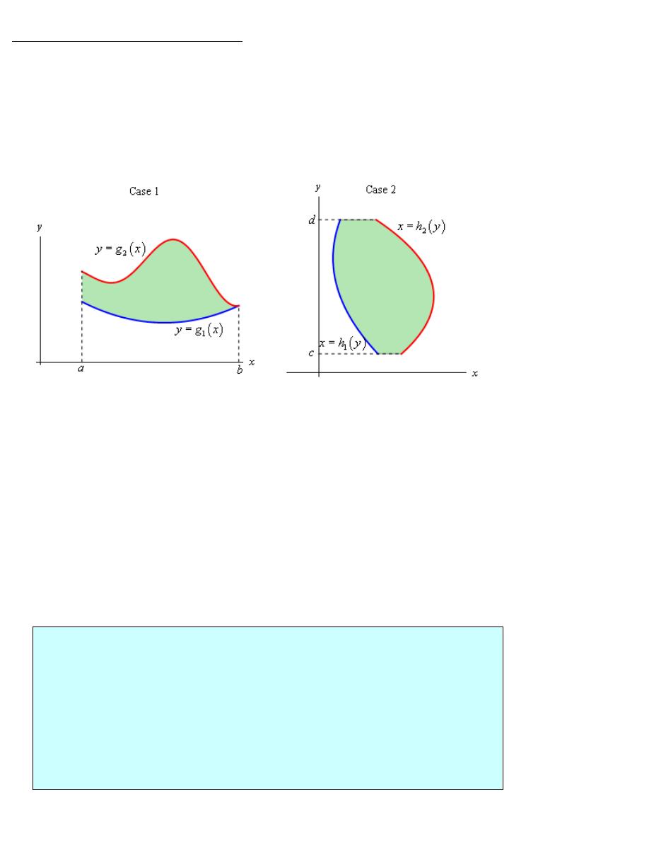
There are two types of regions that we need to look at. Here is a sketch of both of them.
Case 1
( )
( )
( )
{
}
1
2
,
|
,
D
x y
a
x
b g x
y
g
x
=
≤ ≤
≤ ≤
Case 2.
( ) ( )
( )
{
}
1
2
,
|
,
D
x y
h y
x
h
y c
y
d
=
≤ ≤
≤ ≤
In Case 1 where
( )
( )
( )
{
}
1
2
,
|
,
D
x y
a
x
b g x
y
g
x
=
≤ ≤
≤ ≤
the integral is defined to be,
( )
( )
( )
( )
2
1
,
,
D
b
g
x
g
x
a
f x y dA
f x y dy dx
= ⌠
⌡
∫∫
∫
In Case 2 where
( ) ( )
( )
{
}
1
2
,
|
,
D
x y
h y
x
h
y c
y
d
=
≤ ≤
≤ ≤
the integral is defined to be,
( )
( )
( )
( )
2
1
,
,
D
d
h
y
h y
c
f x y dA
f x y dx dy
= ⌠
⌡
∫∫
∫
P
ropert
i
es
1.
( ) ( )
( )
( )
,
,
,
,
D
D
D
f x y
g x y dA
f x y dA
g x y dA
+
=
+
∫∫
∫∫
∫∫
2.
( )
( )
,
,
D
D
cf x y dA
c
f x y dA
=
∫∫
∫∫
, where c is any constant.
3.
If the region D can be split into two separate regions D
1
and D
2
then the integral can be written
as
( )
( )
( )
1
2
,
,
,
D
D
D
f x y dA
f x y dA
f x y dA
=
+
∫∫
∫∫
∫∫
multiple Integral
8 of 39
<<2013-2014>>
Dr.Eng Muhammad.A.R.yass
Example 1
Evaluate each of the following integrals over the given region D.
(a)
x
y
D
dA
⌠⌠
⌡⌡
e
,
( )
{
}
3
,
|1
2,
D
x y
y
y
x
y
=
≤ ≤
≤ ≤
(b)
3
4
D
xy
y dA
−
∫∫
, D is the region bounded by
y
x
=
and
3
y
x
=
.
(c)
2
6
40
D
x
y dA
−
∫∫
, D is the triangle with vertices
( )
0, 3
,
( )
1,1
, and
( )
5, 3
.
Solution
(a)
x
y
D
dA
⌠⌠
⌡⌡
e
,
( )
{
}
3
,
|1
2,
D
x y
y
y
x
y
=
≤ ≤
≤ ≤
Okay, this first one is set up to just use the formula above so let’s do that.
3
3
2
2
2
2
1
1
2
1
1
2
2 1
4
1
1
1
1
1
2
2
2
2
y
x
x
x
y
y
y
D
y
y
y
y
y
dA
dx dy
y
dy
y
y dy
y
=
=
=
−
=
−
=
−
⌠
⌠
⌠⌠
⌠
⌡⌡
⌡
⌡
⌡
∫
e
e
e
e
e
e
e
e
e
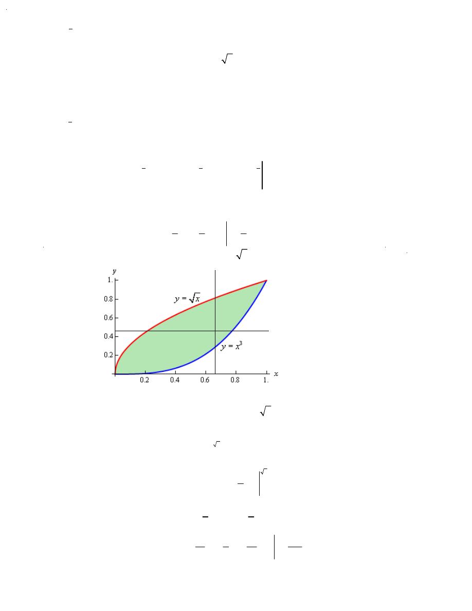
(b)
3
4
D
xy
y dA
−
∫∫
, D is the region bounded by
y
x
=
and
3
y
x
=
.
So, from the sketch we can see that that two inequalities are,
3
0
1
x
x
y
x
≤ ≤
≤ ≤
We can now do the integral,
3
3
1
3
3
0
1
2
4
0
4
4
1
2
4
D
x
x
x
x
xy
y dA
xy
y dy dx
xy
y
dx
−
=
−
=
−
⌠
⌡
⌠
⌡
∫∫
∫
1
2
7
12
0
1
3
8
13
0
7
1
2
4
4
7
1
1
55
12
4
52
156
x
x
x dx
x
x
x
=
−
+
=
−
+
=
⌠
⌡
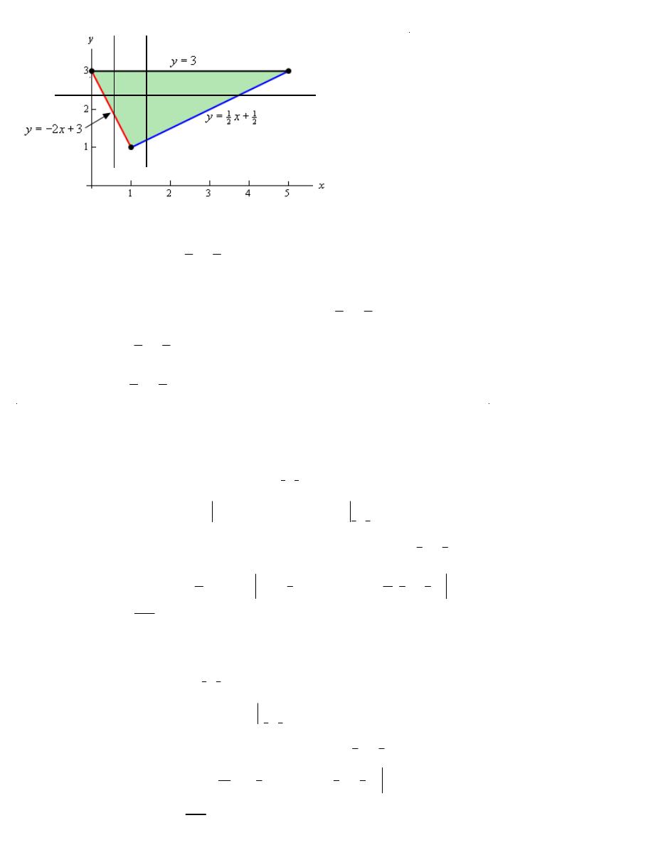
(c)
2
6
40
D
x
y dA
−
∫∫
, D is the triangle with vertices
( )
0, 3
,
( )
1,1
, and
5,3
.
Projection for (dy dx)
Projection fo (dx dy)
multiple Integral
9 of 39
<<2013-2014>>
Dr.Eng Muhammad.A.R.yass
( )
{
}
( )
1
2
,
| 0
1,
2
3
3
1
1
,
|1
5,
3
2
2
D
x y
x
x
y
D
x y
x
x
y
=
≤ ≤ −
+ ≤ ≤
=
≤ ≤
+ ≤ ≤
To avoid this we could turn things around and solve the two equations for x to get,
1
3
2
3
2
2
1
1
2
1
2
2
y
x
x
y
y
x
x
y
= − +
⇒
= −
+
=
+
⇒
=
−
( )
1
3
,
|
2
1, 1
3
2
2
D
x y
y
x
y
y
=
−
+ ≤ ≤
−
≤ ≤
Projection for (dy dx)
(Two)
Projection fo (dx dy)
(one)
Solution 1
(
)
(
)
(
)
(
)
1
2
2
2
2
5
1
3
3
2
2
1
1
2
3
0
1
2
2
5
1
3
3
2
2
2
2
1
1
2
3
0
1
2
2
1
5
2
2
3
3
2
1
1
2
2
0
1
6
40
6
40
6
40
6
40
6
40
6
20
6
20
12
180
20 3 2
3
15
180
20
D
D
D
x
x
x
x
x
y dA
x
y dA
x
y dA
x
y dy dx
x
y dy dx
x y
y
dx
x y
y
dx
x
x
dx
x
x
x
dx
− +
+
− +
+
−
=
−
+
−
=
−
+
−
=
−
+
−
=
−
+
−
+ −
+
−
+
+
⌠
⌠
⌡
⌡
⌠
⌠
⌡
⌡
∫∫
∫∫
∫∫
∫
∫
∫
∫
5
1
4
10
3
3
180
3
x
x
=
−
−
−
(
)
(
)
(
)
(
)
3
3
4
3
3
40
1
1
4
3
2
2
0
1
2
5
180
935
3
x
x
x
x
x
+ −
+
−
+
+
= −
Solution 2
This solution will be a lot less work since we are only going to do a single integral.
(
)
(
)
(
)
(
)
(
)
(
)
3
2
1
2
2
1
3
1
2
2
3
2
1
3
1
3
1
2
2
3
3
3
2
3
1
2
2
1
3
4
4
2
3
100
3
1
1
3
4
2
2
1
6
40
6
40
2
40
100
100
2 2
1
2
50
2
1
935
3
y
y
D
y
y
x
y dA
x
y dx dy
x
xy
dy
y
y
y
y
dy
y
y
y
y
−
−
+
−
−
+
−
=
−
=
−
=
−
+
−
− −
+
=
−
+
−
+ −
+
= −
⌠
⌡
⌠
⌡
∫∫
∫
∫
multiple Integral
10 of 39
<<2013-2014>>
Dr.Eng Muhammad.A.R.yass
Example 2
Evaluate the following integrals by first reversing the order of integration.
(a)
3
2
3
9
3
0
y
x
x
dy dx
⌠
⌡
∫
e
(b)
3
8
2
4
0
1
y
x
dx dy
+
⌠
⌡
∫
Solution
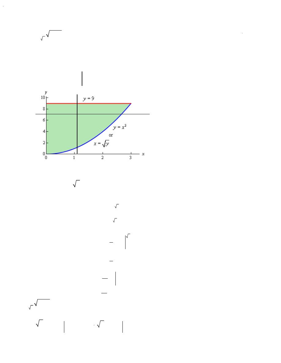
(a)
3
2
3
9
3
0
y
x
x
dy dx
⌠
⌡
∫
e
2
0
3
9
x
x
y
≤ ≤
≤ ≤
0
0
9
x
y
y
≤ ≤
≤ ≤
that mean x=0, x=3
that mean y=9, y=x
2
from this value we draw the graph as shown
so the limits for dxdy
The integral, with the order reversed, is now,
3
3
2
9
3
9
3
3
0
0
0
y
y
y
x
x
dy dx
x
dx dy
= ⌠
⌠
⌡
⌡
∫
∫
e
e
3
3
3
3
3
2
9
3
9
3
3
0
0
0
9
4
0
0
9
2
0
9
0
1
4
1
4
1
12
y
y
y
y
y
y
y
x
x
dy dx
x
dx dy
x
dy
y
dy
=
=
=
=
⌠
⌠
⌡
⌡
⌠
⌡
⌠
⌡
∫
∫
e
e
e
e
e
(
)
729
1
1
12
=
−
e
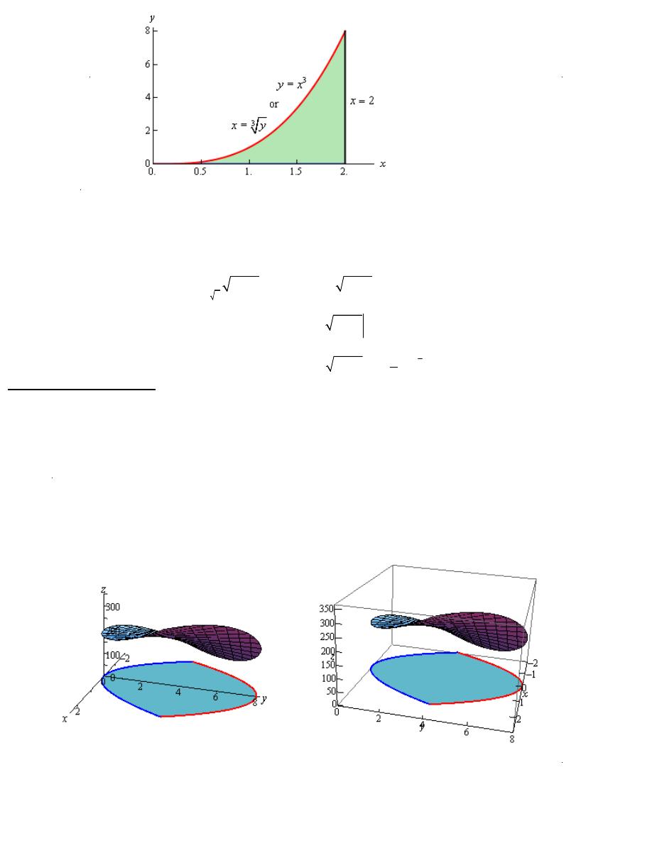
(b)
3
8
2
4
0
1
y
x
dx dy
+
⌠
⌡
∫
3
2
0
8
y
x
y
≤ ≤
≤ ≤
That mean x = y ,x=2
3
That mean y=0 , y= 8
so the graph will be
multiple Integral
11 of 39
<<2013-2014>>
Dr.Eng Muhammad.A.R.yass
Calculus III
So, if we reverse the order of integration we get the following limits.
3
0
2
0
x
y
x
≤ ≤
≤ ≤
The integral is then,
3
3
3
2
8
2
4
4
0
0
0
2
4
0
0
3
2
3
4
2
0
1
1
1
1
1
17
1
6
x
x
y
x
dx dy
x
dy dx
y x
dx
x
x
dx
+
=
+
=
+
=
+
=
−
⌠
⌠
⌡
⌡
⌠
⌡
∫
∫
∫
The volume of the solid that lies below the surface given by
( )
,
z
f x y
=
and above the region D
in the xy-plane is given by,
( )
,
D
V
f x y dA
=
∫∫
The Volume of Solid
Example 3
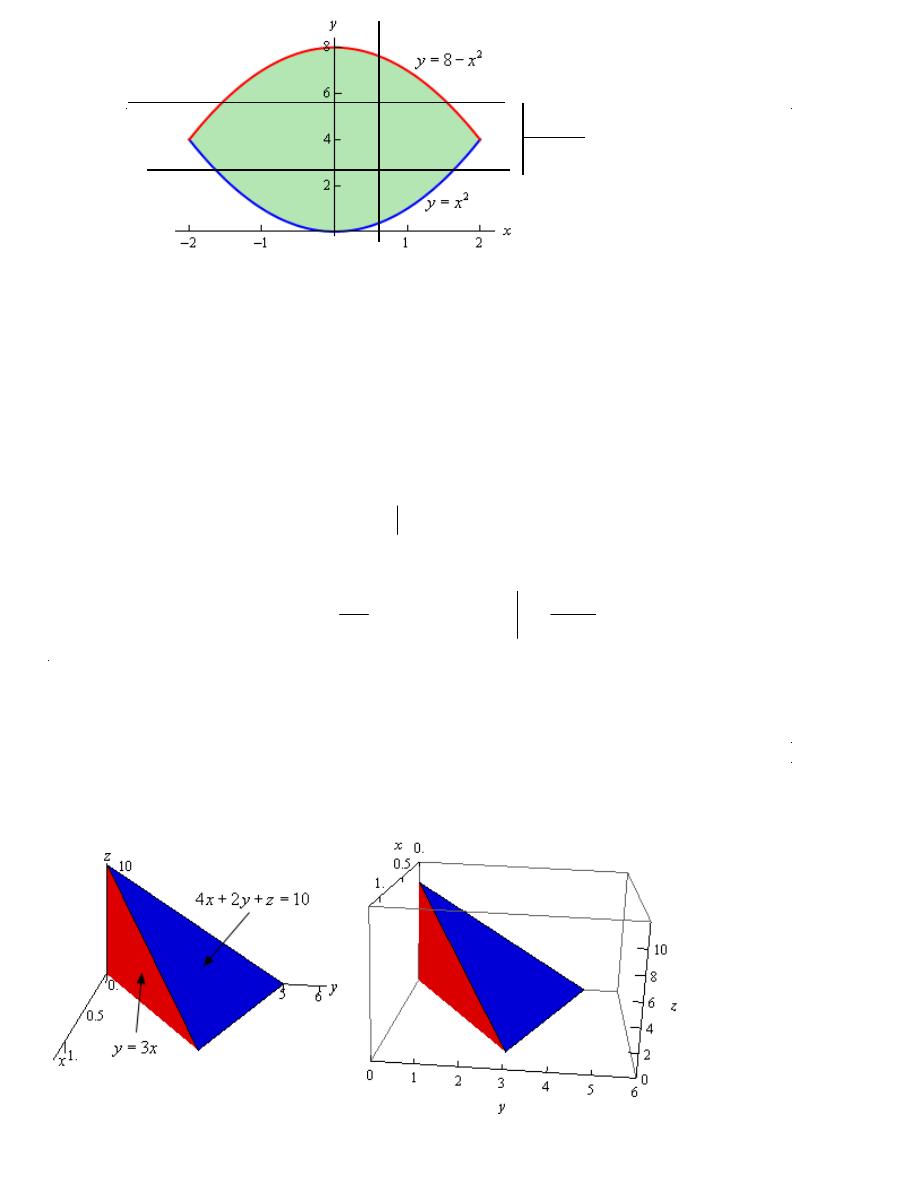
Find the volume of the solid that lies below the surface given by
16
200
z
xy
=
+
and lies above the region in the xy-plane bounded by
2
y
x
=
and
2
8
y
x
= −
.
Solution
Here is the graph of the surface and we’ve tried to show the region in the xy-plane below the
surface.
Here is a sketch of the region in the xy-plane by itself.
multiple Integral
12 of 39
<<2013-2014>>
Dr.Eng Muhammad.A.R.yass
By setting the two bounding equations equal we can see that they will intersect at
2
x
=
and
2
x
= −
. So, the inequalities that will define the region D in the xy-plane are,
2
2
2
2
8
x
x
y
x
− ≤ ≤
≤ ≤ −
The volume is then given by,
(
)
2
2
2
2
2
8
2
2
8
2
2
2
3
2
2
2
4
3
2
2
16
200
16
200
8
200
128
400
512
1600
400
12800
32
256
1600
3
3
D
x
x
x
x
V
xy
dA
xy
dy dx
xy
y
dx
x
x
x
dx
x
x
x
x
−
−
−
−
−
−
=
+
=
+
=
+
=
−
−
+
+
= −
−
+
+
=
⌠
⌡
⌠
⌡
∫∫
∫
∫
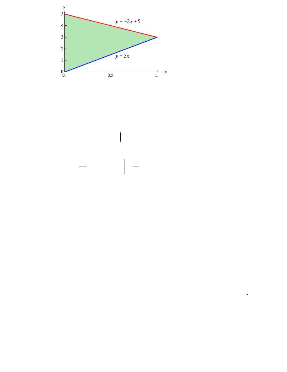
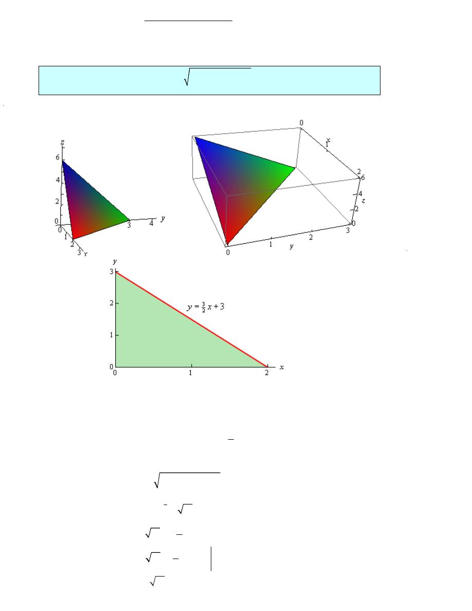
Example 4
Find the volume of the solid enclosed by the planes
4
2
10
x
y
z
+
+ =
,
3
y
x
=
,
0
z
=
,
0
x
=
.
Solution
The first plane,
4
2
10
x
y
z
+
+ =
,
10 4
2
z
x
y
= −
−
. The second plane,
3
y
x
=
So
0 4
2
10
2
5
2
5
x
y
x
y
y
x
+
+
=
⇒
+ =
⇒
= − +
o, here is a sketch the region D.
projection for (dydx)
projection for (dxdy)
(not possible)
multiple Integral
13 of 39
<<2013-2014>>
Dr.Eng Muhammad.A.R.yass
,
0
1
3
2
5
x
x
y
x
≤ ≤
≤ ≤ − +
(
)
1
0
1
2
5
2
3
0
1
2
0
1
3
2
0
2
5
3
10 4
2
10 4
2
10
4
25
50
25
25
25
25
25
3
3
D
x
x
x
x
V
x
y dA
x
y dy dx
y
xy
y
dx
x
x
dx
x
x
x
− +
− +
=
−
−
=
−
−
=
−
−
=
−
+
=
−
+
=
⌠
⌡
∫∫
∫ ∫
∫
multiple Integral
14 of 39
<<2013-2014>>
Dr.Eng Muhammad.A.R.yass
26
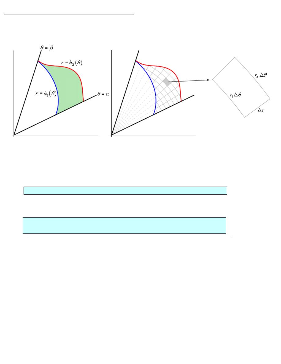
Double Integral in Polar Coordinates
a general region in terms of polar coordinates and see what we can do with that
. Here is a sketch of some region using polar coordinates.
So, our general region will be defined by inequalities,
( )
( )
1
2
h
r
h
α θ β
θ
θ
≤ ≤
≤ ≤
Now, to find dA let’s redo the figure above as follows,
dA
r dr d
θ
=
2
2
2
cos
sin
x
r
y
r
r
x
y
θ
θ
=
=
=
+
( )
(
)
( )
( )
2
1
,
cos , sin
h
h
D
f x y dA
f r
r
r dr d
β
θ
θ
α
θ
θ
θ
= ⌠
⌡
∫∫
∫
Example 1
Evaluate the following integrals by converting them into polar coordinates.
(a)
2
D
x y dA
∫∫
, D is the portion of the region between the circles of radius 2
and radius 5 centered at the origin that lies in the first quadrant.
(b)
2
2
D
x
y
dA
+
∫∫
e
, D is the unit circle centered at the origin.
Solution
(a)
2
D
x y dA
∫∫
, D is the portion of the region between the circles of radius 2 and radius 5
centered at the origin that lies in the first quadrant.
First let’s get D in terms of polar coordinates. The circle of radius 2 is given by
2
r
=
and the
circle of radius 5 is given by
5
r
=
. We want the region between them so we will have the
following inequality for r
2
5
r
≤ ≤
Also
,
since
we
only
want
the
portion
that
is
in
the
first
quadrant
we
get
the
following
range
of
θ
’s.
multiple Integral
15 of 39
<<2013-2014>>

Dr.Eng Muhammad.A.R.yass
0
2
π
θ
≤ ≤
Now that we’ve got these we can do the integral.
(
)(
)
5
2
2
0
2
2
cos
sin
D
x y dA
r
r
r dr d
π
θ
θ
θ
= ⌠
⌡
∫∫
∫
Don’t forget to do the conversions and to add in the extra r. Now, let’s simplify and make use of
the double angle formula for sine to make the integral a little easier.
( )
( )
( )
5
2
3
2
0
5
2
4
2
0
2
0
2
sin 2
1
sin 2
4
609
sin 2
4
D
x y dA
r
dr d
r
d
d
π
π
π
θ
θ
θ
θ
θ θ
=
=
=
⌠
⌡
⌠
⌡
⌠
⌡
∫∫
∫
( )
2
0
609
cos 2
8
π
θ
= −
609
4
=
(b)
2
2
D
x
y
dA
+
∫∫
e
, D is the unit circle centered at the origin.
In this case we can’t do this integral in terms of Cartesian coordinates. We will however be able
to do it in polar coordinates. First, the region D is defined by,
0
2
0
1
r
θ
π
≤ ≤
≤ ≤
In terms of polar coordinates the integral is then,
2
2
2
2
1
0
0
D
x
y
r
dA
r
dr d
π
θ
+
= ⌠
⌡
∫∫
∫
e
e
Notice that the addition of the r gives us an integral that we can now do. Here is the work for this
integral.
2
2
2
2
1
0
0
D
x
y
r
dA
r
dr d
π
θ
+
= ⌠
⌡
∫∫
∫
e
e
(
)
(
)
2
2
1
0
0
2
0
1
2
1
1
2
1
r
d
d
π
π
θ
θ
π
=
=
−
=
−
⌠
⌡
⌠
⌡
e
e
e
multiple Integral
16 of 39
<<2013-2014>>
Dr.Eng Muhammad.A.R.yass
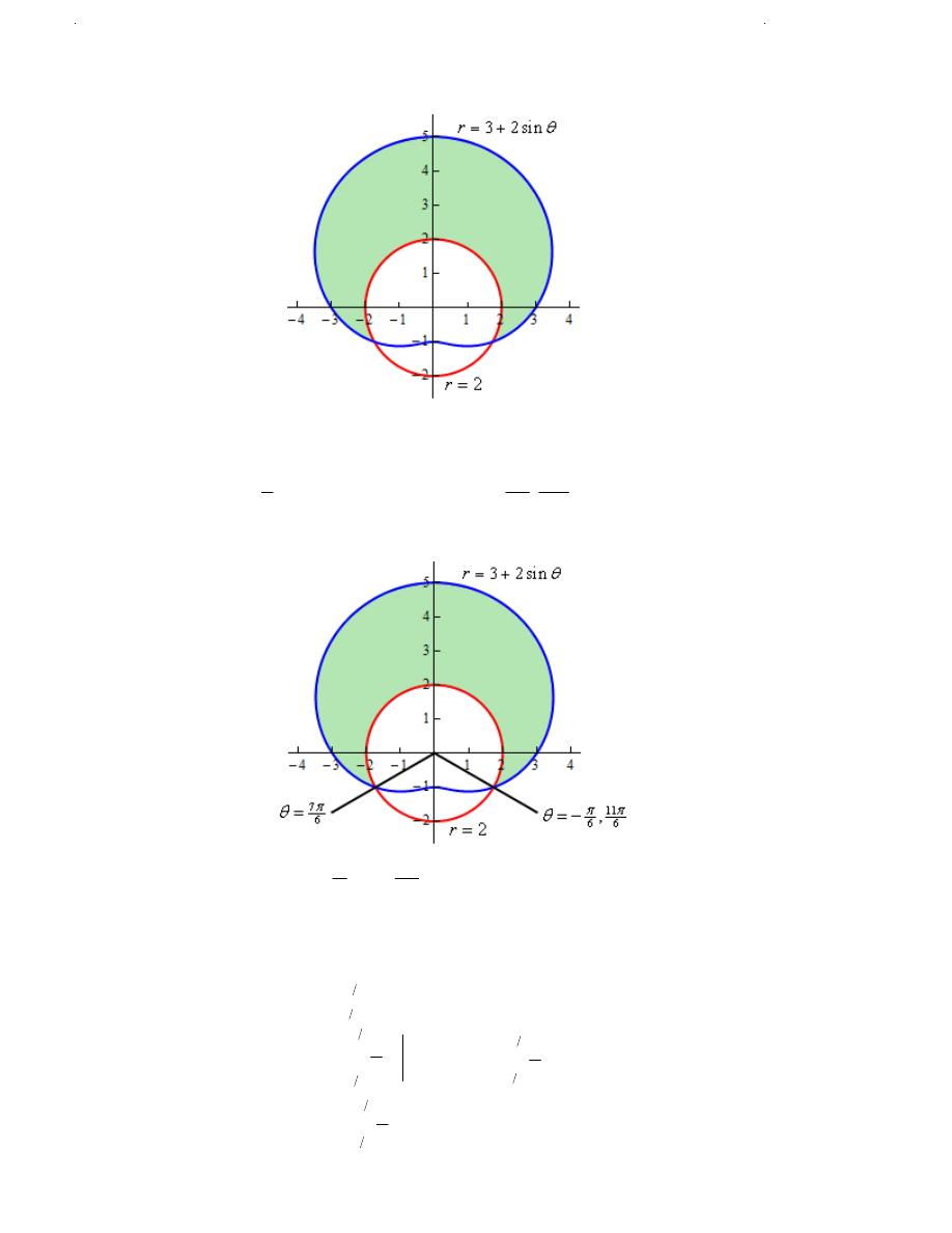
Example 2
Determine the area of the region that lies inside
3 2sin
r
θ
= +
and outside
2
r
=
.
Solution
Here is a sketch of the region, D, that we want to determine the area of.
by setting the two equations and solving.
3 2 sin
2
1
7
11
sin
,
2
6
6
θ
π
π
θ
θ
+
=
= −
⇒
=
Here is a sketch of the figure with these angles added.
So, here are the ranges that will define the region.
7
6
6
2
3 2 sin
r
π
π
θ
θ
− ≤ ≤
≤ ≤ +
( )
7
6
3 2sin
6
2
7
6
3 2sin
2
2
6
7
6
2
6
7
6
6
1
2
5
6 sin
2 sin
2
7
6 sin
cos 2
2
D
A
dA
r drd
r
d
d
d
π
θ
π
π
θ
π
π
π
π
π
θ
θ
θ
θ θ
θ
θ θ
+
−
+
−
−
−
=
=
=
=
+
+
=
+
−
⌠
⌡
⌠
⌡
⌠
⌡
∫∫
∫ ∫
multiple Integral
17 of 39
<<2013-2014>>
Dr.Eng Muhammad.A.R.yass
( )
7
6
6
7
1
6 cos
sin 2
2
2
11 3
14
24.187
2
3
π
π
θ
θ
θ
π
−
=
−
−
=
+
=
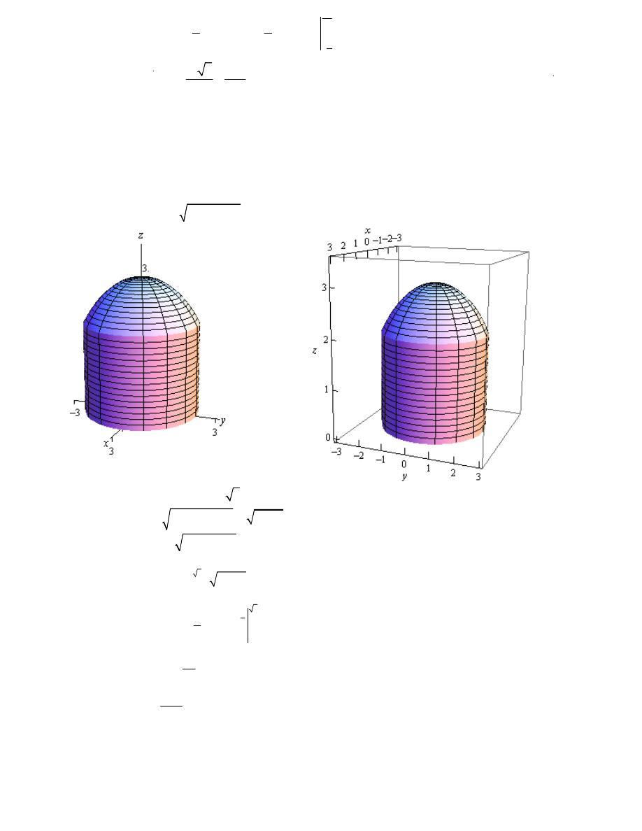
Example 3
Determine the volume of the region that lies under the sphere
2
2
2
9
x
y
z
+
+
=
,
above the plane
0
z
=
and inside the cylinder
2
2
5
x
y
+
=
.
Solution
We know that the formula for finding the volume of a region is,
( )
,
D
V
f x y dA
=
∫∫
Here is the function.
2
2
9
z
x
y
=
− −
( )
,
f x y
As we know that z=
0
2
0
5
r
θ
π
≤ ≤
≤ ≤
(
)
2
2
2
9
9
z
x
y
r
=
−
+
=
−
(
)
2
2
2
5
2
0
0
2
5
3
2
2
0
0
9
9
1
9
3
D
V
x
y dA
r
r dr d
r
d
π
π
θ
θ
=
− −
=
−
=
−
−
⌠
⌡
⌠
⌡
∫∫
∫
2
0
19
3
38
3
d
π
θ
π
=
=
⌠
⌡
multiple Integral
18 of 39
<<2013-2014>>
Dr.Eng Muhammad.A.R.yass
( )
,
D
V
f x y dA
=
∫∫
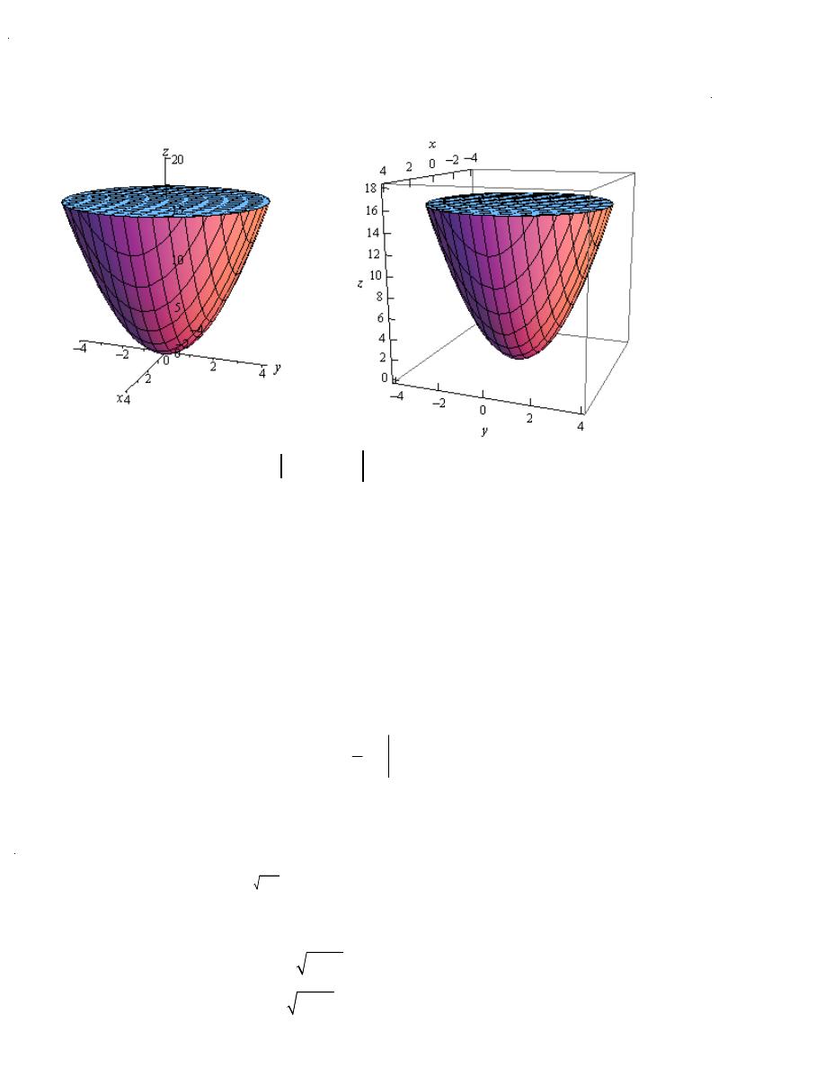
Example 4
Find the volume of the region that lies inside
2
2
z
x
y
=
+
and below the plane
16
z
=
.
Solution
Let’s start this example off with a quick sketch of the region.
( )
,
D
f x y
=
∫∫
upper
-
( )
,
f x y
Lower
dA
{
}
2
2
16
D
V
x
y
dA
=
−
+
∫∫
so
(
)
{
(
) }
.
2
0
2
0
4
16
r
z
r
θ
π
≤ ≤
≤ ≤
= −
me is then,
(
)
(
)
2
2
2
4
2
0
0
4
2
2
4
0
0
16
16
1
8
4
D
V
x
y
dA
r
r
dr d
r
r
d
π
π
θ
θ
=
−
+
=
−
=
−
⌠
⌡
⌠
⌡
∫∫
∫
2
0
64
128
d
π
θ
π
=
=
∫
Example 5
Evaluate the following integral by first converting to polar coordinates.
(
)
2
1
1
2
2
0
0
cos
y
x
y
dx dy
−
+
⌠
⌡
∫
Solution
2
0
1
0
1
y
x
y
≤ ≤
≤ ≤
−
2
1
x
y
=
−
multiple Integral
19 of 39
<<2013-2014>>

Dr.Eng Muhammad.A.R.yass
0
2
0
1
r
π
θ
≤ ≤
≤ ≤
dx dy
dA
r dr d
θ
=
=
and so the integral becomes,
(
)
( )
2
1
1
1
2
2
2
2
0
0
0
0
cos
cos
y
x
y
dx dy
r
r
dr d
π
θ
−
+
=
⌠
⌡
∫
∫ ∫
Note that this is an integral that we can do. So, here is the rest of the work for this integral.
(
)
( )
( )
( )
2
1
1
2
1
2
2
2
0
0
0
0
2
0
1
cos
sin
2
1
sin 1
2
sin 1
4
y
x
y
dx dy
r
d
d
π
π
θ
θ
π
−
+
=
=
=
⌠
⌠
⌡
⌡
⌠
⌡
∫
multiple Integral
20 of 39
<<2013-2014>>
Dr.Eng Muhammad.A.R.yass
The notation for the general triple integrals is,
(
)
, ,
E
f x y z dV
∫∫∫
Let’s start simple by integrating over the box,
[ ] [ ] [ ]
,
,
,
B
a b
c d
r s
=
×
×
Note that when using this notation we list the x’s first, the y’s second and the z’s third.
The triple integral in this case is,
(
)
(
)
, ,
, ,
B
s
d
b
r
c
a
f x y z dV
f x y z dx dy dz
=
∫∫∫
∫ ∫ ∫
Example 1
Evaluate the following integral.
8
B
xyz dV
∫∫∫
,
[ ] [ ] [ ]
2, 3
1, 2
0,1
B
=
×
×
Solution
Just to make the point that order doesn’t matter let’s use a different order from that listed above.
We’ll do the integral in the following order.
2
3
1
1
2
0
2
3
1
2
0
1
2
2
3
1
2
2
3
2
2
1
2
1
8
8
4
4
2
10
15
B
xyz dV
xyz dz dx dy
xyz
dx dy
xy dx dy
x y dy
y dy
=
=
=
=
=
=
∫∫∫
∫ ∫ ∫
∫ ∫
∫ ∫
∫
∫
Triple Integrals
Fact
The volume of the three-dimensional region E is given by the integral,
E
V
dV
=
∫∫∫
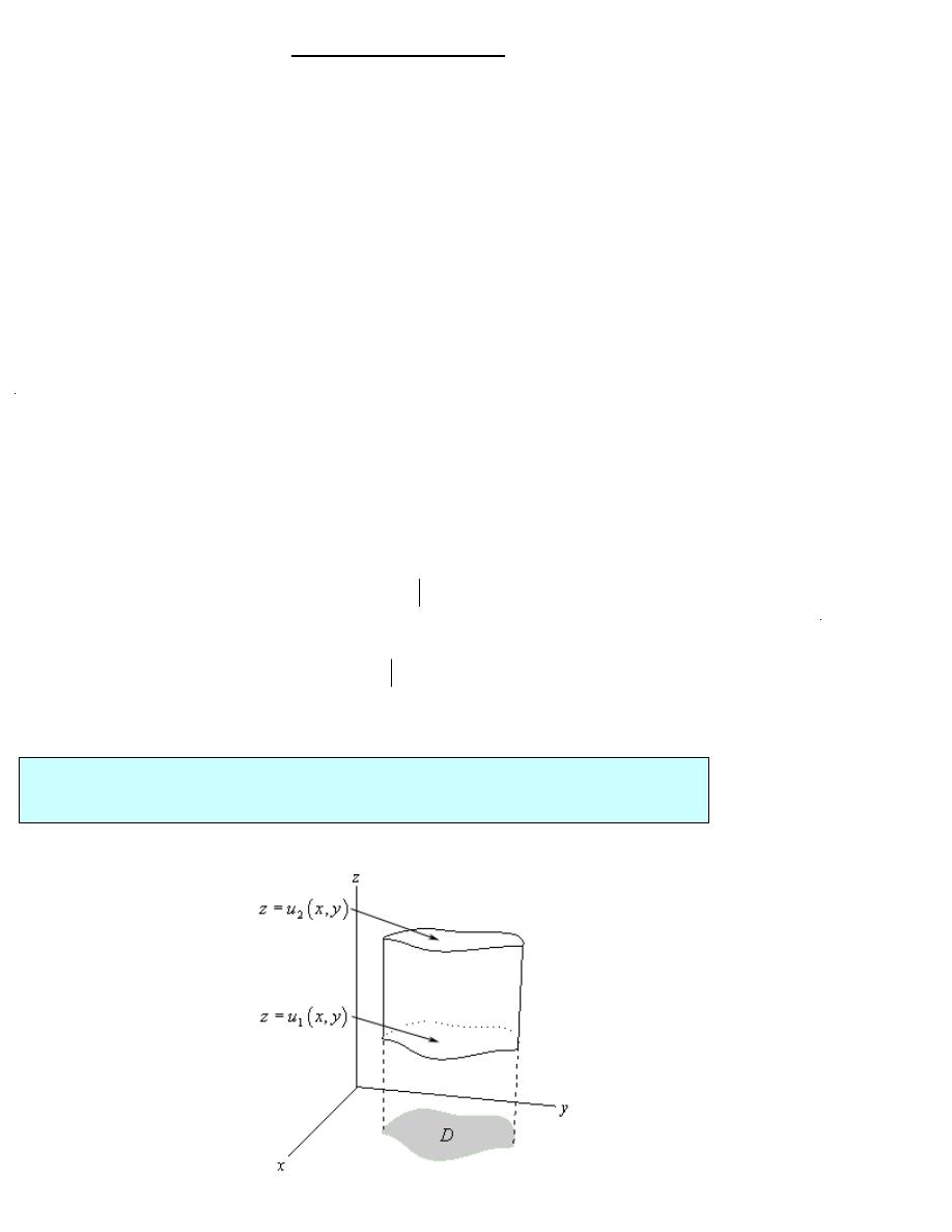
Let’s now move on the more general three-dimensional regions. We have three different
possibilities for a general region. Here is a sketch of the first possibility.
multiple Integral
21 of 39
<<2013-2014>>
Dr.Eng Muhammad.A.R.yass
Solution
In this case we will evaluate the triple integral as follows,
(
)
(
)
( )
( )
2
1
,
,
, ,
, ,
E
D
u x y
u x y
f x y z dV
f x y z dz dA
=
⌠⌠
⌡⌡
∫∫∫
∫
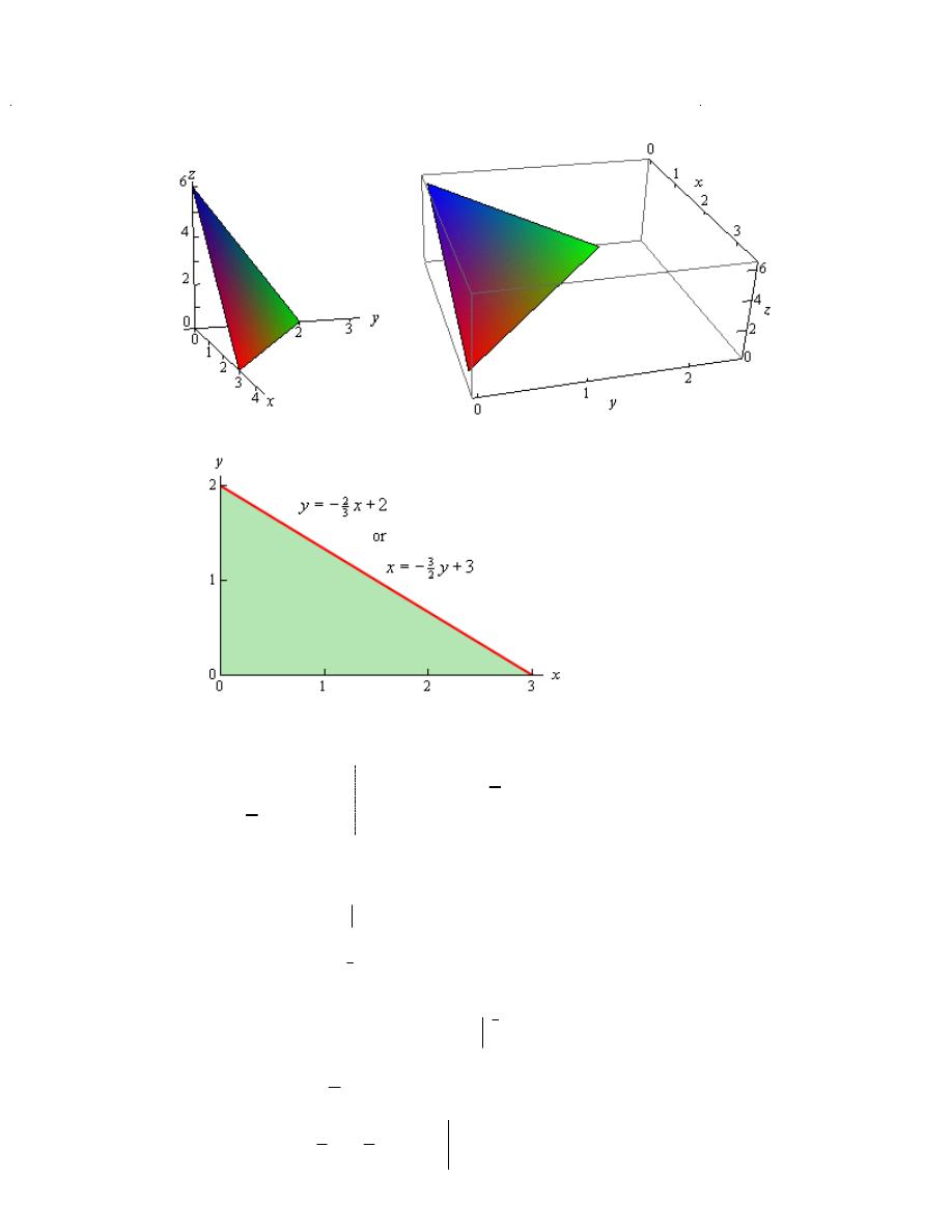
Example 2
Evaluate
2
E
x dV
∫∫∫
where E is the region under the plane
2
3
6
x
y
z
+
+ =
that lies
in the first octant.
. So D will be the triangle with vertices at
( )
0, 0
,
( )
3, 0
, and
( )
0, 2
. Here is a
sketch of D.
0
6 2
3
z
x
y
≤ ≤ −
−
We can integrate the double integral over D using either of the following two sets of inequalit
0
3
3
0
3
2
2
0
2
0
2
3
x
x
y
y
x
y
≤ ≤
≤ ≤ −
+
≤ ≤ −
+
≤ ≤
(
)
(
)
6 2
3
0
6 2
3
0
2
3
2
3
0
0
2
3
2
2
2
3
0
0
3
3
2
0
2
2
2
2
6 2
3
12
4
3
4
8
12
3
x
y
E
D
x
y
D
x
x
x dV
x dz dA
xz
dA
x
x
y dy dx
xy
x y
xy
dx
x
x
x dx
− −
− −
−
+
− +
=
=
=
−
−
=
−
−
=
−
+
⌠⌠
⌡⌡
⌠
⌡
⌠
⌡
⌠
⌡
∫∫∫
∫
∫∫
∫
3
4
3
2
0
1
8
6
3
3
9
x
x
x
=
−
+
=
multiple Integral
22 of 39
<<2013-2014>>
Dr.Eng Muhammad.A.R.yass
Solution
Here are the limits for each of the variables.
0
4
3
3
4
2
0
8
y
y
z
y
x
y
z
≤ ≤
≤ ≤
≤ ≤ − −
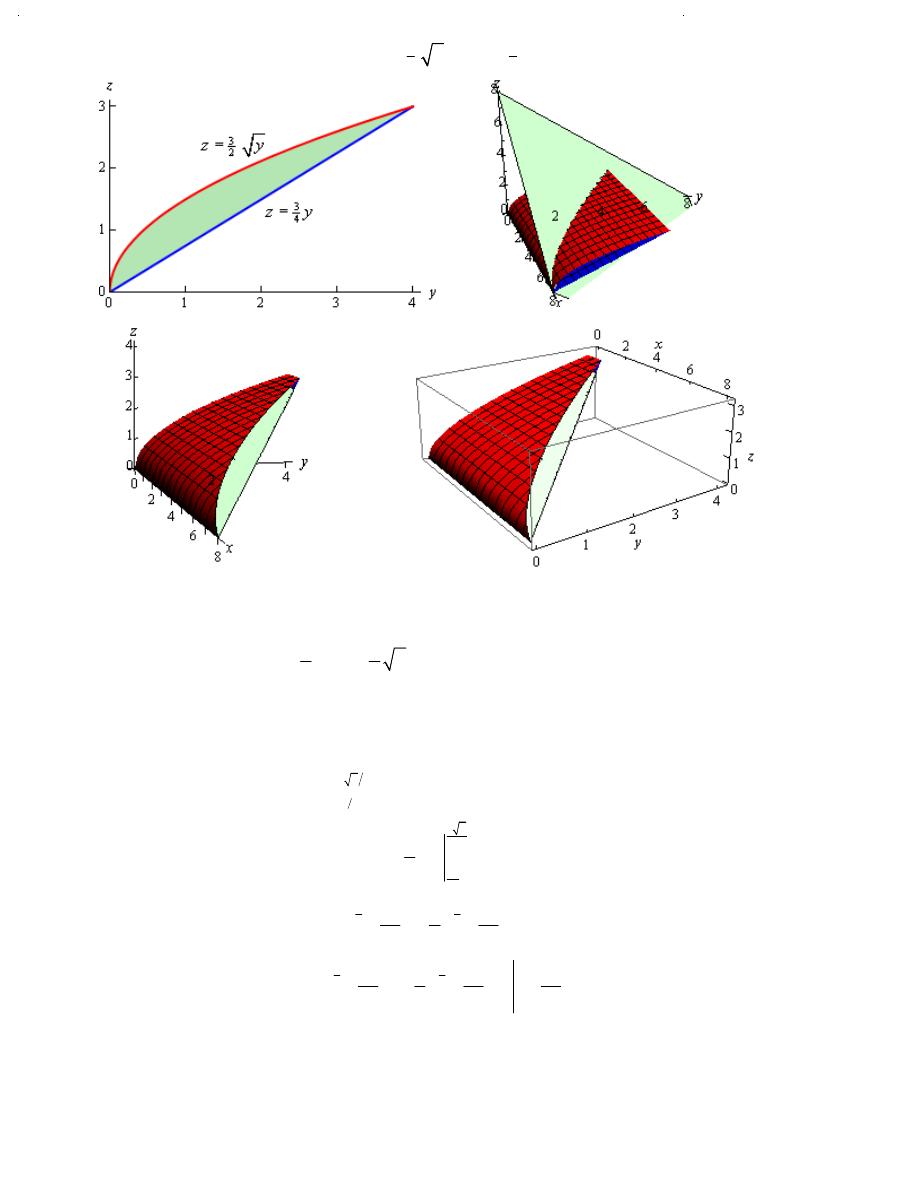
Example 3
Determine the volume of the region that lies behind the plane
8
x
y
z
+ + =
and in
front of the region in the yz-plane that is bounded by
3
2
z
y
=
and
3
4
z
y
=
.
8
0
4
3
2
3
4
0
4
3
2
2
3
4
0
8
1
8
2
y z
E
D
y
y
y
y
V
dV
dx dA
y
z dz dy
z
yz
z
dy
− −
=
=
=
− −
=
− −
⌠⌠
⌡⌡
⌠
⌡
⌠
⌡
∫∫∫
∫
∫
4
1
3
2
2
2
0
4
3
5
2
3
2
2
0
57
3
33
12
8
2
32
57
3
11
49
8
16
5
32
5
y
y
y
y dy
y
y
y
y
=
−
−
+
=
−
−
+
=
⌠
⌡
multiple Integral
23 of 39
<<2013-2014>>
Dr.Eng Muhammad.A.R.yass
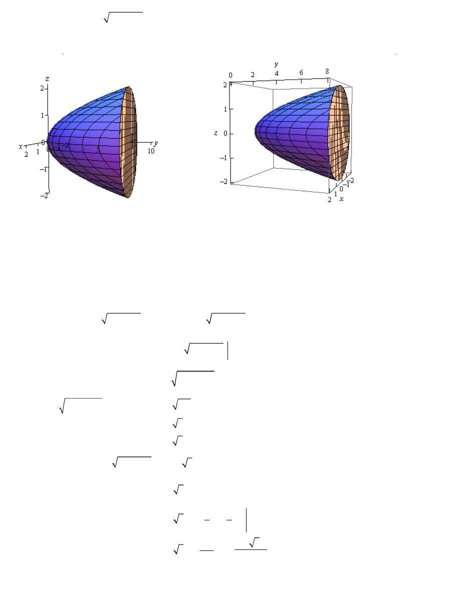
Example 4
Evaluate
2
2
3
3
E
x
z dV
+
∫∫∫
where E is the solid bounded by
2
2
2
2
y
x
z
=
+
and
the plane
8
y
=
.
Solution
Here is a sketch of the solid E.
2
2
2
2
2
2
8
4
x
z
x
z
+
=
⇒
+
=
cos
sin
x
r
z
r
θ
θ
=
=
2
2
2
x
z
r
+
=
2
2
2
2
8
0
2
0
2
x
z
y
r
θ
π
+
≤ ≤
≤ ≤
≤ ≤
(
)
(
) (
)
(
)
2
2
2
2
8
2
2
2
2
8
2
2
2
2
2
2
2
2
2
2
3
3
3
3
3
3
3
8
2
2
E
D
x
z
D
D
x
z
x
z dV
x
z dy dA
y
x
z
dA
x
z
x
z
dA
+
+
+
=
+
=
+
=
+
−
+
⌠⌠
⌡⌡
⌠⌠
⌡⌡
∫∫∫
∫
∫∫
(
) (
)
(
)
(
)
(
)
(
)
2
2
2
2
2
2
2
3
3
8
2
2
3
8 2
3
8 2
3 8
2
x
z
x
z
r
r
r
r
r
r
+
−
+
=
−
=
−
=
−
(
)
(
)
2
2
3
2
2
3
0
0
2
2
3
5
0
0
2
0
3
3
3 8
2
3
8
2
8
2
3
3
5
128
3
15
E
D
x
z dV
r
r
dA
r
r
r dr d
r
r
d
d
π
π
π
θ
θ
θ
+
=
−
=
−
=
−
=
⌠
⌡
⌠
⌡
⌠
⌡
∫∫∫
∫∫
∫
256 3
15
π
=
multiple Integral
24 of 39
<<2013-2014>>

Dr.Eng Muhammad.A.R.yass
Triple Integrals in Cylindrical Coordinates
The following are the conversion formulas for cylindrical coordinates.
cos
sin
x
r
y
r
z
z
θ
θ
=
=
=
dV
r dz dr d
θ
=
In terms of cylindrical coordinates a triple integral is,
(
)
(
)
(
)
(
)
( )
( )
2
2
1
1
cos , sin
cos , sin
, ,
cos , sin ,
E
h
u r
r
h
u r
r
f x y z dV
r f r
r
z dz dr d
β
θ
θ
θ
α
θ
θ
θ
θ
θ
θ
=
∫∫∫
∫ ∫ ∫
Example 1
Evaluate
E
y dV
∫∫∫
where E is the region that lies below the plane
2
z
x
= +
above
the xy-plane and between the cylinders
2
2
1
x
y
+
=
and
2
2
4
x
y
+
=
.
Solution
0
2
0
cos
2
z
x
z
r
θ
≤ ≤ +
⇒
≤ ≤
+
Remember that we are above the xy-plane and so we are above the plane
0
z
=
Next, the region D is the region between the two circles
2
2
1
x
y
+
=
and
2
2
4
x
y
+
=
in the xy-
plane and so the ranges for it are,
0
2
1
2
r
θ
π
≤ ≤
≤ ≤
(
)
(
)
( )
( )
2
2
0
1
0
2
2
2
0
1
2
2
3
2
0
1
2
2
4
3
1
0
cos
2
sin
sin
cos
2
1
sin 2
2
sin
2
1
2
sin 2
sin
8
3
E
r
y dV
r
r dz dr d
r
r
dr d
r
r
dr d
r
r
d
π
π
π
π
θ
θ
θ
θ
θ
θ
θ
θ
θ
θ
θ
θ
+
=
=
+
=
+
=
+
⌠
⌡
∫∫∫
∫ ∫ ∫
∫ ∫
∫ ∫
( )
( )
2
0
2
0
15
14
sin 2
sin
8
3
15
14
cos 2
cos
16
3
0
d
π
π
θ
θ θ
θ
θ
=
+
= −
−
=
⌠
⌡
Example 2
Convert
2
2
2
2
2
1
1
1
0
y
x
y
x
y
xyz dz dx dy
−
−
+
+
∫ ∫
∫
into an integral in cylindrical coordinates.
Solution
Here are the ranges of the variables from this iterated integral.
2
2
2
2
2
1
1
0
1
y
x
y
x
y
z
x
y
− ≤ ≤
≤ ≤
−
+
≤ ≤
+
2
1
x
y
=
−
from Integral Limits
multiple Integral
25 of 39
<<2013-2014>>

Dr.Eng Muhammad.A.R.yass
1
1
y
− ≤ ≤
2
2
0
1
r
π
π
θ
− ≤ ≤
≤ ≤
2
r
z
r
≤ ≤
(
)(
)
2
2
2
2
2
2
2
1
1
2
1
1
0
2
0
2
1
3
2
0
cos
sin
cos sin
r
r
y
x
y
x
y
r
r
xyz dz dx dy
r r
r
z dz dr d
zr
dz dr d
π
π
π
π
θ
θ
θ
θ
θ
θ
−
−
−
−
+
+
=
=
∫ ∫
∫
∫ ∫ ∫
∫ ∫ ∫
Limits of y
then
multiple Integral
26 of 39
<<2013-2014>>
Dr.Eng Muhammad.A.R.yass
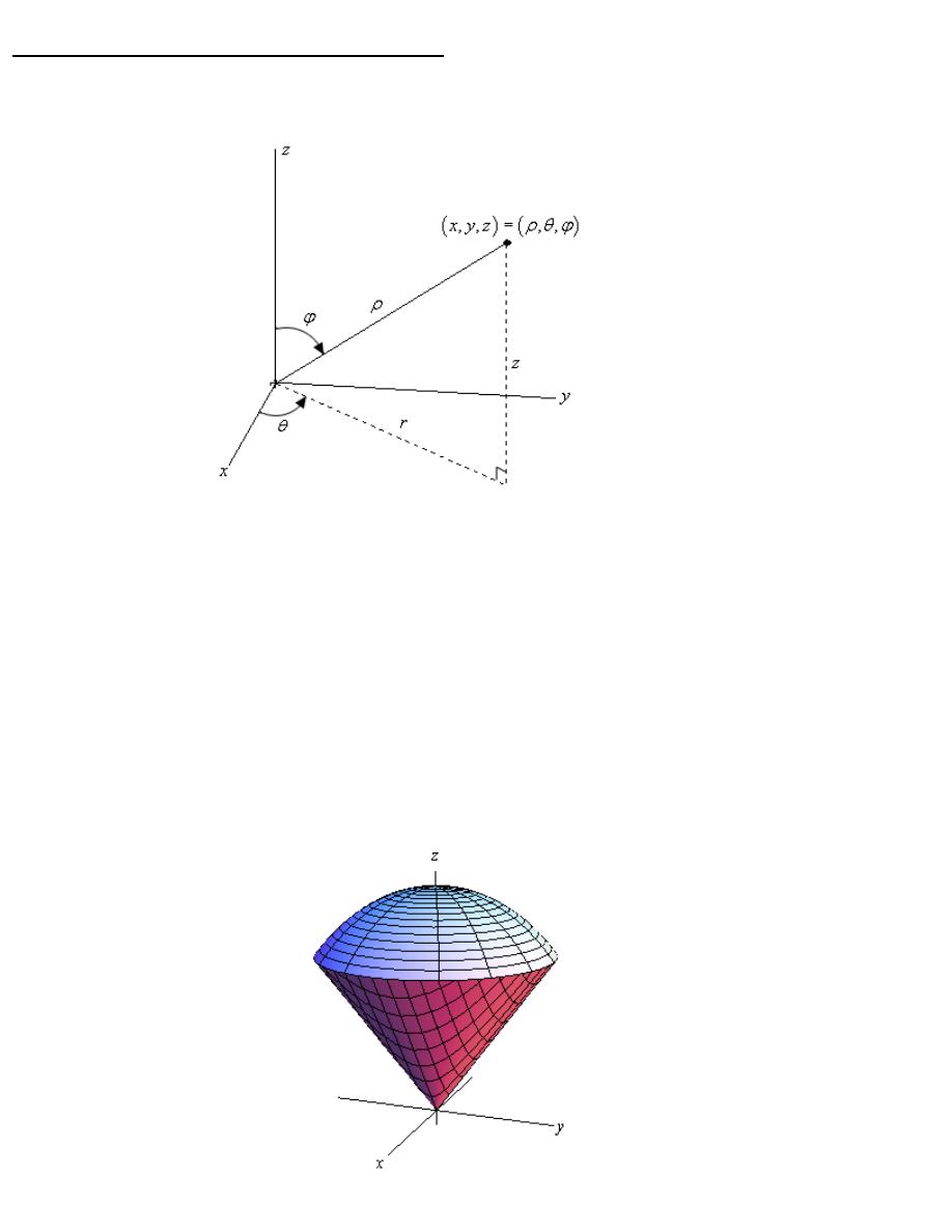
The following sketch shows the relationship between the Cartesian and spherical coordinate systems.
Here are the conversion formulas for spherical coordinates.
2
2
2
2
sin
cos
sin sin
cos
x
y
z
x
y
z
ρ
ϕ
θ
ρ
ϕ
θ
ρ
ϕ
ρ
=
=
=
+
+
=
We also have the following restrictions on the coordinates.
0
0
ρ
ϕ π
≥
≤ ≤
For our integrals we are going to restrict E down to a spherical wedge. This will mean that we
are going to take ranges for the variables as follows,
a
b
ρ
α θ β
δ ϕ γ
≤ ≤
≤ ≤
≤ ≤
Here is a quick sketch of a spherical wedge in which the lower limit for both
ρ
and
ϕ
are zero
for reference purposes. Most of the wedges we’ll be working with will fit into this pattern.
Triple Integrals in Spherical coordinates
multiple Integral
27 of 39
<<2013-2014>>
Dr.Eng Muhammad.A.R.yass
2
sin
dV
d d d
ρ
ϕ ρ θ ϕ
=
Therefore the integral will become,
(
)
(
)
2
, ,
sin
sin cos , sin sin , cos
E
b
a
f x y z dV
f
d d d
β γ
α
δ
ρ
ϕ
ρ
ϕ
θ ρ
ϕ
θ ρ
ϕ ρ θ ϕ
=
∫∫∫
∫ ∫ ∫
The integral is then,
also
Example 1
Evaluate
16
E
z dV
∫∫∫
where E is the upper half of the sphere
2
2
2
1
x
y
z
+
+
=
.
Solution
Since we are taking the upper half of the sphere the limits for the variables are,
0
1
0
2
0
2
ρ
θ
π
π
ϕ
≤ ≤
≤ ≤
≤ ≤
(
)
( )
( )
( )
2
2
3
2
2
2
0
0
0
2
1
0
0
0
2
0
0
0
16
sin
16 cos
8
sin 2
2sin 2
4 sin 2
E
z dV
d
d d
d
d d
d d
d
π
π
π
π
π
π
ρ
ϕ
ρ
ϕ ρ θ ϕ
ρ
ϕ ρ θ ϕ
ϕ θ ϕ
π
ϕ ϕ
=
=
=
=
∫∫∫
∫ ∫ ∫
∫ ∫ ∫
∫ ∫
∫
2
1
π
( )
2
0
2 cos 2
4
π
π
ϕ
π
= −
=
Example 2
Convert
2
2
2
2
2
3
9
2
2
2
0
0
18
y
x
y
x
y
x
y
z dz dx dy
−
−
−
+
+
+
∫ ∫
∫
into spherical coordinates.
Solution
Let’s first write down the limits for the variables.
2
2
2
2
2
0
3
0
9
18
y
x
y
x
y
z
x
y
≤ ≤
≤ ≤
−
+
≤ ≤
− −
(since this is the angle around the z-axis).
0
2
π
θ
≤ ≤
The lower bound,
2
2
z
x
y
=
+
,
.
2
2
18
z
x
y
=
− −
The upper bound,
upper half of the sphere,
2
2
2
18
x
y
z
+
+
=
and so from this we now have the following range for
ρ
0
18
3 2
ρ
≤ ≤
=
Now all that we need is the range for
ϕ
. There are two ways to get this. One is from where the
cone and the sphere intersect. Plugging in the equation for the cone into the sphere gives,
(
)
2
2
2
2
2
2
2
18
18
9
3
x
y
z
z
z
z
z
+
+
=
+
=
=
=
multiple Integral
28 of 39
<<2013-2014>>

Dr.Eng Muhammad.A.R.yass
we know that
3 2
ρ
=
since we are intersecting on the sphere. This gives,
cos
3
3 2 cos
3
1
2
cos
2
4
2
ρ
ϕ
ϕ
π
ϕ
ϕ
=
=
=
=
⇒
=
The other way to get this range is from the cone by itself. By first converting the equation into
cylindrical coordinates and then into spherical coordinates we get the following,
cos
sin
1
tan
4
z
r
ρ
ϕ ρ
ϕ
π
ϕ
ϕ
=
=
=
⇒
=
So, recalling that
2
2
2
2
x
y
z
ρ
=
+
+
, the integral is then,
2
2
2
2
2
3
9
4
2
3 2
2
2
2
4
0
0
0
0
0
18
sin
y
x
y
x
y
x
y
z dz dx dy
d d d
π
π
ρ
ϕ ρ θ ϕ
−
−
−
+
+
+
=
∫ ∫
∫
∫ ∫ ∫
So, it looks like we have the following range,
0
4
π
ϕ
≤ ≤
multiple Integral
29 of 39
<<2013-2014>>
Dr.Eng Muhammad.A.R.yass
substitution rule that told us that,
( )
(
)
( )
( )
( )
where
b
d
a
c
f g x
g x dx
f u du
u
g x
′
=
=
∫
∫
Change of Variables
First we need a little notation out of the way. We call the equations that define the change of
variables a transformation. Also we will typically start out with a region, R, in xy-coordinates
and transform it into a region in uv-coordinates.
Example 1
Determine the new region that we get by applying the given transformation to the
region R.
(a) R is the ellipse
2
2
1
36
y
x
+
=
and the transformation is
2
u
x
=
,
3
y
v
=
.
(b) R is the region bounded by
4
y
x
= − +
,
1
y
x
= +
, and
4
3
3
x
y
= −
and the
transformation is
(
)
1
2
x
u
v
=
+
,
(
)
1
2
y
u
v
=
−
.
Solution
(a) R is the ellipse
2
2
1
36
y
x
+
=
and the transformation is
2
u
x
=
,
3
y
v
=
.
There really isn’t too much to do with this one other than to plug the transformation into the
equation for the ellipse and see what we get.
( )
2
2
2
2
2
2
3
1
2
36
9
1
4
36
4
v
u
u
v
u
v
+
=
+
=
+ =
So, we started out with an ellipse and after the transformation we had a disk of radius 2.
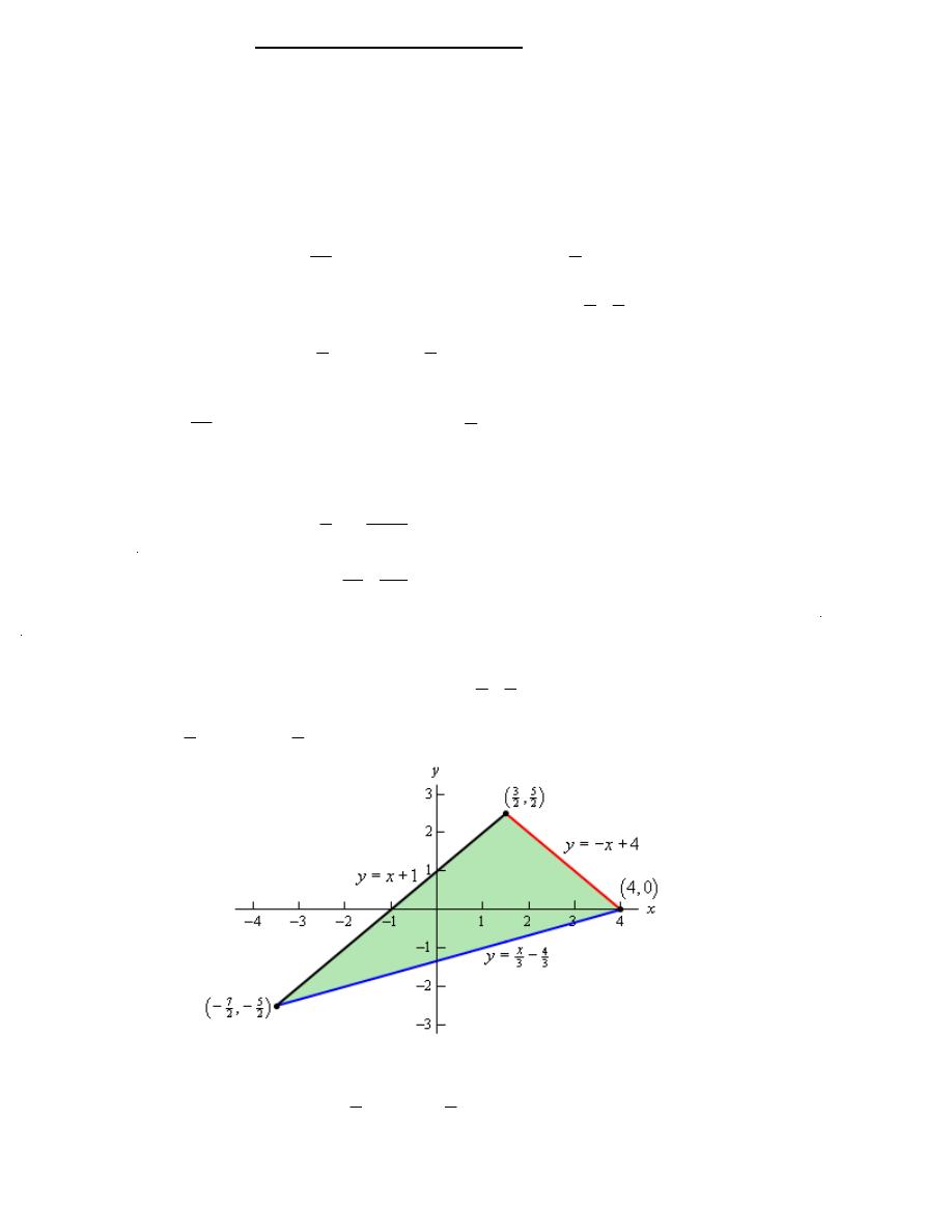
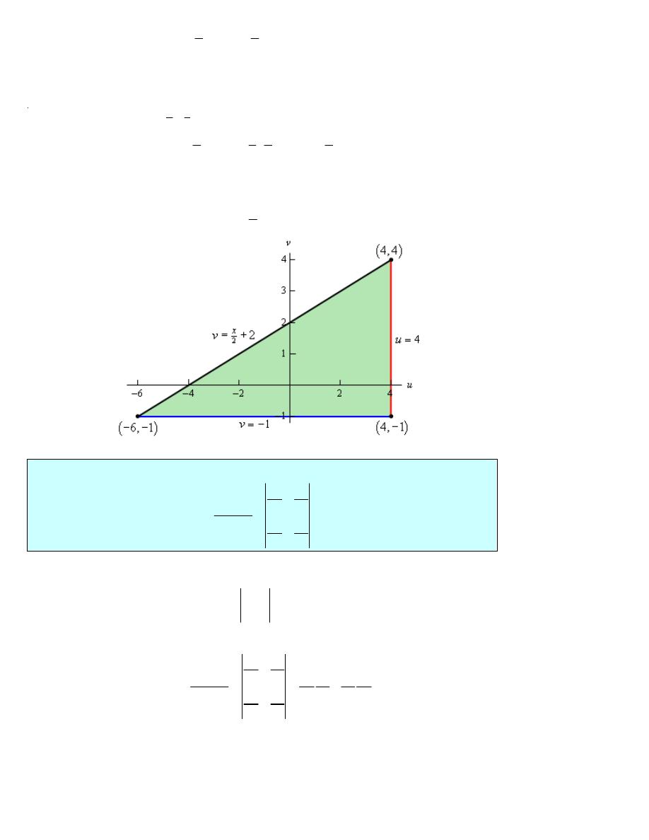
(b) R is the region bounded by
4
y
x
= − +
,
1
y
x
= +
, and
4
3
3
x
y
= −
and the
transformation is
(
)
1
2
x
u
v
=
+
,
(
)
1
2
y
u
v
=
−
.
Let’s do
4
y
x
= − +
first. Plugging in the transformation gives
,
(
)
(
)
1
1
4
2
2
8
2
8
4
u v
u
v
u
v
u
v
u
u
− = −
+ +
− = − − +
=
=
multiple Integral
30 of 39
<<2013-2014>>
Dr.Eng Muhammad.A.R.yass
Now let’s take a look at
1
y
x
= +
,
(
)
(
)
1
1
1
2
2
2
2
2
1
u
v
u
v
u
v
u
v
v
v
− =
+ +
− = + =
− =
= −
Finally, let’s transform
4
3
3
x
y
= −
.
(
)
(
)
1
1 1
4
2
3 2
3
3
3
8
4
2
8
2
2
u
v
u
v
u
v
u
v
v
u
u
v
− =
+
−
− = + −
=
+
= +
Definition
The Jacobian of the transformation
( )
,
x
g u v
=
,
( )
,
y
h u v
=
is
( )
( )
,
,
x
x
x y
u
v
y
y
u v
u
v
∂
∂
∂
∂
∂
=
∂
∂
∂
∂
∂
The Jacobian is defined as a determinant of a 2x2 matrix, if you are unfamiliar with this that is
okay. Here is how to compute the determinant.
a
b
ad
bc
c
d
=
−
Therefore, another formula for the determinant is,
( )
( )
,
,
x
x
x y
x y
x y
u
v
y
y
u v
u v
v u
u
v
∂
∂
∂
∂ ∂
∂ ∂
∂
∂
=
=
−
∂
∂
∂
∂ ∂
∂ ∂
∂
∂
multiple Integral
31 of 39
<<2013-2014>>
Dr.Eng Muhammad.A.R.yass
Change of Variables for a Double Integral
Suppose that we want to integrate
( )
,
f x y
over the region R. Under the transformation
( )
,
x
g u v
=
,
( )
,
y
h u v
=
the region becomes S and the integral becomes,
( )
( ) ( )
(
)
( )
( )
,
,
,
,
,
,
D
S
x y
f x y dA
f g u v h u v
du dv
u v
∂
=
∂
⌠⌠
⌡⌡
∫∫
If we look just at the differentials in the above formula we can also say that
( )
( )
,
,
x y
dA
du dv
u v
∂
=
∂
Example 2
Show that when changing to polar coordinates we have
dA
r dr d
θ
=
Solution
The transformation here is the standard conversion formulas,
cos
sin
x
r
y
r
θ
θ
=
=
The Jacobian for this transformation is,
( )
( )
(
)
(
)
2
2
2
2
,
,
cos
sin
sin
cos
cos
sin
cos
sin
x
x
x y
r
y
y
r
r
r
r
r
r
r
r
θ
θ
θ
θ
θ
θ
θ
θ
θ
θ
θ
∂
∂
∂
∂
∂
=
∂
∂
∂
∂
∂
−
=
=
− −
=
+
=
We then get,
( )
( )
,
,
x y
dA
dr d
r dr d
r dr d
r
θ
θ
θ
θ
∂
=
=
=
∂
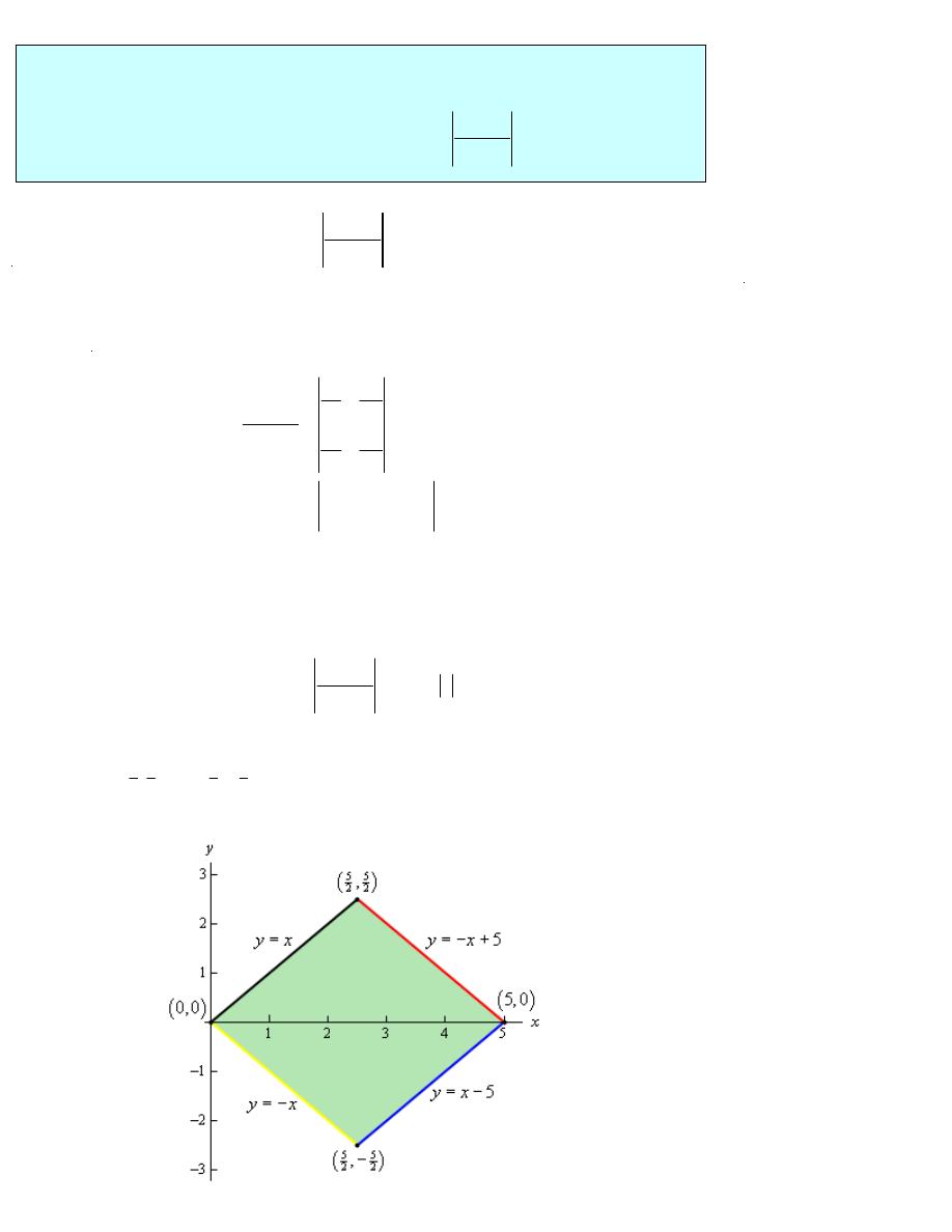
Example 3
Evaluate
R
x
y dA
+
∫∫
where R is the trapezoidal region with vertices given by
( )
0, 0
,
( )
5, 0
,
( )
5
5
2
2
,
and
(
)
5
5
2
2
,
−
using the transformation
2
3
x
u
v
=
+
and
2
3
y
u
v
=
−
.
Solution
First, let’s sketch the re ion R and determine e uations for each of the sides.
multiple Integral
32 of 39
<<2013-2014>>

Dr.Eng Muhammad.A.R.yass
Next we’ll transform
5
y
x
= − +
.
(
)
2
3
2
3
5
4
5
5
4
u
v
u
v
u
u
− = −
+
+
=
=
Finally, let’s transform
5
y
x
= −
.
2
3
2
3
5
6
5
5
6
u
v
u
v
v
v
− =
+ −
− = −
=
The region S is then a rectangle whose sides are given by
0
u
=
,
0
v
=
,
5
4
u
=
and
5
6
v
=
and s
o
the ranges of u and v are,
5
5
0
0
4
6
u
v
≤ ≤
≤ ≤
Next, we need the Jacobian.
( )
( )
2
3
,
6 6
12
2
3
,
x y
u v
∂
=
= − − = −
−
∂
Let’s use the transformation and see what we get. We’ll do this by plugging the transformation
into each of the equations above.
Let’s start the process off with
y
x
=
.
2
3
2
3
6
0
0
u
v
u
v
v
v
− =
+
=
=
Transforming
y
x
= −
is similar.
(
)
2
3
2
3
4
0
0
u
v
u
v
u
u
− = −
+
=
=
(
) (
)
5
5
6
4
0
0
5
5
6
4
0
0
5
5
6
2 4
0
0
5
6
0
2
3
2
3
12
48
24
75
2
R
x
y dA
u
v
u
v
du dv
u du dv
u
dv
dv
+
=
+
+
−
−
=
=
=
⌠
⌡
⌠
⌡
⌠
⌡
⌠
⌡
∫∫
∫
∫
The integral is then,
5
6
0
75
2
125
4
v
=
=
multiple Integral
33 of 39
<<2013-2014>>
Dr.Eng Muhammad.A.R.yass
Example 4
Evaluate
2
2
R
x
xy
y dA
− +
∫∫
where R is the ellipse given by
2
2
2
x
xy
y
−
+
=
and
using the transformation
2
3
2
x
u
v
=
−
,
2
3
2
y
u
v
=
+
.
Solution
The first thing to do is to plug the transformation into the equation for the ellipse to see what the
region transforms into.
2
2
2
2
2
2
2
2
2
2
2
2
2
2
2
2
2
2
2
2
2
3
3
3
3
4
2
2
4
2
2
2
2
3
3
3
3
3
2
2
x
xy
y
u
v
u
v
u
v
u
v
u
uv
v
u
v
u
uv
v
u
v
=
−
+
=
−
−
−
+
+
+
=
−
+
−
−
+
+
+
=
+
( )
( )
2
2
,
2
2
4
3
,
3
3
3
2
2
3
x y
u v
−
∂
=
=
+
=
∂
The integral is then,
(
)
2
2
2
2
4
2
3
R
S
x
xy
y dA
u
v
du dv
− +
=
+
⌠⌠
⌡⌡
∫∫
Do not make the mistake of substituting
.
2
2
2
x
x
−
+
=
or
2
2
1
u
v
+ =
in for the integrands.
the integral out will convert to polar coordinates.
(
)
( )
2
2
2
2
2
1
2
0
0
2
1
4
0
0
2
0
4
2
3
8
3
8
1
4
3
8
1
4
3
4
3
R
S
x
xy
y dA
u
v
du dv
r
r dr d
r
d
d
π
π
π
θ
θ
θ
π
− +
=
+
=
=
=
=
⌠⌠
⌡⌡
⌠
⌡
⌠
⌡
⌠
⌡
∫∫
∫
multiple Integral
34 of 39
<<2013-2014>>
Dr.Eng Muhammad.A.R.yass
Let’s now briefly look at triple integrals. In this case we will again start with a region R and use
the transformation
(
)
, ,
x
g u v w
=
,
(
)
, ,
y
h u v w
=
, and
(
)
, ,
z
k u v w
=
to transform the region
into the new region S. To do the integral we will need a Jacobian, just as we did with double
integrals. Here is the definition of the Jacobian for this kind of transformation.
(
)
(
)
, ,
, ,
x
x
x
u
v
w
x y z
y
y
y
u v w
u
v
w
z
z
z
u
v
w
∂
∂
∂
∂
∂
∂
∂
∂
∂
∂
=
∂
∂
∂
∂
∂
∂
∂
∂
∂
∂
The integral under this transformation is,
(
)
(
) (
) (
)
(
)
(
)
(
)
, ,
, ,
, ,
,
, ,
,
, ,
, ,
R
S
x y z
f x y z dV
f g u v w h u v w k u v w
du dv dw
u v w
∂
=
∂
⌠⌠⌠
⌡⌡⌡
∫∫∫
As with double integrals we can look at just the differentials and note that we must have
(
)
(
)
, ,
, ,
x y z
dV
du dv dw
u v w
∂
=
∂
Example 5
Verify that
2
sin
dV
d d d
ρ
ϕ ρ θ ϕ
=
when using spherical coordinates.
Solution
Here the transformation is just the standard conversion formulas.
sin
cos
sin sin
cos
x
y
z
ρ
ϕ
θ
ρ
ϕ
θ
ρ
ϕ
=
=
=
The Jacobian is,
(
)
(
)
sin cos
sin sin
cos cos
, ,
sin sin
sin cos
cos sin
, ,
cos
0
sin
z y z
ϕ
θ
ρ
ϕ
θ ρ
ϕ
θ
ϕ
θ
ρ
ϕ
θ
ρ
ϕ
θ
ρ θ ϕ
ϕ
ρ
ϕ
−
∂
=
∂
−
(
)
(
)
2
3
2
2
2
2
2
3
2
2
2
2
2
3
2
2
2
2
2
2
2
3
2
sin
cos
sin
cos
sin
0
sin
sin
0
sin
cos
cos
sin
cos
sin
sin cos
sin
cos
sin
sin
ρ
ϕ
θ ρ
ϕ
ϕ
θ
ρ
ϕ
θ
ρ
ϕ
ϕ
θ
ρ
ϕ
θ
θ
ρ
ϕ
ϕ
θ
θ
ρ
ϕ ρ
= −
−
+
−
− −
= −
+
−
+
= −
−
(
)
2
2
2
2
2
cos
sin
sin
cos
sin
ϕ
ϕ
ρ
ϕ
ϕ
ϕ
ρ
ϕ
= −
+
= −
Finally, dV becomes,
2
2
sin
sin
dV
d d d
d d d
ρ
ϕ ρ θ ϕ ρ
ϕ ρ θ ϕ
= −
=
Recall that we restricted
ϕ
to the range
0
ϕ π
≤ ≤
for spherical coordinates and so we know that
sin
0
ϕ
≥
and so we don’t need the absolute value bars on the sine.
multiple Integral
35 of 39
<<2013-2014>>
Dr.Eng Muhammad.A.R.yass
Here we want to find the surface area of the surface given by
( )
,
z
f x y
=
where
( )
,
x y
is a
point from the region D in the xy-plane. In this case the surface area is given by,
[ ]
2
2
1
x
y
D
S
f
f
dA
=
+
+
⌠⌠
⌡⌡
Surface Area
Example 1
Find the surface area of the part of the plane
3
2
6
x
y
z
+
+ =
that lies in the first
octant.
Solution
( )
,
z
f x y
=
6 3
2
3
2
x
y
z
x
y
f
f
= − −
= −
= −
then
so
and
The limits defining D are,
3
0
2
0
3
2
x
y
x
≤ ≤
≤ ≤ −
+
The surface area is then,
[ ] [ ]
2
2
3
2
3
2
0
0
2
0
3
2
1
14
3
14
3
2
D
x
S
dA
dy dx
x
dx
−
+
=
−
+ −
+
=
=
−
+
∫∫
∫ ∫
∫
2
2
0
3
14
3
4
3 14
x
x
=
−
+
=
multiple Integral
36 of 39
<<2013-2014>>
Dr.Eng Muhammad.A.R.yass
Example 2
Determine the surface area of the part of
z
xy
=
that lies in the cylinder given by
2
2
1
x
y
+
=
.
Here are the partial derivatives,
x
y
f
y
f
x
=
=
Solution
The integral for the surface area is,
2
2
1
D
S
x
y
dA
=
+
+
∫∫
Given that D is a disk it makes sense to do this integral in polar coordinates.
(
)
2
2
2
1
2
0
0
2
1
3
2
2
0
0
2
3
2
0
1
1
1 2
1
2 3
1
2
1
3
D
S
x
y
dA
r
r dr d
r
d
d
π
π
π
θ
θ
θ
=
+
+
=
+
=
+
=
−
⌠
⌡
⌠
⌡
∫∫
∫ ∫
3
2
2
2
1
3
π
=
−
multiple Integral
37 of 39
<<2013-2014>>

Dr.Eng Muhammad.A.R.yass
We’ll first look at the area of a region. The area of the region D is given by,
Area of
D
D
dA
=
∫∫
Now let’s give the two volume formulas. First the volume of the region E is given by,
Volume of
E
E
dV
=
∫∫∫
Area and Volume Revisited
Finally, if the region E can be defined as the region under the function
( )
,
z
f x y
=
and above
the region D in xy-plane then,
( )
Volume of
,
D
E
f x y dA
=
∫∫
Note as well that there are similar formulas for the other planes. For instance, the volume of the
region behind the function
( )
,
y
f x z
=
and in front of the region D in the xz-plane is given by,
( )
Volume of
,
D
E
f x z dA
=
∫∫
Likewise, the the volume of the region behind the function
( )
,
x
f y z
=
and in front of the
region D in the yz-plane is given by,
( )
Volume of
,
D
E
f y z dA
=
∫∫
multiple Integral
38 of 39
<<2013-2014>>
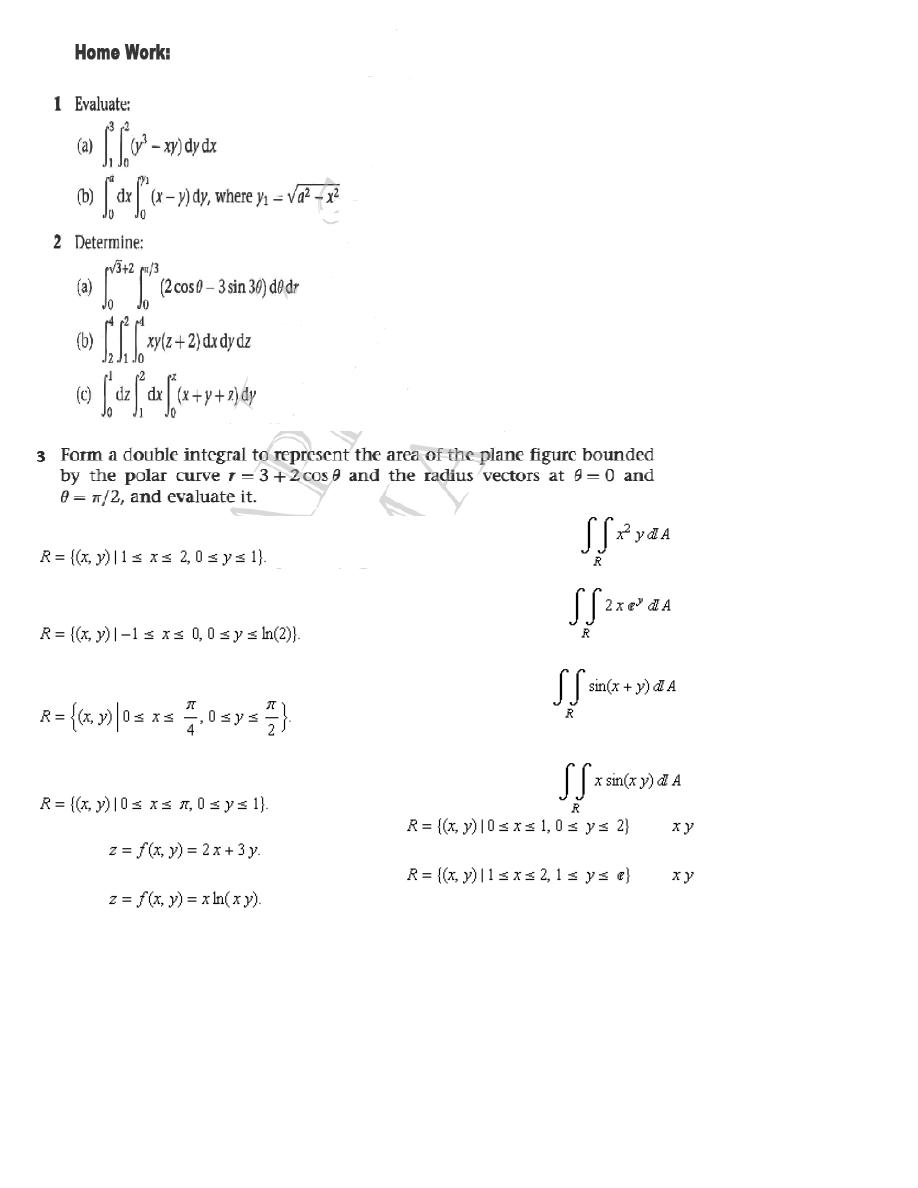
multiple Integral
39 of 39
<<2013-2014>>
(4) Use iterated integration to compute the double integral of the rectangular region
over the rectangle
(5) Use iterated integration to compute the double integral of the rectangular region
over the rectangle
(6)
Use iterated integration to compute the double integral of the rectangular region
over the rectangle
(7) Use iterated integration to compute the double integral of the rectangular region
over the rectangle
(8) Find the volume of the solid bounded below by the rectangle
in the
-plane and above
the graph of
(9) Find the volume of the solid bounded below by the rectangle
in the
-plane and above
the graph of
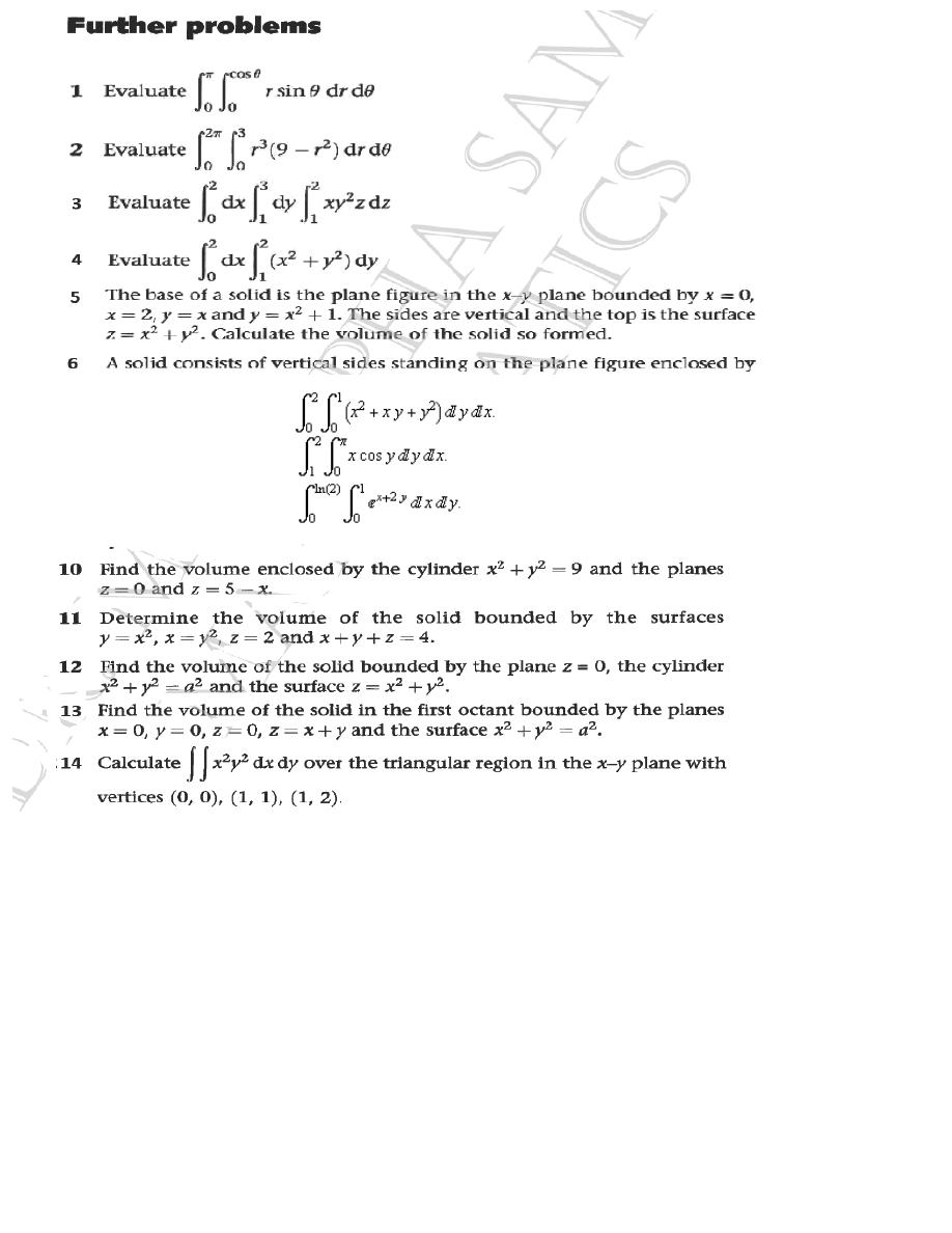
<<2012-2013>>
multiple Integral
39a of 39
<<2012-2013>>
Evaluate the iterated integral
Evaluate the iterated integral
Evaluate the iterated integral
7
8
9