
2
nd
P
A
d
Clas
Part
Adva
s
Uni
Electro
tial
anc
iversity of
omechani
Energy
Dif
ced
f Technolo
cal Depar
Branch
ffer
Ma
ogy
tment
rent
athe
tiat
ema
tion
atic
1
st
Le
n
cs
cture
Dr.Eng Muhammad.A.R.yass
Partial Derivatives
Recall that given a function of one variable,
( )
f x
, the derivative,
( )
f x
¢
, represents the rate of
change of the function as x changes. This is an important interpretation of derivatives and we are
not going to want to lose it with functions of more than one variable. The problem with functions
of more than one variable is that there is more than one variable. In other words, what do we do
if we only want one of the variables to change, or if we want more than one of them to change?
In fact, if we’re going to allow more than one of the variables to change there are then going to be
an infinite amount of ways for them to change. For instance, one variable could be changing
faster than the other variable(s) in the function. Notice as well that it will be completely possible
for the function to be changing differently depending on how we allow one or more of the
variables to change.
Let’s start with the function
( )
2 3
,
2
f x y
x y
=
the partial derivatives from above will
more commonly be written as,
( )
( )
3
2
2
,
4
and
,
6
x
y
f x y
xy
f x y
x y
=
=
Since we can think of the two partial derivatives above as derivatives of single variable functions
it shouldn’t be too surprising that the definition of each is very similar to the definition of the
derivative for single variable functions. Here are the formal definitions of the two partial
derivatives we looked at above.
( )
(
)
( )
( )
(
)
( )
0
0
,
,
,
,
,
lim
,
lim
x
y
h
h
f x h y
f x y
f x y h
f x y
f x y
f x y
h
h
®
®
+
-
+
-
=
=
Now let’s take a quick look at some of the possible alternate notations for partial derivatives.
Given the function
( )
,
z
f x y
=
the following are all equivalent notations,
( )
( )
(
)
( )
( )
(
)
,
,
,
,
x
x
x
x
y
y
y
y
f
z
f x y
f
f x y
z
D f
x
x
x
f
z
f x y
f
f x y
z
D f
y
y
y
=
=
=
=
=
=
=
=
=
=
=
=
For the fractional notation for the partial derivative notice the difference between the partial
derivative and the ordinary derivative from single variable calculus.
( )
( )
( )
( )
( )
,
,
&
,
x
y
df
f x
f x
dx
f
f
f x y
f x y
f x y
x
y
¢
Þ
=
Þ
=
=
Example 1
Find all of the first order partial derivatives for the following functions.
(a)
( )
4
,
6
10
f x y
x
y
=
+
-
(b)
( )
2
2 3
10
43
7 tan 4
w x y
y z
x
y
=
-
+
-
(c)
( )
( )
7
7
2
4
3
9
,
ln
h s t
t
s
s
t
=
+ -
(d)
( )
2
3
5
4
,
cos
x y
y
f x y
x
-
æ ö
=
ç ÷
è ø
e
1
Dr.Eng Muhammad.A.R.yass
Solution
a)
( )
4
,
6
10
f x y
x
y
=
+
-
( )
3
,
4
x
f x y
x
=
( )
3
,
y
f x y
y
=
(b)
( )
2
2 3
10
43
7 tan 4
w x y
y z
x
y
=
-
+
-
.
2
43
w
xy
x
=
+
( )
2
3
2
20
28sec 4
w
x
yz
y
y
=
-
-
2 2
30
w
y z
z
= -
t
(c)
( )
( )
7
7
2
4
3
9
,
ln
h s t
t
s
s
=
+ -
( )
( )
4
7
2
3
7
,
ln
9
h s t
t
s
t
s
-
=
+
-
=
( )
( )
( )
3
3
7
7
7
7
2
6
2
4
2
4
2
4
,
7
7
,
7 ln
27
s
t
h
s
t
h s t
t
s
s
s
s
s
h
h s t
t
s
t
t
-
-
-
æ
ö
=
=
-
=
-
ç
÷
è
ø
=
=
-
Remember how to differentiate natural logarithms.
( )
(
)
( )
( )
ln
g x
d
g x
dx
g x
¢
=
(d)
( )
2
3
5
4
,
cos
x y
y
f x y
x
-
æ ö
=
ç ÷
è ø
e
.
( )
(
)
2
3
2
3
2
3
2
3
2
2
5
5
5
5
4
4
4
,
sin
cos
2
4
4
4
sin
2 cos
x
x y
y
x y
y
x y
y
x y
y
f x y
xy
x
x
x
xy
x
x
x
-
-
-
-
æ öæ
ö
æ ö
= -
-
+
ç ÷ç
÷
ç ÷
è øè
ø
è ø
æ ö
æ ö
=
+
ç ÷
ç ÷
è ø
è ø
e
e
e
e
Also, don’t forget how to differentiate exponential functions,
( )
( )
( )
( )
f x
f x
d
f x
dx
¢
=
e
e
.
.
( )
(
)
2
3
2
2
5
4
,
15
cos
y
x y
y
f x y
x
y
x
-
æ ö
=
-
ç ÷
è ø
e
Example 2
Find all of the first order partial derivatives for the following functions.
(a)
2
9
5
u
z
u
v
=
+
(b)
(
)
( )
2
sin
, ,
x
y
g x y z
z
=
(c)
(
)
2
2
ln 5
3
z
x
x
y
=
+
-
Solution
(a)
2
9
5
u
z
u
v
=
+
.
(
)
( )
(
)
(
)
( )
(
)
( )
(
)
(
)
2
2
2
2
2
2
2
2
2
2
2
9
5
9 2
9
45
5
5
0
5
9 5
45
5
5
u
v
u
v
u u
u
v
z
u
v
u
v
u
v
u
u
z
u
v
u
v
+
-
-
+
=
=
+
+
+
-
-
=
=
+
+
2
Dr.Eng Muhammad.A.R.yass
(b)
(
)
( )
2
sin
, ,
x
y
g x y z
=
(
)
( )
(
)
( )
2
2
sin
cos
, ,
, ,
x
y
y
x
y
g x y z
g x y z
z
z
=
=
(
)
( )
(
)
( )
( )
2
3
3
, ,
sin
2 sin
, ,
2 sin
z
g x y z
x
y z
x
y
g x y z
x
y z
z
-
-
=
= -
= -
z
x
y
(c)
(
)
2
2
ln 5
3
z
x
x
y
=
+
-
(
)
(
)
(
)
(
)
(
)
(
)
(
)
(
)
(
)
1
2
2
2
2
2
1
2
2
2
2
1
2
2
2
2
1
ln 5
3
ln 5
3
2
1
5
ln 5
3
2
2
5
3
5
ln 5
3
2 5
3
x
z
x
x
y
x
x
y
x
x
x
y
x
x
y
x
x
x
y
x
y
-
-
-
=
+
-
+
-
æ
ö
=
+
-
+
ç
÷
-
è
ø
æ
ö
ç
÷
=
+
+
-
ç
÷
-
è
ø
(
)
(
)
(
)
(
)
(
)
(
)
(
)
(
)
1
2
2
2
2
2
1
2
2
2
2
1
2
2
2
2
1
ln 5
3
ln 5
3
2
1
6
ln 5
3
2
5
3
3
ln 5
3
5
3
y
z
x
x
y
x
x
y
y
y
x
x
y
x
y
y
x
x
y
-
-
-
=
+
-
+
-
æ
ö
-
=
+
-
ç
÷
-
è
ø
= -
+
-
-
Example 3
Find
dy
dx
for
4
7
3
5
y
x
x
+
=
.
Solution
The first step is to differentiate both sides with respect to x.
3
6
12
7
5
dy
y
x
dx
+
=
6
3
5 7
12
dy
x
dx
y
-
=
Example 4
Find
z
x
and
z
y
for each of the following functions.
(a)
3 2
5
2
3
5
x z
xy z x
y
-
=
+
(b)
(
)
( )
2
sin 2
5
1
cos 6
x
y
z
y
zx
-
= +
Solution
(a)
3 2
5
2
3
5
x z
xy z x
y
-
=
+
Let’s start with finding
z
x
. We first will differentiate both sides with respect to x and remember
to add on a
z
x
whenever we differentiate a z.
2 2
3
5
5
3
2
5
5
2
z
z
x z
x z
y z
xy
x
x
x
+
-
-
=
Remember that since we are assuming
( )
,
z z x y
=
then any product of x’s and z’s will be a
product and so will need the product rule!
Now, solve for
z
x
.
3
Dr.Eng Muhammad.A.R.yass
w we’ll do the same thing for
z
y
except this time we’ll need to remember to add on a
z
y
henever we differentiate a z.
(
)
3
5
2 2
5
2 2
5
3
5
2
5
2
3
5
2
3
5
2
5
z
x z
xy
x
x z
y z
x
z
x
x z
y z
x
x z
xy
-
=
-
+
-
+
=
-
(
)
3
4
5
2
3
5
2
4
2
4
3
5
2
25
5
3
2
5
3
25
3
25
2
5
z
z
x z
xy z
xy
y
y
y
z
x z
xy
y
xy z
y
z
y
xy z
y
x z
xy
-
-
=
-
=
+
+
=
-
(b)
(
)
( )
2
sin 2
5
1
cos 6
x
y
z
y
zx
-
= +
We’ll do the same thing for this function as we did in the previous part. First let’s find
z
x
.
(
)
(
)
( )
2
2 sin 2
5
cos 2
5
5
sin 6
6
6
z
z
x
y
z
x
y
z
y
zx
z
x
x
x
æ
ö
æ
ö
-
+
-
-
= -
+
ç
÷
ç
÷
è
ø
è
ø
Don’t forget to do the chain rule on each of the trig functions and when we are differentiating the
inside function on the cosine we will need to also use the product rule. Now let’s solve for
z
x
.
(
)
(
)
( )
( )
(
)
( )
(
)
( )
(
)
(
)
( )
(
)
( )
2
2
2
2 sin 2
5
5
cos 2
5
6 sin 6
6
sin 6
2 sin 2
5
6 sin 6
5 cos 2
5
6
sin 6
2 sin 2
5
6 sin 6
5 cos 2
5
6
sin 6
z
z
x
y
z
x
y
z
zy
zx
yx
zx
x
x
z
x
y
z
zy
zx
x
y
z
yx
zx
x
x
y
z
zy
zx
z
x
x
y
z
yx
zx
-
-
-
= -
-
-
+
=
-
-
-
+
=
-
-
Now let’s take care of
z
y
. This one will be slightly easier than the first one.
(
)
( )
( )
2
cos 2
5
2 5
cos 6
sin 6
6
z
z
x
y
z
zx
y
zx
x
y
y
æ
ö
æ
ö
-
-
=
-
ç
÷
ç
÷
è
ø
è
ø
(
)
(
)
( )
( )
( )
(
)
(
)
( )
(
)
( )
(
)
( )
(
)
2
2
2
2
2
2
2 cos 2
5
5 cos 2
5
cos 6
6 sin 6
6 sin 6
5 cos 2
5
cos 6
2 cos 2
5
cos 6
2 cos 2
5
6 sin 6
5 cos 2
5
z
z
x
y
z
x
y
z
zx
xy
zx
y
y
z
xy
zx
x
y
z
zx
x
y
z
y
zx
x
y
z
z
y
xy
zx
x
y
z
-
-
-
=
-
-
-
=
-
-
-
-
=
-
-
4
Dr.Eng Muhammad.A.R.yass
Interpretations of Partial Derivatives
This is a fairly short section and is here so we can acknowledge that the two main interpretations
of derivatives of functions of a single variable still hold for partial derivatives, with small
modifications of course to account of the fact that we now have more than one variable.
The first interpretation we’ve already seen and is the more important of the two. As with
functions of single variables partial derivatives represent the rates of change of the functions as
the variables change. As we saw in the previous section,
( )
,
x
f x y
represents the rate of change
of the function
( )
,
f x y
as we change x and hold y fixed while
( )
,
y
f x y
represents the rate of
change of
( )
,
f x y
as we change y and hold x fixed.
Example 1
Determine if
( )
2
3
,
x
f x y
y
=
is increasing or decreasing at
( )
2,5
,
(a) if we allow x to vary and hold y fixed.
(b) if we allow y to vary and hold x fixed.
Solution
(a) If we allow x to vary and hold y fixed.
In this case we will first need
( )
,
x
f x y
and its value at the point.
( )
( )
3
2
4
,
2,5
0
125
x
x
x
f x y
f
y
=
Þ
=
>
So, the partial derivative with respect to x is positive and so if we hold y fixed the function is
increasing at
( )
2,5
as we vary x.
(b) If we allow y to vary and hold x fixed.
For this part we will need
( )
,
y
f x y
and its value at the point.
( )
( )
2
4
3
12
,
2,5
0
625
y
y
x
f x y
f
y
= -
Þ
= -
<
Here the partial derivative with respect to y is negative and so the function is decreasing at
( )
2,5
as we vary y and hold x fixed
5
Dr.Eng Muhammad.A.R.yass
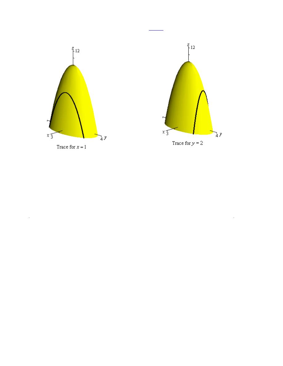
Example 2
Find the slopes of the traces to
2
2
10 4
z
x
y
=
-
-
at the point
( )
1, 2
.
Solution
We sketched the traces for the planes
1
x
=
and
2
y
=
in a previous
section
and these are the two
traces for this point. For reference purposes here are the graphs of the traces.
op
Next we’ll need the two partial derivatives so we can get the slopes.
( )
( )
,
8
,
2
x
y
f x y
x
f x y
y
= -
= -
To get the slopes all we need to do is evaluate the partial derivatives at the point in question.
( )
( )
1, 2
8
1, 2
4
x
y
f
f
= -
= -
So, the tangent line at
( )
1, 2
for the trace to
2
2
10 4
z
x
y
=
-
-
for the plane
2
y
=
has a slope of
-8. Also the tangent line at
( )
1, 2
for the trace to
2
2
10 4
z
x
y
=
-
-
for the plane
1
x
=
has a
sl e of -4.
6
Dr.Eng Muhammad.A.R.yass
Higher Order Partial Derivatives
Just as we had higher order derivatives with functions of one variable we will also have higher
order derivatives of functions of more than one variable. However, this time we will have more
options since we do have more than one variable..
Consider the case of a function of two variables,
( )
,
f x y
since both of the first order partial
derivatives are also functions of x and y we could in turn differentiate each with respect to x or y.
This means that for the case of a function of two variables there will be a total of four possible
second order derivatives. Here they are and the notations that we’ll use to denote them.
( )
( )
( )
( )
2
2
2
2
2
2
x
x x
x
x
x y
y
y
y x
x
y
y y
y
f
f
f
f
x
x
x
f
f
f
f
y
x
y x
f
f
f
f
x
y
x y
f
f
f
f
y
y
y
¶ 
æ
ö
=
=
=
ç
÷
è
ø
¶ 
æ
ö
=
=
=
ç
÷
¶ 
è
ø
æ
ö
¶ 
=
=
=
ç
÷
¶ 
è
ø
æ
ö
¶ 
=
=
=
ç
÷
è
ø
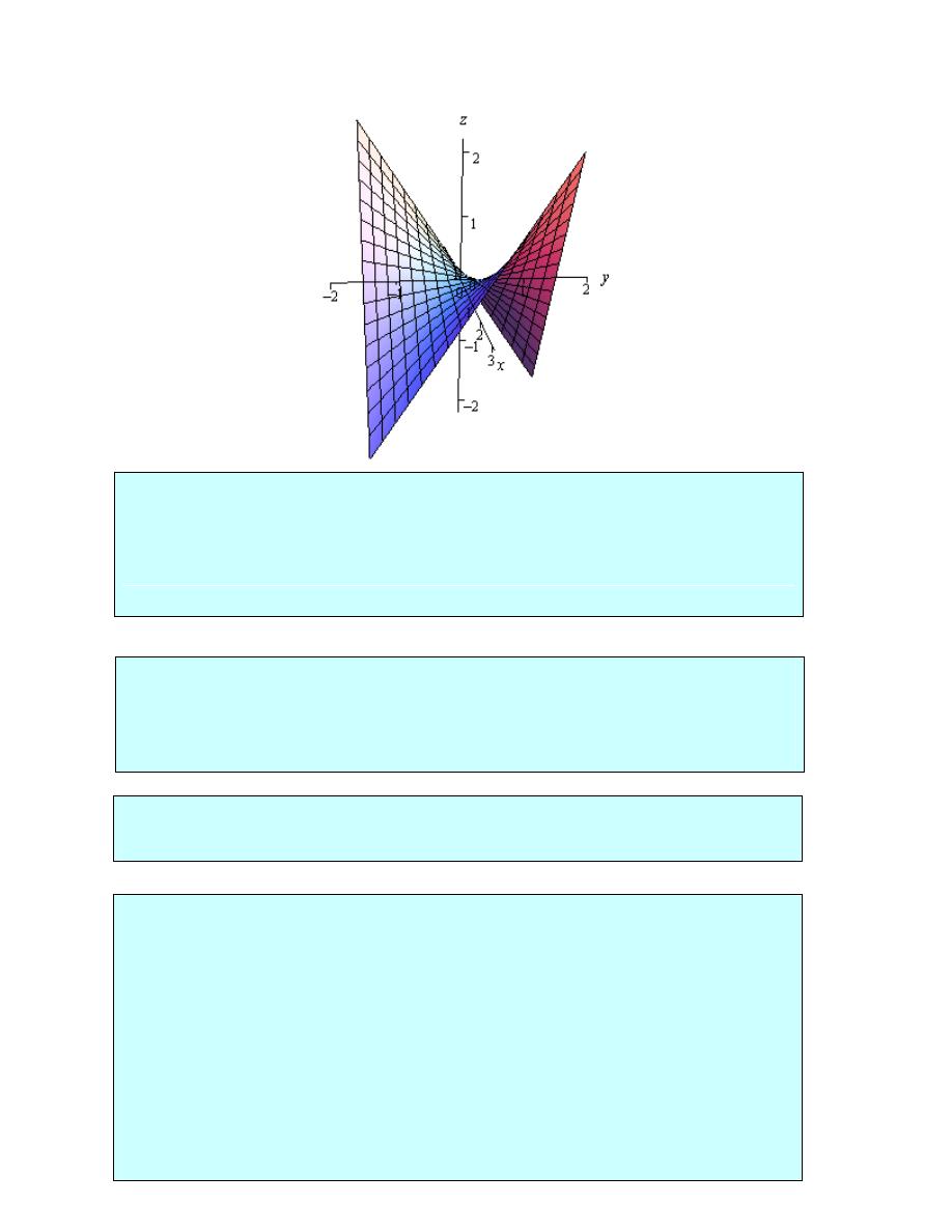
Example 1
Find all the second order derivatives for
( )
( )
2
2
5
,
cos 2
3
y
f x y
x
x
y
=
-
+
e
Solution
We’ll first need the first order derivatives so here they are.
( )
( )
( )
2
5
5
,
2sin 2
2
,
5
6
x
y
y
y
f x y
x
x
f x y
x
y
= -
-
= -
+
e
e
Now, let’s get the second order derivatives.
( )
2
5
5
5
5
4cos 2
2
10
10
25
6
xx
xy
yx
yy
y
y
y
y
f
x
f
x
f
x
f
x
= -
-
= -
= -
= -
+
e
e
e
e
Clairaut’s Theorem
Suppose that f is defined on a disk D that contains the point
( )
,
a b
. If the functions
xy
f
and
yx
f
are continuous on this disk then,
( )
( )
,
,
xy
yx
f
a b
f
a b
=
Example 2
Verify Clairaut’s Theorem for
( )
2 2
,
x y
f x y
x
-
= e
.
Solution
We’ll first need the two first order derivatives.
( )
( )
2 2
2 2
2 2
2
2
3
,
2
,
2
x
y
x y
x y
x y
f x y
x y
f x y
yx
-
-
-
=
-
= -
e
e
e
7
Dr.Eng Muhammad.A.R.yass
Now, compute the two fixed second order partial derivatives.
( )
( )
2 2
2 2
2 2
2 2
2 2
2 2
2 2
2
2
4 3
2
4 3
2
3 4
,
2
4
4
6
4
,
6
4
xy
yx
x y
x y
x y
x y
x y
x y
x y
f
x y
yx
x y
x y
x y
x y
f
x y
yx
y x
-
-
-
-
-
-
-
= -
-
+
= -
+
= -
+
e
e
e
e
e
e
e
Sure enough they are the same
( )
( )
2
3
2
3
2
x y x
xy x
y x x
yx x
f
f
f
f
x
y x
x y x
f
f
f
f
x
x y
x y
æ
ö
¶ 
=
=
=
ç
÷
¶ ¶ 
¶ ¶ 
è
ø
æ
ö
¶ 
=
=
=
ç
÷
¶ ¶ 
¶ 
è
ø
an extension to Clairaut’s Theorem that says if all three of these are continuous then they should
all be equal,
x x y
x y x
y x x
f
f
f
=
=
Example 3
Find the indicated derivative for each of the following functions.
(a) Find
x x y z z
f
for
(
)
( )
3 2
, ,
ln
f x y z
z y
x
=
(b) Find
3
2
f
y x
¶ 
for
( )
,
xy
f x y
= e
Solution
(a) Find
x x y z z
f
for
(
)
( )
3 2
, ,
ln
f x y z
z y
x
=
In this case remember that we differentiate from left to right. Here are the derivatives for this
part.
3 2
x
z y
f
x
=
3 2
2
xx
z y
f
x
= -
3
2
2
xxy
z y
f
x
= -
2
2
6
xxyz
z y
f
x
= -
2
12
xxyzz
zy
f
x
= -
(b) Find
3
2
f
y x
¶ 
for
( )
,
xy
f x y
= e
Here we differentiate from right to left. Here are the derivatives for this function.
xy
f
y
x
=
e
2
2
2
xy
f
y
x
=
e
3
2
2
2
xy
xy
f
y
xy
y x
=
+
¶ 
e
e
8
Dr.Eng Muhammad.A.R.yass
Differentials
This is a very short section and is here simply to acknowledge that just like we had
differentials
for functions of one variable we also have them for functions of more than one variable. Also, as
we’ve already seen in previous sections, when we move up to more than one variable things work
pretty much the same, but there are some small differences.
Given the function
( )
,
z
f x y
=
the differential dz or df is given by,
or
x
y
x
y
dz
f dx f dy
df
f dx f dy
=
+
=
+
There is a natural extension to functions of three or more variables. For instance, given the
function
(
)
, ,
w g x y z
=
the differential is given by,
x
y
z
dw g dx g dy g dz
=
+
+
Let’s do a couple of quick examples.
Example 1
Compute the differentials for each of the following functions.
(a)
( )
2
2
tan 2
x
y
z
x
+
= e
(b)
3 6
2
t r
u
s
=
Solution
(a)
( )
2
2
tan 2
x
y
z
x
+
= e
There really isn’t a whole lot to these outside of some quick differentiation. Here is the
differential for the function.
( )
( )
(
)
( )
2
2
2
2
2
2
2
2
tan 2
2
sec 2
2
tan 2
x
y
x
y
x
y
dz
x
x
x dx
y
x dy
+
+
+
=
+
+
e
e
e
(b)
3 6
2
t r
u
s
=
Here is the differential for this function.
2 6
3 5
3 6
2
2
3
3
6
2
t r
t r
t r
du
dt
dr
ds
s
s
s
=
+
-
9
Dr.Eng Muhammad.A.R.yass
Chain Rule
We’ve been using the standard chain rule for functions of one variable throughout the last couple
of sections. It’s now time to extend the chain rule out to more complicated situations. Before we
actually do that let’s first review the notation for the chain rule for functions of one variable.
The notation that’s probably familiar to most people is the following.
( )
( )
(
)
( )
( )
(
)
( )
F x
f g x
F x
f g x g x
¢
¢
¢
=
=
we are going to be using in this section. Here it is.
( )
( )
If
and
then
dy
dy dx
y
f x
x g t
dt
dx dt
=
=
=
Case 1 :
( )
,
z
f x y
=
,
( )
x g t
=
,
( )
y h t
=
and compute
dz
dt
.
This case is analogous to the standard chain rule from Calculus I that we looked at above. In this
case we are going to compute an ordinary derivative since z really would be a function of t only if
we were to substitute in for x and y.
The chain rule for this case is,
dz
f dx
f dy
dt
x dt
y dt
=
+
Example 1
Compute
dz
dt
for each of the following.
(a)
xy
z x
= e
,
2
x t
=
,
1
y t
-
=
(b)
2 3
cos
z x y
y
x
=
+
,
( )
2
ln
x
t
=
,
( )
sin 4
y
t
=
Solution
(a)
xy
z x
= e
,
2
x t
=
,
1
y t
-
=
There really isn’t all that much to do here other than using the formula.
(
)
( )
( )
(
)
2
2
2 2
2
2
xy
xy
xy
xy
xy
xy
dz
f dx
f dy
dt
x dt
y dt
yx
t
x
t
t
yx
t x
-
-
=
+
=
+
+
-
=
+
-
e
e
e
e
e
e
So, technically we’ve computed the derivative. However, we should probably go ahead and
substitute in for x and y as well at this point since we’ve already got t’s in the derivative. Doing
this gives,
(
)
2 4
2
2
2
t
t
t
t
t
dz
t
t
t t
t
t
dt
-
=
+
-
=
+
e
e
e
e
e
10

Dr.Eng Muhammad.A.R.yass
2
2
2
t
t
t
dz
z t
t
t
dt
=
Þ
=
+
e
e
e
The same result for less work. Note however, that often it will actually be more work to do the
substitution first.
(b)
2 3
cos
z x y
y
x
=
+
,
( )
2
ln
x
t
=
,
( )
sin 4
y
t
=
Okay, in this case it would almost definitely be more work to do the substitution first so we’ll use
the chain rule first and then substitute.
(
)
(
)
( )
(
)
( )
( )
( )
( )
( )
( )
(
)
3
2
2
3
2
2
2
2
2
2
2
2
sin
3
cos
4cos 4
4sin 4 ln
2sin 4 sin ln
4cos 4
3sin 4
ln
cos ln
dz
xy
y
x
x y
x
t
dt
t
t
t
t
t
t
t
t
t
t
æ ö
=
-
+
+
ç ÷
è ø
-
é
ù
=
+
+
ë
û
Now, there is a special case that we should take a quick look at before moving on to the next case.
Let’s suppose that we have the following situation,
( )
( )
,
z
f x y
y g x
=
=
In this case the chain rule for
dz
dx
becomes,
dz
f dx
f dy
f
f dy
dx
x dx
y dx
x
y dx
=
+
=
+
In the first term we are using the fact that,
( )
1
dx
d
x
dx
dx
=
=
Example 2
Compute
dz
dx
for
( )
3
ln
z x
xy
y
=
+
,
(
)
2
cos
1
y
x
=
+
Solution
We’ll just plug into the formula.
( )
(
)
(
)
(
)
(
)
(
)
(
)
(
)
(
)
(
)
(
)
(
)
(
)
2
2
2
2
2
2
2
2
2
2
2
2
2
ln
3
2 sin
1
ln
cos
1
1 2 sin
1
3cos
1
cos
1
ln
cos
1
1 2 tan
1
6 sin
1 cos
1
dz
y
x
xy
x
x
y
x
x
dx
xy
xy
x
x
x
x
x
x
x
x
x
x
x
x
x
x
æ
ö æ
ö
=
+
+
+
-
+
ç
÷ ç
÷
è
ø è
ø
æ
ö
ç
÷
=
+
+ -
+
+
+
ç
÷
+
è
ø
=
+
+ -
+ -
+
+
Now let’s take a look at the second case.
Case 2 :
( )
,
z
f x y
=
,
( )
,
x g s t
=
,
( )
,
y h s t
=
and compute
z
s
and
z
t
.
In this case if we were to substitute in for x and y we would get that z is a function of s and t and
so it makes sense that we would be computing partial derivatives here and that there would be
two of them.
Here is the chain rule for both of these cases.
z
f x
f y
z
f x
f y
s
x s
y s
t
x t
y t
¶ 
¶ 
¶ 
¶ 
=
+
=
+
¶ 
¶ 
¶ 
¶ 
11
Dr.Eng Muhammad.A.R.yass
Example 3
Find
z
s
and
z
t
for
( )
2
sin 3
r
z
q
= e
,
2
r st t
= -
,
2
2
s
t
q =
+
.
Solution
Here is the chain rule for
z
s
.
( )
(
)
( )
( )
(
)
(
)
(
)
(
)
(
)
2
2
2
2
2
2
2
2
2
2
2
2
2
2
2
sin 3
3
cos 3
3
cos 3
2
sin 3
r
r
st t
st t
z
s
t
s
s
t
s
s
t
t
s
t
s
t
q
q
-
-
=
+
+
+
æ
ö
=
+
+
ç
÷
è
ø
+
e
e
e
e
Now the chain rule for
z
t
.
( )
(
)
(
)
( )
(
)
(
)
(
)
(
)
(
)
(
)
2
2
2
2
2
2
2
2
2
2
2
2
2
2
2
sin 3
2
3
cos 3
3
cos 3
2
2
sin 3
r
r
st t
st t
z
t
s
t
t
s
t
t
s
t
s
t
s
t
s
t
q
q
-
-
=
-
+
+
+
æ
ö
= -
+
+
ç
÷
è
ø
+
e
e
e
e
Example 4
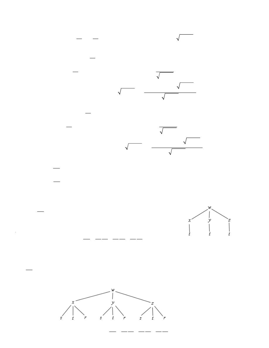
Use a tree diagram to write down the chain rule for the given derivatives.
(a)
dw
dt
for
(
)
, ,
w
f x y z
=
,
( )
1
x g t
=
,
( )
2
y g t
=
, and
( )
3
z g t
=
(b)
w
r
for
(
)
, ,
w
f x y z
=
,
(
)
1
, ,
x g s t r
=
,
(
)
2
, ,
y g s t r
=
, and
(
)
3
, ,
z g s t r
=
Solution
(a)
dw
dt
for
(
)
, ,
w
f x y z
=
,
( )
1
x g t
=
,
( )
2
y g t
=
, and
( )
3
z g t
=
So, we’ll first need the tree diagram so let’s get that.
dw
f dx
f dy
f dz
dt
x dt
y dt
z dt
=
+
+
which is really just a natural extension to the two variable case that we saw above.
(b)
w
r
for
(
)
, ,
w
f x y z
=
,
(
)
1
, ,
x g s t r
=
,
(
)
2
, ,
y g s t r
=
, and
(
)
3
, ,
z g s t r
=
Here is the tree diagram for this situation.
From this it looks like the derivative will be,
w
f x
f y
f z
r
x r
y r
z r
¶ 
¶ 
¶ 
=
+
+
¶ 
¶ 
¶ 
Return to Problems
12

Dr.Eng Muhammad.A.R.yass
Example 5
Compute
2
2
f
q
for
( )
,
f x y
if
cos
x r
q
=
and
sin
y r
q
=
.
Solution
We will need the first derivative before we can even think about finding the second derivative so
let’s get that. This situation falls into the second case that we looked at above so we don’t need a
new tree diagram. Here is the first derivative.
( )
( )
sin
cos
f
f x
f y
x
y
f
f
r
r
x
y
q
q
q
q
q
¶ 
¶ 
=
+
¶ 
¶ 
= -
+
Okay, now we know that the second derivative is,
( )
( )
2
2
sin
cos
f
f
f
f
r
r
x
y
q
q
q
q
q
q
æ
ö
¶ 
æ
ö
=
=
-
+
ç
÷
ç
÷
è
ø
è
ø
The issue here is to correctly deal with this derivative. Since the two first order derivatives,
f
x
and
f
y
, are both functions of x and y which are in turn functions of r and
q
both of these terms
are products. So, the using the product rule gives the following,
( )
( )
( )
( )
2
2
cos
sin
sin
cos
f
f
f
f
f
r
r
r
r
x
x
y
y
q
q
q
q
q
q
q
æ
ö
¶ 
¶ 
æ
ö
= -
-
-
+
ç
÷
ç
÷
è
ø
è
ø
We now need to determine what
f
x
q
¶ 
æ
ö
ç
÷
è
ø
and
f
y
q
æ
ö
¶ 
ç
÷
è
ø
will be. These are both chain rule
problems again since both of the derivatives are functions of x and y and we want to take the
derivative with respect to
q
.
Before we do these let’s rewrite the first chain rule that we did above a little.
( )
( ) ( )
( ) ( )
sin
cos
f
r
f
r
f
x
y
q
q
q
= -
+
(1)
Note that all we’ve done is change the notation for the derivative a little. With the first chain rule
written in this way we can think of (1) as a formula for differentiating any function of x and y
with respect to
q
provided we have
cos
x r
q
=
and
sin
y r
q
=
.
This however is exactly what we need to do the two new derivatives we need above. Both of the
first order partial derivatives,
f
x
and
f
y
, are functions of x and y and
cos
x r
q
=
and
sin
y r
q
=
so we can use (1) to compute these derivatives.
Here is the use of (1) to compute
f
x
q
¶ 
æ
ö
ç
÷
è
ø
.
( )
( )
( )
( )
2
2
2
sin
cos
sin
cos
f
f
f
r
r
x
x
x
y
x
f
f
r
r
x
y x
q
q
q
q
q
¶ 
¶ 
¶ 
æ
ö
æ
ö
æ
ö
= -
+
ç
÷
ç
÷
ç
÷
è
ø
è
ø
è
ø
= -
+
¶ 
Here is the computation for
f
y
q
æ
ö
¶ 
ç
÷
è
ø
.
13

Dr.Eng Muhammad.A.R.yass
( )
( )
( )
( )
2
2
2
sin
cos
sin
cos
f
f
f
r
r
y
x
y
y
y
f
f
r
r
x y
y
q
q
q
q
q
æ
ö
æ
ö
æ
ö
¶ 
¶ 
¶ 
= -
+
ç
÷
ç
÷
ç
÷
è
ø
è
ø
è
ø
= -
+
¶ 
The final step is to plug these back into the second derivative and do some simplifying.
( )
( )
( )
( )
( )
( )
( )
( )
( )
( )
( ) ( )
( )
( ) ( )
( )
( )
2
2
2
2
2
2
2
2
2
2
2
2
2
2
2
2
2
2
2
2
cos
sin
sin
cos
sin
cos
sin
cos
cos
sin
sin
cos
sin
sin
cos
cos
cos
s
f
f
f
f
r
r
r
r
x
x
y x
f
f
f
r
r
r
r
y
x y
y
f
f
f
r
r
r
x
x
y x
f
f
f
r
r
r
y
x y
y
f
r
r
x
q
q
q
q
q
q
q
q
q
q
q
q
q
q
q
q
q
q
æ
ö
= -
-
-
+
-
ç
÷
¶ 
è
ø
æ
ö
+
-
+
ç
÷
¶ 
è
ø
= -
+
-
-
¶ 
-
+
¶ 
= -
-
( )
( )
( ) ( )
( )
2
2
2
2
2
2
2
2
2
2
in
sin
2 sin
cos
cos
f
f
r
y
x
f
f
r
r
y x
y
q
q
q
q
q
+
-
+
¶ 
implicit differentiation
0
x
x
y
y
F
dy
dy
F
F
dx
dx
F
+
=
Þ
= -
Example 6
Find
dy
dx
for
( )
3 5
cos 3
3
xy
x
y
x y
x
+
=
- e
.
Solution
The first step is to get a zero on one side of the equal sign and that’s easy enough to do.
( )
3 5
cos 3
3
0
xy
x
y
x y
x
+
-
+
=
e
Now, the function on the left is
( )
,
F x y
in our formula so all we need to do is use the formula to
find the derivative.
( )
( )
2 5
3 4
cos 3
3
3
3 sin 3
5
xy
xy
y
x y
y
dy
dx
x
y
x y
x
+
- +
= -
-
+
+
e
e
Example 7
Find
z
x
and
z
y
for
(
)
( )
2
sin 2
5
1
cos 6
x
y
z
y
zx
-
= +
.
Solution
This was one of the functions that we used the old implicit differentiation on back in the
Partial
Derivatives
section. You might want to go back and see the difference between the two.
First let’s get everything on one side.
(
)
( )
2
sin 2
5
1
cos 6
0
x
y
z
y
zx
-
- -
=
Now, the function on the left is
(
)
, ,
F x y z
and so all that we need to do is use the formulas
developed above to find the derivatives.
(
)
( )
(
)
( )
2
2 sin 2
5
6 sin 6
5 cos 2
5
6
sin 6
x
y
z
yz
zx
z
x
x
y
z
yx
zx
-
+
= -
-
-
+
(
)
( )
(
)
( )
2
2
2 cos 2
5
cos 6
5 cos 2
5
6
sin 6
x
y
z
zx
z
y
x
y
z
yx
zx
-
-
= -
-
-
+
14

Dr.Eng Muhammad.A.R.yass
Directional Derivatives
To this point we’ve only looked at the two partial derivatives
( )
,
x
f x y
and
( )
,
y
f x y
. Recall
that these derivatives represent the rate of change of f as we vary x (holding y fixed) and as we
vary y (holding x fixed) respectively. We now need to discuss how to find the rate of change of f
if we allow both x and y to change simultaneously. The problem here is that there are many ways
to allow both x and y to change. For instance one could be changing faster than the other and
then there is also the issue of whether or not each is increasing or decreasing. So, before we get
into finding the rate of change we need to get a couple of preliminary ideas taken care of first.
The main idea that we need to look at is just how are we going to define the changing of x and/or
y.
Definition
The rate of change of
( )
,
f x y
in the direction of the unit vector
,
u
a b
=
r
is called the
directional derivative and is denoted by
( )
,
u
D f x y
r
. The definition of the directional
derivative is,
( )
(
)
( )
0
,
,
,
lim
h
u
f x ah y bh
f x y
D f x y
h
®
+
+
-
=
r
If we now go back to allowing x and y to be any number we get the following formula for
computing directional derivatives.
( )
( )
( )
,
,
,
x
y
u
D f x y
f x y a
f x y b
=
+
r
(
)
(
)
(
)
(
)
, ,
, ,
, ,
, ,
x
y
z
u
D f x y z
f x y z a
f x y z b f x y z c
=
+
+
r
Example 1
Find each of the directional derivatives.
(a)
( )
2,0
u
D f
r
where
( )
,
xy
f x y
x
y
=
+
e
and
ur
is the unit vector in the direction
of
2
3
p
q =
.
(b)
(
)
, ,
u
D f x y z
r
where
(
)
2
3 2
, ,
f x y z
x z y z
xyz
=
+
-
in the direction of
1,0,3
v
= -
r
.
Solution
(a)
( )
2,0
u
D f
r
where
( )
,
xy
f x y
x
y
=
+
e
and
ur
is the unit vector in the direction of
2
3
p
q =
.
We’ll first find
( )
,
u
D f x y
r
and then use this a formula for finding
( )
2,0
u
D f
r
. The unit vector
giving the direction is,
2
2
1
3
cos
,sin
,
3
3
2 2
u
p
p
æ
ö
æ
ö
=
= -
ç
÷
ç
÷
è
ø
è
ø
r
So, the directional derivative is,
( )
(
)
(
)
2
1
3
,
1
2
2
xy
xy
xy
u
D f x y
xy
x
æ
ö
æ
ö
= -
+
+
+
ç
÷
ç
÷
ç
÷
è
ø
e
e
e
r
è
ø
15
Dr.Eng Muhammad.A.R.yass
Now, plugging in the point in question gives,
( )
( )
( )
1
3
5 3 1
2,0
1
5
2
2
2
u
D f
æ
ö
-
æ
ö
= -
+
=
ç
÷
ç
÷
ç
÷
è
ø
è
ø
r
(b)
(
)
, ,
u
D f x y z
r
where
(
)
2
3 2
, ,
f x y z
x z y z
xyz
=
+
-
in the direction of
1,0,3
v
= -
r
.
In this case let’s first check to see if the direction vector is a unit vector or not and if it isn’t
convert it into one. To do this all we need to do is compute its magnitude.
1 0 9
10 1
v
=
+ + =
¹
r
So, it’s not a unit vector. Recall that we can convert any vector into a unit vector that points in
the same direction by dividing the vector by its magnitude. So, the unit vector that we need is,
1
1
3
1,0,3
,0,
10
10
10
u
=
-
= -
r
The directional derivative is then,
(
)
(
) ( )
(
)
(
)
(
)
2 2
2
3
2
3
1
3
, ,
2
0 3
2
10
10
1
3
6
3
2
10
u
D f x y z
xz yz
y z
xz
x
y z xy
x
y z
xy
xz yz
æ
ö
æ
ö
= -
-
+
-
+
+
-
ç
÷
ç
÷
è
ø
è
ø
=
+
-
-
+
r
(
)
(
)
(
)
(
)
, ,
, ,
, ,
, ,
, ,
, ,
x
y
z
x
y
z
u
D f x y z
f x y z a
f x y z b f x y z c
f f f
a b c
=
+
+
=
r
g
Now let’s give a name and notation to the first vector in the dot product since this vector will
show up fairly regularly throughout this course (and in other courses). The gradient of f or
gradient vector of f is defined to be,
, ,
or
,
x
y
z
x
y
f
f f f
f
f f
Ñ =
Ñ =
Or, if we want to use the standard basis vectors the gradient is,
or
x
y
z
x
y
f
f i
f j
f k
f
f i
f j
Ñ =
+
+
Ñ =
+
r
r
r
r
r
The definition is only shown for functions of two or three variables, however there is a natural
extension to functions of any number of variables that we’d like.
With the definition of the gradient we can now say that the directional derivative is given by,
u
D f
f u
= Ñ
r
r
g
where we will no longer show the variable and use this formula for any number of variables.
Note as well that we will sometimes use the following notation,
( )
u
D f x
f u
= Ñ
r
r
r
g
Example 2
Find each of the directional derivative.
(a)
( )
u
D f x
r
r
for
( )
( )
,
cos
f x y
x
y
=
in the direction of
2,1
v
=
r
.
(b)
( )
u
D f x
r
r
for
(
)
( )
( )
2
, ,
sin
ln
f x y z
yz
x
=
+
at
(
)
1,1,
p
in the direction of
1,1, 1
v
=
-
r
.
16
Dr.Eng Muhammad.A.R.yass
Solution
(a)
( )
u
D f x
r
r
for
( )
( )
,
cos
f x y
x
y
=
in the direction of
2,1
v
=
r
.
Let’s first compute the gradient for this function.
( )
( )
cos
,
sin
f
y
x
y
Ñ =
-
Also, as we saw earlier in this section the unit vector for this direction is,
2
1
,
5
5
u
=
r
The directional derivative is then,
( )
( )
( )
( )
( )
(
)
2
1
cos
,
sin
,
5
5
1
2cos
sin
5
u
D f x
y
x
y
y
x
y
=
-
=
-
r
r
g
(b)
( )
u
D f x
r
r
for
(
)
( )
( )
2
, ,
sin
ln
f x y z
yz
x
=
+
at
(
)
1,1,
p
in the direction of
1,1, 1
v
=
-
r
.
In this case are asking for the directional derivative at a particular point. To do this we will first
compute the gradient, evaluate it at the point in question and then do the dot product. So, let’s get
the gradient.
(
)
( )
( )
(
)
( )
( )
2
, ,
, cos
, cos
2
1,1,
, cos
,cos
2,
, 1
1
f x y z
z
yz y
yz
x
f
p
p
p
p
p
Ñ
=
Ñ
=
=
- -
Next, we need the unit vector for the direction,
1
1
1
3
,
,
3
3
3
v
u
=
=
-
r
r
Finally, the directional derivative at the point in question is,
(
)
(
)
1
1
1
1,1,
2,
, 1
,
,
3
3
3
1
2
1
3
3
3
u
D f
p
p
p
p
=
- -
-
=
- +
-
=
r
g
Theorem
The maximum value of
( )
u
D f x
r
r
(and hence then the maximum rate of change of the function
( )
f xr
) is given by
( )
f x
Ñ r
and will occur in the direction given by
( )
f x
Ñ r
.
The maximum rate of change of the elevation will then occur in the direction of
(
)
60,100
1.2, 4
f
Ñ
= -
-
Example 3
Suppose that the height of a hill above sea level is given by
2
2
1000 0.01
0.02
z
x
y
=
-
-
. If you are at the point
(
)
60,100
in what direction is the elevation
changing fastest? What is the maximum rate of change of the elevation at this point?
Solution
Now on to the problem. There are a couple of questions to answer here, but using the theorem
makes answering them very simple. We’ll first need the gradient vector.
( )
0.02 , 0.04
f x
x
y
Ñ
= -
-
r
The maximum rate of change of the elevation will then occur in the direction of
(
)
60,100
1.2, 4
f
Ñ
= -
-
The maximum rate of change of the elevation at this point is,
(
)
(
) ( )
2
2
60,100
1.2
4
17.44 4.176
f
Ñ
=
-
+
=
=
17
Dr.Eng Muhammad.A.R.yass
Applications of Partial Derivatives
18
Dr.Eng Muhammad.A.R.yass
The equation of the tangent plane to the surface given by
( )
,
z
f x y
=
at
(
)
0
0
,
x y
is then,
(
)(
)
(
)(
)
0
0
0
0
0
0
0
,
,
x
y
z z
f x y
x x
f x y
y y
-
=
-
+
-
Also, if we use the fact that
(
)
0
0
0
,
z
f x y
=
we can rewrite the equation of the tangent plane as,
(
)
(
)(
)
(
)(
)
(
)
(
)(
)
(
)(
)
0
0
0
0
0
0
0
0
0
0
0
0
0
0
0
0
,
,
,
,
,
,
x
y
x
y
z
f x y
f x y
x x
f x y
y y
z
f x y
f x y
x x
f x y
y y
-
=
-
+
-
=
+
-
+
-
Example 1
Find the equation of the tangent plane to
(
)
ln 2
z
x y
=
+
at
(
)
1,3
-
.
Solution
Tangent Planes and Linear Approximations
( )
(
)
(
)
( )
( )
(
)
( )
(
)
0
,
ln 2
1,3
ln 1
0
2
,
1,3
2
2
1
,
1,3
1
2
x
x
y
y
f x y
x y
z
f
f x y
f
x y
f x y
f
x y
=
+
=
-
=
=
=
-
=
+
=
-
=
+
The equation of the plane is then,
(
) ( )(
)
0 2
1
1
3
z
x
y
- =
+ +
-
2
1
z
x y
=
+ -
linear approximation to be,
One nice use of tangent planes is they give us a way to approximate a surface near a point. As
long as we are near to the point
(
)
0
0
,
x y
then the tangent plane should nearly approximate the
function at that point. Because of this
defi
h li ear app
im i
b
( )
(
)
(
)(
)
(
)(
)
0
0
0
0
0
0
0
0
,
,
,
,
x
y
L x y
f x y
f x y
x x
f x y
y y
=
+
-
+
-
and as long as we are “near”
(
)
0
0
,
x y
then we should have that,
( )
( )
(
)
(
)(
)
(
)(
)
0
0
0
0
0
0
0
0
,
,
,
,
,
x
y
f x y
L x y
f x y
f x y
x x
f x y
y y
»
=
+
-
+
-
we
ne t e n
rox
at on to e,
19
Dr.Eng Muhammad.A.R.yass
Example 2
Find the linear approximation to
2
2
3
16
9
x
y
z
= +
+
at
(
)
4,3
-
.
Solution
So, we’re really asking for the tangent plane so let’s find that.
( )
(
)
( )
(
)
( )
(
)
2
2
,
3
4,3
3 1 1 5
16
9
1
,
4,3
8
2
2
2
,
4,3
9
3
x
x
y
y
x
y
f x y
f
x
f x y
f
y
f x y
f
= +
+
-
= + + =
=
-
= -
=
-
=
The tangent plane, or linear approximation, is then,
( )
(
)
(
)
1
2
,
5
4
3
2
3
L x y
x
y
= -
+ +
-
Gradient Vector, Tangent Planes and Normal Lines
The equation of the tangent plane is then,
(
)(
)
(
)(
) (
)
0
0
0
0
0
0
0
,
,
0
x
y
f x y
x x
f x y
y y
z z
-
+
-
- -
=
Or, upon solving for z, we get,
(
)
(
)(
)
(
)(
)
0
0
0
0
0
0
0
0
,
,
,
x
y
z
f x y
f x y
x x
f x y
y y
=
+
-
+
-
the equation of the normal line is,
( )
(
)
0
0
0
0
0
0
, ,
, ,
r t
x y z
t f x y z
=
+ Ñ
r
Example 1
Find the tangent plane and normal line to
2
2
2
30
x
y
z
+
+
=
at the point
(
)
1, 2,5
-
.
Solution
For this case the function that we’re going to be working with is,
(
)
2
2
2
, ,
F x y z
x
y
z
=
+
+
and note that we don’t have to have a zero on one side of the equal sign. All that we need is a
constant. To finish this problem out we simply need the gradient evaluated at the point.
(
)
2 , 2 , 2
1, 2,5
2, 4,10
F
x y z
F
Ñ =
Ñ
-
=
-
The tan ent lane is the
g
p
n,
(
) (
)
(
)
2
1
4
2
10
5
0
x
y
z
- -
+ +
- =
The normal line is,
( )
1, 2,5
2, 4,10
1 2 , 2 4 ,5 10
r t
t
t
t
t
=
-
+
-
= +
- -
+
r
20
Dr.Eng Muhammad.A.R.yass
Relative Minimums and Maximums
Definition
1. A function
( )
,
f x y
has a relative minimum at the point
( )
,
a b
if
( )
( )
,
,
f x y
f a b
³
for
all points
( )
,
x y
in some region around
( )
,
a b
.
2. A function
( )
,
f x y
has a relative maximum at the point
( )
,
a b
if
( )
( )
,
,
f x y
f a b
£
for
all points
( )
,
x y
in some region around
( )
,
a b
.
Definition
The point
( )
,
a b
is a critical point (or a stationary point) of
( )
,
f x y
provided one of the
following is true,
1.
( )
,
0
f a b
Ñ
=
r
(this is equivalent to saying that
( )
,
0
x
f a b
=
and
( )
,
0
y
f a b
=
),
2.
( )
,
x
f a b
and/or
( )
,
y
f a b
doesn’t exist.
Fact
If the point
( )
,
a b
is a relative extrema of the function
( )
,
f x y
then
( )
,
a b
is also a critical
point of
( )
,
f x y
and in fact we’ll have
( )
,
0
f a b
Ñ
=
r
.
Fact
Suppose that
( )
,
a b
is a critical point of
( )
,
f x y
and that the second order partial derivatives are
continuous in some region that contains
( )
,
a b
. Next define,
( )
( ) ( )
( )
2
,
,
,
,
x x
y y
x y
D D a b
f
a b f
a b
f
a b
é
ù
=
=
- ë
û
We then have the following classifications of the critical point.
1. If
0
D
>
and
( )
,
0
x x
f
a b
>
then there is a relative minimum at
( )
,
a b
.
2. If
0
D
>
and
( )
,
0
x x
f
a b
<
then there is a relative maximum at
( )
,
a b
.
3. If
0
D
<
then the point
( )
,
a b
is a saddle point.
4. If
0
D
=
then the point
( )
,
a b
may be a relative minimum, relative maximum or a
saddle point. Other techniques would need to be used to classify the critical point.
21

Dr.Eng Muhammad.A.R.yass
Example 1
Find and classify all the critical points of
( )
3
3
,
4
3
f x y
x
y
xy
= +
+
-
.
Solution
We first need all the first order (to find the critical points) and second order (to classify the
critical points) partial derivatives so let’s get those.
2
2
3
3
3
3
6
6
3
x
y
x x
y y
x y
f
x
y
f
y
x
f
x
f
y
f
=
-
=
-
=
=
= -
Let’s first find the critical points. Critical points will be solutions to the system of equations,
2
2
3
3
0
3
3
0
x
y
f
x
y
f
y
x
=
-
=
=
-
=
This is a non-linear system of equations and these can, on occasion, be difficult to solve.
However, in this case it’s not too bad. We can solve the first equation for y as follows,
2
2
3
3
0
x
y
y x
-
=
Þ
=
Plugging this into the second equation gives,
( )
(
)
2
2
3
3
3
3
1
0
x
x
x x
-
=
- =
From this we can see that we must have
0
x
=
or
1
x
=
. Now use the fact that
2
y x
=
to get the
critical points.
( )
( )
2
2
0 :
0
0
0,0
1:
1
1
1,1
x
y
x
y
=
=
=
Þ
=
= =
Þ
So, we get two critical points. All we need to do now is classify them. To do this we will need
D. Here is the general formula for D.
( )
( ) ( )
( )
( )( ) ( )
2
2
,
,
,
,
6
6
3
36
9
x x
y y
x y
D x y
f
x y f
x y
f
x y
x
y
xy
é
ù
=
- ë
û
=
- -
=
-
To classify the critical points all that we need to do is plug in the critical points and use the fact
above to classify them.
( )
0,0
:
( )
0,0
9 0
D D
=
= - <
So, for
( )
0,0
D is negative and so this must be a saddle point.
p
g ph o
( )
1,1
:
( )
( )
1,1
36 9 27 0
1,1
6 0
x x
D D
f
=
=
- =
>
= >
For
( )
1,1
D is positive and
x x
f
is positive and so we must have a relative minimum.
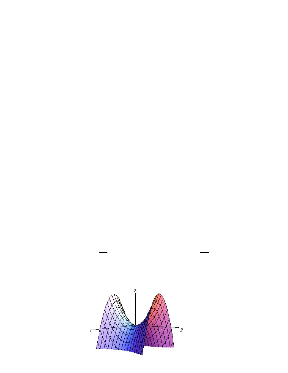
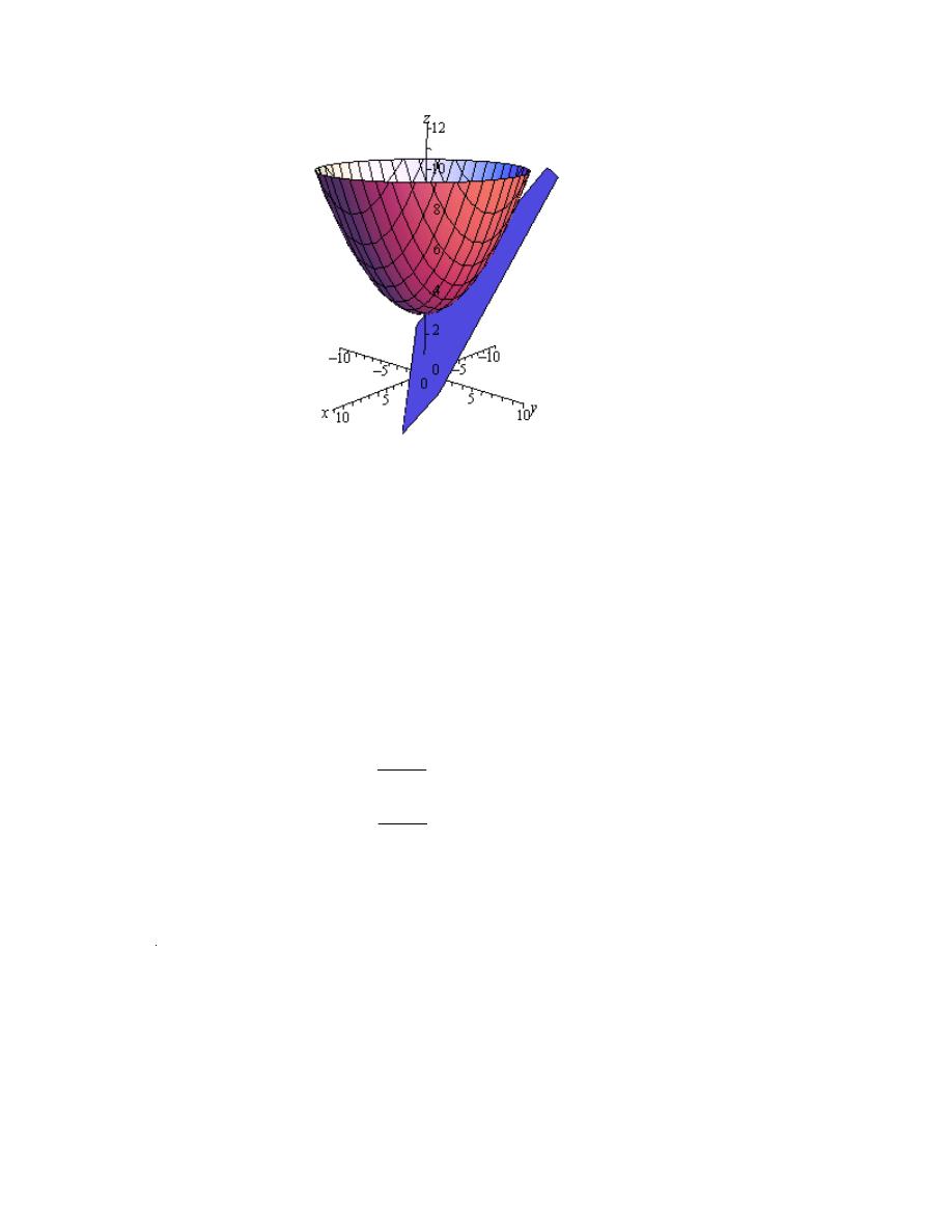
For the sake of com leteness here is a ra
f this function.
22
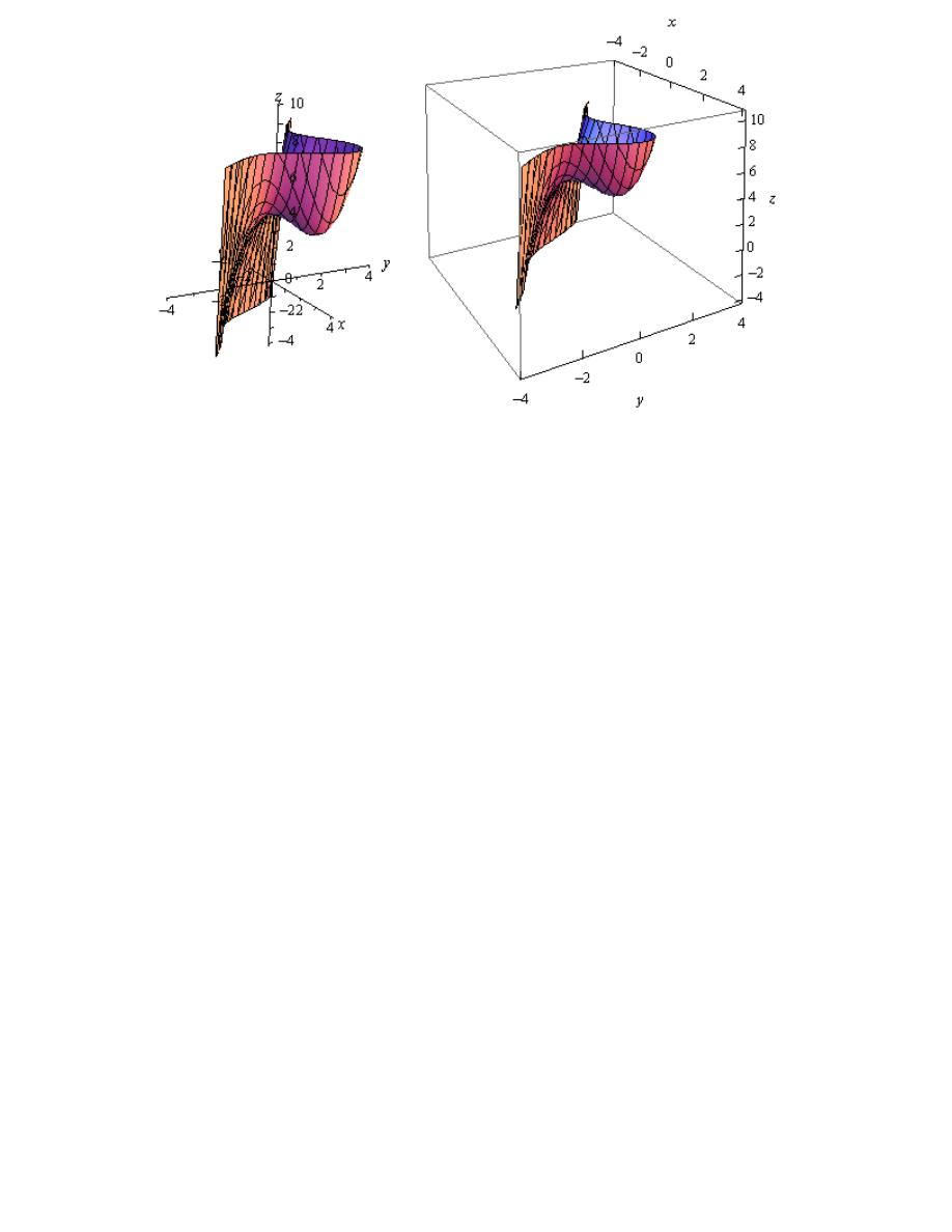
Dr.Eng Muhammad.A.R.yass
Notice that in order to get a better visual we used a somewhat nonstandard orientation. We can
ee that there is a relative minimum at
( )
1,1
and (hopefully) it’s clear that at
( )
0,0
we do get a
addle point.
s
s
Example 2
Find and classify all the critical points for
( )
2
3
2
2
,
3
3
3
2
f x y
x y y
x
y
=
+
-
-
+
Solution
As with the first example we will first need to get all the first and second order derivatives.
2
2
6
6
3
3
6
6
6
6
6
6
x
y
x x
y y
x y
f
xy
x
f
x
y
y
f
y
f
y
f
x
=
-
=
+
-
=
-
=
-
=
We’ll first need the critical points. The equations that we’ll need to solve this time are,
2
2
6
6
0
3
3
6
0
xy
x
x
y
y
-
=
+
-
=
These equations are a little trickier to solve than the first set, but once you see what to do they
really aren’t terribly bad.
First, let’s notice that we can factor out a 6x from the first equation to get,
(
)
6
1
0
x y
- =
So, we can see that the first equation will be zero if
0
x
=
or
1
y
=
. Be careful to not just cancel
the x from both sides. If we had done that we would have missed
0
x
=
.
To find the critical points we can plug these (individually) into the second equation and solve for
the
remaining
variable
.
0
x
=
:
(
)
3
6
3
2
0
0,
2
y
y
y y
y
y
-
=
-
=
Þ
=
=
1
y
=
:
(
)
2
2
3
3 3
1
0
1,
1
x
x
x
x
- =
- =
Þ
= -
=
So, if
0
x
=
we have the following critical points,
( ) ( )
0,0
0, 2
and if
1
y
=
the critical points are,
( ) (
)
1,1
1,1
-
Now all we need to do is classify the critical points. To do this we’ll need the general formula for
D.
( ) (
)(
) ( ) (
)
2
2
2
,
6
6 6
6
6
6
6
36
D x y
y
y
x
y
x
=
-
- -
=
-
-
( )
0,0
:
23
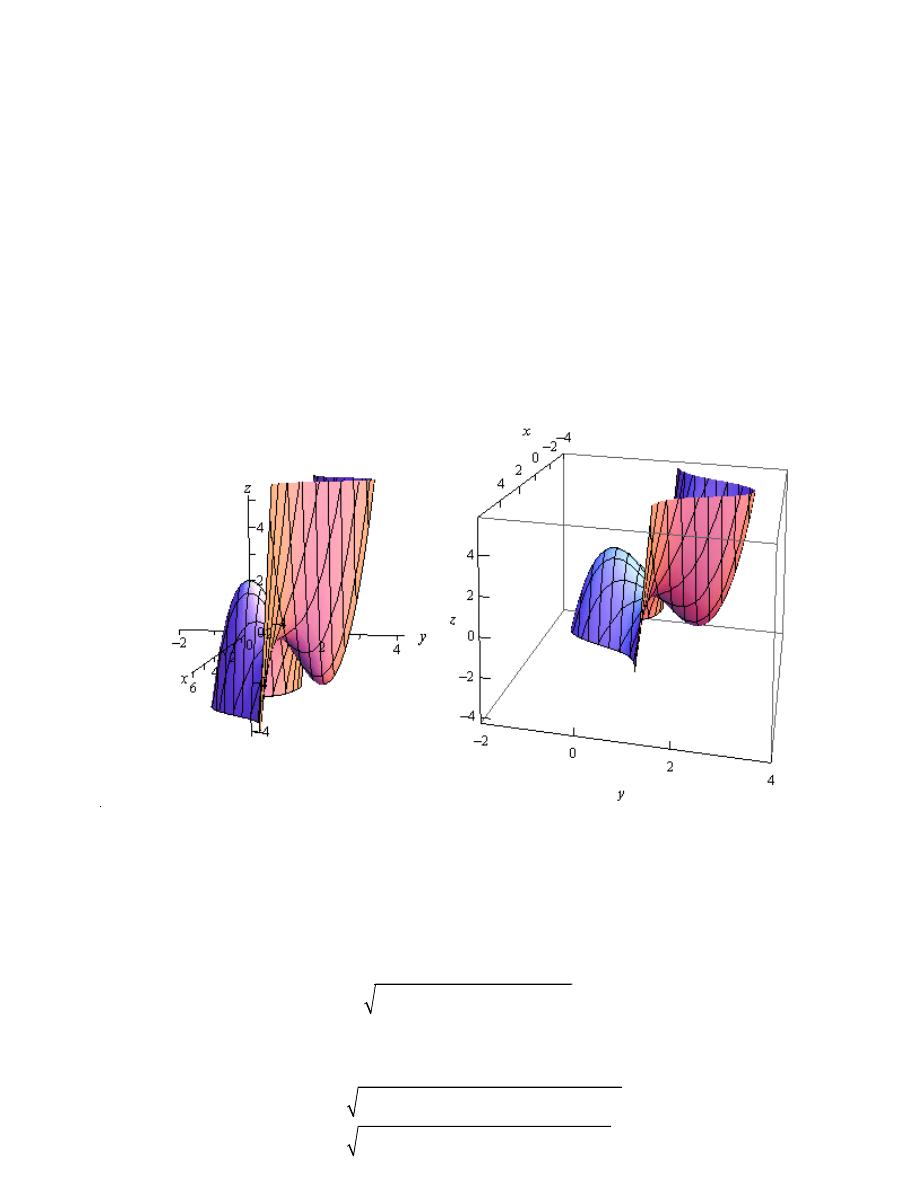
Dr.Eng Muhammad.A.R.yass
( )
( )
0,0
36 0
0,0
6 0
x x
D D
f
=
=
>
= - <
( )
0, 2
:
( )
( )
0, 2
36 0
0, 2
6 0
x x
D D
f
=
=
>
= >
( )
1,1
:
( )
1,1
36 0
D D
=
= - <
(
)
1,1
-
:
(
)
1,1
36 0
D D
=
-
= - <
So, it looks like we have the following classification of each of these critical points.
( )
( )
( )
(
)
0,0
: Relative Maximum
0, 2
: Relative Minimum
1,1
: Saddle Point
1,1 : Saddle Point
-
Here is a graph of the surface for the sake of completeness.
Example 3
Determine the point on the plane
4
2
1
x
y z
-
+ =
that is closest to the point
(
)
2, 1,5
- -
.
Solution
First, let’s suppose that
(
)
, ,
x y z
is any point on the plane. The distance between this point and
the point in question,
(
)
2, 1,5
- -
, is given by the formula,
(
) (
) (
)
2
2
2
2
1
5
d
x
y
z
=
+
+
+
+ -
equation of the plane to see that,
1 4
2
z
x
y
= -
+
Plugging this into the distance formula gives,
(
) (
) (
)
(
) (
) (
)
2
2
2
2
2
2
2
1
1 4
2
5
2
1
4 4
2
d
x
y
x
y
x
y
x
y
=
+
+
+
+ -
+
-
=
+
+
+
+ - -
+
24
Dr.Eng Muhammad.A.R.yass
So, let’s instead find the minimum value of
( )
(
) (
) (
)
2
2
2
2
,
2
1
4 4
2
f x y
d
x
y
x
y
=
=
+
+
+
+ - -
+
that is closest to
(
)
2, 1,5
- -
.
We’ll need the derivatives first.
(
) ( )(
)
(
) ( )(
)
2
2
2 4
4 4
2
36 34
16
2
1
2 2
4 4
2
14 16
10
34
10
16
x
y
x x
y y
x y
f
x
x
y
x
y
f
y
x
y
x
y
f
f
f
=
+ + -
- -
+
=
+
-
=
+ +
- -
+
= - -
+
=
=
= -
Now, before we get into finding the critical point let’s compute D quickly.
( ) (
)
2
34 10
16
84 0
D
=
- -
=
>
So, in this case D will always be positive and also notice that
34 0
x x
f
=
>
is always positive a
so any critical points that we get will be guaranteed to be relative minimums.
Now let’s find the critical point(s). This will mean solving the system.
36 34
16
0
14 16
10
0
x
y
x
y
+
-
=
- -
+
=
To do this we can solve the first equation for x.
(
)
(
)
1
1
16
36
8
18
34
17
x
y
y
=
-
=
-
Now, plug this into the second equation and solve for y.
(
)
16
25
14
8
18
10
0
17
21
y
y
y
- -
-
+
=
Þ
= -
Back substituting this into the equation for x gives
34
21
x
= -
.
So, it looks like we get a single critical point :
(
)
34
25
21
21
,
-
-
.
nd
34
25
107
1 4
2
21
21
21
z
æ
ö
æ
ö
= -
-
+
-
=
ç
÷
ç
÷
è
ø
è
ø
So, the point on the plane that is closest to
(
)
2, 1,5
- -
is
(
)
34
25 107
21
21
21
,
,
-
-
.
25

Dr.Eng Muhammad.A.R.yass
Absolute Minimums and Maximums
In this section we are going to extend the work from the previous section. In the previous section
we were asked to find and classify all critical points as relative minimums, relative maximums
and/or saddle points. In this section we want to optimize a function, that is identify the absolute
minimum and/or the absolute maximum of the function, on a given region in
2
¡
. Note that
when we say we are going to be working on a region in
2
¡
we mean that we’re going to be
looking at some region in the xy-plane.
In order to optimize a function in a region we are going to need to get a couple of definitions out
of the way and a fact. Let’s first get the definitions out of the way.
Definitions
1. A region in
2
¡
is called closed if it includes its boundary. A region is called open if it
doesn’t include any of its boundary points.
2. A region in
2
¡
is called bounded if it can be completely contained in a disk. In other
words, a region will be bounded if it is finite.
Let’s think a little more about the definition of closed. We said a region is closed if it includes its
boundary. Just what does this mean? Let’s think of a rectangle. Below are two definitions of a
rectangle, one is closed and the other is open.
Open
Closed
5
3
5
3
1
6
1
6
x
x
y
y
- < <
- £ £
< <
£ £
In this first case we don’t allow the ranges to include the endpoints (i.e. we aren’t including the
edges of the rectangle) and so we aren’t allowing the region to include any points on the edge of
the rectangle. In other words, we aren’t allowing the region to include its boundary and so it’s
open.
In the second case we are allowing the region to contain points on the edges and so will contain
its entire boundary and hence will be closed.
This is an important idea because of the following fact.
Extreme Value Theorem
If
( )
,
f x y
is continuous in some closed, bounded set D in
2
¡
then there are points in D,
(
)
1
1
,
x y
and
(
)
2
2
,
x y
so that
(
)
1
1
,
f x y
is the absolute maximum and
(
)
2
2
,
f x y
is the absolute
minimum of the function in D.
Note that this theorem does NOT tell us where the absolute minimum or absolute maximum will
occur. It only tells us that they will exist. Note as well that the absolute minimum and/or
absolute maximum may occur in the interior of the region or it may occur on the boundary of the
region.
26
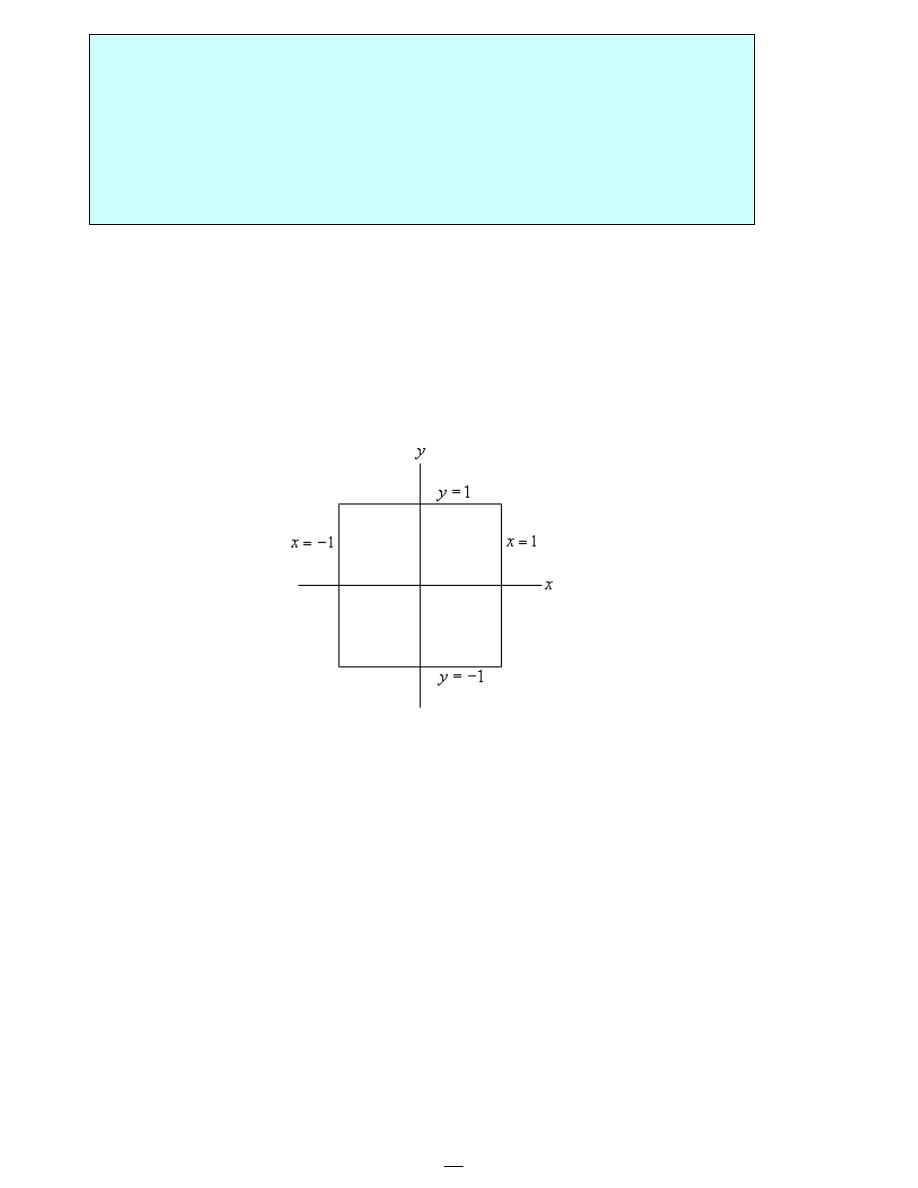
Dr.Eng Muhammad.A.R.yass
Finding Absolute Extrema
1. Find all the critical points of the function that lie in the region D and determine the function
value at each of these points.
2. Find all extrema of the function on the boundary.
3. The largest and smallest values found in the first two steps are the absolute minimum and the
absolute maximum of the function.
The main difference between this process and the process that we used in Calculus I is that the
“boundary” in Calculus I was just two points and so there really wasn’t a lot to do in the second
step. For these problems the majority of the work is often in the second step as we will often end
up doing a Calculus I absolute extrema problem one or more times.
Example 1
Find the absolute minimum and absolute maximum of
( )
2
2
2
,
4
2
4
f x y
x
y
x y
=
+
-
+
on the rectangle given by
1
1
x
- £ £
and
1
1
y
- £ £
.
Solution
Let’s first get a quick picture of the rectangle for reference purposes.
The boundary of this rectangle is given by the following conditions
right side :
1, 1
1
left side :
1, 1
1
upper side :
1, 1
1
lower side :
1, 1
1
x
y
x
y
y
x
y
x
= - £ £
= - - £ £
= - £ £
= - - £ £
These will be important in the second step of our process.
We’ll start this off by finding all the critical points that lie inside the given rectangle. To do this
we’ll need the two first order derivatives.
2
2
4
8
2
x
y
f
x
xy
f
y
x
=
-
=
-
Note that since we aren’t going to be classifying the critical points we don’t need the second
order derivatives. To find the critical points we will need to solve the system,
2
2
4
0
8
2
0
x
xy
y
x
-
=
-
=
We can solve the second equation for y to get,
2
4
x
y
=
27

Dr.Eng Muhammad.A.R.yass
Plugging this into the first equation gives us,
(
)
2
3
2
2
4
2
2
0
4
x
x
x
x x
x
x
æ
ö
-
=
-
=
-
=
ç
÷
è
ø
This tells us that we must have
0
x
=
or
2
1.414...
x
= ±
= ±
. Now, recall that we only want
critical points in the region that we’re given. That means that we only want critical points for
which
1
1
x
- £ £
. The only value of x that will satisfy this is the first one so we can ignore the
last two for this problem. Note however that a simple change to the boundary would include
these two so don’t forget to always check if the critical points are in the region (or on the
boundary since that can also happen).
Plugging
0
x
=
into the equation for y gives us,
2
0
0
4
y
=
=
The single critical point, in the region (and again, that’s important), is
( )
0,0
. We now need to
get the value of the function at the critical point.
( )
0,0
4
f
=
Eventually we will compare this to values of the function found in the next step and take the
largest and smallest as the absolute extrema of the function in the rectangle.
Now we have reached the long part of this problem. We need to find the absolute extrema of the
function along the boundary of the rectangle. What this means is that we’re going to need to look
at what the function is doing along each of the sides of the rectangle listed above.
Let’s first take a look at the right side. As noted above the right side is defined by
1, 1
1
x
y
= - £ £
Notice that along the right side we know that
1
x
=
. Let’s take advantage of this by defining a
new function as follows,
( )
( )
( )
2
2
2
2
1,
1
4
2 1
4 5 4
2
g y
f
y
y
y
y
y
=
= +
-
+ = +
-
Now, finding the absolute extrema of
( )
,
f x y
along the right side will be equivalent to finding
the absolute extrema of
( )
g y
in the range
1
1
y
- £ £
. Hopefully you
recall
how to do this from
Calculus I. We find the critical points of
( )
g y
in the range
1
1
y
- £ £
and then evaluate
( )
g y
at the critical points and the end points of the range of y’s.
Let’s do that for this problem.
( )
1
8
2
4
g y
y
y
¢
=
-
Þ
=
This is in the range and so we will need the following function evaluations.
( )
( )
1
19
1
11
1
7
4.75
4
4
g
g
g
æ ö
- =
=
=
=
ç ÷
è ø
Notice that, using the definition of
( )
g y
these are also function values for
( )
,
f x y
.
28
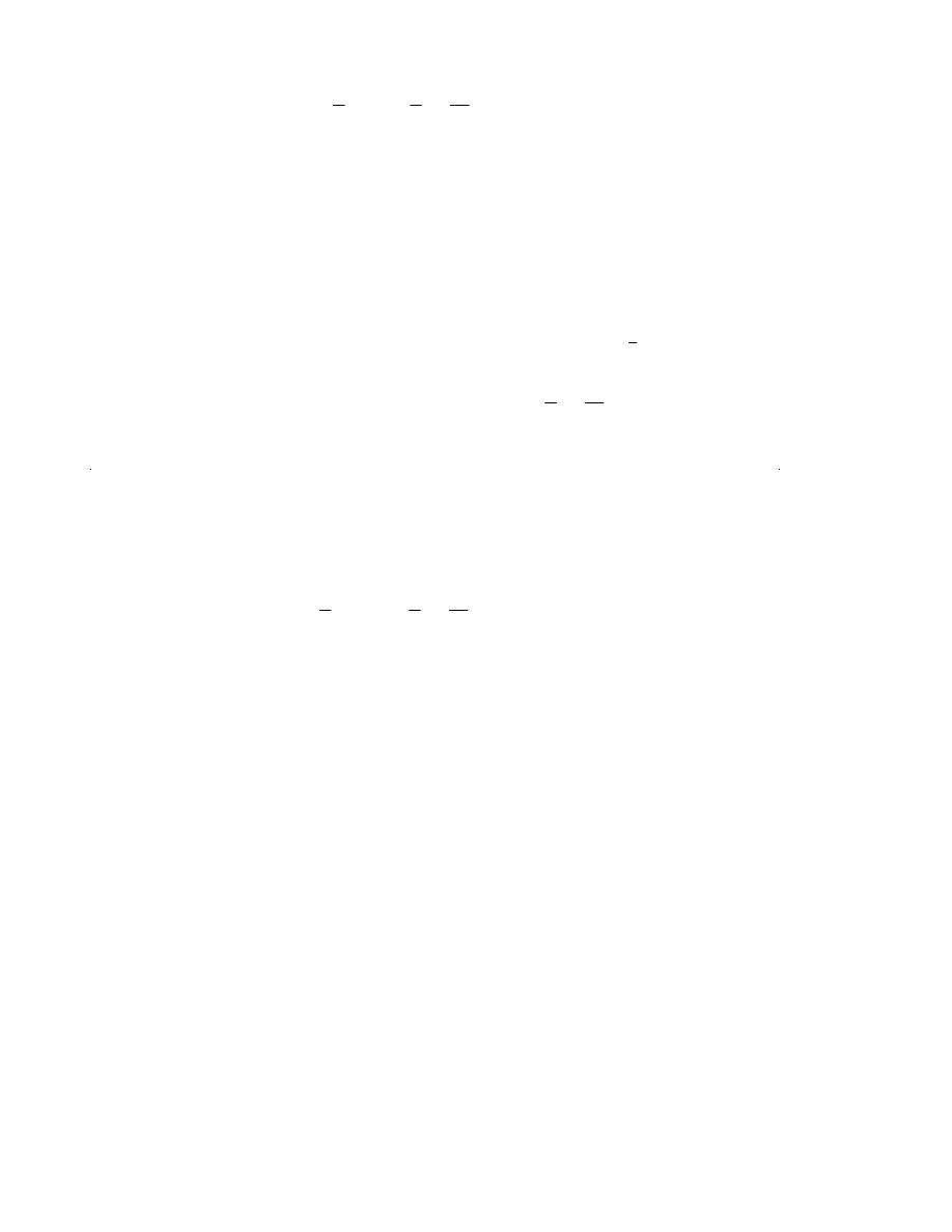
Dr.Eng Muhammad.A.R.yass
( )
(
)
( )
( )
1
1, 1
11
1
1,1
7
1
1
19
1,
4.75
4
4
4
g
f
g
f
g
f
- =
- =
=
=
æ ö
æ
ö
=
=
=
ç ÷
ç
÷
è ø
è
ø
We can now do the left side of the rectangle which is defined by,
1, 1
1
x
y
= - - £ £
Again, we’ll define a new function as follows,
( )
(
) ( )
( )
2
2
2
2
1,
1
4
2 1
4 5 4
2
g y
f
y
y
y
y
y
=
-
= -
+
- -
+ = +
-
Notice however that, for this boundary, this is the same function as we looked at for the right
side. This will not always happen, but since it has let’s take advantage of the fact that we’ve
already done the work for this function. We know that the critical point is
1
4
y
=
and we know
that the function value at the critical point and the end points are,
( )
( )
1
19
1
11
1
7
4.75
4
4
g
g
g
æ ö
- =
=
=
=
ç ÷
è ø
The only real difference here is that these will correspond to values of
,
f x y
at different points
( )
than for the right side. In this case these will correspond to the following function values for
( )
,
f x y
.
( )
(
)
( )
(
)
1
1, 1
11
1
1,1
7
1
1
19
1,
4.75
4
4
4
g
f
g
f
g
f
- =
- - =
=
-
=
æ ö
æ
ö
=
-
=
=
ç ÷
ç
÷
è ø
è
ø
We can now look at the upper side defined by,
1, 1
1
y
x
= - £ £
We’ll again define a new function except this time it will be a function of x.
( )
( )
( )
( )
2
2
2
2
,1
4 1
2
1
4 8
h x
f x
x
x
x
=
=
+
-
+ = -
We need to find the absolute extrema of
( )
h x
on the range
1
1
x
- £ £
. First find the critical
point(s).
( )
2
0
h x
x
x
¢
= -
Þ
=
The value of this function at the critical point and the end points is,
( )
( )
( )
1
7
1
7
0
8
h
h
h
- =
=
=
and these in turn correspond to the following function values for
( )
,
f x y
( )
(
)
( )
( )
( )
( )
1
1,1
7
1
1,1
7
0
0,1
8
h
f
h
f
h
f
- =
-
=
=
=
=
=
Note that there are several “repeats” here. The first two function values have already been
computed when we looked at the right and left side. This will often happen.
Finally, we need to take care of the lower side. This side is defined by,
1, 1
1
y
x
= - - £ £
29
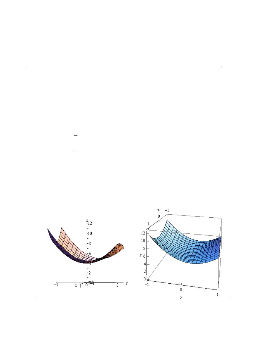
Dr.Eng Muhammad.A.R.yass
The new function we’ll define in this case is,
( )
(
)
( )
( )
2
2
2
2
, 1
4 1
2
1
4 8 3
h x
f x
x
x
x
=
- =
+ -
-
- + = +
The critical point for this function is,
( )
6
0
h x
x
x
¢
=
Þ
=
The function values at the critical point and the endpoint are,
( )
( )
( )
1
11
1
11
0
8
h
h
h
- =
=
=
and the corresponding values for
( )
,
f x y
are,
( )
(
)
( )
(
)
( )
(
)
1
1, 1
11
1
1, 1
11
0
0, 1
8
h
f
h
f
h
f
- =
- - =
=
- =
=
- =
The final step to this (long…) process is to collect up all the function values for
( )
,
f x y
that
we’ve computed in this problem. Here they are,
( )
(
)
( )
(
)
(
)
( )
(
)
0,0
4
1, 1
11
1,1
7
1
1,
4.75
1,1
7
1, 1
11
4
1
1,
4.75
0,1
8
0, 1
8
4
f
f
f
f
f
f
f
f
f
=
- =
=
æ
ö =
-
=
- - =
ç
÷
è
ø
æ
ö
-
=
=
- =
ç
÷
è
ø
The absolute minimum is at
( )
0,0
since gives the smallest function value and the absolute
maximum occurs at
(
)
1, 1
-
and
(
)
1, 1
- -
since these two points give the largest function value.
Here is a sketch of the function on the rectangle for reference purposes.
30

Dr.Eng Muhammad.A.R.yass
equ
y
g
qu
g
g
Example 2
Find the absolute minimum and absolute maximum of
( )
2
2
,
2
6
f x y
x
y
y
=
-
+
on the disk of radius 4,
2
2
16
x
y
+
£
Solution
First note that a disk of radius 4 is given by the inequality in the problem statement. The “less
than” in
alit is included to et the interior of the disk and the e al si n is included to et the
As this example has shown these can be very long problems. Let’s take a look at an easier
problem with a different kind of boundary.
boundary. Of course, this also means that the boundary of the disk is a circle of radius 4.
Let’s first find the critical points of the function that lies inside the disk. This will require the
following two first order partial derivatives.
4
2
6
x
y
f
x
f
y
=
= -
+
To find the critical points we’ll need to solve the following system.
4
0
2
6 0
x
y
=
-
+ =
This is actually a fairly simple system to solve however. The first equation tells us that
0
x
=
and the second tells us that
3
y
=
. So the only critical point for this function is
( )
0,3
and this is
inside the disk of radius 4. The function value at this critical point is,
( )
0,3
9
f
=
Now we need to look at the boundary. This one will be somewhat different from the previous
example. In this case we don’t have fixed values of x and y on the boundary. Instead we have,
2
2
16
x
y
+
=
We can solve this for
2
x
and plug this into the
2
x
in
( )
,
f x y
to get a function of y as follows.
2
2
16
x
y
=
-
( )
(
)
2
2
2
2 16
6
32 3
6
g y
y
y
y
y
y
=
-
-
+
=
-
+
We will need to find the absolute extrema of this function on the range
4
4
y
- £ £
(this is the
range of y’s for the disk….). We’ll first need the critical points of this function.
( )
6
6
1
g y
y
y
¢
= -
+
Þ
=
31
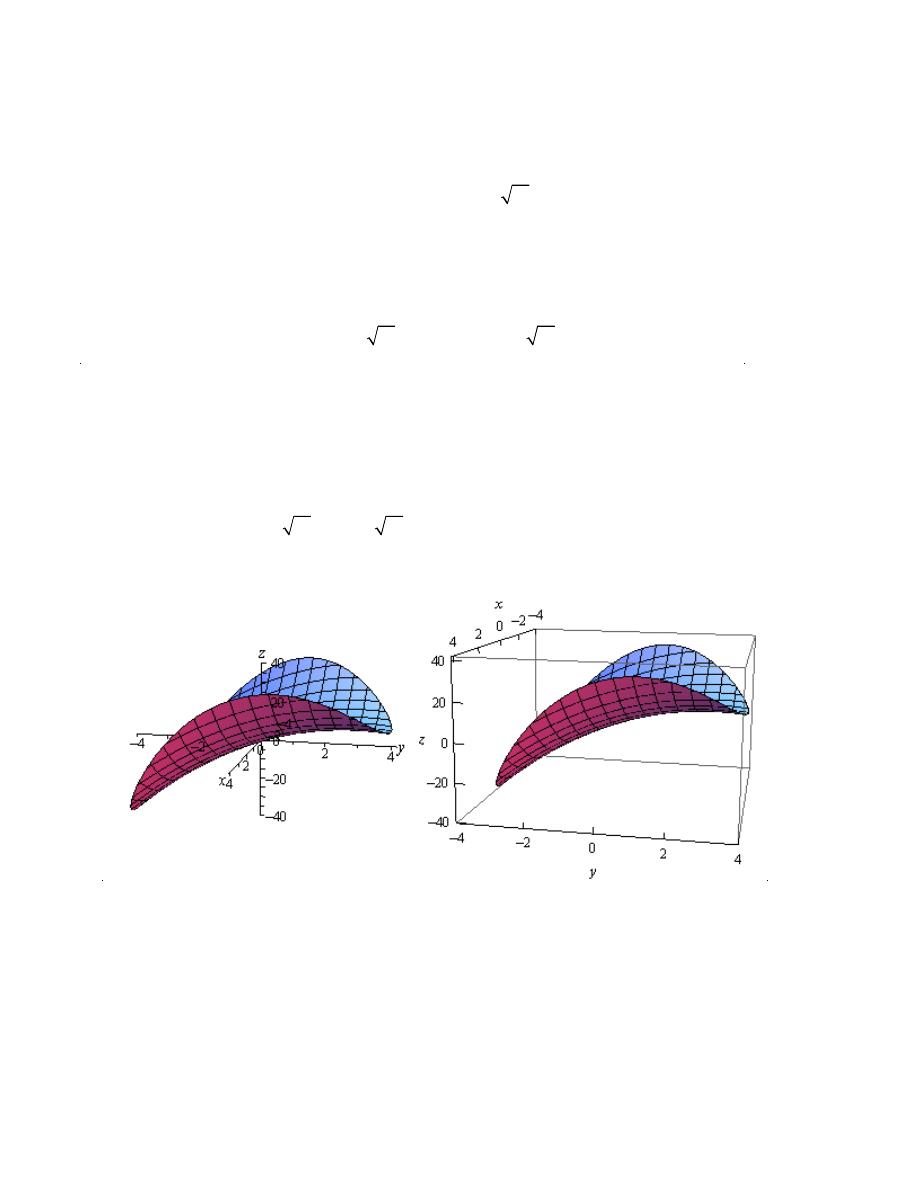
Dr.Eng Muhammad.A.R.yass
The value of this function at the critical point and the endpoints are,
( )
( )
( )
4
40
4
8
1
35
g
g
g
- = -
=
=
Unlike the first example we will still need to find the values of x that correspond to these. We
can do this by plugging the value of y into our equation for the circle and solving for y.
2
2
2
4 :
16 16 0
0
4 :
16 16 0
0
1 :
16 1 15
15
3.87
y
x
x
y
x
x
y
x
x
= -
=
-
=
Þ
=
=
=
-
=
Þ
=
=
=
- = Þ
= ±
= ±
The function values for
( )
g y
then correspond to the following function values for
( )
,
f x y
.
( )
(
)
( )
( )
( )
4
40
0, 4
40
4
8
0, 4
8
1
35
15,1
35 and
15,1
35
g
f
g
f
g
f
f
- = -
Þ
- = -
=
Þ
=
=
Þ
-
=
=
(
)
(
)
Note that the third one actually corresponded to two different values for
( )
,
f x y
since that y also
produced two different values of x.
So, comparing these values to the value of the function at the critical point of
( )
,
f x y
that we
found earlier we can see that the absolute minimum occurs at
(
)
0, 4
-
while the absolute
maximum occurs twice at
(
)
15,1
-
and
(
)
15,1
.
Here is a sketch of the region for reference purposes.
In both of these examples one of the absolute extrema actually occurred at more than one place.
Sometimes this will happen and sometimes it won’t so don’t read too much into the fact that it
happened in both examples given here.
Also note that, as we’ve seen, absolute extrema will often occur on the boundaries of these
regions, although they don’t have to occur at the boundaries. Had we given much more
complicated examples with multiple critical points we would have seen examples where the
absolute extrema occurred interior to the region and not on the boundary.
32
Dr.Eng Muhammad.A.R.yass
Small changes
If y is a function of x, i.e. y
= f (x), and the approxi-
mate change in y corresponding to a small change
δx
in x is required, then:
δy
δx
≈
dy
dx
and δy
≈
dy
dx
· δx or δy ≈ f
(x)
· δx
Example1.Given
y
= 4x
2
− x, determine the
approximate change in y if x changes from 1 to
1.02.
Since y
= 4x
2
− x, then
dy
dx
= 8x − 1
Approximate change in y,
δy
≈
dy
dx
· δx ≈ (8x − 1)δx
When x
= 1 and δx = 0.02, δy ≈ [8(1) − 1](0.02)
≈ 0.14
[Obviously, in this case, the exact value of dy
may be obtained by evaluating y when x
= 1.02,
i.e. y
= 4(1.02)
2
− 1.02 = 3.1416 and then sub-
tracting from it the value of y when x
= 1, i.e.
y
= 4(1)
2
− 1 = 3, giving δy = 3.1416 − 3 = 0.1416.
Using δy
=
dy
dx
· δx above gave 0.14, which shows
that the formula gives the approximate change in y
for a small change in x.]
Example2.The time of swing
T of a pendu-
lum is given by T
= k
√
l, where k is a constant.
Determine the percentage change in the time of
swing if the length of the pendulum l changes
from 32.1 cm to 32.0 cm.
If T
= k
√
l
= kl
1
2
, then
dT
dl
= k
1
2
l
−1
2
=
k
2
√
l
Approximate change in T ,
δt
≈
dT
dl
δl
≈
k
2
√
l
δl
≈
k
2
√
l
(
−0.1)
33
Dr.Eng Muhammad.A.R.yass
small changes
1. Determine the change in y if x changes from
2.50 to 2.51 when
(a) y
= 2x − x
2
(b) y
=
5
x
[(a)
−0.03 (b) −0.008]
2. The pressure p and volume v of a mass of
gas are related by the equation pv
= 50. If the
pressure increases from 25.0 to 25.4, deter-
mine the approximate change in the volume
of the gas. Find also the percentage change
in the volume of the gas. [
−0.032, −1.6%]
3. Determine the approximate increase in (a) the
volume, and (b) the surface area of a cube
of side x cm if x increases from 20.0 cm to
20.05 cm.
[(a) 60 cm
3
(b) 12 cm
2
]
4. The radius of a sphere decreases from 6.0 cm
to 5.96 cm. Determine the approximate
change in (a) the surface area, and (b) the
volume.
[(a)
−6.03 cm
2
(b)
−18.10 cm
3
]
5. The rate of flow of a liquid through a
tube is given by Poiseuilles’s equation as:
Q
=
pπr
4
8ηL
where Q is the rate of flow, p
is the pressure difference between the ends
of the tube, r is the radius of the tube, L
is the length of the tube and η is the coef-
ficient of viscosity of the liquid. η is obtained
by measuring Q, p, r and L. If Q can be
measured accurate to
±0.5%, p accurate to
±3%, r accurate to ±2% and L accurate
to
±1%, calculate the maximum possible
percentage error in the value of η.
[12.5%]
rates of change
1. An alternating current, i amperes, is given by
i
= 10 sin 2πft, where f is the frequency in
hertz and t the time in seconds. Determine
the rate of change of current when t
= 20 ms,
given that f
= 150 Hz.
[3000π A/s]
2. The luminous intensity, I candelas, of a lamp
is given by I
= 6 × 10
−4
V
2
, where V is
the voltage. Find (a) the rate of change of
luminous intensity with voltage when V
=
200 volts, and (b) the voltage at which the
light is increasing at a rate of 0.3 candelas
per volt.
[(a) 0.24 cd/V (b) 250 V]
3. The voltage across the plates of a capacitor at
any time t seconds is given by v
= Ve
−t/CR
,
where V , C and R are constants.
Given V
= 300 volts, C = 0.12 × 10
−6
F and
R
= 4 × 10
6
find (a) the initial rate of
change of voltage, and (b) the rate of change
of voltage after 0.5 s.
[(a)
−625V/s (b) −220.5V/s]
4. The pressure p of the atmosphere at height h
above ground level is given by p
= p
0
e
−h/c
,
where p
0
is the pressure at ground level
and c is a constant. Determine the rate
of change of pressure with height when
p
0
= 1.013 × 10
5
pascals and c
= 6.05 × 10
4
at 1450 metres.
[
−1.635 Pa/m]
tangents and normals
For the curves in problems 1 to 5, at the points
given, find (a) the equation of the tangent, and
(b) the equation of the normal.
1. y
= 2x
2
at the point (1, 2)
(a) y
= 4x − 2
(b) 4y
+ x = 9
2. y
= 3x
2
− 2x at the point (2, 8)
(a) y
= 10x − 12
(b) 10y
+ x = 82
3. y
=
x
3
2
at the point
−1, −
1
2
(a) y
=
3
2
x
+ 1
(b) 6y
+ 4x + 7 = 0
4. y
= 1 + x − x
2
at the point (
−2, −5)
(a) y
= 5x + 5
(b) 5y
+ x + 27 = 0
5. θ
=
1
t
at the point
3,
1
3
(a) 9θ
+ t = 6
(b) θ
= 9t − 26
2
3
or 3θ
= 27t − 80
Further Problem
34
Dr.Eng Muhammad.A.R.yass
maximum and minimum
9. Resistance to motion, F, of a moving vehi-
cle, is given by F
=
5
x
+ 100x. Determine the
minimum value of resistance.
[44.72]
10. An electrical voltage E is given by
E
= (15 sin 50πt + 40 cos 50πt) volts,
where t is the time in seconds. Determine
the maximum value of voltage.
[42.72 volts]
11. The fuel economy E of a car, in miles per
gallon, is given by:
E
= 21 + 2.10 × 10
−2
v
2
− 3.80 × 10
−6
v
4
where v is the speed of the car in miles per
hour.
Determine, correct to 3 significant figures,
the most economical fuel consumption, and
the speed at which it is achieved.
[50.0 miles/gallon, 52.6 miles/hour]
1. y
= 3x
2
− 4x + 2
Minimum at
2
3
,
2
3
2. x
= θ(6 − θ)
[Maximum at (3, 9)]
3. y
= 4x
3
+ 3x
2
− 60x − 12
Minimum (2,
−88);
Maximum(
− 2.5, 94.25)
4. y
= 5x − 2 ln x
[Minimum at (0.4000, 3.8326)]
5. y
= 2x − e
x
[Maximum at (0.6931,
−0.6136)]
6. y
= t
3
−
t
2
2
− 2t + 4
⎡
⎣
Minimum at (1, 2.5);
Maximum at
−
2
3
, 4
22
27
⎤
⎦
7. x
= 8t +
1
2t
2
[Minimum at (0.5, 6)]
8. Determine the maximum and minimum val-
ues on the graph y
= 12 cos θ − 5 sin θ in the
range θ
= 0 to θ = 360
◦
. Sketch the graph
over one cycle showing relevant points.
Maximum of 13 at 337
◦
23
,
Minimum of
−13 at 157
◦
23
9. Show that the curve y
=
2
3
(t
− 1)
3
+ 2t(t − 2)
has a maximum value of
2
3
and a minimum
value of
−2.
35
maximum and minimum
1. The speed, v, of a car (in m/s) is related to
time t s by the equation v
= 3 + 12t − 3t
2
.
Determine the maximum speed of the car
in km/h.
[54 km/h]
2. Determine the maximum area of a rectangu-
lar piece of land that can be enclosed by
1200 m of fencing.
[90000 m
2
]
3. A shell is fired vertically upwards and
its vertical height, x metres, is given by
x
= 24t − 3t
2
, where t is the time in seconds.
Determine the maximum height reached.
[48 m]
4. A lidless box with square ends is to be made
from a thin sheet of metal. Determine the
least area of the metal for which the volume
of the box is 3.5 m
3
.
[11.42 m
2
]
5. A closed cylindrical container has a surface
area of 400 cm
2
. Determine the dimensions
for maximum volume.
radius
= 4.607 cm;
height
= 9.212 cm
7. The power developed in a resistor R by a
battery of emf E and internal resistance r is
2
given by P
= E R
(R
+ r)
2
. Differentiate P with
respect to R and show that the power is a
maximum when R
= r.
8. Find the height and radius of a closed cylin-
der of volume 125 cm
3
which has the least
surface area.
height
= 5.42 cm;
radius
= 2.71 cm
6. Calculate the height of a cylinder of max-
imum volume which can be cut from a cone
of height 20 cm and base radius 80 cm.
[6.67 cm]