
Dr. Hussein Majeed Salih
Fluid Machinery
FLUID MACHINERY
Third Year – Power Engineering
Electromechanical Engineering Department
Lecturer
Dr. Hussein Majeed Salih

Dr. Hussein Majeed Salih
Fluid Machinery
Chapter One
Dynamic action of fluid
1. Turbo machines
Are devices in which energy is transferred either to, or from, a
continuously flowing fluid by the dynamic action of moving blades on
the runner.
Dynamic action of fluid
A stream of fluid entering in a machine such as a hydraulic or steam
turbine, a pump or fan has more or less a defined direction. A force is
always required to act upon the fluid to change its velocity either in
direction or in magnitude. Newton's Third law of motion states that to
every action there is an equal and opposite reaction. According to this
law an equal and opposite force is exerted by the fluid upon the body
that cause the change. This force exerted by virtue of fluid motion is
called a "Dynamic force".
The major problem in turbo-machinery is to find the power developed
(or consumed) by (or in) a particular machine. The power is
determined from the dynamic force or forces which are being exerted
by the following fluid on the boundaries of flow passage and which
are due to change of momentum. These are determined by applying
"Newton's Second Law of Motion".
Newton's Second Law of Motion, linear momentum equation and its
application
The fundamental principle of dynamics is Newton's Second Law of
Motion which states that " The rate of change of momentum is
proportional to the applied force and take place in the direction of the
force". More precisely this statement may be written as "The resultant
of an external force F
R
x
R
acting on the particle of mass m along any
arbitrarily chosen direction x is equal to the time rate change of linear
momentum of the particle in the same direction i.e., x-direction.
Momentum of the body is the product of its mass and velocity.
Let m be the mass of fluid moving with velocity v and let the change
of velocity be dv in time dt.
∴
change of momentum =
dv
m.

Dr. Hussein Majeed Salih
Fluid Machinery
And rate of change of momentum =
dt
dv
m.
According to the above law;
Dynamic force applied in x-direction = Rate of change of momentum
in x-direction.
i.e.,
dt
dv
m
F
x
x
.
=
For a control volume with fluid entering with uniform velocity
1
x
v
,
and leaving after time t with uniform velocity
2
x
v
, thus:
(
)
1
2
x
x
x
v
v
t
m
F
−
=
∑
i.e.,
(
)
1
2
x
x
x
v
v
Q
F
−
=
∑
ρ
Where Q is the rate of flow and
ρ
the density.
External force
x
F
may be three kinds:
1. Pressure force and those acting between the fluid and boundary
surfaces, or between any two adjacent fluid layer.
2. Inertia force : are those caused by the action of gravity and or
centrifugal effects. These are also known as " body forces".
3. Drag forces: are those existing between boundary surfaces and
flow. These are also known as " viscous forces".
There are two kinds of applications of linear-momentum equation:
1. To determine the forces exerted by the flowing fluid on the
boundaries of flow passage due to change of momentum.
2. To determine the flow characteristics when there is some loss of
known quantity of energy in the flow system such as sudden
enlargement of a pipe cross-section and hydraulic jump in an open
channel flow.
In this cores we are concerned with the applications under (1) above.
1.2
U
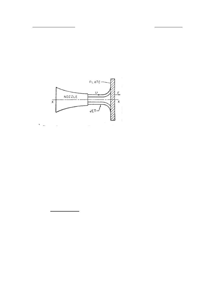
Dynamic force exerted by fluid on fixed and moving flat plates:
1.2.1
U
Plate normal to jet :
Dr. Hussein Majeed Salih
Fluid Machinery
A fluid jet issues from a nozzle and strikes a flat plate with a velocity
v. The plate is held stationary and perpendicular to the centre line of
the jet.
Applying the following equation :
(
)
1
2
x
x
x
v
v
Q
F
−
=
∑
ρ
(
)
Qv
v
Q
F
x
ρ
ρ
−
=
−
=
−
0
The minus sign on right hand side of the equation indicates that the
velocity is decreasing, while this sign used with
x
F
indicates that the
force is acting in the negative direction of x-axis.
Now the force exerted by the fluid on the plate is given by " Newton's
Law of Action and Reaction" which will be equal and opposite,
Qv
F
x
ρ
=
1.2.2
U
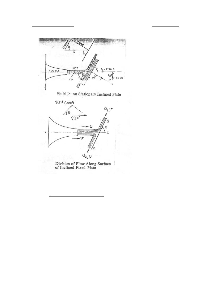
Inclined plate
The dynamic force acting normal to the plate is given by:
θ
ρ
sin
Qv
F
=
Component of this force F in the direction of jet
θ
ρ
θ
2
sin
sin
.
Qv
F
F
x
=
=

Dr. Hussein Majeed Salih
Fluid Machinery
Let
s
F
be the force along the inclined surface of plate, and Q
R
1
R
and Q
R
2
R
the quantities of flow along the surface as shown. As there is no
change in pressure elevation before and after the impact and
neglecting losses due to impact, no force is exerted on the fluid by the
plate in s-direction,
v
Q
v
Q
Qv
F
s
2
1
cos
0
ρ
ρ
θ
ρ
−
=
=
=
But
2
1
cos
Q
Q
Q
−
=
θ
From equation of continuity
2
1
Q
Q
Q
−
=
From the above two equations:
(
)
θ
cos
1
2
1
1
+
= Q
Q
and
(
)
θ
cos
1
2
1
2
−
= Q
Q
Dr. Hussein Majeed Salih
Fluid Machinery
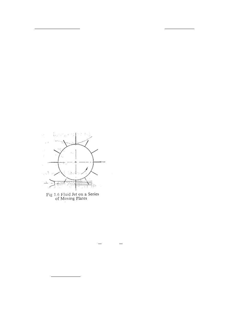
1.2.3
U
Force on moving flat plate
Let the plate in Fig.1 move with a velocity u in the same direction as
the jet, then the jet with velocity v has struck the plate. The change in
velocity is ( u-v ).
Thus
)
(
.
u
v
a
w
a
Q
−
=
=
Where
a: cross-sectional area.
w: velocity of jet relative to the motion of plate.
v: absolute velocity of jet.
∴
Force exerted on the fluid by the vane F
R
x
R
is equal:
Dr. Hussein Majeed Salih
Fluid Machinery
)
(
v
u
Q
F
x
−
=
ρ
And force exerted by the fluid on the vane is:
2
)
(
)
(
u
v
a
u
v
Q
F
x
−
=
−
=
ρ
ρ
Here the distance between plate and nozzle is constantly increasing by
u m/s. A single moving plate is, therefore, not a practical case. If,
however, a series of plates as shown in figure, were so arranged that
each plate appeared successively before the jet in the same position
always moving with a velocity u in the direction of jet, then whole
flow from the nozzle is utilized by the plates.
)
(
u
v
av
F
−
=
∴
ρ
Work done on the plates = F.u
u
u
v
Q
).
(
−
=
ρ
kinetic energy of jet
2
2
.
.
.
2
1
.
.
2
1
v
Q
v
m
ρ
=
=
Where m is the mass of fluid
∴
Efficiency of system ,
input
energy
obtaine
work
=
η

Dr. Hussein Majeed Salih
Fluid Machinery
2
2
).
(
2
.
.
2
1
).
(
.
v
u
u
v
v
Q
u
u
v
Q
−
=
−
=
ρ
ρ
For
0
max
=
⇒
du
d
η
η
(
)
0
2
0
2
=
−
⇒
=
−
∴
u
v
u
vu
du
d
2
v
u
=
∴
Substituting the value of u in equation of
η
50
5
.
0
2
).
2
(
2
2
max
or
v
v
v
v
=
−
=
η
%
1.3
U
dynamic force exerted by fluid on stationary and moving plates
1.3.1
U
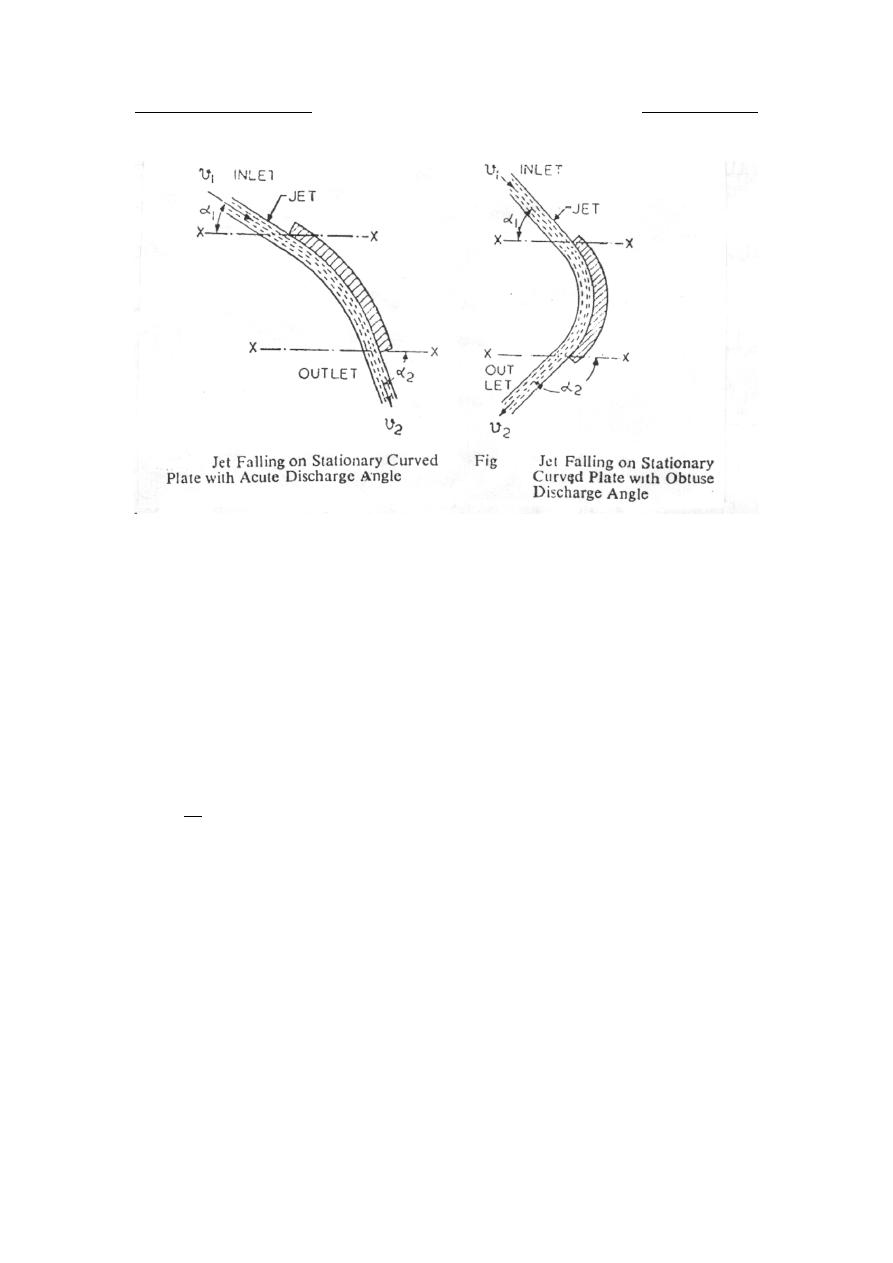
on stationary curved plates
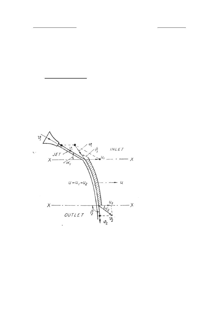
The jet impinges on a curved plate at an angle
2
1
α
α
and
at inlet and exit
respectively both angles measured with respect to x-direction, as shown
in figure:
Dr. Hussein Majeed Salih
Fluid Machinery
Let v
R
1
R
and v
R
2
R
be the velocities of jet at inlet and outlet respectively. The
velocities v
R
1
R
and v
R
2
R
will be same as long as there is no friction on the
plate.
Velocity of jet at inlet in x-direction
1
1
cos
α
v
=
Velocity of jet at outlet in x-direction
2
2
cos
α
v
=
∴
Force exerted on the jet by the plate in x-direction can be determine by
applying linear momentum equation.
*
t
m
F
x
=
change of velocity in x-direction.
(
)
1
1
2
2
cos
cos
α
α
ρ
v
v
Q
F
x
−
=
∴
And force exerted on the plate by the jet in x-direction.
(
)
2
2
1
1
cos
cos
α
α
ρ
v
v
Q
F
x
−
=
∴
Where Q=a.v
R
1
(
)
2
2
1
1
1
cos
cos
.
.
.
α
α
ρ
v
v
v
a
F
x
−
=
∴
Dr. Hussein Majeed Salih
Fluid Machinery
If the curvature of the plate at outlet is such that outlet angle
2
α
is more
than 90
P
o
P
, then the second term in the bracket i.e.,
2
2
cos
α
v
will be
negative. Hence in order to get more force, the curvature of the plate at
outlet should be with an obtuse angle
2
α
.
1.3.2
U
Single moving plate
Let the angle of curvature of the plate of inlet and outlet with the reversed
direction of motion of plate i.e., -u
R
1
R
be
2
1
β
β
and
, see figure. The plate
is moving with a velocity u in x-direction. Thus, the velocity of jet
relative to the motion of the plate is denoted by
1
w
. Its direction will
tangential to the point of inlet. Its magnitude is determined by the vector
sum of u and v
R
1
R
.
When the jet leaves the plate, its relative velocity will remain equal to w
R
1
R
provided there is no decrease in velocity due to friction on the surface of
flow. i.e., w
R
1
R
=w
R
2
R
. Now the absolute velocity of water at outlet v
R
2
R
will be
vector sum of w
R
2
R
and u.

Dr. Hussein Majeed Salih
Fluid Machinery
∴
Force exerted by the jet on the plate in x-direction or in the direction of
motion is determined by applying linear momentum equation:
*
t
m
F
x
=
change of velocity in x-direction.
(
)
2
2
1
1
cos
cos
α
α
ρ
v
v
Q
F
x
−
=
Where
(
)
u
v
a
Q
−
=
1
(
)(
)
2
2
1
1
1
cos
cos
α
α
ρ
v
v
u
v
a
F
x
−
−
=
For
0
cos
,
2
2
2
〈
〉
α
π
α
Then the second term in the bracket (
2
2
cos
α
v
) will be negative. Hence
in order to get more force, the curvature of the plate should be such that
2
α
is obtuse.
1.4
U
Absolute path of fluid through the machine.
When the jet strikes the moving plates, its position is given by full lines
as shown in figure below. As the plate moves with velocity u, it reaches
the position shown by dotted lines when the jet leaves it. Now there are
two paths traced by water jet, one over the plate surface which is relative
to the motion of plate and therefore appears to be moving with the plate;
and the other is known as absolute path which appears to be stationary
with respect to earth. To determine the absolute path of water particle,
take any six points ( 0 to 5) from inlet to outlet of the plate as shown in
figure below. Take the distances
3
0
2
0
1
0
,
,
−
−
−
w
w
w
S
S
S
, etc., along the
curved path of the plate from the point of entrance 0 to points 1,2,3,etc.
These are the distance traversed by the water particle with w, the velocity
of water relative to the motion of the plate in times t
R
1
R
, t
R
2
R
, t
R
3
R
, etc.,
respectively. Now take the distances
3
0
2
0
1
0
,
,
−
−
−
u
u
u
S
S
S
,etc., in the
horizontal direction from points 1,2,3,etc., respectively. These are the
distances traveled by the plate moving with u, its peripheral velocity, in
time t
R
1
R
, t
R
2
R
, t
R
3
R
, etc., respectively. Join the points
3
0
2
0
1
0
,
,
−
−
−
u
u
u
S
S
S
, etc.,
taken in horizontal direction with a curve which indicates the absolute
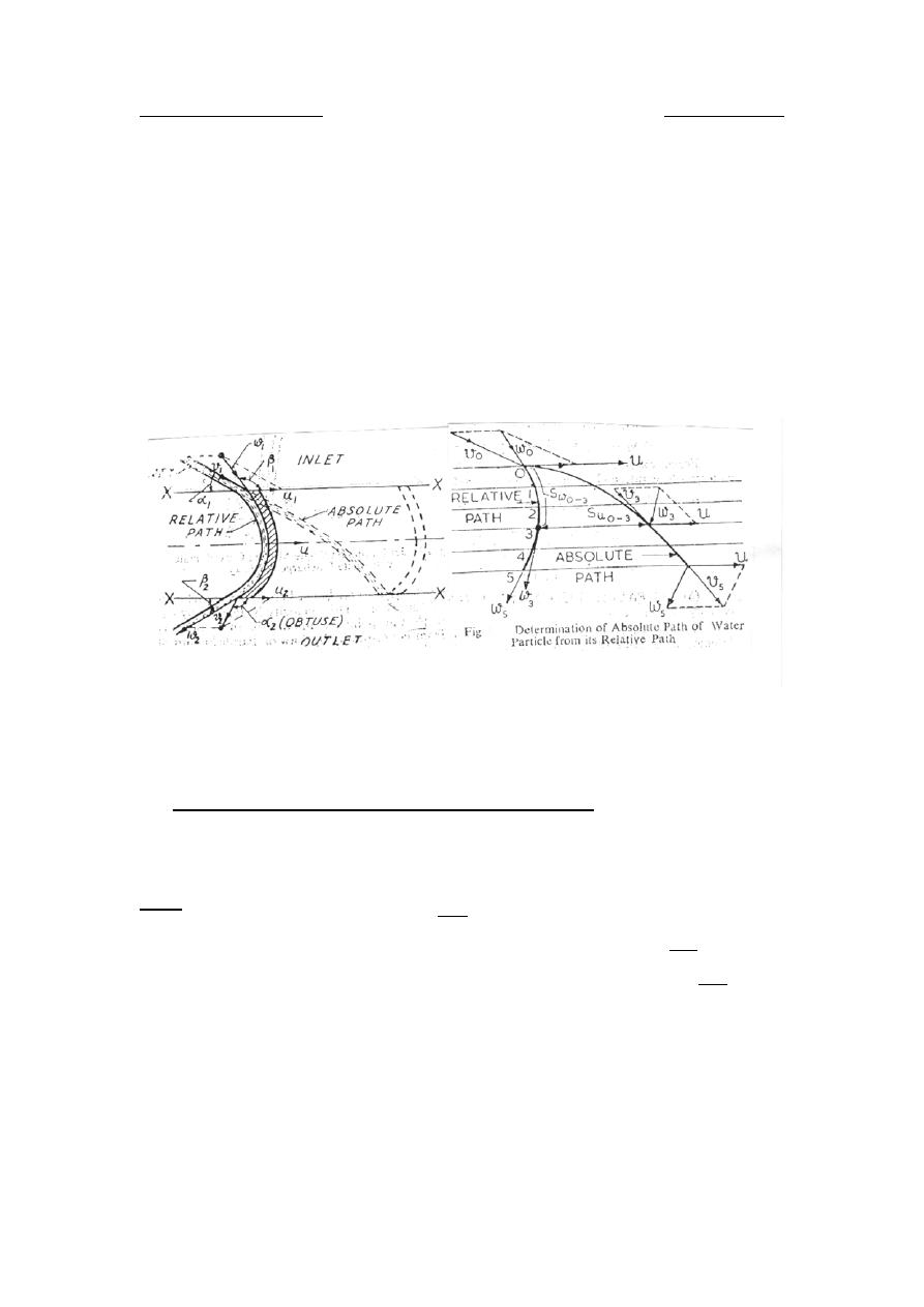
Dr. Hussein Majeed Salih
Fluid Machinery
path of water particles. The direction of absolute velocity of water at any
point will be tangential to the absolute path of water. Similarly the
direction of relative velocity of water at any point will be tangential to the
relative path of water. The direction of the peripheral velocity of plate is
always horizontal. The direction of all the three velocities u,v,w being
known. The velocity triangle can be drawn at any point of the path. The
velocity triangles have been shown at points 0, 3 and 5 in the figure.
1.5
U
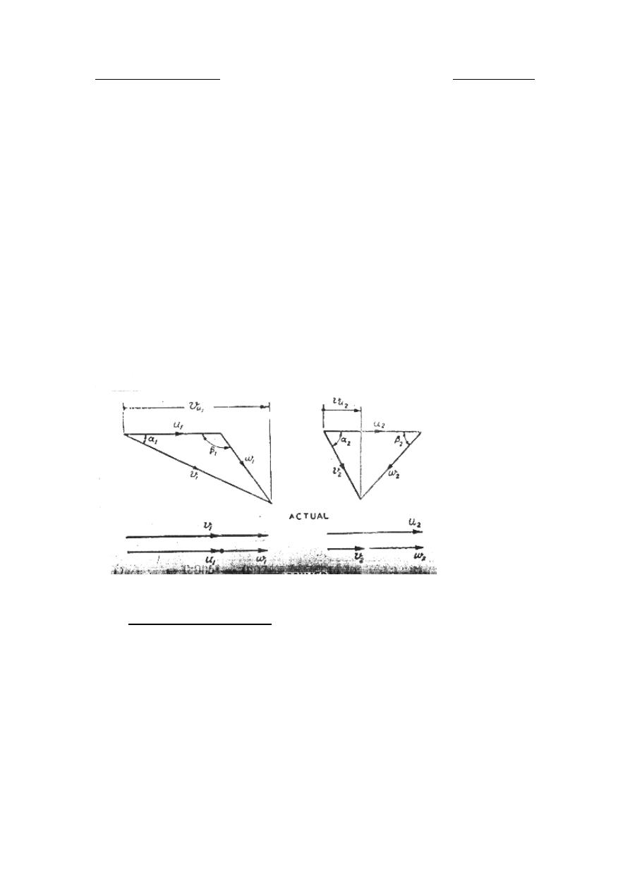
Velocity diagrams for pump and turbine blades
The velocity is a vector quantity, therefore the velocity triangle is a vector
diagram.
U
Inlet
With refer to figure below, draw
1
v
AC
= the absolute velocity of water
at inlet at an angle of
1
α
to the wheel tangent. Draw
1
u
AB
= , the
peripheral velocity of wheel in the horizontal direction. Join BC which
gives w
R
1
R
, the velocity of water relative to wheel motion at inlet, making
angle
1
β
with wheel tangent. Resolve the absolute velocity of water at
inlet into two components
1
u
v , the velocity of whirle at inlet which is the
tangent component, and
1
m
v
, the velocity of flow which is the normal
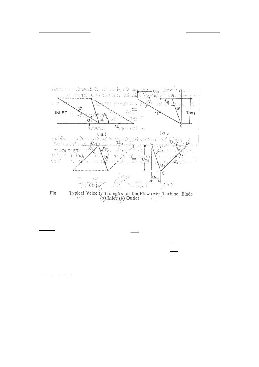
Dr. Hussein Majeed Salih
Fluid Machinery
and radial component. Mark the directions of the velocities with arrows
as shown in the figure.
U
Outlet
Refer to the previous figure. Draw
2
u
CD
=
, the peripheral velocity of
wheel at outlet in the horizontal direction. Draw
2
w
DE
=
, the relative
velocity of water at outlet at an angle
2
β
to
2
u . Join CE which gives
2
v ,
the absolute velocity of water at outlet making an angle
2
α
to the wheel
motion.
2
2
2
u
w
v
+
=
Resolve the absolute velocity of water at outlet into two components
2
2
m
u
v
and
v
, as discussed in inlet. The velocity of whirle at outlet
2
u
v
may be positive or negative, depending upon the angle
2
α
being acute or
obtuse respectively.

Dr. Hussein Majeed Salih
Fluid Machinery
Chapter Two
Unit and specific quantities
2.
U
Unit and specific quantities
The rat of flow, speed, power, etc., of hydraulic machines are all function
of the working head which is one of the most fundamental of all
quantities that go to determine the flow phenomena associated with
machines such as turbines and pumps. To facilitate correlation,
comparison and use of experimental data, these quantities are usually
reduced to unit heads and known as unit quantities e.g. unit flow, unit
speed, unit force, unit power and unit torque, etc. Thus two similar
turbines having different data can be compared by reducing the data of
both turbines under unit head.
For similar reasons it is also convenient to use some specific quantities. A
specific quantity is obtained by reducing any quantity to a value
corresponding to unit head and some unit size. The later dimension is the
inlet diameter of runner in case of reaction turbines and least jet diameter
in Pelton turbines. When two different turbines are to be compared, it can
be done by reducing their data to specific quantities.
2.1
U
Unit quantities
2.1.1
U
Unit rate of flow
Rate of flow = cross-sectional area * velocity of flow
mo
v
Q
∝
But
H
g
v
mo
mo
k
v
.
2
.
=
Where H is the head and
mo
v
k
some velocity coefficient.
H
Q
∝
∴
or
H
k
Q
1
=
∴
Now when H=1
1
1
1
1
1
Q
k
k
k
Q
=
⇒
=
=
∴
Where Q
R
1
R
is the unit rate of flow.
Dr. Hussein Majeed Salih
Fluid Machinery
∴
The unit rate of flow =
H
Q
Q
=
1
2.1.2
U
Unit speed
Let N rpm be the speed of the turbine, then linear or peripheral velocity
of runner at inlet.
60
.
.
1
1
N
D
u
π
=
Also
H
g
u
k
u
.
2
.
1
1
=
H
u
N
∝
∝
∴
1
or
H
k
N
.
2
=
Where k
R
2
R
is some coefficient.
Now, by definition, unit speed
1
2
2
2
1
1
N
k
k
k
N
=
⇒
=
=
H
N
k
N
=
=
∴
2
1
2.1.3
U
Unit power
The available power of a turbine:
H
Q
P
a
.
.
γ
=
And the developed power is :
H
Q
P
t
t
.
.
.
γ
η
=
Where
t
η
: turbine overall efficiency
In general turbine power is:
H
Q
P
.
.
∝
But
H
Q
∝
Dr. Hussein Majeed Salih
Fluid Machinery
H
H
P
.
∝
∴
or
2
3
3
.H
k
P
=
Where k
R
3
R
is some coefficient.
Now, by definition, unit power.
1
3
3
2
3
3
1
)
1
(
P
k
k
k
P
=
⇒
=
=
2
3
3
1
H
P
k
P
=
=
∴
2.1.4.
U
Unit force
The force exerted by jet on Pelton runner at its periphery is given:
(
)
2
1
u
u
v
v
Q
F
−
=
ρ
i.e.,
u
v
Q
F
.
.
∝
But
H
Q
∝
And
H
v
u
∝
H
F
∝
∴
or
H
k
F
.
4
=
Where k
R
4
R
is some coefficient.
Now, by definition, unit force.
1
4
4
4
1
)
1
(
F
k
k
k
F
=
⇒
=
=
H
F
k
F
=
=
∴
4
1
Dr. Hussein Majeed Salih
Fluid Machinery
2.1.5
U
Unit torque:
Torque or turning moment on runner = force at periphery * radius.
R
F
T
.
=
or
F
T
∝
But
H
F
∝
H
T
∝
∴
or
H
k
T
.
5
=
Where k
R
5
R
is some coefficient.
Now, by definition, unit torque.
1
5
5
5
1
)
1
(
T
k
k
k
T
=
⇒
=
=
H
T
k
T
=
=
∴
5
1
2.2
U
Specific quantities:
2.2.1
U
Specific rate of flow, or specific flow for a reaction turbine:
For a reaction turbine
(
)
mo
o
o
v
B
D
Q
.
.
.
π
=
The dimension B
R
o
R
and D
R
o
R
generally have linear relations with D
R
1
R
, the
runner diameter at inlet, and therefore, since.
H
v
mo
∝
H
D
Q
.
2
1
∝
or
H
D
k
Q
.
.
2
1
6
=
Now, by definition, specific rate of flow.
11
6
6
2
6
11
1
.
1
.
Q
k
k
k
Q
=
⇒
=
=
H
D
Q
k
Q
.
2
1
6
11
=
=
For a Pelton turbine

Dr. Hussein Majeed Salih
Fluid Machinery
1
2
1
.
.
4
v
d
Q
π
=
i.e.,
H
d
Q
.
2
1
∝
where d
R
1
R
the least diameter of water jet falling on turbine runner.
H
d
Q
Q
.
2
1
11
=
2.2.2
U
Specific power
U
Power,
H
Q
P
.
∝
Since
H
D
Q
.
2
1
∝
for a reaction turbine
2
3
2
1
. H
D
P
∝
∴
or
2
3
2
1
7
.
.
H
D
k
P
=
Now, by definition, the specific power.
11
7
7
2
3
2
7
11
)
1
.(
1
.
P
k
k
k
P
=
⇒
=
=
2
3
2
1
7
11
.H
D
P
k
P
=
=
∴
Similarly for a Pelton turbine.
2
3
2
1
11
.H
d
P
P
=
∴
Dr. Hussein Majeed Salih
Fluid Machinery
2.2.3
U
Specific force of jet on periphery of runner
(
)
2
1
u
u
v
v
Q
F
−
=
ρ
or
u
v
Q
F
.
.
∝
But
H
Q
∝
And
H
d
v
u
.
2
1
∝
and
H
v
u
∝
H
d
F
.
2
1
∝
∴
or
H
d
k
F
.
.
2
1
8
=
By definition, the specific force.
11
8
8
2
8
11
)
1
.(
1
.
F
k
k
k
F
=
⇒
=
=
H
d
F
k
F
.
2
1
8
11
=
=
∴
2.2.4
U
Specific torque
Torque = peripheral force * radius of runner.
F
T
∝
or
H
d
T
.
2
1
∝
or
H
d
k
T
.
.
2
1
9
=
by definition, the specific torque,
11
9
9
2
9
11
)
1
.(
1
.
T
k
k
k
T
=
⇒
=
=
Dr. Hussein Majeed Salih
Fluid Machinery
H
d
T
k
T
.
2
1
9
11
=
=
∴
Alternatively ,
ω
P
T
=
Where
ω
is the angular velocity
H
∝
ω
2
1
2
3
2
1
2
3
2
1
.
.
H
H
D
T
H
D
P
∝
⇒
∝
∴
or
H
D
T
.
2
1
∝
∴ specific torque
H
d
T
T
.
2
1
11
=
2.2.5
U
Specific speed of a turbine
N
D
u
.
.
1
1
π
=
and
H
u
∝
1
N
H
D
∝
∴
1
H
Q
P
t
.
∝
Where
H
D
Q
.
2
1
∝
2
3
2
1
.H
D
P
t
∝
∴
Substituting for D
R
1,
2
2
5
2
3
2
.
N
H
P
H
N
H
P
t
t
∝
⇒
∝
Dr. Hussein Majeed Salih
Fluid Machinery
or
t
P
H
N
2
5
∝
or
t
s
P
H
N
N
4
5
.
=
where
4
5
.
H
P
N
N
t
s
=
If P
R
t
R
=1 and H=1
⇒
N
R
s
R
=N
N
R
s
R
is, therefore, by definition, the specific speed of a turbine.

Dr. Hussein Majeed Salih
Fluid Machinery
Chapter Three
Hydroelectric power plants
3.1
U
Introduction
The purpose of a hydroelectric power plant is to harness power from
water flowing under pressure. As such it incorporates a number of water
driven prime-movers known as water turbines.
Water flowing under pressure has two forms of energy kinetic and
potential. The kinetic energy depends on the mass of water flowing and
its velocity while the potential energy exists as result of the difference in
water level between two points which is known as "head". The water or
hydraulic turbine, as it is sometimes named, converts the kinetic and
potential energies possessed by water into mechanical power.
3.2
U
Head and flow rate or discharge
Head is the difference in elevation between two levels of water. The head
of a hydroelectric power plant is entirely dependent on the topographical
conditions. Head can be characterized as: gross head, and net or effective
head.
3.2.1
U
Gross head
Is defined as the difference in elevation between the head race level at the
intake and the tail race level at the discharge side, naturally, both the
elevations have to be measured simultaneously. The gross head may vary
as both the elevations of water do not remain the same at all times. It is
essential to known the maximum and minimum as well as the normal
values of the gross head. The normal value would be that for which the
plant works most of the time. In rainy season the flood may raise the
elevation of tail race, thus, reducing the gross head. On the other hand at
the time of draught the same may be increased.
3.2.2
U
Net or effective head
Is the head obtained by subtracting from gross head all losses in carrying
water from the head race to the entrance of the turbine. The losses are due
to friction occurring in tunnels, canals and penstocks which lead the water
into the turbine. Net or effective head is, therefore, the true pressure
difference between the entrance to the turbine casing and the tail race
water elevation.

Dr. Hussein Majeed Salih
Fluid Machinery
3.2.3
U
Flow rate or discharge of water
It is the quantities of water used by the water turbine in unit time and is
generally measured in (m
P
3
P
/s) or ( l/s).
3.3
U
Essential components of hydroelectric power plant.
3.3.1
U
Storage reservoir
The water available from a catchment area is stored in a reservoir, so that
it can be utilized to run the turbines for producing electric power
according to the requirement through out the year. The storage reservoir
may be natural or artificial.
3.3.2
U
Dam with its control works
Dam is a structure erected on suitable site to provide for the storage of
water and to create head. Dam may be built to make an artificial reservoir
from a valley or it may be erected in a river to control the flowing water.
Structures and appliances to control the supply of water from the storage
reservoir through the dam, are known as control works or head works.
The principal elements of control works are:
a. Gates and valves.
b. Structures necessary for their operation.
c. Devices for the protection of gates and hydraulic machines, which
consist of:
i. Trashracks: They are made up of a row of rectangular cross
sectional structural steel bars placed across the intake opening is an
inclined position. They are used to obstruct debris from going into
the intake.
ii. Debris cleaning device fitted on the trashrack.
iii. Heating element against ice troubles.
3.3.3
U
Waterways with their control works.
Is a passage through which the water is carried from the storage reservoir
to the power house. It may consist of tunnels, canals, forebays and pipes (
i.e., penstocks) as shown in figure below. The control works for the
tunnels, canals, forebays and pipes may be different types of gates in
additional to these, surge tank which is reservoir fitted at some opening
made on a long pipe line to receive the rejected flow when the pipeline is
suddenly closed by a valve at its steep end. The surge tank, therefore,
Dr. Hussein Majeed Salih
Fluid Machinery
controls the pressure variations resulting from the rapid changes in
pipeline flow thus eliminating water hammer effects.
3.3.4
U
Power house
Is a building to house the turbines, generators and other accessories for
operating the machines.
3.3.5
U
Tail race
Is a waterway to conduct the water discharged from the turbines to a
suitable point where it can be safely disposed of or stored to be pumped
back into the original reservoir.
3.3.6
U
Generation and transmission of electric power
It consists of electrical generating machines, transformers, switching
equipments and transmission lines.
3.4
U
Classification of water power plants
3.4.1
U
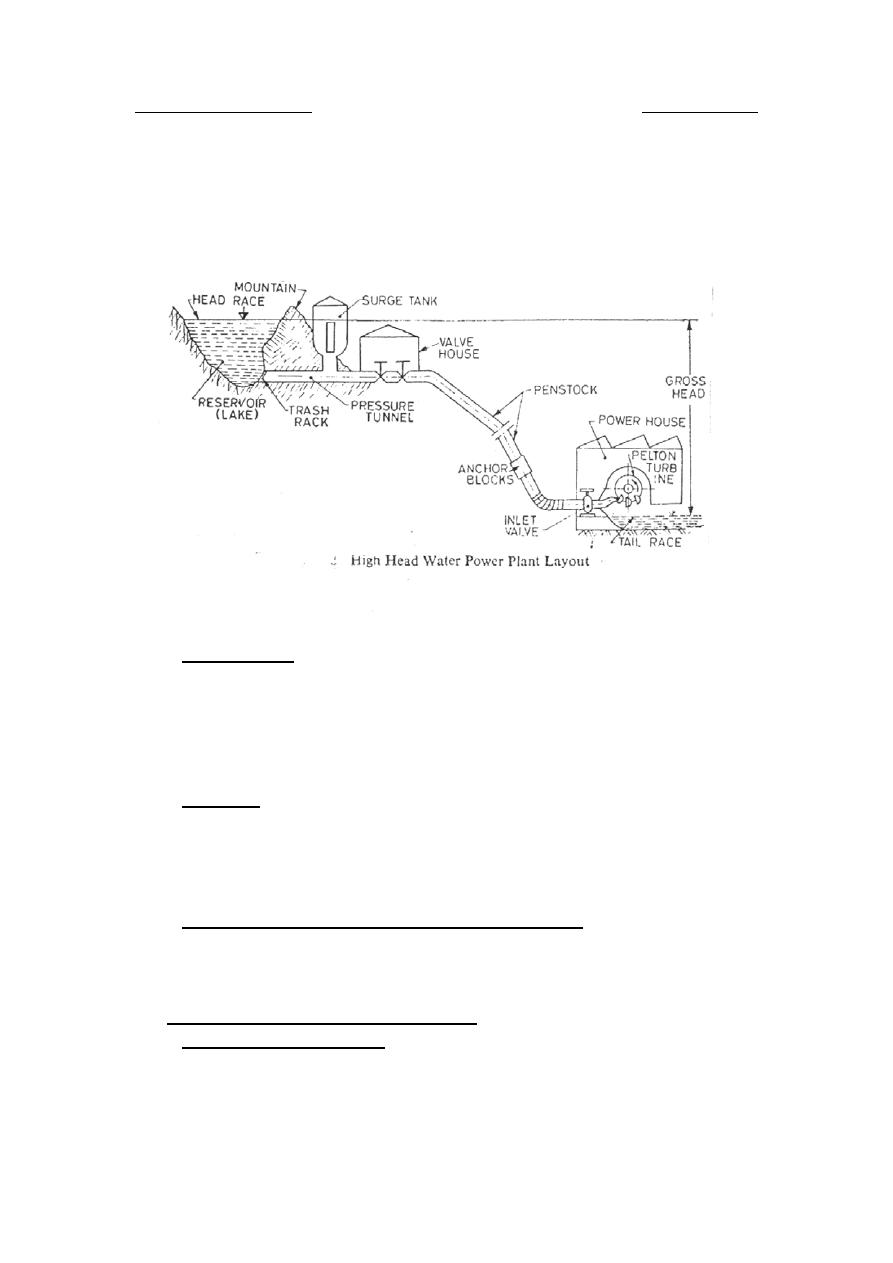
High head water plants
Such plants works under heads ranging from (25 to 2000) m. Water is
usually stored up in lakes on high mountains during the rainy season or
during the season when the snow melts. The rate of flow should be such

Dr. Hussein Majeed Salih
Fluid Machinery
that water can last through out the year. From one end of the lake, tunnels
are constructed which lead the water into smaller reservoirs known as
forebays. The forebays distribute the water to penstocks through which it
is lead to the turbines. These forebays help to regulate the demand of
water according to the load on the turbines.
3.4.2
U
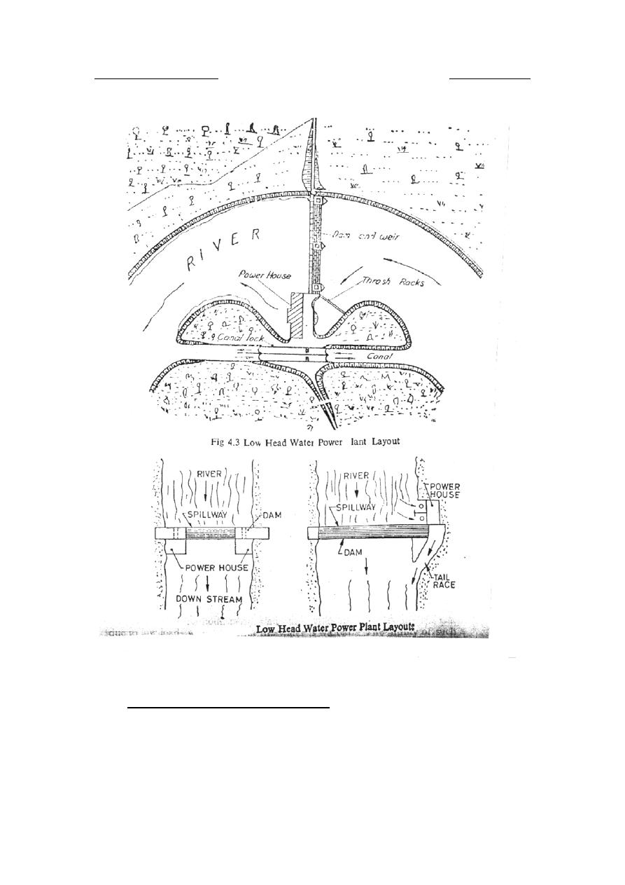
Low head water power plants
Work within the range of (25-80) m of head. These plants usually consist
of a dam across a river shown in figure below:
Dr. Hussein Majeed Salih
Fluid Machinery
3.4.3
U
Medium head water power plants
Work within (30-500) m.
It is to be noted that the above plants overlap each other. Therefore, it is
difficult to classify the plants directly on the basis of head alone. The
basis, therefore, technical adopted is the specific speed of the turbine used

Dr. Hussein Majeed Salih
Fluid Machinery
for a particular plant, as explained in the previous chapter from the above
one can classify the hydraulic turbine according to:
a. Head at the inlet of turbine
i. High head turbine (250-1800) m. Example: Pelton wheel.
ii. Medium head turbine (50-250) m. Example: Francis turbine.
iii. Low head turbine (less than 50) m. Example: Kaplan turbine.
b. Specific speed of the turbine.
i. Low specific speed turbine (
〈
50) m.
Example: Pelton wheel.
ii. Medium specific speed turbine (
250
50
〈
〈
s
N
) m.
Example: Francis turbine.
iii. Low head turbine (
〉
250) m.
Example: Kaplan turbine.

Dr. Hussein Majeed Salih
Fluid Machinery
Chapter Four
Pelton turbine or Impulse turbine
4.1
U
Introduction
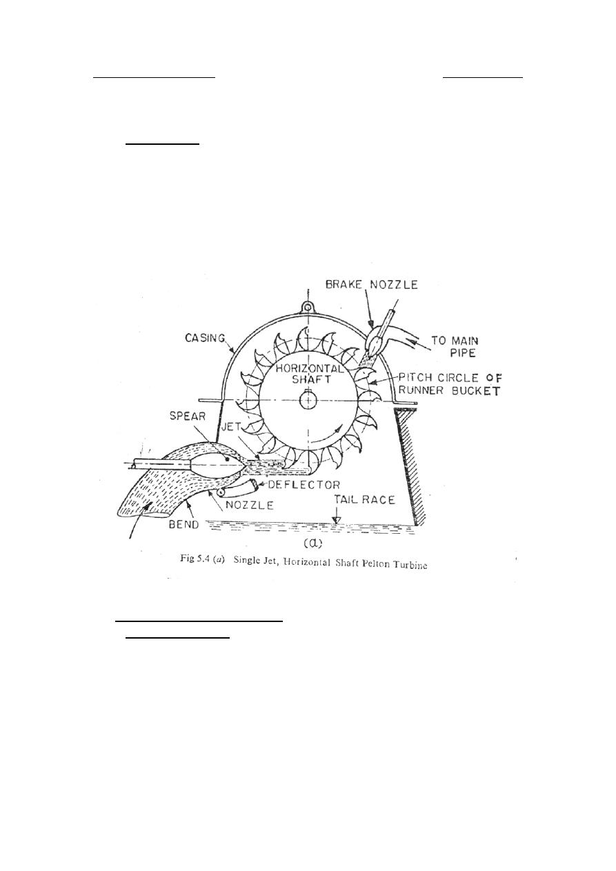
The Pelton wheel turbine is a pure impulse turbine in which a jet of fluid
leaving the nozzle strikes the buckets fixed to the periphery of a rotating
wheel. The energy available at the inlet of the turbine is only kinetic
energy. The pressure at the inlet and outlet of the turbine is atmospheric.
The turbine is used for high heads ranging from (150-2000) m. The
turbine is named after L. A. Pelton, an American engineer.
4.2
U
Parts of the Pelton turbine
4.2.1
U
Nozzle and flow control arrangement
The water from the reservoir flows through the penstocks at the outlet of
which a nozzle is fitted. The nozzle converts the total head at the inlet of
the nozzle into kinetic energy. The amount of water striking the curved
buckets of the runner is controlled by providing a spear in the nozzle. The
spear is a conical needle which is operated either by a hand wheel or
automatically in an axial direction depending upon the size of the unit.
4.2.2
U
Runner and buckets
The rotating wheel or circular disc is called the runner. On the periphery
of the runner a number of buckets evenly spaced are fixed. The shape of
the buckets is of a double hemispherical cup or bowl. Each bucket is
divided into two symmetrical parts by a dividing wall which is known as
the splitter. The jet of water strikes on the splitter. The splitter then
divides the jet into two equal parts and the water comes out at the outer
edge of the bucket. The buckets deflect the jet through an angle between
(160
P
o
P
-165
P
o
P
) in the same plane as the jet. Due to this deflection of the jet,
the momentum of the fluid is changed reacting on the buckets. A bucket
is therefore, pushed away by the jet.
4.2.3
U
Casing
The casing prevents the plashing of the water and discharges the water to
tail race. The spent water falls vertically into the lower reservoir or tail
race and the whole energy transfer from the nozzle outlet to tail race take
place at a constant pressure. The casing is made of cast iron or fabricated
steel plates.
Dr. Hussein Majeed Salih
Fluid Machinery
4.2.4
U
Breaking jet
To stop the runner within a short time, a small nozzle is provided which
directs the jet of water on to the back of the vanes. The jet of water is
called the "breaking jet ". If there is no breaking jet, the runner due to
inertia goes on revolving for a long time.
4.3
U
Force, Power and efficiency
4.3.1
U
Velocity triangles
In a Pelton wheel the jet strikes a number of buckets simultaneously. It
commences to strike the bucket before it has reached a position directly
under the centre of the wheel. The angle which the striking jet makes with
the direction of motion of the bucket is denoted by symbol
1
α
and in
practice it varies from (8
P
o
P
-20
P
o
P
). As discussed in chapter one the force
exerted by the jet can be calculated with the help of velocity triangles at
inlet and outlet.
Dr. Hussein Majeed Salih
Fluid Machinery
In drawing the typical velocity triangles for a Pelton runner, the following
points should be kept in mind:
2
1
u
u
=
since r
R
1
R
=r
R
2
2
1
w
w
=
assuming there is no friction at the blades
1
1
β
α
〈
2
1
v
v
〉〉〉
1
2
α
α
〉
1
1
v
u
〈
2
2
w
v
〈
4.3.2
U
Force exerted by the jet
For the calculation of the force exerted by the jet, it is assumed that
0
1
=
α
i.e., the bucket face is perpendicular to the jet.
If
0
1
=
α
,
o
180
1
=
β
Then
1
1
1
1
1
1
cos
w
u
v
v
v
u
+
=
=
=
α
or
1
1
1
u
v
w
−
=

Dr. Hussein Majeed Salih
Fluid Machinery
From velocity triangle at outlet
2
2
2
2
2
2
cos
cos
β
α
w
u
v
v
u
−
=
=
For ideal case
0
2
=
β
i.e., water is deflected back by 180
P
o
2
2
2
w
u
v
u
−
=
∴
)
1
0
(cos
=
But
2
1
u
u
=
and
2
1
w
w
=
1
1
2
w
u
v
u
−
=
∴
(
)
1
1
1
1
1
2
v
u
u
v
u
−
=
−
−
=
Force exerted by the jet in the direction of u
R
1
(
)
2
1
u
u
u
v
v
Q
F
−
=
ρ
Assuming that the total quantity of Q strikes the bucket.
or
(
)
[
]
1
1
1
2
v
u
v
Q
F
u
−
−
=
ρ
(
)
1
1
2
u
v
Q
−
=
ρ
Also
gH
k
d
Q
v
2
.
.
.
4
1
2
1
π
=
gH
k
v
v
2
.
1
1
=
,
gH
k
u
u
2
.
1
1
=
Substituting these values in F
R
u

Dr. Hussein Majeed Salih
Fluid Machinery
(
)
gH
k
k
qH
k
d
F
u
v
v
u
2
2
.
.
4
2
1
1
1
2
1
−
=
π
ρ
(
)
H
g
d
k
k
k
u
v
v
.
.
.
.
2
1
1
1
1
−
=
ρπ
(
)
H
d
k
k
k
u
v
v
.
.
.
2
1
1
1
1
−
=
γπ
Hence, force for unit head and unit diameter
(
)
γ
π
.
.
1
1
1
11
u
v
v
u
k
k
k
F
−
=
Per unit head and unit jet diameter.
Force will be maximum when
0
1
=
u
k
, i.e., wheel is at rest.
(
)
γ
π
.
.
2
1
max
11
v
u
k
F
=
Substituting average values
985
.
0
1
=
u
k
and
3
9800
m
N
=
γ
(
)
(
)
kN
F
u
87
.
29
9800
*
985
.
0
.
2
max
11
=
=
π
Per unit head and unit jet diameter.
Under normal working conditions
45
.
0
1
≅
u
k
(
)
kN
F
u
22
.
16
9800
*
45
.
0
985
.
0
985
.
0
*
11
=
−
=
∴
π
For running speed ( i.e., speed at no load or in other words, the vanes or
wheel running away from the jet with the same velocity as that of the jet.
1
1
v
u
k
k
=
∴
Then
0
11
=
u
F
Theoretically for maximum efficiency
2
1
1
=
u
v
k
k
Dr. Hussein Majeed Salih
Fluid Machinery
This can be proved as follows:
Power
(
)
1
1
1
1
.
2
.
u
u
v
Q
u
F
P
u
−
=
=
ρ
For given
1
v
, the power attains maximum value when:
(
)
0
2
2
1
1
1
=
−
=
u
v
Q
du
dP
ρ
or
1
1
2u
v
=
or
2
1
1
=
u
v
but in practice, on account of losses
8
.
1
1
1
=
u
v
k
k
4.3.3
U
Work done and power developed by the jet
u
F
P
u
H
.
=
(kW)
gH
k
H
d
k
k
k
u
u
v
v
2
.
.
).
.(
.
.
1
2
1
1
1
1
−
=
π
γ
Power developed per unit head and unit jet diameter:
g
k
k
k
k
H
d
P
P
u
v
u
v
H
H
2
).
.(
.
.
.
.
1
1
1
1
2
3
2
1
11
−
=
=
π
γ
Substituting average values
985
.
0
1
=
v
k
and
45
.
0
1
=
u
k
32
.
32
11
=
H
P
kW per unit head and unit jet diameter.
Dr. Hussein Majeed Salih
Fluid Machinery
4.3.4
U
Turbine efficiency
4.3.4.1
U
Jet efficiency or head efficiency
Head efficiency
)
.(
.
4
.
2
.
.
4
.
2
.
.
).
.(
.
.
1
1
1
1
2
1
1
2
1
1
1
1
u
v
u
v
u
u
v
v
a
H
H
k
k
k
H
gH
k
d
gH
k
H
d
k
k
k
P
P
−
=
−
=
=
π
γ
π
γ
η
For maximum efficiency, assuming
1
v
k
as constant,
0
1
=
u
H
dk
d
η
or
0
)
2
.(
4
1
1
=
−
u
v
k
k
2
2
1
1
1
1
v
u
k
k
v
u
=
⇒
=
∴
( )
2
1
1
1
1
max
2
.
2
.
4
v
v
v
v
H
k
k
k
k
=
−
=
∴
η
Taking the average value of
985
.
0
1
=
v
k
( )
97
.
0
985
.
0
2
max
=
=
∴
H
η
In the ideal case
( )
1
max
=
H
η
but actually it is within 0.96 to 0.98.
4.3.4.2
U
Volumetric efficiency
The total quantity of water contained in the jet does not strike the bucket
and always there is some amount of water slips and falls in the tail race
without doing any useful work. Thus, a new factor called volumetric
efficiency is introduced.

Dr. Hussein Majeed Salih
Fluid Machinery
If
Q
∆
be the quantity of water lost on account of slip.
Q
Q
Q
Q
∆
−
=
η
Actual value of
Q
η
is between 0.97 and 0.99.
4.3.4.3
U
Hydraulic efficiency
Considering the hydraulic losses of the turbine, the hydraulic efficiency
can be written as:
Q
H
h
Q
Q
Q
H
H
H
η
η
η
.
=
∆
−
∆
−
=
4.3.4.4
U
Mechanical efficiency
There are always some mechanical losses in the transmission of power by
the turbine,
99
.
0
97
.
0
−
=
m
η
.
4.3.4.5
U
Final power output from turbines.
If
a
P
be the natural available power produced by jet,
H
a
H
P
P
η
.
=
Hydraulic power generated by turbines:
Q
H
a
Q
H
h
P
P
P
η
η
η
.
.
.
=
=
Net brake power developed by the turbine shaft,
mech
Q
H
a
mech
h
t
P
P
P
η
η
η
η
.
.
.
.
=
=
Hence, final or overall efficiency of the turbine:
mech
Q
H
a
mech
Q
H
a
a
t
t
P
P
P
P
η
η
η
η
η
η
η
.
.
.
.
.
=
=
=

Dr. Hussein Majeed Salih
Fluid Machinery
Now, it must be remember that in calculating the above values of force,
power and efficiencies it was presumed that:
2
1
2
1
0
,
180
w
w
and
o
o
=
=
=
β
β
In practice,
1
2
2
1
)
98
.
0
96
.
0
(
)
20
10
(
,
)
110
95
(
w
of
w
and
o
o
−
=
−
=
−
=
β
β
More accurate calculations for force, power and efficiencies can be made
by taking into account these facts and making the necessary corrections.

Dr. Hussein Majeed Salih
Fluid Machinery
Chapter Five
Reaction turbine ( Francis and Kaplan)
5.1
U
Francis turbine
5.1.1
U
Main components
• Penstock
Penstock is a waterway to carry water from the reservoir to the turbine
casing. Trashracks are provided at the inlet of penstock in order to
obstruct the debris entering in it.
• Casing
The water from penstocks enter the casing which is of spiral shape. In
order to distribute the water around the guide ring evenly, the area of
cross section of the casing goes on decreasing gradually. The casing is
usually made of concrete, cast steel or plate steel.
• Guide vanes
The stationary guide vanes are fixed on stationary circular wheel
which surrounds the runner. The guide vanes allow the water to strike
the vanes fixed on the runner without shock at the inlet. This fixed
guide vanes are followed by adjustable guide vanes. The cross
sectional area between the adjustable vanes can be varied for flow
control at part load.
• Runner
It is circular wheel on which a series of radial curved vanes are fixed.
The water passes into the rotor where it moves radially through the
rotor vanes and leaves the rotor blades at a smaller diameter. Later, the
water turns through 90
P
o
P
into the draft tube.
• Draft tube
• The pressure at the exit of the rotor of a reaction turbine is
generally less than the atmospheric pressure. The water at exit can
not be directly discharged to the tail race. A tube or pipe of
gradually increasing area is used for discharging the water from the
turbine exit to the tail race. In other words, the draft tube is a tube
of increasing cross sectional area which converts the kinetic energy
of water at the turbine exit into pressure energy.
Dr. Hussein Majeed Salih
Fluid Machinery
5.1.2.
U
Force, power and efficiencies
5.1.2.1
U
Force and torque
The resultant dynamic force exerted by the water on the runner vanes in
the direction of rotation.
(
)
2
1
.
u
u
u
v
v
Q
F
−
=
ρ
Force equivalent of motion at inlet
1
1
.
.
u
u
v
Q
F
ρ
=
≡
Force equivalent of motion at outlet
2
2
.
.
u
u
v
Q
F
ρ
=
≡
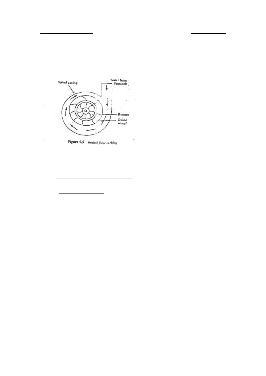
The action of the stream on the vanes of a radial flow runner can be
determined by finding the total torque produced by all elementary forces
over the vanes. The runner is considered to be divided into a number of
parts of equal area, each constituting what may be called a functional
turbine.
Let
H
dM
be the turbine moment of a functional turbine and
dQ
the
quantity of water flowing through it.
Equivalent turning moment of fluid motion at inlet :
1
1
1
1
1
.
.
.
.
R
v
dQ
R
dF
dM
u
u
H
ρ
=
=

Dr. Hussein Majeed Salih
Fluid Machinery
Similarly equivalent turning moment at outlet:
2
2
2
2
2
.
.
.
.
R
v
dQ
R
dF
dM
u
u
H
ρ
=
=
Resultant torque:
(
)
2
2
1
1
2
1
.
.
.
R
v
R
v
dQ
dM
dM
dM
u
u
H
H
H
−
=
−
=
ρ
(
)
dQ
R
v
R
v
dM
M
Q
u
u
H
H
.
.
.
0
2
2
1
1
∫
∫
−
=
=
∴
ρ
(
)
2
2
1
1
.
.
.
.
R
v
R
v
Q
M
u
u
H
−
=
∴
ρ
5.1.2.2
U
Power
Let
H
P
be the power developed by the turbine.
Then the power of a functional turbine:
ω
.
H
H
dM
dP
=
(
)
ω
ω
ρ
.
.
.
.
.
.
2
2
1
1
R
v
R
v
dQ
u
u
−
=
(
)
2
2
1
1
.
.
.
.
u
v
u
v
dQ
u
u
−
=
ρ
(
)
dQ
u
v
u
v
dP
P
Q
u
u
H
H
.
.
.
0
2
2
1
1
∫
∫
−
=
=
∴
ρ
(
)
2
2
1
1
.
.
.
.
u
v
u
v
Q
P
u
u
H
−
=
∴
ρ
5.1.3
U
Efficiency
•
U
Head efficiency
Let the total head loss in turbine be
H
∆
and the net operating head H.
Dr. Hussein Majeed Salih
Fluid Machinery
Then efficiency,
H
H
H
H
H
H
∆
−
=
∆
−
=
1
η
This is known as the "Head efficiency"
But
H
H
a
H
H
Q
P
P
η
γ
η
.
.
.
.
=
=
(
)
H
u
u
H
Q
u
v
u
v
Q
η
γ
ρ
.
.
.
.
.
.
.
2
2
1
1
=
−
∴
or
(
)
H
g
u
v
u
v
u
u
H
.
.
.
2
2
1
1
−
=
η
(
)
H
g
u
v
u
v
u
u
.
2
.
.
2
2
2
1
1
−
=
Substituting
gH
k
v
u
v
u
2
.
1
1
=
gH
k
v
u
v
u
2
.
2
2
=
gH
k
u
u
2
.
1
1
=
gH
k
u
u
2
.
2
2
=
(
)
2
1
.
.
2
2
1
u
v
u
v
H
k
k
k
k
u
u
−
=
∴
η
but
1
1
2
2
u
R
R
u
=
( since
2
2
1
1
R
u
R
u =
=
ω
)
1
2
.
1
2
u
u
k
R
R
k
=
−
=
∴
1
2
2
1
1
.
.
2
u
u
v
v
u
H
k
k
k
k
k
u
u
η

Dr. Hussein Majeed Salih
Fluid Machinery
−
=
1
2
.
.
2
2
1
1
R
R
k
k
k
u
u
v
v
u
If the discharge in radial, i.e.,
2
2
π
α
=
Then,
0
cos
2
=
α
, and
0
2
=
u
v
k
1
.
2
1
u
v
u
H
k
k
=
∴
η
•
U
Volumetric efficiency
Let
Q
∆
be the amount of water that passes over to the tail race
through some passage.
l
u
Q
Q
Q
∆
+
∆
=
∆
where
u
Q
∆
: upper clearance loss
l
Q
∆
: lower clearance loss
Volumetric efficiency
Q
Q
Q
Q
Q
Q
∆
−
=
∆
−
=
1
η
•
U
Hydraulic efficiency
Total hydraulic loss in turbine is made up of total head loss and
volumetric loss. The actual hydraulic power of the turbine is obtained
by considering the total loss.
Thus,
(
)(
)
H
H
Q
Q
P
h
∆
−
∆
−
=
γ
and
H
Q
P
a
.
.
γ
=
Hydraulic efficiency
(
)(
)
H
Q
H
H
Q
Q
P
P
a
h
h
.
.
γ
γ
η
∆
−
∆
−
=
=

Dr. Hussein Majeed Salih
Fluid Machinery
=
∆
−
∆
−
H
H
Q
Q
1
1
H
Q
h
η
η
η
.
=
•
U
Mechanical efficiency
Brake power of a turbine is the hydraulic power minus the mechanical
losses.
.
mech
h
t
P
P
P
∆
−
=
Mechanical loss may be due to bearing friction and winding.
Now, mechanical efficiency:
h
mech
h
mech
h
mech
P
P
P
P
P
.
.
.
1
∆
−
=
∆
−
=
η
∴ Brake power
.
.
mech
h
t
P
P
η
=
•
U
Overall efficiency
Let
t
η
be the overall efficiency of the turbine, then:
a
mech
h
a
t
t
P
P
P
P
.
.
η
η
=
=
.
.
.
.
.
.
.
mech
H
Q
a
mech
H
Q
a
P
P
η
η
η
η
η
η
=
=
5.1.4
U
Discharge through Francis turbine
Q=area across flow * velocity of flow
Area across radial flow at inlet
(
)
o
B
t
z
D
.
2
1
−
=
π
Dr. Hussein Majeed Salih
Fluid Machinery
where D
R
1
R
: the inlet diameter of runner.
z
R
2
R
: the number of blades in runner.
t : the thickness of blades.
B
R
o
R
: the height of runner
≅
height of guide vanes.
Radial velocity of flow at inlet:
1
1
1
sin
.
α
v
v
m
=
(
)
1
2
1
.
.
m
o
v
B
t
z
D
Q
−
=
∴
π
Now the area occupied by blade edges is usually 5 to 10 % of
1
D
π
.
In general,
(
)
1
2
1
.
. D
k
t
z
D
π
π
=
−
where k = percentage of net flow area ( 0.9 – 0.95 )
also B
R
o
R
is proportional to D
R
1
R
let
1
1
.D
k
B
k
D
B
B
o
B
o
=
⇒
=
and
gH
k
v
m
v
m
2
.
1
1
=
gH
D
k
k
k
Q
mi
v
B
2
.
.
.
.
.
2
1
π
=
∴
The factor
(
)
g
k
k
k
mi
v
B
2
.
.
.
.
π
which is constant for geometrically similar
turbines is called specific flow and is denoted by
11
Q .
Then,
H
D
Q
Q
.
.
2
1
11
=
11
Q
is therefore, the quantity of water required by the turbine when
working under unit head and with unit runner inlet diameter
( )
1
D .
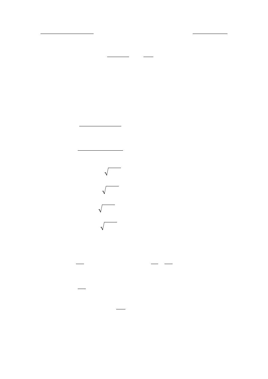
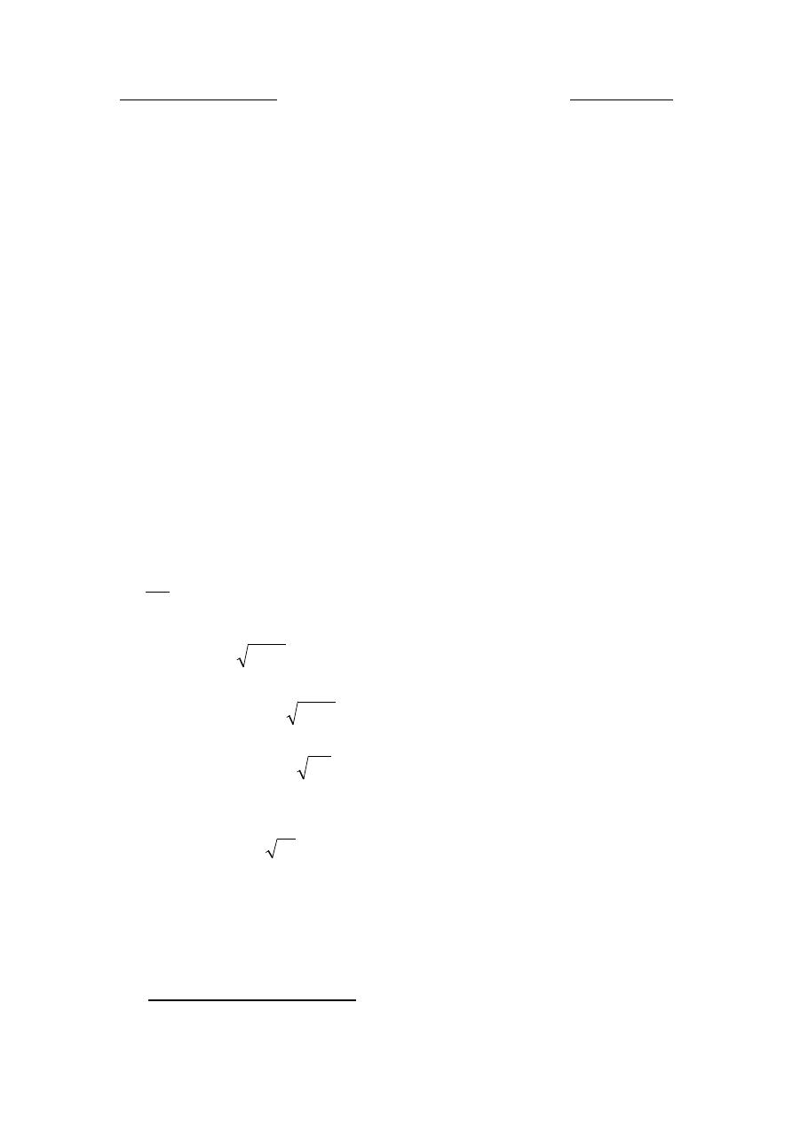
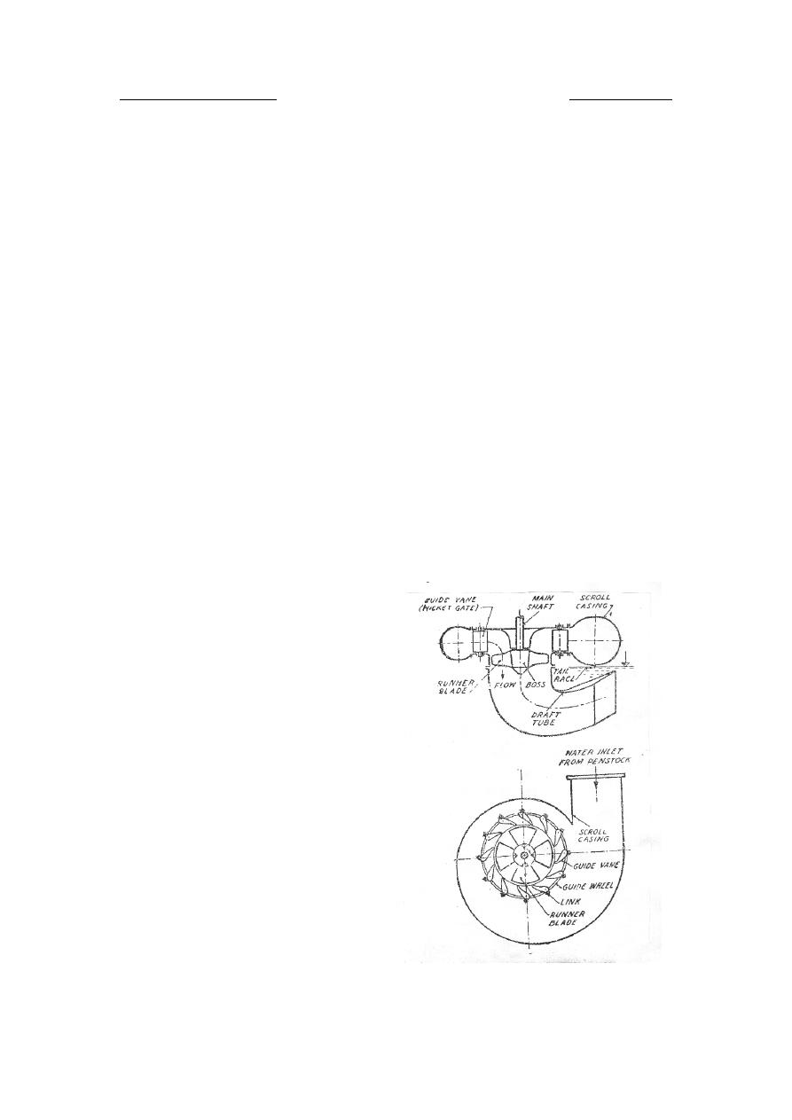
5.2
U
Axial flow reaction turbine
Dr. Hussein Majeed Salih
Fluid Machinery
In axial flow reaction turbine, water flows parallel to the axis of rotation
of the shaft. In a reaction turbine, the head at the inlet of the turbine is the
sum of pressure energy and kinetic energy and a part of the pressure
energy is converted into kinetic energy as the water flows the runner. For
the axial flow reaction turbine, the shaft of the turbine is vertical. The
lower end of the shaft which is made larger is known as "hub" or "boss".
The vanes are fixed on the hub and hence the hub acts as a runner for the
axial flow reaction turbine. The two important axial flow turbine are:
• Propeller turbine.
• Kaplan turbine.
The vanes are fixed to the hub and are not adjustable, then the turbine is
known as propeller turbine, on the other hand if the vanes on the hubare
adjustable, the turbine is known as Kaplan turbine. It is named after V.
Kaplan, an Austrian engineer. Kaplan turbine is suitable where a large
quantity of water at low heads ( up to 400 m ) is available.
The main parts of Kaplan turbine are:
• Scroll casing.
• Guide vanes.
• Hub with vanes.
• Draft tube.
Dr. Hussein Majeed Salih
Fluid Machinery
Dr. Hussein Majeed Salih
Fluid Machinery
5.2.1
U
Force, torque, power and efficiency
For the calculations of force, torque, power and various efficiencies, the
formulae derived for Francis turbine, will hold good for propeller or
Kaplan turbine also.
5.2.2
U
Rate of flow through propeller or Kaplan runner
Q= area across flow * velocity of flow.
Area across flow=
(
)
2
1
2
1
4
d
D
k
−
π
Where k : percentage of net flow area obtained after deducting area
occupied by the blades.
D
R
1
R
=D
R
2
R
: the external diameter of the runner.
d
R
1
R
: the diameter of the runner boss or hub.
Velocity of flow
gH
k
v
vm
m
2
1
1
=
(
)
H
d
D
g
k
k
Q
vm
.
.
2
.
.
.
4
2
1
2
1
1
−
=
∴
π
or
(
)
H
d
D
Q
Q
.
.
2
1
2
1
11
−
=
where
g
k
k
Q
vm
2
.
.
.
4
1
11
π
=
11
Q is a factor, constant for geometrically similar turbines (specific
flow). Its value from 0.6 to 2.175 depending upon
s
N .

Dr. Hussein Majeed Salih
Fluid Machinery
Chapter Six
Pumps
6.1
U
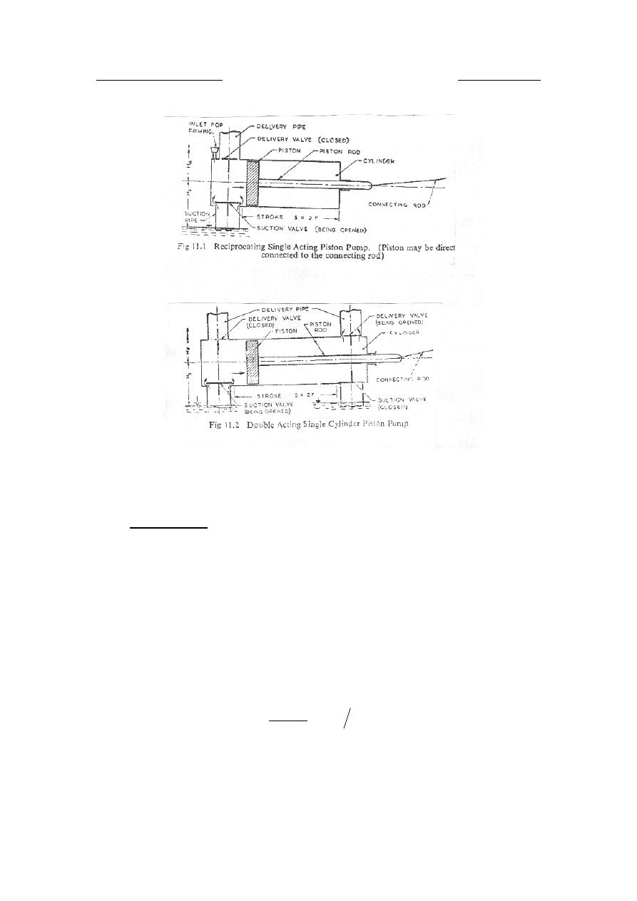
Reciprocating pumps, definition and working principle
The reciprocating pump is a positive acting type which means it is a
displacement pump which creates lift and pressure by displacing liquid
with a moving member or piston. A reciprocating pump consists
primarily of a piston or plunger reciprocating inside a close fitting
cylinder, thus performing the suction and delivery strokes. The chamber
or cylinder is alternately filled and emptied by forcing and drawing the
liquid by mechanical motion. Suction and delivery pipes are connected to
the cylinder. Each of the two pipes is provided with a non-return valve.
The function of the non-return or one way valve is to ensure
unidirectional flow of liquid. Thus the suction pipe valve allows the
liquid only to enter the cylinder while the delivery pipe valve permits
only its discharge from the cylinder. Volume or capacity delivered is
constant regardless of pressure, and is varied only by speed changes. If H
R
s
R
and H
R
d
R
be the suction and delivery heads respectively of the pump, then
(
)
d
s
H
H
H
+
=
is known as its "static head".
6.1.1
U
Applications
Reciprocating pump generally operates at low speeds and is therefore to
be coupled to an electric motor with V-belt. It is best suited for relatively
small capacities and high heads.
Dr. Hussein Majeed Salih
Fluid Machinery
6.1.2
U
Piston pump
a) Single acting
It consists of one suction and one delivery pipe simply connected to one
cylinder as shown in the previous figure, let:
A: the cross sectional area of the piston in m
P
2
P
.
a: the cross sectional area of the piston rod in m
P
2
P
.
S: the stroke of the piston in m.
N: the speed of crank in rpm.
Then, average rate of flow=
( )
s
m
N
S
A
3
60
.
.
.
Force on piston forward stroke=
A
H
s
.
.
γ
(kN).
Force on piston backward stroke=
A
H
d
.
.
γ
(kN).
Neglecting head losses in transmission and at values, power of the pump.

Dr. Hussein Majeed Salih
Fluid Machinery
(
)
)
(
60
).
.
.
.(
.
.
kW
H
H
N
S
A
H
Q
d
s
+
=
=
γ
γ
b) Double acting single cylinder pump.
It has two suction and two delivery pipes connected to one cylinder.
60
.
).
(
60
.
.
N
S
a
A
N
S
A
Q
−
+
=
60
.
.
2
60
)
2
.(
.
N
S
A
a
A
N
S
≅
−
=
( m
P
3
P
/s)
Force acting on piston in forward stroke:
)
.(
.
.
.
a
A
H
A
H
d
s
−
+
=
γ
γ
(kN)
Force acting on piston during backward stroke:
A
H
a
A
H
d
s
.
.
)
.(
.
γ
γ
+
−
=
(kN)
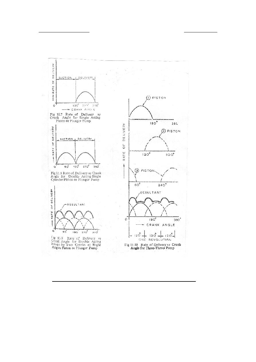
c) Two-throw pump.
It has two cylinders each equipped with one suction and one delivery
pipe. The pistons reciprocating in the cylinders are moved with the help
of connecting rods fitted with a crank at 180
P
o
P
.
60
.
.
2
N
S
A
Q
=
(m
P
3
P
/s)
d) Three-throw pump.
It has three cylinders and three pistons working with three connecting
rods fitted with a crank at 120
P
o
P
.

Dr. Hussein Majeed Salih
Fluid Machinery
60
.
.
3
N
S
A
Q
=
(m
P
3
P
/s)
6.1.3
U
Rate of delivery
The reciprocating pumps are run by crank and connecting rod mechanism
which gives the motion of piston as simple harmonic. In simple harmonic
motion (SHM) the velocity of piston is equal to
θ
ω
sin
r
.
The rate of delivery= cross sectional area of the pipe * velocity of water.
The velocity of water in the pipe
a
A
r
.
sin
.
.
θ
ω
=
Where A: cross sectional area of the piston.
a : cross sectional area of the pipe.
Thus, the rate of delivery into or out of the pump varies as
θ
sin
and it is
therefore not uniform.
Dr. Hussein Majeed Salih
Fluid Machinery
6.1.4
U
Velocity and acceleration of water in reciprocating pumps
If at any instant separation takes place (discontinuity of flow), it will
result in a sudden change of momentum of the moving water. This causes
an impulsive force which is responsible for phenomenon of "water
hummer" in reciprocating pump causes heavy shocks. As a result of this,
pump may be fracture. To eliminate this, driving force must be sufficient

Dr. Hussein Majeed Salih
Fluid Machinery
to accelerate the mass of water following the piston at the same rate as the
piston itself. Assuming that the pressure inside the cylinder is zero when
the piston moves forward, total suction pressure is equal to atmospheric
pressure and it has to work against the following forces:
• Work against gravity equivalent to suction height H
R
s
R
.
• Work against inertial force equivalent to head H
R
as
R
.
• Work against frictional forces equivalent to head H
R
f
R
.
• Work against force required to open the non-return valve
equivalent to head H
R
vs
R
.
• Work against friction in the valve equivalent to head H
R
vfs
R
.
• Work against kinetic head due to velocity of water in the suction
pipe equivalent to head
g
v
s
2
2
.
• Work against vapor pressure equivalent to head H
R
vap
R
.
vap
s
vfs
vs
fs
as
s
atm
H
g
v
H
H
H
H
H
H
+
+
+
+
+
+
=
∴
2
2
Now, let:
:
p
f
the acceleration of piston.
A : the cross-sectional area of piston.
a
R
s
R
: the cross-sectional area of suction pipe.
Then acceleration of water in suction pipe.
s
p
s
a
A
f
f
.
=
Acceleration force= mass * acceleration
s
s
s
as
f
L
a
F
.
.
.
ρ
=
( kN)
Where L
R
s
R
: the length of suction pipe.
Force per unit cross-sectional area
s
s
as
f
L
f
.
.
ρ
=
(kN/m
P
2
P
)
Dr. Hussein Majeed Salih
Fluid Machinery
Head due to this force
g
f
L
H
s
s
as
.
=
(m of water).
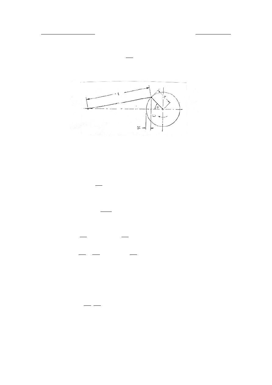
Now, consider the following figure:
θ
cos
r
r
x
−
=
where r is the radius of the crank.
or
t
r
r
x
ω
cos
−
=
∴ velocity of piston
θ
ω
sin
.
.r
dt
dx =
Acceleration of piston
θ
ω
cos
.
.
2
2
2
r
dt
x
d
=
Now,
s
s
p
s
a
A
r
a
A
f
f
.
cos
.
.
.
2
θ
ω
=
=
and
s
s
s
s
as
a
A
r
g
L
g
f
L
H
.
cos
.
.
.
.
2
θ
ω
=
=
This is maximum when
o
or
0
1
cos
=
=
θ
θ
, i.e., when piston is at its
dead centre.
(
)
r
a
A
g
L
H
s
s
as
.
.
.
2
max
ω
=
∴
Dr. Hussein Majeed Salih
Fluid Machinery
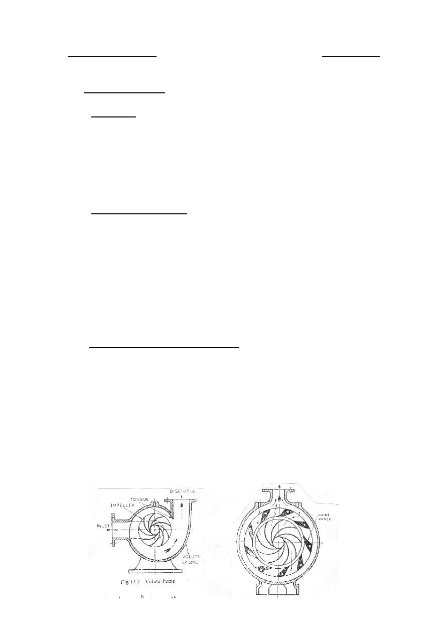
6.2
U
Centrifugal pumps
6.2.1
U
Definition
The hydraulic machines that convert mechanical energy into pressure
energy, by means of centrifugal force acting on the fluid are called as
"centrifugal pumps". The centrifugal pump is similar in construction to
Francis turbine. But the difference is that the fluid flow is in a direction
opposite to that in the turbine.
6.2.2
U
Principle of operation
The first step in the operation of a pump is priming that is, the suction
pipe and casing are filled with water so that no air pocket is left. Now the
revolution of the pump impeller inside a casing full of water produces a
forced vortex which is responsible for imparting a centrifugal head to the
water. Rotation of impeller effects a reduction of pressure of the centre.
This causes the water in the suction pipe to rush into the eye. The speed
of the pump should be high enough to produce centrifugal head sufficient
to initiate discharge against the delivery head.
6.2.3
U
Classificationof centrifugal pumps
Centrifugal pumps can be classified according to :
a) Working head
• Low lift centrifugal pumps (up to 15 m).
• Medium lift centrifugal pumps (15-40 m).
• High lift centrifugal pumps (above 40 m).
b) Type of casing
• Volute pump.
• Turbine pump or diffusion pump.
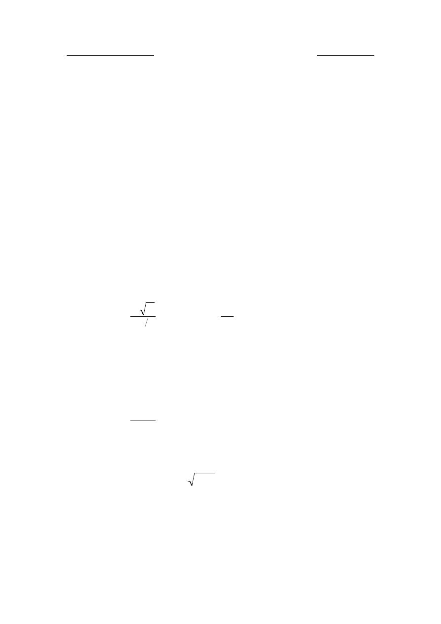
Dr. Hussein Majeed Salih
Fluid Machinery
c) Number of impeller
• Single stage centrifugal pump.
• Multi stage centrifugal pump.
d) Number of entrances to the impeller
• Single entry.
• Double entry.
e) Disposition of shaft
• Horizontal.
• Vertical.
f) Liquid handled.
g) Specific speed.
4
3
H
Q
N
N
s
=
,
g
v
H
2
2
=
h) Non-dimensional factor k
R
s
R
.
The specific speed N
R
s
R
is a dimensional quantity, but a k
R
s
R
is a non-
dimensional quantity.
3
2
.
v
N
Q
k
s
=
Q: flow rate.
(m
P
3
P
/s)
N: speed.
(rpm)
v: velocity of water
gH
2
=
( m/s) , H: total head.
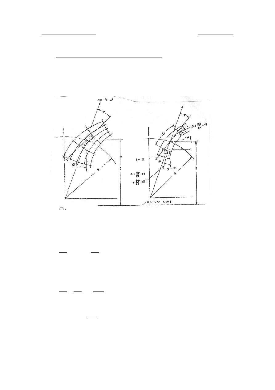
Dr. Hussein Majeed Salih
Fluid Machinery
6.2.4
U
Bernoulli's equation for relative motion
Consider the motion of fluid inside a turbine runner or an impeller of a
centrifugal pump.
For steady flow:
0
,
0
=
∂
∂
=
∂
∂
t
w
t
P
Acceleration in the direction of relative velocity w,
w
s
w
w
t
w
t
w
∂
∂
+
∂
∂
=
∂
∂
w
ds
dw
w
+
= 0
Mass of fluid accelerated
(
)
w
ds
l
b .
.
.
ρ
=

Dr. Hussein Majeed Salih
Fluid Machinery
Force acting on the element are:
• Weight
w
ds
l
b .
.
.
γ
=
.
• Centrifugal force
2
.
.
.
.
.
Ω
=
R
ds
l
b
w
ρ
.
• Pressure difference
(
) (
)
dl
l
b
dP
P
P
l
b
+
+
−
=
.
.
.
.
dP
l
b .
.
−
=
( neglecting dl)
Now resultant force in the direction of stream line:
= mass * acceleration
w
w
w
w
ds
dw
w
ds
l
b
R
ds
l
b
dP
l
b
ds
l
b
.
.
.
.
.
cos
.
.
.
.
.
.
.
.
cos
.
.
.
2
ρ
ψ
ρ
φ
γ
=
Ω
+
−
Simplifying
ψ
γ
φ
cos
.
.
.
cos
.
2
w
w
ds
g
R
dP
ds
g
dw
w
Ω
+
−
=
Sub.
dz
ds
w
−
=
φ
cos
.
and
dR
ds
w
=
ψ
cos
.
Then
dR
g
R
dP
dz
g
dw
w
.
.
.
2
Ω
+
−
−
=
γ
or
0
.
.
.
2
=
Ω
−
+
+
dR
g
R
dP
dz
g
dw
w
γ
integrating:
.
2
.
2
2
2
2
cons
g
R
P
z
g
w
=
Ω
−
+
+
γ
=
Ω
.
R
centrifugal velocity
(u)
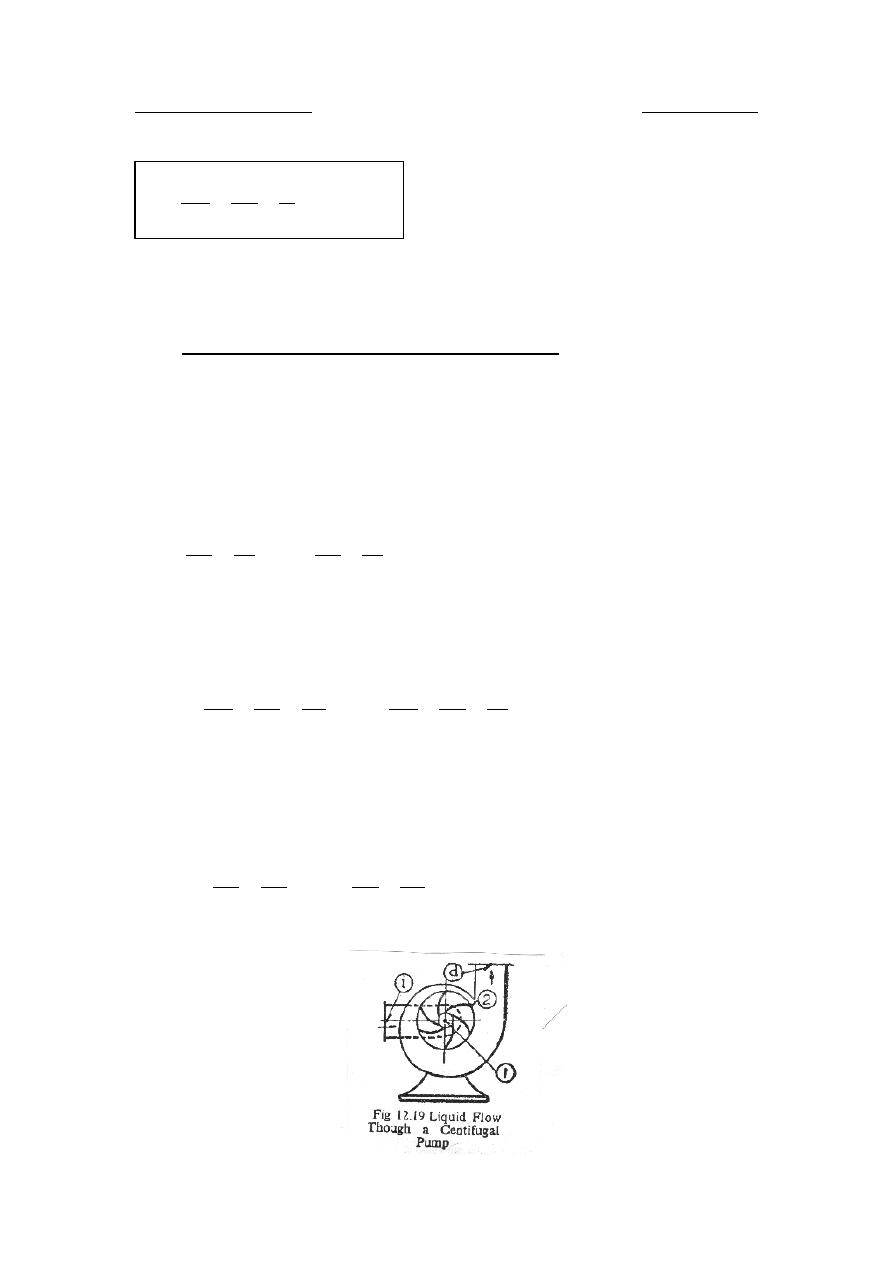
Dr. Hussein Majeed Salih
Fluid Machinery
( Bernoulli's equation for relative motion).
6.2.5
U
Fundamental equation of centrifugal pump
Consider the figure below. The equation of flow between any two
consecutive points can be obtained by applying the Bernoulli's theorem.
a) For flow from (i) to (1) i.e., through the stationary suction pipe,
since v
R
1
R
( absolute velocity of water).
)
1
(
2
1
1
2
1
2
2
−
−
+
+
=
+
+
i
L
i
i
i
H
z
P
g
v
z
P
g
v
γ
γ
b) From (1) to (2) i.e., through the movable impeller.
)
2
1
(
1
1
2
1
2
1
2
2
2
2
2
2
2
2
2
2
−
−
+
+
−
=
+
+
−
L
H
z
P
g
u
g
w
z
P
g
u
g
w
γ
γ
c) From (2) to (d) i.e., through the stationary casing inside which the
motion of water is absolute:
)
2
(
2
2
2
2
2
2
2
d
L
d
d
d
H
z
P
g
v
z
P
g
v
−
−
+
+
=
+
+
γ
γ
.
2
2
2
2
cons
z
P
g
u
g
w
=
+
+
−
∴
γ

Dr. Hussein Majeed Salih
Fluid Machinery
Now, adding the above three equations and re-arranging:
(
)
)
2
(
)
2
1
(
)
1
(
2
2
2
1
2
2
2
2
2
1
2
1
2
2
2
2
2
2
2
d
L
L
i
L
i
i
i
d
d
d
H
H
H
z
P
g
v
z
P
g
v
g
u
u
g
w
w
g
v
v
−
−
−
+
+
+
+
+
−
+
+
=
−
+
−
+
−
γ
γ
The first term on the right hand side is the gross manometric head of
the pump, while the second term stands for the total pump losses due
to the fluid resistance inside the pump only.
mano
mano
H
H
g
u
u
g
w
w
g
v
v
∆
+
=
−
+
−
+
−
∴
2
2
2
2
1
2
2
2
2
2
1
2
1
2
2
This is known as the fundamental equation of centrifugal pump.
Consider the manometric efficiency of the pump:
mano
mano
mano
mano
H
H
H
∆
+
=
η
mano
mano
H
g
u
u
g
w
w
g
v
v
η
=
−
+
−
+
−
∴
2
2
2
2
1
2
2
2
2
2
1
2
1
2
2
With aid of velocity triangles at inlet and outlet:
1
1
1
2
1
2
1
2
1
cos
2
α
v
u
v
u
w
−
+
=
2
2
2
2
2
2
2
2
2
cos
2
α
v
u
v
u
w
−
+
=
2
2
2
1
1
1
2
2
2
1
2
2
2
1
2
2
2
1
cos
2
cos
2
α
α
v
u
v
u
v
v
u
u
w
w
+
−
−
+
−
=
−
∴
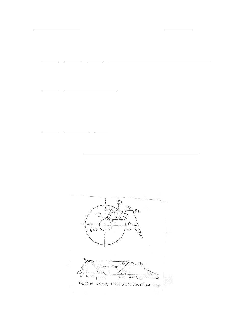
Dr. Hussein Majeed Salih
Fluid Machinery
Substituting this in fundamental equation:
g
v
u
v
u
v
v
u
u
g
u
u
g
v
v
H
mano
mano
2
cos
2
cos
2
2
2
2
2
2
1
1
1
2
2
2
1
2
2
2
1
2
1
2
2
2
1
2
2
α
α
η
+
−
−
+
−
+
−
+
−
=
g
v
u
v
u
H
mano
mano
1
1
1
2
2
2
cos
cos
α
α
η
−
=
Generally
0
cos
90
1
1
=
⇒
=
α
α
o
, neglecting prerotation.
g
v
u
g
v
u
H
u
mano
mano
2
2
2
2
2
cos
=
=
α
η
g
outlet
at
whirl
of
velocity
outlet
at
speed
Peripheral
H
mano
mano
*
*
η
=
∴
This is the form of the fundamental equation, which is used in
practice.

Dr. Hussein Majeed Salih
Fluid Machinery
6.2.6
U
Work done and manometric efficiency
Work done/sec by the pump impeller is:
(
)
2
2
1
1
.
.
u
u
v
u
v
u
Q
P
−
=
ρ
(kW)
The suffices (1) and (2) used in this equation will hold true if point (1)
denotes the pressure side and point (2) denotes suction side of the pump.
However if point (1) denotes inlet and point (2) the outlet of the pump
impeller, then the above equation will be written as:
(
)
1
1
2
2
.
.
u
u
v
u
v
u
Q
P
−
=
ρ
Since
o
90
1
=
α
( radial entrance)
0
cos
1
=
⇒
α
∴ The energy supplied to the fluid by the impeller per kN per sec is:
g
v
u
u2
2
=
and this is equal to the head generated, provided there is no losses inside
the pump.
i.e., Head generated by the pump=Difference between the total energy of
fluid at inlet and outlet of the pump
≅
M|anometric head.
mano
u
H
g
v
u
=
2
2
if there is no internal loss of the pump.
In practice there are always some head losses inside the pump.
mano
mano
u
H
H
g
v
u
∆
+
=
∴
2
2
mano
mano
mano
mano
H
H
H
∆
+
=
η

Dr. Hussein Majeed Salih
Fluid Machinery
but
g
v
H
H
H
d
f
static
mano
2
2
+
+
=
g
v
u
g
v
H
H
u
d
f
static
mano
2
2
2
2
+
+
=
∴
η
6.2.7
U
Pressure rise by pump impeller
Applying Bernoulli's theorem between inlet and outlet edge of impeller.
Energy at inlet = Energy at outlet – useful work done by impeller.
g
v
u
g
v
P
g
v
P
u2
2
2
2
2
2
1
1
2
2
−
+
=
+
γ
γ
∴ Pressure rise between outlet and inlet edges of impeller:
g
v
u
g
v
v
P
P
u2
2
2
2
2
1
1
2
2
+
−
=
−
γ
6.2.8
U
Efficiency of centrifugal pump
a) Overall efficiency
power
shaft
input
power
water
ouput
overall
=
η
This is known also "gross efficiency" or "actual efficiency"
P
R
shaft
R
= P
R
input to impeller
R
+ P
R
leakage
R
+ P
R
mech. loss
P
R
shaft
R
= B.P of driving unit – P
R
lost in coupling

Dr. Hussein Majeed Salih
Fluid Machinery
g
v
u
P
u
impeller
to
input
2
2
=
per kN per sec
= P
R
water
R
+ P
R
hydraulic
R
mano
water
H
Q
P
.
.
γ
=
(kW)
mano
hydraulic
H
Q
P
∆
=
.
.
γ
(kW)
= Power required to overcome head losses due to:
i. Circulatory or secondary flow.
ii. Frictions of volute and impeller.
iii. Turbulence.
P
R
leakage
R
= Power required to overcome leakage
R
.
P
R
mech. loss
R
= Power required to overcome mechanical losses
b) Mechanical efficiency
shaft
pump
the
to
input
power
water
the
to
impeller
the
by
delivered
power
mech
=
η
(
)
P
sh
P
P
sh
power
shaft
g
v
u
Q
Q
loss
mec
u
.
.
.
2
2
−
=
∆
+
=
γ
c) Volumetric efficiency
Q
Q
Q
Q
∆
+
=
η
where Q: discharge delivered by the pump
∆ Q : amount of leakage.

Dr. Hussein Majeed Salih
Fluid Machinery
d) Manometric efficiency
impeller
by
fluid
to
imparted
head
lift
gross
or
head
measured
actual
mano
=
η
g
v
u
H
g
v
u
g
v
H
H
u
mano
u
d
f
static
mano
2
2
2
2
2
2
=
+
+
=
∴
η
(
)
loss
mec
mano
P
P
sh
H
Q
Q
.
.
.
.
−
∆
+
=
γ
This is also known as hydraulic efficiency. From above:
mano
Q
mech
overall
η
η
η
η
.
.
.
=
6.2.9
U
Cavitation in pump
When the liquid is flowing in the pump, it is possible that the pressure at
any part of the pump may fall below the vapor pressure, then the liquid
will vaporize and the flow will no longer remain continuous. The
vaporization of the liquid will appear in the form of bubbles released in
the low pressure region of the pump. These bubbles are carried along
with water stream and when these pass through a region of high pressure,
these collapse suddenly. When the bubbles collapse on a metallic surface
such as tips of impeller blades, the cavities are formed. Successive bubble
collapsing at the same metallic surface produces pitting since penetration
in the grain boundaries take place. Once the pitting takes place, the liquid
rushes to fill the pits causing mechanical destruction and the liquid hits
the blades with such a great force that it damages the impeller. This
phenomena is known as "Cavitation". A great noise is experienced due to
cavitation leading to vibration of the pumping set.

Dr. Hussein Majeed Salih
Fluid Machinery
Since the cavitation occurs when the pressure falls below atmospheric,
the trouble is experienced mainly at the impeller vane inlet due to high
suction lift which must be brought within limits.
6.2.10
U
Net Positive Suction Head (NPSH)
(NPSH) is the head required at the pump inlet to keep the liquid from
cavitation or boiling. The pump inlet or suction side is the low pressure
point where cavitation will first occur.
γ
γ
vap
i
i
P
g
v
P
NPSH
−
+
=
2
2
Where P
R
vap
R
is the vapor pressure of the liquid. NPSH is also defined as a
measure of the energy available on the suction side of the pump. NPSH is
a commercial term used by the pump manufactures and indicates the
suction head which the pump impeller can produce. In other words, it is
the height of the pump axis from the water reservoir which can be
permitted for installation.
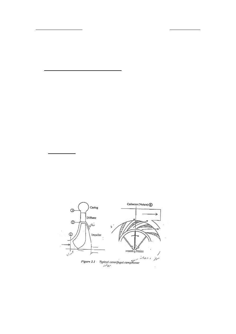
Dr. Hussein Majeed Salih
Fluid Machinery
Chapter Seven
Compressors
7.1
U
Centrifugal compressors and fans
Compressors as well as pumps and fans are the devices used to increased
the pressure of a fluid, but they differ in the tasks they perform. A fan
increase the pressure of a gas slightly and it is mainly used to move a gas
around. A compressor is capable of compressing the gas to very high
pressure. Pumps work very much like compressors except that they
handle liquids inside of gases.
Centrifugal compressors and fans are turbo-machines employing
centrifugal effects to increase the pressure of the fluid. The centrifugal
compressor is mainly found in turbo chargers.
7.1.1
U
components
• Impeller.
• Diffuser.
• Spiral casing (scroll or volute).
As shown in figure.
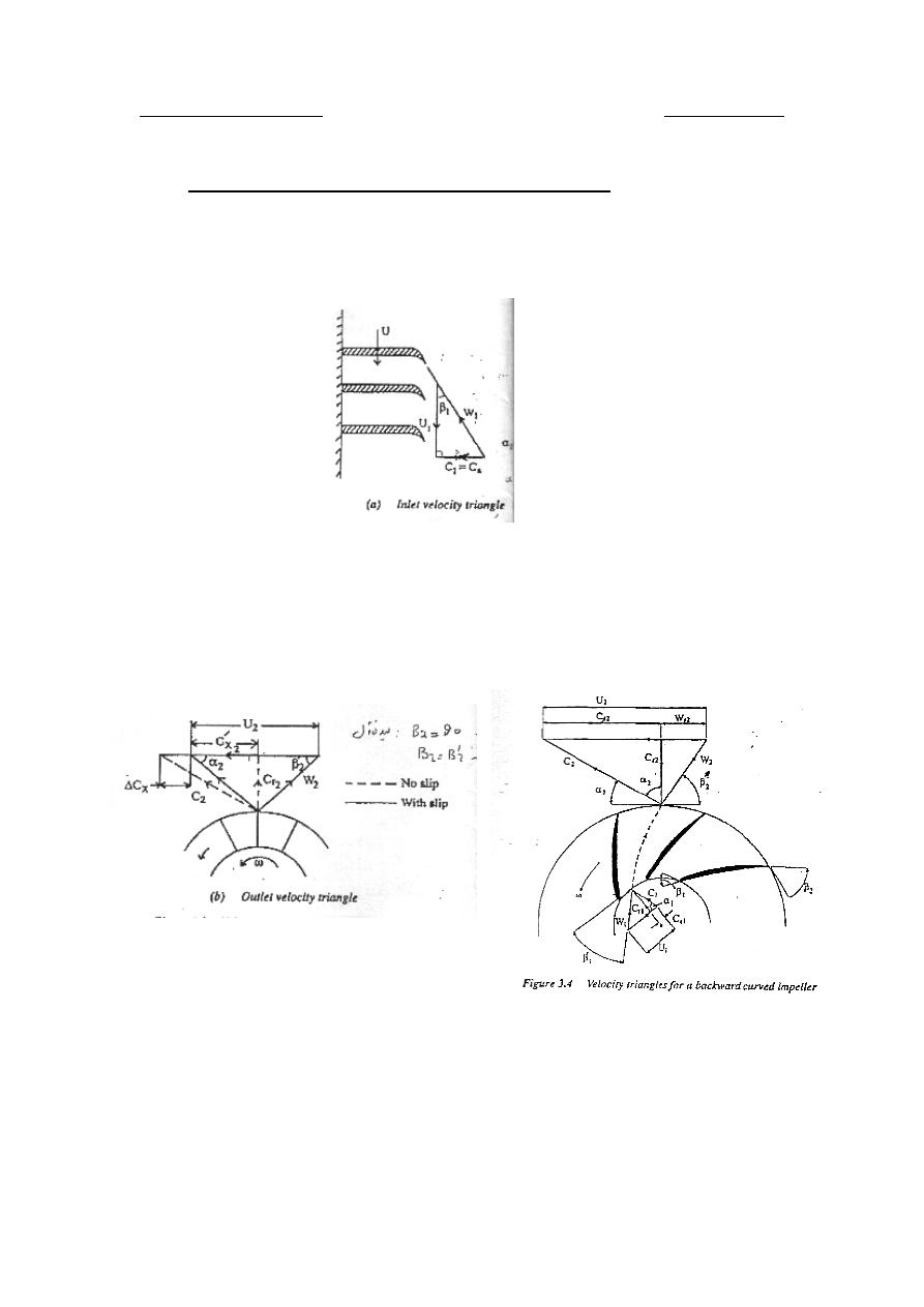
Dr. Hussein Majeed Salih
Fluid Machinery
7.1.2
U
Velocity diagrams for a centrifugal compressor
The gas enters the compressor at the eye, in an axial direction (
o
90
1
=
α
), as shown in figure below.
And for radial blade (
o
90
2
=
β
) as a result of slip, the relative velocity
vector (
2
W
) is at angle (
2
2
β
β
〈
′
), for zero slip (
o
90
2
=
β
)and so
(
)
2
2
U
C
x
=
and
(
)
2
2
W
C
r
=
, as shown in figure.
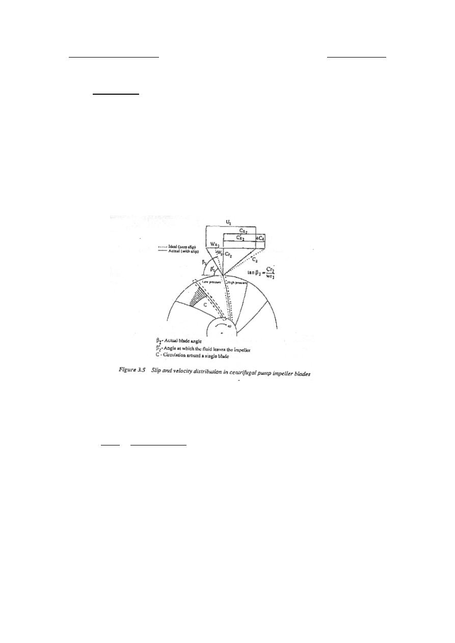
Dr. Hussein Majeed Salih
Fluid Machinery
7.1.3
U
Slip factor
The fluid leaves the impeller at an angle
2
β
′
other than the actual blade
angle
2
β
. This is due to "fluid slip". Angle
2
β
′
is less than angle
2
β
. In
centrifugal compressors, the air trapped between the impeller vanes is
reluctant to move around with the impeller, and this results in a higher
static pressure on the leading face of the vane than on the trailing face of
the vane. This problem is due to the inertia of the air. Then the air tends
to flow around the edges of the vanes in the clearance space between
impeller and casing.
Slip factor is defined as:
(
)
2
2
2
2
x
x
x
x
x
s
C
C
C
C
C
∆
−
=
′
=
σ
Referring to the above figure , for the no slip condition:
2
2
2
x
x
W
U
C
−
=
and
2
2
2
cot
.
β
r
x
C
W
=
,
2
2
2
2
cot
.
β
r
x
C
U
C
−
=
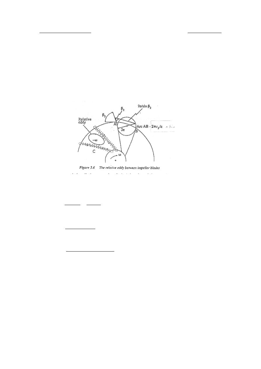
Dr. Hussein Majeed Salih
Fluid Machinery
Stodola proposed the existence of a relative eddy within the blade
passages as shown in figure below. By definition, a frictionless fluid
which passes through the blade passages have no rotation. Therefore at
the outer of the passage the rotation should be zero. Now, the impeller
has an angular velocity "
ω
" , so that, relative to the impeller, the fluid
must have an angular velocity "-
ω
" to match the zero-rotation condition.
e
C
x
.
ω
=
∆
∴
Assume
z
r
e
2
2
.
2
sin
2
π
β
=
z
U
C
x
2
2
2
sin
.
.
β
π
=
∆
∴
(
)
2
2
2
2
2
cot
.
sin
.
.
1
β
β
π
σ
r
s
C
U
z
U
−
−
=
∴
The Stodola slip factor equation gives best results for the blade angle in
the range
o
o
30
20
2
〈
〈
β
, for another angle range there are another
equations.

Dr. Hussein Majeed Salih
Fluid Machinery
7.1.4
U
Energy transfer
By Euler's pump equation, without slip
g
C
U
C
U
E
x
x
1
1
2
2
.
.
−
=
From inlet velocity triangle
0
1
=
x
C
, for ideal condition
2
2
x
C
U
=
, from
the outlet velocity triangle:
g
U
g
C
U
E
x
2
2
2
2
.
=
=
And with slip, the theoretical work is
g
U
E
s
2
2
.
σ
=
7.1.5
U
Power input factor
Power input factor or work factor, or stage loading coefficient:
plied
sup
work
l
Theoretica
plied
sup
work
Actual
=
ψ
ψ
typically takes values from 1.035-1.041
So, the actual energy transfer becomes:
g
U
.
.
E
s
2
2
σ
ψ
=
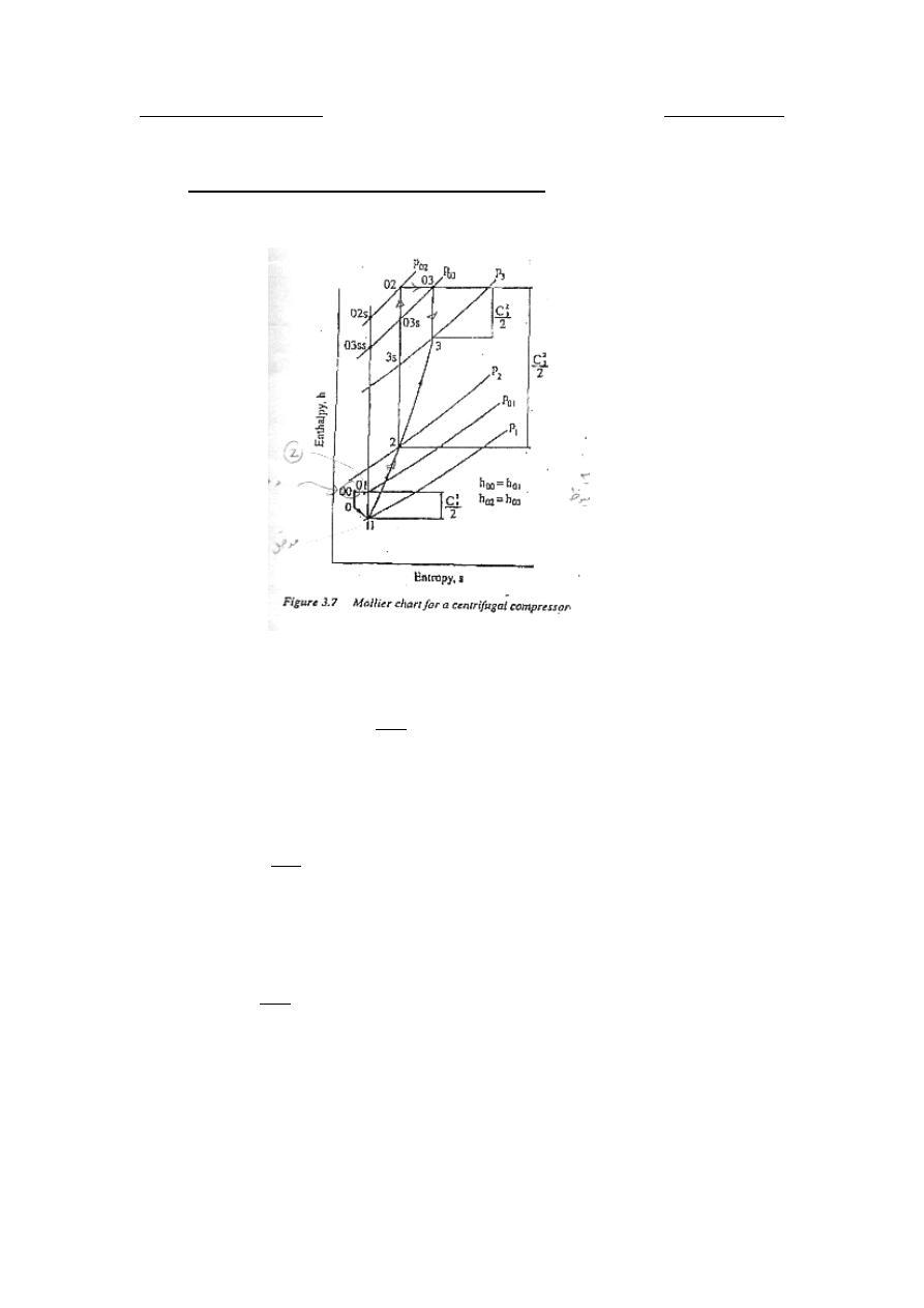
Dr. Hussein Majeed Salih
Fluid Machinery
7.1.6
U
The energy equation along a streamline
1. inlet casing
total enthalpy,
t
tan
cons
C
h
h
o
=
+
=
2
2
therefore, for the fluid drawn from the atmosphere into the inducer
section, the total enthalpy is:
2
2
o
o
oo
C
h
h
+
=
Total enthalpy at section -1, i.e., inlet of the impeller, is
2
2
1
1
1
C
h
h
o
+
=
And since no shaft work has been done and assuming that adiabatic
steady flow occurs

Dr. Hussein Majeed Salih
Fluid Machinery
1
o
oo
h
h
=
, thus
2
2
o
o
C
h
+
=
2
2
1
1
C
h
+
2. Impeller
Work is done on the fluid across the impeller and the static pressure is
increased from P
R
1
R
to P
R
2
R
. Writing the work done per unit mass on the
fluid in terms of enthalpy, we get:
1
2
o
o
h
h
m
/
W
−
=
From Euler's pump equation
1
1
2
2
x
x
C
.
U
C
.
U
m
/
W
−
=
Equating the two equation and after substituting for h
R
o
2
2
2
2
2
1
1
2
1
1
2
2
x
x
C
.
U
C
h
C
.
U
C
h
I
−
+
=
−
+
=
Where I is the impeller constant.
In general :
x
C
.
U
C
h
I
−
+
=
2
2
After substituting
2
2
2
x
r
C
C
C
+
=
and
2
2
2
x
r
W
W
C
−
=
and
rearrange:
2
2
2
2
U
W
h
I
−
+
=
Thus :

Dr. Hussein Majeed Salih
Fluid Machinery
2
2
2
2
2
1
2
1
2
2
1
2
W
W
U
U
h
h
−
+
−
=
−
Usually C
R
x2
R
=0 is assumed in preliminary design calculation.
2
2
1
2
U
.
.
h
h
s
o
o
σ
ψ
=
−
∴
Substituting
o
p
o
T
.
C
h
=
and rearranging the equation , we get:
p
s
o
o
C
U
.
.
T
T
2
2
1
2
σ
ψ
=
−
Where
p
C
is the mean specific heat over temperature range.
Since , no work is done in the diffuser,
3
2
o
o
h
h
=
and so
p
s
o
o
C
U
.
.
T
T
2
2
1
3
σ
ψ
=
−
Now define the isentropic efficiency.
its
lim
pressure
total
same
between
rise
enthalpy
Actual
outlet
and
inlet
between
rise
enthalpy
isentropic
Total
c
=
η
01
03
01
03
h
h
h
h
ss
−
−
=
Where the subscript "ss" represents the end state on the total pressure line
P
R
03
R
when the process is isentropic:

Dr. Hussein Majeed Salih
Fluid Machinery
01
03
01
03
T
T
T
T
ss
c
−
−
=
η
(
)
(
)
01
03
01
01
03
01
T
T
T
T
/
T
T
ss
−
−
=
But
(
)
1
01
03
01
03
−
=
γ
γ /
T
T
P
P
ss
(
)
(
)
1
01
01
03
1
−
−
+
=
γ
γ
η
/
c
T
T
T
(
)
1
01
2
2
1
−
+
=
γ
γ
σ
ψ
η
/
p
s
c
T
.
C
U
.
.
.
7.1.7
U
Stage pressure rise and loading coefficient
The static pressure rise in a centrifugal compressor occurs in the impeller,
diffuser and the volute. No change in stagnation enthalpy occurs in the
diffuser and volute.
01
02
h
h
plied
sup
Work
s
−
=
(
)
01
02
T
T
C
s
p
−
=

Dr. Hussein Majeed Salih
Fluid Machinery
−
=
1
01
02
01
T
T
T
.
C
s
p
(
)
−
=
−
1
1
01
02
01
γ
γ
/
p
P
P
T
.
C
(
)
(
)
1
1
0
01
−
=
−
γ
γ
/
p
R
T
.
C
Where R
R
o
R
is stagnation pressure ratio
From Euler's equation
2
2
x
C
.
U
plied
sup
Work
=
(
)
2
2
2
2
β
cot
C
U
U
r
−
=
−
=
2
2
2
2
2
1
β
cot
U
C
U
r
(
)
2
2
2
2
1
β
φ
cot
.
U
−
=
Where
2
φ
is the flow coefficient at the impeller exit
2
2
U
C
r
=
Equating the two equations:
(
)
(
)
1
1
0
01
−
−
γ
γ
/
p
R
T
.
C
(
)
2
2
2
2
1
β
φ
cot
.
U
−
=
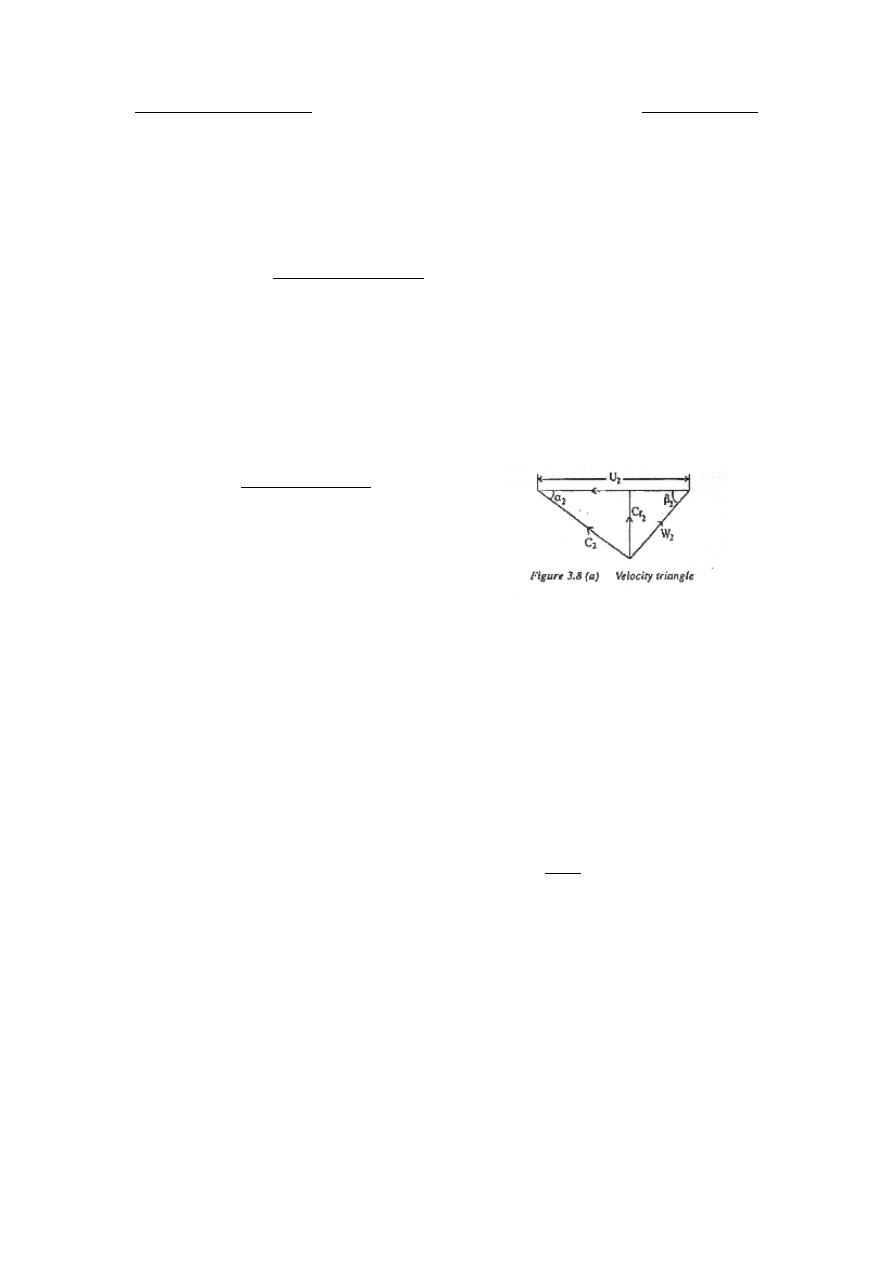
Dr. Hussein Majeed Salih
Fluid Machinery
Thus
(
)
(
)
1
01
2
2
2
2
0
1
1
−
−
+
=
γ
γ
β
φ
/
p
T
C
U
cot
.
R
The loading or pressure coefficient is defined as:
2
2
U
kg
/
done
Work
p
=
ψ
From the outlet velocity triangle
2
2
2
2
cot
.
β
r
x
C
U
C
−
=
From Euler's equation
2
2
x
C
.
U
g
.
E
=
Substitute
2
2
2
2
β
cot
.
C
U
C
r
x
−
=
and
2
2
2
U
C
r
=
φ
, yields :
(
)
2
2
1
β
φ
ψ
cot
.
p
−
=
Substitute this in stagnation pressure ratio equation R
R
0
R
:

Dr. Hussein Majeed Salih
Fluid Machinery
(
)
1
01
2
2
01
02
0
1
−
+
=
=
γ
γ
ψ
/
p
p
T
C
U
.
P
P
R
7.1.8
U
Pressure coefficient
The pressure or loading coefficient is also defined as the ratio of
isentropic work to Euler's work:
work
s
'
Euler
work
Isentropic
p
=
ψ
(
)
2
2
1
2
x
o
o
p
p
C
.
U
T
T
C
s
−
=
ψ
For radial vane impeller
2
2
U
C
x
=
(
)
2
2
1
2
U
T
T
C
o
o
p
p
s
−
=
∴
ψ
Now, isentropic work = actual work * isentropic efficiency
(
)
1
2
o
o
p
c
T
T
C
.
work
Isentropic
−
=
η
Then,
(
)
2
2
1
2
U
T
T
C
.
o
o
p
c
p
−
=
η
ψ

Dr. Hussein Majeed Salih
Fluid Machinery
But
(
)
2
2
1
2
U
.
.
T
T
C
s
o
o
p
σ
ψ
=
−
s
c
p
.
.
σ
ψ
η
ψ
=
∴
7.1.9
U
Degree of reaction
The degree of reaction of a centrifugal compressor stage is given by:
stage
the
in
enthalpy
stgnation
in
Change
impeller
the
in
enthalpy
static
in
Change
R
=
1
2
1
2
o
o
h
h
h
h
−
−
=
[
]
3
2
1
2
1
3
o
o
o
o
o
o
h
h
as
h
h
h
h
=
−
=
−
If the velocity of the gas approaching the compressor inlet is negligible
(
)
1
1
1
0
o
h
h
then
,
C
≅
≅
, and
2
2
2
2
2
C
h
h
o
−
=
(
)
(
)
1
2
2
2
1
2
2
o
o
o
o
h
h
/
C
h
h
R
−
−
−
=
∴
(
)
(
)
2
2
2
2
2
1
2
x
x
o
o
W
U
U
C
.
U
h
h
−
=
=
−
(
)
2
2
2
2
1
β
φ
cot
U
−
=
By substituting for
2
2
2
2
2
2
r
x
C
C
C
+
=
,
2
2
2
2
β
cot
C
U
C
r
x
−
=
, yields :

Dr. Hussein Majeed Salih
Fluid Machinery
(
)
(
)
[
]
(
)
2
2
2
2
2
2
2
2
2
2
2
2
2
2
2
1
1
2
1
1
β
φ
β
φ
φ
β
φ
cot
U
cot
U
cot
U
R
−
−
+
−
−
=
By some rearranging :
(
)
2
2
2
2
2
1
2
1
β
φ
β
φ
cot
ec
cos
R
−
−
=
For radial vane
o
90
2
=
β
, then
( )
1
1
2
1
2
2
=
−
=
p
and
,
R
ψ
φ
7.1.10
U
Effect of impeller blade shape on performance
The different blade shapes utilized in impellers of a centrifugal
compressors can be classified as :
a. Backward – curved blades.
o
90
2
〈
β
From outlet velocity triangle,
2
2
2
2
β
cot
C
U
C
r
x
−
=
And the energy transfer
g
C
.
U
E
x2
2
=
Thus
(
)
g
cot
C
U
.
U
E
r
2
2
2
2
β
−
=
or
gA
cot
mU
g
U
E
ρ
β
2
2
2
2
−
=
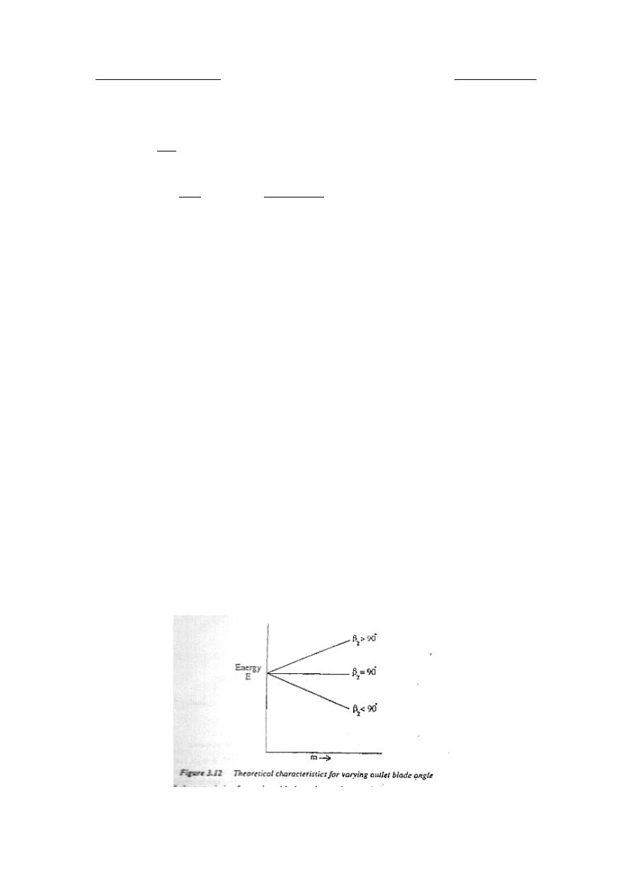
Dr. Hussein Majeed Salih
Fluid Machinery
where
2
r
C
A
m =
ρ
, the above equation is in the form of
bm
a
E
−
=
,
where
g
U
a
2
2
=
and
gA
cot
U
b
ρ
β
2
2
=
. As m increases , E decreases. The
characteristic is therefore falling.
b. Radial blades.
0
90
2
2
=
⇒
=
β
β
cot
o
a
E
=
∴
The energy transferred is constant at all flow rate and hence
characteristic is neutral.
c. Forward – curved blades.
o
90
2
〉
β
bm
a
E
+
=
∴
When m increases , E is increased. The characteristic will then be
raising .
The typical value of
2
β
for a multi-blades centrifugal fan is 140
P
o
P
.
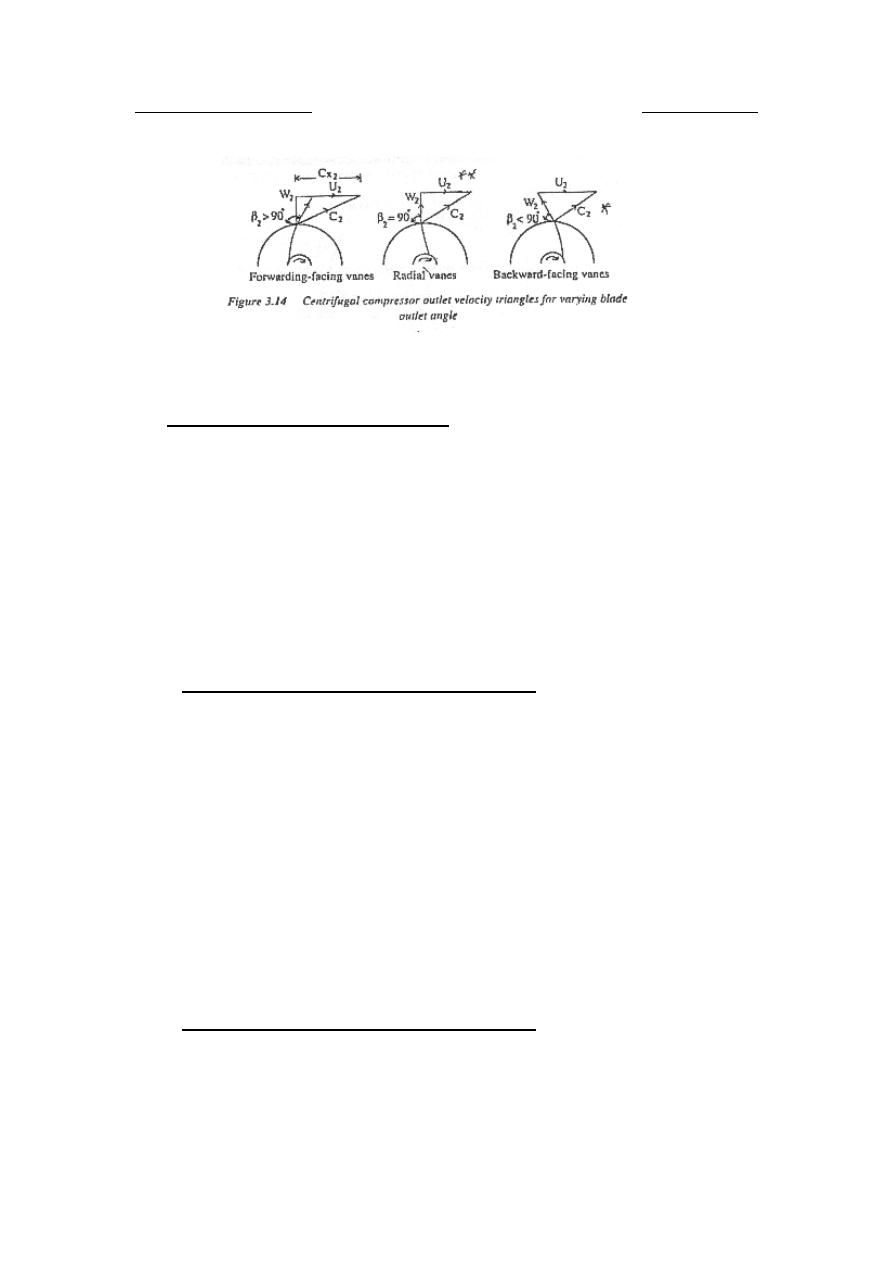
Dr. Hussein Majeed Salih
Fluid Machinery
7.2
U
Axial flow compressors and fans
Axial flow compressors and fans are turbo-machines that increase the
pressure of the gas flowing continuously in the axial direction. The
efficiency of the axial flow compressor is very sensitive to the mass flow
rate. Thus the axial flow compressor is ideal for constant load
applications such as in aircraft gas turbine engines. They are also used in
fossil fuel power stations, where gas turbines are used to meet the load
exceeding the normal peak load.
7.2.1
U
Advantages of an axial flow compressors
a. Axial flow compressor has higher efficiency than radial flow
compressor.
b. Axial flow compressor gives higher pressure ratio on a single shaft
with relatively high efficiencies.
c. Pressure ratio of 8:1 or even higher can be achieved using multi-
stage axial flow compressors.
d. The greatest advantage of the axial flow compressor is its high
thrust per unit frontal area.
e. It can handle large amount of air, inspite of small frontal area.
The main disadvantages are its complexity and coast.
7.2.2
U
Description of an axial flow compressors
An axial flow compressor consist of fixed and movable set of blades in
alternating sequence. Moving blades are attached to the periphery of a
rotor hub followed by fixed blades attached to the walls of the outer
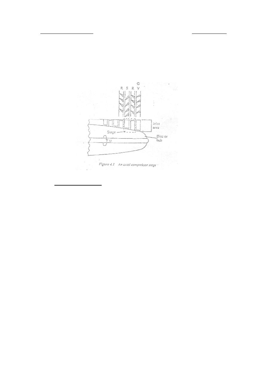
Dr. Hussein Majeed Salih
Fluid Machinery
casing as shown in the following figure. At the inlet of the compressor, an
extra row of fixed vanes called inlet guide vanes are fitted. These do not
form part of the compressor stage but are solely to guide the air at the
correct angle on to the first row of moving blades.
7.2.3
U
Working principle
The kinetic energy is imparted to the air by the rotating blades. Which is
then converted into a pressure rise. So, the basic principle of working is
similar to that of the centrifugal compressor. Referring to the previous
figure, the air enters axially from the right into the inlet guide vanes,
where it is deflected by a certain angle to impinge on the first row of
rotating blades with the proper angle of attack. The rotating vanes add
kinetic energy to the air. There is a slight pressure rise to the air. The air
is then discharged at the proper angle to the first row of stator blades,
where the pressure is further increased by diffusion. The air is then
directed into the second row of moving blades and the same process is
repeated through the remaining compressor stages. This process is shown
clearly by the following figure for the velocity triangles for an axial flow
compressor stage.
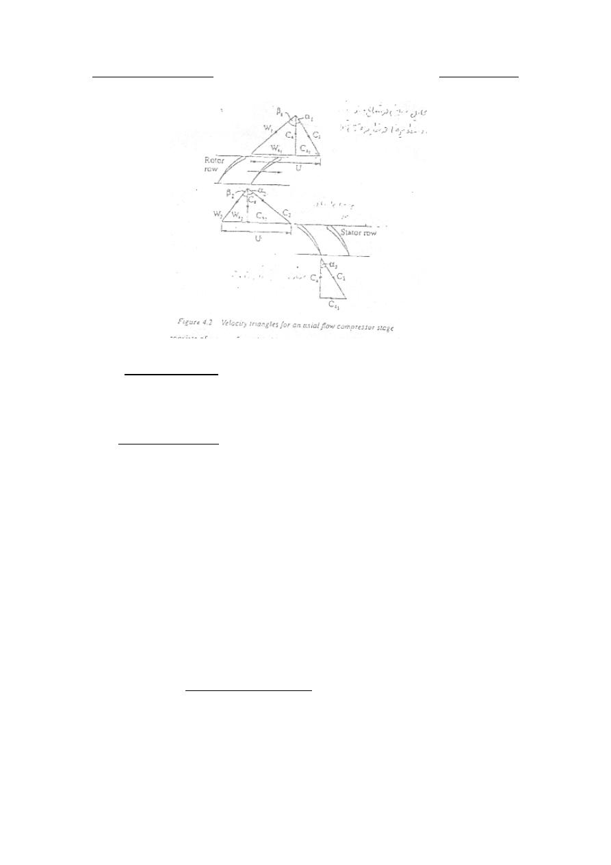
Dr. Hussein Majeed Salih
Fluid Machinery
7.2.4
U
Energy transfer
By Euler's equation:
g
C
.
U
C
.
U
E
x
x
1
1
2
2
−
=
From the velocity triangles, C
R
a
R
is constant through the stage and
U
R
1
R
=U
R
2
R
=U.
2
2
β
tan
C
U
C
a
x
−
=
and
1
1
β
tan
C
U
C
a
x
−
=
(
)
2
1
1
2
β
β
tan
tan
C
C
C
a
x
x
−
=
−
Therefore
(
)
g
tan
tan
C
.
U
E
a
2
1
β
β
−
=
The energy transfer may also be written in terms of the absolute velocity
flow angles.
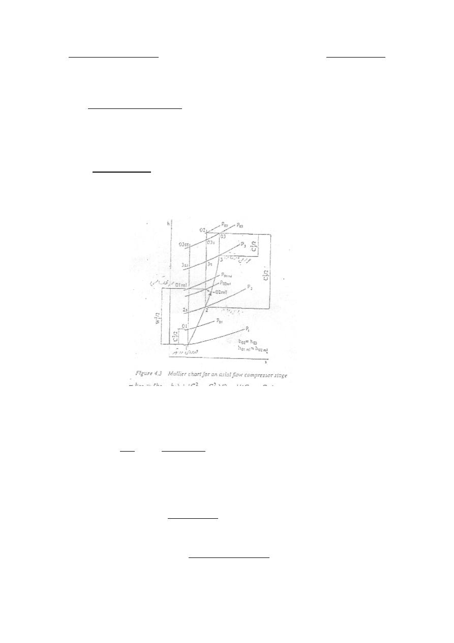
Dr. Hussein Majeed Salih
Fluid Machinery
(
)
g
tan
tan
C
.
U
E
a
1
2
α
α
−
=
7.2.5
U
Mollier chart
The flow through the axial flow compressor stage is shown
thermodynamically on the Mollier chart as shown in the following figure.
1
2
o
o
h
h
g
.
E
−
=
(
)
2
2
2
2
2
x
a
o
C
C
h
C
h
h
+
+
=
+
=
Then,
(
)
(
)
(
)
1
2
2
1
2
2
1
2
1
2
2
x
x
x
x
o
o
C
C
U
C
C
h
h
h
h
−
=
−
+
−
=
−
or
(
) (
)
(
)
[
]
0
2
2
1
2
1
2
1
2
=
−
−
−
−
−
x
x
x
x
C
C
U
C
C
h
h

Dr. Hussein Majeed Salih
Fluid Machinery
substituting for
2
2
x
x
W
C
U
=
−
,
1
1
x
x
W
C
U
=
−
and rearrange :
(
)
(
)
0
2
2
1
2
2
1
2
=
−
+
−
x
x
W
W
h
h
Since C
R
a
R
is constant , then
(
) (
)
2
1
2
2
2
1
2
2
W
W
W
W
x
x
−
=
−
, therefore:
2
2
2
1
1
2
2
2
W
h
W
h
+
=
+
Rewrite the change in enthalpy for a centrifugal compressor :
2
2
2
2
2
1
2
1
2
2
1
2
W
W
U
U
h
h
−
+
−
=
−
The comparison between the above two equations, indicates why the
enthalpy change in a single stage axial flow compressor is so low
compared to the centrifugal compressor. The relative velocities may be of
the same order of magnitude, but the axial flow compressor receives no
contribution from the change in tangential velocity (U).
Now, the isentropic or overall total-to-total efficiency is written as:
input
work
Actual
input
work
isentropic
Ideal
c
=
η
its
lim
pressure
total
same
the
between
rise
enthalpy
Actual
stage
the
in
rise
enthalpy
isentropic
Toatal
=
1
3
1
3
o
o
o
ss
o
h
h
h
h
−
−
=

Dr. Hussein Majeed Salih
Fluid Machinery
Which reduces to:
(
)
(
)
1
3
1
3
1
1
o
o
o
ss
o
o
c
T
T
T
/
T
T
−
−
=
η
Putting
1
1
3
1
3
−
=
γ
γ
o
ss
o
o
o
T
T
P
P
The pressure ratio becomes:
1
1
1
3
1
3
1
−
−
+
=
γ
γ
η
o
o
o
c
o
o
T
T
T
P
P
Where
(
)
p
a
o
o
C
tan
tan
C
.
U
T
T
2
1
1
3
β
β
−
=
−
The energy input to the fluid will be absorbed in raising the pressure and
velocity of the air and some will be wasted in overcoming various
frictional losses.
7.2.6
U
Work done factor
In practice "C
R
a
R
" is not constant along the length of the blade , thus the
work done factor is introduced. It is defined as:
capacity
absorbing
work
Ideal
capacity
absorbing
work
Actual
=
λ

Dr. Hussein Majeed Salih
Fluid Machinery
Hence,
(
)
p
a
o
o
C
tan
tan
C
.
U
.
T
T
2
1
1
3
β
β
λ
−
=
−
7.2.7
U
Stage loading or pressure coefficient
2
mU
input
Work
p
=
ψ
(
)
U
C
C
U
h
h
x
x
o
o
p
1
2
2
1
3
−
=
−
=
λ
ψ
(
)
1
2
α
α
λ
tan
tan
U
C
a
−
=
(
)
1
2
α
α
φ
λ
ψ
tan
tan
.
.
p
−
=
, where
φ
is the flow coefficient.
7.2.8
U
Reaction ratio
stage
in
rise
enthalpy
Static
rotor
in
rise
enthalpy
Static
R
=
1
3
1
2
h
h
h
h
−
−
=

Dr. Hussein Majeed Salih
Fluid Machinery
Since,
2
2
2
2
1
1
2
W
W
h
h
−
=
−
Also if C
R
1
R
=C
R
3
R
then,
(
)
1
2
1
3
1
3
x
x
o
o
C
C
U
h
h
h
h
−
=
−
=
−
and substituting for (h
R
2
R
-h
R
1
R
) and (h
R
3
R
-h
R
1
R
), yields :
(
)
1
2
2
2
2
1
2
x
x
C
C
U
W
W
R
−
−
=
(
) (
)
(
)
1
2
2
2
2
2
1
2
2
x
x
x
a
x
a
C
C
U
W
C
W
C
−
+
−
+
=
(
)(
)
(
)
1
2
2
1
2
1
2
x
x
x
x
x
x
C
C
U
W
W
W
W
−
−
+
=
But
2
2
x
x
W
U
C
−
=
and
1
1
x
x
W
U
C
−
=
, therefore:
2
1
1
2
x
x
x
x
W
W
C
C
−
=
−
Hence,
(
)
U
W
W
R
x
x
2
2
1
+
=
(
)
m
a
a
tan
U
C
U
tan
tan
C
β
β
β
=
+
=
2
2
1
m
tan
R
β
φ
=
∴

Dr. Hussein Majeed Salih
Fluid Machinery
Where ,
(
)
2
2
1
β
β
β
tan
tan
tan
m
+
=
and
m
β
is the mean relative velocity vector angle.
By some arrangement, one can verify :
(
)
2
1
1
2
α
β
φ
tan
tan
R
−
+
=
and
(
)
2
1
2
1
α
β
φ
tan
tan
R
−
+
=
For the case of incompressible and reversible flow :
1
3
1
2
P
P
P
P
R
−
−
=
7.2.9
U
Effect of reaction ratio on the velocity triangles
U
Case – 1
U
when R=0.5
The reaction ratio R is
(
) (
)
1
2
2
3
1
2
h
h
h
h
h
h
R
−
+
−
−
=
When R=0.5
(
) (
)
2
3
1
3
h
h
h
h
−
=
−
For a reaction ratio of 50% , the static enthalpy and temperature increase
in the stator and rotor are equal.
(
)
2
1
1
2
α
β
φ
tan
tan
R
−
+
=
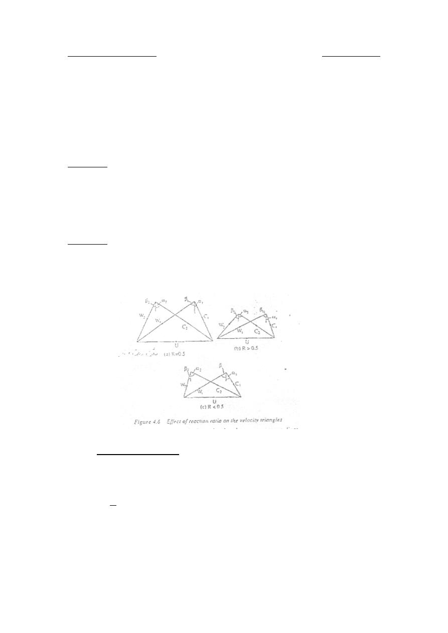
Dr. Hussein Majeed Salih
Fluid Machinery
When R=0.5 , thus
1
2
α
β
=
So, when the outlet and inlet velocity triangles are superimposed, the
resulting velocity diagram is symmetrical.
U
Case – 2
U
when
5
0.
R
〉
From the previous equation for R , it is seen that
1
2
α
β
〉
, therefore, the
static enthalpy rise in the rotor is greater than in the stator.
U
Case – 3
U
when
5
0.
R
〈
1
2
α
β
〈
, and the static enthalpy rise and pressure rise are greater in the
stator than in the rotor.
7.2.10
U
Static pressure rise
The main function of a compressor is to raise the static pressure of the air:
(
)
2
2
2
1
1
2
2
1
W
W
P
P
−
=
−
ρ

Dr. Hussein Majeed Salih
Fluid Machinery
Across the stator row:
(
)
2
3
2
2
2
3
2
1
C
C
P
P
−
=
−
ρ
Adding the above two equations, and considering a normal stage
(
)
1
3
C
C
=
, gives:
(
)
(
) (
)
2
1
2
1
2
2
2
2
1
3
2
C
W
W
C
P
P
−
+
−
=
−
ρ
( )
( )
( )
stator
rotor
stage
P
P
P
∆
+
∆
=
∆
∴
From the velocity triangles, the cosine rule gives:
−
−
+
=
β
π
2
2
2
2
2
cos
UW
W
U
C
And
x
W
sin
W
=
β
, then
x
UW
U
W
C
2
2
2
2
−
=
−
Substituting this equation in the stage pressure difference equation,
yields:
(
)
(
) (
)
1
2
2
2
1
3
2
2
2
x
x
UW
U
UW
U
P
P
−
−
−
=
−
ρ
(
)
2
1
2
x
x
W
W
U
−
=
From the velocity diagram , we get:
U
U
U
=
=
2
1

Dr. Hussein Majeed Salih
Fluid Machinery
2
2
1
1
x
x
x
x
C
W
C
W
+
=
+
∴
or
1
2
2
1
x
x
x
x
C
C
W
W
−
=
−
(
)
(
)
1
3
1
2
1
3
h
h
C
C
U
P
P
x
x
−
=
−
=
−
∴
ρ
Since, for an isentropic process :
ρ
dP
dh
Tds
−
=
= 0
and therefore
( )
ρ
P
h
s
∆
=
∆
The pressure rise in the real stage ( involving irreversible process) can be
determined if the isentropic ( stage) efficiency is known.