Industrial Engineering (IE)
Dr. Khallel Ibrahim Mahmoud
University of Technology
Electro-mechanical Engineering Dept.
Introduction
Production and
Productivity
Break Even Analysis(B.E)
Lec.N
o(1)
2011

Industrial Engineering (IE) - Dr. Khallel
Ibrahim Mahmoud
Introduction:
1.1 Concept of Industrial Engineering (IE)
Industrial Engineering is concerned with the design,
Improvement, and installation of integrated system of men,
material, and machines for the benefit of mankind .It draws
upon specialized knowledge and skills in the mathematical
and physical sciences together with the principles and
methods of engineering analysis and design to specify,
predict and evaluate the results to be obtained from such
systems.
1.2 IE Objectives
The basic objectives of Industrial Engineering are:
1- Improving operating methods and controlling costs.
2- Reducing these costs through cost reduction programs.
The aim of IE department is to provide specialized services
to production departments, such as methods improvement,
time study, Job evaluation and merit rating and to head new
projects if required.
1.3 IE Activities
Basic activities of industrial engineering as stated to
American Institute of industrial engineering as follows:
1- Processes (and methods) selection.
2- Selection and design of tools and equipment.
2

Industrial Engineering (IE) - Dr. Khallel
Ibrahim Mahmoud
3- Facilitates planning, plant location, materials handling and
storage facilities.
4- System design for planning and control of production
inventory, quality, and plant maintenance and distribution.
5- Cost analysis and control.
6- Develop time standards and performance standards.
7- Value engineering and analysis system design and install.
8- Mathematical tools and statistical analysis technia.
9- Performance evaluation.
10- Project feasibility studies.
1.4 IE Approach
Industrial engineering department uses scientific
approaching identifying and solving the problems .It collects
factual information regarding the problem analysis the
problem, prepares alternative solutions taken into account all
the internal and external constraints, selects the best
solution for implementation.
This stage is called problem identification .It consists of the
following steps:
1) Collect all details about the job, using standard recording
techniques like charts, diagrams, models and templates.
2) Recorded facts are subjected to critical examination using
a series of questions.
3) Find alternative solutions for the problem.
3

Industrial Engineering (IE) - Dr. Khallel
Ibrahim Mahmoud
4) Evaluate the alternatives and find the best solution.
Next the industrial engineering department makes
recommendation for the implementation of the best
alternatives so that the
1.5 Techniques of Industrial Engineering
The main aim of tools and techniques of industrial
engineering is to improve the productivity of the organization
by optimum utilization of organizations resources: men,
materials, and machines. The major tools and techniques
used in industrial engineering are:
1) Production planning and control.
2) Inventory control.
3) Job evaluation.
4) Facilitates planning and material handling.
5) System analysis.
6) Linear programming.
7) Simulation.
8) Network analysis (PERT, CPM).
9) Queuing models.
10) Assignment.
11) Sequencing and transportation models.
12) Games theory and dynamic programming.
13) Group technology.
4

Industrial Engineering (IE) - Dr. Khallel
Ibrahim Mahmoud
14) Statistical techniques.
15) Quality control.
16)
17) Decision making theory.
18) Replacement models.
19) Assembly line balancing.
20) MRP-JIT-ISO-TQM.etc.
1.6 The six standards phases of IE:-
1- Formulating the problem.
2- Constructing a mathematical model to represent the
system under study.
3- Deriving a solution from the model.
4- Testing the model and the solution derived from it.
5- Establishing controls over the solution.
6- Putting the solution to work: Implementation.
2- Productivity
The standard of living of industrialized nations depends upon
the economic efficiency of all its industrial enterprise great or
small.
2.1 Introduction/Definition of productivity
5
Industrial Engineering (IE) - Dr. Khallel
Ibrahim Mahmoud
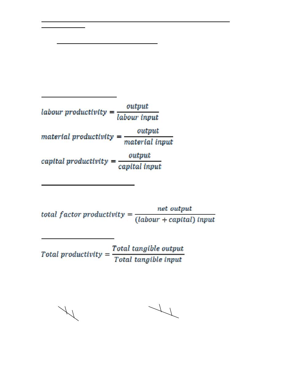
Productivity can be defined as the ratio of output in a period
of time to the input in the same period time. Productivity can
thus be measured as:
Productivity =
In simple terms productivity is the quantitative relationship
between what we produce (output) and the resources
(inputs) which we used.
2.2 Productivity and production:
Production is the process of converting the raw materials
into finished products by performing a set of manufacturing
operations in a predetermined sequence. Production refers
to absolute output. Thus, if the input increases the output will
normally increase in the same proportion. The productivity
remains unchanged if however the output increases with the
input of the resources, the productivity increases production
means the output in terms of money without any regard to
the input of resources , which productivity is a human
attitude to produce more and more with less input of
resources. There are six cases to increase the productivity
as shown
output +
+
c ++% -%
input - c - +% --%
2.3 Types of production systems:
6
Industrial Engineering (IE) - Dr. Khallel
Ibrahim Mahmoud
A production system consists of plant facilitates, equipment
and operating methods arranged in a systematic order. This
arrangement depends upon the type of product and the
strategy that a company employs to serve its customers.
There are two major types of production systems:
i) Make to stock production.
ii) Make to order production.
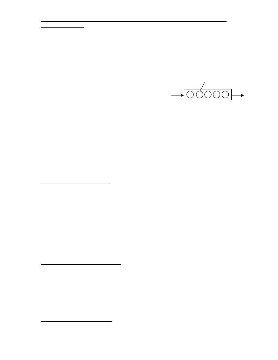
In make to stock production the products are manufactured
kept as ready stock and supplies to customers as orders are
operatio
input
output
system
Examples of such items are nuts, bolts, bearings, screws,
etc.
In make to order production the products are made only
Types of production
The production or manufacturing systems are classified as
follows:
a) Job type production.
b) Batch production.
c) Continuous or mass production.
a) Job type production.
It is characterized by high variety, low volume production,
producing one or a few products specially designed and
produced according to customer specifications like aircraft,
ships, special train.
b) Batch production.
7
Industrial Engineering (IE) - Dr. Khallel
Ibrahim Mahmoud
Here the product similar in design but different in size and
capacities are produced in batches of one size and capacity
at one time, at regular interval and stocked at warehouses a
waiting sales. Examples as pumps, motor etc, of different
capacities and types manufactured in batches.
c) Mass (Repetitive) production.
This production is characterized by high volume low variety
in this system several standard products are produced in
large quantity and stocked in warehouse awaiting dispatch
examples of such production, nuts bearings, t-shirts, etc.
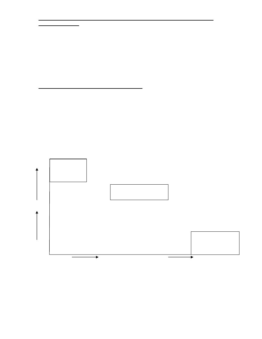
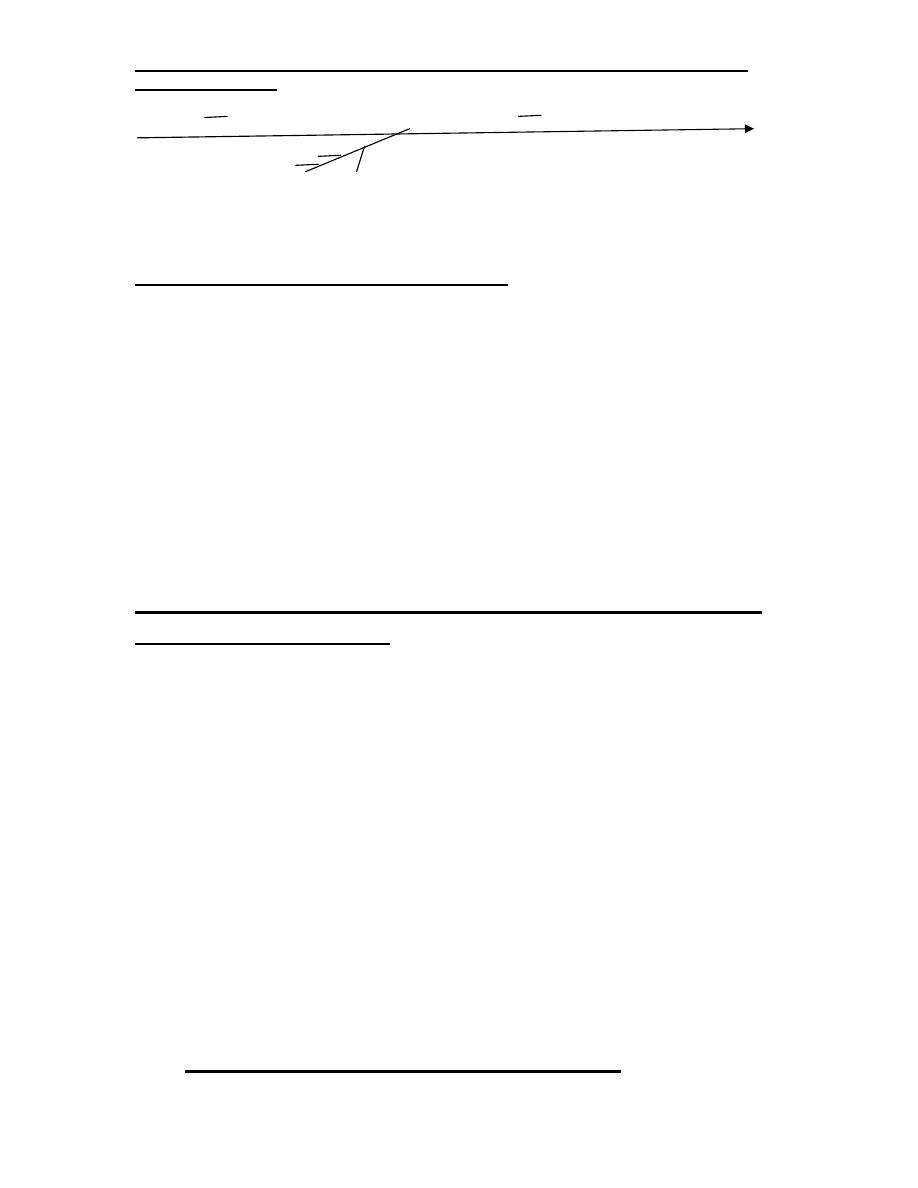
The following fig. shows volume variety relation for different
types of manufacturing systems.
Low Production volume
High
Job type
Batch production
Mass
Production
High
Variet
y
Low
After this brief introduction to types of production system and
productivity let us discuss how the productivity measured
and improved.
8
Industrial Engineering (IE) - Dr. Khallel
Ibrahim Mahmoud
2.4
Measurement of productivity
Productivity measures:
There are three major types of productivity measures as
listed below:
1- Partial productivity
2- Total factor productivity
It is the ratio of net output to the sum of associate …..
3- Total productivity:
Tangible means measurable for total tangible input =value of
human, material, capital, energy and other inputs used.
Man power material
9
Industrial Engineering (IE) - Dr. Khallel
Ibrahim Mahmoud
P
Machines
5- Factors affecting productivity:
1. Raw material, its nature and quality.
2. Utilization of manpower.
3. Utilization of plant, equipment and machinery.
4. Basic nature of manufacturing processes employed.
5. Efficiency of plant.
6. Volume, capacity, and uniformity of production.
6- The ways in which the productivity can be increased
summarized as under:
1) Increase manpower effectiveness at all levels.
2) Method improvement.
3) Improve basic production processes by research and
development.
4) Use better production equipment.
5) Improve / simplify product design and reduce variety.
6) Better production planning and control
.
2.1
Productivity Improvement Techniques
10

Industrial Engineering (IE) - Dr. Khallel
Ibrahim Mahmoud
1) Technology based
a. CAD/CAM/CIMS
b. Robotics.
c. Laser technology.
d. Modern maintenance technology.
e. Energy technology.
f. Flexible manufacturing system (FMS).
2) Employee based
a. Incentives
b. Promotion
c. Job design
d. Quality circle
3) Material based
a. Material planning and control
b. waste elimination
c. Recycling and reuse of waste materials
d. Purchasing Logistics
4) Process based
a. Method engineering and work simplification
b. Process design
11

Industrial Engineering (IE) - Dr. Khallel
Ibrahim Mahmoud
c. Human factors engineering
5) Product based
a. Reliability engineering
b. Product mix and promotion
c. Value analysis/value engineering.
6) Management based
a. Management technique
b. Communication
c. Work culture
d. Motivecation
e. Promoting group activity
Questions:
1. Write short notes on:
a) Techniques of Industrial engineering (Ans. 1.5)
b) Productivity measurement models (Ans. 2.4)
2. Define the term productivity. How is it different from
production? Give examples using your own numb (Ans.
2.1, 2.2)
3. There are six cases to increase the production. Explain in
brief. (Ans. 2.2)
12
Industrial Engineering (IE) - Dr. Khallel
Ibrahim Mahmoud
4. Summarize the ways in which the productivity can be
increased. (Ans. 2.6)
5. Discuss the factors that affect productivity. (Ans. 2.5)
6. Write short notes on productivity improvement techniques.
(Ans. 2.7)
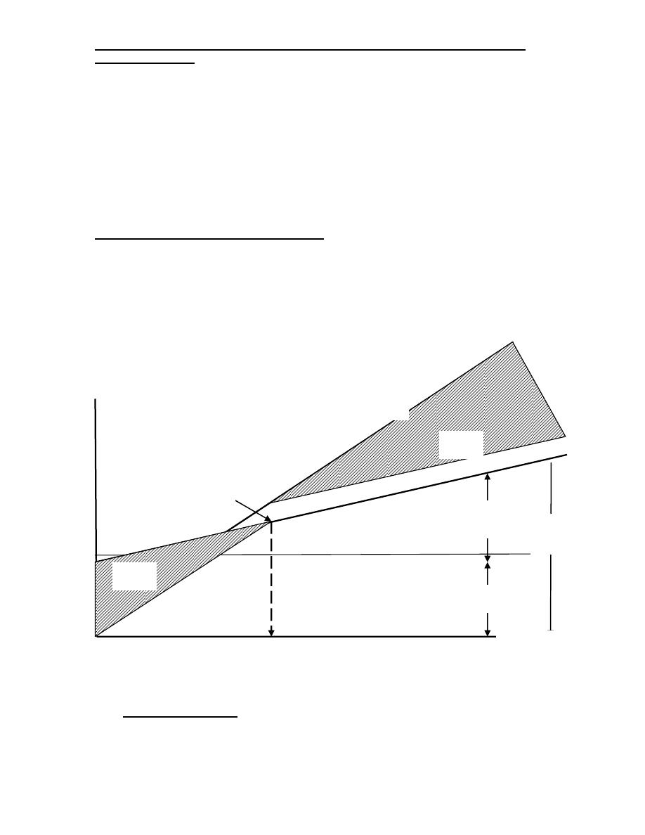
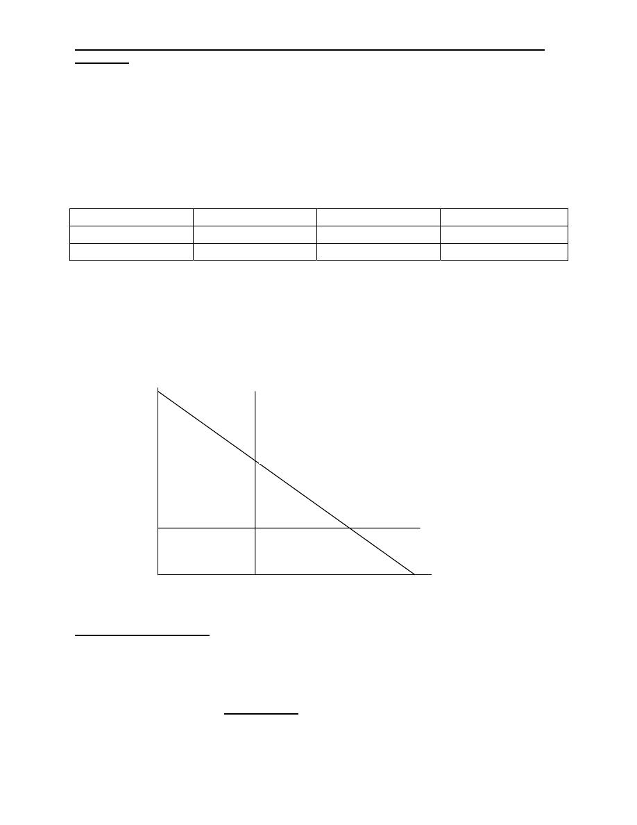
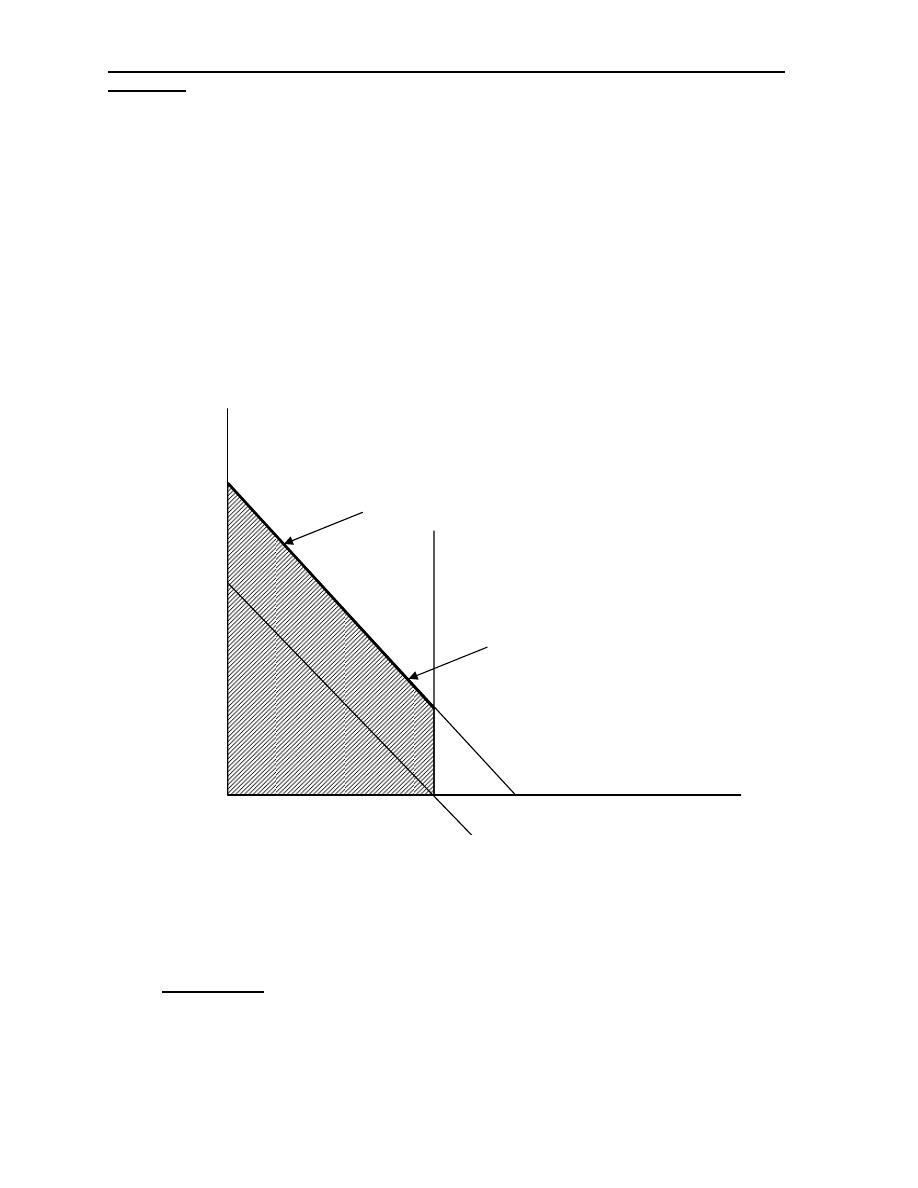
3- Break-Even analysis (B-E)
Break even production …….
At which the production cost equals income from sales. By
this value the company sets profit and below this value
suffers a loss.
Fig. Break-Even Point (B.E.P)
Cost
Production
volume
Revenue
curve
Profit
Loss
Total
cost
Total
v.cos
F.cos
t
Cost
curve
B.E.
P
Q
3.1 Steps in B.E.P
To construct break-even point, we must know:
13

Industrial Engineering (IE) - Dr. Khallel
Ibrahim Mahmoud
- Total fixed expenses at a certain target production.
- Total variable cost at the same target production.
- Total sales value at the same target production.
We find that the initially zero production rate, fixed cost will
remain as it is variable cost will be zero. The company still
suffers a loss equal to its fixed cost. As production volume
increases this loss decreases but the break-even point……
3.2 Assumptions
a) All the units remains fixed for any production volume.
b) Variable cost increase is linear.
c) Selling prices will remain constant at all levels.
d) Production and sales quantities are equal.
3.3 Formulation of linear Break-even model
This will define the minimum quantity that should be
produced without any loss or profit.
Notations:
Let Q: the quantity sold
b: price (the income per unit)
R: bQ (Revenue or income)
F: fixed cost
v: variable cost per unit
p: profit
Tc: total cost = F + vQ
14

Industrial Engineering (IE) - Dr. Khallel
Ibrahim Mahmoud
P= R-Tc
Quantity increase in price by making:
- Better
product.
- Advertisement.
- New product limited by market price.
Increase in planned quantity: Increase share of market
and increase those products with high profit or increase
share of market with the increase price according to
quantity of market.
Ref: - M.I.Khan , Industrial Engineering ,2
nd
Edition ,2008
- Maynard,H.B ,”Industrial Engineering
Handbook ,new York ,2004
15
Industrial Engineering (IE) - Dr. Khallel Ibrahim
Mahmoud
Industrial Engineering
(IE)
Dr. Khallel Ibrahim Mahmoud
University of Technology
Electro-mechanical Engineering Dept.
Lec.
N
o
(2)
Linear Programming
Model
2011
Industrial Engineering (IE) - Dr. Khallel Ibrahim
Mahmoud
Linear Programming
LP is a mathematical modeling technique designed to optimize the usage of limited
resources, such as available materials, labour and machine time.
The LP model includes three basic elements:
- Decision variables that we seek to determine.
- Objective (goal) that we aim to optimize.
- Constraints that we need to satisfy.
Steps in formulating LP problems:
1- Define the objective.
2- Define the decision variables.
3- Write the mathematical function for the objective (objective function).
4- Write a one- or two- word description of each constraint.
5- Write the right – hand side (RHS) of each constraint, including the unit of
measure.
6- Write ≤, = or ≥ for each constraint.
7- Write all the decision variables on the left-hand side of each constraint.
8- Write the cofficient for each decision variable in each constraint.
Formulation of linear programming model (LP)
The general form of each model will be:
Z= c
1
x
1
+ c
2
x
2
+……. c
k
x
k
Subject to:
a
11
x
1
+ a
12
x
2
+……. a
1k
x
k
b
1
a
21
x
1
+ a
22
x
2
+……. a
2k
x
k
b
2
a
m1
x
1
+ a
m2
x
2
+……. a
mk
x
k
b
1
Industrial Engineering (IE) - Dr. Khallel Ibrahim
Mahmoud
where: C
j
is a known (cost or profit) coefficient X
j
.
X
j
is an unknown variable.
a
ij
is a known constant.
b
j
is a known constant.
≤, = or ≥ for each constraint.
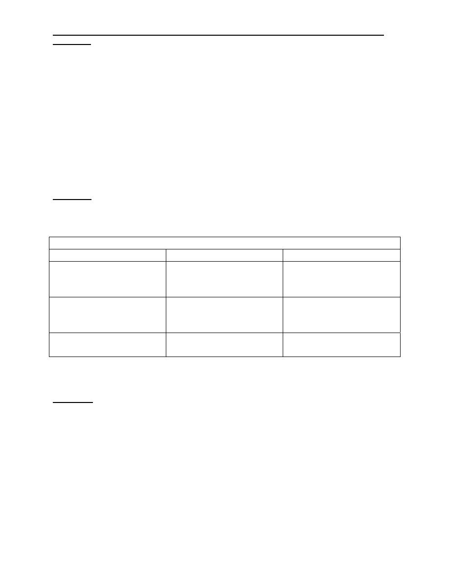
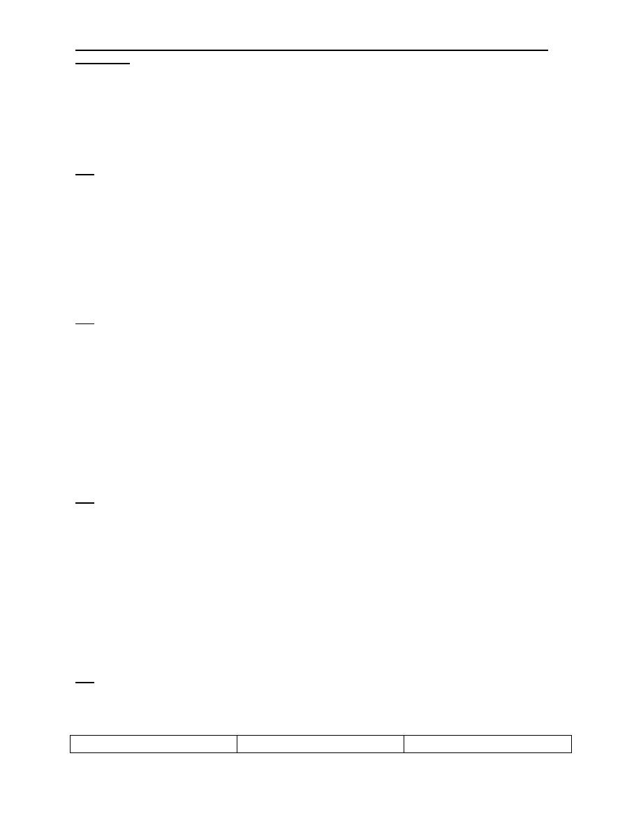
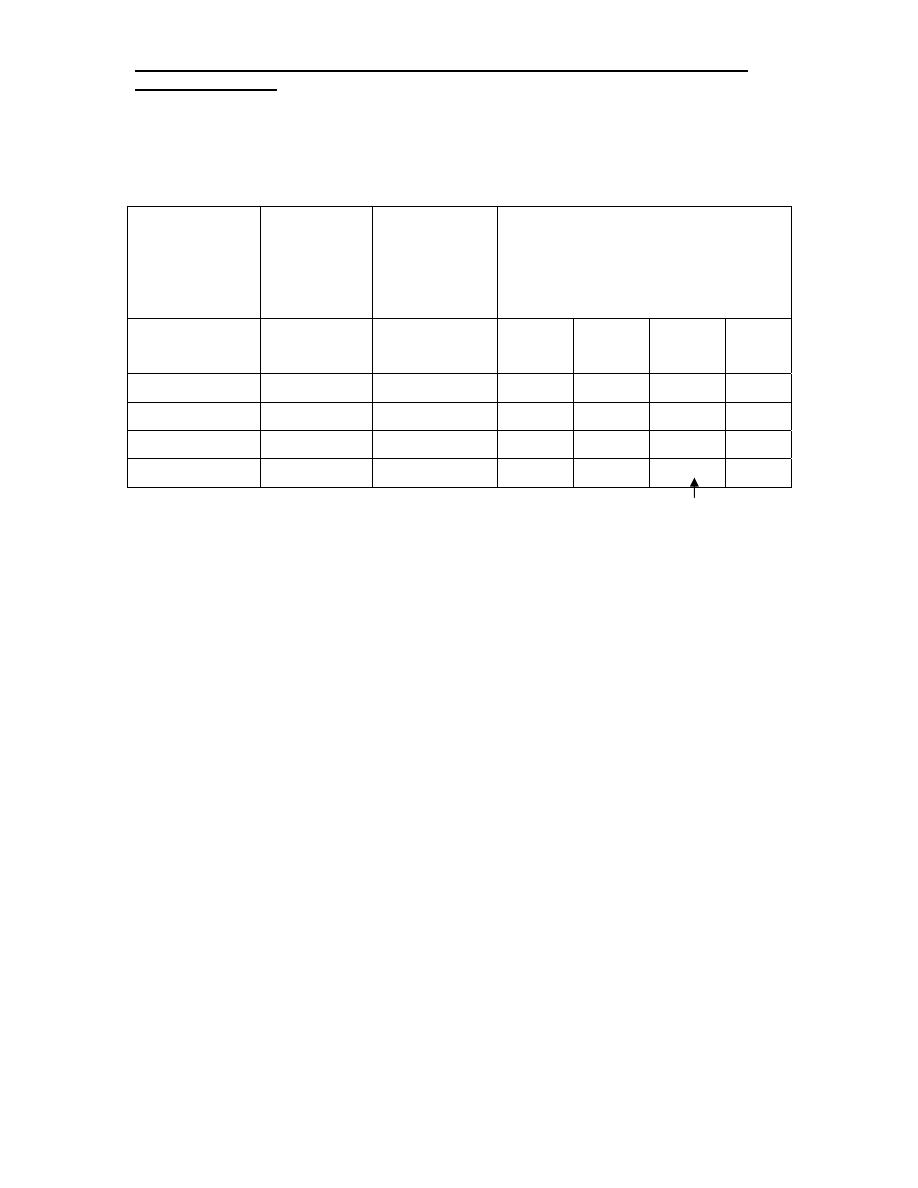
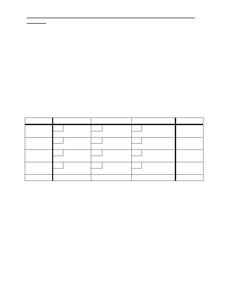
Example: A manager wants to know many units of each product to produce on a
daily basis in order to achieve the highest contribution to profit. Production
requirement for the products are shown in the following table
Production Departments
I II
Processing time required
for the first product
(Hours)
4 2
Processing time required
for the second product
(Hours)
2 4
Production capacity
available (Hours)
60 48
The profit is £8 for each unit of the first product and £6 for each unit of the second
product
Solution:
1- Define the objective. The problem is a maximum problem.
2- Define the decision variables. We need to determine the number of units to
be produced.
Let: X
i
be the number of units of type i (i= 1,2)
Therefore : X
1
= number of units of the first product.
X
2
= number of units of the second product.

Industrial Engineering (IE) - Dr. Khallel Ibrahim
Mahmoud
X
1,
X
2
are the decision variables, when we know their values the problem will be
solved.
3- The objective function for the LP is:
Maximize Z = 8X
1
+6X
2
This means the profit Z depend on how many units (X
1,
X
2
) are manufactured. Z=
c
1
x
1
+ c
2
x
2
where c
1
, c
2
are the respective profits for each type of product. c
1
=£8
c
2
=£6 and Z = 8X
1
+6X
2
and we should select values of the decision variables
X
1,
X
2
that result in the maximum value of Z.
4- There are two constraints :
Maximum production capacity for Dep.I ≤ 60 hours
Maximum production capacity for Dep.II ≤ 48 hours
( Note: because all the constraints in this problem are maximum capacity , all
constraints are the ≤ type)
Now we have to write the coefficient for each decision variable in each constraint.
The two constraints can be expressed as:
4X
1
+2X
2
≤ 60 constraint Dep.I
2X
1
+4X
2
≤ 48 constraint Dep.II
Consider the first constraint ( Dep.I) what is the coefficient of X
1
in this constraint?
It is the processing time (Hours) required per unit of X
1
. In other word, it is the
processing time used in manufacturing each unit, first product, or 2 hours.
Similarly, the coefficient of X
2
in this first constraint is 1 hour.
Therefore the two constraints can be expressed as :
4X
1
+2X
2
≤ 60
2X
1
+4X
2
≤ 48
And the no. negatively restriction is all X
j
≥ 0 , X
1,
X
2
≥ 0

Industrial Engineering (IE) - Dr. Khallel Ibrahim
Mahmoud
Graphical LP solution:
Steps in the graphical method
1- Formulate the objective and constraint functions.
2- Draw a graph with one variable on the horizontal axis and one on the
vertical axis.
3- Plot each of the constraints as if they were lines or equlities.
4- Outline the feasible solution space.
5- Circle the potential solution points .These are the intersections of the
constraints or axes on the inner (minimization) or outer (maximization)
perimeter of the feasible solution space.
6- Substitute each of the potential solution point values of the two decision
variables into the objective function and solve for Z.
7- Select the solution point that optimizes Z.
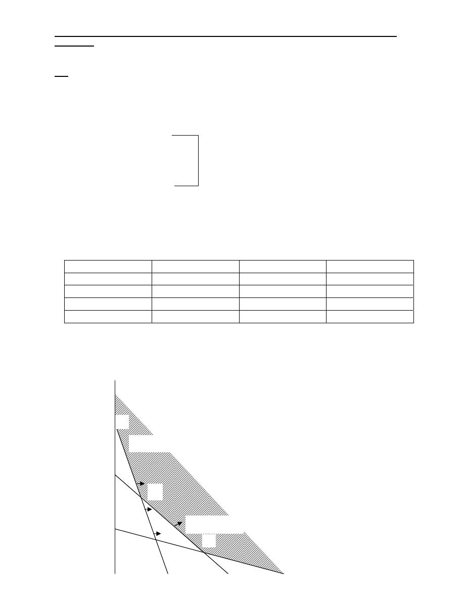
Solution of maximization model
To demonstrate the steps of the graphical solution of a maximization problem we
use the previous example:
Z = 8X
1
+6X
2
Subject to:
4X
1
+2X
2
≤ 60
2X
1
+4X
2
≤ 48
X
1
≥ 0 , X
2
≥ 0
Solution:
1- Plot the constraints (shown in the following figure) change constraints to
equalities:
Industrial Engineering (IE) - Dr. Khallel Ibrahim
Mahmoud
4X
1
+2X
2
≤ 60 4X
1
+2X
2
= 60
2X
1
+4X
2
≤ 48 2X
1
+4X
2
= 48
For each constraint ( set X
1
=0 and solve for X
2
, then set X
2
=0 and solve for X
1
)
the graph the constraint as if it were an equality
4X
1
+2X
2
= 60 X
1
=15 X
2
=0
X
1
=0 X
2
=30
2X
1
+4X
2
= 48 X
1
=24 X
2
=0
X
1
=0 X
2
=12
2- Outline the feasible solution space the values of X
1
and X
2
at points M,A,B
and C are four potential solutions to problem.
Note: point B can be determined as follow:
4X
1
+2X
2
= 60
(2X) 2X
1
+4X
2
= 48
4X
2
+2X
2
= 60
4X
2
+8X
2
= 96
6X
2
=36
X
2
=36/6 = 6
Then: 4X
1
+2X
2
= 60
4X
1
+2(6) = 60
4X
1
= 48
X
1
= 48/4 = 12
Points X
1
X
2
Z
M 0 0
Z=8(0)+6(0)=0
Industrial Engineering (IE) - Dr. Khallel Ibrahim
Mahmoud
A 15 0
Z=8(15)+6(0)=120
B 12 16
Z=8(12)+6(6)=132
C 0 12
Z=8(0)+6(12)=72
To maximize Z, the optimal solution is point B, where X
1
=12 and X
2
=6 and
Z=£132 profit.
B
X
1
A
X
Feasible
solution space
4X
1
+2X
2
≤ 60
2X
1
+4X
2
≤ 48
C
M
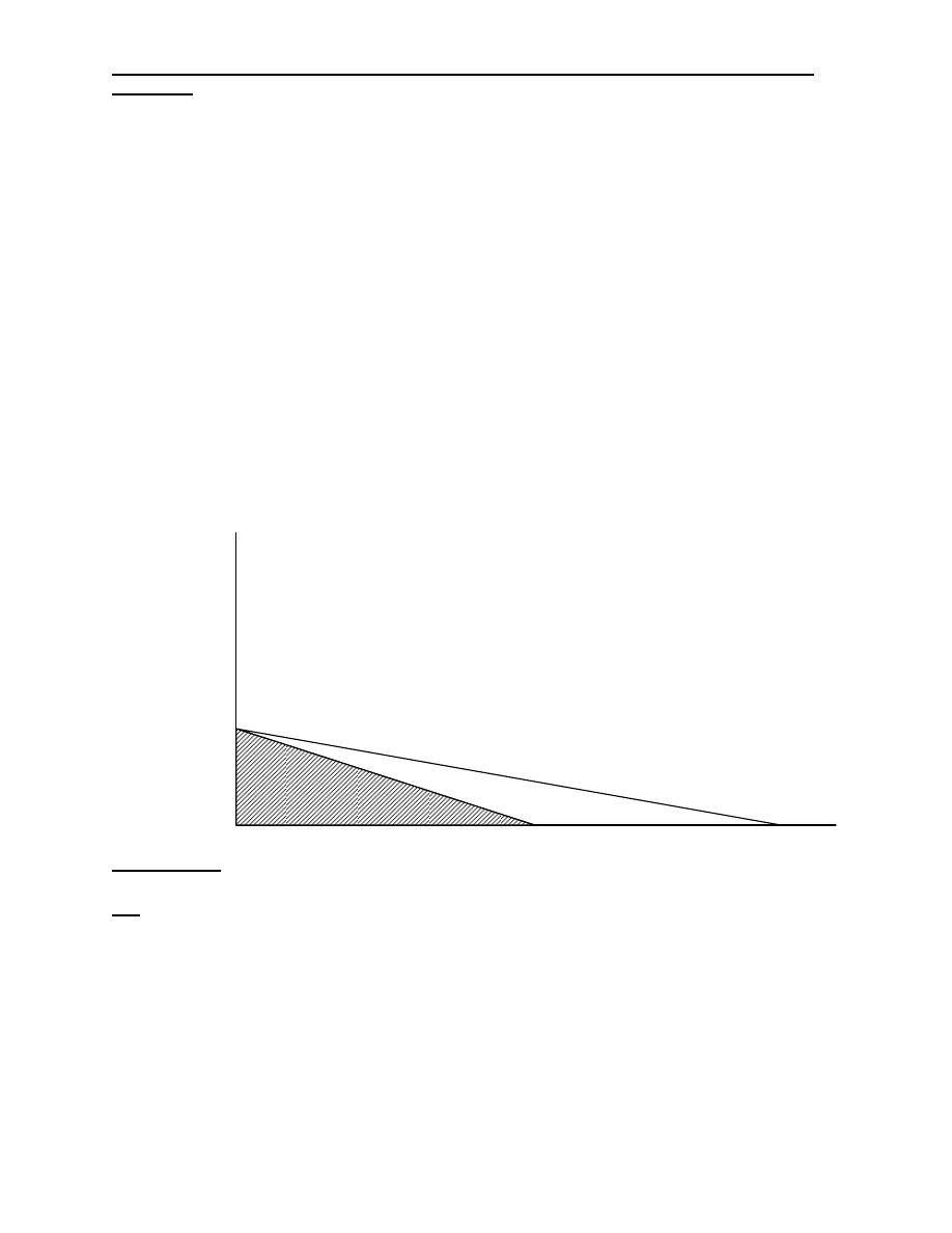
Minimization case:
Consider the following LP problem:
Min Z = 3X
1
+8X
2
Subject to:
X
1
≤ 80
X
2
≥ 60
X
1
+ X
2
=200
X
1
, X2 ≥ 0
Solved problem: X
1
=80 X
2
=60
X
1
=0 X
2
=200
X
1
=200 X
1
=0
Industrial Engineering (IE) - Dr. Khallel Ibrahim
Mahmoud
B/ X
1
+ X
2
=200
X
1
=80
Then X
2
=200-80
=120
Point X
1
X
2
Z
A 0 200
3(0)+8(200)=1600
B 80 120
3(80)+8(120)=1200
Min Z=1200
X
1
=80 X
2
=120
X
2
≥60
X
20
16
12
40
40
80
80
12
16
X
A
X
1
≤80
X
1
+ X
2
=200
B
20
Special cases in LP
Five special cases and difficulties arise at times when using the graphical approach
to solve LP problems:
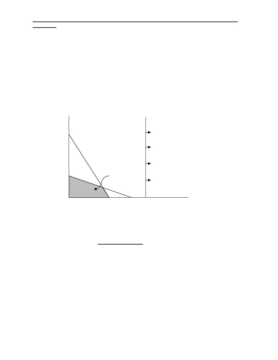
1)
Infeasibility: infeasibility is a condition that arises when
there is no solution to LP problem that satisfies all of constraints given.
Industrial Engineering (IE) - Dr. Khallel Ibrahim
Mahmoud
Graphically, it means that no feasible solution region exists- a situation that
might occur if the problem was formulated with conflicting constraints.
Let us consider the following three constraints: X
1
+2X
2
≥6
2X
1
+X
2
≥8
X
1
≥7
X
Region satisfying
3rd constraint
Region satisfying
first 2 constraints
X
8
6
4
2
8
6
4
2
As seen in the figure there is no feasible solution region for this problem because
of the presence of conflicting constraints.
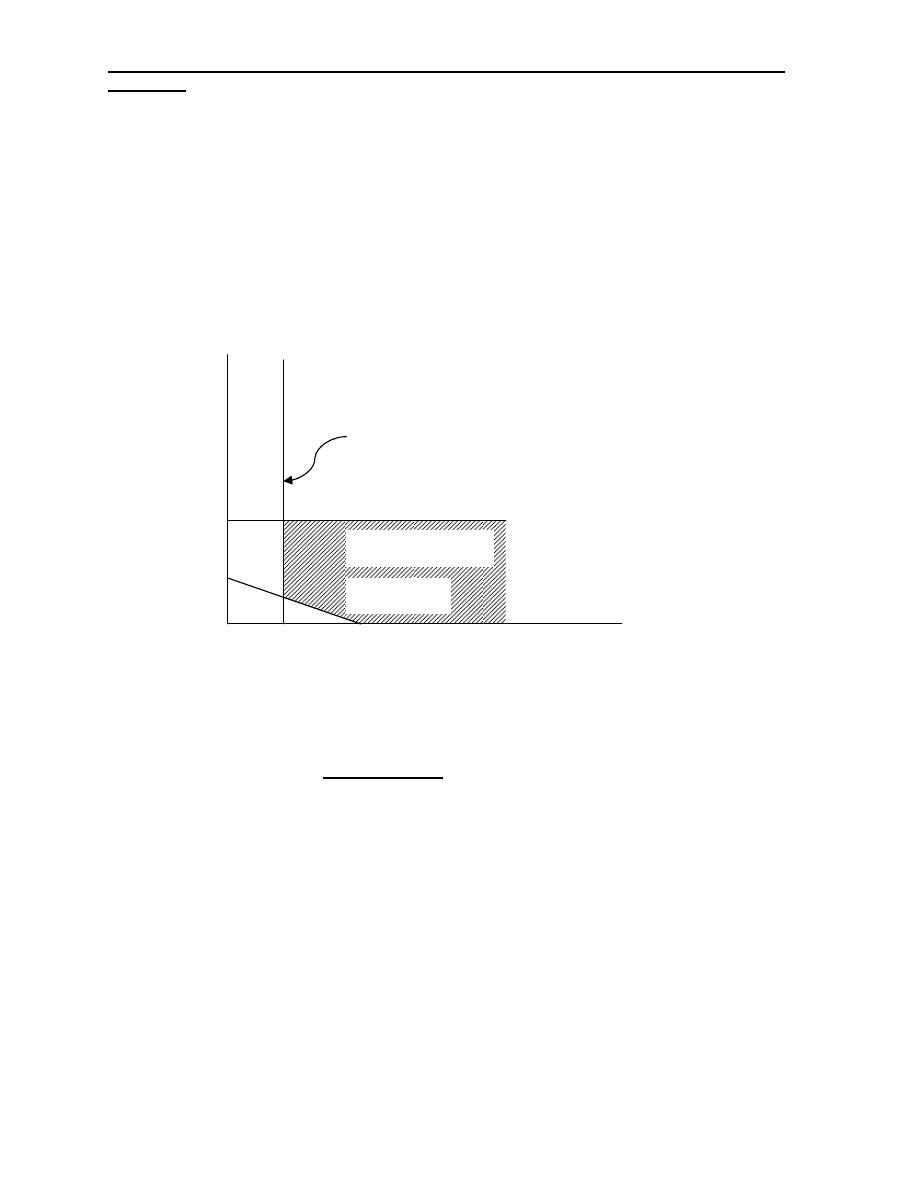
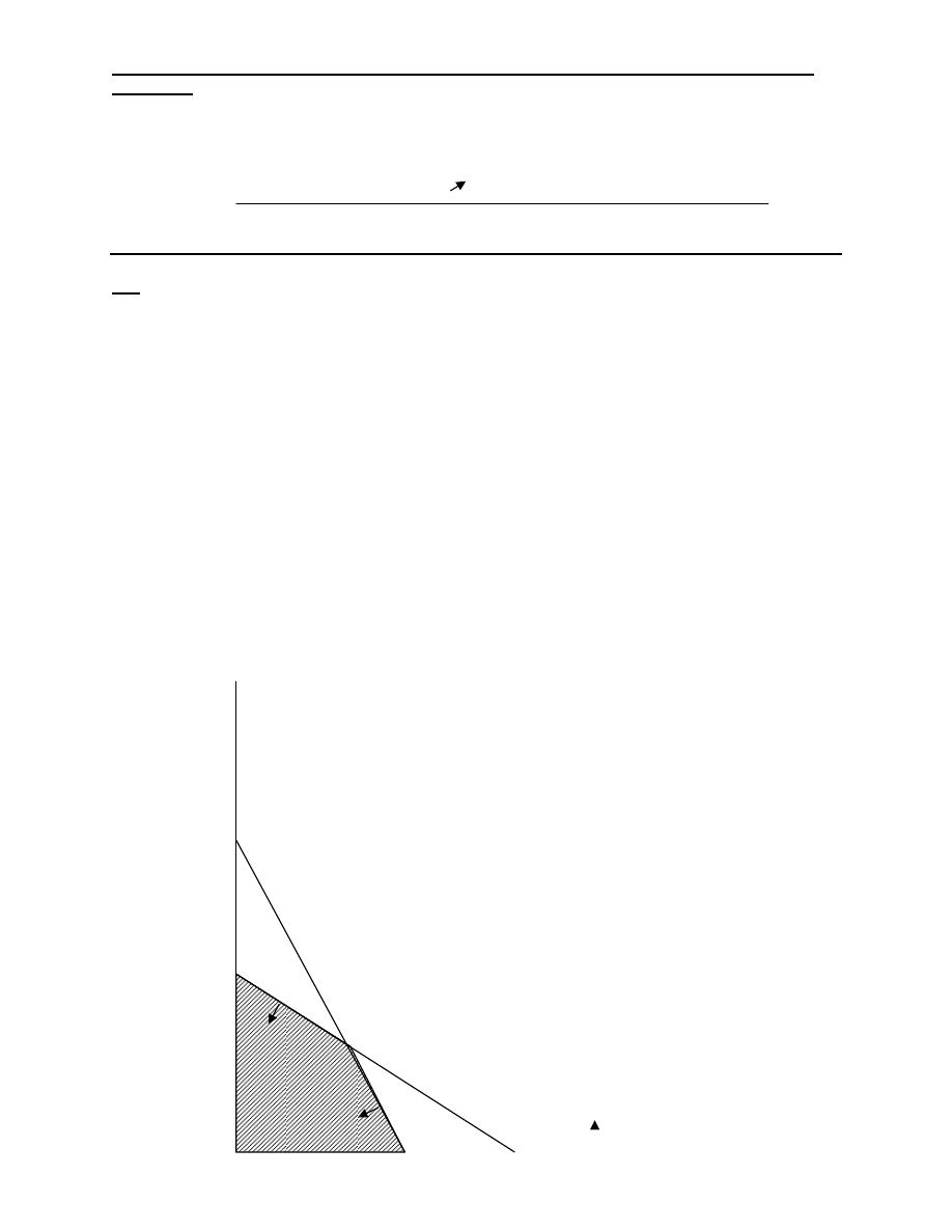
2)
Unboundedness:
Sometimes a linear program will not have a finite solution. This means that in a
maximization problem, for example, one or more solution variables, and the profit,
can be made infinitely large without violating any constraints. If we try to solve
such a problem graphically, we will note that the feasible region is open-ended.
Let us consider a simple example to illustrate the situation.
Z = 3X
1
+5X
2
Subject to: X
1
≥ 5
Industrial Engineering (IE) - Dr. Khallel Ibrahim
Mahmoud
X
2
≤ 10
X
1
+2 X
2
≥10
X
1
, X2 ≥ 0
X
X
2
≤10
Feasible Region
X
1
≥ 5
X
1
+2 X
2
≥10
15
10
5
X
5
10
15
20
As you see, because this is a maximization problem and the feasible region extends
infinitely the right, there is unboundedness or unbounded solution.
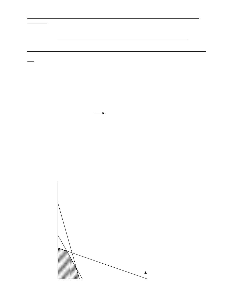
3)
Redundancy: The presence of redundant constraints
occurs in large LP formulations, a redundant constraint is simply on that
does not affect the feasible solution region.
Let us kook at the following example:
Max Z= X
1
+2X
2
Subject to: X
1
+X
2
≤ 20
2X
1
+X
2
≤ 30
X
1
≤ 25
Industrial Engineering (IE) - Dr. Khallel Ibrahim
Mahmoud
X
1
, X2 ≥ 0
X
X
1
≤25
Redundan
t
Feasibl
e
X
1
+ X
2
≤20
2X
1
+ X
2
≤30
X
35
30
25
20
15
10
5
5
10
15
20
25
30
The third constraint, X1≤25 is redundant and unnecessary in the formulation and
solution of the problem because it has no effect on the feasible region set.
4) Alternate Optimal Solutions:
An LP problem may on occasion, have two or more alternate optimal solutions.
Graphically, this is the case when the objective function’s isoprofit or isocost
line runs perfectly parallel to one of the problem’s constraints.
Industrial Engineering (IE) - Dr. Khallel Ibrahim
Mahmoud
Ex: Max Z= 3X
1
+2X
2
Subject to: 6X
1
+4X
2
≤ 24
X
1
≤ 3
X
1
, X2 ≥ 0
1
1
2
2
3
3
4
4
5
5
A
Isoprofit line for
12/line segment AB
6
B
Optimum solutions consists of all
combinations of X
1
,X
2
along the AB
X
Isoprofit
line for 8
X
6
As you see any point along the line between A and B provides an optimal X
1
and X
2
combination Z=12
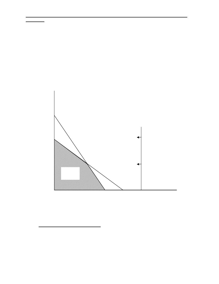
5) Degenercy:
Degenercy is a condition that arises when one of the decision variable equal zero.
Look to the following example:
Industrial Engineering (IE) - Dr. Khallel Ibrahim
Mahmoud
Max Z = 3X
1
+9X
2
Subject to: X
1
+4X
2
≤ 8
X
1
+2X
2
≤ 4
X
1
, X2 ≥ 0
Solution: X
1
=8 X
2
=2
X
1
=4 X
2
=2
Then: at point A
X
1
=0 X
2
=2 Max Z=18
5
X
B
A
4
3
2
1
1
2
3
4
5
6
7
8
Problems:
Q1/ Montana wood products manufacturers two high-quality products, chairs and
bookshelf units. Its profit is $15 per chair and $21 per bookshelf unit. Next week’s
production will be constrained by two limited resources, labor and wood. The labor
available next week is expected to be 920 labor hours, and the amount of wood
available is expected to be 2400 board feet. Each chair requires 4 labor hours and 8
board feet of wood. Each bookshelf unit requires 3 labor hours and 12 board feet of
wood. Management would like to produce at least 100 units of each product.
Industrial Engineering (IE) - Dr. Khallel Ibrahim
Mahmoud
a-
To maximize total profit, how many chairs and bookshelf
units should be produced next week?
b-
How much profit will result?
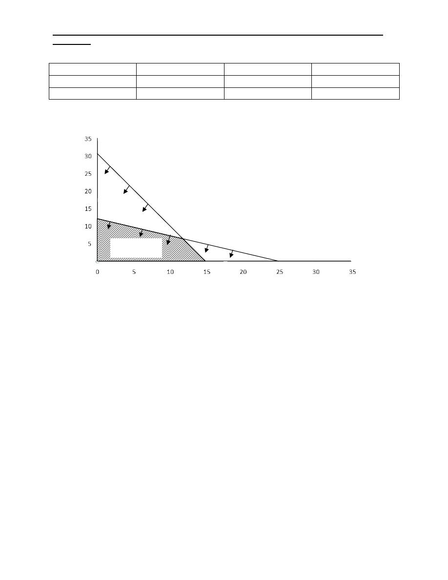
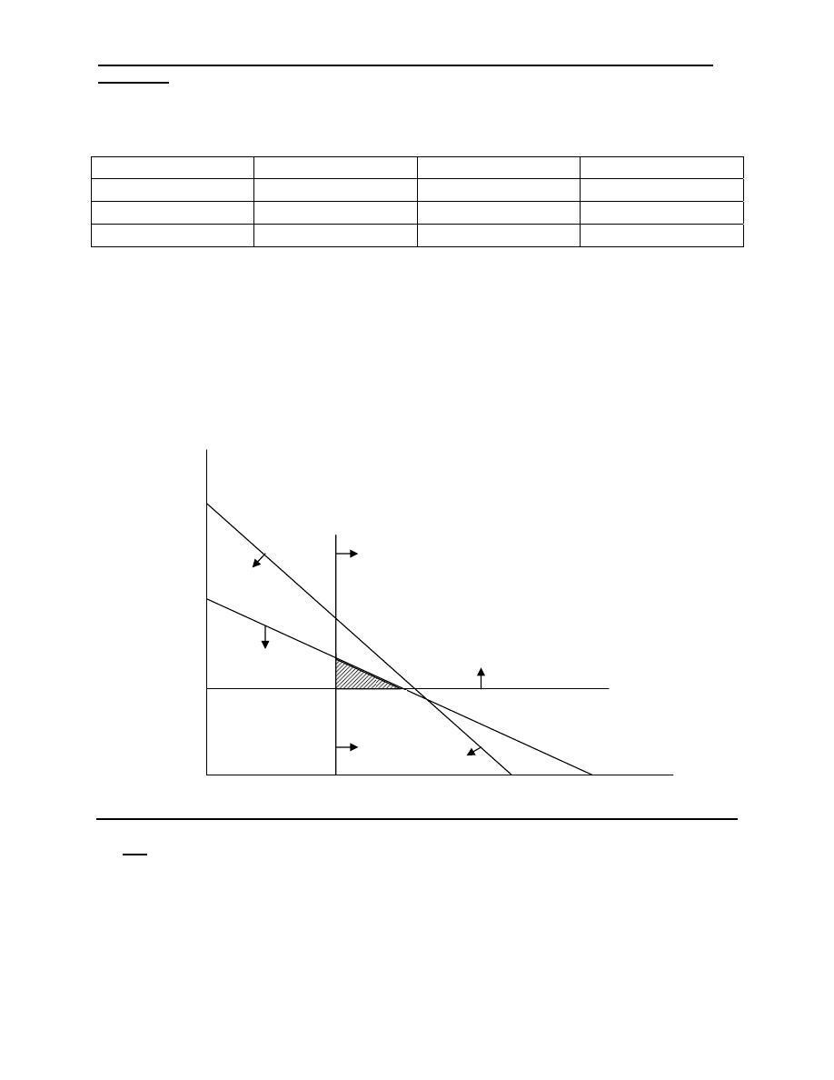
Q2: solve graphically the following linear programming problem:
Max Z = 60X
1
+40X
2
Subject to: 2X
1
+X
2
≤ 60
X
1
≤ 25, X
2
≤ 35
X
1
, X2 ≥ 0
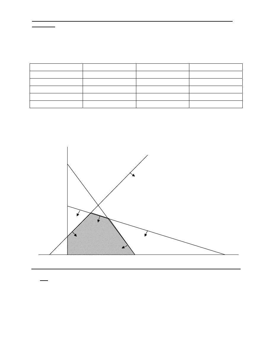
Q3: solve graphically:
Max Z = 10X
1
+15X
2
Subject to: 2X
1
+X
2
≤ 26
2X
1
+4X
2
≤ 56
X
1
-X
2
≥-5
X
1
, X2 ≥ 0
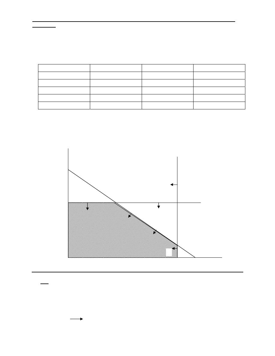
Q4: Consider the following problem and solve graphically:
Minimize Z = 2X
1
+4X
2
Subject to: X
1
+X
2
≤ 14
3X
1
+2X
2
≥ 30
2X
1
+X
2
≤18
X
1
, X2 ≥ 0
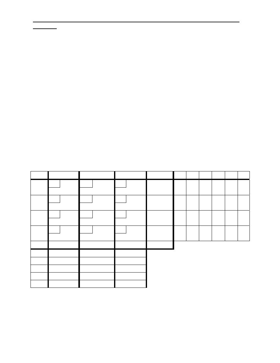
Q5: Tellitell Television company operates two assembly lines, line I and line II.
Each line is used to assemble the components of three types of televisions: colour,
standard and Economy. The expected daily production on each line is as:
TV Model
Line I
Line II
Industrial Engineering (IE) - Dr. Khallel Ibrahim
Mahmoud
Colour 3
1
Standard 1
1
Economy 2
6
The daily running costs for two lines average £6000 for line I and £4000 for line II.
It is given that the company must produce at least 24 colour, 16 standard, and 48
economy TV sets for which an order is pending.
You are required to formulate the above problem as (LP) taking the objective
function as minimization of total cost. Also determine the number of days that the
two lines should be run to meet the requirements.
Q6: Suppose two types of television sets are produced with a profit of 6 units from
each television of type II. In addition 2 and 3 units of raw materials are needed to
produce one television of type I and II respectively. And 4 and 2 units of time are
required to produce one television of type I and II respectively. If 100 units of raw
materials and 120 units of time are available. How many units of each type of
television should be produced to maximize profit?
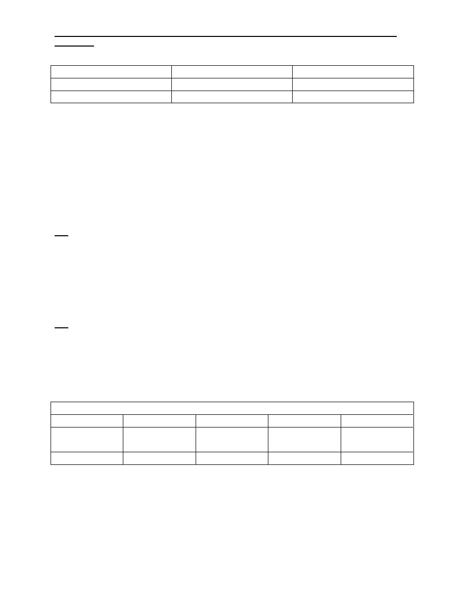
Q7: A wood product firm uses available time at the end of each week to make
goods for stocks. Currently two products on the list of items are produced for
stock: a chopping board and a knife holder. Both items require three operations:
cutting, gluing, and finishing.
The manager of the firm has collected the following data on these products:
Time per unit (minutes)
Item Profit/unit
Cutting Gluing Finishing
Chopping
board
$2 1.4 5 12
Knife
holder
$6 0.8 13 3
The manager has also determine that during each week, 56 minutes are available
for cutting, 650 minutes are available for gluing and 360 minutes are available for
finishing.

Industrial Engineering (IE) - Dr. Khallel Ibrahim
Mahmoud
a-
Determine the optimal quantities of decision variables.
b-
Which resources are not completely used by your solution?
How much of each resource is unused?
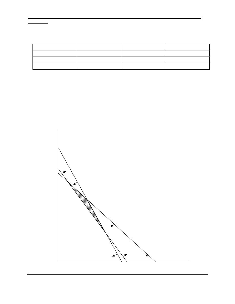
Q8: solve the following problem using graphical linear programming.
Minimize Z = 2X
1
+3X
2
Subject to: 4X
1
+2X
2
≥ 20
2X
1
+6X
2
≥ 18
X
1
+2X
2
≤12
X
1
, X2 ≥ 0
Solutions: Lec. No.2
Q1: Let X
1
: number of chairs to produce next week.
X
2
: number of bookshelves to produce next week.
Max Z = 15X
1
+21X
2
Subject to: 4X
1
+3X
2
≤920 …….. (1)
8X
1
+12X
2
≤ 2400 …….. (2)
X
1
≥100 X
2
≥100
X
1
, X2 ≥ 0
X
1
=0 X
2
=306.6
X
2
=0 X
1
=230 …………….. (1)
X
1
=0 X
2
=200
X
2
=0 X
1
=300 …………… (2)
Z= 4350 with X
1
=150 X
2
=100
Industrial Engineering (IE) - Dr. Khallel Ibrahim
Mahmoud
Point X
1
X
2
Z
A 100 100
3600
B 100
133.3
4299.3
C 150 100
4350
50
10
15
20
25
B
C
A
X
30
350
300
250
20
15
100
50
X
Q2: Max Z = 60X
1
+40X
2
Subject to: 2X
1
+X
2
≤60
X
1
≤25 X
2
≤35
X
1
, X2 ≥ 0
Industrial Engineering (IE) - Dr. Khallel Ibrahim
Mahmoud
X
1
=0 X
2
=306.6
X
2
=0 X
1
=30
Point X
1
X
2
Z
M 0 0 0
A 0 35
1400
B 12.5 35 2150
C 25 10
1900
D 25 0 1500
B: 2X
1
+X
2
= 60 X
2
=35 X
1
= (60-35)/2 = 12.5
It is clear that Z equal to 2150 is Maximum at B when X
1
=12.5 X
2
=35.
X
X
2
≤35
X
1
≤25
C
B
2X
1
+X
2
≤60
D
X
60
50
40
A
30
20
10
M
5
10
15
20
25
30
Q3: Max Z = 10X
1
+15X
2
Subject to: 2X
1
+X
2
≤26
2X
1
+4X
2
≤ 56
X
1
-X
2
≥-5 -X
1
+X
2
≤5
Industrial Engineering (IE) - Dr. Khallel Ibrahim
Mahmoud
X
1
, X2 ≥ 0
X
1
=-5 X
2
=5
Point X
1
X
2
Z
M 0 0 0
A 0 5 75
B 6 11
225
C 8 10
230
D 13 0 130
Hence, Z is Maximum (230) at C.
4
4
8
8
12
12
16
16
18
20
X
-8
-4
M
28
X
A
24
B
2X
1
+4X
2
≤ 56
C
2X
1
+X
2
≤26
-X
1
+X
2
≤5
D
20
24
28
Q4: Min Z = 2X
1
+4X
2
Subject to: X
1
+X
2
≤14
3X
1
+2X
2
≥30
2X
1
+X
2
≤18
Industrial Engineering (IE) - Dr. Khallel Ibrahim
Mahmoud
X
1
, X2 ≥ 0
Point X
1
X
2
Z
A 2 12 52
B 4 10 48
C 6 6 36
Thus, Z is Minimum at point C when X
1
, X
2
=6 Z=36 .
2
2
4
4
6
6
8
8
10
10
12
B
12
14
18
16
X
A
C
X
1
+X
2
≤14
3X
1
+2X
2
≥30
2X
1
+X
2
≤18
14
X
16
18
Industrial Engineering (IE) - Dr. Khallel Ibrahim
Mahmoud
Q5: Let X
1
= the number of days the line I is run.
X
2
= the number of days the line II is run.
Min Z = 6000X
1
+4000X
2
Subject to: 3X
1
+X
2
≥24
X
1
+X
2
≥16 Production Requirement
2X
1
+6X
2
≥48
X
1
, X2 ≥ 0
Point X
1
X
2
Z
A 0 24
96000
B 4 12
72000
C 12 4
88000
D 24 0
144000
Thus, to Minimize cost, line I should be run for 4 days and line II for 12 days.
4
8
12
16
20
B
24
X
1
+X
2
≥16
3X
1
+X
2
≥24
28
X
C
A
Industrial Engineering (IE) - Dr. Khallel Ibrahim
Mahmoud
2X
1
+6X
2
≥48
D
X
4
8
12
16
20
24
Q6: let X
1
: be the number of units of type I produced.
X
2
: be the number of units of type II produced.
Max Z = 6X
1
+4X
2
Subject to: 2X
1
+3X
2
≤100 (raw material time)
4X
1
+2X
2
≤ 120
X
1
, X2 ≥ 0
The optimum solution at point C (X
1
=20, X
2
=30) Hence, 20 units of type I and 20
units of type II should be produced to yield a maximum profit of
Z=6(20)+4(20)=200
10
20
30
40
50
B
60
C
80
D
70
X
2
X
Industrial Engineering (IE) - Dr. Khallel Ibrahim
Mahmoud
A
1
2
30
50
40
70
60
80
Q7: Let board = X
1
holder= X
2
Max = 2X
1
+6X
2
Subject to: 1.4X
1
+0.8X
2
≤56 …………… (1)
5X
1
+13X
2
≤ 650 ………………. (2)
12X
1
+3X
2
≤ 360 ………………. (3)
a) The solution at point A X
1
=0 X
2
=50
Z= 2(0) +6(50) = 300
b) Cutting: 56- 0.8(50) = 15 minutes. (40,0) (0,70) ………… (1)
Gluing: 13X50=650 650-650=0 (130,0) (0,50) …………… (2)
Finishing: 3X50=150 360-150=210 minutes. (30,0) (0,120) ………… (3)
X
20
40
60
80
10
B
120
A
140
C
X

Industrial Engineering (IE) - Dr. Khallel Ibrahim
Mahmoud
D
20
4
60
10
80
14
12
16
Q8: The optimum solution X
1
=4.2 and X
2
=1.6
Minimum Z=2(4.2)+3(1.6) = 13.2

Industrial Engineering (IE) - Dr. Khallel
Ibrahim Mahmoud
Industrial Engineering
(IE)
Dr. Khallel Ibrahim Mahmoud
University of Technology
Electro-mechanical Engineering Dept.
Lec.
N
o
(3)
Linear Programming
Model
Simplex Method
2011

Industrial Engineering (IE) - Dr. Khallel
Ibrahim Mahmoud
Simplex Method
The linear programming situation with two decision variables
is easy tackled by a graphical method of solution. However
most practical linear programming problem contain more
than two decision variables. Graphic representation is
difficult (three dimensional) and requires more time for the
determination of an optimal solution. The solution method in
such cases is the simplex method. The simplex method is an
iterative procedure that consists of moving from one basic
feasible solution to another in such a way that the value of
the objective function does not decrease (in the
maximization problem). This process continue until an
optimal solution is reached, if one exist.
The steps required to solve the problem – maximizing
are:
Step 1
: Define the problem in standard form. This indicates
the construction of a linear programming model.
Step 2
: convert the inequalities into equation by insert slack
variables.
Step 3
: Construct a matrix of the coefficients of these
equations.
Step 4
: This step amends the previous feasible solution so
as to improve the profit.
The simplex method will be illustrated with the following
example.

Industrial Engineering (IE) - Dr. Khallel
Ibrahim Mahmoud
Example
/ Consider the following LP:
Maximize Z= 6X
1
+8X
2
Subject to:
2X
1
+5X
2
≤ 40
8X
1
+4X
2
≤ 80
X
1
,X
2
≥ 0
Step 1
/ Conversion of inequalities into equations Add slack
variables to remove inequalities
2X
1
+5X
2
+S
1
= 40
8X
1
+4X
2
+ S
2
= 80
Where S
1
,S
2
slack variables (surplus) putting X
1
=0 and X
2
=0 we get
S
1
= 40 , S
2
= 80
Max Z =6X
1
+8X
2
+oS
1
+ oS
2
Subject to:
2X
1
+5X
2
+S
1
+ oS
2
= 40
8X
1
+4X
2
+ oS
1
+ S
2
= 80
Industrial Engineering (IE) - Dr. Khallel
Ibrahim Mahmoud
Step 2/
Construct the simplex tableau. The standard form
can be summarized in a compact tableau form as:
Coefficient
of OF
variables
in basis
Basic
variables
Values of
basic
variables
Coefficient of OF
variables
(Cj)
( Cj)
(A)
(q)
6
X
1
8
X
2
0
S
1
0
S
2
0 S
1
40 2
5
1
0
0 S
2
80 8
4
0
1
Zj 0
0
0
0
0
Cj-Zj 6
8
0
0
Initial solution: X
1
= 0
X
2
= 0
S
1
= 40
S
2
= 80
Z = 0
Zj:
Zj (q) = 40(0) + 80(0) = 0
Zj (X
1
) = 2(0) + 8(0) = 0
Zj (X
2
) = 5(0) + 4(0) = 0
Zj (S
1
) = 1(0) + 0(0) = 0
Zj (S
2
) = 0(0) + 1(0) = 0
Cj – Zj :
Industrial Engineering (IE) - Dr. Khallel
Ibrahim Mahmoud
(Cj – Zj) X
1
= 6-0 =6 , (Cj – Zj) S
1
= 0-0 =0
(Cj – Zj) X
2
= 8-0 =8 , (Cj – Zj) S
2
= 0
Step 3/
identify the pivot column
X
2
has max positive value (8) Thus the entering variable will
be X
2
in the new solution
Step 4/
identify the pivot row
,
, the smallest value = 8
Thus, S
1
, is the leaving variable. Replacing the leaving
variable S
1
with the entering variable X
2
produces the new
basic solution (X
2
, S
2
) and the pivot element = 5
Types:
1. Pivot row : new pivot row = current pivot row ÷ pivot
element
2. All other rows , including Z:
new row = (Current row) – (its pivot column
coefficient)X(new pivot row)
Type 1
: computation is divide the pivot row (S
1
– row) by the
pivot element (5) .Thus the new row:
Industrial Engineering (IE) - Dr. Khallel
Ibrahim Mahmoud
Type 2
: Computation is applied to the remaining row (S
2
-
row) as follow:
80 – (4X8) = 48
8 – (4X 2/5) = 32/5
4- (4X1) = 0
0 – (4X1/5) = -4/5
1 – (4X0) = 1
The new tableau corresponding to the new basic solution
(X
2
,S
2
) thus becomes:
( Cj)
(A)
(q)
6
X
1
8
X
2
0
S
1
0
S
2
8 X
2
8
1
0
0 S
2
48
0
1
Zj
64
8
0
Cj-Zj
0
0
Observe that the new tableau yields the new basic solution
(X
2
=8 , S
2
= 48 ) with the new value of Z = 64 . An
examination of the last tableau shows that it is not optimal
solution because the variable X
1
has a positive coefficient in
the (Cj-Zj) row ( )
Industrial Engineering (IE) - Dr. Khallel
Ibrahim Mahmoud
An increase in X
1
is advantageous because it will increase
the value of Z. Thus , X
1
is the entering variable.
Next, we determine the leaving variables as follow :
8 ÷ = 20 , 48 ÷ = , Thus the pivot element =
S
2
is the leaving variable , X
1
is the entering variable . and
the new pivot row :
48 ÷ = , ÷ = 1 , 0 ,
÷ =
new X
2
– row : 8- ( X )= 5
- ( X 1) = 0
1- ( X0 ) = 1
- ( X ) =
These Computations produce the following tableau:
( Cj)
(A)
(q)
6
X
1
8
X
2
0
S
1
0
S
2
8 X
2
5 0
1
6 S
2
1 0
Zj
85 6
8
Cj-Zj 0 0
Industrial Engineering (IE) - Dr. Khallel
Ibrahim Mahmoud
Since none of the C
j
-Z
j
row coefficient associated with the
basic variables is positive , the last tableau is optimal.
The optimum solution can be read from the simplex tableau
in the following manner
Decision variables
Optimum value
X
1
15/2 = 7.5
X
2
5
Z 85
The M- Method ( Big – M)
In the previous example , starting the simplex iterations at a
basic feasible . For the LP
s
in which all the constraints are of
the (≤) type, the stacks offer a convenient starting basic
feasible solution. A natural question then arises : How can
we find a starting basic solution for models that involve (=)
and (≥) constraints?
The most common procedure for starting LP
s
that do not
have convenient slacks is to use artificial variables and the
closely related method is proposed for effecting this result :
the M-Method (Big- M).
The M-Method starts with the LP
in the standard form. For
any equation (i) that does not have a slack , we augment an
artificial variable (A
i
) and assign them a penalty in the
objective function to force them to zero level at a later
iteration of the simplex algorithm.

Industrial Engineering (IE) - Dr. Khallel
Ibrahim Mahmoud
Given M is a sufficiently large positive value, the variable A
i
is penalized in the objective function using -MA
i
in the case
of maximization and +MA
i
in the case of minimization.
The following example provides the details of the method:
Min Z = 3X
1
+ 8X
2
Subj. to:
X
1
≤ 80, X
2
≥ 60 , X
1
+ X
2
= 200 , X
1
, X
2
≥ 0
Step1
/ for convenient inequalities into equalities:
X
1
+ S
1
= 80
X
2
- S
2
= 60
X
1
+ X
2
= 200
Putting X
1
, X
2
= 0 we get S
1
= 80 S
2
=- 60
Therefore, we introduce artificial variables and the above
constraints can be written as:
X
1
+ S
1
= 80
X
2
- S
2
+ A
1
= 60
X
1
+ X
2
+ A
2
= 200 A
1
, A
2
Artificial variables
Now addition of this artificial variable destroy the equality
required by the L.p model . Therefore, A
1
, A
2
must not
appear in the final solution . To achieve this it is assigned a
very large penalty (TM) since Z is to be minimized in the
objective function . Therefore we get:
X
1
+ S
1
+0S
2
+0A
1
+0A
2
= 80
Industrial Engineering (IE) - Dr. Khallel
Ibrahim Mahmoud
X
2
+ 0S
1
-S
2
+A
1
+0A
2
= 60
X
1
+ X
2
+0S
1
+0S
2
+0A
1
+A
2
= 200
Min Z = 3X
1
+ 8X
2
+0S
1
+0S
2
+MA
1
+MA
2
( Cj)
(A)
(q)
3
X
1
8
X
2
0
S
1
0
S
2
M
A
1
M
A
2
0 S
2
80 1 0 1
0
0
0
M A
1
60 0 1 0
-1
1
0
A
2
200 1 1 0 0
0
1
M Z
260M
M
2M
0
-M
M
M
Cj-
Zj
3-M
8-2M
0
M
0
0
Step 2
/ identify the pivot column:
This is done by selecting the none basic variable having the
largest negative value in Cj-Zj .
When all the elements in the Cj-Zj row are positive or zero
the optimal solution is reached .
Step3
/ identify the pivot row:
80/0 = 0 , 60/1 = 60 , 200/1 = 200
Pivot = 1 A
1
X
1
X
2
/ 60/1 , 0 , 1/1 , 0 , -1/1 , 1, 0
Row S
1
: will be remain , Row A
2
/200-(1X60) = 140
1- (1X0) = 1
1-( 1X1) = 0
0- (1X0) = 0
Industrial Engineering (IE) - Dr. Khallel
Ibrahim Mahmoud
0-(1X-1) = 1
0-(1X1) = -1
1-(1X0) = 1
( Cj)
(A)
(q)
3
X
1
8
X
2
0
S
1
0
S
2
M
A
1
M
A
2
0 S
1
80 1 0 1
0
0
0
8 X
2
60 0 1 0
-1
1
0
M A
2
140 1 0 0 1
-1
1
Zj
480+
140M
M 8 0
M-8
8-M
M
Cj-
Zj
3-M
0 0
8-M
2M-
8
0
As Cj-Zj is positive under same column the current basic
feasible solution is not optimal and needs to be improved .
Step4
/ Identify the pivot row after identify the pivot column
80/1 = 80 , 1 , 0 , 1 , 0 , 0 , 0
Row X
2
will remain
Row A
2
: 140 – (1X80) = 60
1- (1X1) = 0
0 – (1X0) = 0
0 – (1X1) = -1
1 – (1X0) = 1
-1 – (1X0) = -1
1 – (1X0) = 1
Industrial Engineering (IE) - Dr. Khallel
Ibrahim Mahmoud
Step5
/ create the new tableau
( Cj)
(A)
(q)
3
X
1
8
X
2
0
S
1
0
S
2
M
A
1
M
A
2
3 X
1
80 1 0 1
0
0
0
8 X
2
60 0 1 0
-1
1
0
M A
2
60 0 0
-1
1
-1
1
Zj
720+
60M
3 8
3-M
M-8
8-M
M
Cj-
Zj
0
0
M-3
8-M
2M-
8
0
As Cj-Zj is positive under same column the current solution
is not optimal and need to improve.
Step6
/ identify the pivot column , and pivot row.
80/0 , 60/-1 , 60/1 = 60 A
2
S
1
S
2
: 60 , 0 , 0 , -1 , 1 , -1 , 1
Row X
1
: will be remain
Row X
2
:60- (-1X60) = 120
0- (-1X0) = 0
1- ( -1X0) = 1
0- (-1X-1) = -1
-1 – (-1X1) = 0
1- (-1X-1) = 0
Industrial Engineering (IE) - Dr. Khallel
Ibrahim Mahmoud
0 – (-1X1) = 1
( Cj)
(A)
(q)
3
X
1
8
X
2
0
S
1
0
S
2
M
A
1
M
A
2
3 X
1
80 1 0 1
0
0
0
8 X
2
120 0 1 -1
0
0
1
0 S
2
60 0 0
-1
1
-1
1
Zj
1200
3
8
-5
0
0
8
Cj-
Zj
0
0
5
0
M
M-
8
As Cj-Zj is either positive or zero under all column, the
solution is an optimal solution.
X
1
= 80 , X
2
= 120 , S
2
= 60 , Z= 1200
Industrial Engineering (IE) - Dr. Khallel Ibrahim
Mahmoud
Industrial Engineering (IE)
Dr. Khallel Ibrahim Mahmoud
University of Technology
Electro-mechanical Engineering Dept.
Lec.N
o(4)
The Dual Model
The assignment model
2011

Industrial Engineering (IE) - Dr. Khallel Ibrahim
Mahmoud
The dual Problem
The LP model we develop for a situation is referred to as the primal problem. The
dual problem is a close relates mathematical definition that can be derived directly
from the primal problem.
Consider a linear programming problem concerned with the maximization of an
objective function Z with n decision variables and M constraints (primal). The dual
this problem is concerned with minimization of the value of the objective function
Ź with M decision variables and n constraints. Thus a maximization problem
becomes minimization in the dual and vice verse.
In the mathematical form the primal can be stated as:
Max Z= C
1
X
1
+ C
2
X
2
+ ………. +C
n
X
n
Subject to:
a
11
x
1
+a
12
x
2
+ ……………….. + a
1n
x
n
≤ b
1
a
21
x
1
+a
22
x
2
+ ……………….. + a
2n
x
n
≤ b
2
a
m1
x
1
+a
m2
x
2
+ ……………….. + a
mn
x
n
≤ b
m
X
1
≥ 0 X
2
≥ 0 ………… X
n
≥ 0
The dual of this problem may be expressed in the following form:
Min Ź= b
1
y
1
+ b
2
y
2
+ ………. +b
m
y
m
Subject to:
a
11
y
1
+a
12
y
2
+ ……………….. + a
m1
y
n
≥ c
1
a
12
y
1
+a
22
y
2
+ ……………….. + a
m2
y
m
≥ c
2

Industrial Engineering (IE) - Dr. Khallel Ibrahim
Mahmoud
a
1m
y
1
+a
2n
y
2
+ ……………….. + a
mn
y
m
≥c
n
y
1
≥ 0 y
2
≥ 0 ………… y
m
≥ 0
the variables and constraints of the dual problem can be constructed symmetrically
from the primal problem as follows:
1- A dual variable is defined for each of the m primal constraint equations.
2- A dual constraint is defined for each primal of the n primal variables.
3- The left-hand-side coefficients of the dual constraint equal the constraint
(column) coefficient of the associated primal variable. Its right – hand side
equals the objective coefficient of the same primal variable.
4- The objective coefficient of the dual equal the right- hand side of the primal
constraint equations.
The following examples demonstrate the implementation of these rules.
Ex/ Consider the primal model:
Max Z =6X
1
+ 8X
2
St.to: 2X
1
+5X
2
≤40
8X
1
+4X
2
≤80
X
1 ,
X
2
≥ 0
The dual of this problem as:
Min Ź = 40Y
1
+80Y
2
St. to: 2Y
1
+8Y
2
≥6
5Y
1
+4Y
2
≥8
Y
1
, Y
2
≥ 0
The solution of the dual problem can be obtained by using simplex minimization
procedures.
Min Z = 40 Y
1
+80 Y
2
+oS
1
+oS
2
+MA
1
+MA
2
Industrial Engineering (IE) - Dr. Khallel Ibrahim
Mahmoud
Subject to: 2y
1
+8y
2
- s
1
+A
1
= 6
5y
1
+ 4y
2
- s
2
+ A
2
= 8
40 80 0 0 M M
C
j
A q
Y
1
Y
2
S
1
S
2
A
1
A
2
M A
1
6 2 8 -1 0 1 0
M A
2
8 5 4 0 -1 0 1
Z
j
14M 7M 12M -M -M M
M
C
j
-Z
j
40-7M
80-12M
M M 0
0
80 Y
2
¾ ¼ 1 -1/8 0 1/8 0
M A
2
5 4 0 ½ -1
-1/2 1
Z
j
60+5M 20+4M
80
1/2M-10
-M 10-1/2M
M
C
j
-Z
j
20-4M 0 10-1/2M
M
1/2M-10 0
80 Y
2
7/16 0 1 -5/32
1/16
5/32 -1/16
40 Y
1
5/4 1 0 1/8
-1/4
-1/8 1/4
Z
j
85 40 80 -7.5 -5 7.5 5
C
j
-Z
j
0 0 7.5
5
M-7.5
M-5
ﺣﻞ اﻟﻨﻤﻮذج اﻷوﻟﻲ
)
primal
(
آﺎن آﻤﺎ ﻳﻠﻲ
:
6 8 0 0
C
j
A q
X
1
X
2
S
1
S
2
8 X
2
5 0 1 ¼ -1/16
6 X
1
7.5
1 0 -1/8
5/32
Z
j
85 6 8 5/4
7/16
C
j
-Z
j
0 0 -5/4
-7/16
Dual Primal
S
1
= 7.5
X
1
= 7.5
S
2
= 5
X
2
= 5
Y
1
= 5/4
S
1
= 5/4
Y
2
= 7/16
S
2
= 7/16
Ź = 85
Z = 85
Ex1/ Obtain the dual of the following LP:
Max Z =5X
1
+ 10X
2
+8X
3
St.to: 3X
1
+ 5X
2
+2X
3
≤60

Industrial Engineering (IE) - Dr. Khallel Ibrahim
Mahmoud
4X
1
+ 4X
2
+4X
3
≤72
2X
1
+ 4X
2
+5X
3
≤100
X
1 ,
X
2
,X
3
≥ 0
Solution: Min Ź = 60Y
1
+72Y
2
+100Y
3
St. to: 3Y
1
+4Y
2
+2Y
3
≥5
5Y
1
+4Y
2
+4Y
3
≥10
2Y
1
+4Y
2
+5Y
3
≥8
Y
1
, Y
2
, Y
3
≥ 0
Ex2/ Consider the following LP and write the associated dual problem:
Max Z =7X
1
+ 5X
2
St.to: 3X
1
+X
2
≤48
2X
1
+X
2
≤40
X
1 ,
X
2
≥ 0
Min Ź = 48Y
1
+40Y
2
St. to: 3Y
1
+2Y
2
≥7
Y
1
+Y
2
≥5
Y
1
, Y
2
≥ 0
Ex3/ Write the dual for each of the following primal problem:
Max Z =10X
1
+ 12X
2
St.to: X
1
+X
2
≥15
X
1
= 6
X
2
≤ 8

Industrial Engineering (IE) - Dr. Khallel Ibrahim
Mahmoud
Solution: X
1
+X
2
≥15
X
1
≤ 6 -X
1
≥ -6
X
1
≥6
X
2
≤ 8 -X
2
≥-8
Min Z = 10X
1
+ 12X
2
Sub. To: X
1
+X
2
≥15
X
1
≥6
-X
1
≥ -6
-X
2
≥-8
X
1 ,
X
2
≥ 0
Thus, the dual : Max Ź = 15Y
1
+6Y
2
-6Y
3
- 8Y
4
St. to: 3Y
1
+4Y
2
+2Y
3
≥5
Y
1
+Y
2
-Y
3
≤10
Y
1
-Y
4
≤12
Problems
Write the dual for each of the following problems:
1) Min Z = 10X
1
+ 16X
2
Sub. To: X
1
+X
2
=100
X
1
≤800
X
2
≥400
2) Min Z = 3X
1
+ 8X
2
Sub. To: X
1
+X
2
=200
Industrial Engineering (IE) - Dr. Khallel Ibrahim
Mahmoud
X
1
≤80
X
2
≥60
3) Max Z = 23X
1
+ 32X
2
Sub. To: 10X
1
+6X
2
≤2500
5X
1
+10X
2
≤2000
X
1
+2X
2
≤500
4) Write the primal problem for the following:
Min Ź = 60Y
1
+72Y
2
+100Y
3
St. to: 3Y
1
+4Y
2
+2Y
3
≥5
5Y
1
+4Y
2
+4Y
3
≥10
2Y
1
+4Y
2
+5Y
3
≥8
Y
1
, Y
2
, Y
3
≥ 0
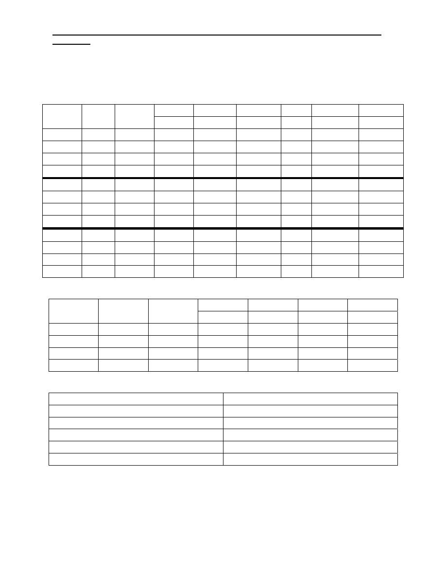
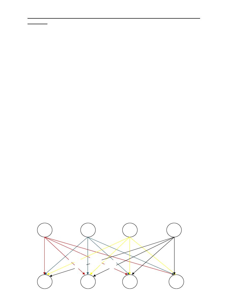
The assignment model
Suppose a company has M jobs that must be completed and it has at least n
workers who can perform any of the M jobs but possibly in a different amount of
time. Which worker should be assigned to each job to minimize the overall time to
complete all M jobs, if each worker is assigned to one and only one job. This is the
classical assignment problem.
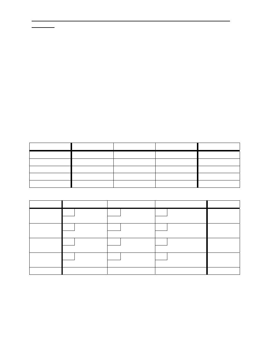
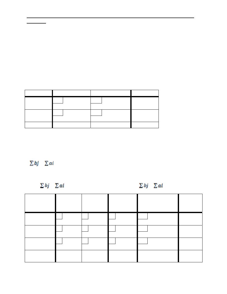
The general assignment model with n workers and M jobs is represented in the
following matrix:
jobs
1 2 M b
j
1
2
n
C
11
C
21
C
n1
C
12
C
22
C
n2
C
1m
C
2m
C
nm
1
1
1
workers
ai 1 1 1
Industrial Engineering (IE) - Dr. Khallel Ibrahim
Mahmoud
The element C
ij
represents the cost of assigning worker i to job j (i= 1,2,…..,n)
(j= 1,1,…..,m).
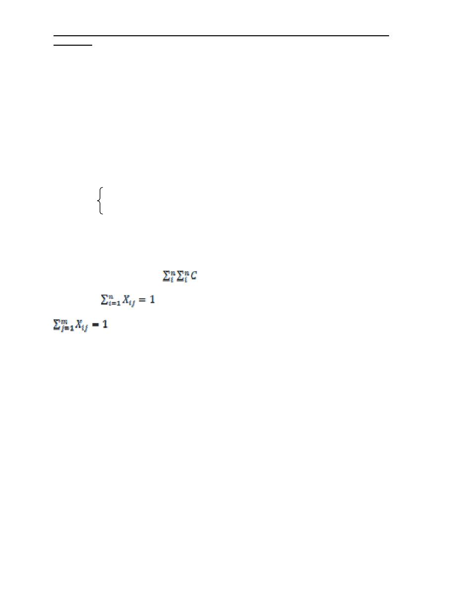
If we let:
X
ij
= 0 if worker i is not assigned to job j
1 if worker i is assigned to job j
C
ij
= efficiency associated with assigning worker i to job j.
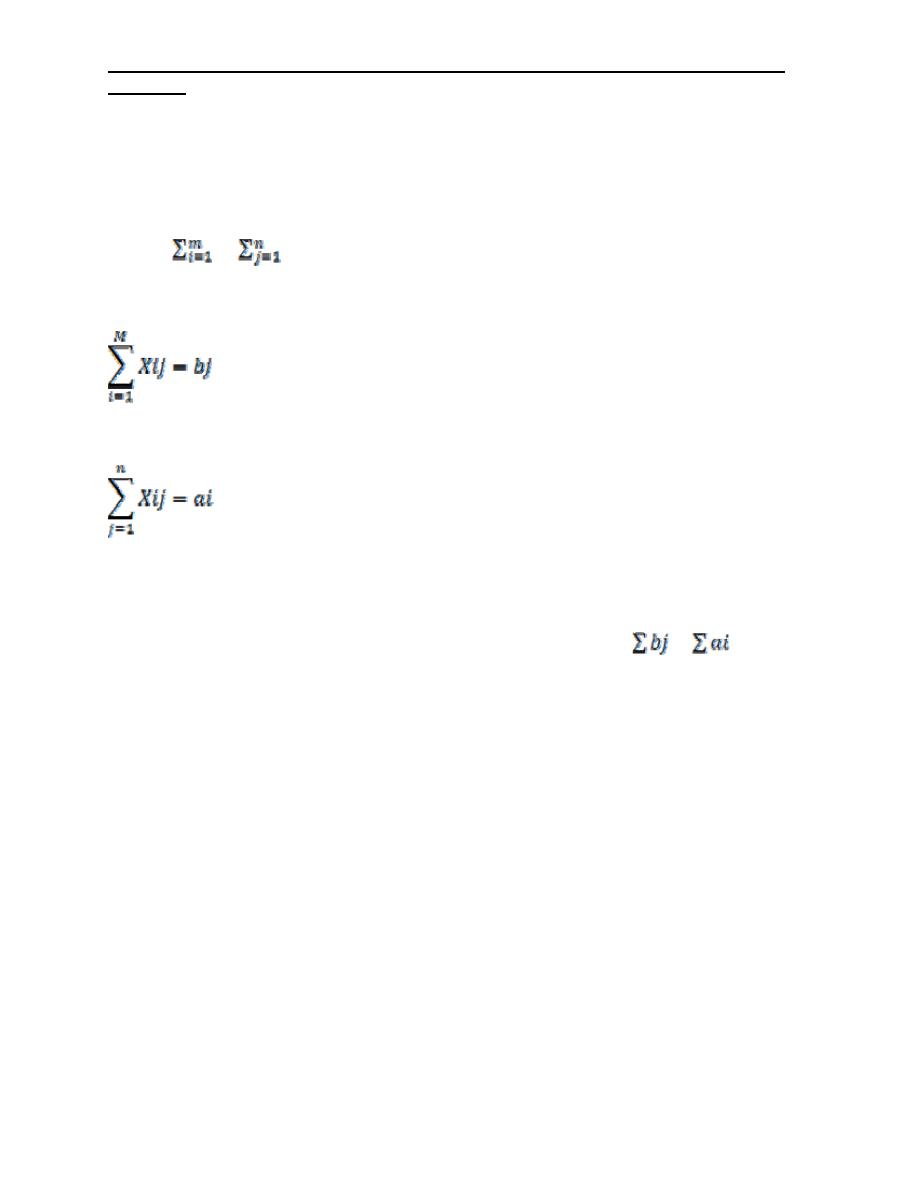
Then mathematically the assignment problem can be stated as:
Minimize (maximize): Z=
ij
X
ij
Subject to:
for j= 1,2,………, m
for i= 1,2,………, n
X
ij
= 0 or 1 for al i and j
The following is a step by step algorithm that uses the Hungarian method to solve
the general assignment problem.
Step 1: for the original cost matrix, identify each row’s minimum, and subtract it
from all the entries of the row.
Step 2: For the matrix resulting from step 1, identify each column’s minimum, and
subtract it from all the entries of the column.
Step 3: Draw the minimum number of horizontal and vertical lines in the last
reduced matrix that will cover all the zero entries. If the number is equal the
columns or rows the feasible assignment can be found, otherwise go to step 4.
Industrial Engineering (IE) - Dr. Khallel Ibrahim
Mahmoud
Step 4: Select the smallest uncover element, and subtract it from every uncovered
element, then add it to every element at the intersection of two lines. And repeat
step 3 until the feasible assignment found.
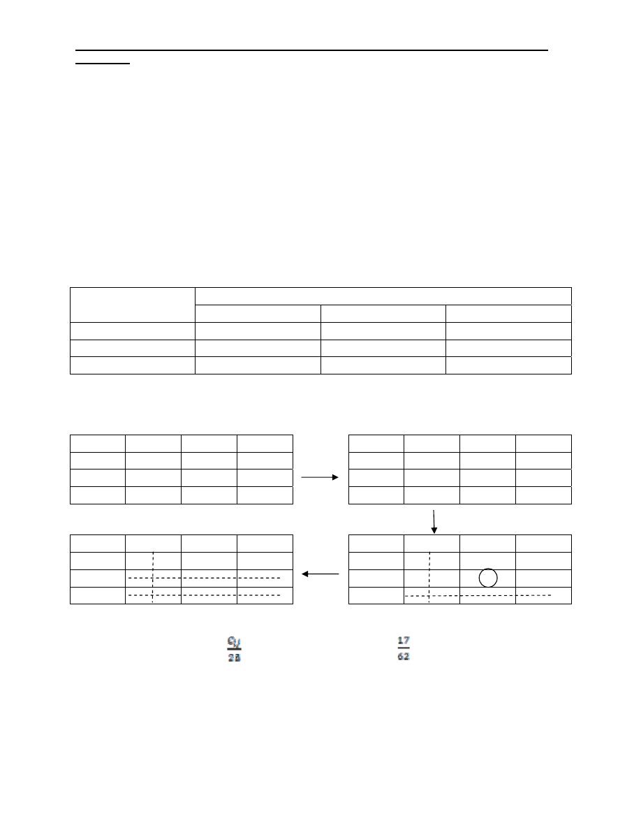
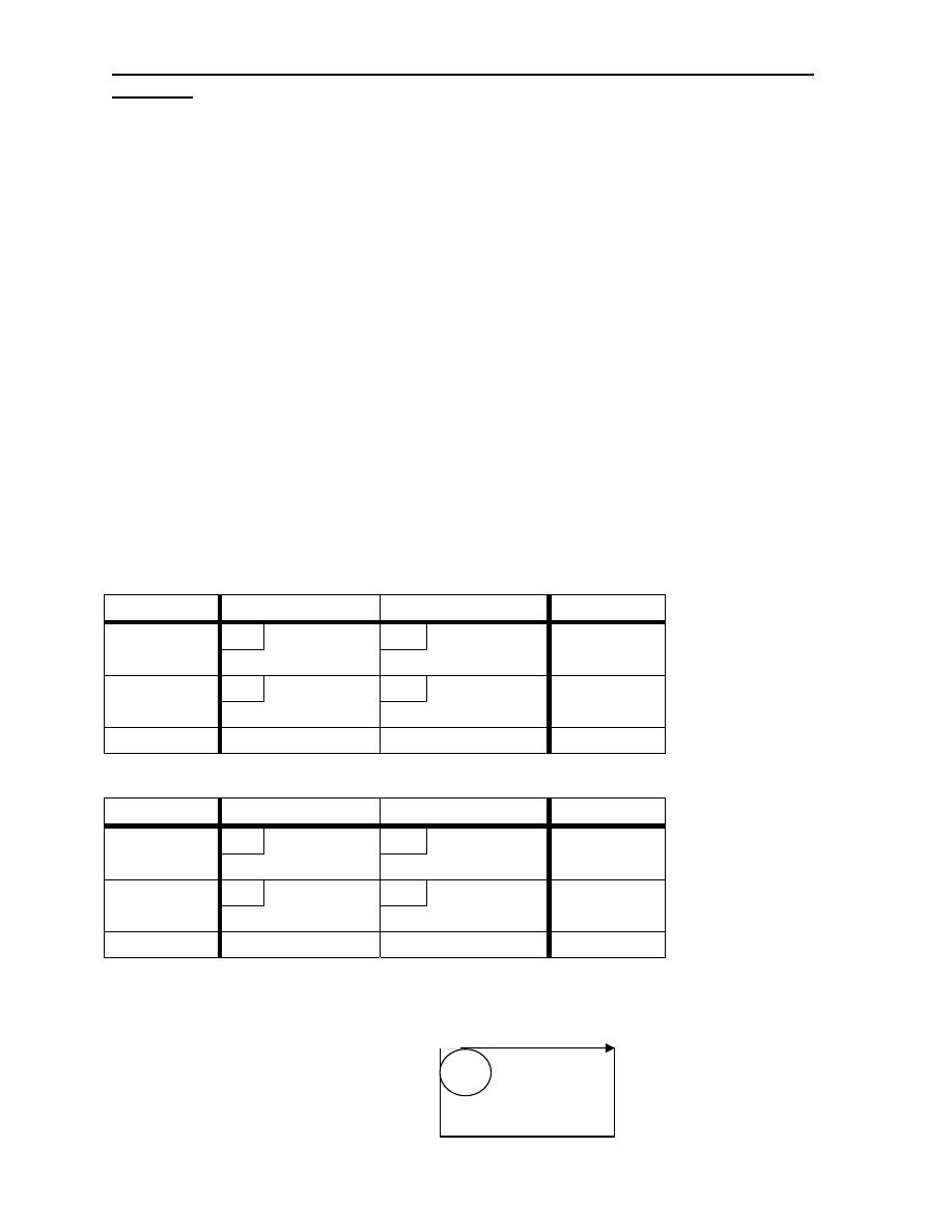
For example, suppose that three jobs must be assigned to three machines, each
machine must be assigned to only one job, and each job must be assigned to only
one machine.
The costs are shown below. Solve the problem by using the Hungarian algorithm.
Machines
Jobs
M1 M2 M3
A 25 31 35
B 15 20 24
C 22 19 17
Solution:
M1
M2
M3
M1
M2
M3
A 10 12 18
A 0 2 8
B 0 1 7
B 0 1 7
C 7 0 0
C 7 0 0
M1
M2
M3
M1
M2
M3
A 0 1 7
A 0 2 8
B 0 0 6
B 0
1 7
C 8 0 0
C 7 0 0
The assignment A-M
1
, B-M
2
20 , C-M
3
Min Z = 62
Maximization case:
Industrial Engineering (IE) - Dr. Khallel Ibrahim
Mahmoud
Use the Hungarian method to solve the same problem for the maximum
productivity.
Job
M1
M2
M3
A
25
31
35
B 15 20 24
C 22 19 0
M1
M2
M3
M1
M2
M3
A 10 4 0
A 0 0 0
B 20 15 11
B 10 11 11
C 13 16 18
C 3 12 18
M1
M2
M3
M1
M2
M3
A 0 0 0
A 1 0 0
B 0 1 1
B 0 0 0
C 0 9 15
C 0 8 14
C
ij:
No. of units produced per hour
Max C
ij
= 35
The final assignment :( two solution)
First Second
A M
3
A M
2
B M
2
20 B M
3
24
C M
1
C M
1
Unbalanced cases
If M≠N When M > N added dummy column with C
ij
= 0
Max or Min When M < N added dummy row with C
ij
= 0
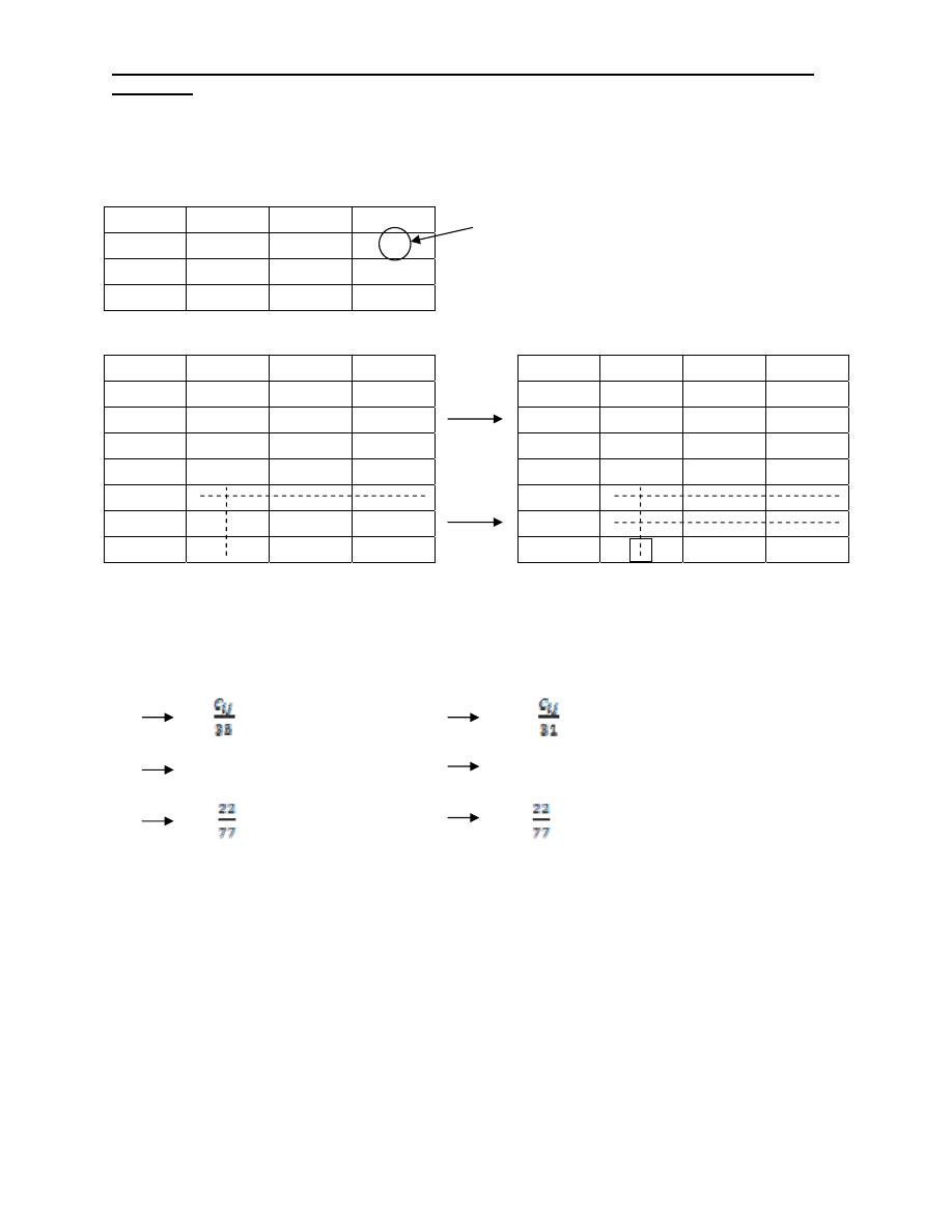
Example 1:
Industrial Engineering (IE) - Dr. Khallel Ibrahim
Mahmoud
Use the Hungarian algorithm to solve the assignment problem having the following
time table.
Solution:
Job M1 M2 M3 M4
J1 80 110 120
100
J2 50 160 130 80
J3 50 100 230
150
M1 M2 M3 M4
M1 M2 M3 M4
J1 80
110
120
100
J1 0 30 40
20
J2 50
160
130
80
J2 0 110
80
30
J3 50
100
230
150
J3 0 50
180
100
Dummy
J4
0 0 0
0
J4 0 0 0 0
M1 M2 M3 M4
M1 M2 M3 M4
J1 10 10 20 0
J1 0 10 20 0
J2 0 80
50
0
J2
0 90
60
10
J3 0 20
150
70
J3
0 30
160
80
J4
30
0
0
0
J4 20 0 0 0
M1 M2
M3
M4
J1 0 0 10
0
J2 0 70 40 0
J3 0 10 140
70
J4 40 0 0 10
The optimal assignment:
J1 – M2 110
J2 – M4 80
J3 – M1 50
J4 – M3 0
_________
240
Note: M<N
So we added dummy row with
C
ij
= 0
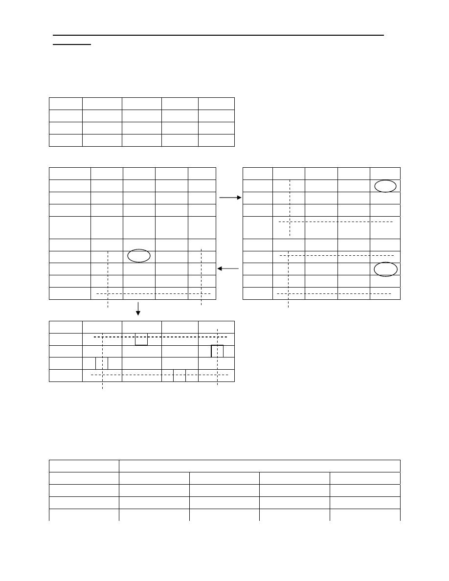
Example 2: Use the Hungarian algorithm to solve the following assignment
problem for the total maximum productivity.
Machines
Task M1 M2 M3 M4
T1 20 60 50 55
T2 60 30 80 75
T3 80 100 90 80
Industrial Engineering (IE) - Dr. Khallel Ibrahim
Mahmoud
T4 65 80 75 70
T5 70 65 60 65
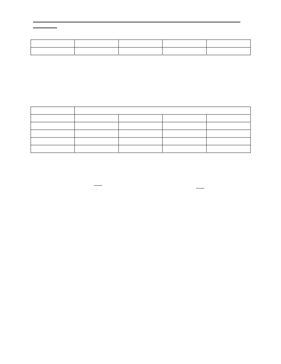
Example 3/ suppose four people can each perform any one of four different jobs
but possibly in different amount of time. The following table gives the
corresponding time to perform the various jobs. Which person should be assigned
to each job to minimize the total time to perform all four jobs?
Time to perform jobs
Person
1 2 3 4
A 2 10 9 7
B 15 4 14 8
C 13 14 16 11
D 4 15 13 9
Solution:
Ex 2: first solution, Cij
320
____
T5 – M1 70
T4 – M3 75
T3 – M2 100
Second solution, Cij
T1 – M5 0
T2 – M4 75
T1 – M5 0
T2 – M3 80
T3 – M2 100
T4 – M4 70
T5 – M1 70
____
320
Industrial Engineering (IE) - Dr. Khallel Ibrahim
Mahmoud
Industrial Engineering (IE)
Dr. Khallel Ibrahim Mahmoud
University of Technology
Electro-mechanical Engineering Dept.
Transportation Model
Lec.N
o(5)
2011
Industrial Engineering (IE) - Dr. Khallel Ibrahim
Mahmoud
Transportation Model
Introduction
The transportation model is a special class of the linear programming problem. It
deals with the solution in which an item is shipped from sources (e.g. factories) to
destinations (e.g. warehouses). The objective is to determine the amounts shipped
from each source to each destination that minimize the total shipping cost while
satisfying both the supply limits and the demand requirements.
The Mathematical Model
The general problem can be presented by the network.
-
There are M sources. S
1
,S
2
…………..S
m
-
And n destinations. D
1
,D
2
…………..D
n
-
The arcs linking the sources and destinations represent the routes between
the sources and the destinations.
-
The transportations cost per unit = C
ij
and the amount shipped = X
ij
-
The amount of supply at source i is ai and the amount of demand at
destination j is bj.
The objective of the model is to determine the unknown X
ij
that will minimize the
total transportation cost, while satisfying all the supply and demand restrictions.
a
1
a
2
a
i
Units of supply
a
m
S
1
S
2
S
i
S
Sources
D
D
D
j
x
m
x
13
c
m
c
13
c
12
x
12
x
11
D
c
11
Destination
b
1
b
2
b
j
b
n
Industrial Engineering (IE) - Dr. Khallel Ibrahim
Mahmoud
Objective Function:
Min Z:
C
ij
X
ij
Units of demand
Subject to:
j = 1,2,………………n
i = 1,2,………………m
1)
Determination of the starting
solution. The transportation model is always balanced (
=
) i.e. the
sum of supply= the sum of the demand. Thus, the model has Mth-1 basis
variables.
The special structure of the transportation problem allows securing a nonartificial
starting basic solution using one of three methods:
a-
North-west- corner method.
(N.W.C)
b-
Least-cost method. (L.C.M)
c-
Vogal method.
A)
N.W.C. method:
The method starts at the North West – corner cell of the tableau (variable X
11
).
Step 1: Allocate as much as possible to the select cell, and adjust the associated
amounts of supply and demand by subtracting the allocated amount.
Industrial Engineering (IE) - Dr. Khallel Ibrahim
Mahmoud
Step 2: Cross out the row or column with zero supply or demand to indicate that no
further assignments can be made in that row or column. If both the row and
column net to zero simultaneously, cross out one only, and leave a zero supply
(demand) in the uncrossed-out row (column).
Step3: If exactly one row or column is left uncrossed-out, stop. Otherwise, move to
the cell to the right if a column has just been crossed or the one below if a row has
been crossed out. Go to step1.
Example1:
In the following transportation problem use the north west- corner method
(N.W.C) to find the starting solution.
S/D D
1
D
2
D
3
Supply
S
1
5 3 10
150
S
2
3 9 8 70
S
3
11 10 7 80
S
4
6 13 6 40
Demand 160 120
60 340/340
Solution:
S/D D
1
D
2
D
3
ai
5 3 10
S
1
150
150
3 9 8
S
2
10
60
70
11 10
7
S
3
60
20
80
6 13 6
S
4
40
40
bj 160 120
60 340/340
Z= 5X150 + 3X10 + 9X60 + 10X60 +7X20 + 6X40
= 2300 M+N-1=6
B)
Least-Cost method:
Industrial Engineering (IE) - Dr. Khallel Ibrahim
Mahmoud
The Least-cost method finds a better starting solution by concentrating on the
cheapest routes. Instead of starting with the North West cell, we start by assigning
as much as possible to cell with the smallest unit cost (ties are broken arbitrary).
We then cross out the satisfied row or column, and adjust the amounts of supply
and demand accordingly. If both a row and a column are satisfied simultaneously,
only one is crossed out. Next, we always look for the uncrossed-out cell with the
smallest unit cost and repeat the process until we are left at the end with exactly
one uncrossed out row or column.
Example 2: the least -cost is applied to example (1)
S/D D
1
D
2
D
3
ai
5 3 10
S
1
30
120
150
3 9 8
S
2
70
70
11 10 7
S
3
20
60
80
6 13 6
S
4
40
40
bj 160 120
60 340/340
Z= 5X30 + 3X120 + 3X70 + 11X20 + 7X60 + 6X40
= 1600
C)
Vogal Method
Vogal method is an improved of version of the least cost method that generally
produces better starting solutions.
Step 1: For each row (each column) determine a penalty measure by subtracting
the smallest unit cost element in the row (column) from the next smallest unit cost
element in the same row (column).
Step 2: Identify the row or column with the largest penalty. Break ties arbitrarily.
Allocate as much as possible to the variable with the least unit cost in the selected
Industrial Engineering (IE) - Dr. Khallel Ibrahim
Mahmoud
row or column. Adjust the supply and demand and cross out the satisfied row or
column.
Step 3: a) If exactly one row or column with supply or demand remains uncrossed
out, stop.
b) If one row or column with positive supply (demand) remains uncrossed out,
determine the basic variables in the row (column) by the least-cost method, stop.
c) If all the uncrossed out rows and columns have (remaining) zero supply and
demand, determine the zero basic variables by the least-cost method.
d) Otherwise, go to step 1.
Example 3: Solve the transportation model of example (1) by using vogal method.
S/D D
1
D
2
D
3
ai V
1
V
2
V
3
V
4
V
5
V
6
5
3
10
S
1
30
120
150
2
5
3
9
8
S
2
70
70
5
5
5
11
10
7
S
3
20
60
80 3 4 4 4
4
6
13
6
S
4
40
40 0 0 0 0 0
bj 160 120
60 340/340
V
1
2
6
1
V
2
2 1
V
3
3 1
V
4
5
V
5
Z= 5X30 + 3X120 + 3X70 + 11X20 + 7X60 + 6X40
= 1600
Industrial Engineering (IE) - Dr. Khallel Ibrahim
Mahmoud
This solution happens to have the same objective value (1600) as in the Least-cost
method (L.C). usually, however vogal method is expected to produce better
starting solutions for the transportation method.
Stepping Stone Method (S.S)
After determining the starting ( using any of the three methods) we use one of the
following method :
1.
Stepping stone method.
2.
Modified distribution method.
So to solve a transportation problem, we first find an initial solution ( values of X
ij
)
and then improve the initial solution by reducing the cost through successive
iterations until the minimum cost solution is found.
Example:
S/D D
1
D
2
ai
6 3
S
1
70
8 7
S
2
100
bj 90 80
170/170
By using the N.W.C
S/D D
1
D
2
ai
6 3
S
1
70
70
8 7
S
2
20
80
100
bj 90 80
170/170
Z= 60X70 + 8X20 + 7X80
80
+
6 -
70
S
1
D
= 1140
Industrial Engineering (IE) - Dr. Khallel Ibrahim
Mahmoud
S/D D
1
D
2
ai
6 3
S
1
70
70
8 7
S
2
90
10
100
bj 90 80
170/170
Z= 1140 – 2X70 = 1000
3X70 + 8X90 + 7X10 = 1000
Unbalanced transportation problems
(
≠
)
Demand less than supply or demand greater than supply
(
<
) (
>
)
From/To A B
C
Dummy Factory
capacity
ai
5 4 3
0
D
250
250
8 4 3
0
E
50
200
50
300
9 7 5
0
F
150
150
300
Requirement
bj
300 200 200
150 700\850
-7
8
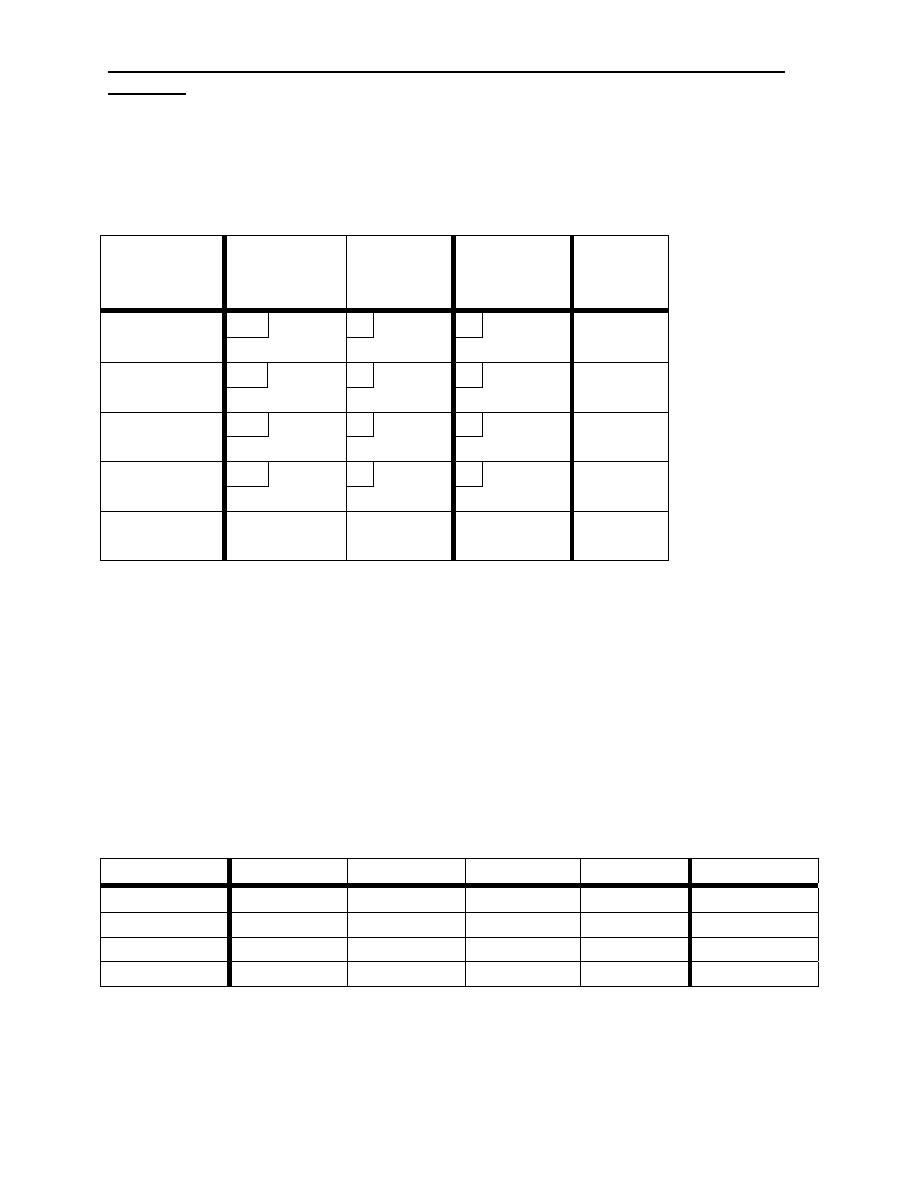
Industrial Engineering (IE) - Dr. Khallel Ibrahim
Mahmoud
Z = 3350
From/To A B C Plant
supply
ai
6 4 9
Plant W
200
200
10 5
8
Plant X
50
100
15
175
12
7
6
Plant Y
75
75
0 0 0
Dummy
plant
50
50
Requirement
bj
250 100 150
500\450
Z= 2850
Problems:
Q1/ Consider the following transportation problem. Find the starting solution by
using the following methods:
1-
N.W.C method.
2-
L.C method.
3-
Vogal method.
From/To C
1
C
2
C
3
C
4
Supply ai
V
1
2 2 2 1 3
V
2
10 8 5 4 7
V
3
7 6 6 8 5
Demand bj
4
3
4
4
15\15
Solutions:
1-
N.W.C = 93
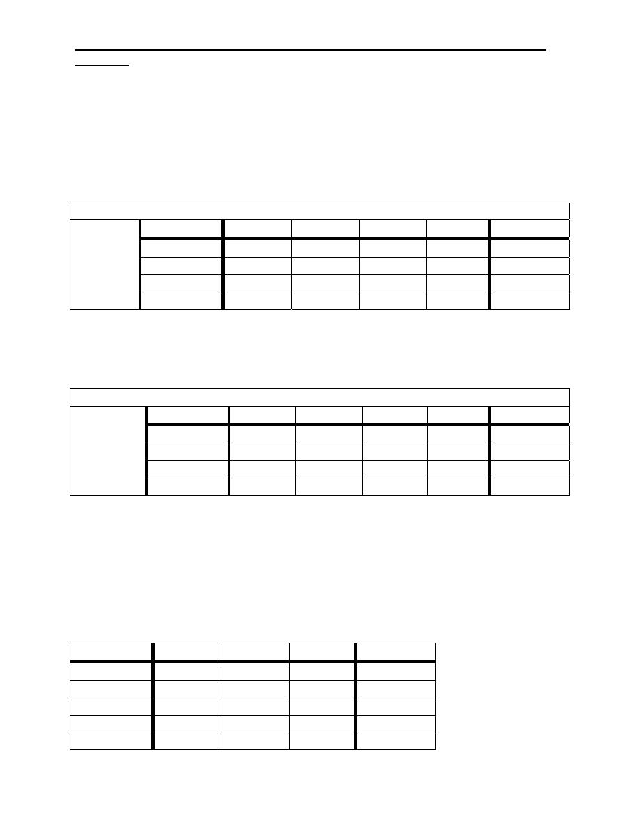
Industrial Engineering (IE) - Dr. Khallel Ibrahim
Mahmoud
2-
L.C = 79
3-
Vogal = 68
Q2 / Use the north west-corner method to find the starting solution (the initial
solution) for the following problem:
Warehouse
From/To D
1
D
2
D
3
D
4
Supply ai
S
1
0 4 0 2 5
S
2
1 2 5 6 10
S
3
5 3 7 9 15
Factory
Demand bj
20
10
15
15
60\30
Solution: Z= 65
Q3/ determine the initial solution for the following problem(use the three
methods).
Markets
From/To 1 2 3
4
Supply ai
A 10 8 6 4
2000
B 14
17 5 2
1300
C 18 7 11 9 1700
Warehouse
Demand bj
1000
2000
500
1500
5000\5000
Solutions:
1-
N.W.C Z= 52200
2-
L.C Z= 30700
3-
Vogal Z= 30700
Q4/ Use the northwest corner method to find the starting solution, then determine
the optimum solution by using (S.S) method for the following problem.
S/D D
1
D
2
D
3
ai
S
1
5 3 10 150
S
2
3 9 8 70
S
3
11 10 7 80
S
4
6 13 6 40
bj 160
120
60
340\340
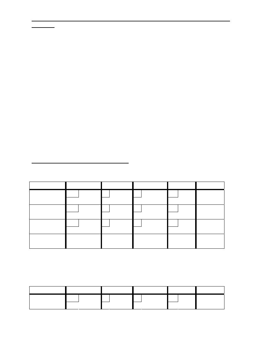
Industrial Engineering (IE) - Dr. Khallel Ibrahim
Mahmoud
Z
0
= 2300
Z
1
= 2300 – 8X60 = 1820
Z
2
= 1820 – 5X40 = 1620
Z
3
= 1620 – 1X20 = 1600
Solutions for transportation method:
Q1/ N.W.C method
From\To C1 C2 C3 C4 ai
2 2 2
1
V1
3
3
10 8
5
4
V2
1
3
3
7
7
6
6
8
V3
1
4
5
bj 4 3 4
4
15\15
4+3-1 = 6
Z= 2X3 + 1X10 + ……. +8X4 = 93
L.C.method
From\To C1 C2 C3 C4 ai
2 2 2
1
V1
3
3
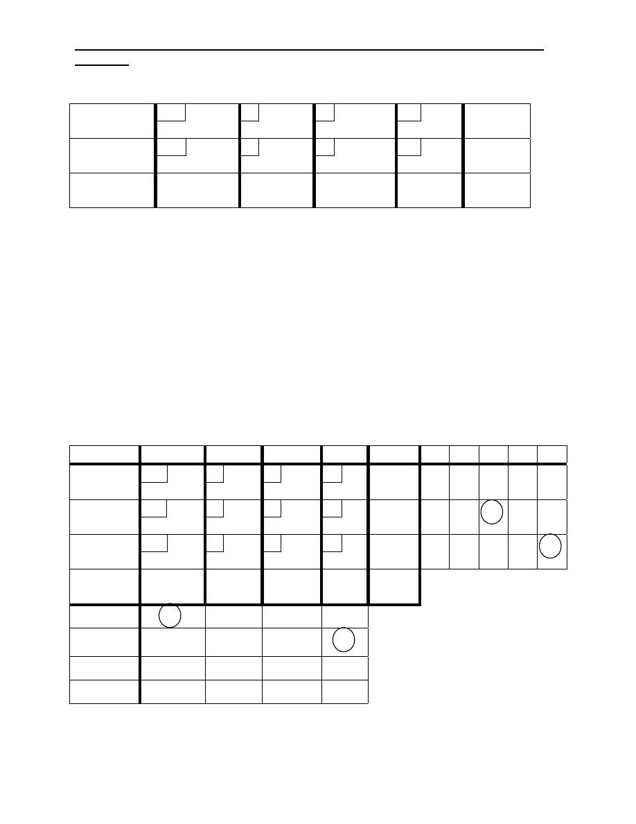
Industrial Engineering (IE) - Dr. Khallel Ibrahim
Mahmoud
10 8
5
4
V2
2
4
1
7
7
6
6
8
V3
2
3
5
bj 4 3 4
4
15\15
4+3-1 =6
Z = 1X3 + 1X4 + …… + 6X3 = 79
Vogal method
From\To
C1
C2
C3
C4
ai U1 U2 U3 U4 U5
2 2 2
1
V1
3
3 1
10 8
5
4
V2
3
4
7 1
1
3
7
6
6
8
V3
1
3
1
5 0 0 0 0 1
bj 4 3 4
4
15\15
U1 5 4 3
3
U2 3 2 1
4
U3 3 2 1
U4
Z = 2X3 + 5X3 +…… + 6X1 = 68
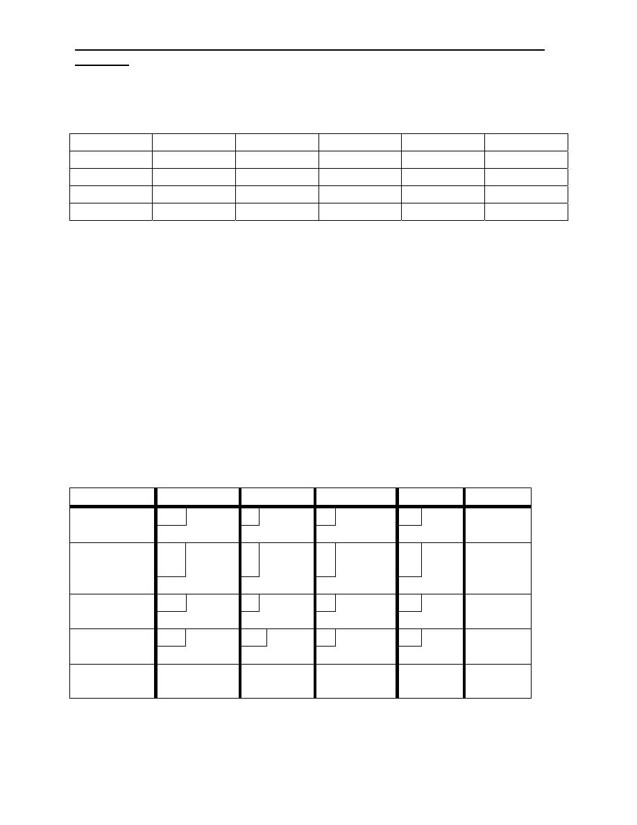
Industrial Engineering (IE) - Dr. Khallel Ibrahim
Mahmoud
Q2: ∑ ai ≠ ∑ bj
From
\To
D1 D2 D3 D4 ai
S1 0 4 0 2 5
S2 1 2 5 6 10
S3 5 3 7 9 15
bj 20 10 15 15
60\30
N.W.C method ∑ bj - ∑ ai = 30
From\To D1 D2 D3 D4 ai
0 4 0
2
S1
5
5
1 2
5
6
S2
10
10
5
3
7
9
S3
5
10
15
0 0
0
0
Dummy S4
0
15
15
30
bj 20 10
15
15
60\60
Z = 0X5 + 1X10 +…….. + 0X15 = 56
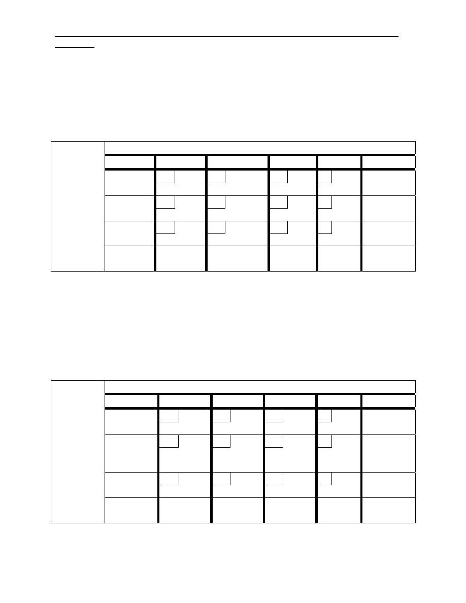
Industrial Engineering (IE) - Dr. Khallel Ibrahim
Mahmoud
Q3:
L.C.M
Market
From\To 1
2
2 4
ai
10 8
6 4
A
1000
300
500
200
2000
14 17
5
2
B
1300
1300
18
7
11
9
C
1700
1700
warehouse
bj 1000 2000 500
1500
5000\5000
Z= 10X1000 + ……. + 7X1700 = 30700
N.W.C
Market
From\To 1
2
2 4 ai
10 8 6 4
A
1000
1000
2000
14 17
5
2
B
1000
300
1300
18
7
11
9
C
200
1500
1700
warehouse
bj 1000
2000 500
1500
5000\5000
Z = 10X1000 + …………….. + 9X1500 = 52200
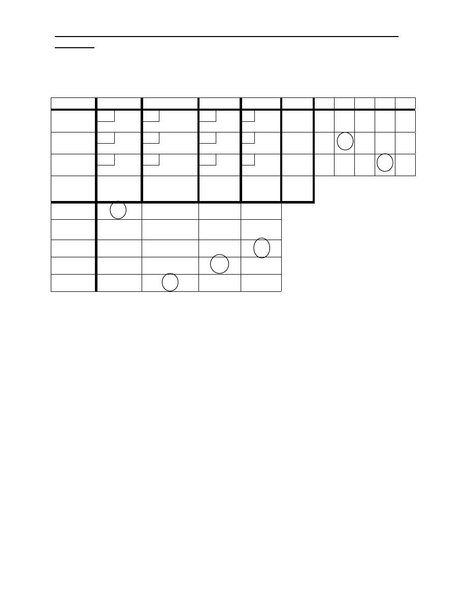
Industrial Engineering (IE) - Dr. Khallel Ibrahim
Mahmoud
Vogal method
From\To
1
2
3
4
ai V1 V2 V3 V4 V5
10 8
6 4
A
1000
300
500
200
2000 2 2 2 2
14 17
5
2
B
1300
1300
3 3
18
7
11
9
C
1700
1700 2 2 2 4
bj 4 3 4 4
15\15
V1 4 1 1 2
V2 1 1
V3 1 5 5
V4 1 5
V5 1
Z = 10X100 + ………. + 7X1700 = 30700