Lecture 8 - Sampling distribution
80
It is the distribution of all possible values of statistics
computed from samples of the same size randomly drawn
from the same population.
When sampling is from normally distributed population,
the distributions of the sample will possess the following
properties:
1) The distribution of the sample means(x) will be normal.
2) The mean of the distribution of the x will be equal to the
mean of population (µ).
3) The variance of the distribution of X will be equal to the
variance of the population divided by the size of the
sample ∂
2
/n = ∂/√n.
As the sample size increase, the following of distribution
of sample mean to normal distribution will be increase.
Sampling error: is the difference between the value of a
sample statistic and the value of the corresponding
population parameter. In the case of the mean,
EX: In a recent exam, assume that the distribution of
scores of all examinees is normal with the mean of 1020
and a standard deviation of 153. Calculate the mean and
standard deviation of and describe the shape of its
sampling distribution when the sample size is 16, 50,
1000
Steps in constructing sampling distribution:
1) Form a population of size (N) and randomly draw all
possible samples of size (n). EX: If there is a population
of 5 individuals & we want to take a sample of size 2,
then we can draw 10 samples, and so 10 probabilities for
a sample of size 2.
2) For each sample we compute the statistic of interest
(sample mean).
3) Make a table for the observed value of the statistic and its
corresponding frequencies. So for every value of a
statistic we have certain frequency and we take the mean
of every sample with its corresponding frequency and by
plotting on the X and Y axes, we will get a normal
distribution curve. So the change is from X to μ
x
curve
and we can convert it into z table and find the
corresponding probability as.
The distribution of μx will be normal.
The mean of the distribution of the values of μ
x
will be
the same as the mean of the population from which the
samples were drawn. (i.e. if we get all the possible
samples and take the mean of each one and them take
the mean of these means; we will get the underlying
population mean).
The variance of the distribution of μ
x
, will be equal to
the variance of the population divided by the sample
size; = δ
2
/n, which is the variance of the underlying
population divided by the sample size. (standard error)
δ
2
x = variance / sample size = δ
2
/n or δ/√n
Z-value for Sampling Distribution of the Mean
(Distribution of the sample mean):
When sampling is from a normally distributed population
then the mean of the sample will follow the normal
distribution, while if sampling is from a non-normally
distributed population it will follow the central limit
theory; with increasing sample size sampling will
approximate the normality or its curve will be similar to
that of NDC, e.g. a sample of 1000 person will follow the
normal distribution more than a sample of 5 persons.
Z = (x - µ) / (∂/√n)
** It is important to know that we use Z-distribution when
the variance (or standard deviation) of the population is
known or the sample size more than 60.
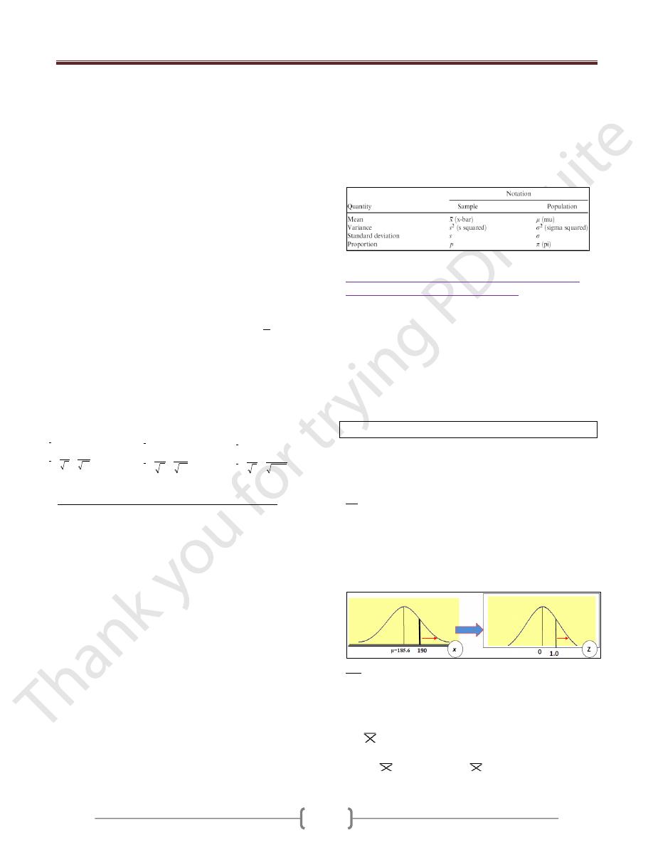
Ex If the cranial length of certain large human population
which is normally distributed µ= 185.5 mm and ∂ = 12.7
mm, what is the probability of a random sample of size
n=10 from this population will have x ≥ 190mm?
Z = (x - µ) / (∂/√n)
= (190-185)/ (12.7/√10) = 1.09.
P(x ≥ 190) → P ( Z ≥ 1.09). & From the Z-table, P=0.1379.
Ex: If the mean and standard deviation of serum iron
values for health men are 120 and 15 μg per 100 ml,
respectively, what is the probability that a random sample
of 50 normal men will yield a mean between 115 and 125
per 100 ml?
Z =
- μ / (δ/√n) = (115-120)/(15/√50) = -2.36
(125-120)/(15/√50) = 2.36
P (115≤
≤ 125) = P(-2.36≤
≤ 2.36) = 0.9909-0.0091=
0.9818
250
.
38
16
153
1020
n
x
x
637
.
21
50
153
1020
n
x
x
838
.
4
1000
153
1020
n
x
x
x
Lecture 8 - Sampling distribution
81
Distribution of the difference between two sample
means
Giving 2 normally distributed population with means of
µ
1
& µ
2
and variances of ∂
1
& ∂
2
, the random samples
drawn from these population with size n
1
& n
2
are
normally distributed and the difference between the
means (x
1
-x
2
) will be also normally distributed, with mean
equal to (µ
1
- µ
2
) and variance equal to (∂
1
2
/ n
1
)+ (∂
2
2
/ n
2
).
Or Tow normally distributed population with means of
(μ
1
) & (μ
2
) and variances of (δ
2
1
) & (δ
2
2
) respectively. The
sampling distribution of the difference of
1
ــ
2
between the means of independent samples of size n
1
& n
2
drawn from these populations is normally distributed with
mean μ
1
-μ
2
and variance of [√(δ
2
1
/n
1
) + ( δ
2
2
/n
2
)].
Z =(x
1
-x
2
) - (µ
1
- µ
2
) / √ (∂
1
2
/ n
1
)+ (∂
2
2
/ n
2
).
Ex. If the level of vit.A in the liver of 2 human population
normally distributed ∂
1
2
= 1900, ∂
2
2
= 8100. What is the
probability that random sample of size n
1
= 15 & n
2
= 10
will give a value of (x
1
-x
2
) ≥50? Suppose there is no
difference in population means.
Z =(x
1
-x
2
) - (µ
1
- µ
2
) / √ (∂
1
2
/ n
1
)+ (∂
2
2
/ n
2
).
= 50- 0 / √ 1900/15 + 8100/10 = 1.09
P(x
1
-x
2
≥ 50) → P (Z ≥ 1.09). & From the Z-table,
P=0.1379.
Ex: For population of 17 year-old, the means & standard
deviations of subscapular skinfold thickness values (in
mm) for boys 9.7 & 6 & for girls 15.6 & 9.6 respectively.
Simple random samples of 40 boys & 35 girls are
selected, what is the probability that the difference
between sample means will be greater than 10? 0.0139
Distribution of the sample proportion
Proportion = part/whole (the numerator is part form the
denominator).
When the sample size is large ((≥30)), the distribution of
sample proportion (P) is approximately normally
distributed. The mean of the distribution will be equal to
the true population proportion, and the variance of the
distribution will be equal to P (1-P)/n. We can use Z-
distribution, and to calculate Z:
Z= [
p
ˆ
-P] / [√P (1-P)/n]
Or The
distribution is binomial, but for larger samples (≥
30) the distribution will be approximately normally
distributed and have the following characteristics:
μ
p
= P, δ
2
p
= {P(1-P)}/n & δ
p
= √[{P(1-P)}/n ],
so Z= [
p
ˆ
-P] / [√P (1-P)/n]
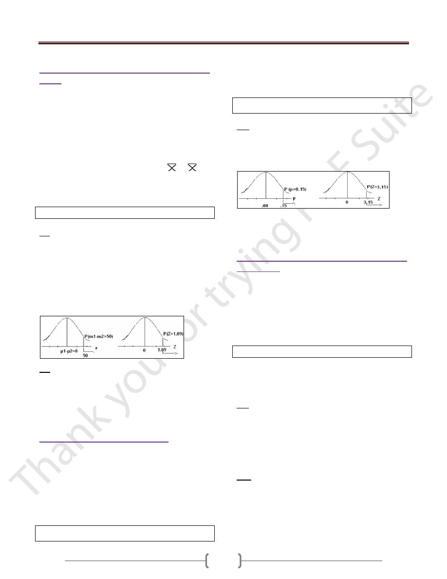
Ex: suppose in a certain human population the proportion
of color blindness is 8%, if randomly we select 150
individuals from this population, what is the probability
that the proportion of color blindness in this sample will
be greater than 15%?
Z= [
p
ˆ
-P] / [√P (1-P)/n]
= [0.15-0.08] / [√o.o8 (1- 0.08) /150] = 3.15
P(P ≥ 15%) → P (Z ≥ 3.15). & From the Z-table, P=0.0008
Distribution of the difference between two sample
proportions:
If independent random samples of size n
1
& n
2
are drawn
from two populations where the proportions of
observation in the two populations are P
1
& P
2
, the
distribution of the difference between samples proportions
(P
1
- P
2
) is approximately normally and the variance of the
distribution will be equal to[ P
1
(1-P
1
)/n
1
]+ [P
2
(1-P
2
)/n
2
] .
We can use Z-distribution, and to calculate Z:
Z= (P
1
-P
2
) - (P
1
-P
2
) / √[P
1
(1-P
1
)/n
1
]+ [P
2
(1-P
2
)/n
2
]
Characterized by: μP
1
-P
2
= P
1
-P
2
δ
2
P
1
-P
2
={P
1
(1-P
1
)}/n
1
+ {P
2
(1-P
2
)}/n
2
→ δP
1
-P
2
=
√[{P
1
(1-P
1
)}/n
1
+ {P
2
(1-P
2
)}/n
2
], so
Z = [(P
1
-P
2
)-(P
1
-P
2
)] / √[{P
1
(1-P
1
)}/n
1
+ {P
2
(1-P
2
)}/n
2
]
Ex: In a certain population of teenagers the proportion of
obese boys (P
1
= 10%), and the proportion of obese girls
(P
2
= 10%), what is the probability that a random sample
of boys n
1
=250 and girls n
2
= 200 will yield P
1
-P
2
≥ 0.06?
Z= (P
1
-P
2
) - (P
1
-P
2
) / √ [P
1
(1-P
1
)/n
1
] + [P
2
(1-P
2
)/n
2
]
= (0.06)-(0.1-0.1) / √ [0.1(1-0.1)/250] + [0.1(1-0.1)/200] = 2.11
P (P
1
-P
2
) ≥ 0.06→ P (Z ≥ 2.11). & From the Z-table, P=0.017
Ex: A random sample of medical students from third &
fifth years was chosen to study the extent of self-
medication practices among them. Out of 110 students in
the 3
rd
year, 38% reported self-medication compared to 60
out of 95 of fifth year students. Apply a suitable statistical
test to confirm apparent difference in self medication
practices between the 2 groups of medical students
.
_ _
~