20
Lecture 3 - Transform and Recode Data
SPSS allows one to recode or transform existing data into different forms.
Recode Data
Recoding data assigns new values to existing data, or collapses subsets of data into new
values. For example, we might want to group our six students by whether they scored
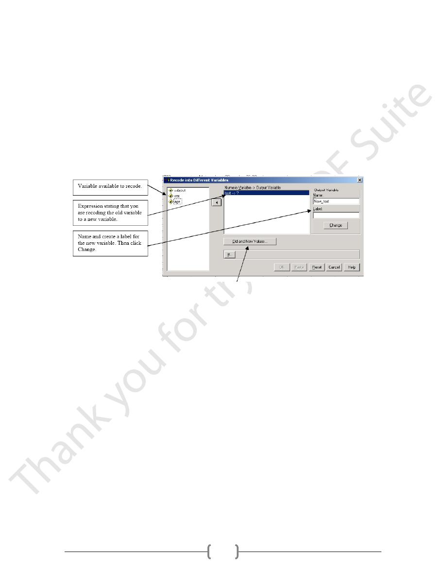
high or low on the test. To do this, select Transform → Recode. At this point you have
the option of recoding to the same or different variables. To recode to the same variable
would replace the existing data with the new codes. To recode to a different variable
would create a new variable with the new codes.
The second is almost always my preference because it allows you to retain your original
data.
We selected test to recode into a new variable called New_test. To identify the new
values, click
Old and New Values.
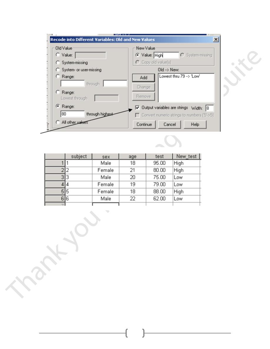
You must identified the old value or range of values and the new, recoded value. You can
either recode individual values or a range of values.
In this case, all test scores less than 80 were considered low and all that were 80 or higher
were considered high. For the low range, select Range, Lowest Through 79 for Old
Value. For new value, if the output is a string variable as it is here, check, “Output
variables are strings,” and enter the new value to match the old range (Low). Then click
Add.
For the high range, the parameters are listed in the window above. Then click Add. Click
Continue when done.
21
SPSS creates a new variable with the recoded values:
Transform Data
You can compute new variables as a function of old variables. For example, a new
variable could be the sum of two old variables. The new variable could be the square root
of an old variable.
There are almost infinite possibilities for transforming data. To transform data, select
Transform → Compute.
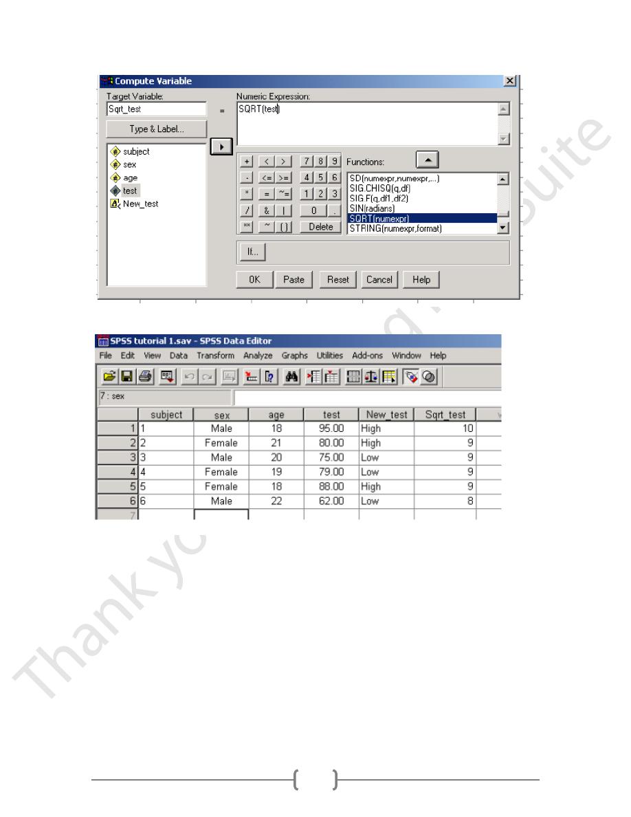
Use the expression builder to design your new variable:
In Target Variable, type the name of the new variable that will contain the transformed
values. The Numeric Expression box identifies how to compute the transformed values.
Use this box similarly to that used in Selecting Cases. Here we have created a new
variable that is equal to the square root of test.
22
SPSS will create a new variable with values equal to the square root of test for each case.
Descriptive Statistics
Descriptive statistics convert large sets of data to more meaningful, easier to interpret,
chunks or values. They summarize the data. Examples include the mean, median,
variance, and range.
SPSS contains a function that will compute many of these statistics, easily.
Simply select Analyze → Descriptive Statistics → Descriptives.
23
A new window will appear with two boxes. As before, the box on the left contains
variables with which descriptive statistics may be calculated (i.e., numeric variables).
Move the variables of interest to the right-hand box with the arrow button.
By default, SPSS will provide the following: (a) mean, (b) standard deviation, (c) sample
size (d) minimum value, and (e) maximum value.
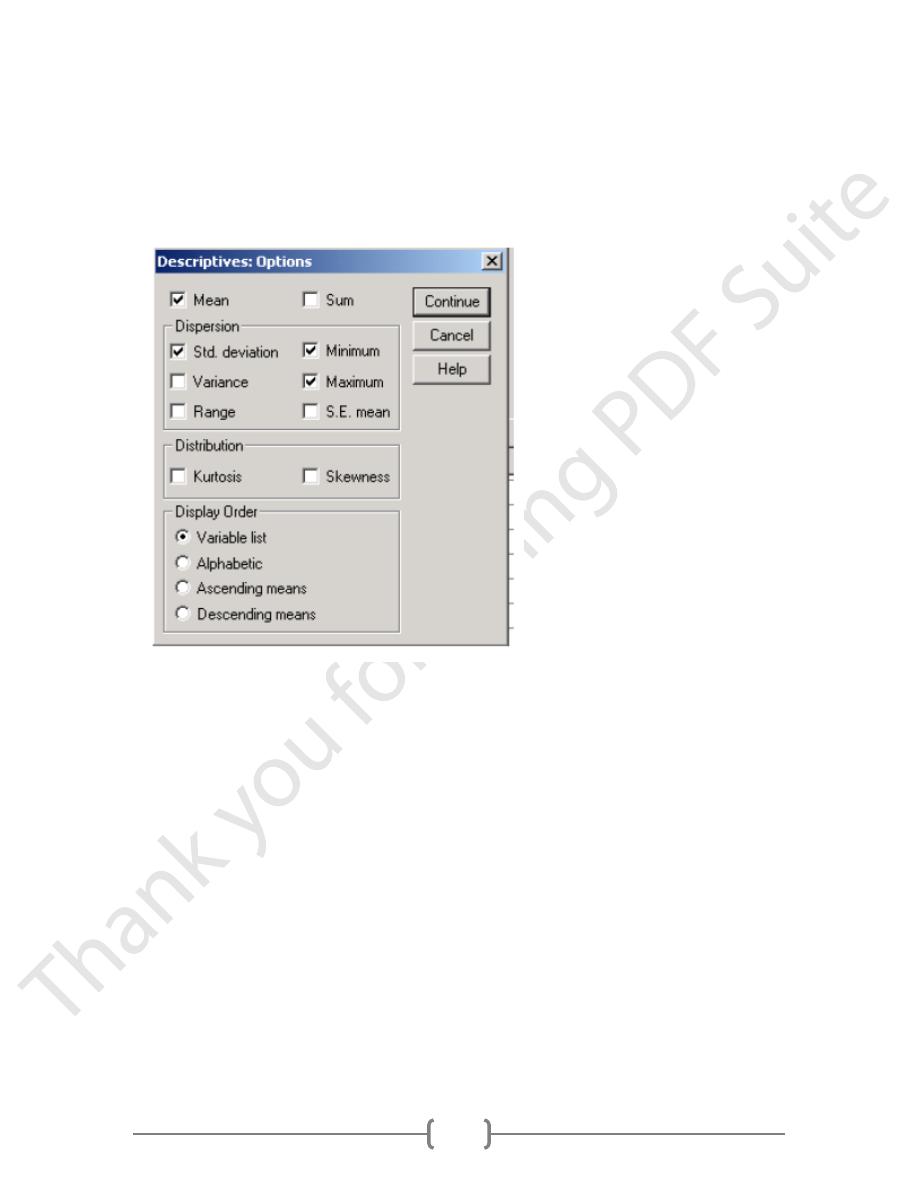
To select additional options or de-select default options, click the Options button.
Any item with a check-mark will be computed, for each variable selected in the previous
step.
Under display order, you may select the order in which the variables appear in the output.
When you are finished, click Continue to return to the variable-selection window and
click OK.
SPSS will compute the statistics and open a new window (Output) with the descriptive
statistics.
Reading SPSS Output
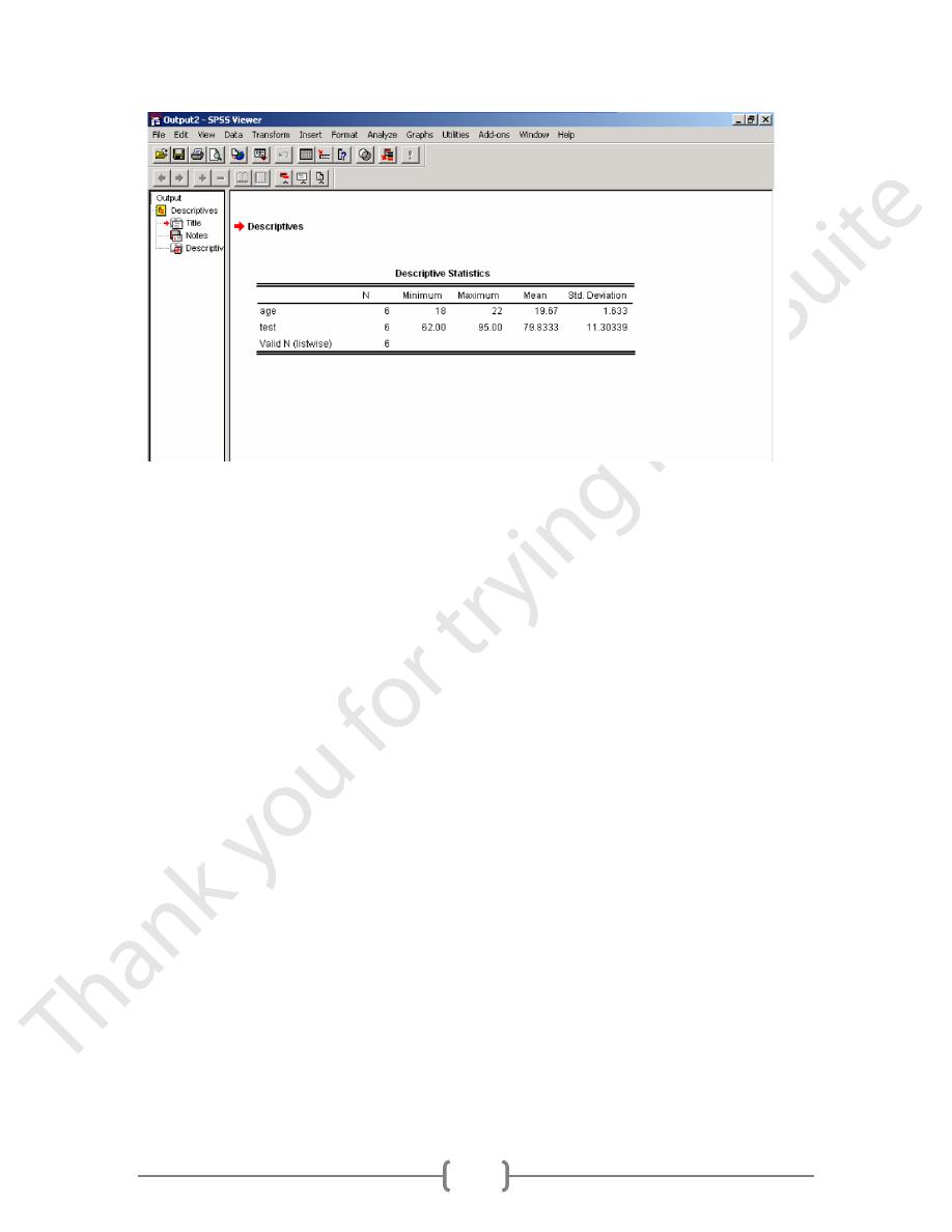
The following output is the result of selecting the variables age and time.
24
Notice there are two frames: the one on the left lists all the analyses available for
viewing, as well as any notes and titles relating to those analyses; the one on the right
depicts the results of the analyses.
Typically, SPSS reports results in tabular form. The variables are listed on the left
followed by the statistics we selected earlier. We can see that the average age is 19.67
with a standard deviation of 1.633.
SPSS will report variable names or labels or both. To change the default setting, go to
Edit →Options → Output labels.
How to split groups
If you want to calculate descriptive statistics on sub-groups (such as males and females
separately), you may split your files. To do this:
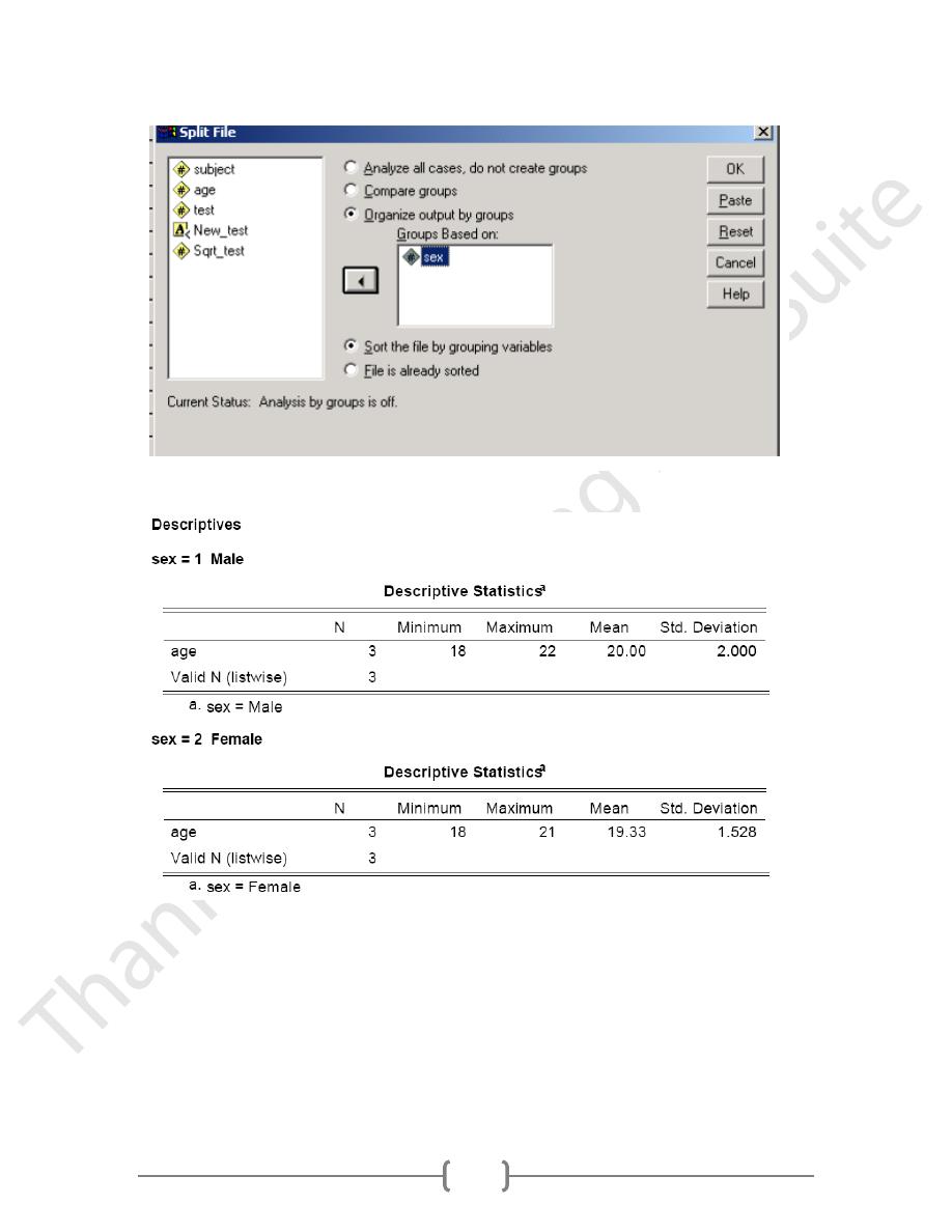
Data → Split File
Determine how you want to split your data set.
To separate by sex, select Organize output by groups and move the variable sex to the
right-hand window. Then select OK.
25
When you run descriptive statistics on any variable, they will be reported for each level
of sex. See below:
26
Frequency Tables
Frequency tables include lists of values (categories) within each selected variables and
the number of times each category occurs.
To create a table of frequencies (number of occurrences of given categories), select
Analyze →Descriptive Statistics → Frequencies.
Select the variables to be depicted in the frequency table by moving them from the left- to
the right-hand box. SPSS provides the user additional options, including statistics, charts,
and
format.
Statistics
SPSS will, by default, print the values of the selected variables and the frequencies of
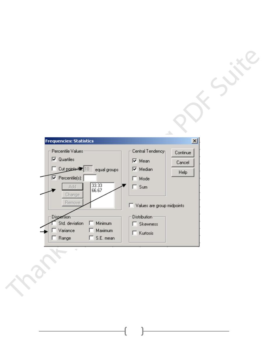
each. If you prefer additional information, click Statistics:
Options include percentile values. SPSS will print quartiles (fourths) or the values that
divide the data into X equal groups (cut points). The number of groups is defined by
the user. SPSS will also print selected percentiles. Simply, select Percentile(s), then
type in the percentile of interest and click Add. We have selected thirds.
You may also select descriptive statistics, like measures of central tendency and
dispersion, as well as statistics describing the distributions.
When finished, select Continue.
Charts
27
This option allows users the opportunity to view bar charts, pie charts, or histograms in
addition to the frequency table. This might be useful if there are many categories for each
variable or if two or more variables are to be compared. The charts may contain
frequencies or percentages.
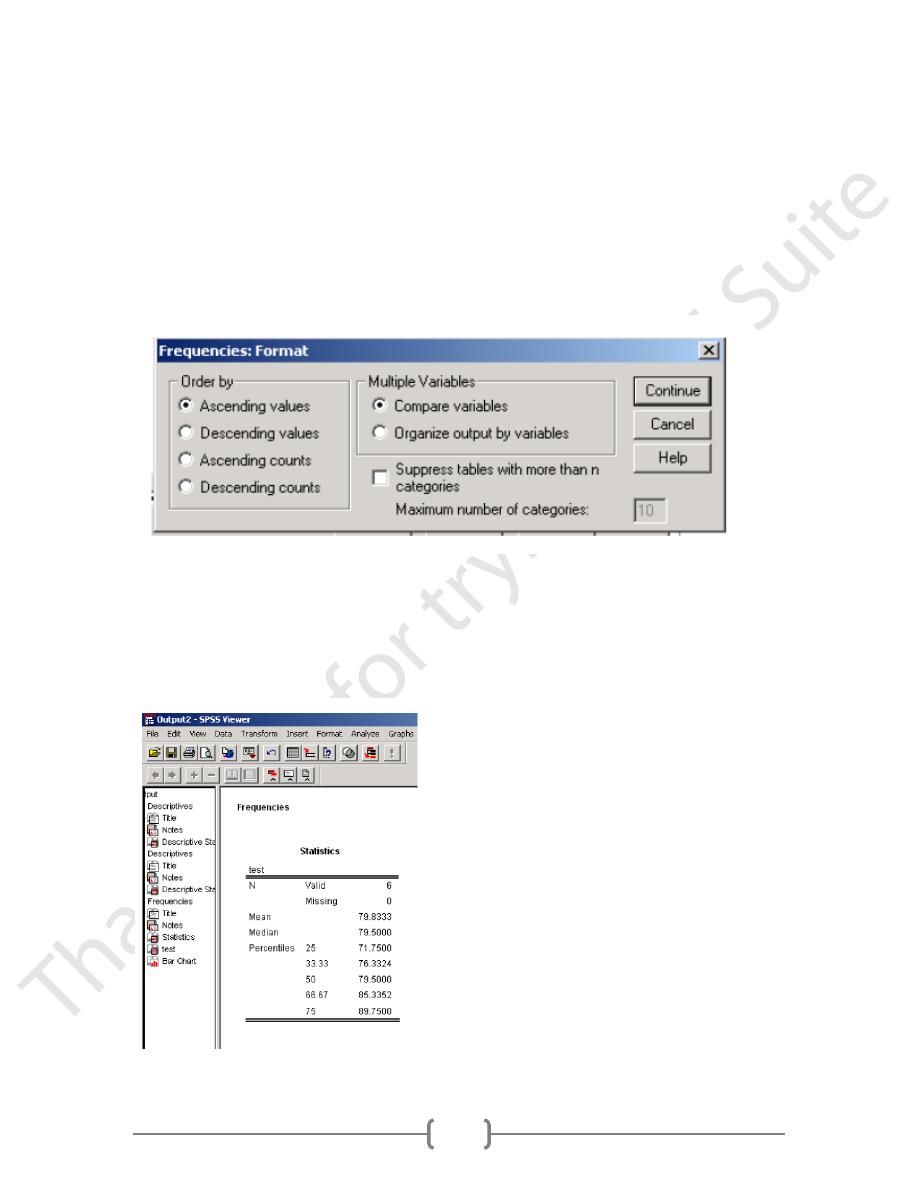
Format
With this option, users can determine the order in which categories will appear and
whether or not multiple variables should be compared. This will impact how results are
presented.
To cut back on the amount of output ,users may choose not to view tables with many
categories (categories).
When finished click Continue to return to the variable-selection window. Then click OK.
The new analyses are added to the descriptive statistics. Notice the addition in the left-
hand frame.
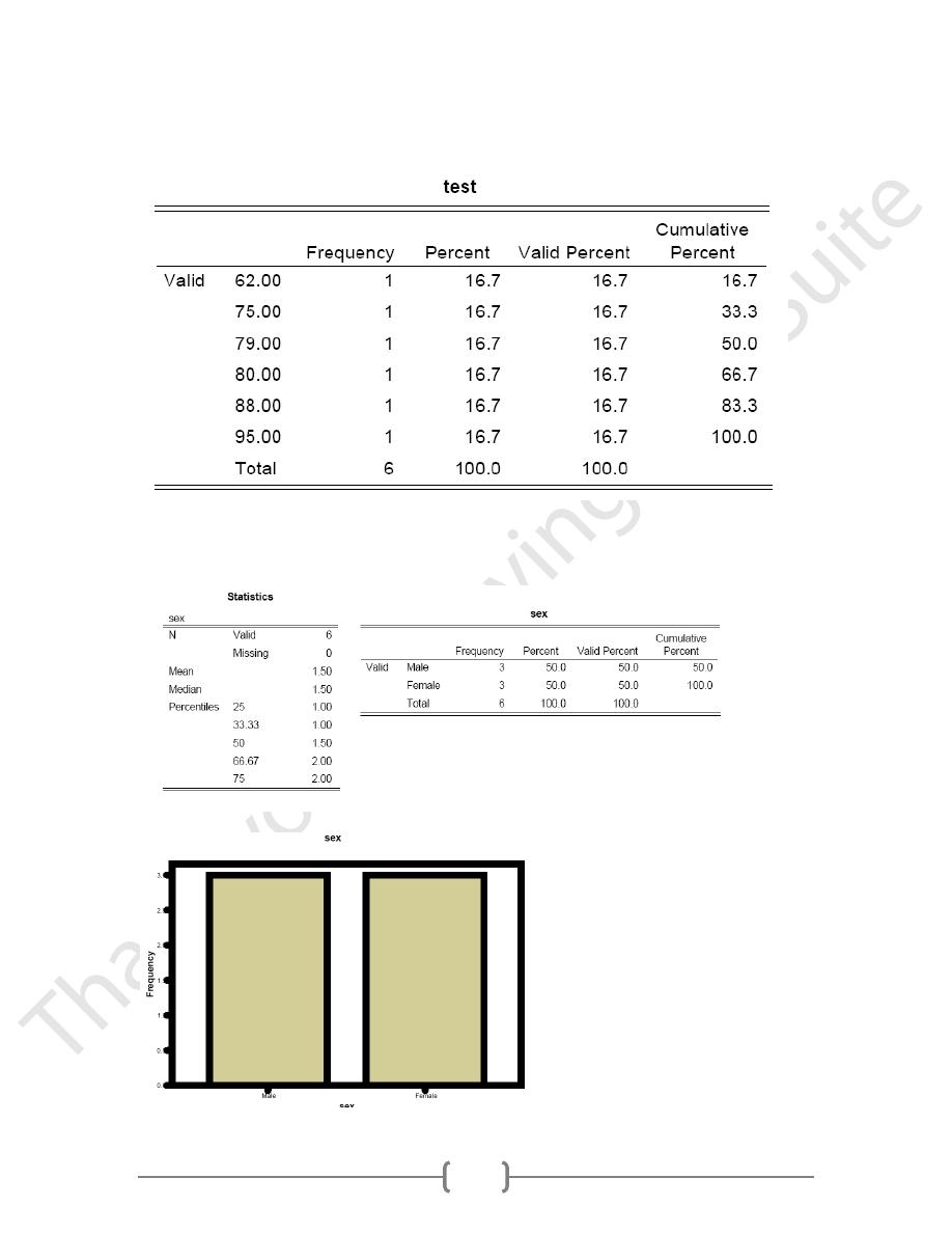
The following statistics are for the variable test.
Notice there are a total of six cases, and none
are missing. The mean test score is 79.833, the
median is 79.5. The value of 71.75 cuts off the
25
th
percentile (25% of cases fall at or below
this value), and so on.
28
If we scroll down the page, we will find additional results:
This table lists all the values of the variable test and the frequency of occurrence of each.
Notice there is only one occurrence of each value.
Next, SPSS provides a bar chart depicting these frequency results, as selected under
Charts. However, it is not of great interest because the frequency is 1 for each value.