97
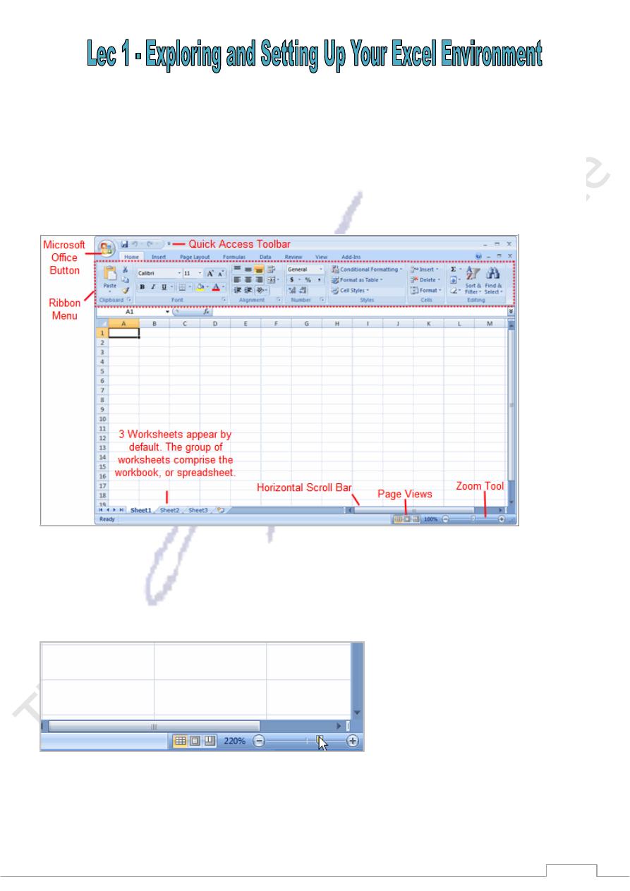
The tabbed Ribbon menu system is how you navigate through Excel and access the various Excel
commands. If you have used previous versions of Excel, the Ribbon system replaces the traditional menus.
Above the Ribbon in the upper-left corner is the Microsoft Office Button. From here, you can access
important options such as New, Save, Save As, and Print. By default the Quick Access Toolbar is pinned
next to the Microsoft Office Button, and includes commands such as Undo and Redo.
At the bottom, left area of the spreadsheet, you will find worksheet tabs. By default, three worksheet tabs
appear each time you create a new workbook. On the bottom, right area of the spreadsheet you will find
page view commands, the zoom tool, and the horizontal scrolling bar.
To Zoom In and Out:
Locate the zoom bar in the bottom, right corner.
Left-click the slider and drag it to the left to zoom out and to the right to zoom in.
To Scroll Horizontally in a Worksheet:
Locate the horizontal scroll bar in the bottom, right corner.
Left-click the bar and move it from left to right.
98
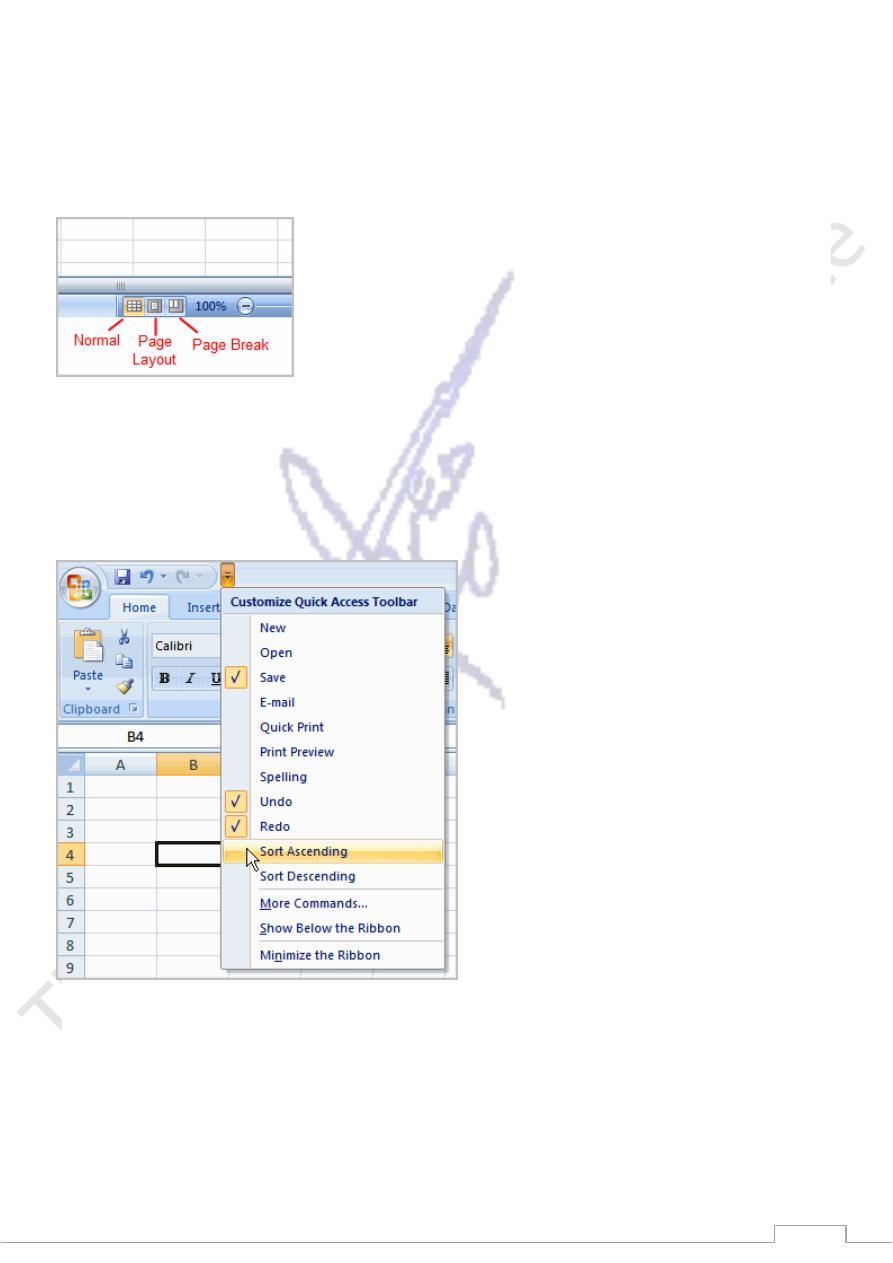
To Change Page Views:
Locate the Page View options in the bottom, right corner. The Page View options are Normal, Page
Layout, and Page Break.
Left-click an option to select it.
The default is Normal View.
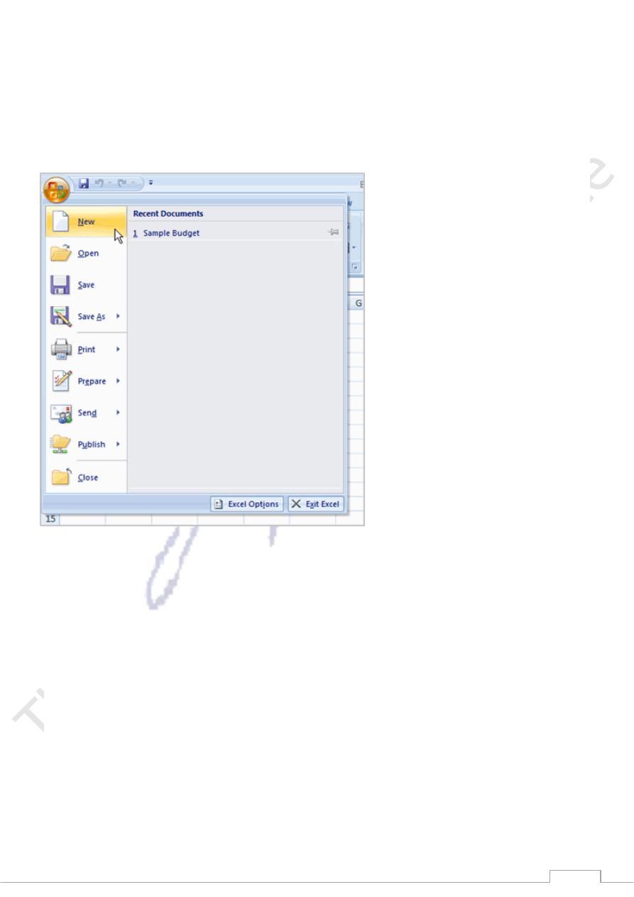
To Add Commands to the Quick Access Toolbar:
Click the arrow to the right of the Quick Access toolbar.
Select the command you wish to add from the drop-down list. It will appear in the Quick Access
toolbar.
OR
Select More Commands from the menu and a dialog box appears.
Select the command you wish to add.
Click the Add button.
Click OK.
The Save, Undo, and Redo commands appear by default in the Quick Access toolbar. You may wish to add
other commands to make using specific Excel features more convenient for you
99
Your First Workbook
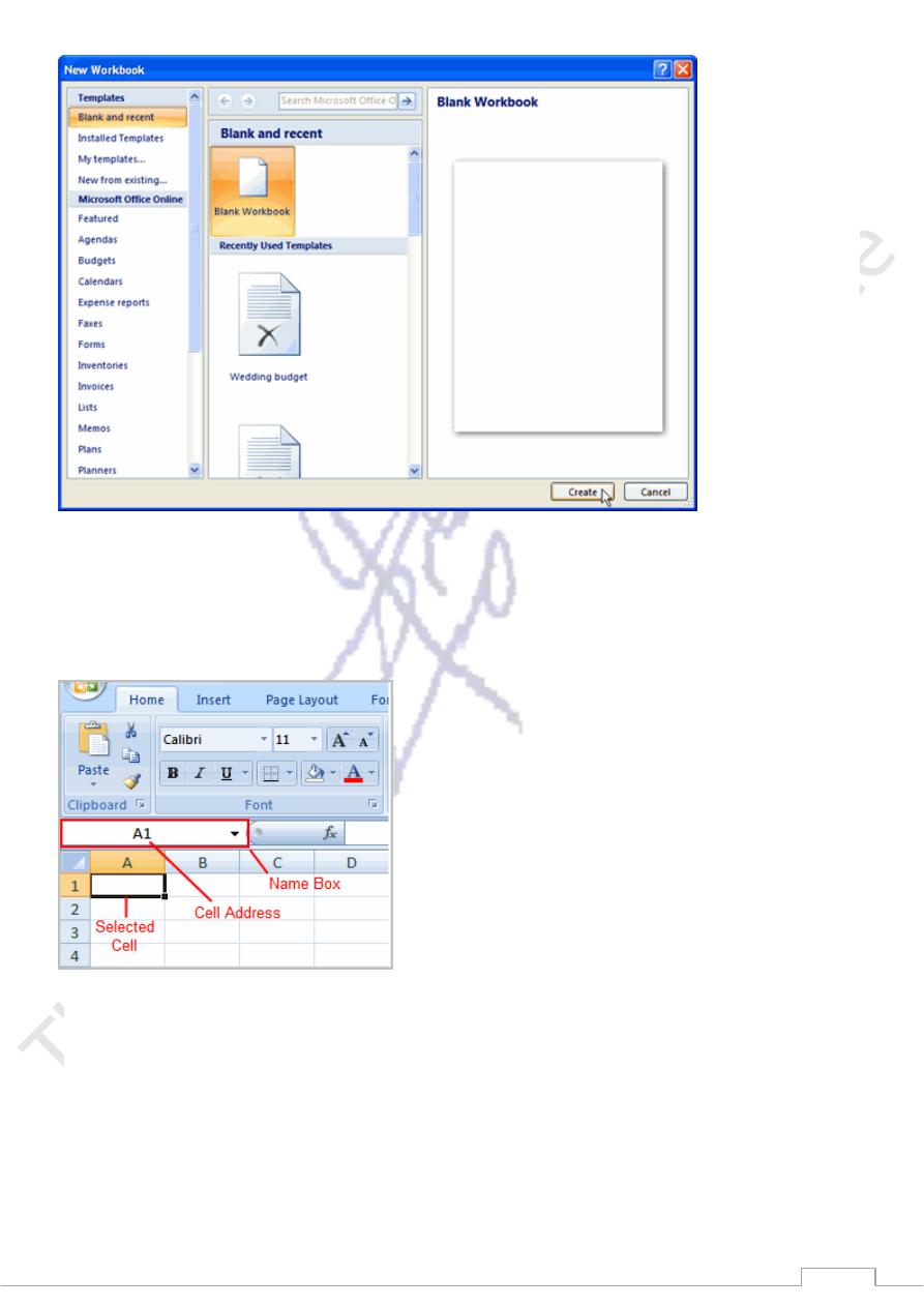
To Create a New, Blank Workbook:
Left-click the Microsoft Office Button.
Select New. The New Workbook dialog box opens and Blank Workbook is highlighted by default.
Click Create. A new, blank workbook appears in the window.
111
When you first open Excel, the software opens to a new, blank workbook.
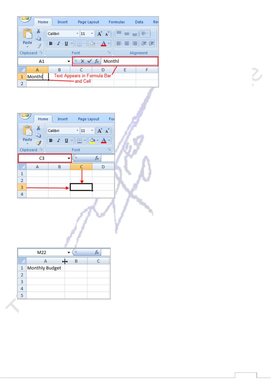
To Insert Text:
Left-click a cell to select it. Each rectangle in the worksheet is called a cell. As you select a cell, the
cell address appears in the Name Box.
Enter text into the cell using your keyboard. The text appears in the cell and in the formula bar.
111
Each cell has a name, or a cell address based on the column and row it is in. For example, this cell is C3
since it is where column C and row 3 intersect.
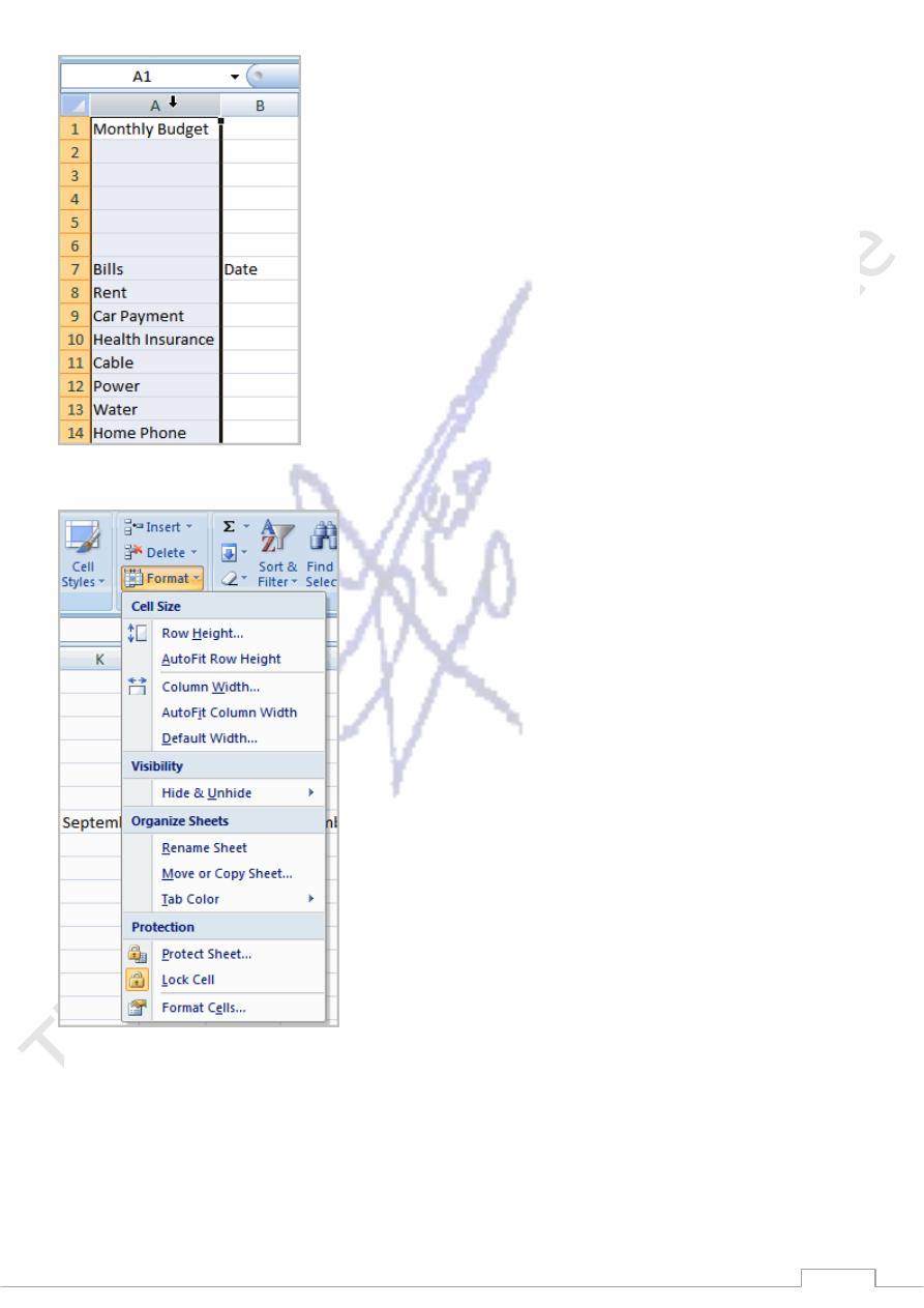
To Modify Column Width:
Position the cursor over the column line in the column heading and a double arrow will appear.
Left-click the mouse and drag the cursor to the right to increase the column width or to the left to
decrease the column width.
Release the mouse button.
OR
Left-click the column heading of a column you'd like to modify. The entire column will appear
highlighted.
112
Click the Format command in the Cells group on the Home tab. A menu will appear.
Select Column Width to enter a specific column measurement.
Select AutoFit Column Width to adjust the column so all the text will fit.
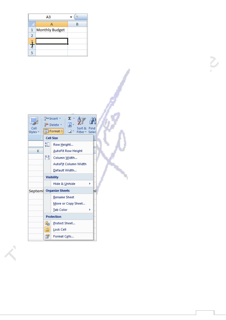
To Modify the Row Height:
Position the cursor over the row line you want to modify and a double arrow will appear.
113
Left-click the mouse and drag the cursor upward to decrease the row height or downward to
increase the row height.
Release the mouse button.
OR
Click the Format command in the Cells group on the Home tab. A menu will appear.
Select Row Height to enter a specific row measurement.
Select AutoFit Row Height to adjust the row so all the text will fit.
To Insert Rows:
Select the row below where you want the new row to appear.
Click the Insert command in the Cells group on the Home tab. The row will appear.
114
The new row always appears above the selected row.
Make sure that you select the entire row below where you want the new row to appear and not just the cell.
If you select just the cell and then click Insert, only a new cell will appear.
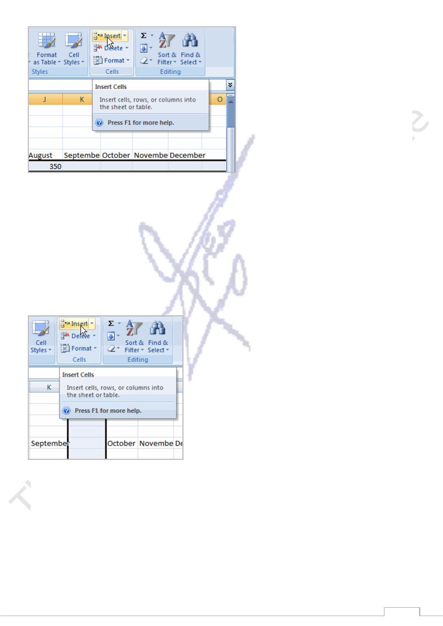
To Insert Columns:
Select the column to the right of where you want the column to appear.
Click the Insert command in the Cells group on the Home tab. The column will appear.
The new column always appears to the left of the selected column. For example, if you want to insert a
column between September and October, select the October column and click the Insert command.
Make sure that you select the entire column to the right of where you want the new column to appear and
not just the cell. If you select just the cell and then click Insert, only a new cell will appear.
To Delete Rows and Columns:
Select the row or column you’d like to delete.
Click the Delete command in the Cells group on the Home tab.
Formatting Cells
115
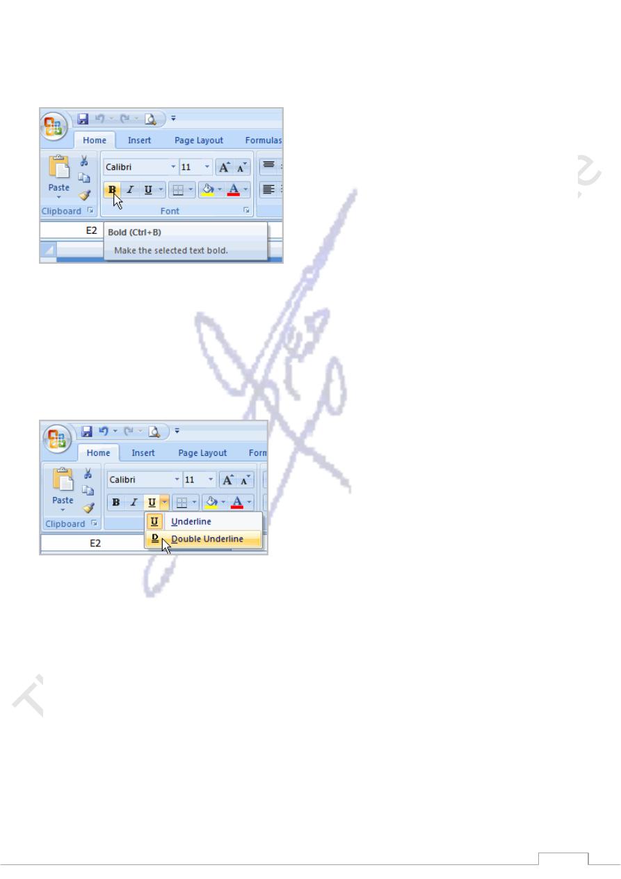
To Format Text in Bold or Italics:
Left-click a cell to select it or drag your cursor over the text in the formula bar to select it.
Click the Bold or Italics command.
You can select entire columns and rows, or specific cells. To select the entire column, just left-click the
column heading and the entire column will appear as selected. To select specific cells, just left-click a cell
and drag your mouse to select the other cells. Then, release the mouse button.
To Format Text as Underlined:
Select the cell or cells you want to format.
Click the drop-down arrow next to the Underline command.
Select the Single Underline or Double Underline option.
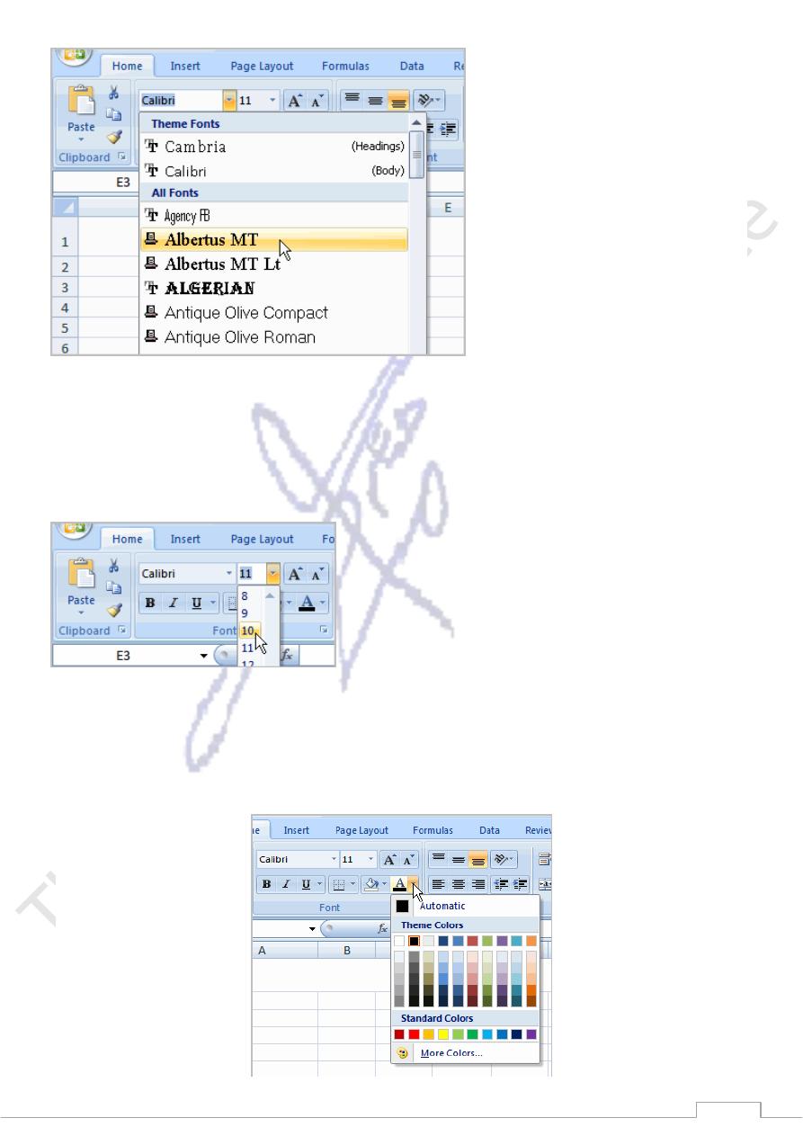
To Change the Font Style
Select the cell or cells you want to format.
Left-click the drop-down arrow next to the Font Style box on the Home tab.
Select a font style from the list.
116
As you move over the font list, the Live Preview feature previews the font for you in the spreadsheet.
To Change the Font Size:
Select the cell or cells you want to format.
Left-click the drop-down arrow next to the Font Size box on the Home tab.
Select a font size from the list.
To Change the Text Color:
Select the cell or cells you want to format.
Left-click the drop-down arrow next to the Text Color command. A color palette will appear.
Select a color from the palette.
117
OR
Select More Colors. A dialog box will appear.
Select a color.
Click OK.
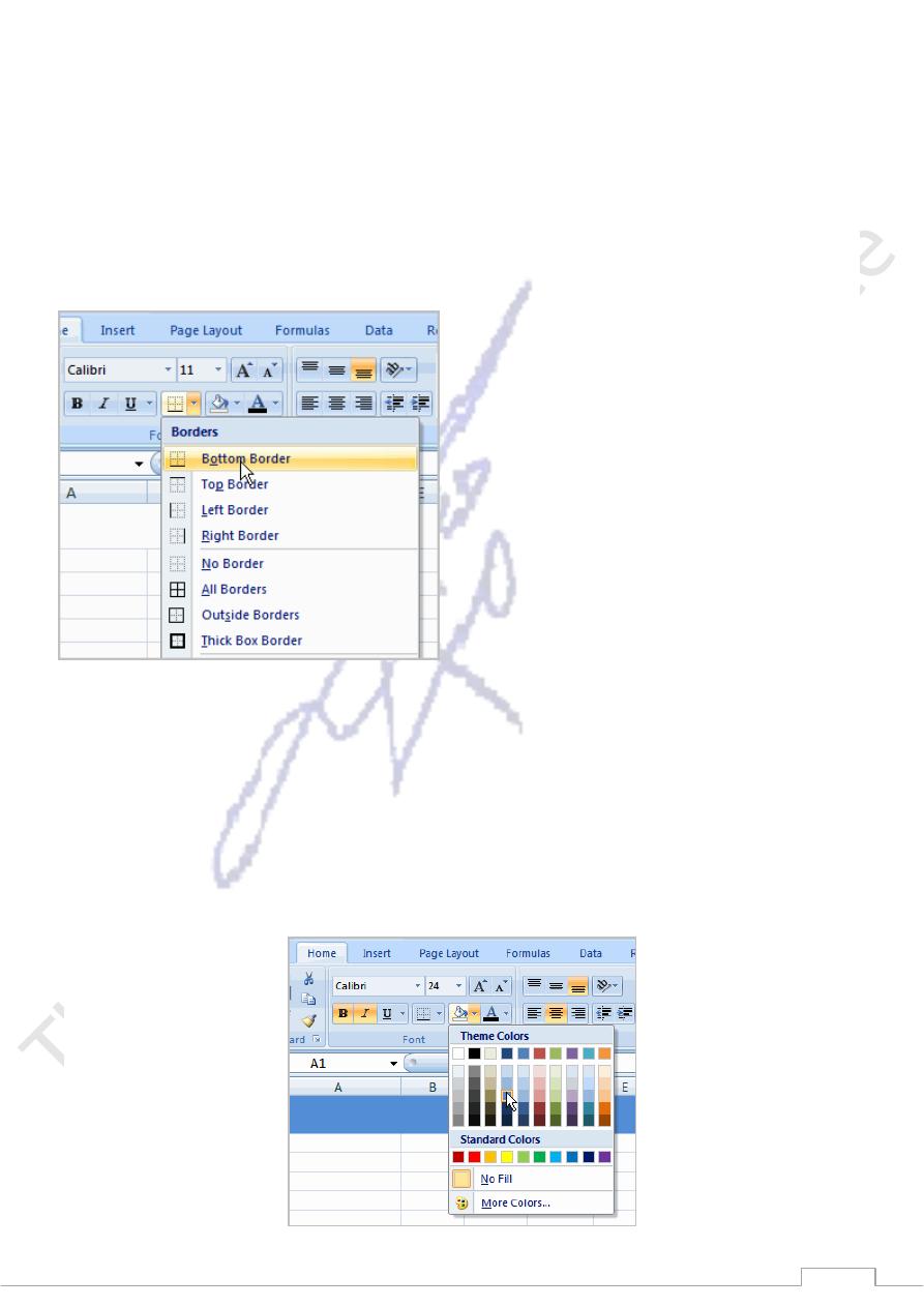
To Add a Border:
Select the cell or cells you want to format.
Click the drop-down arrow next to the Borders command on the Home tab. A menu will appear
with border options.
Left-click an option from the list to select it.
You can change the line style and color of the border.
To add a Fill Color:
Select the cell or cells you want to format.
Click the Fill command. A color palette will appear.
Select a color.

118
OR
Select More Colors. A dialog box will appear.
Select a color.
Click OK.
You can use the fill color feature to format columns and rows, and format a worksheet so that it is easier to
read.
To Format Numbers and Dates:
Select the cell or cells you want to format.
Left-click the drop-down arrow next to the Number Format box.
Select one of the options for formatting numbers.
By default, the numbers appear in the General category, which means there is no special formatting.
In the Number group, you have some other options. For example, you can change the U.S. dollar sign to
another currency format, numbers to percents, add commas, and change the decimal location.