First stage – College of Medicine – University of Mosul / Nineveh
Computer Science/2016-2017
Assistant Lecturer: Zina Abdul Salam
EXCEL 2013
LECTURE 2
1
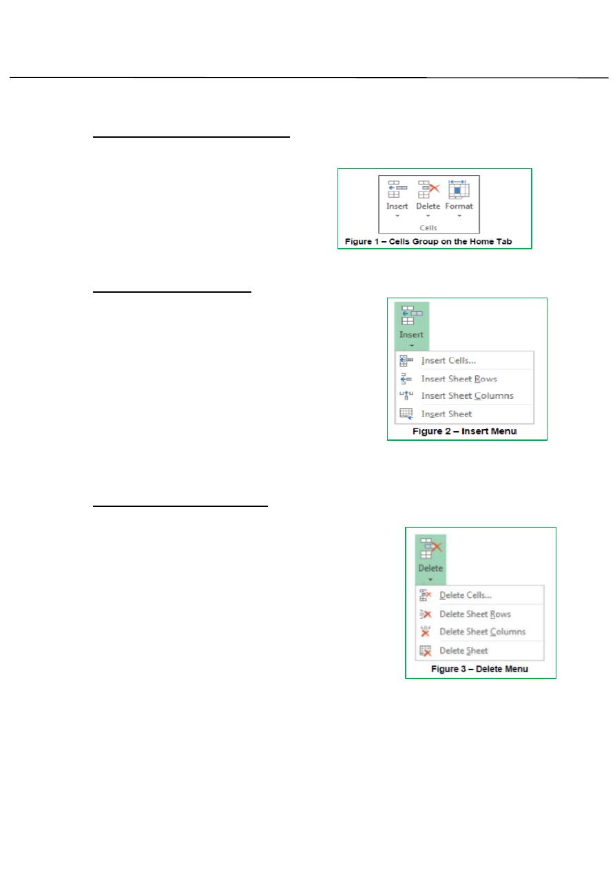
Working with Row and Columns:
Although the number of ROW and Columns is fixed, you can still insert
rows and column if you need to make
room for additional data, or delete rows
or column or hide them, from Home tab,
cell group there is commands can be
used.
Inserting Row and Column
To insert Row:
1. Select the row below where you want the new
row to appear.
2. Click the Insert command in the Cells group
on the Home tab. The row will appear.
To insert Column:
1. Select the column to the right of where you
want the column to appear.
2. Click the Insert command in the Cells group on the Home tab. The
column will appear.
Rows and Columns
Deleting
To delete Row:
1. Select the row that you want to delete.
2. From Home tab Insert command in the Cells
group
click delete sheet rows.
3. You can also delete row by right - clicking the
row header.
To delete column:
1. Select the Column that you want to delete
2. From Home tab Insert command in the Cells group click delete sheet
Column.
3. You can also delete Column by right - clicking the row header.
First stage – College of Medicine – University of Mosul / Nineveh
Computer Science/2016-2017
Assistant Lecturer: Zina Abdul Salam
EXCEL 2013
LECTURE 2
2
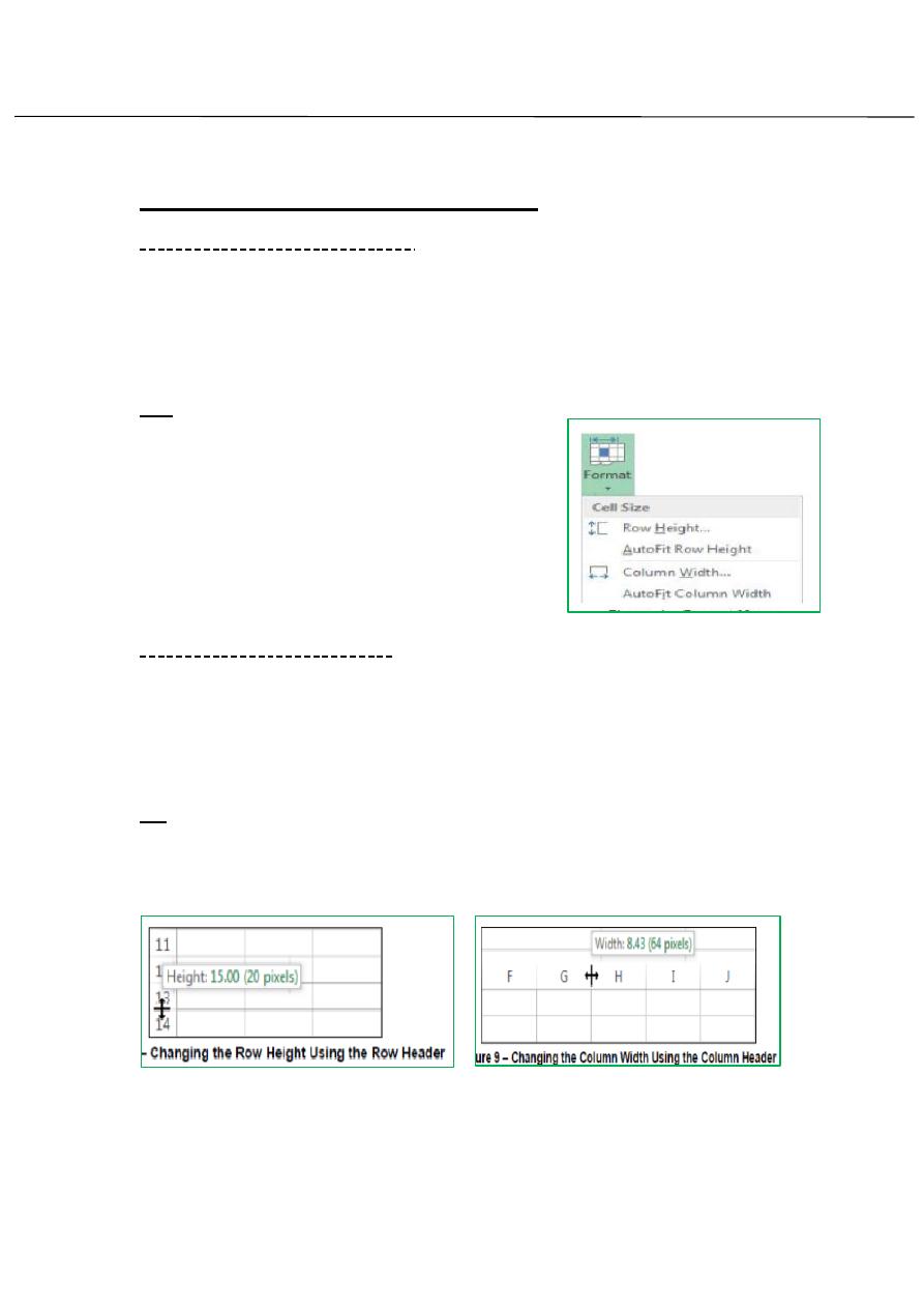
Modifying Columns, Rows and Cells
To change the Column Width:
1. Position the cursor over the column line in the column heading and a
double arrow will appear
2. Left-click the mouse and drag the cursor to the right to increase the
column width or to the left to decrease the column width.
3. Release the mouse button.
OR
1. Left-click the column heading of a column
you'd like to modify. The entire column will
appear highlighted.
2. Click the Format command in the Cells
group on the Home tab. A menu will appear.
3. Select AutoFit Column Width to adjust the
column so all the text will fit.
To change the Row Height:
1. Position the cursor over the row line you want to modify and a double
arrow will appear.
2. Left-click the mouse and drag the cursor upward to decrease the row
height or downward to Increase the row height.
3. Release the mouse button.
OR
a. Click the Format command in the Cells group on the Home tab. A
menu will appear.
b. Select AutoFit Row Height to adjust the row so all the text will fit.
First stage – College of Medicine – University of Mosul / Nineveh
Computer Science/2016-2017
Assistant Lecturer: Zina Abdul Salam
EXCEL 2013
LECTURE 2
3
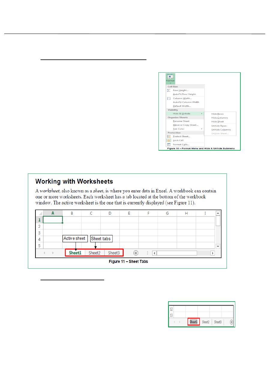
Hiding and Unhiding Rows and Columns:
You can hide rows and columns within a
worksheet.hidden rows and column do not
appear in a printout.
To hide a row or column:
1- Select the row or column you want to
hide.
2- On the home tab , in the Cell group,
click format button, point to
Hide&Unhide .
3- You can hide row & hide column by
right –clicking.
To rename a work sheet:
Renaming Worksheets:
1- Double –click the tab of the woksheet that you want to rename,
or right click the sheet tab and then click rename.
2- Type a new name, and press enter key.
3- Worksheet name can not exceed 31
characters and can not be blank ,each
worksheet name ina workbook must
be unique.
First stage – College of Medicine – University of Mosul / Nineveh
Computer Science/2016-2017
Assistant Lecturer: Zina Abdul Salam
EXCEL 2013
LECTURE 2
4
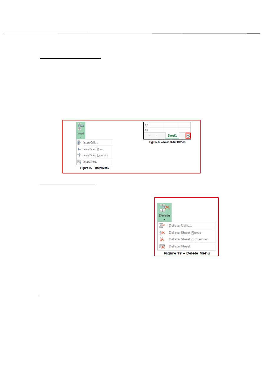
Inserting Worksheets: By default, each new workbook contains one
worksheet. You can insert additional worksheets as needed.
To insert a worksheet:
1- Click the tab of the work sheet to the left of which you want to
insert a new work sheet.
2- On Home tab , in the cells group, click the insert arrow, and then
click Insert Sheet (see figure 16).
Deleting Worksheets:
If you no longer need a worksheet, you can delete it from workbook.
Deleting a worksheet cannot be undone.
To delete a worksheet:
1- Click the tab of the worksheet that
you want to delete
2- On the Home tab, in the Cell group,
click Delete arrow , and then click
sheet.(see figure 18)
3- If the work sheet contains data, a dialog box opens asking you to
confirm. Click delete (see figure 19).
4- You can also delete worksheet by right.
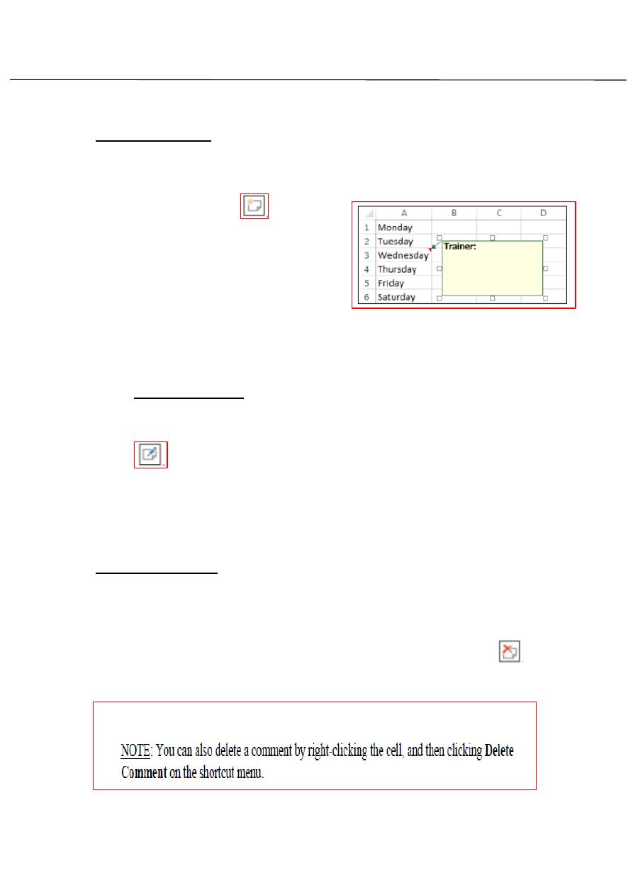
Adding Comments
You can add a comment to any cell in a work sheet. Excel label each
new comment by using a name that is specified in the Excel options
dialog box.
First stage – College of Medicine – University of Mosul / Nineveh
Computer Science/2016-2017
Assistant Lecturer: Zina Abdul Salam
EXCEL 2013
LECTURE 2
5
To add a comment:
1- Select the cell to which you want to add a comment.
2- On the Review tab, in the Comment group, click the new
Comment button
. Or right
click the cell, and then click Insert
Comment on the shortcut menu.
3- Type the comment in the
comment box.
4- When finished, click any cell in
the worksheet to hide the comment .A red triangle appears in the
upper-right corner of the cell to indicate that it contains a
comment.
To edit comment:
1- Select the cell that you want to edit comment from.
2- On review tab, in the comment group, click edit comment button
or, right –click the cell, and then click Edit Comment on the
shortcut menu.
3- Edit the comment in the comment box.
4- When finished, click any cell in the worksheet to hide the
comment
Deleting Comments
To delete comment that you are no longer needed:
1-Select the cell that you want to delete comment from.
2-On the Review tab, in the Comment group, click Delete button
.
First stage – College of Medicine – University of Mosul / Nineveh
Computer Science/2016-2017
Assistant Lecturer: Zina Abdul Salam
EXCEL 2013
LECTURE 2
6
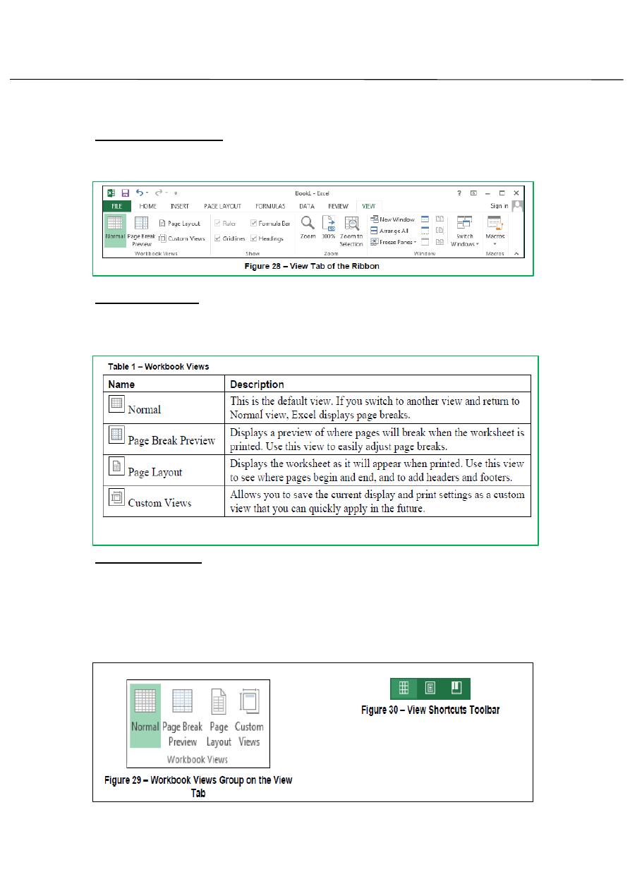
Working with Views:
Excel provides several ways in which you can view worksheets.
Switching Views:
Excel offers a variety of viewing that change how a worksheet is
displayed on the screen. (See table 1)
To switch Views:
1-On the View tab, in the Workbook Views group, click the desired view
button (see figure 29).
2- Or click the desired view button on View Shortcuts toolbar located on
the right side of the Statues bar (see figure 30).
First stage – College of Medicine – University of Mosul / Nineveh
Computer Science/2016-2017
Assistant Lecturer: Zina Abdul Salam
EXCEL 2013
LECTURE 2
7
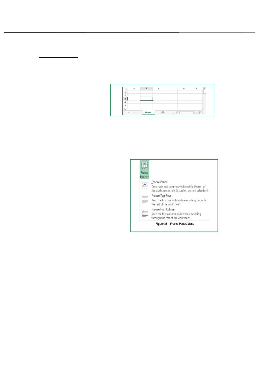
Freezing Panes:
Freezing Panes is a useful technique for keeping an area of a worksheet
Visible while you scroll to another area of the worksheet. You can freeze
only rows at the top and
column on the left side of
the worksheet, you cannot
freeze rows and columns
in the middle of the
worksheet. Excel displays dark gray lines to indicate frozen row and
column (see figure).
To freeze panes:
1-Select the cell below the row and
to the right of the column that you
want to freeze.
2- On the View tab, in the Window
group, click the Freeze panes
button, and then click Freeze Pane.
3- When any row or column are
frozen, the Freeze Panes option
changes to Unfreeze Pane.
First stage – College of Medicine – University of Mosul / Nineveh
Computer Science/2016-2017
Assistant Lecturer: Zina Abdul Salam
EXCEL 2013
LECTURE 2
8
First stage – College of Medicine – University of Mosul / Nineveh
Computer Science/2016-2017
Assistant Lecturer: Zina Abdul Salam
EXCEL 2013
LECTURE 2
9
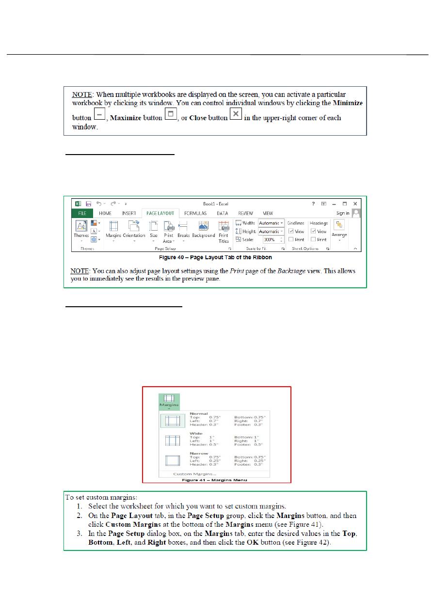
ayout
Changing the page L
The commands used to define the layout of a printed page are available
on the Page Layout tab of the Ribbon.
:
Changing the page margins
To change the page margins:
1-Select the work sheet for which you want to change the margins.
2- On the page layout tab, in the page setup group, click the Margins
button and select the desired margin setting from the menu.

First stage – College of Medicine – University of Mosul / Nineveh
Computer Science/2016-2017
Assistant Lecturer: Zina Abdul Salam
EXCEL 2013
LECTURE 2
11
Changing the Page Orientation:
In Excel, you can print a worksheet in either portrait or landscape
orientation.
To change the page orientation:
1-Select the work sheet for which you want to change the orientation.
2- On the page layout tab, in the page setup group, click the Margins
orientation button and then select the click either portrait or landscape.
Setting a print Area:
By default, Excel print the entire worksheet. If you frequently print a
specific section of worksheet. You can set a print area that includes just
that section. That way, when you print the worksheet, only that section
will print.
To set a print area:
1-Select the cells that you want to define as the print area.
2- On the page layout tab, in the page
setup group, click the print Area button and
then click set print Area.
3-You can clear the print area by clicking
the Print Area button, and then clicking
Clear Print Area.
First stage – College of Medicine – University of Mosul / Nineveh
Computer Science/2016-2017
Assistant Lecturer: Zina Abdul Salam
EXCEL 2013
LECTURE 2
11
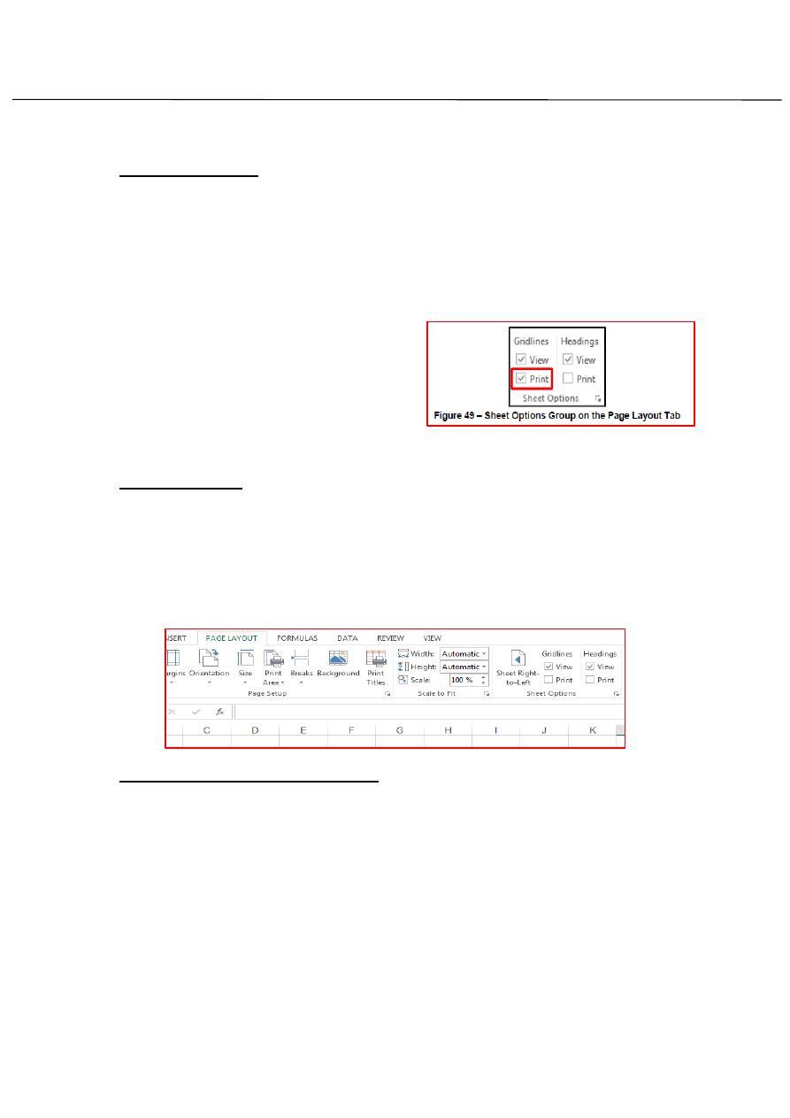
:
Printing Gridlines
Gridlines are the light gray lines that appear around cells in a
worksheet. By default, gridline are displayed on the screen, but they are
not printed. You can choose to print a worksheet with gridlines that
make the data easier to red on a printed page.
To print gridlines:
1- Select the worksheet that you
want to print with gridlines.
2- On the page layout tab, in the
sheet options group, under
gridlines, select the print check box.
Sheet direction:
Normally, the worksheet direction is Left-to-Right in Excel, but in order to
satisfy certain language writing habits from right to left, Excel can switch
direction of the worksheet which place the row and column heading on
right as following screenshots shown. From Page Layout tab, sheet option
click sheet Right to left.
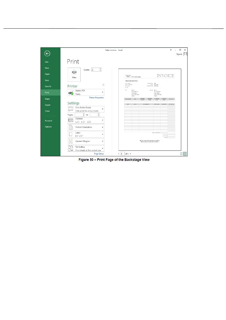
Previewing and print worksheets:
Before printing a worksheet, you can preview it to see how each page
Will look when printed. The print page of backstage view allows you to
preview a worksheet.
First stage – College of Medicine – University of Mosul / Nineveh
Computer Science/2016-2017
Assistant Lecturer: Zina Abdul Salam
EXCEL 2013
LECTURE 2
12
To preview and print a worksheet:
1- Select the worksheet that you want to preview and print.
2- Click the File tab, and then click Print, or press CTRL+P the print page
of the Backstage view opens, displaying print setting in the center pane
and preview of the worksheet in the right pane.