
Excerpts from this work may be reproduced by instructors for distribution on a not-for-profit basis for testing or instructional purposes only to
students enrolled in courses for which the textbook has been adopted. Any other reproduction or translation of this work beyond that permitted
by Sections 107 or 108 of the 1976 United States Copyright Act without the permission of the copyright owner is unlawful.
CHAPTER 2
ATOMIC STRUCTURE AND INTERATOMIC BONDING
PROBLEM SOLUTIONS
Fundamental Concepts
Electrons in Atoms
2.1 Cite the difference between atomic mass and atomic weight.
Solution
Atomic mass is the mass of an individual atom, whereas atomic weight is the average (weighted) of the
atomic masses of an atom's naturally occurring isotopes.

Excerpts from this work may be reproduced by instructors for distribution on a not-for-profit basis for testing or instructional purposes only to
students enrolled in courses for which the textbook has been adopted. Any other reproduction or translation of this work beyond that permitted
by Sections 107 or 108 of the 1976 United States Copyright Act without the permission of the copyright owner is unlawful.
2.2 Chromium has four naturally-occurring isotopes: 4.34% of
50
Cr, with an atomic weight of 49.9460
amu, 83.79% of
52
Cr, with an atomic weight of 51.9405 amu, 9.50% of
53
Cr, with an atomic weight of 52.9407 amu,
and 2.37% of
54
Cr, with an atomic weight of 53.9389 amu. On the basis of these data, confirm that the average
atomic weight of Cr is 51.9963 amu.
Solution
The average atomic weight of silicon
( A
Cr
) is computed by adding fraction-of-occurrence/atomic weight
products for the three isotopes. Thus
A
Cr
= f
50Cr
A
50Cr
+ f
52Cr
A
52Cr
+ f
53Cr
A
53Cr
+ f
54Cr
A
54Cr
= (0.0434)(49.9460 amu) + (0.8379)(51.9405 amu) + (0.0950)(52.9407 amu) + (0.0237)(53.9389 amu) = 51.9963 amu

Excerpts from this work may be reproduced by instructors for distribution on a not-for-profit basis for testing or instructional purposes only to
students enrolled in courses for which the textbook has been adopted. Any other reproduction or translation of this work beyond that permitted
by Sections 107 or 108 of the 1976 United States Copyright Act without the permission of the copyright owner is unlawful.
2.3
(a) How many grams are there in one amu of a material?
(b) Mole, in the context of this book, is taken in units of gram-mole. On this basis, how many atoms
are there in a pound-mole of a substance?
Solution
(a) In order to determine the number of grams in one amu of material, appropriate manipulation of the
amu/atom, g/mol, and atom/mol relationships is all that is necessary, as
# g/amu =
1 mol
6.022
× 10
23
atoms
1 g / mol
1 amu / atom
= 1.66
× 10
-24
g/amu
(b) Since there are 453.6 g/lb
m
,
1 lb - mol = (453.6 g/lb
m
) (6.022
× 10
23
atoms/g - mol)
= 2.73
× 10
26
atoms/lb-mol

Excerpts from this work may be reproduced by instructors for distribution on a not-for-profit basis for testing or instructional purposes only to
students enrolled in courses for which the textbook has been adopted. Any other reproduction or translation of this work beyond that permitted
by Sections 107 or 108 of the 1976 United States Copyright Act without the permission of the copyright owner is unlawful.
2.4 (a) Cite two important quantum-mechanical concepts associated with the Bohr model of the atom.
(b) Cite two important additional refinements that resulted from the wave-mechanical atomic model.
Solution
(a) Two important quantum-mechanical concepts associated with the Bohr model of the atom are (1) that
electrons are particles moving in discrete orbitals, and (2) electron energy is quantized into shells.
(b) Two important refinements resulting from the wave-mechanical atomic model are (1) that electron
position is described in terms of a probability distribution, and (2) electron energy is quantized into both shells and
subshells--each electron is characterized by four quantum numbers.

Excerpts from this work may be reproduced by instructors for distribution on a not-for-profit basis for testing or instructional purposes only to
students enrolled in courses for which the textbook has been adopted. Any other reproduction or translation of this work beyond that permitted
by Sections 107 or 108 of the 1976 United States Copyright Act without the permission of the copyright owner is unlawful.
2.5 Relative to electrons and electron states, what does each of the four quantum numbers specify?
Solution
The n quantum number designates the electron shell.
The l quantum number designates the electron subshell.
The m
l
quantum number designates the number of electron states in each electron subshell.
The m
s
quantum number designates the spin moment on each electron.

Excerpts from this work may be reproduced by instructors for distribution on a not-for-profit basis for testing or instructional purposes only to
students enrolled in courses for which the textbook has been adopted. Any other reproduction or translation of this work beyond that permitted
by Sections 107 or 108 of the 1976 United States Copyright Act without the permission of the copyright owner is unlawful.
2.6
Allowed values for the quantum numbers of electrons are as follows:
n = 1, 2, 3, . . .
l = 0, 1, 2, 3, . . . , n –1
m
l
= 0, ±1, ±2, ±3, . . . , ±l
m
s
=
±
1
2
The relationships between n and the shell designations are noted in Table 2.1. Relative to the subshells,
l = 0 corresponds to an s subshell
l = 1 corresponds to a p subshell
l = 2 corresponds to a d subshell
l = 3 corresponds to an f subshell
For the K shell, the four quantum numbers for each of the two electrons in the 1s state, in the order of nlm
l
m
s
, are
100(
1
2
) and 100(
−
1
2
). Write the four quantum numbers for all of the electrons in the L and M shells, and note
which correspond to the s, p, and d subshells.
Solution
For the L state, n = 2, and eight electron states are possible. Possible l values are 0 and 1, while possible m
l
values are 0 and ±1; and possible m
s
values are
±
1
2
.
Therefore, for the s states, the quantum numbers are
200
(
1
2
)
and
200
(
−
1
2
)
. For the p states, the quantum numbers are
210
(
1
2
)
,
210
(
−
1
2
)
,
211
(
1
2
)
,
211
(
−
1
2
)
,
21 (
−
1)
(
1
2
)
, and
21 (
−
1)
(
−
1
2
)
.
For the M state, n = 3, and 18 states are possible. Possible l values are 0, 1, and 2; possible m
l
values are
0, ±1, and ±2; and possible m
s
values are
±
1
2
.
Therefore, for the s states, the quantum numbers are
300
(
1
2
)
,
300
(
−
1
2
)
, for the p states they are
310
(
1
2
)
,
310
(
−
1
2
)
,
311
(
1
2
)
,
311
(
−
1
2
)
,
31 (
−
1)
(
1
2
)
, and
31 (
−
1)
(
−
1
2
)
; for the d
states they are
320
(
1
2
)
,
320
(
−
1
2
)
,
321
(
1
2
)
,
321
(
−
1
2
)
,
32 (
−
1)
(
1
2
)
,
32 (
−
1)
(
−
1
2
)
,
322
(
1
2
)
,
322
(
−
1
2
)
,
32 (
−
2)
(
1
2
)
,
and
32 (
−
2)
(
−
1
2
)
.

Excerpts from this work may be reproduced by instructors for distribution on a not-for-profit basis for testing or instructional purposes only to
students enrolled in courses for which the textbook has been adopted. Any other reproduction or translation of this work beyond that permitted
by Sections 107 or 108 of the 1976 United States Copyright Act without the permission of the copyright owner is unlawful.
2.7 Give the electron configurations for the following ions: Fe
2+
, Al
3+
, Cu
+
, Ba
2+
, Br
-
, and O
2-
.
Solution
The electron configurations for the ions are determined using Table 2.2 (and Figure 2.6).
Fe
2+
: From Table 2.2, the electron configuration for an atom of iron is 1s
2
2s
2
2p
6
3s
2
3p
6
3d
6
4s
2
. In order to
become an ion with a plus two charge, it must lose two electrons—in this case the two 4s. Thus, the electron
configuration for an Fe
2+
ion is 1s
2
2s
2
2p
6
3s
2
3p
6
3d
6
.
Al
3+
: From Table 2.2, the electron configuration for an atom of aluminum is 1s
2
2s
2
2p
6
3s
2
3p
1
. In order to
become an ion with a plus three charge, it must lose three electrons—in this case two 3s and the one 3p. Thus, the
electron configuration for an Al
3+
ion is 1s
2
2s
2
2p
6
.
Cu
+
: From Table 2.2, the electron configuration for an atom of copper is 1s
2
2s
2
2p
6
3s
2
3p
6
3d
10
4s
1
. In order
to become an ion with a plus one charge, it must lose one electron—in this case the 4s. Thus, the electron
configuration for a Cu
+
ion is 1s
2
2s
2
2p
6
3s
2
3p
6
3d
10
.
Ba
2+
: The atomic number for barium is 56 (Figure 2.6), and inasmuch as it is not a transition element the
electron configuration for one of its atoms is 1s
2
2s
2
2p
6
3s
2
3p
6
3d
10
4s
2
4p
6
4d
10
5s
2
5p
6
6s
2
. In order to become an ion
with a plus two charge, it must lose two electrons—in this case two the 6s. Thus, the electron configuration for a
Ba
2+
ion is 1s
2
2s
2
2p
6
3s
2
3p
6
3d
10
4s
2
4p
6
4d
10
5s
2
5p
6
.
Br
-
: From Table 2.2, the electron configuration for an atom of bromine is 1s
2
2s
2
2p
6
3s
2
3p
6
3d
10
4s
2
4p
5
. In
order to become an ion with a minus one charge, it must acquire one electron—in this case another 4p. Thus, the
electron configuration for a Br
-
ion is 1s
2
2s
2
2p
6
3s
2
3p
6
3d
10
4s
2
4p
6
.
O
2-
: From Table 2.2, the electron configuration for an atom of oxygen is 1s
2
2s
2
2p
4
. In order to become an
ion with a minus two charge, it must acquire two electrons—in this case another two 2p. Thus, the electron
configuration for an O
2-
ion is 1s
2
2s
2
2p
6
.

Excerpts from this work may be reproduced by instructors for distribution on a not-for-profit basis for testing or instructional purposes only to
students enrolled in courses for which the textbook has been adopted. Any other reproduction or translation of this work beyond that permitted
by Sections 107 or 108 of the 1976 United States Copyright Act without the permission of the copyright owner is unlawful.
2.8 Sodium chloride (NaCl) exhibits predominantly ionic bonding. The Na
+
and Cl
-
ions have electron
structures that are identical to which two inert gases?
Solution
The Na
+
ion is just a sodium atom that has lost one electron; therefore, it has an electron configuration the
same as neon (Figure 2.6).
The Cl
-
ion is a chlorine atom that has acquired one extra electron; therefore, it has an electron
configuration the same as argon.

Excerpts from this work may be reproduced by instructors for distribution on a not-for-profit basis for testing or instructional purposes only to
students enrolled in courses for which the textbook has been adopted. Any other reproduction or translation of this work beyond that permitted
by Sections 107 or 108 of the 1976 United States Copyright Act without the permission of the copyright owner is unlawful.
The Periodic Table
2.9 With regard to electron configuration, what do all the elements in Group VIIA of the periodic table
have in common?
Solution
Each of the elements in Group VIIA has five p electrons.

Excerpts from this work may be reproduced by instructors for distribution on a not-for-profit basis for testing or instructional purposes only to
students enrolled in courses for which the textbook has been adopted. Any other reproduction or translation of this work beyond that permitted
by Sections 107 or 108 of the 1976 United States Copyright Act without the permission of the copyright owner is unlawful.
2.10 To what group in the periodic table would an element with atomic number 114 belong?
Solution
From the periodic table (Figure 2.6) the element having atomic number 114 would belong to group IVA.
According to Figure 2.6, Ds, having an atomic number of 110 lies below Pt in the periodic table and in the right-
most column of group VIII. Moving four columns to the right puts element 114 under Pb and in group IVA.

Excerpts from this work may be reproduced by instructors for distribution on a not-for-profit basis for testing or instructional purposes only to
students enrolled in courses for which the textbook has been adopted. Any other reproduction or translation of this work beyond that permitted
by Sections 107 or 108 of the 1976 United States Copyright Act without the permission of the copyright owner is unlawful.
2.11 Without consulting Figure 2.6 or Table 2.2, determine whether each of the electron configurations
given below is an inert gas, a halogen, an alkali metal, an alkaline earth metal, or a transition metal. Justify your
choices.
(a) 1s
2
2s
2
2p
6
3s
2
3p
6
3d
7
4s
2
(b) 1s
2
2s
2
2p
6
3s
2
3p
6
(c) 1s
2
2s
2
2p
5
(d) 1s
2
2s
2
2p
6
3s
2
(e) 1s
2
2s
2
2p
6
3s
2
3p
6
3d
2
4s
2
(f) 1s
2
2s
2
2p
6
3s
2
3p
6
4s
1
Solution
(a) The 1s
2
2s
2
2p
6
3s
2
3p
6
3d
7
4s
2
electron configuration is that of a transition metal because of an incomplete
d subshell.
(b) The 1s
2
2s
2
2p
6
3s
2
3p
6
electron configuration is that of an inert gas because of filled 3s and 3p subshells.
(c) The 1s
2
2s
2
2p
5
electron configuration is that of a halogen because it is one electron deficient from
having a filled L shell.
(d) The 1s
2
2s
2
2p
6
3s
2
electron configuration is that of an alkaline earth metal because of two s electrons.
(e) The 1s
2
2s
2
2p
6
3s
2
3p
6
3d
2
4s
2
electron configuration is that of a transition metal because of an incomplete
d subshell.
(f) The 1s
2
2s
2
2p
6
3s
2
3p
6
4s
1
electron configuration is that of an alkali metal because of a single s electron.

Excerpts from this work may be reproduced by instructors for distribution on a not-for-profit basis for testing or instructional purposes only to
students enrolled in courses for which the textbook has been adopted. Any other reproduction or translation of this work beyond that permitted
by Sections 107 or 108 of the 1976 United States Copyright Act without the permission of the copyright owner is unlawful.
2.12 (a) What electron subshell is being filled for the rare earth series of elements on the periodic table?
(b) What electron subshell is being filled for the actinide series?
Solution
(a) The 4f subshell is being filled for the rare earth series of elements.
(b) The 5f subshell is being filled for the actinide series of elements.

Excerpts from this work may be reproduced by instructors for distribution on a not-for-profit basis for testing or instructional purposes only to
students enrolled in courses for which the textbook has been adopted. Any other reproduction or translation of this work beyond that permitted
by Sections 107 or 108 of the 1976 United States Copyright Act without the permission of the copyright owner is unlawful.
Bonding Forces and Energies
2.13 Calculate the force of attraction between a K
+
and an O
2-
ion the centers of which are separated by a
distance of 1.5 nm.
Solution
The attractive force between two ions F
A
is just the derivative with respect to the interatomic separation of
the attractive energy expression, Equation 2.8, which is just
F
A
=
dE
A
dr
=
d
−
A
r
dr
=
A
r
2
The constant A in this expression is defined in footnote 3. Since the valences of the K
+
and O
2
- ions (Z
1
and Z
2
) are
+1 and -2, respectively, Z
1
= 1 and Z
2
= 2, then
F
A
=
(Z
1
e) (Z
2
e)
4
πε
0
r
2
=
(1)(2 )
(
1.602
× 10
−19
C
)
2
(4)(
π) (8.85 × 10
−12
F/m) (1.5
× 10
−9
m)
2
= 2.05
× 10
-10
N
Excerpts from this work may be reproduced by instructors for distribution on a not-for-profit basis for testing or instructional purposes only to
students enrolled in courses for which the textbook has been adopted. Any other reproduction or translation of this work beyond that permitted
by Sections 107 or 108 of the 1976 United States Copyright Act without the permission of the copyright owner is unlawful.
2.14 The net potential energy between two adjacent ions, E
N
, may be represented by the sum of Equations
2.8 and 2.9; that is,
E
N
=
−
A
r
+
B
r
n
Calculate the bonding energy E
0
in terms of the parameters A, B, and n using the following procedure:
1. Differentiate E
N
with respect to r, and then set the resulting expression equal to zero, since the curve of
E
N
versus r is a minimum at E
0
.
2. Solve for r in terms of A, B, and n, which yields r
0
, the equilibrium interionic spacing.
3. Determine the expression for E
0
by substitution of r
0
into Equation 2.11.
Solution
(a) Differentiation of Equation 2.11 yields
dE
N
dr
=
d
−
A
r
dr
+
d
B
r
n
dr
=
A
r
(1 + 1)
−
nB
r
(n + 1)
= 0
(b) Now, solving for r (= r
0
)
A
r
0
2
=
nB
r
0
(n + 1)
or
r
0
=
A
nB
1/(1 - n)
(c) Substitution for r
0
into Equation 2.11 and solving for E (= E
0
)
E
0
=
−
A
r
0
+
B
r
0
n
=
−
A
A
nB
1/(1 - n)
+
B
A
nB
n/(1 - n)
Excerpts from this work may be reproduced by instructors for distribution on a not-for-profit basis for testing or instructional purposes only to
students enrolled in courses for which the textbook has been adopted. Any other reproduction or translation of this work beyond that permitted
by Sections 107 or 108 of the 1976 United States Copyright Act without the permission of the copyright owner is unlawful.
2.15 For a K
+
–Cl
–
ion pair, attractive and repulsive energies E
A
and E
R
, respectively, depend on the
distance between the ions r, according to
E
A
= −
1.436
r
E
R
=
5.8
× 10
−6
r
9
For these expressions, energies are expressed in electron volts per K
+
–Cl
–
pair, and r is the distance in nanometers.
The net energy E
N
is just the sum of the two expressions above.
(a) Superimpose on a single plot E
N
, E
R
, and E
A
versus r up to 1.0 nm.
(b) On the basis of this plot, determine (i) the equilibrium spacing r
0
between the K
+
and Cl
–
ions, and (ii)
the magnitude of the bonding energy E
0
between the two ions.
(c) Mathematically determine the r
0
and E
0
values using the solutions to Problem 2.14 and compare these
with the graphical results from part (b).
Solution
(a) Curves of E
A
, E
R
, and E
N
are shown on the plot below.
(b) From this plot
r
0
= 0.28 nm
E
0
= – 4.6 eV
Excerpts from this work may be reproduced by instructors for distribution on a not-for-profit basis for testing or instructional purposes only to
students enrolled in courses for which the textbook has been adopted. Any other reproduction or translation of this work beyond that permitted
by Sections 107 or 108 of the 1976 United States Copyright Act without the permission of the copyright owner is unlawful.
(c) From Equation 2.11 for E
N
A = 1.436
B = 5.86
× 10
-6
n = 9
Thus,
r
0
=
A
nB
1/(1 - n)
=
1.436
(8)
(
5.86
× 10
-6
)
1/(1 - 9)
= 0.279 nm
and
E
0
=
−
A
A
nB
1/(1 - n)
+
B
A
nB
n/(1 - n)
=
−
1.436
1.436
(9)
(
5.86
×
10
−6
)
1/(1
− 9)
+
5.86
× 10
−6
1.436
(9)
(
5.86
× 10
−6
)
9 /(1
− 9)
= – 4.57 eV
Excerpts from this work may be reproduced by instructors for distribution on a not-for-profit basis for testing or instructional purposes only to
students enrolled in courses for which the textbook has been adopted. Any other reproduction or translation of this work beyond that permitted
by Sections 107 or 108 of the 1976 United States Copyright Act without the permission of the copyright owner is unlawful.
2.16 Consider a hypothetical X
+
-Y
-
ion pair for which the equilibrium interionic spacing and bonding
energy values are 0.35 nm and -6.13 eV, respectively. If it is known that n in Equation 2.11 has a value of 10, using
the results of Problem 2.14, determine explicit expressions for attractive and repulsive energies E
A
and E
R
of
Equations 2.8 and 2.9.
Solution
This problem gives us, for a hypothetical X+-Y- ion pair, values for r
0
(0.35 nm), E
0
(– 6.13 eV), and n
(10), and asks that we determine explicit expressions for attractive and repulsive energies of Equations 2.8 and 2.9.
In essence, it is necessary to compute the values of A and B in these equations. Expressions for r
0
and E
0
in terms
of n, A, and B were determined in Problem 2.14, which are as follows:
r
0
=
A
nB
1/(1 - n)
E
0
=
−
A
A
nB
1/(1 - n)
+
B
A
nB
n/(1 - n)
Thus, we have two simultaneous equations with two unknowns (viz. A and B). Upon substitution of values for r
0
and E
0
in terms of n, these equations take the forms
0.35 nm =
A
10 B
1/(1 - 10)
=
A
10 B
-1/9
and
− 6.13 eV = −
A
A
10 B
1/(1
− 10)
+
B
A
10 B
10 /(1
− 10)
=
−
A
A
10B
−1/ 9
+
B
A
10B
−10 / 9
We now want to solve these two equations simultaneously for values of A and B. From the first of these two
equations, solving for A/8B leads to
Excerpts from this work may be reproduced by instructors for distribution on a not-for-profit basis for testing or instructional purposes only to
students enrolled in courses for which the textbook has been adopted. Any other reproduction or translation of this work beyond that permitted
by Sections 107 or 108 of the 1976 United States Copyright Act without the permission of the copyright owner is unlawful.
A
10B
= (0.35 nm)
-9
Furthermore, from the above equation the A is equal to
A = 10B(0.35 nm)
-9
When the above two expressions for A/10B and A are substituted into the above expression for E
0
(- 6.13 eV), the
following results
−6.13 eV = = −
A
A
10B
−1/ 9
+
B
A
10B
−10 / 9
=
−
10B(0.35 nm)
-9
(0.35 nm)
-9
[
]
−1/ 9
+
B
(0.35 nm)
-9
[
]
−10 / 9
=
−
10B(0.35 nm)
-9
0.35 nm
+
B
(0.35 nm)
10
Or
−6.13 eV = = −
10B
(0.35 nm)
10
+
B
(0.35 nm)
10
=
−
9B
(0.35 nm)
10
Solving for B from this equation yields
B = 1.88
× 10
-5
eV - nm
10
Furthermore, the value of A is determined from one of the previous equations, as follows:
A = 10B(0.35 nm)
-9
= (10)
(
1.88
× 10
-5
eV - nm
10
)
(0.35 nm)
-9
= 2.39 eV- nm
Thus, Equations 2.8 and 2.9 become

Excerpts from this work may be reproduced by instructors for distribution on a not-for-profit basis for testing or instructional purposes only to
students enrolled in courses for which the textbook has been adopted. Any other reproduction or translation of this work beyond that permitted
by Sections 107 or 108 of the 1976 United States Copyright Act without the permission of the copyright owner is unlawful.
E
A
=
−
2.39
r
E
R
=
1.88
× 10
−5
r
10
Of course these expressions are valid for r and E in units of nanometers and electron volts, respectively.

Excerpts from this work may be reproduced by instructors for distribution on a not-for-profit basis for testing or instructional purposes only to
students enrolled in courses for which the textbook has been adopted. Any other reproduction or translation of this work beyond that permitted
by Sections 107 or 108 of the 1976 United States Copyright Act without the permission of the copyright owner is unlawful.
2.17
The net potential energy E
N
between two adjacent ions is sometimes represented by the expression
E
N
= −
C
r
+ DÊexp −
r
ρ
(2.12)
in which r is the interionic separation an
d C, D, and ρ are constants whose values depend on the specific material.
(a) Derive an expression for the bonding energy E
0
in terms of the equilibrium interionic separation r
0
and
the constants D and ρ using the following procedure:
1. Differentiate E
N
with respect to r and set the resulting expression equal to zero.
2. Solve for C in terms of D, ρ, and r
0
.
3. Determine the expression for E
0
by substitution for C in Equation 2.12.
(b) Derive another expression for E
0
in terms of r
0
, C, and ρ using a procedure analogous to the one
outlined in part (a).
Solution
(a) Differentiating Equation 2.12 with respect to r yields
dE
dr
=
d
−
C
r
dr
−
d D exp
−
r
ρ
dr
=
C
r
2
−
De
− r /ρ
ρ
At r = r
0
, dE/dr = 0, and
C
r
0
2
=
De
−(r
0
/
ρ)
ρ
(2.12b)
Solving for C and substitution into Equation 2.12 yields an expression for E
0
as
E
0
= De
−(r
0
/
ρ)
1
−
r
0
ρ
(b) Now solving for D from Equation 2.12b above yields
D =
C
ρ e
(r
0
/
ρ)
r
0
2

Excerpts from this work may be reproduced by instructors for distribution on a not-for-profit basis for testing or instructional purposes only to
students enrolled in courses for which the textbook has been adopted. Any other reproduction or translation of this work beyond that permitted
by Sections 107 or 108 of the 1976 United States Copyright Act without the permission of the copyright owner is unlawful.
Substitution of this expression for D into Equation 2.12 yields an expression for E
0
as
E
0
=
C
r
0
ρ
r
0
− 1

Excerpts from this work may be reproduced by instructors for distribution on a not-for-profit basis for testing or instructional purposes only to
students enrolled in courses for which the textbook has been adopted. Any other reproduction or translation of this work beyond that permitted
by Sections 107 or 108 of the 1976 United States Copyright Act without the permission of the copyright owner is unlawful.
Primary Interatomic Bonds
2.18 (a) Briefly cite the main differences between ionic, covalent, and metallic bonding.
(b) State the Pauli exclusion principle.
Solution
(a) The main differences between the various forms of primary bonding are:
Ionic--there is electrostatic attraction between oppositely charged ions.
Covalent--there is electron sharing between two adjacent atoms such that each atom assumes a
stable electron configuration.
Metallic--the positively charged ion cores are shielded from one another, and also "glued"
together by the sea of valence electrons.
(b) The Pauli exclusion principle states that each electron state can hold no more than two electrons, which
must have opposite spins.

Excerpts from this work may be reproduced by instructors for distribution on a not-for-profit basis for testing or instructional purposes only to
students enrolled in courses for which the textbook has been adopted. Any other reproduction or translation of this work beyond that permitted
by Sections 107 or 108 of the 1976 United States Copyright Act without the permission of the copyright owner is unlawful.
2.19 Compute the percents ionic character of the interatomic bonds for the following compounds: TiO
2
,
ZnTe, CsCl, InSb, and MgCl
2
.
Solution
The percent ionic character is a function of the electron negativities of the ions X
A
and X
B
according to
Equation 2.10. The electronegativities of the elements are found in Figure 2.7.
For TiO
2
, X
Ti
= 1.5 and X
O
= 3.5, and therefore,
%IC = 1
− e
(
− 0.25)(3.5−1.5)2
× 100 = 63.2%
For ZnTe, X
Zn
= 1.6 and X
Te
= 2.1, and therefore,
%IC = 1
− e
(
−0.25)(2.1−1.6)2
× 100 = 6.1%
For CsCl, X
Cs
= 0.7 and X
Cl
= 3.0, and therefore,
%IC = 1
− e
(
− 0.25)(3.0− 0.7)2
× 100 = 73.4%
For InSb, X
In
= 1.7 and X
Sb
= 1.9, and therefore,
%IC = 1
− e
(
− 0.25)(1.9−1.7)2
× 100 = 1.0%
For MgCl
2
, X
Mg
= 1.2 and X
Cl
= 3.0, and therefore,
%IC = 1
− e
(
− 0.25)(3.0−1.2)2
× 100 = 55.5%
Excerpts from this work may be reproduced by instructors for distribution on a not-for-profit basis for testing or instructional purposes only to
students enrolled in courses for which the textbook has been adopted. Any other reproduction or translation of this work beyond that permitted
by Sections 107 or 108 of the 1976 United States Copyright Act without the permission of the copyright owner is unlawful.
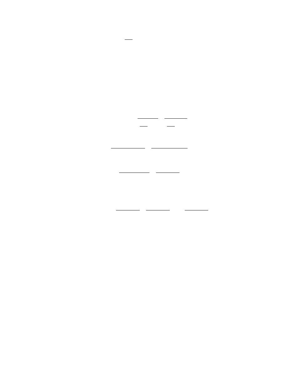
2.20 Make a plot of bonding energy versus melting temperature for the metals listed in Table 2.3. Using
this plot, approximate the bonding energy for copper, which has a melting temperature of 1084
°C.
Solution
Below is plotted the bonding energy versus melting temperature for these four metals. From this plot, the
bonding energy for copper (melting temperature of 1084
°C) should be approximately 3.6 eV. The experimental
value is 3.5 eV.

Excerpts from this work may be reproduced by instructors for distribution on a not-for-profit basis for testing or instructional purposes only to
students enrolled in courses for which the textbook has been adopted. Any other reproduction or translation of this work beyond that permitted
by Sections 107 or 108 of the 1976 United States Copyright Act without the permission of the copyright owner is unlawful.
2.21 Using Table 2.2, determine the number of covalent bonds that are possible for atoms of the following
elements: germanium, phosphorus, selenium, and chlorine.
Solution
For germanium, having the valence electron structure 4s
2
4p
2
, N' = 4; thus, there are 8 – N' = 4 covalent
bonds per atom.
For phosphorus, having the valence electron structure 3s
2
3p
3
, N' = 5; thus, there is 8 – N' = 3 covalent
bonds per atom.
For selenium, having the valence electron structure 4s
2
4p
4
, N' = 6; thus, there are 8 – N' = 2 covalent
bonds per atom.
For chlorine, having the valence electron structure 3s
2
3p
5
, N' = 7; thus, there are 8 – N' = 1 covalent bond
per atom.

Excerpts from this work may be reproduced by instructors for distribution on a not-for-profit basis for testing or instructional purposes only to
students enrolled in courses for which the textbook has been adopted. Any other reproduction or translation of this work beyond that permitted
by Sections 107 or 108 of the 1976 United States Copyright Act without the permission of the copyright owner is unlawful.
2.22 What type(s) of bonding would be expected for each of the following materials: brass (a copper-zinc
alloy), rubber, barium sulfide (BaS), solid xenon, bronze, nylon, and aluminum phosphide (AlP)?
Solution
For brass, the bonding is metallic since it is a metal alloy.
For rubber, the bonding is covalent with some van der Waals. (Rubber is composed primarily of carbon
and hydrogen atoms.)
For BaS, the bonding is predominantly ionic (but with some covalent character) on the basis of the relative
positions of Ba and S in the periodic table.
For solid xenon, the bonding is van der Waals since xenon is an inert gas.
For bronze, the bonding is metallic since it is a metal alloy (composed of copper and tin).
For nylon, the bonding is covalent with perhaps some van der Waals. (Nylon is composed primarily of
carbon and hydrogen.)
For AlP the bonding is predominantly covalent (but with some ionic character) on the basis of the relative
positions of Al and P in the periodic table.

Excerpts from this work may be reproduced by instructors for distribution on a not-for-profit basis for testing or instructional purposes only to
students enrolled in courses for which the textbook has been adopted. Any other reproduction or translation of this work beyond that permitted
by Sections 107 or 108 of the 1976 United States Copyright Act without the permission of the copyright owner is unlawful.
Secondary Bonding or van der Waals Bonding
2.23 Explain why hydrogen fluoride (HF) has a higher boiling temperature than hydrogen chloride (HCl)
(19.4 vs. –85°C), even though HF has a lower molecular weight.
Solution
The intermolecular bonding for HF is hydrogen, whereas for HCl, the intermolecular bonding is van der
Waals. Since the hydrogen bond is stronger than van der Waals, HF will have a higher melting temperature.

Excerpts from this work may be reproduced by instructors for distribution on a not-for-profit basis for testing or instructional purposes only to
students enrolled in courses for which the textbook has been adopted. Any other reproduction or translation of this work beyond that permitted
by Sections 107 or 108 of the 1976 United States Copyright Act without the permission of the copyright owner is unlawful.
CHAPTER 3
THE STRUCTURE OF CRYSTALLINE SOLIDS
PROBLEM SOLUTIONS
Fundamental Concepts
3.1 What is the difference between atomic structure and crystal structure?
Solution
Atomic structure relates to the number of protons and neutrons in the nucleus of an atom, as well as the
number and probability distributions of the constituent electrons. On the other hand, crystal structure pertains to the
arrangement of atoms in the crystalline solid material.

Excerpts from this work may be reproduced by instructors for distribution on a not-for-profit basis for testing or instructional purposes only to
students enrolled in courses for which the textbook has been adopted. Any other reproduction or translation of this work beyond that permitted
by Sections 107 or 108 of the 1976 United States Copyright Act without the permission of the copyright owner is unlawful.
Unit Cells
Metallic Crystal Structures
3.2 If the atomic radius of aluminum is 0.143 nm, calculate the volume of its unit cell in cubic meters.
Solution
For this problem, we are asked to calculate the volume of a unit cell of aluminum. Aluminum has an FCC
crystal structure (Table 3.1). The FCC unit cell volume may be computed from Equation 3.4 as
V
C
= 16R
3
2 = (16)
(
0.143
× 10
-9
m
)
3
(
2
)
= 6.62
× 10
-29
m
3
Excerpts from this work may be reproduced by instructors for distribution on a not-for-profit basis for testing or instructional purposes only to
students enrolled in courses for which the textbook has been adopted. Any other reproduction or translation of this work beyond that permitted
by Sections 107 or 108 of the 1976 United States Copyright Act without the permission of the copyright owner is unlawful.
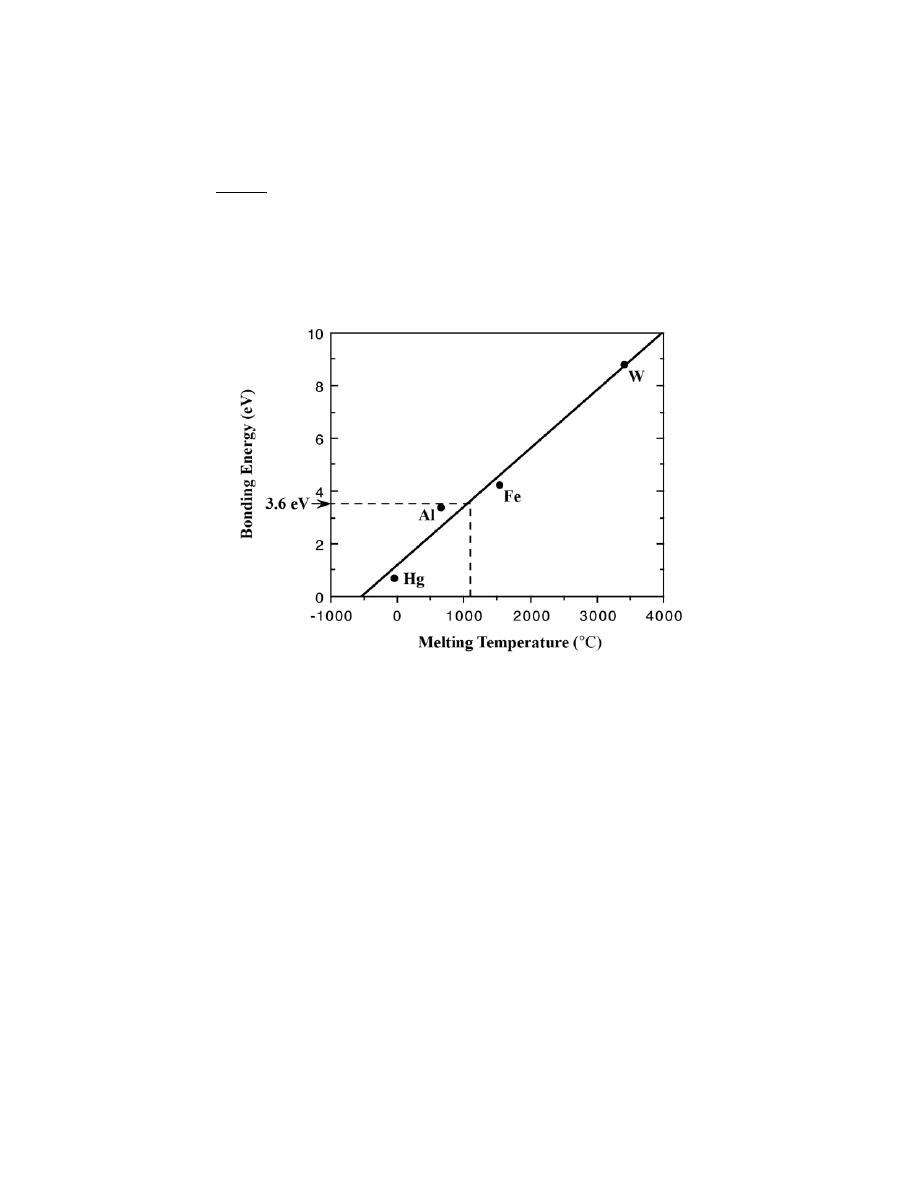
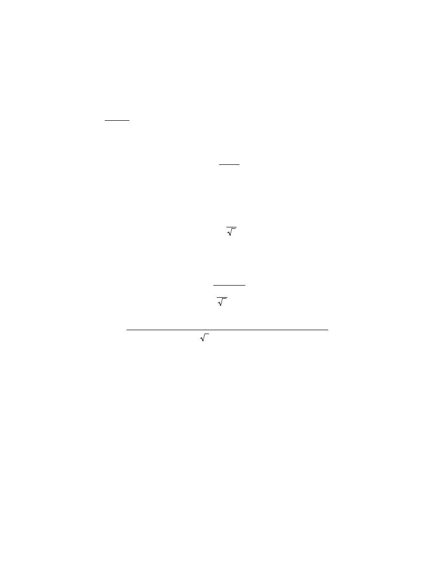
3.3 Show for the body-centered cubic crystal structure that the unit cell edge length a and the atomic
radius R are related through a =4R/
3
.
Solution
Consider the BCC unit cell shown below
Using the triangle NOP
(NP)
2
= a
2
+ a
2
= 2a
2
And then for triangle NPQ,
(NQ)
2 = (
QP)
2 + (
NP)
2
But
NQ
= 4R, R being the atomic radius. Also,
QP
= a. Therefore,
(4R)
2
= a
2
+ 2a
2
or
a =
4R
3
Excerpts from this work may be reproduced by instructors for distribution on a not-for-profit basis for testing or instructional purposes only to
students enrolled in courses for which the textbook has been adopted. Any other reproduction or translation of this work beyond that permitted
by Sections 107 or 108 of the 1976 United States Copyright Act without the permission of the copyright owner is unlawful.
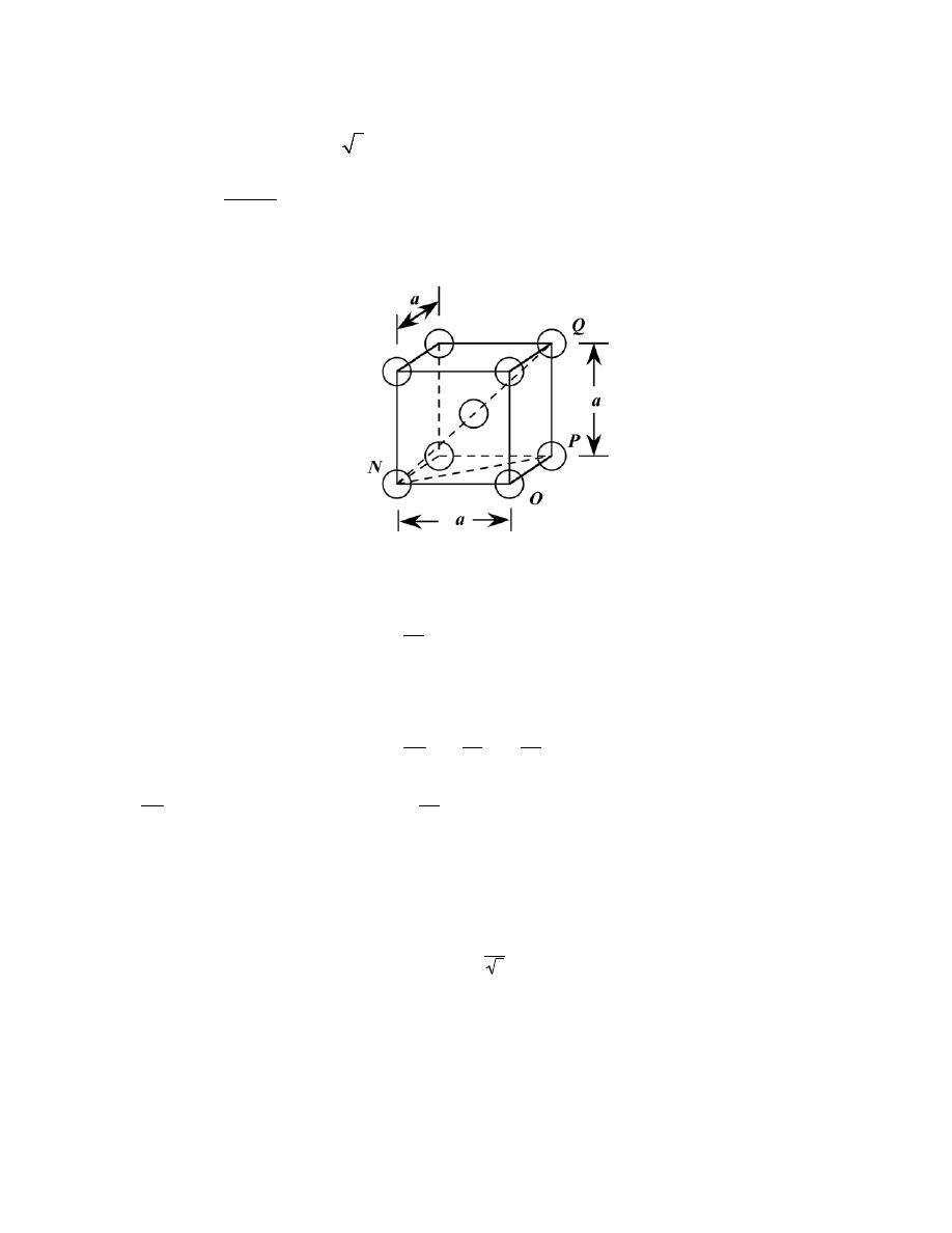
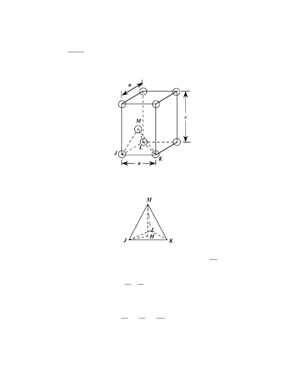
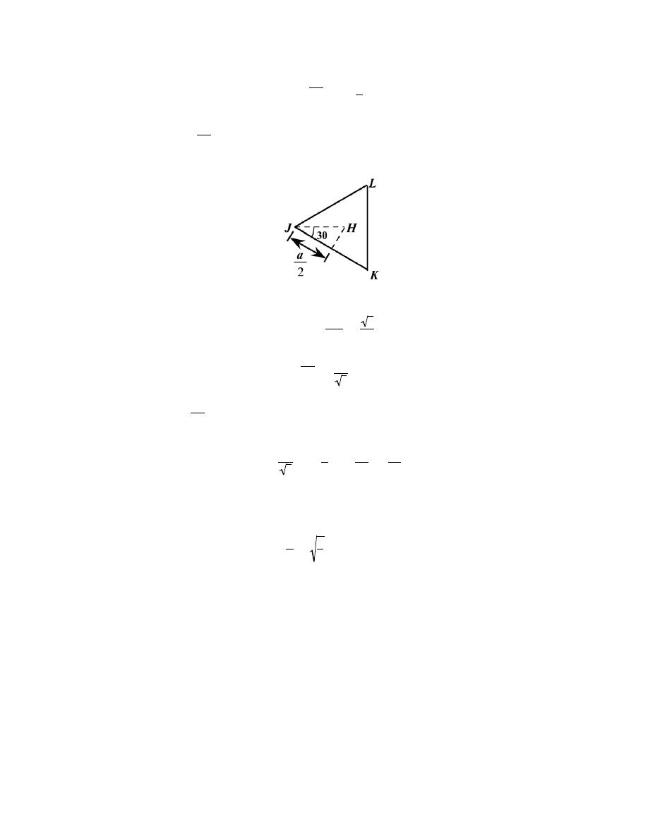
3.4 For the HCP crystal structure, show that the ideal c/a ratio is 1.633.
Solution
A sketch of one-third of an HCP unit cell is shown below.
Consider the tetrahedron labeled as JKLM, which is reconstructed as
The atom at point M is midway between the top and bottom faces of the unit cell--that is
MH = c/2. And, since
atoms at points J, K, and M, all touch one another,
JM = JK = 2R = a
where R is the atomic radius. Furthermore, from triangle JHM,
(JM )
2 = (
JH )
2 + (
MH )
2
or
Excerpts from this work may be reproduced by instructors for distribution on a not-for-profit basis for testing or instructional purposes only to
students enrolled in courses for which the textbook has been adopted. Any other reproduction or translation of this work beyond that permitted
by Sections 107 or 108 of the 1976 United States Copyright Act without the permission of the copyright owner is unlawful.
a
2
= ( JH )
2
+
c
2
2
Now, we can determine the
JH
length by consideration of triangle JKL, which is an equilateral triangle,
cos 30
° =
a /2
JH
=
3
2
and
JH =
a
3
Substituting this value for
JH in the above expression yields
a
2
=
a
3
2
+
c
2
2
=
a
2
3
+
c
2
4
and, solving for c/a
c
a
=
8
3
= 1.633
Excerpts from this work may be reproduced by instructors for distribution on a not-for-profit basis for testing or instructional purposes only to
students enrolled in courses for which the textbook has been adopted. Any other reproduction or translation of this work beyond that permitted
by Sections 107 or 108 of the 1976 United States Copyright Act without the permission of the copyright owner is unlawful.
3.5 Show that the atomic packing factor for BCC is 0.68.
Solution
The atomic packing factor is defined as the ratio of sphere volume to the total unit cell volume, or
APF =
V
S
V
C
Since there are two spheres associated with each unit cell for BCC
V
S
= 2 (sphere volume) = 2
4
πR
3
3
=
8
πR
3
3
Also, the unit cell has cubic symmetry, that is V
C
= a
3
. But a depends on R according to Equation 3.3, and
V
C
=
4R
3
3
=
64 R
3
3 3
Thus,
APF =
V
S
V
C
=
8
π R
3
/3
64 R
3
/3 3
= 0.68
Excerpts from this work may be reproduced by instructors for distribution on a not-for-profit basis for testing or instructional purposes only to
students enrolled in courses for which the textbook has been adopted. Any other reproduction or translation of this work beyond that permitted
by Sections 107 or 108 of the 1976 United States Copyright Act without the permission of the copyright owner is unlawful.
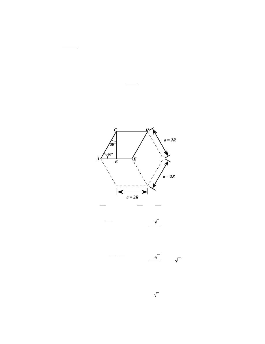
3.6 Show that the atomic packing factor for HCP is 0.74.
Solution
The APF is just the total sphere volume-unit cell volume ratio. For HCP, there are the equivalent of six
spheres per unit cell, and thus
V
S
= 6
4
π R
3
3
= 8π R
3
Now, the unit cell volume is just the product of the base area times the cell height, c. This base area is just three
times the area of the parallelepiped ACDE shown below.
The area of ACDE is just the length of
CD times the height
BC . But
CD is just a or 2R, and
BC = 2R cos (30
°) =
2 R 3
2
Thus, the base area is just
AREA = (3)(CD)(BC) = (3)(2 R)
2 R 3
2
= 6R
2
3
and since c = 1.633a = 2R(1.633)
V
C
= (AREA)(c) = 6 R
2
c 3
(3.S1)

Excerpts from this work may be reproduced by instructors for distribution on a not-for-profit basis for testing or instructional purposes only to
students enrolled in courses for which the textbook has been adopted. Any other reproduction or translation of this work beyond that permitted
by Sections 107 or 108 of the 1976 United States Copyright Act without the permission of the copyright owner is unlawful.
=
(
6 R
2
3
)
(2)(1.633)R = 12 3 (1.633) R
3
Thus,
APF =
V
S
V
C
=
8
π R
3
12 3 (1.633) R
3
= 0.74
Excerpts from this work may be reproduced by instructors for distribution on a not-for-profit basis for testing or instructional purposes only to
students enrolled in courses for which the textbook has been adopted. Any other reproduction or translation of this work beyond that permitted
by Sections 107 or 108 of the 1976 United States Copyright Act without the permission of the copyright owner is unlawful.
Density Computations
3.7 Iron has a BCC crystal structure, an atomic radius of 0.124 nm, and an atomic weight of 55.85 g/mol.
Compute and compare its theoretical density with the experimental value found inside the front cover.
Solution
This problem calls for a computation of the density of iron. According to Equation 3.5
ρ =
nA
Fe
V
C
N
A
For BCC, n = 2 atoms/unit cell, and
V
C
=
4 R
3
3
Thus,
ρ =
nA
Fe
4 R
3
3
N
A
=
(2 atoms/unit cell)(55.85 g/mol)
(4)
(
0.124
× 10
-7
cm
)
/ 3
[
]
3
/(unit cell)
(
6.022
× 10
23
atoms/mol
)
= 7.90 g/cm
3
The value given inside the front cover is 7.87 g/cm
3
.
Excerpts from this work may be reproduced by instructors for distribution on a not-for-profit basis for testing or instructional purposes only to
students enrolled in courses for which the textbook has been adopted. Any other reproduction or translation of this work beyond that permitted
by Sections 107 or 108 of the 1976 United States Copyright Act without the permission of the copyright owner is unlawful.
3.8 Calculate the radius of an iridium atom, given that Ir has an FCC crystal structure, a density of 22.4
g/cm
3
, and an atomic weight of 192.2 g/mol.
Solution
We are asked to determine the radius of an iridium atom, given that Ir has an FCC crystal structure. For
FCC, n = 4 atoms/unit cell, and V
C
=
16R
3
2 (Equation 3.4). Now,
ρ =
nA
Ir
V
C
N
A
=
nA
Ir
(
16R
3
2
)
N
A
And solving for R from the above expression yields
R =
nA
Ir
16
ρN
A
2
1/3
=
(4 atoms/unit cell) 192.2 g/mol
(
)
(16)
(
22.4 g/cm
3
)
(
6.022
× 10
23
atoms/mol
)
(
2
)
1/3
= 1.36
× 10
-8
cm = 0.136 nm
Excerpts from this work may be reproduced by instructors for distribution on a not-for-profit basis for testing or instructional purposes only to
students enrolled in courses for which the textbook has been adopted. Any other reproduction or translation of this work beyond that permitted
by Sections 107 or 108 of the 1976 United States Copyright Act without the permission of the copyright owner is unlawful.
3.9 Calculate the radius of a vanadium atom, given that V has a BCC crystal structure, a density of 5.96
g/cm
3
, and an atomic weight of 50.9 g/mol.
Solution
This problem asks for us to calculate the radius of a vanadium atom. For BCC, n = 2 atoms/unit cell, and
V
C
=
4 R
3
3
=
64 R
3
3 3
Since, from Equation 3.5
ρ =
nA
V
V
C
N
A
=
nA
V
64 R
3
3 3
N
A
and solving for R the previous equation
R =
3 3nA
V
64
ρ N
A
1/3
and incorporating values of parameters given in the problem statement
R =
(
3 3
)
(2 atoms/unit cell) (50.9 g/mol)
(64)
(
5.96 g/cm
3
)(
6.022
× 10
23
atoms/mol
)
1/3
= 1.32
× 10
-8
cm = 0.132 nm

Excerpts from this work may be reproduced by instructors for distribution on a not-for-profit basis for testing or instructional purposes only to
students enrolled in courses for which the textbook has been adopted. Any other reproduction or translation of this work beyond that permitted
by Sections 107 or 108 of the 1976 United States Copyright Act without the permission of the copyright owner is unlawful.
3.10 Some hypothetical metal has the simple cubic crystal structure shown in Figure 3.24. If its atomic
weight is 70.4 g/mol and the atomic radius is 0.126 nm, compute its density.
Solution
For the simple cubic crystal structure, the value of n in Equation 3.5 is unity since there is only a single
atom associated with each unit cell. Furthermore, for the unit cell edge length, a = 2R (Figure 3.24). Therefore,
employment of Equation 3.5 yields
ρ =
nA
V
C
N
A
=
nA
(2 R)
3
N
A
and incorporating values of the other parameters provided in the problem statement leads to
ρ =
(1 atom/unit cell)(70.4 g/mol)
(2)
(
1.26
× 10
-8
cm
)
3
/(unit cell)
(
6.022
× 10
23
atoms/mol
)
7.31 g/cm
3
Excerpts from this work may be reproduced by instructors for distribution on a not-for-profit basis for testing or instructional purposes only to
students enrolled in courses for which the textbook has been adopted. Any other reproduction or translation of this work beyond that permitted
by Sections 107 or 108 of the 1976 United States Copyright Act without the permission of the copyright owner is unlawful.
3.11 Zirconium has an HCP crystal structure and a density of 6.51 g/cm
3
.
(a) What is the volume of its unit cell in cubic meters?
(b) If the c/a ratio is 1.593, compute the values of c and a.
Solution
(a) The volume of the Zr unit cell may be computed using Equation 3.5 as
V
C
=
nA
Zr
ρN
A
Now, for HCP, n = 6 atoms/unit cell, and for Zr, A
Zr
= 91.22 g/mol. Thus,
V
C
=
(6 atoms/unit cell)(91.22 g/mol)
(
6.51 g/cm
3
)(
6.022
× 10
23
atoms/mol
)
= 1.396
× 10
-22
cm
3
/unit cell = 1.396
× 10
-28
m
3
/unit cell
(b) From Equation 3.S1 of the solution to Problem 3.6, for HCP
V
C
= 6 R
2
c 3
But, since a = 2R, (i.e., R = a/2) then
V
C
= 6
a
2
2
c 3
=
3 3 a
2
c
2
but, since c = 1.593a
V
C
=
3 3 (1.593) a
3
2
= 1.396
× 10
-22
cm
3
/unit cell
Now, solving for a
a =
(2)
(
1.396
× 10
-22
cm
3
)
(3)
(
3
)
(1.593)
1/3

Excerpts from this work may be reproduced by instructors for distribution on a not-for-profit basis for testing or instructional purposes only to
students enrolled in courses for which the textbook has been adopted. Any other reproduction or translation of this work beyond that permitted
by Sections 107 or 108 of the 1976 United States Copyright Act without the permission of the copyright owner is unlawful.
= 3.23
× 10
-8
cm = 0.323 nm
And finally
c = 1.593a = (1.593)(0.323 nm) = 0.515 nm
Excerpts from this work may be reproduced by instructors for distribution on a not-for-profit basis for testing or instructional purposes only to
students enrolled in courses for which the textbook has been adopted. Any other reproduction or translation of this work beyond that permitted
by Sections 107 or 108 of the 1976 United States Copyright Act without the permission of the copyright owner is unlawful.
3.12 Using atomic weight, crystal structure, and atomic radius data tabulated inside the front cover,
compute the theoretical densities of lead, chromium, copper, and cobalt, and then compare these values with the
measured densities listed in this same table. The c/a ratio for cobalt is 1.623.
Solution
Since Pb has an FCC crystal structure, n = 4, and V
C
=
16R
3
2 (Equation 3.4). Also, R = 0.175 nm (1.75
× 10
-8
cm) and A
Pb
= 207.2 g/mol. Employment of Equation 3.5 yields
ρ =
nA
Pb
V
C
N
A
=
(4 atoms/unit cell)(207.2 g/mol)
(16)
(
1.75
× 10
-8
cm
)
3
(
2
)
[
]
/(unit cell)
{
}
(
6.022
× 10
23
atoms/mol
)
= 11.35 g/cm3
The value given in the table inside the front cover is 11.35 g/cm3.
Chromium has a BCC crystal structure for which n = 2 and V
C
= a
3
=
4 R
3
3
(Equation 3.3); also A
Cr
=
52.00g/mol and R = 0.125 nm. Therefore, employment of Equation 3.5 leads to
ρ =
(2 atoms/unit cell)(52.00 g/mol)
(4)
(
1.25
× 10
-8
cm
)
3
3
/(unit cell)
(
6.022
× 1023 atoms/mol
)
= 7.18 g/cm3
The value given in the table is 7.19 g/cm3.
Copper also has an FCC crystal structure and therefore
ρ =
(4 atoms/unit cell)(63.55 g/mol)
(2)
(
1.28
× 10
-8
cm
)(
2
)
[
]
3
/(unit cell)
(
6.022
× 10
23
atoms/mol
)
= 8.90 g/cm
3

Excerpts from this work may be reproduced by instructors for distribution on a not-for-profit basis for testing or instructional purposes only to
students enrolled in courses for which the textbook has been adopted. Any other reproduction or translation of this work beyond that permitted
by Sections 107 or 108 of the 1976 United States Copyright Act without the permission of the copyright owner is unlawful.
The value given in the table is 8.90 g/cm
3
.
Cobalt has an HCP crystal structure, and from the solution to Problem 3.6 (Equation 3.S1),
V
C
= 6R
2
c 3
and, since c = 1.623a and a = 2R, c = (1.623)(2R); hence
V
C
= 6R
2
(1.623)(2R) 3
= (19.48)( 3)R
3
= (19.48)( 3)(1.25 × 10
−8
cm)
3
= 6.59 × 10
−23
cm
3
/unit cell
Also, there are 6 atoms/unit cell for HCP. Therefore the theoretical density is
ρ =
nA
Co
V
C
N
A
=
(6 atoms/unit cell)(58.93 g/mol)
(
6.59
× 10
-23
cm
3
/unit cell
)(
6.022
× 10
23
atoms/mol
)
= 8.91 g/cm
3
The value given in the table is 8.9 g/cm
3
.
Excerpts from this work may be reproduced by instructors for distribution on a not-for-profit basis for testing or instructional purposes only to
students enrolled in courses for which the textbook has been adopted. Any other reproduction or translation of this work beyond that permitted
by Sections 107 or 108 of the 1976 United States Copyright Act without the permission of the copyright owner is unlawful.
3.13 Rhodium has an atomic radius of 0.1345 nm and a density of 12.41 g/cm
3
. Determine whether it has
an FCC or BCC crystal structure.
Solution
In order to determine whether Rh has an FCC or a BCC crystal structure, we need to compute its density
for each of the crystal structures. For FCC, n = 4, and a =
2 R 2
(Equation 3.1). Also, from Figure 2.6, its atomic
weight is 102.91 g/mol. Thus, for FCC (employing Equation 3.5)
ρ =
nA
Rh
a3N A
=
nA
Rh
(
2R 2
)
3 N
A
=
(4 atoms/unit cell)(102.91 g/mol)
(2)
(
1.345
× 10
-8
cm
)
(
2
)
[
]
3
/(unit cell)
(
6.022
× 10
23
atoms / mol
)
= 12.41 g/cm
3
which is the value provided in the problem statement. Therefore, Rh has the FCC crystal structure.

Excerpts from this work may be reproduced by instructors for distribution on a not-for-profit basis for testing or instructional purposes only to
students enrolled in courses for which the textbook has been adopted. Any other reproduction or translation of this work beyond that permitted
by Sections 107 or 108 of the 1976 United States Copyright Act without the permission of the copyright owner is unlawful.
3.14 Below are listed the atomic weight, density, and atomic radius for three hypothetical alloys. For
each determine whether its crystal structure is FCC, BCC, or simple cubic and then justify your determination. A
simple cubic unit cell is shown in Figure 3.24.
Alloy
Atomic Weight
Density
Atomic Radius
(g/mol)
(g/cm
3
)
(nm)
A
77.4
8.22
0.125
B
107.6
13.42
0.133
C
127.3
9.23
0.142
Solution
For each of these three alloys we need, by trial and error, to calculate the density using Equation 3.5, and
compare it to the value cited in the problem. For SC, BCC, and FCC crystal structures, the respective values of n
are 1, 2, and 4, whereas the expressions for a (since V
C
= a
3
) are 2R,
2 R 2
, and
4R
3
.
For alloy A, let us calculate
ρ assuming a simple cubic crystal structure.
ρ =
nA
A
V
C
N
A
=
nA
A
2R
( )
3
N
A
=
(1 atom/unit cell)(77.4 g/mol)
(2)(1.25
× 10
−8
)
[
]
3
/(unit cell)
(
6.022
× 10
23
atoms/mol
)
= 8.22 g/cm3
Therefore, its crystal structure is simple cubic.
For alloy B, let us calculate
ρ assuming an FCC crystal structure.
ρ =
nA
B
(2 R 2)
3
N
A
Excerpts from this work may be reproduced by instructors for distribution on a not-for-profit basis for testing or instructional purposes only to
students enrolled in courses for which the textbook has been adopted. Any other reproduction or translation of this work beyond that permitted
by Sections 107 or 108 of the 1976 United States Copyright Act without the permission of the copyright owner is unlawful.
=
(4 atoms/unit cell)(107.6 g/mol)
2 2
( )
(
1.33
× 10
-8
cm
)
[
]
3
/(unit cell)
(
6.022
× 10
23
atoms/mol
)
= 13.42 g/cm
3
Therefore, its crystal structure is FCC.
For alloy C, let us calculate
ρ assuming a simple cubic crystal structure.
=
nA
C
2R
( )
3
N
A
=
(1 atom/unit cell)(127.3 g/mol)
(2)
(
1.42
× 10
-8
cm
)
[
]
3
/(unit cell)
(
6.022
× 10
23
atoms/mol
)
= 9.23 g/cm
3
Therefore, its crystal structure is simple cubic.
Excerpts from this work may be reproduced by instructors for distribution on a not-for-profit basis for testing or instructional purposes only to
students enrolled in courses for which the textbook has been adopted. Any other reproduction or translation of this work beyond that permitted
by Sections 107 or 108 of the 1976 United States Copyright Act without the permission of the copyright owner is unlawful.
3.15 The unit cell for tin has tetragonal symmetry, with a and b lattice parameters of 0.583 and 0.318 nm,
respectively. If its density, atomic weight, and atomic radius are 7.30 g/cm
3
, 118.69 g/mol, and 0.151 nm,
respectively, compute the atomic packing factor.
Solution
In order to determine the APF for Sn, we need to compute both the unit cell volume (V
C
) which is just the
a
2
c product, as well as the total sphere volume (V
S
) which is just the product of the volume of a single sphere and
the number of spheres in the unit cell (n). The value of n may be calculated from Equation 3.5 as
n =
ρV
C
N
A
A
Sn
=
(7.30 g/cm
3
)(5.83)
2
(3.18)
(
× 10
-24
cm
3
)(
6.022
× 10
23
atoms / mol
)
118.69 g/mol
= 4.00 atoms/unit cell
Therefore
APF =
V
S
V
C
=
(4)
4
3
π R
3
(a)
2
(c)
=
(4)
4
3
(
π)(1.51 × 10
-8
cm)
3
(5.83
× 10
-8
cm)
2
(3.18
× 10
-8
cm)
= 0.534
Excerpts from this work may be reproduced by instructors for distribution on a not-for-profit basis for testing or instructional purposes only to
students enrolled in courses for which the textbook has been adopted. Any other reproduction or translation of this work beyond that permitted
by Sections 107 or 108 of the 1976 United States Copyright Act without the permission of the copyright owner is unlawful.
3.16 Iodine has an orthorhombic unit cell for which the a, b, and c lattice parameters are 0.479, 0.725,
and 0.978 nm, respectively.
(a) If the atomic packing factor and atomic radius are 0.547 and 0.177 nm, respectively, determine the
number of atoms in each unit cell.
(b) The atomic weight of iodine is 126.91 g/mol; compute its theoretical density.
Solution
(a) For indium, and from the definition of the APF
APF =
V
S
V
C
=
n
4
3
π R
3
abc
we may solve for the number of atoms per unit cell, n, as
n =
(APF) abc
4
3
π R
3
Incorporating values of the above parameters provided in the problem state leads to
=
(0.547)(4.79
× 10
-8
cm)(7.25
× 10
-8
cm)
(
9.78
× 10
-8
cm
)
4
3
π
(
1.77
× 10
-8
cm
)
3
= 8.0 atoms/unit cell
(b) In order to compute the density, we just employ Equation 3.5 as
ρ =
nA
I
abc N
A
=
(8 atoms/unit cell)(126.91 g/mol)
(4.79
× 10
-8
cm)(7.25
× 10
-8
cm)
(
9.78
× 10
-8
cm
)
[
]
/ unit cell
{
}
(
6.022
× 10
23
atoms/mol
)
= 4.96 g/cm
3
Excerpts from this work may be reproduced by instructors for distribution on a not-for-profit basis for testing or instructional purposes only to
students enrolled in courses for which the textbook has been adopted. Any other reproduction or translation of this work beyond that permitted
by Sections 107 or 108 of the 1976 United States Copyright Act without the permission of the copyright owner is unlawful.
3. 17 Titanium has an HCP unit cell for which the ratio of the lattice parameters c/a is 1.58. If the radius
of the Ti atom is 0.1445 nm, (a) determine the unit cell volume, and (b) calculate the density of Ti and compare it
with the literature value.
Solution
(a) We are asked to calculate the unit cell volume for Ti. For HCP, from Equation 3.S1 (found in the
solution to Problem 3.6)
V
C
= 6 R
2
c 3
But for Ti, c = 1.58a, and a = 2R, or c = 3.16R, and
V
C
= (6)(3.16) R
3
3
= (6) (3.16)
(
3
)
1.445
× 10
-8
cm
[
]
3
= 9.91
× 10
−23
cm
3
/unit cell
(b) The theoretical density of Ti is determined, using Equation 3.5, as follows:
ρ =
nA
Ti
V
C
N
A
For HCP, n = 6 atoms/unit cell, and for Ti, A
Ti
= 47.87 g/mol (as noted inside the front cover). Thus,
ρ =
(6 atoms/unit cell)(47.87 g/mol)
(
9.91
× 10
-23
cm
3
/unit cell
)(
6.022
× 10
23
atoms/mol
)
= 4.81 g/cm
3
The value given in the literature is 4.51 g/cm
3
.
Excerpts from this work may be reproduced by instructors for distribution on a not-for-profit basis for testing or instructional purposes only to
students enrolled in courses for which the textbook has been adopted. Any other reproduction or translation of this work beyond that permitted
by Sections 107 or 108 of the 1976 United States Copyright Act without the permission of the copyright owner is unlawful.
3.18 Zinc has an HCP crystal structure, a c/a ratio of 1.856, and a density of 7.13 g/cm
3
. Compute the
atomic radius for Zn.
Solution
In order to calculate the atomic radius for Zn, we must use Equation 3.5, as well as the expression which
relates the atomic radius to the unit cell volume for HCP; Equation 3.S1 (from Problem 3.6) is as follows:
V
C
= 6 R
2
c 3
In this case c = 1.856a, but, for HCP, a = 2R, which means that
V
C
= 6 R
2
(1.856)(2R) 3
= (1.856)
(
12 3
)
R
3
And from Equation 3.5, the density is equal to
ρ =
nA
Zn
V
C
N
A
=
nA
Zn
(1.856)
(
12 3
)
R
3
N
A
And, solving for R from the above equation leads to the following:
R =
nA
Zn
(1.856)
(
12
3
)
ρ N
A
1/3
And incorporating appropriate values for the parameters in this equation leads to
R =
(6 atoms/unit cell) (65.41 g/mol)
(1.856)
(
12
3
)(
7.13 g/cm
3
)(
6.022
× 10
23
atoms/mol
)
1/3
= 1.33
× 10
-8
cm = 0.133 nm

Excerpts from this work may be reproduced by instructors for distribution on a not-for-profit basis for testing or instructional purposes only to
students enrolled in courses for which the textbook has been adopted. Any other reproduction or translation of this work beyond that permitted
by Sections 107 or 108 of the 1976 United States Copyright Act without the permission of the copyright owner is unlawful.
3.19 Rhenium has an HCP crystal structure, an atomic radius of 0.137 nm, and a c/a ratio of 1.615.
Compute the volume of the unit cell for Re.
Solution
In order to compute the volume of the unit cell for Re, it is necessary to use Equation 3.S1 (found in Problem 3.6),
that is
V
C
= 6 R
2
c 3
The problem states that c = 1.615a, and a = 2R. Therefore
V
C
= (1.615)
(
12 3
)
R
3
= (1.615)
(
12 3
)
(
1.37
× 10
-8
cm
)
3
= 8.63
× 10
-23
cm
3
= 8.63
× 10
-2
nm
3
Excerpts from this work may be reproduced by instructors for distribution on a not-for-profit basis for testing or instructional purposes only to
students enrolled in courses for which the textbook has been adopted. Any other reproduction or translation of this work beyond that permitted
by Sections 107 or 108 of the 1976 United States Copyright Act without the permission of the copyright owner is unlawful.
Crystal Systems
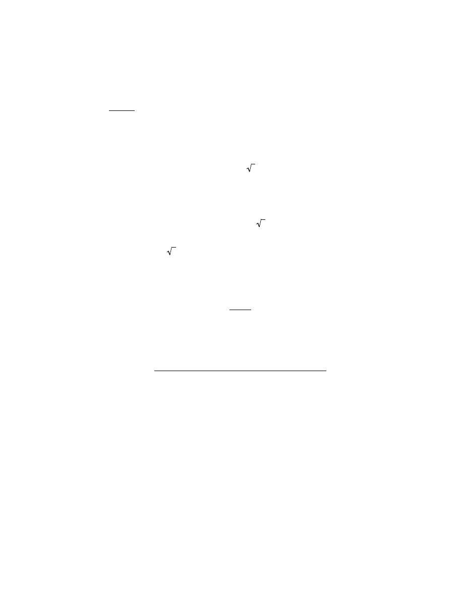
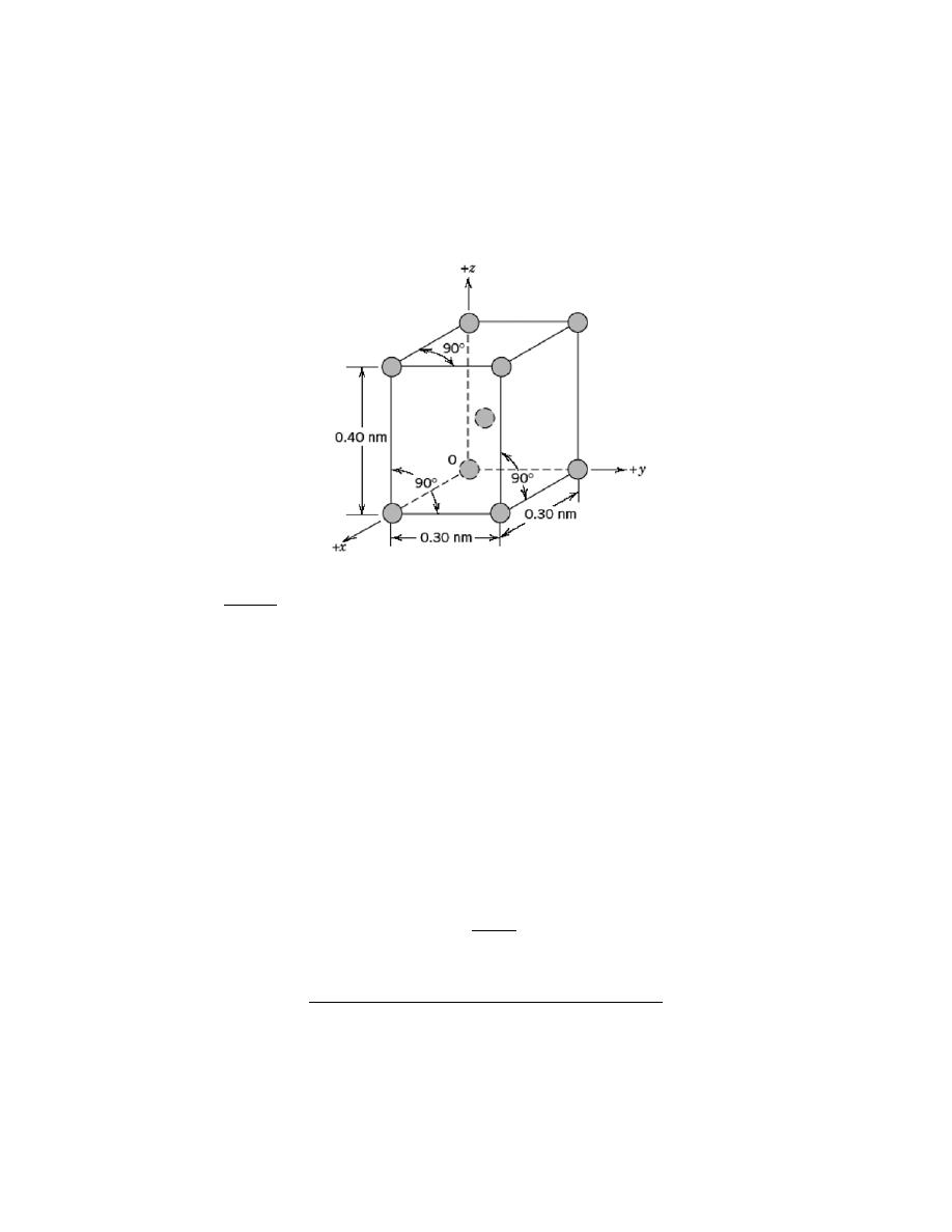
3.20 Below is a unit cell for a hypothetical metal.
(a) To which crystal system does this unit cell belong?
(b) What would this crystal structure be called?
(c) Calculate the density of the material, given that its atomic weight is 141 g/mol.
Solution
(a) The unit cell shown in the problem statement belongs to the tetragonal crystal system since a = b =
0.30 nm, c = 0.40 nm, and
α = β = γ = 90°.
(b) The crystal structure would be called body-centered tetragonal.
(c) As with BCC, n = 2 atoms/unit cell. Also, for this unit cell
V
C
=
(
3.0
× 10
−8
cm
)
2
(
4.0
× 10
−8
cm
)
= 3.60
× 10
−23
cm
3
/unit cell
Thus, using Equation 3.5, the density is equal to
ρ =
nA
V
C
N
A
=
(2 atoms/unit cell) (141 g/mol)
(
3.60
× 10
-23
cm
3
/unit cell
)(
6.022
× 10
23
atoms/mol
)
= 13.0 g/cm
3
Excerpts from this work may be reproduced by instructors for distribution on a not-for-profit basis for testing or instructional purposes only to
students enrolled in courses for which the textbook has been adopted. Any other reproduction or translation of this work beyond that permitted
by Sections 107 or 108 of the 1976 United States Copyright Act without the permission of the copyright owner is unlawful.
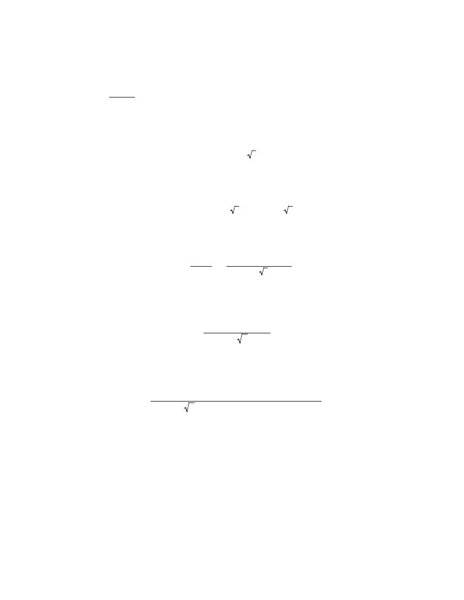
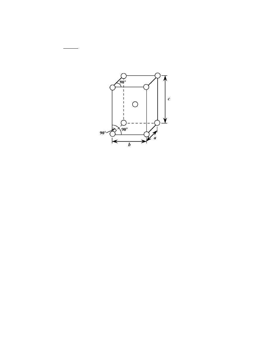
3.21 Sketch a unit cell for the body-centered orthorhombic crystal structure.
Solution
A unit cell for the body-centered orthorhombic crystal structure is presented below.

Excerpts from this work may be reproduced by instructors for distribution on a not-for-profit basis for testing or instructional purposes only to
students enrolled in courses for which the textbook has been adopted. Any other reproduction or translation of this work beyond that permitted
by Sections 107 or 108 of the 1976 United States Copyright Act without the permission of the copyright owner is unlawful.
Point Coordinates
3.22 List the point coordinates for all atoms that are associated with the FCC unit cell (Figure 3.1).
Solution
From Figure 3.1b, the atom located of the origin of the unit cell has the coordinates 000. Coordinates for
other atoms in the bottom face are 100, 110, 010, and
1
2
1
2
0. (The z coordinate for all these points is zero.)
For the top unit cell face, the coordinates are 001, 101, 111, 011, and
1
2
1
2
1.
Coordinates for those atoms that are positioned at the centers of both side faces, and centers of both front
and back faces need to be specified. For the front and back-center face atoms, the coordinates are
1
1
2
1
2
and
0
1
2
1
2
,
respectively. While for the left and right side center-face atoms, the respective coordinates are
1
2
0
1
2
and
1
2
1
1
2
.
Excerpts from this work may be reproduced by instructors for distribution on a not-for-profit basis for testing or instructional purposes only to
students enrolled in courses for which the textbook has been adopted. Any other reproduction or translation of this work beyond that permitted
by Sections 107 or 108 of the 1976 United States Copyright Act without the permission of the copyright owner is unlawful.
3.23 List the point coordinates of the titanium, barium, and oxygen ions for a unit cell of the perovskite
crystal structure (Figure 12.6).
Solution
In Figure 12.6, the barium ions are situated at all corner positions. The point coordinates for these ions are
as follows: 000, 100, 110, 010, 001, 101, 111, and 011.
The oxygen ions are located at all face-centered positions; therefore, their coordinates are
1
2
1
2
0,
1
2
1
2
1,
1
1
2
1
2
,
0
1
2
1
2
,
1
2
0
1
2
, and
1
2
1
1
2
.
And, finally, the titanium ion resides at the center of the cubic unit cell, with coordinates
1
2
1
2
1
2
.
Excerpts from this work may be reproduced by instructors for distribution on a not-for-profit basis for testing or instructional purposes only to
students enrolled in courses for which the textbook has been adopted. Any other reproduction or translation of this work beyond that permitted
by Sections 107 or 108 of the 1976 United States Copyright Act without the permission of the copyright owner is unlawful.
3.24 List the point coordinates of all atoms that are associated with the diamond cubic unit cell (Figure
12.15).
Solution
First of all, one set of carbon atoms occupy all corner positions of the cubic unit cell; the coordinates of
these atoms are as follows: 000, 100, 110, 010, 001, 101, 111, and 011.
Another set of atoms reside on all of the face-centered positions, with the following coordinates:
1
2
1
2
0,
1
2
1
2
1,
1
1
2
1
2
,
0
1
2
1
2
,
1
2
0
1
2
, and
1
2
1
1
2
.
The third set of carbon atoms are positioned within the interior of the unit cell. Using an x-y-z coordinate
system oriented as in Figure 3.4, the coordinates of the atom that lies toward the lower-left-front of the unit cell has
the coordinates
3
4
1
4
1
4
, whereas the atom situated toward the lower-right-back of the unit cell has coordinates of
1
4
3
4
1
4
. Also, the carbon atom that resides toward the upper-left-back of the unit cell has the
1
4
1
4
3
4
coordinates.
And, the coordinates of the final atom, located toward the upper-right-front of the unit cell, are
3
4
3
4
3
4
.
Excerpts from this work may be reproduced by instructors for distribution on a not-for-profit basis for testing or instructional purposes only to
students enrolled in courses for which the textbook has been adopted. Any other reproduction or translation of this work beyond that permitted
by Sections 107 or 108 of the 1976 United States Copyright Act without the permission of the copyright owner is unlawful.
3.25 Sketch a tetragonal unit cell , and within that cell indicate locations of the
1
2
1
1
2
and
1
4
1
2
3
4
point
coordinates.
Solution
A tetragonal unit in which are shown the
1
2
1
1
2
and
1
4
1
2
3
4
point coordinates is presented below.

Excerpts from this work may be reproduced by instructors for distribution on a not-for-profit basis for testing or instructional purposes only to
students enrolled in courses for which the textbook has been adopted. Any other reproduction or translation of this work beyond that permitted
by Sections 107 or 108 of the 1976 United States Copyright Act without the permission of the copyright owner is unlawful.
3.26 Using the Molecule Definition Utility found in both “Metallic Crystal Structures and
Crystallography” and “Ceramic Crystal Structures” modules of VMSE, located on the book’s web site
[www.wiley.com/college/Callister (Student Companion Site)], generate a three-dimensional unit cell for the
intermetallic compound AuCu
3
given the following: (1) the unit cell is cubic with an edge length of 0.374 nm, (2)
gold atoms are situated at all cube corners, and (3) copper atoms are positioned at the centers of all unit cell faces.
Solution
First of all, open the “Molecular Definition Utility”; it may be found in either of “Metallic Crystal
Structures and Crystallography” or “Ceramic Crystal Structures” modules.
In the “Step 1” window, it is necessary to define the atom types, colors for the spheres (atoms), and specify
atom sizes. Let us enter “Au” as the name for the gold atoms (since “Au” the symbol for gold), and “Cu” as the
name for the copper atoms. Next it is necessary to choose a color for each atom type from the selections that appear
in the pull-down menu—for example, “Yellow” for Au and “Red” for Cu. In the “Atom Size” window, it is
necessary to enter an atom/ion size. In the instructions for this step, it is suggested that the atom/ion diameter in
nanometers be used. From the table found inside the front cover of the textbook, the atomic radii for gold and
copper are 0.144 nm and 0.128 nm, respectively, and, therefore, their ionic diameters are twice these values (i.e.,
0.288 nm and 0.256 nm); therefore, we enter the values “0.288” and “0.256” for the two atom types. Now click on
the “Register” button, followed by clicking on the “Go to Step 2” button.
In the “Step 2” window we specify positions for all of the atoms within the unit cell; their point
coordinates are specified in the problem statement. Let’s begin with gold. Click on the yellow sphere that is
located to the right of the “Molecule Definition Utility” box. Again, Au atoms are situated at all eight corners of the
cubic unit cell. One Au will be positioned at the origin of the coordinate system—i.e., its point coordinates are 000,
and, therefore, we enter a “0” (zero) in each of the “x”, “y”, and “z” atom position boxes. Next we click on the
“Register Atom Position” button. Now we enter the coordinates of another gold atom; let us arbitrarily select the
one that resides at the corner of the unit cell that is one unit-cell length along the x-axis (i.e., at the 100 point
coordinate). Inasmuch as it is located a distance of a units along the x-axis the value of “0.374” is entered in the “x”
atom position box (since this is the value of a given in the problem statement); zeros are entered in each of the “y”
and “z” position boxes. We repeat this procedure for the remaining six Au atoms.
After this step has been completed, it is necessary to specify positions for the copper atoms, which are
located at all six face-centered sites. To begin, we click on the red sphere that is located next to the “Molecule
Definition Utility” box. The point coordinates for some of the Cu atoms are fractional ones; in these instances, the a
unit cell length (i.e., 0.374) is multiplied by the fraction. For example, one Cu atom is located
1
1
2
1
2
coordinate.
Therefore, the x, y, and z atoms positions are (1)(0.374) = 0.374,
1
2
(0.374) = 0.187, and
1
2
(0.374) = 0.187,
respectively.
For the gold atoms, the x, y, and z atom position entries for all 8 sets of point coordinates are as follows:
Excerpts from this work may be reproduced by instructors for distribution on a not-for-profit basis for testing or instructional purposes only to
students enrolled in courses for which the textbook has been adopted. Any other reproduction or translation of this work beyond that permitted
by Sections 107 or 108 of the 1976 United States Copyright Act without the permission of the copyright owner is unlawful.
0, 0, and 0
0.374, 0, and 0
0, 0.374, and 0
0, 0, and 0.374
0, 0.374, 0.374
0.374, 0, 0.374
0.374, 0.374, 0
0.374, 0.374, 0.374
Now, for the copper atoms, the x, y, and z atom position entries for all 6 sets of point coordinates are as
follows:
0.187, 0.187, 0
0.187, 0, 0.187
0, 0.187, 0.187
0.374, 0.187, 0.187
0.187, 0.374, 0.187
0.187, 0.187, 0.374
In Step 3, we may specify which atoms are to be represented as being bonded to one another, and which
type of bond(s) to use (single solid, single dashed, double, and triple are possibilities), or we may elect to not
represent any bonds at all (in which case we are finished). If it is decided to show bonds, probably the best thing to
do is to represent unit cell edges as bonds. This image may be rotated by using mouse click-and-drag
Your image should appear as the following screen shot. Here the gold atoms appear lighter than the copper
atoms.

Excerpts from this work may be reproduced by instructors for distribution on a not-for-profit basis for testing or instructional purposes only to
students enrolled in courses for which the textbook has been adopted. Any other reproduction or translation of this work beyond that permitted
by Sections 107 or 108 of the 1976 United States Copyright Act without the permission of the copyright owner is unlawful.
[Note: Unfortunately, with this version of the Molecular Definition Utility, it is not possible to save either the data
or the image that you have generated. You may use screen capture (or screen shot) software to record and store
your image.]
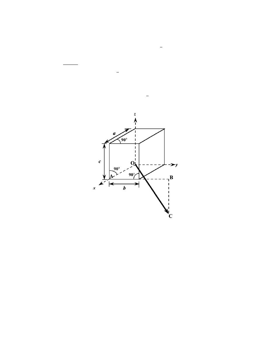
Excerpts from this work may be reproduced by instructors for distribution on a not-for-profit basis for testing or instructional purposes only to
students enrolled in courses for which the textbook has been adopted. Any other reproduction or translation of this work beyond that permitted
by Sections 107 or 108 of the 1976 United States Copyright Act without the permission of the copyright owner is unlawful.
Crystallographic Directions
3.27 Draw an orthorhombic unit cell, and within that cell a
[121 ]
direction.
Solution
This problem calls for us to draw a
[12 1 ] direction within an orthorhombic unit cell (a
≠ b ≠ c, α = β = γ =
90
°). Such a unit cell with its origin positioned at point O is shown below. We first move along the +x-axis a units
(from point O to point A), then parallel to the +y-axis 2b units (from point A to point B). Finally, we proceed
parallel to the z-axis -c units (from point B to point C). The
[12 1 ] direction is the vector from the origin (point O)
to point C as shown.
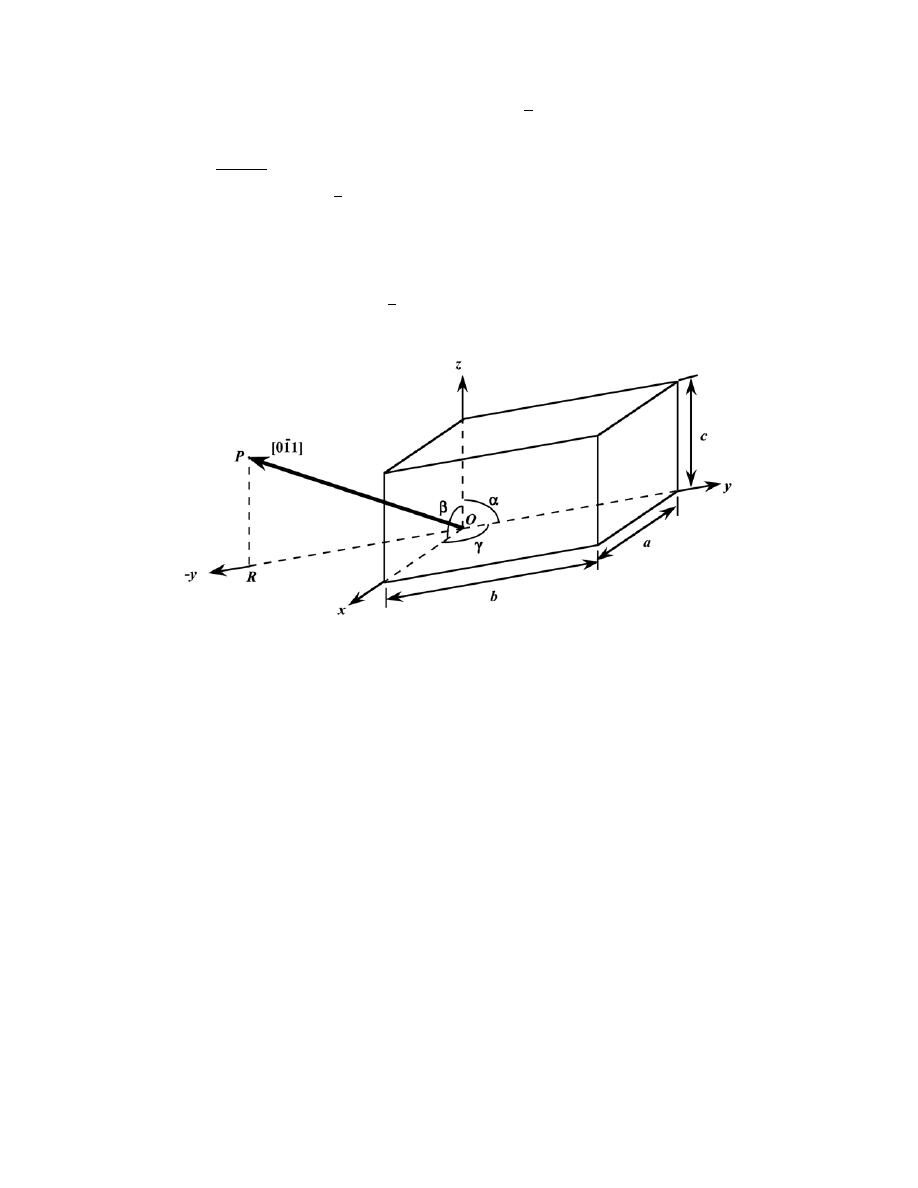
Excerpts from this work may be reproduced by instructors for distribution on a not-for-profit basis for testing or instructional purposes only to
students enrolled in courses for which the textbook has been adopted. Any other reproduction or translation of this work beyond that permitted
by Sections 107 or 108 of the 1976 United States Copyright Act without the permission of the copyright owner is unlawful.
3.28 Sketch a monoclinic unit cell, and within that cell a
[01 1 ] direction.
Solution
This problem asks that a
[ 0 1 1 ]
direction be drawn within a monoclinic unit cell (a
≠ b ≠ c, and α = β =
90º ≠ γ). One such unit cell with its origin at point O is sketched below. For this direction, there is no projection
along the x-axis since the first index is zero; thus, the direction lies in the y-z plane. We next move from the origin
along the minus y-axis b units (from point O to point R). Since the final index is a one, move from point R parallel
to the z-axis, c units (to point P). Thus, the
[ 0 1 1 ]
direction corresponds to the vector passing from the origin (point
O) to point P, as indicated in the figure.
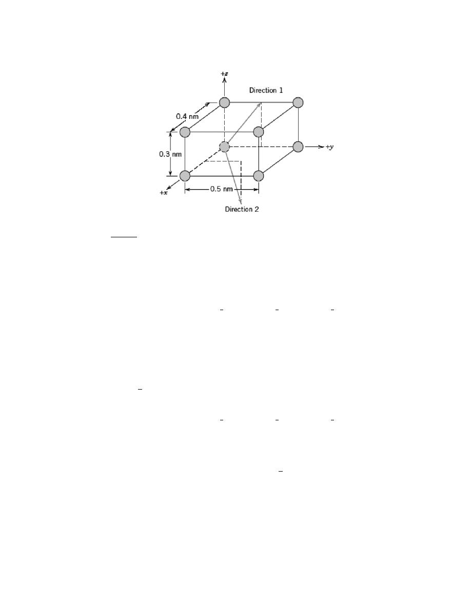
Excerpts from this work may be reproduced by instructors for distribution on a not-for-profit basis for testing or instructional purposes only to
students enrolled in courses for which the textbook has been adopted. Any other reproduction or translation of this work beyond that permitted
by Sections 107 or 108 of the 1976 United States Copyright Act without the permission of the copyright owner is unlawful.
3.29 What are the indices for the directions indicated by the two vectors in the sketch below?
Solution
For direction 1, the projection on the x-axis is zero (since it lies in the y-z plane), while projections on the
y- and z-axes, b/2 and c, respectively. This is a
[ 012 ] direction as indicated in the summary below.
x
y
z
Projections
0a
b/2
c
Projections in terms of a, b, and c
0
1/2
1
Reduction to integers
0
1
2
Enclosure
[ 012 ]
Direction 2 is
[112 ] as summarized below.
x
y
z
Projections
a/2
b/2
-c
Projections in terms of a, b, and c
1/2
1/2
-1
Reduction to integers
1
1
-2
Enclosure
[112 ]
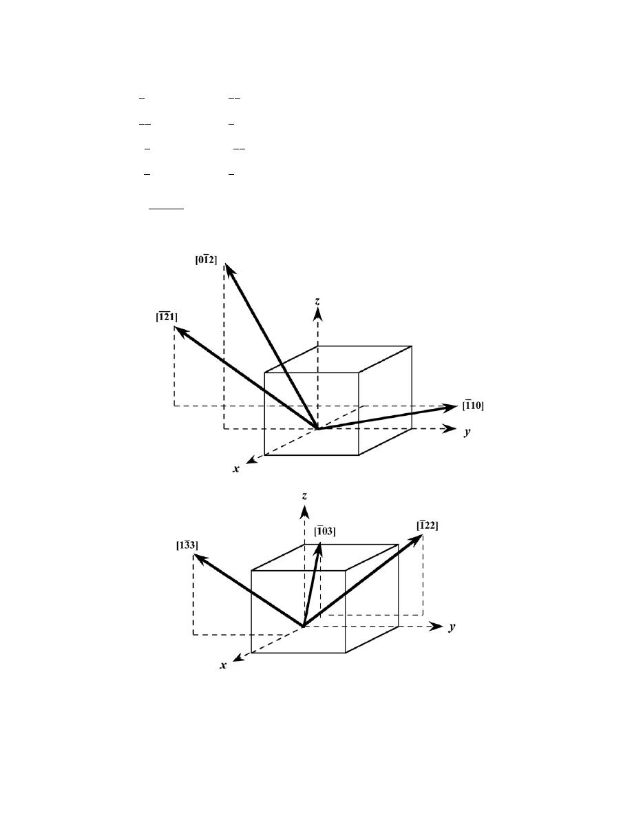
Excerpts from this work may be reproduced by instructors for distribution on a not-for-profit basis for testing or instructional purposes only to
students enrolled in courses for which the textbook has been adopted. Any other reproduction or translation of this work beyond that permitted
by Sections 107 or 108 of the 1976 United States Copyright Act without the permission of the copyright owner is unlawful.
3.30 Within a cubic unit cell, sketch the following directions:
(a)
[1 10],
(e)
[1 1 1] ,
(b)
[1 2 1],
(f)
[1 22],
(c)
[01 2],
(g)
[12 3 ],
(d)
[13 3],
(h)
[ 1 03].
Solution
The directions asked for are indicated in the cubic unit cells shown below.
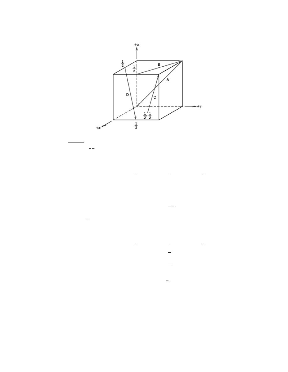
Excerpts from this work may be reproduced by instructors for distribution on a not-for-profit basis for testing or instructional purposes only to
students enrolled in courses for which the textbook has been adopted. Any other reproduction or translation of this work beyond that permitted
by Sections 107 or 108 of the 1976 United States Copyright Act without the permission of the copyright owner is unlawful.
3.31 Determine the indices for the directions shown in the following cubic unit cell:
Solution
Direction A is a
[ 0 1 1 ]direction, which determination is summarized as follows. We first of all position
the origin of the coordinate system at the tail of the direction vector; then in terms of this new coordinate system
x
y
z
Projections
0a
–b
–c
Projections in terms of a, b, and c
0
–1
–1
Reduction to integers
not necessary
Enclosure
[ 0 1 1 ]
Direction B is a
[ 2 10] direction, which determination is summarized as follows. We first of all position
the origin of the coordinate system at the tail of the direction vector; then in terms of this new coordinate system
x
y
z
Projections
–a
b
2
0c
Projections in terms of a, b, and c
–1
1
2
0
Reduction to integers
–2
1
0
Enclosure
[ 2 10]
Direction C is a [112] direction, which determination is summarized as follows. We first of all position the
origin of the coordinate system at the tail of the direction vector; then in terms of this new coordinate system
Excerpts from this work may be reproduced by instructors for distribution on a not-for-profit basis for testing or instructional purposes only to
students enrolled in courses for which the textbook has been adopted. Any other reproduction or translation of this work beyond that permitted
by Sections 107 or 108 of the 1976 United States Copyright Act without the permission of the copyright owner is unlawful.
x
y
z
Projections
a
2
b
2
c
Projections in terms of a, b, and c
1
2
1
2
1
Reduction to integers
1
1
2
Enclosure
[112]
Direction D is a
[112 ] direction, which determination is summarized as follows. We first of all position
the origin of the coordinate system at the tail of the direction vector; then in terms of this new coordinate system
x
y
z
Projections
a
2
b
2
–c
Projections in terms of a, b, and c
1
2
1
2
–1
Reduction to integers
1
1
–2
Enclosure
[112 ]
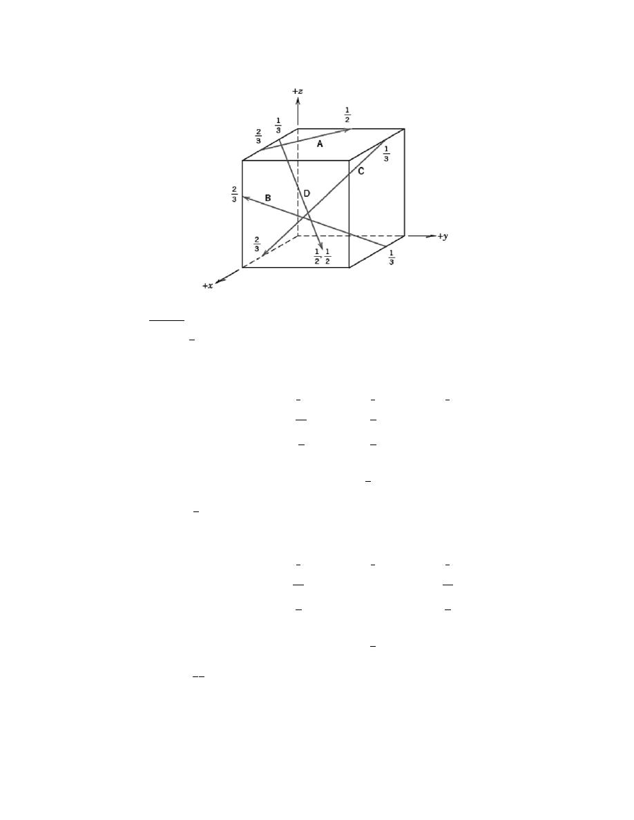
Excerpts from this work may be reproduced by instructors for distribution on a not-for-profit basis for testing or instructional purposes only to
students enrolled in courses for which the textbook has been adopted. Any other reproduction or translation of this work beyond that permitted
by Sections 107 or 108 of the 1976 United States Copyright Act without the permission of the copyright owner is unlawful.
3.32 Determine the indices for the directions shown in the following cubic unit cell:
Solution
Direction A is a
[ 4 30] direction, which determination is summarized as follows. We first of all position
the origin of the coordinate system at the tail of the direction vector; then in terms of this new coordinate system
x
y
z
Projections
–
2a
3
b
2
0c
Projections in terms of a, b, and c
–
2
3
1
2
0
Reduction to integers
–4
3
0
Enclosure
[ 4 30]
Direction B is a
[ 23 2] direction, which determination is summarized as follows. We first of all position
the origin of the coordinate system at the tail of the direction vector; then in terms of this new coordinate system
x
y
z
Projections
2a
3
–b
2c
3
Projections in terms of a, b, and c
2
3
–1
2
3
Reduction to integers
2
–3
2
Enclosure
[ 23 2]
Direction C is a
[13 3 ]
direction, which determination is summarized as follows. We first of all position
the origin of the coordinate system at the tail of the direction vector; then in terms of this new coordinate system
Excerpts from this work may be reproduced by instructors for distribution on a not-for-profit basis for testing or instructional purposes only to
students enrolled in courses for which the textbook has been adopted. Any other reproduction or translation of this work beyond that permitted
by Sections 107 or 108 of the 1976 United States Copyright Act without the permission of the copyright owner is unlawful.
x
y
z
Projections
a
3
–b
–c
Projections in terms of a, b, and c
1
3
–1
–1
Reduction to integers
1
–3
–3
Enclosure
[13 3 ]
Direction D is a
[136 ] direction, which determination is summarized as follows. We first of all position
the origin of the coordinate system at the tail of the direction vector; then in terms of this new coordinate system
x
y
z
Projections
a
6
b
2
–c
Projections in terms of a, b, and c
1
6
1
2
–1
Reduction to integers
1
3
–6
Enclosure
[136 ]

Excerpts from this work may be reproduced by instructors for distribution on a not-for-profit basis for testing or instructional purposes only to
students enrolled in courses for which the textbook has been adopted. Any other reproduction or translation of this work beyond that permitted
by Sections 107 or 108 of the 1976 United States Copyright Act without the permission of the copyright owner is unlawful.
3.33 For tetragonal crystals, cite the indices of directions that are equivalent to each of the following
directions:
(a) [001]
(b) [110]
(c) [010]
Solution
For tetragonal crystals a = b
≠ c and α = β = γ = 90°; therefore, projections along the x and y axes are
equivalent, which are not equivalent to projections along the z axis.
(a) Therefore, for the [001] direction, there is only one equivalent direction:
[ 00 1 ].
(b) For the [110] direction, equivalent directions are as follows:
[ 1 1 0] ,
[ 1 10] , and
[1 1 0]
(b) Also, for the [010] direction, equivalent directions are the following:
[ 0 1 0] ,
[100]
, and
[ 1 00] .

Excerpts from this work may be reproduced by instructors for distribution on a not-for-profit basis for testing or instructional purposes only to
students enrolled in courses for which the textbook has been adopted. Any other reproduction or translation of this work beyond that permitted
by Sections 107 or 108 of the 1976 United States Copyright Act without the permission of the copyright owner is unlawful.
3.34 Convert the [100] and [111] directions into the four-index Miller–Bravais scheme for hexagonal unit
cells.
Solution
For [100]
u' = 1,
v' = 0,
w' = 0
From Equations 3.6
u =
1
3
(2u'
− v' ) =
1
3
[(2)(1)
− 0] =
2
3
v =
1
3
(2vÕ
− uÕ) =
1
3
[(2)(0)
− 1] = −
1
3
t =
− (u + v) = −
2
3
−
1
3
= −
1
3
w = w' = 0
It is necessary to multiply these numbers by 3 in order to reduce them to the lowest set of integers. Thus, the
direction is represented as [uvtw] =
[ 2 1 1 0] .
For [111], u' = 1, v' = 1, and w' = 1; therefore,
u =
1
3
[(2)(1)
− 1] =
1
3
v =
1
3
[(2)(1)
− 1] =
1
3
t =
−
1
3
+
1
3
= −
2
3
w = 1

Excerpts from this work may be reproduced by instructors for distribution on a not-for-profit basis for testing or instructional purposes only to
students enrolled in courses for which the textbook has been adopted. Any other reproduction or translation of this work beyond that permitted
by Sections 107 or 108 of the 1976 United States Copyright Act without the permission of the copyright owner is unlawful.
If we again multiply these numbers by 3, then u = 1, v = 1, t = -2, and w = 3. Thus, the direction is represented as
Thus, the direction is represented as [uvtw] =
[112 3] .
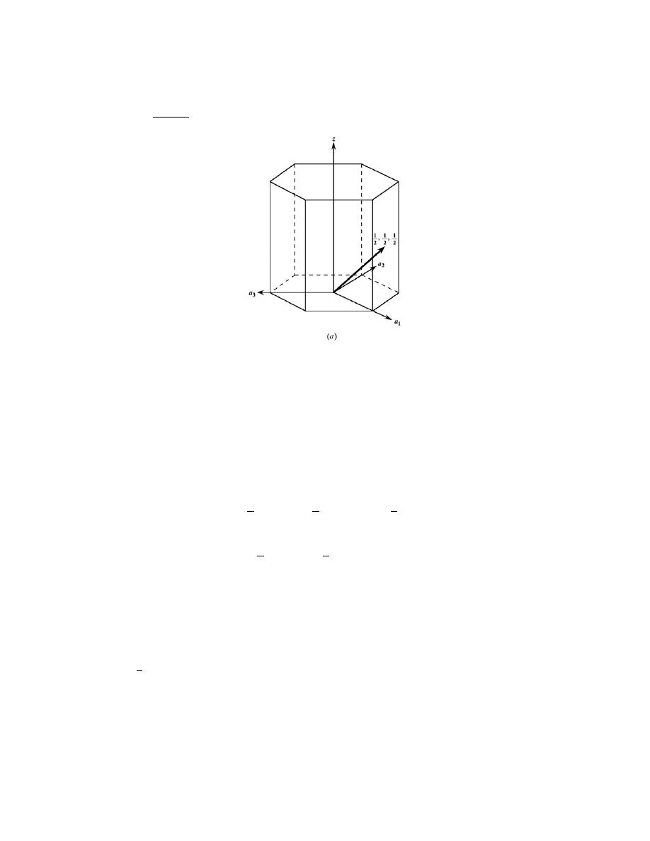
Excerpts from this work may be reproduced by instructors for distribution on a not-for-profit basis for testing or instructional purposes only to
students enrolled in courses for which the textbook has been adopted. Any other reproduction or translation of this work beyond that permitted
by Sections 107 or 108 of the 1976 United States Copyright Act without the permission of the copyright owner is unlawful.
3.35 Determine indices for the directions shown in the following hexagonal unit cells:
Solution
(a) For this direction, projections on the a
1
, a
2
, and z axes are a, a/2, and c/2, or, in terms of a and c the
projections are 1, 1/2, and 1/2, which when multiplied by the factor 2 become the smallest set of integers: 2, 1, and
1. This means that
u’ = 2
v’ = 1
w’ = 1
Now, from Equations 3.6, the u, v, t, and w indices become
u =
1
3
(2u'
− v' ) =
1
3
(2)(2)
− (1)
[
]
=
3
3
= 1
v =
1
3
(2vÕ
− uÕ) =
1
3
(2)(1)
− (2)
[
]
= 0
t
= − (u + v) = − 1 + 0
(
)
= −1
w = w’ = 1
No reduction is necessary inasmuch as all of these indices are integers; therefore, this direction in the four-index
scheme is
[10 1 1]
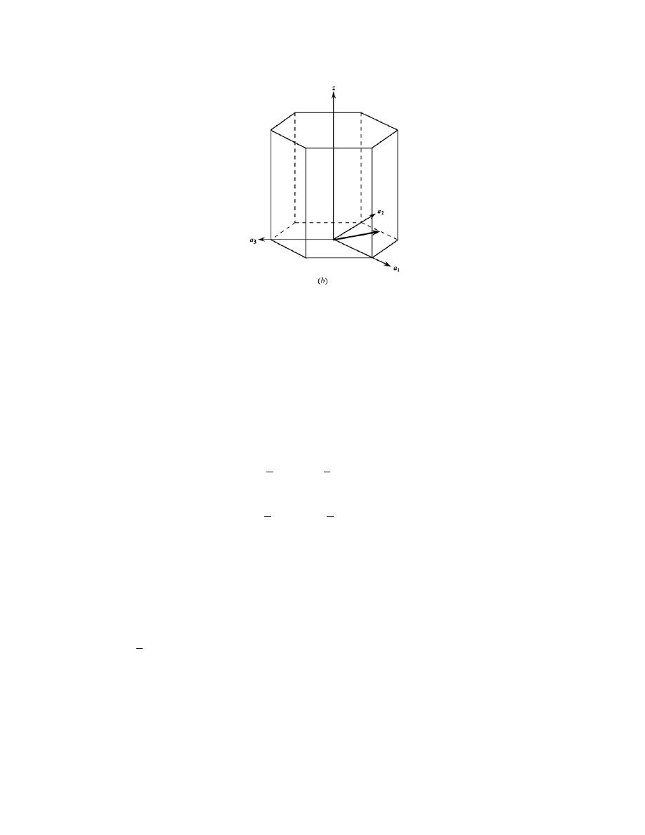
Excerpts from this work may be reproduced by instructors for distribution on a not-for-profit basis for testing or instructional purposes only to
students enrolled in courses for which the textbook has been adopted. Any other reproduction or translation of this work beyond that permitted
by Sections 107 or 108 of the 1976 United States Copyright Act without the permission of the copyright owner is unlawful.
(b) For this direction, projections on the a
1
, a
2
, and z axes are a/2, a, and 0c, or, in terms of a and c the
projections are 1/2, 1, and 0, which when multiplied by the factor 2 become the smallest set of integers: 1, 2, and 0
This means that
u’ = 1
v’ = 2
w’ = 0
Now, from Equations 3.6, the u, v, t, and w indices become
u
=
1
3
(2u'
− v) =
1
3
(2)(1)
− 2
[
]
= 0
v
=
1
3
(2v'
− u' ) =
1
3
(2)(2)
− 1
[
]
= 1
t
= − (u+ v) = − 0 + 1
(
)
= −1
w
= w' = 0
No reduction is necessary inasmuch as all of these indices are integers; therefore, this direction in the four-index
scheme is
[ 01 1 0] .
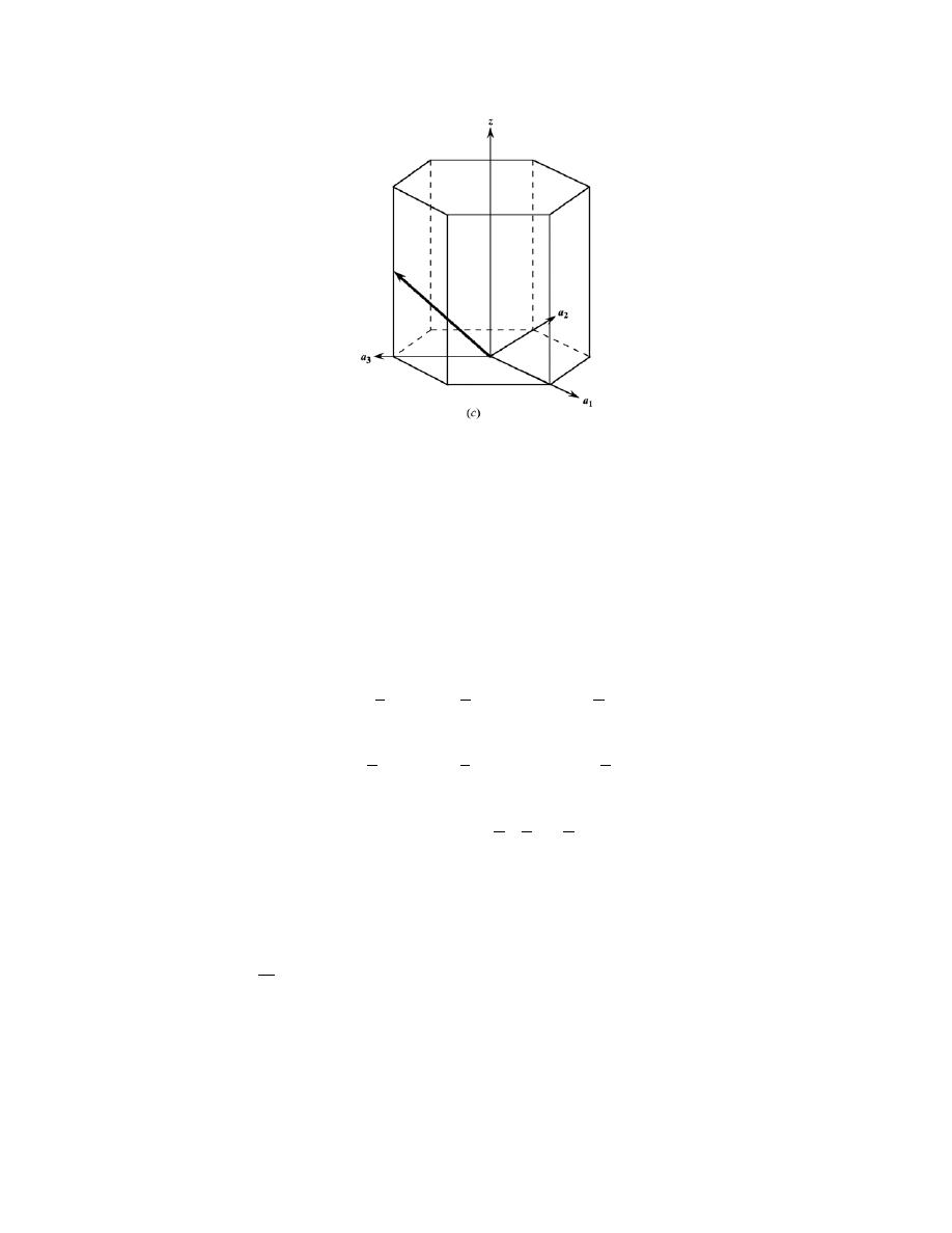
Excerpts from this work may be reproduced by instructors for distribution on a not-for-profit basis for testing or instructional purposes only to
students enrolled in courses for which the textbook has been adopted. Any other reproduction or translation of this work beyond that permitted
by Sections 107 or 108 of the 1976 United States Copyright Act without the permission of the copyright owner is unlawful.
(c) For this direction projections on the a
1
, a
2
, and z axes are
−a, −a, and c/2, or, in terms of a and c the
projections are
−1, −1, and 1/2, which when multiplied by the factor 2 become the smallest set of integers: −2, −2,
and 1. This means that
u’ =
−2
v’ =
−2
w’ = 1
Now, from Equations 3.6, the u, v, t, and w indices become
u
=
1
3
(2u'
− v) =
1
3
(2)(
−2) − (−2)
[
]
=−
2
3
v
=
1
3
(2v'
− u' ) =
1
3
(2)(
−2) − (−2)
[
]
= −
2
3
t
= − (u+ v) = − −
2
3
−
2
3
=
4
3
w
= w' = 1
Now, in order to get the lowest set of integers, it is necessary to multiply all indices by the factor 3, with the result
that this direction is a
[ 2 2 43]
direction.
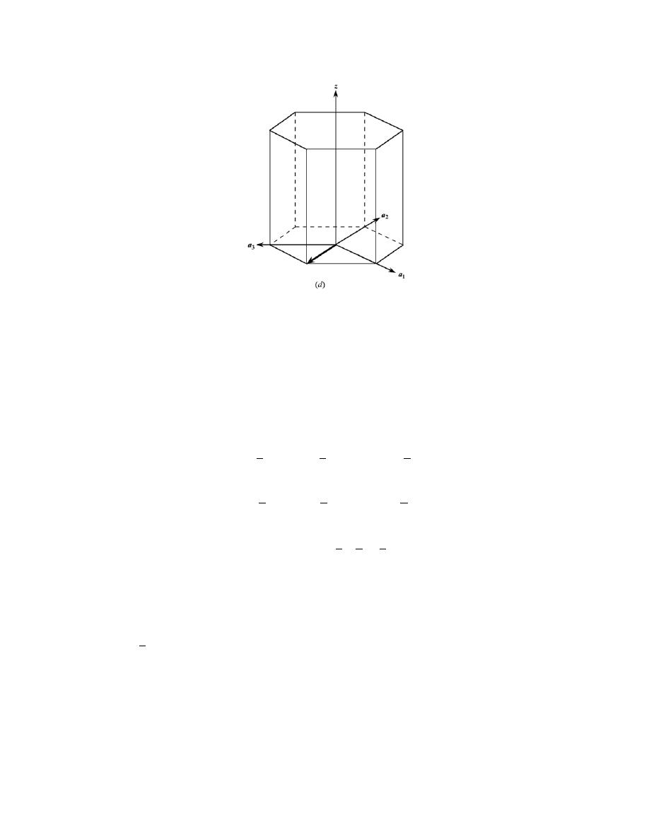
Excerpts from this work may be reproduced by instructors for distribution on a not-for-profit basis for testing or instructional purposes only to
students enrolled in courses for which the textbook has been adopted. Any other reproduction or translation of this work beyond that permitted
by Sections 107 or 108 of the 1976 United States Copyright Act without the permission of the copyright owner is unlawful.
(d) For this direction, projections on the a
1
, a
2
, and z axes are 0a,
−a, and 0c, or, in terms of a and c the
projections are 0, -1, and 0. This means that
u’ = 0
v’ =
−1
w’ = 0
Now, from Equations 3.6, the u, v, t, and w indices become
u
=
1
3
(2u'
− v' ) =
1
3
(2)(0)
− (−1)
[
]
=
1
3
v
=
1
3
(2v'
− u' ) =
1
3
(2)(
−1) − 0
[
]
=−
2
3
t
= − (u+ v) = −
1
3
−
2
3
=
1
3
w
= wÕ= 0
Now, in order to get the lowest set of integers, it is necessary to multiply all indices by the factor 3, with the result
that this is a
[12 10]
direction.
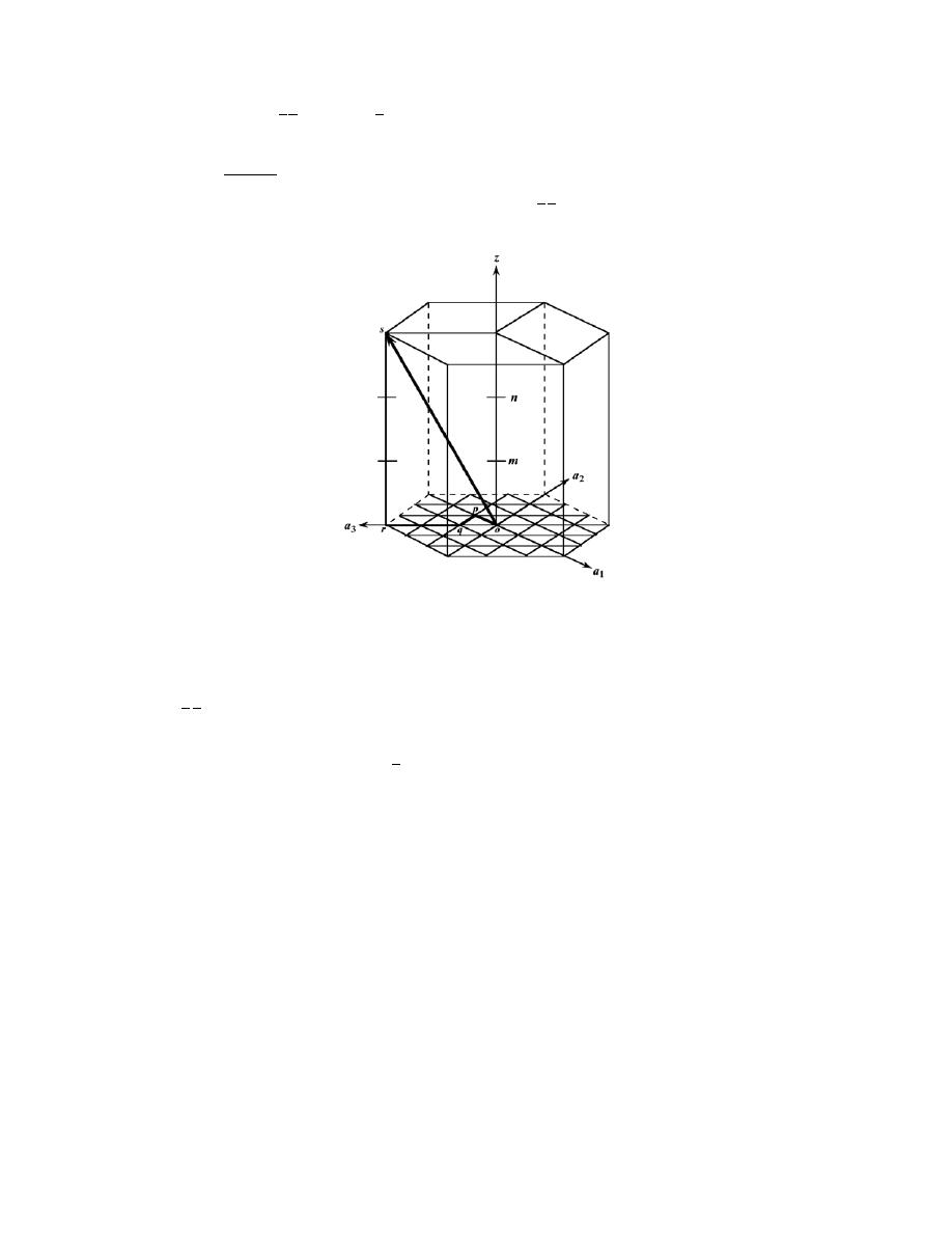
Excerpts from this work may be reproduced by instructors for distribution on a not-for-profit basis for testing or instructional purposes only to
students enrolled in courses for which the textbook has been adopted. Any other reproduction or translation of this work beyond that permitted
by Sections 107 or 108 of the 1976 United States Copyright Act without the permission of the copyright owner is unlawful.
3.36 Sketch the
[1 1 23] and
[101 0] directions in a hexagonal unit cell.
Solution
The first portion of this problem asks that we plot the
[ 1 1 23] within a hexagonal unit cell. Below is
shown this direction plotted within a hexagonal unit cell having a reduced-scale coordinate scheme.
For this direction, projections on the a
1
, a
2
, a
3
, and c axes are respectively,
−1, −1, 2, and 3, respectively. In
plotting this direction, we begin at the origin of the coordinate system, point o. From here we proceed 1 unit
distance along the
−a
1
axis (to point p), from here 1 unit distance parallel to
−a
2
axis (to point q), then 2 unit
distances parallel (or along) the a
3
axis (to point r), and finally, 3 unit distances parallel to the z axis (to point s).
Thus, the
[ 1 1 23] direction is that vector that extends from point o to point s as shown.
Now we are asked to plot the
[10 1 0] within a hexagonal unit cell. In the figure below is plotted this
direction within a hexagonal unit cell having a reduced-scale coordinate scheme.
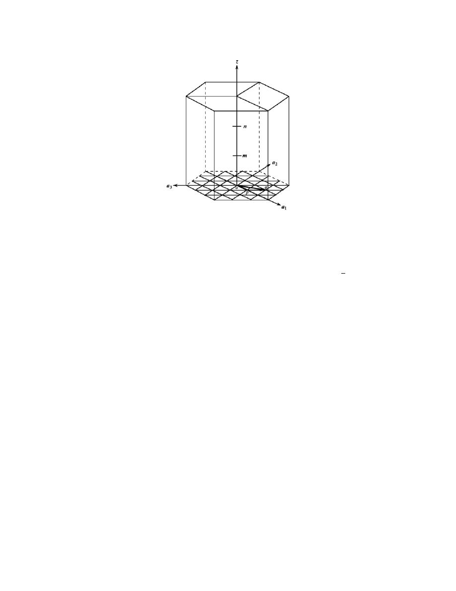
Excerpts from this work may be reproduced by instructors for distribution on a not-for-profit basis for testing or instructional purposes only to
students enrolled in courses for which the textbook has been adopted. Any other reproduction or translation of this work beyond that permitted
by Sections 107 or 108 of the 1976 United States Copyright Act without the permission of the copyright owner is unlawful.
For this direction, projections on the a
1
, a
2
, a
3
, and c axes are respectively, 1, 0,
−1, and 0, respectively. In plotting
this direction, we begin at the origin of the coordinate system, point o. From here we proceed 1 unit distance along
the a
1
axis (to point p). Since there is no projection on the a
2
axis it is not necessary to move parallel to this axis.
Therefore, from point p we proceed 1 unit distance parallel to
−a
3
axis (to point q). And, finally, inasmuch as there
is no projection along the z axis, it is not necessary to move parallel to this axis. Thus, the
[10 1 0] direction is that
vector that extends from point o to point q as shown.

Excerpts from this work may be reproduced by instructors for distribution on a not-for-profit basis for testing or instructional purposes only to
students enrolled in courses for which the textbook has been adopted. Any other reproduction or translation of this work beyond that permitted
by Sections 107 or 108 of the 1976 United States Copyright Act without the permission of the copyright owner is unlawful.
3.37 Using Equations 3.6a, 3.6b, 3.6c, and 3.6d, derive expressions for each of the three primed indices
set (u
′, v′, and w′) in terms of the four unprimed indices (u, v, t, and w).
Solution
It is first necessary to do an expansion of Equation 3.6a as
u
=
1
3
(2u'
− v) =
2u'
3
−
v'
3
And solving this expression for v’ yields
v'
= 2u' − 3u
Now, substitution of this expression into Equation 3.6b gives
v
=
1
3
(2vÕ
− uÕ) =
1
3
(2)(2uÕ
− 3u) − uÕ
[
]
= uÕ− 2u
Or
u'
= v + 2u
And, solving for v from Equation 3.6c leads to
v
= − (u + t)
which, when substituted into the above expression for u’ yields
u'
= v + 2u = − u − t + 2u = u − t
In solving for an expression for v’, we begin with the one of the above expressions for this parameter—i.e.,
v'
= 2u' − 3u
Now, substitution of the above expression for u’ into this equation leads to
vÕ
= 2uÕ− 3u = (2)(u − t) − 3u = − u −2t

Excerpts from this work may be reproduced by instructors for distribution on a not-for-profit basis for testing or instructional purposes only to
students enrolled in courses for which the textbook has been adopted. Any other reproduction or translation of this work beyond that permitted
by Sections 107 or 108 of the 1976 United States Copyright Act without the permission of the copyright owner is unlawful.
And solving for u from Equation 3.6c gives
u
= − v − t
which, when substituted in the previous equation results in the following expression for v’
vÕ
= − u −2t = − (− v − t) − 2t = v − t
And, of course from Equation 3.6d
w’ = w

Excerpts from this work may be reproduced by instructors for distribution on a not-for-profit basis for testing or instructional purposes only to
students enrolled in courses for which the textbook has been adopted. Any other reproduction or translation of this work beyond that permitted
by Sections 107 or 108 of the 1976 United States Copyright Act without the permission of the copyright owner is unlawful.
Crystallographic Planes
3.38 (a) Draw an orthorhombic unit cell, and within that cell a (210) plane.
(b) Draw a monoclinic unit cell, and within that cell a (002) plane.
Solution
(a) We are asked to draw a (210) plane within an orthorhombic unit cell. First remove the three indices
from the parentheses, and take their reciprocals--
i.e., 1/2, 1, and ∞. This means that the plane intercepts the x-axis
at a/2, the y-axis at b, and parallels the z-axis. The plane that satisfies these requirements has been drawn within the
orthorhombic unit cell below. (For orthorhombic, a
≠ b ≠ c, and α = β = γ = 90°.)
(b) A (002) plane is drawn within the monoclinic cell shown below. We first remove the parentheses and
take the reciprocals of the indices; this gives
∞, ∞, and 1/2. Thus, the (002) plane parallels both x- and y-axes, and
intercepts the z-axis at a/2, as indicated in the drawing. (For monoclinic, a
≠ b ≠ c, and α = γ = 90° ≠ β.)
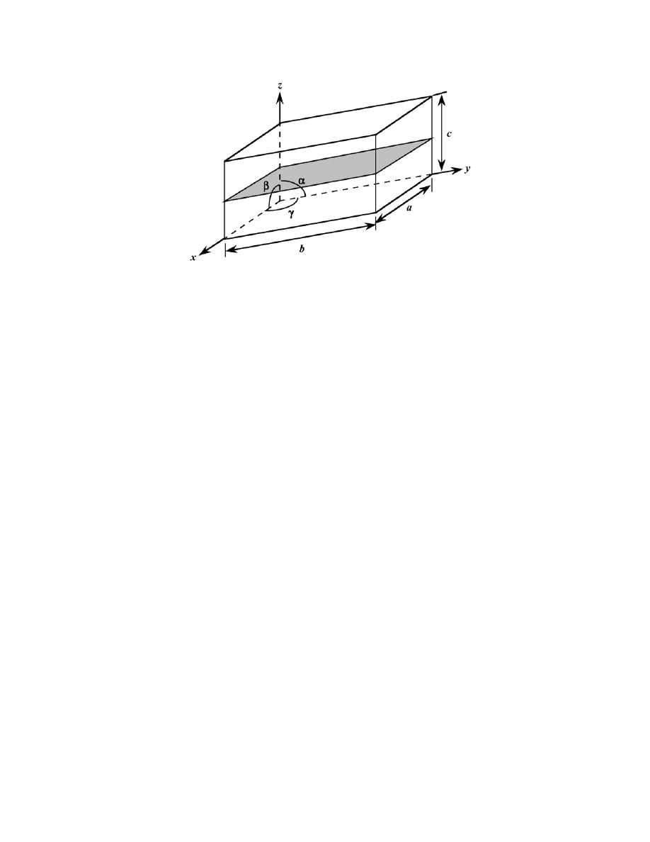
Excerpts from this work may be reproduced by instructors for distribution on a not-for-profit basis for testing or instructional purposes only to
students enrolled in courses for which the textbook has been adopted. Any other reproduction or translation of this work beyond that permitted
by Sections 107 or 108 of the 1976 United States Copyright Act without the permission of the copyright owner is unlawful.
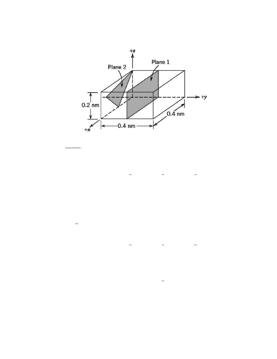
3.39 What are the indices for the two planes drawn in the sketch below?
Solution
Plane 1 is a (020) plane. The determination of its indices is summarized below.
x
y
z
Intercepts
∞a
b/2
∞c
Intercepts in terms of a, b, and c
∞
1/2
∞
Reciprocals of intercepts
0
2
0
Enclosure
(020)
Plane 2 is a
(22 1)
plane, as summarized below.
x
y
z
Intercepts
a/2
-b/2
c
Intercepts in terms of a, b, and c
1/2
-1/2
1
Reciprocals of intercepts
2
-2
1
Enclosure
(22 1)
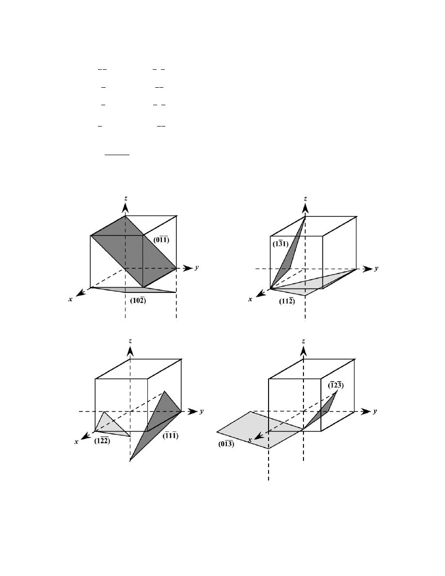
Excerpts from this work may be reproduced by instructors for distribution on a not-for-profit basis for testing or instructional purposes only to
students enrolled in courses for which the textbook has been adopted. Any other reproduction or translation of this work beyond that permitted
by Sections 107 or 108 of the 1976 United States Copyright Act without the permission of the copyright owner is unlawful.
3.40 Sketch within a cubic unit cell the following planes:
(a)
(01 1 ) ,
(e)
(1 11 ) ,
(b)
(112 ) ,
(f)
(12 2 ) ,
(c)
(102 ) ,
(g)
(1 23 ),
(d)
(13 1) ,
(h)
(01 3 )
Solution
The planes called for are plotted in the cubic unit cells shown below.
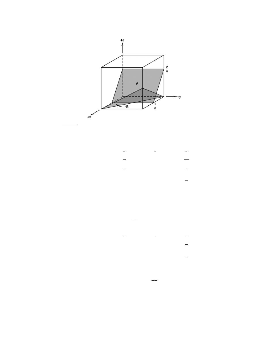
Excerpts from this work may be reproduced by instructors for distribution on a not-for-profit basis for testing or instructional purposes only to
students enrolled in courses for which the textbook has been adopted. Any other reproduction or translation of this work beyond that permitted
by Sections 107 or 108 of the 1976 United States Copyright Act without the permission of the copyright owner is unlawful.
3.41 Determine the Miller indices for the planes shown in the following unit cell:
Solution
For plane A we will leave the origin at the unit cell as shown; this is a (403) plane, as summarized below.
x
y
z
Intercepts
a
2
∞b
2c
3
Intercepts in terms of a, b, and c
1
2
∞
2
3
Reciprocals of intercepts
2
0
3
2
Reduction
4
0
3
Enclosure
(403)
For plane B we will move the origin of the unit cell one unit cell distance to the right along the y axis, and
one unit cell distance parallel to the x axis; thus, this is a
(1 1 2)
plane, as summarized below.
x
y
z
Intercepts
– a
– b
c
2
Intercepts in terms of a, b, and c
– 1
– 1
1
2
Reciprocals of intercepts
– 1
– 1
2
Reduction
(not necessary)
Enclosure
(1 1 2)
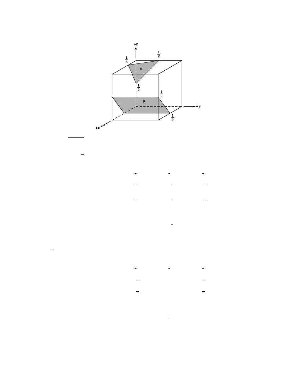
Excerpts from this work may be reproduced by instructors for distribution on a not-for-profit basis for testing or instructional purposes only to
students enrolled in courses for which the textbook has been adopted. Any other reproduction or translation of this work beyond that permitted
by Sections 107 or 108 of the 1976 United States Copyright Act without the permission of the copyright owner is unlawful.
3.42 Determine the Miller indices for the planes shown in the following unit cell:
Solution
For plane A we will move the origin of the coordinate system one unit cell distance to the upward along the
z axis; thus, this is a
(322 ) plane, as summarized below.
x
y
z
Intercepts
a
3
b
2
–
c
2
Intercepts in terms of a, b, and c
1
3
1
2
–
1
2
Reciprocals of intercepts
3
2
– 2
Reduction
(not necessary)
Enclosure
(322 )
For plane B we will move the original of the coordinate system on unit cell distance along the x axis; thus,
this is a
(1 01) plane, as summarized below.
x
y
z
Intercepts
–
a
2
∞b
c
2
Intercepts in terms of a, b, and c
–
1
2
∞
1
2
Reciprocals of intercepts
– 2
0
2
Reduction
– 1
0
1
Enclosure
(1 01)
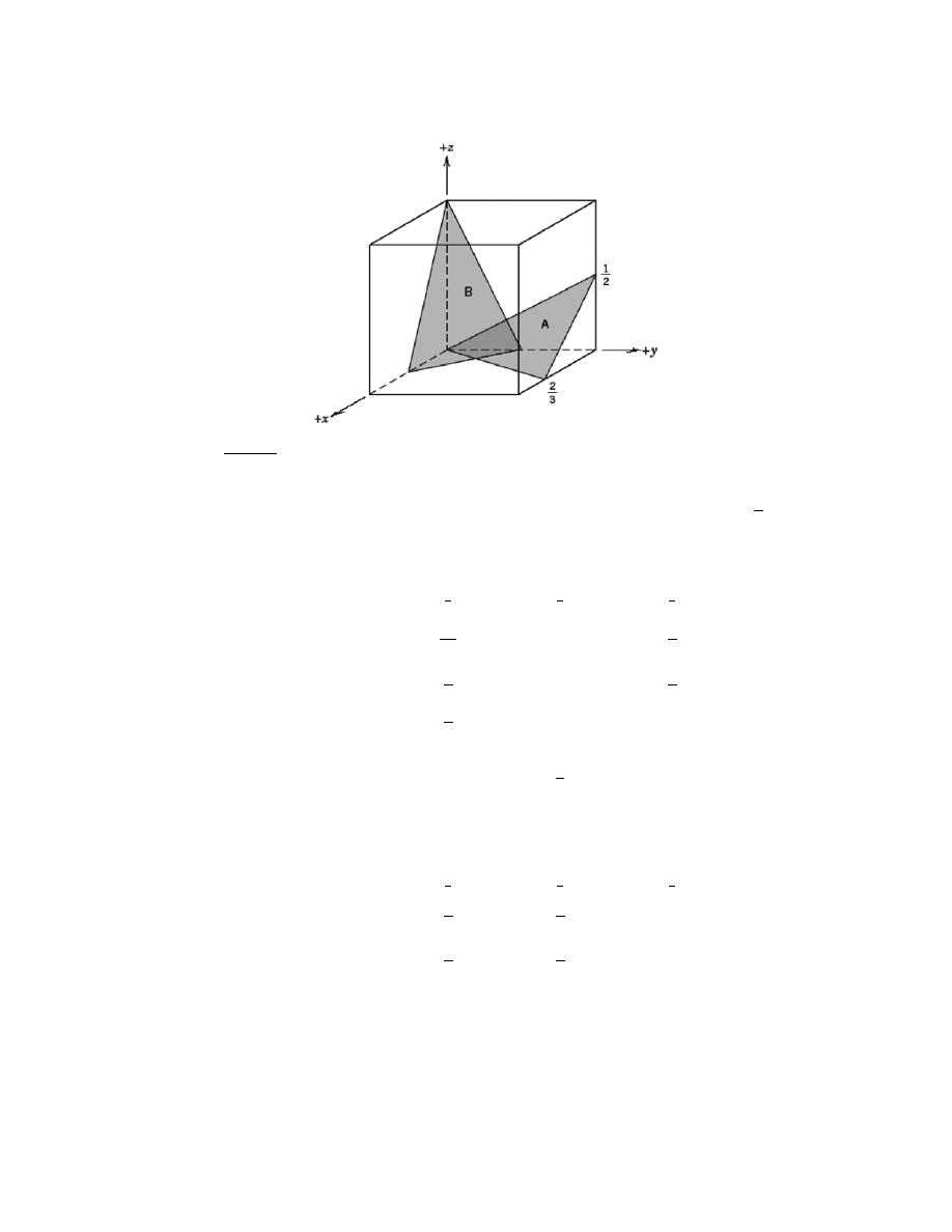
Excerpts from this work may be reproduced by instructors for distribution on a not-for-profit basis for testing or instructional purposes only to
students enrolled in courses for which the textbook has been adopted. Any other reproduction or translation of this work beyond that permitted
by Sections 107 or 108 of the 1976 United States Copyright Act without the permission of the copyright owner is unlawful.
3.43 Determine the Miller indices for the planes shown in the following unit cell:
Solution
For plane A since the plane passes through the origin of the coordinate system as shown, we will move the
origin of the coordinate system one unit cell distance to the right along the y axis; thus, this is a
(32 4) plane, as
summarized below.
x
y
z
Intercepts
2a
3
– b
c
2
Intercepts in terms of a, b, and c
2
3
– 1
1
2
Reciprocals of intercepts
3
2
– 1
2
Reduction
3
– 2
4
Enclosure
(32 4)
For plane B we will leave the origin at the unit cell as shown; this is a (221) plane, as summarized below.
x
y
z
Intercepts
a
2
b
2
c
Intercepts in terms of a, b, and c
1
2
1
2
1
Reciprocals of intercepts
2
2
1
Reduction
not necessary
Enclosure
(221)
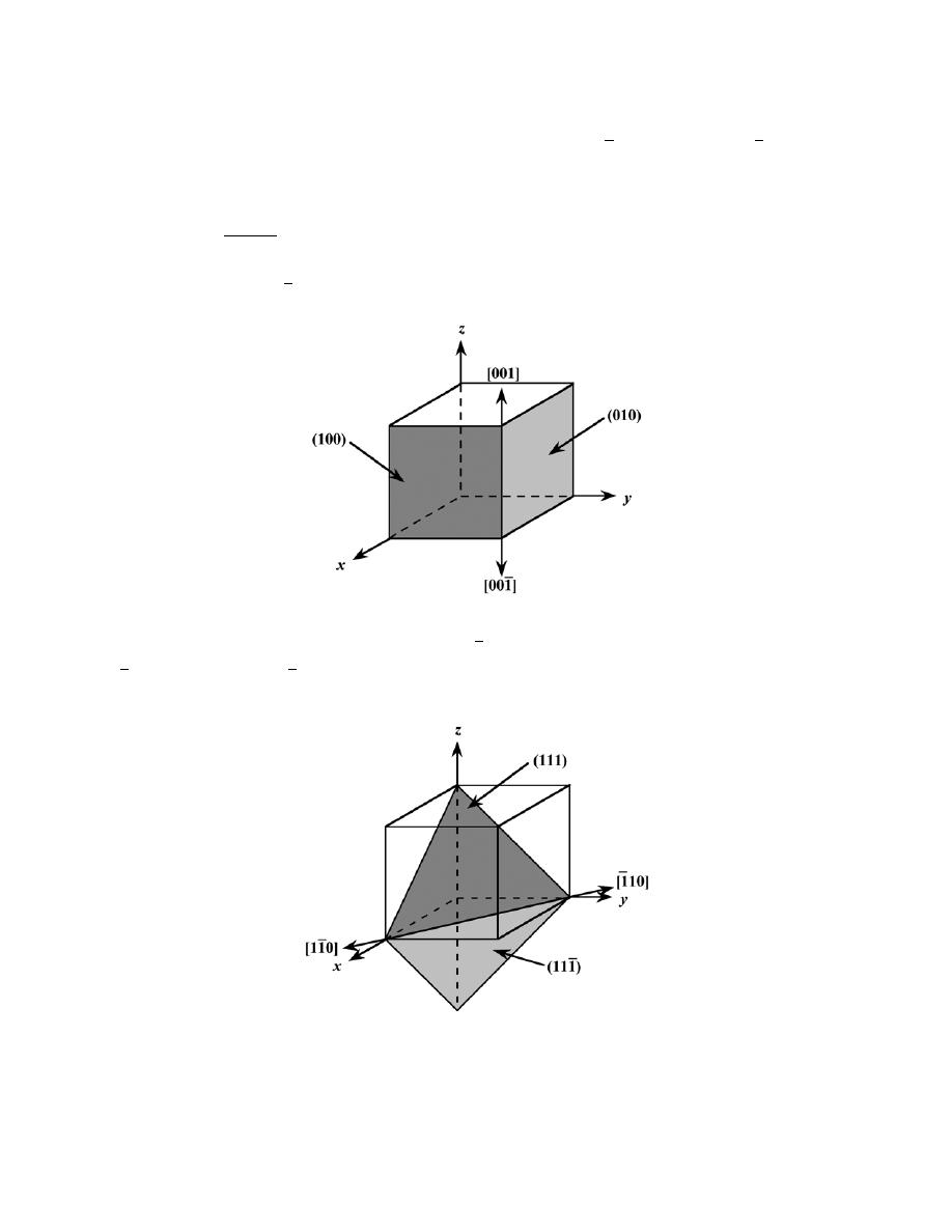
Excerpts from this work may be reproduced by instructors for distribution on a not-for-profit basis for testing or instructional purposes only to
students enrolled in courses for which the textbook has been adopted. Any other reproduction or translation of this work beyond that permitted
by Sections 107 or 108 of the 1976 United States Copyright Act without the permission of the copyright owner is unlawful.
3.44 Cite the indices of the direction that results from the intersection of each of the following pair of planes
within a cubic crystal: (a) (100) and (010) planes, (b) (111) and
(111 ) planes, and (c)
(101 ) and (001)
planes.
Solution
(a) In the figure below is shown (100) and (010) planes, and, as indicated, their intersection results in a [001],
or equivalently, a
[ 00 1 ] direction.
(b) In the figure below is shown (111) and
(11 1 ) planes, and, as indicated, their intersection results in a
[ 1 10] , or equivalently, a
[1 1 0] direction.
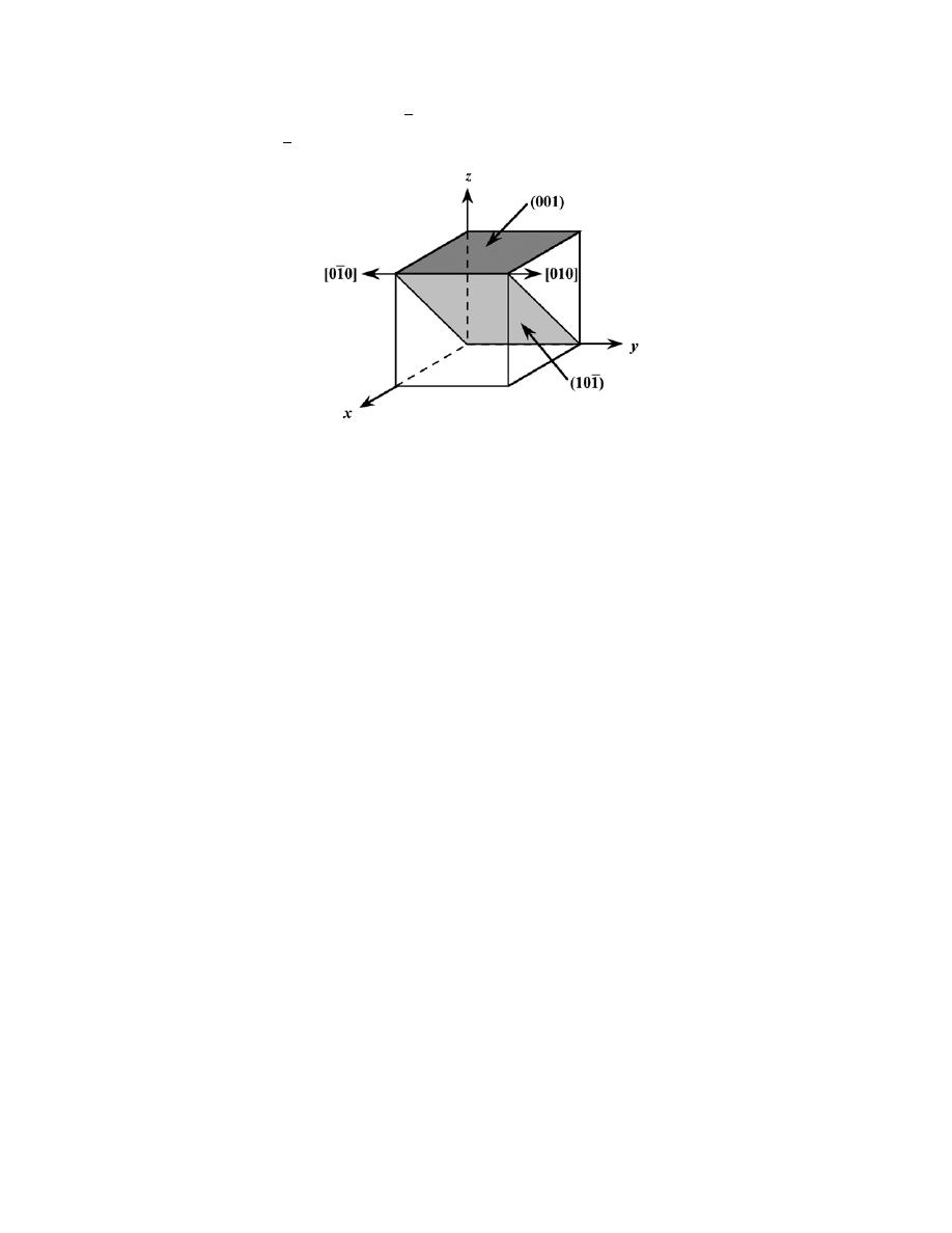
Excerpts from this work may be reproduced by instructors for distribution on a not-for-profit basis for testing or instructional purposes only to
students enrolled in courses for which the textbook has been adopted. Any other reproduction or translation of this work beyond that permitted
by Sections 107 or 108 of the 1976 United States Copyright Act without the permission of the copyright owner is unlawful.
(c) In the figure below is shown
(10 1 ) and (001) planes, and, as indicated, their intersection results in a
[010], or equivalently, a
[ 0 1 0] direction.
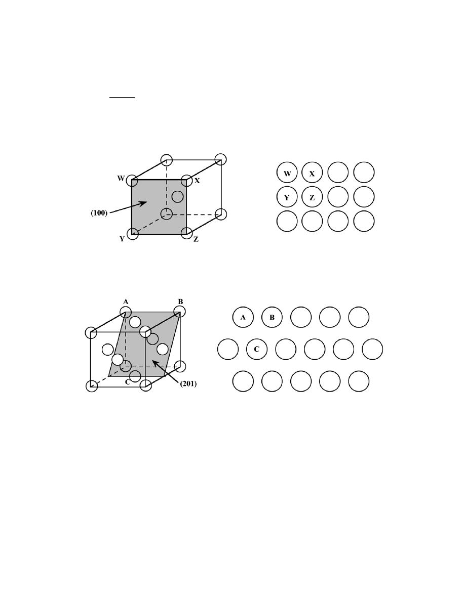
Excerpts from this work may be reproduced by instructors for distribution on a not-for-profit basis for testing or instructional purposes only to
students enrolled in courses for which the textbook has been adopted. Any other reproduction or translation of this work beyond that permitted
by Sections 107 or 108 of the 1976 United States Copyright Act without the permission of the copyright owner is unlawful.
3.45 Sketch the atomic packing of (a) the (100) plane for the BCC crystal structure, and (b) the (201)
plane for the FCC crystal structure (similar to Figures 3.10b and 3.11b).
Solution
(a) A BCC unit cell, its (100) plane, and the atomic packing of this plane are indicated below.
Corresponding atom positions in the two drawings are indicated by letters W, X, Y, and Z.
(b) An FCC unit cell, its (201) plane, and the atomic packing of this plane are indicated below.
Corresponding atom positions in the two drawing are indicated by the letters A, B, and C.
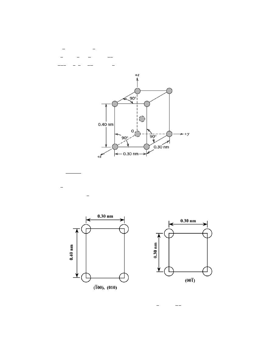
Excerpts from this work may be reproduced by instructors for distribution on a not-for-profit basis for testing or instructional purposes only to
students enrolled in courses for which the textbook has been adopted. Any other reproduction or translation of this work beyond that permitted
by Sections 107 or 108 of the 1976 United States Copyright Act without the permission of the copyright owner is unlawful.
3.46 Consider the reduced-sphere unit cell shown in Problem 3.20, having an origin of the coordinate
system positioned at the atom labeled with an O. For the following sets of planes, determine which are equivalent:
(a)
(001 ), (010), and,
(1 00)
(b)
(11 0) ,
(101 ) ,
(01 1), and
(1 1 0)
(c)
(1 1 1 ) ,
(1 11 ) ,
(1 1 1) , and
(11 1)
Solution
(a) The unit cell in Problem 3.20 is body-centered tetragonal. Of the three planes given in the problem
statement the
(1 00) and (010) are equivalent—that is, have the same atomic packing. The atomic packing for these
two planes as well as the
(00 1 ) are shown in the figure below.
(b) Of the four planes cited in the problem statement,
(1 1 0)
and
(1 1 0)
are equivalent to one another—
have the same atomic packing. The atomic arrangement of these planes is shown in the left drawing below.
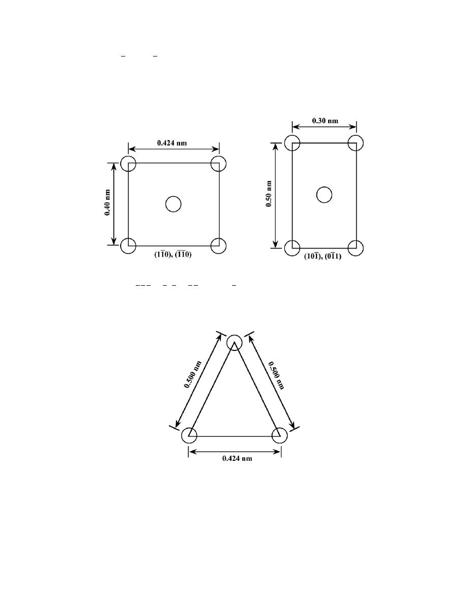
Excerpts from this work may be reproduced by instructors for distribution on a not-for-profit basis for testing or instructional purposes only to
students enrolled in courses for which the textbook has been adopted. Any other reproduction or translation of this work beyond that permitted
by Sections 107 or 108 of the 1976 United States Copyright Act without the permission of the copyright owner is unlawful.
Furthermore, the
(10 1 ) and
(0 1 1) are equivalent to each other (but not to the other pair of planes); their atomic
arrangement is represented in the other drawing. Note: the 0.424 nm dimension in the left-most drawing comes
from the relationship
(
0.30 nm
)
2
+
(
0.30 nm
)
2
[
]
1/ 2
. Likewise, the 0.500 nm dimension found in the right-most
drawing comes from
(
0.30 nm
)
2
+
(
0.40 nm
)
2
[
]
1/ 2
.
(c) All of the
(1 1 1 ) ,
(1 1 1 ) ,
(1 1 1) , and
(1 1 1) planes are equivalent, that is, have the same atomic
packing as illustrated in the following figure:
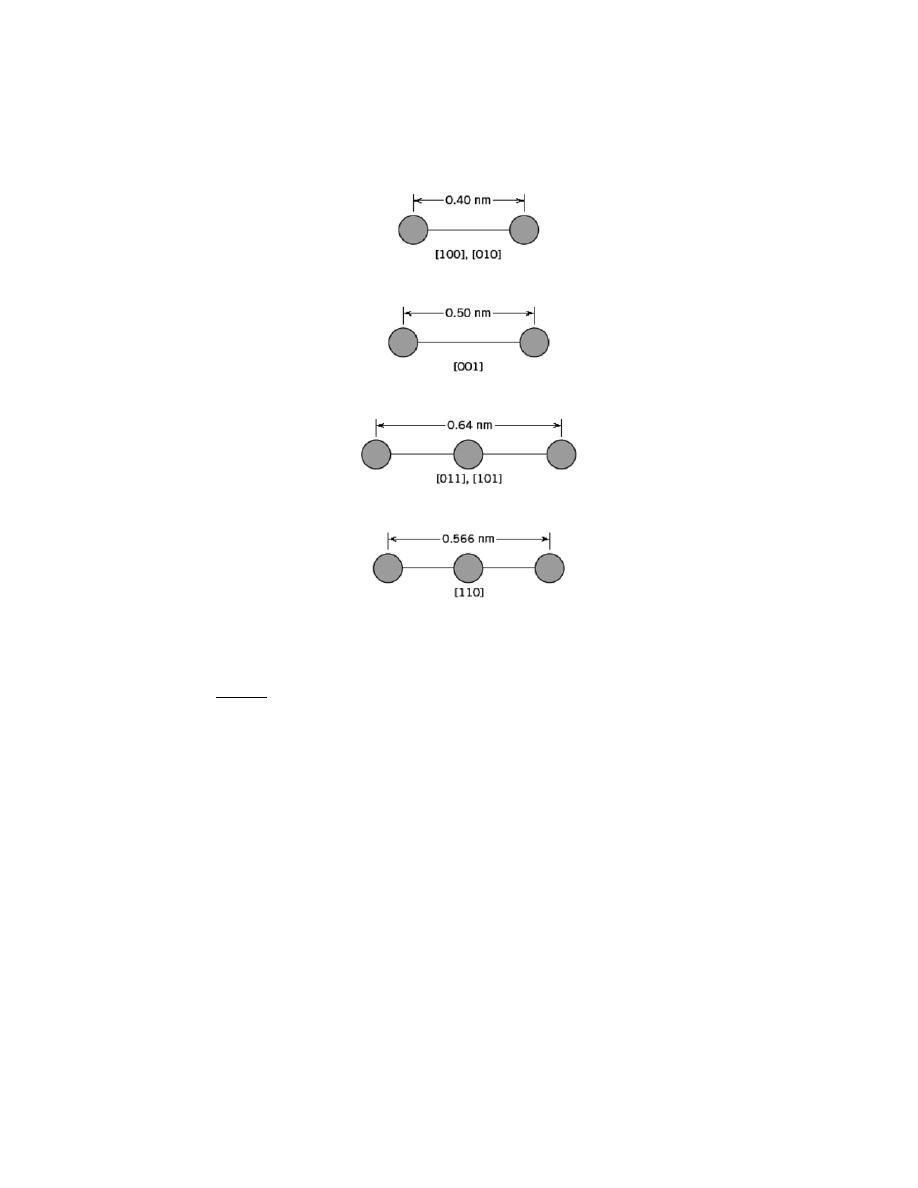
Excerpts from this work may be reproduced by instructors for distribution on a not-for-profit basis for testing or instructional purposes only to
students enrolled in courses for which the textbook has been adopted. Any other reproduction or translation of this work beyond that permitted
by Sections 107 or 108 of the 1976 United States Copyright Act without the permission of the copyright owner is unlawful.
3.47 Here are shown the atomic packing schemes for several different crystallographic directions for
some hypothetical metal. For each direction the circles represent only those atoms contained within a unit cell,
which circles are reduced from their actual size.
(a) To what crystal system does the unit cell belong?
(b) What would this crystal structure be called?
Solution
Below is constructed a unit cell using the six crystallographic directions that were provided in the problem.
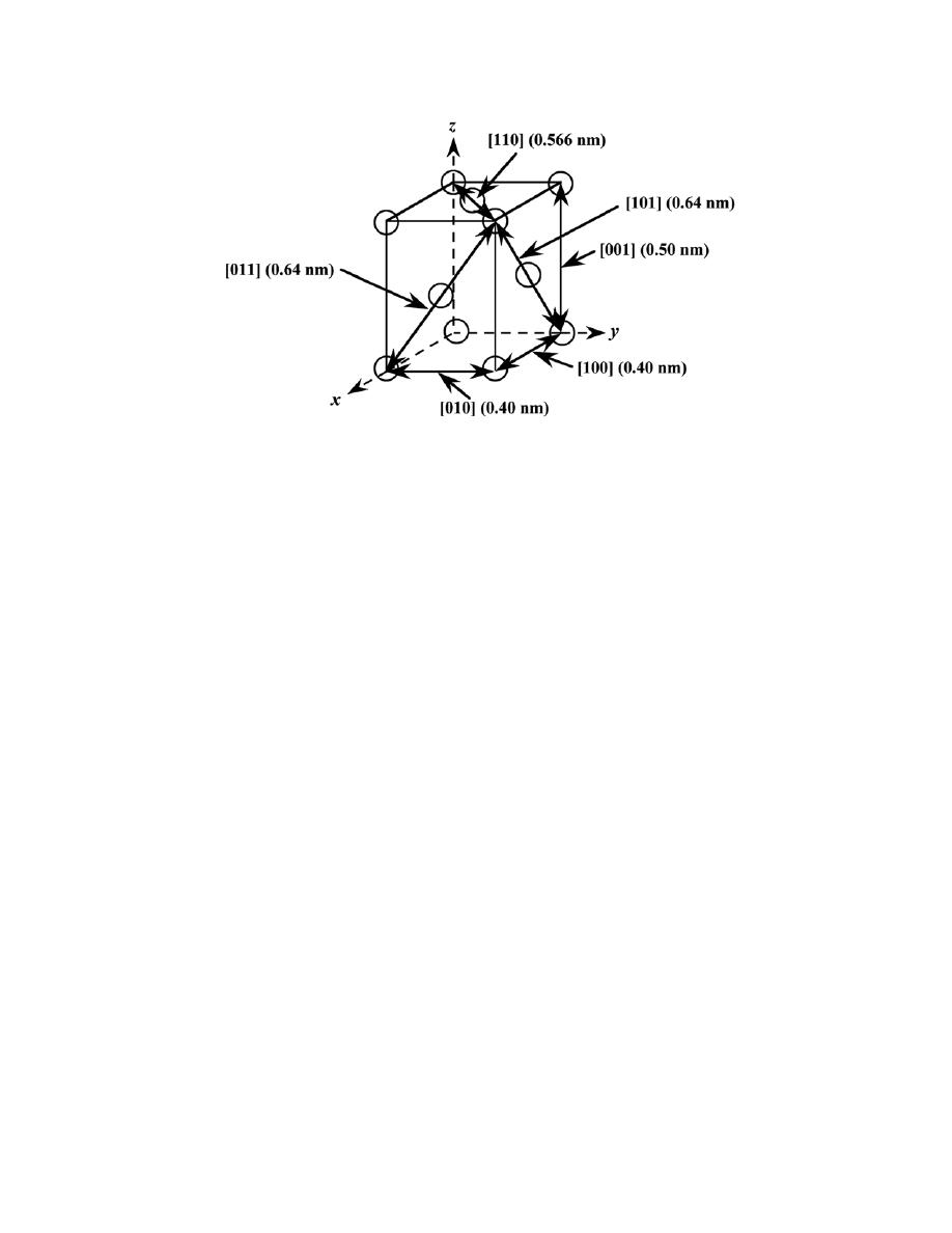
Excerpts from this work may be reproduced by instructors for distribution on a not-for-profit basis for testing or instructional purposes only to
students enrolled in courses for which the textbook has been adopted. Any other reproduction or translation of this work beyond that permitted
by Sections 107 or 108 of the 1976 United States Copyright Act without the permission of the copyright owner is unlawful.
(a) This unit cell belongs to the tetragonal system since a = b = 0.40 nm, c = 0.50 nm, and
α = β = γ = 90°.
(b) This crystal structure would be called face-centered tetragonal since the unit cell has tetragonal
symmetry, and an atom is located at each of the corners, as well as at the centers of all six unit cell faces. In the
figure above, atoms are only shown at the centers of three faces; however, atoms would also be situated at opposite
faces.
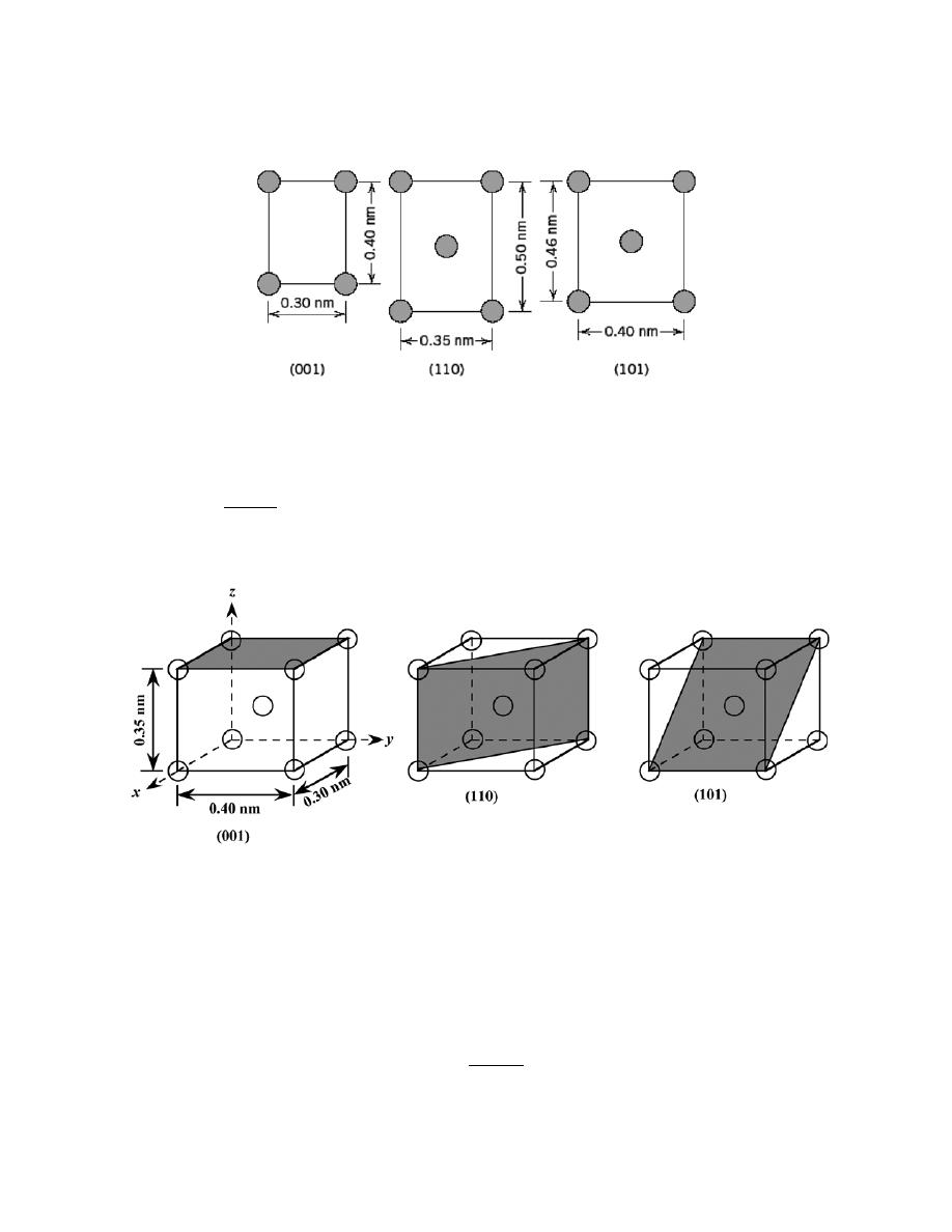
Excerpts from this work may be reproduced by instructors for distribution on a not-for-profit basis for testing or instructional purposes only to
students enrolled in courses for which the textbook has been adopted. Any other reproduction or translation of this work beyond that permitted
by Sections 107 or 108 of the 1976 United States Copyright Act without the permission of the copyright owner is unlawful.
3.48 Below are shown three different crystallographic planes for a unit cell of some hypothetical metal.
The circles represent atoms:
(a) To what crystal system does the unit cell belong?
(b) What would this crystal structure be called?
(c) If the density of this metal is 8.95 g/cm
3
, determine its atomic weight.
Solution
The unit cells constructed below show the three crystallographic planes that were provided in the problem
statement.
(a) This unit cell belongs to the orthorhombic crystal system since a = 0.30 nm, b = 0.40 nm, c = 0.35 nm,
and
α = β = γ = 90°.
(b) This crystal structure would be called body-centered orthorhombic since the unit cell has orthorhombic
symmetry, and an atom is located at each of the corners, as well as at the cell center.
(c) In order to compute its atomic weight, we employ Equation 3.5, with n = 2; thus
A =
ρV
C
N
A
n

Excerpts from this work may be reproduced by instructors for distribution on a not-for-profit basis for testing or instructional purposes only to
students enrolled in courses for which the textbook has been adopted. Any other reproduction or translation of this work beyond that permitted
by Sections 107 or 108 of the 1976 United States Copyright Act without the permission of the copyright owner is unlawful.
=
(
8.95 g/cm
3
)
(3.0)(4.0)(3.5)
(
× 10
-24
cm
3
/unit cell
)(
6.022
× 10
23
atoms/mol
)
2 atoms/unit cell
= 113.2 g/mol

Excerpts from this work may be reproduced by instructors for distribution on a not-for-profit basis for testing or instructional purposes only to
students enrolled in courses for which the textbook has been adopted. Any other reproduction or translation of this work beyond that permitted
by Sections 107 or 108 of the 1976 United States Copyright Act without the permission of the copyright owner is unlawful.
3.49 Convert the (010) and (101) planes into the four-index Miller–Bravais scheme for hexagonal unit
cells.
Solution
For (010), h = 0, k = 1, and l = 0, and, from Equation 3.7, the value of i is equal to
i
= − (h + k) = − (0 + 1) = −1
Therefore, the (010) plane becomes
(01 1 0) .
Now for the (101) plane, h = 1, k = 0, and l = 1, and computation of i using Equation 3.7 leads to
i
= − (h + k) = −[1 + 0] = −1
such that (101) becomes
(10 1 1) .
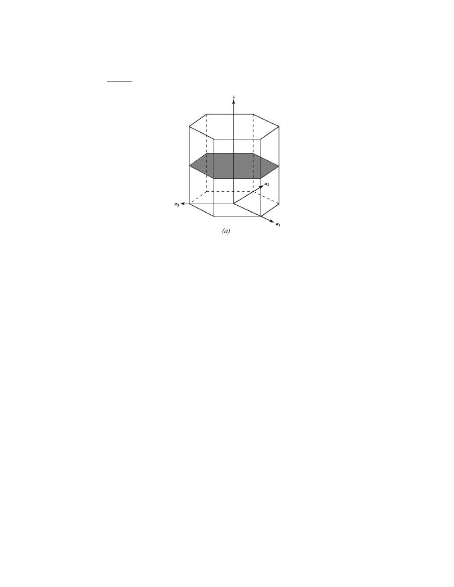
Excerpts from this work may be reproduced by instructors for distribution on a not-for-profit basis for testing or instructional purposes only to
students enrolled in courses for which the textbook has been adopted. Any other reproduction or translation of this work beyond that permitted
by Sections 107 or 108 of the 1976 United States Copyright Act without the permission of the copyright owner is unlawful.
3.50 Determine the indices for the planes shown in the hexagonal unit cells below:
Solution
(a) For this plane, intersections with the a
1
, a
2
, and z axes are
∞a, ∞a, and c/2 (the plane parallels both a
1
and a
2
axes). In terms of a and c these intersections are
∞, ∞, and ½, the respective reciprocals of which are 0, 0,
and 2. This means that
h = 0
k = 0
l = 2
Now, from Equation 3.7, the value of i is
i
= − (h + k) = −[0 + 0] = 0
Hence, this is a
(0002)
plane.
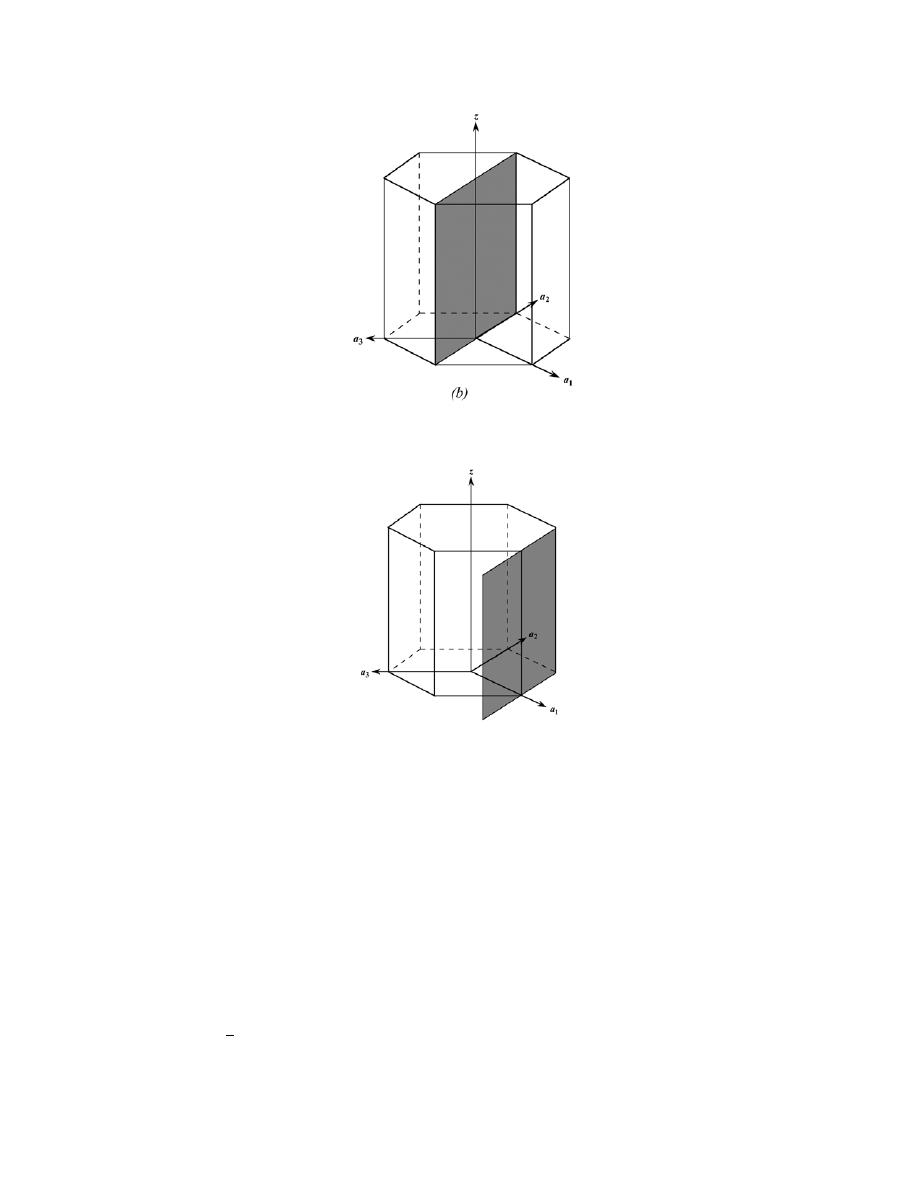
Excerpts from this work may be reproduced by instructors for distribution on a not-for-profit basis for testing or instructional purposes only to
students enrolled in courses for which the textbook has been adopted. Any other reproduction or translation of this work beyond that permitted
by Sections 107 or 108 of the 1976 United States Copyright Act without the permission of the copyright owner is unlawful.
(b) This plane passes through the origin of the coordinate axis system; therefore, we translate this plane
one unit distance along the x axis, per the sketch shown below:
At this point the plane intersects the a
1
, a
2
, and z axes at a,
∞a, and ∞c, respectively (the plane parallels both a
2
and
z axes). In terms of a and c these intersections are 1,
∞, and ∞, the respective reciprocals of which are 1, 0, and 0.
This means that
h = 1
k = 0
l = 0
Now, from Equation 3.7, the value of i is
i
= − (h + k) = − (1 + 0) = −1
Hence, this is a
(10 1 0)
plane.
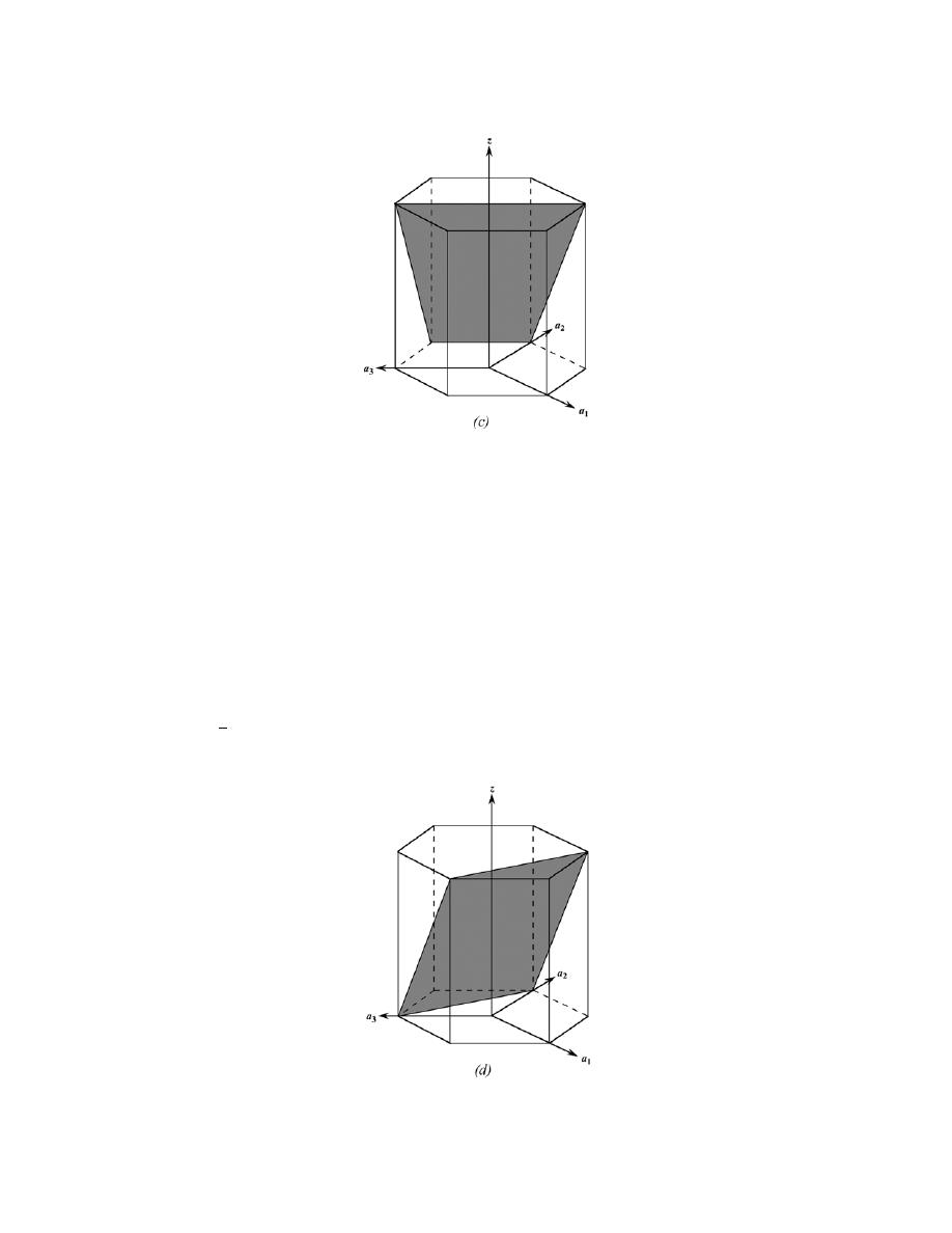
Excerpts from this work may be reproduced by instructors for distribution on a not-for-profit basis for testing or instructional purposes only to
students enrolled in courses for which the textbook has been adopted. Any other reproduction or translation of this work beyond that permitted
by Sections 107 or 108 of the 1976 United States Copyright Act without the permission of the copyright owner is unlawful.
(c) For this plane, intersections with the a
1
, a
2
, and z axes are –a, a, and c. In terms of a and c these
intersections are –1, 1, and 1, the respective reciprocals of which are 0, 1, and 1. This means that
h = –1
k = 1
l = 1
Now, from Equation 3.7, the value of i is
i
= − (h + k) = − (−1 + 1) = 0
Hence, this is a
(1 101) plane.

Excerpts from this work may be reproduced by instructors for distribution on a not-for-profit basis for testing or instructional purposes only to
students enrolled in courses for which the textbook has been adopted. Any other reproduction or translation of this work beyond that permitted
by Sections 107 or 108 of the 1976 United States Copyright Act without the permission of the copyright owner is unlawful.
(d) For this plane, intersections with the a
1
, a
2
, and z axes are –a/2, a, and c/2, respectively. In terms of a
and c these intersections are –1/2, 1, and 1/2, the respective reciprocals of which are –2, 1, and 2. This means that
h = –2
k = 1
l = 2
Now, from Equation 3.7, the value of i is
i
= − (h + k) = − (−2 + 1) = 1
Therefore, this is a
(2 112) plane.
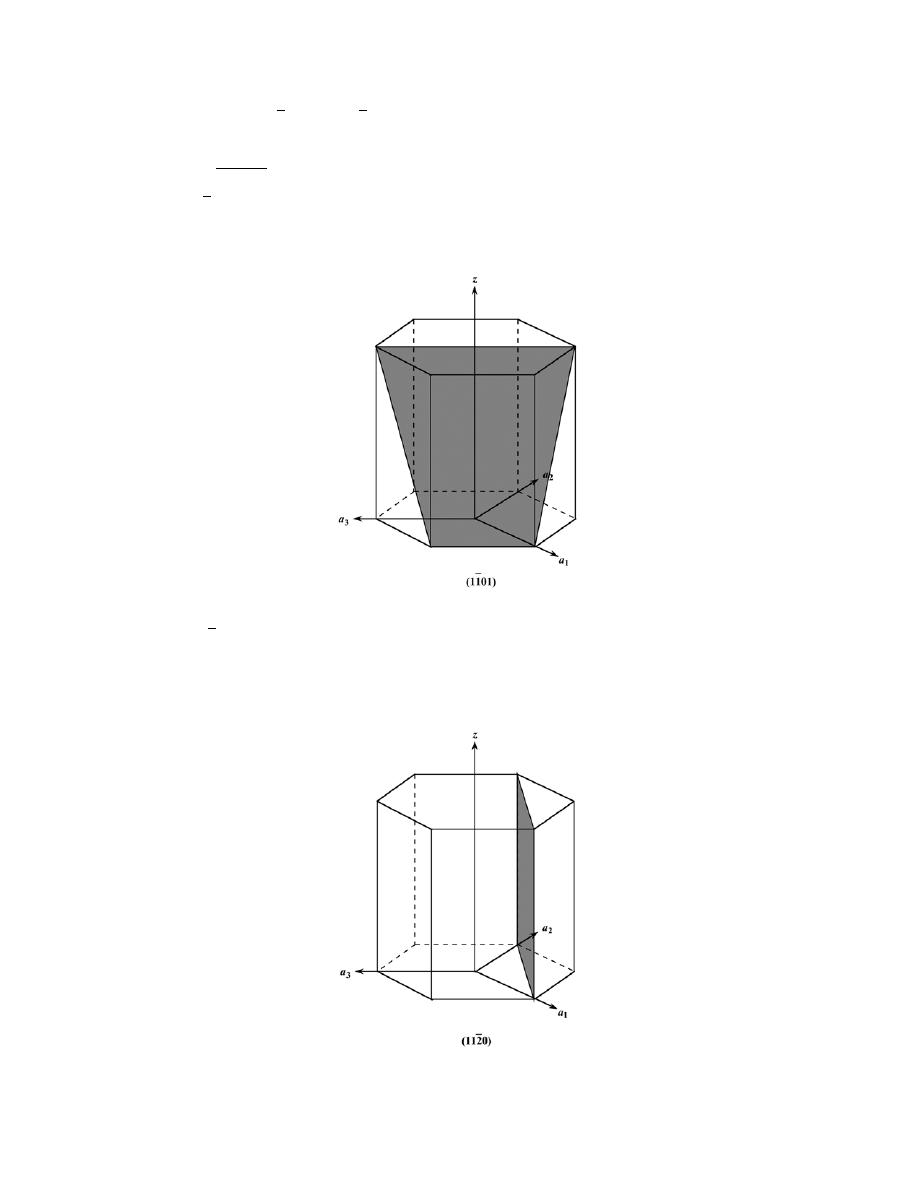
Excerpts from this work may be reproduced by instructors for distribution on a not-for-profit basis for testing or instructional purposes only to
students enrolled in courses for which the textbook has been adopted. Any other reproduction or translation of this work beyond that permitted
by Sections 107 or 108 of the 1976 United States Copyright Act without the permission of the copyright owner is unlawful.
3.51 Sketch the
(11 01) and
(112 0) planes in a hexagonal unit cell.
Solution
For
(1 1 01) the reciprocals of h, k, i, and l are, respectively, 1, –1,
∞, and 1; thus, this plane is parallel to
the a
3
axis, and intersects the a
1
axis at a, the a
2
axis at –a, and the z-axis at c. The plane having these intersections
is shown in the figure below
For
(112 0) the reciprocals of h, k, i, and l are, respectively, 1, 1, –1/2, and
∞; thus, this plane is parallel to
the z axis, and intersects the a
1
axis at a, the a
2
axis at a, and the a
3
axis at –a/2. The plane having these
intersections is shown in the figure below.
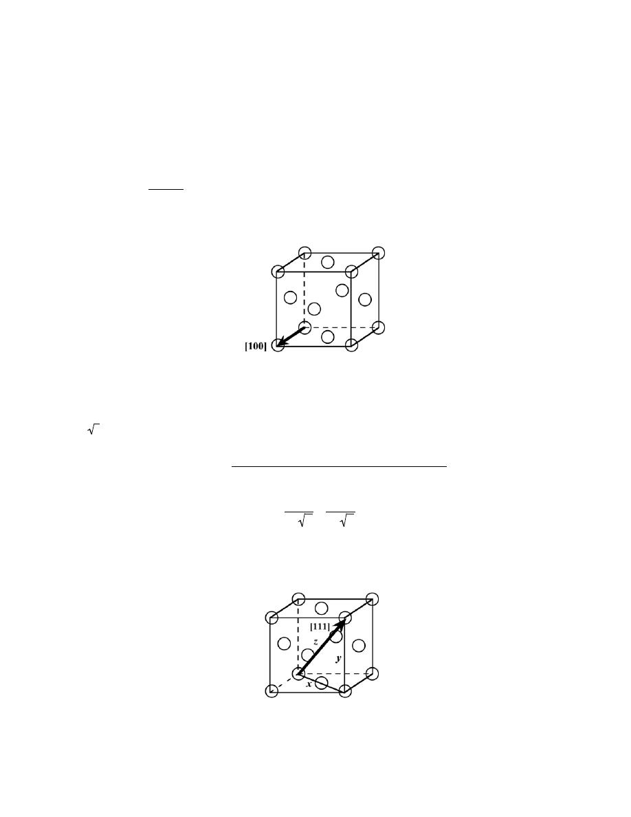
Excerpts from this work may be reproduced by instructors for distribution on a not-for-profit basis for testing or instructional purposes only to
students enrolled in courses for which the textbook has been adopted. Any other reproduction or translation of this work beyond that permitted
by Sections 107 or 108 of the 1976 United States Copyright Act without the permission of the copyright owner is unlawful.
Linear and Planar Densities
3.52 (a) Derive linear density expressions for FCC [100] and [111] directions in terms of the atomic
radius R.
(b) Compute and compare linear density values for these same two directions for silver.
Solution
(a) In the figure below is shown a [100] direction within an FCC unit cell.
For this [100] direction there is one atom at each of the two unit cell corners, and, thus, there is the equivalent of 1
atom that is centered on the direction vector. The length of this direction vector is just the unit cell edge length,
2R 2 (Equation 3.1). Therefore, the expression for the linear density of this plane is
LD
100
=
number of atoms centered on [100] direction vector
length of [100] direction vector
=
1 atom
2 R 2
=
1
2 R 2
An FCC unit cell within which is drawn a [111] direction is shown below.
Excerpts from this work may be reproduced by instructors for distribution on a not-for-profit basis for testing or instructional purposes only to
students enrolled in courses for which the textbook has been adopted. Any other reproduction or translation of this work beyond that permitted
by Sections 107 or 108 of the 1976 United States Copyright Act without the permission of the copyright owner is unlawful.
For this [111] direction, the vector shown passes through only the centers of the single atom at each of its ends, and,
thus, there is the equivalence of 1 atom that is centered on the direction vector. The length of this direction vector is
denoted by z in this figure, which is equal to
z
=
x
2
+ y
2
where x is the length of the bottom face diagonal, which is equal to 4R. Furthermore, y is the unit cell edge length,
which is equal to
2R 2 (Equation 3.1). Thus, using the above equation, the length z may be calculated as follows:
z
=
(
4R
)
2
+
(
2 R 2
)
2
= 24 R
2
= 2 R 6
Therefore, the expression for the linear density of this direction is
LD
111
=
number of atoms centered on [111] direction vector
length of [111] direction vector
=
1 atom
2 R 6
=
1
2 R 6
(b) From the table inside the front cover, the atomic radius for silver is 0.144 nm. Therefore, the linear
density for the [100] direction is
LD
100
(Ag)
=
1
2 R 2
=
1
(2)(0.144 nm)
2
= 2.46 nm
−1
= 2.46 × 10
9
m
−1
While for the [111] direction
LD
111
(Ag)
=
1
2 R 6
=
1
(2)(0.144 nm)
6
= 1.42 nm
−1
= 1.42 × 10
9
m
−1
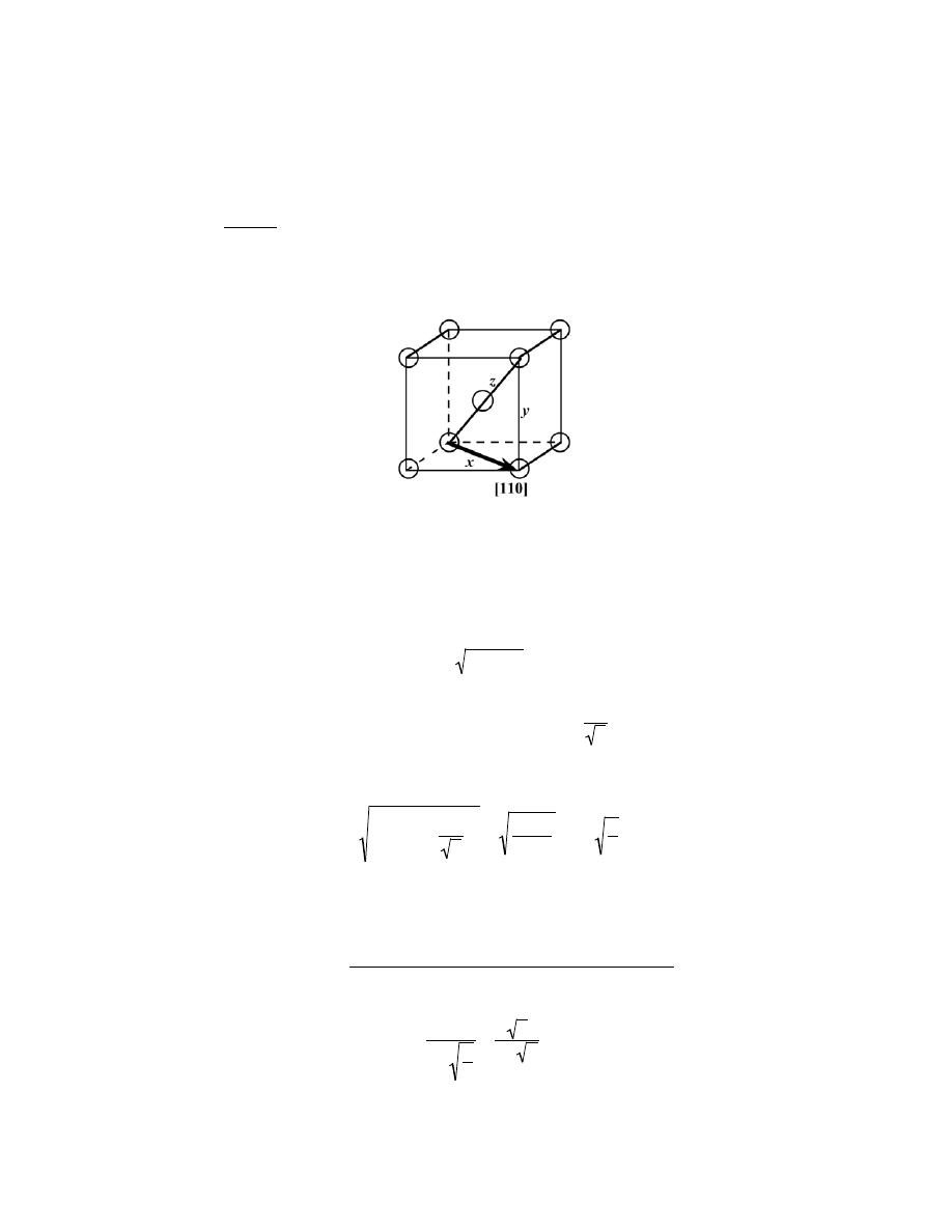
Excerpts from this work may be reproduced by instructors for distribution on a not-for-profit basis for testing or instructional purposes only to
students enrolled in courses for which the textbook has been adopted. Any other reproduction or translation of this work beyond that permitted
by Sections 107 or 108 of the 1976 United States Copyright Act without the permission of the copyright owner is unlawful.
3.53 (a) Derive linear density expressions for BCC [110] and [111] directions in terms of the atomic
radius R.
(b) Compute and compare linear density values for these same two directions for tungsten.
Solution
(a) In the figure below is shown a [110] direction within a BCC unit cell.
For this [110] direction there is one atom at each of the two unit cell corners, and, thus, there is the equivalence of 1
atom that is centered on the direction vector. The length of this direction vector is denoted by x in this figure, which
is equal to
x
=
z
2
− y
2
where y is the unit cell edge length, which, from Equation 3.3 is equal to
4 R
3
. Furthermore, z is the length of the
unit cell diagonal, which is equal to 4R Thus, using the above equation, the length x may be calculated as follows:
x
=
(
4R
)
2
−
4 R
3
2
=
32 R
2
3
= 4 R
2
3
Therefore, the expression for the linear density of this direction is
LD
110
=
number of atoms centered on [110] direction vector
length of [110] direction vector
=
1 atom
4 R
2
3
=
3
4 R 2
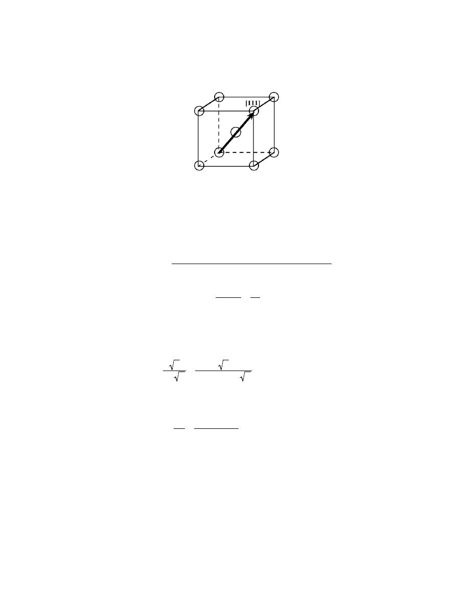
Excerpts from this work may be reproduced by instructors for distribution on a not-for-profit basis for testing or instructional purposes only to
students enrolled in courses for which the textbook has been adopted. Any other reproduction or translation of this work beyond that permitted
by Sections 107 or 108 of the 1976 United States Copyright Act without the permission of the copyright owner is unlawful.
A BCC unit cell within which is drawn a [111] direction is shown below.
For although the [111] direction vector shown passes through the centers of three atoms, there is an equivalence of
only two atoms associated with this unit cell—one-half of each of the two atoms at the end of the vector, in addition
to the center atom belongs entirely to the unit cell. Furthermore, the length of the vector shown is equal to 4R, since
all of the atoms whose centers the vector passes through touch one another. Therefore, the linear density is equal to
LD
111
=
number of atoms centered on [111] direction vector
length of [111] direction vector
=
2 atoms
4R
=
1
2R
(b) From the table inside the front cover, the atomic radius for tungsten is 0.137 nm. Therefore, the linear
density for the [110] direction is
LD
110
(W)
=
3
4 R 2
=
3
(4)(0.137 nm)
2
= 2.23 nm
−1
= 2.23 × 10
9
m
−1
While for the [111] direction
LD
111
(W)
=
1
2 R
=
1
(2)(0.137 nm)
= 3.65 nm
−1
= 3.65 × 10
9
m
−1
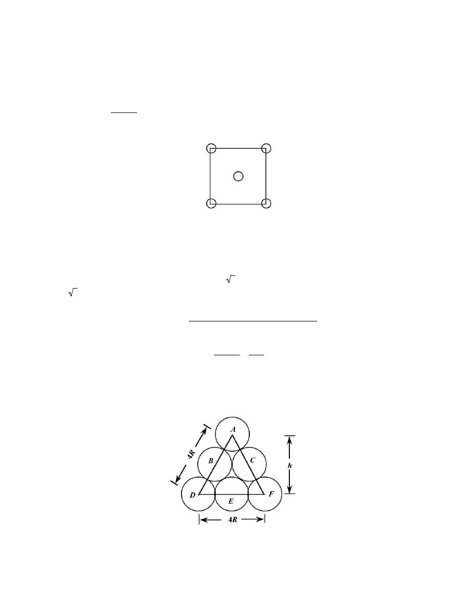
Excerpts from this work may be reproduced by instructors for distribution on a not-for-profit basis for testing or instructional purposes only to
students enrolled in courses for which the textbook has been adopted. Any other reproduction or translation of this work beyond that permitted
by Sections 107 or 108 of the 1976 United States Copyright Act without the permission of the copyright owner is unlawful.
3.54 (a) Derive planar density expressions for FCC (100) and (111) planes in terms of the atomic radius
R.
(b) Compute and compare planar density values for these same two planes for nickel.
Solution
(a) In the figure below is shown a (100) plane for an FCC unit cell.
For this (100) plane there is one atom at each of the four cube corners, each of which is shared with four adjacent
unit cells, while the center atom lies entirely within the unit cell. Thus, there is the equivalence of 2 atoms
associated with this FCC (100) plane. The planar section represented in the above figure is a square, wherein the
side lengths are equal to the unit cell edge length,
2R 2 (Equation 3.1); and, thus, the area of this square is just
(
2R 2
)
2
= 8R
2
. Hence, the planar density for this (100) plane is just
PD
100
=
number of atoms centered on (100) plane
area of (100) plane
=
2 atoms
8R
2
=
1
4R
2
That portion of an FCC (111) plane contained within a unit cell is shown below.
Excerpts from this work may be reproduced by instructors for distribution on a not-for-profit basis for testing or instructional purposes only to
students enrolled in courses for which the textbook has been adopted. Any other reproduction or translation of this work beyond that permitted
by Sections 107 or 108 of the 1976 United States Copyright Act without the permission of the copyright owner is unlawful.
There are six atoms whose centers lie on this plane, which are labeled A through F. One-sixth of each of atoms A,
D, and F are associated with this plane (yielding an equivalence of one-half atom), with one-half of each of atoms
B, C, and E (or an equivalence of one and one-half atoms) for a total equivalence of two atoms. Now, the area of
the triangle shown in the above figure is equal to one-half of the product of the base length and the height, h. If we
consider half of the triangle, then
(2 R)
2
+ h
2
= (4 R)
2
which leads to h =
2 R 3 . Thus, the area is equal to
Area
=
4 R(h)
2
=
(4 R)
(
2 R 3
)
2
= 4 R
2
3
And, thus, the planar density is
PD
111
=
number of atoms centered on (111) plane
area of (111) plane
=
2 atoms
4 R
2
3
=
1
2 R
2
3
(b) From the table inside the front cover, the atomic radius for nickel is 0.125 nm. Therefore, the planar
density for the (100) plane is
PD
100
(Ni)
=
1
4 R
2
=
1
4 (0.125 nm)
2
= 16.00 nm
−2
= 1.600 × 10
19
m
−2
While for the (111) plane
PD
111
(Ni)
=
1
2 R
2
3
=
1
2
3 (0.125 nm)
2
= 18.48 nm
−2
= 1.848 × 10
19
m
−2
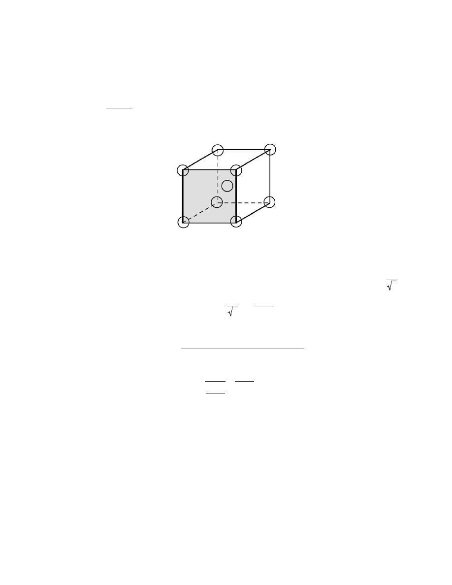
Excerpts from this work may be reproduced by instructors for distribution on a not-for-profit basis for testing or instructional purposes only to
students enrolled in courses for which the textbook has been adopted. Any other reproduction or translation of this work beyond that permitted
by Sections 107 or 108 of the 1976 United States Copyright Act without the permission of the copyright owner is unlawful.
3.55 (a) Derive planar density expressions for BCC (100) and (110) planes in terms of the atomic radius
R.
(b) Compute and compare planar density values for these same two planes for vanadium.
Solution
(a) A BCC unit cell within which is drawn a (100) plane is shown below.
For this (100) plane there is one atom at each of the four cube corners, each of which is shared with four adjacent
unit cells. Thus, there is the equivalence of 1 atom associated with this BCC (100) plane. The planar section
represented in the above figure is a square, wherein the side lengths are equal to the unit cell edge length,
4 R
3
(Equation 3.3); and, thus, the area of this square is just
4R
3
2
=
16 R
2
3
. Hence, the planar density for this (100)
plane is just
PD
100
=
number of atoms centered on (100) plane
area of (100) plane
=
1 atom
16 R
2
3
=
3
16 R
2
A BCC unit cell within which is drawn a (110) plane is shown below.
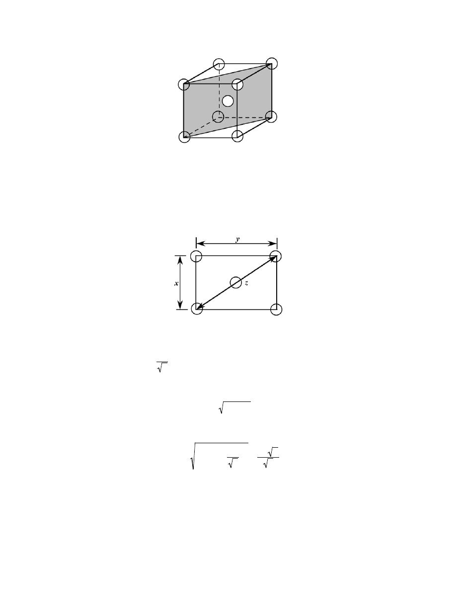
Excerpts from this work may be reproduced by instructors for distribution on a not-for-profit basis for testing or instructional purposes only to
students enrolled in courses for which the textbook has been adopted. Any other reproduction or translation of this work beyond that permitted
by Sections 107 or 108 of the 1976 United States Copyright Act without the permission of the copyright owner is unlawful.
For this (110) plane there is one atom at each of the four cube corners through which it passes, each of which is
shared with four adjacent unit cells, while the center atom lies entirely within the unit cell. Thus, there is the
equivalence of 2 atoms associated with this BCC (110) plane. The planar section represented in the above figure is
a rectangle, as noted in the figure below.
From this figure, the area of the rectangle is the product of x and y. The length x is just the unit cell edge length,
which for BCC (Equation 3.3) is
4 R
3
. Now, the diagonal length z is equal to 4R. For the triangle bounded by the
lengths x, y, and z
y
=
z
2
− x
2
Or
y
=
(4 R)
2
−
4R
3
2
=
4 R 2
3
Thus, in terms of R, the area of this (110) plane is just
Excerpts from this work may be reproduced by instructors for distribution on a not-for-profit basis for testing or instructional purposes only to
students enrolled in courses for which the textbook has been adopted. Any other reproduction or translation of this work beyond that permitted
by Sections 107 or 108 of the 1976 United States Copyright Act without the permission of the copyright owner is unlawful.
Area (110)
= xy =
4 R
3
4 R 2
3
=
16 R
2
2
3
And, finally, the planar density for this (110) plane is just
PD
110
=
number of atoms centered on (110) plane
area of (110) plane
=
2 atoms
16 R
2
2
3
=
3
8 R
2
2
(b) From the table inside the front cover, the atomic radius for vanadium is 0.132 nm. Therefore, the
planar density for the (100) plane is
PD
100
(V)
=
3
16 R
2
=
3
16 (0.132 nm)
2
= 10.76 nm
−2
= 1.076 × 10
19
m
−2
While for the (110) plane
PD
110
(V)
=
3
8 R
2
2
=
3
8 (0.132 nm)
2
2
= 15.22 nm
−2
= 1.522 × 10
19
m
−2
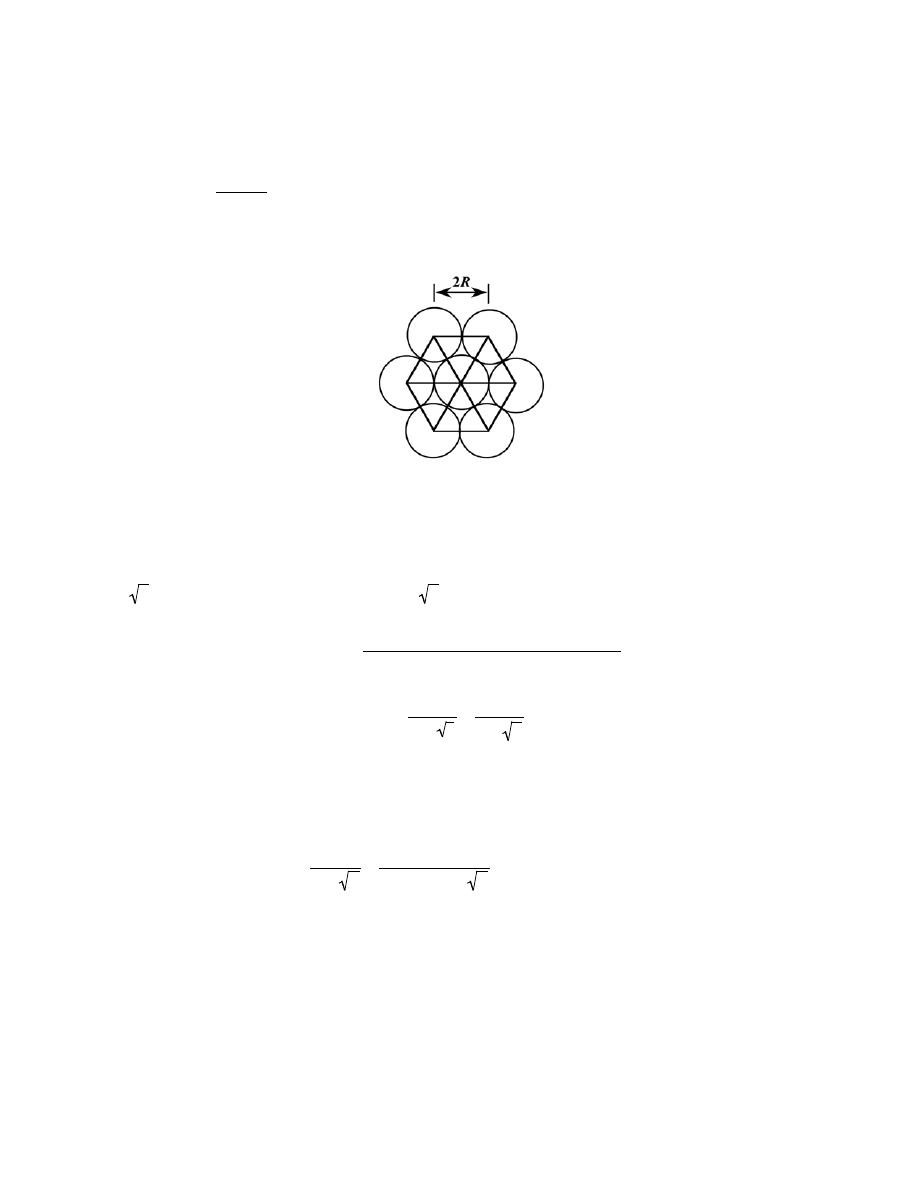
Excerpts from this work may be reproduced by instructors for distribution on a not-for-profit basis for testing or instructional purposes only to
students enrolled in courses for which the textbook has been adopted. Any other reproduction or translation of this work beyond that permitted
by Sections 107 or 108 of the 1976 United States Copyright Act without the permission of the copyright owner is unlawful.
3.56 (a) Derive the planar density expression for the HCP (0001) plane in terms of the atomic radius R.
(b) Compute the planar density value for this same plane for magnesium.
Solution
(a) A (0001) plane for an HCP unit cell is show below.
Each of the 6 perimeter atoms in this plane is shared with three other unit cells, whereas the center atom is shared
with no other unit cells; this gives rise to three equivalent atoms belonging to this plane.
In terms of the atomic radius R, the area of each of the 6 equilateral triangles that have been drawn is
R
2
3
, or the total area of the plane shown is
6 R
2
3
. And the planar density for this (0001) plane is equal to
PD
0001
=
number of atoms centered on (0001) plane
area of (0001) plane
=
3 atoms
6R
2
3
=
1
2R
2
3
(b) From the table inside the front cover, the atomic radius for magnesium is 0.160 nm. Therefore, the
planar density for the (0001) plane is
PD
0001
(Mg)
=
1
2 R
2
3
=
1
2 (0.160 nm)
2
3
= 11.28 nm
−2
= 1.128 × 10
19
m
−2

Excerpts from this work may be reproduced by instructors for distribution on a not-for-profit basis for testing or instructional purposes only to
students enrolled in courses for which the textbook has been adopted. Any other reproduction or translation of this work beyond that permitted
by Sections 107 or 108 of the 1976 United States Copyright Act without the permission of the copyright owner is unlawful.
Polycrystalline Materials
3.57 Explain why the properties of polycrystalline materials are most often isotropic.
Solution
Although each individual grain in a polycrystalline material may be anisotropic, if the grains have random
orientations, then the solid aggregate of the many anisotropic grains will behave isotropically.
Excerpts from this work may be reproduced by instructors for distribution on a not-for-profit basis for testing or instructional purposes only to
students enrolled in courses for which the textbook has been adopted. Any other reproduction or translation of this work beyond that permitted
by Sections 107 or 108 of the 1976 United States Copyright Act without the permission of the copyright owner is unlawful.
X-ray Diffraction: Determination of Crystal Structures
3.58 Using the data for molybdenum in Table 3.1, compute the interplanar spacing for the (111) set of
planes.
Solution
From the Table 3.1, molybdenum has a BCC crystal structure and an atomic radius of 0.1363 nm. Using
Equation (3.3), the lattice parameter a may be computed as
a
=
4 R
3
=
(4)(0.1363 nm)
3
= 0.3148 nm
Now, the interplanar spacing d
111
maybe determined using Equation 3.14 as
d
111
=
a
(1)
2
+ (1)
2
+ (1)
2
=
0.3148 nm
3
= 0.1817 nm
Excerpts from this work may be reproduced by instructors for distribution on a not-for-profit basis for testing or instructional purposes only to
students enrolled in courses for which the textbook has been adopted. Any other reproduction or translation of this work beyond that permitted
by Sections 107 or 108 of the 1976 United States Copyright Act without the permission of the copyright owner is unlawful.
3.59 Determine the expected diffraction angle for the first-order reflection from the (113) set of planes for
FCC platinum when monochromatic radiation of wavelength 0.1542 nm is used.
Solution
We first calculate the lattice parameter using Equation 3.1 and the value of R (0.1387 nm) cited in Table
3.1, as follows:
a = 2 R 2 = (2)(0.1387 nm)( 2) = 0.3923 nm
Next, the interplanar spacing for the (113) set of planes may be determined using Equation 3.14 according to
d
113
=
a
(1)
2
+ (1)
2
+ (3)
2
=
0.3923 nm
11
= 0.1183 nm
And finally, employment of Equation 3.13 yields the diffraction angle as
sin
θ =
n
λ
2d
113
=
(1)(0.1542 nm)
(2)(0.1183 nm)
= 0.652
Which leads to
θ = sin
-1
(0.652) = 40.69
°
And, finally
2
θ = (2)(40.69°) = 81.38°
Excerpts from this work may be reproduced by instructors for distribution on a not-for-profit basis for testing or instructional purposes only to
students enrolled in courses for which the textbook has been adopted. Any other reproduction or translation of this work beyond that permitted
by Sections 107 or 108 of the 1976 United States Copyright Act without the permission of the copyright owner is unlawful.
3.60 Using the data for aluminum in Table 3.1, compute the interplanar spacings for the (110) and (221)
sets of planes.
Solution
From the table, aluminum has an FCC crystal structure and an atomic radius of 0.1431 nm. Using
Equation 3.1 the lattice parameter, a, may be computed as
a = 2R 2 = (2) (0.1431 nm)( 2) = 0.4047 nm
Now, the d
110
interplanar spacing may be determined using Equation 3.14 as
d
110
=
a
(1)
2
+ (1)
2
+ (0)
2
=
0.4047 nm
2
= 0.2862 nm
And, similarly for d
221
d
221
=
a
(2)
2
+ (2)
2
+ (1)
2
=
0.4047 nm
9
= 0.1349 nm
Excerpts from this work may be reproduced by instructors for distribution on a not-for-profit basis for testing or instructional purposes only to
students enrolled in courses for which the textbook has been adopted. Any other reproduction or translation of this work beyond that permitted
by Sections 107 or 108 of the 1976 United States Copyright Act without the permission of the copyright owner is unlawful.
3.61 The metal iridium has an FCC crystal structure. If the angle of diffraction for the (220) set of planes
occurs at 69.22
° (first-order reflection) when monochromatic x-radiation having a wavelength of 0.1542 nm is
used, compute (a) the interplanar spacing for this set of planes, and (b) the atomic radius for an iridium atom.
Solution
(a) From the data given in the problem, and realizing that 69.22
° = 2θ, the interplanar spacing for the
(220) set of planes for iridium may be computed using Equation 3.13 as
d
220
=
n
λ
2 sin
θ
=
(1)(0.1542 nm)
(2) sin
69.22
°
2
= 0.1357 nm
(b) In order to compute the atomic radius we must first determine the lattice parameter, a, using Equation
3.14, and then R from Equation 3.1 since Ir has an FCC crystal structure. Therefore,
a = d
220
(2)
2
+ (2)
2
+ (0)
2
= (0.1357 nm)
(
8
)
= 0.3838 nm
And, from Equation 3.1
R =
a
2 2
=
0.3838 nm
2 2
= 0.1357 nm
Excerpts from this work may be reproduced by instructors for distribution on a not-for-profit basis for testing or instructional purposes only to
students enrolled in courses for which the textbook has been adopted. Any other reproduction or translation of this work beyond that permitted
by Sections 107 or 108 of the 1976 United States Copyright Act without the permission of the copyright owner is unlawful.
3.62 The metal rubidium has a BCC crystal structure. If the angle of diffraction for the (321) set of planes
occurs at 27.00
° (first-order reflection) when monochromatic x-radiation having a wavelength of 0.0711 nm is
used, compute (a) the interplanar spacing for this set of planes, and (b) the atomic radius for the rubidium atom.
Solution
(a) From the data given in the problem, and realizing that 27.00
° = 2θ, the interplanar spacing for the
(321) set of planes for Rb may be computed using Equation 3.13 as follows:
d
321
=
n
λ
2 sin
θ
=
(1)(0.0711 nm)
(2) sin
27.00
°
2
= 0.1523 nm
(b) In order to compute the atomic radius we must first determine the lattice parameter, a, using Equation
3.14, and then R from Equation 3.3 since Rb has a BCC crystal structure. Therefore,
a = d
321
(3)
2
+ (2)
2
+ (1)
2
= (0.1523 nm)
(
14
)
= 0.5700 nm
And, from Equation 3.3
R
=
a 3
4
=
(0.5700 nm)
3
4
= 0.2468 nm
Excerpts from this work may be reproduced by instructors for distribution on a not-for-profit basis for testing or instructional purposes only to
students enrolled in courses for which the textbook has been adopted. Any other reproduction or translation of this work beyond that permitted
by Sections 107 or 108 of the 1976 United States Copyright Act without the permission of the copyright owner is unlawful.
3.63 For which set of crystallographic planes will a first-order diffraction peak occur at a diffraction
angle of 46.21
° for BCC iron when monochromatic radiation having a wavelength of 0.0711 nm is used?
Solution
The first step to solve this problem is to compute the interplanar spacing using Equation 3.13. Thus,
d
hkl
=
n
λ
2 sin
θ
=
(1)(0.0711 nm)
(2) sin
46.21
°
2
= 0.0906 nm
Now, employment of both Equations 3.14 and 3.3 (since Fe’s crystal structure is BCC), and the value of R for iron
from Table 3.1 (0.1241 nm) leads to
h
2
+ k
2
+ l
2
=
a
d
hkl
=
4R
d
hkl
3
=
(4)(0.1241 nm)
(0.0906 nm)( 3)
= 3.163
This means that
h
2
+ k
2
+ l
2
= (3.163)
2
= 10.0
By trial and error, the only three integers having a sum that is even, and the sum of the squares of which equals 10.0
are 3, 1, and 0. Therefore, the set of planes responsible for this diffraction peak are the (310) ones.
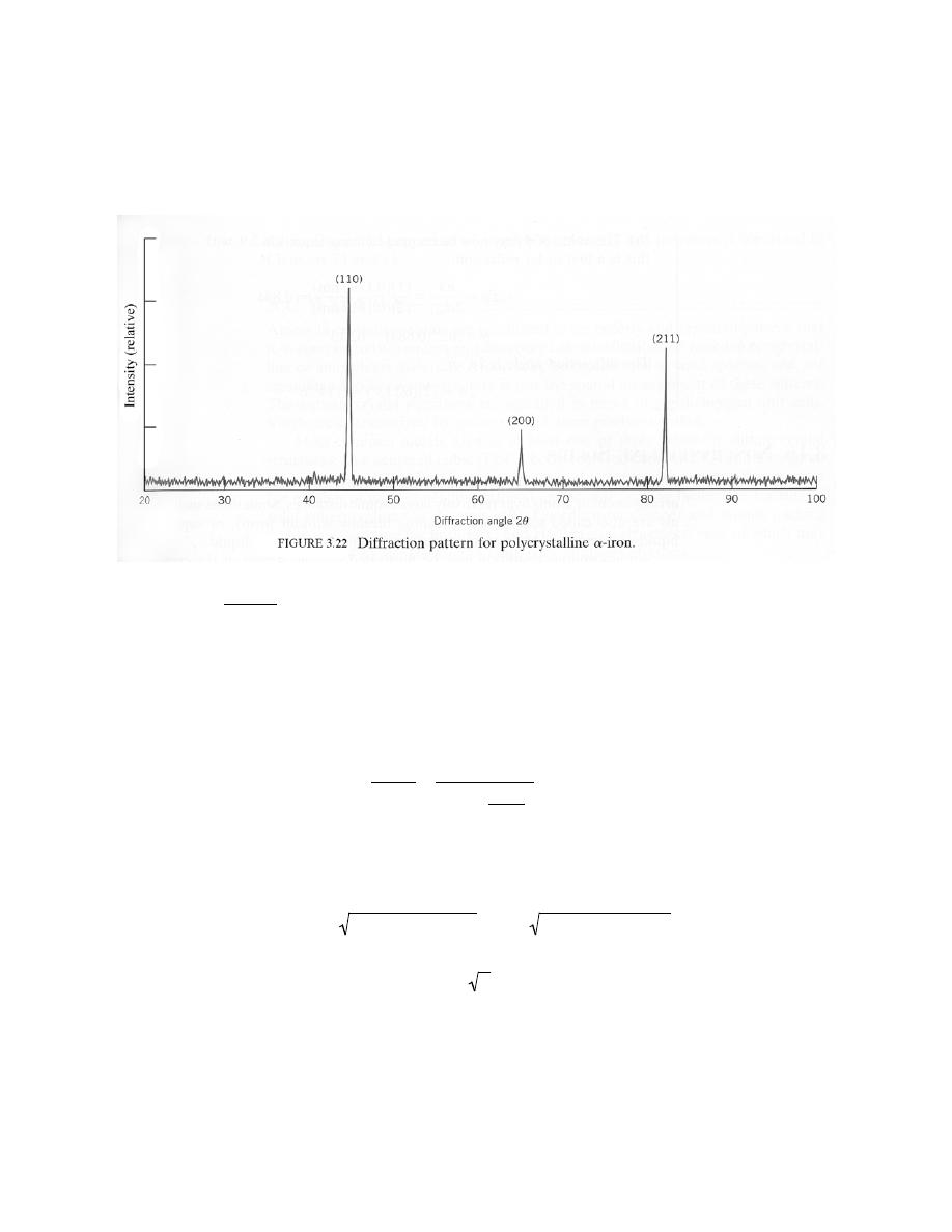
Excerpts from this work may be reproduced by instructors for distribution on a not-for-profit basis for testing or instructional purposes only to
students enrolled in courses for which the textbook has been adopted. Any other reproduction or translation of this work beyond that permitted
by Sections 107 or 108 of the 1976 United States Copyright Act without the permission of the copyright owner is unlawful.
3.64 Figure 3.22 shows an x-ray diffraction pattern for
α-iron taken using a diffractometer and
monochromatic x-radiation having a wavelength of 0.1542 nm; each diffraction peak on the pattern has been
indexed. Compute the interplanar spacing for each set of planes indexed; also determine the lattice parameter of Fe
for each of the peaks.
Solution
For each peak, in order to compute the interplanar spacing and the lattice parameter we must employ
Equations 3.14 and 3.13, respectively. The first peak of Figure 3.22, which results from diffraction by the (110) set
of planes, occurs at
2θ = 45.0°; the corresponding interplanar spacing for this set of planes, using Equation 3.13, is
equal to
d
110
=
n
λ
2 sin
θ
=
(1)(0.1542 nm)
(2) sin
45.0
°
2
= 0.2015 nm
And, from Equation 3.14, the lattice parameter a is determined as
a = d
hkl
(h)
2
+ (k)
2
+ (l)
2
= d
110
(1)
2
+ (1)
2
+ (0)
2
= (0.2015 nm)
2 = 0.2850 nm
Similar computations are made for the other peaks which results are tabulated below:

Excerpts from this work may be reproduced by instructors for distribution on a not-for-profit basis for testing or instructional purposes only to
students enrolled in courses for which the textbook has been adopted. Any other reproduction or translation of this work beyond that permitted
by Sections 107 or 108 of the 1976 United States Copyright Act without the permission of the copyright owner is unlawful.
Peak Index
2
θ
d
hkl
(nm)
a (nm)
200
65.1
0.1433
0.2866
211
82.8
0.1166
0.2856

Excerpts from this work may be reproduced by instructors for distribution on a not-for-profit basis for testing or instructional purposes only to
students enrolled in courses for which the textbook has been adopted. Any other reproduction or translation of this work beyond that permitted
by Sections 107 or 108 of the 1976 United States Copyright Act without the permission of the copyright owner is unlawful.
3.65 The diffraction peaks shown in Figure 3.22 are indexed according to the reflection rules for BCC
(i.e., the sum h + k + l must be even). Cite the h, k, and l indices for the first four diffraction peaks for FCC crystals
consistent with h, k, and l all being either odd or even.
Solution
The first four diffraction peaks that will occur for FCC consistent with h, k, and l all being odd or even are
(111), (200), (220), and (311).
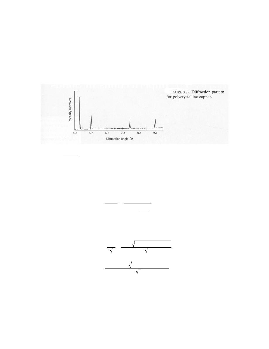
Excerpts from this work may be reproduced by instructors for distribution on a not-for-profit basis for testing or instructional purposes only to
students enrolled in courses for which the textbook has been adopted. Any other reproduction or translation of this work beyond that permitted
by Sections 107 or 108 of the 1976 United States Copyright Act without the permission of the copyright owner is unlawful.
3.66 Figure 3.25 shows the first four peaks of the x-ray diffraction pattern for copper, which has an FCC
crystal structure; monochromatic x-radiation having a wavelength of 0.1542 nm was used.
(a) Index (i.e., give h, k, and l indices) for each of these peaks.
(b) Determine the interplanar spacing for each of the peaks.
(c) For each peak, determine the atomic radius for Cu and compare these with the value presented in
Table 3.1.
Solution
(a) Since Cu has an FCC crystal structure, only those peaks for which h, k, and l are all either odd or even
will appear. Therefore, the first peak results by diffraction from (111) planes.
(b) For each peak, in order to calculate the interplanar spacing we must employ Equation 3.13. For the
first peak which occurs at 43.8
°
d
111
=
n
λ
2 sin
θ
=
(1)(0.1542 nm)
(2) sin
43.8
°
2
= 0.2067 nm
(c) Employment of Equations 3.14 and 3.1 is necessary for the computation of R for Cu as
R =
a
2 2
=
(
d
hkl
)
(h)
2
+ (k)
2
+ (l)
2
2 2
=
(
0.2067 nm
)
(1)
2
+ (1)
2
+ (1)
2
2 2
= 0.1266 nm
Similar computations are made for the other peaks which results are tabulated below:

Excerpts from this work may be reproduced by instructors for distribution on a not-for-profit basis for testing or instructional purposes only to
students enrolled in courses for which the textbook has been adopted. Any other reproduction or translation of this work beyond that permitted
by Sections 107 or 108 of the 1976 United States Copyright Act without the permission of the copyright owner is unlawful.
Peak Index
2
θ
d
hkl
(nm)
R (nm)
200
50.8
0.1797
0.1271
220
74.4
0.1275
0.1275
311
90.4
0.1087
0.1274

Excerpts from this work may be reproduced by instructors for distribution on a not-for-profit basis for testing or instructional purposes only to
students enrolled in courses for which the textbook has been adopted. Any other reproduction or translation of this work beyond that permitted
by Sections 107 or 108 of the 1976 United States Copyright Act without the permission of the copyright owner is unlawful.
Noncrystalline Solids
3.67 Would you expect a material in which the atomic bonding is predominantly ionic in nature to be
more or less likely to form a noncrystalline solid upon solidification than a covalent material? Why? (See Section
2.6.)
Solution
A material in which atomic bonding is predominantly ionic in nature is less likely to form a noncrystalline
solid upon solidification than a covalent material because covalent bonds are directional whereas ionic bonds are
nondirectional; it is more difficult for the atoms in a covalent material to assume positions giving rise to an ordered
structure.

Excerpts from this work may be reproduced by instructors for distribution on a not-for-profit basis for testing or instructional purposes only to
students enrolled in courses for which the textbook has been adopted. Any other reproduction or translation of this work beyond that permitted
by Sections 107 or 108 of the 1976 United States Copyright Act without the permission of the copyright owner is unlawful.
CHAPTER 4
IMPERFECTIONS IN SOLIDS
PROBLEM SOLUTIONS
Vacancies and Self-Interstitials
4.1 Calculate the fraction of atom sites that are vacant for lead at its melting temperature of 327°C (600
K). Assume an energy for vacancy formation of 0.55 eV/atom.
Solution
In order to compute the fraction of atom sites that are vacant in lead at 600 K, we must employ Equation
4.1. As stated in the problem, Q
v
= 0.55 eV/atom. Thus,
N
v
N
= exp
−
Q
v
kT
= exp −
0.55 eV / atom
(
8.62
× 10
−5
eV / atom - K
)
(600 K)
= 2.41
× 10
-5

Excerpts from this work may be reproduced by instructors for distribution on a not-for-profit basis for testing or instructional purposes only to
students enrolled in courses for which the textbook has been adopted. Any other reproduction or translation of this work beyond that permitted
by Sections 107 or 108 of the 1976 United States Copyright Act without the permission of the copyright owner is unlawful.
4.2 Calculate the number of vacancies per cubic meter in iron at 850
°C. The energy for vacancy
formation is 1.08 eV/atom. Furthermore, the density and atomic weight for Fe are 7.65 g/cm
3
and 55.85 g/mol,
respectively.
Solution
Determination of the number of vacancies per cubic meter in iron at 850
°C (1123 K) requires the
utilization of Equations 4.1 and 4.2 as follows:
N
v
= N exp
−
Q
v
kT
=
N
A
ρ
Fe
A
Fe
exp
−
Q
v
kT
And incorporation of values of the parameters provided in the problem statement into the above equation leads to
N
v
=
(
6.022
× 10
23
atoms / mol
)(
7.65 g / cm
3
)
55.85 g / mol
exp
−
1.08 eV / atom
(
8.62
× 10
−5
eV / atom
− K
)
(850
°C + 273 K)
= 1.18
× 10
18
cm
-3
= 1.18
× 10
24
m
-3
Excerpts from this work may be reproduced by instructors for distribution on a not-for-profit basis for testing or instructional purposes only to
students enrolled in courses for which the textbook has been adopted. Any other reproduction or translation of this work beyond that permitted
by Sections 107 or 108 of the 1976 United States Copyright Act without the permission of the copyright owner is unlawful.
4.3 Calculate the activation energy for vacancy formation in aluminum, given that the equilibrium number
of vacancies at 500
°C (773 K) is 7.57 × 10
23
m
-3
. The atomic weight and density (at 500
°C) for aluminum are,
respectively, 26.98 g/mol and 2.62 g/cm
3
.
Solution
Upon examination of Equation 4.1, all parameters besides Q
v
are given except N, the total number of
atomic sites. However, N is related to the density, (
ρ
Al
), Avogadro's number (N
A
), and the atomic weight (A
Al
)
according to Equation 4.2 as
N =
N
A
ρ
Al
A
Al
=
(
6.022
× 10
23
atoms / mol
)(
2.62 g / cm
3
)
26.98 g / mol
= 5.85
× 10
22
atoms/cm
3
= 5.85
× 10
28
atoms/m
3
Now, taking natural logarithms of both sides of Equation 4.1,
ln N
v
= ln N
−
Q
v
kT
and, after some algebraic manipulation
Q
v
=
− kT ln
N
v
N
=
−
(
8.62
× 10
-5
eV/atom - K
)
(500
°C + 273 K) ln
7.57
× 10
23
m
−3
5.85
× 10
28
m
−3
= 0.75 eV/atom

Excerpts from this work may be reproduced by instructors for distribution on a not-for-profit basis for testing or instructional purposes only to
students enrolled in courses for which the textbook has been adopted. Any other reproduction or translation of this work beyond that permitted
by Sections 107 or 108 of the 1976 United States Copyright Act without the permission of the copyright owner is unlawful.
Impurities in Solids
4.4 Below, atomic radius, crystal structure, electronegativity, and the most common valence are tabulated,
for several elements; for those that are nonmetals, only atomic radii are indicated.
Element
Atomic Radius
(nm)
Crystal Structure
Electronegativity
Valence
Cu
0.1278
FCC
1.9
+2
C
0.071
H
0.046
O
0.060
Ag
0.1445
FCC
1.9
+1
Al
0.1431
FCC
1.5
+3
Co
0.1253
HCP
1.8
+2
Cr
0.1249
BCC
1.6
+3
Fe
0.1241
BCC
1.8
+2
Ni
0.1246
FCC
1.8
+2
Pd
0.1376
FCC
2.2
+2
Pt
0.1387
FCC
2.2
+2
Zn
0.1332
HCP
1.6
+2
Which of these elements would you expect to form the following with copper:
(a) A substitutional solid solution having complete solubility
(b) A substitutional solid solution of incomplete solubility
(c) An interstitial solid solution
Solution
In this problem we are asked to cite which of the elements listed form with Cu the three possible solid
solution types. For complete substitutional solubility the following criteria must be met: 1) the difference in atomic
radii between Cu and the other element (
∆R%) must be less than ±15%, 2) the crystal structures must be the same,
3) the electronegativities must be similar, and 4) the valences should be the same, or nearly the same. Below are
tabulated, for the various elements, these criteria.
Crystal
∆Electro-
Element
∆R%
Structure
negativity
Valence
Cu
FCC
2+
C
–44

Excerpts from this work may be reproduced by instructors for distribution on a not-for-profit basis for testing or instructional purposes only to
students enrolled in courses for which the textbook has been adopted. Any other reproduction or translation of this work beyond that permitted
by Sections 107 or 108 of the 1976 United States Copyright Act without the permission of the copyright owner is unlawful.
H
–64
O
–53
Ag
+13
FCC
0
1+
Al
+12
FCC
-0.4
3+
Co
-2
HCP
-0.1
2+
Cr
-2
BCC
-0.3
3+
Fe
-3
BCC
-0.1
2+
Ni
-3
FCC
-0.1
2+
Pd
+8
FCC
+0.3
2+
Pt
+9
FCC
+0.3
2+
Zn
+4
HCP
-0.3
2+
(a) Ni, Pd, and Pt meet all of the criteria and thus form substitutional solid solutions having complete
solubility. At elevated temperatures Co and Fe experience allotropic transformations to the FCC crystal structure,
and thus display complete solid solubility at these temperatures.
(b) Ag, Al, Co, Cr, Fe, and Zn form substitutional solid solutions of incomplete solubility. All these metals
have either BCC or HCP crystal structures, and/or the difference between their atomic radii and that for Cu are
greater than ±15%, and/or have a valence different than 2+.
(c) C, H, and O form interstitial solid solutions. These elements have atomic radii that are significantly
smaller than the atomic radius of Cu.
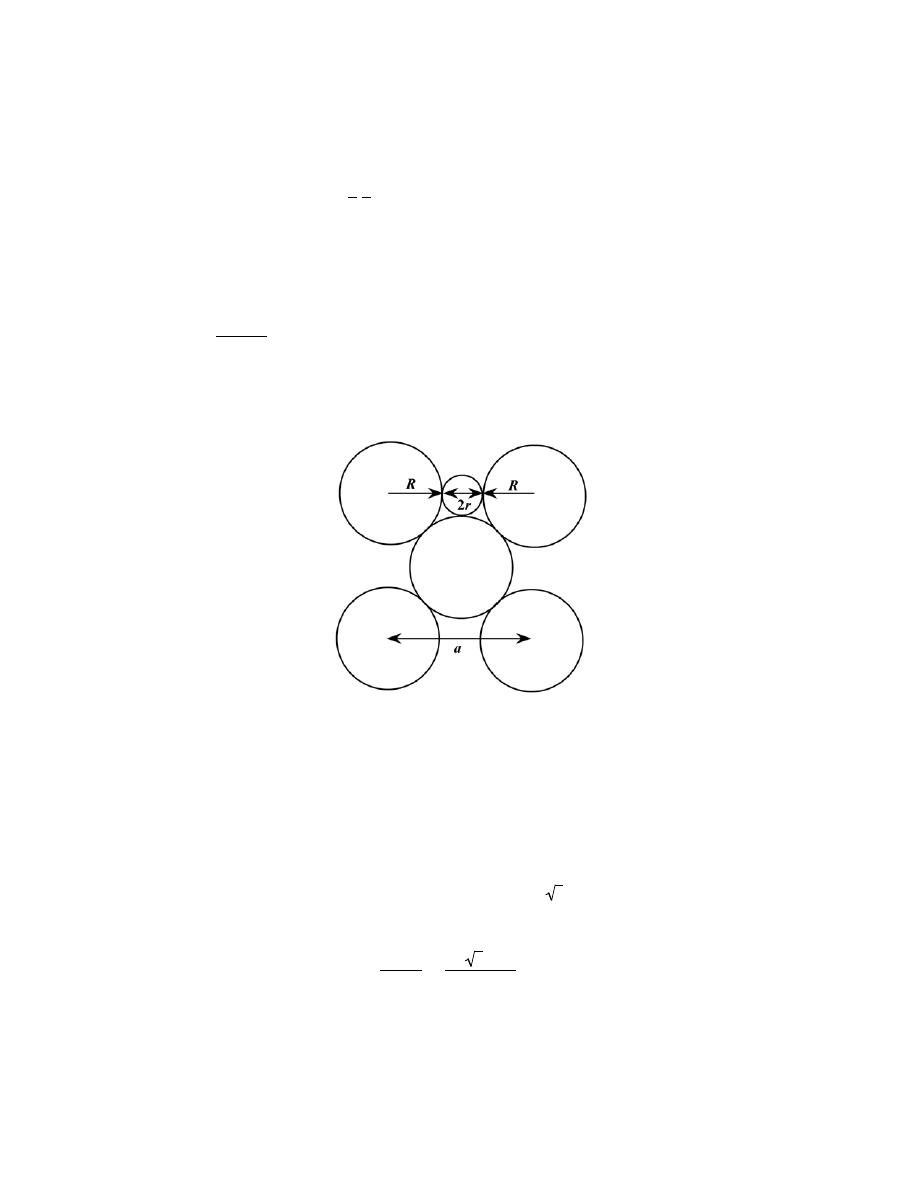
Excerpts from this work may be reproduced by instructors for distribution on a not-for-profit basis for testing or instructional purposes only to
students enrolled in courses for which the textbook has been adopted. Any other reproduction or translation of this work beyond that permitted
by Sections 107 or 108 of the 1976 United States Copyright Act without the permission of the copyright owner is unlawful.
4.5 For both FCC and BCC crystal structures, there are two different types of interstitial sites. In each
case, one site is larger than the other, and is normally occupied by impurity atoms. For FCC, this larger one is
located at the center of each edge of the unit cell; it is termed an octahedral interstitial site. On the other hand, with
BCC the larger site type is found at 0
1
2
1
4
positions—that is, lying on {100} faces, and situated midway between
two unit cell edges on this face and one-quarter of the distance between the other two unit cell edges; it is termed a
tetrahedral interstitial site. For both FCC and BCC crystal structures, compute the radius r of an impurity atom
that will just fit into one of these sites in terms of the atomic radius R of the host atom.
Solution
In the drawing below is shown the atoms on the (100) face of an FCC unit cell; the interstitial site is at the
center of the edge.
The diameter of an atom that will just fit into this site (2r) is just the difference between that unit cell edge length
(a) and the radii of the two host atoms that are located on either side of the site (R); that is
2r = a – 2R
However, for FCC a is related to R according to Equation 3.1 as
a
= 2R 2 ; therefore, solving for r from the above
equation gives
r =
a
− 2 R
2
=
2 R 2
− 2 R
2
= 0.41R
A (100) face of a BCC unit cell is shown below.
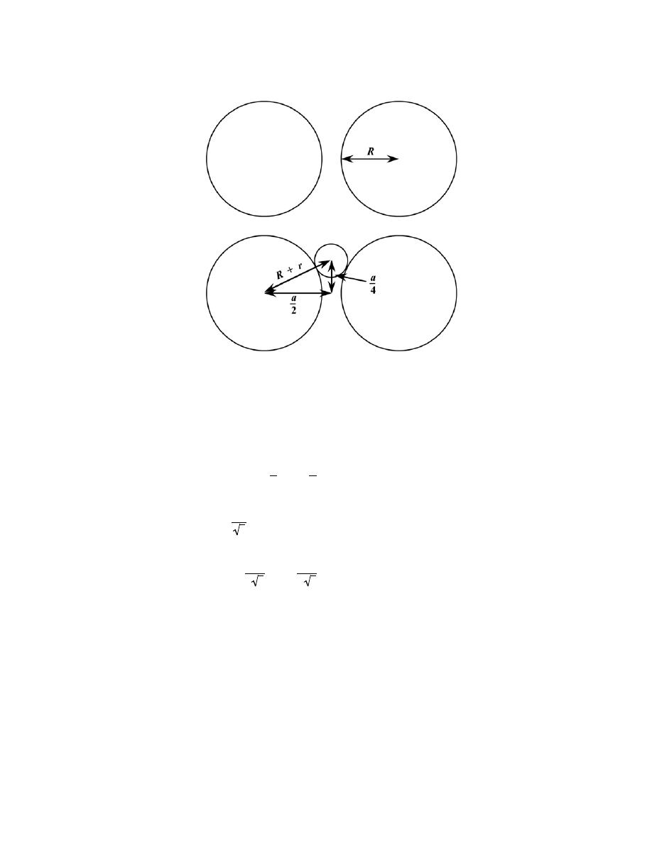
Excerpts from this work may be reproduced by instructors for distribution on a not-for-profit basis for testing or instructional purposes only to
students enrolled in courses for which the textbook has been adopted. Any other reproduction or translation of this work beyond that permitted
by Sections 107 or 108 of the 1976 United States Copyright Act without the permission of the copyright owner is unlawful.
The interstitial atom that just fits into this interstitial site is shown by the small circle. It is situated in the plane of
this (100) face, midway between the two vertical unit cell edges, and one quarter of the distance between the bottom
and top cell edges. From the right triangle that is defined by the three arrows we may write
a
2
2
+
a
4
2
=
(
R
+ r
)
2
However, from Equation 3.3,
a =
4R
3
, and, therefore, making this substitution, the above equation takes the form
4R
2 3
2
+
4R
4 3
2
= R
2
+ 2Rr + r
2
After rearrangement the following quadratic equation results:
r
2
+ 2Rr
− 0.667R
2
= 0
And upon solving for r:

Excerpts from this work may be reproduced by instructors for distribution on a not-for-profit basis for testing or instructional purposes only to
students enrolled in courses for which the textbook has been adopted. Any other reproduction or translation of this work beyond that permitted
by Sections 107 or 108 of the 1976 United States Copyright Act without the permission of the copyright owner is unlawful.
r
=
−(2R) ± (2R)
2
− (4)(1)(−0.667R
2
)
2
=
−2R ± 2.582R
2
And, finally
r(
+) =
−2R + 2.582R
2
= 0.291R
r(
−) =
−2R − 2.582R
2
= − 2.291R
Of course, only the r(+) root is possible, and, therefore, r = 0.291R.
Thus, for a host atom of radius R, the size of an interstitial site for FCC is approximately 1.4 times that for
BCC.

Excerpts from this work may be reproduced by instructors for distribution on a not-for-profit basis for testing or instructional purposes only to
students enrolled in courses for which the textbook has been adopted. Any other reproduction or translation of this work beyond that permitted
by Sections 107 or 108 of the 1976 United States Copyright Act without the permission of the copyright owner is unlawful.
Specification of Composition
4.6 Derive the following equations:
(a) Equation 4.7a
(b) Equation 4.9a
(c) Equation 4.10a
(d) Equation 4.11b
Solution
(a) This problem asks that we derive Equation 4.7a. To begin, C
1
is defined according to Equation 4.3 as
C
1
=
m
1
m
1
+ m
2
× 100
or, equivalently
C
1
=
m
1
'
m
1
'
+ m
2
'
× 100
where the primed m's indicate masses in grams. From Equation 4.4 we may write
m
1
'
= n
m1
A
1
m
2
'
= n
m2
A
2
And, substitution into the C
1
expression above
C
1
=
n
m1
A
1
n
m1
A
1
+ n
m2
A
2
× 100
From Equation 4.5 it is the case that
n
m1
=
C
1
'
(
n
m1
+ n
m2
)
100

Excerpts from this work may be reproduced by instructors for distribution on a not-for-profit basis for testing or instructional purposes only to
students enrolled in courses for which the textbook has been adopted. Any other reproduction or translation of this work beyond that permitted
by Sections 107 or 108 of the 1976 United States Copyright Act without the permission of the copyright owner is unlawful.
n
m2
=
C
2
'
(
n
m1
+ n
m2
)
100
And substitution of these expressions into the above equation leads to
C
1
=
C
1
'
A
1
C
1
'
A
1
+ C
2
'
A
2
× 100
which is just Equation 4.7a.
(b) This problem asks that we derive Equation 4.9a. To begin,
C
1
"
is defined as the mass of component 1
per unit volume of alloy, or
C
1
"
=
m
1
V
If we assume that the total alloy volume V is equal to the sum of the volumes of the two constituents--i.e., V = V
1
+
V
2
--then
C
1
"
=
m
1
V
1
+ V
2
Furthermore, the volume of each constituent is related to its density and mass as
V
1
=
m
1
ρ
1
V
2
=
m
2
ρ
2
This leads to
C
1
"
=
m
1
m
1
ρ
1
+
m
2
ρ
2
From Equation 4.3, m
1
and m
2
may be expressed as follows:

Excerpts from this work may be reproduced by instructors for distribution on a not-for-profit basis for testing or instructional purposes only to
students enrolled in courses for which the textbook has been adopted. Any other reproduction or translation of this work beyond that permitted
by Sections 107 or 108 of the 1976 United States Copyright Act without the permission of the copyright owner is unlawful.
m
1
=
C
1
(
m
1
+ m
2
)
100
m
2
=
C
2
(
m
1
+ m
2
)
100
Substitution of these equations into the preceding expression yields
C
1
"
=
C
1
(
m
1
+ m
2
)
100
C
1
(
m
1
+ m
2
)
100
ρ
1
+
C
2
(
m
1
+ m
2
)
100
ρ
2
=
C
1
C
1
ρ
1
+
C
2
ρ
2
If the densities
ρ
1
and
ρ
2
are given in units of g/cm
3
, then conversion to units of kg/m
3
requires that we multiply
this equation by 10
3
, inasmuch as
1 g/cm
3
= 10
3
kg/m
3
Therefore, the previous equation takes the form
C
1
"
=
C
1
C
1
ρ
1
+
C
2
ρ
2
× 10
3
which is the desired expression.
(c) Now we are asked to derive Equation 4.10a. The density of an alloy
ρ
ave
is just the total alloy mass M
divided by its volume V
ρ
ave
=
M
V

Excerpts from this work may be reproduced by instructors for distribution on a not-for-profit basis for testing or instructional purposes only to
students enrolled in courses for which the textbook has been adopted. Any other reproduction or translation of this work beyond that permitted
by Sections 107 or 108 of the 1976 United States Copyright Act without the permission of the copyright owner is unlawful.
Or, in terms of the component elements 1 and 2
ρ
ave
=
m
1
+ m
2
V
1
+ V
2
[Note: here it is assumed that the total alloy volume is equal to the separate volumes of the individual components,
which is only an approximation; normally V will not be exactly equal to (V
1
+ V
2
)].
Each of V
1
and V
2
may be expressed in terms of its mass and density as,
V
1
=
m
1
ρ
1
V
2
=
m
2
ρ
2
When these expressions are substituted into the above equation, we get
ρ
ave
=
m
1
+ m
2
m
1
ρ
1
+
m
2
ρ
2
Furthermore, from Equation 4.3
m
1
=
C
1
(
m
1
+ m
2
)
100
m
2
=
C
2
(
m
1
+ m
2
)
100
Which, when substituted into the above
ρ
ave
expression yields
ρ
ave
=
m
1
+ m
2
C
1
(
m
1
+ m
2
)
100
ρ
1
+
C
2
(
m
1
+ m
2
)
100
ρ
2
And, finally, this equation reduces to

Excerpts from this work may be reproduced by instructors for distribution on a not-for-profit basis for testing or instructional purposes only to
students enrolled in courses for which the textbook has been adopted. Any other reproduction or translation of this work beyond that permitted
by Sections 107 or 108 of the 1976 United States Copyright Act without the permission of the copyright owner is unlawful.
=
100
C
1
ρ
1
+
C
2
ρ
2
(d) And, finally, the derivation of Equation 4.11b for A
ave
is requested. The alloy average molecular
weight is just the ratio of total alloy mass in grams M’ and the total number of moles in the alloy N
m
. That is
A
ave
=
MÕ
N
m
=
m
1
'
+ m
2
'
n
m1
+ n
m2
But using Equation 4.4 we may write
m
1
'
= n
m1
A
1
m
2
'
= n
m2
A
2
Which, when substituted into the above A
ave
expression yields
A
ave
=
M'
N
m
=
n
m1
A
1
+ n
m2
A
2
n
m1
+ n
m2
Furthermore, from Equation 4.5
n
m1
=
C
1
'
(
n
m1
+ n
m2
)
100
n
m2
=
C
2
'
(
n
m1
+ n
m2
)
100
Thus, substitution of these expressions into the above equation for A
ave
yields
A
ave
=
C
1
'
A
1
(
n
m1
+ n
m2
)
100
+
C
2
'
A
2
(
n
m1
+ n
m2
)
100
n
m1
+ n
m2

Excerpts from this work may be reproduced by instructors for distribution on a not-for-profit basis for testing or instructional purposes only to
students enrolled in courses for which the textbook has been adopted. Any other reproduction or translation of this work beyond that permitted
by Sections 107 or 108 of the 1976 United States Copyright Act without the permission of the copyright owner is unlawful.
=
C
1
'
A
1
+ C
2
'
A
2
100
which is the desired result.

Excerpts from this work may be reproduced by instructors for distribution on a not-for-profit basis for testing or instructional purposes only to
students enrolled in courses for which the textbook has been adopted. Any other reproduction or translation of this work beyond that permitted
by Sections 107 or 108 of the 1976 United States Copyright Act without the permission of the copyright owner is unlawful.
4.7 What is the composition, in atom percent, of an alloy that consists of 30 wt% Zn and 70 wt% Cu?
Solution
In order to compute composition, in atom percent, of a 30 wt% Zn-70 wt% Cu alloy, we employ Equation
4.6 as
C
Zn
'
=
C
Zn
A
Cu
C
Zn
A
Cu
+ C
Cu
A
Zn
× 100
=
(30)(63.55 g / mol)
(30)(63.55 g / mol)
+ (70)(65.41 g /mol)
× 100
= 29.4 at%
C
Cu
'
=
C
Cu
A
Zn
C
Zn
A
Cu
+ C
Cu
A
Zn
× 100
=
(70)(65.41 g / mol)
(30)(63.55 g / mol)
+ (70)(65.41 g /mol)
× 100
= 70.6 at%

Excerpts from this work may be reproduced by instructors for distribution on a not-for-profit basis for testing or instructional purposes only to
students enrolled in courses for which the textbook has been adopted. Any other reproduction or translation of this work beyond that permitted
by Sections 107 or 108 of the 1976 United States Copyright Act without the permission of the copyright owner is unlawful.
4.8 What is the composition, in weight percent, of an alloy that consists of 6 at% Pb and 94 at% Sn?
Solution
In order to compute composition, in weight percent, of a 6 at% Pb-94 at% Sn alloy, we employ Equation
4.7 as
C
Pb
=
C
Pb
'
A
Pb
C
Pb
'
A
Pb
+ C
Sn
'
A
Sn
× 100
=
(6)(207.2 g / mol)
(6)(207.2 g / mol)
+ (94)(118.71 g /mol)
× 100
= 10.0 wt%
C
Sn
=
C
Sn
'
A
Sn
C
Pb
'
A
Pb
+ C
Sn
'
A
Sn
× 100
=
(94)(118.71 g / mol)
(6)(207.2 g / mol)
+ (94)(118.71 g /mol)
× 100
= 90.0 wt%

Excerpts from this work may be reproduced by instructors for distribution on a not-for-profit basis for testing or instructional purposes only to
students enrolled in courses for which the textbook has been adopted. Any other reproduction or translation of this work beyond that permitted
by Sections 107 or 108 of the 1976 United States Copyright Act without the permission of the copyright owner is unlawful.
4.9 Calculate the composition, in weight percent, of an alloy that contains 218.0 kg titanium, 14.6 kg of
aluminum, and 9.7 kg of vanadium.
Solution
The concentration, in weight percent, of an element in an alloy may be computed using a modified form of
Equation 4.3. For this alloy, the concentration of titanium (C
Ti
) is just
C
Ti
=
m
Ti
m
Ti
+ m
Al
+ m
V
× 100
=
218 kg
218 kg
+ 14.6 kg + 9.7 kg
× 100 = 89.97 wt%
Similarly, for aluminum
C
Al
=
14.6 kg
218 kg
+ 14.6 kg + 9.7 kg
× 100 = 6.03 wt%
And for vanadium
C
V
=
9.7 kg
218 kg
+ 14.6 kg + 9.7 kg
× 100 = 4.00 wt%

Excerpts from this work may be reproduced by instructors for distribution on a not-for-profit basis for testing or instructional purposes only to
students enrolled in courses for which the textbook has been adopted. Any other reproduction or translation of this work beyond that permitted
by Sections 107 or 108 of the 1976 United States Copyright Act without the permission of the copyright owner is unlawful.
4.10 What is the composition, in atom percent, of an alloy that contains 98 g tin and 65 g of lead?
Solution
The concentration of an element in an alloy, in atom percent, may be computed using Equation 4.5.
However, it first becomes necessary to compute the number of moles of both Sn and Pb, using Equation 4.4. Thus,
the number of moles of Sn is just
n
m
Sn
=
m
Sn
'
A
Sn
=
98 g
118.71 g / mol
= 0.826 mol
Likewise, for Pb
n
m
Pb
=
65 g
207.2 g / mol
= 0.314 mol
Now, use of Equation 4.5 yields
C
Sn
'
=
n
m
Sn
n
m
Sn
+ n
m
Pb
× 100
=
0.826 mol
0.826 mol
+ 0.314 mol
× 100 = 72.5 at%
Also,
C
Pb
'
= =
0.314 mol
0.826 mol
+ 0.314 mol
× 100 = 27.5 at%

Excerpts from this work may be reproduced by instructors for distribution on a not-for-profit basis for testing or instructional purposes only to
students enrolled in courses for which the textbook has been adopted. Any other reproduction or translation of this work beyond that permitted
by Sections 107 or 108 of the 1976 United States Copyright Act without the permission of the copyright owner is unlawful.
4.11 What is the composition, in atom percent, of an alloy that contains 99.7 lb
m
copper, 102 lb
m
zinc,
and 2.1 lb
m
lead?
Solution
In this problem we are asked to determine the concentrations, in atom percent, of the Cu-Zn-Pb alloy. It is
first necessary to convert the amounts of Cu, Zn, and Pb into grams.
m
Cu
'
= (99.7 lb
m
)(453.6 g/lb
m
) = 45, 224 g
m
Zn
'
= (102 lb
m
)(453.6 g/lb
m
) = 46, 267 g
m
Pb
'
= (2.1 lb
m
)(453.6 g/lb
m
) = 953 g
These masses must next be converted into moles (Equation 4.4), as
n
m
Cu
=
m
Cu
'
A
Cu
=
45, 224 g
63.55 g / mol
= 711.6 mol
n
m
Zn
=
46, 267 g
65.41 g / mol
= 707.3 mol
n
mPb
=
953 g
207.2 g / mol
= 4.6 mol
Now, employment of a modified form of Equation 4.5, gives
C
Cu
'
=
n
m
Cu
n
m
Cu
+ n
m
Zn
+ n
m
Pb
× 100
=
711.6 mol
711.6 mol
+ 707.3 mol + 4.6 mol
× 100 = 50.0 at%
C
Zn
'
=
707.3 mol
711.6 mol
+ 707.3 mol + 4.6 mol
× 100 = 49.7 at%

Excerpts from this work may be reproduced by instructors for distribution on a not-for-profit basis for testing or instructional purposes only to
students enrolled in courses for which the textbook has been adopted. Any other reproduction or translation of this work beyond that permitted
by Sections 107 or 108 of the 1976 United States Copyright Act without the permission of the copyright owner is unlawful.
C
Pb
'
=
4.6 mol
711.6 mol
+ 707.3 mol + 4.6 mol
× 100 = 0.3 at%

Excerpts from this work may be reproduced by instructors for distribution on a not-for-profit basis for testing or instructional purposes only to
students enrolled in courses for which the textbook has been adopted. Any other reproduction or translation of this work beyond that permitted
by Sections 107 or 108 of the 1976 United States Copyright Act without the permission of the copyright owner is unlawful.
4.12 What is the composition, in atom percent, of an alloy that consists of 97 wt% Fe and 3 wt% Si?
Solution
We are asked to compute the composition of an Fe-Si alloy in atom percent. Employment of Equation 4.6
leads to
C
Fe
'
=
C
Fe
A
Si
C
Fe
A
Si
+ C
Si
A
Fe
× 100
=
97 (28.09 g / mol)
97 (28.09 g / mol)
+ 3(55.85 g /mol)
× 100
= 94.2 at%
C
Si
'
=
C
Si
A
Fe
C
Si
A
Fe
+ C
Fe
A
Si
× 100
=
3 (55.85 g / mol)
3 (55.85 g / mol)
+ 97 (28.09 g /mol)
× 100
= 5.8 at%

Excerpts from this work may be reproduced by instructors for distribution on a not-for-profit basis for testing or instructional purposes only to
students enrolled in courses for which the textbook has been adopted. Any other reproduction or translation of this work beyond that permitted
by Sections 107 or 108 of the 1976 United States Copyright Act without the permission of the copyright owner is unlawful.
4.13 Convert the atom percent composition in Problem 4.11 to weight percent.
Solution
The composition in atom percent for Problem 4.11 is 50.0 at% Cu, 49.7 at% Zn, and 0.3 at% Pb.
Modification of Equation 4.7 to take into account a three-component alloy leads to the following
C
Cu
=
C
Cu
'
A
Cu
C
Cu
'
A
Cu
+ C
Zn
'
A
Zn
+ C
Pb
'
A
Pb
× 100
=
(50.0) (63.55 g / mol)
(50.0) (63.55 g / mol)
+ (49.7) (65.41 g /mol) + (0.3) (207.2 g /mol)
× 100
= 49.0 wt%
C
Zn
=
C
Zn
'
A
Zn
C
Cu
'
A
Cu
+ C
Zn
'
A
Zn
+ C
Pb
'
A
Pb
× 100
=
(49.7) (65.41 g / mol)
(50.0) (63.55 g / mol)
+ (49.7) (65.41 g /mol) + (0.3) (207.2 g /mol)
× 100
= 50.1 wt%
C
Pb
=
C
Pb
'
A
Pb
C
Cu
'
A
Cu
+ C
Zn
'
A
Zn
+ C
Pb
'
A
Pb
× 100
=
(0.3) (207.2 g / mol)
(50.0) (63.55 g / mol)
+ (49.7) (65.41 g /mol) + (0.3) (207.2 g /mol)
× 100
= 1.0 wt%

Excerpts from this work may be reproduced by instructors for distribution on a not-for-profit basis for testing or instructional purposes only to
students enrolled in courses for which the textbook has been adopted. Any other reproduction or translation of this work beyond that permitted
by Sections 107 or 108 of the 1976 United States Copyright Act without the permission of the copyright owner is unlawful.
4.14 Calculate the number of atoms per cubic meter in aluminum.
Solution
In order to solve this problem, one must employ Equation 4.2,
N =
N
A
ρ
Al
A
Al
The density of Al (from the table inside of the front cover) is 2.71 g/cm
3
, while its atomic weight is 26.98 g/mol.
Thus,
N =
(
6.022
× 10
23
atoms / mol
)(
2.71 g / cm
3
)
26.98 g / mol
= 6.05
× 10
22
atoms/cm
3
= 6.05
× 10
28
atoms/m
3

Excerpts from this work may be reproduced by instructors for distribution on a not-for-profit basis for testing or instructional purposes only to
students enrolled in courses for which the textbook has been adopted. Any other reproduction or translation of this work beyond that permitted
by Sections 107 or 108 of the 1976 United States Copyright Act without the permission of the copyright owner is unlawful.
4.15 The concentration of carbon in an iron-carbon alloy is 0.15 wt%. What is the concentration in
kilograms of carbon per cubic meter of alloy?
Solution
In order to compute the concentration in kg/m
3
of C in a 0.15 wt% C-99.85 wt% Fe alloy we must employ
Equation 4.9 as
C
C
"
=
C
C
C
C
ρ
C
+
C
Fe
ρ
Fe
× 10
3
From inside the front cover, densities for carbon and iron are 2.25 and 7.87 g/cm
3
, respectively; and, therefore
C
C
"
=
0.15
0.15
2.25 g/cm
3
+
99.85
7.87 g/cm
3
× 10
3
= 11.8 kg/m
3

Excerpts from this work may be reproduced by instructors for distribution on a not-for-profit basis for testing or instructional purposes only to
students enrolled in courses for which the textbook has been adopted. Any other reproduction or translation of this work beyond that permitted
by Sections 107 or 108 of the 1976 United States Copyright Act without the permission of the copyright owner is unlawful.
4.16 Determine the approximate density of a high-leaded brass that has a composition of 64.5 wt% Cu,
33.5 wt% Zn, and 2.0 wt% Pb.
Solution
In order to solve this problem, Equation 4.10a is modified to take the following form:
ρ
ave
=
100
C
Cu
ρ
Cu
+
C
Zn
ρ
Zn
+
C
Pb
ρ
Pb
And, using the density values for Cu, Zn, and Pb—i.e., 8.94 g/cm
3
, 7.13 g/cm
3
, and 11.35 g/cm
3
—(as taken from
inside the front cover of the text), the density is computed as follows:
ρ
ave
=
100
64.5 wt%
8.94 g / cm
3
+
33.5 wt%
7.13 g / cm
3
+
2.0 wt%
11.35 g / cm
3
= 8.27 g/cm
3

Excerpts from this work may be reproduced by instructors for distribution on a not-for-profit basis for testing or instructional purposes only to
students enrolled in courses for which the textbook has been adopted. Any other reproduction or translation of this work beyond that permitted
by Sections 107 or 108 of the 1976 United States Copyright Act without the permission of the copyright owner is unlawful.
4.17 Calculate the unit cell edge length for an 85 wt% Fe-15 wt% V alloy. All of the vanadium is in solid
solution, and, at room temperature the crystal structure for this alloy is BCC.
Solution
In order to solve this problem it is necessary to employ Equation 3.5; in this expression density and atomic
weight will be averages for the alloy—that is
ρ
ave
=
nA
ave
V
C
N
A
Inasmuch as the unit cell is cubic, then V
C
= a
3
, then
ρ
ave
=
nA
ave
a
3
N
A
And solving this equation for the unit cell edge length, leads to
a =
nA
ave
ρ
ave
N
A
1/ 3
Expressions for A
ave
and
ρ
ave
are found in Equations 4.11a and 4.10a, respectively, which, when
incorporated into the above expression yields
a =
n
100
C
Fe
A
Fe
+
C
V
A
V
100
C
Fe
ρ
Fe
+
C
V
ρ
V
N
A
1/ 3
Since the crystal structure is BCC, the value of n in the above expression is 2 atoms per unit cell. The
atomic weights for Fe and V are 55.85 and 50.94 g/mol, respectively (Figure 2.6), whereas the densities for the Fe
and V are 7.87 g/cm
3
and 6.10 g/cm
3
(from inside the front cover). Substitution of these, as well as the
concentration values stipulated in the problem statement, into the above equation gives

Excerpts from this work may be reproduced by instructors for distribution on a not-for-profit basis for testing or instructional purposes only to
students enrolled in courses for which the textbook has been adopted. Any other reproduction or translation of this work beyond that permitted
by Sections 107 or 108 of the 1976 United States Copyright Act without the permission of the copyright owner is unlawful.
a =
(2 atoms/unit cell)
100
85 wt%
55.85 g/mol
+
15 wt%
50.94 g/mol
100
85 wt%
7.87 g/cm
3
+
15 wt%
6.10 g/cm
3
6.022
× 10
23
atoms/mol
(
)
1/ 3
= 2.89 × 10
-8
cm = 0.289 nm

Excerpts from this work may be reproduced by instructors for distribution on a not-for-profit basis for testing or instructional purposes only to
students enrolled in courses for which the textbook has been adopted. Any other reproduction or translation of this work beyond that permitted
by Sections 107 or 108 of the 1976 United States Copyright Act without the permission of the copyright owner is unlawful.
4.18 Some hypothetical alloy is composed of 12.5 wt% of metal A and 87.5 wt% of metal B. If the densities
of metals A and B are 4.27 and 6.35 g/cm
3
, respectively, whereas their respective atomic weights are 61.4 and
125.7 g/mol, determine whether the crystal structure for this alloy is simple cubic, face-centered cubic, or body-
centered cubic. Assume a unit cell edge length of 0.395 nm.
Solution
In order to solve this problem it is necessary to employ Equation 3.5; in this expression density and atomic
weight will be averages for the alloy—that is
ρ
ave
=
nA
ave
V
C
N
A
Inasmuch as for each of the possible crystal structures, the unit cell is cubic, then V
C
= a
3
, or
ρ
ave
=
nA
ave
a
3
N
A
And, in order to determine the crystal structure it is necessary to solve for n, the number of atoms per unit
cell. For n =1, the crystal structure is simple cubic, whereas for n values of 2 and 4, the crystal structure will be
either BCC or FCC, respectively. When we solve the above expression for n the result is as follows:
n =
ρ
ave
a
3
N
A
A
ave
Expressions for A
ave
and
ρ
ave
are found in Equations 4.11a and 4.10a, respectively, which, when incorporated into
the above expression yields
n =
100
C
A
ρ
A
+
C
B
ρ
B
a
3
N
A
100
C
A
A
A
+
C
B
A
B

Excerpts from this work may be reproduced by instructors for distribution on a not-for-profit basis for testing or instructional purposes only to
students enrolled in courses for which the textbook has been adopted. Any other reproduction or translation of this work beyond that permitted
by Sections 107 or 108 of the 1976 United States Copyright Act without the permission of the copyright owner is unlawful.
Substitution of the concentration values (i.e., C
A
= 12.5 wt% and C
B
= 87.5 wt%) as well as values for the
other parameters given in the problem statement, into the above equation gives
n =
100
12.5 wt%
4.27 g/cm
3
+
87.5 wt%
6.35 g/cm
3
(
3.95
× 10
-8
nm
)
3
(
6.022
× 10
23
atoms/mol
)
100
12.5 wt%
61.4 g/mol
+
87.5 wt%
125.7 g/mol
= 2.00 atoms/unit cell
Therefore, on the basis of this value, the crystal structure is body-centered cubic.

Excerpts from this work may be reproduced by instructors for distribution on a not-for-profit basis for testing or instructional purposes only to
students enrolled in courses for which the textbook has been adopted. Any other reproduction or translation of this work beyond that permitted
by Sections 107 or 108 of the 1976 United States Copyright Act without the permission of the copyright owner is unlawful.
4.19 For a solid solution consisting of two elements (designated as 1 and 2), sometimes it is desirable to
determine the number of atoms per cubic centimeter of one element in a solid solution, N
1
, given the concentration
of that element specified in weight percent, C
1
. This computation is possible using the following expression:
N
1
=
N
A
C
1
C
1
A
1
ρ
1
+
A
1
ρ
2
100
− C
1
(
)
(4.18)
where
N
A
= Avogadro’s number
ρ
1
and ρ
2
= densities of the two elements
A
1
= the atomic weight of element 1
Derive Equation 4.18 using Equation 4.2 and expressions contained in Section 4.4.
Solution
This problem asks that we derive Equation 4.18, using other equations given in the chapter. The
concentration of component 1 in atom percent
(C
1
'
) is just 100
c
1
'
where
c
1
'
is the atom fraction of component 1.
Furthermore,
c
1
'
is defined as
c
1
'
= N
1
/N where N
1
and N are, respectively, the number of atoms of component 1
and total number of atoms per cubic centimeter. Thus, from the above discussion the following holds:
N
1
=
C
1
'
N
100
Substitution into this expression of the appropriate form of N from Equation 4.2 yields
N
1
=
C
1
'
N
A
ρ
ave
100 A
ave
And, finally, substitution into this equation expressions for
C
1
'
(Equation 4.6a),
ρ
ave (Equation 4.10a), Aave
(Equation 4.11a), and realizing that C
2
= (C
1
– 100), and after some algebraic manipulation we obtain the desired
expression:
N
1
=
N
A
C
1
C
1
A
1
ρ
1
+
A
1
ρ
2
(
100
− C
1
)

Excerpts from this work may be reproduced by instructors for distribution on a not-for-profit basis for testing or instructional purposes only to
students enrolled in courses for which the textbook has been adopted. Any other reproduction or translation of this work beyond that permitted
by Sections 107 or 108 of the 1976 United States Copyright Act without the permission of the copyright owner is unlawful.
4.20 Gold forms a substitutional solid solution with silver. Compute the number of gold atoms per cubic
centimeter for a silver-gold alloy that contains 10 wt% Au and 90 wt% Ag. The densities of pure gold and silver are
19.32 and 10.49 g/cm
3
, respectively.
Solution
To solve this problem, employment of Equation 4.18 is necessary, using the following values:
C
1
= C
Au
= 10 wt%
ρ
1
=
ρ
Au
= 19.32 g/cm
3
ρ
2
=
ρ
Ag
= 10.49 g/cm
3
A
1
= A
Au
= 196.97 g/mol
Thus
N
Au
=
N
A
C
Au
C
Au
A
Au
ρ
Au
+
A
Au
ρ
Ag
(
100
− C
Au
)
=
(
6.022
× 10
23
atoms / mol
)
(10 wt%)
(10 wt%)(196.97 g / mol)
19.32 g / cm
3
+
196.97 g / mol
10.49 g / cm
3
(
100
− 10 wt%
)
= 3.36
× 10
21
atoms/cm
3

Excerpts from this work may be reproduced by instructors for distribution on a not-for-profit basis for testing or instructional purposes only to
students enrolled in courses for which the textbook has been adopted. Any other reproduction or translation of this work beyond that permitted
by Sections 107 or 108 of the 1976 United States Copyright Act without the permission of the copyright owner is unlawful.
4.21 Germanium forms a substitutional solid solution with silicon. Compute the number of germanium
atoms per cubic centimeter for a germanium-silicon alloy that contains 15 wt% Ge and 85 wt% Si. The densities of
pure germanium and silicon are 5.32 and 2.33 g/cm
3
, respectively.
Solution
To solve this problem, employment of Equation 4.18 is necessary, using the following values:
C
1
= C
Ge
= 15 wt%
ρ
1
=
ρ
Ge
= 5.32 g/cm
3
ρ
2
=
ρ
Si
= 2.33 g/cm
3
A
1
= A
Ge
= 72.64 g/mol
Thus
N
Ge
=
N
A
C
Ge
C
Ge
A
Ge
ρ
Ge
+
A
Ge
ρ
Si
(
100
− C
Ge
)
=
(
6.022
× 10
23
atoms / mol
)
(15 wt%)
(15 wt%)(72.64 g / mol)
5.32 g / cm
3
+
72.64 g / mol
2.33 g / cm
3
(100
− 15 wt%)
= 3.16
× 10
21
atoms/cm
3

Excerpts from this work may be reproduced by instructors for distribution on a not-for-profit basis for testing or instructional purposes only to
students enrolled in courses for which the textbook has been adopted. Any other reproduction or translation of this work beyond that permitted
by Sections 107 or 108 of the 1976 United States Copyright Act without the permission of the copyright owner is unlawful.
4.22 Sometimes it is desirable to be able to determine the weight percent of one element, C
1
, that will
produce a specified concentration in terms of the number of atoms per cubic centimeter, N
1
, for an alloy composed
of two types of atoms. This computation is possible using the following expression:
C
1
=
100
1
+
N
A
ρ
2
N
1
A
1
−
ρ
2
ρ
1
(4.19)
where
N
A
= Avogadro’s number
ρ
1
and ρ
2
= densities of the two elements
A
1
and A
2
= the atomic weights of the two elements
Derive Equation 4.19 using Equation 4.2 and expressions contained in Section 4.4.
Solution
The number of atoms of component 1 per cubic centimeter is just equal to the atom fraction of component
1
(c
1
'
)
times the total number of atoms per cubic centimeter in the alloy (N). Thus, using the equivalent of
Equation 4.2, we may write
N
1
= c
1
'
N =
c
1
'
N
A
ρ
ave
A
ave
Realizing that
c
1
'
=
C
1
'
100
and
C
2
'
= 100
− C
1
'
and substitution of the expressions for
ρ
ave
and A
ave
, Equations 4.10b and 4.11b, respectively, leads to
N
1
=
c
1
'
N
A
ρ
ave
A
ave

Excerpts from this work may be reproduced by instructors for distribution on a not-for-profit basis for testing or instructional purposes only to
students enrolled in courses for which the textbook has been adopted. Any other reproduction or translation of this work beyond that permitted
by Sections 107 or 108 of the 1976 United States Copyright Act without the permission of the copyright owner is unlawful.
=
N
A
C
1
'
ρ
1
ρ
2
C
1
'
ρ
2
A
1
+
(
100
− C
1
'
)
ρ
1
A
2
And, solving for
C
1
'
C
1
'
=
100 N
1
ρ
1
A
2
N
A
ρ
1
ρ
2
− N
1
ρ
2
A
1
+ N
1
ρ
1
A
2
Substitution of this expression for
C
1
'
into Equation 4.7a, which may be written in the following form
C
1
=
C
1
'
A
1
C
1
'
A
1
+ C
2
'
A
2
× 100
=
C
1
'
A
1
C
1
'
A
1
+
(
100
− C
1
'
)
A
2
× 100
yields
C
1
=
100
1
+
N
A
ρ
2
N
1
A
1
−
ρ
2
ρ
1
the desired expression.

Excerpts from this work may be reproduced by instructors for distribution on a not-for-profit basis for testing or instructional purposes only to
students enrolled in courses for which the textbook has been adopted. Any other reproduction or translation of this work beyond that permitted
by Sections 107 or 108 of the 1976 United States Copyright Act without the permission of the copyright owner is unlawful.
4.23 Molybdenum forms a substitutional solid solution with tungsten. Compute the weight percent of
molybdenum that must be added to tungsten to yield an alloy that contains 1.0
× 10
22
Mo atoms per cubic
centimeter. The densities of pure Mo and W are 10.22 and 19.30 g/cm
3
, respectively.
Solution
To solve this problem, employment of Equation 4.19 is necessary, using the following values:
N
1
= N
Mo
= 10
22
atoms/cm
3
ρ
1
=
ρ
Mo
= 10.22 g/cm
3
ρ
2
=
ρ
W
= 19.30 g/cm
3
A
1
= A
Mo
= 95.94 g/mol
A
2
= A
W
= 183.84 g/mol
Thus
C
Mo
=
100
1
+
N
A
ρ
W
N
Mo
A
Mo
−
ρ
W
ρ
Mo
=
100
1
+
(
6.022
× 10
23
atoms / mol
)(
19.30 g / cm
3
)
(
10
22
atoms / cm
3
)
(95.94 g / mol)
−
19.30 g / cm
3
10.22 g / cm
3
= 8.91 wt%

Excerpts from this work may be reproduced by instructors for distribution on a not-for-profit basis for testing or instructional purposes only to
students enrolled in courses for which the textbook has been adopted. Any other reproduction or translation of this work beyond that permitted
by Sections 107 or 108 of the 1976 United States Copyright Act without the permission of the copyright owner is unlawful.
4.24 Niobium forms a substitutional solid solution with vanadium. Compute the weight percent of
niobium that must be added to vanadium to yield an alloy that contains 1.55
× 10
22
Nb atoms per cubic centimeter.
The densities of pure Nb and V are 8.57 and 6.10 g/cm
3
, respectively.
Solution
To solve this problem, employment of Equation 4.19 is necessary, using the following values:
N
1
= N
Nb
= 1.55
× 10
22
atoms/cm
3
ρ
1
=
ρ
Nb
= 8.57 g/cm
3
ρ
2
=
ρ
V
= 6.10 g/cm
3
A
1
= A
Nb
= 92.91 g/mol
A
2
= A
V
= 50.94 g/mol
Thus
C
Nb
=
100
1
+
N
A
ρ
V
N
Nb
A
Nb
−
ρ
V
ρ
Nb
=
100
1
+
(
6.022
× 10
23
atoms / mol
)(
6.10 g / cm
3
)
(
1.55
× 10
22
atoms / cm
3
)
(92.91 g / mol)
−
6.10 g / cm
3
8.57 g / cm
3
= 35.2 wt%

Excerpts from this work may be reproduced by instructors for distribution on a not-for-profit basis for testing or instructional purposes only to
students enrolled in courses for which the textbook has been adopted. Any other reproduction or translation of this work beyond that permitted
by Sections 107 or 108 of the 1976 United States Copyright Act without the permission of the copyright owner is unlawful.
4.25 Silver and palladium both have the FCC crystal structure, and Pd forms a substitutional solid
solution for all concentrations at room temperature. Compute the unit cell edge length for a 75 wt% Ag–25 wt% Pd
alloy. The room-temperature density of Pd is 12.02 g/cm
3
, and its atomic weight and atomic radius are 106.4 g/mol
and 0.138 nm, respectively.
Solution
First of all, the atomic radii for Ag (using the table inside the front cover) and Pd are 0.144 and 0.138 nm,
respectively. Also, using Equation 3.5 it is possible to compute the unit cell volume, and inasmuch as the unit cell
is cubic, the unit cell edge length is just the cube root of the volume. However, it is first necessary to calculate the
density and average atomic weight of this alloy using Equations 4.10a and 4.11a. Inasmuch as the densities of
silver and palladium are 10.49 g/cm
3
(as taken from inside the front cover) and 12.02 g/cm
3
, respectively, the
average density is just
ρ
ave
=
100
C
Ag
ρ
Ag
+
C
Pd
ρ
Pd
=
100
75 wt%
10.49 g /cm
3
+
25 wt%
12.02 g /cm
3
= 10.83 g/cm
3
And for the average atomic weight
A
ave
=
100
C
Ag
A
Ag
+
C
Pd
A
Pd
=
100
75 wt%
107.9 g / mol
+
25 wt%
106.4 g / mol
= 107.5 g/mol
Now, V
C
is determined from Equation 3.5 as

Excerpts from this work may be reproduced by instructors for distribution on a not-for-profit basis for testing or instructional purposes only to
students enrolled in courses for which the textbook has been adopted. Any other reproduction or translation of this work beyond that permitted
by Sections 107 or 108 of the 1976 United States Copyright Act without the permission of the copyright owner is unlawful.
V
C
=
nA
ave
ρ
ave
N
A
=
(4 atoms / unit cell)(107.5 g / mol)
(
10.83 g /cm
3
)(
6.022
× 10
23
atoms / mol
)
= 6.59
× 10
-23
cm
3
/unit cell
And, finally
a =
(
V
C
)
1/ 3
=
(
6.59
× 10
−23
cm
3
/unit cell
)
1/3
= 4.04
× 10
-8
cm = 0.404 nm

Excerpts from this work may be reproduced by instructors for distribution on a not-for-profit basis for testing or instructional purposes only to
students enrolled in courses for which the textbook has been adopted. Any other reproduction or translation of this work beyond that permitted
by Sections 107 or 108 of the 1976 United States Copyright Act without the permission of the copyright owner is unlawful.
Dislocations—Linear Defects
4.26 Cite the relative Burgers vector–dislocation line orientations for edge, screw, and mixed dislocations.
Solution
The Burgers vector and dislocation line are perpendicular for edge dislocations, parallel for screw
dislocations, and neither perpendicular nor parallel for mixed dislocations.
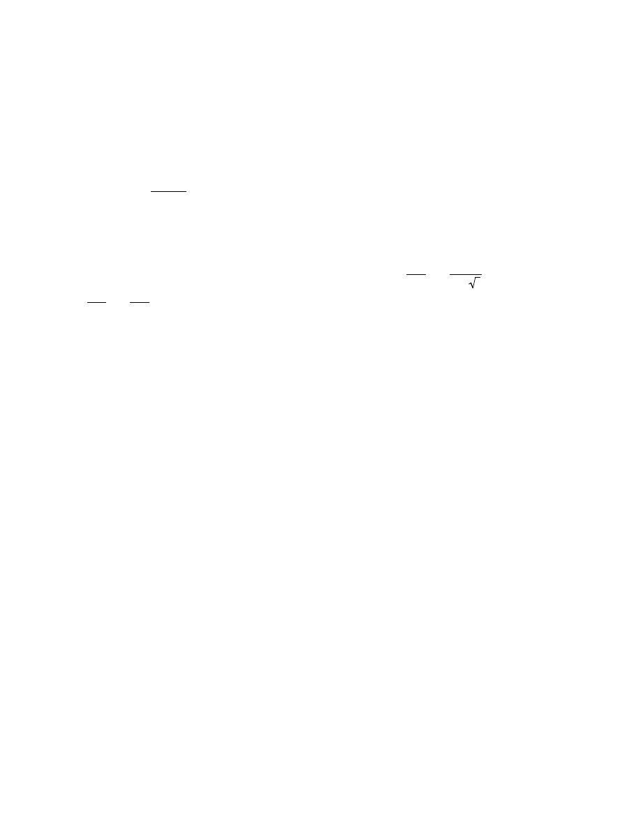
Excerpts from this work may be reproduced by instructors for distribution on a not-for-profit basis for testing or instructional purposes only to
students enrolled in courses for which the textbook has been adopted. Any other reproduction or translation of this work beyond that permitted
by Sections 107 or 108 of the 1976 United States Copyright Act without the permission of the copyright owner is unlawful.
Interfacial Defects
4.27 For an FCC single crystal, would you expect the surface energy for a (100) plane to be greater or
less than that for a (111) plane? Why? (Note: You may want to consult the solution to Problem 3.54 at the end of
Chapter 3.)
Solution
The surface energy for a crystallographic plane will depend on its packing density [i.e., the planar density
(Section 3.11)]—that is, the higher the packing density, the greater the number of nearest-neighbor atoms, and the
more atomic bonds in that plane that are satisfied, and, consequently, the lower the surface energy. From the
solution to Problem 3.54, planar densities for FCC (100) and (111) planes are
1
4R
2
and
1
2R
2
3
, respectively—that
is
0.25
R
2
and
0.29
R
2
(where R is the atomic radius). Thus, since the planar density for (111) is greater, it will have the
lower surface energy.

Excerpts from this work may be reproduced by instructors for distribution on a not-for-profit basis for testing or instructional purposes only to
students enrolled in courses for which the textbook has been adopted. Any other reproduction or translation of this work beyond that permitted
by Sections 107 or 108 of the 1976 United States Copyright Act without the permission of the copyright owner is unlawful.
4.28 For a BCC single crystal, would you expect the surface energy for a (100) plane to be greater or less
than that for a (110) plane? Why? (Note: You may want to consult the solution to Problem 3.55 at the end of
Chapter 3.)
Solution
The surface energy for a crystallographic plane will depend on its packing density [i.e., the planar density
(Section 3.11)]—that is, the higher the packing density, the greater the number of nearest-neighbor atoms, and the
more atomic bonds in that plane that are satisfied, and, consequently, the lower the surface energy. From the
solution to Problem 3.55, the planar densities for BCC (100) and (110) are
3
16R
2
and
3
8R
2
2
, respectively—that
is
0.19
R
2
and
0.27
R
2
. Thus, since the planar density for (110) is greater, it will have the lower surface energy.

Excerpts from this work may be reproduced by instructors for distribution on a not-for-profit basis for testing or instructional purposes only to
students enrolled in courses for which the textbook has been adopted. Any other reproduction or translation of this work beyond that permitted
by Sections 107 or 108 of the 1976 United States Copyright Act without the permission of the copyright owner is unlawful.
4.29 (a) For a given material, would you expect the surface energy to be greater than, the same as, or less
than the grain boundary energy? Why?
(b) The grain boundary energy of a small-angle grain boundary is less than for a high-angle one. Why is
this so?
Solution
(a) The surface energy will be greater than the grain boundary energy. For grain boundaries, some atoms
on one side of a boundary will bond to atoms on the other side; such is not the case for surface atoms. Therefore,
there will be fewer unsatisfied bonds along a grain boundary.
(b) The small-angle grain boundary energy is lower than for a high-angle one because more atoms bond
across the boundary for the small-angle, and, thus, there are fewer unsatisfied bonds.

Excerpts from this work may be reproduced by instructors for distribution on a not-for-profit basis for testing or instructional purposes only to
students enrolled in courses for which the textbook has been adopted. Any other reproduction or translation of this work beyond that permitted
by Sections 107 or 108 of the 1976 United States Copyright Act without the permission of the copyright owner is unlawful.
4.30 (a) Briefly describe a twin and a twin boundary.
(b) Cite the difference between mechanical and annealing twins.
Solution
(a) A twin boundary is an interface such that atoms on one side are located at mirror image positions of
those atoms situated on the other boundary side. The region on one side of this boundary is called a twin.
(b) Mechanical twins are produced as a result of mechanical deformation and generally occur in BCC and
HCP metals. Annealing twins form during annealing heat treatments, most often in FCC metals.
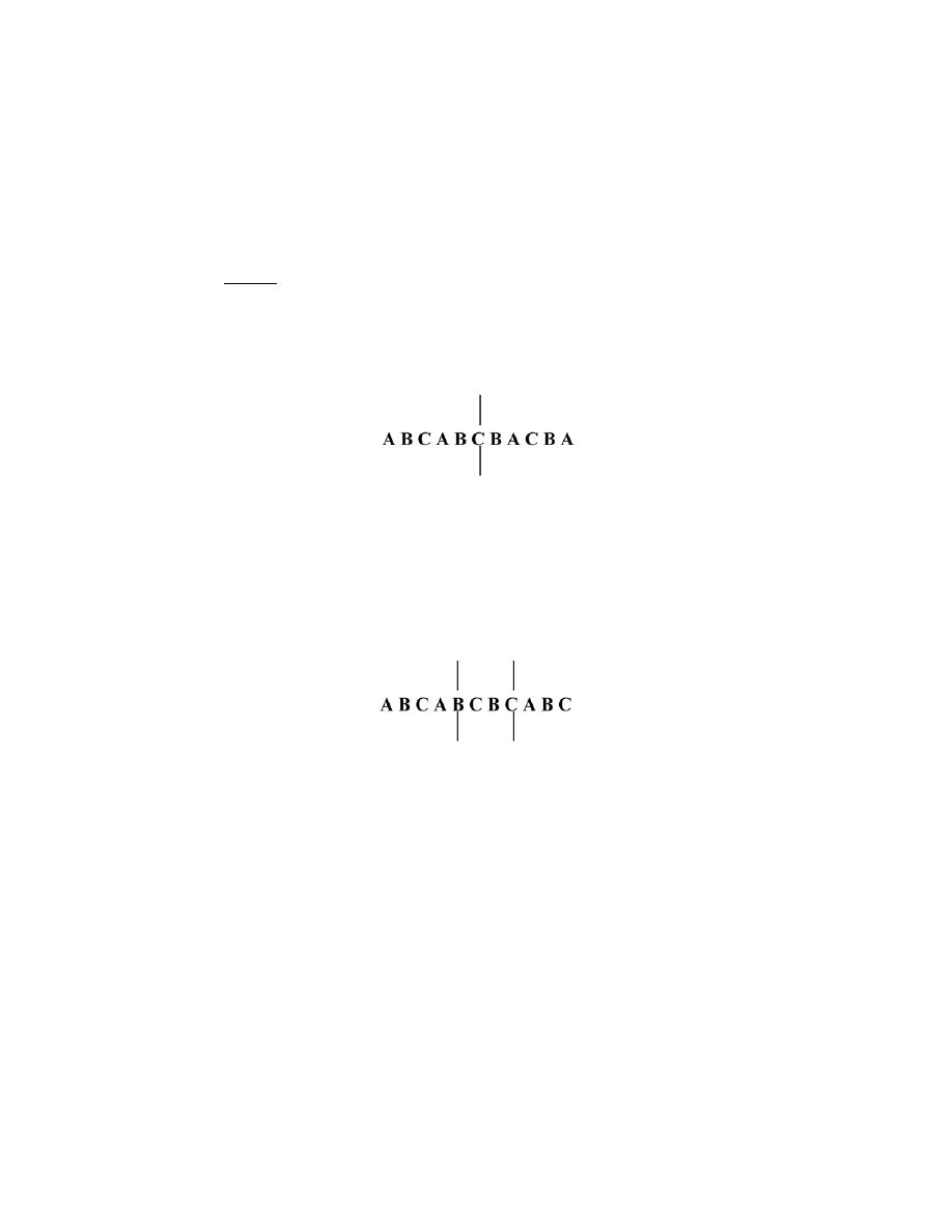
Excerpts from this work may be reproduced by instructors for distribution on a not-for-profit basis for testing or instructional purposes only to
students enrolled in courses for which the textbook has been adopted. Any other reproduction or translation of this work beyond that permitted
by Sections 107 or 108 of the 1976 United States Copyright Act without the permission of the copyright owner is unlawful.
4.31 For each of the following stacking sequences found in FCC metals, cite the type of planar defect that
exists:
(a) . . . A B C A B C B A C B A . . .
(b) . . . A B C A B C B C A B C . . .
Now, copy the stacking sequences and indicate the position(s) of planar defect(s) with a vertical dashed line.
Solution
(a) The interfacial defect that exists for this stacking sequence is a twin boundary, which occurs at the
indicated position.
The stacking sequence on one side of this position is mirrored on the other side.
(b) The interfacial defect that exists within this FCC stacking sequence is a stacking fault, which occurs
between the two lines.
Within this region, the stacking sequence is HCP.

Excerpts from this work may be reproduced by instructors for distribution on a not-for-profit basis for testing or instructional purposes only to
students enrolled in courses for which the textbook has been adopted. Any other reproduction or translation of this work beyond that permitted
by Sections 107 or 108 of the 1976 United States Copyright Act without the permission of the copyright owner is unlawful.
Grain Size Determination
4.32 (a) Using the intercept method, determine the average grain size, in millimeters, of the specimen
whose microstructure is shown in Figure 4.14(b); use at least seven straight-line segments.
(b) Estimate the ASTM grain size number for this material.
Solution
(a) Below is shown the photomicrograph of Figure 4.14(b), on which seven straight line segments, each of
which is 60 mm long has been constructed; these lines are labeled “1” through “7”.
In order to determine the average grain diameter, it is necessary to count the number of grains intersected
by each of these line segments. These data are tabulated below.
Line Number
No. Grains Intersected
1
11
2
10
3
9
4
8.5
5
7
6
10
7
8
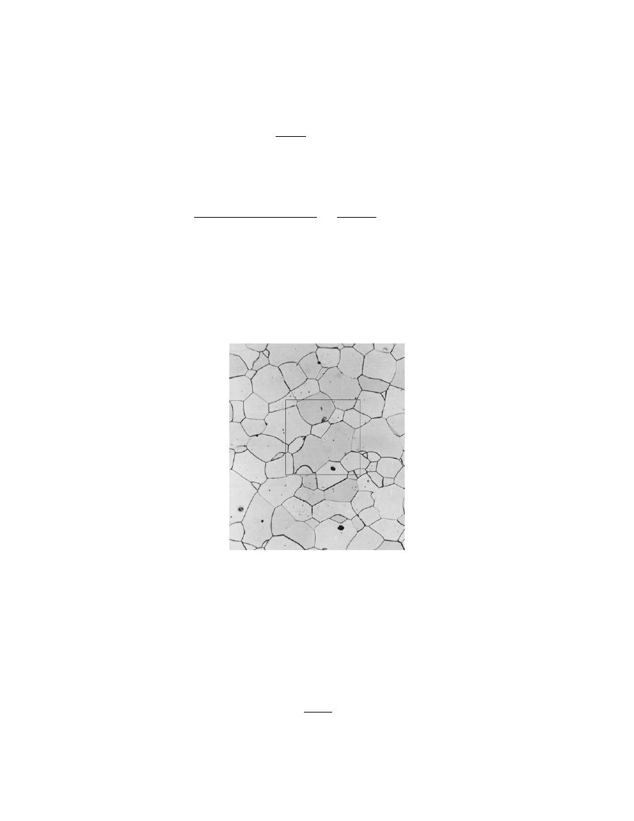
Excerpts from this work may be reproduced by instructors for distribution on a not-for-profit basis for testing or instructional purposes only to
students enrolled in courses for which the textbook has been adopted. Any other reproduction or translation of this work beyond that permitted
by Sections 107 or 108 of the 1976 United States Copyright Act without the permission of the copyright owner is unlawful.
The average number of grain boundary intersections for these lines was 9.1. Therefore, the average line length
intersected is just
60 mm
9.1
= 6.59 mm
Hence, the average grain diameter, d, is
d =
ave. line length intersected
magnification
=
6.59 mm
100
= 6.59
× 10
−2
mm
(b) This portion of the problem calls for us to estimate the ASTM grain size number for this same material.
The average grain size number, n, is related to the number of grains per square inch, N, at a magnification of 100
×
according to Equation 4.16. Inasmuch as the magnification is 100
×, the value of N is measured directly from the
micrograph. The photomicrograph on which has been constructed a square 1 in. on a side is shown below.
The total number of complete grains within this square is approximately 10 (taking into account grain fractions).
Now, in order to solve for n in Equation 4.16, it is first necessary to take logarithms as
log N
= (n − 1) log 2
From which n equals
n
=
log N
log 2
+ 1

Excerpts from this work may be reproduced by instructors for distribution on a not-for-profit basis for testing or instructional purposes only to
students enrolled in courses for which the textbook has been adopted. Any other reproduction or translation of this work beyond that permitted
by Sections 107 or 108 of the 1976 United States Copyright Act without the permission of the copyright owner is unlawful.
=
log 10
log 2
+ 1 = 4.3
Excerpts from this work may be reproduced by instructors for distribution on a not-for-profit basis for testing or instructional purposes only to
students enrolled in courses for which the textbook has been adopted. Any other reproduction or translation of this work beyond that permitted
by Sections 107 or 108 of the 1976 United States Copyright Act without the permission of the copyright owner is unlawful.
4.33 (a) Employing the intercept technique, determine the average grain size for the steel specimen whose
microstructure is shown in Figure 9.25(a); use at least seven straight-line segments.
(b) Estimate the ASTM grain size number for this material.
Solution
(a) Below is shown the photomicrograph of Figure 9.25(a), on which seven straight line segments, each of
which is 60 mm long has been constructed; these lines are labeled “1” through “7”.
In order to determine the average grain diameter, it is necessary to count the number of grains intersected
by each of these line segments. These data are tabulated below.
Line Number
No. Grains Intersected
1
7
2
7
3
7
4
8
5
10
6
7
7
8
The average number of grain boundary intersections for these lines was 8.7. Therefore, the average line length
intersected is just
Excerpts from this work may be reproduced by instructors for distribution on a not-for-profit basis for testing or instructional purposes only to
students enrolled in courses for which the textbook has been adopted. Any other reproduction or translation of this work beyond that permitted
by Sections 107 or 108 of the 1976 United States Copyright Act without the permission of the copyright owner is unlawful.
60 mm
8.7
= 6.9 mm
Hence, the average grain diameter, d, is
d =
ave. line length intersected
magnification
=
6.9 mm
90
= 0.077 mm
(b) This portion of the problem calls for us to estimate the ASTM grain size number for this same material.
The average grain size number, n, is related to the number of grains per square inch, N, at a magnification of 100
×
according to Equation 4.16. However, the magnification of this micrograph is not 100
×, but rather 90×.
Consequently, it is necessary to use Equation 4.17
N
M
M
100
2
= 2
n
−1
where N
M
= the number of grains per square inch at magnification M, and n is the ASTM grain size number.
Taking logarithms of both sides of this equation leads to the following:
log N
M +
2 log
M
100
= (n − 1) log 2
Solving this expression for n gives
n
=
log N
M
+ 2 log
M
100
log 2
+ 1
The photomicrograph on which has been constructed a square 1 in. on a side is shown below.
Excerpts from this work may be reproduced by instructors for distribution on a not-for-profit basis for testing or instructional purposes only to
students enrolled in courses for which the textbook has been adopted. Any other reproduction or translation of this work beyond that permitted
by Sections 107 or 108 of the 1976 United States Copyright Act without the permission of the copyright owner is unlawful.
From Figure 9.25(a), N
M
is measured to be approximately 7, which leads to
n
=
log 7
+ 2 log
90
100
log 2
+ 1
= 3.5

Excerpts from this work may be reproduced by instructors for distribution on a not-for-profit basis for testing or instructional purposes only to
students enrolled in courses for which the textbook has been adopted. Any other reproduction or translation of this work beyond that permitted
by Sections 107 or 108 of the 1976 United States Copyright Act without the permission of the copyright owner is unlawful.
4.34 For an ASTM grain size of 8, approximately how many grains would there be per square inch at
(a) a magnification of 100, and
(b) without any magnification?
Solution
(a) This part of problem asks that we compute the number of grains per square inch for an ASTM grain
size of 8 at a magnification of 100
×. All we need do is solve for the parameter N in Equation 4.16, inasmuch as n =
8. Thus
N
= 2
n
−1
=
2
8
−1
= 128 grains/in.
2
(b) Now it is necessary to compute the value of N for no magnification. In order to solve this problem it is
necessary to use Equation 4.17:
N
M
M
100
2
= 2
n
−1
where NM = the number of grains per square inch at magnification M, and n is the ASTM grain size number.
Without any magnification, M in the above equation is 1, and therefore,
N
1
1
100
2
= 2
8
−1
= 128
And, solving for N
1
, N
1
= 1,280,000 grains/in.
2
.

Excerpts from this work may be reproduced by instructors for distribution on a not-for-profit basis for testing or instructional purposes only to
students enrolled in courses for which the textbook has been adopted. Any other reproduction or translation of this work beyond that permitted
by Sections 107 or 108 of the 1976 United States Copyright Act without the permission of the copyright owner is unlawful.
4.35 Determine the ASTM grain size number if 25 grains per square inch are measured at a magnification
of 600.
Solution
This problem asks that we determine the ASTM grain size number if 8 grains per square inch are measured
at a magnification of 600. In order to solve this problem we make use of Equation 4.17:
N
M
M
100
2
= 2
n
−1
where N
M
= the number of grains per square inch at magnification M, and n is the ASTM grain size number.
Solving the above equation for n, and realizing that N
M
= 8, while M = 600, we have
n
=
log N
M
+ 2 log
M
100
log 2
+ 1
=
log 8
+ 2 log
600
100
log 2
+ 1 = 9.2

Excerpts from this work may be reproduced by instructors for distribution on a not-for-profit basis for testing or instructional purposes only to
students enrolled in courses for which the textbook has been adopted. Any other reproduction or translation of this work beyond that permitted
by Sections 107 or 108 of the 1976 United States Copyright Act without the permission of the copyright owner is unlawful.
4.36 Determine the ASTM grain size number if 20 grains per square inch are measured at a magnification
of 50.
Solution
This problem asks that we determine the ASTM grain size number if 20 grains per square inch are
measured at a magnification of 50. In order to solve this problem we make use of Equation 4.17—viz.
N
M
M
100
2
= 2
n
−1
where N
M
= the number of grains per square inch at magnification M, and n is the ASTM grain size number.
Solving the above equation for n, and realizing that N
M
= 20, while M = 50, we have
n
=
log N
M
+ 2 log
M
100
log 2
+ 1
=
log 20
+ 2 log
50
100
log 2
+ 1 = 3.3

Excerpts from this work may be reproduced by instructors for distribution on a not-for-profit basis for testing or instructional purposes only to
students enrolled in courses for which the textbook has been adopted. Any other reproduction or translation of this work beyond that permitted
by Sections 107 or 108 of the 1976 United States Copyright Act without the permission of the copyright owner is unlawful.
DESIGN PROBLEMS
Specification of Composition
4.D1 Aluminum–lithium alloys have been developed by the aircraft industry to reduce the weight and
improve the performance of its aircraft. A commercial aircraft skin material having a density of 2.55 g/cm
3
is
desired. Compute the concentration of Li (in wt%) that is required.
Solution
Solution of this problem requires the use of Equation 4.10a, which takes the form
ρ
ave
=
100
C
Li
ρ
Li
+
100
− C
Li
ρ
Al
inasmuch as C
Li
+ C
Al
= 100. According to the table inside the front cover, the respective densities of Li and Al
are 0.534 and 2.71 g/cm
3
. Upon solving for C
Li
from the above equation, we get
C
Li
=
100
ρ
Li
(
ρ
Al
− ρ
ave
)
ρ
ave
(
ρ
Al
− ρ
Li
)
And incorporating specified values into the above equation leads to
C
Li
=
(100)
(
0.534 g / cm
3
)(
2.71 g / cm
3
− 2.55 g /cm
3
)
(
2.55 g / cm
3
)(
2.71 g / cm
3
− 0.534 g /cm
3
)
= 1.540 wt%

Excerpts from this work may be reproduced by instructors for distribution on a not-for-profit basis for testing or instructional purposes only to
students enrolled in courses for which the textbook has been adopted. Any other reproduction or translation of this work beyond that permitted
by Sections 107 or 108 of the 1976 United States Copyright Act without the permission of the copyright owner is unlawful.
4.D2 Iron and vanadium both have the BCC crystal structure and V forms a substitutional solid solution
in Fe for concentrations up to approximately 20 wt% V at room temperature. Determine the concentration in
weight percent of V that must be added to iron to yield a unit cell edge length of 0.289 nm.
Solution
To begin, it is necessary to employ Equation 3.5, and solve for the unit cell volume, V
C
, as
V
C
=
nA
ave
ρ
ave
N
A
where A
ave
and
ρ
ave
are the atomic weight and density, respectively, of the Fe-V alloy. Inasmuch as both of these
materials have the BCC crystal structure, which has cubic symmetry, V
C
is just the cube of the unit cell length, a.
That is
V
C
= a
3
= (0.289 nm)
3
= (
2.89
× 10
−8
cm
)
3
= 2.414 × 10
−23
cm
3
It is now necessary to construct expressions for A
ave
and
ρ
ave
in terms of the concentration of vanadium, C
V
, using
Equations 4.11a and 4.10a. For A
ave
we have
A
ave
=
100
C
V
A
V
+
(
100
− C
V
)
A
Fe
=
100
C
V
50.94g / mol
+
(
100
− C
V
)
55.85 g / mol
whereas for
ρ
ave
ρ
ave
=
100
C
V
ρ
V
+
(
100
− C
V
)
ρ
Fe
=
100
C
V
6.10 g / cm
3
+
(
100
− C
V
)
7.87 g / cm
3

Excerpts from this work may be reproduced by instructors for distribution on a not-for-profit basis for testing or instructional purposes only to
students enrolled in courses for which the textbook has been adopted. Any other reproduction or translation of this work beyond that permitted
by Sections 107 or 108 of the 1976 United States Copyright Act without the permission of the copyright owner is unlawful.
Within the BCC unit cell there are 2 equivalent atoms, and thus, the value of n in Equation 3.5 is 2; hence, this
expression may be written in terms of the concentration of V in weight percent as follows:
V
C
= 2.414
× 10
-23
cm3
=
nA
ave
ρ
ave
N
A
=
(2 atoms / unit cell)
100
C
V
50.94 g / mol
+
(
100
− C
V
)
55.85 g / mol
100
C
V
6.10 g / cm
3
+
(
100
− C
V
)
7.87 g / cm
3
(
6.022
× 10
23
atoms / mol
)
And solving this expression for C
V
leads to C
V
= 12.9 wt%.

Excerpts from this work may be reproduced by instructors for distribution on a not-for-profit basis for testing or instructional purposes only to
students enrolled in courses for which the textbook has been adopted. Any other reproduction or translation of this work beyond that permitted
by Sections 107 or 108 of the 1976 United States Copyright Act without the permission of the copyright owner is unlawful.
CHAPTER 5
DIFFUSION
PROBLEM SOLUTIONS
Introduction
5.1 Briefly explain the difference between self-diffusion and interdiffusion.
Solution
Self-diffusion is atomic migration in pure metals--i.e., when all atoms exchanging positions are of the same
type. Interdiffusion is diffusion of atoms of one metal into another metal.

Excerpts from this work may be reproduced by instructors for distribution on a not-for-profit basis for testing or instructional purposes only to
students enrolled in courses for which the textbook has been adopted. Any other reproduction or translation of this work beyond that permitted
by Sections 107 or 108 of the 1976 United States Copyright Act without the permission of the copyright owner is unlawful.
5.2 Self-diffusion involves the motion of atoms that are all of the same type; therefore it is not subject to
observation by compositional changes, as with interdiffusion. Suggest one way in which self-diffusion may be
monitored.
Solution
Self-diffusion may be monitored by using radioactive isotopes of the metal being studied. The motion of
these isotopic atoms may be monitored by measurement of radioactivity level.

Excerpts from this work may be reproduced by instructors for distribution on a not-for-profit basis for testing or instructional purposes only to
students enrolled in courses for which the textbook has been adopted. Any other reproduction or translation of this work beyond that permitted
by Sections 107 or 108 of the 1976 United States Copyright Act without the permission of the copyright owner is unlawful.
Diffusion Mechanisms
5.3 (a) Compare interstitial and vacancy atomic mechanisms for diffusion.
(b) Cite two reasons why interstitial diffusion is normally more rapid than vacancy diffusion.
Solution
(a) With vacancy diffusion, atomic motion is from one lattice site to an adjacent vacancy. Self-diffusion
and the diffusion of substitutional impurities proceed via this mechanism. On the other hand, atomic motion is from
interstitial site to adjacent interstitial site for the interstitial diffusion mechanism.
(b) Interstitial diffusion is normally more rapid than vacancy diffusion because: (1) interstitial atoms,
being smaller, are more mobile; and (2) the probability of an empty adjacent interstitial site is greater than for a
vacancy adjacent to a host (or substitutional impurity) atom.

Excerpts from this work may be reproduced by instructors for distribution on a not-for-profit basis for testing or instructional purposes only to
students enrolled in courses for which the textbook has been adopted. Any other reproduction or translation of this work beyond that permitted
by Sections 107 or 108 of the 1976 United States Copyright Act without the permission of the copyright owner is unlawful.
Steady-State Diffusion
5.4 Briefly explain the concept of steady state as it applies to diffusion.
Solution
Steady-state diffusion is the situation wherein the rate of diffusion into a given system is just equal to the
rate of diffusion out, such that there is no net accumulation or depletion of diffusing species--i.e., the diffusion flux
is independent of time.

Excerpts from this work may be reproduced by instructors for distribution on a not-for-profit basis for testing or instructional purposes only to
students enrolled in courses for which the textbook has been adopted. Any other reproduction or translation of this work beyond that permitted
by Sections 107 or 108 of the 1976 United States Copyright Act without the permission of the copyright owner is unlawful.
5.5 (a) Briefly explain the concept of a driving force.
(b) What is the driving force for steady-state diffusion?
Solution
(a) The driving force is that which compels a reaction to occur.
(b) The driving force for steady-state diffusion is the concentration gradient.

Excerpts from this work may be reproduced by instructors for distribution on a not-for-profit basis for testing or instructional purposes only to
students enrolled in courses for which the textbook has been adopted. Any other reproduction or translation of this work beyond that permitted
by Sections 107 or 108 of the 1976 United States Copyright Act without the permission of the copyright owner is unlawful.
5.6 The purification of hydrogen gas by diffusion through a palladium sheet was discussed in Section 5.3.
Compute the number of kilograms of hydrogen that pass per hour through a 5-mm-thick sheet of palladium having
an area of 0.20 m
2
at 500
°C. Assume a diffusion coefficient of 1.0 × 10
-8
m
2
/s, that the concentrations at the high-
and low-pressure sides of the plate are 2.4 and 0.6 kg of hydrogen per cubic meter of palladium, and that steady-
state conditions have been attained.
Solution
This problem calls for the mass of hydrogen, per hour, that diffuses through a Pd sheet. It first becomes
necessary to employ both Equations 5.1a and 5.3. Combining these expressions and solving for the mass yields
M = JAt =
− DAt
∆C
∆x
=
−
(
1.0
× 10
-8
m
2
/s
)(
0.20 m
2
)
(3600 s/h)
0.6
− 2.4 kg /m
3
5
× 10
−3
m
= 2.6
× 10
-3
kg/h

Excerpts from this work may be reproduced by instructors for distribution on a not-for-profit basis for testing or instructional purposes only to
students enrolled in courses for which the textbook has been adopted. Any other reproduction or translation of this work beyond that permitted
by Sections 107 or 108 of the 1976 United States Copyright Act without the permission of the copyright owner is unlawful.
5.7 A sheet of steel 1.5 mm thick has nitrogen atmospheres on both sides at 1200
°C and is permitted to
achieve a steady-state diffusion condition. The diffusion coefficient for nitrogen in steel at this temperature is 6
×
10
-11
m
2
/s, and the diffusion flux is found to be 1.2
× 10
-7
kg/m
2
-s. Also, it is known that the concentration of
nitrogen in the steel at the high-pressure surface is 4 kg/m
3
. How far into the sheet from this high-pressure side will
the concentration be 2.0 kg/m
3
? Assume a linear concentration profile.
Solution
This problem is solved by using Equation 5.3 in the form
J =
− D
C
A
− C
B
x
A
− x
B
If we take C
A
to be the point at which the concentration of nitrogen is 4 kg/m
3
, then it becomes necessary to solve
for x
B
, as
x
B
= x
A
+ D
C
A
− C
B
J
Assume x
A
is zero at the surface, in which case
x
B
= 0 +
(
6
× 10
-11
m
2
/s
)
4 kg / m
3
− 2 kg /m
3
1.2
× 10
−7
kg / m
2
- s
= 1
× 10
-3
m = 1 mm

Excerpts from this work may be reproduced by instructors for distribution on a not-for-profit basis for testing or instructional purposes only to
students enrolled in courses for which the textbook has been adopted. Any other reproduction or translation of this work beyond that permitted
by Sections 107 or 108 of the 1976 United States Copyright Act without the permission of the copyright owner is unlawful.
5.8 A sheet of BCC iron 1 mm thick was exposed to a carburizing gas atmosphere on one side and a
decarburizing atmosphere on the other side at 725
°C. After having reached steady state, the iron was quickly
cooled to room temperature. The carbon concentrations at the two surfaces of the sheet were determined to be
0.012 and 0.0075 wt%. Compute the diffusion coefficient if the diffusion flux is 1.4
× 10
-8
kg/m
2
-s. Hint: Use
Equation 4.9 to convert the concentrations from weight percent to kilograms of carbon per cubic meter of iron.
Solution
Let us first convert the carbon concentrations from weight percent to kilograms carbon per meter cubed
using Equation 4.9a. For 0.012 wt% C
C
C
"
=
C
C
C
C
ρ
C
+
C
Fe
ρ
Fe
× 10
3
=
0.012
0.012
2.25 g/cm
3
+
99.988
7.87 g/cm
3
× 10
3
0.944 kg C/m
3
Similarly, for 0.0075 wt% C
C
C
"
=
0.0075
0.0075
2.25 g/cm
3
+
99.9925
7.87 g/cm
3
× 10
3
= 0.590 kg C/m
3
Now, using a rearranged form of Equation 5.3
D =
− J
x
A
− x
B
C
A
− C
B
=
−
(
1.40
× 10
-8
kg/m
2
- s
)
− 10
−3
m
0.944 kg/m
3
− 0.590 kg/m
3

Excerpts from this work may be reproduced by instructors for distribution on a not-for-profit basis for testing or instructional purposes only to
students enrolled in courses for which the textbook has been adopted. Any other reproduction or translation of this work beyond that permitted
by Sections 107 or 108 of the 1976 United States Copyright Act without the permission of the copyright owner is unlawful.
= 3.95
× 10
-11
m
2
/s
Excerpts from this work may be reproduced by instructors for distribution on a not-for-profit basis for testing or instructional purposes only to
students enrolled in courses for which the textbook has been adopted. Any other reproduction or translation of this work beyond that permitted
by Sections 107 or 108 of the 1976 United States Copyright Act without the permission of the copyright owner is unlawful.
5.9 When
α-iron is subjected to an atmosphere of hydrogen gas, the concentration of hydrogen in the iron,
C
H
(in weight percent), is a function of hydrogen pressure,
p
H
2
(in MPa), and absolute temperature (T) according
to
C
H
= 1.34 × 10
−2
p
H
2
exp
−
27.2 kJ / mol
RT
(5.14)
Furthermore, the values of D
0
and Q
d
for this diffusion system are 1.4
× 10
-7
m
2
/s and 13,400 J/mol, respectively.
Consider a thin iron membrane 1 mm thick that is at 250
°C. Compute the diffusion flux through this membrane if
the hydrogen pressure on one side of the membrane is 0.15 MPa (1.48 atm), and on the other side 7.5 MPa (74
atm).
Solution
Ultimately we will employ Equation 5.3 to solve this problem. However, it first becomes necessary to
determine the concentration of hydrogen at each face using Equation 5.14. At the low pressure (or B) side
C
H (B)
=
(
1.34
× 10
-2
)
0.15 MPa exp
−
27, 200 J/mol
(8.31 J/mol - K)(250
+ 273 K)
9.93
× 10
-6
wt%
Whereas, for the high pressure (or A) side
C
H (A)
=
(
1.34
× 10
-2
)
7.5 MPa exp
−
27, 200 J/mol
(8.31 J/mol - K)(250
+ 273 K)
7.02
× 10
-5
wt%
We now convert concentrations in weight percent to mass of nitrogen per unit volume of solid. At face B there are
9.93
× 10
-6
g (or 9.93
× 10
-9
kg) of hydrogen in 100 g of Fe, which is virtually pure iron. From the density of iron
(7.87 g/cm3), the volume iron in 100 g (V
B
) is just
V
B
=
100 g
7.87 g /cm
3
= 12.7 cm
3
= 1.27
× 10
-5
m
3
Therefore, the concentration of hydrogen at the B face in kilograms of H per cubic meter of alloy [
C
H (B)
’’
] is just

Excerpts from this work may be reproduced by instructors for distribution on a not-for-profit basis for testing or instructional purposes only to
students enrolled in courses for which the textbook has been adopted. Any other reproduction or translation of this work beyond that permitted
by Sections 107 or 108 of the 1976 United States Copyright Act without the permission of the copyright owner is unlawful.
C
H(B)
''
=
C
H(B)
V
B
=
9.93
× 10
−9
kg
1.27
× 10
−5
m
3
= 7.82
× 10
-4
kg/m
3
At the A face the volume of iron in 100 g (V
A
) will also be 1.27
× 10
-5
m
3
, and
C
H (A)
''
=
C
H(A)
V
A
=
7.02
× 10
−8
kg
1.27
× 10
−5
m
3
= 5.53
× 10
-3
kg/m
3
Thus, the concentration gradient is just the difference between these concentrations of nitrogen divided by the
thickness of the iron membrane; that is
∆C
∆x
=
C
H(B)
''
− C
H(A)
''
x
B
− x
A
=
7.82
× 10
−4
kg / m
3
− 5.53 × 10
−3
kg / m
3
10
−3
m
=
− 4.75 kg/m
4
At this time it becomes necessary to calculate the value of the diffusion coefficient at 250
°C using Equation 5.8.
Thus,
D = D
0
exp
−
Q
d
RT
=
(
1.4
× 10
−7
m
2
/s
)
exp
−
13, 400 J/mol
(8.31 J/mol
− K)(250 + 273 K)
= 6.41
× 10
-9
m
2
/s
And, finally, the diffusion flux is computed using Equation 5.3 by taking the negative product of this diffusion
coefficient and the concentration gradient, as

Excerpts from this work may be reproduced by instructors for distribution on a not-for-profit basis for testing or instructional purposes only to
students enrolled in courses for which the textbook has been adopted. Any other reproduction or translation of this work beyond that permitted
by Sections 107 or 108 of the 1976 United States Copyright Act without the permission of the copyright owner is unlawful.
J =
− D
∆C
∆x
=
−
(
6.41
× 10
-9
m
2
/s
)(
− 4.75 kg/m
4
)
= 3.05
× 10
-8
kg/m
2
- s
Excerpts from this work may be reproduced by instructors for distribution on a not-for-profit basis for testing or instructional purposes only to
students enrolled in courses for which the textbook has been adopted. Any other reproduction or translation of this work beyond that permitted
by Sections 107 or 108 of the 1976 United States Copyright Act without the permission of the copyright owner is unlawful.
Nonsteady-State Diffusion
5.10 Show that
C
x
=
B
Dt
exp
−
x
2
4 Dt
is also a solution to Equation 5.4b. The parameter B is a constant, being independent of both x and t.
Solution
It can be shown that
C
x
=
B
Dt
exp
−
x
2
4 Dt
is a solution to
∂C
∂t
= D
∂
2
C
∂x
2
simply by taking appropriate derivatives of the C
x
expression. When this is carried out,
∂C
∂t
= D
∂
2
C
∂x
2
=
B
2 D
1/ 2
t
3/ 2
x
2
2 Dt
− 1
exp −
x
2
4 Dt
Excerpts from this work may be reproduced by instructors for distribution on a not-for-profit basis for testing or instructional purposes only to
students enrolled in courses for which the textbook has been adopted. Any other reproduction or translation of this work beyond that permitted
by Sections 107 or 108 of the 1976 United States Copyright Act without the permission of the copyright owner is unlawful.
5.11 Determine the carburizing time necessary to achieve a carbon concentration of 0.45 wt% at a
position 2 mm into an iron–carbon alloy that initially contains 0.20 wt% C. The surface concentration is to be
maintained at 1.30 wt% C, and the treatment is to be conducted at 1000
°C. Use the diffusion data for γ-Fe in Table
5.2.
Solution
In order to solve this problem it is first necessary to use Equation 5.5:
C
x
− C
0
C
s
− C
0
= 1
− erf
x
2 Dt
wherein, C
x
= 0.45, C
0
= 0.20, C
s
= 1.30, and x = 2 mm = 2
× 10
-3
m. Thus,
C
x
− C
0
C
s
− C
0
=
0.45
− 0.20
1.30
− 0.20
= 0.2273 = 1
− erf
x
2 Dt
or
erf
x
2 Dt
= 1 − 0.2273 = 0.7727
By linear interpolation using data from Table 5.1
z
erf(z)
0.85
0.7707
z
0.7727
0.90
0.7970
z
− 0.850
0.900
− 0.850
=
0.7727
− 0.7707
0.7970
− 0.7707
From which
z = 0.854 =
x
2 Dt
Now, from Table 5.2, at 1000
°C (1273 K)
Excerpts from this work may be reproduced by instructors for distribution on a not-for-profit basis for testing or instructional purposes only to
students enrolled in courses for which the textbook has been adopted. Any other reproduction or translation of this work beyond that permitted
by Sections 107 or 108 of the 1976 United States Copyright Act without the permission of the copyright owner is unlawful.
D =
(
2.3
× 10
-5
m
2
/s
)
exp
−
148, 000 J/mol
(8.31 J/mol - K)(1273 K)
= 1.93
× 10
-11
m
2
/s
Thus,
0.854 =
2
× 10
−3
m
(2)
(
1.93
× 10
−11
m
2
/s
)
(t)
Solving for t yields
t = 7.1
× 10
4
s = 19.7 h
Excerpts from this work may be reproduced by instructors for distribution on a not-for-profit basis for testing or instructional purposes only to
students enrolled in courses for which the textbook has been adopted. Any other reproduction or translation of this work beyond that permitted
by Sections 107 or 108 of the 1976 United States Copyright Act without the permission of the copyright owner is unlawful.
5.12 An FCC iron-carbon alloy initially containing 0.35 wt% C is exposed to an oxygen-rich and virtually
carbon-free atmosphere at 1400 K (1127
°C). Under these circumstances the carbon diffuses from the alloy and
reacts at the surface with the oxygen in the atmosphere; that is, the carbon concentration at the surface position is
maintained essentially at 0 wt% C. (This process of carbon depletion is termed decarburization.) At what position
will the carbon concentration be 0.15 wt% after a 10-h treatment? The value of D at 1400 K is 6.9
× 10
-11
m
2
/s.
Solution
This problem asks that we determine the position at which the carbon concentration is 0.15 wt% after a 10-
h heat treatment at 1325 K when C
0
= 0.35 wt% C. From Equation 5.5
C
x
− C
0
C
s
− C
0
=
0.15
− 0.35
0
− 0.35
= 0.5714 = 1
− erf
x
2 Dt
Thus,
erf
x
2 Dt
= 0.4286
Using data in Table 5.1 and linear interpolation
z
erf (z)
0.40
0.4284
z
0.4286
0.45
0.4755
z
− 0.40
0.45
− 0.40
=
0.4286
− 0.4284
0.4755
− 0.4284
And,
z = 0.4002
Which means that
x
2 Dt
= 0.4002
And, finally

Excerpts from this work may be reproduced by instructors for distribution on a not-for-profit basis for testing or instructional purposes only to
students enrolled in courses for which the textbook has been adopted. Any other reproduction or translation of this work beyond that permitted
by Sections 107 or 108 of the 1976 United States Copyright Act without the permission of the copyright owner is unlawful.
x = 2(0.4002) Dt = (0.8004)
(
6.9
× 10
−11
m
2
/s
)(
3.6
× 10
4
s
)
= 1.26
× 10
-3
m = 1.26 mm
Note: this problem may also be solved using the “Diffusion” module in the VMSE software. Open the “Diffusion”
module, click on the “Diffusion Design” submodule, and then do the following:
1. Enter the given data in left-hand window that appears. In the window below the label “D Value” enter
the value of the diffusion coefficient—viz. “6.9e-11”.
2. In the window just below the label “Initial, C
0
” enter the initial concentration—viz. “0.35”.
3. In the window the lies below “Surface, C
s
” enter the surface concentration—viz. “0”.
4. Then in the “Diffusion Time t” window enter the time in seconds; in 10 h there are (60 s/min)(60
min/h)(10 h) = 36,000 s—so enter the value “3.6e4”.
5. Next, at the bottom of this window click on the button labeled “Add curve”.
6. On the right portion of the screen will appear a concentration profile for this particular diffusion
situation. A diamond-shaped cursor will appear at the upper left-hand corner of the resulting curve. Click and drag
this cursor down the curve to the point at which the number below “Concentration:” reads “0.15 wt%”. Then read
the value under the “Distance:”. For this problem, this value (the solution to the problem) is ranges between 1.24
and 1.30 mm.
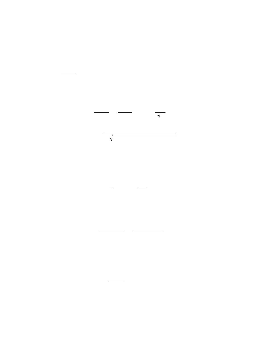
Excerpts from this work may be reproduced by instructors for distribution on a not-for-profit basis for testing or instructional purposes only to
students enrolled in courses for which the textbook has been adopted. Any other reproduction or translation of this work beyond that permitted
by Sections 107 or 108 of the 1976 United States Copyright Act without the permission of the copyright owner is unlawful.
5.13 Nitrogen from a gaseous phase is to be diffused into pure iron at 700
°C. If the surface concentration
is maintained at 0.1 wt% N, what will be the concentration 1 mm from the surface after 10 h? The diffusion
coefficient for nitrogen in iron at 700
°C is 2.5 × 10
-11
m
2
/s.
Solution
This problem asks us to compute the nitrogen concentration (C
x
) at the 1 mm position after a 10 h diffusion
time, when diffusion is nonsteady-state. From Equation 5.5
C
x
− C
0
C
s
− C
0
=
C
x
− 0
0.1
− 0
= 1
− erf
x
2 Dt
= 1
− erf
10
−3
m
(2)
(
2.5
× 10
−11
m
2
/s
)
(10 h)(3600 s / h)
= 1 – erf (0.527)
Using data in Table 5.1 and linear interpolation
z
erf (z)
0.500
0.5205
0.527
y
0.550
0.5633
0.527
− 0.500
0.550
− 0.500
=
y
− 0.5205
0.5633
− 0.5205
from which
y = erf (0.527) = 0.5436
Thus,
C
x
− 0
0.1
− 0
= 1.0
− 0.5436

Excerpts from this work may be reproduced by instructors for distribution on a not-for-profit basis for testing or instructional purposes only to
students enrolled in courses for which the textbook has been adopted. Any other reproduction or translation of this work beyond that permitted
by Sections 107 or 108 of the 1976 United States Copyright Act without the permission of the copyright owner is unlawful.
This expression gives
C
x
= 0.046 wt% N
Note: this problem may also be solved using the “Diffusion” module in the VMSE software. Open the “Diffusion”
module, click on the “Diffusion Design” submodule, and then do the following:
1. Enter the given data in left-hand window that appears. In the window below the label “D Value” enter
the value of the diffusion coefficient—viz. “2.5e-11”.
2. In the window just below the label “Initial, C
0
” enter the initial concentration—viz. “0”.
3. In the window the lies below “Surface, C
s
” enter the surface concentration—viz. “0.1”.
4. Then in the “Diffusion Time t” window enter the time in seconds; in 10 h there are (60 s/min)(60
min/h)(10 h) = 36,000 s—so enter the value “3.6e4”.
5. Next, at the bottom of this window click on the button labeled “Add curve”.
6. On the right portion of the screen will appear a concentration profile for this particular diffusion
situation. A diamond-shaped cursor will appear at the upper left-hand corner of the resulting curve. Click and drag
this cursor down the curve to the point at which the number below “Distance:” reads “1.00 mm”. Then read the
value under the “Concentration:”. For this problem, this value (the solution to the problem) is 0.05 wt%.
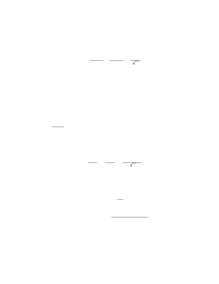
Excerpts from this work may be reproduced by instructors for distribution on a not-for-profit basis for testing or instructional purposes only to
students enrolled in courses for which the textbook has been adopted. Any other reproduction or translation of this work beyond that permitted
by Sections 107 or 108 of the 1976 United States Copyright Act without the permission of the copyright owner is unlawful.
5.14 Consider a diffusion couple composed of two semi-infinite solids of the same metal, and that each
side of the diffusion couple has a different concentration of the same elemental impurity; furthermore, assume each
impurity level is constant throughout its side of the diffusion couple. For this situation, the solution to Fick’s second
law (assuming that the diffusion coefficient for the impurity is independent of concentration), is as follows:
C
x
=
C
1
+ C
2
2
−
C
1
− C
2
2
erf
x
2 Dt
(5.15)
In this expression, when the x = 0 position is taken as the initial diffusion couple interface, then C
1
is the impurity
concentration for x < 0; likewise, C
2
is the impurity content for x > 0.
A diffusion couple composed of two silver-gold alloys is formed; these alloys have compositions of 98 wt%
Ag–2 wt% Au and 95 wt% Ag–5 wt% Au. Determine the time this diffusion couple must be heated at 750ºC (1023 K)
in order for the composition to be 2.5 wt% Au at the 50 mm position into the 2 wt% Au side of the diffusion couple.
Preexponential and activation energy values for Au diffusion in Ag are 8.5
× 10
–5
m
2
/s and 202,100 J/mol,
respectively.
Solution
For this platinum-gold diffusion couple for which C
1
= 5 wt% Au and C
2
= 2 wt% Au, we are asked to
determine the diffusion time at 750
°C that will give a composition of 2.5 wt% Au at the 50 µm position. Thus, for
this problem, Equation 5.15 takes the form
2.5 =
5
+ 2
2
−
5
− 2
2
erf
50
× 10
−6
m
2 Dt
It now becomes necessary to compute the diffusion coefficient at 750
°C (1023 K) given that D
0
= 8.5
× 10
-5
m
2
/s
and Q
d
= 202,100 J/mol. From Equation 5.8 we have
D = D
0
exp
−
Q
d
RT
=
(
8.5
× 10
-5
m
2
/s
)
exp
−
202,100 J/mol
(8.31 J/mol
− K)(1023 K)
= 4.03
× 10
-15
m
2
/s
Substitution of this value into the above equation leads to
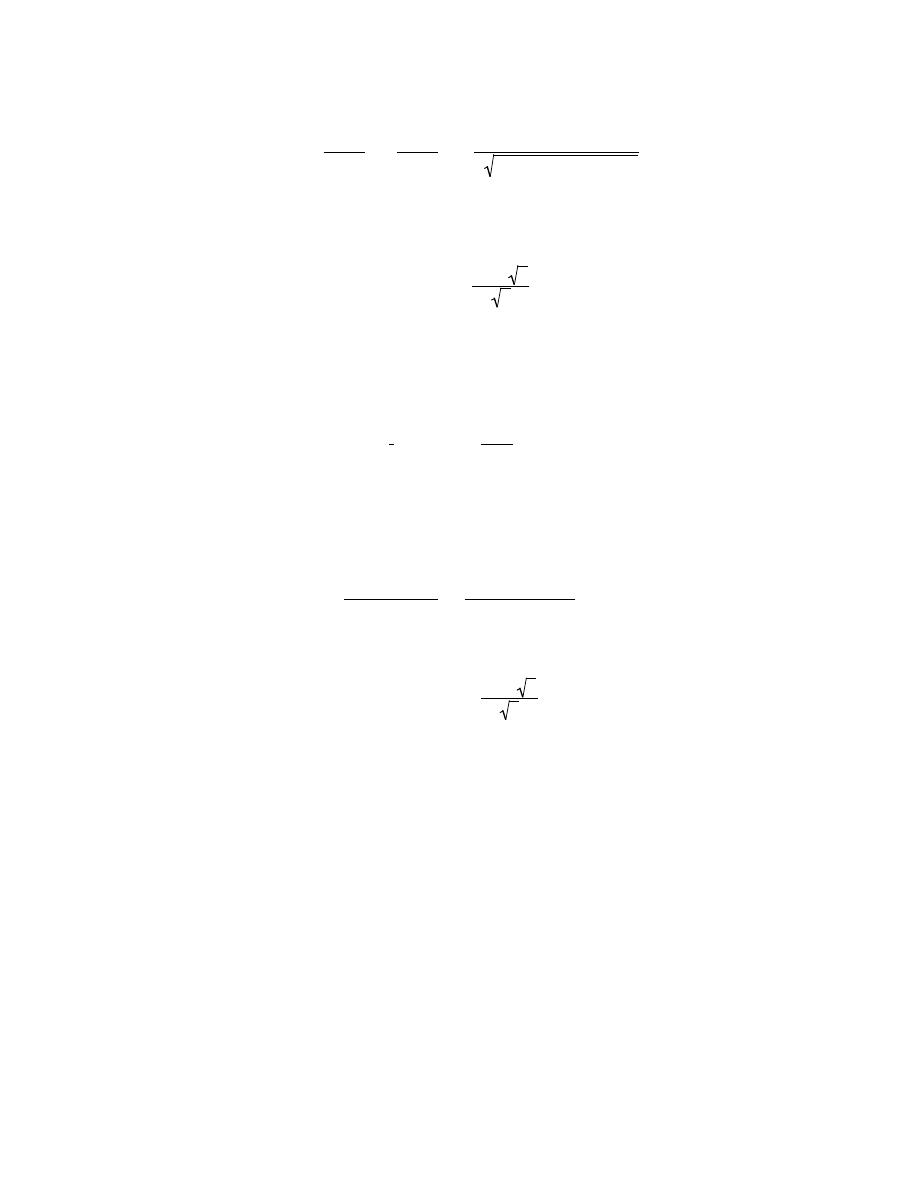
Excerpts from this work may be reproduced by instructors for distribution on a not-for-profit basis for testing or instructional purposes only to
students enrolled in courses for which the textbook has been adopted. Any other reproduction or translation of this work beyond that permitted
by Sections 107 or 108 of the 1976 United States Copyright Act without the permission of the copyright owner is unlawful.
2.5 =
5
+ 2
2
−
5
− 2
2
erf
50
× 10
−6
m
2
(
4.03
× 10
−15
m
2
/s
)
(t)
This expression reduces to the following form:
0.6667 = erf
393.8 s
t
Using data in Table 5.1, it is necessary to determine the value of z for which the error function is 0.6667 We use
linear interpolation as follows:
z
erf (z)
0.650
0.6420
y
0.6667
0.700
0.6778
y
− 0.650
0.700
− 0.650
=
0.6667
− 0.6420
0.6778
− 0.6420
from which
y = 0.6844 =
393.8 s
t
And, solving for t gives
t = 3.31
× 10
5
s = 92 h
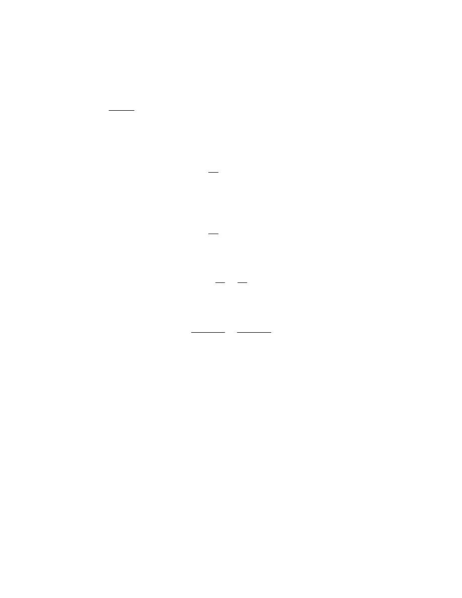
Excerpts from this work may be reproduced by instructors for distribution on a not-for-profit basis for testing or instructional purposes only to
students enrolled in courses for which the textbook has been adopted. Any other reproduction or translation of this work beyond that permitted
by Sections 107 or 108 of the 1976 United States Copyright Act without the permission of the copyright owner is unlawful.
5.15 For a steel alloy it has been determined that a carburizing heat treatment of 10-h duration will raise
the carbon concentration to 0.45 wt% at a point 2.5 mm from the surface. Estimate the time necessary to achieve
the same concentration at a 5.0-mm position for an identical steel and at the same carburizing temperature.
Solution
This problem calls for an estimate of the time necessary to achieve a carbon concentration of 0.45 wt% at a
point 5.0 mm from the surface. From Equation 5.6b,
x
2
Dt
= constant
But since the temperature is constant, so also is D constant, and
x
2
t
= constant
or
x
1
2
t
1
=
x
2
2
t
2
Thus,
(2.5 mm)
2
10 h
=
(5.0 mm)
2
t
2
from which
t2 = 40 h

Excerpts from this work may be reproduced by instructors for distribution on a not-for-profit basis for testing or instructional purposes only to
students enrolled in courses for which the textbook has been adopted. Any other reproduction or translation of this work beyond that permitted
by Sections 107 or 108 of the 1976 United States Copyright Act without the permission of the copyright owner is unlawful.
Factors That Influence Diffusion
5.16 Cite the values of the diffusion coefficients for the interdiffusion of carbon in both
α-iron (BCC) and
γ-iron (FCC) at 900°C. Which is larger? Explain why this is the case.
Solution
We are asked to compute the diffusion coefficients of C in both
α and γ iron at 900°C. Using the data in
Table 5.2,
D
α
=
(
6.2
× 10
-7
m
2
/s
)
exp
−
80, 000 J/mol
(8.31 J/mol - K)(1173 K)
= 1.69
× 10
-10
m
2
/s
D
γ
=
(
2.3
× 10
-5
m
2
/s
)
exp
−
148, 000 J/mol
(8.31 J/mol - K)(1173 K)
= 5.86
× 10
-12
m
2
/s
The D for diffusion of C in BCC
α iron is larger, the reason being that the atomic packing factor is smaller
than for FCC
γ iron (0.68 versus 0.74—Section 3.4); this means that there is slightly more interstitial void space in
the BCC Fe, and, therefore, the motion of the interstitial carbon atoms occurs more easily.

Excerpts from this work may be reproduced by instructors for distribution on a not-for-profit basis for testing or instructional purposes only to
students enrolled in courses for which the textbook has been adopted. Any other reproduction or translation of this work beyond that permitted
by Sections 107 or 108 of the 1976 United States Copyright Act without the permission of the copyright owner is unlawful.
5.17 Using the data in Table 5.2, compute the value of D for the diffusion of zinc in copper at 650ºC.
Solution
Incorporating the appropriate data from Table 5.2 into Equation 5.8 leads to
D =
(
2.4
× 10
-5
m
2
/s
)
exp
−
189, 000 J/mol
(8.31 J/mol - K)(650
+ 273 K)
= 4.8
× 10
-16
m
2
/s
Note: this problem may also be solved using the “Diffusion” module in the VMSE software. Open the “Diffusion”
module, click on the “D vs 1/T Plot” submodule, and then do the following:
1. In the left-hand window that appears, click on the “Zn-Cu” pair under the “Diffusing Species”-“Host
Metal” headings.
2. Next, at the bottom of this window, click the “Add Curve” button.
3. A log D versus 1/T plot then appears, with a line for the temperature dependence of the diffusion
coefficient for Zn in Cu. Now under “Temp Range” in the boxes appearing below “T Max” change the temperature
to either “650” C or “923” K. At the top of this curve is a diamond-shaped cursor. Click-and-drag this cursor down
the line to the point at which the entry under the “Temperature (T):” label reads 923 K (inasmuch as this is the
Kelvin equivalent of 650ºC). Finally, the diffusion coefficient value at this temperature is given under the label
“Diff Coeff (D):”. For this problem, the value is 4.7
× 10
-16
m
2
/s.

Excerpts from this work may be reproduced by instructors for distribution on a not-for-profit basis for testing or instructional purposes only to
students enrolled in courses for which the textbook has been adopted. Any other reproduction or translation of this work beyond that permitted
by Sections 107 or 108 of the 1976 United States Copyright Act without the permission of the copyright owner is unlawful.
5.18 At what temperature will the diffusion coefficient for the diffusion of copper in nickel have a value of
6.5
× 10
-17
m
2
/s. Use the diffusion data in Table 5.2.
Solution
Solving for T from Equation 5.9a
T =
−
Q
d
R
(
ln D
− ln D
0
)
and using the data from Table 5.2 for the diffusion of Cu in Ni (i.e., D
0
= 2.7
× 10
-5
m
2
/s and Q
d
= 256,000 J/mol) ,
we get
T =
−
256, 000 J/mol
(8.31 J/mol - K) ln
(
6.5
× 10
-17
m
2
/s
)
− ln
(
2.7
× 10
-5
m
2
/s
)
[
]
= 1152 K = 879
°C
Note: this problem may also be solved using the “Diffusion” module in the VMSE software. Open the “Diffusion”
module, click on the “D vs 1/T Plot” submodule, and then do the following:
1. In the left-hand window that appears, there is a preset set of data for several diffusion systems. Click on
the box for which Cu is the diffusing species and Ni is the host metal. Next, at the bottom of this window, click the
“Add Curve” button.
2. A log D versus 1/T plot then appears, with a line for the temperature dependence of the diffusion
coefficient for Cu in Ni. At the top of this curve is a diamond-shaped cursor. Click-and-drag this cursor down the
line to the point at which the entry under the “Diff Coeff (D):” label reads 6.5
× 10
-17
m
2
/s. The temperature at
which the diffusion coefficient has this value is given under the label “Temperature (T):”. For this problem, the
value is 1153 K.

Excerpts from this work may be reproduced by instructors for distribution on a not-for-profit basis for testing or instructional purposes only to
students enrolled in courses for which the textbook has been adopted. Any other reproduction or translation of this work beyond that permitted
by Sections 107 or 108 of the 1976 United States Copyright Act without the permission of the copyright owner is unlawful.
5.19 The preexponential and activation energy for the diffusion of iron in cobalt are 1.1
× 10
-5
m
2
/s and
253,300 J/mol, respectively. At what temperature will the diffusion coefficient have a value of 2.1
× 10
-14
m
2
/s?
Solution
For this problem we are given D
0
(1.1
× 10
-5
) and Q
d
(253,300 J/mol) for the diffusion of Fe in Co, and
asked to compute the temperature at which D = 2.1
× 10
-14
m
2
/s. Solving for T from Equation 5.9a yields
T =
Q
d
R
(
ln D
0
− ln D
)
=
253, 300 J/mol
(8.31 J/mol - K) ln
(
1.1
× 10
-5
m
2
/s
)
- ln
(
2.1
× 10
-14
m
2
/s
)
[
]
= 1518 K = 1245
°C
Note: this problem may also be solved using the “Diffusion” module in the VMSE software. Open the “Diffusion”
module, click on the “D vs 1/T Plot” submodule, and then do the following:
1. In the left-hand window that appears, click on the “Custom1” box.
2. In the column on the right-hand side of this window enter the data for this problem. In the window
under “D
0
” enter preexponential value—viz. “1.1e-5”. Next just below the “Q
d
” window enter the activation
energy value—viz. “253.3”. It is next necessary to specify a temperature range over which the data is to be plotted.
The temperature at which D has the stipulated value is probably between 1000ºC and 1500ºC, so enter “1000” in the
“T Min” box that is beside “C”; and similarly for the maximum temperature—enter “1500” in the box below “T
Max”.
3. Next, at the bottom of this window, click the “Add Curve” button.
4. A log D versus 1/T plot then appears, with a line for the temperature dependence of the diffusion
coefficient for Fe in Co. At the top of this curve is a diamond-shaped cursor. Click-and-drag this cursor down the
line to the point at which the entry under the “Diff Coeff (D):” label reads 2.1
× 10
-14
m
2
/s. The temperature at
which the diffusion coefficient has this value is given under the label “Temperature (T):”. For this problem, the
value is 1519 K.

Excerpts from this work may be reproduced by instructors for distribution on a not-for-profit basis for testing or instructional purposes only to
students enrolled in courses for which the textbook has been adopted. Any other reproduction or translation of this work beyond that permitted
by Sections 107 or 108 of the 1976 United States Copyright Act without the permission of the copyright owner is unlawful.
5.20 The activation energy for the diffusion of carbon in chromium is 111,000 J/mol. Calculate the
diffusion coefficient at 1100 K (827
°C), given that D at 1400 K (1127°C) is 6.25 × 10
-11
m
2
/s.
Solution
To solve this problem it first becomes necessary to solve for D
0
from Equation 5.8 as
D
0
= D exp
Q
d
RT
=
(
6.25
× 10
-11
m
2
/s
)
exp
111, 000 J / mol
(8.31 J/mol - K)(1400 K)
= 8.7
× 10
-7
m
2
/s
Now, solving for D at 1100 K (again using Equation 5.8) gives
D =
(
8.7
× 10
-7
m
2
/s
)
exp
−
111, 000 J/mol
(8.31 J/mol - K)(1100 K)
= 4.6
× 10
-12
m
2
/s

Excerpts from this work may be reproduced by instructors for distribution on a not-for-profit basis for testing or instructional purposes only to
students enrolled in courses for which the textbook has been adopted. Any other reproduction or translation of this work beyond that permitted
by Sections 107 or 108 of the 1976 United States Copyright Act without the permission of the copyright owner is unlawful.
5.21 The diffusion coefficients for iron in nickel are given at two temperatures:
T (K)
D (m
2
/s)
1273
9.4 × 10
–16
1473
2.4 × 10
–14
(a) Determine the values of D
0
and the activation energy Q
d
.
(b) What is the magnitude of D at 1100ºC (1373 K)?
Solution
(a) Using Equation 5.9a, we set up two simultaneous equations with Q
d
and D
0
as unknowns as follows:
ln D
1
= lnD
0
−
Q
d
R
1
T
1
ln D
2
= lnD
0
−
Q
d
R
1
T
2
Now, solving for Q
d
in terms of temperatures T
1
and T
2
(1273
K and 1473
K) and D
1
and D
2
(9.4
× 10
-16
and 2.4
×
10
-14
m
2
/s), we get
Q
d
=
− R
ln D
1
− ln D
2
1
T
1
−
1
T
2
=
− (8.31 J/mol - K)
ln
(
9.4
× 10
-16
)
− ln
(
2.4
× 10
-14
)
[
]
1
1273 K
−
1
1473 K
= 252,400 J/mol
Now, solving for D
0
from Equation 5.8 (and using the 1273 K value of D)
D
0
= D
1
exp
Q
d
RT
1

Excerpts from this work may be reproduced by instructors for distribution on a not-for-profit basis for testing or instructional purposes only to
students enrolled in courses for which the textbook has been adopted. Any other reproduction or translation of this work beyond that permitted
by Sections 107 or 108 of the 1976 United States Copyright Act without the permission of the copyright owner is unlawful.
=
(
9.4
× 10
-16
m
2
/s
)
exp
252, 400 J/mol
(8.31 J/mol - K)(1273 K)
= 2.2
× 10
-5
m
2
/s
(b) Using these values of D
0
and Q
d
, D at 1373
K is just
D =
(
2.2
× 10
-5
m
2
/s
)
exp
−
252, 400 J/mol
(8.31 J/mol - K)(1373 K)
= 5.4
× 10
-15
m
2
/s
Note: this problem may also be solved using the “Diffusion” module in the VMSE software. Open the “Diffusion”
module, click on the “D
0
and Q
d
from Experimental Data” submodule, and then do the following:
1. In the left-hand window that appears, enter the two temperatures from the table in the book (viz. “1273”
and “1473”, in the first two boxes under the column labeled “T (K)”. Next, enter the corresponding diffusion
coefficient values (viz. “9.4e-16” and “2.4e-14”).
3. Next, at the bottom of this window, click the “Plot data” button.
4. A log D versus 1/T plot then appears, with a line for the temperature dependence for this diffusion
system. At the top of this window are give values for D
0
and Q
d
; for this specific problem these values are 2.17
×
10
-5
m
2
/s and 252 kJ/mol, respectively
5. To solve the (b) part of the problem we utilize the diamond-shaped cursor that is located at the top of
the line on this plot. Click-and-drag this cursor down the line to the point at which the entry under the “Temperature
(T):” label reads “1373”. The value of the diffusion coefficient at this temperature is given under the label “Diff
Coeff (D):”. For our problem, this value is 5.4
× 10
-15
m
2
/s.

Excerpts from this work may be reproduced by instructors for distribution on a not-for-profit basis for testing or instructional purposes only to
students enrolled in courses for which the textbook has been adopted. Any other reproduction or translation of this work beyond that permitted
by Sections 107 or 108 of the 1976 United States Copyright Act without the permission of the copyright owner is unlawful.
5.22 The diffusion coefficients for silver in copper are given at two temperatures:
T (°C)
D (m
2
/s)
650
5.5 × 10
–16
900
1.3 × 10
–13
(a) Determine the values of D
0
and Q
d
.
(b) What is the magnitude of D at 875°C?
Solution
(a) Using Equation 5.9a, we set up two simultaneous equations with Q
d
and D
0
as unknowns as follows:
ln D
1
= lnD
0
−
Q
d
R
1
T
1
ln D
2
= lnD
0
−
Q
d
R
1
T
2
Solving for Q
d
in terms of temperatures T
1
and T
2
(923
K [650
°C] and 1173 K [900°C]) and D
1
and D
2
(5.5
× 10
-
16
and 1.3
× 10
-13
m
2
/s), we get
Q
d
=
− R
ln D
1
− ln D
2
1
T
1
−
1
T
2
=
−
(8.31 J/mol - K) ln
(
5.5
× 10
-16
)
− ln
(
1.3
× 10
-13
)
[
]
1
923 K
−
1
1173 K
= 196,700 J/mol
Now, solving for D
0
from Equation 5.8 (and using the 650
°C value of D)
D
0
= D
1
exp
Q
d
RT
1

Excerpts from this work may be reproduced by instructors for distribution on a not-for-profit basis for testing or instructional purposes only to
students enrolled in courses for which the textbook has been adopted. Any other reproduction or translation of this work beyond that permitted
by Sections 107 or 108 of the 1976 United States Copyright Act without the permission of the copyright owner is unlawful.
=
(
5.5
× 10
-16
m
2
/s
)
exp
196, 700 J/mol
(8.31 J/mol - K)(923 K)
= 7.5
× 10
-5
m
2
/s
(b) Using these values of D
0
and Q
d
, D at 1148
K (875
°C) is just
D =
(
7.5
× 10
-5
m
2
/s
)
exp
−
196, 700 J/mol
(8.31 J/mol - K)(1148 K)
= 8.3
× 10
-14
m
2
/s
Note: this problem may also be solved using the “Diffusion” module in the VMSE software. Open the “Diffusion”
module, click on the “D
0
and Q
d
from Experimental Data” submodule, and then do the following:
1. In the left-hand window that appears, enter the two temperatures from the table in the book (converted
from degrees Celsius to Kelvins) (viz. “923” (650ºC) and “1173” (900ºC), in the first two boxes under the column
labeled “T (K)”. Next, enter the corresponding diffusion coefficient values (viz. “5.5e-16” and “1.3e-13”).
3. Next, at the bottom of this window, click the “Plot data” button.
4. A log D versus 1/T plot then appears, with a line for the temperature dependence for this diffusion
system. At the top of this window are give values for D
0
and Q
d
; for this specific problem these values are 7.55
×
10
-5
m
2
/s and 196 kJ/mol, respectively
5. To solve the (b) part of the problem we utilize the diamond-shaped cursor that is located at the top of
the line on this plot. Click-and-drag this cursor down the line to the point at which the entry under the “Temperature
(T):” label reads “1148” (i.e., 875ºC). The value of the diffusion coefficient at this temperature is given under the
label “Diff Coeff (D):”. For our problem, this value is 8.9
× 10
-14
m
2
/s.
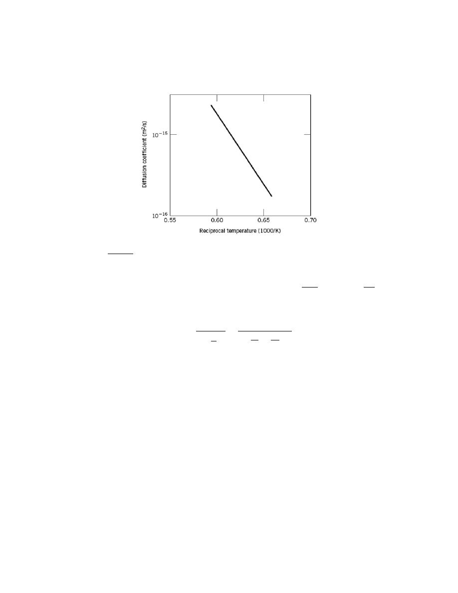
Excerpts from this work may be reproduced by instructors for distribution on a not-for-profit basis for testing or instructional purposes only to
students enrolled in courses for which the textbook has been adopted. Any other reproduction or translation of this work beyond that permitted
by Sections 107 or 108 of the 1976 United States Copyright Act without the permission of the copyright owner is unlawful.
5.23 Below is shown a plot of the logarithm (to the base 10) of the diffusion coefficient versus reciprocal
of the absolute temperature, for the diffusion of iron in chromium. Determine values for the activation energy and
preexponential.
Solution
This problem asks us to determine the values of Q
d
and D
0
for the diffusion of Fe in Cr from the plot of
log D versus 1/T. According to Equation 5.9b the slope of this plot is equal to
−
Q
d
2.3 R
(rather than
−
Q
d
R
since we
are using log D rather than ln D) and the intercept at 1/T = 0 gives the value of log D
0
. The slope is equal to
slope =
∆ (log D)
∆
1
T
=
log D
1
− log D
2
1
T
1
−
1
T
2
Taking 1/T
1
and 1/T
2
as 0.65
× 10
-3
and 0.60
× 10
-3
K
-1
, respectively, then the corresponding values of D
1
and D
2
are 2.81
× 10
-16
and 1.82
× 10
-15
, as noted in the figure below.
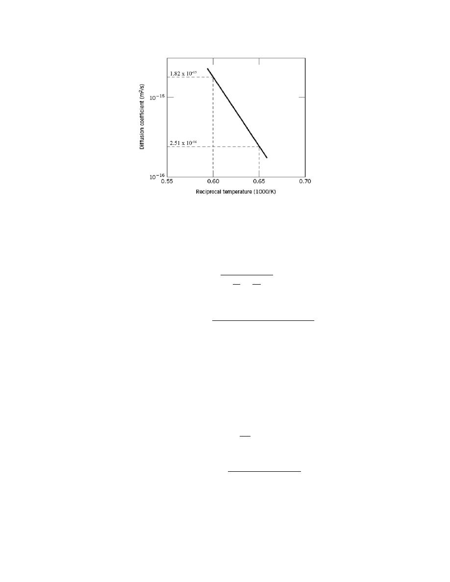
Excerpts from this work may be reproduced by instructors for distribution on a not-for-profit basis for testing or instructional purposes only to
students enrolled in courses for which the textbook has been adopted. Any other reproduction or translation of this work beyond that permitted
by Sections 107 or 108 of the 1976 United States Copyright Act without the permission of the copyright owner is unlawful.
The values of log D
1
and log D
2
are –15.60 and –14.74, and therefore,
Q
d
=
− 2.3 R (slope)
Q
d
=
− 2.3 R
log D
1
− log D
2
1
T
1
−
1
T
2
=
− (2.3)(8.31 J/mol - K)
−15.60 − (−14.74)
(
0.65
× 10
−3
− 0.60 × 10
−3
)
K
−1
= 329,000 J/mol
Rather than trying to make a graphical extrapolation to determine D
0
, a more accurate value is obtained
analytically using Equation 5.9b taking a specific value of both D and T (from 1/T) from the plot given in the
problem; for example, D = 1.0
× 10
-15
m
2
/s at T = 1626 K (1/T = 0.615
× 10
-3
K
-1
). Therefore
D
0
= D exp
Q
d
RT
=
(
1.0
× 10
-15
m
2
/s
)
exp
329, 000 J/mol
(8.31 J/mol - K)(1626 K)
= 3.75
× 10
-5
m
2
/s

Excerpts from this work may be reproduced by instructors for distribution on a not-for-profit basis for testing or instructional purposes only to
students enrolled in courses for which the textbook has been adopted. Any other reproduction or translation of this work beyond that permitted
by Sections 107 or 108 of the 1976 United States Copyright Act without the permission of the copyright owner is unlawful.
5.24 Carbon is allowed to diffuse through a steel plate 15 mm thick. The concentrations of carbon at the
two faces are 0.65 and 0.30 kg C/m
3
Fe, which are maintained constant. If the preexponential and activation
energy are 6.2
× 10
-7
m
2
/s and 80,000 J/mol, respectively, compute the temperature at which the diffusion flux is
1.43
× 10
-9
kg/m
2
-s.
Solution
Combining Equations 5.3 and 5.8 yields
J =
− D
∆C
∆x
=
− D
0
∆C
∆x
exp
−
Q
d
RT
Solving for T from this expression leads to
T =
Q
d
R
1
ln
−
D
0
∆C
J
∆x
And incorporation of values provided in the problem statement yields
=
80, 000 J/mol
8.31 J/mol - K
1
ln
(
6.2
× 10
−7
m
2
/s
)(
0.65 kg/m
3 −
0.30 kg/m
3
)
(
1.43
× 10
−9
kg/m
2
- s
)(
15
× 10
−3
m
)
= 1044 K = 771
°C
Excerpts from this work may be reproduced by instructors for distribution on a not-for-profit basis for testing or instructional purposes only to
students enrolled in courses for which the textbook has been adopted. Any other reproduction or translation of this work beyond that permitted
by Sections 107 or 108 of the 1976 United States Copyright Act without the permission of the copyright owner is unlawful.
5.25 The steady-state diffusion flux through a metal plate is 5.4
× 10
-10
kg/m
2
-s at a temperature of 727
°C
(1000 K) and when the concentration gradient is -350 kg/m
4
. Calculate the diffusion flux at 1027
°C (1300 K) for
the same concentration gradient and assuming an activation energy for diffusion of 125,000 J/mol.
Solution
In order to solve this problem, we must first compute the value of D
0
from the data given at 727
°C (1000
K); this requires the combining of both Equations 5.3 and 5.8 as
J =
− D
∆C
∆x
=
− D
0
∆C
∆x
exp
−
Q
d
RT
Solving for D
0
from the above expression gives
D
0
=
−
J
∆C
∆x
exp
Q
d
RT
=
−
5.4
× 10
−10
kg/m
2
- s
− 350 kg /m
4
exp
125, 000 J/mol
(8.31 J/mol - K)(1000 K)
= 5.26
× 10
-6
m
2
/s
The value of the diffusion flux at 1300 K may be computed using these same two equations as follows:
J =
− D
0
∆ C
∆ x
exp −
Q
d
RT
=
−
(
5.26
× 10
-6
m
2
/s
)(
−350 kg/m
4
)
exp
−
125, 000 J/mol
(8.31 J/mol - K)(1300 K)
= 1.74
× 10
-8
kg/m
2
-s

Excerpts from this work may be reproduced by instructors for distribution on a not-for-profit basis for testing or instructional purposes only to
students enrolled in courses for which the textbook has been adopted. Any other reproduction or translation of this work beyond that permitted
by Sections 107 or 108 of the 1976 United States Copyright Act without the permission of the copyright owner is unlawful.
5.26 At approximately what temperature would a specimen of
γ-iron have to be carburized for 2 h to
produce the same diffusion result as at 900
°C for 15 h?
Solution
To solve this problem it is necessary to employ Equation 5.7
Dt = constant
Which, for this problem, takes the form
D
900
t
900
= D
T
t
T
At 900
°C, and using the data from Table 5.2, for the diffusion of carbon in γ-iron—i.e.,
D
0
= 2.3
× 10
-5
m
2
/s
Q
d
= 148,000 J/mol
the diffusion coefficient is equal to
D
900
=
(
2.3
× 10
-5
m
2
/s
)
exp
−
148, 000 J/mol
(8.31 J/mol - K)(900
+ 273 K)
= 5.9
× 10
-12
m
2
/s
Thus, from the above equation
(
5.9
× 10
-12
m
2
/s
)
(15 h) = D
T
(2 h)
And, solving for D
T
D
T
=
(
5.9
× 10
-12
m
2
/s
)
(15 h)
2 h
= 4.43
× 10
-11
m
2
/s
Now, solving for T from Equation 5.9a gives
T =
−
Q
d
R
(
ln D
T
− ln D
0
)

Excerpts from this work may be reproduced by instructors for distribution on a not-for-profit basis for testing or instructional purposes only to
students enrolled in courses for which the textbook has been adopted. Any other reproduction or translation of this work beyond that permitted
by Sections 107 or 108 of the 1976 United States Copyright Act without the permission of the copyright owner is unlawful.
=
−
148, 000 J/mol
(8.31 J/mol - K) ln
(
4.43
× 10
-11
m
2
/s
)
− ln
(
2.3
× 10
-5
m
2
/s
)
[
]
= 1353
K = 1080
°C

Excerpts from this work may be reproduced by instructors for distribution on a not-for-profit basis for testing or instructional purposes only to
students enrolled in courses for which the textbook has been adopted. Any other reproduction or translation of this work beyond that permitted
by Sections 107 or 108 of the 1976 United States Copyright Act without the permission of the copyright owner is unlawful.
5.27 (a) Calculate the diffusion coefficient for copper in aluminum at 500ºC.
(b) What time will be required at 600ºC to produce the same diffusion result (in terms of concentration at a
specific point) as for 10 h at 500ºC?
Solution
(a) We are asked to calculate the diffusion coefficient for Cu in Al at 500
°C. Using the data in Table 5.2
and Equation 5.8
D = D
0
exp
−
Q
d
RT
=
(
6.5
× 10
-5
m
2
/s
)
exp
−
136, 000 J / mol
(8.31 J/mol - K)(500
+ 273 K)
= 4.15
× 10
-14
m
2
/s
(b) This portion of the problem calls for the time required at 600
°C to produce the same diffusion result as
for 10 h at 500
°C. Equation 5.7 is employed as
D
500
t
500
= D
600
t
600
Now, from Equation 5.8 the value of the diffusion coefficient at 600
°C is calculated as
D
600
=
(
6.5
× 10
-5
m
2
/s
)
exp
−
136, 000 J/mol
(8.31 J/mol - K)(600
+ 273 K)
= 4.69
× 10
-13
m
2
/s
Thus,
t
600
=
D
500
t
500
D
600
=
(
4.15
× 10
−14
m
2
/s
)
(10 h)
(
4.69
× 10
−13
m
2
/s
)
= 0.88 h
Excerpts from this work may be reproduced by instructors for distribution on a not-for-profit basis for testing or instructional purposes only to
students enrolled in courses for which the textbook has been adopted. Any other reproduction or translation of this work beyond that permitted
by Sections 107 or 108 of the 1976 United States Copyright Act without the permission of the copyright owner is unlawful.
5.28 A copper-nickel diffusion couple similar to that shown in Figure 5.1a is fashioned. After a 700-h
heat treatment at 1100
°C (1373 K) the concentration of Cu is 2.5 wt% at the 3.0-mm position within the nickel. At
what temperature must the diffusion couple need to be heated to produce this same concentration (i.e., 2.5 wt% Cu)
at a 2.0-mm position after 700 h? The preexponential and activation energy for the diffusion of Cu in Ni are given
in Table 5.2.
Solution
In order to determine the temperature to which the diffusion couple must be heated so as to produce a
concentration of 2.5 wt% Ni at the 2.0-mm position, we must first utilize Equation 5.6b with time t being a constant.
That is
x
2
D
= constant
Or
x
1100
2
D
1100
=
x
T
2
D
T
Now, solving for D
T
from this equation, yields
D
T
=
x
T
2
D
1100
x
1100
2
and incorporating the temperature dependence of D
1100
utilizing Equation (5.8), realizing that for the diffusion of
Cu in Ni (Table 5.2)
D
0
= 2.7
× 10
-5
m
2
/s
Q
d
= 256,000 J/mol
then
D
T
=
x
T
2
( )
D
0
exp
−
Q
d
RT
x
1100
2
=
(2 mm)
2
(
2.7
× 10
−5
m
2
/s
)
exp
−
256, 000 J/mol
(8.31 J/mol - K)(1373 K)
(3 mm)
2

Excerpts from this work may be reproduced by instructors for distribution on a not-for-profit basis for testing or instructional purposes only to
students enrolled in courses for which the textbook has been adopted. Any other reproduction or translation of this work beyond that permitted
by Sections 107 or 108 of the 1976 United States Copyright Act without the permission of the copyright owner is unlawful.
= 2.16
× 10
-15
m
2
/s
We now need to find the T at which D has this value. This is accomplished by rearranging Equation 5.9a and
solving for T as
T =
Q
d
R
(
ln D
0
− lnD
)
=
256, 000 J/mol
(8.31 J/mol - K) ln
(
2.7
× 10
-5
m
2
/s
)
− ln
(
2.16
× 10
-15
m
2
/s
)
[
]
= 1325 K = 1052
°C

Excerpts from this work may be reproduced by instructors for distribution on a not-for-profit basis for testing or instructional purposes only to
students enrolled in courses for which the textbook has been adopted. Any other reproduction or translation of this work beyond that permitted
by Sections 107 or 108 of the 1976 United States Copyright Act without the permission of the copyright owner is unlawful.
5.29 A diffusion couple similar to that shown in Figure 5.1a is prepared using two hypothetical metals A
and B. After a 30-h heat treatment at 1000 K (and subsequently cooling to room temperature) the concentration of
A in B is 3.2 wt% at the 15.5-mm position within metal B. If another heat treatment is conducted on an identical
diffusion couple, only at 800 K for 30 h, at what position will the composition be 3.2 wt% A? Assume that the
preexponential and activation energy for the diffusion coefficient are 1.8
× 10
-5
m
2
/s and 152,000 J/mol,
respectively.
Solution
In order to determine the position within the diffusion couple at which the concentration of A in B is 3.2
wt%, we must employ Equation 5.6b with t constant. That is
x
2
D
= constant
Or
x
800
2
D
800
=
x
1000
2
D
1000
It is first necessary to compute values for both D
800
and D
1000
; this is accomplished using Equation 5.8 as follows:
D
800
=
(
1.8
× 10
-5
m
2
/s
)
exp
−
152, 000 J/mol
(8.31 J/mol - K)(800 K)
= 2.12
× 10
-15
m
2
/s
D
1000
=
(
1.8
× 10
-5
m
2
/s
)
exp
−
152, 000 J/mol
(8.31 J/mol - K)(1000 K)
= 2.05
× 10
-13
m
2
/s
Now, solving the above expression for x
800
yields
x
800
= x
1000
D
800
D
1000

Excerpts from this work may be reproduced by instructors for distribution on a not-for-profit basis for testing or instructional purposes only to
students enrolled in courses for which the textbook has been adopted. Any other reproduction or translation of this work beyond that permitted
by Sections 107 or 108 of the 1976 United States Copyright Act without the permission of the copyright owner is unlawful.
= (15.5 mm)
2.12
× 10
−15
m
2
/s
2.05
× 10
−13
m
2
/s
= 1.6 mm

Excerpts from this work may be reproduced by instructors for distribution on a not-for-profit basis for testing or instructional purposes only to
students enrolled in courses for which the textbook has been adopted. Any other reproduction or translation of this work beyond that permitted
by Sections 107 or 108 of the 1976 United States Copyright Act without the permission of the copyright owner is unlawful.
5.30 The outer surface of a steel gear is to be hardened by increasing its carbon content. The carbon is to
be supplied from an external carbon-rich atmosphere, which is maintained at an elevated temperature. A diffusion
heat treatment at 850
°C (1123 K) for 10 min increases the carbon concentration to 0.90 wt% at a position 1.0 mm
below the surface. Estimate the diffusion time required at 650
°C (923 K) to achieve this same concentration also at
a 1.0-mm position. Assume that the surface carbon content is the same for both heat treatments, which is
maintained constant. Use the diffusion data in Table 5.2 for C diffusion in
α-Fe.
Solution
In order to compute the diffusion time at 650
°C to produce a carbon concentration of 0.90 wt% at a
position 1.0 mm below the surface we must employ Equation 5.6b with position (x) constant; that is
Dt = constant
Or
D
850
t
850
= D
650
t
650
In addition, it is necessary to compute values for both D
850
and D
650
using Equation 5.8. From Table 5.2, for the
diffusion of C in
α-Fe, Q
d
= 80,000 J/mol and D
0
= 6.2
× 10
-7
m
2
/s. Therefore,
D
850
=
(
6.2
× 10
-7
m
2
/s
)
exp
−
80, 000 J/mol
(8.31 J/mol - K)(850
+ 273 K)
= 1.17
× 10
-10
m
2
/s
D
650
=
(
6.2
× 10
-7
m
2
/s
)
exp
−
80, 000 J/mol
(8.31 J/mol - K)(650
+ 273 K)
= 1.83
× 10
-11
m
2
/s
Now, solving the original equation for t
650
gives
t
650
=
D
850
t
850
D
650

Excerpts from this work may be reproduced by instructors for distribution on a not-for-profit basis for testing or instructional purposes only to
students enrolled in courses for which the textbook has been adopted. Any other reproduction or translation of this work beyond that permitted
by Sections 107 or 108 of the 1976 United States Copyright Act without the permission of the copyright owner is unlawful.
=
(
1.17
× 10
−10
m
2
/s
)
(10 min)
1.83
× 10
−11
m
2
/s
= 63.9 min
Excerpts from this work may be reproduced by instructors for distribution on a not-for-profit basis for testing or instructional purposes only to
students enrolled in courses for which the textbook has been adopted. Any other reproduction or translation of this work beyond that permitted
by Sections 107 or 108 of the 1976 United States Copyright Act without the permission of the copyright owner is unlawful.
5.31 An FCC iron-carbon alloy initially containing 0.20 wt% C is carburized at an elevated temperature
and in an atmosphere wherein the surface carbon concentration is maintained at 1.0 wt%. If after 49.5 h the
concentration of carbon is 0.35 wt% at a position 4.0 mm below the surface, determine the temperature at which the
treatment was carried out.
Solution
This problem asks us to compute the temperature at which a nonsteady-state 49.5 h diffusion anneal was
carried out in order to give a carbon concentration of 0.35 wt% C in FCC Fe at a position 4.0 mm below the surface.
From Equation 5.5
C
x
− C
0
C
s
− C
0
=
0.35
− 0.20
1.0
− 0.20
= 0.1875 = 1
− erf
x
2 Dt
Or
erf
x
2 Dt
= 0.8125
Now it becomes necessary, using the data in Table 5.1 and linear interpolation, to determine the value of
x
2
Dt
.
Thus
z
erf (z)
0.90
0.7970
y
0.8125
0.95
0.8209
y
− 0.90
0.95
− 0.90
=
0.8125
− 0.7970
0.8209
− 0.7970
From which
y = 0.9324
Thus,
x
2 Dt
= 0.9324

Excerpts from this work may be reproduced by instructors for distribution on a not-for-profit basis for testing or instructional purposes only to
students enrolled in courses for which the textbook has been adopted. Any other reproduction or translation of this work beyond that permitted
by Sections 107 or 108 of the 1976 United States Copyright Act without the permission of the copyright owner is unlawful.
And since t = 49.5 h (178,200 s) and x = 4.0 mm (4.0
× 10
-3
m), solving for D from the above equation yields
D =
x
2
(4t)(0.9324 )
2
=
(
4.0
× 10
−3
m
)
2
(4)(178, 200 s)(0.869 )
= 2.58
× 10
-11
m
2
/s
Now, in order to determine the temperature at which D has the above value, we must employ Equation 5.9a;
solving this equation for T yields
T =
Q
d
R
(
ln D
0
− lnD
)
From Table 5.2, D
0
and Q
d
for the diffusion of C in FCC Fe are 2.3
× 10
-5
m
2
/s and 148,000 J/mol, respectively.
Therefore
T =
148, 000 J/mol
(8.31 J/mol - K) ln
(
2.3
× 10
-5
m
2
/s
)
- ln
(
2.58
× 10
-11
m
2
/s
)
[
]
= 1300 K = 1027
°C
Excerpts from this work may be reproduced by instructors for distribution on a not-for-profit basis for testing or instructional purposes only to
students enrolled in courses for which the textbook has been adopted. Any other reproduction or translation of this work beyond that permitted
by Sections 107 or 108 of the 1976 United States Copyright Act without the permission of the copyright owner is unlawful.
Diffusion in Semiconducting Materials
5.32 Phosphorus atoms are to be diffused into a silicon wafer using both predeposition and drive-in heat
treatments; the background concentration of P in this silicon material is known to be 5
× 10
19
atoms/m
3
. The
predeposition treatment is to be conducted at 950°C for 45 minutes; the surface concentration of P is to be
maintained at a constant level of 1.5
× 10
26
atoms/m
3
. Drive-in diffusion will be carried out at 1200°C for a period
of 2.5 h. For the diffusion of P in Si, values of Q
d
and D
0
are 3.40 eV and 1.1
× 10
-4
m
2
/s, respectively.
(a) Calculate the value of Q
0
.
(b) Determine the value of x
j
for the drive-in diffusion treatment.
(c) Also for the drive-in treatment, compute the position x at which the concentration of P atoms is 10
24
m
-
3
.
Solution
(a) For this portion of the problem we are asked to determine the value of Q
0
. This is possible using
Equation 5.12. However, it is first necessary to determine the value of D for the predeposition treatment [D
p
at T
p
=
950°C (1223 K)] using Equation 5.8. Thus
D
p
= D
0
exp
−
Q
d
kT
p
= (1.1 × 10
−4
m
2
/s) exp
−
3.40 eV
(8.62
× 10
−5
eV / atom
− K)(1223 K)
= 1.08 × 10
−18
m
2
/s
The value of Q
0
may be determined as follows:
Q
0
= 2C
s
D
p
t
p
π
= (2)(1.5 × 10
26
atoms / m
3
)
(1.08
× 10
−18
m
2
/s)(45 min)(60 s / min)
π
=
9.14
× 10
18
atoms / m
2
(b) Computation of the junction depth requires that we use Equation 5.13. However, before this is
possible it is necessary to calculate D at the temperature of the drive-in treatment [D
d
at 1200°C (1473 K)]. Thus,
Excerpts from this work may be reproduced by instructors for distribution on a not-for-profit basis for testing or instructional purposes only to
students enrolled in courses for which the textbook has been adopted. Any other reproduction or translation of this work beyond that permitted
by Sections 107 or 108 of the 1976 United States Copyright Act without the permission of the copyright owner is unlawful.
D
d
= (1.1 × 10
−4
m
2
/s) exp
−
3.40 eV
(8.62
× 10
−5
eV / atom
− K)(1473 K)
= 2.58 × 10
−16
m
2
/s
Now from Equation 5.13
x
j
= (4D
d
t
d
) ln
Q
0
C
B
πD
d
t
d
1/ 2
= (4)(2.58 × 10
−16
m
2
/s)(9000 s) ln
9.14
× 10
18
atoms / m
2
(5
× 10
19
atoms / m
3
) (
π)(2.58 × 10
−16
m
2
/s)(9000 s)
1/ 2
= 1.21 × 10
−5
m
= 12.1 µm
(c) For a concentration of 10
24
P atoms/m
3
for the drive-in treatment, we compute the value of x using
Equation 5.11. However, it is first necessary to manipulate Equation 5.11 so that x is the dependent variable.
Taking natural logarithms of both sides leads to
ln C (x, t)
= ln
Q
0
πD
d
t
d
−
x
2
4D
d
t
d
Now, rearranging and solving for x leads to
x
= (4D
d
t
d
) ln
Q
0
C (x, t)
πD
d
t
d
1/ 2
Now, incorporating values for Q
0
and D
d
determined above and taking C(x,t) = 10
24
P atoms/m
3
yields
x
= (4)(2.58 × 10
−16
)(9000) ln
9.14
× 10
18
(10
24
) (
π)(2.58 × 10
−16
)(9000)
1/ 2

Excerpts from this work may be reproduced by instructors for distribution on a not-for-profit basis for testing or instructional purposes only to
students enrolled in courses for which the textbook has been adopted. Any other reproduction or translation of this work beyond that permitted
by Sections 107 or 108 of the 1976 United States Copyright Act without the permission of the copyright owner is unlawful.
= 3.36 × 10
−6
m
= 3.36 µm

Excerpts from this work may be reproduced by instructors for distribution on a not-for-profit basis for testing or instructional purposes only to
students enrolled in courses for which the textbook has been adopted. Any other reproduction or translation of this work beyond that permitted
by Sections 107 or 108 of the 1976 United States Copyright Act without the permission of the copyright owner is unlawful.
5.33 Aluminum atoms are to be diffused into a silicon wafer using both predeposition and drive-in heat
treatments; the background concentration of Al in this silicon material is known to be 3
× 10
19
atoms/m
3
. The
drive-in diffusion treatment is to be carried out at 1050°C for a period of 4.0 h, which gives a junction depth x
j
of
3.0
µm. Compute the predeposition diffusion time at 950°C if the surface concentration is maintained at a constant
level of 2
× 10
25
atoms/m
3
. For the diffusion of Al in Si, values of Q
d
and D
0
are 3.41 eV and 1.38
× 10
-4
m
2
/s,
respectively.`
Solution
This problem asks that we compute the time for the predeposition heat treatment for the diffusion of Al in
Si. In order to do this it is necessary to determine the value of Q
0
from Equation 5.13. However, before doing this
we must first calculate D
d
, using Equation 5.8. Therefore
D
d
= D
0
exp
−
Q
d
kT
d
= (1.38 × 10
−4
m
2
/s) exp
−
3.41 eV
(8.62
× 10
−5
eV / atom
− K)(1050°C + 273 K)
= 1.43 × 10
−17
m
2
/s
Now, solving for Q
0
in Equation 5.13 leads to
Q
0
= C
B
πD
d
t
d
(
)
exp
x
j
2
4D
d
t
d
In the problem statement we are given the following values:
C
B
= 3
× 10
19
atoms/m
3
t
d
= 4 h (14,400 s)
x
j
= 3.0
µm = 3.0 × 10
-6
m
Therefore, incorporating these values into the above equation yields
Q
0
= (3 × 10
19
atoms / m
3
) (
π)(1.43 × 10
−17
m
2
/s)(14, 400 s)
[
]
exp
(3.0
× 10
−6
m)
2
(4)(1.43
× 10
−17
m
2
/s)(14, 400 s)

Excerpts from this work may be reproduced by instructors for distribution on a not-for-profit basis for testing or instructional purposes only to
students enrolled in courses for which the textbook has been adopted. Any other reproduction or translation of this work beyond that permitted
by Sections 107 or 108 of the 1976 United States Copyright Act without the permission of the copyright owner is unlawful.
= 1.34 × 10
18
atoms / m
2
We may now compute the value of t
p
using Equation 5.12. However, before this is possible it is necessary to
determine D
p
(at 950°C) using Equation 5.8. Thus
D
p
= (1.38 × 10
−4
m
2
/s) exp
−
3.41 eV
(8.62
× 10
−5
eV / atom
− K)(950°C + 273 K)
= 1.24 × 10
−18
m
2
/s
Now, solving for t
p
in Equation 5.12 we get
t
p
=
πQ
0
2
4C
s
2
D
p
And incorporating the value of C
s
provided in the problem statement (2
× 10
25
atoms/m
3
) as well as values for Q
0
and D
p
determined above, leads to
t
p
=
π 1.34 × 10
18
atoms / m
2
(
)
2
(4) 2
× 10
25
atoms / m
3
(
)
2
(1.24
× 10
−18
m
2
/s)
= 2.84 × 10
3
s
= 47.4 min

Excerpts from this work may be reproduced by instructors for distribution on a not-for-profit basis for testing or instructional purposes only to
students enrolled in courses for which the textbook has been adopted. Any other reproduction or translation of this work beyond that permitted
by Sections 107 or 108 of the 1976 United States Copyright Act without the permission of the copyright owner is unlawful.
DESIGN PROBLEMS
Steady-State Diffusion
5.D1 It is desired to enrich the partial pressure of hydrogen in a hydrogen-nitrogen gas mixture for which
the partial pressures of both gases are 0.1013 MPa (1 atm). It has been proposed to accomplish this by passing
both gases through a thin sheet of some metal at an elevated temperature; inasmuch as hydrogen diffuses through
the plate at a higher rate than does nitrogen, the partial pressure of hydrogen will be higher on the exit side of the
sheet. The design calls for partial pressures of 0.0709 MPa (0.7 atm) and 0.02026 MPa (0.2 atm), respectively, for
hydrogen and nitrogen. The concentrations of hydrogen and nitrogen (C
H
and C
N
, in mol/m
3
) in this metal are
functions of gas partial pressures (pH
2
and pN
2
, in MPa) and absolute temperature and are given by the following
expressions:
C
H
= 2.5 × 10
3
p
H
2
exp
−
27.8 kJ/mol
RT
(5.16a)
C
N
= 2.75 × 10
−3
p
N
2
exp
−
37.6 kJ/mol
RT
(5.16b)
Furthermore, the diffusion coefficients for the diffusion of these gases in this metal are functions of the absolute
temperature as follows:
D
H
(m
2
/s)
= 1.4 × 10
−7
exp
−
13.4 kJ/mol
RT
(5.17a)
D
N
(m
2
/s)
= 3.0 × 10
−7
exp
−
76.15 kJ/mol
RT
(5.17b)
Is it possible to purify hydrogen gas in this manner? If so, specify a temperature at which the process may be
carried out, and also the thickness of metal sheet that would be required. If this procedure is not possible, then state
the reason(s) why.
Solution
This problem calls for us to ascertain whether or not a hydrogen-nitrogen gas mixture may be enriched
with respect to hydrogen partial pressure by allowing the gases to diffuse through a metal sheet at an elevated
temperature. If this is possible, the temperature and sheet thickness are to be specified; if such is not possible, then
we are to state the reasons why. Since this situation involves steady-state diffusion, we employ Fick's first law,
Equation 5.3. Inasmuch as the partial pressures on the high-pressure side of the sheet are the same, and the pressure
of hydrogen on the low pressure side is 3.5 times that of nitrogen, and concentrations are proportional to the square
Excerpts from this work may be reproduced by instructors for distribution on a not-for-profit basis for testing or instructional purposes only to
students enrolled in courses for which the textbook has been adopted. Any other reproduction or translation of this work beyond that permitted
by Sections 107 or 108 of the 1976 United States Copyright Act without the permission of the copyright owner is unlawful.
root of the partial pressure, the diffusion flux of hydrogen J
H
is the square root of 3.5 times the diffusion flux of
nitrogen J
N
--i.e.
J
H
= 3.5 J
N
Thus, equating the Fick's law expressions incorporating the given equations for the diffusion coefficients and
concentrations in terms of partial pressures leads to the following
J
H
=
1
∆x
×
(
2.5
× 10
3
)
0.1013 MPa
−
0.0709 MPa
(
)
exp
−
27.8 kJ
RT
(
1.4
× 10
−7
m
2
/s
)
exp
−
13.4 kJ
RT
= 3.5 J
N
=
3.5
∆x
×
(
2.75
× 10
3
)
0.1013 MPa
− 0.02026 MPa
(
)
exp
−
37.6 kJ
RT
(
3.0
× 10
−7
m
2
/s
)
exp
−
76.15 kJ
RT
The
∆x's cancel out, which means that the process is independent of sheet thickness. Now solving the above
expression for the absolute temperature T gives
T = 3237 K
which value is extremely high (surely above the melting point of the metal). Thus, such a diffusion process is not
possible.
Excerpts from this work may be reproduced by instructors for distribution on a not-for-profit basis for testing or instructional purposes only to
students enrolled in courses for which the textbook has been adopted. Any other reproduction or translation of this work beyond that permitted
by Sections 107 or 108 of the 1976 United States Copyright Act without the permission of the copyright owner is unlawful.
5.D2 A gas mixture is found to contain two diatomic A and B species for which the partial pressures of
both are 0.05065 MPa (0.5 atm). This mixture is to be enriched in the partial pressure of the A species by passing
both gases through a thin sheet of some metal at an elevated temperature. The resulting enriched mixture is to have
a partial pressure of 0.02026 MPa (0.2 atm) for gas A, and 0.01013 MPa (0.1 atm) for gas B. The concentrations of
A and B (C
A
and C
B
, in mol/m
3
) are functions of gas partial pressures (pA
2
and pB
2
, in MPa) and absolute
temperature according to the following expressions:
C
A
= 200 p
A
2
exp
−
25.0 kJ/mol
RT
(5.18a)
C
B
= 1.0 × 10
−3
p
B
2
exp
−
30.0 kJ/mol
RT
(5.18b)
Furthermore, the diffusion coefficients for the diffusion of these gases in the metal are functions of the absolute
temperature as follows:
D
A
(m
2
/s)
= 4.0 × 10
−7
exp
−
15.0 kJ/mol
RT
(5.19a)
D
B
(m
2
/s)
= 2.5 × 10
−6
exp
−
24.0 kJ/mol
RT
(5.19b)
Is it possible to purify the A gas in this manner? If so, specify a temperature at which the process may be carried
out, and also the thickness of metal sheet that would be required. If this procedure is not possible, then state the
reason(s) why.
Solution
This problem calls for us to ascertain whether or not an A
2
-B
2
gas mixture may be enriched with respect to
the A partial pressure by allowing the gases to diffuse through a metal sheet at an elevated temperature. If this is
possible, the temperature and sheet thickness are to be specified; if such is not possible, then we are to state the
reasons why. Since this situation involves steady-state diffusion, we employ Fick's first law, Equation 5.3.
Inasmuch as the partial pressures on the high-pressure side of the sheet are the same, and the pressure of A
2
on the
low pressure side is 2.0 times that of B
2
, and concentrations are proportional to the square root of the partial
pressure, the diffusion flux of A, J
A
, is the square root of 2.0 times the diffusion flux of nitrogen J
B
--i.e.
J
A
=
2.0 J
B
Thus, equating the Fick's law expressions incorporating the given equations for the diffusion coefficients and
concentrations in terms of partial pressures leads to the following
Excerpts from this work may be reproduced by instructors for distribution on a not-for-profit basis for testing or instructional purposes only to
students enrolled in courses for which the textbook has been adopted. Any other reproduction or translation of this work beyond that permitted
by Sections 107 or 108 of the 1976 United States Copyright Act without the permission of the copyright owner is unlawful.
J
A
=
1
∆x
×
(
200
)
0.05065 MPa
− 0.02026 MPa
(
)
exp
−
25.0 kJ
RT
(
4.0
× 10
−7
m
2
/s
)
exp
−
15.0 kJ
RT
= 2.0 J
B
=
2.0
∆x
×
(
1.0
× 10
3
)
0.05065 MPa
− 0.01013 MPa
(
)
exp
−
30.0 kJ
RT
(
2.5
× 10
−6
m
2
/s
)
exp
−
24.0 kJ
RT
The
∆x's cancel out, which means that the process is independent of sheet thickness. Now solving the above
expression for the absolute temperature T gives
T = 401 K (128
°C)
Thus, it is possible to carry out this procedure at 401 K or 128
°C.
Excerpts from this work may be reproduced by instructors for distribution on a not-for-profit basis for testing or instructional purposes only to
students enrolled in courses for which the textbook has been adopted. Any other reproduction or translation of this work beyond that permitted
by Sections 107 or 108 of the 1976 United States Copyright Act without the permission of the copyright owner is unlawful.
Nonsteady-State Diffusion
5.D3 The wear resistance of a steel shaft is to be improved by hardening its surface. This is to be
accomplished by increasing the nitrogen content within an outer surface layer as a result of nitrogen diffusion into
the steel. The nitrogen is to be supplied from an external nitrogen-rich gas at an elevated and constant
temperature. The initial nitrogen content of the steel is 0.002 wt%, whereas the surface concentration is to be
maintained at 0.50 wt%. For this treatment to be effective, a nitrogen content of 0.10 wt% must be established at a
position 0.40 mm below the surface. Specify appropriate heat treatments in terms of temperature and time for
temperatures between 475
°C and 625°C. The preexponential and activation energy for the diffusion of nitrogen in
iron are 3
× 10
-7
m
2
/s and 76,150 J/mol, respectively, over this temperature range.
Solution
This is a nonsteady-state diffusion situation; thus, it is necessary to employ Equation 5.5, utilizing the
following values for the concentration parameters:
C
0
= 0.002 wt% N
C
s
= 0.50 wt% N
C
x
= 0.10 wt% N
Therefore
C
x
− C
0
C
s
− C
0
=
0.10
− 0.002
0.50
− 0.002
= 0.1968 = 1
− erf
x
2 Dt
And thus
1
− 0.1968 = 0.8032 = erf
x
2 Dt
Using linear interpolation and the data presented in Table 5.1
Excerpts from this work may be reproduced by instructors for distribution on a not-for-profit basis for testing or instructional purposes only to
students enrolled in courses for which the textbook has been adopted. Any other reproduction or translation of this work beyond that permitted
by Sections 107 or 108 of the 1976 United States Copyright Act without the permission of the copyright owner is unlawful.
z
erf (z)
0.9000
0.7970
y
0.8032
0.9500
0.8209
0.8032
− 0.7970
0.8209
− 0.7970
=
y
− 0.9000
0.9500
− 0.9000
From which
y =
x
2 Dt
= 0.9130
The problem stipulates that x = 0.40 mm = 4.0
× 10
-4
m. Therefore
4.0
× 10
−4
m
2 Dt
= 0.9130
Which leads to
Dt = 4.80
× 10
-8
m
2
Furthermore, the diffusion coefficient depends on temperature according to Equation 5.8; and, as stipulated in the
problem statement, D
0
= 3
× 10
-7
m
2
/s and Q
d
= 76,150 J/mol. Hence
Dt = D
0
exp
−
Q
d
RT
(t) = 4.80 × 10
-8
m
2
(
3.0
× 10
-7
m
2
/s
)
exp
−
76,150 J/mol
(8.31 J/mol - K)(T)
(t) = 4.80 × 10
−8
m
2
And solving for the time t
t (in s) =
0.160
exp
−
9163.7
T

Excerpts from this work may be reproduced by instructors for distribution on a not-for-profit basis for testing or instructional purposes only to
students enrolled in courses for which the textbook has been adopted. Any other reproduction or translation of this work beyond that permitted
by Sections 107 or 108 of the 1976 United States Copyright Act without the permission of the copyright owner is unlawful.
Thus, the required diffusion time may be computed for some specified temperature (in K). Below are tabulated t
values for three different temperatures that lie within the range stipulated in the problem.
Temperature
Time
(
°C)
s
h
500
22,500
6.3
550
11,000
3.1
600
5800
1.6
Excerpts from this work may be reproduced by instructors for distribution on a not-for-profit basis for testing or instructional purposes only to
students enrolled in courses for which the textbook has been adopted. Any other reproduction or translation of this work beyond that permitted
by Sections 107 or 108 of the 1976 United States Copyright Act without the permission of the copyright owner is unlawful.
Diffusion in Semiconducting Materials
5.D4 One integrated circuit design calls for the diffusion of arsenic into silicon wafers; the background
concentration of As in Si is 2.5
× 10
20
atoms/m
3
. The predeposition heat treatment is to be conducted at 1000°C for
45 minutes, with a constant surface concentration of 8
× 10
26
As atoms/m
3
. At a drive-in treatment temperature of
1100°C, determine the diffusion time required for a junction depth of 1.2
µm. For this system, values of Q
d
and D
0
are 4.10 eV and 2.29
× 10
-3
m
2
/s, respectively.
Solution
This problem asks that we compute the drive-in diffusion time for arsenic diffusion in silicon. It is first
necessary to determine the value of Q
0
using Equation 5.12. But before this is possible, the value of D
p
at 1000°C
must be computed with the aid of Equation 5.8. Thus,
D
p
= D
0
exp
−
Q
d
kT
p
= (2.29 × 10
−3
m
2
/s) exp
−
4.10 eV
(8.62
× 10
−5
eV/atom
− K)(1000°C + 273 K)
= 1.36 × 10
−19
m
2
/s
Now for the computation of Q
0
using Equation 5.12:
Q
0
= 2C
s
D
p
t
p
π
= (2)(8 × 10
26
atoms/m
3
)
(1.36
× 10
−19
m
2
/s)(45 min)(60 s/min)
π
= 1.73 × 10
19
atoms/m
2
We now desire to calculate t
d
in Equation 5.13. Algebraic manipulation and rearrangement of this expression leads
to
Excerpts from this work may be reproduced by instructors for distribution on a not-for-profit basis for testing or instructional purposes only to
students enrolled in courses for which the textbook has been adopted. Any other reproduction or translation of this work beyond that permitted
by Sections 107 or 108 of the 1976 United States Copyright Act without the permission of the copyright owner is unlawful.
exp
x
j
2
4D
d
t
d
=
Q
0
C
B
πD
d
t
d
At this point it is necessary to determine the value of D
d
(at 1100°C). Thus
D
d
= (2.29 × 10
−3
m
2
/s) exp
−
4.10 eV
(8.62
× 10
−5
eV/atom
− K)(1100°C + 273 K)
= 2.06 × 10
−18
m
2
/s
And incorporation of values of all parameters except t
d
in the above expression yields
exp
(1.2
× 10
−6
m)
2
(4)(2.06
× 10
−18
m
2
/s)t
d
=
1.73
× 10
19
atoms/m
2
(2.5
× 10
20
atoms/m
3
) (
π)(2.06 × 10
−18
m
2
/s)t
d
which expression reduces to
exp
1.75
× 10
5
s
t
d
=
2.72
× 10
7
s
1/ 2
t
d
Solving for t
d
is not a simple matter. One possibility is to use a graphing technique. Let us take the logarithm of
both sides of the above equation, which gives
1.75
× 10
5
s
t
d
= ln
2.72
× 10
7
s
1/ 2
t
d
Now if we plot the terms on both left and right hand sides of this equation versus t
d
, the value of t
d
at the point of
intersection of the two resulting curves is correct answer. Below is such a plot:
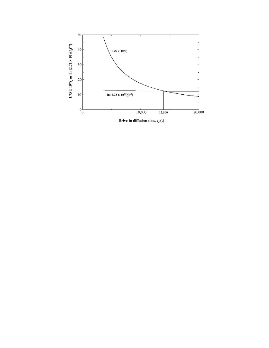
Excerpts from this work may be reproduced by instructors for distribution on a not-for-profit basis for testing or instructional purposes only to
students enrolled in courses for which the textbook has been adopted. Any other reproduction or translation of this work beyond that permitted
by Sections 107 or 108 of the 1976 United States Copyright Act without the permission of the copyright owner is unlawful.
As noted, the two curves intersect at about 13,900 s, which corresponds to t
d
= 3.86 h.
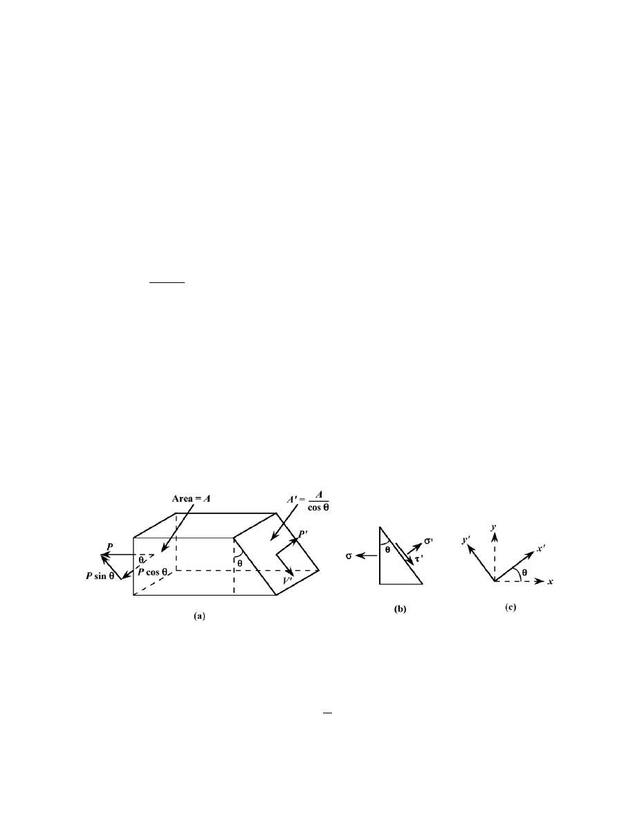
Excerpts from this work may be reproduced by instructors for distribution on a not-for-profit basis for testing or instructional purposes only to
students enrolled in courses for which the textbook has been adopted. Any other reproduction or translation of this work beyond that permitted
by Sections 107 or 108 of the 1976 United States Copyright Act without the permission of the copyright owner is unlawful.
CHAPTER 6
MECHANICAL PROPERTIES OF METALS
PROBLEM SOLUTIONS
Concepts of Stress and Strain
6.1 Using mechanics of materials principles (i.e., equations of mechanical equilibrium applied to a free-
body diagram), derive Equations 6.4a and 6.4b.
Solution
This problem asks that we derive Equations 6.4a and 6.4b, using mechanics of materials principles. In
Figure (a) below is shown a block element of material of cross-sectional area A that is subjected to a tensile force P.
Also represented is a plane that is oriented at an angle
θ referenced to the plane perpendicular to the tensile axis;
the area of this plane is A' = A/cos
θ. In addition, and the forces normal and parallel to this plane are labeled as P'
and V', respectively. Furthermore, on the left-hand side of this block element are shown force components that are
tangential and perpendicular to the inclined plane. In Figure (b) are shown the orientations of the applied stress
σ,
the normal stress to this plane
σ', as well as the shear stress τ' taken parallel to this inclined plane. In addition, two
coordinate axis systems in represented in Figure (c): the primed x and y axes are referenced to the inclined plane,
whereas the unprimed x axis is taken parallel to the applied stress.
Normal and shear stresses are defined by Equations 6.1 and 6.3, respectively. However, we now chose to
express these stresses in terms (i.e., general terms) of normal and shear forces (P and V) as
σ =
P
A

Excerpts from this work may be reproduced by instructors for distribution on a not-for-profit basis for testing or instructional purposes only to
students enrolled in courses for which the textbook has been adopted. Any other reproduction or translation of this work beyond that permitted
by Sections 107 or 108 of the 1976 United States Copyright Act without the permission of the copyright owner is unlawful.
τ =
V
A
For static equilibrium in the x' direction the following condition must be met:
F
∑
x'
= 0
which means that
PÕ
− P cos θ = 0
Or that
P' = P cos
θ
Now it is possible to write an expression for the stress
σ' in terms of P' and A' using the above expression and the
relationship between A and A' [Figure (a)]:
σ' =
PÕ
AÕ
=
P cos
θ
A
cos
θ
=
P
A
cos
2
θ
However, it is the case that P/A =
σ; and, after making this substitution into the above expression, we have
Equation 6.4a--that is
σ' = σ cos
2
θ
Now, for static equilibrium in the y' direction, it is necessary that
F
yÕ
∑
= 0
=
−VÕ+ P sinθ

Excerpts from this work may be reproduced by instructors for distribution on a not-for-profit basis for testing or instructional purposes only to
students enrolled in courses for which the textbook has been adopted. Any other reproduction or translation of this work beyond that permitted
by Sections 107 or 108 of the 1976 United States Copyright Act without the permission of the copyright owner is unlawful.
Or
V' = P sin
θ
We now write an expression for
τ' as
τÕ=
VÕ
AÕ
And, substitution of the above equation for V' and also the expression for A' gives
τ' =
VÕ
AÕ
=
P sin
θ
A
cos
θ
=
P
A
sin
θ cos θ
=
σ sinθ cos θ
which is just Equation 6.4b.
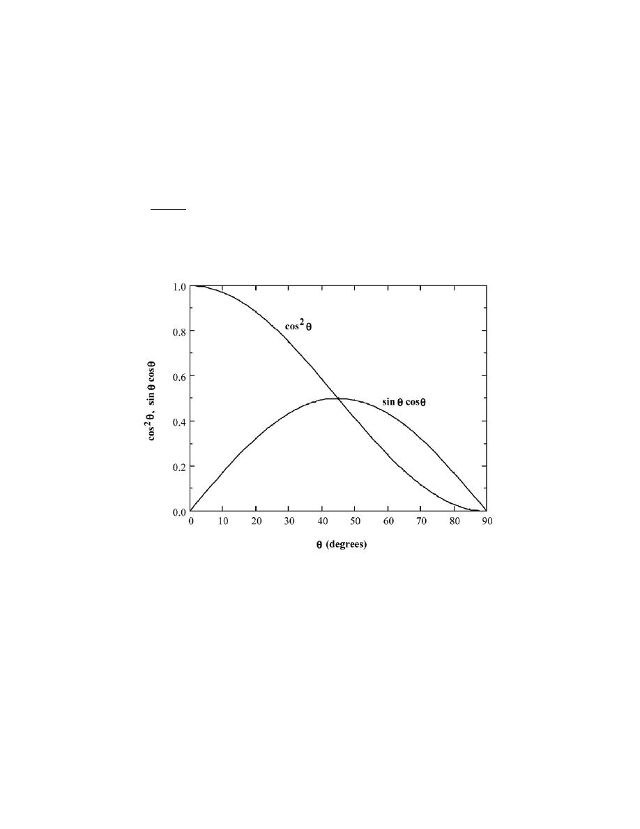
Excerpts from this work may be reproduced by instructors for distribution on a not-for-profit basis for testing or instructional purposes only to
students enrolled in courses for which the textbook has been adopted. Any other reproduction or translation of this work beyond that permitted
by Sections 107 or 108 of the 1976 United States Copyright Act without the permission of the copyright owner is unlawful.
6.2 (a) Equations 6.4a and 6.4b are expressions for normal (
σ′) and shear (τ′) stresses, respectively, as a
function of the applied tensile stress (σ) and the inclination angle of the plane on which these stresses are taken (θ
of Figure 6.4). Make a plot on which is presented the orientation parameters of these expressions (i.e., cos
2
θ and
sin θ cos θ) versus θ.
(b) From this plot, at what angle of inclination is the normal stress a maximum?
(c) Also, at what inclination angle is the shear stress a maximum?
Solution
(a) Below are plotted curves of cos
2
θ (for
σ' ) and sin θ cos θ (for τ') versus θ.
(b) The maximum normal stress occurs at an inclination angle of 0
°.
(c) The maximum shear stress occurs at an inclination angle of 45
°.

Excerpts from this work may be reproduced by instructors for distribution on a not-for-profit basis for testing or instructional purposes only to
students enrolled in courses for which the textbook has been adopted. Any other reproduction or translation of this work beyond that permitted
by Sections 107 or 108 of the 1976 United States Copyright Act without the permission of the copyright owner is unlawful.
Stress-Strain Behavior
6.3 A specimen of aluminum having a rectangular cross section 10 mm
× 12.7 mm (0.4 in. × 0.5 in.) is
pulled in tension with 35,500 N (8000 lb
f
) force, producing only elastic deformation. Calculate the resulting strain.
Solution
This problem calls for us to calculate the elastic strain that results for an aluminum specimen stressed in
tension. The cross-sectional area is just (10 mm)
× (12.7 mm) = 127 mm
2
(= 1.27
× 10
-4
m
2
= 0.20 in.
2
); also, the
elastic modulus for Al is given in Table 6.1 as 69 GPa (or 69
× 10
9
N/m
2
). Combining Equations 6.1 and 6.5 and
solving for the strain yields
ε =
σ
E
=
F
A
0
E
=
35, 500 N
(
1.27
× 10
−4
m
2
)(
69
× 10
9
N/m
2
)
= 4.1
× 10
-3

Excerpts from this work may be reproduced by instructors for distribution on a not-for-profit basis for testing or instructional purposes only to
students enrolled in courses for which the textbook has been adopted. Any other reproduction or translation of this work beyond that permitted
by Sections 107 or 108 of the 1976 United States Copyright Act without the permission of the copyright owner is unlawful.
6.4 A cylindrical specimen of a titanium alloy having an elastic modulus of 107 GPa (15.5
× 10
6
psi) and
an original diameter of 3.8 mm (0.15 in.) will experience only elastic deformation when a tensile load of 2000 N
(450 lb
f
) is applied. Compute the maximum length of the specimen before deformation if the maximum allowable
elongation is 0.42 mm (0.0165 in.).
Solution
We are asked to compute the maximum length of a cylindrical titanium alloy specimen (before
deformation) that is deformed elastically in tension. For a cylindrical specimen
A
0
=
π
d
0
2
2
where d
0
is the original diameter. Combining Equations 6.1, 6.2, and 6.5 and solving for l
0
leads to
l
0
=
∆l
ε
=
∆l
σ
E
Ê
=
∆l E
F
A
0
Ê
=
∆l Eπ
d
0
2
2
F
=
∆l Eπ d
0
2
4 F
=
(
0.42
× 10
−3
m
)
(
107
× 10
9
N / m
2
)
(
π)
(
3.8
× 10
−3
m
)
2
(4)(2000 N)
= 0.255 m = 255 mm (10.0 in.)

Excerpts from this work may be reproduced by instructors for distribution on a not-for-profit basis for testing or instructional purposes only to
students enrolled in courses for which the textbook has been adopted. Any other reproduction or translation of this work beyond that permitted
by Sections 107 or 108 of the 1976 United States Copyright Act without the permission of the copyright owner is unlawful.
6.5 A steel bar 100 mm (4.0 in.) long and having a square cross section 20 mm (0.8 in.) on an edge is
pulled in tension with a load of 89,000 N (20,000 lb
f
), and experiences an elongation of 0.10 mm (4.0
× 10
-3
in.).
Assuming that the deformation is entirely elastic, calculate the elastic modulus of the steel.
Solution
This problem asks us to compute the elastic modulus of steel. For a square cross-section, A
0
=
b
0
2
, where
b
0
is the edge length. Combining Equations 6.1, 6.2, and 6.5 and solving for E, leads to
E =
σ
ε
=
F
A
0
∆l
l
0
=
Fl
0
b
0
2
∆ l
=
(89, 000 N)
(
100
× 10
−3
m
)
(
20
× 10
−3
m
)
2
(
0.10
× 10
−3
m
)
= 223
× 10
9
N/m
2
= 223 GPa (31.3
× 10
6
psi)

Excerpts from this work may be reproduced by instructors for distribution on a not-for-profit basis for testing or instructional purposes only to
students enrolled in courses for which the textbook has been adopted. Any other reproduction or translation of this work beyond that permitted
by Sections 107 or 108 of the 1976 United States Copyright Act without the permission of the copyright owner is unlawful.
6.6 Consider a cylindrical titanium wire 3.0 mm (0.12 in.) in diameter and 2.5
× 10
4
mm (1000 in.) long.
Calculate its elongation when a load of 500 N (112 lb
f
) is applied. Assume that the deformation is totally elastic.
Solution
In order to compute the elongation of the Ti wire when the 500 N load is applied we must employ
Equation
s 6.1, 6.2, and 6.5. Solving for ∆l and realizing that for Ti, E = 107 GPa (15.5 × 10
6
psi) (Table 6.1),
∆l = l
0
ε = l
0
σ
E
=
l
0
F
EA
0
=
l
0
F
E
π
d
0
2
2
=
4l
0
F
E
πd
0
2
=
(4)(25 m)(500 N)
(
107
× 10
9
N/m
2
)
(
π )
(
3
× 10
−3
m
)
2
= 0.0165 m = 16.5 mm (0.65 in.)

Excerpts from this work may be reproduced by instructors for distribution on a not-for-profit basis for testing or instructional purposes only to
students enrolled in courses for which the textbook has been adopted. Any other reproduction or translation of this work beyond that permitted
by Sections 107 or 108 of the 1976 United States Copyright Act without the permission of the copyright owner is unlawful.
6.7 For a bronze alloy, the stress at which plastic deformation begins is 275 MPa (40,000 psi), and the
modulus of elasticity is 115 GPa (16.7
× 10
6
psi).
(a) What is the maximum load that may be applied to a specimen with a cross-sectional area of 325 mm
2
(0.5 in.
2
) without plastic deformation?
(b) If the original specimen length is 115 mm (4.5 in.), what is the maximum length to which it may be
stretched without causing plastic deformation?
Solution
(a) This portion of the problem calls for a determination of the maximum load that can be applied without
plastic deformation (F
y
). Taking the yield strength to be 275 MPa, and employment of Equation 6.1 leads to
F
y
=
σ
y
A
0
=
(
275
× 10
6
N/m
2
)(
325
× 10
-6
m
2
)
= 89,375 N (20,000 lb
f
)
(b) The maximum length to which the sample may be deformed without plastic deformation is determined
from Equations 6.2 and 6.5 as
l
i
= l
0
1
+
σ
E
= (115 mm) 1
+
275 MPa
115
× 10
3
MPa
= 115.28 mm (4.51 in.)
Excerpts from this work may be reproduced by instructors for distribution on a not-for-profit basis for testing or instructional purposes only to
students enrolled in courses for which the textbook has been adopted. Any other reproduction or translation of this work beyond that permitted
by Sections 107 or 108 of the 1976 United States Copyright Act without the permission of the copyright owner is unlawful.
6.8 A cylindrical rod of copper (E = 110 GPa, 16
× 10
6
psi) having a yield strength of 240 MPa (35,000
psi) is to be subjected to a load of 6660 N (1500 lb
f
). If the length of the rod is 380 mm (15.0 in.), what must be the
diameter to allow an elongation of 0.50 mm (0.020 in.)?
Solution
This problem asks us to compute the diameter of a cylindrical specimen of copper in order to allow an
elongation of 0.50 mm. Employing Equations 6.1, 6.2, and 6.5, assuming that deformation is entirely elastic
σ =
F
A
0
=
F
π
d
0
2
4
= E
∆ l
l
0
Or, solving for d
0
d
0
=
4 l
0
F
π E ∆l
=
(4)
(
380
× 10
−3
m
)
(6660 N)
(
π)
(
110
× 10
9
N / m
2
)(
0.50
× 10
−3
m
)
= 7.65
× 10
-3
m = 7.65 mm (0.30 in.)

Excerpts from this work may be reproduced by instructors for distribution on a not-for-profit basis for testing or instructional purposes only to
students enrolled in courses for which the textbook has been adopted. Any other reproduction or translation of this work beyond that permitted
by Sections 107 or 108 of the 1976 United States Copyright Act without the permission of the copyright owner is unlawful.
6.9 Compute the elastic moduli for the following metal alloys, whose stress-strain behaviors may be
observed in the “Tensile Tests” module of Virtual Materials Science and Engineering (VMSE): (a) titanium, (b)
tempered steel, (c) aluminum, and (d) carbon steel. How do these values compare with those presented in Table 6.1
for the same metals?
Solution
The elastic modulus is the slope in the linear elastic region (Equation 6.10) as
E =
∆ σ
∆ ε
=
σ
2
− σ
1
ε
2
− ε
1
Since stress-strain curves for all of the metals/alloys pass through the origin, we make take
σ
1
= 0 and
ε
1
= 0.
Determinations of
σ
2
and
ε
2
are possible by moving the cursor to some arbitrary point in the linear region of the
curve and then reading corresponding values in the “Stress” and “Strain” windows that are located below the plot.
(a) For the titanium alloy, we selected
σ
2
= 404.2 MPa with its corresponding
ε
2
= 0.0038. Therefore,
E =
σ
2
− σ
1
ε
2
− ε
1
=
404.2 MPa
− 0 MPa
0.0038
− 0
= 106,400 MPa = 106.4 GPa
The elastic modulus for titanium given in Table 6.1 is 107 GPa, which is in very good agreement with this
value.
(b) For the tempered steel, we selected
σ
2
= 962.2 MPa with its corresponding
ε
2
= 0.0047. Therefore,
E =
σ
2
− σ
1
ε
2
− ε
1
=
962.2 MPa
− 0 MPa
0.0047
− 0
= 204,700 MPa = 204.7 GPa

Excerpts from this work may be reproduced by instructors for distribution on a not-for-profit basis for testing or instructional purposes only to
students enrolled in courses for which the textbook has been adopted. Any other reproduction or translation of this work beyond that permitted
by Sections 107 or 108 of the 1976 United States Copyright Act without the permission of the copyright owner is unlawful.
The elastic modulus for steel given in Table 6.1 is 207 GPa, which is in reasonably good agreement with
this value.
(c) For the aluminum, we selected
σ
2
= 145.1 MPa with its corresponding
ε
2
= 0.0021. Therefore,
E =
σ
2
− σ
1
ε
2
− ε
1
=
145.1 MPa
− 0 MPa
0.0021
− 0
= 69,100 MPa = 69.1 GPa
The elastic modulus for aluminum given in Table 6.1 is 69 GPa, which is in excellent agreement with this
value.
(d) For the carbon steel, we selected
σ
2
= 129 MPa with its corresponding
ε
2
= 0.0006. Therefore,
E =
σ
2
− σ
1
ε
2
− ε
1
=
129 MPa
− 0 MPa
0.0006
− 0
= 215,000 MPa = 215 GPa
The elastic modulus for steel given in Table 6.1 is 207 GPa, which is in reasonable agreement with this
value.

Excerpts from this work may be reproduced by instructors for distribution on a not-for-profit basis for testing or instructional purposes only to
students enrolled in courses for which the textbook has been adopted. Any other reproduction or translation of this work beyond that permitted
by Sections 107 or 108 of the 1976 United States Copyright Act without the permission of the copyright owner is unlawful.
6.10 Consider a cylindrical specimen of a steel alloy (Figure 6.21) 10.0 mm (0.39 in.) in diameter and 75
mm (3.0 in.) long that is pulled in tension. Determine its elongation when a load of 20,000 N (4,500 lb
f
) is applied.
Solution
This problem asks that we calculate the elongation ∆l of a specimen of steel the stress-strain behavior of
which is shown in Figure 6.21. First it becomes necessary to compute the stress when a load of 20,000 N is applied
using Equation 6.1 as
σ =
F
A
0
=
F
π
d
0
2
2
=
20, 000 N
π
10.0
× 10
−3
m
2
2
= 255 MPa (37, 700 psi)
Referring to Figure 6.21, at this stress level we are in the elastic region on the stress-strain curve, which corresponds
to a strain of 0.0012. Now, utilization of Equation 6.2 to compute the value of
∆l
∆ l = εl
0
= (0.0012)(75 mm) = 0.090 mm (0.0036 in.)
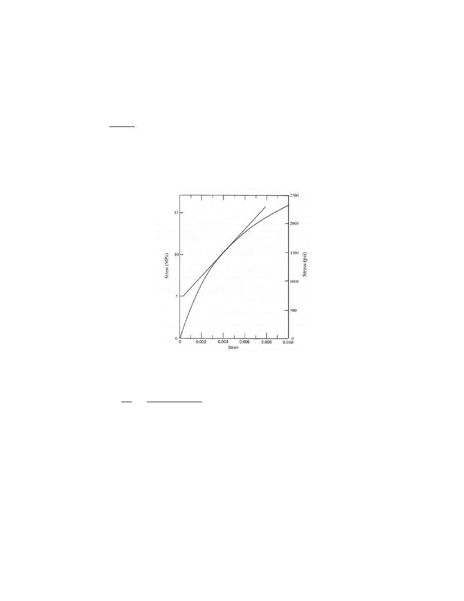
Excerpts from this work may be reproduced by instructors for distribution on a not-for-profit basis for testing or instructional purposes only to
students enrolled in courses for which the textbook has been adopted. Any other reproduction or translation of this work beyond that permitted
by Sections 107 or 108 of the 1976 United States Copyright Act without the permission of the copyright owner is unlawful.
6.11 Figure 6.22 shows, for a gray cast iron, the tensile engineering stress–strain curve in the elastic
region. Determine (a) the tangent modulus at 10.3 MPa (1500 psi), and (b) the secant modulus taken to 6.9 MPa
(1000 psi).
Solution
(a) This portion of the problem asks that the tangent modulus be determined for the gray cast iron, the
stress-strain behavior of which is shown in Figure 6.22. In the figure below is shown a tangent draw on the curve at
a stress of 10.3 MPa (1500 psi).
The slope of this line (i.e., ∆σ/∆ε), the tangent modulus, is computed as follows:
∆σ
∆ε
=
15 MPa
− 5 MPa
0.0074
− 0.0003
= 1410 MPa = 1.41 GPa (2.04
× 10
5
psi)
(b) The secant modulus taken from the origin is calculated by taking the slope of a secant drawn from the
origin through the stress-strain curve at 6.9 MPa (1,000 psi). This secant is drawn on the curve shown below:
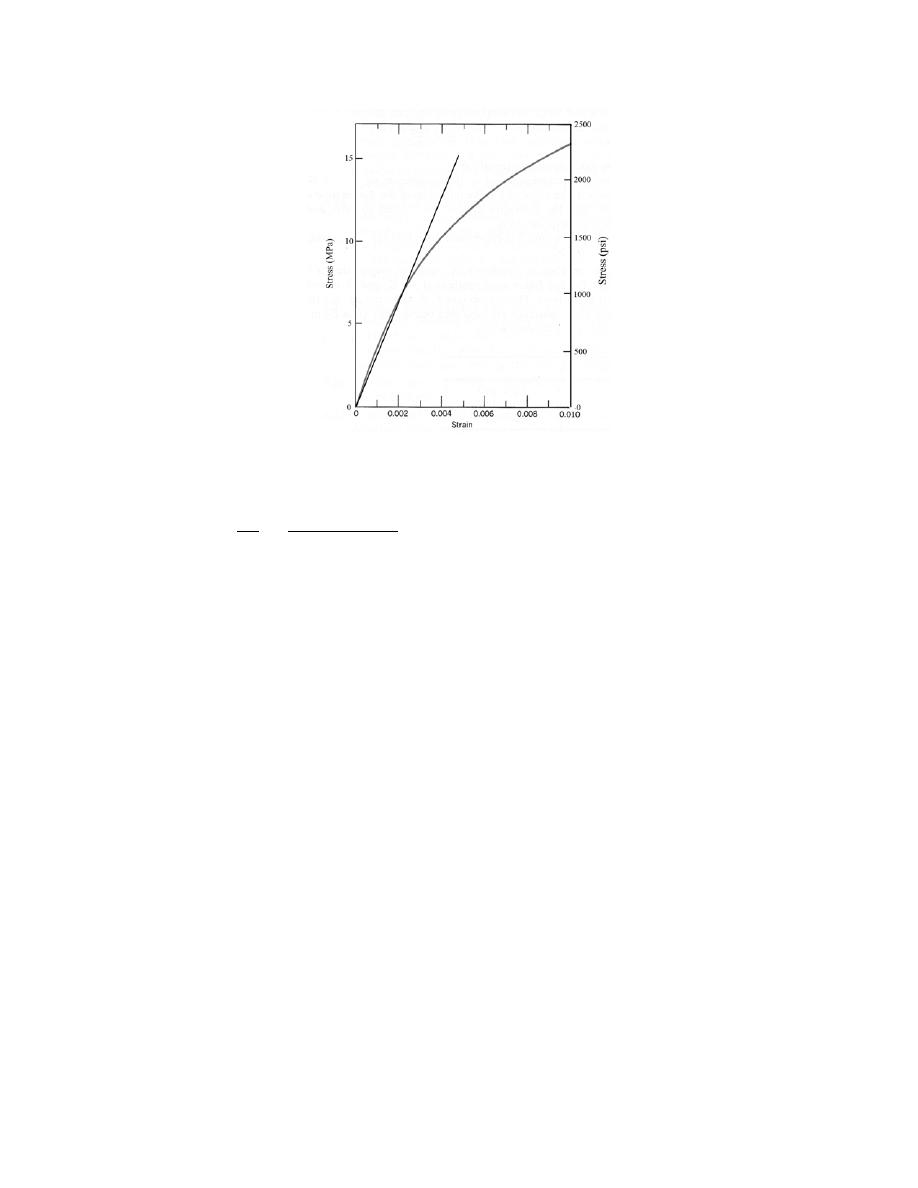
Excerpts from this work may be reproduced by instructors for distribution on a not-for-profit basis for testing or instructional purposes only to
students enrolled in courses for which the textbook has been adopted. Any other reproduction or translation of this work beyond that permitted
by Sections 107 or 108 of the 1976 United States Copyright Act without the permission of the copyright owner is unlawful.
The slope of this line (i.e., ∆σ/∆ε), the secant modulus, is computed as follows:
∆σ
∆ε
=
15 MPa
− 0 MPa
0.0047
− 0
= 3190 MPa = 3.19 GPa (4.63
× 10
5
psi)
Excerpts from this work may be reproduced by instructors for distribution on a not-for-profit basis for testing or instructional purposes only to
students enrolled in courses for which the textbook has been adopted. Any other reproduction or translation of this work beyond that permitted
by Sections 107 or 108 of the 1976 United States Copyright Act without the permission of the copyright owner is unlawful.
6.12 As noted in Section 3.15, for single crystals of some substances, the physical properties are
anisotropic; that is, they are dependent on crystallographic direction. One such property is the modulus of
elasticity. For cubic single crystals, the modulus of elasticity in a general [uvw] direction, E
uvw
, is described by the
relationship
1
E
uvw
=
1
E
100
− 3
1
E
100
−
1
E
111
α
2
β
2
+ β
2
γ
2
+ γ
2
α
2
(
)
where
E
100
and
E
111
are the moduli of elasticity in [100] and [111] directions, respectively;
α, β, and γ are the
cosines of the angles between [uvw] and the respective [100], [010], and [001] directions. Verify that the
E
〈110〉
values for aluminum, copper, and iron in Table 3.3 are correct.
Solution
We are asked, using the equation given in the problem statement, to verify that the modulus of elasticity
values along [110] directions given in Table 3.3 for aluminum, copper, and iron are correct. The
α, β, and γ
parameters in the equation correspond, respectively, to the cosines of the angles between the [110] direction and
[100], [010] and [001] directions. Since these angles are 45
°, 45°, and 90°, the values of α, β, and γ are 0.707,
0.707, and 0, respectively. Thus, the given equation takes the form
1
E
<110>
=
1
E
<100>
− 3
1
E
<100>
−
1
E
<111>
(0.707)
2
(0.707)
2
+ (0.707)
2
(0)
2
+ (0)
2
(0.707)
2
[
]
=
1
E
<100>
− (0.75)
1
E
<100>
−
1
E
<111>
Utilizing the values of E
<100>
and E
<111>
from Table 3.3 for Al
1
E
<110>
=
1
63.7 GPa
− (0.75)
1
63.7 GPa
−
1
76.1 GPa
Which leads to, E
<110>
= 72.6 GPa, the value cited in the table.

Excerpts from this work may be reproduced by instructors for distribution on a not-for-profit basis for testing or instructional purposes only to
students enrolled in courses for which the textbook has been adopted. Any other reproduction or translation of this work beyond that permitted
by Sections 107 or 108 of the 1976 United States Copyright Act without the permission of the copyright owner is unlawful.
For Cu,
1
E
<110>
=
1
66.7 GPa
− (0.75)
1
66.7 GPa
−
1
191.1 GPa
Thus, E
<110>
= 130.3 GPa, which is also the value cited in the table.
Similarly, for Fe
1
E
<110>
=
1
125.0 GPa
− (0.75)
1
125.0 GPa
−
1
272.7 GPa
And E
<110>
= 210.5 GPa, which is also the value given in the table.

Excerpts from this work may be reproduced by instructors for distribution on a not-for-profit basis for testing or instructional purposes only to
students enrolled in courses for which the textbook has been adopted. Any other reproduction or translation of this work beyond that permitted
by Sections 107 or 108 of the 1976 United States Copyright Act without the permission of the copyright owner is unlawful.
6.13 In Section 2.6 it was noted that the net bonding energy E
N
between two isolated positive and negative
ions is a function of interionic distance r as follows:
E
N
= −
A
r
+
B
r
n
(6.25)
where A, B, and n are constants for the particular ion pair. Equation 6.25 is also valid for the bonding energy
between adjacent ions in solid materials. The modulus of elasticity E is proportional to the slope of the interionic
force–separation curve at the equilibrium interionic separation; that is,
E
∝
dF
dr
r
o
Derive an expression for the dependence of the modulus of elasticity on these A, B, and n parameters (for the two-
ion system) using the following procedure:
1. Establish a relationship for the force F as a function of r, realizing that
F
=
dE
N
dr
2. Now take the derivative dF/dr.
3. Develop an expression for r
0
, the equilibrium separation. Since r
0
corresponds to the value of r at the
minimum of the E
N
-versus-r curve (Figure 2.8b), take the derivative dE
N
/dr, set it equal to zero, and solve for r,
which corresponds to r
0
.
4. Finally, substitute this expression for r
0
into the relationship obtained by taking dF/dr.
Solution
This problem asks that we derive an expression for the dependence of the modulus of elasticity, E, on the
parameters A, B, and n in Equation 6.25. It is first necessary to take dE
N
/dr in order to obtain an expression for the
force F; this is accomplished as follows:
F =
dE
N
d r
=
d
−
A
r
d r
+
d
B
r
n
d r
=
A
r
2
−
nB
r
(n
+1)

Excerpts from this work may be reproduced by instructors for distribution on a not-for-profit basis for testing or instructional purposes only to
students enrolled in courses for which the textbook has been adopted. Any other reproduction or translation of this work beyond that permitted
by Sections 107 or 108 of the 1976 United States Copyright Act without the permission of the copyright owner is unlawful.
The second step is to set this dE
N
/dr expression equal to zero and then solve for r (= r0). The algebra for this
procedure is carried out in Problem 2.14, with the result that
r
0
=
A
nB
1/(1
− n)
Next it becomes necessary to take the derivative of the force (dF/dr), which is accomplished as follows:
dF
dr
=
d
A
r
2
dr
+
d
−
nB
r
(n
+1)
dr
=
−
2 A
r
3
+
(n)(n
+ 1)B
r
(n
+2)
Now, substitution of the above expression for r
0
into this equation yields
dF
dr
r
0
=
−
2 A
A
nB
3/(1
−n)
+
(n)(n
+ 1) B
A
nB
(n
+2)/(1−n)
which is the expression to which the modulus of elasticity is proportional.

Excerpts from this work may be reproduced by instructors for distribution on a not-for-profit basis for testing or instructional purposes only to
students enrolled in courses for which the textbook has been adopted. Any other reproduction or translation of this work beyond that permitted
by Sections 107 or 108 of the 1976 United States Copyright Act without the permission of the copyright owner is unlawful.
6.14 Using the solution to Problem 6.13, rank the magnitudes of the moduli of elasticity for the following
hypothetical X, Y, and Z materials from the greatest to the least. The appropriate A, B, and n parameters (Equation
6.25) for these three materials are tabulated below; they yield E
N
in units of electron volts and r in nanometers:
Material
A
B
n
X
2.5
2.0 × 10
–5
8
Y
2.3
8.0 × 10
–6
10.5
Z
3.0
1.5 × 10
–5
9
Solution
This problem asks that we rank the magnitudes of the moduli of elasticity of the three hypothetical metals
X, Y, and Z. From Problem 6.13, it was shown for materials in which the bonding energy is dependent on the
interatomic distance r according to Equation 6.25, that the modulus of elasticity E is proportional to
E
∝ −
2 A
A
nB
3/(1
−n)
+
(n)(n
+ 1) B
A
nB
(n
+2)/(1−n)
For metal X, A = 2.5, B = 2.0
× 10
-5
, and n = 8. Therefore,
E
∝ −
(2)(2.5)
2.5
(8)
(
2
× 10
−5
)
3/(1
− 8)
+
(8)(8
+1)
(
2
× 10
−5
)
2.5
(8)
(
2
× 10
−5
)
(8
+ 2)/(1 − 8)
= 1097
For metal Y, A = 2.3, B = 8
× 10
-6
, and n = 10.5. Hence
E
∝ −
(2)(2.3)
2.3
(10.5)
(
8
× 10
−6
)
3/(1
− 10.5)
+
(10.5)(10.5
+ 1)
(
8
× 10
−6
)
2.3
(10.5)
(
8
× 10
−6
)
(10.5
+ 2)/(1 − 10.5)
= 551
And, for metal Z, A = 3.0, B = 1.5
× 10
-5
, and n = 9. Thus

Excerpts from this work may be reproduced by instructors for distribution on a not-for-profit basis for testing or instructional purposes only to
students enrolled in courses for which the textbook has been adopted. Any other reproduction or translation of this work beyond that permitted
by Sections 107 or 108 of the 1976 United States Copyright Act without the permission of the copyright owner is unlawful.
E
∝ −
(2)(3.0)
3.0
(9)
(
1.5
× 10
−5
)
3/(1
− 9)
+
(9)(9
+ 1)
(
1.5
× 10
−5
)
3.0
(9)
(
1.5
× 10
−5
)
(9
+ 2)/(1 − 9)
= 1024
Therefore, metal X has the highest modulus of elasticity.

Excerpts from this work may be reproduced by instructors for distribution on a not-for-profit basis for testing or instructional purposes only to
students enrolled in courses for which the textbook has been adopted. Any other reproduction or translation of this work beyond that permitted
by Sections 107 or 108 of the 1976 United States Copyright Act without the permission of the copyright owner is unlawful.
Elastic Properties of Materials
6.15 A cylindrical specimen of aluminum having a diameter of 19 mm (0.75 in.) and length of 200 mm (8.0
in.) is deformed elastically in tension with a force of 48,800 N (11,000 lb
f
). Using the data contained in Table 6.1,
determine the following:
(a) The amount by which this specimen will elongate in the direction of the applied stress.
(b) The change in diameter of the specimen. Will the diameter increase or decrease?
Solution
(a) We are asked, in this portion of the problem, to determine the elongation of a cylindrical specimen of
aluminum. Combining Equations 6.1, 6.2, and 6.5, leads to
σ = Eε
F
π
d
0
2
4
= E
∆ l
l
0
Or, solving for
∆l (and realizing that E = 69 GPa, Table 6.1), yields
∆ l =
4 F l
0
π d
0
2
E
=
(4)(48,800 N)
(
200
× 10
−3
m
)
(
π)
(
19
× 10
−3
m
)
2
(
69
× 10
9
N / m
2
)
= 5 × 10
-4
m = 0.50 mm (0.02 in.)
(b) We are now called upon to determine the change in diameter,
∆d. Using Equation 6.8
ν = −
ε
x
ε
z
=
−
∆d /d
0
∆ l /l
0
From Table 6.1, for aluminum,
ν
= 0.33. Now, solving the above expression for ∆d yields
∆d = −
ν ∆l d
0
l
0
=
−
(0.33)(0.50 mm)(19 mm)
200 mm
= –1.6
× 10
-2
mm (–6.2
× 10
-4
in.)

Excerpts from this work may be reproduced by instructors for distribution on a not-for-profit basis for testing or instructional purposes only to
students enrolled in courses for which the textbook has been adopted. Any other reproduction or translation of this work beyond that permitted
by Sections 107 or 108 of the 1976 United States Copyright Act without the permission of the copyright owner is unlawful.
The diameter will decrease.

Excerpts from this work may be reproduced by instructors for distribution on a not-for-profit basis for testing or instructional purposes only to
students enrolled in courses for which the textbook has been adopted. Any other reproduction or translation of this work beyond that permitted
by Sections 107 or 108 of the 1976 United States Copyright Act without the permission of the copyright owner is unlawful.
6.16 A cylindrical bar of steel 10 mm (0.4 in.) in diameter is to be deformed elastically by application of a
force along the bar axis. Using the data in Table 6.1, determine the force that will produce an elastic reduction of 3
× 10
-3
mm (1.2
× 10
-4
in.) in the diameter.
Solution
This problem asks that we calculate the force necessary to produce a reduction in diameter of 3
× 10
-3
mm
for a cylindrical bar of steel. For a cylindrical specimen, the cross-sectional area is equal to
A
0
=
π d
0
2
4
Now, combining Equations 6.1 and 6.5 leads to
σ =
F
A
0
=
F
πd
0
2
4
= Eε
z
And, since from Equation 6.8
ε
z
= −
ε
x
ν
= −
∆d
d
0
ν
= −
∆d
νd
0
Substitution of this equation into the above expression gives
F
πd
0
2
4
= E −
∆d
νd
0
And, solving for F leads to
F =
−
d
0
∆d π E
4
ν
From Table 6.1, for steel,
ν = 0.30 and E = 207 GPa. Thus,

Excerpts from this work may be reproduced by instructors for distribution on a not-for-profit basis for testing or instructional purposes only to
students enrolled in courses for which the textbook has been adopted. Any other reproduction or translation of this work beyond that permitted
by Sections 107 or 108 of the 1976 United States Copyright Act without the permission of the copyright owner is unlawful.
F =
−
(
10
× 10
−3
m
)(
− 3.0 × 10
−6
m
)
(
π)
(
207
× 10
9
N / m
2
)
(4)(0.30)
= 16,250 N (3770 lb
f
)

Excerpts from this work may be reproduced by instructors for distribution on a not-for-profit basis for testing or instructional purposes only to
students enrolled in courses for which the textbook has been adopted. Any other reproduction or translation of this work beyond that permitted
by Sections 107 or 108 of the 1976 United States Copyright Act without the permission of the copyright owner is unlawful.
6.17 A cylindrical specimen of some alloy 8 mm (0.31 in.) in diameter is stressed elastically in tension. A
force of 15,700 N (3530 lb
f
) produces a reduction in specimen diameter of 5
× 10
-3
mm (2
× 10
-4
in.). Compute
Poisson's ratio for this material if its modulus of elasticity is 140 GPa (20.3
× 10
6
psi).
Solution
This problem asks that we compute Poisson's ratio for the metal alloy. From Equations 6.5 and 6.1
ε
z
=
σ
E
=
F
A
0
E
=
F
π
d
0
2
2
E
=
4 F
π d
0
2
E
Since the transverse strain
ε
x
is just
ε
x
=
∆d
d
0
and Poisson's ratio is defined by Equation 6.8, then
ν = −
ε
x
ε
z
=
−
∆d /d
0
4 F
π d
0
2
E
=
−
d
0
∆d π E
4 F
=
−
(
8
× 10
−3
m
)(
−5 × 10
−6
m
)
(
π)
(
140
× 10
9
N / m
2
)
(4)(15, 700 N)
= 0.280

Excerpts from this work may be reproduced by instructors for distribution on a not-for-profit basis for testing or instructional purposes only to
students enrolled in courses for which the textbook has been adopted. Any other reproduction or translation of this work beyond that permitted
by Sections 107 or 108 of the 1976 United States Copyright Act without the permission of the copyright owner is unlawful.
6.18 A cylindrical specimen of a hypothetical metal alloy is stressed in compression. If its original and
final diameters are 20.000 and 20.025 mm, respectively, and its final length is 74.96 mm, compute its original
length if the deformation is totally elastic. The elastic and shear moduli for this alloy are 105 GPa and 39.7 GPa,
respectively.
Solution
This problem asks that we compute the original length of a cylindrical specimen that is stressed in
compression. It is first convenient to compute the lateral strain
ε
x
as
ε
x
=
∆d
d
0
=
20.025 mm
− 20.000 mm
20.000 mm
= 1.25
× 10
-3
In order to determine the longitudinal strain
ε
z
we need Poisson's ratio, which may be computed using Equation 6.9;
solving for
ν yields
ν =
E
2 G
− 1 =
105
× 10
3
MPa
(2)
(
39.7
× 10
3
MPa
)
− 1 = 0.322
Now
ε
z
may be computed from Equation 6.8 as
ε
z
=
−
ε
x
ν
=
−
1.25
× 10
−3
0.322
=
− 3.88 × 10
-3
Now solving for l
0
using Equation 6.2
l
0
=
l
i
1
+ ε
z
=
74.96 mm
1
− 3.88 × 10
−3
= 75.25 mm

Excerpts from this work may be reproduced by instructors for distribution on a not-for-profit basis for testing or instructional purposes only to
students enrolled in courses for which the textbook has been adopted. Any other reproduction or translation of this work beyond that permitted
by Sections 107 or 108 of the 1976 United States Copyright Act without the permission of the copyright owner is unlawful.
6.19 Consider a cylindrical specimen of some hypothetical metal alloy that has a diameter of 8.0 mm (0.31
in.). A tensile force of 1000 N (225 lb
f
) produces an elastic reduction in diameter of 2.8
× 10
-4
mm (1.10
× 10
-5
in.).
Compute the modulus of elasticity for this alloy, given that Poisson's ratio is 0.30.
Solution
This problem asks that we calculate the modulus of elasticity of a metal that is stressed in tension.
Combining Equations 6.5 and 6.1 leads to
E =
σ
ε
z
=
F
A
0
ε
z
=
F
ε
z
π
d
0
2
2
=
4 F
ε
z
π d
0
2
From the definition of Poisson's ratio, (Equation 6.8) and realizing that for the transverse strain,
ε
x
=
∆d
d
0
ε
z
=
−
ε
x
ν
=
−
∆d
d
0
ν
Therefore, substitution of this expression for
ε
z
into the above equation yields
E =
4 F
ε
z
π d
0
2
=
4 F
ν
π d
0
∆d
=
(4)(1000 N)(0.30)
π
(
8
× 10
−3
m
)(
2.8
× 10
−7
m
)
= 1.705
× 10
11
Pa = 170.5 GPa (24.7
× 10
6
psi)

Excerpts from this work may be reproduced by instructors for distribution on a not-for-profit basis for testing or instructional purposes only to
students enrolled in courses for which the textbook has been adopted. Any other reproduction or translation of this work beyond that permitted
by Sections 107 or 108 of the 1976 United States Copyright Act without the permission of the copyright owner is unlawful.
6.20 A brass alloy is known to have a yield strength of 275 MPa (40,000 psi), a tensile strength of 380
MPa (55,000 psi), and an elastic modulus of 103 GPa (15.0
× 10
6
psi). A cylindrical specimen of this alloy 12.7
mm (0.50 in.) in diameter and 250 mm (10.0 in.) long is stressed in tension and found to elongate 7.6 mm (0.30 in.).
On the basis of the information given, is it possible to compute the magnitude of the load that is necessary to
produce this change in length? If so, calculate the load. If not, explain why.
Solution
We are asked to ascertain whether or not it is possible to compute, for brass, the magnitude of the load
necessary to produce an elongation of 7.6 mm (0.30 in.). It is first necessary to compute the strain at yielding from
the yield strength and the elastic modulus, and then the strain experienced by the test specimen. Then, if
ε(test) < ε(yield)
deformation is elastic, and the load may be computed using Equations 6.1 and 6.5. However, if
ε(test) > ε(yield)
computation of the load is not possible inasmuch as deformation is plastic and we have neither a stress-strain plot
nor a mathematical expression relating plastic stress and strain. We compute these two strain values as
ε(test) =
∆l
l
0
=
7.6 mm
250 mm
= 0.03
and
ε(yield) =
σ
y
E
=
275 MPa
103
× 10
3
MPa
= 0.0027
Therefore, computation of the load is not possible since
ε(test) > ε(yield).
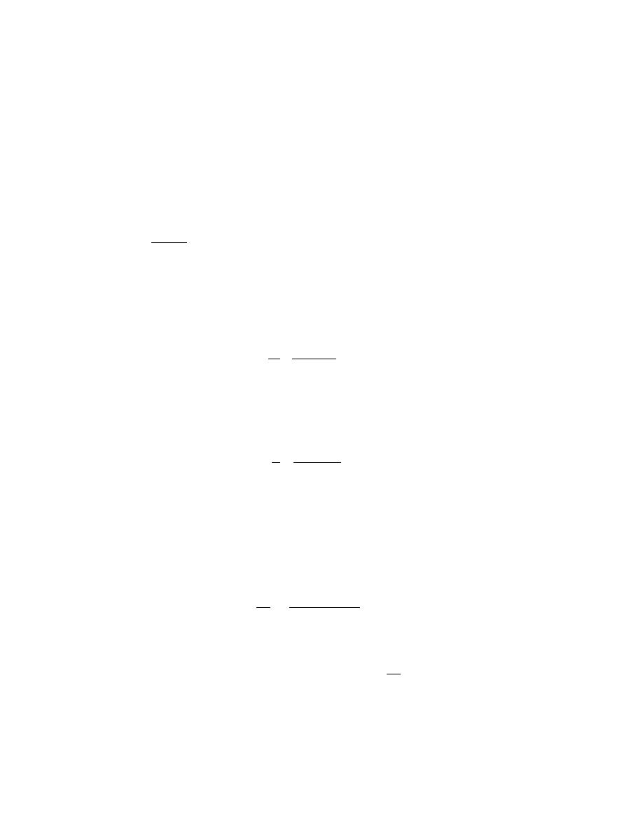
Excerpts from this work may be reproduced by instructors for distribution on a not-for-profit basis for testing or instructional purposes only to
students enrolled in courses for which the textbook has been adopted. Any other reproduction or translation of this work beyond that permitted
by Sections 107 or 108 of the 1976 United States Copyright Act without the permission of the copyright owner is unlawful.
6.21 A cylindrical metal specimen 12.7 mm (0.5 in.) in diameter and 250 mm (10 in.) long is to be
subjected to a tensile stress of 28 MPa (4000 psi); at this stress level the resulting deformation will be totally
elastic.
(a) If the elongation must be less than 0.080 mm (3.2
× 10
-3
in.), which of the metals in Table 6.1 are
suitable candidates? Why?
(b) If, in addition, the maximum permissible diameter decrease is 1.2
× 10
-3
mm (4.7
× 10
-5
in.) when the
tensile stress of 28 MPa is applied, which of the metals that satisfy the criterion in part (a) are suitable candidates?
Why?
Solution
(a) This part of the problem asks that we ascertain which of the metals in Table 6.1 experience an
elongation of less than 0.080 mm when subjected to a tensile
stress of 28 MPa. The maximum strain that may be
sustained, (using Equation 6.2) is just
ε =
∆l
l
0
=
0.080 mm
250 mm
= 3.2
× 10
-4
Since the stress level is given (50 MPa), using Equation 6.5 it is possible to compute the minimum modulus of
elasticity which is required to yield this minimum strain. Hence
E =
σ
ε
=
28 MPa
3.2
× 10
−4
= 87.5 GPa
Which means that those metals with moduli of elasticity greater than this value are acceptable candidates—namely,
brass, Cu, Ni, steel, Ti and W.
(b) This portion of the problem further stipulates that the maximum permissible diameter decrease is 1.2
×
10
-3
mm when the tensile stress of 28 MPa is applied. This translates into a maximum lateral strain
ε
x
(max) as
ε
x (max)
=
∆d
d
0
=
−1.2 × 10
−3
mm
12.7 mm
=
− 9.45 × 10
-5
But, since the specimen contracts in this lateral direction, and we are concerned that this strain be less than 9.45
×
10
-5
, then the criterion for this part of the problem may be stipulated as
−
∆d
d
0
< 9.45 × 10
-5.
Now, Poisson’s ratio is defined by Equation 6.8 as

Excerpts from this work may be reproduced by instructors for distribution on a not-for-profit basis for testing or instructional purposes only to
students enrolled in courses for which the textbook has been adopted. Any other reproduction or translation of this work beyond that permitted
by Sections 107 or 108 of the 1976 United States Copyright Act without the permission of the copyright owner is unlawful.
ν = −
ε
x
ε
z
For each of the metal alloys let us consider a possible lateral strain,
ε
x
=
∆d
d
0
. Furthermore, since the deformation is
elastic, then, from Equation 6.5, the longitudinal strain,
ε
z
is equal to
ε
z
=
σ
E
Substituting these expressions for
ε
x
and
ε
z
into the definition of Poisson’s ratio we have
ν = −
ε
x
ε
z
=−
∆d
d
0
σ
E
which leads to the following:
−
∆d
d
0
=
ν σ
E
Using values for
ν and E found in Table 6.1 for the six metal alloys that satisfy the criterion for part (a), and for σ =
28 MPa, we are able to compute a
−
∆d
d
0
for each alloy as follows:
−
∆d
d
0
(brass)
=
(0.34)(28
× 10
6
N / m
2
)
97
× 10
9
N / m
2
= 9.81 × 10
−5
−
∆d
d
0
(copper)
=
(0.34)(28
× 10
6
N / m
2
)
110
× 10
9
N / m
2
= 8.65 × 10
−5
−
∆d
d
0
(titanium)
=
(0.34)(28
× 10
6
N / m
2
)
107
× 10
9
N / m
2
= 8.90 × 10
−5
−
∆d
d
0
(nickel)
=
(0.31)(28
× 10
6
N / m
2
)
207
× 10
9
N / m
2
= 4.19 × 10
−5
−
∆d
d
0
(steel)
=
(0.30)(28
× 10
6
N / m
2
)
207
× 10
9
N / m
2
= 4.06 × 10
−5

Excerpts from this work may be reproduced by instructors for distribution on a not-for-profit basis for testing or instructional purposes only to
students enrolled in courses for which the textbook has been adopted. Any other reproduction or translation of this work beyond that permitted
by Sections 107 or 108 of the 1976 United States Copyright Act without the permission of the copyright owner is unlawful.
−
∆d
d
0
(tungsten)
=
(0.28)(28
× 10
6
N / m
2
)
407
× 10
9
N / m
2
= 1.93 × 10
−5
Thus, of the above six alloys, only brass will have a negative transverse strain that is greater than 9.45
× 10
-5
. This
means that the following alloys satisfy the criteria for both parts (a) and (b) of the problem: copper, titanium,
nickel, steel, and tungsten.

Excerpts from this work may be reproduced by instructors for distribution on a not-for-profit basis for testing or instructional purposes only to
students enrolled in courses for which the textbook has been adopted. Any other reproduction or translation of this work beyond that permitted
by Sections 107 or 108 of the 1976 United States Copyright Act without the permission of the copyright owner is unlawful.
6.22 Consider the brass alloy for which the stress-strain behavior is shown in Figure 6.12. A cylindrical
specimen of this material 6 mm (0.24 in.) in diameter and 50 mm (2 in.) long is pulled in tension with a force of
5000 N (1125 lb
f
). If it is known that this alloy has a Poisson's ratio of 0.30, compute: (a) the specimen elongation,
and (b) the reduction in specimen diameter.
Solution
(a) This portion of the problem asks that we compute the elongation of the brass specimen. The first
calculation necessary is that of the applied stress using Equation 6.1, as
σ =
F
A
0
=
F
π
d
0
2
2
=
5000 N
π
6
× 10
−3
m
2
2
= 177
× 10
6
N/m
2
= 177 MPa (25,000 psi)
From the stress-strain plot in Figure 6.12, this stress corresponds to a strain of about 2.0
× 10
-3
. From the definition
of strain, Equation 6.2
∆l = εl
0
=
(
2.0
× 10
-3
)
(50 mm) = 0.10 mm (4
× 10
-3
in.)
(b) In order to determine the reduction in diameter ∆d, it is necessary to use Equation 6.8 and the
definition of lateral strain (i.e.,
ε
x
= ∆d/d
0
) as follows
∆d = d
0
ε
x
=
− d
0
ν ε
z
=
− (6 mm)(0.30)
(
2.0
× 10
-3
)
= –3.6
× 10
-3
mm (–1.4
× 10
-4
in.)

Excerpts from this work may be reproduced by instructors for distribution on a not-for-profit basis for testing or instructional purposes only to
students enrolled in courses for which the textbook has been adopted. Any other reproduction or translation of this work beyond that permitted
by Sections 107 or 108 of the 1976 United States Copyright Act without the permission of the copyright owner is unlawful.
6.23 A cylindrical rod 100 mm long and having a diameter of 10.0 mm is to be deformed using a tensile
load of 27,500 N. It must not experience either plastic deformation or a diameter reduction of more than 7.5
× 10
-3
mm. Of the materials listed as follows, which are possible candidates? Justify your choice(s).
Material
Modulus of Elasticity
(GPa)
Yield Strength
(MPa)
Poisson’s Ratio
Aluminum alloy
70
200
0.33
Brass alloy
101
300
0.34
Steel alloy
207
400
0.30
Titanium alloy
107
650
0.34
Solution
This problem asks that we assess the four alloys relative to the two criteria presented. The first criterion is
that the material not experience plastic deformation when the tensile load of 27,500 N is applied; this means that
the stress corresponding to this load not exceed the yield strength of the material. Upon computing the stress
σ =
F
A
0
=
F
π
d
0
2
2
=
27, 500 N
π
10
× 10
−3
m
2
2
= 350
× 10
6
N/m
2
= 350 MPa
Of the alloys listed, the Ti and steel alloys have yield strengths greater than 350 MPa.
Relative to the second criterion (i.e., that
∆d be less than 7.5 × 10
-3
mm), it is necessary to calculate the
change in diameter ∆d for these three alloys. From Equation 6.8
ν = −
ε
x
ε
z
=
−
∆d
d
0
σ
E
= −
E
∆d
σ d
0
Now, solving for ∆d from this expression,
∆d = −
ν σ d
0
E
For the steel alloy

Excerpts from this work may be reproduced by instructors for distribution on a not-for-profit basis for testing or instructional purposes only to
students enrolled in courses for which the textbook has been adopted. Any other reproduction or translation of this work beyond that permitted
by Sections 107 or 108 of the 1976 United States Copyright Act without the permission of the copyright owner is unlawful.
∆d = −
(0.30)(350 MPa)(10 mm)
207
× 10
3
MPa
=
− 5.1 × 10
-3
mm
Therefore, the steel is a candidate.
For the Ti alloy
∆d = −
(0.34)(350 MPa)(10 mm)
107
× 10
3
MPa
=
−11.1 × 10
-3
mm
Hence, the titanium alloy is not a candidate.

Excerpts from this work may be reproduced by instructors for distribution on a not-for-profit basis for testing or instructional purposes only to
students enrolled in courses for which the textbook has been adopted. Any other reproduction or translation of this work beyond that permitted
by Sections 107 or 108 of the 1976 United States Copyright Act without the permission of the copyright owner is unlawful.
6.24 A cylindrical rod 380 mm (15.0 in.) long, having a diameter of 10.0 mm (0.40 in.), is to be subjected
to a tensile load. If the rod is to experience neither plastic deformation nor an elongation of more than 0.9 mm
(0.035 in.) when the applied load is 24,500 N (5500 lb
f
), which of the four metals or alloys listed below are possible
candidates? Justify your choice(s).
Material
Modulus of Elasticity
(GPa)
Yield Strength
(MPa)
Tensile Strength
(MPa)
Aluminum alloy
70
255
420
Brass alloy
100
345
420
Copper
110
250
290
Steel alloy
207
450
550
Solution
This problem asks that we ascertain which of four metal alloys will not (1) experience plastic deformation,
and (2) elongate more than 0.9 mm when a tensile load of 24,500 N is applied. It is first necessary to compute the
stress using Equation 6.1; a material to be used for this application must necessarily have a yield strength greater
than this value. Thus,
σ =
F
A
0
=
24, 500 N
π
10.0
× 10
−3
m
2
2
= 312 MPa
Of the metal alloys listed, only brass and steel have yield strengths greater than this stress.
Next, we must compute the elongation produced in both brass and steel using Equations 6.2 and 6.5 in
order to determine whether or not this elongation is less than 0.9 mm. For brass
∆l =
σ l
0
E
=
(312 MPa)(380 mm)
100
× 10
3
MPa
= 1.19 mm
Thus, brass is not a candidate. However, for steel
∆l =
σ l
0
E
=
(312 MPa)(380 mm)
207
× 10
3
MPa
= 0.57 mm
Therefore, of these four alloys, only steel satisfies the stipulated criteria.

Excerpts from this work may be reproduced by instructors for distribution on a not-for-profit basis for testing or instructional purposes only to
students enrolled in courses for which the textbook has been adopted. Any other reproduction or translation of this work beyond that permitted
by Sections 107 or 108 of the 1976 United States Copyright Act without the permission of the copyright owner is unlawful.
Tensile Properties
6.25 Figure 6.21 shows the tensile engineering stress–strain behavior for a steel alloy.
(a) What is the modulus of elasticity?
(b) What is the proportional limit?
(c) What is the yield strength at a strain offset of 0.002?
(d) What is the tensile strength?
Solution
Using the stress-strain plot for a steel alloy (Figure 6.21), we are asked to determine several of its
mechanical characteristics.
(a) The elastic modulus is just the slope of the initial linear portion of the curve; or, from the inset and
using Equation 6.10
E =
σ
2
− σ
1
ε
2
− ε
1
=
(200
− 0) MPa
(
0.0010
− 0
)
= 200
× 10
3
MPa = 200 GPa ( 29
× 10
6
psi)
The value given in Table 6.1 is 207 GPa.
(b) The proportional limit is the stress level at which linearity of the stress-strain curve ends, which is
approximately 300 MPa (43,500 psi).
(c) The 0.002 strain offset line intersects the stress-strain curve at approximately 400 MPa (58,000 psi).
(d) The tensile strength (the maximum on the curve) is approximately 515 MPa (74,700 psi).

Excerpts from this work may be reproduced by instructors for distribution on a not-for-profit basis for testing or instructional purposes only to
students enrolled in courses for which the textbook has been adopted. Any other reproduction or translation of this work beyond that permitted
by Sections 107 or 108 of the 1976 United States Copyright Act without the permission of the copyright owner is unlawful.
6.26 A cylindrical specimen of a brass alloy having a length of 60 mm (2.36 in.) must elongate only 10.8
mm (0.425 in.) when a tensile load of 50,000 N (11,240 lb
f
) is applied. Under these circumstances, what must be
the radius of the specimen? Consider this brass alloy to have the stress-strain behavior shown in Figure 6.12.
Solution
We are asked to calculate the radius of a cylindrical brass specimen in order to produce an elongation of
10.8 mm when a load of 50,000 N is applied. It first becomes necessary to compute the strain corresponding to this
elongation using Equation 6.2 as
ε =
∆l
l
0
=
10.8 mm
60 mm
= 0.18
From Figure 6.12, a stress of 420 MPa (61,000 psi) corresponds to this strain. Since for a cylindrical specimen,
stress, force, and initial radius r
0
are related as
σ =
F
π r
0
2
then
r
0
=
F
π σ
=
50, 000 N
π
(
420
× 10
6
N / m
2
)
= 0.0062 m = 6.2 mm (0.24 in.)

Excerpts from this work may be reproduced by instructors for distribution on a not-for-profit basis for testing or instructional purposes only to
students enrolled in courses for which the textbook has been adopted. Any other reproduction or translation of this work beyond that permitted
by Sections 107 or 108 of the 1976 United States Copyright Act without the permission of the copyright owner is unlawful.
6.27 A load of 85,000 N (19,100 lb
f
) is applied to a cylindrical specimen of a steel alloy (displaying the
stress–strain behavior shown in Figure 6.21) that has a cross-sectional diameter of 15 mm (0.59 in.).
(a) Will the specimen experience elastic and/or plastic deformation? Why?
(b) If the original specimen length is 250 mm (10 in.), how much will it increase in length when this load is
applied?
Solution
This problem asks us to determine the deformation characteristics of a steel specimen, the stress-strain
behavior for which is shown in Figure 6.21.
(a) In order to ascertain whether the deformation is elastic or plastic, we must first compute the stress, then
locate it on the stress-strain curve, and, finally, note whether this point is on the elastic or plastic region. Thus, from
Equation 6.1
σ =
F
A
0
=
85, 000 N
π
15
× 10
−3
m
2
2
= 481
× 10
6
N/m
2
= 481 MPa (69, 900 psi)
The 481 MPa point is beyond the linear portion of the curve, and, therefore, the deformation will be both elastic and
plastic.
(b) This portion of the problem asks us to compute the increase in specimen length. From the stress-strain
curve, the strain at 481 MPa is approximately 0.0135. Thus, from Equation 6.2
∆l = εl
0
= (0.0135)(250 mm) = 3.4 mm (0.135 in.)

Excerpts from this work may be reproduced by instructors for distribution on a not-for-profit basis for testing or instructional purposes only to
students enrolled in courses for which the textbook has been adopted. Any other reproduction or translation of this work beyond that permitted
by Sections 107 or 108 of the 1976 United States Copyright Act without the permission of the copyright owner is unlawful.
6.28 A bar of a steel alloy that exhibits the stress-strain behavior shown in Figure 6.21 is subjected to a
tensile load; the specimen is 300 mm (12 in.) long, and of square cross section 4.5 mm (0.175 in.) on a side.
(a) Compute the magnitude of the load necessary to produce an elongation of 0.45 mm (0.018 in.).
(b) What will be the deformation after the load has been released?
Solution
(a) We are asked to compute the magnitude of the load necessary to produce an elongation of 0.45 mm for
the steel displaying the stress-strain behavior shown in Figure 6.21. First, calculate the strain, and then the
corresponding stress from the plot.
ε =
∆l
l
0
=
0.45 mm
300 mm
=1.5
× 10
−3
This is near the end of the elastic region; from the inset of Figure 6.21, this corresponds to a stress of about 300
MPa (43,500 psi). Now, from Equation 6.1
F =
σA
0
=
σb
2
in which b is the cross-section side length. Thus,
F =
(
300
× 10
6
N/m
2
)
(
4.5
× 10
-3
m
)
2
= 6075 N (1366 lb
f
)
(b) After the load is released there will be no deformation since the material was strained only elastically.

Excerpts from this work may be reproduced by instructors for distribution on a not-for-profit basis for testing or instructional purposes only to
students enrolled in courses for which the textbook has been adopted. Any other reproduction or translation of this work beyond that permitted
by Sections 107 or 108 of the 1976 United States Copyright Act without the permission of the copyright owner is unlawful.
6.29 A cylindrical specimen of aluminum having a diameter of 0.505 in. (12.8 mm) and a gauge length of
2.000 in. (50.800 mm) is pulled in tension. Use the load–elongation characteristics tabulated below to complete
parts (a) through (f).
Load
Length
N
lb
f
mm
in.
0
0
50.800
2.000
7,330
1,650
50.851
2.002
15,100
3,400
50.902
2.004
23,100
5,200
50.952
2.006
30,400
6,850
51.003
2.008
34,400
7,750
51.054
2.010
38,400
8,650
51.308
2.020
41,300
9,300
51.816
2.040
44,800
10,100
52.832
2.080
46,200
10,400
53.848
2.120
47,300
10,650
54.864
2.160
47,500
10,700
55.880
2.200
46,100
10,400
56.896
2.240
44,800
10,100
57.658
2.270
42,600
9,600
58.420
2.300
36,400
8,200
59.182
2.330
Fracture
(a) Plot the data as engineering stress versus engineering strain.
(b) Compute the modulus of elasticity.
(c) Determine the yield strength at a strain offset of 0.002.
(d) Determine the tensile strength of this alloy.
(e) What is the approximate ductility, in percent elongation?
(f) Compute the modulus of resilience.
Solution
This problem calls for us to make a stress-strain plot for aluminum, given its tensile load-length data, and
then to determine some of its mechanical characteristics.
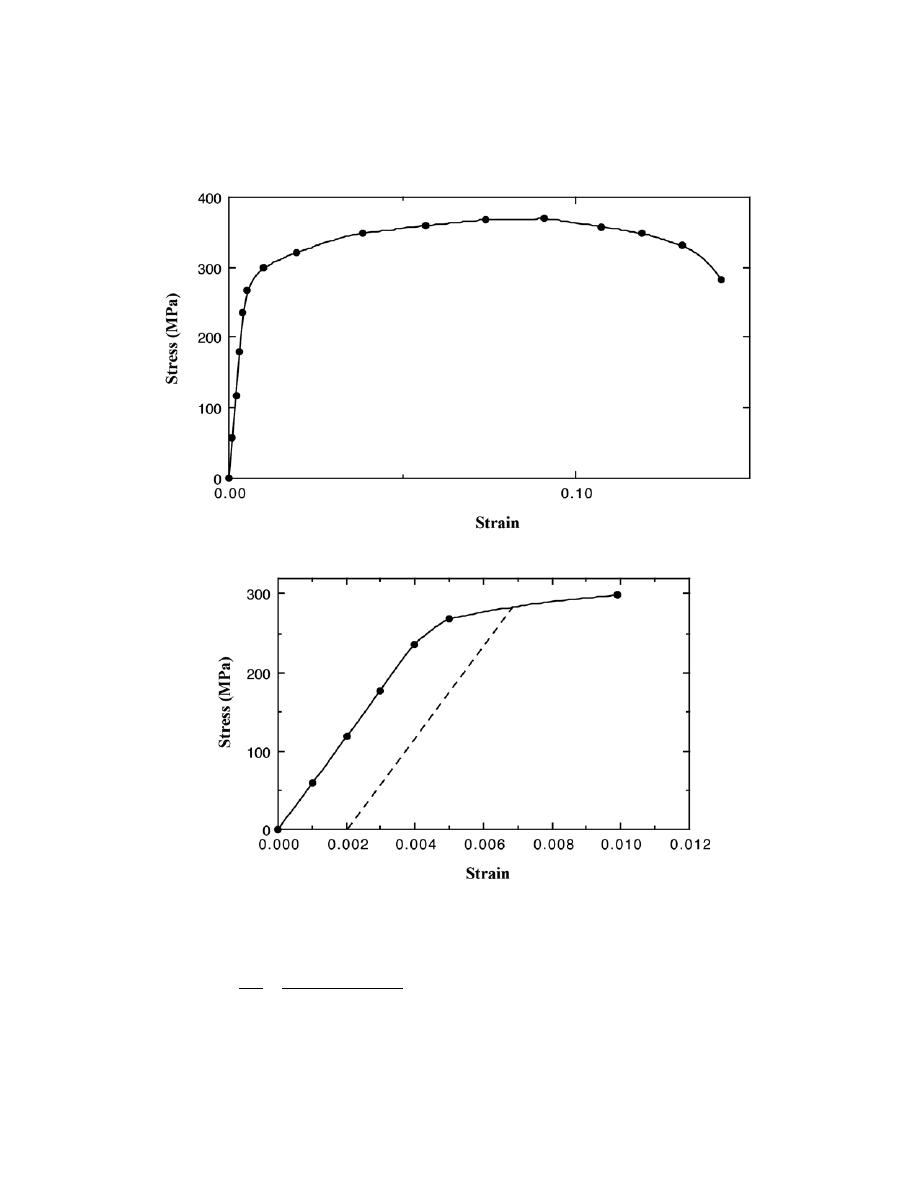
Excerpts from this work may be reproduced by instructors for distribution on a not-for-profit basis for testing or instructional purposes only to
students enrolled in courses for which the textbook has been adopted. Any other reproduction or translation of this work beyond that permitted
by Sections 107 or 108 of the 1976 United States Copyright Act without the permission of the copyright owner is unlawful.
(a) The data are plotted below on two plots: the first corresponds to the entire stress-strain curve, while
for the second, the curve extends to just beyond the elastic region of deformation.
(b) The elastic modulus is the slope in the linear elastic region (Equation 6.10) as
E =
∆ σ
∆ ε
=
200 MPa
− 0 MPa
0.0032
− 0
= 62.5
× 10
3
MPa = 62.5 GPa (9.1
× 10
6
psi)

Excerpts from this work may be reproduced by instructors for distribution on a not-for-profit basis for testing or instructional purposes only to
students enrolled in courses for which the textbook has been adopted. Any other reproduction or translation of this work beyond that permitted
by Sections 107 or 108 of the 1976 United States Copyright Act without the permission of the copyright owner is unlawful.
(c) For the yield strength, the 0.002 strain offset line is drawn dashed. It intersects the stress-strain curve
at approximately 285 MPa (41,000 psi ).
(d) The tensile strength is approximately 370 MPa (54,000 psi), corresponding to the maximum stress on
the complete stress-strain plot.
(e) The ductility, in percent elongation, is just the plastic strain at fracture, multiplied by one-hundred.
The total fracture strain at fracture is 0.165; subtracting out the elastic strain (which is about 0.005) leaves a plastic
strain of 0.160. Thus, the ductility is about 16%EL.
(f) From Equation 6.14, the modulus of resilience is just
U
r
=
σ
y
2
2E
which, using data computed above gives a value of
U
r
=
(285 MPa)
2
(2)
(
62.5
× 10
3
MPa
)
= 0.65 MN/m
2
= 0.65 × 10
6
N/m
2
= 6.5 × 10
5
J/m
3
(
93.8 in. - lb
f
/in.
3
)

Excerpts from this work may be reproduced by instructors for distribution on a not-for-profit basis for testing or instructional purposes only to
students enrolled in courses for which the textbook has been adopted. Any other reproduction or translation of this work beyond that permitted
by Sections 107 or 108 of the 1976 United States Copyright Act without the permission of the copyright owner is unlawful.
6.30 A specimen of ductile cast iron having a rectangular cross section of dimensions 4.8 mm
× 15.9 mm
(3/16 in.
× 5/8 in.) is deformed in tension. Using the load-elongation data tabulated below, complete problems (a)
through (f).
Load
Length
N
lb
f
mm
in.
0
0
75.000
2.953
4,740
1,065
75.025
2.954
9,140
2,055
75.050
2.955
12,920
2,900
75.075
2.956
16,540
3,720
75.113
2.957
18,300
4,110
75.150
2.959
20,170
4,530
75.225
2.962
22,900
5,145
75.375
2.968
25,070
5,635
75.525
2.973
26,800
6,025
75.750
2.982
28,640
6,440
76.500
3.012
30,240
6,800
78.000
3.071
31,100
7,000
79.500
3.130
31,280
7,030
81.000
3.189
30,820
6,930
82.500
3.248
29,180
6,560
84.000
3.307
27,190
6,110
85.500
3.366
24,140
5,430
87.000
3.425
18,970
4,265
88.725
3.493
Fracture
(a) Plot the data as engineering stress versus engineering strain.
(b) Compute the modulus of elasticity.
(c) Determine the yield strength at a strain offset of 0.002.
(d) Determine the tensile strength of this alloy.
(e) Compute the modulus of resilience.
(f) What is the ductility, in percent elongation?
Solution
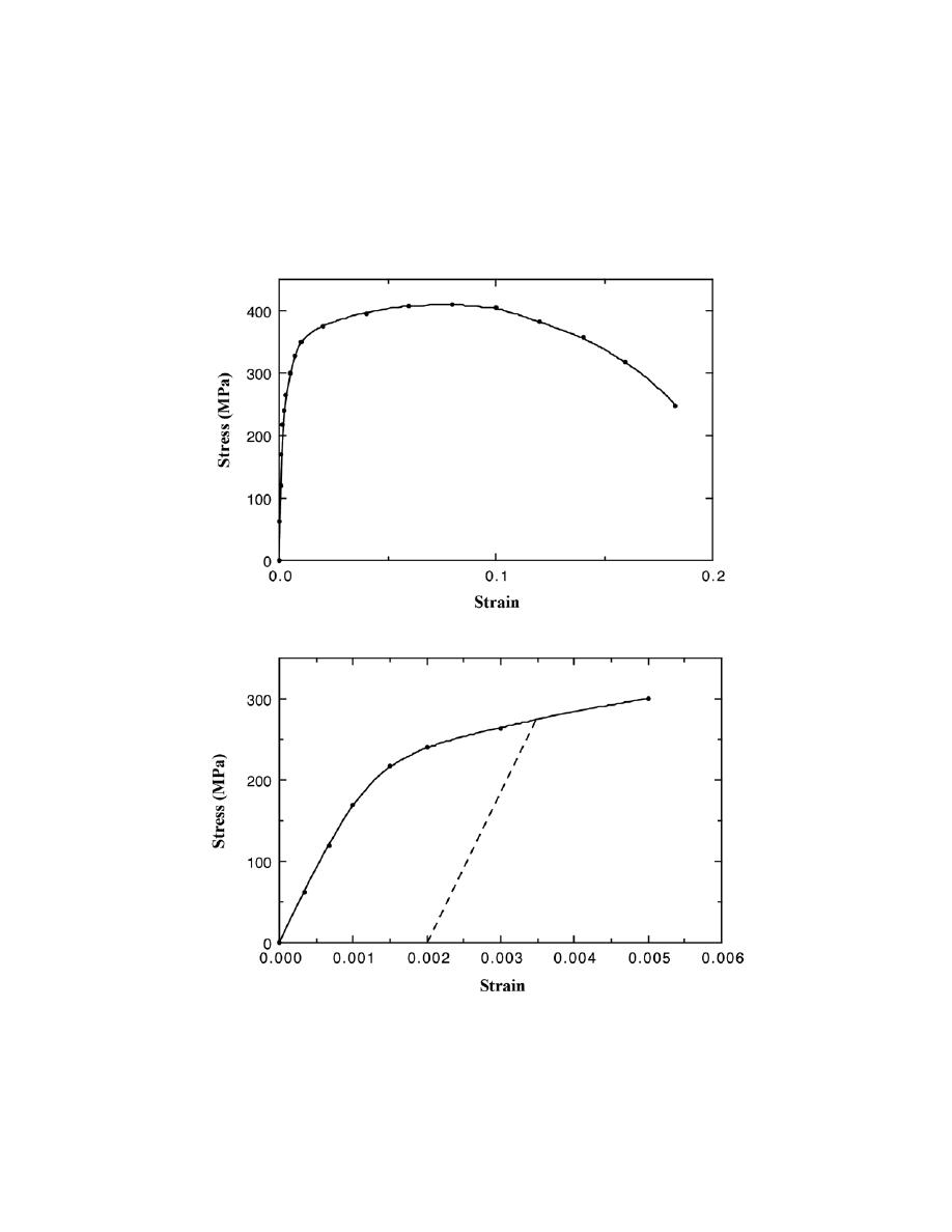
Excerpts from this work may be reproduced by instructors for distribution on a not-for-profit basis for testing or instructional purposes only to
students enrolled in courses for which the textbook has been adopted. Any other reproduction or translation of this work beyond that permitted
by Sections 107 or 108 of the 1976 United States Copyright Act without the permission of the copyright owner is unlawful.
This problem calls for us to make a stress-strain plot for a ductile cast iron, given its tensile load-length
data, and then to determine some of its mechanical characteristics.
(a) The data are plotted below on two plots: the first corresponds to the entire stress-strain curve, while
for the second, the curve extends just beyond the elastic region of deformation.
(b) The elastic modulus is the slope in the linear elastic region (Equation 6.10) as

Excerpts from this work may be reproduced by instructors for distribution on a not-for-profit basis for testing or instructional purposes only to
students enrolled in courses for which the textbook has been adopted. Any other reproduction or translation of this work beyond that permitted
by Sections 107 or 108 of the 1976 United States Copyright Act without the permission of the copyright owner is unlawful.
E =
∆ σ
∆ ε
=
100 MPa
− 0 MPa
0.0005
− 0
= 200 × 10
3
MPa = 200 GPa (29
× 10
6
psi)
(c) For the yield strength, the 0.002 strain offset line is drawn dashed. It intersects the stress-strain curve
at approximately 280 MPa (40,500 psi).
(d) The tensile strength is approximately 410 MPa (59,500 psi), corresponding to the maximum stress on
the complete stress-strain plot.
(e) From Equation 6.14, the modulus of resilience is just
U
r
=
σ
y
2
2 E
which, using data computed above, yields a value of
U
r
=
(
280
× 10
6
N / m
2
)
2
(2)
(
200
× 10
9
N / m
2
)
= 1.96
× 10
5
J/m
3
(
28.3 in. - lb
f
/in.
3
)
(f) The ductility, in percent elongation, is just the plastic strain at fracture, multiplied by one-hundred. The
total fracture strain at fracture is 0.185; subtracting out the elastic strain (which is about 0.001) leaves a plastic
strain of 0.184. Thus, the ductility is about 18.4%EL.

Excerpts from this work may be reproduced by instructors for distribution on a not-for-profit basis for testing or instructional purposes only to
students enrolled in courses for which the textbook has been adopted. Any other reproduction or translation of this work beyond that permitted
by Sections 107 or 108 of the 1976 United States Copyright Act without the permission of the copyright owner is unlawful.
6.31 For the titanium alloy, whose stress strain behavior may be observed in the “Tensile Tests” module
of Virtual Materials Science and Engineering (VMSE), determine the following:
(a) the approximate yield strength (0.002 strain offset),
(b) the tensile strength, and
(c) the approximate ductility, in percent elongation.
How do these values compare with those for the two Ti-6Al-4V alloys presented in Table B.4 of Appendix B?
Solution
(a) It is possible to do a screen capture and then print out the entire stress-strain curve for the Ti alloy.
The intersection of a straight line parallel to the initial linear region of the curve and offset at a strain of 0.002 with
this curve is at approximately 720 MPa.
(b) The maximum reading in the stress window located below the plot as the curser point is dragged along
the stress-strain curve is 1000 MPa, the value of the tensile strength.
(c) The approximate percent elongation corresponds to the strain at fracture multiplied by 100 (i.e., 12%)
minus the maximum elastic strain (i.e., value of strain at which the linearity of the curve ends multiplied by 100—in
this case about 0.5%); this gives a value of about 11.5%EL.
From Table B.4 in Appendix B, yield strength, tensile strength, and percent elongation values for the
anneal Ti-6Al-4V are 830 MPa, 900 MPa, and 14%EL, while for the solution heat treated and aged alloy, the
corresponding values are 1103 MPa, 1172 MPa, and 10%EL. Thus, tensile strength and percent elongation values
for the VMSE alloy are slightly lower than for the annealed material in Table B.4 (720 vs 830 MPa, and 11.5 vs. 14
%EL), whereas the tensile strength is slightly higher (1000 vs. 900 MPa).

Excerpts from this work may be reproduced by instructors for distribution on a not-for-profit basis for testing or instructional purposes only to
students enrolled in courses for which the textbook has been adopted. Any other reproduction or translation of this work beyond that permitted
by Sections 107 or 108 of the 1976 United States Copyright Act without the permission of the copyright owner is unlawful.
6.32 For the tempered steel alloy, whose stress strain behavior may be observed in the “Tensile Tests”
module of Virtual Materials Science and Engineering (VMSE), determine the following:
(a) the approximate yield strength (0.002 strain offset),
(b) the tensile strength, and
(c) the approximate ductility, in percent elongation.
How do these values compare with those for the oil-quenched and tempered 4140 and 4340 steel alloys presented in
Table B.4 of Appendix B?
Solution
(a) It is possible to do a screen capture and then print out the entire stress-strain curve for the tempered
steel alloy. The intersection of a straight line parallel to the initial linear region of the curve and offset at a strain of
0.002 with this curve is at approximately 1430 MPa.
(b) The maximum reading in the stress window located below the plot as the curser point is dragged along
the stress-strain curve is 1656 MPa, the value of the tensile strength.
(c) The approximate percent elongation corresponds to the strain at fracture multiplied by 100 (i.e., 14.8%)
minus the maximum elastic strain (i.e., value of strain at which the linearity of the curve ends multiplied by 100—in
this case about 0.8%); this gives a value of about 14.0%EL.
For the oil-quenched and tempered 4140 and 4340 steel alloys, yield strength values presented in Table B.4
of Appendix B are 1570 MPa and 1620 MPa, respectively; these values are somewhat larger than the 1430 MPa for
the tempered steel alloy of VMSE. Tensile strength values for these 4140 and 4340 alloys are, respectively 1720
MPa and 1760 MPa (compared to 1656 MPa for the VMSE steel). And, finally, the respective ductilities for the
4140 and 4340 alloys are 11.5%EL and 12%EL, which are slightly lower than the 14%EL value for the VMSE steel.

Excerpts from this work may be reproduced by instructors for distribution on a not-for-profit basis for testing or instructional purposes only to
students enrolled in courses for which the textbook has been adopted. Any other reproduction or translation of this work beyond that permitted
by Sections 107 or 108 of the 1976 United States Copyright Act without the permission of the copyright owner is unlawful.
6.33 For the aluminum alloy, whose stress strain behavior may be observed in the “Tensile Tests” module
of Virtual Materials Science and Engineering (VMSE), determine the following:
(a) the approximate yield strength (0.002 strain offset),
(b) the tensile strength, and
(c) the approximate ductility, in percent elongation.
How do these values compare with those for the 2024 aluminum alloy (T351 temper) presented in Table B.4 of
Appendix B?
Solution
(a) It is possible to do a screen capture and then print out the entire stress-strain curve for the aluminum
alloy. The intersection of a straight line parallel to the initial linear region of the curve and offset at a strain of 0.002
with this curve is at approximately 300 MPa.
(b) The maximum reading in the stress window located below the plot as the curser point is dragged along
the stress-strain curve is 484 MPa, the value of the tensile strength.
(c) The approximate percent elongation corresponds to the strain at fracture multiplied by 100 (i.e., 22.4%)
minus the maximum elastic strain (i.e., value of strain at which the linearity of the curve ends multiplied by 100—in
this case about 0.5%); this gives a value of about 21.9%EL.
For the 2024 aluminum alloy (T351 temper), the yield strength value presented in Table B.4 of Appendix
B is 325, which is slightly larger than the 300 MPa for the aluminum alloy of VMSE. The tensile strength value for
the 2024-T351 is 470 MPa (compared to 484 MPa for the VMSE alloy). And, finally, the ductility for 2024-T351 is
20%EL, which is about the same as for the VMSE aluminum (21.9%EL).

Excerpts from this work may be reproduced by instructors for distribution on a not-for-profit basis for testing or instructional purposes only to
students enrolled in courses for which the textbook has been adopted. Any other reproduction or translation of this work beyond that permitted
by Sections 107 or 108 of the 1976 United States Copyright Act without the permission of the copyright owner is unlawful.
6.34 For the (plain) carbon steel alloy, whose stress strain behavior may be observed in the “Tensile
Tests” module of Virtual Materials Science and Engineering (VMSE), determine the following:
(a) the approximate yield strength,
(b) the tensile strength, and
(c) the approximate ductility, in percent elongation.
Solution
(a) It is possible to do a screen capture and then print out the entire stress-strain curve for the plain carbon
steel alloy. Inasmuch as the stress-strain curve displays the yield point phenomenon, we take the yield strength as
the lower yield point, which, for this steel, is about 225 MPa.
(b) The maximum reading in the stress window located below the plot as the curser point is dragged along
the stress-strain curve is 274 MPa, the value of the tensile strength.
(c) The approximate percent elongation corresponds to the strain at fracture multiplied by 100 (i.e., 43.0%)
minus the maximum elastic strain (i.e., value of strain at which the linearity of the curve ends multiplied by 100—in
this case about 0.6%); this gives a value of about 42.4%EL.

Excerpts from this work may be reproduced by instructors for distribution on a not-for-profit basis for testing or instructional purposes only to
students enrolled in courses for which the textbook has been adopted. Any other reproduction or translation of this work beyond that permitted
by Sections 107 or 108 of the 1976 United States Copyright Act without the permission of the copyright owner is unlawful.
6.35 A cylindrical metal specimen having an original diameter of 12.8 mm (0.505 in.) and gauge length of
50.80 mm (2.000 in.) is pulled in tension until fracture occurs. The diameter at the point of fracture is 6.60 mm
(0.260 in.), and the fractured gauge length is 72.14 mm (2.840 in.). Calculate the ductility in terms of percent
reduction in area and percent elongation.
Solution
This problem calls for the computation of ductility in both percent reduction in area and percent
elongation. Percent reduction in area is computed using Equation 6.12 as
%RA =
π
d
0
2
2
− π
d
f
2
2
π
d
0
2
2
× 100
in which d
0
and d
f
are, respectively, the original and fracture cross-sectional areas. Thus,
%RA =
π
12.8 mm
2
2
− π
6.60 mm
2
2
π
12.8 mm
2
2
× 100 = 73.4%
While, for percent elongation, we use Equation 6.11 as
%EL =
l
f
− l
0
l
0
× 100
=
72.14 mm
− 50.80 mm
50.80 mm
× 100 = 42%

Excerpts from this work may be reproduced by instructors for distribution on a not-for-profit basis for testing or instructional purposes only to
students enrolled in courses for which the textbook has been adopted. Any other reproduction or translation of this work beyond that permitted
by Sections 107 or 108 of the 1976 United States Copyright Act without the permission of the copyright owner is unlawful.
6.36 Calculate the moduli of resilience for the materials having the stress–strain behaviors shown in
Figures 6.12 and 6.21.
Solution
This problem asks us to calculate the moduli of resilience for the materials having the stress-strain
behaviors shown in Figures 6.12 and 6.21. According to Equation 6.14, the modulus of resilience U
r
is a function
of the yield strength and the modulus of elasticity as
U
r
=
σ
y
2
2 E
The values for
σ
y
and E for the brass in Figure 6.12 are determined in Example Problem 6.3 as 250 MPa (36,000
psi) and 93.8 GPa (13.6
× 10
6
psi), respectively. Thus
U
r
=
(250 MPa)
2
(2)
(
93.8
× 10
3
MPa
)
= 3.32
× 10
5
J/m
3
(
48.2 in. - lb
f
/in.
3
)
Values of the corresponding parameters for the steel alloy (Figure 6.21) are determined in Problem 6.25 as
400 MPa (58,000 psi) and 200 GPa (29
× 10
6
psi), respectively, and therefore
U
r
=
(
400 MPa)
2
(2)
(
200
× 10
3
MPa
)
= 4.0
× 10
5
J/m
3
(
58 in. - lb
f
/in.
3
)

Excerpts from this work may be reproduced by instructors for distribution on a not-for-profit basis for testing or instructional purposes only to
students enrolled in courses for which the textbook has been adopted. Any other reproduction or translation of this work beyond that permitted
by Sections 107 or 108 of the 1976 United States Copyright Act without the permission of the copyright owner is unlawful.
6.37 Determine the modulus of resilience for each of the following alloys:
Yield Strength
Material
MPa
psi
Steel alloy
550
80,000
Brass alloy
350
50,750
Aluminum alloy
250
36,250
Titanium alloy
800
116,000
Use modulus of elasticity values in Table 6.1.
Solution
The moduli of resilience of the alloys listed in the table may be determined using Equation 6.14. Yield
strength values are provided in this table, whereas the elastic moduli are tabulated in Table 6.1.
For steel
U
r
=
σ
y
2
2 E
=
(
550
× 10
6
N / m
2
)
2
(2)
(
207
× 10
9
N / m
2
)
= 7.31
× 10
5
J/m
3
(
107 in. - lb
f
/in.
3
)
For the brass
U
r
=
(
350
× 10
6
N / m
2
)
2
(2)
(
97
× 10
9
N / m
2
)
= 6.31
× 10
5
J/m
3
(
92.0 in. - lb
f
/in.
3
)
For the aluminum alloy
U
r
=
(
250
× 10
6
N / m
2
)
2
(2)
(
69
× 10
9
N / m
2
)
= 4.53
× 10
5
J/m
3
(
65.7 in. - lb
f
/in.
3
)
And, for the titanium alloy
U
r
=
(
800
× 10
6
N / m
2
)
2
(2)
(
107
× 10
9
N / m
2
)
= 30.0
× 10
5
J/m
3
(
434 in. - lb
f
/in.
3
)
Excerpts from this work may be reproduced by instructors for distribution on a not-for-profit basis for testing or instructional purposes only to
students enrolled in courses for which the textbook has been adopted. Any other reproduction or translation of this work beyond that permitted
by Sections 107 or 108 of the 1976 United States Copyright Act without the permission of the copyright owner is unlawful.
6.38 A brass alloy to be used for a spring application must have a modulus of resilience of at least 0.75
MPa (110 psi). What must be its minimum yield strength?
Solution
The modulus of resilience, yield strength, and elastic modulus of elasticity are related to one another
through Equation 6.14; the value of E for brass given in Table 6.1 is 97 GPa. Solving for
σ
y
from this expression
yields
σ
y
=
2U
r
E =
(2) (0.75 MPa)
(
97
× 10
3
MPa
)
= 381 MPa (55,500 psi)

Excerpts from this work may be reproduced by instructors for distribution on a not-for-profit basis for testing or instructional purposes only to
students enrolled in courses for which the textbook has been adopted. Any other reproduction or translation of this work beyond that permitted
by Sections 107 or 108 of the 1976 United States Copyright Act without the permission of the copyright owner is unlawful.
True Stress and Strain
6.39 Show that Equations 6.18a and 6.18b are valid when there is no volume change during deformation.
Solution
To show that Equation 6.18a is valid, we must first rearrange Equation 6.17 as
A
i
=
A
0
l
0
l
i
Substituting this expression into Equation 6.15 yields
σ
T
=
F
A
i
=
F
A
0
l
i
l
0
= σ
l
i
l
0
But, from Equation 6.2
ε =
l
i
l
0
− 1
Or
l
i
l
0
=
ε + 1
Thus,
σ
T
=
σ
l
i
l
0
= σ (ε + 1)
For Equation 6.18b
ε
T
= ln (1 +
ε)
is valid since, from Equation 6.16

Excerpts from this work may be reproduced by instructors for distribution on a not-for-profit basis for testing or instructional purposes only to
students enrolled in courses for which the textbook has been adopted. Any other reproduction or translation of this work beyond that permitted
by Sections 107 or 108 of the 1976 United States Copyright Act without the permission of the copyright owner is unlawful.
ε
T
= ln
l
i
l
0
and
l
i
l
0
=
ε + 1
from above.

Excerpts from this work may be reproduced by instructors for distribution on a not-for-profit basis for testing or instructional purposes only to
students enrolled in courses for which the textbook has been adopted. Any other reproduction or translation of this work beyond that permitted
by Sections 107 or 108 of the 1976 United States Copyright Act without the permission of the copyright owner is unlawful.
6.40 Demonstrate that Equation 6.16, the expression defining true strain, may also be represented by
∈
T
= ln
A
0
A
i
when specimen volume remains constant during deformation. Which of these two expressions is more valid during
necking? Why?
Solution
This problem asks us to demonstrate that true strain may also be represented by
∈
T
= ln
A
0
A
i
Rearrangement of Equation 6.17 leads to
l
i
l
0
=
A
0
A
i
Thus, Equation 6.16 takes the form
∈
T
= ln
l
i
l
0
= ln
A
0
A
i
The expression
∈
T
= ln
A
0
A
i
is more valid during necking because A
i
is taken as the area of the neck.
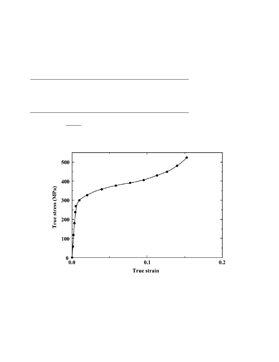
Excerpts from this work may be reproduced by instructors for distribution on a not-for-profit basis for testing or instructional purposes only to
students enrolled in courses for which the textbook has been adopted. Any other reproduction or translation of this work beyond that permitted
by Sections 107 or 108 of the 1976 United States Copyright Act without the permission of the copyright owner is unlawful.
6.41 Using the data in Problem 6.28 and Equations 6.15, 6.16, and 6.18a, generate a true stress–true
strain plot for aluminum. Equation 6.18a becomes invalid past the point at which necking begins; therefore,
measured diameters are given below for the last four data points, which should be used in true stress computations.
Load
Length
Diameter
N
lb
f
mm
in.
mm
in.
46,100
10,400
56.896
2.240
11.71
0.461
42,400
10,100
57.658
2.270
10.95
0.431
42,600
9,600
58.420
2.300
10.62
0.418
36,400
8,200
59.182
2.330
9.40
0.370
Solution
These true stress-strain data are plotted below.

Excerpts from this work may be reproduced by instructors for distribution on a not-for-profit basis for testing or instructional purposes only to
students enrolled in courses for which the textbook has been adopted. Any other reproduction or translation of this work beyond that permitted
by Sections 107 or 108 of the 1976 United States Copyright Act without the permission of the copyright owner is unlawful.
6.42 A tensile test is performed on a metal specimen, and it is found that a true plastic strain of 0.20 is
produced when a true stress of 575 MPa (83,500 psi) is applied; for the same metal, the value of K in Equation 6.19
is 860 MPa (125,000 psi). Calculate the true strain that results from the application of a true stress of 600 MPa
(87,000 psi).
Solution
It first becomes necessary to solve for n in Equation 6.19. Taking logarithms of this expression and after
rearrangement we have
n =
log
σ
T
− log K
log
ε
T
And, incorporating values of the parameters provided in the problem statement leads to
n =
log (575 MPa)
− log (860 MPa)
log (0.20)
= 0.250
Expressing
ε
T
as the dependent variable (Equation 6.19), and then solving for its value from the data stipulated in
the problem statement, leads to
ε
T
=
σ
T
K
1/n
=
600 MPa
860 MPa
1/0.250
= 0.237

Excerpts from this work may be reproduced by instructors for distribution on a not-for-profit basis for testing or instructional purposes only to
students enrolled in courses for which the textbook has been adopted. Any other reproduction or translation of this work beyond that permitted
by Sections 107 or 108 of the 1976 United States Copyright Act without the permission of the copyright owner is unlawful.
6.43 For some metal alloy, a true stress of 415 MPa (60,175 psi) produces a plastic true strain of 0.475.
How much will a specimen of this material elongate when a true stress of 325 MPa (46,125 psi) is applied if the
original length is 300 mm (11.8 in.)? Assume a value of 0.25 for the strain-hardening exponent n.
Solution
Solution of this problem requires that we utilize Equation 6.19. It is first necessary to solve for K from the
given true stress and strain. Rearrangement of this equation yields
K =
σ
T
(
ε
T
)
n
=
415 MPa
(0.475)
0.25
= 500 MPa (72, 500 psi)
Next we must solve for the true strain produced when a true stress of 325 MPa is applied, also using Equation 6.19.
Thus
ε
T
=
σ
T
K
1/n
=
325 MPa
500 MPa
1/0.25
= 0.179 = ln
l
i
l
0
Now, solving for l
i
gives
l
i
= l
0
e
0.179
= (300 mm) e
0.179
= 358.8 mm (14.11 in.)
And finally, the elongation ∆l is just
∆l = l
i
− l
0
= 358.8 mm
− 300 mm = 58.8 mm (2.31 in.)

Excerpts from this work may be reproduced by instructors for distribution on a not-for-profit basis for testing or instructional purposes only to
students enrolled in courses for which the textbook has been adopted. Any other reproduction or translation of this work beyond that permitted
by Sections 107 or 108 of the 1976 United States Copyright Act without the permission of the copyright owner is unlawful.
6.44 The following true stresses produce the corresponding true plastic strains for a brass alloy:
True Stress (psi)
True Strain
50,000
0.10
60,000
0.20
What true stress is necessary to produce a true plastic strain of 0.25?
Solution
For this problem, we are given two values of
ε
T
and
σ
T
,
from which we are asked to calculate the true
stress which produces a true plastic strain of 0.25. Employing Equation 6.19, we may set up two simultaneous
equations with two unknowns (the unknowns being K and n), as
log (50, 000 psi) = log K + n log (0.10)
log (60, 000 psi) = log K + n log (0.20)
Solving for n from these two expressions yields
n =
log (50, 000)
− log (60,000)
log (0.10 )
− log (0.20)
= 0.263
and for K
log K = 4.96 or K = 10
4.96
= 91,623 psi
Thus, for
ε
T
= 0.25
σ
T
= K (
ε
T
)
n
= (91, 623 psi)(0.25)
0.263
= 63, 700 psi (440 MPa)

Excerpts from this work may be reproduced by instructors for distribution on a not-for-profit basis for testing or instructional purposes only to
students enrolled in courses for which the textbook has been adopted. Any other reproduction or translation of this work beyond that permitted
by Sections 107 or 108 of the 1976 United States Copyright Act without the permission of the copyright owner is unlawful.
6.45 For a brass alloy, the following engineering stresses produce the corresponding plastic engineering
strains, prior to necking:
Engineering Stress (MPa)
Engineering Strain
235
0.194
250
0.296
On the basis of this information, compute the engineering stress necessary to produce an engineering strain of 0.25.
Solution
For this problem we first need to convert engineering stresses and strains to true stresses and strains so that
the constants K and n in Equation 6.19 may be determined. Since
σ
T
=
σ(1 + ε) then
σ
T 1
= (235 MPa)(1 + 0.194) = 280 MPa
σ
T 2
= (250 MPa)(1 + 0.296) = 324 MPa
Similarly for strains, since
ε
T
= ln(1 +
ε) then
ε
T 1
= ln (1 + 0.194) = 0.177
ε
T 2
= ln (1 + 0.296) = 0.259
Taking logarithms of Equation 6.19, we get
log
σ
T
= log K + n log
ε
T
which allows us to set up two simultaneous equations for the above pairs of true stresses and true strains, with K and
n as unknowns. Thus
log (280) = log K + n log (0.177)
log (324) = log K + n log (0.259)
Solving for these two expressions yields K = 543 MPa and n = 0.383.

Excerpts from this work may be reproduced by instructors for distribution on a not-for-profit basis for testing or instructional purposes only to
students enrolled in courses for which the textbook has been adopted. Any other reproduction or translation of this work beyond that permitted
by Sections 107 or 108 of the 1976 United States Copyright Act without the permission of the copyright owner is unlawful.
Now, converting
ε = 0.25 to true strain
ε
T
= ln (1 + 0.25) = 0.223
The corresponding
σ
T
to give this value of
ε
T
(using Equation 6.19) is just
σ
T
= K
ε
T
n
= (543 MPa)(0.223)
0.383
= 306 MPa
Now converting this value of
σ
T
to an engineering stress using Equation 6.18a gives
σ =
σ
T
1
+ ε
=
306 MPa
1
+ 0.25
= 245 MPa

Excerpts from this work may be reproduced by instructors for distribution on a not-for-profit basis for testing or instructional purposes only to
students enrolled in courses for which the textbook has been adopted. Any other reproduction or translation of this work beyond that permitted
by Sections 107 or 108 of the 1976 United States Copyright Act without the permission of the copyright owner is unlawful.
6.46 Find the toughness (or energy to cause fracture) for a metal that experiences both elastic and plastic
deformation. Assume Equation 6.5 for elastic deformation, that the modulus of elasticity is 172 GPa (25
× 10
6
psi),
and that elastic deformation terminates at a strain of 0.01. For plastic deformation, assume that the relationship
between stress and strain is described by Equation 6.19, in which the values for K and n are 6900 MPa (1
× 10
6
psi)
and 0.30, respectively. Furthermore, plastic deformation occurs between strain values of 0.01 and 0.75, at which
point fracture occurs.
Solution
This problem calls for us to compute the toughness (or energy to cause fracture). The easiest way to do
this is to integrate both elastic and plastic regions, and then add them together.
Toughness =
σ dε
∫
=
E
εd ε
0
0.01
∫
+
K
ε
n
d
ε
0.01
0.75
∫
=
E
ε
2
2
0
0.01
+
K
(n
+ 1)
ε
(n
+1)
0.01
0.75
=
172
× 10
9
N/m
2
2
(0.01)
2
+
6900
× 10
6
N/ m
2
(1.0
+ 0.3)
(0.75)
1.3
− (0.01)
1.3
[
]
= 3.65
× 10
9
J/m
3
(
5.29
× 10
5
in.-lb
f
/in.
3
)

Excerpts from this work may be reproduced by instructors for distribution on a not-for-profit basis for testing or instructional purposes only to
students enrolled in courses for which the textbook has been adopted. Any other reproduction or translation of this work beyond that permitted
by Sections 107 or 108 of the 1976 United States Copyright Act without the permission of the copyright owner is unlawful.
6.47 For a tensile test, it can be demonstrated that necking begins when
d
σ
T
d
ε
T
= σ
T
(6.26)
Using Equation 6.19, determine the value of the true strain at this onset of necking.
Solution
Let us take the derivative of Equation 6.19, set it equal to
σ
T
, and then solve for
ε
T
from the resulting
expression. Thus
d K (
ε
T )
n
[
]
d
ε
T
= Kn (
ε
T )
( n
−1)
=
σ
T
However, from Equation 6.19,
σ
T
= K(
ε
T
)
n
, which, when substituted into the above expression, yields
Kn (
ε
T
)
( n - 1)
= K (
ε
T
)
n
Now solving for
ε
T
from this equation leads to
ε
T
= n
as the value of the true strain at the onset of necking.
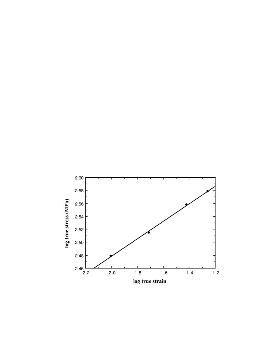
Excerpts from this work may be reproduced by instructors for distribution on a not-for-profit basis for testing or instructional purposes only to
students enrolled in courses for which the textbook has been adopted. Any other reproduction or translation of this work beyond that permitted
by Sections 107 or 108 of the 1976 United States Copyright Act without the permission of the copyright owner is unlawful.
6.48 Taking the logarithm of both sides of Equation 6.19 yields
log σ
T
= log K + n log
∈
T
(6.27)
Thus, a plot of log σ
T
versus log
∈
T
in the plastic region to the point of necking should yield a straight line having
a slope of n and an interc
ept (at log σ
T
= 0) of log K.
Using the appropriate data tabulated in Problem 6.29, make a plot of log σ
T
versus log
∈
T
and determine
the values of n and K. It will be necessary to convert engineering stresses and strains to true stresses and strains
using Equations 6.18a and 6.18b.
Solution
This problem calls for us to utilize the appropriate data from Problem 6.29 in order to determine the values
of n and K for this material. From Equation 6.27 the slope and intercept of a log
σ
T
versus log
ε
T
plot will yield n
and log K, respectively. However, Equation 6.19 is only valid in the region of plastic deformation to the point of
necking; thus, only the 7th, 8th, 9th, and 10th data points may be utilized. The log-log plot with these data points is
given below.
The slope yields a value of 0.136 for n, whereas the intercept gives a value of 2.7497 for log K, and thus K =
10
2.7497
= 562 MPa.

Excerpts from this work may be reproduced by instructors for distribution on a not-for-profit basis for testing or instructional purposes only to
students enrolled in courses for which the textbook has been adopted. Any other reproduction or translation of this work beyond that permitted
by Sections 107 or 108 of the 1976 United States Copyright Act without the permission of the copyright owner is unlawful.
Elastic Recovery After Plastic Deformation
6.49 A cylindrical specimen of a brass alloy 7.5 mm (0.30 in.) in diameter and 90.0 mm (3.54 in.) long is
pulled in tension with a force of 6000 N (1350 lb
f
); the force is subsequently released.
(a) Compute the final length of the specimen at this time. The tensile stress–strain behavior for this alloy is
shown in Figure 6.12.
(b) Compute the final specimen length when the load is increased to 16,500 N (3700 lb
f
) and then released.
Solution
(a) In order to determine the final length of the brass specimen when the load is released, it first becomes
necessary to compute the applied stress using Equation 6.1; thus
σ =
F
A
0
=
F
π
d
0
2
2
=
6000 N
π
7.5
× 10
−3
m
2
2
= 136 MPa (19, 000 psi)
Upon locating this point on the stress-strain curve (Figure 6.12), we note that it is in the linear, elastic region;
therefore, when the load is released the specimen will return to its original length of 90 mm (3.54 in.).
(b) In this portion of the problem we are asked to calculate the final length, after load release, when the
load is increased to 16,500 N (3700 lb
f
). Again, computing the stress
σ =
16, 500 N
π
7.5
× 10
−3
m
2
2
= 373 MPa (52, 300 psi)
The point on the stress-strain curve corresponding to this stress is in the plastic region. We are able to estimate the
amount of permanent strain by drawing a straight line parallel to the linear elastic region; this line intersects the
strain axis at a strain of about 0.08 which is the amount of plastic strain. The final specimen length l
i
may be
determined from a rearranged form of Equation 6.2 as
l
i
= l
0
(1 +
ε) = (90 mm)(1 + 0.08) = 97.20 mm (3.82 in.)

Excerpts from this work may be reproduced by instructors for distribution on a not-for-profit basis for testing or instructional purposes only to
students enrolled in courses for which the textbook has been adopted. Any other reproduction or translation of this work beyond that permitted
by Sections 107 or 108 of the 1976 United States Copyright Act without the permission of the copyright owner is unlawful.
6.50 A steel alloy specimen having a rectangular cross section of dimensions 12.7 mm × 6.4 mm (0.5 in. ×
0.25 in.) has the stress–strain behavior shown in Figure 6.21. If this specimen is subjected to a tensile force of
38,000 N (8540 lb
f
) then
(a) Determine the elastic and plastic strain values.
(b) If its original length is 460 mm (18.0 in.), what will be its final length after the load in part (a) is
applied and then released?
Solution
(a) We are asked to determine both the elastic and plastic strain values when a tensile force of 38,000 N
(8540 lb
f
) is applied to the steel specimen and then released. First it becomes necessary to determine the applied
stress using Equation 6.1; thus
σ =
F
A
0
=
F
b
0
d
0
where b
0
and d
0
are cross-sectional width and depth (12.7 mm and 6.4 mm, respectively). Thus
σ =
38, 000 N
(
12.7
× 10
−3
m
)(
6.4
× 10
−3
m
)
= 468
× 10
6
N / m
2
= 468 MPa (68,300 psi)
From Figure 6.21, this point is in the plastic region so the specimen will be both elastic and plastic strains. The total
strain at this point,
ε
t
, is about 0.010. We are able to estimate the amount of permanent strain recovery
ε
e
from
Hooke's law, Equation 6.5 as
ε
e
=
σ
E
And, since E = 207 GPa for steel (Table 6.1)
ε
e
=
468 MPa
207
× 10
3
MPa
= 0.00226
The value of the plastic strain,
ε
p
is just the difference between the total and elastic strains; that is
ε
p
=
ε
t
–
ε
e
= 0.010 – 0.00226 = 0.00774

Excerpts from this work may be reproduced by instructors for distribution on a not-for-profit basis for testing or instructional purposes only to
students enrolled in courses for which the textbook has been adopted. Any other reproduction or translation of this work beyond that permitted
by Sections 107 or 108 of the 1976 United States Copyright Act without the permission of the copyright owner is unlawful.
(b) If the initial length is 460 mm (18.0 in.) then the final specimen length l
i
may be determined from a
rearranged form of Equation 6.2 using the plastic strain value as
l
i
= l
0
(
1 +
ε
p
)
= (460 mm)(1 + 0.00774) = 463.6 mm (18.14 in.)
Excerpts from this work may be reproduced by instructors for distribution on a not-for-profit basis for testing or instructional purposes only to
students enrolled in courses for which the textbook has been adopted. Any other reproduction or translation of this work beyond that permitted
by Sections 107 or 108 of the 1976 United States Copyright Act without the permission of the copyright owner is unlawful.
Hardness
6.51 (a) A 10-mm-diameter Brinell hardness indenter produced an indentation 1.62 mm in diameter in a
steel alloy when a load of 500 kg was used. Compute the HB of this material.
(b) What will be the diameter of an indentation to yield a hardness of 450 HB when a 500 kg load is used?
Solution
(a) We are asked to compute the Brinell hardness for the given indentation. It is necessary to use the
equation in Table 6.5 for HB, where P = 500 kg, d = 1.62 mm, and D = 10 mm. Thus, the Brinell hardness is
computed as
HB =
2P
π D D − D
2
− d
2
[
]
=
(2)(500 kg)
(
π)(10 mm) 10 mm − (10 mm)
2
− (1.62 mm)
2
[
]
= 241
(b) This part of the problem calls for us to determine the indentation diameter d which will yield a 450 HB
when P = 500 kg. Solving for d from the equation in Table 6.5 gives
d =
D
2
− D −
2P
(HB)
π D
2
=
(10mm)
2
− 10 mm −
(2)(500 kg)
(450)(
π)(10 mm)
2
= 1.19 mm

Excerpts from this work may be reproduced by instructors for distribution on a not-for-profit basis for testing or instructional purposes only to
students enrolled in courses for which the textbook has been adopted. Any other reproduction or translation of this work beyond that permitted
by Sections 107 or 108 of the 1976 United States Copyright Act without the permission of the copyright owner is unlawful.
6.52 Estimate the Brinell and Rockwell hardnesses for the following:
(a) The naval brass for which the stress–strain behavior is shown in Figure 6.12.
(b) The steel alloy for which the stress–strain behavior is shown in Figure 6.21.
Solution
This problem calls for estimations of Brinell and Rockwell hardnesses.
(a) For the brass specimen, the stress-strain behavior for which is shown in Figure 6.12, the tensile
strength is 450 MPa (65,000 psi). From Figure 6.19, the hardness for brass corresponding to this tensile strength is
about 125 HB or 70 HRB.
(b) The steel alloy (Figure 6.21) has a tensile strength of about 515 MPa (74,700 psi) [Problem 6.25(d)].
This corresponds to a hardness of about 160 HB or ~90 HRB from the line for steels in Figure 6.19. Alternately,
using Equation 6.20a
HB
=
TS(MPa)
3.45
=
515 MPa
3.45
= 149

Excerpts from this work may be reproduced by instructors for distribution on a not-for-profit basis for testing or instructional purposes only to
students enrolled in courses for which the textbook has been adopted. Any other reproduction or translation of this work beyond that permitted
by Sections 107 or 108 of the 1976 United States Copyright Act without the permission of the copyright owner is unlawful.
6.53 Using the data represented in Figure 6.19, specify equations relating tensile strength and Brinell
hardness for brass and nodular cast iron, similar to Equations 6.20a and 6.20b for steels.
Solution
These equations, for a straight line, are of the form
TS = C + (E)(HB)
where TS is the tensile strength, HB is the Brinell hardness, and C and E are constants, which need to be
determined.
One way to solve for C and E is analytically--establishing two equations using TS and HB data points on
the plot, as
(TS)
1
= C + (E)(BH)
1
(TS)
2
= C + (E)(BH)
2
Solving for E from these two expressions yields
E =
(TS)
1
− (TS)
2
(HB)
2
− (HB)
1
For nodular cast iron, if we make the arbitrary choice of (HB)
1
and (HB)
2
as 200 and 300, respectively, then, from
Figure 6.19, (TS)
1
and (TS)
2
take on values of 600 MPa (87,000 psi) and 1100 MPa (160,000 psi), respectively.
Substituting these values into the above expression and solving for E gives
E =
600 MPa
− 1100 MPa
200 HB
− 300 HB
= 5.0 MPa/HB (730 psi/HB)
Now, solving for C yields
C = (TS)
1
– (E)(BH)
1
= 600 MPa - (5.0 MPa/HB)(200 HB) = – 400 MPa (– 59,000 psi)
Thus, for nodular cast iron, these two equations take the form

Excerpts from this work may be reproduced by instructors for distribution on a not-for-profit basis for testing or instructional purposes only to
students enrolled in courses for which the textbook has been adopted. Any other reproduction or translation of this work beyond that permitted
by Sections 107 or 108 of the 1976 United States Copyright Act without the permission of the copyright owner is unlawful.
TS(MPa) = – 400 + 5.0 x HB
TS(psi) = – 59,000 + 730 x HB
Now for brass, we take (HB)
1
and (HB)
2
as 100 and 200, respectively, then, from Figure 7.31, (TS)
1
and
(TS)
2
take on values of 370 MPa (54,000 psi) and 660 MPa (95,000 psi), respectively. Substituting these values
into the above expression and solving for E gives
E =
370 MPa
− 660 MPa
100 HB
− 200 HB
= 2.9 MPa/HB (410 psi/HB)
Now, solving for C yields
C = (TS)
1
– (E)(BH)
1
= 370 MPa – (2.9 MPa/HB)(100 HB) = 80 MPa (13,000 psi)
Thus, for brass these two equations take the form
TS(MPa) = 80 + 2.9 x HB
TS(psi) = 13,000 + 410 x HB

Excerpts from this work may be reproduced by instructors for distribution on a not-for-profit basis for testing or instructional purposes only to
students enrolled in courses for which the textbook has been adopted. Any other reproduction or translation of this work beyond that permitted
by Sections 107 or 108 of the 1976 United States Copyright Act without the permission of the copyright owner is unlawful.
Variability of Material Properties
6.54 Cite five factors that lead to scatter in measured material properties.
Solution
The five factors that lead to scatter in measured material properties are the following: (1) test method; (2)
variation in specimen fabrication procedure; (3) operator bias; (4) apparatus calibration; and (5) material
inhomogeneities and/or compositional differences.
Excerpts from this work may be reproduced by instructors for distribution on a not-for-profit basis for testing or instructional purposes only to
students enrolled in courses for which the textbook has been adopted. Any other reproduction or translation of this work beyond that permitted
by Sections 107 or 108 of the 1976 United States Copyright Act without the permission of the copyright owner is unlawful.
6.55 Below are tabulated a number of Rockwell B hardness values that were measured on a single steel
specimen. Compute average and standard deviation hardness values.
83.3
80.7
86.4
88.3
84.7
85.2
82.8
87.8
86.9
86.2
83.5
84.4
87.2
85.5
86.3
Solution
The average of the given hardness values is calculated using Equation 6.21 as
HRB =
HRB
i
i
=1
15
∑
15
=
83.3
+ 88.3 + 82.8 . . . . + 86.3
15
= 85.3
And we compute the standard deviation using Equation 6.22 as follows:
s =
HRB
i
− HRB
(
)
2
i
=1
15
∑
15
− 1
=
(
83.3
− 85.3)
2
+ (88.3 − 85.3)
2
+ . . . . + (86.3 − 85.3)
2
14
1/2
=
60.31
14
= 2.08

Excerpts from this work may be reproduced by instructors for distribution on a not-for-profit basis for testing or instructional purposes only to
students enrolled in courses for which the textbook has been adopted. Any other reproduction or translation of this work beyond that permitted
by Sections 107 or 108 of the 1976 United States Copyright Act without the permission of the copyright owner is unlawful.
Design/Safety Factors
6.56 Upon what three criteria are factors of safety based?
Solution
The criteria upon which factors of safety are based are (1) consequences of failure, (2) previous
experience, (3) accuracy of measurement of mechanical forces and/or material properties, and (4) economics.

Excerpts from this work may be reproduced by instructors for distribution on a not-for-profit basis for testing or instructional purposes only to
students enrolled in courses for which the textbook has been adopted. Any other reproduction or translation of this work beyond that permitted
by Sections 107 or 108 of the 1976 United States Copyright Act without the permission of the copyright owner is unlawful.
6.57 Determine working stresses for the two alloys that have the stress–strain behaviors shown in Figures
6.12 and 6.21.
Solution
The working stresses for the two alloys the stress-strain behaviors of which are shown in Figures 6.12 and
6.21 are calculated by dividing the yield strength by a factor of safety, which we will take to be 2. For the brass
alloy (Figure 6.12), since
σ
y
= 250 MPa (36,000 psi), the working stress is 125 MPa (18,000 psi), whereas for the
steel alloy (Figure 6.21),
σ
y
= 400 MPa (58,000 psi), and, therefore,
σ
w
= 200 MPa (29,000 psi).
Excerpts from this work may be reproduced by instructors for distribution on a not-for-profit basis for testing or instructional purposes only to
students enrolled in courses for which the textbook has been adopted. Any other reproduction or translation of this work beyond that permitted
by Sections 107 or 108 of the 1976 United States Copyright Act without the permission of the copyright owner is unlawful.
DESIGN PROBLEMS
6.D1 A large tower is to be supported by a series of steel wires. It is estimated that the load on each wire
will be 11,100 N (2500 lb
f
). Determine the minimum required wire diameter assuming a factor of safety of 2 and a
yield strength of 1030 MPa (150,000 psi).
Solution
For this problem the working stress is computed using Equation 6.24 with N = 2, as
σ
w
=
σ
y
2
=
1030 MPa
2
= 515 MPa (75, 000 psi )
Since the force is given, the area may be determined from Equation 6.1, and subsequently the original diameter d
0
may be calculated as
A
0
=
F
σ
w
=
π
d
0
2
2
And
d
0
=
4F
π σ
w
=
(4)(11,100 N)
π
(
515
× 10
6
N / m
2
)
= 5.23
× 10
-3
m = 5.23 mm (0.206 in.)

Excerpts from this work may be reproduced by instructors for distribution on a not-for-profit basis for testing or instructional purposes only to
students enrolled in courses for which the textbook has been adopted. Any other reproduction or translation of this work beyond that permitted
by Sections 107 or 108 of the 1976 United States Copyright Act without the permission of the copyright owner is unlawful.
6.D2 (a) Gaseous hydrogen at a constant pressure of 1.013 MPa (10 atm) is to flow within the inside of a
thin-walled cylindrical tube of nickel that has a radius of 0.1 m. The temperature of the tube is to be 300
°C and the
pressure of hydrogen outside of the tube will be maintained at 0.01013 MPa (0.1 atm). Calculate the minimum wall
thickness if the diffusion flux is to be no greater than 1
× 10
-7
mol/m
2
-s. The concentration of hydrogen in the
nickel, C
H
(in moles hydrogen per m
3
of Ni) is a function of hydrogen pressure, P
H
2
(in MPa) and absolute
temperature (T) according to
C
H
= 30.8 p
H
2
exp
−
12.3 kJ/mol
RT
(6.28)
Furthermore, the diffusion coefficient for the diffusion of H in Ni depends on temperature as
D
H
= 4.76 × 10
−7
exp
−
39.56 kJ/mol
RT
(6.29)
(b) For thin-walled cylindrical tubes that are pressurized, the circumferential stress is a function of the
pressure difference across the wall (Δp), cylinder radius (r), and tube thickness (Δx) as
σ =
r
∆p
4
∆x
(6.30)
Compute the circumferential stress to which the walls of this pressurized cylinder are exposed.
(c) The room-temperature yield strength of Ni is 100 MPa (15,000 psi) and, furthermore,
σ
y
diminishes
about 5 MPa for every 50
°C rise in temperature. Would you expect the wall thickness computed in part (b) to be
suitable for this Ni cylinder at 300
°C? Why or why not?
(d) If this thickness is found to be suitable, compute the minimum thickness that could be used without any
deformation of the tube walls. How much would the diffusion flux increase with this reduction in thickness? On the
other hand, if the thickness determined in part (c) is found to be unsuitable, then specify a minimum thickness that
you would use. In this case, how much of a diminishment in diffusion flux would result?
Solution
(a) This portion of the problem asks for us to compute the wall thickness of a thin-walled cylindrical Ni
tube at 300
°C through which hydrogen gas diffuses. The inside and outside pressures are, respectively, 1.1013 and
0.01013 MPa, and the diffusion flux is to be no greater than 1
× 10
-7
mol/m
2
-s. This is a steady-state diffusion
problem, which necessitates that we employ Equation 5.3. The concentrations at the inside and outside wall faces
may be determined using Equation 6.28, and, furthermore, the diffusion coefficient is computed using Equation
6.29. Solving for
∆x (using Equation 5.3)
∆x = −
D
∆C
J
Excerpts from this work may be reproduced by instructors for distribution on a not-for-profit basis for testing or instructional purposes only to
students enrolled in courses for which the textbook has been adopted. Any other reproduction or translation of this work beyond that permitted
by Sections 107 or 108 of the 1976 United States Copyright Act without the permission of the copyright owner is unlawful.
=
−
1
1
× 10
−7
mol/m
2
− s
×
(
4.76
× 10
-7
)
exp
−
39, 560 J / mol
(8.31 J/mol - K)(300
+ 273 K)
×
(30.8) exp
−
12, 300 J/mol
(8.31 J/mol - K)(300
+ 273 K)
0.01013 MPa − 1.1013 MPa
(
)
= 0.0025 m = 2.5 mm
(b) Now we are asked to determine the circumferential stress:
σ =
r
∆p
4
∆x
=
(0.10 m)(1.013 MPa
− 0.01013 MPa)
(4)(0.0025 m)
= 10.0 MPa
(c) Now we are to compare this value of stress to the yield strength of Ni at 300
°C, from which it is
possible to determine whether or not the 2.5 mm wall thickness is suitable. From the information given in the
problem, we may write an equation for the dependence of yield strength (
σ
y
) on temperature (T) as follows:
σ
y
= 100 MPa
−
5 MPa
50
°C
T
− T
r
(
)
where T
r
is room temperature and for temperature in degrees Celsius. Thus, at 300
°C
σ
y
= 100 MPa
− (0.1 MPa/°C) (300°C − 20°C) = 72 MPa
Inasmuch as the circumferential stress (10 MPa) is much less than the yield strength (72 MPa), this thickness is
entirely suitable.
Excerpts from this work may be reproduced by instructors for distribution on a not-for-profit basis for testing or instructional purposes only to
students enrolled in courses for which the textbook has been adopted. Any other reproduction or translation of this work beyond that permitted
by Sections 107 or 108 of the 1976 United States Copyright Act without the permission of the copyright owner is unlawful.
(d) And, finally, this part of the problem asks that we specify how much this thickness may be reduced and
still retain a safe design. Let us use a working stress by dividing the yield stress by a factor of safety, according to
Equation 6.24. On the basis of our experience, let us use a value of 2.0 for N. Thus
σ
w
=
σ
y
N
=
72 MPa
2
= 36 MPa
Using this value for
σ
w
and Equation 6.30, we now compute the tube thickness as
∆x =
r
∆p
4
σ
w
=
(0.10 m)(1.013 MPa
− 0.01013 MPa)
4(36 MPa)
= 0.00070 m = 0.70 mm
Substitution of this value into Fick's first law we calculate the diffusion flux as follows:
J =
− D
∆C
∆x
=
−
(
4.76
× 10
-7
)
exp
−
39, 560 J/mol
(8.31 J/mol - K)(300
+ 273 K)
×
(30.8) exp
−
12, 300 J / mol
(8.31 J/mol - K)(300
+ 273 K)
0.01013 MPa − 1.013 MPa
(
)
0.0007 m
= 3.53
× 10
-7
mol/m
2
-s
Thus, the flux increases by approximately a factor of 3.5, from 1
× 10
-7
to 3.53
× 10
-7
mol/m
2
-s with this reduction
in thickness.
Excerpts from this work may be reproduced by instructors for distribution on a not-for-profit basis for testing or instructional purposes only to
students enrolled in courses for which the textbook has been adopted. Any other reproduction or translation of this work beyond that permitted
by Sections 107 or 108 of the 1976 United States Copyright Act without the permission of the copyright owner is unlawful.
6.D3 Consider the steady-state diffusion of hydrogen through the walls of a cylindrical nickel tube as
described in Problem 6.D2. One design calls for a diffusion flux of 5
× 10
-8
mol/m
2
-s, a tube radius of 0.125 m, and
inside and outside pressures of 2.026 MPa (20 atm) and 0.0203 MPa (0.2 atm), respectively; the maximum
allowable temperature is 450
°C. Specify a suitable temperature and wall thickness to give this diffusion flux and
yet ensure that the tube walls will not experience any permanent deformation.
Solution
This problem calls for the specification of a temperature and cylindrical tube wall thickness that will give a
diffusion flux of 5
× 10
-8
mol/m
2
-s for the diffusion of hydrogen in nickel; the tube radius is 0.125 m and the
inside and outside pressures are 2.026 and 0.0203 MPa, respectively. There are probably several different
approaches that may be used; and, of course, there is not one unique solution. Let us employ the following
procedure to solve this problem: (1) assume some wall thickness, and, then, using Fick's first law for diffusion
(which also employs Equations 5.3 and 6.29), compute the temperature at which the diffusion flux is that required;
(2) compute the yield strength of the nickel at this temperature using the dependence of yield strength on
temperature as stated in Problem 6.D2; (3) calculate the circumferential stress on the tube walls using Equation
6.30; and (4) compare the yield strength and circumferential stress values--the yield strength should probably be at
least twice the stress in order to make certain that no permanent deformation occurs. If this condition is not met
then another iteration of the procedure should be conducted with a more educated choice of wall thickness.
As a starting point, let us arbitrarily choose a wall thickness of 2 mm (2
× 10
-3
m). The steady-state
diffusion equation, Equation 5.3, takes the form
J =
− D
∆C
∆x
= 5
× 10
-8
mol/m
2
-s
=
−
(
4.76
× 10
-7
)
exp
−
39, 560 J/mol
(8.31 J/mol - K)(T)
×
(30.8) exp
−
12, 300 J/mol
(8.31 J/mol - K)(T)
0.0203 MPa − 2.026 MPa
(
)
0.002 m
Solving this expression for the temperature T gives T = 514 K = 241
°C; this value is satisfactory inasmuch as it is
less than the maximum allowable value (450
°C).
The next step is to compute the stress on the wall using Equation 6.30; thus

Excerpts from this work may be reproduced by instructors for distribution on a not-for-profit basis for testing or instructional purposes only to
students enrolled in courses for which the textbook has been adopted. Any other reproduction or translation of this work beyond that permitted
by Sections 107 or 108 of the 1976 United States Copyright Act without the permission of the copyright owner is unlawful.
σ =
r
∆p
4
∆x
=
(0.125 m)(2.026 MPa
− 0.0203 MPa)
(4)
(
2
× 10
−3
m
)
= 31.3 MPa
Now, the yield strength (
σ
y
) of Ni at this temperature may be computed using the expression
σ
y
= 100 MPa
−
5 MPa
50
°C
T
− T
r
(
)
where T
r
is room temperature. Thus,
σ
y
= 100 MPa – (0.1 MPa/
°C)(241°C – 20°C) = 77.9 MPa
Inasmuch as this yield strength is greater than twice the circumferential stress, wall thickness and temperature
values of 2 mm and 241
°C are satisfactory design parameters.

Excerpts from this work may be reproduced by instructors for distribution on a not-for-profit basis for testing or instructional purposes only to
students enrolled in courses for which the textbook has been adopted. Any other reproduction or translation of this work beyond that permitted
by Sections 107 or 108 of the 1976 United States Copyright Act without the permission of the copyright owner is unlawful.
CHAPTER 7
DISLOCATIONS AND STRENGTHENING MECHANISMS
PROBLEM SOLUTIONS
Basic Concepts of Dislocations
Characteristics of Dislocations
7.1 To provide some perspective on the dimensions of atomic defects, consider a metal specimen that has a
dislocation density of 10
4
mm
-2
. Suppose that all the dislocations in 1000 mm
3
(1 cm
3
) were somehow removed and
linked end to end. How far (in miles) would this chain extend? Now suppose that the density is increased to 10
10
mm
-2
by cold working. What would be the chain length of dislocations in 1000 mm
3
of material?
Solution
The dislocation density is just the total dislocation length per unit volume of material (in this case per cubic
millimeters). Thus, the total length in 1000 mm
3
of material having a density of 10
4
mm
-2
is just
(
10
4
mm
-2
)(
1000 mm
3
)
= 10
7
mm = 10
4
m = 6.2 mi
Similarly, for a dislocation density of 10
10
mm
-2
, the total length is
(
10
10
mm
-2
)(
1000 mm
3
)
= 10
13
mm = 10
10
m = 6.2
× 10
6
mi
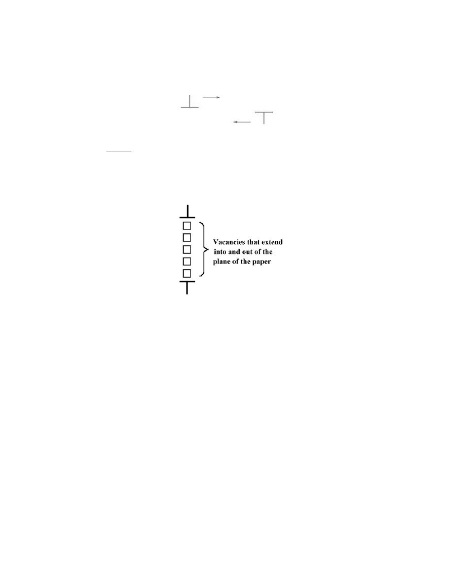
Excerpts from this work may be reproduced by instructors for distribution on a not-for-profit basis for testing or instructional purposes only to
students enrolled in courses for which the textbook has been adopted. Any other reproduction or translation of this work beyond that permitted
by Sections 107 or 108 of the 1976 United States Copyright Act without the permission of the copyright owner is unlawful.
7.2 Consider two edge dislocations of opposite sign and having slip planes that are separated by several
atomic distances as indicated in the diagram. Briefly describe the defect that results when these two dislocations
become aligned with each other.
Solution
When the two edge dislocations become aligned, a planar region of vacancies will exist between the
dislocations as:
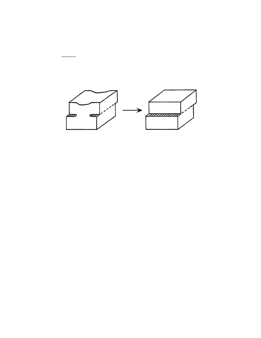
Excerpts from this work may be reproduced by instructors for distribution on a not-for-profit basis for testing or instructional purposes only to
students enrolled in courses for which the textbook has been adopted. Any other reproduction or translation of this work beyond that permitted
by Sections 107 or 108 of the 1976 United States Copyright Act without the permission of the copyright owner is unlawful.
7.3 Is it possible for two screw dislocations of opposite sign to annihilate each other? Explain your
answer.
Solution
It is possible for two screw dislocations of opposite sign to annihilate one another if their dislocation lines
are parallel. This is demonstrated in the figure below.

Excerpts from this work may be reproduced by instructors for distribution on a not-for-profit basis for testing or instructional purposes only to
students enrolled in courses for which the textbook has been adopted. Any other reproduction or translation of this work beyond that permitted
by Sections 107 or 108 of the 1976 United States Copyright Act without the permission of the copyright owner is unlawful.
7.4 For each of edge, screw, and mixed dislocations, cite the relationship between the direction of the
applied shear stress and the direction of dislocation line motion.
Solution
For the various dislocation types, the relationships between the direction of the applied shear stress and the
direction of dislocation line motion are as follows:
edge dislocation--parallel
screw dislocation--perpendicular
mixed dislocation--neither parallel nor perpendicular

Excerpts from this work may be reproduced by instructors for distribution on a not-for-profit basis for testing or instructional purposes only to
students enrolled in courses for which the textbook has been adopted. Any other reproduction or translation of this work beyond that permitted
by Sections 107 or 108 of the 1976 United States Copyright Act without the permission of the copyright owner is unlawful.
Slip Systems
7.5 (a) Define a slip system.
(b) Do all metals have the same slip system? Why or why not?
Solution
(a) A slip system is a crystallographic plane, and, within that plane, a direction along which dislocation
motion (or slip) occurs.
(b) All metals do not have the same slip system. The reason for this is that for most metals, the slip system
will consist of the most densely packed crystallographic plane, and within that plane the most closely packed
direction. This plane and direction will vary from crystal structure to crystal structure.
Excerpts from this work may be reproduced by instructors for distribution on a not-for-profit basis for testing or instructional purposes only to
students enrolled in courses for which the textbook has been adopted. Any other reproduction or translation of this work beyond that permitted
by Sections 107 or 108 of the 1976 United States Copyright Act without the permission of the copyright owner is unlawful.
7.6 (a) Compare planar densities (Section 3.11 and Problem 3.54) for the (100), (110), and (111) planes
for FCC.
(b) Compare planar densities (Problem 3.55) for the (100), (110), and (111) planes for BCC.
Solution
(a) For the FCC crystal structure, the planar density for the (110) plane is given in Equation 3.11 as
PD
110
(FCC)
=
1
4 R
2
2
=
0.177
R
2
Furthermore, the planar densities of the (100) and (111) planes are calculated in Homework Problem 3.54,
which are as follows:
PD
100
(FCC) =
1
4 R
2
=
0.25
R
2
PD
111
(FCC)
=
1
2 R
2
3
=
0.29
R
2
(b) For the BCC crystal structure, the planar densities of the (100) and (110) planes were determined in
Homework Problem 3.55, which are as follows:
PD
100
(BCC) =
3
16R
2
=
0.19
R
2
PD
110
(BCC)
=
3
8 R
2
2
=
0.27
R
2
Below is a BCC unit cell, within which is shown a (111) plane.
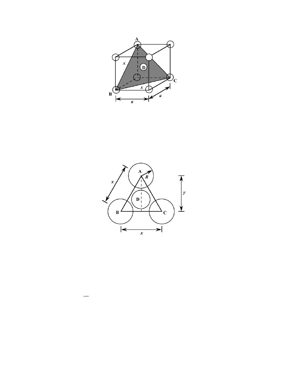
Excerpts from this work may be reproduced by instructors for distribution on a not-for-profit basis for testing or instructional purposes only to
students enrolled in courses for which the textbook has been adopted. Any other reproduction or translation of this work beyond that permitted
by Sections 107 or 108 of the 1976 United States Copyright Act without the permission of the copyright owner is unlawful.
(a)
The centers of the three corner atoms, denoted by A, B, and C lie on this plane. Furthermore, the (111) plane does
not pass through the center of atom D, which is located at the unit cell center. The atomic packing of this plane is
presented in the following figure; the corresponding atom positions from the Figure (a) are also noted.
(b)
Inasmuch as this plane does not pass through the center of atom D, it is not included in the atom count. One sixth of
each of the three atoms labeled A, B, and C is associated with this plane, which gives an equivalence of one-half
atom.
In Figure (b) the triangle with A, B, and C at its corners is an equilateral triangle. And, from Figure (b),
the area of this triangle is
xy
2
. The triangle edge length, x, is equal to the length of a face diagonal, as indicated in
Figure (a). And its length is related to the unit cell edge length, a, as
Excerpts from this work may be reproduced by instructors for distribution on a not-for-profit basis for testing or instructional purposes only to
students enrolled in courses for which the textbook has been adopted. Any other reproduction or translation of this work beyond that permitted
by Sections 107 or 108 of the 1976 United States Copyright Act without the permission of the copyright owner is unlawful.
x
2
= a
2
+ a
2
= 2a
2
or
x
= a 2
For BCC,
a
=
4 R
3
(Equation 3.3), and, therefore,
x
=
4R
2
3
Also, from Figure (b), with respect to the length y we may write
y
2
+
x
2
2
= x
2
which leads to
y
=
x
3
2
. And, substitution for the above expression for x yields
y
=
x
3
2
=
4 R 2
3
3
2
=
4 R
2
2
Thus, the area of this triangle is equal to
AREA
=
1
2
x y
=
1
2
4 R
2
3
4 R
2
2
=
8 R
2
3
And, finally, the planar density for this (111) plane is
PD
111
(BCC)
=
0.5 atom
8 R
2
3
=
3
16 R
2
=
0.11
R
2
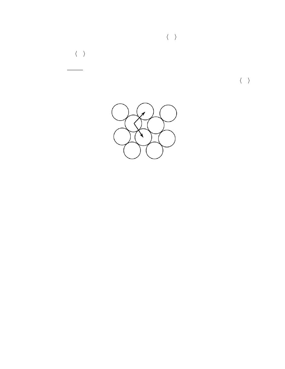
Excerpts from this work may be reproduced by instructors for distribution on a not-for-profit basis for testing or instructional purposes only to
students enrolled in courses for which the textbook has been adopted. Any other reproduction or translation of this work beyond that permitted
by Sections 107 or 108 of the 1976 United States Copyright Act without the permission of the copyright owner is unlawful.
7.7 One slip system for the BCC crystal structure is
110
{ }
111 . In a manner similar to Figure 7.6b,
sketch a
110
{ }
-type plane for the BCC structure, representing atom positions with circles. Now, using arrows,
indicate two different
111 slip directions within this plane.
Solution
Below is shown the atomic packing for a BCC
110
{ }
-type plane. The arrows indicate two different
111 -
type directions.
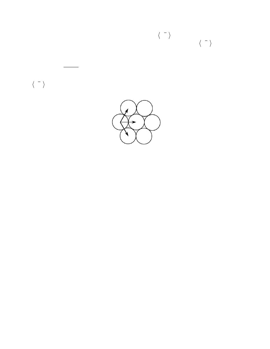
Excerpts from this work may be reproduced by instructors for distribution on a not-for-profit basis for testing or instructional purposes only to
students enrolled in courses for which the textbook has been adopted. Any other reproduction or translation of this work beyond that permitted
by Sections 107 or 108 of the 1976 United States Copyright Act without the permission of the copyright owner is unlawful.
7.8 One slip system for the HCP crystal structure is
0001
{
}
112 0 . In a manner similar to Figure 7.6b,
sketch a
0001
{
}
-type plane for the HCP structure and, using arrows, indicate three different
112 0 slip directions
within this plane. You might find Figure 3.8 helpful.
Solution
Below is shown the atomic packing for an HCP
0001
{
}
-type plane. The arrows indicate three different
112 0
-type directions.
Excerpts from this work may be reproduced by instructors for distribution on a not-for-profit basis for testing or instructional purposes only to
students enrolled in courses for which the textbook has been adopted. Any other reproduction or translation of this work beyond that permitted
by Sections 107 or 108 of the 1976 United States Copyright Act without the permission of the copyright owner is unlawful.
7.9 Equations 7.1a and 7.1b, expressions for Burgers vectors for FCC and BCC crystal structures, are of
the form
b
=
a
2
uvw
where a is the unit cell edge length. Also, since the magnitudes of these Burgers vectors may be determined from the
following equation:
b
=
a
2
u
2
+ v
2
+ w
2
(
)
1/2
(7.10)
determine values of |b| for aluminum and chromium. You may want to consult Table 3.1.
Solution
For Al, which has an FCC crystal structure, R = 0.1431 nm (Table 3.1) and a =
2 R 2
= 0.4047 nm
(Equation 3.1); also, from Equation 7.1a, the Burgers vector for FCC metals is
b
=
a
2
〈110〉
Therefore, the values for u, v, and w in Equation 7.10 are 1, 1, and 0, respectively. Hence, the magnitude of the
Burgers vector for Al is
b =
a
2
u
2
+ v
2
+ w
2
=
0.4047 nm
2
(1 )
2
+ (1 )
2
+ (0)
2
= 0.2862 nm
For Cr which has a BCC crystal structure, R = 0.1249 nm (Table 3.1) and
a
=
4 R
3
= 0.2884 nm (Equation
3.3); also, from Equation 7.1b, the Burgers vector for BCC metals is
b
=
a
2
〈111〉
Therefore, the values for u, v, and w in Equation 7.10 are 1, 1, and 1, respectively. Hence, the magnitude of the
Burgers vector for Cr is
b =
0.2884 nm
2
(1)
2
+ (1)
2
+ (1)
2
= 0.2498 nm
Excerpts from this work may be reproduced by instructors for distribution on a not-for-profit basis for testing or instructional purposes only to
students enrolled in courses for which the textbook has been adopted. Any other reproduction or translation of this work beyond that permitted
by Sections 107 or 108 of the 1976 United States Copyright Act without the permission of the copyright owner is unlawful.
7.10 (a) In the manner of Equations 7.1a, 7.1b, and 7.1c, specify the Burgers vector for the simple cubic
crystal structure. Its unit cell is shown in Figure 3.24. Also, simple cubic is the crystal structure for the edge
dislocation of Figure 4.3, and for its motion as presented in Figure 7.1. You may also want to consult the answer to
Concept Check 7.1.
(b) On the basis of Equation 7.10, formulate an expression for the magnitude of the Burgers vector, |b|, for
simple cubic.
Solution
(a) This part of the problem asks that we specify the Burgers vector for the simple cubic crystal structure
(and suggests that we consult the answer to Concept Check 7.1). This Concept Check asks that we select the slip
system for simple cubic from four possibilities. The correct answer is
100
{ }
010
. Thus, the Burgers vector will lie
in a
010
-type direction. Also, the unit slip distance is a (i.e., the unit cell edge length, Figures 4.3 and 7.1).
Therefore, the Burgers vector for simple cubic is
b = a 010
Or, equivalently
b = a 100
(b) The magnitude of the Burgers vector, |b|, for simple cubic is
b = a
(
1
2
+ 0
2
+ 0
2
)
1 / 2
=
a
Excerpts from this work may be reproduced by instructors for distribution on a not-for-profit basis for testing or instructional purposes only to
students enrolled in courses for which the textbook has been adopted. Any other reproduction or translation of this work beyond that permitted
by Sections 107 or 108 of the 1976 United States Copyright Act without the permission of the copyright owner is unlawful.
Slip in Single Crystals
7.11 Sometimes cos
φ cos λ in Equation 7.2 is termed the Schmid factor. Determine the magnitude of the
Schmid factor for an FCC single crystal oriented with its [100] direction parallel to the loading axis.
Solution
We are asked to compute the Schmid factor for an FCC crystal oriented with its [100] direction parallel to
the loading axis. With this scheme, slip may occur on the (111) plane and in the
[1 1 0] direction as noted in the
figure below.
The angle between the [100] and
[1 1 0] directions,
λ, may be determined using Equation 7.6
λ = cos
−1
u
1
u
2
+ v
1
v
2
+ w
1
w
2
u
1
2
+ v
1
2
+ w
1
2
(
)
u
2
2
+ v
2
2
+ w
2
2
(
)
where (for [100]) u
1
= 1
,
v
1
= 0, w
1
= 0, and (for
[1 1 0]
) u
2
= 1, v
2
= -1, w
2
= 0. Therefore,
λ is equal to
λ = cos
−1
(1)(1)
+ (0)(−1) + (0)(0)
(1)
2
+ (0)
2
+ (0)
2
[
]
(1)
2
+ (−1)
2
+ (0)
2
[
]
= cos
−1
1
2
= 45°
Excerpts from this work may be reproduced by instructors for distribution on a not-for-profit basis for testing or instructional purposes only to
students enrolled in courses for which the textbook has been adopted. Any other reproduction or translation of this work beyond that permitted
by Sections 107 or 108 of the 1976 United States Copyright Act without the permission of the copyright owner is unlawful.
Now, the angle
φ is equal to the angle between the normal to the (111) plane (which is the [111] direction), and the
[100] direction. Again from Equation 7.6, and for u
1
= 1
,
v
1
= 1, w
1
= 1, and u
2
= 1, v
2
= 0, and w
2
= 0, we have
φ = cos
−1
(1)(1)
+ (1)(0) + (1)(0)
(1)
2
+ (1)
2
+ (1)
2
[
]
(1)
2
+ (0)
2
+ (0)
2
[
]
= cos
−1
1
3
= 54.7°
Therefore, the Schmid factor is equal to
cos
λ cos φ = cos (45°) cos (54.7°) =
1
2
1
3
= 0.408

Excerpts from this work may be reproduced by instructors for distribution on a not-for-profit basis for testing or instructional purposes only to
students enrolled in courses for which the textbook has been adopted. Any other reproduction or translation of this work beyond that permitted
by Sections 107 or 108 of the 1976 United States Copyright Act without the permission of the copyright owner is unlawful.
7.12 Consider a metal single crystal oriented such that the normal to the slip plane and the slip direction
are at angles of 43.1
° and 47.9°, respectively, with the tensile axis. If the critical resolved shear stress is 20.7 MPa
(3000 psi), will an applied stress of 45 MPa (6500 psi) cause the single crystal to yield? If not, what stress will be
necessary?
Solution
This problem calls for us to determine whether or not a metal single crystal having a specific orientation
and of given critical resolved shear stress will yield. We are given that
φ = 43.1°, λ = 47.9°, and that the values of
the critical resolved shear stress and applied tensile stress are 20.7 MPa (3000 psi) and 45 MPa (6500 psi),
respectively. From Equation 7.2
τ
R
=
σ cos φ cos λ = (45 MPa)(cos 43.1°)(cos 47.9°) = 22.0 MPa (3181 psi)
Since the resolved shear stress (22 MPa) is greater than the critical resolved shear stress (20.7 MPa), the single
crystal will yield.

Excerpts from this work may be reproduced by instructors for distribution on a not-for-profit basis for testing or instructional purposes only to
students enrolled in courses for which the textbook has been adopted. Any other reproduction or translation of this work beyond that permitted
by Sections 107 or 108 of the 1976 United States Copyright Act without the permission of the copyright owner is unlawful.
7.13 A single crystal of aluminum is oriented for a tensile test such that its slip plane normal makes an
angle of 28.1
° with the tensile axis. Three possible slip directions make angles of 62.4°, 72.0°, and 81.1° with the
same tensile axis.
(a) Which of these three slip directions is most favored?
(b) If plastic deformation begins at a tensile stress of 1.95 MPa (280 psi), determine the critical resolved
shear stress for aluminum.
Solution
We are asked to compute the critical resolved shear stress for Al. As stipulated in the problem,
φ = 28.1°,
while possible values for
λ are 62.4°, 72.0°, and 81.1°.
(a) Slip will occur along that direction for which (cos
φ cos λ) is a maximum, or, in this case, for the
largest cos
λ. Cosines for the possible λ values are given below.
cos(62.4
°) = 0.46
cos(72.0
°) = 0.31
cos(81.1
°) = 0.15
Thus, the slip direction is at an angle of 62.4
° with the tensile axis.
(b) From Equation 7.4, the critical resolved shear stress is just
τ
crss
=
σ
y
(cos
φ cos λ)
max
= (1.95 MPa) cos (28.1
°) cos (62.4°)
[
]
= 0.80 MPa (114 psi)
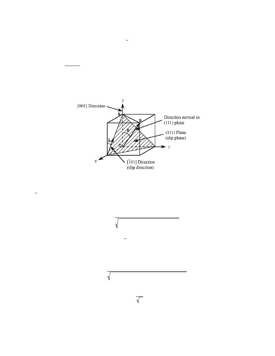
Excerpts from this work may be reproduced by instructors for distribution on a not-for-profit basis for testing or instructional purposes only to
students enrolled in courses for which the textbook has been adopted. Any other reproduction or translation of this work beyond that permitted
by Sections 107 or 108 of the 1976 United States Copyright Act without the permission of the copyright owner is unlawful.
7.14 Consider a single crystal of silver oriented such that a tensile stress is applied along a [001]
direction. If slip occurs on a (111) plane and in a
[1 01] direction, and is initiated at an applied tensile stress of 1.1
MPa (160 psi), compute the critical resolved shear stress.
Solution
This problem asks that we compute the critical resolved shear stress for silver. In order to do this, we must
employ Equation 7.4, but first it is necessary to solve for the angles
λ and φ which are shown in the sketch below.
The angle
λ is the angle between the tensile axis—i.e., along the [001] direction—and the slip direction—i.e.,
[ 1 01]. The angle
λ may be determined using Equation 7.6 as
λ = cos
−1
u
1
u
2
+ v
1
v
2
+ w
1
w
2
u
1
2
+ v
1
2
+ w
1
2
(
)
u
2
2
+ v
2
2
+ w
2
2
(
)
where (for [001]) u
1
= 0
,
v
1
= 0, w
1
= 1, and (for
[ 1 01]
) u
2
= –1, v
2
= 0, w
2
= 1. Therefore,
λ is equal to
λ = cos
−1
(0)(
−1) + (0)(0) + (1)(1)
(0)
2
+ (0)
2
+ (1)
2
[
]
(
−1)
2
+ (0)
2
+ (1)
2
[
]
= cos
−1
1
2
= 45°
Excerpts from this work may be reproduced by instructors for distribution on a not-for-profit basis for testing or instructional purposes only to
students enrolled in courses for which the textbook has been adopted. Any other reproduction or translation of this work beyond that permitted
by Sections 107 or 108 of the 1976 United States Copyright Act without the permission of the copyright owner is unlawful.
Furthermore,
φ is the angle between the tensile axis—the [001] direction—and the normal to the slip plane—i.e., the
(111) plane; for this case this normal is along a [111] direction. Therefore, again using Equation 7.6
φ = cos
−1
(0)(1)
+ (0)(1) + (1)(1)
(0)
2
+ (0)
2
+ (1)
2
[
]
(1)
2
+ (1)
2
+ (1)
2
[
]
= cos
−1
1
3
= 54.7°
And, finally, using Equation 7.4, the critical resolved shear stress is equal to
τ
crss
=
σ
y
(cos
φ cos λ)
= (1.1 MPa) cos(54.7
°) cos(45°)
[
]
= (1.1 MPa)
1
3
1
2
= 0.45 MPa (65.1 psi)
Excerpts from this work may be reproduced by instructors for distribution on a not-for-profit basis for testing or instructional purposes only to
students enrolled in courses for which the textbook has been adopted. Any other reproduction or translation of this work beyond that permitted
by Sections 107 or 108 of the 1976 United States Copyright Act without the permission of the copyright owner is unlawful.
7.15 A single crystal of a metal that has the FCC crystal structure is oriented such that a tensile stress is
applied parallel to the [110] direction. If the critical resolved shear stress for this material is 1.75 MPa, calculate
the magnitude(s) of applied stress(es) necessary to cause slip to occur on the (111) plane in each of the
[11 0],
[101 ] and
[011 ] directions.
Solution
In order to solve this problem it is necessary to employ Equation 7.4, but first we need to solve for the for
λ and φ angles for the three slip systems.
For each of these three slip systems, the
φ will be the same—i.e., the angle between the direction of the
applied stress, [110] and the normal to the (111) plane, that is, the [111] direction. The angle
φ may be determined
using Equation 7.6 as
φ = cos
−1
u
1
u
2
+ v
1
v
2
+ w
1
w
2
u
1
2
+ v
1
2
+ w
1
2
(
)
u
2
2
+ v
2
2
+ w
2
2
(
)
where (for [110]) u
1
= 1
,
v
1
= 1, w
1
= 0, and (for [111]) u
2
= 1, v
2
= 1, w
2
= 1. Therefore,
φ is equal to
φ = cos
−1
(1)(1)
+ (1)(1) + (0)(1)
(1)
2
+ (1)
2
+ (0)
2
[
]
(1)
2
+ (1)
2
+ (1)
2
[
]
= cos
−1
2
6
= 35.3°
Let us now determine
λ for the
[1 1 0 ]
slip direction. Again, using Equation 7.6 where u
1
= 1
,
v
1
= 1, w
1
= 0 (for
[110]), and u
2
= 1, v
2
= –1, w
2
= 0 (for
[11 0]. Therefore, λ is determined as
λ
[110 ]
−[1 1 0]
= cos
−1
(1)(1)
+ (1)(−1) + (0)(0)
(1)
2
+ (1)
2
+ (0)
2
[
]
(1)
2
+ (−1)
2
+ (0)
2
[
]
= cos
−1
0
= 90°
Now, we solve for the yield strength for this (111)–
[1 1 0]
slip system using Equation 7.4 as
Excerpts from this work may be reproduced by instructors for distribution on a not-for-profit basis for testing or instructional purposes only to
students enrolled in courses for which the textbook has been adopted. Any other reproduction or translation of this work beyond that permitted
by Sections 107 or 108 of the 1976 United States Copyright Act without the permission of the copyright owner is unlawful.
σ
y
=
τ
crss
(cos
φ cos λ)
=
1.75 MPa
cos (35.3
°) cos (90°)
=
1.75 MPa
(0.816) (0)
= ∞
which means that slip will not occur on this (111)–
[1 1 0] slip system.
Now, we must determine the value of
λ for the (111)–
[10 1 ] slip system—that is, the angle between the
[110] and
[10 1 ] directions. Again using Equation 7.6
λ
[110 ]
−[10 1 ]
= cos
−1
(1)(1)
+ (1)(0) + (0)(−1)
(1)
2
+ (1)
2
+ (0)
2
[
]
(1)
2
+ (0)
2
+ (−1)
2
[
]
= cos
−1
1
2
= 60°
Now, we solve for the yield strength for this (111)–
[10 1 ] slip system using Equation 7.4 as
σ
y
=
τ
crss
(cos
φ cos λ)
=
1.75 MPa
cos (35.3
°) cos (60°)
=
1.75 MPa
(0.816) (0.500)
= 4.29 MPa
And, finally, for the (111)–
[01 1 ] slip system, λ is computed using Equation 7.6 as follows:
λ
[110 ]
−[01 1 ]
= cos
−1
(1)(0)
+ (1)(1) + (0)(−1)
(1)
2
+ (1)
2
+ (0)
2
[
]
(0)
2
+ (1)
2
+ (−1)
2
[
]
= cos
−1
1
2
= 60°
Thus, since the values of
φ and λ for this (110)–
[01 1 ]
slip system are the same as for (111)–
[10 1 ]
, so also will
σ
y
be the same—viz 4.29 MPa.
Excerpts from this work may be reproduced by instructors for distribution on a not-for-profit basis for testing or instructional purposes only to
students enrolled in courses for which the textbook has been adopted. Any other reproduction or translation of this work beyond that permitted
by Sections 107 or 108 of the 1976 United States Copyright Act without the permission of the copyright owner is unlawful.
7.16 (a) A single crystal of a metal that has the BCC crystal structure is oriented such that a tensile stress
is applied in the [010] direction. If the magnitude of this stress is 2.75 MPa, compute the resolved shear stress in the
[1 11] direction on each of the (110) and (101) planes.
(b) On the basis of these resolved shear stress values, which slip system(s) is (are) most favorably
oriented?
Solution
(a) This part of the problem asks, for a BCC metal, that we compute the resolved shear stress in the
[ 1 11 ]
direction on each of the (110) and (101) planes. In order to solve this problem it is necessary to employ Equation
7.2, which means that we first need to solve for the for angles
λ and φ for the three slip systems.
For each of these three slip systems, the
λ will be the same—i.e., the angle between the direction of the
applied stress, [010] and the slip direction,
[ 1 11]. This angle
λ may be determined using Equation 7.6
λ = cos
−1
u
1
u
2
+ v
1
v
2
+ w
1
w
2
u
1
2
+ v
1
2
+ w
1
2
(
)
u
2
2
+ v
2
2
+ w
2
2
(
)
where (for [010]) u
1
= 0
,
v
1
= 1, w
1
= 0, and (for
[ 1 11]) u
2
= –1, v
2
= 1, w
2
= 1. Therefore,
λ is determined as
λ = cos
−1
(0)(
−1) + (1)(1) + (0)(1)
(0)
2
+ (1)
2
+ (0)
2
[
]
(
−1)
2
+ (1)
2
+ (1)
2
[
]
= cos
−1
1
3
= 54.7°
Let us now determine
φ for the angle between the direction of the applied tensile stress—i.e., the [010] direction—
and the normal to the (110) slip plane—i.e., the [110] direction. Again, using Equation 7.6 where u
1
= 0
,
v
1
= 1, w
1
= 0 (for [010]), and u
2
= 1, v
2
= 1, w
2
= 0 (for [110]),
φ is equal to
φ
[010 ]
−[110]
= cos
−1
(0)(1)
+ (1)(1) + (0)(0)
(0)
2
+ (1)
2
+ (0)
2
[
]
(1)
2
+ (1)
2
+ (0)
2
[
]
= cos
−1
1
2
= 45°
Excerpts from this work may be reproduced by instructors for distribution on a not-for-profit basis for testing or instructional purposes only to
students enrolled in courses for which the textbook has been adopted. Any other reproduction or translation of this work beyond that permitted
by Sections 107 or 108 of the 1976 United States Copyright Act without the permission of the copyright owner is unlawful.
Now, using Equation 7.2
τ
R
= σ cosφ cos λ
we solve for the resolved shear stress for this slip system as
τ
R(110)
−[1 11]
= (2.75 MPa) cos (54.7°) cos (45°)
[
]
= (2.75 MPa) (0.578)(0.707) = 1.12 MPa
Now, we must determine the value of
φ for the (101)–
[ 1 11] slip system—that is, the angle between the
direction of the applied stress, [010], and the normal to the (101) plane—i.e., the [101] direction. Again using
Equation 7.6
λ
[010 ]
−[101]
= cos
−1
(0)(1)
+ (1)(0) + (0)(1)
(0)
2
+ (1)
2
+ (0)
2
[
]
(1)
2
+ (0)
2
+ (1)
2
[
]
= cos
−1
(0)
= 90°
Thus, the resolved shear stress for this (101)–
[ 1 11] slip system is
τ
R(101)
−[1 11]
= = (2.75 MPa) cos (54.7°) cos (90°)
[
]
= (2.75 MPa) (0.578)(0) = 0 MPa
(b) The most favored slip system(s) is (are) the one(s) that has (have) the largest
τ
R
value. Therefore, the
(110)–
[ 1 11 ] is the most favored since its τ
R
(1.12 MPa) is greater than the
τ
R
value for
(101)
−[1 11] (viz., 0
MPa).
Excerpts from this work may be reproduced by instructors for distribution on a not-for-profit basis for testing or instructional purposes only to
students enrolled in courses for which the textbook has been adopted. Any other reproduction or translation of this work beyond that permitted
by Sections 107 or 108 of the 1976 United States Copyright Act without the permission of the copyright owner is unlawful.
7.17 Consider a single crystal of some hypothetical metal that has the FCC crystal structure and is
oriented such that a tensile stress is applied along a
[1 02] direction. If slip occurs on a (111) plane and in a
[1 01]
direction, compute the stress at which the crystal yields if its critical resolved shear stress is 3.42 MPa.
Solution
This problem asks for us to determine the tensile stress at which a FCC metal yields when the stress is
applied along a
[ 1 02] direction such that slip occurs on a (111) plane and in a
[ 1 01] direction; the critical resolved
shear stress for this metal is 3.42 MPa. To solve this problem we use Equation 7.4; however it is first necessary to
determine the values of
φ and λ. These determinations are possible using Equation 7.6. Now, λ is the angle
between
[ 1 02] and
[ 1 01 ] directions. Therefore, relative to Equation 7.6 let us take u
1
= –1, v
1
= 0, and w
1
= 2, as
well as u
2
= –1, v
2
= 0, and w
2
= 1. This leads to
λ = cos
−1
u
1
u
2
+ v
1
v
2
+ w
1
w
2
u
1
2
+ v
1
2
+ w
1
2
(
)
u
2
2
+ v
2
2
+ w
2
2
(
)
= cos
−1
(
−1)(−1) + (0)(0) + (2)(1)
(
−1)
2
+ (0)
2
+ (2)
2
[
]
(
−1)
2
+ (0)
2
+ (1)
2
[
]
= cos
−1
3
10
= 18.4°
Now for the determination of
φ, the normal to the (111) slip plane is the [111] direction. Again using Equation 7.6,
where we now take u
1
= –1, v
1
= 0, w
1
= 2 (for
[ 1 02] ), and u
2
= 1, v
2
= 1, w
2
= 1 (for [111]). Thus,
φ = cos
−1
(
−1)(1) + (0)(1) + (2)(1)
(
−1)
2
+ (0)
2
+ (2)
2
[
]
(1)
2
+ (1)
2
+ (1)
2
[
]
= cos
−1
3
15
= 39.2°
It is now possible to compute the yield stress (using Equation 7.4) as

Excerpts from this work may be reproduced by instructors for distribution on a not-for-profit basis for testing or instructional purposes only to
students enrolled in courses for which the textbook has been adopted. Any other reproduction or translation of this work beyond that permitted
by Sections 107 or 108 of the 1976 United States Copyright Act without the permission of the copyright owner is unlawful.
σ
y
=
τ
crss
cos
φ cos λ
=
3.42 MPa
3
10
3
15
= 4.65 MPa

Excerpts from this work may be reproduced by instructors for distribution on a not-for-profit basis for testing or instructional purposes only to
students enrolled in courses for which the textbook has been adopted. Any other reproduction or translation of this work beyond that permitted
by Sections 107 or 108 of the 1976 United States Copyright Act without the permission of the copyright owner is unlawful.
7.18 The critical resolved shear stress for iron is 27 MPa (4000 psi). Determine the maximum possible
yield strength for a single crystal of Fe pulled in tension.
Solution
In order to determine the maximum possible yield strength for a single crystal of Fe pulled in tension, we
simply employ Equation 7.5 as
σ
y
= 2
τ
crss
= (2)(27 MPa) = 54 MPa (8000 psi)

Excerpts from this work may be reproduced by instructors for distribution on a not-for-profit basis for testing or instructional purposes only to
students enrolled in courses for which the textbook has been adopted. Any other reproduction or translation of this work beyond that permitted
by Sections 107 or 108 of the 1976 United States Copyright Act without the permission of the copyright owner is unlawful.
Deformation by Twinning
7.19 List four major differences between deformation by twinning and deformation by slip relative to
mechanism, conditions of occurrence, and final result.
Solution
Four major differences between deformation by twinning and deformation by slip are as follows: (1) with
slip deformation there is no crystallographic reorientation, whereas with twinning there is a reorientation; (2) for
slip, the atomic displacements occur in atomic spacing multiples, whereas for twinning, these displacements may be
other than by atomic spacing multiples; (3) slip occurs in metals having many slip systems, whereas twinning
occurs in metals having relatively few slip systems; and (4) normally slip results in relatively large deformations,
whereas only small deformations result for twinning.

Excerpts from this work may be reproduced by instructors for distribution on a not-for-profit basis for testing or instructional purposes only to
students enrolled in courses for which the textbook has been adopted. Any other reproduction or translation of this work beyond that permitted
by Sections 107 or 108 of the 1976 United States Copyright Act without the permission of the copyright owner is unlawful.
Strengthening by Grain Size Reduction
7.20 Briefly explain why small-angle grain boundaries are not as effective in interfering with the slip
process as are high-angle grain boundaries.
Solution
Small-angle grain boundaries are not as effective in interfering with the slip process as are high-angle grain
boundaries because there is not as much crystallographic misalignment in the grain boundary region for small-angle,
and therefore not as much change in slip direction.

Excerpts from this work may be reproduced by instructors for distribution on a not-for-profit basis for testing or instructional purposes only to
students enrolled in courses for which the textbook has been adopted. Any other reproduction or translation of this work beyond that permitted
by Sections 107 or 108 of the 1976 United States Copyright Act without the permission of the copyright owner is unlawful.
7.21 Briefly explain why HCP metals are typically more brittle than FCC and BCC metals.
Solution
Hexagonal close packed metals are typically more brittle than FCC and BCC metals because there are
fewer slip systems in HCP.

Excerpts from this work may be reproduced by instructors for distribution on a not-for-profit basis for testing or instructional purposes only to
students enrolled in courses for which the textbook has been adopted. Any other reproduction or translation of this work beyond that permitted
by Sections 107 or 108 of the 1976 United States Copyright Act without the permission of the copyright owner is unlawful.
7.22 Describe in your own words the three strengthening mechanisms discussed in this chapter (i.e., grain
size reduction, solid-solution strengthening, and strain hardening). Be sure to explain how dislocations are involved
in each of the strengthening techniques.
These three strengthening mechanisms are described in Sections 7.8, 7.9, and 7.10.

Excerpts from this work may be reproduced by instructors for distribution on a not-for-profit basis for testing or instructional purposes only to
students enrolled in courses for which the textbook has been adopted. Any other reproduction or translation of this work beyond that permitted
by Sections 107 or 108 of the 1976 United States Copyright Act without the permission of the copyright owner is unlawful.
7.23 (a) From the plot of yield strength versus (grain diameter)
–1/2
for a 70 Cu–30 Zn cartridge brass,
Figure 7.15, determine values for the constants σ
0
and k
y
in Equation 7.7.
(b) Now predict the yield strength of this alloy when the average grain diameter is 1.0
× 10
-3
mm.
Solution
(a) Perhaps the easiest way to solve for
σ
0
and k
y
in Equation 7.7 is to pick two values each of
σ
y
and d
-1/2
from Figure 7.15, and then solve two simultaneous equations, which may be created. For example
d
-1/2
(mm)
-1/2
σ
y
(MPa)
4
75
12
175
The two equations are thus
75 =
σ
0
+ 4 k
y
175 =
σ
0
+ 12 k
y
Solution of these equations yield the values of
k
y
= 12.5 MPa (mm)
1/2
1810 psi (mm)
1/2
[
]
σ
0
= 25 MPa (3630 psi)
(b) When d = 1.0
× 10
-3
mm, d
-1/2
= 31.6 mm
-1/2
, and, using Equation 7.7,
σ
y
=
σ
0
+ k
y
d
-1/2
= (25 MPa) + 12.5 MPa (mm)
1/2
(
31.6 mm
-1/2
)
= 420 MPa (61, 000 psi)

Excerpts from this work may be reproduced by instructors for distribution on a not-for-profit basis for testing or instructional purposes only to
students enrolled in courses for which the textbook has been adopted. Any other reproduction or translation of this work beyond that permitted
by Sections 107 or 108 of the 1976 United States Copyright Act without the permission of the copyright owner is unlawful.
7.24 The lower yield point for an iron that has an average grain diameter of 5
× 10
-2
mm is 135 MPa
(19,500 psi). At a grain diameter of 8
× 10
-3
mm, the yield point increases to 260 MPa (37,500 psi). At what grain
diameter will the lower yield point be 205 MPa (30,000 psi)?
Solution
The best way to solve this problem is to first establish two simultaneous expressions of Equation 7.7, solve
for
σ
0
and k
y
, and finally determine the value of d when
σ
y
= 205 MPa. The data pertaining to this problem may be
tabulated as follows:
σ
y
d (mm)
d
-1/2
(mm)
-1/2
135 MPa
5
× 10
-2
4.47
260 MPa
8
× 10
-3
11.18
The two equations thus become
135 MPa =
σ
0
+ (4.47) k
y
260 MPa =
σ
0
+ (11.18) k
y
Which yield the values,
σ
0
= 51.7 MPa and ky = 18.63 MPa(mm)
1/2
. At a yield strength of 205 MPa
205 MPa = 51.7 MPa + 18.63 MPa (mm)
1/2
[
]
d
-1/2
or d
-1/2
= 8.23 (mm)
-1/2
, which gives d = 1.48
× 10
-2
mm.

Excerpts from this work may be reproduced by instructors for distribution on a not-for-profit basis for testing or instructional purposes only to
students enrolled in courses for which the textbook has been adopted. Any other reproduction or translation of this work beyond that permitted
by Sections 107 or 108 of the 1976 United States Copyright Act without the permission of the copyright owner is unlawful.
7.25 If it is assumed that the plot in Figure 7.15 is for noncold-worked brass, determine the grain size of
the alloy in Figure 7.19; assume its composition is the same as the alloy in Figure 7.15.
Solution
This problem asks that we determine the grain size of the brass for which is the subject of Figure 7.19.
From Figure 7.19a, the yield strength of brass at 0%CW is approximately 175 MPa (26,000 psi). This yield
strength from Figure 7.15 corresponds to a d
-1/2
value of approximately 12.0 (mm)
-1/2
. Thus, d = 6.9
× 10
-3
mm.
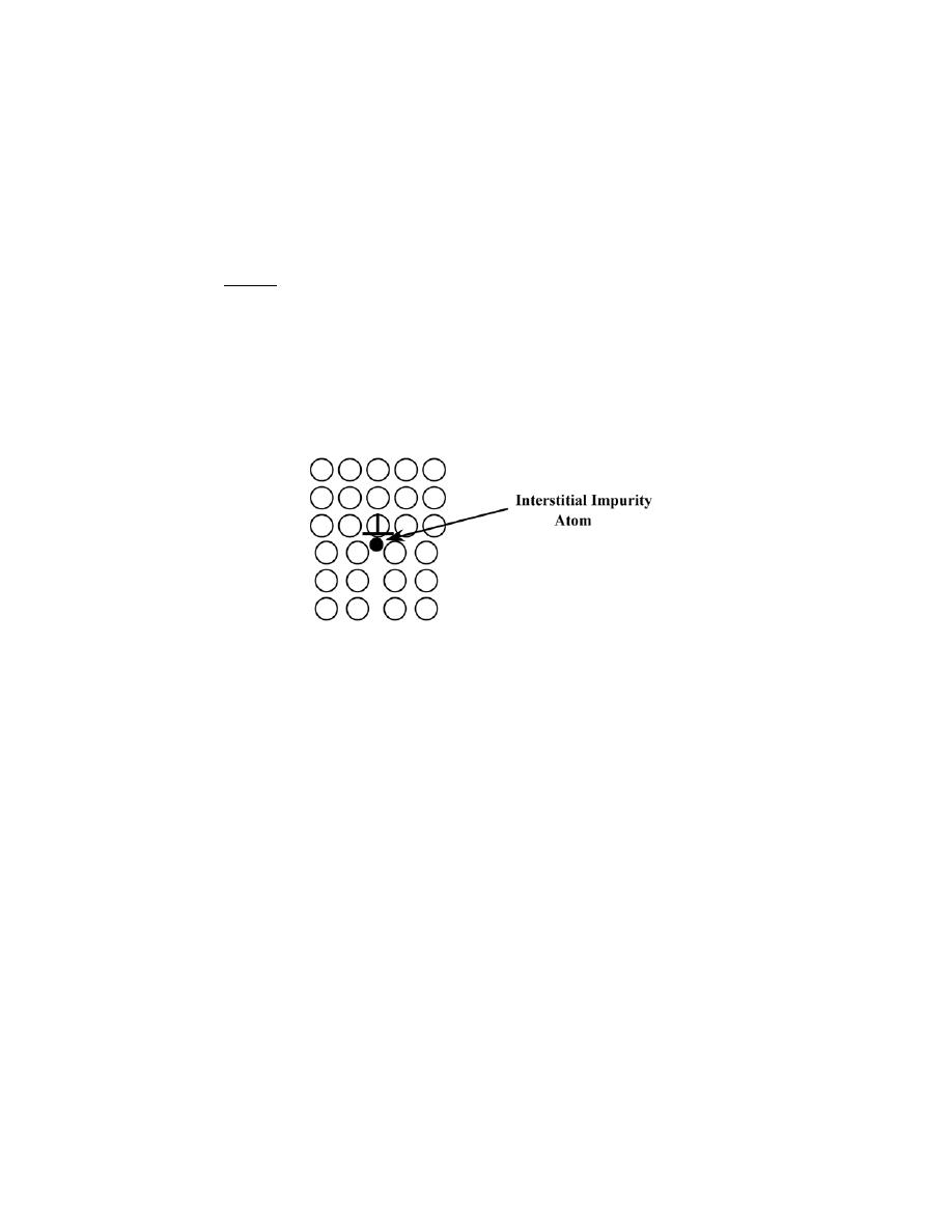
Excerpts from this work may be reproduced by instructors for distribution on a not-for-profit basis for testing or instructional purposes only to
students enrolled in courses for which the textbook has been adopted. Any other reproduction or translation of this work beyond that permitted
by Sections 107 or 108 of the 1976 United States Copyright Act without the permission of the copyright owner is unlawful.
Solid-Solution Strengthening
7.26 In the manner of Figures 7.17b and 7.18b, indicate the location in the vicinity of an edge dislocation
at which an interstitial impurity atom would be expected to be situated. Now briefly explain in terms of lattice
strains why it would be situated at this position.
Solution
Below is shown an edge dislocation and where an interstitial impurity atom would be located.
Compressive lattice strains are introduced by the impurity atom. There will be a net reduction in lattice strain
energy when these lattice strains partially cancel tensile strains associated with the edge dislocation; such tensile
strains exist just below the bottom of the extra half-plane of atoms (Figure 7.4).

Excerpts from this work may be reproduced by instructors for distribution on a not-for-profit basis for testing or instructional purposes only to
students enrolled in courses for which the textbook has been adopted. Any other reproduction or translation of this work beyond that permitted
by Sections 107 or 108 of the 1976 United States Copyright Act without the permission of the copyright owner is unlawful.
Strain Hardening
7.27 (a) Show, for a tensile test, that
%CW
=
ε
ε+1
×100
if there is no change in specimen volume during the deformation process (i.e., A
0
l
0
= A
d
l
d
).
(b) Using the result of part (a), compute the percent cold work experienced by naval brass (the stress-
strain behavior of which is shown in Figure 6.12) when a stress of 400 MPa (58,000 psi) is applied.
Solution
(a) From Equation 7.8
%CW =
A
0
− A
d
A
0
× 100 = 1 −
A
d
A
0
× 100
Which is also equal to
1
−
l
0
l
d
× 100
since A
d
/A
0
= l
0
/l
d
, the conservation of volume stipulation given in the problem statement. Now, from the definition
of engineering strain (Equation 6.2)
ε =
l
d
− l
0
l
0
=
l
d
l
0
−1
Or,
l
0
l
d
=
1
ε + 1
Substitution for l
0
/ l
d
into the %CW expression above gives
%CW = 1
−
l
0
l
d
× 100 = 1 −
1
ε + 1
× 100 =
ε
ε + 1
× 100

Excerpts from this work may be reproduced by instructors for distribution on a not-for-profit basis for testing or instructional purposes only to
students enrolled in courses for which the textbook has been adopted. Any other reproduction or translation of this work beyond that permitted
by Sections 107 or 108 of the 1976 United States Copyright Act without the permission of the copyright owner is unlawful.
(b) From Figure 6.12, a stress of 400 MPa (58,000 psi) corresponds to a strain of 0.13. Using the above
expression
%CW =
ε
ε + 1
× 100 =
0.13
0.13
+ 1.00
× 100 = 11.5%CW
Excerpts from this work may be reproduced by instructors for distribution on a not-for-profit basis for testing or instructional purposes only to
students enrolled in courses for which the textbook has been adopted. Any other reproduction or translation of this work beyond that permitted
by Sections 107 or 108 of the 1976 United States Copyright Act without the permission of the copyright owner is unlawful.
7.28 Two previously undeformed cylindrical specimens of an alloy are to be strain hardened by reducing
their cross-sectional areas (while maintaining their circular cross sections). For one specimen, the initial and
deformed radii are 16 mm and 11 mm, respectively. The second specimen, with an initial radius of 12 mm, must
have the same deformed hardness as the first specimen; compute the second specimen's radius after deformation.
Solution
In order for these two cylindrical specimens to have the same deformed hardness, they must be deformed
to the same percent cold work. For the first specimen
%CW =
A
0
− A
d
A
0
× 100 =
π r
0
2
− π r
d
2
π r
0
2
× 100
=
π (16 mm)
2
− π (11 mm)
2
π (16 mm)
2
× 100 = 52.7%CW
For the second specimen, the deformed radius is computed using the above equation and solving for r
d
as
r
d
= r
0
1
−
%CW
100
= (12 mm) 1
−
52.7%CW
100
= 8.25 mm

Excerpts from this work may be reproduced by instructors for distribution on a not-for-profit basis for testing or instructional purposes only to
students enrolled in courses for which the textbook has been adopted. Any other reproduction or translation of this work beyond that permitted
by Sections 107 or 108 of the 1976 United States Copyright Act without the permission of the copyright owner is unlawful.
7.29 Two previously undeformed specimens of the same metal are to be plastically deformed by reducing
their cross-sectional areas. One has a circular cross section, and the other is rectangular; during deformation the
circular cross section is to remain circular, and the rectangular is to remain as such. Their original and deformed
dimensions are as follows:
Circular (diameter, mm)
Rectangular (mm)
Original dimensions
15.2
125 × 175
Deformed dimensions
11.4
75 × 200
Which of these specimens will be the hardest after plastic deformation, and why?
Solution
The hardest specimen will be the one that has experienced the greatest degree of cold work. Therefore, all
we need do is to compute the %CW for each specimen using Equation 7.8. For the circular one
%CW =
A
0
− A
d
A
0
× 100
=
π r
0
2
− π r
d
2
π r
0
2
× 100
=
π
15.2 mm
2
2
− π
11.4 mm
2
2
π
15.2 mm
2
2
× 100 = 43.8%CW
For the rectangular one
%CW =
(125 mm)(175 mm)
− (75 mm)(200 mm)
(125 mm)(175 mm)
× 100 = 31.4%CW
Therefore, the deformed circular specimen will be harder.
Excerpts from this work may be reproduced by instructors for distribution on a not-for-profit basis for testing or instructional purposes only to
students enrolled in courses for which the textbook has been adopted. Any other reproduction or translation of this work beyond that permitted
by Sections 107 or 108 of the 1976 United States Copyright Act without the permission of the copyright owner is unlawful.
7.30 A cylindrical specimen of cold-worked copper has a ductility (%EL) of 25%. If its cold-worked
radius is 10 mm (0.40 in.), what was its radius before deformation?
Solution
This problem calls for us to calculate the precold-worked radius of a cylindrical specimen of copper that
has a cold-worked ductility of 25%EL. From Figure 7.19c, copper that has a ductility of 25%EL will have
experienced a deformation of about 11%CW. For a cylindrical specimen, Equation 7.8 becomes
%CW =
π r
0
2
− π r
d
2
π r
0
2
× 100
Since r
d
= 10 mm (0.40 in.), solving for r
0
yields
r
0
=
r
d
1
−
%CW
100
=
10 mm
1
−
11.0
100
= 10.6 mm (0.424 in.)

Excerpts from this work may be reproduced by instructors for distribution on a not-for-profit basis for testing or instructional purposes only to
students enrolled in courses for which the textbook has been adopted. Any other reproduction or translation of this work beyond that permitted
by Sections 107 or 108 of the 1976 United States Copyright Act without the permission of the copyright owner is unlawful.
7.31 (a) What is the approximate ductility (%EL) of a brass that has a yield strength of 275 MPa (40,000
psi)?
(b) What is the approximate Brinell hardness of a 1040 steel having a yield strength of 690 MPa (100,000
psi)?
Solution
(a) In order to solve this problem, it is necessary to consult Figures 7.19a and 7.19c. From Figure 7.19a, a
yield strength of 275 MPa for brass corresponds to 10%CW. A brass that has been cold-worked 10% will have a
ductility of about 43%EL [Figure 7.19c].
(b) This portion of the problem asks for the Brinell hardness of a 1040 steel having a yield strength of 690
MPa (100,000 psi). From Figure 7.19a, a yield strength of 690 MPa for a 1040 steel corresponds to about 10%CW.
A 1040 steel that has been cold worked 10% will have a tensile strength of about 780 MPa [Figure 7.19b]. Finally,
using Equation 6.20a
HB =
TS (MPa)
3.45
=
780 MPa
3.45
= 226
Excerpts from this work may be reproduced by instructors for distribution on a not-for-profit basis for testing or instructional purposes only to
students enrolled in courses for which the textbook has been adopted. Any other reproduction or translation of this work beyond that permitted
by Sections 107 or 108 of the 1976 United States Copyright Act without the permission of the copyright owner is unlawful.
7.32 Experimentally, it has been observed for single crystals of a number of metals that the critical
resolved shear stress
τ
crss
is a function of the dislocation density ρ
D
as
τ
crss
= τ
0
+ A ρ
D
where τ
0
and A are constants. For copper, the critical resolved shear stress is 2.10 MPa (305 psi) at a dislocation
density of 10
5
mm
-2
. If it is known that the value of A for copper is 6.35
× 10
-3
MPa-mm (0.92 psi-mm), compute the
τ
crss
at a dislocation density of 10
7
mm
-2
.
Solution
We are asked in this problem to compute the critical resolved shear stress at a dislocation density of 10
7
mm
-2
. It is first necessary to compute the value of the constant
τ
0
(in the equation provided in the problem
statement) from the one set of data as
τ
0
= τ
crss
− A ρ
D
= 2.10 MPa −
(
6.35
× 10
−3
MPa - mm
)
10
5
mm
−2
(
)
= 0.092 MPa (13.3 psi)
Now, the critical resolved shear stress may be determined at a dislocation density of 10
7
mm
-2
as
τ
crss
=
τ
0
+ A
ρ
D
= (0.092 MPa) +
(
6.35
× 10
-3
MPa - mm
)
10
7
mm
−2
= 20.2 MPa (2920 psi)

Excerpts from this work may be reproduced by instructors for distribution on a not-for-profit basis for testing or instructional purposes only to
students enrolled in courses for which the textbook has been adopted. Any other reproduction or translation of this work beyond that permitted
by Sections 107 or 108 of the 1976 United States Copyright Act without the permission of the copyright owner is unlawful.
Recovery
Recrystallization
Grain Growth
7.33 Briefly cite the differences between recovery and recrystallization processes.
Solution
For recovery, there is some relief of internal strain energy by dislocation motion; however, there are
virtually no changes in either the grain structure or mechanical characteristics. During recrystallization, on the other
hand, a new set of strain-free grains forms, and the material becomes softer and more ductile.
Excerpts from this work may be reproduced by instructors for distribution on a not-for-profit basis for testing or instructional purposes only to
students enrolled in courses for which the textbook has been adopted. Any other reproduction or translation of this work beyond that permitted
by Sections 107 or 108 of the 1976 United States Copyright Act without the permission of the copyright owner is unlawful.
7.34 Estimate the fraction of recrystallization from the photomicrograph in Figure 7.21c.
Solution
Below is shown a square grid onto which is superimposed the recrystallized regions from the micrograph.
Approximately 400 squares lie within the recrystallized areas, and since there are 672 total squares, the specimen is
about 60% recrystallized.

Excerpts from this work may be reproduced by instructors for distribution on a not-for-profit basis for testing or instructional purposes only to
students enrolled in courses for which the textbook has been adopted. Any other reproduction or translation of this work beyond that permitted
by Sections 107 or 108 of the 1976 United States Copyright Act without the permission of the copyright owner is unlawful.
7.35 Explain the differences in grain structure for a metal that has been cold worked and one that has
been cold worked and then recrystallized.
Solution
During cold-working, the grain structure of the metal has been distorted to accommodate the deformation.
Recrystallization produces grains that are equiaxed and smaller than the parent grains.

Excerpts from this work may be reproduced by instructors for distribution on a not-for-profit basis for testing or instructional purposes only to
students enrolled in courses for which the textbook has been adopted. Any other reproduction or translation of this work beyond that permitted
by Sections 107 or 108 of the 1976 United States Copyright Act without the permission of the copyright owner is unlawful.
7.36 (a) What is the driving force for recrystallization?
(b) For grain growth?
Solution
(a) The driving force for recrystallization is the difference in internal energy between the strained and
unstrained material.
(b) The driving force for grain growth is the reduction in grain boundary energy as the total grain
boundary area decreases.

Excerpts from this work may be reproduced by instructors for distribution on a not-for-profit basis for testing or instructional purposes only to
students enrolled in courses for which the textbook has been adopted. Any other reproduction or translation of this work beyond that permitted
by Sections 107 or 108 of the 1976 United States Copyright Act without the permission of the copyright owner is unlawful.
7.37 (a) From Figure 7.25, compute the length of time required for the average grain diameter to increase
from 0.01 to 0.1 mm at 500
°C for this brass material.
(b) Repeat the calculation at 600°C.
Solution
(a) At 500
°C, the time necessary for the average grain diameter to grow to increase from 0.01 to 0.1 mm is
approximately 3500 min.
(b) At 600
°C the time required for this same grain size increase is approximately 150 min.
Excerpts from this work may be reproduced by instructors for distribution on a not-for-profit basis for testing or instructional purposes only to
students enrolled in courses for which the textbook has been adopted. Any other reproduction or translation of this work beyond that permitted
by Sections 107 or 108 of the 1976 United States Copyright Act without the permission of the copyright owner is unlawful.
7.38 The average grain diameter for a brass material was measured as a function of time at 650°C, which
is tabulated below at two different times:
Time (min)
Grain Diameter (mm)
30
3.9 × 10
–2
90
6.6 × 10
–2
(a) What was the original grain diameter?
(b) What grain diameter would you predict after 150 min at 650°C?
Solution
(a) Using the data given and Equation 7.9 (taking n = 2), we may set up two simultaneous equations with
d
0
and K as unknowns; thus
(
3.9
× 10
-2
mm
)
2
− d
0
2
= (30 min) K
(
6.6
× 10
-2
mm
)
2
− d
0
2
= (90 min) K
Solution of these expressions yields a value for d
0
, the original grain diameter, of
d
0
= 0.01 mm,
and a value for K of 4.73
× 10
-5
mm
2
/min
(b) At 150 min, the diameter d is computed using a rearranged form of Equation 7.9 as
d =
d
0
2
+ Kt
=
(0.01 mm)
2
+
(
4.73
× 10
−5
mm
2
/min
)
(150 min) = 0.085 mm

Excerpts from this work may be reproduced by instructors for distribution on a not-for-profit basis for testing or instructional purposes only to
students enrolled in courses for which the textbook has been adopted. Any other reproduction or translation of this work beyond that permitted
by Sections 107 or 108 of the 1976 United States Copyright Act without the permission of the copyright owner is unlawful.
7.39 An undeformed specimen of some alloy has an average grain diameter of 0.040 mm. You are asked
to reduce its average grain diameter to 0.010 mm. Is this possible? If so, explain the procedures you would use
and name the processes involved. If it is not possible, explain why.
Solution
Yes, it is possible to reduce the average grain diameter of an undeformed alloy specimen from 0.040 mm to
0.010 mm. In order to do this, plastically deform the material at room temperature (i.e., cold work it), and then
anneal at an elevated temperature in order to allow recrystallization and some grain growth to occur until the
average grain diameter is 0.010 mm.

Excerpts from this work may be reproduced by instructors for distribution on a not-for-profit basis for testing or instructional purposes only to
students enrolled in courses for which the textbook has been adopted. Any other reproduction or translation of this work beyond that permitted
by Sections 107 or 108 of the 1976 United States Copyright Act without the permission of the copyright owner is unlawful.
7.40 Grain growth is strongly dependent on temperature (i.e., rate of grain growth increases with
increasing temperature), yet temperature is not explicitly given as a part of Equation 7.9.
(a) Into which of the parameters in this expression would you expect temperature to be included?
(b) On the basis of your intuition, cite an explicit expression for this temperature dependence.
Solution
(a) The temperature dependence of grain growth is incorporated into the constant K in Equation 7.9.
(b) The explicit expression for this temperature dependence is of the form
K = K
0
exp
−
Q
RT
in which K
0
is a temperature-independent constant, the parameter Q is an activation energy, and R and T are the gas
constant and absolute temperature, respectively.

Excerpts from this work may be reproduced by instructors for distribution on a not-for-profit basis for testing or instructional purposes only to
students enrolled in courses for which the textbook has been adopted. Any other reproduction or translation of this work beyond that permitted
by Sections 107 or 108 of the 1976 United States Copyright Act without the permission of the copyright owner is unlawful.
7.41 An uncold-worked brass specimen of average grain size 0.008 mm has a yield strength of 160 MPa
(23,500 psi). Estimate the yield strength of this alloy after it has been heated to 600
°C for 1000 s, if it is known that
the value of k
y
is 12.0 MPa-mm
1/2
(1740 psi-mm
1/2
).
Solution
In order to solve this problem, it is first necessary to calculate the constant
σ
0
in Equation 7.7 as
σ
0
=
σ
y
− k
y
d
-1/2
= 160 MPa
−
(
12.0 MPa
− mm
1/2
)
(0.008 mm)
−1/ 2
= 25.8 MPa (4046 psi)
Next, we must determine the average grain size after the heat treatment. From Figure 7.25 at 600
°C after 1000 s
(16.7 min) the average grain size of a brass material is about 0.20 mm. Therefore, calculating
σ
y
at this new grain
size using Equation 7.7 we get
σ
y
=
σ
0
+ k
y
d
-1/2
= 25.8 MPa
+
(
12.0 MPa - mm
1/2
)
(0.20 mm)
-1/2
= 52.6 MPa (7940 psi)

Excerpts from this work may be reproduced by instructors for distribution on a not-for-profit basis for testing or instructional purposes only to
students enrolled in courses for which the textbook has been adopted. Any other reproduction or translation of this work beyond that permitted
by Sections 107 or 108 of the 1976 United States Copyright Act without the permission of the copyright owner is unlawful.
DESIGN PROBLEMS
Strain Hardening
Recrystallization
7.D1 Determine whether or not it is possible to cold work steel so as to give a minimum Brinell hardness
of 225, and at the same time have a ductility of at least 12%EL. Justify your decision.
Solution
The tensile strength corresponding to a Brinell hardness of 225 may be determined using Equation 6.20a as
TS(MPa)
= 3.45 × HB = (3.45)(225) = 776 MPa
Furthermore, from Figure 7.19b, in order to achieve a tensile strength of 776 MPa, deformation of at least 9%CW is
necessary. Finally, if we cold work the steel to 9%CW, then the ductility is 17%EL from Figure 7.19c. Therefore,
it is possible to meet both of these criteria by plastically deforming the steel.

Excerpts from this work may be reproduced by instructors for distribution on a not-for-profit basis for testing or instructional purposes only to
students enrolled in courses for which the textbook has been adopted. Any other reproduction or translation of this work beyond that permitted
by Sections 107 or 108 of the 1976 United States Copyright Act without the permission of the copyright owner is unlawful.
7.D2 Determine whether or not it is possible to cold work brass so as to give a minimum Brinell hardness
of 120 and at the same time have a ductility of at least 20%EL. Justify your decision.
Solution
According to Figure 6.19, a Brinell hardness of 120 corresponds to a tensile strength of 440 MPa (63,500
psi.) Furthermore, from Figure 7.19b, in order to achieve a tensile strength of 440 MPa, deformation of at least
26%CW is necessary. Finally, if we are to achieve a ductility of at least 20%EL, then a maximum deformation of
23%CW is possible from Figure 7.19c. Therefore, it is not possible to meet both of these criteria by plastically
deforming brass.

Excerpts from this work may be reproduced by instructors for distribution on a not-for-profit basis for testing or instructional purposes only to
students enrolled in courses for which the textbook has been adopted. Any other reproduction or translation of this work beyond that permitted
by Sections 107 or 108 of the 1976 United States Copyright Act without the permission of the copyright owner is unlawful.
7.D3 A cylindrical specimen of cold-worked steel has a Brinell hardness of 250.
(a) Estimate its ductility in percent elongation.
(b) If the specimen remained cylindrical during deformation and its original radius was 5 mm (0.20 in.),
determine its radius after deformation.
Solution
(a) From Figure 6.19, a Brinell hardness of 250 corresponds to a tensile strength of 860 MPa (125,000
psi), which, from Figure 7.19b, requires a deformation of 25%CW. Furthermore, 25%CW yields a ductility of
about 11%EL for steel, Figure 7.19c.
(b) We are now asked to determine the radius after deformation if the uncold-worked radius is 5 mm (0.20
in.). From Equation 7.8 and for a cylindrical specimen
%CW =
π r
0
2
− π r
d
2
π r
0
2
× 100
Now, solving for r
d
from this expression, we get
r
d
= r
0
1
−
%CW
100
= (5 mm)
1
−
25
100
= 4.33 mm (0.173 in.)

Excerpts from this work may be reproduced by instructors for distribution on a not-for-profit basis for testing or instructional purposes only to
students enrolled in courses for which the textbook has been adopted. Any other reproduction or translation of this work beyond that permitted
by Sections 107 or 108 of the 1976 United States Copyright Act without the permission of the copyright owner is unlawful.
7.D4 It is necessary to select a metal alloy for an application that requires a yield strength of at least 345
MPa (50,000 psi) while maintaining a minimum ductility (%EL) of 20%. If the metal may be cold worked, decide
which of the following are candidates: copper, brass, and a 1040 steel. Why?
Solution
For each of these alloys, the minimum cold work necessary to achieve the yield strength may be
determined from Figure 7.19a, while the maximum possible cold work for the ductility is found in Figure 7.19c.
These data are tabulated below.
Yield Strength
Ductility
(> 345 MPa)
(> 20%EL)
Steel
Any %CW
< 5%CW
Brass
> 20%CW
< 23%CW
Copper
> 54%CW
< 15%CW
Thus, both the 1040 steel and brass are possible candidates since for these alloys there is an overlap of percents
coldwork to give the required minimum yield strength and ductility values.

Excerpts from this work may be reproduced by instructors for distribution on a not-for-profit basis for testing or instructional purposes only to
students enrolled in courses for which the textbook has been adopted. Any other reproduction or translation of this work beyond that permitted
by Sections 107 or 108 of the 1976 United States Copyright Act without the permission of the copyright owner is unlawful.
7.D5 A cylindrical rod of 1040 steel originally 15.2 mm (0.60 in.) in diameter is to be cold worked by
drawing; the circular cross section will be maintained during deformation. A cold-worked tensile strength in
excess of 840 MPa (122,000 psi) and a ductility of at least 12%EL are desired. Furthermore, the final diameter
must be 10 mm (0.40 in.). Explain how this may be accomplished.
Solution
First let us calculate the percent cold work and attendant tensile strength and ductility if the drawing is
carried out without interruption. From Equation 7.8
%CW =
π
d
0
2
2
− π
d
d
2
2
π
d
0
2
2
× 100
=
π
15.2 mm
2
2
− π
10 mm
2
2
π
15.2 mm
2
2
× 100 = 56%CW
At 56%CW, the steel will have a tensile strength on the order of 920 MPa (133,000 psi) [Figure 7.19b], which is
adequate; however, the ductility will be less than 10%EL [Figure 7.19c], which is insufficient.
Instead of performing the drawing in a single operation, let us initially draw some fraction of the total
deformation, then anneal to recrystallize, and, finally, cold-work the material a second time in order to achieve the
final diameter, tensile strength, and ductility.
Reference to Figure 7.19b indicates that 20%CW is necessary to yield a tensile strength of 840 MPa
(122,000 psi). Similarly, a maximum of 21%CW is possible for 12%EL [Figure 7.19c]. The average of these
extremes is 20.5%CW. Again using Equation 7.8, if the final diameter after the first drawing is
d
0
'
, then
20.5%CW =
π
d
0
'
2
2
− π
10 mm
2
2
π
d
0
'
2
2
× 100
And, solving the above expression for
d
0
'
, yields

Excerpts from this work may be reproduced by instructors for distribution on a not-for-profit basis for testing or instructional purposes only to
students enrolled in courses for which the textbook has been adopted. Any other reproduction or translation of this work beyond that permitted
by Sections 107 or 108 of the 1976 United States Copyright Act without the permission of the copyright owner is unlawful.
d
0
'
=
10 mm
1
−
20.5%CW
100
= 11.2 mm (0.45 in.)

Excerpts from this work may be reproduced by instructors for distribution on a not-for-profit basis for testing or instructional purposes only to
students enrolled in courses for which the textbook has been adopted. Any other reproduction or translation of this work beyond that permitted
by Sections 107 or 108 of the 1976 United States Copyright Act without the permission of the copyright owner is unlawful.
7.D6 A cylindrical rod of copper originally 16.0 mm (0.625 in.) in diameter is to be cold worked by
drawing; the circular cross section will be maintained during deformation. A cold-worked yield strength in excess
of 250 MPa (36,250 psi) and a ductility of at least 12%EL are desired. Furthermore, the final diameter must be
11.3 mm (0.445 in.). Explain how this may be accomplished.
Solution
Let us first calculate the percent cold work and attendant yield strength and ductility if the drawing is
carried out without interruption. From Equation 7.8
%CW =
π
d
0
2
2
− π
d
d
2
2
π
d
0
2
2
× 100
=
π
16.0 mm
2
2
− π
11.3 mm
2
2
π
16.0 mm
2
2
× 100 = 50%CW
At 50%CW, the copper will have a yield strength on the order of 330 MPa (48,000 psi), Figure 7.19a, which is
adequate; however, the ductility will be about 4%EL, Figure 7.19c, which is insufficient.
Instead of performing the drawing in a single operation, let us initially draw some fraction of the total
deformation, then anneal to recrystallize, and, finally, cold work the material a second time in order to achieve the
final diameter, yield strength, and ductility.
Reference to Figure 7.19a indicates that 21%CW is necessary to give a yield strength of 250 MPa.
Similarly, a maximum of 23%CW is possible for 12%EL [Figure 7.19c]. The average of these two values is
22%CW, which we will use in the calculations. Thus, to achieve both the specified yield strength and ductility, the
copper must be deformed to 22%CW. If the final diameter after the first drawing is
d
0
'
, then, using Equation 7.8
22%CW =
π
d
0
'
2
2
− π
11.3 mm
2
2
π
d
0
'
2
2
× 100
And, solving for
d
0
'
from the above expression yields

Excerpts from this work may be reproduced by instructors for distribution on a not-for-profit basis for testing or instructional purposes only to
students enrolled in courses for which the textbook has been adopted. Any other reproduction or translation of this work beyond that permitted
by Sections 107 or 108 of the 1976 United States Copyright Act without the permission of the copyright owner is unlawful.
d
0
'
=
11.3 mm
1
−
22%CW
100
= 12.8 mm (0.50 in.)
Excerpts from this work may be reproduced by instructors for distribution on a not-for-profit basis for testing or instructional purposes only to
students enrolled in courses for which the textbook has been adopted. Any other reproduction or translation of this work beyond that permitted
by Sections 107 or 108 of the 1976 United States Copyright Act without the permission of the copyright owner is unlawful.
7.D7 A cylindrical 1040 steel rod having a minimum tensile strength of 865 MPa (125,000 psi), a ductility
of at least 10%EL, and a final diameter of 6.0 mm (0.25 in.) is desired. Some 7.94 mm (0.313 in.) diameter 1040
steel stock, which has been cold worked 20% is available. Describe the procedure you would follow to obtain this
material. Assume that 1040 steel experiences cracking at 40%CW.
Solution
This problem calls for us to cold work some 1040 steel stock that has been previously cold worked in order
to achieve minimum tensile strength and ductility values of 865 MPa (125,000 psi) and 10%EL, respectively, while
the final diameter must be 6.0 mm (0.25 in.). Furthermore, the material may not be deformed beyond 40%CW. Let
us start by deciding what percent coldwork is necessary for the minimum tensile strength and ductility values,
assuming that a recrystallization heat treatment is possible. From Figure 7.19b, at least 25%CW is required for a
tensile strength of 865 MPa. Furthermore, according to Figure 7.19c, 10%EL corresponds a maximum of 30%CW.
Let us take the average of these two values (i.e., 27.5%CW), and determine what previous specimen diameter is
required to yield a final diameter of 6.0 mm. For cylindrical specimens, Equation 7.8 takes the form
%CW =
π
d
0
2
2
− π
d
d
2
2
π
d
0
2
2
× 100
Solving for the original diameter d
0
yields
d
0
=
d
d
1
−
%CW
100
=
6.0 mm
1
−
27.5%CW
100
= 7.05 mm (0.278 in.)
Now, let us determine its undeformed diameter realizing that a diameter of 7.94 mm corresponds to
20%CW. Again solving for d
0
using the above equation and assuming d
d
= 7.94 mm yields
d
0
=
d
d
1
−
%CW
100
=
7.94 mm
1
−
20%CW
100
= 8.88 mm (0.350 in.)
At this point let us see if it is possible to deform the material from 8.88 mm to 7.05 mm without exceeding the
40%CW limit. Again employing Equation 7.8

Excerpts from this work may be reproduced by instructors for distribution on a not-for-profit basis for testing or instructional purposes only to
students enrolled in courses for which the textbook has been adopted. Any other reproduction or translation of this work beyond that permitted
by Sections 107 or 108 of the 1976 United States Copyright Act without the permission of the copyright owner is unlawful.
%CW =
π
8.88 mm
2
2
− π
7.05 mm
2
2
π
8.88 mm
2
2
× 100 = 37%CW
In summary, the procedure which can be used to produce the desired material would be as follows: cold
work the as-received stock to 7.05 mm (0.278 in.), heat treat it to achieve complete recrystallization, and then cold
work the material again to 6.0 mm (0.25 in.), which will give the desired tensile strength and ductility.

Excerpts from this work may be reproduced by instructors for distribution on a not-for-profit basis for testing or instructional purposes only to
students enrolled in courses for which the textbook has been adopted. Any other reproduction or translation of this work beyond that permitted
by Sections 107 or 108 of the 1976 United States Copyright Act without the permission of the copyright owner is unlawful.
CHAPTER 8
FAILURE
PROBLEM SOLUTIONS
Principles of Fracture Mechanics
8.1 What is the magnitude of the maximum stress that exists at the tip of an internal crack having a radius
of curvature of 2.5
× 10
-4
mm (10
-5
in.) and a crack length of 2.5
× 10
-2
mm (10
-3
in.) when a tensile stress of 170
MPa (25,000 psi) is applied?
Solution
This problem asks that we compute the magnitude of the maximum stress that exists at the tip of an internal
crack. Equation 8.1 is employed to solve this problem, as
σ
m
= 2
σ
0
a
ρ
t
1/ 2
= (2)(170 MPa)
2.5
× 10
−2
mm
2
2.5
× 10
−4
mm
1/2
= 2404 MPa (354,000 psi)

Excerpts from this work may be reproduced by instructors for distribution on a not-for-profit basis for testing or instructional purposes only to
students enrolled in courses for which the textbook has been adopted. Any other reproduction or translation of this work beyond that permitted
by Sections 107 or 108 of the 1976 United States Copyright Act without the permission of the copyright owner is unlawful.
8.2 Estimate the theoretical fracture strength of a brittle material if it is known that fracture occurs by the
propagation of an elliptically shaped surface crack of length 0.25 mm (0.01 in.) and having a tip radius of
curvature of 1.2
× 10
-3
mm (4.7
× 10
-5
in.) when a stress of 1200 MPa (174,000 psi) is applied.
Solution
In order to estimate the theoretical fracture strength of this material it is necessary to calculate
σ
m
using
Equation 8.1 given that
σ
0
= 1200 MPa, a = 0.25 mm, and
ρ
t
= 1.2
× 10
-3
mm. Thus,
σ
m
= 2
σ
0
a
ρ
t
1/ 2
= (2)(1200 MPa)
0.25 mm
1.2
× 10
−3
mm
1/2
= 3.5
× 10
4
MPa = 35 GPa
(
5.1
× 10
6
psi
)

Excerpts from this work may be reproduced by instructors for distribution on a not-for-profit basis for testing or instructional purposes only to
students enrolled in courses for which the textbook has been adopted. Any other reproduction or translation of this work beyond that permitted
by Sections 107 or 108 of the 1976 United States Copyright Act without the permission of the copyright owner is unlawful.
8.3 If the specific surface energy for soda-lime glass is 0.30 J/m
2
, using data contained in Table 12.5,
compute the critical stress required for the propagation of a surface crack of length 0.05 mm.
Solution
We may determine the critical stress required for the propagation of an surface crack in soda-lime glass
using Equation 8.3; taking the value of 69 GPa (Table 12.5) as the modulus of elasticity, we get
σ
c
=
2E
γ
s
π a
1/ 2
=
(2)
(
69
× 10
9
N / m
2
)
(0.30 N/m)
(
π) 0.05 × 10
−3
m
(
)
1/ 2
= 16.2
× 10
6
N/m
2
= 16.2 MPa

Excerpts from this work may be reproduced by instructors for distribution on a not-for-profit basis for testing or instructional purposes only to
students enrolled in courses for which the textbook has been adopted. Any other reproduction or translation of this work beyond that permitted
by Sections 107 or 108 of the 1976 United States Copyright Act without the permission of the copyright owner is unlawful.
8.4 A polystyrene component must not fail when a tensile stress of 1.25 MPa (180 psi) is applied.
Determine the maximum allowable surface crack length if the surface energy of polystyrene is 0.50 J/m
2
(2.86
× 10
-3
in.-lb
f
/in.
2
). Assume a modulus of elasticity of 3.0 GPa (0.435
× 10
6
psi).
Solution
The maximum allowable surface crack length for polystyrene may be determined using Equation 8.3;
taking 3.0 GPa as the modulus of elasticity, and solving for a, leads to
a =
2 E
γ
s
π σ
c
2
=
(2)
(
3
× 10
9
N/m
2
)
(0.50 N/m)
(
π)
(
1.25
× 10
6
N/m
2
)
2
= 6.1
× 10
-4
m = 0.61 mm (0.024 in.)
Excerpts from this work may be reproduced by instructors for distribution on a not-for-profit basis for testing or instructional purposes only to
students enrolled in courses for which the textbook has been adopted. Any other reproduction or translation of this work beyond that permitted
by Sections 107 or 108 of the 1976 United States Copyright Act without the permission of the copyright owner is unlawful.
8.5 A specimen of a 4340 steel alloy having a plane strain fracture toughness of
45 MPa m (
41 ksi in. )
is exposed to a stress of 1000 MPa (145,000 psi). Will this specimen experience fracture if it is known that the
largest surface crack is 0.75 mm (0.03 in.) long? Why or why not? Assume that the parameter Y has a value of 1.0.
Solution
This problem asks us to determine whether or not the 4340 steel alloy specimen will fracture when exposed
to a stress of 1000 MPa, given the values of K
Ic
, Y, and the largest value of a in the material. This requires that we
solve for
σ
c
from Equation 8.6. Thus
σ
c
=
K
Ic
Y
π a
=
45 MPa
m
(1.0 )
(
π)
(
0.75
× 10
−3
m
)
= 927 MPa (133, 500 psi)
Therefore, fracture will most likely occur because this specimen will tolerate a stress of 927 MPa (133,500 psi)
before fracture, which is less than the applied stress of 1000 MPa (145,000 psi).
Excerpts from this work may be reproduced by instructors for distribution on a not-for-profit basis for testing or instructional purposes only to
students enrolled in courses for which the textbook has been adopted. Any other reproduction or translation of this work beyond that permitted
by Sections 107 or 108 of the 1976 United States Copyright Act without the permission of the copyright owner is unlawful.
8.6 Some aircraft component is fabricated from an aluminum alloy that has a plane strain fracture
toughness of
35 MPa m
(31.9 ksi in. ). It has been determined that fracture results at a stress of 250 MPa
(36,250 psi) when the maximum (or critical) internal crack length is 2.0 mm (0.08 in.). For this same component
and alloy, will fracture occur at a stress level of 325 MPa (47,125 psi) when the maximum internal crack length is
1.0 mm (0.04 in.)? Why or why not?
Solution
We are asked to determine if an aircraft component will fracture for a given fracture toughness
(
35
MPa m
)
, stress level (325 MPa), and maximum internal crack length (1.0 mm), given that fracture occurs for the
same component using the same alloy for another stress level and internal crack length. It first becomes necessary
to solve for the parameter Y, using Equation 8.5, for the conditions under which fracture occurred (i.e.,
σ = 250
MPa and 2a = 2.0 mm). Therefore,
Y =
K
Ic
σ π a
=
35 MPa
m
(250 MPa)
(
π)
2
× 10
−3
m
2
= 2.50
Now we will solve for the product
Y
σ πa for the other set of conditions, so as to ascertain whether or not this
value is greater than the K
Ic
for the alloy. Thus,
Y
σ π a = (2.50)(325 MPa) (π)
1
× 10
−3
m
2
= 32.2 MPa m (29.5 ksi in.)
Therefore, fracture will not occur since this value
(
32.3 MPa
m
)
is less than the K
Ic
of the material,
35 MPa m .
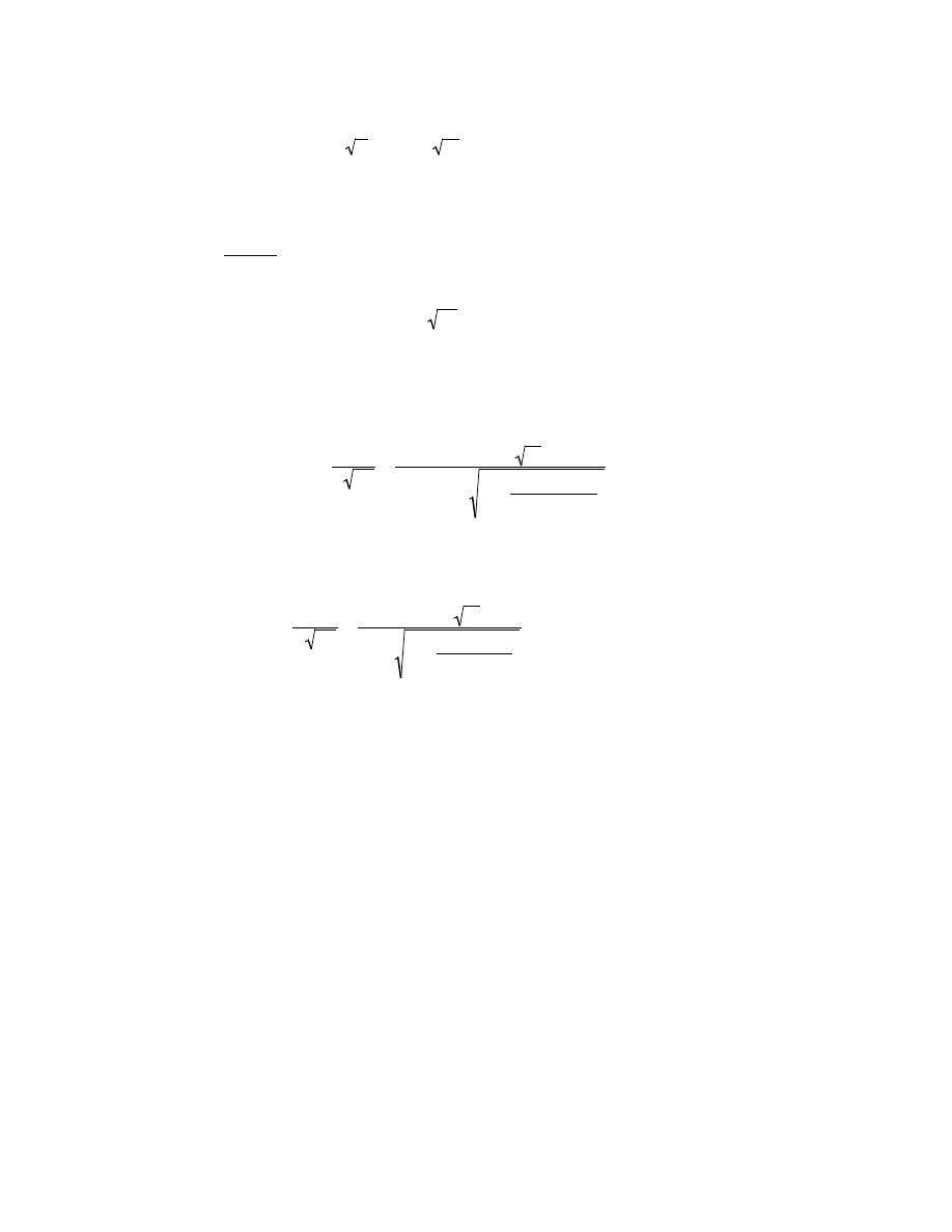
Excerpts from this work may be reproduced by instructors for distribution on a not-for-profit basis for testing or instructional purposes only to
students enrolled in courses for which the textbook has been adopted. Any other reproduction or translation of this work beyond that permitted
by Sections 107 or 108 of the 1976 United States Copyright Act without the permission of the copyright owner is unlawful.
8.7 Suppose that a wing component on an aircraft is fabricated from an aluminum alloy that has a plane
strain fracture toughness of
40 MPa m
(36.4 ksi in. ). It has been determined that fracture results at a stress of
365 MPa (53,000 psi) when the maximum internal crack length is 2.5 mm (0.10 in.). For this same component and
alloy, compute the stress level at which fracture will occur for a critical internal crack length of 4.0 mm (0.16 in.).
Solution
This problem asks us to determine the stress level at which an a wing component on an aircraft will
fracture for a given fracture toughness
(
40 MPa
m
)
and maximum internal crack length (4.0 mm), given that
fracture occurs for the same component using the same alloy at one stress level (365 MPa) and another internal
crack length (2.5 mm). It first becomes necessary to solve for the parameter Y for the conditions under which
fracture occurred using Equation 8.5. Therefore,
Y =
K
Ic
σ πa
=
40 MPa
m
(365 MPa)
(
π)
2.5
× 10
−3
m
2
= 1.75
Now we will solve for
σ
c
using Equation 8.6 as
σ
c
=
K
Ic
Y
πa
=
40 MPa m
(1.75)
(
π)
4
× 10
−3
m
2
= 288 MPa (41,500 psi)
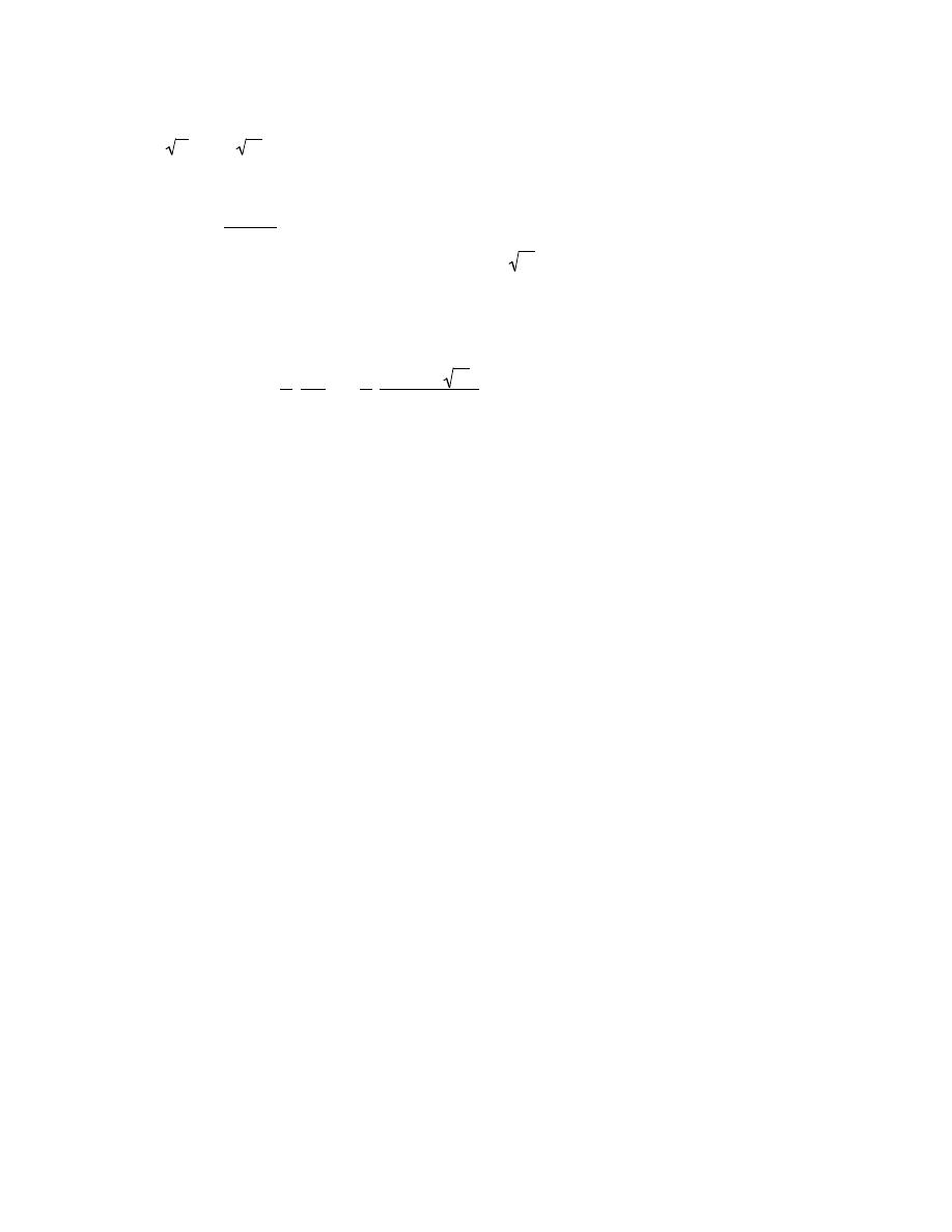
Excerpts from this work may be reproduced by instructors for distribution on a not-for-profit basis for testing or instructional purposes only to
students enrolled in courses for which the textbook has been adopted. Any other reproduction or translation of this work beyond that permitted
by Sections 107 or 108 of the 1976 United States Copyright Act without the permission of the copyright owner is unlawful.
8.8 A large plate is fabricated from a steel alloy that has a plane strain fracture toughness of
55 MPa m (50 ksi in. ). If, during service use, the plate is exposed to a tensile stress of 200 MPa (29,000 psi),
determine the minimum length of a surface crack that will lead to fracture. Assume a value of 1.0 for Y.
Solution
For this problem, we are given values of K
Ic
(
55 MPa
m
)
,
σ (200 MPa), and Y (1.0) for a large plate and
are asked to determine the minimum length of a surface crack that will lead to fracture. All we need do is to solve
for a
c
using Equation 8.7; therefore
a
c
=
1
π
K
Ic
Y
σ
2
=
1
π
55 MPa m
(1.0 )(200 MPa)
2
= 0.024 m = 24 mm (0.95 in.)
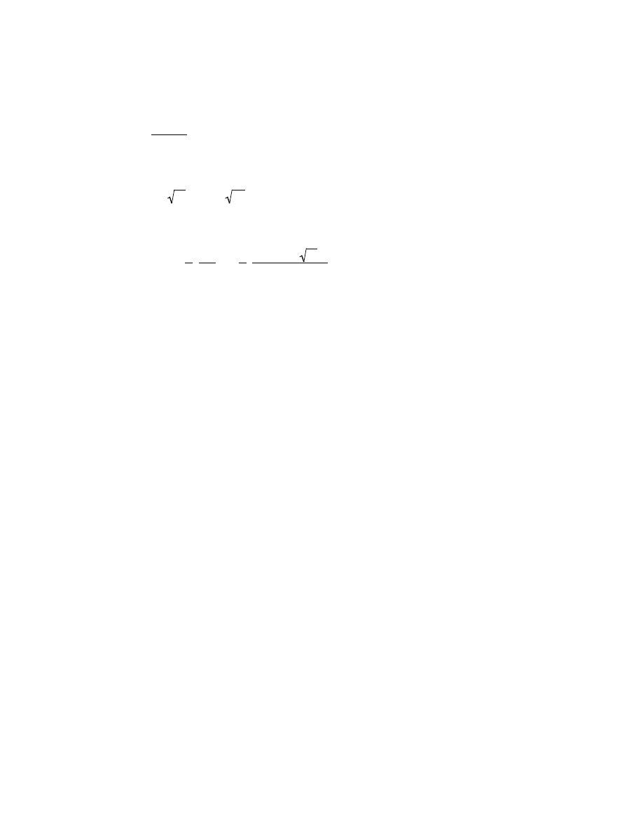
Excerpts from this work may be reproduced by instructors for distribution on a not-for-profit basis for testing or instructional purposes only to
students enrolled in courses for which the textbook has been adopted. Any other reproduction or translation of this work beyond that permitted
by Sections 107 or 108 of the 1976 United States Copyright Act without the permission of the copyright owner is unlawful.
8.9 Calculate the maximum internal crack length allowable for a 7075-T651 aluminum alloy (Table 8.1)
component that is loaded to a stress one half of its yield strength. Assume that the value of Y is 1.35.
Solution
This problem asks us to calculate the maximum internal crack length allowable for the 7075-T651
aluminum alloy in Table 8.1 given that it is loaded to a stress level equal to one-half of its yield strength. For this
alloy,
K
Ic
= 24 MPa m
(
22 ksi
in.
)
; also,
σ = σ
y
/2 = (495 MPa)/2 = 248 MPa (36,000 psi). Now solving for
2a
c
using Equation 8.7 yields
2a
c
=
2
π
K
Ic
Y
σ
2
=
2
π
24 MPa
m
(1.35)(248 MPa)
2
= 0.0033 m = 3.3 mm (0.13 in.)
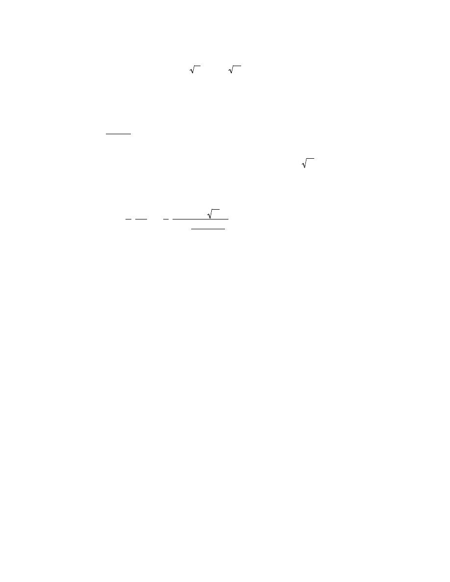
Excerpts from this work may be reproduced by instructors for distribution on a not-for-profit basis for testing or instructional purposes only to
students enrolled in courses for which the textbook has been adopted. Any other reproduction or translation of this work beyond that permitted
by Sections 107 or 108 of the 1976 United States Copyright Act without the permission of the copyright owner is unlawful.
8.10 A structural component in the form of a wide plate is to be fabricated from a steel alloy that has a
plane strain fracture toughness of
77.0 MPa m (70.1 ksi in. ) and a yield strength of 1400 MPa (205,000 psi).
The flaw size resolution limit of the flaw detection apparatus is 4.0 mm (0.16 in.). If the design stress is one half of
the yield strength and the value of Y is 1.0, determine whether or not a critical flaw for this plate is subject to
detection.
Solution
This problem asks that we determine whether or not a critical flaw in a wide plate is subject to detection
given the limit of the flaw detection apparatus (4.0 mm), the value of K
Ic
(
77 MPa
m
)
, the design stress (
σ
y
/2 in
which
σ
y
= 1400 MPa), and Y = 1.0. We first need to compute the value of a
c
using Equation 8.7; thus
a
c
=
1
π
K
Ic
Y
σ
2
=
1
π
77 MPa
m
(1.0 )
1400 MPa
2
2
= 0.0039 m = 3.9 mm (0.15 in.)
Therefore, the critical flaw is not subject to detection since this value of a
c
(3.9 mm) is less than the 4.0 mm
resolution limit.

Excerpts from this work may be reproduced by instructors for distribution on a not-for-profit basis for testing or instructional purposes only to
students enrolled in courses for which the textbook has been adopted. Any other reproduction or translation of this work beyond that permitted
by Sections 107 or 108 of the 1976 United States Copyright Act without the permission of the copyright owner is unlawful.
8.11 After consultation of other references, write a brief report on one or two nondestructive test
techniques that are used to detect and measure internal and/or surface flaws in metal alloys.
The student should do this problem on his/her own.
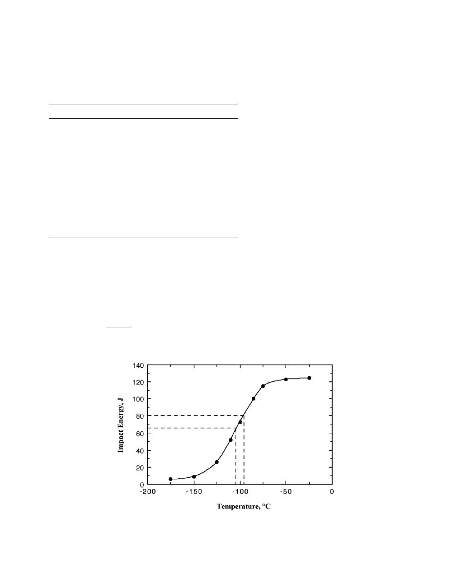
Excerpts from this work may be reproduced by instructors for distribution on a not-for-profit basis for testing or instructional purposes only to
students enrolled in courses for which the textbook has been adopted. Any other reproduction or translation of this work beyond that permitted
by Sections 107 or 108 of the 1976 United States Copyright Act without the permission of the copyright owner is unlawful.
Impact Fracture Testing
8.12 Following is tabulated data that were gathered from a series of Charpy impact tests on a ductile cast
iron.
Temperature (°C)
Impact Energy (J)
–25
124
–50
123
–75
115
–85
100
–100
73
–110
52
–125
26
–150
9
–175
6
(a) Plot the data as impact energy versus temperature.
(b) Determine a ductile-to-brittle transition temperature as that temperature corresponding to the average
of the maximum and minimum impact energies.
(c) Determine a ductile-to-brittle transition temperature as that temperature at which the impact energy is
80 J.
Solution
(a) The plot of impact energy versus temperature is shown below.

Excerpts from this work may be reproduced by instructors for distribution on a not-for-profit basis for testing or instructional purposes only to
students enrolled in courses for which the textbook has been adopted. Any other reproduction or translation of this work beyond that permitted
by Sections 107 or 108 of the 1976 United States Copyright Act without the permission of the copyright owner is unlawful.
(b) The average of the maximum and minimum impact energies from the data is
Average =
124 J
+ 6 J
2
= 65 J
As indicated on the plot by the one set of dashed lines, the ductile-to-brittle transition temperature according to this
criterion is about –105
°C.
(c) Also, as noted on the plot by the other set of dashed lines, the ductile-to-brittle transition temperature
for an impact energy of 80 J is about –95
°C.
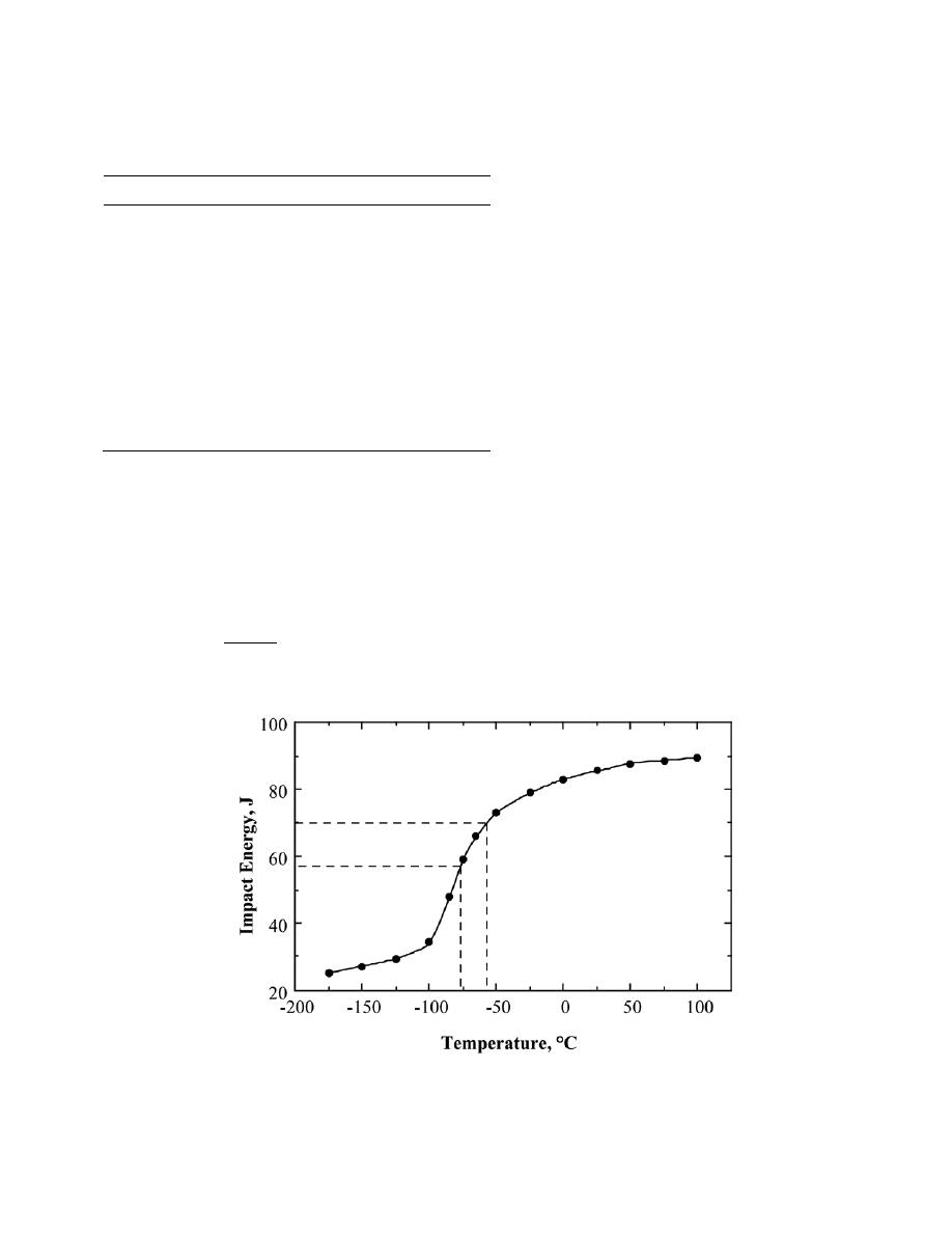
Excerpts from this work may be reproduced by instructors for distribution on a not-for-profit basis for testing or instructional purposes only to
students enrolled in courses for which the textbook has been adopted. Any other reproduction or translation of this work beyond that permitted
by Sections 107 or 108 of the 1976 United States Copyright Act without the permission of the copyright owner is unlawful.
8.13 Following is tabulated data that were gathered from a series of Charpy impact tests on a tempered
4140 steel alloy.
Temperature (°C)
Impact Energy (J)
100
89.3
75
88.6
50
87.6
25
85.4
0
82.9
–25
78.9
–50
73.1
–65
66.0
–75
59.3
–85
47.9
–100
34.3
–125
29.3
–150
27.1
–175
25.0
(a) Plot the data as impact energy versus temperature.
(b) Determine a ductile-to-brittle transition temperature as that temperature corresponding to the average
of the maximum and minimum impact energies.
(c) Determine a ductile-to-brittle transition temperature as that temperature at which the impact energy is
70 J.
Solution
The plot of impact energy versus temperature is shown below.

Excerpts from this work may be reproduced by instructors for distribution on a not-for-profit basis for testing or instructional purposes only to
students enrolled in courses for which the textbook has been adopted. Any other reproduction or translation of this work beyond that permitted
by Sections 107 or 108 of the 1976 United States Copyright Act without the permission of the copyright owner is unlawful.
(b) The average of the maximum and minimum impact energies from the data is
Average =
89.3 J
+ 25 J
2
= 57.2 J
As indicated on the plot by the one set of dashed lines, the ductile-to-brittle transition temperature according to this
criterion is about –75
°C.
(c) Also, as noted on the plot by the other set of dashed lines, the ductile-to-brittle transition temperature
for an impact energy of 70 J is about –55
°C.

Excerpts from this work may be reproduced by instructors for distribution on a not-for-profit basis for testing or instructional purposes only to
students enrolled in courses for which the textbook has been adopted. Any other reproduction or translation of this work beyond that permitted
by Sections 107 or 108 of the 1976 United States Copyright Act without the permission of the copyright owner is unlawful.
Cyclic Stresses (Fatigue)
The S-N Curve
8.14 A fatigue test was conducted in which the mean stress was 50 MPa (7250 psi) and the stress
amplitude was 225 MPa (32,625 psi).
(a) Compute the maximum and minimum stress levels.
(b) Compute the stress ratio.
(c) Compute the magnitude of the stress range.
Solution
(a) Given the values of
σ
m
(50 MPa) and
σ
a
(225 MPa) we are asked to compute
σ
max
and
σ
min
. From
Equation 8.14
σ
m
=
σ
max
+ σ
min
2
= 50 MPa
Or,
σ
max
+
σ
min
= 100 MPa
Furthermore, utilization of Equation 8.16 yields
σ
a
=
σ
max
− σ
min
2
= 225 MPa
Or,
σ
max
–
σ
min
= 450 MPa
Simultaneously solving these two expressions leads to
σ
max
= 275 MPa (40, 000 psi)
σ
min
=
−175 MPa (−25,500 psi)
(b) Using Equation 8.17 the stress ratio R is determined as follows:
R =
σ
min
σ
max
=
−175 MPa
275 MPa
=
− 0.64

Excerpts from this work may be reproduced by instructors for distribution on a not-for-profit basis for testing or instructional purposes only to
students enrolled in courses for which the textbook has been adopted. Any other reproduction or translation of this work beyond that permitted
by Sections 107 or 108 of the 1976 United States Copyright Act without the permission of the copyright owner is unlawful.
(c) The magnitude of the stress range
σ
r
is determined using Equation 8.15 as
σ
r
=
σ
max
− σ
min
= 275 MPa
− (−175 MPa) = 450 MPa (65,500 psi)
Excerpts from this work may be reproduced by instructors for distribution on a not-for-profit basis for testing or instructional purposes only to
students enrolled in courses for which the textbook has been adopted. Any other reproduction or translation of this work beyond that permitted
by Sections 107 or 108 of the 1976 United States Copyright Act without the permission of the copyright owner is unlawful.
8.15 A cylindrical 1045 steel bar (Figure 8.34) is subjected to repeated compression-tension stress cycling
along its axis. If the load amplitude is 22,000 N (4950 lb
f
), compute the minimum allowable bar diameter to ensure
that fatigue failure will not occur. Assume a factor of safety of 2.0.
Solution
From Figure 8.34, the fatigue limit stress amplitude for this alloy is 310 MPa (45,000 psi). Stress is
defined in Equation 6.1 as
σ =
F
A
0
. For a cylindrical bar
A
0
=
π
d
0
2
2
Substitution for A
0
into the Equation 6.1 leads to
σ =
F
A
0
=
F
π
d
0
2
2
=
4F
πd
0
2
We now solve for d
0
, taking stress as the fatigue limit divided by the factor of safety. Thus
d
0
=
4F
π
σ
N
=
(4)(22, 000 N)
(
π)
310
× 10
6
N / m
2
2
= 13.4 × 10
−3
m
= 13.4 mm (0.53 in.)

Excerpts from this work may be reproduced by instructors for distribution on a not-for-profit basis for testing or instructional purposes only to
students enrolled in courses for which the textbook has been adopted. Any other reproduction or translation of this work beyond that permitted
by Sections 107 or 108 of the 1976 United States Copyright Act without the permission of the copyright owner is unlawful.
8.16 An 8.0 mm (0.31 in.) diameter cylindrical rod fabricated from a red brass alloy (Figure 8.34) is
subjected to reversed tension-compression load cycling along its axis. If the maximum tensile and compressive
loads are +7500 N (1700 lb
f
) and -7500 N (-1700 lb
f
), respectively, determine its fatigue life. Assume that the
stress plotted in Figure 8.34 is stress amplitude.
Solution
We are asked to determine the fatigue life for a cylindrical red brass rod given its diameter (8.0 mm) and
the maximum tensile and compressive loads (+7500 N and -7500 N, respectively). The first thing that is necessary
is to calculate values of
σ
max
and
σ
min
using Equation 6.1. Thus
σ
max
=
F
max
A
0
=
F
max
π
d
0
2
2
=
7500 N
(
π)
8.0
× 10
−3
m
2
2
= 150
× 10
6
N/m
2
= 150 MPa (22, 500 psi)
σ
min
=
F
min
π
d
0
2
2
=
−7500 N
(
π)
8.0
× 10
−3
m
2
2
=
−150 × 10
6
N/m
2
=
−150 MPa (−22,500 psi)
Now it becomes necessary to compute the stress amplitude using Equation 8.16 as
σ
a
=
σ
max
− σ
min
2
=
150 MPa
− (−150 MPa)
2
= 150 MPa (22,500 psi)
From Figure 8.34, f for the red brass, the number of cycles to failure at this stress amplitude is about 1
× 10
5
cycles.

Excerpts from this work may be reproduced by instructors for distribution on a not-for-profit basis for testing or instructional purposes only to
students enrolled in courses for which the textbook has been adopted. Any other reproduction or translation of this work beyond that permitted
by Sections 107 or 108 of the 1976 United States Copyright Act without the permission of the copyright owner is unlawful.
8.17 A 12.5 mm (0.50 in.) diameter cylindrical rod fabricated from a 2014-T6 alloy (Figure 8.34) is
subjected to a repeated tension-compression load cycling along its axis. Compute the maximum and minimum
loads that will be applied to yield a fatigue life of 1.0
× 10
7
cycles. Assume that the stress plotted on the vertical
axis is stress amplitude, and data were taken for a mean stress of 50 MPa (7250 psi).
Solution
This problem asks that we compute the maximum and minimum loads to which a 12.5 mm (0.50 in.)
diameter 2014-T6 aluminum alloy specimen may be subjected in order to yield a fatigue life of 1.0
× 10
7
cycles;
Figure 8.34 is to be used assuming that data were taken for a mean stress of 50 MPa (7250 psi). Upon consultation
of Figure 8.34, a fatigue life of 1.0
× 10
7
cycles corresponds to a stress amplitude of 160 MPa (23,200 psi). Or,
from Equation 8.16
σ
max
− σ
min
= 2
σ
a
= (2)(160 MPa) = 320 MPa (46, 400 psi)
Since
σ
m
= 50 MPa, then from Equation 8.14
σ
max
+
σ
min
= 2
σ
m
= (2)(50 MPa) = 100 MPa (14, 500 psi)
Simultaneous solution of these two expressions for
σ
max
and
σ
min
yields
σ
max
= +210 MPa (+30,400 psi)
σ
min
= –110 MPa (–16,000 psi)
Now, inasmuch as
σ =
F
A
0
(Equation 6.1), and
A
0
=
π
d
0
2
2
then
F
max
=
σ
max
π d
0
2
4
=
(
210
× 10
6
N / m
2
)
(
π)
(
12.5
× 10
−3
m
)
2
4
= 25,800 N (6000 lb
f
)
F
min
=
σ
min
π d
0
2
4
=
(
−110 × 10
6
N / m
2
)
(
π)
(
12.5
× 10
−3
m
)
2
4
=
−13,500 N (−3140 lb
f
)
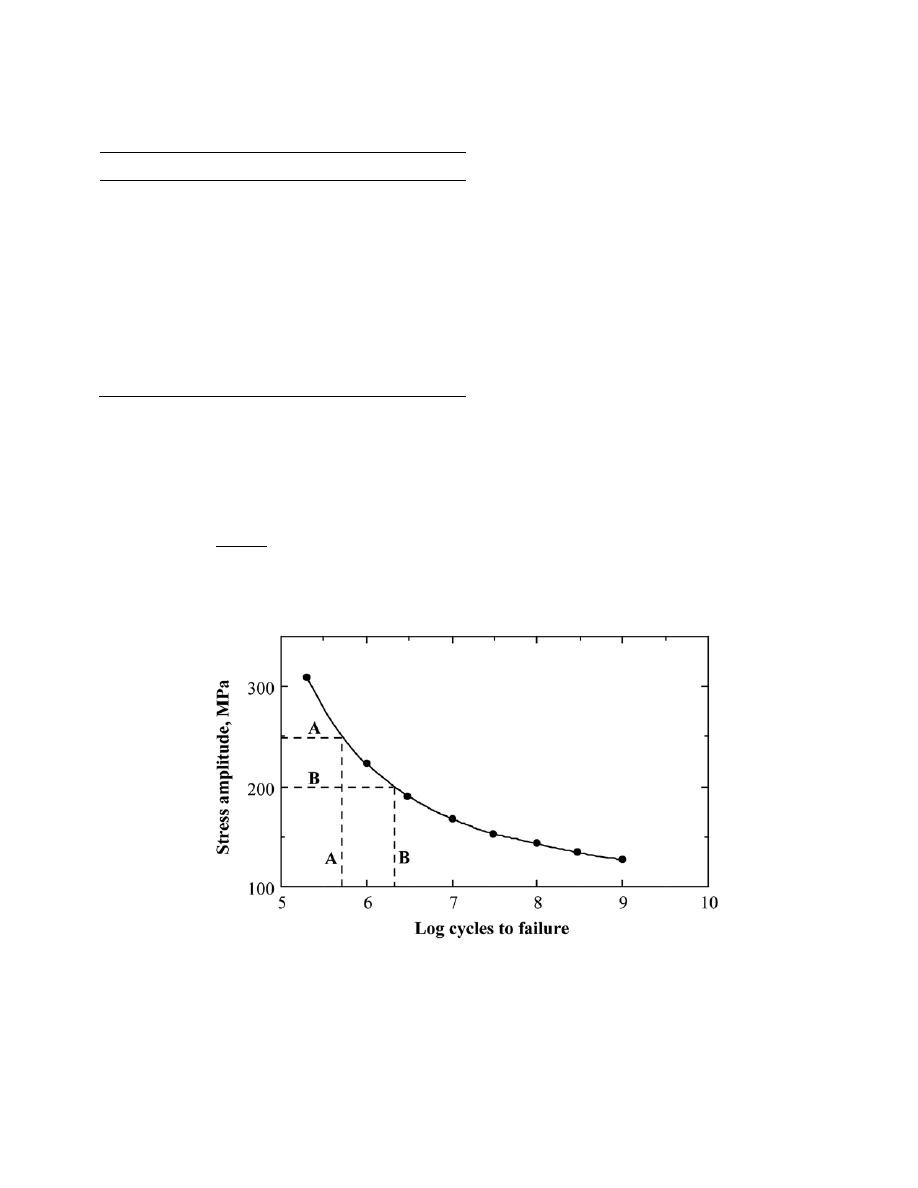
Excerpts from this work may be reproduced by instructors for distribution on a not-for-profit basis for testing or instructional purposes only to
students enrolled in courses for which the textbook has been adopted. Any other reproduction or translation of this work beyond that permitted
by Sections 107 or 108 of the 1976 United States Copyright Act without the permission of the copyright owner is unlawful.
8.18 The fatigue data for a brass alloy are given as follows:
Stress Amplitude (MPa)
Cycles to Failure
310
2 × 10
5
223
1 × 10
6
191
3 × 10
6
168
1 × 10
7
153
3 × 10
7
143
1 × 10
8
134
3 × 10
8
127
1 × 10
9
(a) Make an S–N plot (stress amplitude versus logarithm cycles to failure) using these data.
(b) Determine the fatigue strength at 5
× 10
5
cycles.
(c) Determine the fatigue life for 200 MPa.
Solution
(a) The fatigue data for this alloy are plotted below.
(b) As indicated by the “A” set of dashed lines on the plot, the fatigue strength at 5
× 10
5
cycles [log (5
×
10
5
) = 5.7] is about 250 MPa.

Excerpts from this work may be reproduced by instructors for distribution on a not-for-profit basis for testing or instructional purposes only to
students enrolled in courses for which the textbook has been adopted. Any other reproduction or translation of this work beyond that permitted
by Sections 107 or 108 of the 1976 United States Copyright Act without the permission of the copyright owner is unlawful.
(c) As noted by the “B” set of dashed lines, the fatigue life for 200 MPa is about 2
× 10
6
cycles (i.e., the
log of the lifetime is about 6.3).

Excerpts from this work may be reproduced by instructors for distribution on a not-for-profit basis for testing or instructional purposes only to
students enrolled in courses for which the textbook has been adopted. Any other reproduction or translation of this work beyond that permitted
by Sections 107 or 108 of the 1976 United States Copyright Act without the permission of the copyright owner is unlawful.
8.19 Suppose that the fatigue data for the brass alloy in Problem 8.18 were taken from torsional tests, and
that a shaft of this alloy is to be used for a coupling that is attached to an electric motor operating at 1500 rpm.
Give the maximum torsional stress amplitude possible for each of the following lifetimes of the coupling: (a) 1
year, (b) 1 month, (c) 1 day, and (d) 2 hours.
Solution
For each lifetime, first compute the number of cycles, and then read the corresponding fatigue strength
from the above plot.
(a) Fatigue lifetime = (1 yr)(365 days/yr)(24 h/day)(60 min/h)(1500 cycles/min) = 7.9
× 10
8
cycles. The
stress amplitude corresponding to this lifetime is about 130 MPa.
(b) Fatigue lifetime = (30 days)(24 h/day)(60 min/h)(1500 cycles/min) = 6.5
× 10
7
cycles. The stress
amplitude corresponding to this lifetime is about 145 MPa.
(c) Fatigue lifetime = (24 h)(60 min/h)(1500 cycles/min) = 2.2
× 10
6
cycles. The stress amplitude
corresponding to this lifetime is about 195 MPa.
(d) Fatigue lifetime = (2 h)(60 min/h)(1500 cycles/min) = 1.8
× 10
5
cycles. The stress amplitude
corresponding to this lifetime is about 315 MPa.
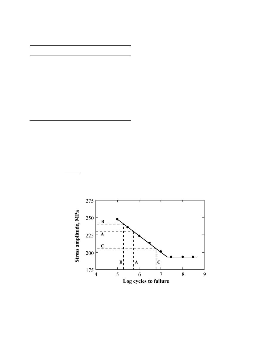
Excerpts from this work may be reproduced by instructors for distribution on a not-for-profit basis for testing or instructional purposes only to
students enrolled in courses for which the textbook has been adopted. Any other reproduction or translation of this work beyond that permitted
by Sections 107 or 108 of the 1976 United States Copyright Act without the permission of the copyright owner is unlawful.
8.20 The fatigue data for a ductile cast iron are given as follows:
Stress Amplitude
[MPa (ksi)]
Cycles to Failure
248 (36.0)
1 × 10
5
236 (34.2)
3 × 10
5
224 (32.5)
1 × 10
6
213 (30.9)
3 × 10
6
201 (29.1)
1 × 10
7
193 (28.0)
3 × 10
7
193 (28.0)
1 × 10
8
193 (28.0)
3 × 10
8
(a) Make an S–N plot (stress amplitude versus logarithm cycles to failure) using these data.
(b) What is the fatigue limit for this alloy?
(c) Determine fatigue lifetimes at stress amplitudes of 230 MPa (33,500 psi) and 175 MPa (25,000 psi).
(d) Estimate fatigue strengths at 2
× 10
5
and 6
× 10
6
cycles.
Solution
(a) The fatigue data for this alloy are plotted below.
(b) The fatigue limit is the stress level at which the curve becomes horizontal, which is 193 MPa (28,000
psi).

Excerpts from this work may be reproduced by instructors for distribution on a not-for-profit basis for testing or instructional purposes only to
students enrolled in courses for which the textbook has been adopted. Any other reproduction or translation of this work beyond that permitted
by Sections 107 or 108 of the 1976 United States Copyright Act without the permission of the copyright owner is unlawful.
(c) As noted by the “A” set of dashed lines, the fatigue lifetime at a stress amplitude of 230 MPa is about 5
× 10
5
cycles (log N = 5.7). From the plot, the fatigue lifetime at a stress amplitude of 230 MPa (33,500 psi) is about
50,000 cycles (log N = 4.7). At 175 MPa (25,000 psi) the fatigue lifetime is essentially an infinite number of cycles
since this stress amplitude is below the fatigue limit.
(d) As noted by the “B” set of dashed lines, the fatigue strength at 2
× 10
5
cycles (log N = 5.3) is about 240
MPa (35,000 psi); and according to the “C” set of dashed lines, the fatigue strength at 6
× 10
6
cycles (log N = 6.78)
is about 205 MPa (30,000 psi).

Excerpts from this work may be reproduced by instructors for distribution on a not-for-profit basis for testing or instructional purposes only to
students enrolled in courses for which the textbook has been adopted. Any other reproduction or translation of this work beyond that permitted
by Sections 107 or 108 of the 1976 United States Copyright Act without the permission of the copyright owner is unlawful.
8.21 Suppose that the fatigue data for the cast iron in Problem 8.20 were taken for bending-rotating tests,
and that a rod of this alloy is to be used for an automobile axle that rotates at an average rotational velocity of 750
revolutions per minute. Give maximum lifetimes of continuous driving that are allowable for the following stress
levels: (a) 250 MPa (36,250 psi), (b) 215 MPa (31,000 psi), (c) 200 MPa (29,000 psi), and (d) 150 MPa (21,750
psi).
Solution
For each stress level, first read the corresponding lifetime from the above plot, then convert it into the
number of cycles.
(a) For a stress level of 250 MPa (36,250 psi), the fatigue lifetime is approximately 90,000 cycles. This
translates into (9
× 10
4
cycles)(1 min/750 cycles) = 120 min.
(b) For a stress level of 215 MPa (31,000 psi), the fatigue lifetime is approximately 2
× 10
6
cycles. This
translates into (2
× 10
6
cycles)(1 min/750 cycles) = 2670 min = 44.4 h.
(c) For a stress level of 200 MPa (29,000 psi), the fatigue lifetime is approximately 1
× 10
7
cycles. This
translates into (1
× 10
7
cycles)(1 min/750 cycles) = 1.33
× 10
4
min = 222 h.
(d) For a stress level of 150 MPa (21,750 psi), the fatigue lifetime is essentially infinite since we are below
the fatigue limit [193 MPa (28,000 psi)].

Excerpts from this work may be reproduced by instructors for distribution on a not-for-profit basis for testing or instructional purposes only to
students enrolled in courses for which the textbook has been adopted. Any other reproduction or translation of this work beyond that permitted
by Sections 107 or 108 of the 1976 United States Copyright Act without the permission of the copyright owner is unlawful.
8.22 Three identical fatigue specimens (denoted A, B, and C) are fabricated from a nonferrous alloy. Each
is subjected to one of the maximum-minimum stress cycles listed below; the frequency is the same for all three tests.
Specimen
σ
max
(MPa)
σ
min
(MPa)
A
+450
–350
B
+400
–300
C
+340
–340
(a) Rank the fatigue lifetimes of these three specimens from the longest to the shortest.
(b) Now justify this ranking using a schematic S–N plot.
Solution
In order to solve this problem, it is necessary to compute both the mean stress and stress amplitude for each
specimen. Since from Equation 8.14, mean stresses are the specimens are determined as follows:
σ
m
=
σ
max
+ σ
min
2
σ
m
(A) =
450 MPa
+ (−350 MPa)
2
= 50 MPa
σ
m
( B) =
400 MPa
+ (−300 MPa)
2
= 50 MPa
σ
m
(C ) =
340 MPa
+ (−340 MPa)
2
= 0 MPa
Furthermore, using Equation 8.16, stress amplitudes are computed as
σ
a
=
σ
max
− σ
min
2
σ
a
(A) =
450 MPa
− (−350 MPa)
2
= 400 MPa
σ
a
( B) =
400 MPa
− (−300 MPa)
2
= 350 MPa
σ
a
(C ) =
340 MPa
− (−340 MPa)
2
= 340 MPa
On the basis of these results, the fatigue lifetime for specimen C will be greater than specimen B, which in turn will
be greater than specimen A. This conclusion is based upon the following S-N plot on which curves are plotted for
two
σ
m
values.
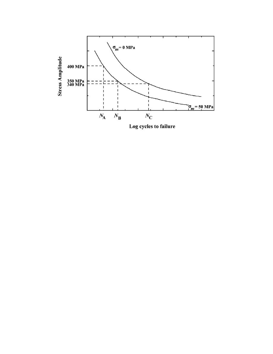
Excerpts from this work may be reproduced by instructors for distribution on a not-for-profit basis for testing or instructional purposes only to
students enrolled in courses for which the textbook has been adopted. Any other reproduction or translation of this work beyond that permitted
by Sections 107 or 108 of the 1976 United States Copyright Act without the permission of the copyright owner is unlawful.
8.23 Cite five factors that may lead to scatter in fatigue life data.
Solution
Five factors that lead to scatter in fatigue life data are (1) specimen fabrication and surface preparation, (2)
metallurgical variables, (3) specimen alignment in the test apparatus, (4) variation in mean stress, and (5) variation
in test cycle frequency.

Excerpts from this work may be reproduced by instructors for distribution on a not-for-profit basis for testing or instructional purposes only to
students enrolled in courses for which the textbook has been adopted. Any other reproduction or translation of this work beyond that permitted
by Sections 107 or 108 of the 1976 United States Copyright Act without the permission of the copyright owner is unlawful.
Crack Initiation and Propagation
Factors That Affect Fatigue Life
8.24 Briefly explain the difference between fatigue striations and beachmarks both in terms of (a) size and
(b) origin.
Solution
(a) With regard to size, beachmarks are normally of macroscopic dimensions and may be observed with
the naked eye; fatigue striations are of microscopic size and it is necessary to observe them using electron
microscopy.
(b) With regard to origin, beachmarks result from interruptions in the stress cycles; each fatigue striation
is corresponds to the advance of a fatigue crack during a single load cycle.

Excerpts from this work may be reproduced by instructors for distribution on a not-for-profit basis for testing or instructional purposes only to
students enrolled in courses for which the textbook has been adopted. Any other reproduction or translation of this work beyond that permitted
by Sections 107 or 108 of the 1976 United States Copyright Act without the permission of the copyright owner is unlawful.
8.25 List four measures that may be taken to increase the resistance to fatigue of a metal alloy.
Solution
Four measures that may be taken to increase the fatigue resistance of a metal alloy are:
(1) Polish the surface to remove stress amplification sites.
(2) Reduce the number of internal defects (pores, etc.) by means of altering processing and fabrication
techniques.
(3) Modify the design to eliminate notches and sudden contour changes.
(4) Harden the outer surface of the structure by case hardening (carburizing, nitriding) or shot peening.

Excerpts from this work may be reproduced by instructors for distribution on a not-for-profit basis for testing or instructional purposes only to
students enrolled in courses for which the textbook has been adopted. Any other reproduction or translation of this work beyond that permitted
by Sections 107 or 108 of the 1976 United States Copyright Act without the permission of the copyright owner is unlawful.
Generalized Creep Behavior
8.26 Give the approximate temperature at which creep deformation becomes an important consideration
for each of the following metals: nickel, copper, iron, tungsten, lead, and aluminum.
Solution
Creep becomes important at about 0.4T
m
, T
m
being the absolute melting temperature of the metal. (The
melting temperatures in degrees Celsius are found inside the front cover of the book.)
For Ni, 0.4T
m
= (0.4)(1455 + 273) = 691
K or 418
°C (785°F)
For Cu, 0.4T
m
= (0.4)(1085 + 273) = 543
K or 270
°C (518°F)
For Fe, 0.4T
m
= (0.4)(1538 + 273) = 725
K or 450
°C (845°F)
For W, 0.4T
m
= (0.4)(3410 + 273) = 1473
K or 1200
°C (2190°F)
For Pb, 0.4T
m
= (0.4)(327 + 273) = 240
K or
−33°C (−27°F)
For Al, 0.4T
m
= (0.4)(660 + 273) = 373
K or 100
°C (212°F)
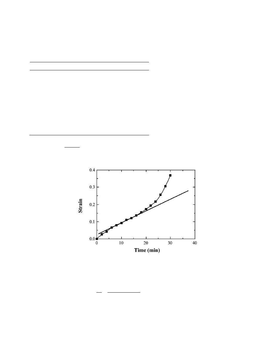
Excerpts from this work may be reproduced by instructors for distribution on a not-for-profit basis for testing or instructional purposes only to
students enrolled in courses for which the textbook has been adopted. Any other reproduction or translation of this work beyond that permitted
by Sections 107 or 108 of the 1976 United States Copyright Act without the permission of the copyright owner is unlawful.
8.27 The following creep data were taken on an aluminum alloy at 400
°C (750°F) and a constant stress of
25 MPa (3660 psi). Plot the data as strain versus time, then determine the steady-state or minimum creep rate.
Note: The initial and instantaneous strain is not included.
Time (min)
Strain
Time (min)
Strain
0
0.000
16
0.135
2
0.025
18
0.153
4
0.043
20
0.172
6
0.065
22
0.193
8
0.078
24
0.218
10
0.092
26
0.255
12
0.109
28
0.307
14
0.120
30
0.368
Solution
These creep data are plotted below
The steady-state creep rate (
∆ε/∆t) is the slope of the linear region (i.e., the straight line that has been
superimposed on the curve) as
∆ε
∆t
=
0.230
− 0.09
30 min
− 10 min
= 7.0
× 10
-3
min
-1

Excerpts from this work may be reproduced by instructors for distribution on a not-for-profit basis for testing or instructional purposes only to
students enrolled in courses for which the textbook has been adopted. Any other reproduction or translation of this work beyond that permitted
by Sections 107 or 108 of the 1976 United States Copyright Act without the permission of the copyright owner is unlawful.
Stress and Temperature Effects
8.28 A specimen 750 mm (30 in.) long of an S-590 alloy (Figure 8.31) is to be exposed to a tensile stress
of 80 MPa (11,600 psi) at 815
°C (1500°F). Determine its elongation after 5000 h. Assume that the total of both
instantaneous and primary creep elongations is 1.5 mm (0.06 in.).
Solution
From the 815
°C line in Figure 8.31, the steady state creep rate
Ý
ε
s
is about 5.5
× 10
-6
h
-1
at 80 MPa. The
steady state creep strain,
ε
s
, therefore, is just the product of
Ý
ε
s
and time as
ε
s
= Ý
ε
s
x (time)
=
(
5.5
× 10
−6
h
-1
)
(5,000 h) = 0.0275
Strain and elongation are related as in Equation 6.2; solving for the steady state elongation,
∆l
s
, leads to
∆l
s
= l
0
ε
s
= (750 mm)
(
0.0275
)
= 20.6 mm (0.81 in.)
Finally, the total elongation is just the sum of this
∆l
s
and the total of both instantaneous and primary creep
elongations [i.e., 1.5 mm (0.06 in.)]. Therefore, the total elongation is 20.6 mm + 1.5 mm = 22.1 mm (0.87 in.).

Excerpts from this work may be reproduced by instructors for distribution on a not-for-profit basis for testing or instructional purposes only to
students enrolled in courses for which the textbook has been adopted. Any other reproduction or translation of this work beyond that permitted
by Sections 107 or 108 of the 1976 United States Copyright Act without the permission of the copyright owner is unlawful.
8.29 For a cylindrical S-590 alloy specimen (Figure 8.31) originally 10 mm (0.40 in.) in diameter and 500
mm (20 in.) long, what tensile load is necessary to produce a total elongation of 145 mm (5.7 in.) after 2,000 h at
730
°C (1350°F)? Assume that the sum of instantaneous and primary creep elongations is 8.6 mm (0.34 in.).
Solution
It is first necessary to calculate the steady state creep rate so that we may utilize Figure 8.31 in order to
determine the tensile stress. The steady state elongation,
∆l
s
, is just the difference between the total elongation and
the sum of the instantaneous and primary creep elongations; that is,
∆l
s
= 145 mm
− 8.6 mm = 136.4 mm (5.36 in.)
Now the steady state creep rate,
Ý
ε
s
is just
ε
.
s
=
∆ε
∆ t
=
∆ l
s
l
0
∆ t
=
136.4 mm
500 mm
2, 000 h
= 1.36
× 10
-4
h
-1
Employing the 730
°C line in Figure 8.31, a steady state creep rate of 1.36 × 10
-4
h
-1
corresponds to a stress
σ of
about 200 MPa (or 29,000 psi) [since log (1.36
× 10
-4
) = -3.866]. From this we may compute the tensile load using
Equation 6.1 as
F =
σA
0
=
σπ
d
0
2
2
=
(
200
× 10
6
N/m
2
)
(
π)
10.0
× 10
−3
m
2
2
= 15, 700 N (3645 lb
f
)

Excerpts from this work may be reproduced by instructors for distribution on a not-for-profit basis for testing or instructional purposes only to
students enrolled in courses for which the textbook has been adopted. Any other reproduction or translation of this work beyond that permitted
by Sections 107 or 108 of the 1976 United States Copyright Act without the permission of the copyright owner is unlawful.
8.30 If a component fabricated from an S-590 alloy (Figure 8.30) is to be exposed to a tensile stress of
300 MPa (43,500 psi) at 650
°C (1200°F), estimate its rupture lifetime.
Solution
This problem asks us to calculate the rupture lifetime of a component fabricated from an S-590 alloy
exposed to a tensile stress of 300 MPa at 650
°C. All that we need do is read from the 650°C line in Figure 8.30 the
rupture lifetime at 300 MPa; this value is about 600 h.

Excerpts from this work may be reproduced by instructors for distribution on a not-for-profit basis for testing or instructional purposes only to
students enrolled in courses for which the textbook has been adopted. Any other reproduction or translation of this work beyond that permitted
by Sections 107 or 108 of the 1976 United States Copyright Act without the permission of the copyright owner is unlawful.
8.31 A cylindrical component constructed from an S-590 alloy (Figure 8.30) has a diameter of 12 mm
(0.50 in.). Determine the maximum load that may be applied for it to survive 500 h at 925
°C (1700°F).
Solution
We are asked in this problem to determine the maximum load that may be applied to a cylindrical S-590
alloy component that must survive 500 h at 925
°C. From Figure 8.30, the stress corresponding to 500 h is about 50
MPa (7,250 psi). Since stress is defined in Equation 6.1 as
σ = F/A
0
, and for a cylindrical specimen,
A
0
=
π
d
0
2
2
, then
F =
σA
0
=
σπ
d
0
2
2
=
(
50
× 10
6
N/m
2
)
(
π)
12
× 10
−3
m
2
2
= 5655 N (1424 lb
f
)

Excerpts from this work may be reproduced by instructors for distribution on a not-for-profit basis for testing or instructional purposes only to
students enrolled in courses for which the textbook has been adopted. Any other reproduction or translation of this work beyond that permitted
by Sections 107 or 108 of the 1976 United States Copyright Act without the permission of the copyright owner is unlawful.
8.32 From Equation 8.19, if the logarithm of
Ý
ε
s
is plotted versus the logarithm of σ, then a straight line
should result, the slope of which is the stress exponent n. Using Figure 8.31, determine the value of n for the S-590
alloy at 925°C, and for the initial (i.e., lower-temperature) straight line segments at each of 650°C, 730°C, and
815°C.
Solution
The slope of the line from a log
Ý
ε
s
versus log
σ plot yields the value of n in Equation 8.19; that is
n =
∆ log Ý
ε
s
∆ log σ
We are asked to determine the values of n for the creep data at the four temperatures in Figure 8.31 [i.e., at 925°C,
and for the initial (i.e., lower-temperature) straight line segments at each of 650°C, 730°C, and 815°C]. This is
accomplished by taking ratios of the differences between two log
Ý
ε
s
and log
σ values. (Note: Figure 8.31 plots log
σ versus log
Ý
ε
s
; therefore, values of n are equal to the reciprocals of the slopes of the straight-line segments.)
Thus for 650
°C
n =
∆ log Ý
ε
s
∆ log σ
=
log
(
10
−1
)
− log
(
10
−5
)
log (545 MPa)
− log (240 MPa)
= 11.2
While for 730
°C
n =
∆ log Ý
ε
s
∆ log σ
=
log 1
( )
− log
(
10
−6
)
log (430 MPa)
− log (125 MPa)
= 11.2
And at 815
°C
n =
∆ log Ý
ε
s
∆ log σ
=
log 1
( )
− log
(
10
−6
)
log (320 MPa)
− log (65 MPa)
= 8.7
And, finally at 925
°C
n =
∆ log Ý
ε
s
∆ log σ
=
log 10
2
( )
− log
(
10
−5
)
log (350 MPa)
− log (44 MPa)
= 7.8

Excerpts from this work may be reproduced by instructors for distribution on a not-for-profit basis for testing or instructional purposes only to
students enrolled in courses for which the textbook has been adopted. Any other reproduction or translation of this work beyond that permitted
by Sections 107 or 108 of the 1976 United States Copyright Act without the permission of the copyright owner is unlawful.
8.33 (a) Estimate the activation energy for creep (i.e., Q
c
in Equation 8.20) for the S-590 alloy having the
steady-state creep behavior shown in Figure 8.31. Use data taken at a stress level of 300 MPa (43,500 psi) and
temperatures of 650°C and 730°C . Assume that the stress exponent n is independent of temperature. (b) Estimate
Ý
ε
s
at 600°C (873 K) and 300 MPa.
Solution
(a) We are asked to estimate the activation energy for creep for the S-590 alloy having the steady-state
creep behavior shown in Figure 8.31, using data taken at
σ = 300 MPa and temperatures of 650°C and 730°C.
Since
σ is a constant, Equation 8.20 takes the form
Ý
ε
s
= K
2
σ
n
exp
−
Q
c
RT
= K
2
'
exp
−
Q
c
RT
where
K
2
'
is now a constant. (Note: the exponent n has about the same value at these two temperatures per
Problem 8.32.) Taking natural logarithms of the above expression
ln Ý
ε
s
= ln K
2
'
−
Q
c
RT
For the case in which we have creep data at two temperatures (denoted as T
1
and T
2
) and their corresponding
steady-state creep rates (
Ý
ε
s
1
and
Ý
ε
s
2
), it is possible to set up two simultaneous equations of the form as above, with
two unknowns, namely
K
2
'
and Q
c
. Solving for Q
c
yields
Q
c
=
−
R ln Ý
ε
s
1
− ln Ý
ε
s
2
1
T
1
−
1
T
2
Let us choose T
1
as 650
°C (923 K) and T
2
as 730
°C (1003 K); then from Figure 8.31, at σ = 300 MPa,
Ý
ε
s
1
= 8.9
×
10
-5
h
-1
and
Ý
ε
s
2
= 1.3
× 10
-2
h
-1
. Substitution of these values into the above equation leads to
Q
c
=
−
(8.31 J / mol - K) ln
(
8.9
× 10
−5
)
− ln
(
1.3
× 10
−2
)
[
]
1
923 K
−
1
1003 K
= 480,000 J/mol

Excerpts from this work may be reproduced by instructors for distribution on a not-for-profit basis for testing or instructional purposes only to
students enrolled in courses for which the textbook has been adopted. Any other reproduction or translation of this work beyond that permitted
by Sections 107 or 108 of the 1976 United States Copyright Act without the permission of the copyright owner is unlawful.
(b) We are now asked to estimate
Ý
ε
s
at 600
°C (873 K) and 300 MPa. It is first necessary to determine the
value of
K
2
'
, which is accomplished using the first expression above, the value of Q
c
, and one value each of
Ý
ε
s
and
T (say
Ý
ε
s
1
and T
1
). Thus,
K
2
'
= Ý
ε
s
1
exp
Q
c
RT
1
= 8.9
× 10
−5
h
−1
(
)
exp
480, 000 J / mol
(8.31 J / mol - K)(923 K)
= 1.34 × 10
23
h
-1
Now it is possible to calculate
Ý
ε
s
at 600
°C (873 K) and 300 MPa as follows:
Ý
ε
s
= K
2
'
exp
−
Q
c
RT
= 1.34
× 10
23
h
−1
(
)
exp
−
480, 000 J/mol
(8.31 J/mol - K)(873 K)
= 2.47
× 10
-6
h
-1

Excerpts from this work may be reproduced by instructors for distribution on a not-for-profit basis for testing or instructional purposes only to
students enrolled in courses for which the textbook has been adopted. Any other reproduction or translation of this work beyond that permitted
by Sections 107 or 108 of the 1976 United States Copyright Act without the permission of the copyright owner is unlawful.
8.34 Steady-state creep rate data are given below for nickel at 1000
°C (1273 K):
Ý
ε
s
(s
–1
)
σ [MPa (psi)]
10
–4
15 (2175)
10
–6
4.5 (650)
If it is known that the activation energy for creep is 272,000 J/mol, compute the steady-state creep rate at a
temperature of 850
°C (1123 K) and a stress level of 25 MPa (3625 psi).
Solution
Taking natural logarithms of both sides of Equation 8.20 yields
ln Ý
ε
s
= ln K
2
+ n ln σ −
Q
c
RT
With the given data there are two unknowns in this equation--namely K
2
and n. Using the data provided in the
problem statement we can set up two independent equations as follows:
ln 1
× 10
−4
s
−1
(
)
=
ln K
2
+ n ln (15 MPa)
−
272, 000 J / mol
(8.31 J/mol - K)(1273 K)
ln 1
× 10
−6
s
−1
(
)
=
ln K
2
+ n ln (4.5 MPa)
−
272, 000 J / mol
(8.31 J/mol - K)(1273 K)
Now, solving simultaneously for n and K
2
leads to n = 3.825 and K
2
= 466
s
-1
. Thus it is now possible to solve for
Ý
ε
s
at 25 MPa and 1123 K using Equation 8.20 as
Ý
ε
s
= K
2
σ
n
exp
−
Q
c
RT
= 466 s
−1
(
)
(25 MPa)
3.825
exp
−
272, 000 J/mol
(8.31 J/mol - K)(1123 K)
2.28
× 10
-5
s
-1

Excerpts from this work may be reproduced by instructors for distribution on a not-for-profit basis for testing or instructional purposes only to
students enrolled in courses for which the textbook has been adopted. Any other reproduction or translation of this work beyond that permitted
by Sections 107 or 108 of the 1976 United States Copyright Act without the permission of the copyright owner is unlawful.
8.35 Steady-state creep data taken for a stainless steel at a stress level of 70 MPa (10,000 psi) are given
as follows:
Ý
ε
s
(s
–1
)
T (K)
1.0 × 10
–5
977
2.5 × 10
–3
1089
If it is known that the value of the stress exponent n for this alloy is 7.0, compute the steady-state creep rate at 1250
K and a stress level of 50 MPa (7250 psi).
Solution
Taking natural logarithms of both sides of Equation 8.20 yields
ln Ý
ε
s
= ln K
2
+ n lnσ −
Q
c
RT
With the given data there are two unknowns in this equation--namely K
2
and Q
c
. Using the data provided in the
problem statement we can set up two independent equations as follows:
ln 1.0
× 10
−5
s
−1
(
)
=
ln K
2
+ (7.0) ln (70 MPa)
−
Q
c
(8.31 J/mol - K)(977 K)
ln 2.5
× 10
−3
s
−1
(
)
=
ln K
2
+ (7.0) ln (70 MPa)
−
Q
c
(8.31 J/mol - K)(1089 K)
Now, solving simultaneously for K
2
and Q
c
leads to K
2
= 2.55
× 10
5
s
-1
and Q
c
= 436,000 J/mol. Thus, it is now
possible to solve for
Ý
ε
s
at 50 MPa and 1250 K using Equation 8.20 as
Ý
ε
s
= K
2
σ
n
exp
−
Q
c
RT
= 2.55 × 10
5
s
−1
(
)
(50 MPa)
7.0
exp
−
436, 000 J/mol
(8.31 J/mol - K)(1250 K)
0.118 s
-1

Excerpts from this work may be reproduced by instructors for distribution on a not-for-profit basis for testing or instructional purposes only to
students enrolled in courses for which the textbook has been adopted. Any other reproduction or translation of this work beyond that permitted
by Sections 107 or 108 of the 1976 United States Copyright Act without the permission of the copyright owner is unlawful.
Alloys for High-Temperature Use
8.36 Cite three metallurgical/processing techniques that are employed to enhance the creep resistance of
metal alloys.
Solution
Three metallurgical/processing techniques that are employed to enhance the creep resistance of metal
alloys are (1) solid solution alloying, (2) dispersion strengthening by using an insoluble second phase, and (3)
increasing the grain size or producing a grain structure with a preferred orientation.

Excerpts from this work may be reproduced by instructors for distribution on a not-for-profit basis for testing or instructional purposes only to
students enrolled in courses for which the textbook has been adopted. Any other reproduction or translation of this work beyond that permitted
by Sections 107 or 108 of the 1976 United States Copyright Act without the permission of the copyright owner is unlawful.
DESIGN PROBLEMS
8.D1 Each student (or group of students) is to obtain an object/structure/component that has failed. It may
come from your home, an automobile repair shop, a machine shop, etc. Conduct an investigation to determine the
cause and type of failure (i.e., simple fracture, fatigue, creep). In addition, propose measures that can be taken to
prevent future incidents of this type of failure. Finally, submit a report that addresses the above issues.
Each student or group of students is to submit their own report on a failure analysis investigation that was
conducted.

Excerpts from this work may be reproduced by instructors for distribution on a not-for-profit basis for testing or instructional purposes only to
students enrolled in courses for which the textbook has been adopted. Any other reproduction or translation of this work beyond that permitted
by Sections 107 or 108 of the 1976 United States Copyright Act without the permission of the copyright owner is unlawful.
Principles of Fracture Mechanics
8.D2 (a) For the thin-walled spherical tank discussed in Design Example 8.1, on the basis of critical crack
size criterion [as addressed in part (a)], rank the following polymers from longest to shortest critical crack length:
nylon 6,6 (50% relative humidity), polycarbonate, poly(ethylene terephthalate), and poly(methyl methacrylate).
Comment on the magnitude range of the computed values used in the ranking relative to those tabulated for metal
alloys as provided in Table 8.3. For these computations, use data contained in Tables B.4 and B.5 in Appendix B.
(b) Now rank these same four polymers relative to maximum allowable pressure according to the leak-
before-break criterion, as described in the (b) portion of Design Example 8.1. As above, comment on these values
in relation to those for the metal alloys that are tabulated in Table 8.4.
Solution
(a) This portion of the problem calls for us to rank four polymers relative to critical crack length in the
wall of a spherical pressure vessel. In the development of Design Example 8.1, it was noted that critical crack
length is proportional to the square of the K
Ic
–
σ
y
ratio. Values of K
Ic
and
σ
y
as taken from Tables B.4 and B.5 are
tabulated below. (Note: when a range of
σ
y
or K
Ic
values is given, the average value is used.)
Material
K
Ic
(
MPa m
)
σ
y
(MPa)
Nylon 6,6
2.75
51.7
Polycarbonate
2.2
62.1
Poly(ethylene terephthlate)
5.0
59.3
Poly(methyl methacrylate)
1.2
63.5
On the basis of these values, the four polymers are ranked per the squares of the K
Ic
–
σ
y
ratios as follows:
Material
K
Ic
σ
y
2
(mm)
PET
7.11
Nylon 6,6
2.83
PC
1.26
PMMA
0.36

Excerpts from this work may be reproduced by instructors for distribution on a not-for-profit basis for testing or instructional purposes only to
students enrolled in courses for which the textbook has been adopted. Any other reproduction or translation of this work beyond that permitted
by Sections 107 or 108 of the 1976 United States Copyright Act without the permission of the copyright owner is unlawful.
These values are smaller than those for the metal alloys given in Table 8.3, which range from 0.93 to 43.1 mm.
(b) Relative to the leak-before-break criterion, the
K
Ic
2
-
σ
y
ratio is used. The four polymers are ranked
according to values of this ratio as follows:
Material
K
Ic
2
σ
y
(MPa - m)
PET
0.422
Nylon 6,6
0.146
PC
0.078
PMMA
0.023
These values are all smaller than those for the metal alloys given in Table 8.4, which values range from 1.2 to 11.2
MPa-m.

Excerpts from this work may be reproduced by instructors for distribution on a not-for-profit basis for testing or instructional purposes only to
students enrolled in courses for which the textbook has been adopted. Any other reproduction or translation of this work beyond that permitted
by Sections 107 or 108 of the 1976 United States Copyright Act without the permission of the copyright owner is unlawful.
Data Extrapolation Methods
8.D3 An S-590 alloy component (Figure 8.32) must have a creep rupture lifetime of at least 100 days at
500
°C (773 K). Compute the maximum allowable stress level.
Solution
This problem asks that we compute the maximum allowable stress level to give a rupture lifetime of 100
days for an S-590 iron component at 773 K. It is first necessary to compute the value of the Larson-Miller
parameter as follows:
T
(
20 + log t
r
)
= (773 K) 20 + log (100 days)(24 h/day)
[
]
{
}
= 18.1
× 10
3
From the curve in Figure 8.32, this value of the Larson-Miller parameter corresponds to a stress level of about 530
MPa (77,000 psi).

Excerpts from this work may be reproduced by instructors for distribution on a not-for-profit basis for testing or instructional purposes only to
students enrolled in courses for which the textbook has been adopted. Any other reproduction or translation of this work beyond that permitted
by Sections 107 or 108 of the 1976 United States Copyright Act without the permission of the copyright owner is unlawful.
8.D4 Consider an S-590 alloy component (Figure 8.32) that is subjected to a stress of 200 MPa (29,000
psi). At what temperature will the rupture lifetime be 500 h?
Solution
We are asked in this problem to calculate the temperature at which the rupture lifetime is 500 h when an S-
590 iron component is subjected to a stress of 200 MPa (29,000 psi). From the curve shown in Figure 8.32, at 200
MPa, the value of the Larson-Miller parameter is 22.5
× 10
3
(K-h). Thus,
22.5
× 10
3
(K - h) = T
(
20 + log t
r
)
= T 20 + log (500 h)
[
]
Or, solving for T yields T = 991 K (718
°C).

Excerpts from this work may be reproduced by instructors for distribution on a not-for-profit basis for testing or instructional purposes only to
students enrolled in courses for which the textbook has been adopted. Any other reproduction or translation of this work beyond that permitted
by Sections 107 or 108 of the 1976 United States Copyright Act without the permission of the copyright owner is unlawful.
8.D5 For an 18-8 Mo stainless steel (Figure 8.35), predict the time to rupture for a component that is
subjected to a stress of 80 MPa (11,600 psi) at 700
°C (973 K).
Solution
This problem asks that we determine, for an 18-8 Mo stainless steel, the time to rupture for a component
that is subjected to a stress of 80 MPa (11,600 psi) at 700
°C (973 K). From Figure 8.35, the value of the Larson-
Miller parameter at 80 MPa is about 23.5
× 10
3
, for T in K and t
r
in h. Therefore,
23.5
× 10
3
= T
(
20 + log t
r
)
= 973
(
20 + log t
r
)
And, solving for t
r
24.15 = 20 + log t
r
which leads to t
r
= 1.42
× 10
4
h = 1.6 yr.

Excerpts from this work may be reproduced by instructors for distribution on a not-for-profit basis for testing or instructional purposes only to
students enrolled in courses for which the textbook has been adopted. Any other reproduction or translation of this work beyond that permitted
by Sections 107 or 108 of the 1976 United States Copyright Act without the permission of the copyright owner is unlawful.
8.D6 Consider an 18-8 Mo stainless steel component (Figure 8.35) that is exposed to a temperature of
500
°C (773 K). What is the maximum allowable stress level for a rupture lifetime of 5 years? 20 years?
Solution
We are asked in this problem to calculate the stress levels at which the rupture lifetime will be 5 years and
20 years when an 18-8 Mo stainless steel component is subjected to a temperature of 500
°C (773 K). It first
becomes necessary to calculate the value of the Larson-Miller parameter for each time. The values of t
r
corresponding to 5 and 20 years are 4.38
× 10
4
h and 1.75
× 10
5
h, respectively. Hence, for a lifetime of 5 years
T
(
20 + log t
r
)
= 773 20 + log
(
4.38
× 10
4
)
[
]
= 19.05
× 10
3
And for t
r
= 20 years
T
(
20 + log t
r
)
= 773 20 + log
(
1.75
× 10
5
)
[
]
= 19.51
× 10
3
Using the curve shown in Figure 8.35, the stress values corresponding to the five- and twenty-year
lifetimes are approximately 260 MPa (37,500 psi) and 225 MPa (32,600 psi), respectively.

Excerpts from this work may be reproduced by instructors for distribution on a not-for-profit basis for testing or instructional purposes only to
students enrolled in courses for which the textbook has been adopted. Any other reproduction or translation of this work beyond that permitted
by Sections 107 or 108 of the 1976 United States Copyright Act without the permission of the copyright owner is unlawful.
CHAPTER 9
PHASE DIAGRAMS
PROBLEM SOLUTIONS
Solubility Limit
9.1 Consider the sugar–water phase diagram of Figure 9.1.
(a) How much sugar will dissolve in 1500 g water at 90
°C (194°F)?
(b) If the saturated liquid solution in part (a) is cooled to 20
°C (68°F), some of the sugar will precipitate
out as a solid. What will be the composition of the saturated liquid solution (in wt% sugar) at 20
°C?
(c) How much of the solid sugar will come out of solution upon cooling to 20
°C?
Solution
(a) We are asked to determine how much sugar will dissolve in 1000 g of water at 90
°C. From the
solubility limit curve in Figure 9.1, at 90
°C the maximum concentration of sugar in the syrup is about 77 wt%. It is
now possible to calculate the mass of sugar using Equation 4.3 as
C
sugar
(wt%) =
m
sugar
m
sugar
+ m
water
× 100
77 wt% =
m
sugar
m
sugar
+ 1500 g
× 100
Solving for m
sugar
yields m
sugar
= 5022 g
(b) Again using this same plot, at 20
°C the solubility limit (or the concentration of the saturated solution)
is about 64 wt% sugar.
(c) The mass of sugar in this saturated solution at 20
°C
(m'
sugar )
may also be calculated using Equation
4.3 as follows:
64 wt% =
m'
sugar
m'
sugar
+ 1500 g
× 100

Excerpts from this work may be reproduced by instructors for distribution on a not-for-profit basis for testing or instructional purposes only to
students enrolled in courses for which the textbook has been adopted. Any other reproduction or translation of this work beyond that permitted
by Sections 107 or 108 of the 1976 United States Copyright Act without the permission of the copyright owner is unlawful.
which yields a value for
m'
sugar
of 2667 g. Subtracting the latter from the former of these sugar concentrations
yields the amount of sugar that precipitated out of the solution upon cooling
m"
sugar
; that is
m"
sugar =
m
sugar −
mÕ
sugar =
5022 g
− 2667 g = 2355 g

Excerpts from this work may be reproduced by instructors for distribution on a not-for-profit basis for testing or instructional purposes only to
students enrolled in courses for which the textbook has been adopted. Any other reproduction or translation of this work beyond that permitted
by Sections 107 or 108 of the 1976 United States Copyright Act without the permission of the copyright owner is unlawful.
9.2 At 500
°C (930°F), what is the maximum solubility (a) of Cu in Ag? (b) Of Ag in Cu?
Solution
(a) From Figure 9.7, the maximum solubility of Cu in Ag at 500
°C corresponds to the position of the β–(α
+
β) phase boundary at this temperature, or to about 2 wt% Cu.
(b) From this same figure, the maximum solubility of Ag in Cu corresponds to the position of the
α–(α +
β) phase boundary at this temperature, or about 1.5 wt% Ag.

Excerpts from this work may be reproduced by instructors for distribution on a not-for-profit basis for testing or instructional purposes only to
students enrolled in courses for which the textbook has been adopted. Any other reproduction or translation of this work beyond that permitted
by Sections 107 or 108 of the 1976 United States Copyright Act without the permission of the copyright owner is unlawful.
Microstructure
9.3 Cite three variables that determine the microstructure of an alloy.
Solution
Three variables that determine the microstructure of an alloy are (1) the alloying elements present, (2) the
concentrations of these alloying elements, and (3) the heat treatment of the alloy.

Excerpts from this work may be reproduced by instructors for distribution on a not-for-profit basis for testing or instructional purposes only to
students enrolled in courses for which the textbook has been adopted. Any other reproduction or translation of this work beyond that permitted
by Sections 107 or 108 of the 1976 United States Copyright Act without the permission of the copyright owner is unlawful.
Phase Equilibria
9.4 What thermodynamic condition must be met for a state of equilibrium to exist?
Solution
In order for a system to exist in a state of equilibrium the free energy must be a minimum for some
specified combination of temperature, pressure, and composition.
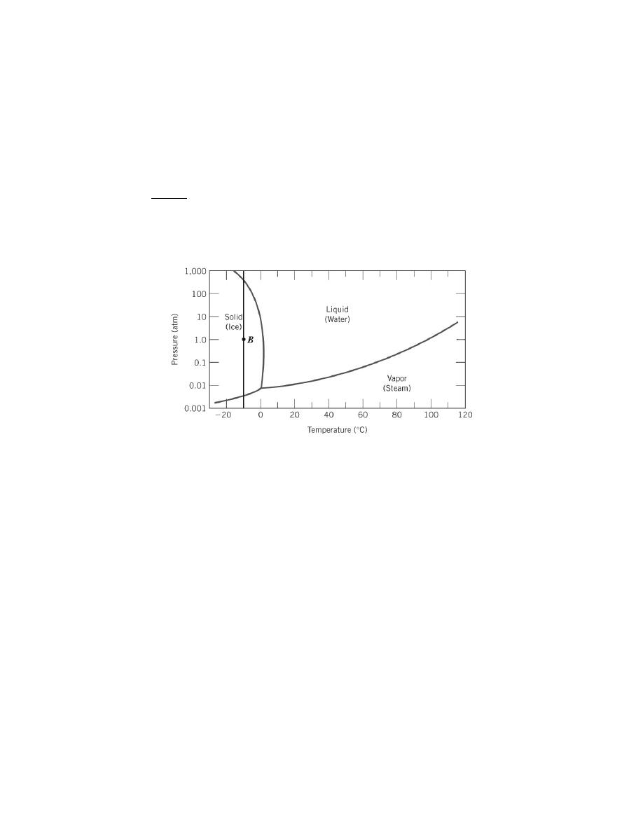
Excerpts from this work may be reproduced by instructors for distribution on a not-for-profit basis for testing or instructional purposes only to
students enrolled in courses for which the textbook has been adopted. Any other reproduction or translation of this work beyond that permitted
by Sections 107 or 108 of the 1976 United States Copyright Act without the permission of the copyright owner is unlawful.
One-Component (or Unary) Phase Diagrams
9.5 Consider a specimen of ice that is at 210
°C and 1 atm pressure. Using Figure 9.2, the pressure–
temperature phase diagram for H
2
O, determine the pressure to which the specimen must be raised or lowered to
cause it (a) to melt, and (b) to sublime.
Solution
The figure below shows the pressure-temperature phase diagram for H
2
O, Figure 10.2; a vertical line has
been constructed at -10
°C, and the location on this line at 1 atm pressure (point B) is also noted.
(a) Melting occurs, (by changing pressure) as, moving vertically (upward) at this temperature, we cross the
Ice-Liquid phase boundary. This occurs at approximately 570 atm; thus, the pressure of the specimen must be
raised from 1 to 570 atm.
(b) In order to determine the pressure at which sublimation occurs at this temperature, we move vertically
downward from 1 atm until we cross the Ice-Vapor phase boundary. This intersection occurs at approximately
0.0023 atm.
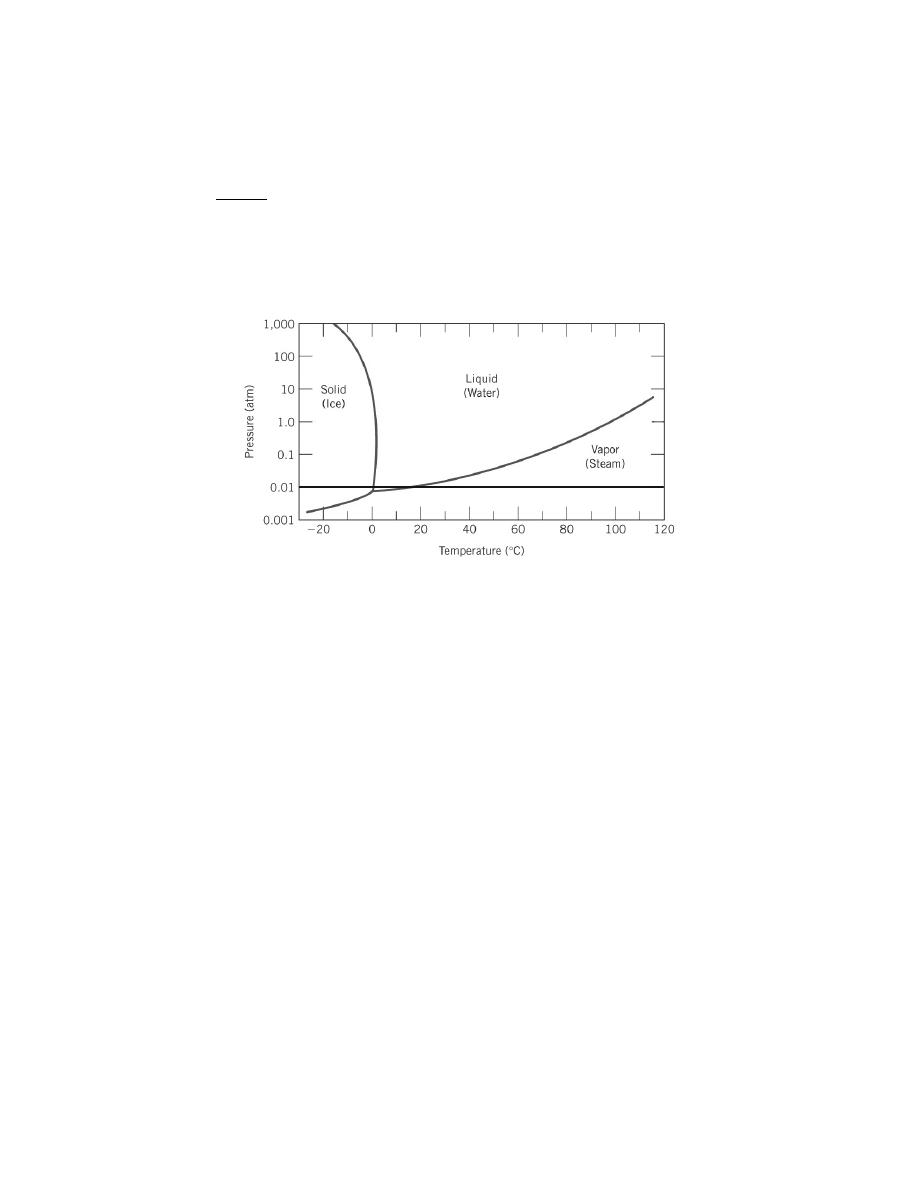
Excerpts from this work may be reproduced by instructors for distribution on a not-for-profit basis for testing or instructional purposes only to
students enrolled in courses for which the textbook has been adopted. Any other reproduction or translation of this work beyond that permitted
by Sections 107 or 108 of the 1976 United States Copyright Act without the permission of the copyright owner is unlawful.
9.6 At a pressure of 0.01 atm, determine (a) the melting temperature for ice, and (b) the boiling
temperature for water.
Solution
The melting temperature for ice and the boiling temperature for water at a pressure of 0.01 atm may be
determined from the pressure-temperature diagram for this system, Figure 10.2, which is shown below; a horizontal
line has been constructed across this diagram at a pressure of 0.01 atm.
The melting and boiling temperatures for ice at a pressure of 0.01 atm may be determined by moving horizontally
across the pressure-temperature diagram at this pressure. The temperature corresponding to the intersection of the
Ice-Liquid phase boundary is the melting temperature, which is approximately 1
°C. On the other hand, the boiling
temperature is at the intersection of the horizontal line with the Liquid-Vapor phase boundary--approximately 16
°C.
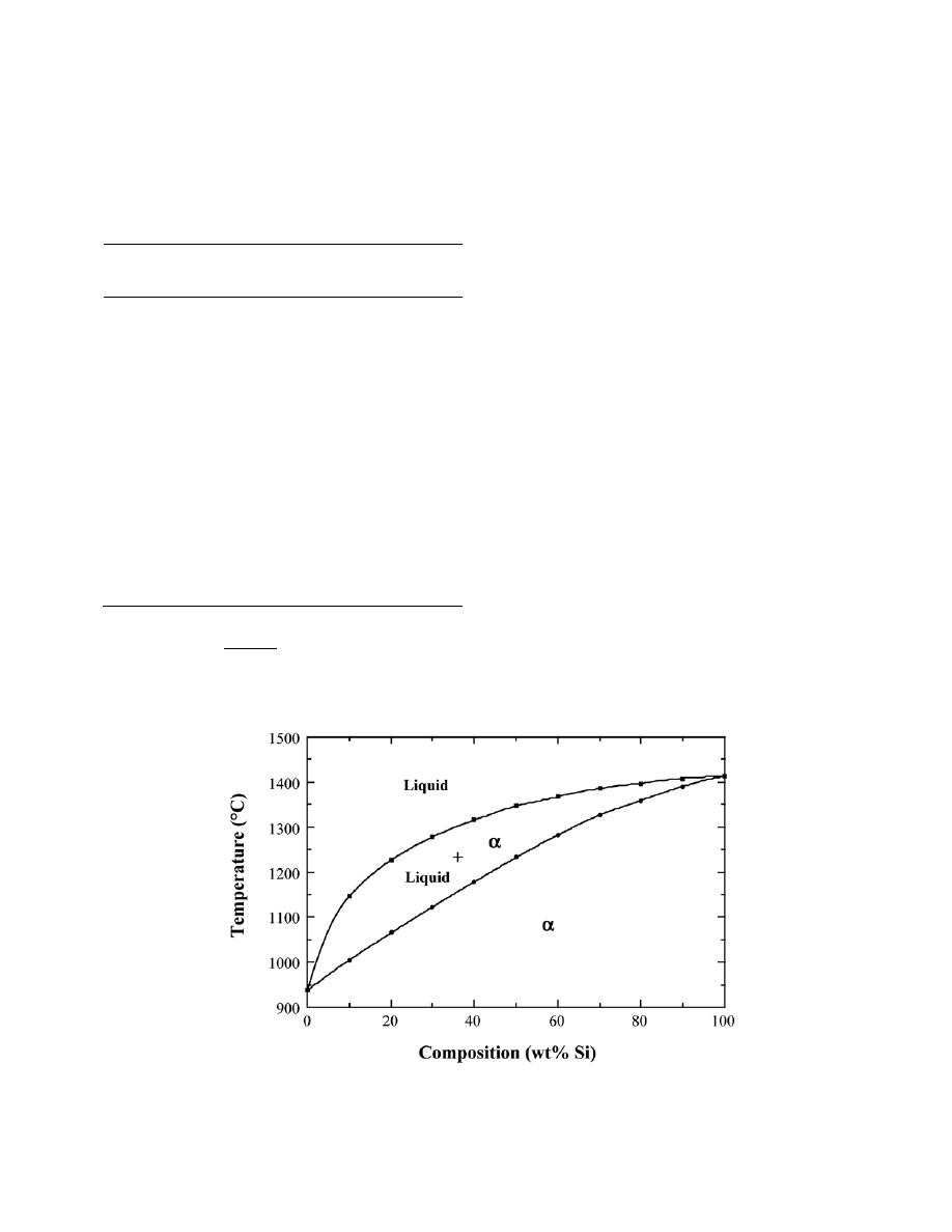
Excerpts from this work may be reproduced by instructors for distribution on a not-for-profit basis for testing or instructional purposes only to
students enrolled in courses for which the textbook has been adopted. Any other reproduction or translation of this work beyond that permitted
by Sections 107 or 108 of the 1976 United States Copyright Act without the permission of the copyright owner is unlawful.
Binary Isomorphous Systems
9.7 Given here are the solidus and liquidus temperatures for the germanium-silicon system. Construct the
phase diagram for this system and label each region.
Composition
(wt% Si)
Solidus
Temperature
(°C)
Liquidus
Temperature
(°C)
0
938
938
10
1005
1147
20
1065
1226
30
1123
1278
40
1178
1315
50
1232
1346
60
1282
1367
70
1326
1385
80
1359
1397
90
1390
1408
100
1414
1414
Solution
The germanium-silicon phase diagram is constructed below.
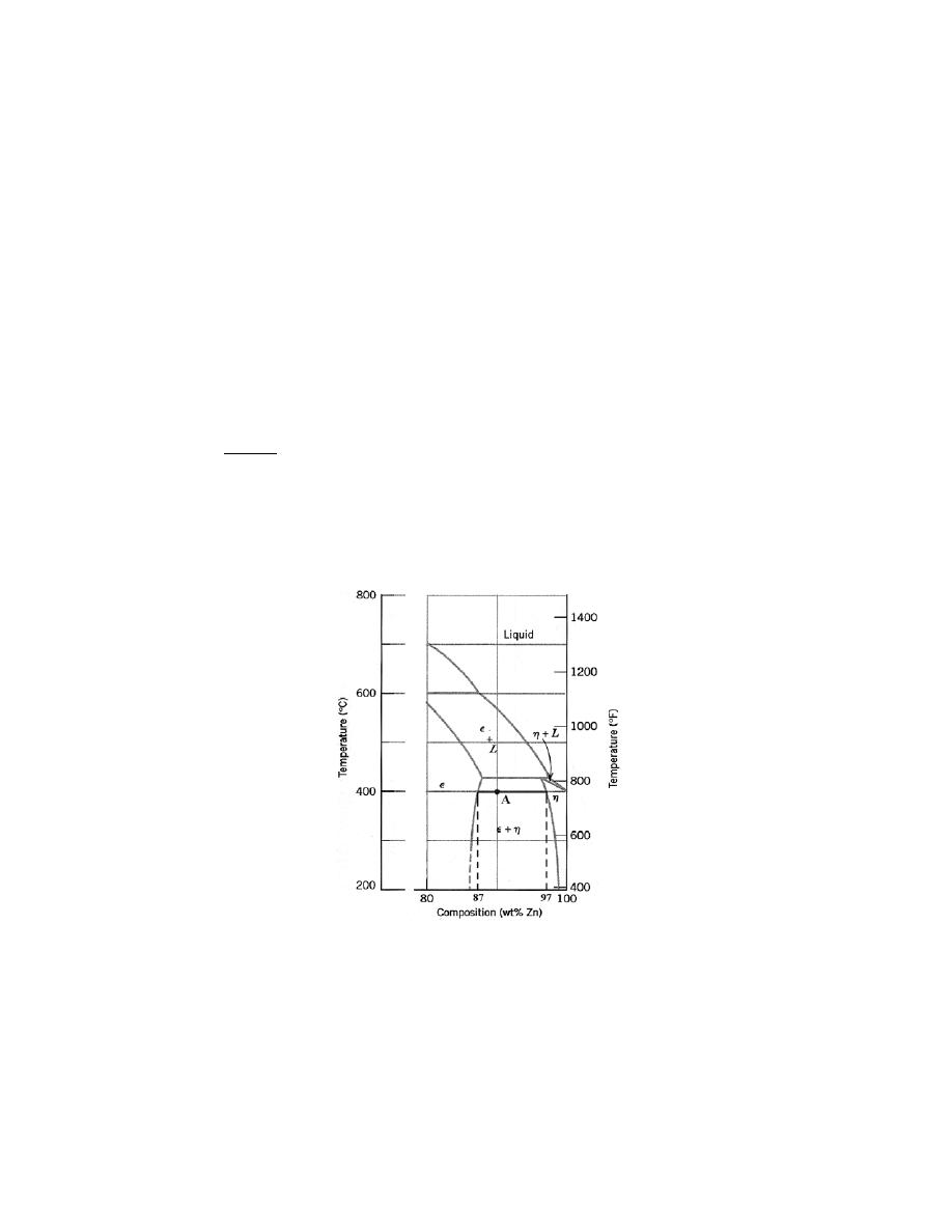
Excerpts from this work may be reproduced by instructors for distribution on a not-for-profit basis for testing or instructional purposes only to
students enrolled in courses for which the textbook has been adopted. Any other reproduction or translation of this work beyond that permitted
by Sections 107 or 108 of the 1976 United States Copyright Act without the permission of the copyright owner is unlawful.
Interpretation of Phase Diagrams
9.8 Cite the phases that are present and the phase compositions for the following alloys:
(a) 90 wt% Zn-10 wt% Cu at 400
°C (750°F)
(b) 75 wt% Sn-25 wt% Pb at 175
°C (345°F)
(c) 55 wt% Ag-45 wt% Cu at 900
°C (1650°F)
(d) 30 wt% Pb-70 wt% Mg at 425
°C (795°F)
(e) 2.12 kg Zn and 1.88 kg Cu at 500
°C (930°F)
(f) 37 lb
m
Pb and 6.5 lb
m
Mg at 400
°C (750°F)
(g) 8.2 mol Ni and 4.3 mol Cu at 1250
°C (2280°F)
(h) 4.5 mol Sn and 0.45 mol Pb at 200
°C (390°F)
Solution
This problem asks that we cite the phase or phases present for several alloys at specified temperatures.
(a) That portion of the Cu-Zn phase diagram (Figure 9.19) that pertains to this problem is shown below;
the point labeled “A” represents the 90 wt% Zn-10 wt% Cu composition at 400
°C.
As may be noted, point A lies within the
ε and η phase field. A tie line has been constructed at 400°C; its
intersection with the
ε−ε + η phase boundary is at 87 wt% Zn, which corresponds to the composition of the ε phase.
Similarly, the tie-line intersection with the
ε + η−η phase boundary occurs at 97 wt% Zn, which is the composition
of the
η phase. Thus, the phase compositions are as follows:
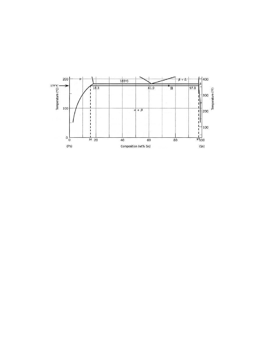
Excerpts from this work may be reproduced by instructors for distribution on a not-for-profit basis for testing or instructional purposes only to
students enrolled in courses for which the textbook has been adopted. Any other reproduction or translation of this work beyond that permitted
by Sections 107 or 108 of the 1976 United States Copyright Act without the permission of the copyright owner is unlawful.
C
ε
= 87 wt% Zn-13 wt% Cu
C
η
= 97 wt% Zn-3 wt% Cu
(b) That portion of the Pb-Sn phase diagram (Figure 9.8) that pertains to this problem is shown below; the
point labeled “B” represents the 75 wt% Sn-25 wt% Pb composition at 175
°C.
As may be noted, point B lies within the
α + β phase field. A tie line has been constructed at 175°C; its
intersection with the
α−α + β phase boundary is at 16 wt% Sn, which corresponds to the composition of the α
phase. Similarly, the tie-line intersection with the
α + β−β phase boundary occurs at 97 wt% Sn, which is the
composition of the
β phase. Thus, the phase compositions are as follows:
C
α
= 16 wt% Sn-84 wt% Pb
C
β
= 97 wt% Sn-3 wt% Pb
(c) The Ag-Cu phase diagram (Figure 9.7) is shown below; the point labeled “C” represents the 55 wt%
Ag-45 wt% Cu composition at 900
°C.
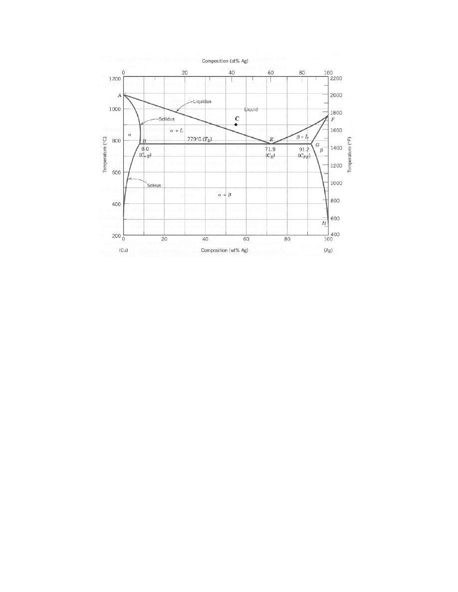
Excerpts from this work may be reproduced by instructors for distribution on a not-for-profit basis for testing or instructional purposes only to
students enrolled in courses for which the textbook has been adopted. Any other reproduction or translation of this work beyond that permitted
by Sections 107 or 108 of the 1976 United States Copyright Act without the permission of the copyright owner is unlawful.
As may be noted, point C lies within the Liquid phase field. Therefore, only the liquid phase is present; its
composition is 55 wt% Ag-45 wt% Cu.
(d) The Mg-Pb phase diagram (Figure 9.20) is shown below; the point labeled “D” represents the 30 wt%
Pb-70 wt% Mg composition at 425
°C.
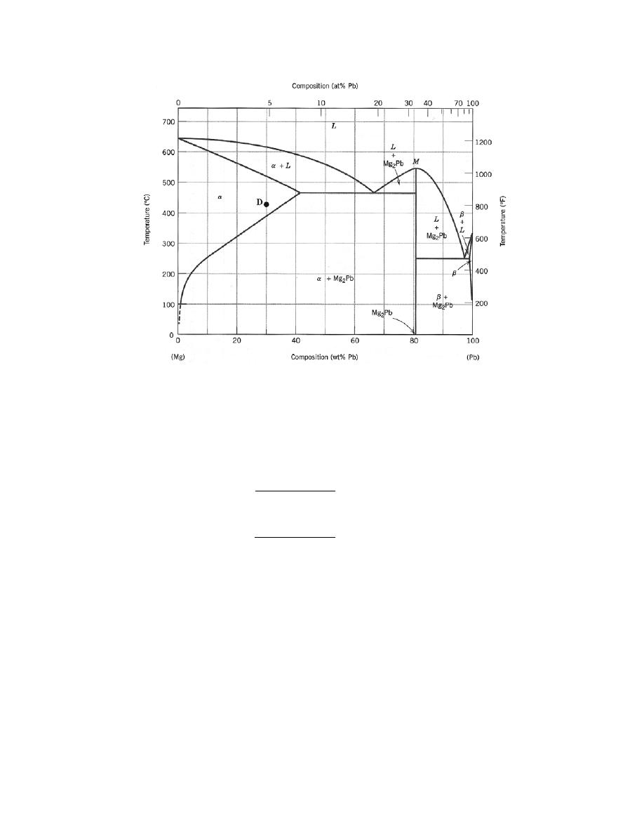
Excerpts from this work may be reproduced by instructors for distribution on a not-for-profit basis for testing or instructional purposes only to
students enrolled in courses for which the textbook has been adopted. Any other reproduction or translation of this work beyond that permitted
by Sections 107 or 108 of the 1976 United States Copyright Act without the permission of the copyright owner is unlawful.
As may be noted, point D lies within the
α phase field. Therefore, only the α phase is present; its composition is
30 wt% Pb-70 wt% Mg.
(e) For an alloy composed of 2.12 kg Zn and 1.88 kg Cu and at 500
°C, we must first determine the Zn and
Cu concentrations, as
C
Zn
=
2.12 kg
2.12 kg
+ 1.88 kg
× 100 = 53 wt%
C
Cu
=
1.88 kg
2.12 kg
+ 1.88 kg
× 100 = 47 wt%
That portion of the Cu-Zn phase diagram (Figure 9.19) that pertains to this problem is shown below; the point
labeled “E” represents the 53 wt% Zn-47 wt% Cu composition at 500
°C.
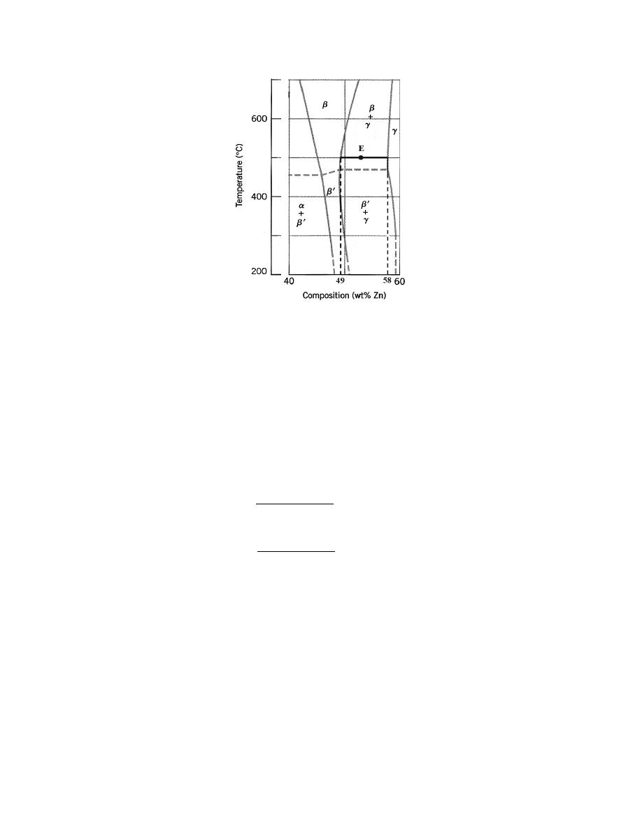
Excerpts from this work may be reproduced by instructors for distribution on a not-for-profit basis for testing or instructional purposes only to
students enrolled in courses for which the textbook has been adopted. Any other reproduction or translation of this work beyond that permitted
by Sections 107 or 108 of the 1976 United States Copyright Act without the permission of the copyright owner is unlawful.
As may be noted, point E lies within the
β + γ phase field. A tie line has been constructed at 500°C; its intersection
with the
β−β + γ phase boundary is at 49 wt% Zn, which corresponds to the composition of the β phase. Similarly,
the tie-line intersection with the
β + γ−γ phase boundary occurs at 58 wt% Zn, which is the composition of the
γ phase. Thus, the phase compositions are as follows:
C
β
= 49 wt% Zn-51 wt% Cu
C
γ
= 58 wt% Zn-42 wt% Cu
(f) For an alloy composed of 37 lb
m
Pb and 6.5 lb
m
Mg and at 400
°C, we must first determine the Pb and
Mg concentrations, as
C
Pb
=
37 lb
m
37 lb
m
+ 6.5 lb
m
× 100 = 85 wt%
C
Mg
=
6.5 lb
m
37 lb
m
+ 6.5 lb
m
× 100 = 15 wt%
That portion of the Mg-Pb phase diagram (Figure 9.20) that pertains to this problem is shown below; the point
labeled “F” represents the 85 wt% Pb-15 wt% Mg composition at 400
°C.
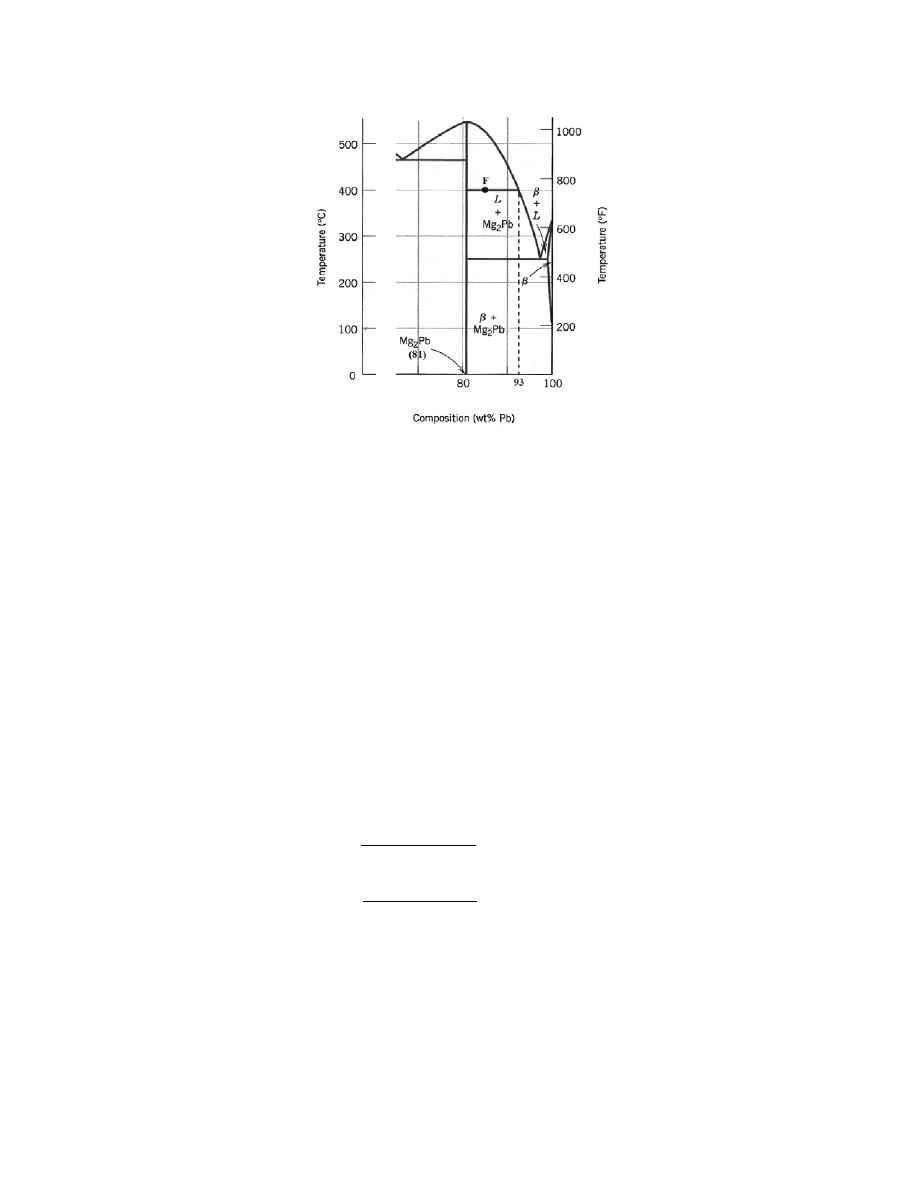
Excerpts from this work may be reproduced by instructors for distribution on a not-for-profit basis for testing or instructional purposes only to
students enrolled in courses for which the textbook has been adopted. Any other reproduction or translation of this work beyond that permitted
by Sections 107 or 108 of the 1976 United States Copyright Act without the permission of the copyright owner is unlawful.
As may be noted, point F lies within the L + Mg
2
Pb phase field. A tie line has been constructed at 400
°C; it
intersects the vertical line at 81 wt% Pb, which corresponds to the composition of Mg
2
Pb. Furthermore, the tie line
intersection with the L + Mg
2
Pb-L phase boundary is at 93 wt% Pb, which is the composition of the liquid phase.
Thus, the phase compositions are as follows:
C
Mg
2
Pb
= 81 wt% Pb-19 wt% Mg
C
L
= 93 wt% Pb-7 wt% Mg
(g) For an alloy composed of 8.2 mol Ni and 4.3 mol Cu and at 1250
°C, it is first necessary to determine
the Ni and Cu concentrations, which we will do in wt% as follows:
n
Ni
'
= n
m
Ni
A
Ni
= (8.2 mol)(58.69 g/mol) = 481.3 g
n
Cu
'
= n
m
Cu
A
Cu
= (4.3 mol)(63.55 g/mol) = 273.3 g
C
Ni
=
481.3 g
481.3 g + 273.3 g
× 100 = 63.8 wt%
C
Cu
=
273.3 g
481.3 g + 273.3 g
× 100 = 36.2 wt%
The Cu-Ni phase diagram (Figure 9.3a) is shown below; the point labeled “G” represents the 63.8 wt% Ni-36.2
wt% Cu composition at 1250
°C.
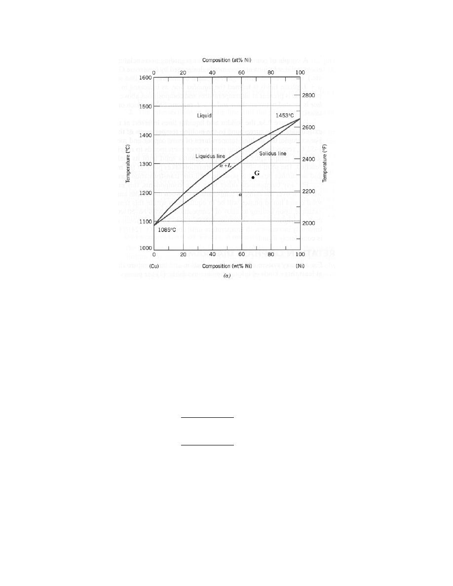
Excerpts from this work may be reproduced by instructors for distribution on a not-for-profit basis for testing or instructional purposes only to
students enrolled in courses for which the textbook has been adopted. Any other reproduction or translation of this work beyond that permitted
by Sections 107 or 108 of the 1976 United States Copyright Act without the permission of the copyright owner is unlawful.
As may be noted, point G lies within the
α phase field. Therefore, only the α phase is present; its composition is
63.8 wt% Ni-36.2 wt% Cu.
(h) For an alloy composed of 4.5 mol Sn and 0.45 mol Pb and at 200
°C, it is first necessary to determine
the Sn and Pb concentrations, which we will do in weight percent as follows:
n
Sn
’
= n
m
Sn
A
Sn
= (4.5 mol)(118.71 g/mol) = 534.2 g
n
Pb
'
= n
m
Pb
A
Pb
= (0.45 mol)(207.2 g/mol) = 93.2 g
C
Sn
=
534.2 g
534.2 g + 93.2 g
× 100 = 85.1 wt%
C
Pb
=
93.2 g
534.2 g + 93.2 g
× 100 = 14.9 wt%
That portion of the Pb-Sn phase diagram (Figure 9.8) that pertains to this problem is shown below; the point
labeled “H” represents the 85.1 wt% Sn-14.9 wt% Pb composition at 200
°C.
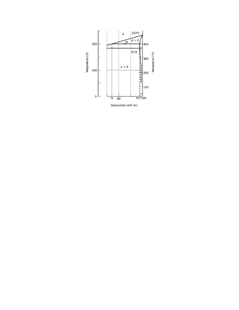
Excerpts from this work may be reproduced by instructors for distribution on a not-for-profit basis for testing or instructional purposes only to
students enrolled in courses for which the textbook has been adopted. Any other reproduction or translation of this work beyond that permitted
by Sections 107 or 108 of the 1976 United States Copyright Act without the permission of the copyright owner is unlawful.
As may be noted, point H lies within the
β + L phase field. A tie line has been constructed at 200°C; its intersection
with the L
−β + L phase boundary is at 74 wt% Sn, which corresponds to the composition of the L phase. Similarly,
the tie-line intersection with the
β + L−β phase boundary occurs at 97.5 wt% Sn, which is the composition of the
β phase. Thus, the phase compositions are as follows:
C
β
= 97.5 wt% Sn-2.5 wt% Pb
C
L
= 74 wt% Sn-26 wt% Pb

Excerpts from this work may be reproduced by instructors for distribution on a not-for-profit basis for testing or instructional purposes only to
students enrolled in courses for which the textbook has been adopted. Any other reproduction or translation of this work beyond that permitted
by Sections 107 or 108 of the 1976 United States Copyright Act without the permission of the copyright owner is unlawful.
9.9 Is it possible to have a copper–nickel alloy that, at equilibrium, consists of a liquid phase of
composition 20 wt% Ni–80 wt% Cu and also an
α phase of composition 37 wt% Ni–63 wt% Cu? If so, what will be
the approximate temperature of the alloy? If this is not possible, explain why.
Solution
It is not possible to have a Cu-Ni alloy, which at equilibrium, consists of a liquid phase of composition 20
wt% Ni-80 wt% Cu and an
α phase of composition 37 wt% Ni-63 wt% Cu. From Figure 9.3a, a single tie line does
not exist within the
α + L region that intersects the phase boundaries at the given compositions. At 20 wt% Ni, the
L-(
α + L) phase boundary is at about 1200°C, whereas at 37 wt% Ni the (L + α)-α phase boundary is at about
1230
°C.

Excerpts from this work may be reproduced by instructors for distribution on a not-for-profit basis for testing or instructional purposes only to
students enrolled in courses for which the textbook has been adopted. Any other reproduction or translation of this work beyond that permitted
by Sections 107 or 108 of the 1976 United States Copyright Act without the permission of the copyright owner is unlawful.
9.10 Is it possible to have a copper-zinc alloy that, at equilibrium, consists of an
ε phase of composition
80 wt% Zn-20 wt% Cu, and also a liquid phase of composition 95 wt% Zn-5 wt% Cu? If so, what will be the
approximate temperature of the alloy? If this is not possible, explain why.
Solution
It is not possible to have a Cu-Zn alloy, which at equilibrium consists of an
ε phase of composition 80 wt%
Zn-20 wt% Cu and also a liquid phase of composition 95 wt% Zn-5 wt% Cu. From Figure 9.19 a single tie line
does not exist within the
ε + L region which intersects the phase boundaries at the given compositions. At 80 wt%
Zn, the
ε-(ε + L) phase boundary is at about 575°C, whereas at 95 wt% Zn the (ε + L)-L phase boundary is at about
490
°C.
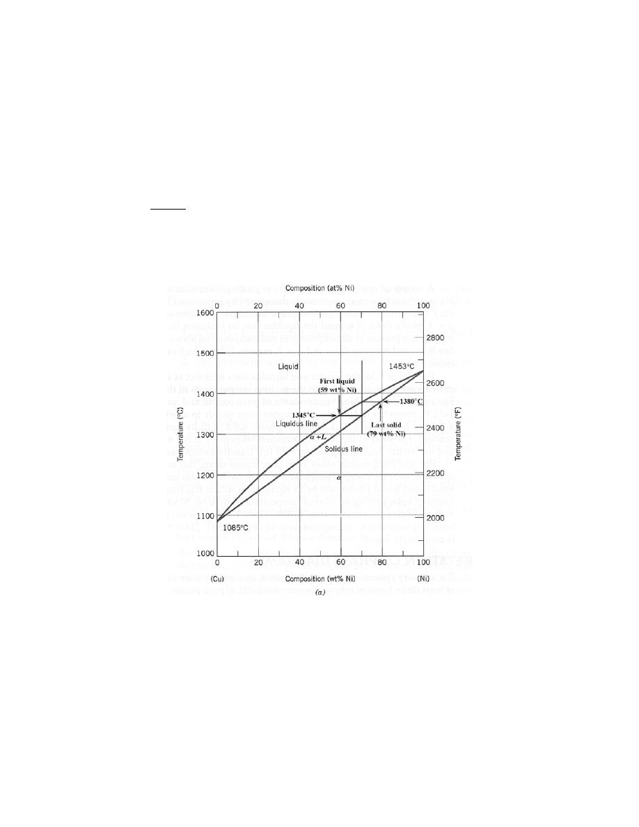
Excerpts from this work may be reproduced by instructors for distribution on a not-for-profit basis for testing or instructional purposes only to
students enrolled in courses for which the textbook has been adopted. Any other reproduction or translation of this work beyond that permitted
by Sections 107 or 108 of the 1976 United States Copyright Act without the permission of the copyright owner is unlawful.
9.11 A copper-nickel alloy of composition 70 wt% Ni-30 wt% Cu is slowly heated from a temperature of
1300
°C (2370°F).
(a) At what temperature does the first liquid phase form?
(b) What is the composition of this liquid phase?
(c) At what temperature does complete melting of the alloy occur?
(d) What is the composition of the last solid remaining prior to complete melting?
Solution
Shown below is the Cu-Ni phase diagram (Figure 9.3a) and a vertical line constructed at a composition of
70 wt% Ni-30 wt% Cu.
(a) Upon heating from 1300
°C, the first liquid phase forms at the temperature at which this vertical line
intersects the
α-(α + L) phase boundary--i.e., about 1345°C.
(b) The composition of this liquid phase corresponds to the intersection with the (
α + L)-L phase
boundary, of a tie line constructed across the
α + L phase region at 1345°C--i.e., 59 wt% Ni;
(c) Complete melting of the alloy occurs at the intersection of this same vertical line at 70 wt% Ni with the
(
α + L)-L phase boundary--i.e., about 1380°C;

Excerpts from this work may be reproduced by instructors for distribution on a not-for-profit basis for testing or instructional purposes only to
students enrolled in courses for which the textbook has been adopted. Any other reproduction or translation of this work beyond that permitted
by Sections 107 or 108 of the 1976 United States Copyright Act without the permission of the copyright owner is unlawful.
(d) The composition of the last solid remaining prior to complete melting corresponds to the intersection
with
α-(α + L) phase boundary, of the tie line constructed across the α + L phase region at 1380°C--i.e., about 79
wt% Ni.
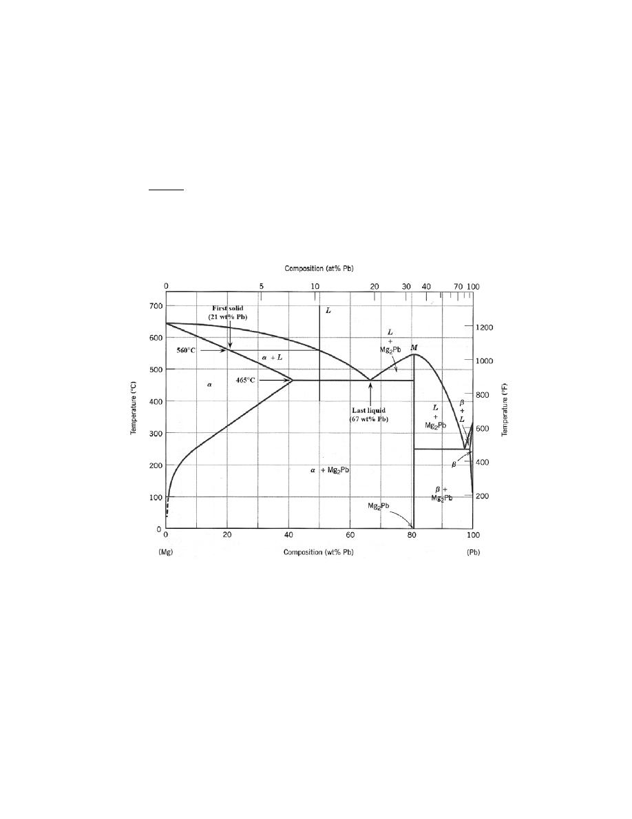
Excerpts from this work may be reproduced by instructors for distribution on a not-for-profit basis for testing or instructional purposes only to
students enrolled in courses for which the textbook has been adopted. Any other reproduction or translation of this work beyond that permitted
by Sections 107 or 108 of the 1976 United States Copyright Act without the permission of the copyright owner is unlawful.
9.12 A 50 wt% Pb-50 wt% Mg alloy is slowly cooled from 700
°C (1290°F) to 400°C (750°F).
(a) At what temperature does the first solid phase form?
(b) What is the composition of this solid phase?
(c) At what temperature does the liquid solidify?
(d) What is the composition of this last remaining liquid phase?
Solution
Shown below is the Mg-Pb phase diagram (Figure 9.20) and a vertical line constructed at a composition of
50 wt% Pb-50 wt% Mg.
(a) Upon cooling from 700
°C, the first solid phase forms at the temperature at which a vertical line at this
composition intersects the L-(
α + L) phase boundary--i.e., about 560°C;
(b) The composition of this solid phase corresponds to the intersection with the
α-(α + L) phase boundary,
of a tie line constructed across the
α + L phase region at 560°C--i.e., 21 wt% Pb-79 wt% Mg;
(c) Complete solidification of the alloy occurs at the intersection of this same vertical line at 50 wt% Pb
with the eutectic isotherm--i.e., about 465
°C;

Excerpts from this work may be reproduced by instructors for distribution on a not-for-profit basis for testing or instructional purposes only to
students enrolled in courses for which the textbook has been adopted. Any other reproduction or translation of this work beyond that permitted
by Sections 107 or 108 of the 1976 United States Copyright Act without the permission of the copyright owner is unlawful.
(d) The composition of the last liquid phase remaining prior to complete solidification corresponds to the
eutectic composition--i.e., about 67 wt% Pb-33 wt% Mg.
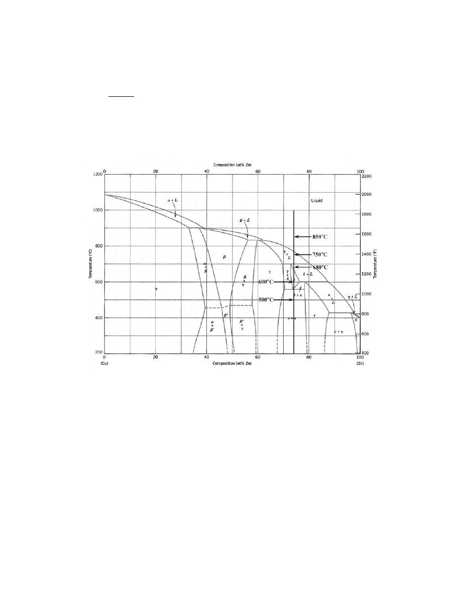
Excerpts from this work may be reproduced by instructors for distribution on a not-for-profit basis for testing or instructional purposes only to
students enrolled in courses for which the textbook has been adopted. Any other reproduction or translation of this work beyond that permitted
by Sections 107 or 108 of the 1976 United States Copyright Act without the permission of the copyright owner is unlawful.
9.13 For an alloy of composition 74 wt% Zn-26 wt% Cu, cite the phases present and their compositions at
the following temperatures: 850
°C, 750°C, 680°C, 600°C, and 500°C.
Solution
This problem asks us to determine the phases present and their concentrations at several temperatures, for
an alloy of composition 74 wt% Zn-26 wt% Cu. From Figure 9.19 (the Cu-Zn phase diagram), which is shown
below with a vertical line constructed at the specified composition:
At 850
°C, a liquid phase is present; C
L
= 74 wt% Zn-26 wt% Cu
At 750
°C, γ and liquid phases are present; C
γ
= 67 wt% Zn-33 wt% Cu; C
L
= 77 wt% Zn-23 wt% Cu
At 680
°C, δ and liquid phases are present; C
δ
= 73 wt% Zn-27 wt% Cu; C
L
= 82 wt% Zn-18 wt% Cu
At 600
°C, the δ phase is present; C
δ
= 74 wt% Zn-26 wt% Cu
At 500
°C, γ and ε phases are present; C
γ
= 69 wt% Zn-31 wt% Cu; C
ε
= 78 wt% Zn-22 wt% Cu
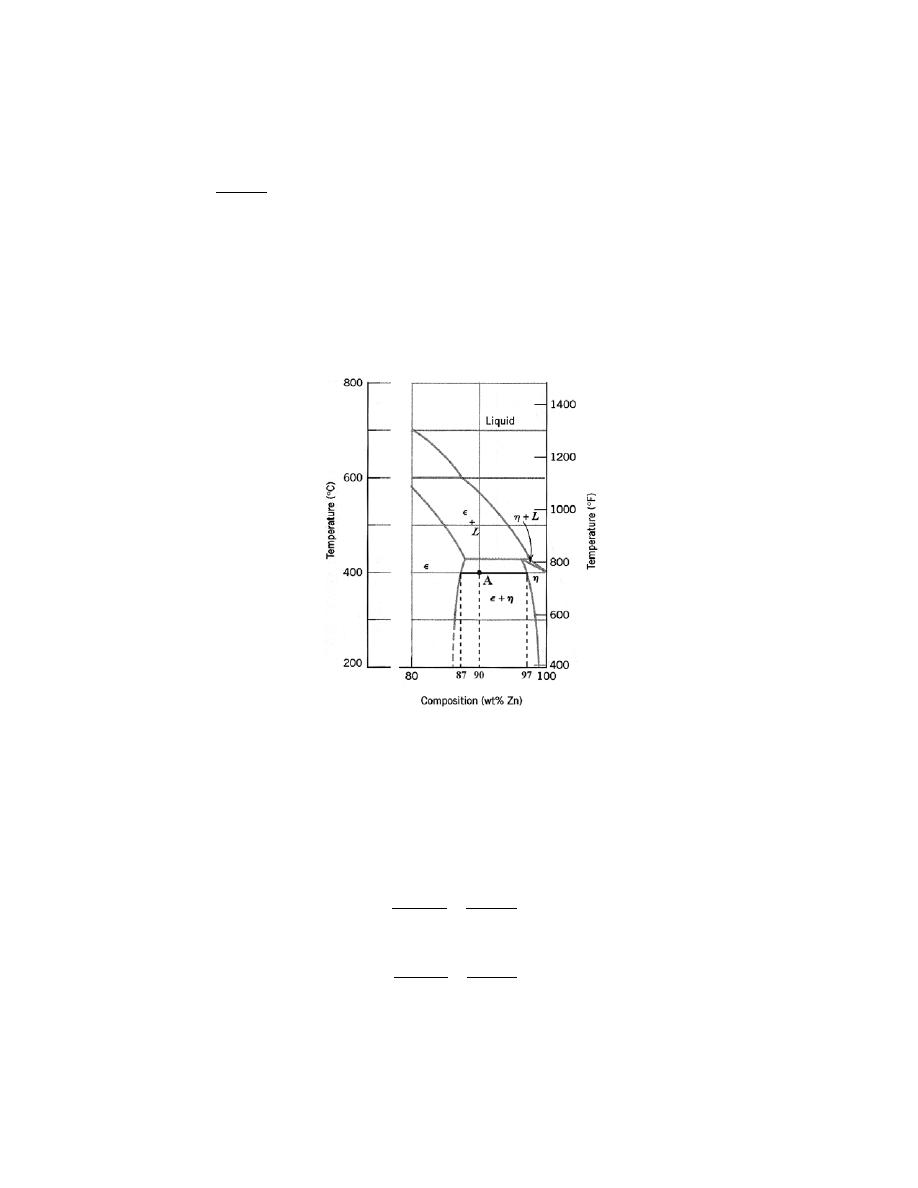
Excerpts from this work may be reproduced by instructors for distribution on a not-for-profit basis for testing or instructional purposes only to
students enrolled in courses for which the textbook has been adopted. Any other reproduction or translation of this work beyond that permitted
by Sections 107 or 108 of the 1976 United States Copyright Act without the permission of the copyright owner is unlawful.
9.14 Determine the relative amounts (in terms of mass fractions) of the phases for the alloys and
temperatures given in Problem 9.8.
Solution
This problem asks that we determine the phase mass fractions for the alloys and temperatures in Problem
9.8.
(a) From Problem 9.8a,
ε and η phases are present for a 90 wt% Zn-10 wt% Cu alloy at 400°C, as
represented in the portion of the Cu-Zn phase diagram shown below (at point A).
Furthermore, the compositions of the phases, as determined from the tie line are
C
ε
= 87 wt% Zn-13 wt% Cu
C
η
= 97 wt% Zn-3 wt% Cu
Inasmuch as the composition of the alloy C
0
= 90 wt% Zn, application of the appropriate lever rule expressions (for
compositions in weight percent zinc) leads to
W
ε
=
C
η
− C
0
C
η
− Cε
=
97
− 90
97
− 87
= 0.70
W
η
=
C
0
− C
ε
C
η
− Cε
=
90
− 87
97
− 87
= 0.30
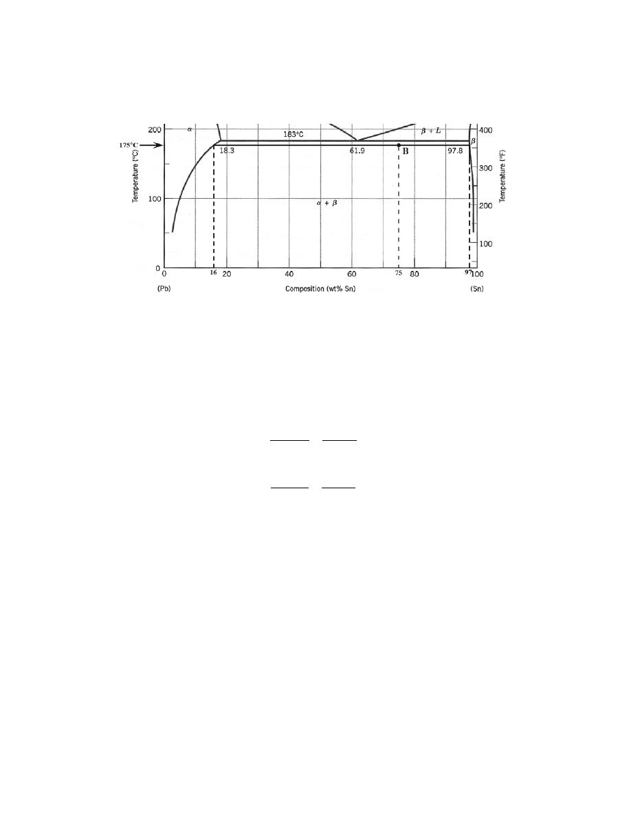
Excerpts from this work may be reproduced by instructors for distribution on a not-for-profit basis for testing or instructional purposes only to
students enrolled in courses for which the textbook has been adopted. Any other reproduction or translation of this work beyond that permitted
by Sections 107 or 108 of the 1976 United States Copyright Act without the permission of the copyright owner is unlawful.
(b) From Problem 9.8b,
α and β phases are present for a 75 wt% Sn-25 wt% Pb alloy at 175°C, as
represented in the portion of the Pb-Sn phase diagram shown below (at point B).
Furthermore, the compositions of the phases, as determined from the tie line are
C
α
= 16 wt% Sn-84 wt% Pb
C
β
= 97 wt% Sn-3 wt% Pb
Inasmuch as the composition of the alloy C
0
= 75 wt% Sn, application of the appropriate lever rule expressions (for
compositions in weight percent tin) leads to
W
α
=
C
β
− C
0
C
β
− Cα
=
97
− 75
97
− 16
= 0.27
W
β
=
C
0
− C
α
C
β
− C
α
=
75
− 16
97
− 16
= 0.73
(c) From Problem 9.8c, just the liquid phase is present for a 55 wt% Ag-45 wt% Cu alloy at 900
°C, as may
be noted in the Ag-Cu phase diagram shown below (at point C)—i.e., W
L
= 1.0
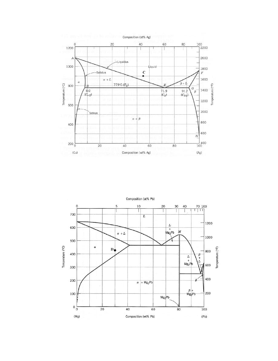
Excerpts from this work may be reproduced by instructors for distribution on a not-for-profit basis for testing or instructional purposes only to
students enrolled in courses for which the textbook has been adopted. Any other reproduction or translation of this work beyond that permitted
by Sections 107 or 108 of the 1976 United States Copyright Act without the permission of the copyright owner is unlawful.
(d) From Problem 9.8d, just the
α phase is present for a 30 wt% Pb-70 wt% Mg alloy at 425°C, as may be
noted in the Mg-Pb phase diagram shown below (at point D)—i.e., W
α
= 1.0
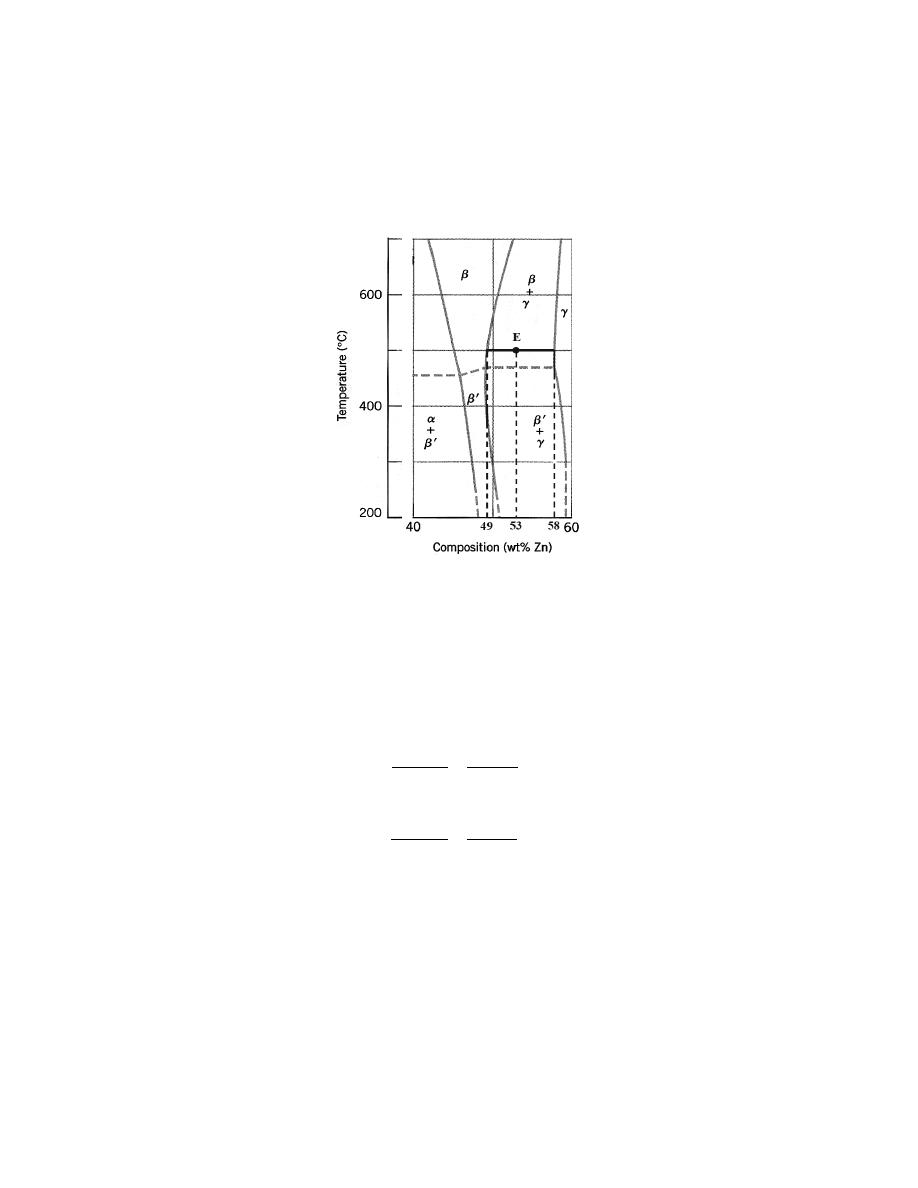
Excerpts from this work may be reproduced by instructors for distribution on a not-for-profit basis for testing or instructional purposes only to
students enrolled in courses for which the textbook has been adopted. Any other reproduction or translation of this work beyond that permitted
by Sections 107 or 108 of the 1976 United States Copyright Act without the permission of the copyright owner is unlawful.
(e) From Problem 9.8e,
β and γ phases are present for an alloy composed of 2.12 kg Zn and 1.88 kg Cu
(i.e., of composition 53 wt% Zn-47 wt% Cu) at 500
°C. This is represented in the portion of the Cu-Zn phase
diagram shown below (at point E).
Furthermore, the compositions of the phases, as determined from the tie line are
C
β
= 49 wt% Zn-51 wt% Cu
C
γ
= 58 wt% Zn-42 wt% Cu
Inasmuch as the composition of the alloy C
0
= 53 wt% Zn and application of the appropriate lever rule expressions
(for compositions in weight percent zinc) leads to
W
β
=
C
γ
− C
0
C
γ
− C
β
=
58
− 53
58
− 49
= 0.56
W
γ
=
C
0
− C
β
C
γ
− C
β
=
53
− 49
58
− 49
= 0.44
(f) From Problem 9.8f, L and Mg
2
Pb phases are present for an alloy composed of 37 lb
m
Pb and 6.5 lb
m
Mg (85 wt% Pb-15 wt% Mg) at 400
°C. This is represented in the portion of the Pb-Mg phase diagram shown
below (at point F).
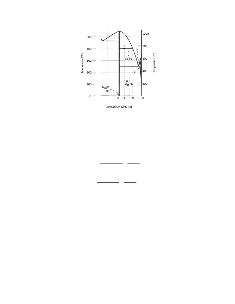
Excerpts from this work may be reproduced by instructors for distribution on a not-for-profit basis for testing or instructional purposes only to
students enrolled in courses for which the textbook has been adopted. Any other reproduction or translation of this work beyond that permitted
by Sections 107 or 108 of the 1976 United States Copyright Act without the permission of the copyright owner is unlawful.
Furthermore, the compositions of the phases, as determined from the tie line are
C
Mg
2
Pb
= 81 wt% Pb-19 wt% Mg
C
L
= 93 wt% Pb-7 wt% Mg
Inasmuch as the composition of the alloy C
0
= 85 wt% Pb and application of the appropriate lever rule expressions
(for compositions in weight percent lead) leads to
W
Mg
2
Pb
=
C
L
− C
0
C
L
− C
Mg
2
Pb
=
93
− 85
93
− 81
= 0.67
W
L
=
C
0
− C
Mg
2
Pb
C
L
− C
Mg
2
Pb
=
85
− 81
93
− 81
= 0.33
(g) From Problem 9.8g, just the
α phase is present (i.e., W
α
= 1.0) for an alloy composed of 8.2 mol Ni
and 4.3 mol Cu (i.e., 63.8 wt% Ni-36.2 wt% Cu) at 1250
°C; such may be noted (as point G) in the Cu-Ni phase
diagram shown below.
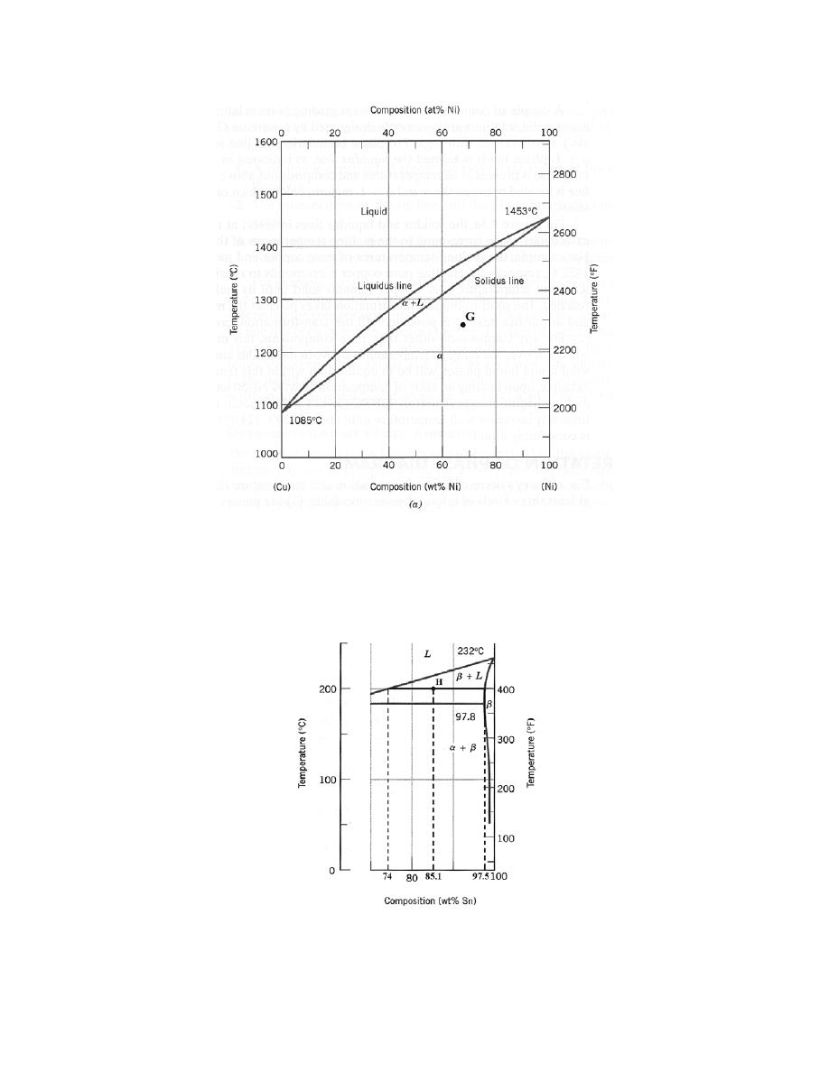
Excerpts from this work may be reproduced by instructors for distribution on a not-for-profit basis for testing or instructional purposes only to
students enrolled in courses for which the textbook has been adopted. Any other reproduction or translation of this work beyond that permitted
by Sections 107 or 108 of the 1976 United States Copyright Act without the permission of the copyright owner is unlawful.
(h) From Problem 9.8h,
β and L phases are present for an alloy composed of 4.5 mol Sn and 0.45 mol Pb
(85.1 wt% Sn-14.9 wt% Pb ) and at 200
°C. This is represented in the portion of the Pb-Sn phase diagram shown
below (at point H).
Furthermore, the compositions of the phases, as determined from the tie line are

Excerpts from this work may be reproduced by instructors for distribution on a not-for-profit basis for testing or instructional purposes only to
students enrolled in courses for which the textbook has been adopted. Any other reproduction or translation of this work beyond that permitted
by Sections 107 or 108 of the 1976 United States Copyright Act without the permission of the copyright owner is unlawful.
C
β
= 97.5 wt% Sn-2.5 wt% Pb
C
L
= 74 wt% Sn-26 wt% Pb
Inasmuch as the composition of the alloy C
0
= 85.1 wt% Sn, application of the appropriate lever rule expressions
(for compositions in weight percent lead) leads to
W
β
=
C
0
− C
L
C
β
− C
L
=
85.1
− 74
97.5
− 74
= 0.47
W
L
=
C
β
− C
0
C
β
− C
L
=
97.5
− 85.1
97.5
− 74
= 0.53

Excerpts from this work may be reproduced by instructors for distribution on a not-for-profit basis for testing or instructional purposes only to
students enrolled in courses for which the textbook has been adopted. Any other reproduction or translation of this work beyond that permitted
by Sections 107 or 108 of the 1976 United States Copyright Act without the permission of the copyright owner is unlawful.
9.15 A 1.5-kg specimen of a 90 wt% Pb–10 wt% Sn alloy is heated to 250
°C (480°F); at this temperature
it is entirely an
α-phase solid solution (Figure 9.8). The alloy is to be melted to the extent that 50% of the specimen
is liquid, the remainder being the
α phase. This may be accomplished either by heating the alloy or changing its
composition while holding the temperature constant.
(a) To what temperature must the specimen be heated?
(b) How much tin must be added to the 1.5-kg specimen at 250
°C to achieve this state?
Solution
(a) Probably the easiest way to solve this part of the problem is by trial and error--that is, on the Pb-Sn
phase diagram (Figure 9.8), moving vertically at the given composition, through the
α + L region until the tie-line
lengths on both sides of the given composition are the same. This occurs at approximately 295
°C (560°F).
(b) We can also produce a 50% liquid solution at 250
°C, by adding Sn to the alloy. At 250°C and within
the
α + L phase region
C
α
= 14 wt% Sn-86 wt% Pb
C
L
= 34 wt% Sn-66 wt% Pb
Let C
0
be the new alloy composition to give W
α
= W
L
= 0.5. Then,
W
α
= 0.5 =
C
L
− C
0
C
L
− C
α
=
34
− C
0
34
− 14
And solving for C
0
gives 24 wt% Sn. Now, let m
Sn
be the mass of Sn added to the alloy to achieve this new
composition. The amount of Sn in the original alloy is
(0.10)(1.5 kg) = 0.15 kg
Then, using a modified form of Equation 4.3
0.15 kg
+ m
Sn
1.5 kg
+ m
Sn
×100 = 24
And, solving for m
Sn
(the mass of tin to be added), yields m
Sn
= 0.276 kg.

Excerpts from this work may be reproduced by instructors for distribution on a not-for-profit basis for testing or instructional purposes only to
students enrolled in courses for which the textbook has been adopted. Any other reproduction or translation of this work beyond that permitted
by Sections 107 or 108 of the 1976 United States Copyright Act without the permission of the copyright owner is unlawful.
9.16 A magnesium-lead alloy of mass 5.5 kg consists of a solid
α phase that has a composition that is just
slightly below the solubility limit at 200
°C (390°F).
(a) What mass of lead is in the alloy?
(b) If the alloy is heated to 350
°C (660°F), how much more lead may be dissolved in the α phase without
exceeding the solubility limit of this phase?
Solution
(a) This portion of the problem asks that we calculate, for a Pb-Mg alloy, the mass of lead in 5.5 kg of the
solid
α phase at 200°C just below the solubility limit. From Figure 9.20, the solubility limit for the α phase at
200
°C corresponds to the position (composition) of the α-α + Mg
2
Pb phase boundary at this temperature, which is
about 5 wt% Pb. Therefore, the mass of Pb in the alloy is just (0.05)(5.5 kg) = 0.28 kg.
(b) At 350
°C, the solubility limit of the α phase increases to approximately 25 wt% Pb. In order to
determine the additional amount of Pb that may be added (m
Pb
), we utilize a modified form of Equation 4.3 as
C
Pb
= 25 wt% =
0.28 kg
+ m
Pb
5.5 kg
+ m
Pb
× 100
Solving for m
Pb
yields m
Pb
= 1.46 kg.

Excerpts from this work may be reproduced by instructors for distribution on a not-for-profit basis for testing or instructional purposes only to
students enrolled in courses for which the textbook has been adopted. Any other reproduction or translation of this work beyond that permitted
by Sections 107 or 108 of the 1976 United States Copyright Act without the permission of the copyright owner is unlawful.
9.17 A 90 wt% Ag-10 wt% Cu alloy is heated to a temperature within the
β + liquid phase region. If the
composition of the liquid phase is 85 wt% Ag, determine:
(a) The temperature of the alloy
(b) The composition of the
β phase
(c) The mass fractions of both phases
Solution
(a) In order to determine the temperature of a 90 wt% Ag-10 wt% Cu alloy for which
β and liquid phases
are present with the liquid phase of composition 85 wt% Ag, we need to construct a tie line across the
β + L phase
region of Figure 9.7 that intersects the liquidus line at 85 wt% Ag; this is possible at about 850
°C.
(b) The composition of the
β phase at this temperature is determined from the intersection of this same tie
line with solidus line, which corresponds to about 95 wt% Ag.
(c) The mass fractions of the two phases are determined using the lever rule, Equations 9.1 and 9.2 with
C
0
= 90 wt% Ag, C
L
= 85 wt% Ag, and C
β
= 95 wt% Ag, as
W
β
=
C
0
− C
L
C
β
− C
L
=
90
− 85
95
− 85
= 0.50
W
L
=
C
β
− C
0
C
β
− C
L
=
95
− 90
95
− 85
= 0.50

Excerpts from this work may be reproduced by instructors for distribution on a not-for-profit basis for testing or instructional purposes only to
students enrolled in courses for which the textbook has been adopted. Any other reproduction or translation of this work beyond that permitted
by Sections 107 or 108 of the 1976 United States Copyright Act without the permission of the copyright owner is unlawful.
9.18 A 30 wt% Sn-70 wt% Pb alloy is heated to a temperature within the
α + liquid phase region. If the
mass fraction of each phase is 0.5, estimate:
(a) The temperature of the alloy
(b) The compositions of the two phases
Solution
(a) We are given that the mass fractions of
α and liquid phases are both 0.5 for a 30 wt% Sn-70 wt% Pb
alloy and asked to estimate the temperature of the alloy. Using the appropriate phase diagram, Figure 9.8, by trial
and error with a ruler, a tie line within the
α + L phase region that is divided in half for an alloy of this composition
exists at about 230
°C.
(b) We are now asked to determine the compositions of the two phases. This is accomplished by noting the
intersections of this tie line with both the solidus and liquidus lines. From these intersections, C
α
= 15 wt% Sn, and
C
L
= 43 wt% Sn.

Excerpts from this work may be reproduced by instructors for distribution on a not-for-profit basis for testing or instructional purposes only to
students enrolled in courses for which the textbook has been adopted. Any other reproduction or translation of this work beyond that permitted
by Sections 107 or 108 of the 1976 United States Copyright Act without the permission of the copyright owner is unlawful.
9.19 For alloys of two hypothetical metals A and B, there exist
an α, A-rich phase and a β, B-rich phase.
From the mass fractions of both phases for two different alloys provided in the table below, (which are at the same
temperature), determine the composition of the phase boundary (or solubility limit) for both α and β phases at this
temperature.
Alloy Composition
Fraction α
Phase
Fraction β
Phase
60 wt% A–40 wt% B
0.57
0.43
30 wt% A–70 wt% B
0.14
0.86
Solution
The problem is to solve for compositions at the phase boundaries for both
α and β phases (i.e., C
α
and C
β
).
We may set up two independent lever rule expressions, one for each composition, in terms of C
α
and C
β
as follows:
W
α1
= 0.57 =
C
β
− C
01
C
β
− C
α
=
C
β
− 60
C
β
− C
α
W
α2
= 0.14 =
C
β
− C
02
C
β
− C
α
=
C
β
− 30
C
β
− C
α
In these expressions, compositions are given in wt% of A. Solving for C
α
and C
β
from these equations, yield
C
α
= 90 (or 90 wt% A-10 wt% B)
C
β
= 20.2 (or 20.2 wt% A-79.8 wt% B)

Excerpts from this work may be reproduced by instructors for distribution on a not-for-profit basis for testing or instructional purposes only to
students enrolled in courses for which the textbook has been adopted. Any other reproduction or translation of this work beyond that permitted
by Sections 107 or 108 of the 1976 United States Copyright Act without the permission of the copyright owner is unlawful.
9.20 A hypothetical A–B alloy of composition 55 wt% B–45 wt% A at some temperature is found to consist
of mass fractions of 0.5 for both α and β phases. If the composition of the β phase is 90 wt% B–10 wt% A, what is
the composition of the α phase?
Solution
For this problem, we are asked to determine the composition of the
β phase given that
C
0
= 55 (or 55 wt% B-45 wt% A)
C
β
= 90 (or 90 wt% B-10 wt% A)
W
α
= W
β
= 0.5
If we set up the lever rule for W
α
W
α
= 0.5 =
C
β
− C
0
C
β
− C
α
=
90
− 55
90
− C
α
And solving for C
α
C
α
= 20 (or 20 wt% B-80 wt% A)
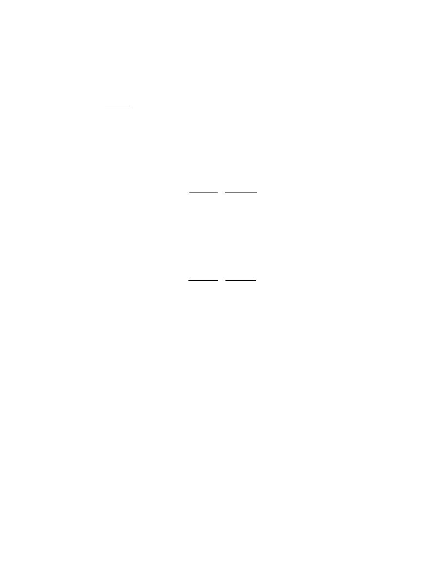
Excerpts from this work may be reproduced by instructors for distribution on a not-for-profit basis for testing or instructional purposes only to
students enrolled in courses for which the textbook has been adopted. Any other reproduction or translation of this work beyond that permitted
by Sections 107 or 108 of the 1976 United States Copyright Act without the permission of the copyright owner is unlawful.
9.21 Is it possible to have a copper-silver alloy of composition 50 wt% Ag-50 wt% Cu, which, at
equilibrium, consists of
α and β phases having mass fractions W
α
= 0.60 and W
β
= 0.40? If so, what will be the
approximate temperature of the alloy? If such an alloy is not possible, explain why.
Solution
It is not possible to have a Cu-Ag alloy of composition 50 wt% Ag-50 wt% Cu which consists of mass
fractions W
α
= 0.60 and W
β
= 0.40. Using the appropriate phase diagram, Figure 9.7, and, using Equations 9.1 and
9.2 let us determine W
α
and W
β
at just below the eutectic temperature and also at room temperature. At just below
the eutectic, C
α
= 8.0 wt% Ag and C
β
= 91.2 wt% Ag; thus,
W
α
=
C
β
−
C0
C
β
−
C
α
=
91.2
− 50
91.2
− 8
= 0.50
W
β
=1.00
− W
α
= 1.00
− 0.50 = 0.50
Furthermore, at room temperature, C
α
= 0 wt% Ag and C
β
= 100 wt% Ag; employment of Equations 9.1 and 9.2
yields
W
α
=
C
β
− C
0
C
β
− C
α
=
100
− 50
100
− 0
= 0.50
And, W
β
= 0.50. Thus, the mass fractions of the
α and β phases, upon cooling through the α + β phase region will
remain approximately constant at about 0.5, and will never have values of W
α
= 0.60 and W
β
= 0.40 as called for in
the problem.

Excerpts from this work may be reproduced by instructors for distribution on a not-for-profit basis for testing or instructional purposes only to
students enrolled in courses for which the textbook has been adopted. Any other reproduction or translation of this work beyond that permitted
by Sections 107 or 108 of the 1976 United States Copyright Act without the permission of the copyright owner is unlawful.
9.22 For 11.20 kg of a magnesium-lead alloy of composition 30 wt% Pb-70 wt% Mg, is it possible, at
equilibrium, to have
α and Mg
2
Pb phases having respective masses of 7.39 kg and 3.81 kg? If so, what will be the
approximate temperature of the alloy? If such an alloy is not possible, explain why.
Solution
Yes, it is possible to have a 30 wt% Pb-70 wt% Mg alloy which has masses of 7.39 kg and 3.81 kg for the
α and Mg
2
Pb phases, respectively. In order to demonstrate this, it is first necessary to determine the mass fraction
of each phase as follows:
W
α
=
m
α
m
α
+ m
Mg
2
Pb
=
7.39 kg
7.39 kg
+ 3.81 kg
= 0.66
W
Mg
2
Pb
= 1.00
− 0.66 = 0.34
Now, if we apply the lever rule expression for W
α
W
α
=
C
Mg
2
Pb
− C
0
C
Mg
2
Pb
− C
α
Since the Mg
2
Pb phase exists only at 81 wt% Pb, and C
0
= 30 wt% Pb
W
α
= 0.66 =
81
− 30
81
− C
α
Solving for C
α
from this expression yields C
α
= 3.7 wt% Pb. The position along the
α−(α + Mg
2
Pb) phase
boundary of Figure 9.20 corresponding to this composition is approximately 190
°C.

Excerpts from this work may be reproduced by instructors for distribution on a not-for-profit basis for testing or instructional purposes only to
students enrolled in courses for which the textbook has been adopted. Any other reproduction or translation of this work beyond that permitted
by Sections 107 or 108 of the 1976 United States Copyright Act without the permission of the copyright owner is unlawful.
9.23 Derive Equations 9.6a and 9.7a, which may be used to convert mass fraction to volume fraction, and
vice versa.
Solution
This portion of the problem asks that we derive Equation 9.6a, which is used to convert from phase weight
fraction to phase volume fraction. Volume fraction of phase
α, V
α
, is defined by Equation 9.5 as
V
α
=
v
α
v
α
+ v
β
(9.S1)
where
vα
and
vβ
are the volumes of the respective phases in the alloy. Furthermore, the density of each phase is
equal to the ratio of its mass and volume, or upon rearrangement
v
α
=
m
α
ρ
α
(9.S2a)
v
β
=
m
β
ρ
β
(9.S2b)
Substitution of these expressions into Equation 9.S1 leads to
V
α
=
m
α
ρ
α
m
α
ρ
α
+
m
β
ρ
β
(9.S3)
in which m's and
ρ's denote masses and densities, respectively. Now, the mass fractions of the α and β phases (i.e.,
W
α
and W
β
) are defined in terms of the phase masses as
W
α
=
m
α
m
α
+ m
β
(9.S4a)
W
β
=
m
β
m
α
+ m
β
(9.S4b)
Which, upon rearrangement yield

Excerpts from this work may be reproduced by instructors for distribution on a not-for-profit basis for testing or instructional purposes only to
students enrolled in courses for which the textbook has been adopted. Any other reproduction or translation of this work beyond that permitted
by Sections 107 or 108 of the 1976 United States Copyright Act without the permission of the copyright owner is unlawful.
m
α
= W
α
(
m
α
+ m
β
)
(9.S5a)
m
β
= W
β
(
m
α
+ m
β
)
(9.S5b)
Incorporation of these relationships into Equation 9.S3 leads to
V
α
=
W
α
(
m
α
+ m
β
)
ρ
α
W
α
(
m
α
+ m
β
)
ρ
α
+
W
β
(
m
α
+ m
β
)
ρ
β
V
α
=
W
α
ρ
α
W
α
ρ
α
+
W
β
ρ
β
(9.S6)
which is the desired equation.
For this portion of the problem we are asked to derive Equation 9.7a, which is used to convert from phase
volume fraction to mass fraction. Mass fraction of the
α phase is defined as
W
α
=
m
α
m
α
+ m
β
(9.S7)
From Equations 9.S2a and 9.S2b
m
α
= v
α
ρ
α
(9.S8a)
m
β
= v
β
ρ
β
(9.S8b)
Substitution of these expressions into Equation 9.S7 yields
W
α
=
v
α
ρ
α
v
α
ρ
α
+ v
β
ρ
β
(9.S9)

Excerpts from this work may be reproduced by instructors for distribution on a not-for-profit basis for testing or instructional purposes only to
students enrolled in courses for which the textbook has been adopted. Any other reproduction or translation of this work beyond that permitted
by Sections 107 or 108 of the 1976 United States Copyright Act without the permission of the copyright owner is unlawful.
From Equation 9.5 and its equivalent for V
β
the following may be written:
v
α
= V
α
(
v
α
+ v
β
)
(9.S10a)
v
β
= V
β
(
v
α
+ v
β
)
(9.S10b)
Substitution of Equations 9.S10a and 9.S10b into Equation 9.S9 yields
W
α
=
V
α
(
v
α
+ v
β
)
ρ
α
V
α
(
v
α
+ v
β
)
ρ
α
+ V
β
(
v
α
+ v
β
)
ρ
β
W
α
=
V
α
ρ
α
V
α
ρ
α
+ V
β
ρ
β
(9.S11)
which is the desired expression.

Excerpts from this work may be reproduced by instructors for distribution on a not-for-profit basis for testing or instructional purposes only to
students enrolled in courses for which the textbook has been adopted. Any other reproduction or translation of this work beyond that permitted
by Sections 107 or 108 of the 1976 United States Copyright Act without the permission of the copyright owner is unlawful.
9.24 Determine the relative amounts (in terms of volume fractions) of the phases for the alloys and
temperatures given in Problem 9.8a, b, and c. Below are given the approximate densities of the various metals at
the alloy temperatures:
Metal
Temperature (°C)
Density (g/cm
3
)
Ag
900
9.97
Cu
400
8.77
Cu
900
8.56
Pb
175
11.20
Sn
175
7.22
Zn
400
6.83
Solution
This problem asks that we determine the phase volume fractions for the alloys and temperatures in
Problems 9.8a, b, and c. This is accomplished by using the technique illustrated in Example Problem 9.3, and also
the results of Problems 9.8 and 9.14.
(a) This is a Cu-Zn alloy at 400
°C, wherein
C
ε
= 87 wt% Zn-13 wt% Cu
C
η
= 97 wt% Zn-3 wt% Cu
W
ε
= 0.70
W
η
= 0.30
ρ
Cu
= 8.77 g/cm
3
ρ
Zn
= 6.83 g/cm
3
Using these data it is first necessary to compute the densities of the
ε and η phases using Equation 4.10a.
Thus
ρε =
100
C
Zn(
ε
)
ρ
Zn
+
C
Cu(
ε
)
ρ
Cu

Excerpts from this work may be reproduced by instructors for distribution on a not-for-profit basis for testing or instructional purposes only to
students enrolled in courses for which the textbook has been adopted. Any other reproduction or translation of this work beyond that permitted
by Sections 107 or 108 of the 1976 United States Copyright Act without the permission of the copyright owner is unlawful.
=
100
87
6.83 g/cm
3
+
13
8.77 g/cm
3
= 7.03 g/cm
3
ρ
η
=
100
C
Zn(
η)
ρ
Zn
+
C
Cu(
η)
ρ
Cu
=
100
97
6.83 g/cm
3
+
3
8.77 g/cm
3
= 6.88 g/cm
3
Now we may determine the V
ε
and V
η
values using Equation 9.6. Thus,
Vε =
Wε
ρε
Wε
ρε
+
W
η
ρ
η
=
0.70
7.03 g/cm
3
0.70
7.03 g/cm
3
+
0.30
6.88 g/cm
3
= 0.70
Vη =
Wη
ρη
Wε
ρε
+
Wη
ρη
=
0.30
6.88 g/cm
3
0.70
7.03 g/cm
3
+
0.30
6.88 g/cm
3
= 0.30
(b) This is a Pb-Sn alloy at 175
°C, wherein
C
α
= 16 wt% Sn-84 wt% Pb
C
β
= 97 wt% Sn-3 wt% Pb

Excerpts from this work may be reproduced by instructors for distribution on a not-for-profit basis for testing or instructional purposes only to
students enrolled in courses for which the textbook has been adopted. Any other reproduction or translation of this work beyond that permitted
by Sections 107 or 108 of the 1976 United States Copyright Act without the permission of the copyright owner is unlawful.
W
α
= 0.27
W
β
= 0.73
ρ
Sn
= 7.22 g/cm
3
ρ
Pb
= 11.20 g/cm
3
Using this data it is first necessary to compute the densities of the
α and β phases. Thus
ρ
α
=
100
C
Sn(
α)
ρ
Sn
+
C
Pb(
α)
ρ
Pb
=
100
16
7.22 g/cm
3
+
84
11.20 g/cm
3
= 10.29 g/cm
3
ρ
β
=
100
C
Sn(
β)
ρ
Sn
+
C
Pb(
β)
ρ
Pb
=
100
97
7.22 g/cm
3
+
3
11.20 g/cm
3
= 7.30 g/cm
3
Now we may determine the V
α
and V
β
values using Equation 9.6. Thus,
V
α
=
W
α
ρ
α
W
α
ρ
α
+
W
β
ρ
β
=
0.27
10.29 g/cm
3
0.27
10.29 g/cm
3
+
0.73
7.30 g/cm
3
= 0.21
V
β
=
W
β
ρ
β
W
α
ρ
α
+
W
β
ρ
β

Excerpts from this work may be reproduced by instructors for distribution on a not-for-profit basis for testing or instructional purposes only to
students enrolled in courses for which the textbook has been adopted. Any other reproduction or translation of this work beyond that permitted
by Sections 107 or 108 of the 1976 United States Copyright Act without the permission of the copyright owner is unlawful.
=
0.73
7.30 g/cm
3
0.27
10.29 g/cm
3
+
0.73
7.30 g/cm
3
= 0.79
(c) This is a Ag-Cu alloy at 900
°C, wherein only the liquid phase is present. Therefore, V
L
= 1.0.

Excerpts from this work may be reproduced by instructors for distribution on a not-for-profit basis for testing or instructional purposes only to
students enrolled in courses for which the textbook has been adopted. Any other reproduction or translation of this work beyond that permitted
by Sections 107 or 108 of the 1976 United States Copyright Act without the permission of the copyright owner is unlawful.
Development of Microstructure in Isomorphous Alloys
9.25 (a) Briefly describe the phenomenon of coring and why it occurs.
(b) Cite one undesirable consequence of coring.
Solution
(a) Coring is the phenomenon whereby concentration gradients exist across grains in polycrystalline
alloys, with higher concentrations of the component having the lower melting temperature at the grain boundaries.
It occurs, during solidification, as a consequence of cooling rates that are too rapid to allow for the maintenance of
the equilibrium composition of the solid phase.
(b) One undesirable consequence of a cored structure is that, upon heating, the grain boundary regions will
melt first and at a temperature below the equilibrium phase boundary from the phase diagram; this melting results
in a loss in mechanical integrity of the alloy.

Excerpts from this work may be reproduced by instructors for distribution on a not-for-profit basis for testing or instructional purposes only to
students enrolled in courses for which the textbook has been adopted. Any other reproduction or translation of this work beyond that permitted
by Sections 107 or 108 of the 1976 United States Copyright Act without the permission of the copyright owner is unlawful.
Mechanical Properties of Isomorphous Alloys
9.26 It is desirable to produce a copper-nickel alloy that has a minimum noncold-worked tensile strength
of 350 MPa (50,750 psi) and a ductility of at least 48%EL. Is such an alloy possible? If so, what must be its
composition? If this is not possible, then explain why.
Solution
From Figure 9.6a, a tensile strength greater than 350 MPa (50,750 psi) is possible for compositions
between about 22.5 and 98 wt% Ni. On the other hand, according to Figure 9.6b, ductilities greater than 48%EL
exist for compositions less than about 8 wt% and greater than about 98 wt% Ni. Therefore, the stipulated criteria are
met only at a composition of 98 wt% Ni.

Excerpts from this work may be reproduced by instructors for distribution on a not-for-profit basis for testing or instructional purposes only to
students enrolled in courses for which the textbook has been adopted. Any other reproduction or translation of this work beyond that permitted
by Sections 107 or 108 of the 1976 United States Copyright Act without the permission of the copyright owner is unlawful.
Binary Eutectic Systems
9.27 A 45 wt% Pb–55 wt% Mg alloy is rapidly quenched to room temperature from an elevated
temperature in such a way that the high-temperature microstructure is preserved. This microstructure is found to
consist of the α phase and Mg
2
Pb, having respective mass fractions of 0.65 and 0.35. Determine the approximate
temperature from which the alloy was quenched.
Solution
We are asked to determine the approximate temperature from which a 45 wt% Pb-55 wt% Mg alloy was
quenched, given the mass fractions of
α and Mg
2
Pb phases. We can write a lever-rule expression for the mass
fraction of the
α phase as
W
α
= 0.65 =
C
Mg
2
Pb
− C
0
C
Mg
2
Pb
− C
α
The value of C
0
is stated as 45 wt% Pb-55 wt% Mg, and C
Mg
2
Pb
is 81 wt% Pb-19 wt% Mg, which is independent
of temperature (Figure 9.20); thus,
0.65 =
81
− 45
81
− C
α
which yields
C
α
= 25.6 wt% Pb
The temperature at which the
α–(α + Mg
2
Pb) phase boundary (Figure 9.20) has a value of 25.6 wt% Pb is about
360
°C (680°F).

Excerpts from this work may be reproduced by instructors for distribution on a not-for-profit basis for testing or instructional purposes only to
students enrolled in courses for which the textbook has been adopted. Any other reproduction or translation of this work beyond that permitted
by Sections 107 or 108 of the 1976 United States Copyright Act without the permission of the copyright owner is unlawful.
Development of Microstructure in Eutectic Alloys
9.28 Briefly explain why, upon solidification, an alloy of eutectic composition forms a microstructure
consisting of alternating layers of the two solid phases.
Solution
Upon solidification, an alloy of eutectic composition forms a microstructure consisting of alternating layers
of the two solid phases because during the solidification atomic diffusion must occur, and with this layered
configuration the diffusion path length for the atoms is a minimum.

Excerpts from this work may be reproduced by instructors for distribution on a not-for-profit basis for testing or instructional purposes only to
students enrolled in courses for which the textbook has been adopted. Any other reproduction or translation of this work beyond that permitted
by Sections 107 or 108 of the 1976 United States Copyright Act without the permission of the copyright owner is unlawful.
9.29 What is the difference between a phase and a microconstituent?
Solution
A “phase” is a homogeneous portion of the system having uniform physical and chemical characteristics,
whereas a “microconstituent” is an identifiable element of the microstructure (that may consist of more than one
phase).

Excerpts from this work may be reproduced by instructors for distribution on a not-for-profit basis for testing or instructional purposes only to
students enrolled in courses for which the textbook has been adopted. Any other reproduction or translation of this work beyond that permitted
by Sections 107 or 108 of the 1976 United States Copyright Act without the permission of the copyright owner is unlawful.
9.30 Is it possible to have a copper-silver alloy in which the mass fractions of primary
β and total β are
0.68 and 0.925, respectively, at 775
°C (1425°F)? Why or why not?
Solution
This problem asks if it is possible to have a Cu-Ag alloy for which the mass fractions of primary
β and
total
β are 0.68 and 0.925, respectively at 775°C. In order to make this determination we need to set up the
appropriate lever rule expression for each of these quantities. From Figure 9.7 and at 775
°C, C
α
= 8.0 wt% Ag, C
β
= 91.2 wt% Ag, and C
eutectic
= 71.9 wt% Ag.
For primary
β
W
β’
=
C
0 −
C
eutectic
C
β Ê−
C
eutectic
=
C
0
−
71.9
91.2
− 71.9
= 0.68
Solving for C
0
gives C
0
= 85 wt% Ag.
Now the analogous expression for total
β
W
β
=
C
0
− C
α
C
β
− C
α
=
C
0
− 8.0
91.2
− 8.0
= 0.925
And this value of C
0
is 85 wt% Ag. Therefore, since these two C
0
values are the same (85 wt% Ag), this alloy is
possible.

Excerpts from this work may be reproduced by instructors for distribution on a not-for-profit basis for testing or instructional purposes only to
students enrolled in courses for which the textbook has been adopted. Any other reproduction or translation of this work beyond that permitted
by Sections 107 or 108 of the 1976 United States Copyright Act without the permission of the copyright owner is unlawful.
9.31 For 6.70 kg of a magnesium-lead alloy, is it possible to have the masses of primary
α and total α of
4.23 kg and 6.00 kg, respectively, at 460
°C (860°F)? Why or why not?
Solution
This problem asks if it is possible to have a Mg-Pb alloy for which the masses of primary
α and total α are
4.23 kg and 6.00 kg, respectively in 6.70 kg total of the alloy at 460
°C. In order to make this determination we first
need to convert these masses to mass fractions. Thus,
W
α'
=
4.23 kg
6.70 kg
= 0.631
W
α
=
6.00 kg
6.70 kg
= 0.896
Next it is necessary to set up the appropriate lever rule expression for each of these quantities. From Figure 9.20
and at 460
°C, C
α
= 41 wt% Pb, C
Mg
2
Pb
= 81 wt% Pb, and C
eutectic
= 66 wt% Pb
For primary
α
W
α'
=
C
eutectic −
C
0
C
eutectic −
C
α
=
66
− C
0
66
− 41
= 0.631
And solving for C
0
gives C
0
= 50.2 wt% Pb.
Now the analogous expression for total
α
W
α
=
C
Mg
2
Pb
− C
0
C
Mg
2
Pb
− C
α
=
81
− C
0
81
− 41
= 0.896
And this value of C
0
is 45.2 wt% Pb. Therefore, since these two C
0
values are different, this alloy is not possible.

Excerpts from this work may be reproduced by instructors for distribution on a not-for-profit basis for testing or instructional purposes only to
students enrolled in courses for which the textbook has been adopted. Any other reproduction or translation of this work beyond that permitted
by Sections 107 or 108 of the 1976 United States Copyright Act without the permission of the copyright owner is unlawful.
9.32 For a copper-silver alloy of composition 25 wt% Ag-75 wt% Cu and at 775
°C (1425°F) do the
following:
(a) Determine the mass fractions of
α and β phases.
(b) Determine the mass fractions of primary
α and eutectic microconstituents.
(c) Determine the mass fraction of eutectic
α.
Solution
(a) This portion of the problem asks that we determine the mass fractions of
α and β phases for an 25 wt%
Ag-75 wt% Cu alloy (at 775
°C). In order to do this it is necessary to employ the lever rule using a tie line that
extends entirely across the
α + β phase field. From Figure 9.7 and at 775°C, C
α
= 8.0 wt% Ag, C
β
= 91.2 wt% Ag,
and C
eutectic
= 71.9 wt% Sn. Therefore, the two lever-rule expressions are as follows:
W
α
=
C
β
− C
0
C
β
− C
α
=
91.2
− 25
91.2
− 8.0
= 0.796
W
β
=
C
0
− C
α
C
β
− C
α
=
25
− 8.0
91.2
− 8.0
= 0.204
(b) Now it is necessary to determine the mass fractions of primary
α and eutectic microconstituents for this
same alloy. This requires us to utilize the lever rule and a tie line that extends from the maximum solubility of Ag
in the
α phase at 775°C (i.e., 8.0 wt% Ag) to the eutectic composition (71.9 wt% Ag). Thus
W
α'
=
C
eutectic Ê
−
C
0
C
eutectic Ê
−
C
α
=
71.9
− 25
71.9
− 8.0
= 0.734
W
e
=
C
0
− C
α
C
eutectic
− C
α
=
25
− 8.0
71.9
− 8.0
= 0.266
(c) And, finally, we are asked to compute the mass fraction of eutectic
α, W
e
α
. This quantity is simply the
difference between the mass fractions of total
α and primary α as
W
e
α
= W
α
– W
α
' = 0.796 – 0.734 = 0.062

Excerpts from this work may be reproduced by instructors for distribution on a not-for-profit basis for testing or instructional purposes only to
students enrolled in courses for which the textbook has been adopted. Any other reproduction or translation of this work beyond that permitted
by Sections 107 or 108 of the 1976 United States Copyright Act without the permission of the copyright owner is unlawful.
9.33 The microstructure of a lead-tin alloy at 180
°C (355°F) consists of primary β and eutectic structures.
If the mass fractions of these two microconstituents are 0.57 and 0.43, respectively, determine the composition of
the alloy.
Solution
Since there is a primary
β microconstituent present, then we know that the alloy composition, C
0
is
between 61.9 and 97.8 wt% Sn (Figure 9.8). Furthermore, this figure also indicates that C
β
= 97.8 wt% Sn and
C
eutectic
= 61.9 wt% Sn. Applying the appropriate lever rule expression for W
β'
W
β'
=
C
0 −
C
eutectic
C
β Ê−
C
eutectic
=
C
0
− 61.9
97.8
− 61.9
= 0.57
and solving for C
0
yields C
0
= 82.4 wt% Sn.

Excerpts from this work may be reproduced by instructors for distribution on a not-for-profit basis for testing or instructional purposes only to
students enrolled in courses for which the textbook has been adopted. Any other reproduction or translation of this work beyond that permitted
by Sections 107 or 108 of the 1976 United States Copyright Act without the permission of the copyright owner is unlawful.
9.34 Consider the hypothetical eutectic phase diagram for metals A and B, which is similar to that for the
lead-tin system, Figure 9.8. Assume that (1)
α and β phases exist at the A and B extremities of the phase diagram,
respectively; (2) the eutectic composition is 47 wt% B-53 wt% A; and (3) the composition of the
β phase at the
eutectic temperature is 92.6 wt% B-7.4 wt% A. Determine the composition of an alloy that will yield primary
α and
total
α mass fractions of 0.356 and 0.693, respectively.
Solution
We are given a hypothetical eutectic phase diagram for which C
eutectic
= 47 wt% B, C
β
= 92.6 wt% B at
the eutectic temperature, and also that W
α'
= 0.356 and W
α
= 0.693; from this we are asked to determine the
composition of the alloy. Let us write lever rule expressions for W
α'
and W
α
W
α
=
C
β Ê
−
C
0
C
β
− C
α
=
92.6
− C
0
92.6
− C
α
= 0.693
W
α'
=
C
eutectic Ê
− C
0
C
eutectic Ê
− C
α
=
47
− C
0
47
− C
α
= 0.356
Thus, we have two simultaneous equations with C
0
and C
α
as unknowns. Solving them for C
0
gives C
0
= 32.6 wt%
B.
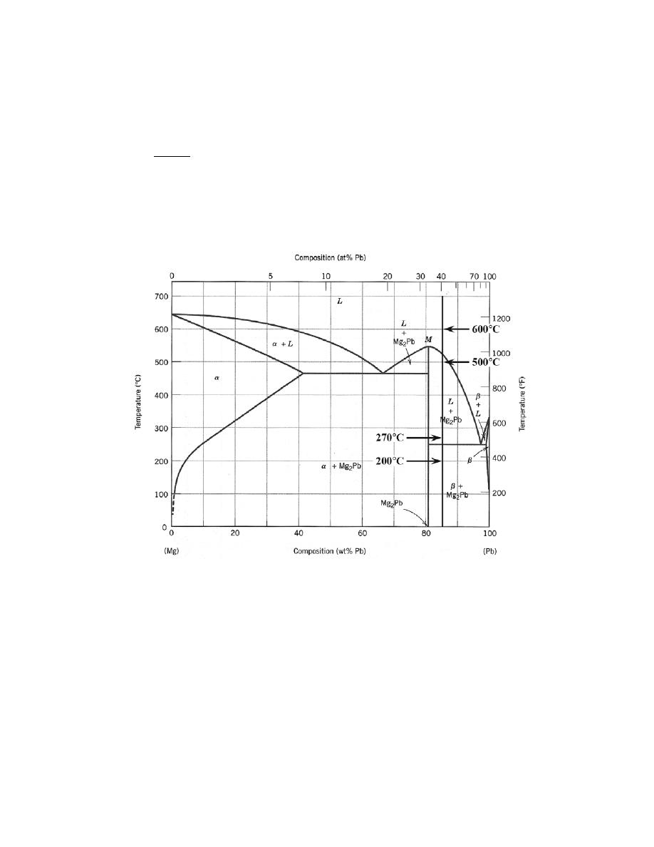
Excerpts from this work may be reproduced by instructors for distribution on a not-for-profit basis for testing or instructional purposes only to
students enrolled in courses for which the textbook has been adopted. Any other reproduction or translation of this work beyond that permitted
by Sections 107 or 108 of the 1976 United States Copyright Act without the permission of the copyright owner is unlawful.
9.35 For an 85 wt% Pb-15 wt% Mg alloy, make schematic sketches of the microstructure that would be
observed for conditions of very slow cooling at the following temperatures: 600
°C (1110°F), 500°C (930°F), 270°C
(520
°F), and 200°C (390°F). Label all phases and indicate their approximate compositions.
Solution
The illustration below is the Mg-Pb phase diagram (Figure 9.20). A vertical line at a composition of 85
wt% Pb-15 wt% Mg has been drawn, and, in addition, horizontal arrows at the four temperatures called for in the
problem statement (i.e., 600
°C, 500°C, 270°C, and 200°C).
On the basis of the locations of the four temperature-composition points, schematic sketches of the four respective
microstructures along with phase compositions are represented as follows:
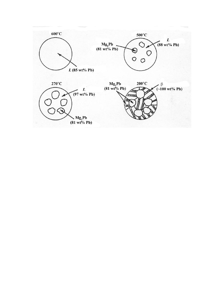
Excerpts from this work may be reproduced by instructors for distribution on a not-for-profit basis for testing or instructional purposes only to
students enrolled in courses for which the textbook has been adopted. Any other reproduction or translation of this work beyond that permitted
by Sections 107 or 108 of the 1976 United States Copyright Act without the permission of the copyright owner is unlawful.
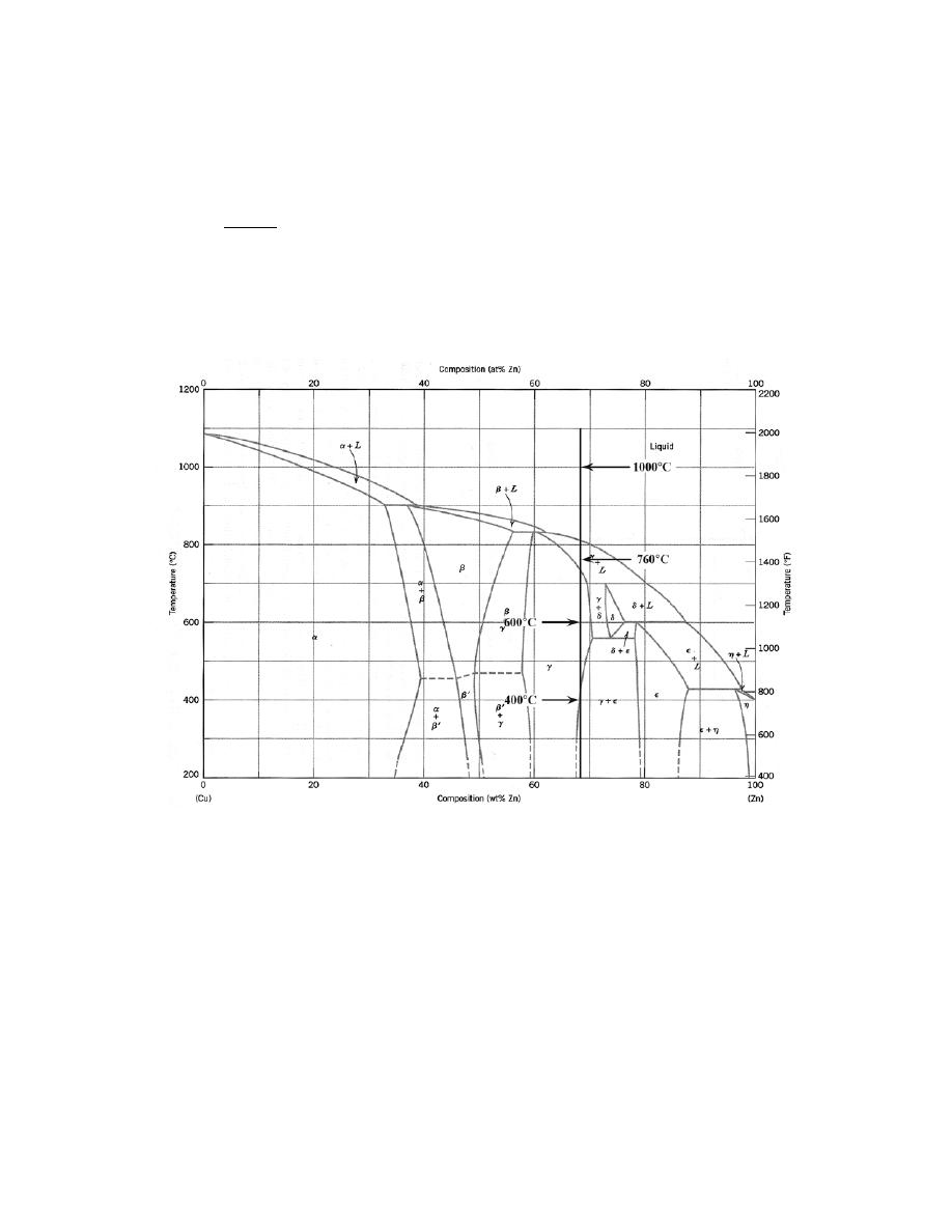
9.36 For a 68 wt% Zn-32 wt% Cu alloy, make schematic sketches of the microstructure that would be
observed for conditions of very slow cooling at the following temperatures: 1000
°C (1830°F), 760°C (1400°F),
600
°C (1110°F), and 400°C (750°F). Label all phases and indicate their approximate compositions.
Solution
The illustration below is the Cu-Zn phase diagram (Figure 9.19). A vertical line at a composition of 68
wt% Zn-32 wt% Cu has been drawn, and, in addition, horizontal arrows at the four temperatures called for in the
problem statement (i.e., 1000
°C, 760°C, 600°C, and 400°C).
On the basis of the locations of the four temperature-composition points, schematic sketches of the four respective
microstructures along with phase compositions are represented as follows:
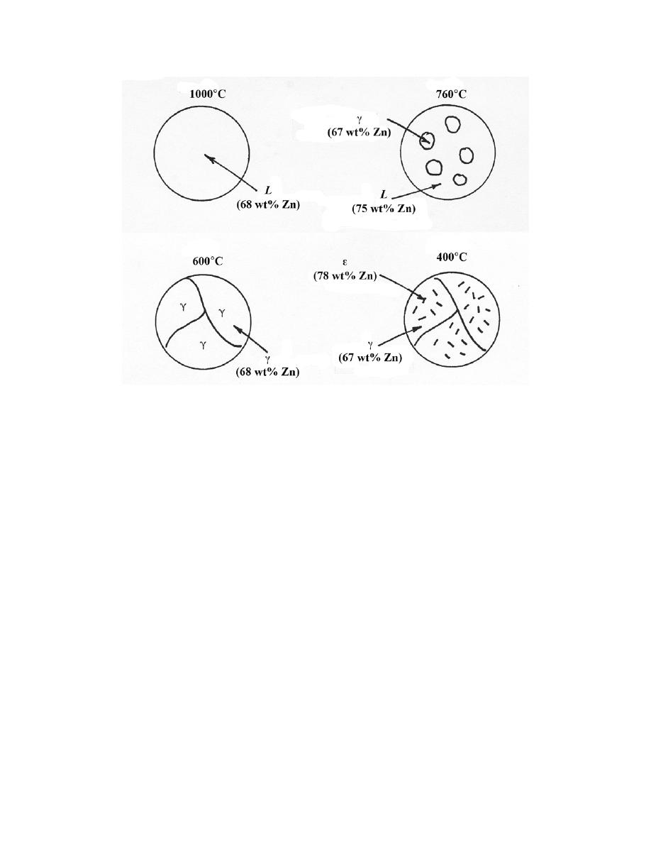
Excerpts from this work may be reproduced by instructors for distribution on a not-for-profit basis for testing or instructional purposes only to
students enrolled in courses for which the textbook has been adopted. Any other reproduction or translation of this work beyond that permitted
by Sections 107 or 108 of the 1976 United States Copyright Act without the permission of the copyright owner is unlawful.
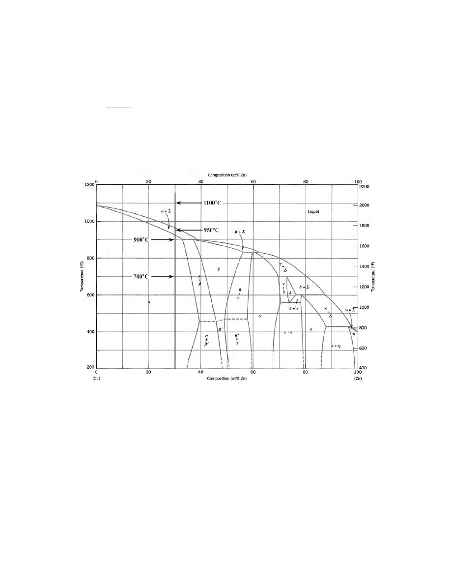
Excerpts from this work may be reproduced by instructors for distribution on a not-for-profit basis for testing or instructional purposes only to
students enrolled in courses for which the textbook has been adopted. Any other reproduction or translation of this work beyond that permitted
by Sections 107 or 108 of the 1976 United States Copyright Act without the permission of the copyright owner is unlawful.
9.37 For a 30 wt% Zn-70 wt% Cu alloy, make schematic sketches of the microstructure that would be
observed for conditions of very slow cooling at the following temperatures: 1100
°C (2010°F), 950°C (1740°F),
900
°C (1650°F), and 700°C (1290°F). Label all phases and indicate their approximate compositions.
Solution
The illustration below is the Cu-Zn phase diagram (Figure 9.19). A vertical line at a composition of 30
wt% Zn-70 wt% Cu has been drawn, and, in addition, horizontal arrows at the four temperatures called for in the
problem statement (i.e., 1100
°C, 950°C, 900°C, and 700°C).
On the basis of the locations of the four temperature-composition points, schematic sketches of the four respective
microstructures along with phase compositions are represented as follows:
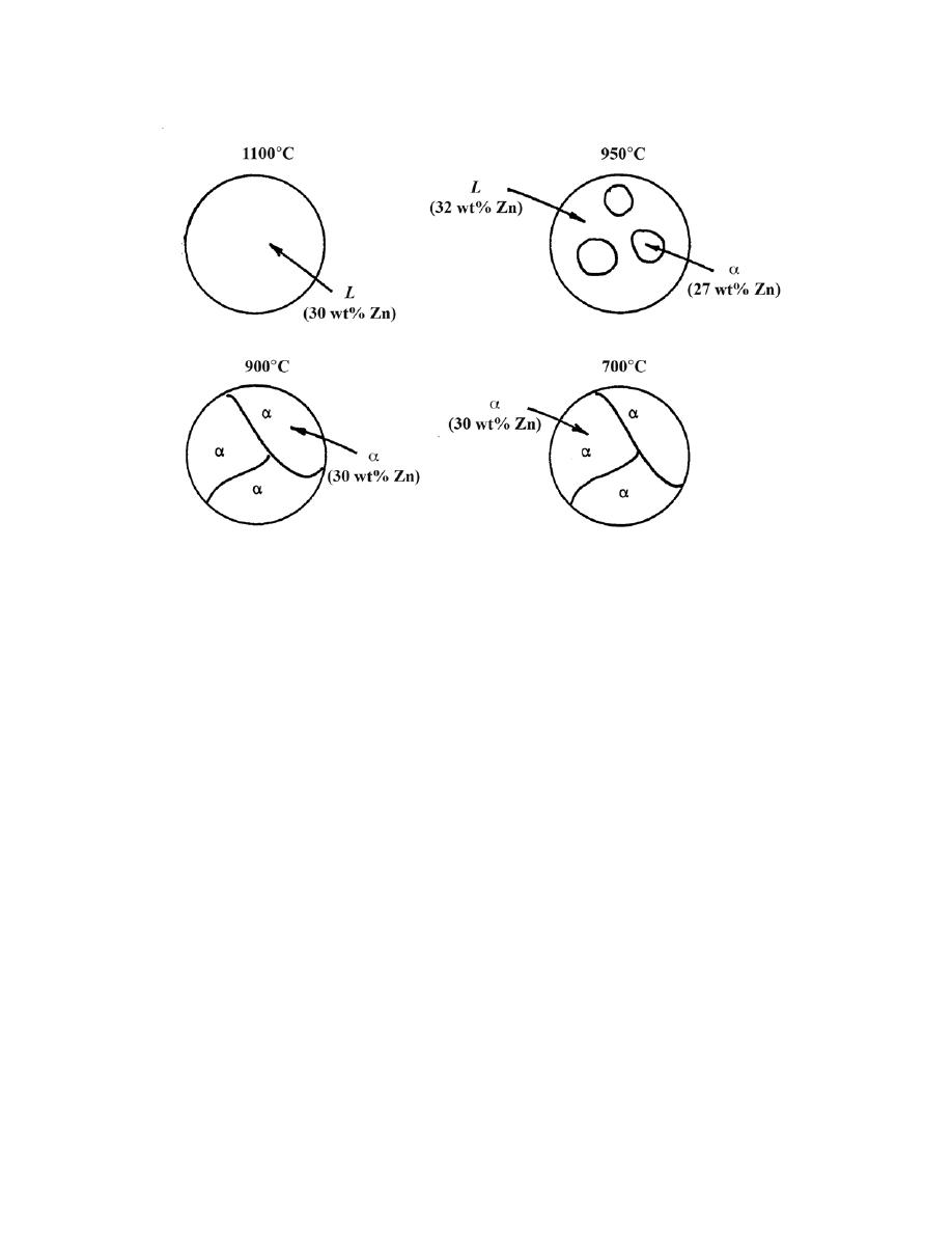
Excerpts from this work may be reproduced by instructors for distribution on a not-for-profit basis for testing or instructional purposes only to
students enrolled in courses for which the textbook has been adopted. Any other reproduction or translation of this work beyond that permitted
by Sections 107 or 108 of the 1976 United States Copyright Act without the permission of the copyright owner is unlawful.
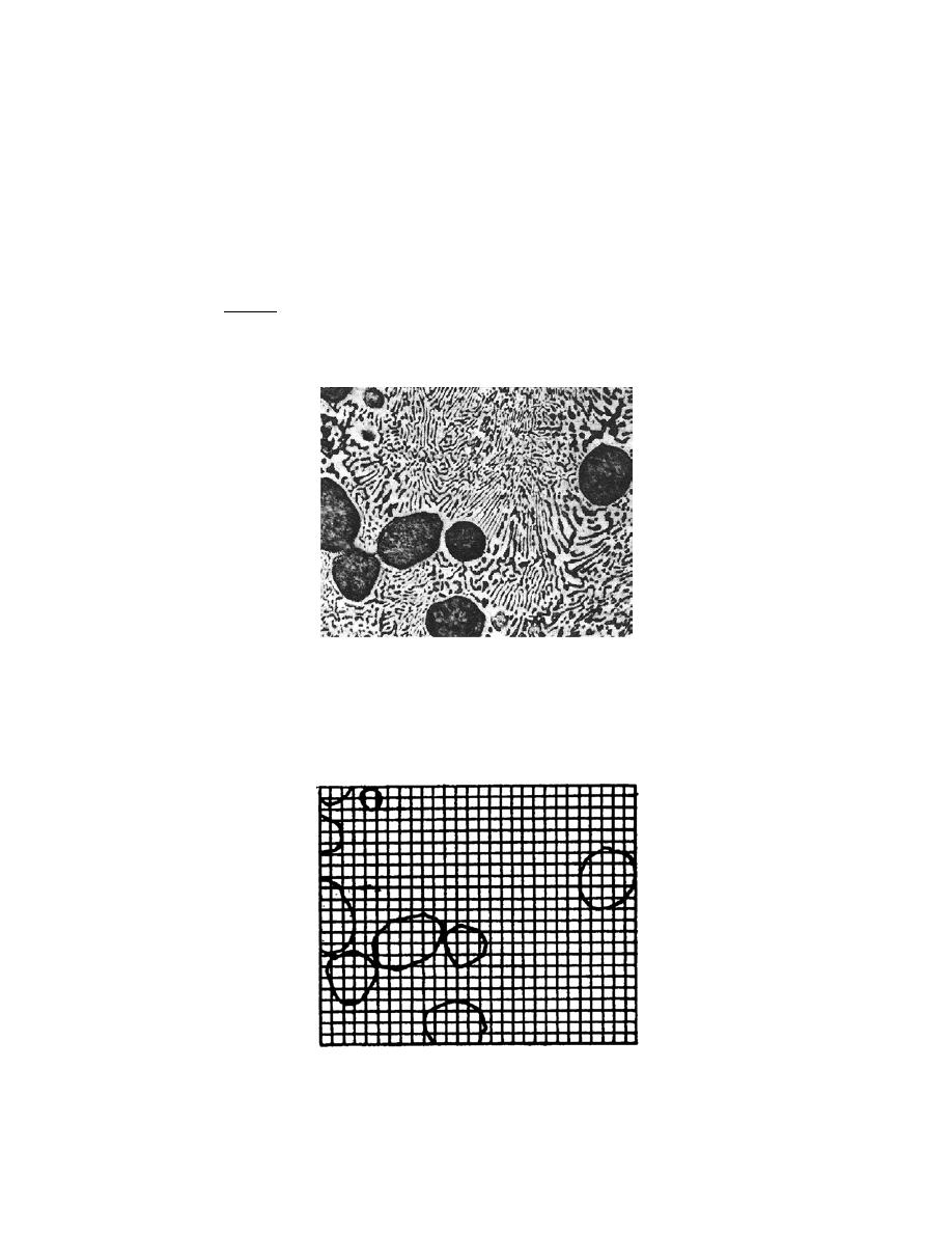
Excerpts from this work may be reproduced by instructors for distribution on a not-for-profit basis for testing or instructional purposes only to
students enrolled in courses for which the textbook has been adopted. Any other reproduction or translation of this work beyond that permitted
by Sections 107 or 108 of the 1976 United States Copyright Act without the permission of the copyright owner is unlawful.
9.38 On the basis of the photomicrograph (i.e., the relative amounts of the microconstituents) for the lead–
tin alloy shown in Figure 9.17 and the Pb–Sn phase diagram (Figure 9.8), estimate the composition of the alloy,
and then compare this estimate with the composition given in the figure legend of Figure 9.17. Make the following
assumptions: (1) the area fraction of each phase and microconstituent in the photomicrograph is equal to its
vol
ume fraction; (2) the densities of the α and β phases as well as the eutectic structure are 11.2, 7.3, and 8.7 g/cm
3
,
respectively; and (3) this photomicrograph represents the equilibrium microstructure at 180°C (355°F).
Solution
Below is shown the micrograph of the Pb-Sn alloy, Figure 9.17:
Primary
α and eutectic microconstituents are present in the photomicrograph, and it is given that their densities are
11.2 and 8.7 g/cm
3
, respectively. Below is shown a square grid network onto which is superimposed outlines of the
primary
α phase areas.

Excerpts from this work may be reproduced by instructors for distribution on a not-for-profit basis for testing or instructional purposes only to
students enrolled in courses for which the textbook has been adopted. Any other reproduction or translation of this work beyond that permitted
by Sections 107 or 108 of the 1976 United States Copyright Act without the permission of the copyright owner is unlawful.
The area fraction of this primary
α phase may be determined by counting squares. There are a total of 644
squares, and of these, approximately 104 lie within the primary
α phase particles. Thus, the area fraction of primary
α is 104/644 = 0.16, which is also assumed to be the volume fraction.
We now want to convert the volume fractions into mass fractions in order to employ the lever rule to the
Pb-Sn phase diagram. To do this, it is necessary to utilize Equations 9.7a and 9.7b as follows:
W
α'
=
V
α'
ρ
α'
V
α'
ρ
α'
+ V
eutectic
ρ
eutectic
=
(0.16)
(
11.2 g /cm
3
)
(0.16)
(
11.2 g /cm
3
)
+ (0.84)
(
8.7 g /cm
3
)
= 0.197
W
eutectic
=
V
eutectic
ρ
eutectic
V
αÕ
ρ
αÕ
+ V
eutectic
ρ
eutectic
=
(0.84)
(
8.7 g /cm
3
)
(0.16)
(
11.2 g /cm
3
)
+ (0.84)
(
8.7 g /cm
3
)
= 0.803
From Figure 9.8, we want to use the lever rule and a tie-line that extends from the eutectic composition (61.9 wt%
Sn) to the
α–(α + β) phase boundary at 180°C (about 18.3 wt% Sn). Accordingly
W
α'
= 0.197 =
61.9
− C
0
61.9
− 18.3
wherein C
0
is the alloy composition (in wt% Sn). Solving for C
0
yields C
0
= 53.3 wt% Sn. This value is in good
agreement with the actual composition—viz. 50 wt% Sn.
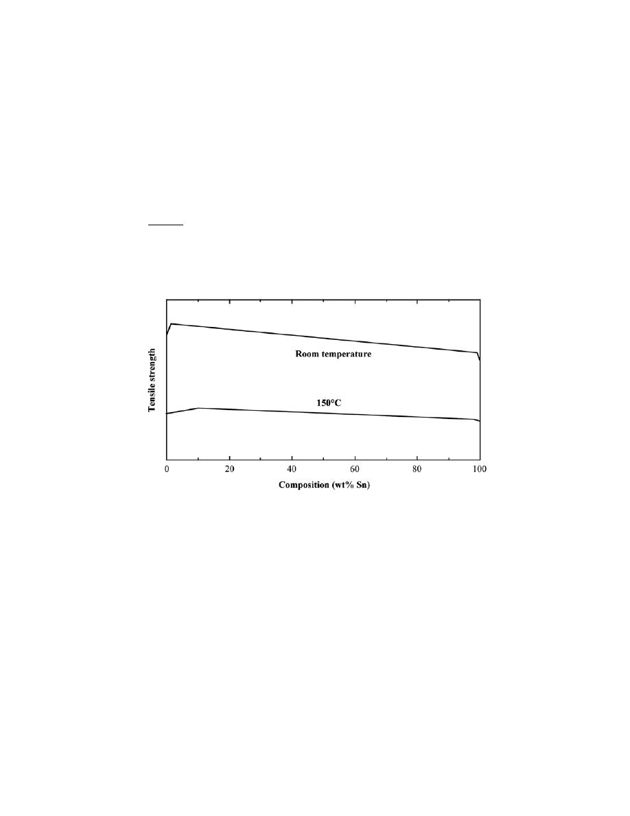
Excerpts from this work may be reproduced by instructors for distribution on a not-for-profit basis for testing or instructional purposes only to
students enrolled in courses for which the textbook has been adopted. Any other reproduction or translation of this work beyond that permitted
by Sections 107 or 108 of the 1976 United States Copyright Act without the permission of the copyright owner is unlawful.
9.39 The room-temperature tensile strengths of pure lead and pure tin are 16.8 MPa and 14.5 MPa,
respectively.
(a) Make a schematic graph of the room-temperature tensile strength versus composition for all
compositions between pure lead and pure tin. (Hint: you may want to consult Sections 9.10 and 9.11, as well as
Equation 9.24 in Problem 9.64.)
(b) On this same graph schematically plot tensile strength versus composition at 150°C.
(c) Explain the shapes of these two curves, as well as any differences between them.
Solution
The (a) and (b) portions of the problem ask that we make schematic plots on the same graph for the tensile
strength versus composition for lead-tin alloys at both room temperature and 150
°C; such a graph is shown below.
(c) Upon consultation of the Pb-Sn phase diagram (Figure 9.8) we note that, at room temperature (20
°C),
about 1.5 wt% of Sn is soluble in Pb (within the
α-phase region at the left extremity of the phase diagram).
Similarly, only about 1 wt% of Pb is soluble in Sn (within the
β-phase region at the left extremity). Thus, there will
a solid-solution strengthening effect on both ends of the phase diagram—strength increases slightly with additions
of Sn to Pb [in the
α phase region (left-hand side)] and with additions of Pb to Sn [in the β phase region (right-hand
side)]; these effects are noted in the above figure. This figure also shows that the tensile strength of pure lead is
greater than pure tin, which is in agreement with tensile strength values provided in the problem statement.
In addition, at room temperature, for compositions between about 1.5 wt% Sn and 99 wt% Sn, both
α and
β phase will coexist, (Figure 9.8), Furthermore, for compositions within this range, tensile strength will depend
(approximately) on the tensile strengths of each of the
α and β phases as well as their phase fractions in a manner
described by Equation 9.24 for the elastic modulus (Problem 9.64). That is, for this problem

Excerpts from this work may be reproduced by instructors for distribution on a not-for-profit basis for testing or instructional purposes only to
students enrolled in courses for which the textbook has been adopted. Any other reproduction or translation of this work beyond that permitted
by Sections 107 or 108 of the 1976 United States Copyright Act without the permission of the copyright owner is unlawful.
(TS)
alloy
≅ (TS)
α
V
α
+ (TS)
β
V
β
in which TS and V denote tensile strength and volume fraction, respectively, and the subscripts represent the
alloy/phases. Also, mass fractions of the
α and β phases change linearly with changing composition (according to
the lever rule). Furthermore, although there is some disparity between the densities of Pb and Sn (11.35 versus 7.27
g/cm
3
), weight and volume fractions of the
α and β phases will also be similar (see Equation 9.6).
At 150
°C, the curve will be shifted to significantly lower tensile strengths inasmuch as tensile strength
diminishes with increasing temperature (Section 6.6, Figure 6.14). In addition, according to Figure 9.8, solubility
limits for both
α and β phases increase—for the α phase from 1.5 to 10 wt% Sn, and for the β phase from 1 to about
2 wt% Pb. Thus, the compositional ranges over which solid-solution strengthening occurs increase somewhat from
the room-temperature ranges; these effects are also noted on the 150
°C curve above. Furthermore, at 150°C, it
would be expected that the tensile strength of lead will be greater than that of tin; and for compositions over which
both
α and β phases coexist, strength will decrease approximately linearly with increasing Sn content.

Excerpts from this work may be reproduced by instructors for distribution on a not-for-profit basis for testing or instructional purposes only to
students enrolled in courses for which the textbook has been adopted. Any other reproduction or translation of this work beyond that permitted
by Sections 107 or 108 of the 1976 United States Copyright Act without the permission of the copyright owner is unlawful.
Equilibrium Diagrams Having Intermediate Phases or Compounds
9.40 Two intermetallic compounds, AB and AB
2
, exist for elements A and B. If the compositions for AB
and AB
2
are 34.3 wt% A–65.7 wt% B and 20.7 wt% A–79.3 wt% B, respectively, and element A is potassium,
identify element B.
Solution
This problem gives us the compositions in weight percent for the two intermetallic compounds AB and
AB
2
, and then asks us to identify element B if element A is potassium. Probably the easiest way to solve this
problem is to first compute the ratio of the atomic weights of these two elements using Equation 4.6a; then, since
we know the atomic weight of potassium (39.10 g/mol, per inside the front cover), it is possible to determine the
atomic weight of element B, from which an identification may be made.
First of all, consider the AB intermetallic compound; inasmuch as it contains the same numbers of A and
B atoms, its composition in atomic percent is 50 at% A-50 at% B. Equation 4.6a may be written in the form:
C
B
'
=
C
B
A
A
C
A
A
B
+ C
B
A
A
× 100
where A
A
and A
B
are the atomic weights for elements A and B, and C
A
and C
B
are their compositions in weight
percent. For this AB compound, and making the appropriate substitutions in the above equation leads to
50 at% B =
(65.7 wt% B)( A
A
)
(34.3 wt% A)( A
B
)
+ (65.7 wt% B)(A
A
)
× 100
Now, solving this expression yields,
A
B
= 1.916 A
A
Since potassium is element A and it has an atomic weight of 39.10 g/mol, the atomic weight of element B is just
A
B
= (1.916)(39.10 g/mol) = 74.92 g/mol
Upon consultation of the period table of the elements (Figure 2.6) we note the element that has an atomic weight
closest to this value is arsenic (74.92 g/mol). Therefore, element B is arsenic, and the two intermetallic compounds
are KAs and KAs
2
.

Excerpts from this work may be reproduced by instructors for distribution on a not-for-profit basis for testing or instructional purposes only to
students enrolled in courses for which the textbook has been adopted. Any other reproduction or translation of this work beyond that permitted
by Sections 107 or 108 of the 1976 United States Copyright Act without the permission of the copyright owner is unlawful.
Congruent Phase Transformations
Eutectoid and Peritectic Reactions
9.41 What is the principal difference between congruent and incongruent phase transformations?
Solution
The principal difference between congruent and incongruent phase transformations is that for congruent no
compositional changes occur with any of the phases that are involved in the transformation. For incongruent there
will be compositional alterations of the phases.
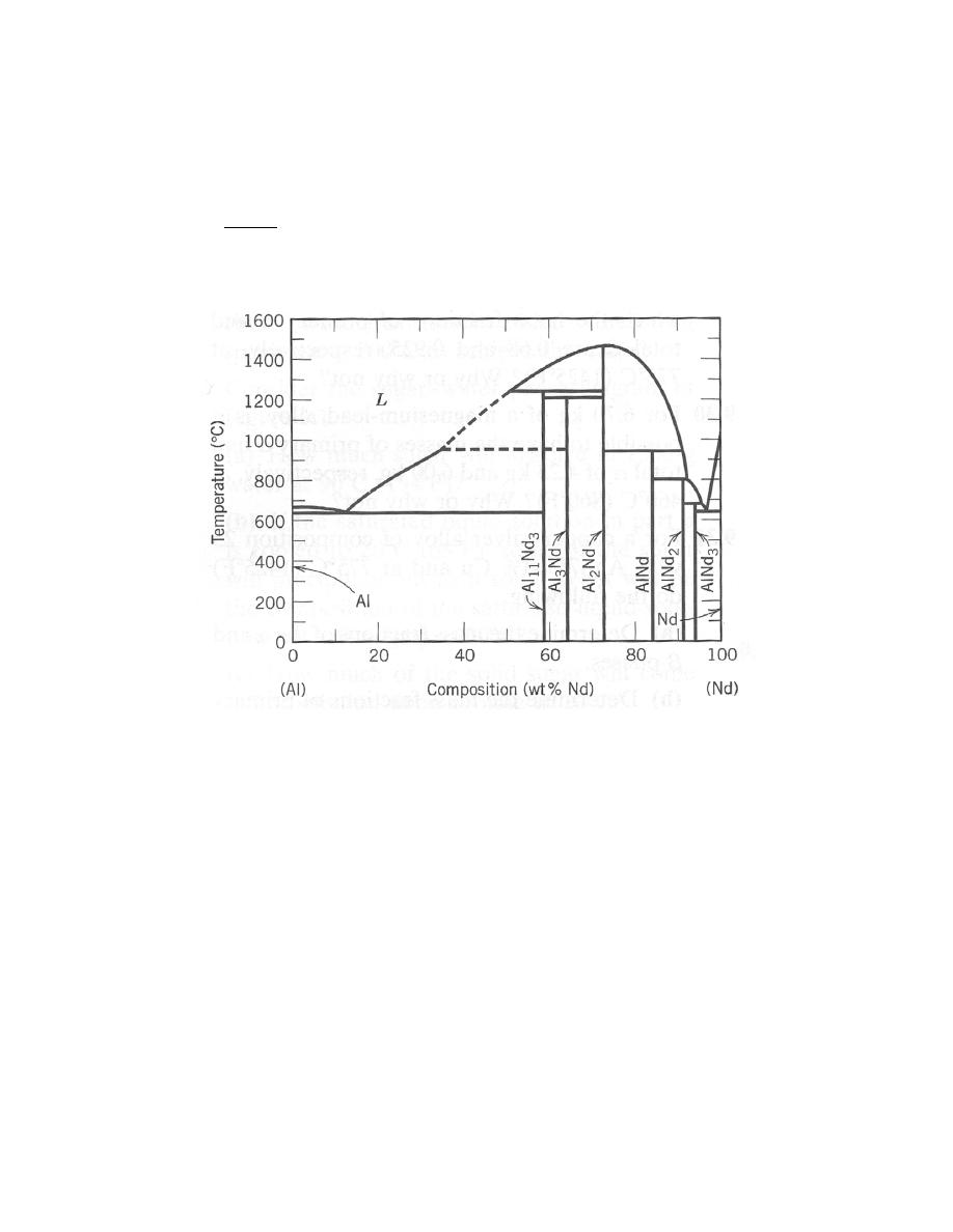
Excerpts from this work may be reproduced by instructors for distribution on a not-for-profit basis for testing or instructional purposes only to
students enrolled in courses for which the textbook has been adopted. Any other reproduction or translation of this work beyond that permitted
by Sections 107 or 108 of the 1976 United States Copyright Act without the permission of the copyright owner is unlawful.
9.42 Figure 9.36 is the aluminum-neodymium phase diagram, for which only single-phase regions are
labeled. Specify temperature-composition points at which all eutectics, eutectoids, peritectics, and congruent phase
transformations occur. Also, for each, write the reaction upon cooling.
Solution
Below is shown the aluminum-neodymium phase diagram (Figure 9.36).
There are two eutectics on this phase diagram. One exists at 12 wt% Nd-88 wt% Al and 632
°C. The
reaction upon cooling is
L
→ Al + Al
11
Nd
3
The other eutectic exists at about 97 wt% Nd-3 wt% Al and 635
°C. This reaction upon cooling is
L
→ AlNd
3
+ Nd
There are four peritectics. One exists at 59 wt% Nd-41 wt% Al and 1235
°C. Its reaction upon cooling is
as follows:

Excerpts from this work may be reproduced by instructors for distribution on a not-for-profit basis for testing or instructional purposes only to
students enrolled in courses for which the textbook has been adopted. Any other reproduction or translation of this work beyond that permitted
by Sections 107 or 108 of the 1976 United States Copyright Act without the permission of the copyright owner is unlawful.
L + Al
2
Nd
→ Al
11
Nd
3
The second peritectic exists at 84 wt% Nd-16 wt% Al and 940
°C. This reaction upon cooling is
L + Al
2
Nd
→ AlNd
The third peritectic exists at 91 wt% Nd-9 wt% Al and 795
°C. This reaction upon cooling is
L + AlNd
→ AlNd
2
The fourth peritectic exists at 94 wt% Nd-6 wt% Al and 675
°C. This reaction upon cooling is
L + AlNd
2
→ AlNd
3
There is one congruent melting point at about 73 wt% Nd-27 wt% Al and 1460
°C. Its reaction upon
cooling is
L
→ Al
2
Nd
No eutectoids are present.
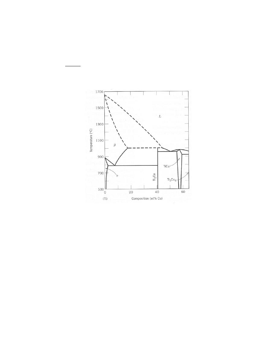
Excerpts from this work may be reproduced by instructors for distribution on a not-for-profit basis for testing or instructional purposes only to
students enrolled in courses for which the textbook has been adopted. Any other reproduction or translation of this work beyond that permitted
by Sections 107 or 108 of the 1976 United States Copyright Act without the permission of the copyright owner is unlawful.
9.43 Figure 9.37 is a portion of the titanium-copper phase diagram for which only single-phase regions
are labeled. Specify all temperature-composition points at which eutectics, eutectoids, peritectics, and congruent
phase transformations occur. Also, for each, write the reaction upon cooling.
Solution
Below is shown the titanium-copper phase diagram (Figure 9.37).
There is one eutectic on this phase diagram, which exists at about 51 wt% Cu-49 wt% Ti and 960
°C. Its
reaction upon cooling is
L
→ Ti
2
Cu + TiCu
There is one eutectoid for this system. It exists at about 7.5 wt% Cu-92.5 wt% Ti and 790
°C. This
reaction upon cooling is
β → α + Ti
2
Cu
There is one peritectic on this phase diagram. It exists at about 40 wt% Cu-60 wt% Ti and 1005
°C. The
reaction upon cooling is

Excerpts from this work may be reproduced by instructors for distribution on a not-for-profit basis for testing or instructional purposes only to
students enrolled in courses for which the textbook has been adopted. Any other reproduction or translation of this work beyond that permitted
by Sections 107 or 108 of the 1976 United States Copyright Act without the permission of the copyright owner is unlawful.
β + L → Ti
2
Cu
There is a single congruent melting point that exists at about 57.5 wt% Cu-42.5 wt% Ti and 982
°C. The
reaction upon cooling is
L
→ TiCu
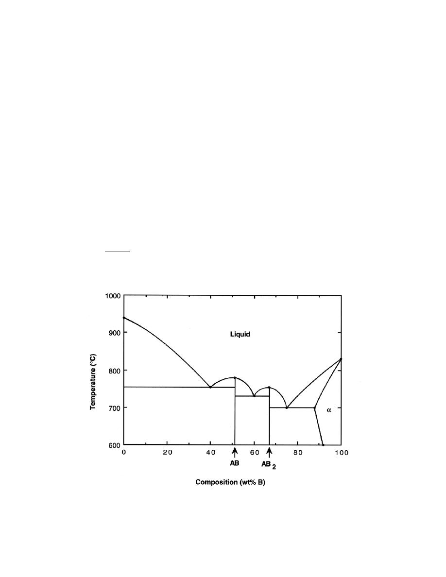
Excerpts from this work may be reproduced by instructors for distribution on a not-for-profit basis for testing or instructional purposes only to
students enrolled in courses for which the textbook has been adopted. Any other reproduction or translation of this work beyond that permitted
by Sections 107 or 108 of the 1976 United States Copyright Act without the permission of the copyright owner is unlawful.
9.44 Construct the hypothetical phase diagram for metals A and B between temperatures of 600
°C and
1000
°C given the following information:
●
The melting temperature of metal A is 940
°C.
●
The solubility of B in A is negligible at all temperatures.
●
The melting temperature of metal B is 830
°C.
●
The maximum solubility of A in B is 12 wt% A, which occurs at 700
°C.
●
At 600
°C, the solubility of A in B is 8 wt% A.
●
One eutectic occurs at 700
°C and 75 wt% B–25 wt% A.
●
A second eutectic occurs at 730
°C and 60 wt% B–40 wt% A.
●
A third eutectic occurs at 755
°C and 40 wt% B–60 wt% A.
●
One congruent melting point occurs at 780
°C and 51 wt% B–49 wt% A.
●
A second congruent melting point occurs at 755
°C and 67 wt% B–33 wt% A.
●
The intermetallic compound AB exists at 51 wt% B–49 wt% A.
●
The intermetallic compound AB
2
exists at 67 wt% B–33 wt% A.
Solution
Below is shown the phase diagram for these two A and B metals.
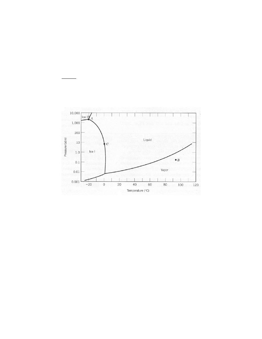
Excerpts from this work may be reproduced by instructors for distribution on a not-for-profit basis for testing or instructional purposes only to
students enrolled in courses for which the textbook has been adopted. Any other reproduction or translation of this work beyond that permitted
by Sections 107 or 108 of the 1976 United States Copyright Act without the permission of the copyright owner is unlawful.
The Gibbs Phase Rule
9.45 In Figure 9.38 is shown the pressure–temperature phase diagram for H
2
O. Apply the Gibbs phase
rule at points A, B, and C; that is, specify the number of degrees of freedom at each of the points—that is, the
number of externally controllable variables that need be specified to completely define the system.
Solution
We are asked to specify the value of F for Gibbs phase rule at points A, B, and C on the pressure-
temperature diagram for H
2
O, Figure 9.38, which is shown below.
Gibbs phase rule in general form is
P + F = C + N
For this system, the number of components, C, is 1, whereas N, the number of noncompositional variables, is 2--viz.
temperature and pressure. Thus, the phase rule now becomes
P + F = 1 + 2 = 3
Or
F = 3 – P
where P is the number of phases present at equilibrium.

Excerpts from this work may be reproduced by instructors for distribution on a not-for-profit basis for testing or instructional purposes only to
students enrolled in courses for which the textbook has been adopted. Any other reproduction or translation of this work beyond that permitted
by Sections 107 or 108 of the 1976 United States Copyright Act without the permission of the copyright owner is unlawful.
At point A, three phases are present (viz. ice I, ice III, and liquid) and P = 3; thus, the number of degrees
of freedom is zero since
F = 3 – P = 3 – 3 = 0
Thus, point A is an invariant point (in this case a triple point), and we have no choice in the selection of externally
controllable variables in order to define the system.
At point B on the figure, only a single (vapor) phase is present (i.e., P = 1), or
F = 3 – P = 3 – 1 = 2
which means that specification of both temperature and pressure are necessary to define the system.
And, finally, at point C which is on the phase boundary between liquid and ice I phases, two phases are in
equilibrium (P = 2); hence
F = 3 – P = 3 – 2 = 1
Or that we need to specify the value of either temperature or pressure, which determines the value of the other
parameter (pressure or temperature).

Excerpts from this work may be reproduced by instructors for distribution on a not-for-profit basis for testing or instructional purposes only to
students enrolled in courses for which the textbook has been adopted. Any other reproduction or translation of this work beyond that permitted
by Sections 107 or 108 of the 1976 United States Copyright Act without the permission of the copyright owner is unlawful.
The Iron-Iron Carbide (Fe-Fe3C) Phase Diagram
Development of Microstructure in Iron-Carbon Alloys
9.46
Compute the mass fractions of α ferrite and cementite in pearlite.
Solution
This problem asks that we compute the mass fractions of
α ferrite and cementite in pearlite. The lever-rule
expression for ferrite is
W
α
=
C
Fe
3
C
− C
0
C
Fe
3
C
− C
α
and, since C
Fe
3
C
= 6.70 wt% C, C
0
= 0.76 wt% C, and C
α
= 0.022 wt% C
W
α
=
6.70
− 0.76
6.70
− 0.022
= 0.89
Similarly, for cementite
W
Fe
3
C
=
C
0
− C
α
C
Fe
3
C
− C
α
=
0.76
− 0.022
6.70
− 0.022
= 0.11

Excerpts from this work may be reproduced by instructors for distribution on a not-for-profit basis for testing or instructional purposes only to
students enrolled in courses for which the textbook has been adopted. Any other reproduction or translation of this work beyond that permitted
by Sections 107 or 108 of the 1976 United States Copyright Act without the permission of the copyright owner is unlawful.
9.47 (a) What is the distinction between hypoeutectoid and hypereutectoid steels?
(b) In a hypoeutectoid steel, both eutectoid and proeutectoid ferrite exist. Explain the difference between
them. What will be the carbon concentration in each?
Solution
(a) A “hypoeutectoid” steel has a carbon concentration less than the eutectoid; on the other hand, a
“hypereutectoid” steel has a carbon content greater than the eutectoid.
(b) For a hypoeutectoid steel, the proeutectoid ferrite is a microconstituent that formed above the eutectoid
temperature. The eutectoid ferrite is one of the constituents of pearlite that formed at a temperature below the
eutectoid. The carbon concentration for both ferrites is 0.022 wt% C.

Excerpts from this work may be reproduced by instructors for distribution on a not-for-profit basis for testing or instructional purposes only to
students enrolled in courses for which the textbook has been adopted. Any other reproduction or translation of this work beyond that permitted
by Sections 107 or 108 of the 1976 United States Copyright Act without the permission of the copyright owner is unlawful.
9.48 What is the carbon concentration of an iron–carbon alloy for which the fraction of total ferrite is
0.94?
Solution
This problem asks that we compute the carbon concentration of an iron-carbon alloy for which the fraction
of total ferrite is 0.94. Application of the lever rule (of the form of Equation 9.12) yields
W
α
= 0.94 =
C
Fe
3
C
− C
0
'
C
Fe
3
C
− C
α
=
6.70
− C
0
'
6.70
− 0.022
and solving for
C
0
'
C
0
'
= 0.42 wt% C

Excerpts from this work may be reproduced by instructors for distribution on a not-for-profit basis for testing or instructional purposes only to
students enrolled in courses for which the textbook has been adopted. Any other reproduction or translation of this work beyond that permitted
by Sections 107 or 108 of the 1976 United States Copyright Act without the permission of the copyright owner is unlawful.
9.49 What is the proeutectoid phase for an iron–carbon alloy in which the mass fractions of total ferrite
and total cementite are 0.92 and 0.08, respectively? Why?
Solution
In this problem we are given values of W
α
and W
Fe
3
C
(0.92 and 0.08, respectively) for an iron-carbon
alloy and then are asked to specify the proeutectoid phase. Employment of the lever rule for total
α leads to
W
α
= 0.92 =
C
Fe
3
C
− C
0
C
Fe
3
C
− C
α
=
6.70
− C
0
6.70
− 0.022
Now, solving for C
0
, the alloy composition, leads to C
0
= 0.56 wt% C. Therefore, the proeutectoid phase is
α-
ferrite since C
0
is less than 0.76 wt% C.

Excerpts from this work may be reproduced by instructors for distribution on a not-for-profit basis for testing or instructional purposes only to
students enrolled in courses for which the textbook has been adopted. Any other reproduction or translation of this work beyond that permitted
by Sections 107 or 108 of the 1976 United States Copyright Act without the permission of the copyright owner is unlawful.
9.50 Consider 1.0 kg of austenite containing 1.15 wt% C, cooled to below 727
°C (1341°F).
(a) What is the proeutectoid phase?
(b) How many kilograms each of total ferrite and cementite form?
(c) How many kilograms each of pearlite and the proeutectoid phase form?
(d) Schematically sketch and label the resulting microstructure.
Solution
(a) The proeutectoid phase will be Fe
3
C since 1.15 wt% C is greater than the eutectoid composition (0.76
wt% C).
(b) For this portion of the problem, we are asked to determine how much total ferrite and cementite form.
Application of the appropriate lever rule expression yields
W
α
=
C
Fe
3
C
− C
0
C
Fe
3
C
− C
α
=
6.70
− 1.15
6.70
− 0.022
= 0.83
which, when multiplied by the total mass of the alloy (1.0 kg), gives 0.83 kg of total ferrite.
Similarly, for total cementite,
W
Fe
3
C
=
C
0
− C
α
C
Fe
3
C
− C
α
=
1.15
− 0.022
6.70
− 0.022
= 0.17
And the mass of total cementite that forms is (0.17)(1.0 kg) = 0.17 kg.
(c) Now we are asked to calculate how much pearlite and the proeutectoid phase (cementite) form.
Applying Equation 9.22, in which
C
1
'
= 1.15 wt% C
W
p
=
6.70
− C
1
'
6.70
− 0.76
=
6.70
− 1.15
6.70
− 0.76
= 0.93
which corresponds to a mass of 0.93 kg. Likewise, from Equation 9.23
W
Fe
3
C'
=
C
1
'
− 0.76
5.94
=
1.15
− 0.76
5.94
= 0.07
which is equivalent to 0.07 kg of the total 1.0 kg mass.
(d) Schematically, the microstructure would appear as:
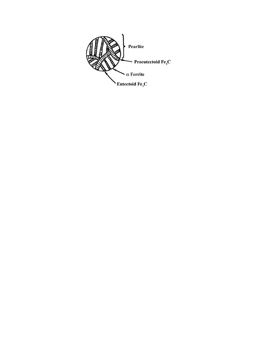
Excerpts from this work may be reproduced by instructors for distribution on a not-for-profit basis for testing or instructional purposes only to
students enrolled in courses for which the textbook has been adopted. Any other reproduction or translation of this work beyond that permitted
by Sections 107 or 108 of the 1976 United States Copyright Act without the permission of the copyright owner is unlawful.
9.51 Consider 2.5 kg of austenite containing 0.65 wt% C, cooled to below 727
°C (1341°F).
(a) What is the proeutectoid phase?
(b) How many kilograms each of total ferrite and cementite form?
(c) How many kilograms each of pearlite and the proeutectoid phase form?
(d) Schematically sketch and label the resulting microstructure.
Solution
(a) Ferrite is the proeutectoid phase since 0.65 wt% C is less than 0.76 wt% C.
(b) For this portion of the problem, we are asked to determine how much total ferrite and cementite form.
For ferrite, application of the appropriate lever rule expression yields
W
α
=
C
Fe
3
C
− C
0
C
Fe
3
C
− C
α
=
6.70
− 0.65
6.70
− 0.022
= 0.91
which corresponds to (0.91)(2.5 kg) = 2.27 kg of total ferrite.
Similarly, for total cementite,
W
Fe
3
C
=
C
0
− C
α
C
Fe
3
C
− C
α
=
0.65
− 0.022
6.70
− 0.022
= 0.09
Or (0.09)(2.5 kg) = 0.23 kg of total cementite form.
(c) Now consider the amounts of pearlite and proeutectoid ferrite. Using Equation 9.20
W
p
=
C
0
'
− 0.022
0.74
=
0.65
− 0.022
0.74
= 0.85
This corresponds to (0.85)(2.5 kg) = 2.12 kg of pearlite.
Also, from Equation 9.21,
W
α'
=
0.76
− 0.65
0.74
= 0.15
Or, there are (0.15)(2.5 kg) = 0.38 kg of proeutectoid ferrite.
(d) Schematically, the microstructure would appear as:
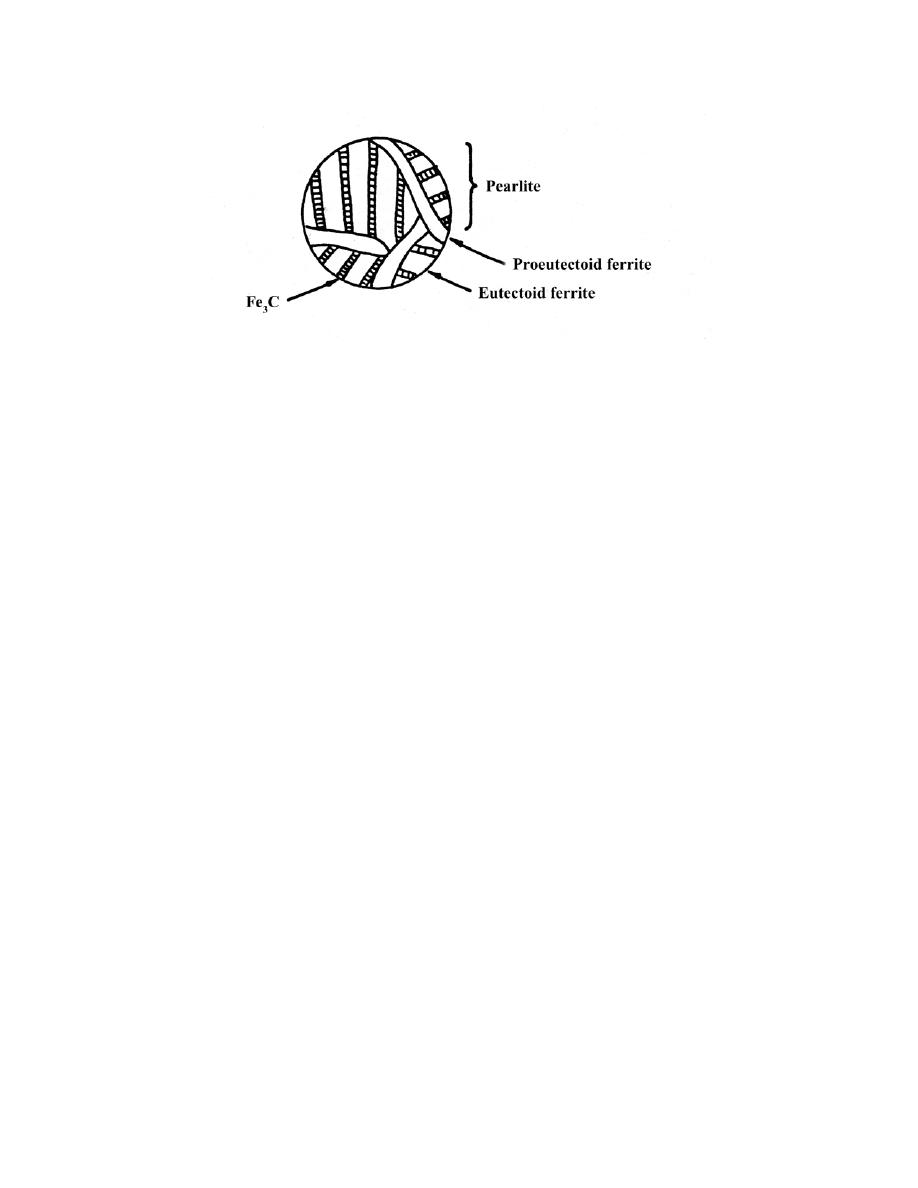
Excerpts from this work may be reproduced by instructors for distribution on a not-for-profit basis for testing or instructional purposes only to
students enrolled in courses for which the textbook has been adopted. Any other reproduction or translation of this work beyond that permitted
by Sections 107 or 108 of the 1976 United States Copyright Act without the permission of the copyright owner is unlawful.

Excerpts from this work may be reproduced by instructors for distribution on a not-for-profit basis for testing or instructional purposes only to
students enrolled in courses for which the textbook has been adopted. Any other reproduction or translation of this work beyond that permitted
by Sections 107 or 108 of the 1976 United States Copyright Act without the permission of the copyright owner is unlawful.
9.52 Compute the mass fractions of proeutectoid ferrite and pearlite that form in an iron–carbon alloy
containing 0.25 wt% C.
Solution
The mass fractions of proeutectoid ferrite and pearlite that form in a 0.25 wt% C iron-carbon alloy are
considered in this problem. From Equation 9.20
W
p
=
C
0
'
− 0.022
0.74
=
0.25
− 0.022
0.74
= 0.31
And, from Equation 9.21 (for proeutectoid ferrite)
W
α'
=
0.76
− C
0
'
0.74
=
0.76
− 0.25
0.74
= 0.69

Excerpts from this work may be reproduced by instructors for distribution on a not-for-profit basis for testing or instructional purposes only to
students enrolled in courses for which the textbook has been adopted. Any other reproduction or translation of this work beyond that permitted
by Sections 107 or 108 of the 1976 United States Copyright Act without the permission of the copyright owner is unlawful.
9.53 The microstructure of an iron–carbon alloy consists of proeutectoid ferrite and pearlite; the mass
fractions of these two microconstituents are 0.286 and 0.714, respectively. Determine the concentration of carbon
in this alloy.
Solution
This problem asks that we determine the carbon concentration in an iron-carbon alloy, given the mass
fractions of proeutectoid ferrite and pearlite. From Equation 9.20
W
p
= 0.714 =
C
0
'
− 0.022
0.74
which yields
C
0
'
= 0.55 wt% C.

Excerpts from this work may be reproduced by instructors for distribution on a not-for-profit basis for testing or instructional purposes only to
students enrolled in courses for which the textbook has been adopted. Any other reproduction or translation of this work beyond that permitted
by Sections 107 or 108 of the 1976 United States Copyright Act without the permission of the copyright owner is unlawful.
9.54 The mass fractions of total ferrite and total cementite in an iron-carbon alloy are 0.88 and 0.12,
respectively. Is this a hypoeutectoid or hypereutectoid alloy? Why?
Solution
In this problem we are given values of W
α
and W
Fe
3
C
for an iron-carbon alloy (0.88 and 0.12,
respectively), and then are asked to specify whether the alloy is hypoeutectoid or hypereutectoid. Employment of
the lever rule for total
α leads to
W
α
= 0.88 =
C
Fe
3
C
− C
0
C
Fe
3
C
− C
α
=
6.70
− C
0
6.70
− 0.022
Now, solving for C
0
, the alloy composition, leads to C
0
= 0.82 wt% C. Therefore, the alloy is hypereutectoid since
C
0
is greater than 0.76 wt% C.

Excerpts from this work may be reproduced by instructors for distribution on a not-for-profit basis for testing or instructional purposes only to
students enrolled in courses for which the textbook has been adopted. Any other reproduction or translation of this work beyond that permitted
by Sections 107 or 108 of the 1976 United States Copyright Act without the permission of the copyright owner is unlawful.
9.55 The microstructure of an iron-carbon alloy consists of proeutectoid ferrite and pearlite; the mass
fractions of these microconstituents are 0.20 and 0.80, respectively. Determine the concentration of carbon in this
alloy.
Solution
We are asked in this problem to determine the concentration of carbon in an alloy for which
W
α'
= 0.20
and W
p
= 0.80. If we let
C
0
'
equal the carbon concentration in the alloy, employment of the appropriate lever rule
expression, Equation 9.20, leads to
W
p
=
C
0
'
− 0.022
0.74
= 0.80
Solving for
C
0
'
yields
C
0
'
= 0.61 wt% C.

Excerpts from this work may be reproduced by instructors for distribution on a not-for-profit basis for testing or instructional purposes only to
students enrolled in courses for which the textbook has been adopted. Any other reproduction or translation of this work beyond that permitted
by Sections 107 or 108 of the 1976 United States Copyright Act without the permission of the copyright owner is unlawful.
9.56 Consider 2.0 kg of a 99.6 wt% Fe–0.4 wt% C alloy that is cooled to a temperature just below the
eutectoid.
(a) How many kilograms of proeutectoid ferrite form?
(b) How many kilograms of eutectoid ferrite form?
(c) How many kilograms of cementite form?
Solution
In this problem we are asked to consider 2.0 kg of a 99.6 wt% Fe-0.4 wt% C alloy that is cooled to a
temperature below the eutectoid.
(a) Equation 9.21 must be used in computing the amount of proeutectoid ferrite that forms. Thus,
W
α'
=
0.76
− C
0
'
0.74
=
0.76
− 0.40
0.74
= 0.49
Or, (0.49)(2.0 kg) = 0.98 kg of proeutectoid ferrite forms.
(b) In order to determine the amount of eutectoid ferrite, it first becomes necessary to compute the amount
of total ferrite using the lever rule applied entirely across the
α + Fe
3
C phase field, as
W
α
=
C
Fe
3
C
− C
0
Õ
C
Fe
3
C
− C
α
=
6.70
− 0.40
6.70
− 0.022
= 0.94
which corresponds to (0.94)(2.0 kg) = 1.88 kg. Now, the amount of eutectoid ferrite is just the difference between
total and proeutectoid ferrites, or
1.88 kg – 0.98 kg = 0.90 kg
(c) With regard to the amount of cementite that forms, again application of the lever rule across the
entirety of the
α + Fe
3
C phase field, leads to
W
Fe
3
C
=
C
0
Õ − C
α
C
Fe
3
C
− C
α
=
0.40
− 0.022
6.70
− 0.022
= 0.057
which amounts to (0.057)(2.0 kg) = 0.114 kg cementite in the alloy.

Excerpts from this work may be reproduced by instructors for distribution on a not-for-profit basis for testing or instructional purposes only to
students enrolled in courses for which the textbook has been adopted. Any other reproduction or translation of this work beyond that permitted
by Sections 107 or 108 of the 1976 United States Copyright Act without the permission of the copyright owner is unlawful.
9.57 Compute the maximum mass fraction of proeutectoid cementite possible for a hypereutectoid iron–
carbon alloy.
Solution
This problem asks that we compute the maximum mass fraction of proeutectoid cementite possible for a
hypereutectoid iron-carbon alloy. This requires that we utilize Equation 9.23 with
C
1
' = 2.14 wt% C, the maximum
solubility of carbon in austenite. Thus,
W
Fe
3
C'
=
C
1
'
− 0.76
5.94
=
2.14
− 0.76
5.94
= 0.232

Excerpts from this work may be reproduced by instructors for distribution on a not-for-profit basis for testing or instructional purposes only to
students enrolled in courses for which the textbook has been adopted. Any other reproduction or translation of this work beyond that permitted
by Sections 107 or 108 of the 1976 United States Copyright Act without the permission of the copyright owner is unlawful.
9.58 Is it possible to have an iron-carbon alloy for which the mass fractions of total ferrite and
proeutectoid cementite are 0.846 and 0.049, respectively? Why or why not?
Solution
This problem asks if it is possible to have an iron-carbon alloy for which W
α
= 0.846 and
W
Fe
3
′
C
= 0.049.
In order to make this determination, it is necessary to set up lever rule expressions for these two mass fractions in
terms of the alloy composition, then to solve for the alloy composition of each; if both alloy composition values are
equal, then such an alloy is possible. The expression for the mass fraction of total ferrite is
W
α
=
C
Fe
3
C
− C
0
C
Fe
3
C
− C
α
=
6.70
− C
0
6.70
− 0.022
= 0.846
Solving for this C
0
yields C
0
= 1.05 wt% C. Now for
W
Fe
3
′
C
we utilize Equation 9.23 as
W
Fe
3
C'
=
C
1
'
− 0.76
5.94
= 0.049
This expression leads to
C
1
' = 1.05 wt% C. And, since C
0
=
C
1
' , this alloy is possible.

Excerpts from this work may be reproduced by instructors for distribution on a not-for-profit basis for testing or instructional purposes only to
students enrolled in courses for which the textbook has been adopted. Any other reproduction or translation of this work beyond that permitted
by Sections 107 or 108 of the 1976 United States Copyright Act without the permission of the copyright owner is unlawful.
9.59 Is it possible to have an iron-carbon alloy for which the mass fractions of total cementite and pearlite
are 0.039 and 0.417, respectively? Why or why not?
Solution
This problem asks if it is possible to have an iron-carbon alloy for which
W
Fe
3
C
= 0.039 and W
p
= 0.417.
In order to make this determination, it is necessary to set up lever rule expressions for these two mass fractions in
terms of the alloy composition, then to solve for the alloy composition of each; if both alloy composition values are
equal, then such an alloy is possible. The expression for the mass fraction of total cementite is
W
Fe
3
C
=
C
0
− C
α
C
Fe
3
C
− C
α
=
C
0
− 0.022
6.70
− 0.022
= 0.039
Solving for this C
0
yields C
0
= 0.28 wt% C. Therefore, this alloy is hypoeutectoid since C
0
is less than the eutectoid
composition (0.76 wt% ). Thus, it is necessary to use Equation 9.20 for W
p
as
W
p
=
C
0
' − 0.022
0.74
= 0.417
This expression leads to
C
0
' = 0.33 wt% C. Since C
0
and
C
0
' are different, this alloy is not possible.

Excerpts from this work may be reproduced by instructors for distribution on a not-for-profit basis for testing or instructional purposes only to
students enrolled in courses for which the textbook has been adopted. Any other reproduction or translation of this work beyond that permitted
by Sections 107 or 108 of the 1976 United States Copyright Act without the permission of the copyright owner is unlawful.
9.60 Compute the mass fraction of eutectoid ferrite in an iron-carbon alloy that contains 0.43 wt% C.
Solution
In order to solve this problem it is necessary to compute mass fractions of total and proeutectoid ferrites,
and then to subtract the latter from the former. To calculate the mass fraction of total ferrite, it is necessary to use
the lever rule and a tie line that extends across the entire
α + Fe
3
C phase field as
W
α
=
C
Fe
3
C
− C
0
C
Fe
3
C
− C
α
=
6.70
− 0.43
6.70
− 0.022
= 0.939
Now, for the mass fraction of proeutectoid ferrite we use Equation 9.21 as
W
α'
=
0.76
− C
0
'
−
0.74
=
0.76
− 0.43
0.74
= 0.446
And, finally, the mass fraction of eutectoid ferrite W
α''
is just
W
α''
= W
α
– W
α'
= 0.939 –0.446 = 0.493

Excerpts from this work may be reproduced by instructors for distribution on a not-for-profit basis for testing or instructional purposes only to
students enrolled in courses for which the textbook has been adopted. Any other reproduction or translation of this work beyond that permitted
by Sections 107 or 108 of the 1976 United States Copyright Act without the permission of the copyright owner is unlawful.
9.61 The mass fraction of eutectoid cementite in an iron-carbon alloy is 0.104. On the basis of this
information, is it possible to determine the composition of the alloy? If so, what is its composition? If this is not
possible, explain why.
Solution
This problem asks whether or not it is possible to determine the composition of an iron-carbon alloy for
which the mass fraction of eutectoid cementite is 0.104; and if so, to calculate the composition. Yes, it is possible
to determine the alloy composition; and, in fact, there are two possible answers. For the first, the eutectoid
cementite exists in addition to proeutectoid cementite. For this case the mass fraction of eutectoid cementite
(W
Fe
3
C''
) is just the difference between total cementite and proeutectoid cementite mass fractions; that is
W
Fe
3
C''
= W
Fe
3
C
– W
Fe
3
C'
Now, it is possible to write expressions for W
Fe
3
C
(of the form of Equation 9.12) and W
Fe
3
C'
(Equation 9.23) in
terms of C
0
, the alloy composition. Thus,
W
Fe
3
C"
=
C
0
− C
α
C
Fe
3
C
− C
α
−
C
0
− 0.76
5.94
=
C
0
− 0.022
6.70
− 0.022
−
C
0
− 0.76
5.94
= 0.104
And, solving for C
0
yields C
0
= 1.11 wt% C.
For the second possibility, we have a hypoeutectoid alloy wherein all of the cementite is eutectoid
cementite. Thus, it is necessary to set up a lever rule expression wherein the mass fraction of total cementite is
0.104. Therefore,
W
Fe
3
C
=
C
0
− C
α
C
Fe
3
C
− C
α
=
C
0
− 0.022
6.70
− 0.022
= 0.104
And, solving for C
0
yields C
0
= 0.72 wt% C.

Excerpts from this work may be reproduced by instructors for distribution on a not-for-profit basis for testing or instructional purposes only to
students enrolled in courses for which the textbook has been adopted. Any other reproduction or translation of this work beyond that permitted
by Sections 107 or 108 of the 1976 United States Copyright Act without the permission of the copyright owner is unlawful.
9.62 The mass fraction of eutectoid ferrite in an iron-carbon alloy is 0.82. On the basis of this
information, is it possible to determine the composition of the alloy? If so, what is its composition? If this is not
possible, explain why.
Solution
This problem asks whether or not it is possible to determine the composition of an iron-carbon alloy for
which the mass fraction of eutectoid ferrite is 0.82; and if so, to calculate the composition. Yes, it is possible to
determine the alloy composition; and, in fact, there are two possible answers. For the first, the eutectoid ferrite
exists in addition to proeutectoid ferrite. For this case the mass fraction of eutectoid ferrite (W
α''
) is just the
difference between total ferrite and proeutectoid ferrite mass fractions; that is
W
α''
= W
α
– W
α'
Now, it is possible to write expressions for W
α
(of the form of Equation 9.12) and W
α'
(Equation 9.21) in terms of
C
0
, the alloy composition. Thus,
W
α"
=
C
Fe
3
C
− C
0
C
Fe
3
C
− C
α
−
0.76
− C
0
0.74
=
6.70
− C
0
6.70
− 0.022
−
0.76
− C
0
0.74
= 0.82
And, solving for C
0
yields C
0
= 0.70 wt% C.
For the second possibility, we have a hypereutectoid alloy wherein all of the ferrite is eutectoid ferrite.
Thus, it is necessary to set up a lever rule expression wherein the mass fraction of total ferrite is 0.82. Therefore,
W
α
=
C
Fe
3
C
− C
0
C
Fe
3
C
− C
α
=
6.70
− C
0
6.70
− 0.022
= 0.82
And, solving for C
0
yields C
0
= 1.22 wt% C.
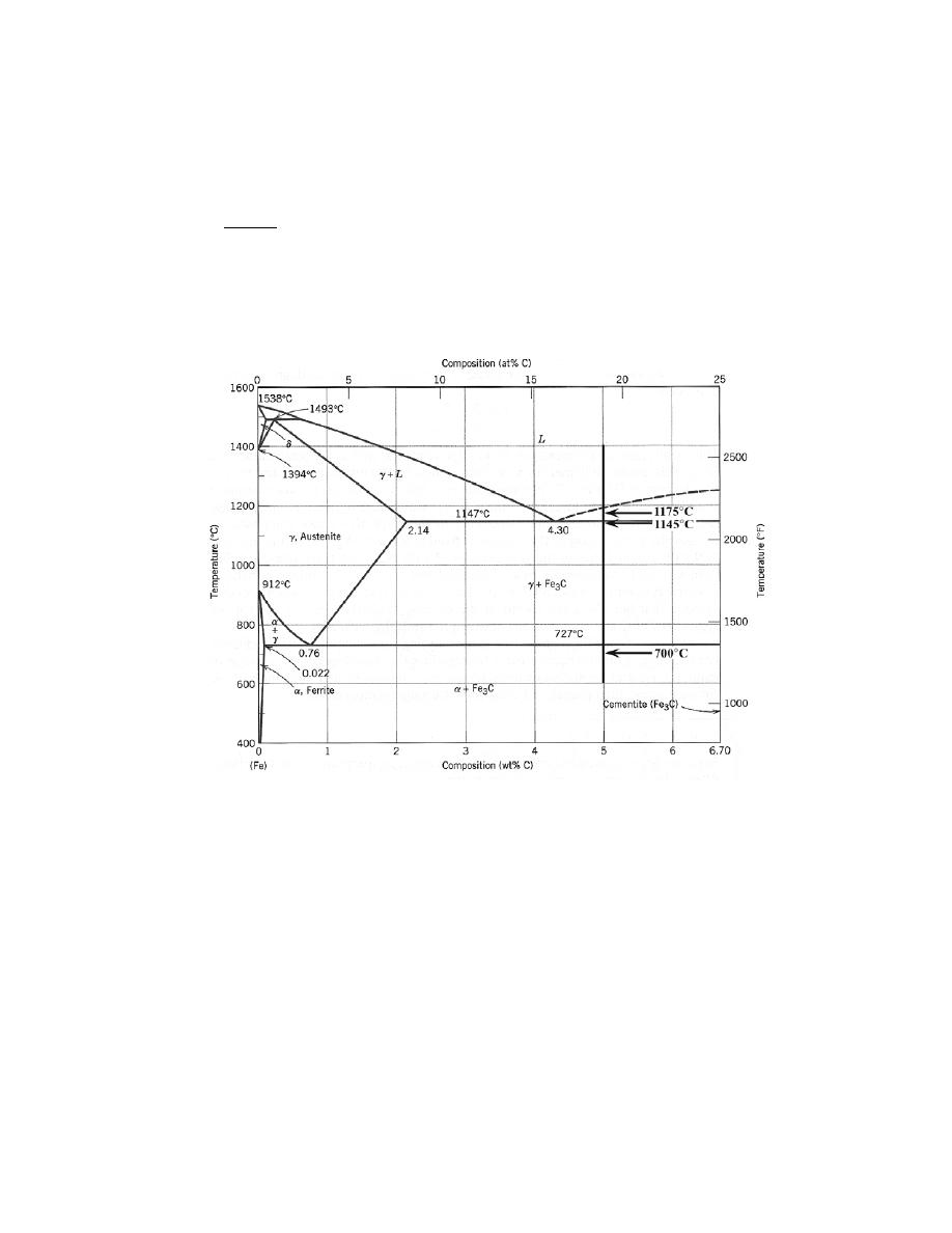
Excerpts from this work may be reproduced by instructors for distribution on a not-for-profit basis for testing or instructional purposes only to
students enrolled in courses for which the textbook has been adopted. Any other reproduction or translation of this work beyond that permitted
by Sections 107 or 108 of the 1976 United States Copyright Act without the permission of the copyright owner is unlawful.
9.63 For an iron-carbon alloy of composition 5 wt% C-95 wt% Fe, make schematic sketches of the
microstructure that would be observed for conditions of very slow cooling at the following temperatures: 1175
°C
(2150
°F), 1145°C (2095°F), and 700°C (1290°F). Label the phases and indicate their compositions (approximate).
Solution
Below is shown the Fe-Fe
3
C phase diagram (Figure 9.24). A vertical line at a composition of 5 wt% C-95
wt% Fe has been drawn, and, in addition, horizontal arrows at the three temperatures called for in the problem
statement (i.e., 1175
°C, 1145°C, and 700°C).
On the basis of the locations of the three temperature-composition points, schematic sketches of the
respective microstructures along with phase compositions are represented as follows:
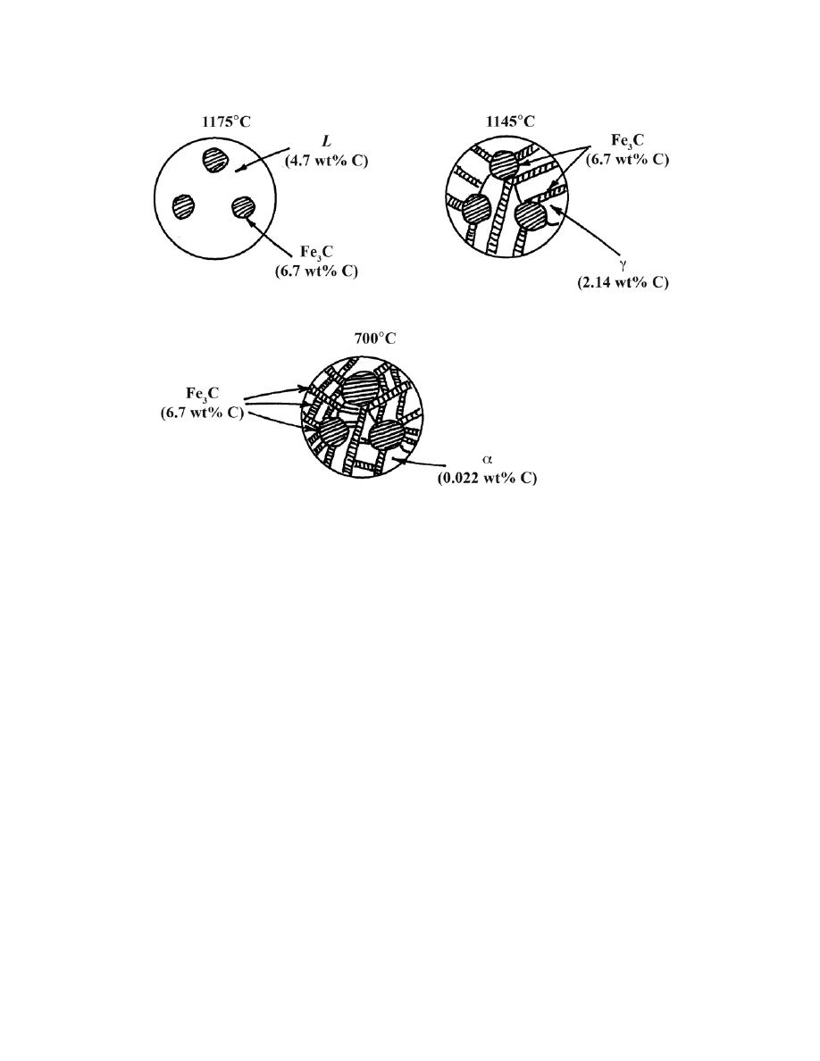
Excerpts from this work may be reproduced by instructors for distribution on a not-for-profit basis for testing or instructional purposes only to
students enrolled in courses for which the textbook has been adopted. Any other reproduction or translation of this work beyond that permitted
by Sections 107 or 108 of the 1976 United States Copyright Act without the permission of the copyright owner is unlawful.
9.64 Often, the properties of multiphase alloys may be approximated by the relationship
E (alloy) = E
α
V
α
+ E
β
V
β
(9.24)
where E represents a specific property (modulus of elasticity, hardness, etc.), and V is the volume fraction. The
subscripts α and β denote the existing phases or microconstituents. Employ the relationship above to determine the
approximate Brinell hardness of a 99.80 wt% Fe–0.20 wt% C alloy. Assume Brinell hardnesses of 80 and 280 for
ferrite and pearlite, respectively, and that volume fractions may be approximated by mass fractions.
Solution
This problem asks that we determine the approximate Brinell hardness of a 99.80 wt% Fe-0.20 wt% C
alloy, using a relationship similar to Equation 9.24. First, we compute the mass fractions of pearlite and
proeutectoid ferrite using Equations 9.20 and 9.21, as
W
p
=
C
0
'
− 0.022
0.74
=
0.20
− 0.022
0.74
= 0.24
W
α'
=
0.76
− C
0
'
0.74
=
0.76
− 0.20
0.74
= 0.76
Now, we compute the Brinell hardness of the alloy using a modified form of Equation 9.24 as
HB
alloy
= HB
α'
W
α'
+ HB
p
W
p
= (80)(0.76) + (280)(0.24) = 128

Excerpts from this work may be reproduced by instructors for distribution on a not-for-profit basis for testing or instructional purposes only to
students enrolled in courses for which the textbook has been adopted. Any other reproduction or translation of this work beyond that permitted
by Sections 107 or 108 of the 1976 United States Copyright Act without the permission of the copyright owner is unlawful.
The Influence of Other Alloying Elements
9.65 A steel alloy contains 97.5 wt% Fe, 2.0 wt% Mo, and 0.5 wt% C.
(a) What is the eutectoid temperature of this alloy?
(b) What is the eutectoid composition?
(c) What is the proeutectoid phase?
Assume that there are no changes in the positions of other phase boundaries with the addition of Mo.
Solution
(a) From Figure 9.34, the eutectoid temperature for 2.0 wt% Mo is approximately 850
°C.
(b) From Figure 9.35, the eutectoid composition is approximately 0.22 wt% C.
(c) Since the carbon concentration of the alloy (0.5 wt%) is greater than the eutectoid (0.22 wt% C),
cementite is the proeutectoid phase.
Excerpts from this work may be reproduced by instructors for distribution on a not-for-profit basis for testing or instructional purposes only to
students enrolled in courses for which the textbook has been adopted. Any other reproduction or translation of this work beyond that permitted
by Sections 107 or 108 of the 1976 United States Copyright Act without the permission of the copyright owner is unlawful.
9.66 A steel alloy is known to contain 93.8 wt% Fe, 6.0 wt% Ni, and 0.2 wt% C.
(a) What is the approximate eutectoid temperature of this alloy?
(b) What is the proeutectoid phase when this alloy is cooled to a temperature just below the eutectoid?
(c) Compute the relative amounts of the proeutectoid phase and pearlite.
Assume that there are no alterations in the positions of other phase boundaries with the addition of Ni.
Solution
(a) From Figure 9.34, the eutectoid temperature for 6.0 wt% Ni is approximately 650
°C (1200°F).
(b) From Figure 9.35, the eutectoid composition is approximately 0.62 wt% C. Since the carbon
concentration in the alloy (0.2 wt%) is less than the eutectoid (0.62 wt% C), the proeutectoid phase is ferrite.
(c) Assume that the
α–(α + Fe
3
C) phase boundary is at a negligible carbon concentration. Modifying
Equation 9.21 leads to
W
α'
=
0.62
− C
0
'
0.62
− 0
=
0.62
− 0.20
0.62
= 0.68
Likewise, using a modified Equation 9.20
W
p
=
C
0
'
− 0
0.62
− 0
=
0.20
0.62
= 0.32

Excerpts from this work may be reproduced by instructors for distribution on a not-for-profit basis for testing or instructional purposes only to
students enrolled in courses for which the textbook has been adopted. Any other reproduction or translation of this work beyond that permitted
by Sections 107 or 108 of the 1976 United States Copyright Act without the permission of the copyright owner is unlawful.
CHAPTER 10
PHASE TRANSFORMATIONS IN METALS
PROBLEM SOLUTIONS
The Kinetics of Phase Transformations
10.1 Name the two stages involved in the formation of particles of a new phase. Briefly describe each.
Solution
The two stages involved in the formation of particles of a new phase are nucleation and growth. The
nucleation process involves the formation of normally very small particles of the new phase(s) which are stable and
capable of continued growth. The growth stage is simply the increase in size of the new phase particles.

Excerpts from this work may be reproduced by instructors for distribution on a not-for-profit basis for testing or instructional purposes only to
students enrolled in courses for which the textbook has been adopted. Any other reproduction or translation of this work beyond that permitted
by Sections 107 or 108 of the 1976 United States Copyright Act without the permission of the copyright owner is unlawful.
10.2 (a) Rewrite the expression for the total free energy change for nucleation (Equation 10.1) for the case
of a cubic nucleus of edge length a (instead of a sphere of radius r). Now differentiate this expression with respect
to a (per Equation 10.2) and solve for both the critical cube edge length, a*
, and also ΔG*.
(b)
Is ΔG* greater for a cube or a sphere? Why?
Solution
(a) This problem first asks that we rewrite the expression for the total free energy change for nucleation
(analogous to Equation 10.1) for the case of a cubic nucleus of edge length a. The volume of such a cubic radius is
a
3
, whereas the total surface area is 6a
2
(since there are six faces each of which has an area of a
2
). Thus, the
expression for
∆G is as follows:
∆G = a
3
∆G
v
+ 6a
2
γ
Differentiation of this expression with respect to a is as
d
∆G
da
=
d
(
a
3
∆G
v
)
da
+
d
(
6a
2
γ
)
da
= 3a
2
∆G
v
+ 12a γ
If we set this expression equal to zero as
3a
2
∆G
v
+ 12a γ = 0
and then solve for a (= a*), we have
a * =
−
4
γ
∆G
v
Substitution of this expression for a in the above expression for
∆G yields an equation for ∆G* as
∆G * = (a*)
3
∆G
v
+ 6(a*)
2
γ
= −
4
γ
∆G
v
3
∆G
v
+ 6 γ −
4
γ
∆G
v
2

Excerpts from this work may be reproduced by instructors for distribution on a not-for-profit basis for testing or instructional purposes only to
students enrolled in courses for which the textbook has been adopted. Any other reproduction or translation of this work beyond that permitted
by Sections 107 or 108 of the 1976 United States Copyright Act without the permission of the copyright owner is unlawful.
=
32
γ
3
(
∆G
v
)
2
(b)
∆G
v
for a cube—i.e.,
(32)
γ
3
(
∆G
v
)
2
—is greater that for a sphere—i.e.,
16
π
3
γ
3
(
∆G
v
)
2
=
(16.8)
γ
3
(
∆G
v
)
2
. The reason for this is that surface-to-volume ratio of a cube is greater than for a sphere.

Excerpts from this work may be reproduced by instructors for distribution on a not-for-profit basis for testing or instructional purposes only to
students enrolled in courses for which the textbook has been adopted. Any other reproduction or translation of this work beyond that permitted
by Sections 107 or 108 of the 1976 United States Copyright Act without the permission of the copyright owner is unlawful.
10.3 If copper (which has a melting point of 1085°C) homogeneously nucleates at 849°C, calculate the
critical radius given values of –1.77 × 10
9
J/m
3
and 0.200 J/m
2
, respectively, for the latent heat of fusion and the
surface free energy.
Solution
This problem states that copper homogeneously nucleates at 849
°C, and that we are to calculate the critical
radius given the latent heat of fusion
(
–1.77
× 10
9
J/m
3
)
and the surface free energy
(
0.200 J/m
2
)
. Solution to this
problem requires the utilization of Equation 10.6 as
r *
= −
2
γT
m
∆H
f
1
T
m
− T
= −
(2)
(
0.200 J / m
2
)
(1085
+ 273 K)
−1.77 × 10
9
J / m
3
1
1085
°C − 849°C
= 1.30 × 10
−9
m
= 1.30 nm

Excerpts from this work may be reproduced by instructors for distribution on a not-for-profit basis for testing or instructional purposes only to
students enrolled in courses for which the textbook has been adopted. Any other reproduction or translation of this work beyond that permitted
by Sections 107 or 108 of the 1976 United States Copyright Act without the permission of the copyright owner is unlawful.
10.4
(a) For the solidification of iron, calculate the critical radius r* and the activation free energy ΔG* if
nucleation is homogeneous. Values for the latent heat of fusion and surface free energy are –1.85 × 10
9
J/m
3
and
0.204 J/m
2
, respectively. Use the supercooling value found in Table 10.1.
(b) Now calculate the number of atoms found in a nucleus of critical size. Assume a lattice parameter of
0.292 nm for solid iron at its melting temperature.
Solution
(a) This portion of the problem asks that we compute r* and
∆G* for the homogeneous nucleation of the
solidification of Fe. First of all, Equation 10.6 is used to compute the critical radius. The melting temperature for
iron, found inside the front cover is 1538
°C; also values of ∆H
f
(
–1.85
× 10
9
J/m
3
)
and
γ
(
0.204 J/m
2
)
are given in
the problem statement, and the supercooling value found in Table 10.1 is 295
°C (or 295 K). Thus, from Equation
10.6 we have
r *
= −
2
γT
m
∆H
f
1
T
m
− T
= −
(2)
(
0.204 J / m
2
)
(1538
+ 273 K)
−1.85 × 10
9
J / m
3
1
295 K
=
1.35
× 10
−9
m
= 1.35 nm
For computation of the activation free energy, Equation 10.7 is employed. Thus
∆G * =
16
π γ
3
T
m
2
3
∆H
f
2
1
(T
m
− T)
2
=
(16)(
π)
(
0.204 J / m
2
)
3
(1538
+ 273 K)
2
(3)
(
−1.85 × 10
9
J / m
3
)
2
1
(295 K)
2
= 1.57 × 10
−18
J
(b) In order to compute the number of atoms in a nucleus of critical size (assuming a spherical nucleus of
radius r*), it is first necessary to determine the number of unit cells, which we then multiply by the number of atoms
per unit cell. The number of unit cells found in this critical nucleus is just the ratio of critical nucleus and unit cell
volumes. Inasmuch as iron has the BCC crystal structure, its unit cell volume is just a
3
where a is the unit cell

Excerpts from this work may be reproduced by instructors for distribution on a not-for-profit basis for testing or instructional purposes only to
students enrolled in courses for which the textbook has been adopted. Any other reproduction or translation of this work beyond that permitted
by Sections 107 or 108 of the 1976 United States Copyright Act without the permission of the copyright owner is unlawful.
length (i.e., the lattice parameter); this value is 0.292 nm, as cited in the problem statement. Therefore, the number
of unit cells found in a radius of critical size is just
# unit cells / particle
=
4
3
πr
* 3
a
3
=
4
3
(
π)(1.35 nm)
3
(0.292 nm)
3
= 414 unit cells
Inasmuch as 2 atoms are associated with each BCC unit cell, the total number of atoms per critical nucleus is just
(414 unit cells / critical nucleus)(2 atoms / unit cell)
= 828 atoms /critical nucleus

Excerpts from this work may be reproduced by instructors for distribution on a not-for-profit basis for testing or instructional purposes only to
students enrolled in courses for which the textbook has been adopted. Any other reproduction or translation of this work beyond that permitted
by Sections 107 or 108 of the 1976 United States Copyright Act without the permission of the copyright owner is unlawful.
10.5 (a) Assume for the solidification of iron (Problem 10.4) that nucleation is homogeneous, and the
number of stable nuclei is 10
6
nuclei per cubic meter. Calculate the critical radius and the number of stable nuclei
that exist at the following degrees of supercooling: 200 K and 300 K.
(b) What is significant about the magnitudes of these critical radii and the numbers of stable nuclei?
Solution
(a) For this part of the problem we are asked to calculate the critical radius for the solidification of iron
(per Problem 10.4), for 200 K and 300 K degrees of supercooling, and assuming that the there are 10
6
nuclei per
meter cubed for homogeneous nucleation. In order to calculate the critical radii, we replace the T
m
– T term in
Equation 10.6 by the degree of supercooling (denoted as
∆T) cited in the problem.
For 200 K supercooling,
r
200
*
= −
2
γT
m
∆H
f
1
∆T
= −
(2)
(
0.204 J / m
2
)
(1538
+ 273 K)
−1.85 × 10
9
J / m
3
1
200 K
= 2.00
× 10
-9
m = 2.00 nm
And, for 300 K supercooling,
r
300
* = −
(2)
(
0.204 J / m
2
)
(1538
+ 273 K)
−1.85 × 10
9
J / m
3
1
300 K
= 1.33
× 10
-9
m = 1.33 nm
In order to compute the number of stable nuclei that exist at 200 K and 300 K degrees of supercooling, it
is necessary to use Equation 10.8. However, we must first determine the value of K
1
in Equation 10.8, which in turn
requires that we calculate
∆G* at the homogeneous nucleation temperature using Equation 10.7; this was done in
Problem 10.4, and yielded a value of
∆G* = 1.57 × 10
-18
J. Now for the computation of K
1
, using the value of n*
for at the homogenous nucleation temperature
(
10
6
nuclei/m3
)
:
K
1
=
n *
exp
−
∆G *
kT

Excerpts from this work may be reproduced by instructors for distribution on a not-for-profit basis for testing or instructional purposes only to
students enrolled in courses for which the textbook has been adopted. Any other reproduction or translation of this work beyond that permitted
by Sections 107 or 108 of the 1976 United States Copyright Act without the permission of the copyright owner is unlawful.
=
10
6
nuclei / m
3
exp
−
1.57
× 10
−18
J
(
1.38
× 10
−23
J / atom
− K
)
(1538
°C − 295°C)
= 5.62
× 10
45
nuclei/m
3
Now for 200 K supercooling, it is first necessary to recalculate the value
∆G* of using Equation 10.7, where, again,
the T
m
– T term is replaced by the number of degrees of supercooling, denoted as
∆T, which in this case is 200 K.
Thus
∆G
200
*
=
16
π γ
3
T
m
2
3
∆H
f
2
1
(
∆T)
2
=
(16)(
π)
(
0.204 J / m
2
)
3
(1538
+ 273 K)
2
(3)
(
−1.85 × 10
9
J / m
3
)
2
1
(200 K)
2
= 3.41
× 10
-18
J
And, from Equation 10.8, the value of n* is
n
200
*
= K
1
exp
−
∆G
200
*
kT
=
(
5.62
× 10
45
nuclei / m
3
)
exp
−
3.41
× 10
−18
J
(
1.38
× 10
−23
J / atom
− K
)
(1538 K
− 200 K)
= 3.5
× 10
-35
stable nuclei
Now, for 300 K supercooling the value of
∆G* is equal to
∆G
300
*
=
(16)(
π)
(
0.204 J / m
2
)
3
(1538
+ 273 K)
2
(3)
(
−1.85 × 10
9
J / m
3
)
2
1
(300 K)
2
= 1.51
× 10
-18
J

Excerpts from this work may be reproduced by instructors for distribution on a not-for-profit basis for testing or instructional purposes only to
students enrolled in courses for which the textbook has been adopted. Any other reproduction or translation of this work beyond that permitted
by Sections 107 or 108 of the 1976 United States Copyright Act without the permission of the copyright owner is unlawful.
from which we compute the number of stable nuclei at 300 K of supercooling as
n
300
*
= K
1
exp
−
∆G
300
*
kT
n*
=
(
5.62
× 10
45
nuclei / m
3
)
exp
−
1.51
× 10
−18
J
(
1.38
× 10
−23
J / atom
− K
)
(1538 K
− 300 K)
= 2.32
× 10
7
stable nuclei
(b) Relative to critical radius, r* for 300 K supercooling is slightly smaller that for 200 K (1.33 nm versus
2.00 nm). [From Problem 10.4, the value of r* at the homogeneous nucleation temperature (295 K) was 1.35 nm.]
More significant, however, are the values of n* at these two degrees of supercooling, which are dramatically
different—3.5
× 10
-35
stable nuclei at
∆T = 200 K, versus 2.32 × 10
7
stable nuclei at
∆T = 300 K!

Excerpts from this work may be reproduced by instructors for distribution on a not-for-profit basis for testing or instructional purposes only to
students enrolled in courses for which the textbook has been adopted. Any other reproduction or translation of this work beyond that permitted
by Sections 107 or 108 of the 1976 United States Copyright Act without the permission of the copyright owner is unlawful.
10.6 For some transformation having kinetics that obey the Avrami equation (Equation 10.17), the
parameter n is known to have a value of 1.7. If, after 100 s, the reaction is 50% complete, how long (total time) will
it take the transformation to go to 99% completion?
Solution
This problem calls for us to compute the length of time required for a reaction to go to 99% completion. It
first becomes necessary to solve for the parameter k in Equation 10.17. In order to do this it is best manipulate the
equation such that k is the dependent variable. We first rearrange Equation 10.17 as
exp
(
− kt
n
)
= 1 − y
and then take natural logarithms of both sides:
− kt
n
= ln(1 − y)
Now solving for k gives
k =
−
ln (1
− y)
t
n
And, from the problem statement, for y = 0.50 when t = 100 s and given that n = 1.7, the value of k is equal to
k =
−
ln (1
− 0.5)
(100 s)
1.7
= 2.76
× 10
-4
We now want to manipulate Equation 10.17 such that t is the dependent variable. The above equation may be
written in the form:
t
n
=
−
ln (1
− y)
k
And solving this expression for t leads to
t =
−
ln (1
− y)
k
1/n

Excerpts from this work may be reproduced by instructors for distribution on a not-for-profit basis for testing or instructional purposes only to
students enrolled in courses for which the textbook has been adopted. Any other reproduction or translation of this work beyond that permitted
by Sections 107 or 108 of the 1976 United States Copyright Act without the permission of the copyright owner is unlawful.
Now, using this equation and the value of k determined above, the time to 99% transformation completion is equal
to
t =
−
ln (1
− 0.99)
2.76
× 10
−4
1/1.7
= 305 s

Excerpts from this work may be reproduced by instructors for distribution on a not-for-profit basis for testing or instructional purposes only to
students enrolled in courses for which the textbook has been adopted. Any other reproduction or translation of this work beyond that permitted
by Sections 107 or 108 of the 1976 United States Copyright Act without the permission of the copyright owner is unlawful.
10.7 Compute the rate of some reaction that obeys Avrami kinetics, assuming that the constants n and k
have values of 3.0 and 7
× 10
-3
, respectively, for time expressed in seconds.
Solution
This problem asks that we compute the rate of some reaction given the values of n and k in Equation 10.17.
Since the reaction rate is defined by Equation 10.18, it is first necessary to determine t
0.5
, or the time necessary for
the reaction to reach y = 0.5. We must first manipulate Equation 10.17 such that t is the dependent variable. We
first rearrange Equation 10.17 as
exp
(
− kt
n
)
= 1 −
y
and then take natural logarithms of both sides:
− kt
n
= ln (1 − y)
which my be rearranged so as to read
t
n
=
−
ln (1
− y)
k
Now, solving for t from this expression leads to
t =
−
ln (1
− y)
k
1/n
For t
0.5
this equation takes the form
t
0.5
=
−
ln (1
− 0.5)
k
1/ n
And, incorporation of values for n and k given in the problem statement (3.0 and 7
× 10
-3
, respectively), then
t
0.5
=
−
ln (1
− 0.5)
7
× 10
−3
1/3.0
= 4.63 s
Now, the rate is computed using Equation 10.18 as

Excerpts from this work may be reproduced by instructors for distribution on a not-for-profit basis for testing or instructional purposes only to
students enrolled in courses for which the textbook has been adopted. Any other reproduction or translation of this work beyond that permitted
by Sections 107 or 108 of the 1976 United States Copyright Act without the permission of the copyright owner is unlawful.
rate =
1
t
0.5
=
1
4.63 s
= 0.216 s
-1

Excerpts from this work may be reproduced by instructors for distribution on a not-for-profit basis for testing or instructional purposes only to
students enrolled in courses for which the textbook has been adopted. Any other reproduction or translation of this work beyond that permitted
by Sections 107 or 108 of the 1976 United States Copyright Act without the permission of the copyright owner is unlawful.
10.8 It is known that the kinetics of recrystallization for some alloy obey the Avrami equation and that the
value of n in the exponential is 2.5. If, at some temperature, the fraction recrystallized is 0.40 after 200 min,
determine the rate of recrystallization at this temperature.
Solution
This problem gives us the value of y (0.40) at some time t (200 min), and also the value of n (2.5) for the
recrystallization of an alloy at some temperature, and then asks that we determine the rate of recrystallization at this
same temperature. It is first necessary to calculate the value of k. We first rearrange Equation 10.17 as
exp
(
− kt
n
)
= 1 −
y
and then take natural logarithms of both sides:
− kt
n
= ln (1 − y)
Now solving for k gives
k =
−
ln (1
− y)
t
n
which, using the values cited above for y, n, and t yields
k =
−
ln (1
− 0.40)
(200 min)
2.5
= 9.0
× 10
-7
At this point we want to compute t
0.5
, the value of t for y = 0.5, which means that it is necessary to establish a form
of Equation 10.17 in which t is the dependent variable. From one of the above equations
t
n
=
−
ln (1
− y)
k
And solving this expression for t leads to
t =
−
ln (1
− y)
k
1/n

Excerpts from this work may be reproduced by instructors for distribution on a not-for-profit basis for testing or instructional purposes only to
students enrolled in courses for which the textbook has been adopted. Any other reproduction or translation of this work beyond that permitted
by Sections 107 or 108 of the 1976 United States Copyright Act without the permission of the copyright owner is unlawful.
For t
0.5
, this equation takes the form
t
0.5
=
−
ln (1
− 0.5)
k
1/ n
and incorporation of the value of k determined above, as well as the value of n cited in the problem statement (2.5),
then t
0.5
is equal to
t
0.5
=
−
ln (1
− 0.5)
9.0
× 10
−7
1/2.5
= 226.3 min
Therefore, from Equation 10.18, the rate is just
rate =
1
t
0.5
=
1
226.3 min
= 4.42
× 10
-3
(min)
-1

Excerpts from this work may be reproduced by instructors for distribution on a not-for-profit basis for testing or instructional purposes only to
students enrolled in courses for which the textbook has been adopted. Any other reproduction or translation of this work beyond that permitted
by Sections 107 or 108 of the 1976 United States Copyright Act without the permission of the copyright owner is unlawful.
10.9 The kinetics of the austenite-to-pearlite transformation obey the Avrami relationship. Using the
fraction transformed–time data given here, determine the total time required for 95% of the austenite to transform
to pearlite:
Fraction Transformed
Time (s)
0.2
12.6
0.8
28.2
Solution
The first thing necessary is to set up two expressions of the form of Equation 10.17, and then to solve
simultaneously for the values of n and k. In order to expedite this process, we will rearrange and do some algebraic
manipulation of Equation 10.17. First of all, we rearrange as follows:
1
− y = exp − kt
n
( )
Now taking natural logarithms
ln (1
− y) = − kt
n
Or
− ln (1 − y) = kt
n
which may also be expressed as
ln
1
1
− y
= kt
n
Now taking natural logarithms again, leads to
ln ln
1
1
− y
= ln k + n ln t

Excerpts from this work may be reproduced by instructors for distribution on a not-for-profit basis for testing or instructional purposes only to
students enrolled in courses for which the textbook has been adopted. Any other reproduction or translation of this work beyond that permitted
by Sections 107 or 108 of the 1976 United States Copyright Act without the permission of the copyright owner is unlawful.
which is the form of the equation that we will now use. Using values cited in the problem statement, the two
equations are thus
ln
ln
1
1
− 0.2
= ln k + n ln (12.6 s)
ln
ln
1
1
− 0.8
= ln k + n ln (28.2 s)
Solving these two expressions simultaneously for n and k yields n = 2.453 and k = 4.46
× 10
-4
.
Now it becomes necessary to solve for the value of t at which y = 0.95. One of the above equations—viz
− ln (1 − y) = kt
n
may be rewritten as
t
n
=
−
ln (1
− y)
k
And solving for t leads to
t =
−
ln (1
− y)
k
1/n
Now incorporating into this expression values for n and k determined above, the time required for 95% austenite
transformation is equal to
t =
−
ln (1
− 0.95)
4.64
× 10
−4
1/2.453
= 35.7 s

Excerpts from this work may be reproduced by instructors for distribution on a not-for-profit basis for testing or instructional purposes only to
students enrolled in courses for which the textbook has been adopted. Any other reproduction or translation of this work beyond that permitted
by Sections 107 or 108 of the 1976 United States Copyright Act without the permission of the copyright owner is unlawful.
10.10 The fraction recrystallized–time data for the recrystallization at 600°C of a previously deformed
steel are tabulated here. Assuming that the kinetics of this process obey the Avrami relationship, determine the
fraction recrystallized after a total time of 22.8 min.
Fraction
Recrystallized
Time (min)
0.20
13.1
0.70
29.1
Solution
The first thing necessary is to set up two expressions of the form of Equation 10.17, and then to solve
simultaneously for the values of n and k. In order to expedite this process, we will rearrange and do some algebraic
manipulation of Equation 10.17. First of all, we rearrange as follows:
1
− y = exp − kt
n
( )
Now taking natural logarithms
ln (1
− y) = − kt
n
Or
− ln (1 − y) = kt
n
which may also be expressed as
ln
1
1
− y
= kt
n
Now taking natural logarithms again, leads to
ln ln
1
1
− y
= ln k + n ln t
which is the form of the equation that we will now use. The two equations are thus

Excerpts from this work may be reproduced by instructors for distribution on a not-for-profit basis for testing or instructional purposes only to
students enrolled in courses for which the textbook has been adopted. Any other reproduction or translation of this work beyond that permitted
by Sections 107 or 108 of the 1976 United States Copyright Act without the permission of the copyright owner is unlawful.
ln
ln
1
1
− 0.20
= ln k + n ln (13.1 min)
ln
ln
1
1
− 0.70
= ln k + n ln (29.1 min)
Solving these two expressions simultaneously for n and k yields n = 2.112 and k = 9.75
× 10
-4
.
Now it becomes necessary to solve for y when t = 22.8 min. Application of Equation 10.17 leads to
y = 1
− exp −kt
n
( )
= 1
− exp −
(
9.75
× 10
-4
)
(
22.8 min
)
2.112
[
]
= 0.51
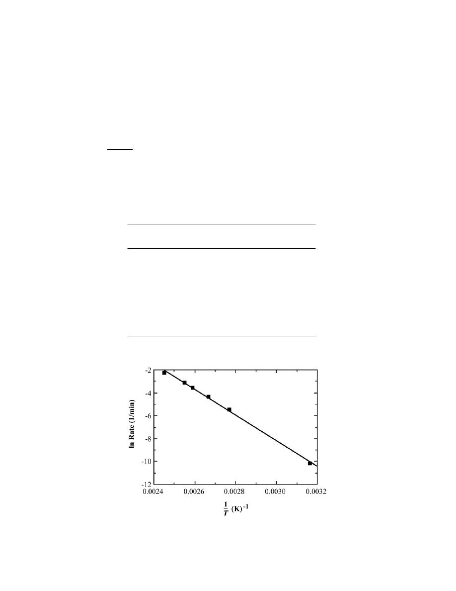
Excerpts from this work may be reproduced by instructors for distribution on a not-for-profit basis for testing or instructional purposes only to
students enrolled in courses for which the textbook has been adopted. Any other reproduction or translation of this work beyond that permitted
by Sections 107 or 108 of the 1976 United States Copyright Act without the permission of the copyright owner is unlawful.
10.11 (a) From the curves shown in Figure 10.11 and using Equation 10.18, determine the rate of
recrystallization for pure copper at the several temperatures.
(b) Make a plot of ln(rate) versus the reciprocal of temperature (in K
–1
), and determine the activation
energy for this recrystallization process. (See Section 5.5.)
(c) By extrapolation, estimate the length of time required for 50% recrystallization at room temperature,
20°C (293 K).
Solution
This problem asks us to consider the percent recrystallized versus logarithm of time curves for copper
shown in Figure 10.11.
(a) The rates at the different temperatures are determined using Equation 10.18, which rates are tabulated
below:
Temperature (
°C)
Rate (min)
-1
135
0.105
119
4.4
× 10
-2
113
2.9
× 10
-2
102
1.25
× 10
-2
88
4.2
× 10
-3
43
3.8
× 10
-5
(b) These data are plotted below.

Excerpts from this work may be reproduced by instructors for distribution on a not-for-profit basis for testing or instructional purposes only to
students enrolled in courses for which the textbook has been adopted. Any other reproduction or translation of this work beyond that permitted
by Sections 107 or 108 of the 1976 United States Copyright Act without the permission of the copyright owner is unlawful.
The activation energy, Q, is related to the slope of the line drawn through the data points as
Q =
− Slope (R)
where R is the gas constant. The slope of this line is equal to
Slope
=
∆ ln rate
∆
1
T
=
ln rate
1
− ln rate
2
1
T
1
−
1
T
2
Let us take 1/T
1
= 0.0025 K
-1
and 1/T
2
= 0.0031 K
-1
; the corresponding ln rate values are ln rate
1
= -2.6 and ln
rate
2
= -9.4. Thus, using these values, the slope is equal to
Slope
=
−2.6 − (−9.4)
0.0025 K
-1
− 0.0031 K
-1
= −1.133 × 10
4
K
And, finally the activation energy is
Q =
− (Slope)(R) = −
(
−1.133 × 10
4
K
-1
)
(8.31 J/mol - K)
= 94,150 J/mol
(c) At room temperature (20
°C), 1/T = 1/(20 + 273 K) = 3.41 × 10
-3
K
-1
. Extrapolation of the data in the
plot to this 1/T value gives
ln (rate)
≅ −12.8
which leads to
rate
≅ exp (−12.8) = 2.76 × 10
-6
(min)
-1
But since
rate =
1
t
0.5

Excerpts from this work may be reproduced by instructors for distribution on a not-for-profit basis for testing or instructional purposes only to
students enrolled in courses for which the textbook has been adopted. Any other reproduction or translation of this work beyond that permitted
by Sections 107 or 108 of the 1976 United States Copyright Act without the permission of the copyright owner is unlawful.
t
0.5
=
1
rate
=
1
2.76
× 10
−6
(min)
−1
= 3.62 × 10
5
min
= 250 days

Excerpts from this work may be reproduced by instructors for distribution on a not-for-profit basis for testing or instructional purposes only to
students enrolled in courses for which the textbook has been adopted. Any other reproduction or translation of this work beyond that permitted
by Sections 107 or 108 of the 1976 United States Copyright Act without the permission of the copyright owner is unlawful.
10.12 Determine values for the constants n and k (Equation 10.17) for the recrystallization of copper
(Figure 10.11) at 102°C.
Solution
In this problem we are asked to determine, from Figure 10.11, the values of the constants n and k (Equation
10.17) for the recrystallization of copper at 102
°C. One way to solve this problem is to take two values of percent
recrystallization (which is just 100y, Equation 10.17) and their corresponding time values, then set up two
simultaneous equations, from which n and k may be determined. In order to expedite this process, we will rearrange
and do some algebraic manipulation of Equation 10.17. First of all, we rearrange as follows:
1
− y = exp − kt
n
( )
Now taking natural logarithms
ln (1
− y) = − kt
n
Or
− ln (1 − y) = kt
n
which may also be expressed as
ln
1
1
− y
= kt
n
Now taking natural logarithms again, leads to
ln ln
1
1
− y
= ln k + n ln t
which is the form of the equation that we will now use. From the 102
°C curve of Figure 10.11, let us arbitrarily
choose two percent recrystallized values, 20% and 80% (i.e., y
1
= 0.20 and y
2
= 0.80). Their corresponding time
values are t
1
= 50 min and t
2
= 100 min (realizing that the time axis is scaled logarithmically). Thus, our two
simultaneous equations become

Excerpts from this work may be reproduced by instructors for distribution on a not-for-profit basis for testing or instructional purposes only to
students enrolled in courses for which the textbook has been adopted. Any other reproduction or translation of this work beyond that permitted
by Sections 107 or 108 of the 1976 United States Copyright Act without the permission of the copyright owner is unlawful.
ln ln
1
1
− 0.2
= ln k + n ln (50)
ln ln
1
1
− 0.8
= ln k + n ln (100)
from which we obtain the values n = 2.85 and k = 3.21
× 10
-6
.

Excerpts from this work may be reproduced by instructors for distribution on a not-for-profit basis for testing or instructional purposes only to
students enrolled in courses for which the textbook has been adopted. Any other reproduction or translation of this work beyond that permitted
by Sections 107 or 108 of the 1976 United States Copyright Act without the permission of the copyright owner is unlawful.
Metastable Versus Equilibrium States
10.13 In terms of heat treatment and the development of microstructure, what are two major limitations of
the iron–iron carbide phase diagram?
Solution
Two limitations of the iron-iron carbide phase diagram are:
(1) The nonequilibrium martensite does not appear on the diagram; and
(2) The diagram provides no indication as to the time-temperature relationships for the formation of
pearlite, bainite, and spheroidite, all of which are composed of the equilibrium ferrite and cementite phases.

Excerpts from this work may be reproduced by instructors for distribution on a not-for-profit basis for testing or instructional purposes only to
students enrolled in courses for which the textbook has been adopted. Any other reproduction or translation of this work beyond that permitted
by Sections 107 or 108 of the 1976 United States Copyright Act without the permission of the copyright owner is unlawful.
10.14 (a) Briefly describe the phenomena of superheating and supercooling.
(b) Why do these phenomena occur?
Solution
(a) Superheating and supercooling correspond, respectively, to heating or cooling above or below a phase
transition temperature without the occurrence of the transformation.
(b) These phenomena occur because right at the phase transition temperature, the driving force is not
sufficient to cause the transformation to occur. The driving force is enhanced during superheating or supercooling.

Excerpts from this work may be reproduced by instructors for distribution on a not-for-profit basis for testing or instructional purposes only to
students enrolled in courses for which the textbook has been adopted. Any other reproduction or translation of this work beyond that permitted
by Sections 107 or 108 of the 1976 United States Copyright Act without the permission of the copyright owner is unlawful.
Isothermal Transformation Diagrams
10.15 Suppose that a steel of eutectoid composition is cooled to 550°C (1020°F) from 760°C (1400°F) in
less than 0.5 s and held at this temperature.
(a) How long will it take for the austenite-to-pearlite reaction to go to 50% completion? To 100%
completion?
(b) Estimate the hardness of the alloy that has completely transformed to pearlite.
Solution
We are called upon to consider the isothermal transformation of an iron-carbon alloy of eutectoid
composition.
(a) From Figure 10.22, a horizontal line at 550
°C intersects the 50% and reaction completion curves at
about 2.5 and 6 seconds, respectively; these are the times asked for in the problem statement.
(b) The pearlite formed will be fine pearlite. From Figure 10.30a, the hardness of an alloy of composition
0.76 wt% C that consists of fine pearlite is about 265 HB (27 HRC).

Excerpts from this work may be reproduced by instructors for distribution on a not-for-profit basis for testing or instructional purposes only to
students enrolled in courses for which the textbook has been adopted. Any other reproduction or translation of this work beyond that permitted
by Sections 107 or 108 of the 1976 United States Copyright Act without the permission of the copyright owner is unlawful.
10.16 Briefly cite the differences between pearlite, bainite, and spheroidite relative to microstructure and
mechanical properties.
Solution
The microstructures of pearlite, bainite, and spheroidite all consist of
α-ferrite and cementite phases. For
pearlite, the two phases exist as layers which alternate with one another. Bainite consists of very fine and parallel
needle-shaped particles of cementite that are surrounded an
α-ferrite matrix. For spheroidite, the matrix is ferrite,
and the cementite phase is in the shape of sphere-shaped particles.
Bainite is harder and stronger than pearlite, which, in turn, is harder and stronger than spheroidite.

Excerpts from this work may be reproduced by instructors for distribution on a not-for-profit basis for testing or instructional purposes only to
students enrolled in courses for which the textbook has been adopted. Any other reproduction or translation of this work beyond that permitted
by Sections 107 or 108 of the 1976 United States Copyright Act without the permission of the copyright owner is unlawful.
10.17 What is the driving force for the formation of spheroidite?
Solution
The driving force for the formation of spheroidite is the net reduction in ferrite-cementite phase boundary
area.
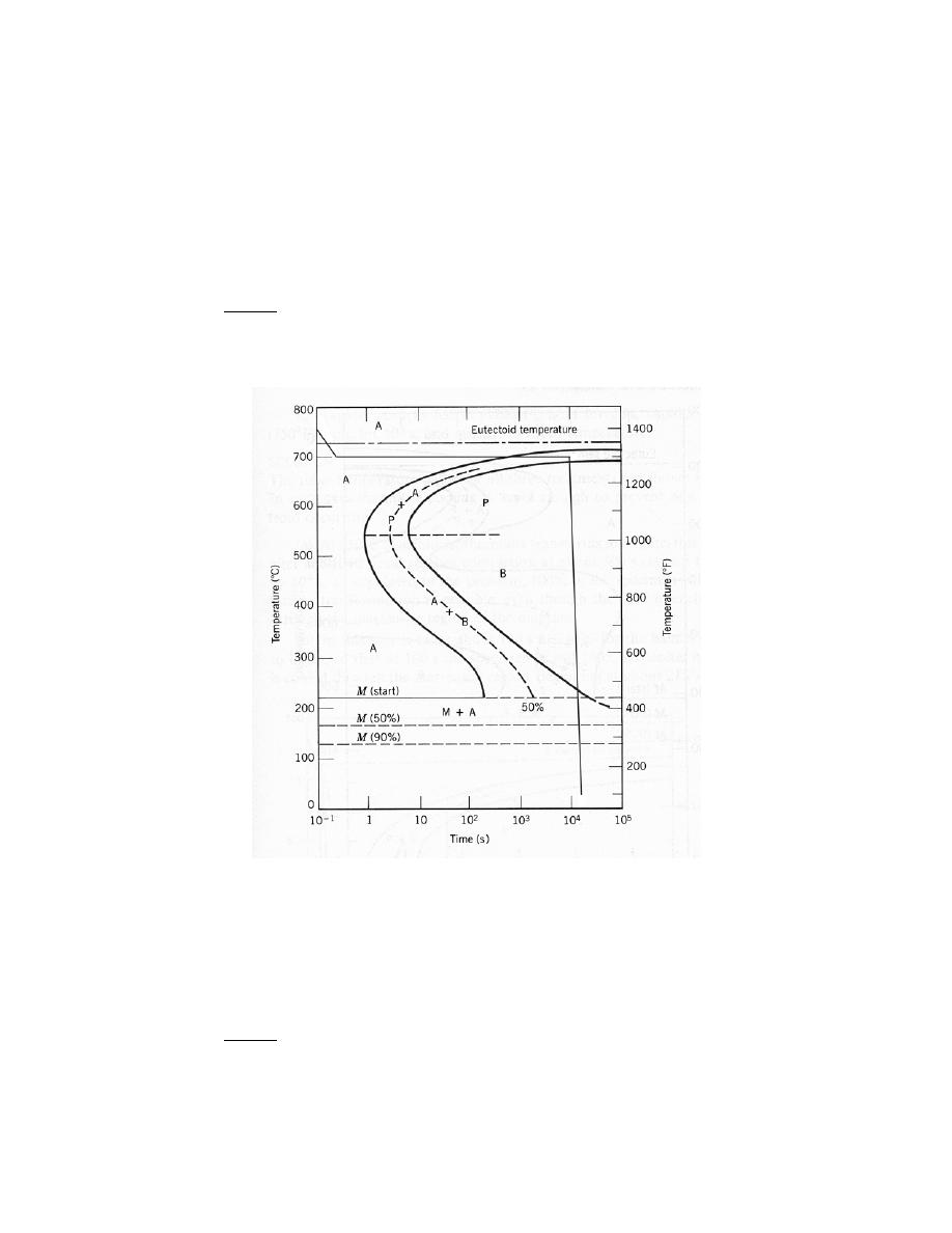
Excerpts from this work may be reproduced by instructors for distribution on a not-for-profit basis for testing or instructional purposes only to
students enrolled in courses for which the textbook has been adopted. Any other reproduction or translation of this work beyond that permitted
by Sections 107 or 108 of the 1976 United States Copyright Act without the permission of the copyright owner is unlawful.
10.18 Using the isothermal transformation diagram for an iron–carbon alloy of eutectoid composition
(Figure 10.22), specify the nature of the final microstructure (in terms of microconstituents present and
approximate percentages of each) of a small specimen that has been subjected to the following time–temperature
treatments. In each case assume that the specimen begins at 760°C (1400°F) and that it has been held at this
temperature long enough to have achieved a complete and homogeneous austenitic structure.
(a) Cool rapidly to 700°C (1290°F), hold for 10
4
s, then quench to room temperature.
Solution
Below is Figure 10.22 upon which is superimposed the above heat treatment.
After cooling and holding at 700°C for 10
4
s, approximately 50% of the specimen has transformed to
coarse pearlite. Upon cooling to room temperature, the remaining 50% transforms to martensite. Hence, the final
microstructure consists of about 50% coarse pearlite and 50% martensite.
(b) Reheat the specimen in part (a) to 700°C (1290°F) for 20 h.
Solution
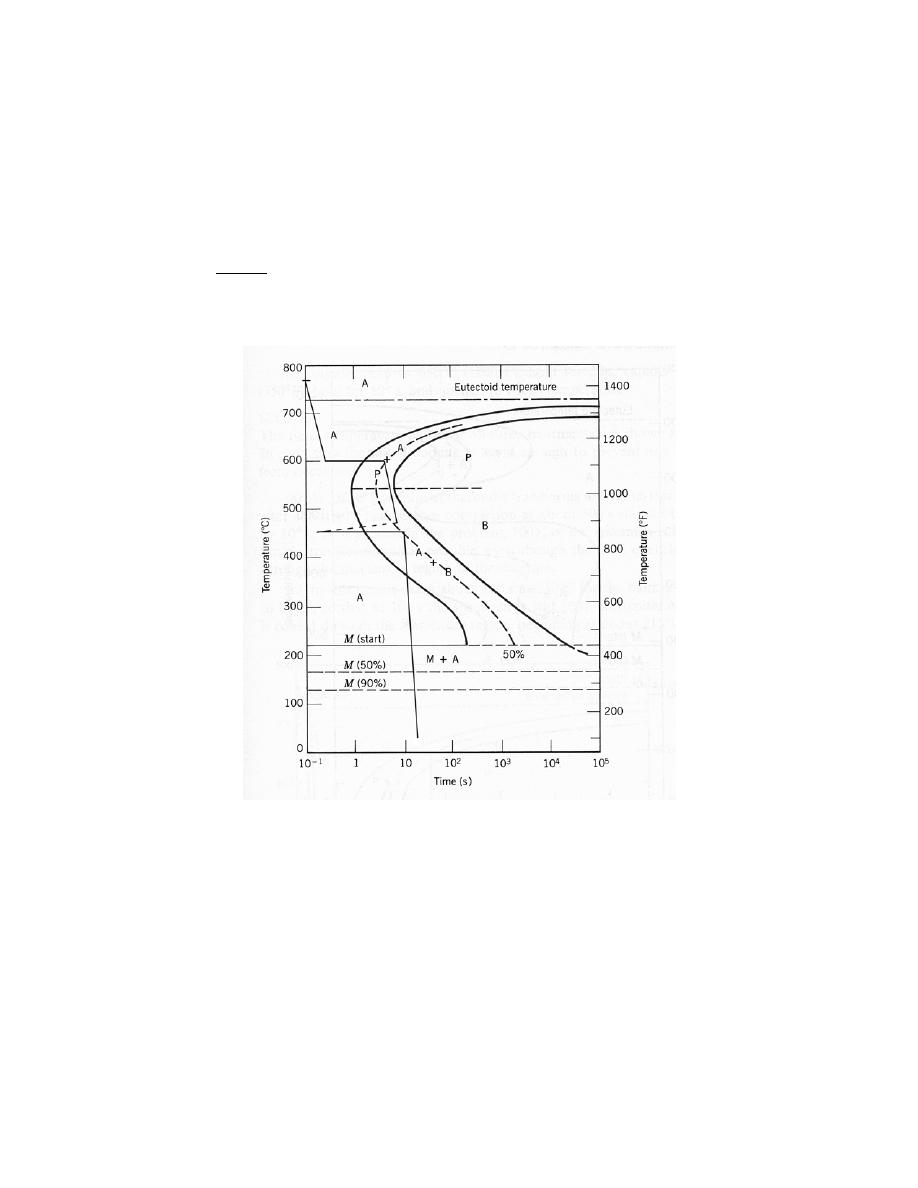
Excerpts from this work may be reproduced by instructors for distribution on a not-for-profit basis for testing or instructional purposes only to
students enrolled in courses for which the textbook has been adopted. Any other reproduction or translation of this work beyond that permitted
by Sections 107 or 108 of the 1976 United States Copyright Act without the permission of the copyright owner is unlawful.
Heating to 700°C for 20 h the specimen in part (a) will transform the coarse pearlite and martensite to
spheroidite.
(c) Rapidly cool to 600°C (1110°F), hold for 4 s, rapidly cool to 450°C (840°F), hold for 10 s, then quench
to room temperature.
Solution
Below is Figure 10.22 upon which is superimposed the above heat treatment.
After cooling to and holding at 600°C for 4 s, approximately 50% of the specimen has transformed to
pearlite (medium). During the rapid cooling to 450°C no transformations occur. At 450°C we start timing again at
zero time; while holding at 450°C for 10 s, approximately 50 percent of the remaining unreacted 50% (or 25% of
the original specimen) will transform to bainite. And upon cooling to room temperature, the remaining 25% of the
original specimen transforms to martensite. Hence, the final microstructure consists of about 50% pearlite
(medium), 25% bainite, and 25% martensite.
(d) Cool rapidly to 400°C (750°F), hold for 2 s, then quench to room temperature.
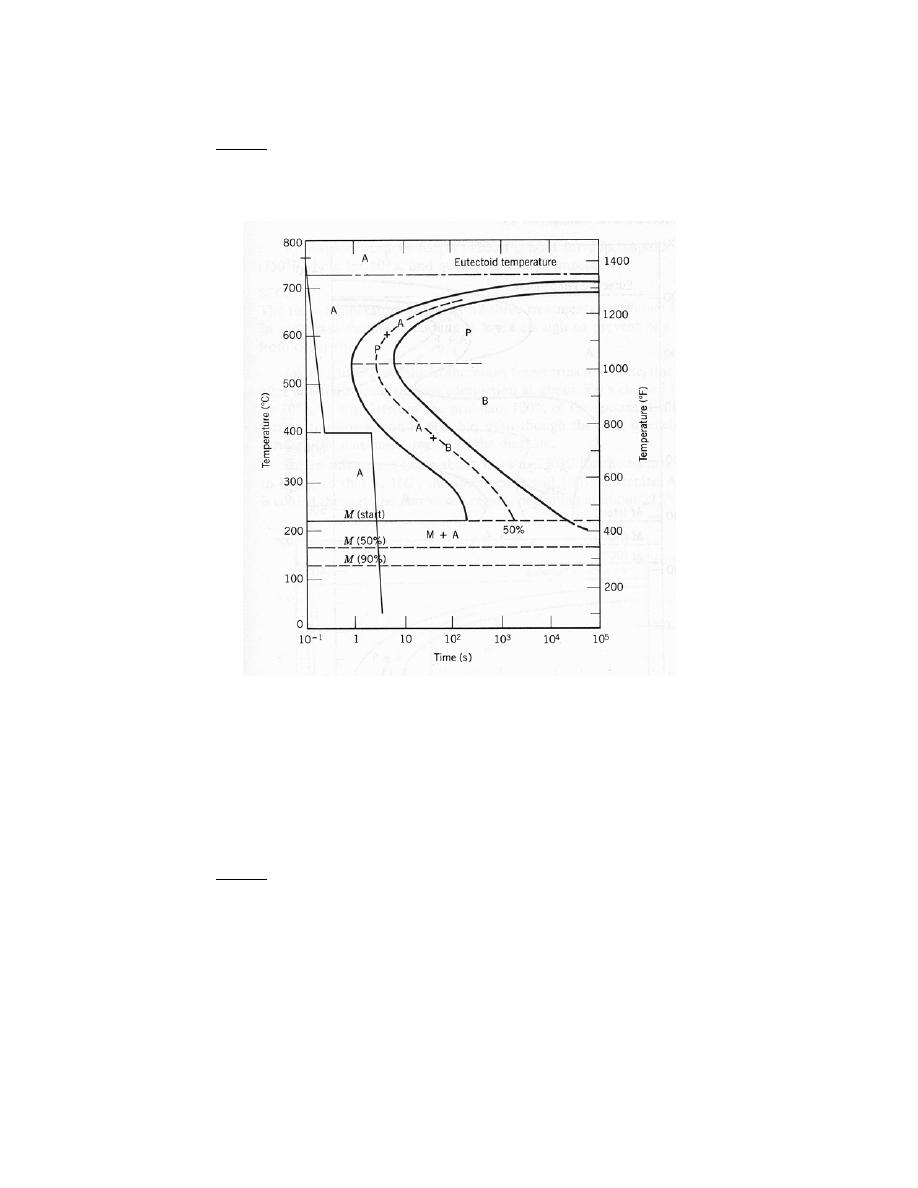
Excerpts from this work may be reproduced by instructors for distribution on a not-for-profit basis for testing or instructional purposes only to
students enrolled in courses for which the textbook has been adopted. Any other reproduction or translation of this work beyond that permitted
by Sections 107 or 108 of the 1976 United States Copyright Act without the permission of the copyright owner is unlawful.
Solution
Below is Figure 10.22 upon which is superimposed the above heat treatment.
After cooling to and holding at 400°C for 2 s, no of the transformation begin lines have been crossed, and
therefore, the specimen is 100% austenite. Upon cooling rapidly to room temperature, all of the specimen
transforms to martensite, such that the final microstructure is 100% martensite.
(e) Cool rapidly to 400°C (750°F), hold for 20 s, then quench to room temperature.
Solution
Below is Figure 10.22 upon which is superimposed the above heat treatment.
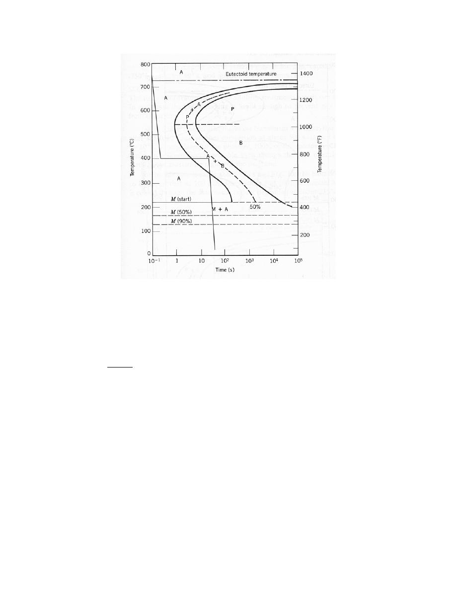
Excerpts from this work may be reproduced by instructors for distribution on a not-for-profit basis for testing or instructional purposes only to
students enrolled in courses for which the textbook has been adopted. Any other reproduction or translation of this work beyond that permitted
by Sections 107 or 108 of the 1976 United States Copyright Act without the permission of the copyright owner is unlawful.
After cooling and holding at 400°C for 20 s, approximately 40% of the specimen has transformed to
bainite. Upon cooling to room temperature, the remaining 60% transforms to martensite. Hence, the final
microstructure consists of about 40% bainite and 60% martensite.
(f) Cool rapidly to 400°C (750°F), hold for 200 s, then quench to room temperature.
Solution
Below is Figure 10.22 upon which is superimposed the above heat treatment.
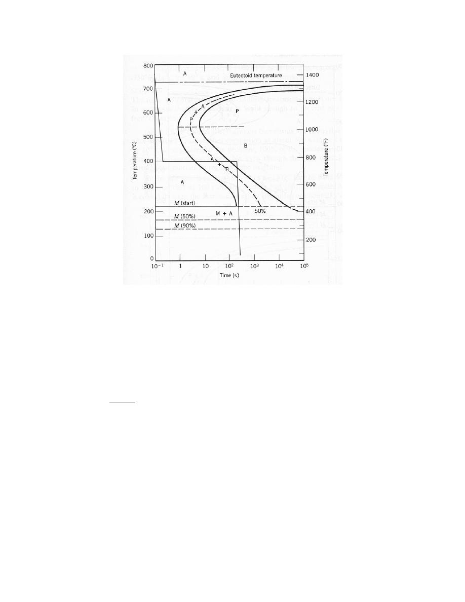
Excerpts from this work may be reproduced by instructors for distribution on a not-for-profit basis for testing or instructional purposes only to
students enrolled in courses for which the textbook has been adopted. Any other reproduction or translation of this work beyond that permitted
by Sections 107 or 108 of the 1976 United States Copyright Act without the permission of the copyright owner is unlawful.
After cooling and holding at 400°C for 200 s, the entire specimen has transformed to bainite. Therefore,
during the cooling to room temperature no additional transformations will occur. Hence, the final microstructure
consists of 100% bainite.
(g) Rapidly cool to 575°C (1065°F), hold for 20 s, rapidly cool to 350°C (660°F), hold for 100 s, then
quench to room temperature.
Solution
Below is Figure 10.22 upon which is superimposed the above heat treatment.
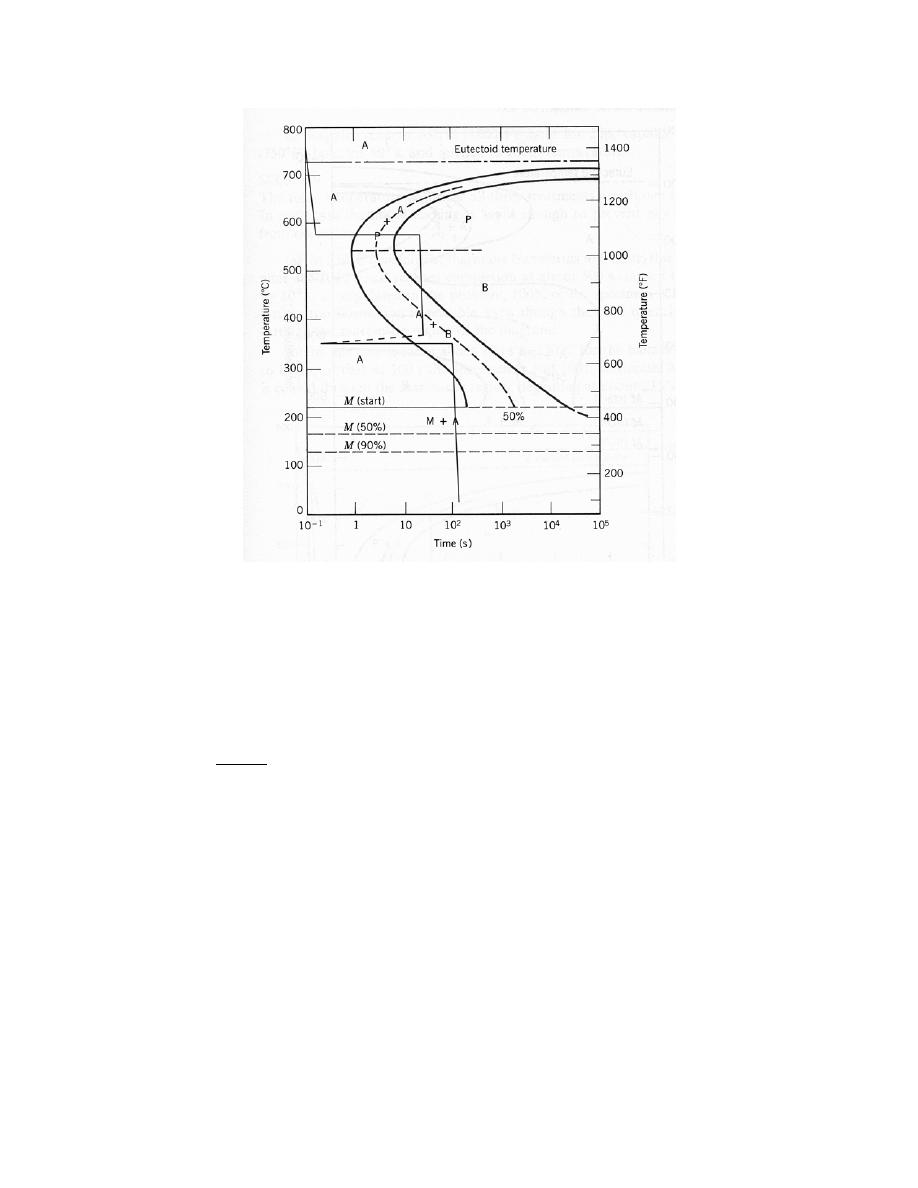
Excerpts from this work may be reproduced by instructors for distribution on a not-for-profit basis for testing or instructional purposes only to
students enrolled in courses for which the textbook has been adopted. Any other reproduction or translation of this work beyond that permitted
by Sections 107 or 108 of the 1976 United States Copyright Act without the permission of the copyright owner is unlawful.
After cooling and holding at 575°C for 20 s, the entire specimen has transformed to fine pearlite.
Therefore, during the second heat treatment at 350°C no additional transformations will occur. Hence, the final
microstructure consists of 100% fine pearlite.
(h) Rapidly cool to 250°C (480°F), hold for 100 s, then quench to room temperature in water. Reheat to
315°C (600°F) for 1 h and slowly cool to room temperature.
Solution
Below is Figure 10.22 upon which is superimposed the above heat treatment.
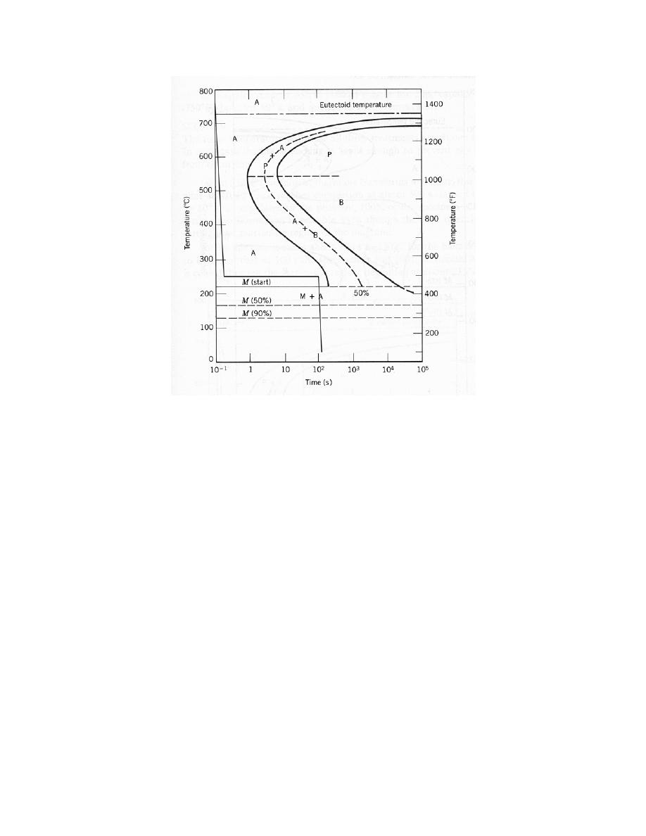
Excerpts from this work may be reproduced by instructors for distribution on a not-for-profit basis for testing or instructional purposes only to
students enrolled in courses for which the textbook has been adopted. Any other reproduction or translation of this work beyond that permitted
by Sections 107 or 108 of the 1976 United States Copyright Act without the permission of the copyright owner is unlawful.
After cooling and holding at 250°C for 100 s, no transformations will have occurred—at this point, the
entire specimen is still austenite. Upon rapidly cooling to room temperature in water, the specimen will completely
transform to martensite. The second heat treatment (at 315°C for 1 h)—not shown on the above plot—will
transform the material to tempered martensite. Hence, the final microstructure is 100% tempered martensite.
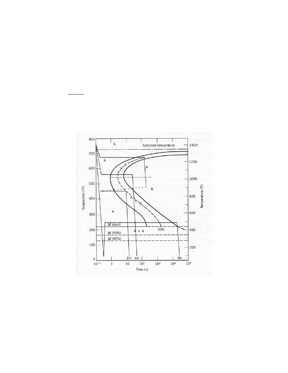
Excerpts from this work may be reproduced by instructors for distribution on a not-for-profit basis for testing or instructional purposes only to
students enrolled in courses for which the textbook has been adopted. Any other reproduction or translation of this work beyond that permitted
by Sections 107 or 108 of the 1976 United States Copyright Act without the permission of the copyright owner is unlawful.
10.19 Make a copy of the isothermal transformation diagram for an iron–carbon alloy of eutectoid
composition (Figure 10.22) and then sketch and label time–temperature paths on this diagram to produce the
following microstructures:
(a) 100% fine pearlite
(b) 100% tempered martensite
(c) 50% coarse pearlite, 25% bainite, and 25% martensite
Solution
Below is shown the isothermal transformation diagram for a eutectoid iron-carbon alloy, with time-
temperature paths that will yield (a) 100% fine pearlite; (b) 100% tempered martensite; and (c) 50% coarse
pearlite, 25% bainite, and 25% martensite.
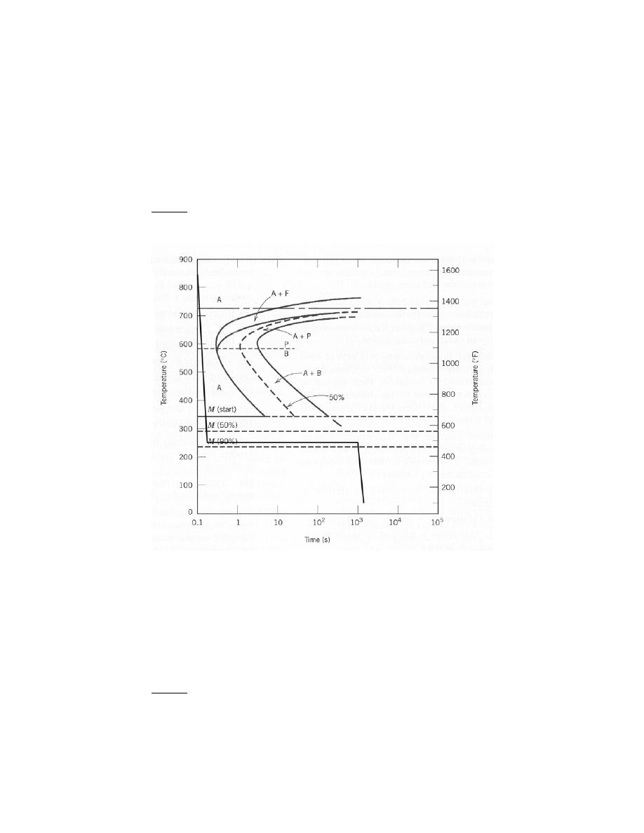
Excerpts from this work may be reproduced by instructors for distribution on a not-for-profit basis for testing or instructional purposes only to
students enrolled in courses for which the textbook has been adopted. Any other reproduction or translation of this work beyond that permitted
by Sections 107 or 108 of the 1976 United States Copyright Act without the permission of the copyright owner is unlawful.
10.20 Using the isothermal transformation diagram for a 0.45 wt% C steel alloy (Figure 10.39),
determine the final microstructure (in terms of just the microconstituents present) of a small specimen that has been
subjected to the following time-temperature treatments. In each case assume that the specimen begins at 845
°C
(1550
°F), and that it has been held at this temperature long enough to have achieved a complete and homogeneous
austenitic structure.
(a) Rapidly cool to 250
°C (480°F), hold for 10
3
s, then quench to room temperature.
Solution
Below is Figure 10.39 upon which is superimposed the above heat treatment.
While rapidly cooling to 250°C about 80% of the specimen transforms to martensite; during the 1000 s
isothermal treatment at 250°C no additional transformations occur. During the final cooling to room temperature,
the untransformed austenite also transforms to martensite. Hence, the final microstructure consists of 100%
martensite.
(b) Rapidly cool to 700
°C (1290°F), hold for 30 s, then quench to room temperature.
Solution
Below is Figure 10.39 upon which is superimposed the above heat treatment.
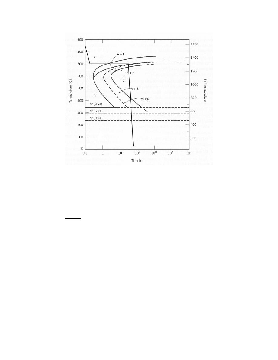
Excerpts from this work may be reproduced by instructors for distribution on a not-for-profit basis for testing or instructional purposes only to
students enrolled in courses for which the textbook has been adopted. Any other reproduction or translation of this work beyond that permitted
by Sections 107 or 108 of the 1976 United States Copyright Act without the permission of the copyright owner is unlawful.
After cooling to and holding at 700°C for 30 s, a portion of specimen has transformed to proeutectoid
ferrite. While cooling to room temperature, the remainder of the specimen transforms to martensite. Hence, the final
microstructure consists proeutectoid ferrite and martensite.
(c) Rapidly cool to 400
°C (750°F), hold for 500 s, then quench to room temperature.
Solution
Below is Figure 10.39 upon which is superimposed the above heat treatment.
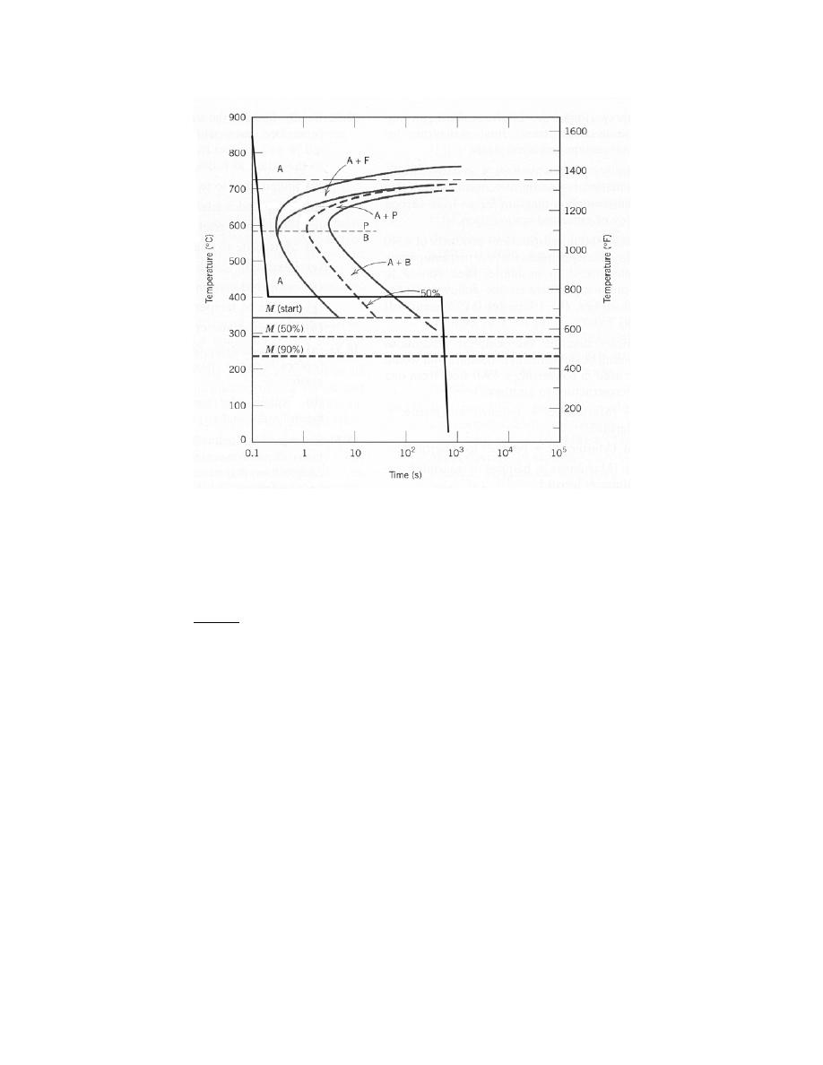
Excerpts from this work may be reproduced by instructors for distribution on a not-for-profit basis for testing or instructional purposes only to
students enrolled in courses for which the textbook has been adopted. Any other reproduction or translation of this work beyond that permitted
by Sections 107 or 108 of the 1976 United States Copyright Act without the permission of the copyright owner is unlawful.
After cooling to and holding at 400°C for 500 s, all of the specimen has transformed to bainite. Hence, the
final microstructure consists of 100% bainite.
(d) Rapidly cool to 700
°C (1290°F), hold at this temperature for 10
5
s, then quench to room temperature.
Solution
Below is Figure 10.39 upon which is superimposed the above heat treatment.
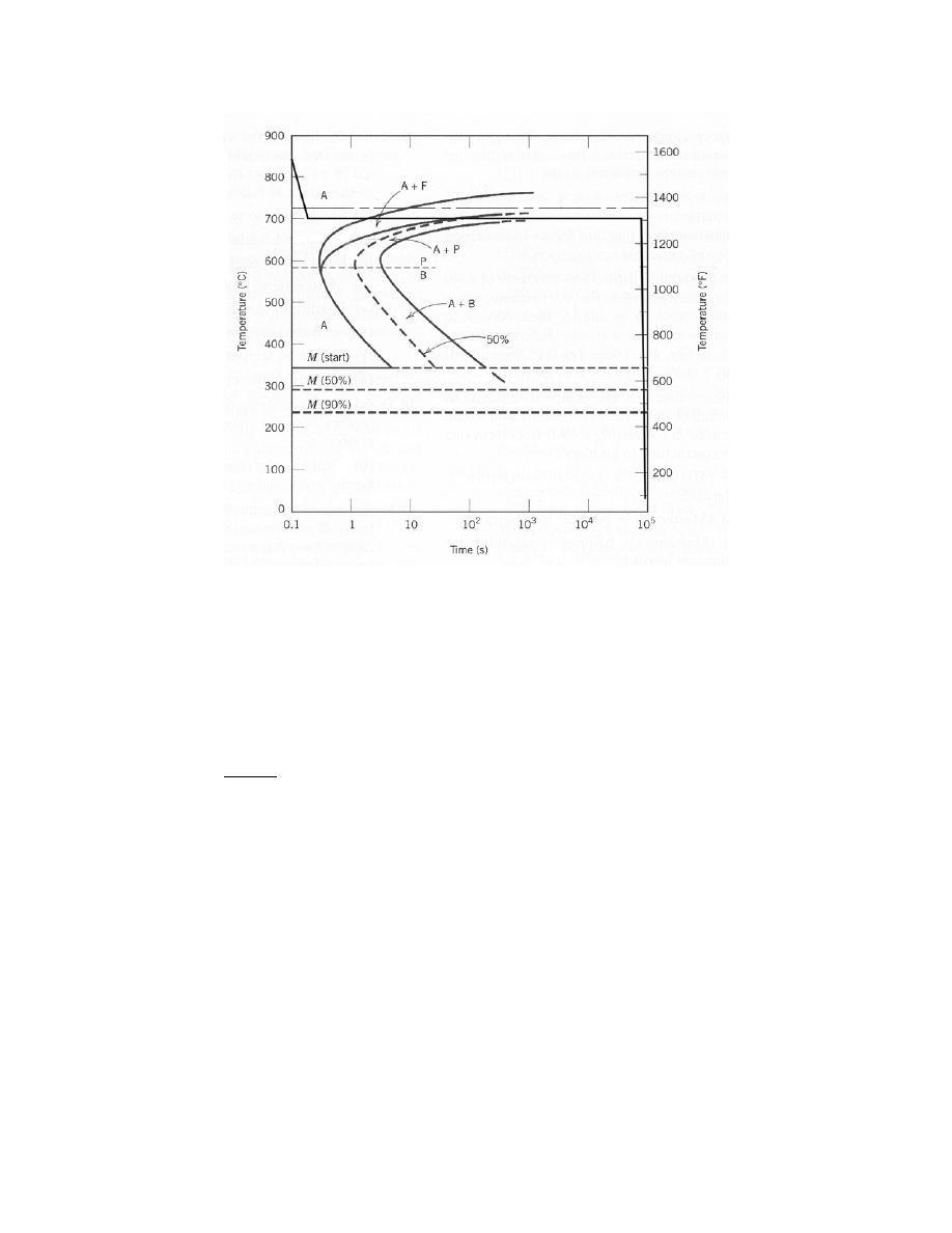
Excerpts from this work may be reproduced by instructors for distribution on a not-for-profit basis for testing or instructional purposes only to
students enrolled in courses for which the textbook has been adopted. Any other reproduction or translation of this work beyond that permitted
by Sections 107 or 108 of the 1976 United States Copyright Act without the permission of the copyright owner is unlawful.
After cooling to and while holding at 700°C the specimen first transforms to proeutectoid ferrite and coarse
pearlite. Continued heat treating at 700°C for 10
5
s results in a further transformation into spheroidite. Hence, the
final microstructure consists of 100% spheroidite.
(e) Rapidly cool to 650
°C (1200°F), hold at this temperature for 3 s, rapidly cool to 400°C (750°F), hold
for 10 s, then quench to room temperature.
Solution
Below is Figure 10.39 upon which is superimposed the above heat treatment.
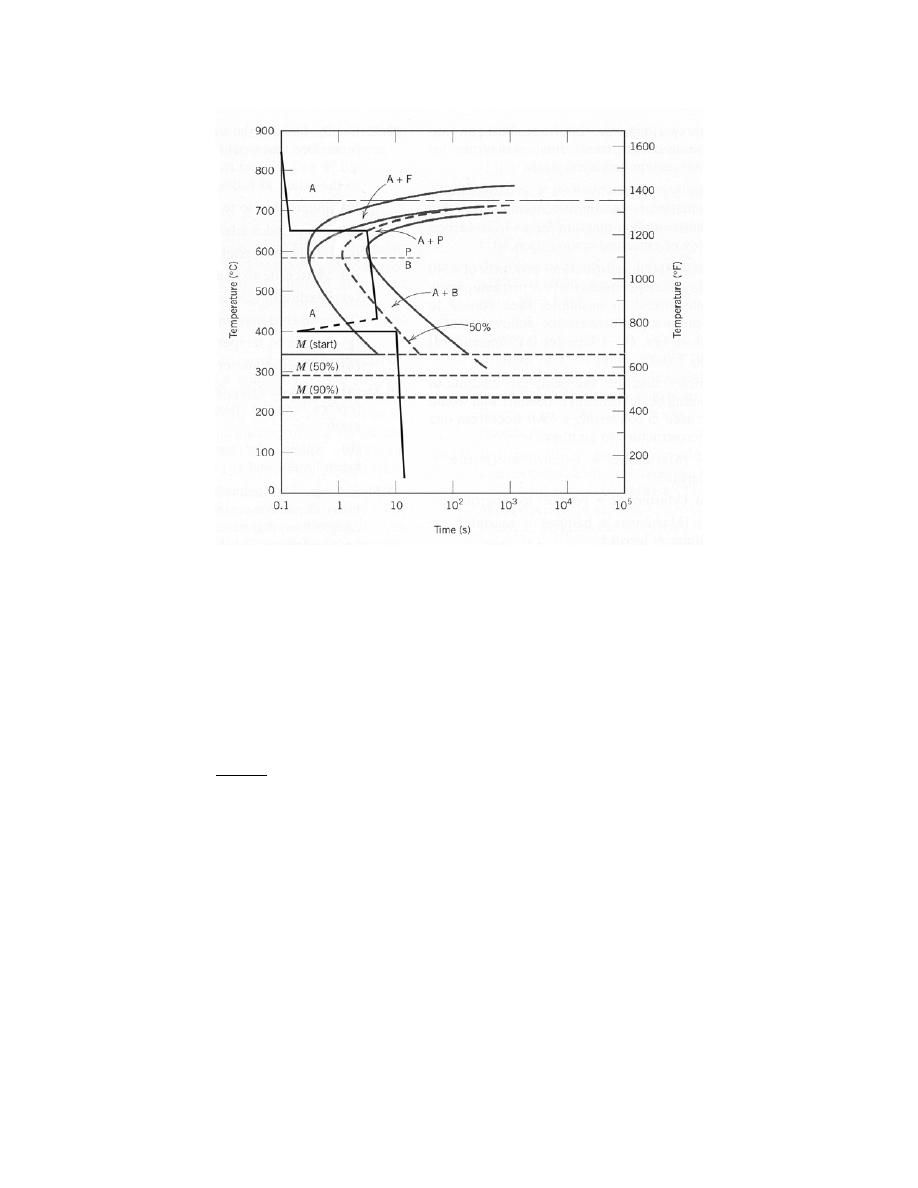
Excerpts from this work may be reproduced by instructors for distribution on a not-for-profit basis for testing or instructional purposes only to
students enrolled in courses for which the textbook has been adopted. Any other reproduction or translation of this work beyond that permitted
by Sections 107 or 108 of the 1976 United States Copyright Act without the permission of the copyright owner is unlawful.
After cooling to and holding at 650°C for 3 s, some of the specimen first transformers to proeutectoid
ferrite and then to pearlite (medium). During the second stage of the heat treatment at 400°C, some (but not all) of
the remaining unreacted austenite transforms to bainite. As a result of the final quenching, all of the remaining
austenite transforms to martensite. Hence, the final microstructure consists of ferrite, pearlite (medium), bainite,
and martensite.
(f) Rapidly cool to 450
°C (840°F), hold for 10 s, then quench to room temperature.
Solution
Below is Figure 10.39 upon which is superimposed the above heat treatment.
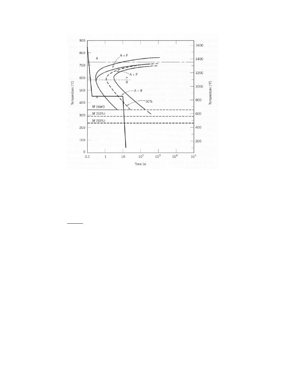
Excerpts from this work may be reproduced by instructors for distribution on a not-for-profit basis for testing or instructional purposes only to
students enrolled in courses for which the textbook has been adopted. Any other reproduction or translation of this work beyond that permitted
by Sections 107 or 108 of the 1976 United States Copyright Act without the permission of the copyright owner is unlawful.
After cooling to and holding at 450°C for 10 s, a portion of the specimen first transformers to bainite.
During the quenching to room temperature, the remainder of the specimen transforms to martensite. Hence, the final
microstructure consists of bainite and martensite.
(g) Rapidly cool to 625
°C (1155°F), hold for 1 s, then quench to room temperature.
Solution
Below is Figure 10.39 upon which is superimposed the above heat treatment.
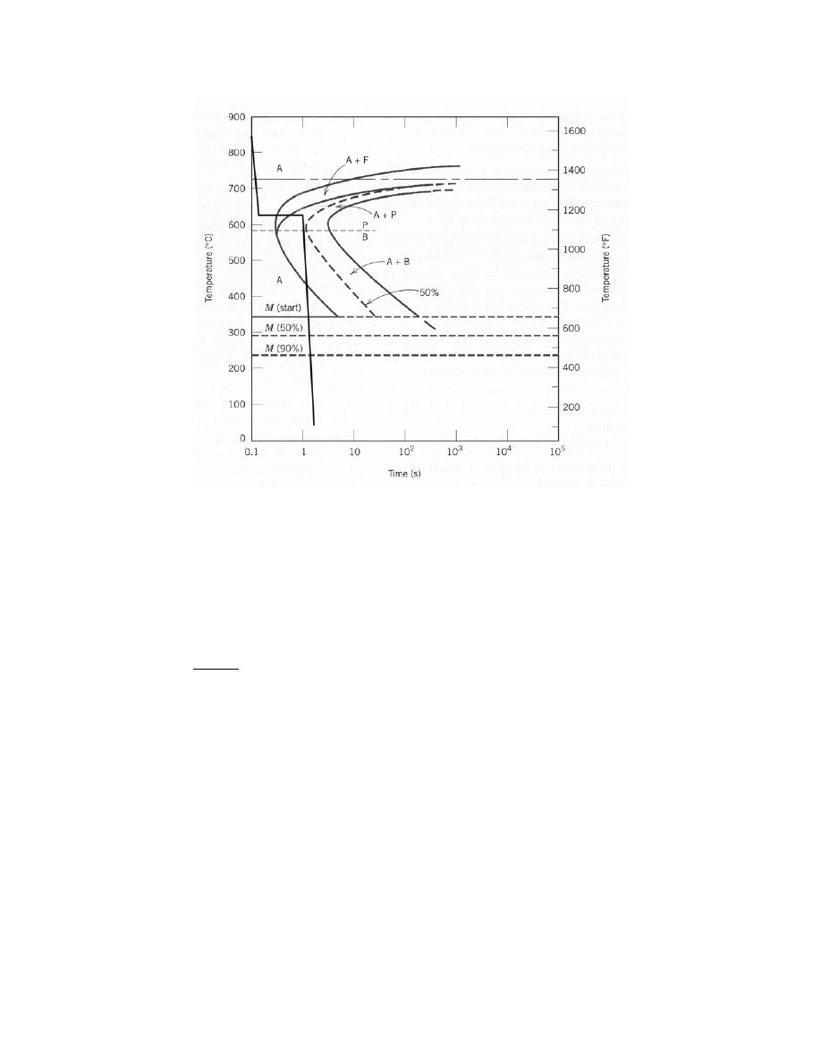
Excerpts from this work may be reproduced by instructors for distribution on a not-for-profit basis for testing or instructional purposes only to
students enrolled in courses for which the textbook has been adopted. Any other reproduction or translation of this work beyond that permitted
by Sections 107 or 108 of the 1976 United States Copyright Act without the permission of the copyright owner is unlawful.
After cooling to and holding at 625°C for 1 s, a portion of the specimen first transformers to proeutectoid
ferrite and pearlite. During the quenching to room temperature, the remainder of the specimen transforms to
martensite. Hence, the final microstructure consists of ferrite, pearlite, and martensite.
(h) Rapidly cool to 625
°C (1155°F), hold at this temperature for 10 s, rapidly cool to 400°C (750°F), hold
at this temperature for 5 s, then quench to room temperature.
Solution
Below is Figure 10.39 upon which is superimposed the above heat treatment.
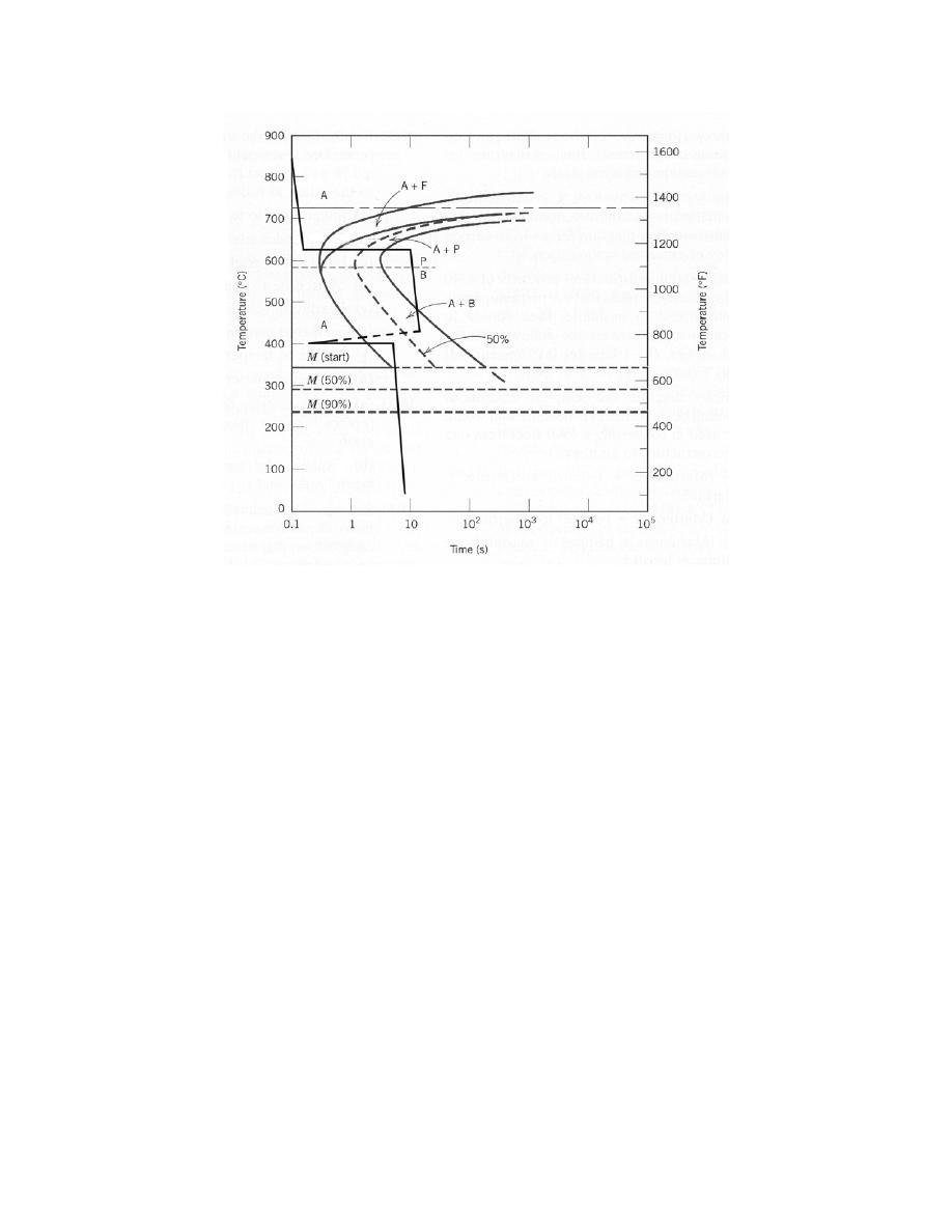
Excerpts from this work may be reproduced by instructors for distribution on a not-for-profit basis for testing or instructional purposes only to
students enrolled in courses for which the textbook has been adopted. Any other reproduction or translation of this work beyond that permitted
by Sections 107 or 108 of the 1976 United States Copyright Act without the permission of the copyright owner is unlawful.
After cooling to and holding at 625°C for 10 s, all of the specimen transformers to proeutectoid ferrite and
pearlite. During the second part of the heat treatment at 400°C no additional transformation will occur. Hence, the
final microstructure consists of ferrite and pearlite.
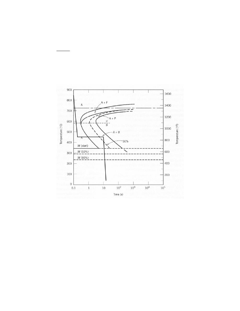
Excerpts from this work may be reproduced by instructors for distribution on a not-for-profit basis for testing or instructional purposes only to
students enrolled in courses for which the textbook has been adopted. Any other reproduction or translation of this work beyond that permitted
by Sections 107 or 108 of the 1976 United States Copyright Act without the permission of the copyright owner is unlawful.
10.21 For parts (a), (c), (d), (f), and (h) of Problem 10.20, determine the approximate percentages of the
microconstituents that form.
Solution
(a) From Problem 10.20(a) the microstructure consists of 100% martensite.
(c) From Problem 10.20(c) the microstructure consists of 100% bainite.
(d) From Problem 10.20(d) the microstructure consists of 100% spheroidite.
(f) Figure 10.39 onto which the heat treatment for Problem 10.20(f) has been constructed is shown below.
From this diagram, for the isothermal heat treatment at 450
°C, the horizontal line constructed at this temperature
and that ends at the 10 s point spans approximately 70% of the distance between the bainite reaction start and
reaction completion curves. Therefore, the final microstructure consists of about 70% bainite and 30% martensite
(the martensite forms while cooling to room temperature after 10 s at 450
°C).
(h) Figure 10.39 onto which the heat treatment for Problem 10.20(h) has been constructed is shown below.
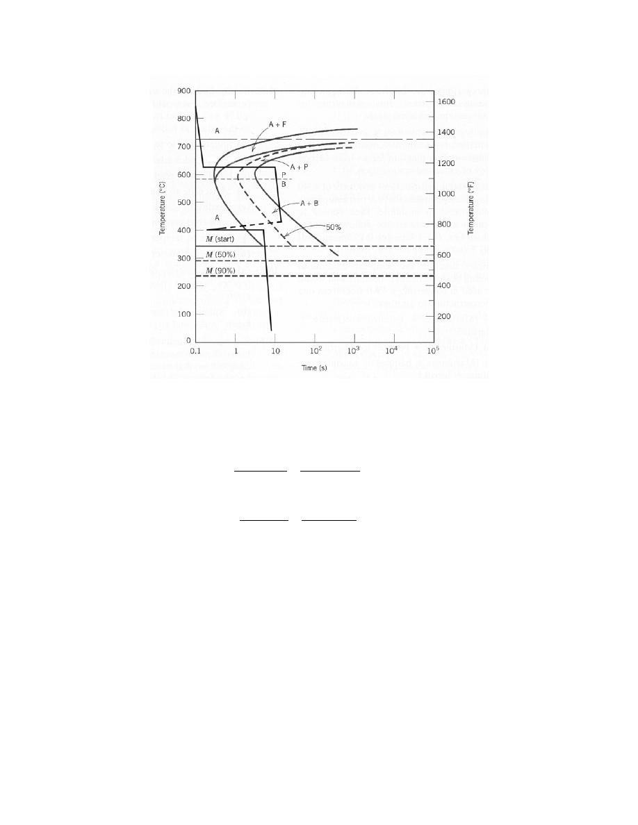
Excerpts from this work may be reproduced by instructors for distribution on a not-for-profit basis for testing or instructional purposes only to
students enrolled in courses for which the textbook has been adopted. Any other reproduction or translation of this work beyond that permitted
by Sections 107 or 108 of the 1976 United States Copyright Act without the permission of the copyright owner is unlawful.
After holding for 10 s at 625
°C, the specimen has completely transformed to proeutectoid ferrite and fine pearlite;
no further reaction will occur at 400
°C. Therefore, we can calculate the mass fractions using the appropriate lever
rule expressions, Equations 9.20 and 9.21, as follows:
W
p
=
C
0
’
− 0.022
0.74
=
0.45
− 0.022
0.74
= 0.58 or 58%
W
α'
=
0.76
− C
0
’
0.74
=
0.76
− 0.45
0.74
= 0.42 or 42%
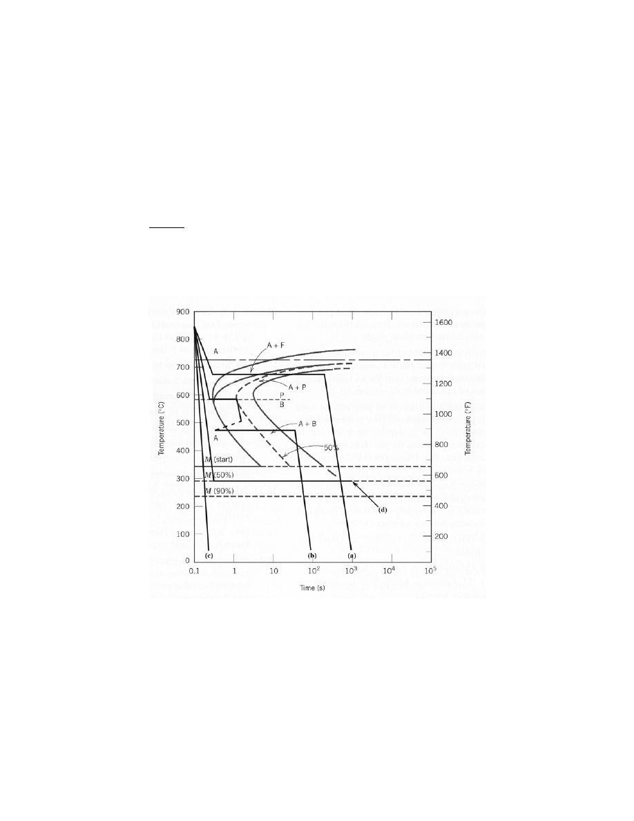
Excerpts from this work may be reproduced by instructors for distribution on a not-for-profit basis for testing or instructional purposes only to
students enrolled in courses for which the textbook has been adopted. Any other reproduction or translation of this work beyond that permitted
by Sections 107 or 108 of the 1976 United States Copyright Act without the permission of the copyright owner is unlawful.
10.22 Make a copy of the isothermal transformation diagram for a 0.45 wt% C iron-carbon alloy (Figure
10.39), and then sketch and label on this diagram the time-temperature paths to produce the following
microstructures:
(a) 42% proeutectoid ferrite and 58% coarse pearlite
(b) 50% fine pearlite and 50% bainite
(c) 100% martensite
(d) 50% martensite and 50% austenite
Solution
Below is shown an isothermal transformation diagram for a 0.45 wt% C iron-carbon alloy, with time-
temperature paths that will produce (a) 42% proeutectoid ferrite and 58% coarse pearlite; (b) 50% fine pearlite and
50% bainite; (c) 100% martensite; and (d) 50% martensite and 50% austenite.

Excerpts from this work may be reproduced by instructors for distribution on a not-for-profit basis for testing or instructional purposes only to
students enrolled in courses for which the textbook has been adopted. Any other reproduction or translation of this work beyond that permitted
by Sections 107 or 108 of the 1976 United States Copyright Act without the permission of the copyright owner is unlawful.
Continuous Cooling Transformation Diagrams
10.23 Name the microstructural products of eutectoid iron–carbon alloy (0.76 wt% C) specimens that are
first completely transformed to austenite, then cooled to room temperature at the following rates:
(a) 200°C/s,
(b) 100°C/s, and
(c) 20°C/s.
Solution
We are called upon to name the microstructural products that form for specimens of an iron-carbon alloy of
eutectoid composition that are continuously cooled to room temperature at a variety of rates. Figure 10.27 is used in
these determinations.
(a) At a rate of 200°C/s, only martensite forms.
(b) At a rate of 100°C/s, both martensite and pearlite form.
(c) At a rate of 20°C/s, only fine pearlite forms.
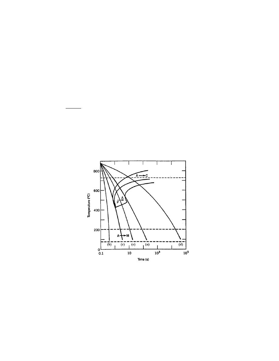
Excerpts from this work may be reproduced by instructors for distribution on a not-for-profit basis for testing or instructional purposes only to
students enrolled in courses for which the textbook has been adopted. Any other reproduction or translation of this work beyond that permitted
by Sections 107 or 108 of the 1976 United States Copyright Act without the permission of the copyright owner is unlawful.
10.24 Figure 10.40 shows the continuous cooling transformation diagram for a 1.13 wt% C iron-carbon
alloy. Make a copy of this figure and then sketch and label continuous cooling curves to yield the following
microstructures:
(a) Fine pearlite and proeutectoid cementite
(b) Martensite
(c) Martensite and proeutectoid cementite
(d) Coarse pearlite and proeutectoid cementite
(e) Martensite, fine pearlite, and proeutectoid cementite
Solution
Below is shown a continuous cooling transformation diagram for a 1.13 wt% C iron-carbon alloy, with
continuous cooling paths that will produce (a) fine pearlite and proeutectoid cementite; (b) martensite; (c)
martensite and proeutectoid cementite; (d) coarse pearlite and proeutectoid cementite; and (e) martensite, fine
pearlite, and proeutectoid cementite.

Excerpts from this work may be reproduced by instructors for distribution on a not-for-profit basis for testing or instructional purposes only to
students enrolled in courses for which the textbook has been adopted. Any other reproduction or translation of this work beyond that permitted
by Sections 107 or 108 of the 1976 United States Copyright Act without the permission of the copyright owner is unlawful.
10.25 Cite two important differences between continuous cooling transformation diagrams for plain
carbon and alloy steels.
Solution
Two important differences between continuous cooling transformation diagrams for plain carbon and alloy
steels are: (1) for an alloy steel, a bainite nose will be present, which nose will be absent for plain carbon alloys;
and (2) the pearlite-proeutectoid noses for plain carbon steel alloys are positioned at shorter times than for the alloy
steels.

Excerpts from this work may be reproduced by instructors for distribution on a not-for-profit basis for testing or instructional purposes only to
students enrolled in courses for which the textbook has been adopted. Any other reproduction or translation of this work beyond that permitted
by Sections 107 or 108 of the 1976 United States Copyright Act without the permission of the copyright owner is unlawful.
10.26 Briefly explain why there is no bainite transformation region on the continuous cooling
transformation diagram for an iron–carbon alloy of eutectoid composition.
Solution
There is no bainite transformation region on the continuous cooling transformation diagram for an iron-
carbon alloy of eutectoid composition (Figure 10.25) because by the time a cooling curve has passed into the bainite
region, the entirety of the alloy specimen will have transformed to pearlite.

Excerpts from this work may be reproduced by instructors for distribution on a not-for-profit basis for testing or instructional purposes only to
students enrolled in courses for which the textbook has been adopted. Any other reproduction or translation of this work beyond that permitted
by Sections 107 or 108 of the 1976 United States Copyright Act without the permission of the copyright owner is unlawful.
10.27 Name the microstructural products of 4340 alloy steel specimens that are first completely
transformed to austenite, then cooled to room temperature at the following rates:
(a) 10°C/s,
(b) 1°C/s,
(c) 0.1°C/s, and
(d) 0.01°C/s.
Solution
This problem asks for the microstructural products that form when specimens of a 4340 steel are
continuously cooled to room temperature at several rates. Figure 10.28 is used for these determinations.
(a) At a cooling rate of 10
°C/s, only martensite forms.
(b) At a cooling rate of 1
°C/s, both martensite and bainite form.
(c) At a cooling rate of 0.1
°C/s, martensite, proeutectoid ferrite, and bainite form.
(d) At a cooling rate of 0.01
°C/s, martensite, proeutectoid ferrite, pearlite, and bainite form.

Excerpts from this work may be reproduced by instructors for distribution on a not-for-profit basis for testing or instructional purposes only to
students enrolled in courses for which the textbook has been adopted. Any other reproduction or translation of this work beyond that permitted
by Sections 107 or 108 of the 1976 United States Copyright Act without the permission of the copyright owner is unlawful.
10.28 Briefly describe the simplest continuous cooling heat treatment procedure that would be used in
converting a 4340 steel from one microstructure to another.
(a) (Martensite + bainite) to (ferrite + pearlite)
(b) (Martensite + bainite) to spheroidite
(c) (Martensite + bainite) to (martensite + bainite + ferrite)
Solution
This problem asks that we briefly describe the simplest continuous cooling heat treatment procedure that
would be used in converting a 4340 steel from one microstructure to another. Solutions to this problem require the
use of Figure 10.28.
(a) In order to convert from (martensite + bainite) to (ferrite + pearlite) it is necessary to heat above about
720
°C, allow complete austenitization, then cool to room temperature at a rate slower than 0.006°C/s.
(b) To convert from (martensite + bainite) to spheroidite the alloy must be heated to about 700
°C for
several hours.
(c) In order to convert from (martensite + bainite) to (martensite + bainite + ferrite) it is necessary to heat
to above about 720
°C, allow complete austenitization, then cool to room temperature at a rate between 0.3°C/s and
0.02
°C/s.

Excerpts from this work may be reproduced by instructors for distribution on a not-for-profit basis for testing or instructional purposes only to
students enrolled in courses for which the textbook has been adopted. Any other reproduction or translation of this work beyond that permitted
by Sections 107 or 108 of the 1976 United States Copyright Act without the permission of the copyright owner is unlawful.
10.29 On the basis of diffusion considerations, explain why fine pearlite forms for the moderate cooling of
austenite through the eutectoid temperature, whereas coarse pearlite is the product for relatively slow cooling
rates.
Solution
For moderately rapid cooling, the time allowed for carbon diffusion is not as great as for slower cooling
rates. Therefore, the diffusion distance is shorter, and thinner layers of ferrite and cementite form (i.e., fine pearlite
forms).

Excerpts from this work may be reproduced by instructors for distribution on a not-for-profit basis for testing or instructional purposes only to
students enrolled in courses for which the textbook has been adopted. Any other reproduction or translation of this work beyond that permitted
by Sections 107 or 108 of the 1976 United States Copyright Act without the permission of the copyright owner is unlawful.
Mechanical Behavior of Iron-Carbon Alloys
Tempered Martensite
10.30 Briefly explain why fine pearlite is harder and stronger than coarse pearlite, which in turn is harder
and stronger than spheroidite.
Solution
The hardness and strength of iron-carbon alloys that have microstructures consisting of
α-ferrite and
cementite phases depend on the boundary area between the two phases. The greater this area, the harder and
stronger the alloy inasmuch as (1) these boundaries impede the motion of dislocations, and (2) the cementite phase
restricts the deformation of the ferrite phase in regions adjacent to the phase boundaries. Fine pearlite is harder and
stronger than coarse pearlite because the alternating ferrite-cementite layers are thinner for fine, and therefore, there
is more phase boundary area. The phase boundary area between the sphere-like cementite particles and the ferrite
matrix is less in spheroidite than for the alternating layered microstructure found in coarse pearlite.

Excerpts from this work may be reproduced by instructors for distribution on a not-for-profit basis for testing or instructional purposes only to
students enrolled in courses for which the textbook has been adopted. Any other reproduction or translation of this work beyond that permitted
by Sections 107 or 108 of the 1976 United States Copyright Act without the permission of the copyright owner is unlawful.
10.31 Cite two reasons why martensite is so hard and brittle.
Solution
Two reasons why martensite is so hard and brittle are: (1) there are relatively few operable slip systems
for the body-centered tetragonal crystal structure, and (2) virtually all of the carbon is in solid solution, which
produces a solid-solution hardening effect.

Excerpts from this work may be reproduced by instructors for distribution on a not-for-profit basis for testing or instructional purposes only to
students enrolled in courses for which the textbook has been adopted. Any other reproduction or translation of this work beyond that permitted
by Sections 107 or 108 of the 1976 United States Copyright Act without the permission of the copyright owner is unlawful.
10.32 Rank the following iron–carbon alloys and associated microstructures from the highest to the
lowest tensile strength:
(a) 0.25 wt%C with spheroidite,
(b) 0.25 wt%C with coarse pearlite,
(c) 0.60 wt%C with fine pearlite, and
(d) 0.60 wt%C with coarse pearlite.
Justify this ranking.
Solution
This problem asks us to rank four iron-carbon alloys of specified composition and microstructure
according to hardness. This ranking is as follows:
0.60 wt% C, fine pearlite
0.60 wt% C, coarse pearlite
0.25 wt% C, coarse pearlite
0.25 wt% C, spheroidite
The 0.25 wt% C, coarse pearlite is stronger than the 0.25 wt% C, spheroidite since coarse pearlite is
stronger than spheroidite; the composition of the alloys is the same. The 0.60 wt% C, coarse pearlite is stronger
than the 0.25 wt% C, coarse pearlite, since increasing the carbon content increases the strength. Finally, the 0.60
wt% C, fine pearlite is stronger than the 0.60 wt% C, coarse pearlite inasmuch as the strength of fine pearlite is
greater than coarse pearlite because of the many more ferrite-cementite phase boundaries in fine pearlite.

Excerpts from this work may be reproduced by instructors for distribution on a not-for-profit basis for testing or instructional purposes only to
students enrolled in courses for which the textbook has been adopted. Any other reproduction or translation of this work beyond that permitted
by Sections 107 or 108 of the 1976 United States Copyright Act without the permission of the copyright owner is unlawful.
10.33 Briefly explain why the hardness of tempered martensite diminishes with tempering time (at
constant temperature) and with increasing temperature (at constant tempering time).
Solution
This question asks for an explanation as to why the hardness of tempered martensite diminishes with
tempering time (at constant temperature) and with increasing temperature (at constant tempering time). The
hardness of tempered martensite depends on the ferrite-cementite phase boundary area; since these phase
boundaries are barriers to dislocation motion, the greater the area the harder the alloy. The microstructure of
tempered martensite consists of small sphere-like particles of cementite embedded within a ferrite matrix. As the
size of the cementite particles increases, the phase boundary area diminishes, and the alloy becomes softer.
Therefore, with increasing tempering time, the cementite particles grow, the phase boundary area decreases, and the
hardness diminishes. As the tempering temperature is increased, the rate of cementite particle growth also
increases, and the alloy softens, again, because of the decrease in phase boundary area.

Excerpts from this work may be reproduced by instructors for distribution on a not-for-profit basis for testing or instructional purposes only to
students enrolled in courses for which the textbook has been adopted. Any other reproduction or translation of this work beyond that permitted
by Sections 107 or 108 of the 1976 United States Copyright Act without the permission of the copyright owner is unlawful.
10.34 Briefly describe the simplest heat treatment procedure that would be used in converting a 0.76 wt%
C steel from one microstructure to the other, as follows:
(a) Spheroidite to tempered martensite
(b) Tempered martensite to pearlite
(c) Bainite to martensite
(d) Martensite to pearlite
(e) Pearlite to tempered martensite
(f) Tempered martensite to pearlite
(g) Bainite to tempered martensite
(h) Tempered martensite to spheroidite
Solution
In this problem we are asked to describe the simplest heat treatment that would be required to convert a
eutectoid steel from one microstructure to another. Figure 10.27 is used to solve the several parts of this problem.
(a) For spheroidite to tempered martensite, austenitize at a temperature of about 760
°C, quench to room
temperature at a rate greater than about 140
°C/s, then isothermally heat at a temperature between 250 and 650°C.
(b) For tempered martensite to pearlite, austenitize at a temperature of about 760
°C, then cool to room
temperature at a rate less than about 35
°C/s.
(c) For bainite to martensite, first austenitize at a temperature of about 760
°C, then quench to room
temperature at a rate greater than about 140
°C/s.
(d) For martensite to pearlite, first austenitize at a temperature of about 760
°C, then cool to room
temperature at a rate less than about 35
°C/s.
(e) For pearlite to tempered martensite, first austenitize at a temperature of about 760
°C, then rapidly
quench to room temperature at a rate greater than about 140
°C/s, then isothermally heat treat (temper) at a
temperature between 250 and 650
°C.
(f) For tempered martensite to pearlite, first austenitize at a temperature of about 760
°C, then cool to room
temperature at a rate less than about 35
°C/s.
(g) For bainite to tempered martensite, first austenitize at a temperature of about 760
°C, then rapidly
quench to room temperature at a rate greater than about 140
°C/s, then isothermally heat treat (temper) at a
temperature between 250 and 650
°C.
(h) For tempered martensite to spheroidite simply heat at about 700
°C for approximately 20 h.

Excerpts from this work may be reproduced by instructors for distribution on a not-for-profit basis for testing or instructional purposes only to
students enrolled in courses for which the textbook has been adopted. Any other reproduction or translation of this work beyond that permitted
by Sections 107 or 108 of the 1976 United States Copyright Act without the permission of the copyright owner is unlawful.
10.35 (a) Briefly describe the microstructural difference between spheroidite and tempered martensite.
(b) Explain why tempered martensite is much harder and stronger.
Solution
(a) Both tempered martensite and spheroidite have sphere-like cementite particles within a ferrite matrix;
however, these particles are much larger for spheroidite.
(b) Tempered martensite is harder and stronger inasmuch as there is much more ferrite-cementite phase
boundary area for the smaller particles; thus, there is greater reinforcement of the ferrite phase, and more phase
boundary barriers to dislocation motion.

Excerpts from this work may be reproduced by instructors for distribution on a not-for-profit basis for testing or instructional purposes only to
students enrolled in courses for which the textbook has been adopted. Any other reproduction or translation of this work beyond that permitted
by Sections 107 or 108 of the 1976 United States Copyright Act without the permission of the copyright owner is unlawful.
10.36 Estimate the Rockwell hardnesses for specimens of an iron–carbon alloy of eutectoid composition
that have been subjected to the heat treatments described in parts (b), (d), (f), (g), and (h) of Problem 10.18.
Solution
This problem asks for estimates of Rockwell hardness values for specimens of an iron-carbon alloy of
eutectoid composition that have been subjected to some of the heat treatments described in Problem 10.18.
(b) The microstructural product of this heat treatment is 100% spheroidite. According to Figure 10.30a,
the hardness of a 0.76 wt% C alloy with spheroidite is about 87 HRB.
(d) The microstructural product of this heat treatment is 100% martensite. According to Figure 10.32, the
hardness of a 0.76 wt% C alloy consisting of martensite is about 64 HRC.
(f) The microstructural product of this heat treatment is 100% bainite. From Figure 10.31, the hardness of
a 0.76 wt% C alloy consisting of bainite is about 385 HB. And, conversion from Brinell to Rockwell hardness
using Figure 6.18 leads to a hardness of 36 HRC.
(g) The microstructural product of this heat treatment is 100% fine pearlite. According to Figure 10.30a,
the hardness of a 0.76 wt% C alloy consisting of fine pearlite is about 27 HRC.
(h) The microstructural product of this heat treatment is 100% tempered martensite. According to Figure
10.35, the hardness of a water-quenched eutectoid alloy that was tempered at 315
°C for one hour is about 57 HRC.

Excerpts from this work may be reproduced by instructors for distribution on a not-for-profit basis for testing or instructional purposes only to
students enrolled in courses for which the textbook has been adopted. Any other reproduction or translation of this work beyond that permitted
by Sections 107 or 108 of the 1976 United States Copyright Act without the permission of the copyright owner is unlawful.
10.37 Estimate the Brinell hardnesses for specimens of a 0.45 wt% C iron-carbon alloy that have been
subjected to the heat treatments described in parts (a), (d), and (h) of Problem 10.20.
Solution
This problem asks for estimates of Brinell hardness values for specimens of an iron-carbon alloy of
composition 0.45 wt% C that have been subjected to some of the heat treatments described in Problem 10.20.
(a) The microstructural product of this heat treatment is 100% martensite. According to Figure 10.32, the
hardness of a 0.45 wt% C alloy consisting of martensite is about 630 HB.
(d) The microstructural product of this heat treatment is 100% spheroidite. According to Figure 10.30a the
hardness of a 0.45 wt% C alloy with spheroidite is about 150 HB.
(h) The microstructural product of this heat treatment is proeutectoid ferrite and fine pearlite. According to
Figure 10.30a, the hardness of a 0.45 wt% C alloy consisting of fine pearlite is about 200 HB.

Excerpts from this work may be reproduced by instructors for distribution on a not-for-profit basis for testing or instructional purposes only to
students enrolled in courses for which the textbook has been adopted. Any other reproduction or translation of this work beyond that permitted
by Sections 107 or 108 of the 1976 United States Copyright Act without the permission of the copyright owner is unlawful.
10.38 Determine the approximate tensile strengths for specimens of a eutectoid iron–carbon alloy that
have experienced the heat treatments described in parts (a) and (c) of Problem 10.23.
Solution
This problem asks for estimates of tensile strength values for specimens of an iron-carbon alloy of
eutectoid composition that have been subjected to some of the heat treatments described in Problem 10.23.
(a) The microstructural product of this heat treatment is 100% martensite. According to Figure 10.32, the
hardness of a 0.76 wt% C alloy is about 690 HB. For steel alloys, hardness and tensile strength are related through
Equation 6.20a, and therefore
TS (MPa) = 3.45
× HB = (3.45)(690 HB) = 2380 MPa (345,000 psi)
(c) The microstructural product of this heat treatment is 100% fine pearlite. According to Figure 10.30a,
the hardness of a 0.76 wt% C alloy consisting of fine pearlite is about 265 HB. Therefore, the tensile strength is
TS (MPa) = 3.45
× HB = (3.45)(265 HB) = 915 MPa (132,500 psi)

Excerpts from this work may be reproduced by instructors for distribution on a not-for-profit basis for testing or instructional purposes only to
students enrolled in courses for which the textbook has been adopted. Any other reproduction or translation of this work beyond that permitted
by Sections 107 or 108 of the 1976 United States Copyright Act without the permission of the copyright owner is unlawful.
10.39 For a eutectoid steel, describe isothermal heat treatments that would be required to yield specimens
having the following Rockwell hardnesses:
(a) 93 HRB,
(b) 40 HRC, and
(c) 27 HRC.
Solution
For this problem we are asked to describe isothermal heat treatments required to yield specimens having
several Brinell hardnesses.
(a) From Figure 10.30a, in order for a 0.76 wt% C alloy to have a Rockwell hardness of 93 HRB, the
microstructure must be coarse pearlite. Thus, utilizing the isothermal transformation diagram for this alloy, Figure
10.22, we must rapidly cool to a temperature at which coarse pearlite forms (i.e., to about 675
°C), allow the
specimen to isothermally and completely transform to coarse pearlite. At this temperature an isothermal heat
treatment for at least 200 s is required.
(b) This portion of the problem asks for a hardness of 40 HRC the microstructure could consist of either (1)
about 75% fine pearlite and 25% martensite (Figure 10.32), or (2) tempered martensite (Figure 10.35).
For case (1), after austenitizing, rapidly cool to about 580
°C (Figure 10.22), hold at this temperature for
about 4 s (to obtain 75% fine pearlite), and then rapidly quench to room temperature.
For case (2), after austenitizing, rapidly cool to room temperature in order to achieve 100% martensite.
Then temper this martensite for about 2000 s at 535
°C (Figure 10.35).
(c) From Figure 10.30a, in order for a 0.76 wt% C alloy to have a Rockwell hardness of 27 HRC, the
microstructure must be fine pearlite. Thus, utilizing the isothermal transformation diagram for this alloy, Figure
10.22, we must rapidly cool to a temperature at which fine pearlite forms (i.e., at about 580
°C), allow the specimen
to isothermally and completely transform to fine pearlite. At this temperature an isothermal heat treatment for at
least 7 s is required.

Excerpts from this work may be reproduced by instructors for distribution on a not-for-profit basis for testing or instructional purposes only to
students enrolled in courses for which the textbook has been adopted. Any other reproduction or translation of this work beyond that permitted
by Sections 107 or 108 of the 1976 United States Copyright Act without the permission of the copyright owner is unlawful.
DESIGN PROBLEMS
Continuous Cooling Transformation Diagrams
Mechanical Behavior of Iron-Carbon Alloys
10.D1 Is it possible to produce an iron-carbon alloy of eutectoid composition that has a minimum
hardness of 90 HRB and a minimum ductility of 35%RA? If so, describe the continuous cooling heat treatment to
which the alloy would be subjected to achieve these properties. If it is not possible, explain why.
Solution
This problem inquires as to the possibility of producing an iron-carbon alloy of eutectoid composition that
has a minimum hardness of 90 HRB and a minimum ductility of 35%RA. If the alloy is possible, then the
continuous cooling heat treatment is to be stipulated.
According to Figures 10.30a and b, the following is a tabulation of Rockwell B hardnesses and percents
area reduction for fine and coarse pearlites and spheroidite for a 0.76 wt% C alloy.
Microstructure
HRB
%RA
Fine pearlite
> 100
20
Coarse pearlite
93
28
Spheroidite
88
67
Therefore, none of the microstructures meets both of these criteria. Both fine and coarse pearlites are hard
enough, but lack the required ductility. Spheroidite is sufficiently ductile, but does not meet the hardness criterion.

Excerpts from this work may be reproduced by instructors for distribution on a not-for-profit basis for testing or instructional purposes only to
students enrolled in courses for which the textbook has been adopted. Any other reproduction or translation of this work beyond that permitted
by Sections 107 or 108 of the 1976 United States Copyright Act without the permission of the copyright owner is unlawful.
10.D2 Is it possible to produce an iron-carbon alloy that has a minimum tensile strength of 690 MPa
(100,000 psi) and a minimum ductility of 40%RA? If so, what will be its composition and microstructure (coarse
and fine pearlites and spheroidite are alternatives)? If this is not possible, explain why.
Solution
This problem asks if it is possible to produce an iron-carbon alloy that has a minimum tensile strength of
690 MPa (100,000 psi) and a minimum ductility of 40%RA. If such an alloy is possible, its composition and
microstructure are to be stipulated.
From Equation 6.20a, this tensile strength corresponds to a Brinell hardness of
HB =
TS (MPa)
3.45
=
690 MPa
3.45
= 200
According to Figures 10.30a and b, the following is a tabulation of the composition ranges for fine and coarse
pearlites and spheroidite that meet the stipulated criteria.
Compositions for
Compositions for
Microstructure
HB
≥ 200
%RA
≥ 40%
Fine pearlite
> 0.45 %C
< 0.47 %C
Coarse pearlite
> 0.7 %C
< 0.54 %C
Spheroidite
not possible
0-1.0 %C
Therefore, only fine pearlite has a composition range overlap for both of the hardness and ductility restrictions; the
fine pearlite would necessarily have to have a carbon content between 0.45 and 0.47 wt% C.

Excerpts from this work may be reproduced by instructors for distribution on a not-for-profit basis for testing or instructional purposes only to
students enrolled in courses for which the textbook has been adopted. Any other reproduction or translation of this work beyond that permitted
by Sections 107 or 108 of the 1976 United States Copyright Act without the permission of the copyright owner is unlawful.
10.D3 It is desired to produce an iron-carbon alloy that has a minimum hardness of 175 HB and a
minimum ductility of 52%RA. Is such an alloy possible? If so, what will be its composition and microstructure
(coarse and fine pearlites and spheroidite are alternatives)? If this is not possible, explain why.
Solution
This problem inquires as to the possibility of producing a iron-carbon alloy having a minimum hardness of
175 HB and a minimum ductility of 52%RA. The composition and microstructure are to be specified; possible
microstructures include fine and coarse pearlites and spheroidite.
To solve this problem, we must consult Figures 10.30a and b. The following is a tabulation of the
composition ranges for fine and coarse pearlites and spheroidite that meet the stipulated criteria.
Compositions for
Compositions for
Microstructure
HB
≥ 175
%RA
≥ 52%
Fine pearlite
> 0.36 %C
< 0.33 %C
Coarse pearlite
> 0.43 %C
< 0.40 %C
Spheroidite
> 0.70
<0-1.0 %C
Thus, only spheroidite has a composition overlap for both of hardness and ductility restrictions; the spheroidite
would necessarily have to have a carbon content greater than 0.70 wt% C.

Excerpts from this work may be reproduced by instructors for distribution on a not-for-profit basis for testing or instructional purposes only to
students enrolled in courses for which the textbook has been adopted. Any other reproduction or translation of this work beyond that permitted
by Sections 107 or 108 of the 1976 United States Copyright Act without the permission of the copyright owner is unlawful.
Tempered Martensite
10.D4 (a) For a 1080 steel that has been water quenched, estimate the tempering time at 425°C (800°F) to
achieve a hardness of 50 HRC.
(b) What will be the tempering time at 315°C (600°F) necessary to attain the same hardness?
Solution
This problem asks us to consider the tempering of a water-quenched 1080 steel to achieve a hardness of 50
HRC. It is necessary to use Figure 10.35.
(a) The time necessary at 425
°C is about 500 s.
(b) At 315
°C, the time required (by extrapolation) is approximately 4 × 10
6
s (about 50 days).

Excerpts from this work may be reproduced by instructors for distribution on a not-for-profit basis for testing or instructional purposes only to
students enrolled in courses for which the textbook has been adopted. Any other reproduction or translation of this work beyond that permitted
by Sections 107 or 108 of the 1976 United States Copyright Act without the permission of the copyright owner is unlawful.
10.D5 An alloy steel (4340) is to be used in an application requiring a minimum tensile strength of 1380
MPa (200,000 psi) and a minimum ductility of 43%RA. Oil quenching followed by tempering is to be used. Briefly
describe the tempering heat treatment.
Solution
We are to consider the tempering of an oil-quenched 4340 steel. From Figure 10.34, for a minimum tensile
strength of 1380 MPa (200,000 psi) a tempering temperature of less than 450
°C (840°F) is required. Also, for a
minimum ductility of 43%RA, tempering must be carried out at a temperature greater than about 400
°C (750°F).
Therefore, tempering must occur at between 400 and 450
°C (750 and 840°F) for 1 h.

Excerpts from this work may be reproduced by instructors for distribution on a not-for-profit basis for testing or instructional purposes only to
students enrolled in courses for which the textbook has been adopted. Any other reproduction or translation of this work beyond that permitted
by Sections 107 or 108 of the 1976 United States Copyright Act without the permission of the copyright owner is unlawful.
10.D6 Is it possible to produce an oil-quenched and tempered 4340 steel that has a minimum yield
strength of 1400 MPa (203,000 psi) and a ductility of at least 42%RA? If this is possible, describe the tempering
heat treatment. If it is not possible, explain why.
Solution
This problem asks if it is possible to produce an oil-quenched and tempered 4340 steel that has a minimum
yield strength of 1400 MPa (203,000 psi) and a minimum ductility of 42%RA, and, if possible, to describe the
tempering heat treatment. In Figure 10.34 is shown the tempering characteristics of this alloy. According to this
figure, in order to achieve a minimum yield strength of 1400 MPa a tempering temperature of less that about 410
°C
is required. On the other hand, tempering must be carried out at greater than about 360
°C for a minimum ductility
of 42%RA. Therefore, an oil-quenched and tempered 4340 alloy possessing these characteristics is possible;
tempering would be carried out at between 360
°C and 410°C for 1 h.

Excerpts from this work may be reproduced by instructors for distribution on a not-for-profit basis for testing or instructional purposes only to
students enrolled in courses for which the textbook has been adopted. Any other reproduction or translation of this work beyond that permitted
by Sections 107 or 108 of the 1976 United States Copyright Act without the permission of the copyright owner is unlawful.
CHAPTER 11
APPLICATIONS AND PROCESSING OF METAL ALLOYS
PROBLEM SOLUTIONS
Ferrous Alloys
11.1 (a) List the four classifications of steels. (b) For each, briefly describe the properties and typical
applications.
Solution
This question asks that we list four classifications of steels, and, for each, to describe properties and cite
typical applications.
Low Carbon Steels
Properties: nonresponsive to heat treatments; relatively soft and weak; machinable and weldable.
Typical applications: automobile bodies, structural shapes, pipelines, buildings, bridges, and tin cans.
Medium Carbon Steels
Properties: heat treatable, relatively large combinations of mechanical characteristics.
Typical applications: railway wheels and tracks, gears, crankshafts, and machine parts.
High Carbon Steels
Properties: hard, strong, and relatively brittle.
Typical applications: chisels, hammers, knives, and hacksaw blades.
High Alloy Steels (Stainless and Tool)
Properties: hard and wear resistant; resistant to corrosion in a large variety of environments.
Typical applications: cutting tools, drills, cutlery, food processing, and surgical tools.

Excerpts from this work may be reproduced by instructors for distribution on a not-for-profit basis for testing or instructional purposes only to
students enrolled in courses for which the textbook has been adopted. Any other reproduction or translation of this work beyond that permitted
by Sections 107 or 108 of the 1976 United States Copyright Act without the permission of the copyright owner is unlawful.
11.2 (a) Cite three reasons why ferrous alloys are used so extensively. (b) Cite three characteristics of
ferrous alloys that limit their utilization.
Solution
(a) Ferrous alloys are used extensively because:
(1) Iron ores exist in abundant quantities.
(2) Economical extraction, refining, and fabrication techniques are available.
(3) The alloys may be tailored to have a wide range of properties.
(b) Disadvantages of ferrous alloys are:
(1) They are susceptible to corrosion.
(2) They have a relatively high density.
(3) They have relatively low electrical conductivities.

Excerpts from this work may be reproduced by instructors for distribution on a not-for-profit basis for testing or instructional purposes only to
students enrolled in courses for which the textbook has been adopted. Any other reproduction or translation of this work beyond that permitted
by Sections 107 or 108 of the 1976 United States Copyright Act without the permission of the copyright owner is unlawful.
11.3 What is the function of alloying elements in tool steels?
Solution
The alloying elements in tool steels (e.g., Cr, V, W, and Mo) combine with the carbon to form very hard
and wear-resistant carbide compounds.

Excerpts from this work may be reproduced by instructors for distribution on a not-for-profit basis for testing or instructional purposes only to
students enrolled in courses for which the textbook has been adopted. Any other reproduction or translation of this work beyond that permitted
by Sections 107 or 108 of the 1976 United States Copyright Act without the permission of the copyright owner is unlawful.
11.4 Compute the volume percent of graphite V
Gr
in a 3.5 wt% C cast iron, assuming that all the carbon
exists as the graphite phase. Assume densities of 7.9 and 2.3 g/cm
3
for ferrite and graphite, respectively.
Solution
We are asked to compute the volume percent graphite in a 3.5 wt% C cast iron. It first becomes necessary
to compute mass fractions using the lever rule. From the iron-carbon phase diagram (Figure 11.2), the tie-line in the
α and graphite phase field extends from essentially 0 wt% C to 100 wt% C. Thus, for a 3.5 wt% C cast iron
W
α
=
C
Gr
− C
0
C
Gr
− C
α
=
100
− 3.5
100
− 0
= 0.965
W
Gr
=
C
0
− C
α
C
Gr
− C
α
=
3.5
− 0
100
− 0
= 0.035
Conversion from weight fraction to volume fraction of graphite is possible using Equation 9.6a as
V
Gr
=
W
Gr
ρ
Gr
W
α
ρ
α
+
W
Gr
ρ
Gr
=
0.035
2.3 g/cm
3
0.965
7.9 g/cm
3
+
0.035
2.3 g/cm
3
= 0.111 or 11.1 vol%

Excerpts from this work may be reproduced by instructors for distribution on a not-for-profit basis for testing or instructional purposes only to
students enrolled in courses for which the textbook has been adopted. Any other reproduction or translation of this work beyond that permitted
by Sections 107 or 108 of the 1976 United States Copyright Act without the permission of the copyright owner is unlawful.
11.5 On the basis of microstructure, briefly explain why gray iron is brittle and weak in tension.
Solution
Gray iron is weak and brittle in tension because the tips of the graphite flakes act as points of stress
concentration.

Excerpts from this work may be reproduced by instructors for distribution on a not-for-profit basis for testing or instructional purposes only to
students enrolled in courses for which the textbook has been adopted. Any other reproduction or translation of this work beyond that permitted
by Sections 107 or 108 of the 1976 United States Copyright Act without the permission of the copyright owner is unlawful.
11.6 Compare gray and malleable cast irons with respect to (a) composition and heat treatment, (b)
microstructure, and (c) mechanical characteristics.
Solution
This question asks us to compare various aspects of gray and malleable cast irons.
(a) With respect to composition and heat treatment:
Gray iron--2.5 to 4.0 wt% C and 1.0 to 3.0 wt% Si. For most gray irons there is no heat treatment
after solidification.
Malleable iron--2.5 to 4.0 wt% C and less than 1.0 wt% Si. White iron is heated in a
nonoxidizing atmosphere and at a temperature between 800 and 900
°C for an extended time period.
(b) With respect to microstructure:
Gray iron--Graphite flakes are embedded in a ferrite or pearlite matrix.
Malleable iron--Graphite clusters are embedded in a ferrite or pearlite matrix.
(c) With respect to mechanical characteristics:
Gray iron--Relatively weak and brittle in tension; good capacity for damping vibrations.
Malleable iron--Moderate strength and ductility.

Excerpts from this work may be reproduced by instructors for distribution on a not-for-profit basis for testing or instructional purposes only to
students enrolled in courses for which the textbook has been adopted. Any other reproduction or translation of this work beyond that permitted
by Sections 107 or 108 of the 1976 United States Copyright Act without the permission of the copyright owner is unlawful.
11.7 Compare white and nodular cast irons with respect to (a) composition and heat treatment, (b)
microstructure, and (c) mechanical characteristics.
Solution
This question asks us to compare white and nodular cast irons.
(a) With regard to composition and heat treatment:
White iron--2.5 to 4.0 wt% C and less than 1.0 wt% Si. No heat treatment; however, cooling is
rapid during solidification.
Nodular cast iron--2.5 to 4.0 wt% C, 1.0 to 3.0 wt% Si, and a small amount of Mg or Ce. A heat
treatment at about 700
°C may be necessary to produce a ferritic matrix.
(b) With regard to microstructure:
White iron--There are regions of cementite interspersed within pearlite.
Nodular cast iron--Nodules of graphite are embedded in a ferrite or pearlite matrix.
(c) With respect to mechanical characteristics:
White iron--Extremely hard and brittle.
Nodular cast iron--Moderate strength and ductility.

Excerpts from this work may be reproduced by instructors for distribution on a not-for-profit basis for testing or instructional purposes only to
students enrolled in courses for which the textbook has been adopted. Any other reproduction or translation of this work beyond that permitted
by Sections 107 or 108 of the 1976 United States Copyright Act without the permission of the copyright owner is unlawful.
11.8 Is it possible to produce malleable cast iron in pieces having large cross-sectional dimensions? Why
or why not?
Solution
It is not possible to produce malleable iron in pieces having large cross-sectional dimensions. White cast
iron is the precursor of malleable iron, and a rapid cooling rate is necessary for the formation of white iron, which
may not be accomplished at interior regions of thick cross-sections.

Excerpts from this work may be reproduced by instructors for distribution on a not-for-profit basis for testing or instructional purposes only to
students enrolled in courses for which the textbook has been adopted. Any other reproduction or translation of this work beyond that permitted
by Sections 107 or 108 of the 1976 United States Copyright Act without the permission of the copyright owner is unlawful.
Nonferrous Alloys
11.9 What is the principal difference between wrought and cast alloys?
Solution
The principal difference between wrought and cast alloys is as follows: wrought alloys are ductile enough
so as to be hot or cold worked during fabrication, whereas cast alloys are brittle to the degree that shaping by
deformation is not possible and they must be fabricated by casting.

Excerpts from this work may be reproduced by instructors for distribution on a not-for-profit basis for testing or instructional purposes only to
students enrolled in courses for which the textbook has been adopted. Any other reproduction or translation of this work beyond that permitted
by Sections 107 or 108 of the 1976 United States Copyright Act without the permission of the copyright owner is unlawful.
11.10 Why must rivets of a 2017 aluminum alloy be refrigerated before they are used?
Solution
Rivets of a 2017 aluminum alloy must be refrigerated before they are used because, after being solution
heat treated, they precipitation harden at room temperature. Once precipitation hardened, they are too strong and
brittle to be driven.

Excerpts from this work may be reproduced by instructors for distribution on a not-for-profit basis for testing or instructional purposes only to
students enrolled in courses for which the textbook has been adopted. Any other reproduction or translation of this work beyond that permitted
by Sections 107 or 108 of the 1976 United States Copyright Act without the permission of the copyright owner is unlawful.
11.11 What is the chief difference between heat-treatable and non-heat-treatable alloys?
Solution
The chief difference between heat-treatable and nonheat-treatable alloys is that heat-treatable alloys may be
strengthened by a heat treatment wherein a precipitate phase is formed (precipitation hardening) or a martensitic
transformation occurs. Nonheat-treatable alloys are not amenable to strengthening by such treatments.

Excerpts from this work may be reproduced by instructors for distribution on a not-for-profit basis for testing or instructional purposes only to
students enrolled in courses for which the textbook has been adopted. Any other reproduction or translation of this work beyond that permitted
by Sections 107 or 108 of the 1976 United States Copyright Act without the permission of the copyright owner is unlawful.
11.12 Give the distinctive features, limitations, and applications of the following alloy groups: titanium
alloys, refractory metals, superalloys, and noble metals.
Solution
Titanium Alloys
Distinctive features: relatively low density, high melting temperatures, and high strengths are possible.
Limitation: because of chemical reactivity with other materials at elevated temperatures, these alloys are
expensive to refine.
Applications: aircraft structures, space vehicles, and in chemical and petroleum industries.
Refractory Metals
Distinctive features: extremely high melting temperatures; large elastic moduli, hardnesses, and strengths.
Limitation: some experience rapid oxidation at elevated temperatures.
Applications: extrusion dies, structural parts in space vehicles, incandescent light filaments, x-ray tubes,
and welding electrodes.
Superalloys
Distinctive features: able to withstand high temperatures and oxidizing atmospheres for long time periods.
Applications: aircraft turbines, nuclear reactors, and petrochemical equipment.
Noble Metals
Distinctive features: highly resistant to oxidation, especially at elevated temperatures; soft and ductile.
Limitation: expensive.
Applications: jewelry, dental restoration materials, coins, catalysts, and thermocouples.

Excerpts from this work may be reproduced by instructors for distribution on a not-for-profit basis for testing or instructional purposes only to
students enrolled in courses for which the textbook has been adopted. Any other reproduction or translation of this work beyond that permitted
by Sections 107 or 108 of the 1976 United States Copyright Act without the permission of the copyright owner is unlawful.
Forming Operations
11.13 Cite advantages and disadvantages of hot working and cold working.
Solution
The advantages of cold working are:
(1) A high quality surface finish.
(2) The mechanical properties may be varied.
(3) Close dimensional tolerances.
The disadvantages of cold working are:
(1) High deformation energy requirements.
(2) Large deformations must be accomplished in steps, which may be expensive.
(3) A loss of ductility.
The advantages of hot working are:
(1) Large deformations are possible, which may be repeated.
(2) Deformation energy requirements are relatively low.
The disadvantages of hot working are:
(1) A poor surface finish.
(2) A variety of mechanical properties is not possible.

Excerpts from this work may be reproduced by instructors for distribution on a not-for-profit basis for testing or instructional purposes only to
students enrolled in courses for which the textbook has been adopted. Any other reproduction or translation of this work beyond that permitted
by Sections 107 or 108 of the 1976 United States Copyright Act without the permission of the copyright owner is unlawful.
11.14 (a) Cite advantages of forming metals by extrusion as opposed to rolling. (b) Cite some
disadvantages.
Solution
(a) The advantages of extrusion as opposed to rolling are as follows:
(1) Pieces having more complicated cross-sectional geometries may be formed.
(2) Seamless tubing may be produced.
(b) The disadvantages of extrusion over rolling are as follows:
(1) Nonuniform deformation over the cross-section.
(2) A variation in properties may result over a cross-section of an extruded piece.

Excerpts from this work may be reproduced by instructors for distribution on a not-for-profit basis for testing or instructional purposes only to
students enrolled in courses for which the textbook has been adopted. Any other reproduction or translation of this work beyond that permitted
by Sections 107 or 108 of the 1976 United States Copyright Act without the permission of the copyright owner is unlawful.
Casting
11.15 List four situations in which casting is the preferred fabrication technique.
Solution
Four situations in which casting is the preferred fabrication technique are:
(1) For large pieces and/or complicated shapes.
(2) When mechanical strength is not an important consideration.
(3) For alloys having low ductilities.
(4) When it is the most economical fabrication technique.

Excerpts from this work may be reproduced by instructors for distribution on a not-for-profit basis for testing or instructional purposes only to
students enrolled in courses for which the textbook has been adopted. Any other reproduction or translation of this work beyond that permitted
by Sections 107 or 108 of the 1976 United States Copyright Act without the permission of the copyright owner is unlawful.
11.16 Compare sand, die, investment, lost foam, and continuous casting techniques.
Solution
For sand casting, sand is the mold material, a two-piece mold is used, ordinarily the surface finish is not an
important consideration, the sand may be reused (but the mold may not), casting rates are low, and large pieces are
usually cast.
For die casting, a permanent mold is used, casting rates are high, the molten metal is forced into the mold
under pressure, a two-piece mold is used, and small pieces are normally cast.
For investment casting, a single-piece mold is used, which is not reusable; it results in high dimensional
accuracy, good reproduction of detail, and a fine surface finish; and casting rates are low.
For lost foam casting, the pattern is polystyrene foam, whereas the mold material is sand. Complex
geometries and tight tolerances are possible. Casting rates are higher than for investment, and there are few
environmental wastes.
For continuous casting, at the conclusion of the extraction process, the molten metal is cast into a
continuous strand having either a rectangular or circular cross-section; these shapes are desirable for subsequent
secondary metal-forming operations. The chemical composition and mechanical properties are relatively uniform
throughout the cross-section.

Excerpts from this work may be reproduced by instructors for distribution on a not-for-profit basis for testing or instructional purposes only to
students enrolled in courses for which the textbook has been adopted. Any other reproduction or translation of this work beyond that permitted
by Sections 107 or 108 of the 1976 United States Copyright Act without the permission of the copyright owner is unlawful.
Miscellaneous Techniques
11.17 If it is assumed that, for steel alloys, the average cooling rate of the heat-affected zone in the vicinity
of a weld is 10°C/s, compare the microstructures and associated properties that will result for 1080 (eutectoid) and
4340 alloys in their HAZs.
Solution
This problem asks that we specify and compare the microstructures and mechanical properties in the heat-
affected weld zones for 1080 and 4340 alloys assuming that the average cooling rate is 10
°C/s. Figure 10.27 shows
the continuous cooling transformation diagram for an iron-carbon alloy of eutectoid composition (1080), and, in
addition, cooling curves that delineate changes in microstructure. For a cooling rate of 10
°C/s (which is less than
35
°C/s) the resulting microstructure will be totally pearlite--probably a reasonably fine pearlite. On the other hand,
in Figure 10.28 is shown the CCT diagram for a 4340 steel. From this diagram it may be noted that a cooling rate of
10
°C/s produces a totally martensitic structure. Pearlite is softer and more ductile than martensite, and, therefore, is
most likely more desirable.

Excerpts from this work may be reproduced by instructors for distribution on a not-for-profit basis for testing or instructional purposes only to
students enrolled in courses for which the textbook has been adopted. Any other reproduction or translation of this work beyond that permitted
by Sections 107 or 108 of the 1976 United States Copyright Act without the permission of the copyright owner is unlawful.
11.18 Describe one problem that might exist with a steel weld that was cooled very rapidly.
Solution
If a steel weld is cooled very rapidly, martensite may form, which is very brittle. In some situations, cracks
may form in the weld region as it cools.

Excerpts from this work may be reproduced by instructors for distribution on a not-for-profit basis for testing or instructional purposes only to
students enrolled in courses for which the textbook has been adopted. Any other reproduction or translation of this work beyond that permitted
by Sections 107 or 108 of the 1976 United States Copyright Act without the permission of the copyright owner is unlawful.
Annealing Processes
11.19 In your own words describe the following heat treatment procedures for steels and, for each, the
intended final microstructure: full annealing, normalizing, quenching, and tempering.
Solution
Full annealing--Heat to about 50
°C above the A
3
line, Figure 11.10 (if the concentration of carbon is less
than the eutectoid) or above the A
1
line (if the concentration of carbon is greater than the eutectoid) until the alloy
comes to equilibrium; then furnace cool to room temperature. The final microstructure is coarse pearlite.
Normalizing--Heat to at least 55
°C above the A
3
line Figure 11.10 (if the concentration of carbon is less
than the eutectoid) or above the A
cm
line (if the concentration of carbon is greater than the eutectoid) until the alloy
completely transforms to austenite, then cool in air. The final microstructure is fine pearlite.
Quenching--Heat to a temperature within the austenite phase region and allow the specimen to fully
austenitize, then quench to room temperature in oil or water. The final microstructure is martensite.
Tempering--Heat a quenched (martensitic) specimen, to a temperature between 450 and 650
°C, for the
time necessary to achieve the desired hardness. The final microstructure is tempered martensite.

Excerpts from this work may be reproduced by instructors for distribution on a not-for-profit basis for testing or instructional purposes only to
students enrolled in courses for which the textbook has been adopted. Any other reproduction or translation of this work beyond that permitted
by Sections 107 or 108 of the 1976 United States Copyright Act without the permission of the copyright owner is unlawful.
11.20 Cite three sources of internal residual stresses in metal components. What are two possible adverse
consequences of these stresses?
Solution
Three sources of residual stresses in metal components are plastic deformation processes, nonuniform
cooling of a piece that was cooled from an elevated temperature, and a phase transformation in which parent and
product phases have different densities.
Two adverse consequences of these stresses are distortion (or warpage) and fracture.

Excerpts from this work may be reproduced by instructors for distribution on a not-for-profit basis for testing or instructional purposes only to
students enrolled in courses for which the textbook has been adopted. Any other reproduction or translation of this work beyond that permitted
by Sections 107 or 108 of the 1976 United States Copyright Act without the permission of the copyright owner is unlawful.
11.21 Give the approximate minimum temperature at which it is possible to austenitize each of the
following iron–carbon alloys during a normalizing heat treatment: (a) 0.20 wt% C, (b) 0.76 wt% C, and (c) 0.95
wt% C.
Solution
(a) For 0.20 wt% C, heat to at least 905
°C (1660°F) since the A
3
temperature is 850
°C (1560°F).
(b) For 0.76 wt% C, heat to at least 782
°C (1440°F) since the A
3
temperature is 727
°C (1340°F).
(c) For 0.95 wt% C, heat to at least 840
°C (1545°F) since the A
cm
temperature is 785
°C (1445°F).

Excerpts from this work may be reproduced by instructors for distribution on a not-for-profit basis for testing or instructional purposes only to
students enrolled in courses for which the textbook has been adopted. Any other reproduction or translation of this work beyond that permitted
by Sections 107 or 108 of the 1976 United States Copyright Act without the permission of the copyright owner is unlawful.
11.22 Give the approximate temperature at which it is desirable to heat each of the following iron–carbon
alloys during a full anneal heat treatment: (a) 0.25 wt% C, (b) 0.45 wt% C, (c) 0.85 wt% C, and (d) 1.10 wt% C.
Solution
(a) For 0.25 wt% C, heat to about 880
°C (1510°F) since the A
3
temperature is 830
°C (1420°F).
(b) For 0.45 wt% C, heat to about 830
°C (1525°F) since the A
3
temperature is 780
°C (1435°F).
(c) For 0.85 wt% C, heat to about 777
°C (1430°F) since the A
1
temperature is 727
°C (1340°F).
(d) For 1.10 wt% C, heat to about 777
°C (1430°F) since the A
1
temperature is 727
°C (1340°F).

Excerpts from this work may be reproduced by instructors for distribution on a not-for-profit basis for testing or instructional purposes only to
students enrolled in courses for which the textbook has been adopted. Any other reproduction or translation of this work beyond that permitted
by Sections 107 or 108 of the 1976 United States Copyright Act without the permission of the copyright owner is unlawful.
11.23 What is the purpose of a spheroidizing heat treatment? On what classes of alloys is it normally
used?
Solution
The purpose of a spheroidizing heat treatment is to produce a very soft and ductile steel alloy having a
spheroiditic microstructure. It is normally used on medium- and high-carbon steels, which, by virtue of carbon
content, are relatively hard and strong.

Excerpts from this work may be reproduced by instructors for distribution on a not-for-profit basis for testing or instructional purposes only to
students enrolled in courses for which the textbook has been adopted. Any other reproduction or translation of this work beyond that permitted
by Sections 107 or 108 of the 1976 United States Copyright Act without the permission of the copyright owner is unlawful.
Heat Treatment of Steels
11.24 Briefly explain the difference between hardness and hardenability.
Solution
Hardness is a measure of a material's resistance to localized surface deformation, whereas hardenability is a
measure of the depth to which a ferrous alloy may be hardened by the formation of martensite. Hardenability is
determined from hardness tests.

Excerpts from this work may be reproduced by instructors for distribution on a not-for-profit basis for testing or instructional purposes only to
students enrolled in courses for which the textbook has been adopted. Any other reproduction or translation of this work beyond that permitted
by Sections 107 or 108 of the 1976 United States Copyright Act without the permission of the copyright owner is unlawful.
11.25 What influence does the presence of alloying elements (other than carbon) have on the shape of a
hardenability curve? Briefly explain this effect.
Solution
The presence of alloying elements (other than carbon) causes a much more gradual decrease in hardness
with position from the quenched end for a hardenability curve. The reason for this effect is that alloying elements
retard the formation of pearlitic and bainitic structures which are not as hard as martensite.

Excerpts from this work may be reproduced by instructors for distribution on a not-for-profit basis for testing or instructional purposes only to
students enrolled in courses for which the textbook has been adopted. Any other reproduction or translation of this work beyond that permitted
by Sections 107 or 108 of the 1976 United States Copyright Act without the permission of the copyright owner is unlawful.
11.26 How would you expect a decrease in the austenite grain size to affect the hardenability of a steel
alloy? Why?
Solution
A decrease of austenite grain size will decrease the hardenability. Pearlite normally nucleates at grain
boundaries, and the smaller the grain size, the greater the grain boundary area, and, consequently, the easier it is for
pearlite to form.

Excerpts from this work may be reproduced by instructors for distribution on a not-for-profit basis for testing or instructional purposes only to
students enrolled in courses for which the textbook has been adopted. Any other reproduction or translation of this work beyond that permitted
by Sections 107 or 108 of the 1976 United States Copyright Act without the permission of the copyright owner is unlawful.
11.27 Name two thermal properties of a liquid medium that will influence its quenching effectiveness.
Solution
The two thermal properties of a liquid medium that influence its quenching effectiveness are thermal
conductivity and heat capacity.
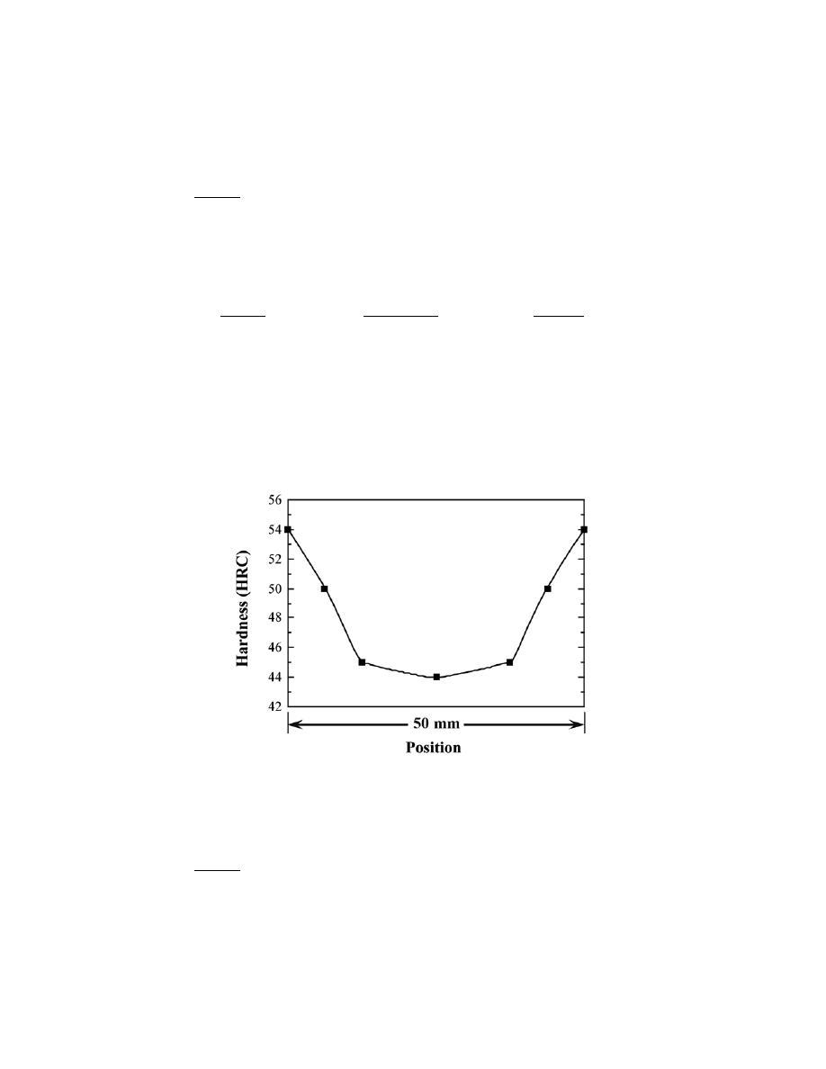
Excerpts from this work may be reproduced by instructors for distribution on a not-for-profit basis for testing or instructional purposes only to
students enrolled in courses for which the textbook has been adopted. Any other reproduction or translation of this work beyond that permitted
by Sections 107 or 108 of the 1976 United States Copyright Act without the permission of the copyright owner is unlawful.
11.28 Construct radial hardness profiles for the following:
(a) A 50-mm (2-in.) diameter cylindrical specimen of an 8640 steel alloy that has been quenched in
moderately agitated oil
Solution
In the manner of Example Problem 11.1, the equivalent distances and hardnesses tabulated below were
determined from Figures 11.14 and 11.17b.
Radial
Equivalent
HRC
Position
Distance, mm
Hardness
Surface
7
54
3/4 R
11
50
Midradius
14
45
Center
16
44
The resulting hardness profile is plotted below.
(b) A 75-mm (3-in.) diameter cylindrical specimen of a 5140 steel alloy that has been quenched in
moderately agitated oil
Solution
In the manner of Example Problem 11.1, the equivalent distances and hardnesses tabulated below were
determined from Figures 11.14 and 11.17b.
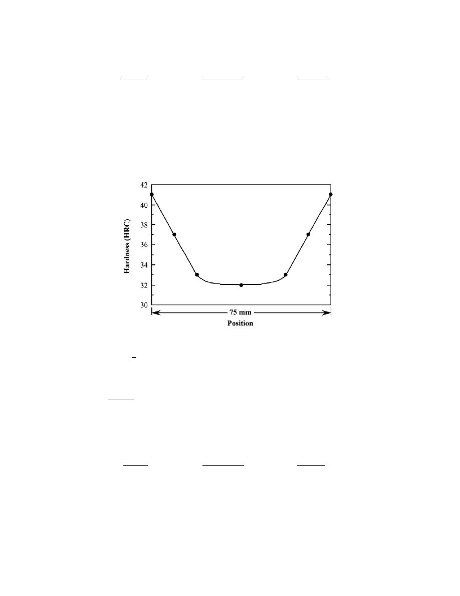
Excerpts from this work may be reproduced by instructors for distribution on a not-for-profit basis for testing or instructional purposes only to
students enrolled in courses for which the textbook has been adopted. Any other reproduction or translation of this work beyond that permitted
by Sections 107 or 108 of the 1976 United States Copyright Act without the permission of the copyright owner is unlawful.
Radial
Equivalent
HRC
Position
Distance, mm
Hardness
Surface
13
41
3/4 R
17.5
37
Midradius
22
33
Center
25
32
The resulting hardness profile is plotted below.
(c) A 65-mm (2
1
2
-in.) diameter cylindrical specimen of an 8620 steel alloy that has been quenched in
moderately agitated water
Solution
In the manner of Example Problem 11.1, the equivalent distances and hardnesses tabulated below were
determined from Figures 11.15 and 11.17a.
Radial
Equivalent
HRC
Position
Distance, mm
Hardness
Surface
2.5
42
3/4 R
7
31
Midradius
11
25
Center
13
24
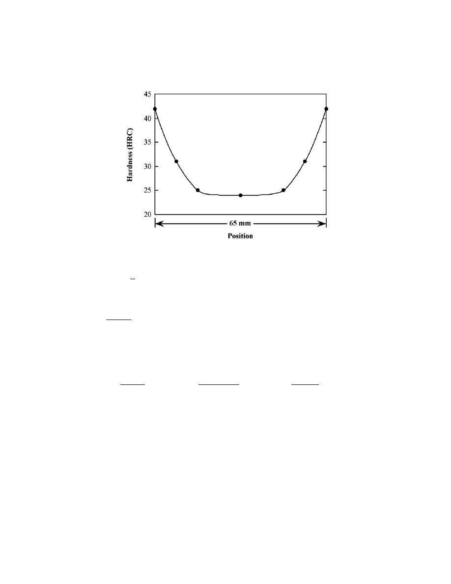
Excerpts from this work may be reproduced by instructors for distribution on a not-for-profit basis for testing or instructional purposes only to
students enrolled in courses for which the textbook has been adopted. Any other reproduction or translation of this work beyond that permitted
by Sections 107 or 108 of the 1976 United States Copyright Act without the permission of the copyright owner is unlawful.
The resulting hardness profile is plotted below.
(d) A 70-mm (2
3
4
-in.) diameter cylindrical specimen of a 1040 steel alloy that has been quenched in
moderately agitated water.
Solution
In the manner of Example Problem 11.1, the equivalent distances and hardnesses tabulated below were
determined from Figures 11.14 and 11.17a.
Radial
Equivalent
HRC
Position
Distance, mm
Hardness
Surface
3
48
3/4 R
8
30
Midradius
13
23
Center
15
22
The resulting hardness profile is plotted below.
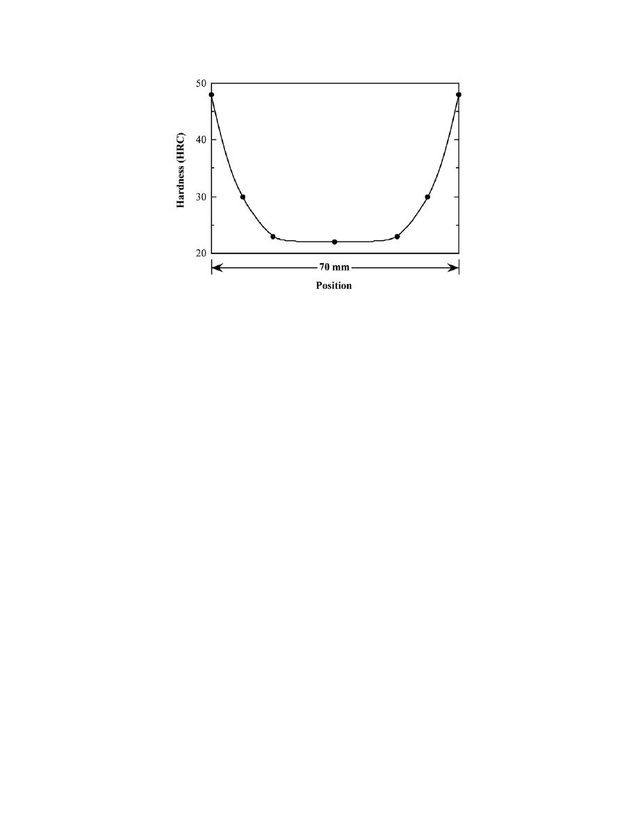
Excerpts from this work may be reproduced by instructors for distribution on a not-for-profit basis for testing or instructional purposes only to
students enrolled in courses for which the textbook has been adopted. Any other reproduction or translation of this work beyond that permitted
by Sections 107 or 108 of the 1976 United States Copyright Act without the permission of the copyright owner is unlawful.
11.29 Compare the effectiveness of quenching in moderately agitated water and oil by graphing, on a
single plot, radial hardness profiles for 65-mm (2
1
2
-in.) diameter cylindrical specimens of an 8630 steel that have
been quenched in both media.
Solution
We are asked to compare the effectiveness of quenching in moderately agitated water and oil by graphing,
on a single plot, hardness profiles for a 65 mm (2-1/2 in.) diameter cylindrical specimen of an 8630 steel that has
been quenched in both media.
For moderately agitated water, the equivalent distances and hardnesses for the several radial positions
[Figures 11.17a and 11.15] are tabulated below.
Radial
Equivalent
HRC
Position
Distance, mm
Hardness
Surface
2.5
52
3/4 R
7
43
Midradius
11
36
Center
13
33
While for moderately agitated oil, the equivalent distances and hardnesses for the several radial positions [Figures
11.17b and 11.15] are tabulated below.
Radial
Equivalent
HRC
Position
Distance, mm
Hardness
Surface
10
37
3/4 R
15
32
Midradius
18
29
Center
20
28
These data are plotted here.
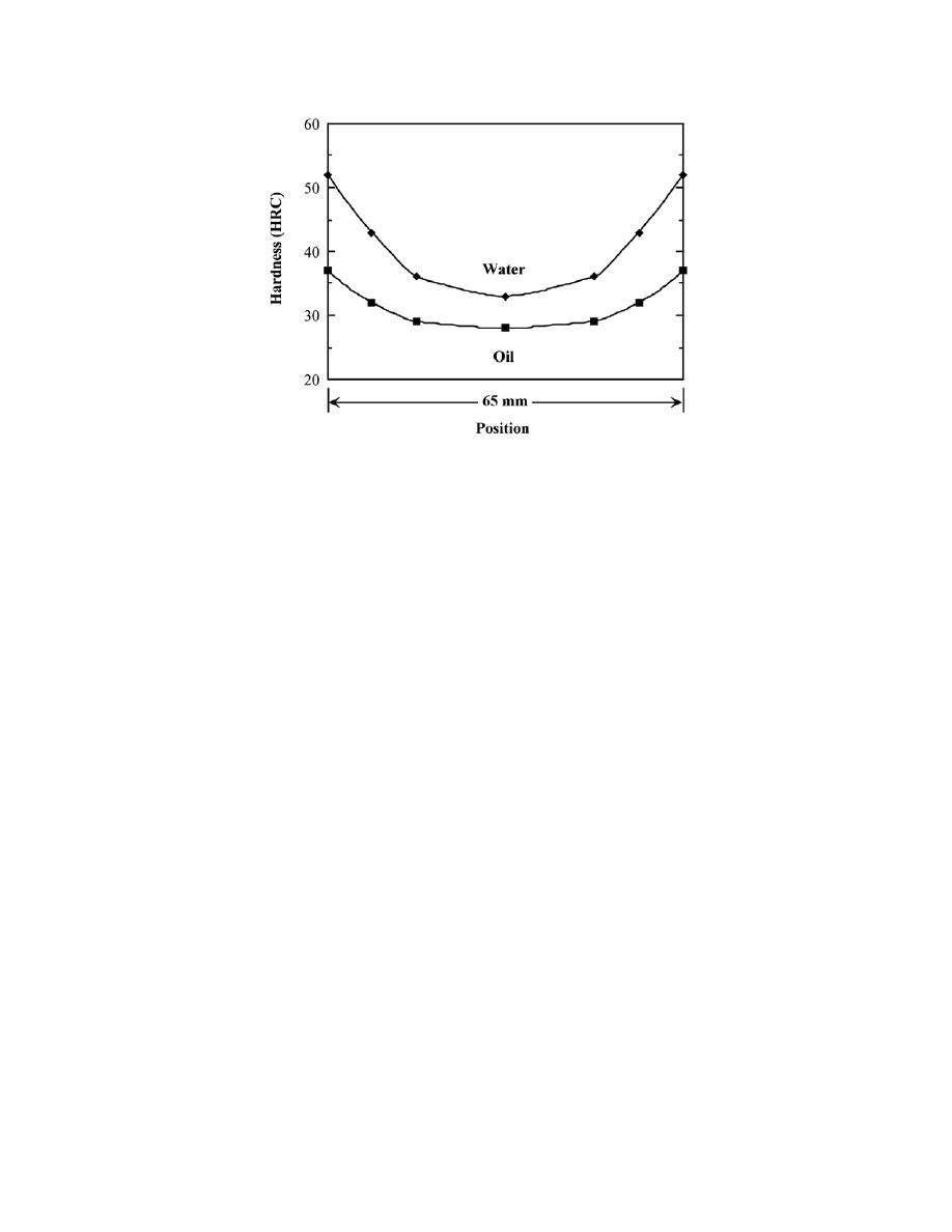
Excerpts from this work may be reproduced by instructors for distribution on a not-for-profit basis for testing or instructional purposes only to
students enrolled in courses for which the textbook has been adopted. Any other reproduction or translation of this work beyond that permitted
by Sections 107 or 108 of the 1976 United States Copyright Act without the permission of the copyright owner is unlawful.
Precipitation Hardening
11.30 Compare precipitation hardening (Section 11.9) and the hardening of steel by quenching and
tempering (Sections 10.5, 10.6, and 10.8) with regard to
(a) The total heat treatment procedure
(b) The microstructures that develop
(c) How the mechanical properties change during the several heat treatment stages
Solution
(a) With regard to the total heat treatment procedure, the steps for the hardening of steel are as follows:
(1) Austenitize above the upper critical temperature.
(2) Quench to a relatively low temperature.
(3) Temper at a temperature below the eutectoid.
(4) Cool to room temperature.
With regard to precipitation hardening, the steps are as follows:
(1) Solution heat treat by heating into the solid solution phase region.
(2) Quench to a relatively low temperature.
(3) Precipitation harden by heating to a temperature that is within the solid two-phase region.
(4) Cool to room temperature.
(b) For the hardening of steel, the microstructures that form at the various heat treating stages in part (a)
are:
(1) Austenite
(2) Martensite
(3) Tempered martensite
(4) Tempered martensite
For precipitation hardening, the microstructures that form at the various heat treating stages in part (a) are:
(1) Single phase
(2) Single phase--supersaturated
(3) Small plate-like particles of a new phase within a matrix of the original phase.
(4) Same as (3)
(c) For the hardening of steel, the mechanical characteristics for the various steps in part (a) are as follows:
(1) Not important
(2) The steel becomes hard and brittle upon quenching.
(3) During tempering, the alloy softens slightly and becomes more ductile.
(4) No significant changes upon cooling to or maintaining at room temperature.

Excerpts from this work may be reproduced by instructors for distribution on a not-for-profit basis for testing or instructional purposes only to
students enrolled in courses for which the textbook has been adopted. Any other reproduction or translation of this work beyond that permitted
by Sections 107 or 108 of the 1976 United States Copyright Act without the permission of the copyright owner is unlawful.
For precipitation hardening, the mechanical characteristics for the various steps in part (a) are as follows:
(1) Not important
(2) The alloy is relatively soft.
(3) The alloy hardens with increasing time (initially), and becomes more brittle; it may soften
with overaging.
(4) The alloy may continue to harden or overage at room temperature.

Excerpts from this work may be reproduced by instructors for distribution on a not-for-profit basis for testing or instructional purposes only to
students enrolled in courses for which the textbook has been adopted. Any other reproduction or translation of this work beyond that permitted
by Sections 107 or 108 of the 1976 United States Copyright Act without the permission of the copyright owner is unlawful.
11.31 What is the principal difference between natural and artificial aging processes?
Solution
For precipitation hardening, natural aging is allowing the precipitation process to occur at the ambient
temperature; artificial aging is carried out at an elevated temperature.

Excerpts from this work may be reproduced by instructors for distribution on a not-for-profit basis for testing or instructional purposes only to
students enrolled in courses for which the textbook has been adopted. Any other reproduction or translation of this work beyond that permitted
by Sections 107 or 108 of the 1976 United States Copyright Act without the permission of the copyright owner is unlawful.
DESIGN PROBLEMS
Ferrous Alloys
Nonferrous Alloys
11.D1 Below is a list of metals and alloys:
Plain carbon steel
Magnesium
Brass
Zinc
Gray cast iron
Tool steel
Platinum
Aluminum
Stainless steel
Tungsten
Titanium alloy
Select from this list the one metal or alloy that is best suited for each of the following applications, and cite at least
one reason for your choice:
(a) The block of an internal combustion engine
(b) Condensing heat exchanger for steam
(c) Jet engine turbofan blades
(d) Drill bit
(e) Cryogenic (i.e., very low temperature) container
(f) As a pyrotechnic (i.e., in flares and fireworks)
(g) High-temperature furnace elements to be used in oxidizing atmospheres
Solution
(a) Gray cast iron would be the best choice for an engine block because it is relatively easy to cast, is wear
resistant, has good vibration damping characteristics, and is relatively inexpensive.
(b) Stainless steel would be the best choice for a heat exchanger to condense steam because it is corrosion
resistant to the steam and condensate.
(c) Titanium alloys are the best choice for high-speed aircraft jet engine turbofan blades because they are
light weight, strong, and easily fabricated very resistant to corrosion. However, one drawback is their cost.
(d) A tool steel would be the best choice for a drill bit because it is very hard retains its hardness at high
temperature and is wear resistant, and, thus, will retain a sharp cutting edge.
(e) For a cryogenic (low-temperature) container, an aluminum alloy would be the best choice; aluminum
alloys have an FCC crystal structure, and therefore, are ductile at very low temperatures.
(f) As a pyrotechnic in flares and fireworks, magnesium is the best choice because it ignites easily and burns

Excerpts from this work may be reproduced by instructors for distribution on a not-for-profit basis for testing or instructional purposes only to
students enrolled in courses for which the textbook has been adopted. Any other reproduction or translation of this work beyond that permitted
by Sections 107 or 108 of the 1976 United States Copyright Act without the permission of the copyright owner is unlawful.
readily in air with a very bright flame.
(g) Platinum is the best choice for high-temperature furnace elements to be used in oxidizing atmospheres
because it is very ductile, has a relatively very high melting temperature, and is highly resistant to oxidation.

Excerpts from this work may be reproduced by instructors for distribution on a not-for-profit basis for testing or instructional purposes only to
students enrolled in courses for which the textbook has been adopted. Any other reproduction or translation of this work beyond that permitted
by Sections 107 or 108 of the 1976 United States Copyright Act without the permission of the copyright owner is unlawful.
11.D2
A group of new materials are the metallic glasses (or amorphous metals). Write an essay about
these materials in which you address the following issues: (1) compositions of some of the common metallic glasses,
(2) characteristics of these materials that make them technologically attractive, (3) characteristics that limit their
utilization, (4) current and potential uses, and (5) at least one technique that is used to produce metallic glasses.
Solution
(a) Compositionally, the metallic glass materials are rather complex; several compositions are as follows:
Fe
80
B
20
, Fe
72
Cr
8
P
13
C
7
, Fe
67
Co
18
B
14
Si, Pd
77.5
Cu
6.0
Si
16.5
, and Fe
40
Ni
38
Mo
4
B
18
.
(b) These materials are exceptionally strong and tough, extremely corrosion resistant, and are easily
magnetized.
(c) Principal drawbacks for these materials are 1) complicated and exotic fabrication techniques are
required; and 2) inasmuch as very rapid cooling rates are required, at least one dimension of the material must be
small--i.e., they are normally produced in ribbon form.
(d) Potential uses include transformer cores, magnetic amplifiers, heads for magnetic tape players,
reinforcements for pressure vessels and tires, shields for electromagnetic interference, security tapes for library
books.
(e) Production techniques include centrifuge melt spinning, planar-flow casting, rapid pressure
application, arc melt spinning.

Excerpts from this work may be reproduced by instructors for distribution on a not-for-profit basis for testing or instructional purposes only to
students enrolled in courses for which the textbook has been adopted. Any other reproduction or translation of this work beyond that permitted
by Sections 107 or 108 of the 1976 United States Copyright Act without the permission of the copyright owner is unlawful.
11.D3 Of the following alloys, pick the one(s) that may be strengthened by heat treatment, cold work, or
both: R50500 titanium, AZ31B magnesium, 6061 aluminum, C51000 phosphor bronze, lead, 6150 steel, 304
stainless steel, and C17200 beryllium copper.
Solution
This question provides us with a list of several metal alloys, and then asks us to pick those that may be
strengthened by heat treatment, by cold work, or both. Those alloys that may be heat treated are either those noted
as "heat treatable" (Tables 11.6 through 11.9), or as martensitic stainless steels (Table 11.4). Alloys that may be
strengthened by cold working must not be exceptionally brittle, and, furthermore, must have recrystallization
temperatures above room temperature (which immediately eliminates lead). The alloys that fall within the three
classifications are as follows:
Heat Treatable
Cold Workable
Both
6150 steel
6150 steel
6150 steel
C17200 Be-Cu
C17200 Be-Cu
C17200 Be-Cu
6061 Al
6061 Al
6061 Al
304 stainless steel
R50500 Ti
C51000 phosphor bronze
AZ31B Mg

Excerpts from this work may be reproduced by instructors for distribution on a not-for-profit basis for testing or instructional purposes only to
students enrolled in courses for which the textbook has been adopted. Any other reproduction or translation of this work beyond that permitted
by Sections 107 or 108 of the 1976 United States Copyright Act without the permission of the copyright owner is unlawful.
11.D4 A structural member 100 mm (4 in.) long must be able to support a load of 50,000 N (11,250 lb
f
)
without experiencing any plastic deformation. Given the following data for brass, steel, aluminum, and titanium,
rank them from least to greatest weight in accordance with these criteria.
Alloy
Yield Strength
[MPa (ksi)]
Density
(g/cm
3
)
Brass
415 (60)
8.5
Steel
860 (125)
7.9
Aluminum
310 (45)
2.7
Titanium
550 (80)
4.5
Solution
This problem asks us to rank four alloys (brass, steel, titanium, and aluminum), from least to greatest
weight for a structural member to support a 50,000 N (11,250 lb
f
) load without experiencing plastic deformation.
From Equation 6.1, the cross-sectional area (A
0
) must necessarily carry the load (F) without exceeding the yield
strength (
σ
y
), as
A
0
=
F
σ
y
Now, given the length l, the volume of material required (V) is just
V = lA
0
=
lF
σ
y
Finally, the mass of the member (m) is
m = V
ρ =
ρ lF
σ
y
Here
ρ is the density. Using the values given for these alloys
m (brass) =
(
8.5 g/cm
3
)
(10 cm)(50, 000 N)
(
415
× 10
6
N / m
2
)
1 m
10
2
cm
2
= 102 g

Excerpts from this work may be reproduced by instructors for distribution on a not-for-profit basis for testing or instructional purposes only to
students enrolled in courses for which the textbook has been adopted. Any other reproduction or translation of this work beyond that permitted
by Sections 107 or 108 of the 1976 United States Copyright Act without the permission of the copyright owner is unlawful.
m (steel) =
(
7.9 g/cm
3
)
(10 cm)(50, 000 N)
(
860
× 10
6
N / m
2
)
1 m
10
2
cm
2
= 46 g
m (aluminum) =
(
2.7 g/cm
3
)
(10 cm)(50, 000 N)
(
310
× 10
6
N / m
2
)
1 m
10
2
cm
2
= 43.5 g
m (titanium) =
(
4.5 g/cm
3
)
(10 cm)(50, 000 N)
(
550
× 10
6
N / m
2
)
1 m
10
2
cm
2
= 40.9 g
Thus, titanium would have the minimum weight (or mass), followed by aluminum, steel, and brass.

Excerpts from this work may be reproduced by instructors for distribution on a not-for-profit basis for testing or instructional purposes only to
students enrolled in courses for which the textbook has been adopted. Any other reproduction or translation of this work beyond that permitted
by Sections 107 or 108 of the 1976 United States Copyright Act without the permission of the copyright owner is unlawful.
11.D5 Discuss whether it would be advisable to hot work or cold work the following metals and alloys on
the basis of melting temperature, oxidation resistance, yield strength, and degree of brittleness: tin, tungsten,
aluminum alloys, magnesium alloys, and a 4140 steel.
Solution
Tin would almost always be hot-worked. Even deformation at room temperature would be considered hot-
working inasmuch as its recrystallization temperature is below room temperature (Table 7.2).
Tungsten is hard and strong at room temperature, has a high recrystallization temperature, and experiences
oxidation at elevated temperatures. Cold-working is difficult because of its strength, and hot-working is not
practical because of oxidation problems. Most tungsten articles are fabricated by powder metallurgy, or by using
cold-working followed by annealing cycles.
Most aluminum alloys may be cold-worked since they are ductile and have relatively low yield strengths.
Magnesium alloys are normally hot-worked inasmuch as they are quite brittle at room temperature. Also,
magnesium alloys have relatively low recrystallization temperatures.
A 4140 steel could be cold-worked in an over-tempered state which leaves it soft and relatively ductile,
after which quenching and tempering heat treatments may be employed to strengthen and harden it. This steel would
probably have a relatively high recrystallization temperature, and hot-working may cause oxidation.

Excerpts from this work may be reproduced by instructors for distribution on a not-for-profit basis for testing or instructional purposes only to
students enrolled in courses for which the textbook has been adopted. Any other reproduction or translation of this work beyond that permitted
by Sections 107 or 108 of the 1976 United States Copyright Act without the permission of the copyright owner is unlawful.
Heat Treatment of Steels
11.D6 A cylindrical piece of steel 25 mm (1.0 in.) in diameter is to be quenched in moderately agitated oil.
Surface and center hardnesses must be at least 55 and 50 HRC, respectively. Which of the following alloys will
satisfy these requirements: 1040, 5140, 4340, 4140, and 8640? Justify your choice(s).
Solution
In moderately agitated oil, the equivalent distances from the quenched end for a one-inch diameter bar for
surface and center positions are 3 mm (1/8 in.) and 8 mm (11/32 in.), respectively [Figure 11.17b]. The hardnesses
at these two positions for the alloys cited (as determined using Figure 11.14) are given below.
Surface
Center
Alloy
Hardness (HRC)
Hardness (HRC)
1040
50
30
5140
56
49
4340
57
57
4140
57
55
8640
57
53
Thus, alloys 4340, 4140, and 8640 will satisfy the criteria for both surface and center hardnesses.

Excerpts from this work may be reproduced by instructors for distribution on a not-for-profit basis for testing or instructional purposes only to
students enrolled in courses for which the textbook has been adopted. Any other reproduction or translation of this work beyond that permitted
by Sections 107 or 108 of the 1976 United States Copyright Act without the permission of the copyright owner is unlawful.
11.D7 A cylindrical piece of steel 75 mm (3 in.) in diameter is to be austenitized and quenched such that a
minimum hardness of 40 HRC is to be produced throughout the entire piece. Of the alloys 8660, 8640, 8630, and
8620, which will qualify if the quenching medium is (a) moderately agitated water, and (b) moderately agitated oil?
Justify your choice(s).
Solution
(a) This problem calls for us to decide which of 8660, 8640, 8630, and 8620 alloys may be fabricated into
a cylindrical piece 75 mm (3 in.) in diameter which, when quenched in mildly agitated water, will produce a
minimum hardness of 40 HRC throughout the entire piece.
The center of the steel cylinder will cool the slowest and therefore will be the softest. In moderately
agitated water the equivalent distance from the quenched end for a 75 mm diameter bar for the center position is
about 17 mm (11/16 in.) [Figure 11.17a]. The hardnesses at this position for the alloys cited (Figure 11.15) are
given below.
Center
Alloy
Hardness (HRC)
8660
58
8640
42
8630
30
8620
22
Therefore, only 8660 and 8640 alloys will have a minimum of 40 HRC at the center, and therefore, throughout the
entire cylinder.
(b) This part of the problem asks us to do the same thing for moderately agitated oil. In moderately
agitated oil the equivalent distance from the quenched end for a 75 mm diameter bar at the center position is about
25.5 mm (1-1/32 in.) [Figure 11.17b]. The hardnesses at this position for the alloys cited (Figure 11.15) are given
below.
Center
Alloy
Hardness (HRC)
8660
53
8640
37
8630
26
8620
< 20

Excerpts from this work may be reproduced by instructors for distribution on a not-for-profit basis for testing or instructional purposes only to
students enrolled in courses for which the textbook has been adopted. Any other reproduction or translation of this work beyond that permitted
by Sections 107 or 108 of the 1976 United States Copyright Act without the permission of the copyright owner is unlawful.
Therefore, only the 8660 alloy will have a minimum of 40 HRC at the center, and therefore, throughout the entire
cylinder.

Excerpts from this work may be reproduced by instructors for distribution on a not-for-profit basis for testing or instructional purposes only to
students enrolled in courses for which the textbook has been adopted. Any other reproduction or translation of this work beyond that permitted
by Sections 107 or 108 of the 1976 United States Copyright Act without the permission of the copyright owner is unlawful.
11.D8 A cylindrical piece of steel 38 mm (1
1
2
in.) in diameter is to be austenitized and quenched such that
a microstructure consisting of at least 80% martensite will be produced throughout the entire piece. Of the alloys
4340, 4140, 8640, 5140, and 1040, which will qualify if the quenching medium is (a) moderately agitated oil and
(b) moderately agitated water? Justify your choice(s).
Solution
(a) Since the cooling rate is lowest at the center, we want a minimum of 80% martensite at the center
position. From Figure 11.17b, the cooling rate is equal to an equivalent distance from the quenched end of 12 mm
(1/2 in.). According to Figure 11.14, the hardness corresponding to 80% martensite for these alloys is 50 HRC.
Thus, all we need do is to determine which of the alloys have a 50 HRC hardness at an equivalent distance from the
quenched end of 12 mm (1/2 in.). At an equivalent distance of 12 mm (1/2 in.), the following hardnesses are
determined from Figure 11.14 for the various alloys.
Alloy
Hardness (HRC)
4340
56
4140
53
8640
49
5140
43
1040
25
Thus, only alloys 4340 and 4140 will qualify.
(b) For moderately agitated water, the cooling rate at the center of a 38 mm diameter specimen is 7 mm
(5/16 in.) equivalent distance from the quenched end [Figure 11.17a]. At this position, the following hardnesses are
determined from Figure 11.14 for the several alloys.
Alloy
Hardness (HRC)
4340
57
4140
55
8640
54
5140
51
1040
33
It is still necessary to have a hardness of 50 HRC or greater at the center; thus, alloys 4340, 4140, 8640, and 5140
qualify.

Excerpts from this work may be reproduced by instructors for distribution on a not-for-profit basis for testing or instructional purposes only to
students enrolled in courses for which the textbook has been adopted. Any other reproduction or translation of this work beyond that permitted
by Sections 107 or 108 of the 1976 United States Copyright Act without the permission of the copyright owner is unlawful.
11.D9 A cylindrical piece of steel 90 mm (3
1
2
in.) in diameter is to be quenched in moderately agitated
water. Surface and center hardnesses must be at least 55 and 40 HRC, respectively. Which of the following alloys
will satisfy these requirements: 1040, 5140, 4340, 4140, 8620, 8630, 8640, and 8660? Justify your choices.
Solution
A ninety-millimeter (three and one-half inch) diameter cylindrical steel specimen is to be quenched in
moderately agitated water. We are to decide which of eight different steels will have surface and center hardnesses
of at least 55 and 40 HRC, respectively.
In moderately agitated water, the equivalent distances from the quenched end for a 90 mm diameter bar for
surface and center positions are 3 mm (1/8 in.) and 22 mm (7/8 in.), respectively [Figure 11.17a]. The hardnesses at
these two positions for the alloys cited are given below. The hardnesses at these two positions for the alloys cited
are given below (as determined from Figures 11.14 and 11.15).
Surface
Center
Alloy
Hardness (HRC)
Hardness (HRC)
1040
50
< 20
5140
56
34
4340
57
53
4140
57
45
8620
42
< 20
8630
51
28
8640
56
38
8660
64
55
Thus, alloys 4340, 4140, and 8660 will satisfy the criteria for both surface hardness (minimum 55 HRC) and center
hardness (minimum 40 HRC).

Excerpts from this work may be reproduced by instructors for distribution on a not-for-profit basis for testing or instructional purposes only to
students enrolled in courses for which the textbook has been adopted. Any other reproduction or translation of this work beyond that permitted
by Sections 107 or 108 of the 1976 United States Copyright Act without the permission of the copyright owner is unlawful.
11.D10 A cylindrical piece of 4140 steel is to be austenitized and quenched in moderately agitated oil. If
the microstructure is to consist of at least 50% martensite throughout the entire piece, what is the maximum
allowable diameter? Justify your answer.
Solution
From Figure 11.14, the equivalent distance from the quenched end of a 4140 steel to give 50% martensite
(or a 42.5 HRC hardness) is 27 mm (1-1/8 in.). Thus, the quenching rate at the center of the specimen should
correspond to this equivalent distance. Using Figure 11.17b, the center specimen curve takes on a value of 27 mm
(1-1/8 in.) equivalent distance at a diameter of about 83 mm (3.3 in.).

Excerpts from this work may be reproduced by instructors for distribution on a not-for-profit basis for testing or instructional purposes only to
students enrolled in courses for which the textbook has been adopted. Any other reproduction or translation of this work beyond that permitted
by Sections 107 or 108 of the 1976 United States Copyright Act without the permission of the copyright owner is unlawful.
11.D11 A cylindrical piece of 8640 steel is to be austenitized and quenched in moderately agitated oil. If
the hardness at the surface of the piece must be at least 49 HRC, what is the maximum allowable diameter? Justify
your answer.
Solution
We are to determine, for a cylindrical piece of 8640 steel, the minimum allowable diameter possible in
order yield a surface hardness of 49 HRC, when the quenching is carried out in moderately agitated oil.
From Figure 11.15, the equivalent distance from the quenched end of an 8640 steel to give a hardness of 49
HRC is about 12 mm (15/32 in.). Thus, the quenching rate at the surface of the specimen should correspond to this
equivalent distance. Using Figure 11.17b, the surface specimen curve takes on a value of 12 mm equivalent
distance at a diameter of about 75 mm (3 in.).

Excerpts from this work may be reproduced by instructors for distribution on a not-for-profit basis for testing or instructional purposes only to
students enrolled in courses for which the textbook has been adopted. Any other reproduction or translation of this work beyond that permitted
by Sections 107 or 108 of the 1976 United States Copyright Act without the permission of the copyright owner is unlawful.
11.D12 Is it possible to temper an oil-quenched 4140 steel cylindrical shaft 100 mm (4 in.) in diameter so
as to give a minimum tensile strength of 850 MPa (125,000 psi) and a minimum ductility of 21%EL? If so, specify a
tempering temperature. If this is not possible, then explain why.
Solution
This problem asks if it is possible to temper an oil-quenched 4140 steel cylindrical shaft 100 mm (4 in.) in
diameter so as to give a minimum tensile strength of 850 MPa (125,000 psi) and a minimum ductility of 21%EL. In
order to solve this problem it is necessary to use Figures 11.20a and 11.20c, which plot, respectively, tensile
strength and ductility versus tempering temperature. For the 100 mm diameter line of Figure 11.20a, tempering
temperatures less than about 560°C are required to give a tensile strength of at least 850 MPa. Furthermore, from
Figure 11.20c, for the 100 mm diameter line, tempering temperatures greater than about 585°C will give ductilities
greater than 21%EL. Hence, it is not possible to temper this alloy to produce the stipulated minimum tensile
strength and ductility. To meet the tensile strength minimum, T(tempering) < 560°C, whereas for ductility
minimum, T(tempering) > 585°C; thus, there is no overlap of these tempering temperature ranges.

Excerpts from this work may be reproduced by instructors for distribution on a not-for-profit basis for testing or instructional purposes only to
students enrolled in courses for which the textbook has been adopted. Any other reproduction or translation of this work beyond that permitted
by Sections 107 or 108 of the 1976 United States Copyright Act without the permission of the copyright owner is unlawful.
11.D13 Is it possible to temper an oil-quenched 4140 steel cylindrical shaft 12.5 mm (0.5 in.) in diameter
so as to give a minimum yield strength of 1000 MPa (145,000 psi) and a minimum ductility of 16%EL? If so,
specify a tempering temperature. If this is not possible, then explain why.
Solution
This problem asks if it is possible to temper an oil-quenched 4140 steel cylindrical shaft 12.5 mm (0.5 in.)
in diameter so as to give a minimum yield strength of 1000 MPa (145,000 psi) and a minimum ductility of 16%EL.
In order to solve this problem it is necessary to use Figures 11.20b and 11.20c, which plot, respectively, yield
strength and ductility versus tempering temperature. For the 12.5 mm diameter line of Figure 11.20b, tempering
temperatures less than about 600°C are required to give a yield strength of at least 1000 MPa. Furthermore, from
Figure 11.20c, for the 12.5 mm diameter line, tempering temperatures greater than about 550°C will give ductilities
greater than 17%EL. Hence, it is possible to temper this alloy to produce the stipulated minimum yield strength and
ductility; the tempering temperature will lie between 550°C and 600°C.
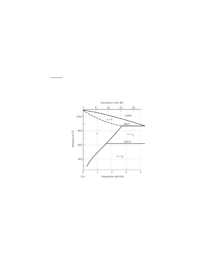
Excerpts from this work may be reproduced by instructors for distribution on a not-for-profit basis for testing or instructional purposes only to
students enrolled in courses for which the textbook has been adopted. Any other reproduction or translation of this work beyond that permitted
by Sections 107 or 108 of the 1976 United States Copyright Act without the permission of the copyright owner is unlawful.
Precipitation Hardening
11.D14 Copper-rich copper–beryllium alloys are precipitation hardenable. After consulting the portion of
the phase diagram (Figure 11.30), do the following:
(a) Specify the range of compositions over which these alloys may be precipitation hardened.
(b) Briefly describe the heat-treatment procedures (in terms of temperatures) that would be used to
precipitation harden an alloy having a composition of your choosing, yet lying within the range given for part (a).
Solution
This problem is concerned with the precipitation-hardening of copper-rich Cu-Be alloys. It is necessary for
us to use the Cu-Be phase diagram (Figure 11.30), which is shown below.
(a) The range of compositions over which these alloys may be precipitation hardened is between
approximately 0.2 wt% Be (the maximum solubility of Be in Cu at about 300
°C) and 2.7 wt% Be (the maximum
solubility of Be in Cu at 866
°C).
(b) The heat treatment procedure, of course, will depend on the composition chosen. First of all, the
solution heat treatment must be carried out at a temperature within the
α phase region, after which, the specimen is
quenched to room temperature. Finally, the precipitation heat treatment is conducted at a temperature within the
α +
γ
2
phase region.
For example, for a 1.5 wt% Be-98.5 wt% Cu alloy, the solution heat treating temperature must be between
about 600
°C (1110°F) and 900°C (1650°F), while the precipitation heat treatment would be below 600°C (1110°F),

Excerpts from this work may be reproduced by instructors for distribution on a not-for-profit basis for testing or instructional purposes only to
students enrolled in courses for which the textbook has been adopted. Any other reproduction or translation of this work beyond that permitted
by Sections 107 or 108 of the 1976 United States Copyright Act without the permission of the copyright owner is unlawful.
and probably above 300
°C (570°F). Below 300°C, diffusion rates are low, and heat treatment times would be
relatively long.

Excerpts from this work may be reproduced by instructors for distribution on a not-for-profit basis for testing or instructional purposes only to
students enrolled in courses for which the textbook has been adopted. Any other reproduction or translation of this work beyond that permitted
by Sections 107 or 108 of the 1976 United States Copyright Act without the permission of the copyright owner is unlawful.
11.D15 A solution heat-treated 2014 aluminum alloy is to be precipitation hardened to have a minimum
tensile strength of 450 MPa (65,250 psi) and a ductility of at least 15%EL. Specify a practical precipitation heat
treatment in terms of temperature and time that would give these mechanical characteristics. Justify your answer.
Solution
We are asked to specify a practical heat treatment for a 2014 aluminum alloy that will produce a minimum
tensile strength of 450 MPa (65,250 psi), and a minimum ductility of 15%EL. From Figure 11.27a, the following
heat treating temperatures and time ranges are possible to the give the required tensile strength.
Temperature (
°C)
Time Range (h)
260
0.02-0.2
204
0.02-10
149
3-600
121
> 35-?
With regard to temperatures and times to give the desired ductility [Figure 11.27b]:
Temperature (
°C)
Time Range (h)
260
< 0.01, > 40
204
< 0.15
149
< 10
121
< 500
From these tabulations, the following may be concluded:
It is not possible to heat treat this alloy at 260
°C so as to produce the desired set of properties— there is no
overlap of the two sets of time ranges.
At 204
°C, the heat treating time would be between 0.02 and 0.15 h; times lying within this range are
impractically short.
At 149
°C, the time would be between 3 and 10 h.
Finally, at 121
°C, the time range is 35 to about 500 h.

Excerpts from this work may be reproduced by instructors for distribution on a not-for-profit basis for testing or instructional purposes only to
students enrolled in courses for which the textbook has been adopted. Any other reproduction or translation of this work beyond that permitted
by Sections 107 or 108 of the 1976 United States Copyright Act without the permission of the copyright owner is unlawful.
11.D16 Is it possible to produce a precipitation-hardened 2014 aluminum alloy having a minimum tensile
strength of 425 MPa (61,625 psi) and a ductility of at least 12%EL? If so, specify the precipitation heat treatment.
If it is not possible, explain why.
Solution
This problem inquires as to the possibility of producing a precipitation-hardened 2014 aluminum alloy
having a minimum tensile strength of 425 MPa (61,625 psi) and a ductility of at least 12%EL. In order to solve this
problem it is necessary to consult Figures 11.27a and 11.27b. Below are tabulated the times required at the various
temperatures to achieve the stipulated tensile strength.
Temperature (
°C)
Time Range (h)
260
< 0.5
204
< 15
149
1-1000
121
> 35-?
With regard to temperatures and times to give the desired ductility:
Temperature (
°C)
Time Range (h)
260
< 0.02, > 10
204
< 0.4, > 350
149
< 20
121
< 1000
From these tabulations, the following may be concluded:
At 260
°C, the heat treating time would need to be less than 0.02 h (1.2 min), which is impractically short.
At 204
°C, the heat treatment would need to be less than 0.4 h (24 min), which is a little on the short side.
At 149
°C, the time range would be between 1 and 20 h.
Finally, at 121
°C, this property combination is possible for virtually all times less than about 1000 h.

Excerpts from this work may be reproduced by instructors for distribution on a not-for-profit basis for testing or instructional purposes only to
students enrolled in courses for which the textbook has been adopted. Any other reproduction or translation of this work beyond that permitted
by Sections 107 or 108 of the 1976 United States Copyright Act without the permission of the copyright owner is unlawful.
CHAPTER 12
STRUCTURES AND PROPERTIES OF CERAMICS
PROBLEM SOLUTIONS
Crystal Structures
12.1 For a ceramic compound, what are the two characteristics of the component ions that determine the
crystal structure?
Solution
The two characteristics of component ions that determine the crystal structure of a ceramic compound are:
1) the magnitude of the electrical charge on each ion, and 2) the relative sizes of the cations and anions.
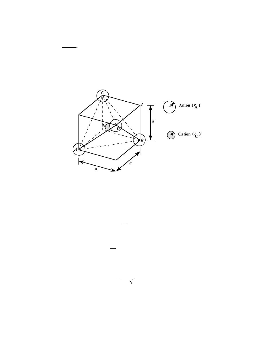
Excerpts from this work may be reproduced by instructors for distribution on a not-for-profit basis for testing or instructional purposes only to
students enrolled in courses for which the textbook has been adopted. Any other reproduction or translation of this work beyond that permitted
by Sections 107 or 108 of the 1976 United States Copyright Act without the permission of the copyright owner is unlawful.
12.2 Show that the minimum cation-to-anion radius ratio for a coordination number of 4 is 0.225.
Solution
In this problem we are asked to show that the minimum cation-to-anion radius ratio for a coordination
number of four is 0.225. If lines are drawn from the centers of the anions, then a tetrahedron is formed. The
tetrahedron may be inscribed within a cube as shown below.
The spheres at the apexes of the tetrahedron are drawn at the corners of the cube, and designated as positions A, B,
C, and D. (These are reduced in size for the sake of clarity.) The cation resides at the center of the cube, which is
designated as point E. Let us now express the cation and anion radii in terms of the cube edge length, designated as
a. The spheres located at positions A and B touch each other along the bottom face diagonal. Thus,
AB = 2 r
A
But
( AB)
2
= a
2
+ a
2
= 2a
2
or
AB = a 2 = 2 r
A
And
Excerpts from this work may be reproduced by instructors for distribution on a not-for-profit basis for testing or instructional purposes only to
students enrolled in courses for which the textbook has been adopted. Any other reproduction or translation of this work beyond that permitted
by Sections 107 or 108 of the 1976 United States Copyright Act without the permission of the copyright owner is unlawful.
a =
2 r
A
2
There will also be an anion located at the corner, point F (not drawn), and the cube diagonal
AEF will be related to
the ionic radii as
AEF = 2
(
r
A
+ r
C
)
(The line AEF has not been drawn to avoid confusion.) From the triangle ABF
( AB)
2
+ (FB)
2
= ( AEF)2
But,
FB = a =
2 r
A
2
and
AB = 2 r
A
from above. Thus,
(
2 r
A
)
2
+
2 r
A
2
2
= 2
(
r
A
+ r
C
)
[
]
2
Solving for the r
C
/r
A
ratio leads to
r
C
r
A
=
6
− 2
2
= 0.225
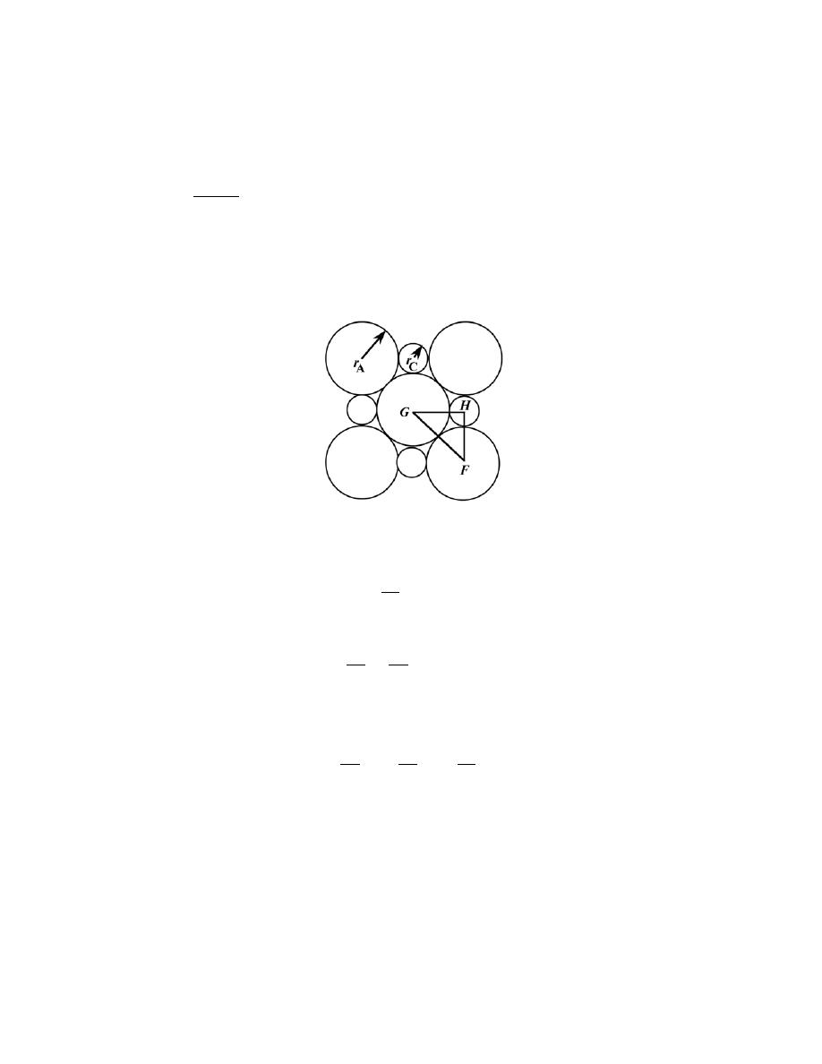
Excerpts from this work may be reproduced by instructors for distribution on a not-for-profit basis for testing or instructional purposes only to
students enrolled in courses for which the textbook has been adopted. Any other reproduction or translation of this work beyond that permitted
by Sections 107 or 108 of the 1976 United States Copyright Act without the permission of the copyright owner is unlawful.
12.3 Show that the minimum cation-to-anion radius ratio for a coordination number of 6 is 0.414. [Hint:
Use the NaCl crystal structure (Figure 12.2), and assume that anions and cations are just touching along cube
edges and across face diagonals.]
Solution
This problem asks us to show that the minimum cation-to-anion radius ratio for a coordination number of 6
is 0.414 (using the rock salt crystal structure). Below is shown one of the faces of the rock salt crystal structure in
which anions and cations just touch along the edges, and also the face diagonals.
From triangle FGH,
GF = 2 r
A
and
FH = GH = r
A
+ r
C
Since FGH is a right triangle
(GH )2 + (FH )2 = (FG)2
or
(
r
A
+ r
C
)
2 +
(
r
A
+ r
C
)
2 =
(
2r
A
)
2
which leads to

Excerpts from this work may be reproduced by instructors for distribution on a not-for-profit basis for testing or instructional purposes only to
students enrolled in courses for which the textbook has been adopted. Any other reproduction or translation of this work beyond that permitted
by Sections 107 or 108 of the 1976 United States Copyright Act without the permission of the copyright owner is unlawful.
r
A
+ r
C
=
2 r
A
2
Or, solving for r
C
/r
A
r
C
r
A
=
2
2
− 1
= 0.414
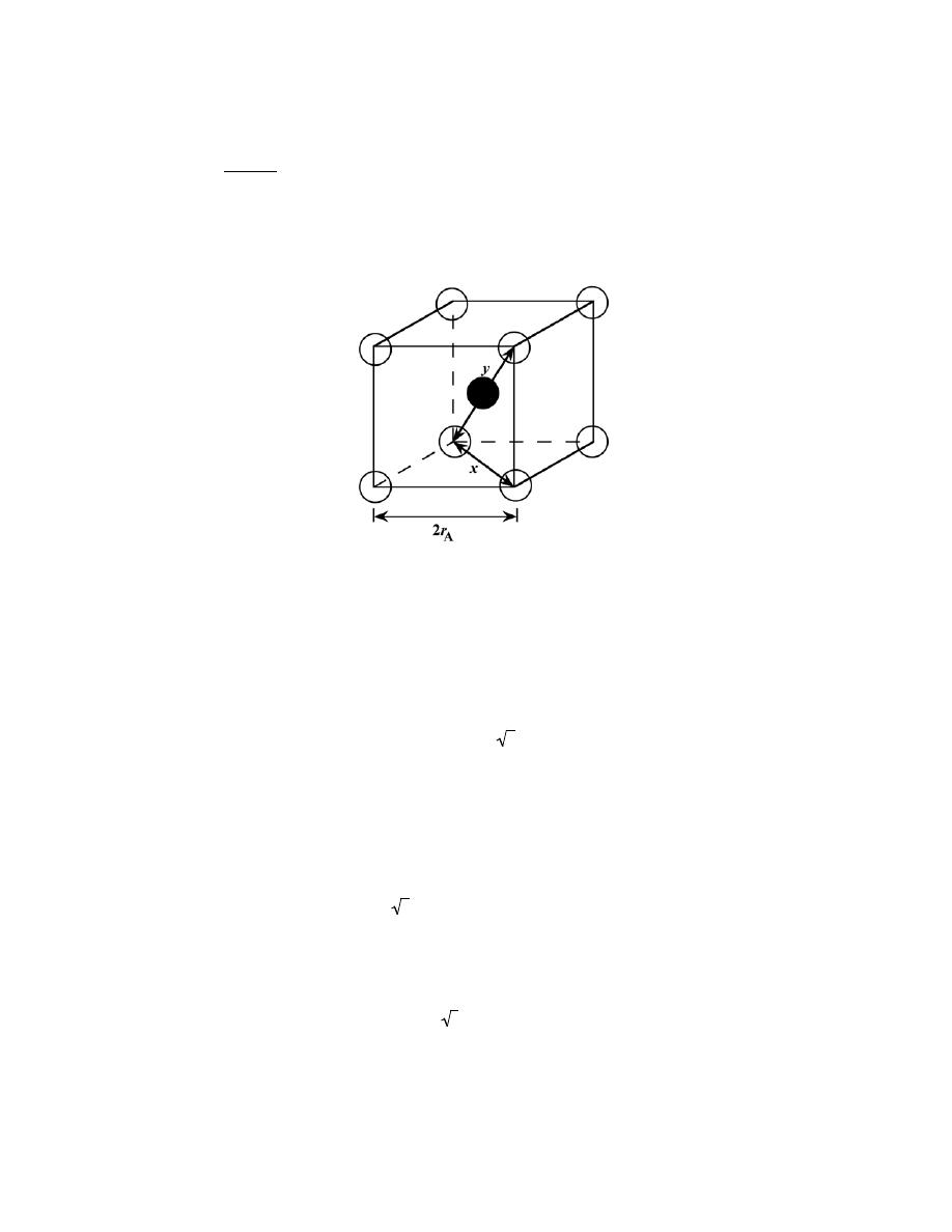
Excerpts from this work may be reproduced by instructors for distribution on a not-for-profit basis for testing or instructional purposes only to
students enrolled in courses for which the textbook has been adopted. Any other reproduction or translation of this work beyond that permitted
by Sections 107 or 108 of the 1976 United States Copyright Act without the permission of the copyright owner is unlawful.
12.4 Demonstrate that the minimum cation-to-anion radius ratio for a coordination number of 8 is 0.732.
Solution
This problem asks us to show that the minimum cation-to-anion radius ratio for a coordination number of 8
is 0.732. From the cubic unit cell shown below
the unit cell edge length is 2r
A
, and from the base of the unit cell
x
2
=
(
2 r
A
)
2
+
(
2 r
A
)
2
= 8 r
A
2
Or
x = 2 r
A
2
Now from the triangle that involves x, y, and the unit cell edge
x
2
+
(
2 r
A
)
2
= y
2
= (2 r
A
+ 2r
C
)
2
(
2 r
A
2
)
2
+ 4 r
A
2
=
(
2 r
A
+ 2 r
C
)
2
Which reduces to
2 r
A
(
3
− 1
)
= 2 r
C
Or

Excerpts from this work may be reproduced by instructors for distribution on a not-for-profit basis for testing or instructional purposes only to
students enrolled in courses for which the textbook has been adopted. Any other reproduction or translation of this work beyond that permitted
by Sections 107 or 108 of the 1976 United States Copyright Act without the permission of the copyright owner is unlawful.
r
C
r
A
= 3
− 1 = 0.732

Excerpts from this work may be reproduced by instructors for distribution on a not-for-profit basis for testing or instructional purposes only to
students enrolled in courses for which the textbook has been adopted. Any other reproduction or translation of this work beyond that permitted
by Sections 107 or 108 of the 1976 United States Copyright Act without the permission of the copyright owner is unlawful.
12.5 On the basis of ionic charge and ionic radii given in Table 12.3, predict crystal structures for the
following materials:
(a) CsI,
(b) NiO,
(c) KI, and
(d) NiS.
Justify your selections.
Solution
This problem calls for us to predict crystal structures for several ceramic materials on the basis of ionic
charge and ionic radii.
(a) For CsI, using data from Table 12.3
r
Cs
+
r
I
−
=
0.170 nm
0.220 nm
= 0.773
Now, from Table 12.2, the coordination number for each cation (Cs
+
) is eight, and, using Table 12.4, the predicted
crystal structure is cesium chloride.
(b) For NiO, using data from Table 12.3
r
Ni
2
+
r
O
2
−
=
0.069 nm
0.140 nm
= 0.493
The coordination number is six (Table 12.2), and the predicted crystal structure is sodium chloride (Table 12.4).
(c) For KI, using data from Table 12.3
r
K
+
r
I
−
=
0.138 nm
0.220 nm
= 0.627
The coordination number is six (Table 12.2), and the predicted crystal structure is sodium chloride (Table 12.4).
(d) For NiS, using data from Table 12.3
r
Ni
2
+
r
S
2
−
=
0.069 nm
0.184 nm
= 0.375
The coordination number is four (Table 12.2), and the predicted crystal structure is zinc blende (Table 12.4).

Excerpts from this work may be reproduced by instructors for distribution on a not-for-profit basis for testing or instructional purposes only to
students enrolled in courses for which the textbook has been adopted. Any other reproduction or translation of this work beyond that permitted
by Sections 107 or 108 of the 1976 United States Copyright Act without the permission of the copyright owner is unlawful.
12.6 Which of the cations in Table 12.3 would you predict to form iodides having the cesium chloride
crystal structure? Justify your choices.
Solution
We are asked to cite the cations in Table 12.3 which would form iodides having the cesium chloride crystal
structure. First of all, the possibilities would include only the monovalent cations Cs
+
, K
+
, and Na
+
. Furthermore,
the coordination number for each cation must be 8, which means that 0.732 < r
C
/r
A
< 1.0 (Table 12.2). From Table
12.3 the r
C
/r
A
ratios for these three cations and the I
-
ion are as follows:
r
Cs
+
r
I
−
=
0.170 nm
0.220 nm
= 0.77
r
K
+
r
I
−
=
0.138 nm
0.220 nm
= 0.63
r
Na
+
r
I
−
=
0.102 nm
0.220 nm
= 0.46
Thus, only cesium will form the CsCl crystal structure with iodine.

Excerpts from this work may be reproduced by instructors for distribution on a not-for-profit basis for testing or instructional purposes only to
students enrolled in courses for which the textbook has been adopted. Any other reproduction or translation of this work beyond that permitted
by Sections 107 or 108 of the 1976 United States Copyright Act without the permission of the copyright owner is unlawful.
12.7 Compute the atomic packing factor for the rock salt crystal structure in which r
C
/r
A
= 0.414.
Solution
This problem asks that we compute the atomic packing factor for the rock salt crystal structure when r
C
/r
A
= 0.414. From Equation 3.2
APF =
V
S
V
C
With regard to the sphere volume, V
S
, there are four cation and four anion spheres per unit cell. Thus,
V
S
= (4)
4
3
π r
A
3
+ (4)
4
3
π r
C
3
But, since r
C
/r
A
= 0.414
V
S
=
16
3
π r
A
3
1
+ (0.414)
3
[
]
= (17.94) r
A
3
Now, for r
C
/r
A
= 0.414 the corner anions in Table 12.2 just touch one another along the cubic unit cell edges such
that
V
C
= a
3
= 2
(
r
A
+ r
C
)
[
]
3
= 2
(
r
A
+ 0.414r
A
)
[
]
3
= (22.62)r
A
3
Thus
APF =
V
S
V
C
=
(17.94) r
A
3
(22.62) r
A
3
= 0.79

Excerpts from this work may be reproduced by instructors for distribution on a not-for-profit basis for testing or instructional purposes only to
students enrolled in courses for which the textbook has been adopted. Any other reproduction or translation of this work beyond that permitted
by Sections 107 or 108 of the 1976 United States Copyright Act without the permission of the copyright owner is unlawful.
12.8 The zinc blende crystal structure is one that may be generated from close-packed planes of anions.
(a) Will the stacking sequence for this structure be FCC or HCP? Why?
(b) Will cations fill tetrahedral or octahedral positions? Why?
(c) What fraction of the positions will be occupied?
Solution
This question is concerned with the zinc blende crystal structure in terms of close-packed planes of anions.
(a) The stacking sequence of close-packed planes of anions for the zinc blende crystal structure will be the
same as FCC (and not HCP) because the anion packing is FCC (Table 12.4).
(b) The cations will fill tetrahedral positions since the coordination number for cations is four (Table
12.4).
(c) Only one-half of the tetrahedral positions will be occupied because there are two tetrahedral sites per
anion, and yet only one cation per anion.
Excerpts from this work may be reproduced by instructors for distribution on a not-for-profit basis for testing or instructional purposes only to
students enrolled in courses for which the textbook has been adopted. Any other reproduction or translation of this work beyond that permitted
by Sections 107 or 108 of the 1976 United States Copyright Act without the permission of the copyright owner is unlawful.
12.9 The corundum crystal structure, found for Al
2
O
3
, consists of an HCP arrangement of O
2-
ions; the
Al
3+
ions occupy octahedral positions.
(a) What fraction of the available octahedral positions are filled with Al
3+
ions?
(b) Sketch two close-packed O
2–
planes stacked in an AB sequence, and note octahedral positions that will
be filled with the Al
3+
ions.
Solution
This question is concerned with the corundum crystal structure in terms of close-packed planes of anions.
(a) For this crystal structure, two-thirds of the octahedral positions will be filled with Al
3+
ions since there
is one octahedral site per O
2-
ion, and the ratio of Al
3+
to O
2-
ions is two-to-three.
(b) Two close-packed O
2-
planes and the octahedral positions between these planes that will be filled with
Al
3+
ions are sketched below.

Excerpts from this work may be reproduced by instructors for distribution on a not-for-profit basis for testing or instructional purposes only to
students enrolled in courses for which the textbook has been adopted. Any other reproduction or translation of this work beyond that permitted
by Sections 107 or 108 of the 1976 United States Copyright Act without the permission of the copyright owner is unlawful.
12.10 Iron sulfide (FeS) may form a crystal structure that consists of an HCP arrangement of S
2-
ions.
(a) Which type of interstitial site will the Fe
2+
ions occupy?
(b) What fraction of these available interstitial sites will be occupied by Fe
2+
ions?
Solution
(a) This portion of the problem asks that we specify which type of interstitial site the Fe
2+
ions will occupy
in FeS if the S
2-
ions form an HCP arrangement. Since, from Table 12.3, r
S
2-
= 0.184 nm and r
Fe
2+
= 0.077 nm,
then
r
Fe
2
+
r
S
2
−
=
0.077 nm
0.184 nm
= 0.418
Inasmuch as rC/rA is between 0.414 and 0.732, the coordination number for Fe
2+
is 6 (Table 12.2); therefore,
tetrahedral octahedral positions are occupied.
(b) We are now asked what fraction of these available interstitial sites are occupied by Fe
2+
ions. Since
there is 1 octahedral site per S
2-
ion, and the ratio of Fe
2+
to S
2-
is 1:1, all of these sites are occupied with Fe
2+
ions.

Excerpts from this work may be reproduced by instructors for distribution on a not-for-profit basis for testing or instructional purposes only to
students enrolled in courses for which the textbook has been adopted. Any other reproduction or translation of this work beyond that permitted
by Sections 107 or 108 of the 1976 United States Copyright Act without the permission of the copyright owner is unlawful.
12.11 Magnesium silicate, Mg
2
SiO
4
, forms in the olivine crystal structure that consists of an HCP
arrangement of O
2-
ions.
(a) Which type of interstitial site will the Mg
2+
ions occupy? Why?
(b) Which type of interstitial site will the Si
4+
ions occupy? Why?
(c) What fraction of the total tetrahedral sites will be occupied?
(d) What fraction of the total octahedral sites will be occupied?
Solution
(a) We are first of all asked to cite, for Mg
2
SiO
4
, which type of interstitial site the Mg
2+
ions will occupy.
From Table 12.3, the cation-anion radius ratio is
r
Mg
2
+
r
O
2
−
=
0.072 nm
0.140 nm
= 0.514
Since this ratio is between 0.414 and 0.732, the Mg
2+
ions will occupy octahedral sites (Table 12.2).
(b) Similarly, for the Si
4+
ions
r
Si
4
+
r
O
2
−
=
0.040 nm
0.140 nm
= 0.286
Since this ratio is between 0.225 and 0.414, the S
i4+
ions will occupy tetrahedral sites.
(c) For each Mg
2
SiO
4
formula unit, there are four O
2-
ions, and, therefore, eight tetrahedral sites;
furthermore, since there is one Si
4+
ion per four O
2-
ions (eight tetrahedral sites), one-eighth of the tetrahedral sites
will be occupied.
(d) Also, inasmuch as the Mg
2+
to O
2-
ratio is 1:2, and there is one octahedral site per O
2-
ion, one-half of
these sites will be filled.
Excerpts from this work may be reproduced by instructors for distribution on a not-for-profit basis for testing or instructional purposes only to
students enrolled in courses for which the textbook has been adopted. Any other reproduction or translation of this work beyond that permitted
by Sections 107 or 108 of the 1976 United States Copyright Act without the permission of the copyright owner is unlawful.
12.12 Using the Molecule Definition Utility found in both “Metallic Crystal Structures and
Crystallography” and “Ceramic Crystal Structures” modules of VMSE, located on the book’s web site
[www.wiley.com/college/callister (Student Companion Site)], generate (and print out) a three-dimensional unit cell
for titanium dioxide, TiO
2
, given the following: (1) The unit cell is tetragonal with a = 0.459 nm and c = 0.296 nm,
(2) oxygen atoms are located at the following point coordinates:
0.356 0.356 0
0.856 0.144
1
2
0.664 0.664 0
0.144 0.856
1
2
and (3) Ti atoms are located at the following point coordinates:
0 0 0
1 0 1
1 0 0
0 1 1
0 1 0
1 1 1
0 0 1
1
2
1
2
1
2
1 1 0
Solution
First of all, open the “Molecular Definition Utility”; it may be found in either of “Metallic Crystal
Structures and Crystallography” or “Ceramic Crystal Structures” modules.
In the “Step 1” window, it is necessary to define the atom types, colors for the spheres (atoms), and specify
atom sizes. Let us enter “O” as the name for the oxygen ions (since “O” the symbol for oxygen), and “Ti” as the
name for the titanium ions. Next it is necessary to choose a color for each atom type from the selections that appear
in the pull-down menu—for example, “Red” for O and “Light Cyan” for Ti. In the “Atom Size” window, it is
necessary to enter an atom/ion size. In the instructions for this step, it is suggested that the atom/ion diameter in
nanometers be used. From the table found inside the front cover of the textbook, the atomic radii for oxygen and
titanium are 0.140 nm and 0.068 nm, respectively, and, therefore, their ionic diameters are twice these values (i.e.,
0.280 nm and 0.136 nm); therefore, we enter the values “0.280” and “0.136” for the two atom types. Now click on
the “Register” button, followed by clicking on the “Go to Step 2” button.
In the “Step 2” window we specify positions for all of the atoms within the unit cell; their point
coordinates are specified in the problem statement. Let’s begin with oxygen. Click on the red sphere that is located
to the right of the “Molecule Definition Utility” box. Some of the point coordinates for the oxygen ions are
fractional ones; in these instances, the unit cell lattice parameters--a or c (i.e., 0.459 or 0.296) are multiplied by the
fraction. For example, one oxygen ion is located at the 0.856 0.144
1
2
coordinate. Therefore, the x, y, and z atoms
positions are (0.856)(0.459) = 0.393, (0.144)(0.459) = 0.066, and
1
2
(0.296) = 0.148, respectively. Thus, we enter
“0.393” in the “x” position box, “0.066” in the “y” position box, and “0.148” in the “z” position box. [Note: the

Excerpts from this work may be reproduced by instructors for distribution on a not-for-profit basis for testing or instructional purposes only to
students enrolled in courses for which the textbook has been adopted. Any other reproduction or translation of this work beyond that permitted
by Sections 107 or 108 of the 1976 United States Copyright Act without the permission of the copyright owner is unlawful.
first two point coordinates relate to the a lattice parameter (0.459 nm), whereas the third applies to the c lattice
parameter (0.296 nm).] Next we click on the “Register Atom Position” button. Now we repeat the procedure for
the remaining oxygen ions
After this step has been completed, it is necessary to specify positions for the titanium ions. To begin, we
click on the light cyan sphere that is located next to the “Molecule Definition Utility” box. One Ti ion will be
positioned at the origin of the coordinate system—i.e., its point coordinates are 0 0 0, and, therefore, we enter a “0”
(zero) in each of the “x”, “y”, and “z” atom position boxes. Next we click on the “Register Atom Position” button.
And the enter the coordinate for all of the other titanium ions
For the oxygen ions, x, y, and z atom position entries for the 4 sets of point coordinates are as follows:
0.163, 0.163, 0
0.305, 0.305, 0
0.393, 0.066, 0.148
0.066, 0.393, 0.148
Now, for the titanium ions, the x, y, and z atom position entries for all 9 sets of point coordinates are as
follows:
0, 0, 0
0.459, 0, 0
0, 0.459, 0
0, 0, 0.296
0.459, 0.459, 0
0.459, 0, 0.296
0, 0.459, 0.296
0.459, 0.459, 0.296
0.230, 0.230, 0.148
In Step 3, we may specify which atoms are to be represented as being bonded to one another, and which
type of bond(s) to use (single solid, single dashed, double, and triple are possibilities), or we may elect to not
represent any bonds at all (in which case we are finished). If it is decided to show bonds, probably the best thing to
do is to represent unit cell edges as bonds. Your resulting image may be rotated by using mouse click-and-drag
Your image should appear as the following screen shot.
Excerpts from this work may be reproduced by instructors for distribution on a not-for-profit basis for testing or instructional purposes only to
students enrolled in courses for which the textbook has been adopted. Any other reproduction or translation of this work beyond that permitted
by Sections 107 or 108 of the 1976 United States Copyright Act without the permission of the copyright owner is unlawful.
Here the darker spheres represent titanium ions, while oxygen ions are depicted by the lighter balls.
[Note: Unfortunately, with this version of the Molecular Definition Utility, it is not possible to save either the data
or the image that you have generated. You may use screen capture (or screen shot) software to record and store
your image.]

Excerpts from this work may be reproduced by instructors for distribution on a not-for-profit basis for testing or instructional purposes only to
students enrolled in courses for which the textbook has been adopted. Any other reproduction or translation of this work beyond that permitted
by Sections 107 or 108 of the 1976 United States Copyright Act without the permission of the copyright owner is unlawful.
12.13 Calculate the density of FeO, given that it has the rock salt crystal structure.
Solution
We are asked to calculate the theoretical density of FeO. This density may be computed using Equation
(12.1) as
ρ =
′
n A
Fe
+ A
O
(
)
V
C
N
A
Since the crystal structure is rock salt, n' = 4 formula units per unit cell. Using the ionic radii for Fe
2+
and O
2-
from
Table 12.3, the unit cell volume is computed as follows:
V
C
= a
3
= 2r
Fe2+
+ 2r
O 2-
(
)
3
= 2 (0.077 nm) + 2 (0.140 nm)
[
]
3
= 0.0817
nm
3
unit cell
= 8.17
× 10
-23
cm
3
unit cell
Thus,
ρ =
(4 formula units/unit cell)(55.85 g/mol + 16.00 g/mol)
8.17
× 10
-23
cm
3
/unit cell
(
)
6.022
× 10
23
formula units/mol
(
)
= 5.84 g/cm
3

Excerpts from this work may be reproduced by instructors for distribution on a not-for-profit basis for testing or instructional purposes only to
students enrolled in courses for which the textbook has been adopted. Any other reproduction or translation of this work beyond that permitted
by Sections 107 or 108 of the 1976 United States Copyright Act without the permission of the copyright owner is unlawful.
12.14 Magnesium oxide has the rock salt crystal structure and a density of 3.58 g/cm
3
.
(a) Determine the unit cell edge length.
(b) How does this result compare with the edge length as determined from the radii in Table 12.3,
assuming that the Mg
2+
and O
2-
ions just touch each other along the edges?
Solution
(a) This part of the problem calls for us to determine the unit cell edge length for MgO. The density of
MgO is 3.58 g/cm
3
and the crystal structure is rock salt. From Equation 12.1
ρ =
′
n
(
A
Mg
+ A
O
)
V
C
N
A
=
′
n
(
A
Mg
+ A
O
)
a
3
N
A
Or, solving for a
a
=
′
n
(
A
Mg
+ A
O
)
ρ N
A
1/ 3
Inasmuch as there are 4 formula units per unit cell for the rock salt crystal structure, and the atomic weights of
magnesium and oxygen are 24.31 and 16.00 g/mol, respectively, when we solve for a from the above equation
a
=
(4 formula units/unit cell)(24.31 g/mol + 16.00 g/mol)
(
3.58 g/cm
3
)(
6.022
× 10
23
formula units/mol
)
1/ 3
= 4.21
× 10
-8
cm = 0.421 nm
(b) The edge length is determined from the Mg
2+
and O
2-
radii for this portion of the problem. Now for
the rock salt crystal structure
a = 2 r
Mg
2+
+ 2 r
O
2-
From Table 12.3
a = 2(0.072 nm) + 2(0.140 nm) = 0.424 nm
Excerpts from this work may be reproduced by instructors for distribution on a not-for-profit basis for testing or instructional purposes only to
students enrolled in courses for which the textbook has been adopted. Any other reproduction or translation of this work beyond that permitted
by Sections 107 or 108 of the 1976 United States Copyright Act without the permission of the copyright owner is unlawful.
12.15 Compute the theoretical density of diamond given that the C—C distance and bond angle are 0.154
nm and 109.5°, respectively. How does this value compare with the measured density?
Solution
This problem asks that we compute the theoretical density of diamond given that the C—C distance and
bond angle are 0.154 nm and 109.5
°, respectively. The first thing we need do is to determine the unit cell edge
length from the given C—C distance. The drawing below shows the cubic unit cell with those carbon atoms that
bond to one another in one-quarter of the unit cell.
From this figure,
φ is one-half of the bond angle or φ = 109.5°/2 = 54.75°, which means that
θ = 90° − 54.75° = 35.25°
since the triangle shown is a right triangle. Also, y = 0.154 nm, the carbon-carbon bond distance.
Furthermore, x = a/4, and therefore,
x =
a
4
= y sin
θ
Or
a = 4 y sin
θ = (4)(0.154 nm)(sin 35.25°) = 0.356 nm
= 3.56
× 10
-8
cm
The unit cell volume, V
C
is just a
3
, that is
V
C
= a
3
=
(
3.56
× 10
-8
cm
)
3
= 4.51 × 10
−23
cm
3

Excerpts from this work may be reproduced by instructors for distribution on a not-for-profit basis for testing or instructional purposes only to
students enrolled in courses for which the textbook has been adopted. Any other reproduction or translation of this work beyond that permitted
by Sections 107 or 108 of the 1976 United States Copyright Act without the permission of the copyright owner is unlawful.
We must now utilize a modified Equation 12.1 since there is only one atom type. There are 8 equivalent atoms per
unit cell, and therefore
ρ =
nÕA
C
V
C
N
A
=
(8 atoms/unit cell)(12.01 g/g - atom)
(
4.51
× 10
-23
cm
3
/unit cell
)(
6.022
× 10
23
atoms/g - atom
)
= 3.54 g/cm
3
The measured density is 3.51 g/cm
3
.

Excerpts from this work may be reproduced by instructors for distribution on a not-for-profit basis for testing or instructional purposes only to
students enrolled in courses for which the textbook has been adopted. Any other reproduction or translation of this work beyond that permitted
by Sections 107 or 108 of the 1976 United States Copyright Act without the permission of the copyright owner is unlawful.
12.16 Compute the theoretical density of ZnS given that the Zn—S distance and bond angle are 0.234 nm
and 109.5°, respectively. How does this value compare with the measured density?
Solution
This problem asks that we compute the theoretical density of ZnS given that the Zn—S distance and bond
angle are 0.234 nm and 109.5
°, respectively. The first thing we need do is to determine the unit cell volume from
the given Zn—S distance. From the previous problem, the unit cell volume V
C
is just a
3
, a being the unit cell edge
length, and
V
C
=
(
4 y sin
θ
)
3 = (4)(0.234 nm)(sin 35.25°)
[
]
3
= 0.1576 nm
3
= 1.576
× 10
-22
cm
3
Now we must utilize Equation 12.1 with n' = 4 formula units, and A
Zn
and A
S
being 65.41 and 32.06 g/mol,
respectively. Thus
ρ =
n'Ê
(
A
Zn
+ A
S
)
V
C
N
A
=
(4 formula units/unit cell)(65.41 g/mol + 32.06 g/mol)
(
1.576
× 10
-22
cm
3
/unit cell
)(
6.022
× 10
23
formula units/mol
)
= 4.11 g/cm
3
The measured value of the density is 4.10 g/cm
3
.

Excerpts from this work may be reproduced by instructors for distribution on a not-for-profit basis for testing or instructional purposes only to
students enrolled in courses for which the textbook has been adopted. Any other reproduction or translation of this work beyond that permitted
by Sections 107 or 108 of the 1976 United States Copyright Act without the permission of the copyright owner is unlawful.
12.17 Cadmium sulfide (CdS) has a cubic unit cell, and from x-ray diffraction data it is known that the cell
edge length is 0.582 nm. If the measured density is 4.82 g/cm
3
, how many Cd
2+
and S
2-
ions are there per unit cell?
Solution
We are asked to determine the number of Cd
2+
and S
2-
ions per unit cell for cadmium sulfide (CdS). For
CdS, a = 0.582 nm and
ρ = 4.82 g/cm
3
. Solving for
n' from Equation 12.1, we get
′
n =
ρV
C
N
A
A
Cd
+ A
S
=
ρa
3
N
A
A
Cd
+ A
S
=
(4.82 g/cm
3
)(5.82
× 10
−8
cm)
3
(6.022
× 10
23
formula units / mol)
(112.41 g/mol
+ 32.06 g/mol)
= 3.96 or almost 4
Therefore, there are four Cd
2+
and four S
2-
per unit cell.
Excerpts from this work may be reproduced by instructors for distribution on a not-for-profit basis for testing or instructional purposes only to
students enrolled in courses for which the textbook has been adopted. Any other reproduction or translation of this work beyond that permitted
by Sections 107 or 108 of the 1976 United States Copyright Act without the permission of the copyright owner is unlawful.
12.18 (a) Using the ionic radii in Table 12.3, compute the theoretical density of CsCl. (Hint: Use a
modification of the result of Problem 3.3.)
(b) The measured density is 3.99 g/cm
3
. How do you explain the slight discrepancy between your
calculated value and the measured one?
Solution
(a) We are asked to compute the density of CsCl. Modifying the result of Problem 3.3, we get
a =
2 r
Cs
+
+ 2r
Cl
−
3
=
2 (0.170 nm)
+ 2 (0.181 nm)
3
= 0.405 nm = 4.05
× 10
-8
cm
From Equation 12.1
ρ = ′
n
(
A
Cs
+ A
Cl
)
VC N
A
=
′
n
(
A
Cs
+ A
Cl
)
a
3
N
A
For the CsCl crystal structure, n' = 1 formula unit/unit cell, and thus
ρ =
(1 formula unit/unit cell)(132.91 g/mol + 35.45 g/mol)
(
4.05
× 10
-8
cm
)
3
/unit cell
(
6.022
× 10
23
formula units/mol
)
= 4.21 g/cm
3
(b) This value of the density is greater than the measured density (3.99 g/cm
3
). The reason for this
discrepancy is that the ionic radii in Table 12.3, used for this computation, were for a coordination number of six,
when, in fact, the coordination number of both Cs
+
and Cl-
is eight. The ionic radii should be slightly greater,
leading
to a larger V
C
value, and a lower density.
Excerpts from this work may be reproduced by instructors for distribution on a not-for-profit basis for testing or instructional purposes only to
students enrolled in courses for which the textbook has been adopted. Any other reproduction or translation of this work beyond that permitted
by Sections 107 or 108 of the 1976 United States Copyright Act without the permission of the copyright owner is unlawful.
12.19 From the data in Table 12.3, compute the theoretical density of CaF
2
, which has the fluorite
structure.
Solution
A unit cell of the fluorite structure is shown in Figure 12.5. It may be seen that there are four CaF
2
units
per unit cell (i.e., n' = 4 formula units/unit cell). Assume that for each of the eight small cubes in the unit cell
a =
2 r
Ca
2
+
+ 2r
F
−
3
and, from Table 12.3
a =
2 (0.100 nm)
+ 2 (0.133 nm)
3
= 0.269 nm = 2.69
× 10
-8
cm
The volume of the unit cell is just
V
C
= (2a)
3
= (2)
(
2.69
× 10
-8
cm
)
[
]
3
= 1.56 × 10
−22
cm
3
Thus, from Equation 12.1
ρ =
n'Ê
(
A
Ca
+ 2 A
F
)
V
C
N
A
=
(4 formula units/unit cell) 40.08 g/mol + (2)(19.00 g/mol)
[
]
(
1.56
× 10
-22
cm
3
/unit cell
)(
6.022
× 10
23
formula units/mol
)
= 3.33 g/cm
3
The measured density is 3.18 g/cm
3
.

Excerpts from this work may be reproduced by instructors for distribution on a not-for-profit basis for testing or instructional purposes only to
students enrolled in courses for which the textbook has been adopted. Any other reproduction or translation of this work beyond that permitted
by Sections 107 or 108 of the 1976 United States Copyright Act without the permission of the copyright owner is unlawful.
12.20 A hypothetical AX type of ceramic material is known to have a density of 2.65 g/cm
3
and a unit cell
of cubic symmetry with a cell edge length of 0.43 nm. The atomic weights of the A and X elements are 86.6 and
40.3 g/mol, respectively. On the basis of this information, which of the following crystal structures is (are) possible
for this material: rock salt, cesium chloride, or zinc blende? Justify your choice(s).
Solution
We are asked to specify possible crystal structures for an AX type of ceramic material given its density
(2.65 g/cm
3
), that the unit cell has cubic symmetry with edge length of 0.43 nm (4.3
× 10
-8
cm), and the atomic
weights of the A and X elements (86.6 and 40.3 g/mol, respectively). Using Equation 12.1 and solving for n' yields
n'
=
ρV
C
N
A
A
C
+
A
A
∑
∑
=
(
2.65 g/cm
3
)
(
4.30
× 10
-8
cm
)
3
/unit cell
[
]
(
6.022
× 10
23
formula units/mol
)
(86.6 + 40.3) g/mol
= 1.00 formula units/unit cell
Of the three possible crystal structures, only cesium chloride has one formula unit per unit cell, and therefore, is the
only possibility.

Excerpts from this work may be reproduced by instructors for distribution on a not-for-profit basis for testing or instructional purposes only to
students enrolled in courses for which the textbook has been adopted. Any other reproduction or translation of this work beyond that permitted
by Sections 107 or 108 of the 1976 United States Copyright Act without the permission of the copyright owner is unlawful.
12.21 The unit cell for MgFe
2
O
4
(MgO-Fe
2
O
3
) has cubic symmetry with a unit cell edge length of 0.836
nm. If the density of this material is 4.52 g/cm
3
, compute its atomic packing factor. For this computation, you will
need to use ionic radii listed in Table 12.3.
Solution
This problem asks us to compute the atomic packing factor for MgFe
2
O
4
given its density and unit cell
edge length. It is first necessary to determine the number of formula units in the unit cell in order to calculate the
sphere volume. Solving for n' from Equation 12.1 leads to
n'
=
ρV
C
N
A
A
C
+
A
A
∑
∑
=
(
4.52 g/cm
3
)
(
8.36
× 10
-8
cm
)
3
/unit cell
[
]
(
6.022
× 10
23
formula units/mol
)
(1)(24.31 g/mol) + (2)(55.85 g/mol) + (4)(16.00 g/mol)
= 8.0 formula units/unit cell
Thus, in each unit cell there are 8 Mg
2+
, 16 Fe
3+
, and 32 O
2-
ions. From Table 12.3, r
Mg
2+
= 0.072 nm, r
Fe
3+
=
0.069 nm, and r
O
2-
= 0.140 nm. Thus, the total sphere volume in Equation 3.2 (which we denote as V
S
), is just
V
S
= (8)
4
3
π
(
7.2
× 10
−9
cm
)
3
+ (16)
4
3
π
(
6.9
× 10
−9
cm
)
3
+ (32)
4
3
π
(
1.40
× 10
−8
cm
)
3
= 4.02
× 10
-22
cm
3
Now, the unit cell volume (V
C
) is just
V
C
= a
3
=
(
8.36
× 10
-8
cm
)
3
= 5.84 × 10
−22
cm
3
Finally, the atomic packing factor (APF) from Equation 3.2 is just
APF
=
V
S
V
C
=
4.02
× 10
-22
cm
3
5.84
× 10
-22
cm
3
= 0.688
Excerpts from this work may be reproduced by instructors for distribution on a not-for-profit basis for testing or instructional purposes only to
students enrolled in courses for which the textbook has been adopted. Any other reproduction or translation of this work beyond that permitted
by Sections 107 or 108 of the 1976 United States Copyright Act without the permission of the copyright owner is unlawful.
12.22 The unit cell for Cr
2
O
3
has hexagonal symmetry with lattice parameters a = 0.4961 nm and c =
1.360 nm. If the density of this material is 5.22 g/cm
3
, calculate its atomic packing factor. For this computation
assume ionic radii of 0.062 nm and 0.140 nm, respectively for Cr
3+
and O
2-
.
Solution
This problem asks for us to calculate the atomic packing factor for chromium oxide given values for the a
and c lattice parameters, and the density. It first becomes necessary to determine the value of n' in Equation 12.1.
This necessitates that we calculate the value of V
C
, the unit cell volume. In Problem 3.6 it was shown that the area
of the hexagonal base (AREA) is related to a as
AREA = 6R
2
3
= 6
a
2
2
3
= 1.5a
2
3
inasmuch as, for HCP, a = 2R (where R is the atomic radius). Now, incorporating the value of a provided in the
problem statement into the above expression leads to
AREA = (1.5)
(
4.961
× 10
-8
cm
)
2
(
3
)
= 6.39 × 10
−15
cm
2
The unit cell volume now is just
V
C
= (AREA)(c) =
(
6.39
× 10
-15
cm
2
)(
1.360
× 10
-7
cm
)
= 8.70
× 10
-22
cm
3
Now, solving for n' (Equation 12.1) yields
n' =
ρN
A
V
C
A
C
+
A
A
∑
∑
=
(
5.22 g/cm
3
)(
6.022
× 10
23
formula units/mol
)(
8.70
× 10
-22
cm
3
/unit cell
)
(2)(52.00 g/mol) + (3)(16.00g/mol)
= 18.0 formula units/unit cell

Excerpts from this work may be reproduced by instructors for distribution on a not-for-profit basis for testing or instructional purposes only to
students enrolled in courses for which the textbook has been adopted. Any other reproduction or translation of this work beyond that permitted
by Sections 107 or 108 of the 1976 United States Copyright Act without the permission of the copyright owner is unlawful.
Or, there are 18 Cr
2
O
3
units per unit cell, or 36 Cr
3+
ions and 54 O
2-
ions. As given in the problem statement, the
radii of these two ion types are 0.062 and 0.140 nm, respectively. Thus, the total sphere volume in Equation 3.2
(which we denote as V
S
), is just
V
S
= (36)
4
3
π
(
r
Cr
3
+
)
3
+ (54)
4
3
π
(
r
O
2
−
)
3
= (36)
4
3
π
(
6.2
× 10
−9
cm
)
3
+ (54)
4
3
π
(
1.4
× 10
−8
cm
)
3
= 6.57
× 10
-22
cm
3
Finally, the APF is just
APF
=
V
S
V
C
=
6.57
× 10 -22 cm3
8.70
× 10 -22 cm3
= 0.755

Excerpts from this work may be reproduced by instructors for distribution on a not-for-profit basis for testing or instructional purposes only to
students enrolled in courses for which the textbook has been adopted. Any other reproduction or translation of this work beyond that permitted
by Sections 107 or 108 of the 1976 United States Copyright Act without the permission of the copyright owner is unlawful.
12.23 Compute the atomic packing factor for the diamond cubic crystal structure (Figure 12.15). Assume
that bonding atoms touch one another, that the angle between adjacent bonds is 109.5°, and that each atom internal
to the unit cell is positioned a/4 of the distance away from the two nearest cell faces (a is the unit cell edge length).
Solution
We are asked in this problem to compute the atomic packing factor for the diamond cubic crystal structure,
given that the angle between adjacent bonds is 109.5
°. The first thing that we must do is to determine the unit cell
volume V
C
in terms of the atomic radius r. From Problem 12.15 the following relationship was developed
a = 4 y sin
θ
in which y = 2r and
θ = 35.25°. Furthermore, since the unit cell is cubic, V
C
= a
3
; therefore
V
C
=
(
4 y sin
θ
)
3
= (4)(2r)(sin 35.25
°)
[
]
3
= 98.43 r
3
Now, it is necessary to determine the sphere volume in the unit cell, V
S
, in terms of r. For this unit cell (Figure
12.15) there are 4 interior atoms, 6 face atoms, and 8 corner atoms. The entirety of the interior atoms, one-half of
each face atom, and one-eighth of each corner atom belong to the unit cell. Therefore, there are 8 equivalent atoms
per unit cell; hence
V
S
= (8)
4
3
π r
3
= 33.51 r
3
Finally, the atomic packing factor is just
APF =
V
S
V
C
=
33.51 r
3
98.43 r
3
= 0.340
Excerpts from this work may be reproduced by instructors for distribution on a not-for-profit basis for testing or instructional purposes only to
students enrolled in courses for which the textbook has been adopted. Any other reproduction or translation of this work beyond that permitted
by Sections 107 or 108 of the 1976 United States Copyright Act without the permission of the copyright owner is unlawful.
12.24 Compute the atomic packing factor for cesium chloride using the ionic radii in Table 12.3 and
assuming that the ions touch along the cube diagonals.
Solution
We are asked in this problem to compute the atomic packing factor for the CsCl crystal structure. This
requires that we take the ratio of the sphere volume within the unit cell and the total unit cell volume. From Figure
12.3 there is the equivalence of one Cs and one Cl ion per unit cell; the ionic radii of these two ions are 0.170 nm
and 0.181 nm, respectively (Table 12.3). Thus, the sphere volume, V
S
, is just
V
S
=
4
3
(
π) (0.170 nm)3 + (0.181 nm)3
[
]
= 0.0454 nm
3
For CsCl the unit cell edge length, a, in terms of the atomic radii is just
a
=
2 r
Cs
+ + 2 r
Cl
-
3
=
2(0.170 nm) + 2(0.181 nm)
3
= 0.405 nm
Since V
C
= a
3
VC = (0.405 nm)
3 = 0.0664 nm3
And, finally the atomic packing factor is just
APF
=
V
S
V
C
=
0.0454 nm3
0.0664 nm3
= 0.684
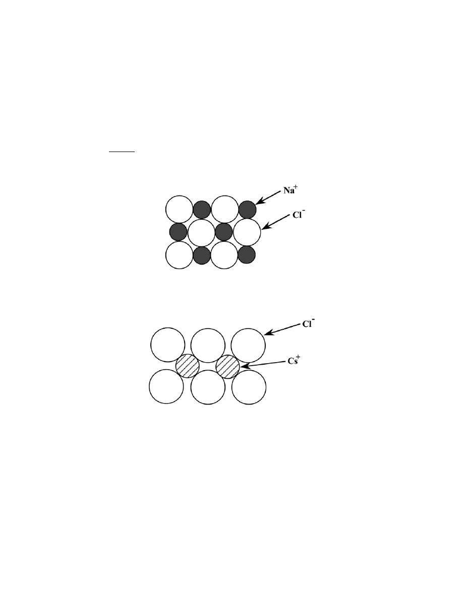
Excerpts from this work may be reproduced by instructors for distribution on a not-for-profit basis for testing or instructional purposes only to
students enrolled in courses for which the textbook has been adopted. Any other reproduction or translation of this work beyond that permitted
by Sections 107 or 108 of the 1976 United States Copyright Act without the permission of the copyright owner is unlawful.
12.25 For each of the following crystal structures, represent the indicated plane in the manner of Figures
3.11 and 3.12, showing both anions and cations:
(a) (100) plane for the rock salt crystal structure,
(b) (110) plane for the cesium chloride crystal structure,
(c) (111) plane for the zinc blende crystal structure, and
(d) (110) plane for the perovskite crystal structure.
Solution
(a) A (100) plane for the rock salt crystal structure would appear as
(b) A (110) plane for the cesium chloride crystal structure would appear as
(c) A (111) plane for the zinc blende crystal structure would appear as
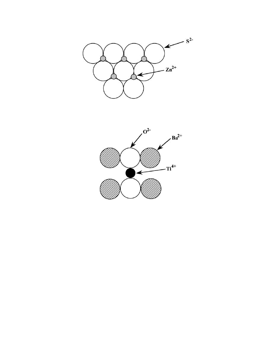
Excerpts from this work may be reproduced by instructors for distribution on a not-for-profit basis for testing or instructional purposes only to
students enrolled in courses for which the textbook has been adopted. Any other reproduction or translation of this work beyond that permitted
by Sections 107 or 108 of the 1976 United States Copyright Act without the permission of the copyright owner is unlawful.
(d) A (110) plane for the perovskite crystal structure would appear as

Excerpts from this work may be reproduced by instructors for distribution on a not-for-profit basis for testing or instructional purposes only to
students enrolled in courses for which the textbook has been adopted. Any other reproduction or translation of this work beyond that permitted
by Sections 107 or 108 of the 1976 United States Copyright Act without the permission of the copyright owner is unlawful.
Silicate Ceramics
12.26 In terms of bonding, explain why silicate materials have relatively low densities.
Solution
The silicate materials have relatively low densities because the atomic bonds are primarily covalent in
nature (Table 12.1), and, therefore, directional. This limits the packing efficiency of the atoms, and therefore, the
magnitude of the density.
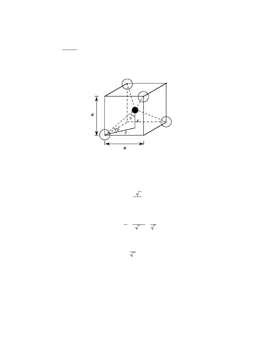
Excerpts from this work may be reproduced by instructors for distribution on a not-for-profit basis for testing or instructional purposes only to
students enrolled in courses for which the textbook has been adopted. Any other reproduction or translation of this work beyond that permitted
by Sections 107 or 108 of the 1976 United States Copyright Act without the permission of the copyright owner is unlawful.
12.27 Determine the angle between covalent bonds in an
SiO
4
4
−
tetrahedron.
Solution
This problem asks for us to determine the angle between covalent bonds in the
SiO
4
4
−
tetrahedron. Below
is shown one such tetrahedron situated within a cube.
Now if we extend the base diagonal from one corner to the other, it is the case that
(2 y)
2
= a
2
+ a
2
= 2a
2
or
y =
a 2
2
Furthermore, x = a/2, and
tan
θ =
x
y
=
a /2
a 2 /2
=
1
2
From which
θ = tan-1
1
2
= 35.26°
Now, solving for the angle
φ
φ = 180° − 90° − 35.26° = 54.74°
Finally, the bond angle is just 2
φ, or 2φ = (2)(54.74°) = 109.48°.

Excerpts from this work may be reproduced by instructors for distribution on a not-for-profit basis for testing or instructional purposes only to
students enrolled in courses for which the textbook has been adopted. Any other reproduction or translation of this work beyond that permitted
by Sections 107 or 108 of the 1976 United States Copyright Act without the permission of the copyright owner is unlawful.
Imperfections in Ceramics
12.28 Would you expect Frenkel defects for anions to exist in ionic ceramics in relatively large
concentrations? Why or why not?
Solution
Frenkel defects for anions would not exist in appreciable concentrations because the anion is quite large
and is highly unlikely to exist as an interstitial.

Excerpts from this work may be reproduced by instructors for distribution on a not-for-profit basis for testing or instructional purposes only to
students enrolled in courses for which the textbook has been adopted. Any other reproduction or translation of this work beyond that permitted
by Sections 107 or 108 of the 1976 United States Copyright Act without the permission of the copyright owner is unlawful.
12.29 Calculate the fraction of lattice sites that are Schottky defects for sodium chloride at its melting
temperature (801°C). Assume an energy for defect formation of 2.3 eV.
Solution
We are asked in this problem to calculate the fraction of lattice sites that are Schottky defects for NaCl at
its melting temperature (801°C), assuming that the energy for defect formation is 2.3 eV. In order to solve this
problem it is necessary to use Equation 12.3 and solve for the N
s
/N ratio. Rearrangement of this expression and
substituting values for the several parameters leads to
N
s
N
= exp
−
Q
s
2kT
= exp
−
2.3 eV
(2)(8.62
×10
-5
eV/K)(801 + 273 K)
= 4.03
× 10
-6

Excerpts from this work may be reproduced by instructors for distribution on a not-for-profit basis for testing or instructional purposes only to
students enrolled in courses for which the textbook has been adopted. Any other reproduction or translation of this work beyond that permitted
by Sections 107 or 108 of the 1976 United States Copyright Act without the permission of the copyright owner is unlawful.
12.30 Calculate the number of Frenkel defects per cubic meter in zinc oxide at 1000°C. The energy for
defect formation is 2.51 eV, while the density for ZnO is 5.55 g/cm
3
at (1000°C).
Solution
This problem asks that we compute the number of Frenkel defects per cubic meter in zinc oxide at 1000
°C.
Solution of this problem is possible using Equation 12.2. However, we must first determine the value of N, the
number of lattice sites per cubic meter, which is possible using a modified form of Equation 4.2; thus
N =
N
A
ρ
A
Zn
+ A
O
=
(6.022
× 10
23
atoms/mol)(5.55 g/cm
3
)(10
6
cm
3
/m
3
)
65.41 g/mol + 16.00 g/mol
= 4.11
× 10
28
lattice sites/m
3
And, finally the value of N
fr
is computed using Equation 12.2 as
N
fr
= N exp
−
Q
fr
2kT
= (4.11
× 10
28
lattice sites/m
3
) exp -
2.51 eV
(2)(8.62
× 10
-5
eV/K)(1000 + 273 K)
= 4.43
× 10
23
defects/m
3

Excerpts from this work may be reproduced by instructors for distribution on a not-for-profit basis for testing or instructional purposes only to
students enrolled in courses for which the textbook has been adopted. Any other reproduction or translation of this work beyond that permitted
by Sections 107 or 108 of the 1976 United States Copyright Act without the permission of the copyright owner is unlawful.
12.31 Using the data given below that relate to the formation of Schottky defects in some oxide ceramic
(having the chemical formula MO), determine the following:
(a) The energy for defect formation (in eV),
(b) The equilibrium number of Schottky defects per cubic meter at 1000°C, and
(c) The identity of the oxide (i.e., what is the metal M?)
T (°C)
ρ (g/cm
3
)
N
s
(m
–3
)
750
5.50
9.21 × 10
19
1000
5.44
?
1250
5.37
5.0 × 10
22
Solution
This problem provides for some oxide ceramic, at temperatures of 750°C and 1250°C, values for density
and the number of Schottky defects per cubic meter. The (a) portion of the problem asks that we compute the
energy for defect formation. To begin, let us combine a modified form of Equation 4.2 and Equation 12.3 as
N
s
= N exp −
Q
s
2kT
=
N
A
ρ
A
M
+ A
O
exp −
Q
s
2kT
Inasmuch as this is a hypothetical oxide material, we don't know the atomic weight of metal M, nor the value of Q
s
in the above equation. Therefore, let us write equations of the above form for two temperatures, T
1
and T
2
. These
are as follows:
N
s1
=
N
A
ρ
1
A
M
+ A
O
exp −
Q
s
2kT
1
(12.S1a)
N
s2
=
N
A
ρ
2
A
M
+ A
O
exp −
Q
s
2kT
2
(12.S1b)
Dividing the first of these equations by the second leads to

Excerpts from this work may be reproduced by instructors for distribution on a not-for-profit basis for testing or instructional purposes only to
students enrolled in courses for which the textbook has been adopted. Any other reproduction or translation of this work beyond that permitted
by Sections 107 or 108 of the 1976 United States Copyright Act without the permission of the copyright owner is unlawful.
N
s1
N
s2
=
N
A
ρ
1
A
M
+ A
O
exp −
Q
s
2kT
1
N
A
ρ
2
A
M
+ A
O
exp −
Q
s
2kT
2
which, after some algebraic manipulation, reduces to the form
N
s1
N
s2
=
ρ
1
ρ
2
exp
−
Q
s
2k
1
T
1
−
1
T
2
(12.S2)
Now, taking natural logarithms of both sides of this equation gives
ln
N
s1
N
s2
= ln
ρ
1
ρ
2
−
Q
s
2k
1
T
1
−
1
T
2
and solving for Q
s
leads to the expression
Q
s
=
−2k ln
N
s1
N
s2
− ln
ρ
1
ρ
2
1
T
1
−
1
T
2
Let us take T
1
= 750°C and T
2
= 1250°C, and we may compute the value of Q
s
as
Q
s
=
−(2)(8.62 × 10
-5
eV/K) ln
9.2
× 10
19
m
-3
5.0
× 10
22
m
-3
− ln
5.50 g/cm
3
5.37 g/cm
3
1
750 + 273 K
−
1
1250 + 273 K
= 3.40 eV
(b) It is now possible to solve for N
s
at 1000°C using Equation 12.S2 above. This time let's take T
1
=
1000°C and T
2
= 750°C. Thus, solving for N
s1
, substituting values provided in the problem statement and Q
s
determined above yields
N
s1
=
N
s2
ρ
1
ρ
2
exp
−
Q
s
2k
1
T
1
−
1
T
2

Excerpts from this work may be reproduced by instructors for distribution on a not-for-profit basis for testing or instructional purposes only to
students enrolled in courses for which the textbook has been adopted. Any other reproduction or translation of this work beyond that permitted
by Sections 107 or 108 of the 1976 United States Copyright Act without the permission of the copyright owner is unlawful.
=
(9.2
× 10
19
m
-3
)( 5.44 g/cm
3
)
5.50 g/cm
3
exp
−
3.40 eV
(2)(8.62
× 10
-5
eV/K)
1
1000 + 273 K
−
1
750 + 273 K
= 4.0 x 10
21
m
-3
(c) And, finally, we want to determine the identity of metal M. This is possible by computing the atomic
weight of M (A
M
) from Equation 12.S1a. Rearrangement of this expression leads to
N
A
ρ
1
A
M
+ A
O
= N
s1
exp
Q
s
2kT
1
And, after further algebraic manipulation
N
A
ρ
1
N
s1
exp
Q
s
2kT
1
= A
M
+ A
O
And, solving this expression for A
M
gives
A
M
=
N
A
ρ
1
N
s1
exp
Q
s
2kT
1
− A
O
Now, assuming that T
1
= 750°C, the value of A
M
is
A
M
=
(6.022
× 10
23
ions/mol)( 5.50 g/cm
3
)(10
6
cm
3
/ m
3
)
(9.2
× 10
19
ions/m
3
) exp
3.40 eV
(2)(8.62
× 10
-5
eV/K)(750 + 273 K)
− 16.00 g/mol
= 136.7 g/mol
Upon consultation of the periodic table in Figure 2.6, the divalent metal (i.e., that forms M
2+
ions) that has an
atomic weight closest to 136.7 g/mol is barium. Thus, this metal oxide is BaO.

Excerpts from this work may be reproduced by instructors for distribution on a not-for-profit basis for testing or instructional purposes only to
students enrolled in courses for which the textbook has been adopted. Any other reproduction or translation of this work beyond that permitted
by Sections 107 or 108 of the 1976 United States Copyright Act without the permission of the copyright owner is unlawful.
12.32 In your own words, briefly define the term “stoichiometric.”
Solution
Stoichiometric means having exactly the ratio of anions to cations as specified by the chemical formula for
the compound.

Excerpts from this work may be reproduced by instructors for distribution on a not-for-profit basis for testing or instructional purposes only to
students enrolled in courses for which the textbook has been adopted. Any other reproduction or translation of this work beyond that permitted
by Sections 107 or 108 of the 1976 United States Copyright Act without the permission of the copyright owner is unlawful.
12.33 If cupric oxide (CuO) is exposed to reducing atmospheres at elevated temperatures, some of the
Cu
2+
ions will become Cu
+
.
(a) Under these conditions, name one crystalline defect that you would expect to form in order to maintain
charge neutrality.
(b) How many Cu
+
ions are required for the creation of each defect?
(c) How would you express the chemical formula for this nonstoichiometric material?
Solution
(a) For a Cu
2+
O
2-
compound in which a small fraction of the copper ions exist as Cu
+
, for each Cu
+
formed there is one less positive charge introduced (or one more negative charge). In order to maintain charge
neutrality, we must either add an additional positive charge or subtract a negative charge. This may be
accomplished be either creating Cu
2+
interstitials or O
2-
vacancies.
(b) There will be two Cu
+
ions required for each of these defects.
(c) The chemical formula for this nonstoichiometric material is Cu
1+x
O or CuO
1-x
, where x is some small
fraction.

Excerpts from this work may be reproduced by instructors for distribution on a not-for-profit basis for testing or instructional purposes only to
students enrolled in courses for which the textbook has been adopted. Any other reproduction or translation of this work beyond that permitted
by Sections 107 or 108 of the 1976 United States Copyright Act without the permission of the copyright owner is unlawful.
12.34 (a) Suppose that Li
2
O is added as an impurity to CaO. If the Li
+
substitutes for Ca
2+
, what kind of
vacancies would you expect to form? How many of these vacancies are created for every Li
+
added?
(b) Suppose that CaCl
2
is added as an impurity to CaO. If the Cl
-
substitutes for O
2-
, what kind of
vacancies would you expect to form? How many of the vacancies are created for every Cl
-
added?
Solution
(a) For Li
+
substituting for Ca
2+
in CaO, oxygen vacancies would be created. For each Li
+
substituting for
Ca
2+
, one positive charge is removed; in order to maintain charge neutrality, a single negative charge may be
removed. Negative charges are eliminated by creating oxygen vacancies, and for every two Li
+
ions added, a single
oxygen vacancy is formed.
(b) For Cl
-
substituting for O
2-
in CaO, calcium vacancies would be created. For each Cl
-
substituting for
an O
2-
, one negative charge is removed; in order to maintain charge neutrality, two Cl
-
ions will lead to the
formation of one calcium vacancy.

Excerpts from this work may be reproduced by instructors for distribution on a not-for-profit basis for testing or instructional purposes only to
students enrolled in courses for which the textbook has been adopted. Any other reproduction or translation of this work beyond that permitted
by Sections 107 or 108 of the 1976 United States Copyright Act without the permission of the copyright owner is unlawful.
12.35 What point defects are possible for Al
2
O
3
as an impurity in MgO? How many Al
3+
ions must be
added to form each of these defects?
Solution
For every Al
3+
ion that substitutes for Mg
2+
in MgO, a single positive charge is added. Thus, in order to
maintain charge neutrality, either a positive charge must be removed or a negative charge must be added.
Negative charges are added by forming O
2-
interstitials, which are not likely to form.
Positive charges may be removed by forming Mg
2+
vacancies, and one magnesium vacancy would be
formed for every two Al
3+
ions added.

Excerpts from this work may be reproduced by instructors for distribution on a not-for-profit basis for testing or instructional purposes only to
students enrolled in courses for which the textbook has been adopted. Any other reproduction or translation of this work beyond that permitted
by Sections 107 or 108 of the 1976 United States Copyright Act without the permission of the copyright owner is unlawful.
Ceramic Phase Diagrams
12.36 For the ZrO
2
–CaO system (Figure 12.26), write all eutectic and eutectoid reactions for cooling.
Solution
There is only one eutectic for the portion of the ZrO
2
-CaO system shown in Figure 12.26. It occurs at
approximately 2250
°C and 23.5 wt% CaO, and, upon cooling, the reaction is
Liquid
→ cubic ZrO
2
+ CaZrO
3
There are two eutectoids. One occurs at about 1000
°C and about 2 wt% CaO; its reaction upon cooling is as
follows:
tetragonal
→ monoclinic ZrO
2
+ cubic ZrO
2
The second eutectoid occurs at about 850
°C and 7 wt% CaO. This reaction is
cubic
→ monoclinic ZrO
2
+ CaZr
4
O
9

Excerpts from this work may be reproduced by instructors for distribution on a not-for-profit basis for testing or instructional purposes only to
students enrolled in courses for which the textbook has been adopted. Any other reproduction or translation of this work beyond that permitted
by Sections 107 or 108 of the 1976 United States Copyright Act without the permission of the copyright owner is unlawful.
12.37 From Figure 12.25, the phase diagram for the MgO–Al
2
O
3
system, it may be noted that the spinel
solid solution exists over a range of compositions, which means that it is nonstoichiometric at compositions other
than 50 mol% MgO–50 mol% Al
2
O
3
.
(a) The maximum nonstoichiometry on the Al
2
O
3
-rich side of the spinel phase field exists at about 2000°C
(3630°F) corresponding to approximately 82 mol% (92 wt%) Al
2
O
3
. Determine the type of vacancy defect that is
produced and the percentage of vacancies that exist at this composition.
(b) The maximum nonstoichiometry on the MgO-rich side of the spinel phase field exists at about 2000°C
(3630°F) corresponding to approximately 39 mol% (62 wt%) Al
2
O
3
. Determine the type of vacancy defect that is
produced and the percentage of vacancies that exist at this composition.
Solution
(a) For this portion of the problem we are to determine the type of vacancy defect that is produced on the
Al
2
O
3
-rich side of the spinel phase field (Figure 12.25) and the percentage of these vacancies at the maximum
nonstoichiometry (82 mol% Al
2
O
3
). On the alumina-rich side of this phase field, there is an excess of Al
3+
ions,
which means that some of the Al
3+
ions substitute for Mg
2+
ions. In order to maintain charge neutrality, Mg
2+
vacancies are formed, and for every Mg
2+
vacancy formed, two Al
3+
ions substitute for three Mg
2+
ions.
Now, we will calculate the percentage of Mg
2+
vacancies that exist at 82 mol% Al
2
O
3
. Let us arbitrarily
choose as our basis 50 MgO-Al
2
O
3
units of the stoichiometric material, which consists of 50 Mg
2+
ions and 100
Al
3+
ions. Furthermore, let us designate the number of Mg
2+
vacancies as x, which means that 2x Al
3+
ions have
been added and 3x Mg
2+
ions have been removed (two of which are filled with Al
3+
ions). Using our 50 MgO-
Al
2
O
3
unit basis, the number of moles of Al
2
O
3
in the nonstoichiometric material is (100 + 2x)/2; similarly the
number of moles of MgO is (50 – 3x). Thus, the expression for the mol% of Al
2
O
3
is just
mol% Al
2
O
3
=
100
+ 2x
2
100
+ 2x
2
+ (50 − 3x)
× 100
If we solve for x when the mol% of Al
2
O
3
= 82, then x = 12.1. Thus, adding 2x or (2)(12.1) = 24.2 Al
3+
ions to the
original material consisting of 100 Al
3+
and 50 Mg
2+
ions will produce 12.1 Mg
2+
vacancies. Therefore, the
percentage of vacancies is just
% vacancies =
12.1
100
+ 50
× 100 = 8.1%

Excerpts from this work may be reproduced by instructors for distribution on a not-for-profit basis for testing or instructional purposes only to
students enrolled in courses for which the textbook has been adopted. Any other reproduction or translation of this work beyond that permitted
by Sections 107 or 108 of the 1976 United States Copyright Act without the permission of the copyright owner is unlawful.
(b) Now, we are asked to make the same determinations for the MgO-rich side of the spinel phase field,
for 39 mol% Al
2
O
3
. In this case, Mg
2+
ions are substituting for Al
3+
ions. Since the Mg
2+
ion has a lower charge
than the Al
3+
ion, in order to maintain charge neutrality, negative charges must be eliminated, which may be
accomplished by introducing O
2-
vacancies. For every 2 Mg
2+
ions that substitute for 2 Al
3+
ions, one O
2-
vacancy is formed.
Now, we will calculate the percentage of O
2-
vacancies that exist at 39 mol% Al
2
O
3
. Let us arbitrarily
choose as our basis 50 MgO-Al2O3 units of the stoichiometric material which consists of 50 Mg
2+
ions 100 Al
3+
ions. Furthermore, let us designate the number of O
2-
vacancies as y, which means that 2y Mg
2+
ions have been
added and 2y Al
3+
ions have been removed. Using our 50 MgO-Al
2
O
3
unit basis, the number of moles of Al
2
O
3
in
the nonstoichiometric material is (100 – 2y)/2; similarly the number of moles of MgO is (50 + 2y). Thus, the
expression for the mol% of Al
2
O
3
is just
mol% Al
2
O
3
=
100
− 2 y
2
100
− 2 y
2
+ (50 + 2 y)
× 100
If we solve for y when the mol% of Al
2
O
3
= 39, then y = 7.91. Thus, 7.91 O
2-
vacancies are produced in the
original material that had 200 O
2-
ions. Therefore, the percentage of vacancies is just
% vacancies =
7.91
200
× 100 = 3.96%

Excerpts from this work may be reproduced by instructors for distribution on a not-for-profit basis for testing or instructional purposes only to
students enrolled in courses for which the textbook has been adopted. Any other reproduction or translation of this work beyond that permitted
by Sections 107 or 108 of the 1976 United States Copyright Act without the permission of the copyright owner is unlawful.
12.38 When kaolinite clay [Al
2
(Si
2
O
5
)(OH)
4
] is heated to a sufficiently high temperature, chemical water
is driven off.
(a) Under these circumstances, what is the composition of the remaining product (in weight percent
Al
2
O
3
)?
(b) What are the liquidus and solidus temperatures of this material
Solution
(a) The chemical formula for kaolinite clay may also be written as Al
2
O
3
–2SiO
2
-2H
2
O. Thus, if we
remove the chemical water, the formula becomes Al
2
O
3
–2SiO
2
. The formula weight for Al
2
O
3
is just (2)(26.98
g/mol) + (3)(16.00 g/mol) = 101.96 g/mol; and for SiO
2
the formula weight is 28.09 g/mol + (2)(16.00 g/mol) =
60.09 g/mol. Thus, the composition of this product, in terms of the concentration of Al
2
O
3
, C
Al
2
O
3
, in weight
percent is just
C
Al
2
O
3
=
101.96 g / mol
101.96 g / mol
+ (2)(60.09 g /mol)
× 100 = 45.9 wt%
(b) The liquidus and solidus temperatures for this material as determined from the SiO
2
–Al
2
O
3
phase
diagram, Figure 12.27, are 1825
°C and 1587°C, respectively.

Excerpts from this work may be reproduced by instructors for distribution on a not-for-profit basis for testing or instructional purposes only to
students enrolled in courses for which the textbook has been adopted. Any other reproduction or translation of this work beyond that permitted
by Sections 107 or 108 of the 1976 United States Copyright Act without the permission of the copyright owner is unlawful.
Brittle Fracture of Ceramics
12.39 Briefly explain
(a) why there may be significant scatter in the fracture strength for some given ceramic material, and
(b) why fracture strength increases with decreasing specimen size.
Solution
(a) There may be significant scatter in the fracture strength for some given ceramic material because the
fracture strength depends on the probability of the existence of a flaw that is capable of initiating a crack; this
probability varies from specimen to specimen of the same material.
(b) The fracture strength increases with decreasing specimen size because as specimen size decreases, the
probably of the existence of a flaw of that is capable of initiating a crack diminishes.

Excerpts from this work may be reproduced by instructors for distribution on a not-for-profit basis for testing or instructional purposes only to
students enrolled in courses for which the textbook has been adopted. Any other reproduction or translation of this work beyond that permitted
by Sections 107 or 108 of the 1976 United States Copyright Act without the permission of the copyright owner is unlawful.
12.40 The tensile strength of brittle materials may be determined using a variation of Equation 8.1.
Compute the critical crack tip radius for an Al
2
O
3
specimen that experiences tensile fracture at an applied stress of
275 MPa (40,000 psi). Assume a critical surface crack length of 2
× 10
-3
mm and a theoretical fracture strength of
E/10, where E is the modulus of elasticity.
Solution
We are asked for the critical crack tip radius for an Al
2
O
3
material. From Equation 8.1
σ
m
= 2
σ
0
a
ρ
t
1/ 2
Fracture will occur when
σ
m
reaches the fracture strength of the material, which is given as E/10; thus
E
10
= 2
σ
0
a
ρ
t
1/ 2
Or, solving for
ρ
t
ρ
t
=
400 a
σ
0
2
E
2
From Table 12.5, E = 393 GPa, and thus,
ρ
t
=
(400 )
(
2
× 10
−3
mm
)
(275 MPa)
2
(
393
× 10
3
MPa
)
2
= 3.9
× 10
-7
mm = 0.39 nm

Excerpts from this work may be reproduced by instructors for distribution on a not-for-profit basis for testing or instructional purposes only to
students enrolled in courses for which the textbook has been adopted. Any other reproduction or translation of this work beyond that permitted
by Sections 107 or 108 of the 1976 United States Copyright Act without the permission of the copyright owner is unlawful.
12.41 The fracture strength of glass may be increased by etching away a thin surface layer. It is believed
that the etching may alter surface crack geometry (i.e., reduce crack length and increase the tip radius). Compute
the ratio of the original and etched crack tip radii for an eightfold increase in fracture strength if two-thirds of the
crack length is removed.
Solution
This problem asks that we compute the crack tip radius ratio before and after etching. Let
ρ
t
= original crack tip radius, and
ρ
t
' = etched crack tip radius
Also,
σ
f
' =
σ
f
a ' =
a
3
σ
0
' = 8
σ
0
Solving for
ρ
t
'
ρ
t
from the following
σ
f
= 2
σ
0
a
ρ
t
1/2
=
σ
f
' = 2
σ
0
' a
'
ρ
t
'
1/2
yields
ρ
t
'
ρ
t
=
σ
0
'
σ
0
2
a
'
a
=
8
σ
0
σ
0
2
a/ 3
a
= 21.3

Excerpts from this work may be reproduced by instructors for distribution on a not-for-profit basis for testing or instructional purposes only to
students enrolled in courses for which the textbook has been adopted. Any other reproduction or translation of this work beyond that permitted
by Sections 107 or 108 of the 1976 United States Copyright Act without the permission of the copyright owner is unlawful.
Stress-Strain Behavior
12.42 A three-point bending test is performed on a glass specimen having a rectangular cross section of
height d = 5 mm (0.2 in.) and width b = 10 mm (0.4 in.); the distance between support points is 45 mm (1.75 in.).
(a) Compute the flexural strength if the load at fracture is 290 N (65 lb
f
).
(b)
The point of maximum deflection Δy occurs at the center of the specimen and is described by
∆y =
FL
3
48EI
where E is the modulus of elasticity and I is the cross-sectional moment of inertia. Compute
∆y at a load of 266 N
(60 lb
f
).
Solution
(a) For this portion of the problem we are asked to compute the flexural strength for a glass specimen that
is subjected to a three-point bending test. The flexural strength (Equation 12.7a) is just
σ
fs
=
3F
f
L
2bd
2
for a rectangular cross-section. Using the values given in the problem statement,
σ
fs
=
(3)(290 N)
(
45
× 10
−3
m
)
(2)
(
10
× 10
−3
m
)
(
5
× 10
−3
m
)
2
= 7.83
× 10
7
N/m
2
= 78.3 MPa (10, 660 psi)
(b) We are now asked to compute the maximum deflection. From Table 12.5, the elastic modulus (E) for
glass is 69 GPa (10
× 10
6
psi). Also, the moment of inertia for a rectangular cross section (Figure 12.32) is just
I =
bd
3
12
Thus,
∆y =
FL
3
48E
bd
3
12
=
FL
3
4Ebd
3

Excerpts from this work may be reproduced by instructors for distribution on a not-for-profit basis for testing or instructional purposes only to
students enrolled in courses for which the textbook has been adopted. Any other reproduction or translation of this work beyond that permitted
by Sections 107 or 108 of the 1976 United States Copyright Act without the permission of the copyright owner is unlawful.
=
(266 N)
(
45
× 10
−3
m
)
3
(4)
(
69
× 10
9
N/m
2
)(
10
× 10
−3
m
)
(
5
× 10
−3
m
)
3
= 7.0
× 10
-5
m = 7.0
× 10
-2
mm
(
2.5
× 10
-3
in.
)

Excerpts from this work may be reproduced by instructors for distribution on a not-for-profit basis for testing or instructional purposes only to
students enrolled in courses for which the textbook has been adopted. Any other reproduction or translation of this work beyond that permitted
by Sections 107 or 108 of the 1976 United States Copyright Act without the permission of the copyright owner is unlawful.
12.43 A circular specimen of MgO is loaded using a three-point bending mode. Compute the minimum
possible radius of the specimen without fracture, given that the applied load is 425 N (95.5 lb
f
), the flexural
strength is 105 MPa (15,000 psi), and the separation between load points is 50 mm (2.0 in.).
Solution
We are asked to calculate the maximum radius of a circular specimen of MgO that is loaded using three-
point bending. Solving for R from Equation 12.7b
R =
F
f
L
σ
fs
π
1/3
which, when substituting the parameters stipulated in the problem statement, yields
R =
(425 N)
(
50
× 10
−3
m
)
(
105
× 10
6
N / m
2
)
(
π)
1/3
= 4.0
× 10
-3
m = 4.0 mm (0.16 in.)

Excerpts from this work may be reproduced by instructors for distribution on a not-for-profit basis for testing or instructional purposes only to
students enrolled in courses for which the textbook has been adopted. Any other reproduction or translation of this work beyond that permitted
by Sections 107 or 108 of the 1976 United States Copyright Act without the permission of the copyright owner is unlawful.
12.44 A three-point bending test was performed on an aluminum oxide specimen having a circular cross
section of radius 3.5 mm (0.14 in.); the specimen fractured at a load of 950 N (215 lb
f
) when the distance between
the support points was 50 mm (2.0 in.). Another test is to be performed on a specimen of this same material, but
one that has a square cross section of 12 mm (0.47 in.) length on each edge. At what load would you expect this
specimen to fracture if the support point separation is 40 mm (1.6 in.)?
Solution
For this problem, the load is given at which a circular specimen of aluminum oxide fractures when
subjected to a three-point bending test; we are then are asked to determine the load at which a specimen of the same
material having a square cross-section fractures. It is first necessary to compute the flexural strength of the
aluminum oxide, Equation 12.7b, and then, using this value, we may calculate the value of F
f
in Equation 12.7a.
From Equation 12.7b
σ
fs
=
F
f
L
πR
3
=
(950 N)
(
50
× 10
−3
m
)
(
π)
(
3.5
× 10
−3
m
)
3
= 352
× 10
6
N/m
2
= 352 MPa (50, 000 psi)
Now, solving for F
f
from Equation 12.7a, realizing that b = d = 12 mm, yields
F
f
=
2
σ
fs
d
3
3L
=
(2)
(
352
× 10
6
N / m
2
)
(
12
× 10
−3
m
)
3
(3)
(
40
× 10
−3
m
)
= 10,100 N (2165 lb
f
)

Excerpts from this work may be reproduced by instructors for distribution on a not-for-profit basis for testing or instructional purposes only to
students enrolled in courses for which the textbook has been adopted. Any other reproduction or translation of this work beyond that permitted
by Sections 107 or 108 of the 1976 United States Copyright Act without the permission of the copyright owner is unlawful.
12.45 (a) A three-point transverse bending test is conducted on a cylindrical specimen of aluminum oxide
having a reported flexural strength of 390 MPa (56,600 psi). If the specimen radius is 2.5 mm (0.10 in.) and the
support point separation distance is 30 mm (1.2 in.), predict whether or not you would expect the specimen to
fracture when a load of 620 N (140 lb
f
) is applied. Justify your prediction.
(b) Would you be 100% certain of the prediction in part (a)? Why or why not?
Solution
(a) This portion of the problem asks that we determine whether or not a cylindrical specimen of aluminum
oxide having a flexural strength of 390 MPa (56,600 psi) and a radius of 2.5 mm will fracture when subjected to a
load of 620 N in a three-point bending test; the support point separation is given as 30 mm. Using Equation 12.7b
we will calculate the value of
σ; if this value is greater than σ
fs
(390 MPa), then fracture is expected to occur.
Employment of Equation 12.7b yields
σ =
FL
πR
3
=
(620 N)
(
30
× 10
−3
m
)
(
π)
(
2.5
× 10
−3
m
)
3
= 379
× 10
6
N/m
2
= 379 MPa (53,500 psi)
Since this value is less than the given value of
σ
fs
(390 MPa), then fracture is not predicted.
(b) The certainty of this prediction is not 100% because there is always some variability in the flexural
strength for ceramic materials, and since this value of
σ (379 MPa) is relatively close to σ
fs
(390 MPa) then there is
some chance that fracture will occur.

Excerpts from this work may be reproduced by instructors for distribution on a not-for-profit basis for testing or instructional purposes only to
students enrolled in courses for which the textbook has been adopted. Any other reproduction or translation of this work beyond that permitted
by Sections 107 or 108 of the 1976 United States Copyright Act without the permission of the copyright owner is unlawful.
Mechanisms of Plastic Deformation
12.46 Cite one reason why ceramic materials are, in general, harder yet more brittle than metals.
Solution
Crystalline ceramics are harder yet more brittle than metals because they (ceramics) have fewer slip
systems, and, therefore, dislocation motion is highly restricted.

Excerpts from this work may be reproduced by instructors for distribution on a not-for-profit basis for testing or instructional purposes only to
students enrolled in courses for which the textbook has been adopted. Any other reproduction or translation of this work beyond that permitted
by Sections 107 or 108 of the 1976 United States Copyright Act without the permission of the copyright owner is unlawful.
Miscellaneous Mechanical Considerations
12.47 The modulus of elasticity for beryllium oxide (BeO) having 5 vol% porosity is 310 GPa (45
× 10
6
psi).
(a) Compute the modulus of elasticity for the nonporous material.
(b) Compute the modulus of elasticity for 10 vol% porosity.
Solution
(a) This portion of the problem requests that we compute the modulus of elasticity for nonporous BeO
given that E = 310 GPa for a material having 5 vol% porosity. Thus, we solve Equation 12.9 for E
0
, using P = 0.05,
which gives
E
0
=
E
1
− 1.9P + 0.9P
2
=
310 GPa
1
− (1.9)(0.05) + (0.9)(0.05)
2
= 342 GPa
(
49.6
× 10
6
psi
)
(b) Now we are asked to determine the value of E at P = 10 vol% (i.e., 0.10). Using Equation 12.9 we get
E = E
0
(
1
− 1.9P + 0.9P
2
)
= (342 GPa) 1
− (1.9)(0.10) + (0.9)(0.10)
2
[
]
= 280 GPa
(
40.6
× 10
6
psi
)
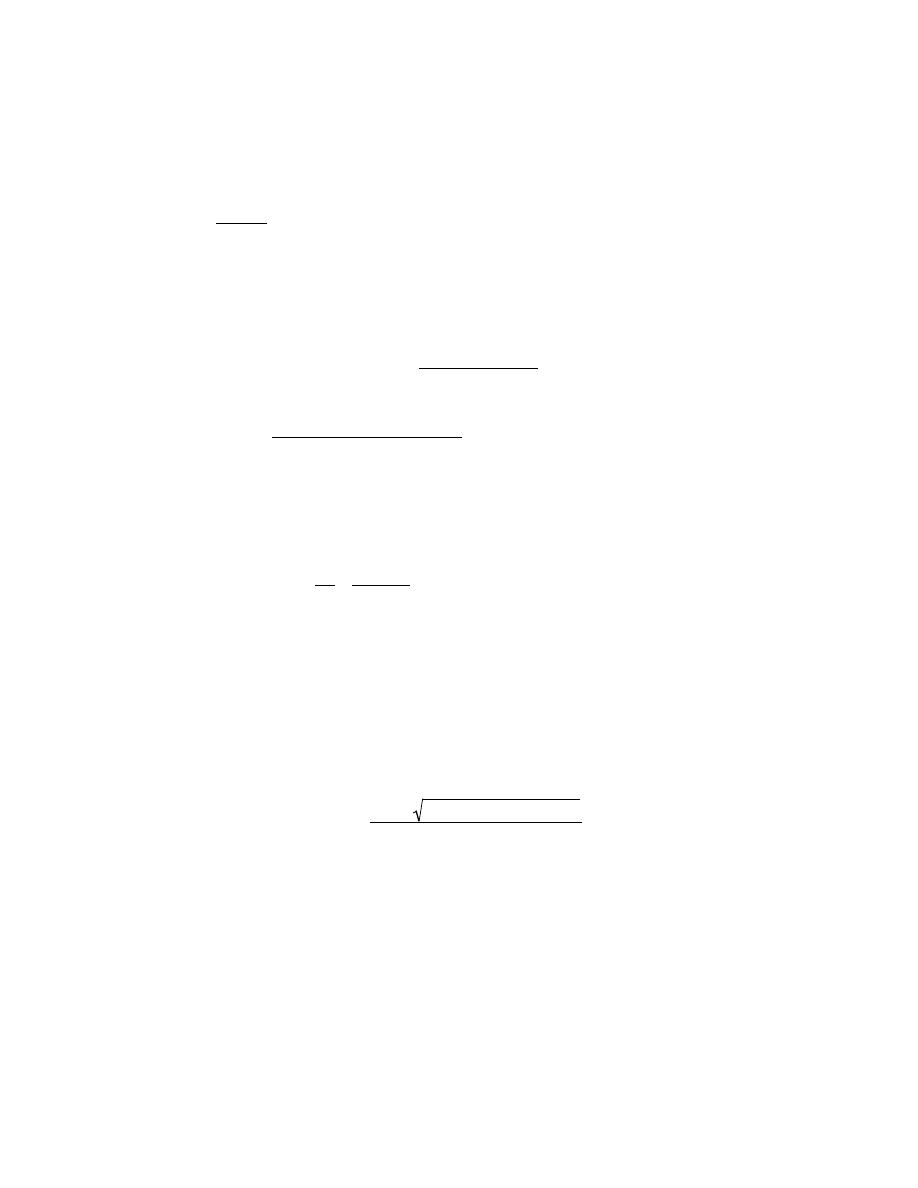
Excerpts from this work may be reproduced by instructors for distribution on a not-for-profit basis for testing or instructional purposes only to
students enrolled in courses for which the textbook has been adopted. Any other reproduction or translation of this work beyond that permitted
by Sections 107 or 108 of the 1976 United States Copyright Act without the permission of the copyright owner is unlawful.
12.48 The modulus of elasticity for boron carbide (B
4
C) having 5 vol% porosity is 290 GPa (42
× 10
6
psi).
(a) Compute the modulus of elasticity for the nonporous material.
(b) At what volume percent porosity will the modulus of elasticity be 235 GPa (34
× 10
6
psi)?
Solution
(a) This portion of the problem requests that we compute the modulus of elasticity for nonporous B
4
C
given that E = 290 GPa (42
× 10
6
psi) for a material having 5 vol% porosity. Thus, we solve Equation 12.9 for E
0
,
using P = 0.05, which gives
E
0
=
E
1
− 1.9P + 0.9P
2
=
290 GPa
1
− (1.9)(0.05) + (0.9)(0.05)
2
= 320 GPa
(
46.3
× 10
6
psi
)
(b) Now we are asked to compute the volume percent porosity at which the elastic modulus of B
4
C is 235
MPa (34
× 10
6
psi). Since from part (a), E
0
= 320 GPa, and using Equation 12.9 we get
E
E
0
=
235 MPa
320 MPa
= 0.734 = 1
− 1.9P + 0.9P
2
Or
0.9P
2
− 1.9P + 0.266 = 0
Now, solving for the value of P using the quadratic equation solution yields
P =
1.9
±
(
−1.9)
2
− (4)(0.9)(0.266)
(2)(0.9)
The positive and negative roots are
P
+
= 1.96
P
-
= 0.151
Obviously, only the negative root is physically meaningful, and therefore the value of the porosity to give the
desired modulus of elasticity is 15.1 vol%.

Excerpts from this work may be reproduced by instructors for distribution on a not-for-profit basis for testing or instructional purposes only to
students enrolled in courses for which the textbook has been adopted. Any other reproduction or translation of this work beyond that permitted
by Sections 107 or 108 of the 1976 United States Copyright Act without the permission of the copyright owner is unlawful.
12.49 Using the data in Table 12.5, do the following:
(a) Determine the flexural strength for nonporous MgO assuming a value of 3.75 for n in Equation 12.10.
(b) Compute the volume fraction porosity at which the flexural strength for MgO is 62 MPa (9000 psi).
Solution
(a) This part of the problem asks us to determine the flexural strength of nonporous MgO assuming that
the value of n in Equation 12.10 is 3.75. Taking natural logarithms of both sides of Equation 12.10 yields
ln
σ
fs
= ln
σ
0
− nP
In Table 12.5 it is noted that for P = 0.05,
σ
fs
= 105 MPa. For the nonporous material P = 0 and, ln
σ
0
= ln
σ
f
ff
s
ss
.
Solving for ln
σ
0
from the above equation and using these data gives
ln
σ
0
= ln
σ
fs
+ nP
= ln (105 MPa) + (3.75)(0.05) = 4.841
or
σ
0
= e
4.841
= 127 MPa (18,100 psi)
(b) Now we are asked to compute the volume percent porosity to yield a
σ
fs
of 62 MPa (9000 psi). Taking
the natural logarithm of Equation 12.10 and solving for P leads to
P =
ln
σ
0
− ln σ
fs
n
=
ln (127 MPa)
− ln (62 MPa)
3.75
= 0.19 or 19 vol%

Excerpts from this work may be reproduced by instructors for distribution on a not-for-profit basis for testing or instructional purposes only to
students enrolled in courses for which the textbook has been adopted. Any other reproduction or translation of this work beyond that permitted
by Sections 107 or 108 of the 1976 United States Copyright Act without the permission of the copyright owner is unlawful.
12.50 The flexural strength and associated volume fraction porosity for two specimens of the same ceramic
material are as follows:
σ
fs
(MPa)
P
100
0.05
50
0.20
(a) Compute the flexural strength for a completely nonporous specimen of this material.
(b) Compute the flexural strength for a 0.10 volume fraction porosity.
Solution
(a) Given the flexural strengths at two different volume fraction porosities, we are asked to determine the
flexural strength for a nonporous material. If the natural logarithm is taken of both sides of Equation 12.10, then
ln
σ
fs
= ln
σ
0
− nP
Using the data provided in the problem statement, two simultaneous equations may be written as
ln (100 MPa) = ln
σ
0
− (0.05) n
ln (50 MPa) = ln
σ
0
− (0.20) n
Solving for n and
σ
0
leads to n = 4.62 and
σ
0
= 126 MPa. For the nonporous material, P = 0, and, from Equation
12.10,
σ
0
=
σ
fs
. Thus,
σ
fs
for P = 0 is 126 MPa.
(b) Now, we are asked for
σ
fs
at P = 0.10 for this same material. Utilizing Equation 12.10 yields
σ
fs
=
σ
0
exp (
− nP)
= (126 MPa) exp
− (4.62)(0.10)
[
]
= 79.4 MPa

Excerpts from this work may be reproduced by instructors for distribution on a not-for-profit basis for testing or instructional purposes only to
students enrolled in courses for which the textbook has been adopted. Any other reproduction or translation of this work beyond that permitted
by Sections 107 or 108 of the 1976 United States Copyright Act without the permission of the copyright owner is unlawful.
DESIGN PROBLEMS
Crystal Structures
12.D1 Gallium arsenide (GaAs) and gallium phosphide (GaP) both have the zinc blende crystal structure
and are soluble in one another at all concentrations. Determine the concentration in weight percent of GaP that
must be added to GaAs to yield a unit cell edge length of 0.5570 nm. The densities of GaAs and GaP are 5.316 and
4.130 g/cm
3
, respectively.
Solution
This problem asks that we determine the concentration (in weight percent) of GaP that must be added to
GaAs to yield a unit cell edge length of 0.5570 nm. The densities of GaAs and GaP were given in the problem as
5.307 and 4.130 g/cm
3
, respectively. To begin, it is necessary to employ Equation (13.1), and solve for the unit cell
volume, V
C
, for the GaP-GaAs alloy as
V
C
=
n' A
ave
ρ
ave
N
A
where A
ave
and
ρ
ave
are the atomic weight and density, respectively, of the InAs-GaAs alloy. Inasmuch as both of
these materials have the zinc blende crystal structure, which has cubic symmetry, V
C
is just the cube of the unit cell
length, a. That is
V
C
= a
3
= (0.5570 nm)
3
=
(
5.570
× 10
−8
cm
)
3
= 1.728 × 10
−22
cm
3
It is now necessary to construct expressions for A
ave
and
ρ
ave
in terms of the concentration of indium arsenide,
C
InAs
using Equations 4.11a and 4.10a. For A
ave
we have
A
ave
=
100
C
GaP
A
GaP
+
(
100
− C
GaP
)
A
GaAs
=
100
C
GaP
100.69 g/mol
+
(
100
− C
GaP
)
144.64 g/mol

Excerpts from this work may be reproduced by instructors for distribution on a not-for-profit basis for testing or instructional purposes only to
students enrolled in courses for which the textbook has been adopted. Any other reproduction or translation of this work beyond that permitted
by Sections 107 or 108 of the 1976 United States Copyright Act without the permission of the copyright owner is unlawful.
whereas for
ρ
ave
ρ
ave
=
100
C
GaP
ρ
GaP
+
(
100
− C
GaP
)
ρ
GaAs
=
100
C
GaP
4.130 g/cm
3
+
(
100
− C
GaP
)
5.316 g/cm
3
Within the zinc blende unit cell there are four formula units, and thus, the value of n' in Equation 12.1 is 4; hence,
this expression may be written in terms of the concentration of GaP in weight percent as follows:
V
C
= 1.728
× 10
-22
cm
3
=
n' A
ave
ρ
ave
N
A
=
(4 formula units/unit cell)
100
C
GaP
100.69 g/mol
+
(
100
− C
GaP
)
144.64 g/mol
100
C
GaP
4.130 g/cm
3
+
(
100
− C
GaP
)
5.316 g/cm
3
(
6.022
× 10
23
formula units/mol
)
And solving this expression for C
GaP
leads to C
GaP
= 33.7 wt%.

Excerpts from this work may be reproduced by instructors for distribution on a not-for-profit basis for testing or instructional purposes only to
students enrolled in courses for which the textbook has been adopted. Any other reproduction or translation of this work beyond that permitted
by Sections 107 or 108 of the 1976 United States Copyright Act without the permission of the copyright owner is unlawful.
Stress-Strain Behavior
12.D2 It is necessary to select a ceramic material to be stressed using a three-point loading scheme
(Figure 12.32). The specimen must have a circular cross section and a radius of 2.5 mm (0.10 in.), and must not
experience fracture or a deflection of more than 6.2
× 10
-2
mm (2.4
× 10
-3
in.) at its center when a load of 275 N (62
lb
f
) is applied. If the distance between support points is 45 mm (1.77 in.), which of the materials in Table 12.5 are
candidates? The magnitude of the centerpoint deflection may be computed using the equation supplied in Problem
12.42.
Solution
This problem asks for us to determine which of the ceramic materials in Table 12.5, when fabricated into
cylindrical specimens and stressed in three-point loading, will not fracture when a load of 275 N (62 lb
f
) is applied,
and also will not experience a center-point deflection of more than 6.2
× 10
-2
mm (2.4
× 10
-3
in.). The first of these
criteria is met by those materials that have flexural strengths greater than the stress calculated using Equation 12.7b.
According to this expression
σ
fs
=
FL
π R
3
=
(275 N)
(
45
× 10
−3
m
)
(
π)
(
2.5
× 10
−3
m
)
3
= 252 × 10
6
N / m
2
= 252 MPa (35,000 psi)
Of the materials in Table 12.5, the following have flexural strengths greater than this value: Si
3
N
4
, ZrO
2
, SiC, and
Al
2
O
3
For the second criterion we must solve for the magnitude of the modulus of elasticity, E, from the equation
given in Problem 12.42 where the expression for the cross-sectional moment of inertia appears in Figure 12.32; that
is, for a circular cross-section
I =
π R
4
4
. Solving for E from these two expressions
E =
FL
3
12
π R
4
∆y
=
(275 N)
(
45
× 10
−3
m
)
3
(12)(
π)
(
2.5
× 10
−3
m
)
4
(
6.2
× 10
−5
m
)
= 274
× 10
9
N/m
2
= 274 GPa (38
× 10
6
psi)

Excerpts from this work may be reproduced by instructors for distribution on a not-for-profit basis for testing or instructional purposes only to
students enrolled in courses for which the textbook has been adopted. Any other reproduction or translation of this work beyond that permitted
by Sections 107 or 108 of the 1976 United States Copyright Act without the permission of the copyright owner is unlawful.
Of those materials that satisfy the first criterion, only Al
2
O
3
, Si
3
N
4
, and SiC have moduli of elasticity greater than
this value (Table 12.5), and, therefore, are possible candidates.

Excerpts from this work may be reproduced by instructors for distribution on a not-for-profit basis for testing or instructional purposes only to
students enrolled in courses for which the textbook has been adopted. Any other reproduction or translation of this work beyond that permitted
by Sections 107 or 108 of the 1976 United States Copyright Act without the permission of the copyright owner is unlawful.
CHAPTER 13
APPLICATIONS AND PROCESSING OF CERAMICS
PROBLEM SOLUTIONS
Glasses
Glass-Ceramics
13.1 Cite the two desirable characteristics of glasses.
Solution
Two desirable characteristics of glasses are optical transparency and ease of fabrication.

Excerpts from this work may be reproduced by instructors for distribution on a not-for-profit basis for testing or instructional purposes only to
students enrolled in courses for which the textbook has been adopted. Any other reproduction or translation of this work beyond that permitted
by Sections 107 or 108 of the 1976 United States Copyright Act without the permission of the copyright owner is unlawful.
13.2 (a) What is crystallization?
(b) Cite two properties that may be improved by crystallization.
Solution
(a) Crystallization is the process whereby a glass material is caused to transform to a crystalline solid,
usually as a result of a heat treatment.
(b) Two properties that may be improved by crystallization are (1) a lower coefficient of thermal
expansion, and (2) higher strength.

Excerpts from this work may be reproduced by instructors for distribution on a not-for-profit basis for testing or instructional purposes only to
students enrolled in courses for which the textbook has been adopted. Any other reproduction or translation of this work beyond that permitted
by Sections 107 or 108 of the 1976 United States Copyright Act without the permission of the copyright owner is unlawful.
Refractories
13.3 For refractory ceramic materials, cite three characteristics that improve with and two characteristics
that are adversely affected by increasing porosity.
Solution
For refractory ceramic materials, three characteristics that improve with increasing porosity are (1)
decreased thermal expansion and contraction upon thermal cycling, (2) improved thermal insulation, and (3)
improved resistance to thermal shock. Two characteristics that are adversely affected are (1) load-bearing capacity
and (2) resistance to attack by corrosive materials.

Excerpts from this work may be reproduced by instructors for distribution on a not-for-profit basis for testing or instructional purposes only to
students enrolled in courses for which the textbook has been adopted. Any other reproduction or translation of this work beyond that permitted
by Sections 107 or 108 of the 1976 United States Copyright Act without the permission of the copyright owner is unlawful.
13.4 Find the maximum temperature to which the following two magnesia–alumina refractory materials
may be heated before a liquid phase will appear.
(a) A spinel-bonded alumina material of composition 95 wt% Al
2
O
3
-5 wt% MgO.
(b) A magnesia-alumina spinel of composition 65 wt% Al
2
O
3
-35 wt% MgO.
Consult Figure 12.25.
Solution
(a) From Figure 12.25, for a spinel-bonded magnesia material (95 wt% Al
2
O
3
-5 wt% MgO), the maximum
temperature without a liquid phase corresponds to the temperature of the eutectic isotherm on the Al
2
O
3
-rich side of
the phase diagram, which is approximately 2000
°C (3630°F).
(b) The maximum temperature without the formation of a liquid phase for a magnesia-alumina spinel (65
wt% Al
2
O
3
-35 wt% MgO) lies at the phase boundary between MgAl
2
O
4
(ss)-MgAl
2
O
4
+ Liquid phase fields (just
slightly to the left of the congruent melting point at which the two phase boundaries become tangent); this
temperature is approximately 2030
°C (3685°F).

Excerpts from this work may be reproduced by instructors for distribution on a not-for-profit basis for testing or instructional purposes only to
students enrolled in courses for which the textbook has been adopted. Any other reproduction or translation of this work beyond that permitted
by Sections 107 or 108 of the 1976 United States Copyright Act without the permission of the copyright owner is unlawful.
13.5 Upon consideration of the SiO
2
–Al
2
O
3
phase diagram, Figure 12.27, for each pair of the following
list of compositions, which would you judge to be the more desirable refractory? Justify your choices.
(a) 20 wt% Al
2
O
3
-80 wt% SiO
2
and 25 wt% Al
2
O
3
-75 wt% SiO
2
(b) 70 wt% Al
2
O
3
-30 wt% SiO
2
and 80 wt% Al
2
O
3
-20 wt% SiO
2
Solution
(a) The 25 wt% Al
2
O
3
-75 wt% SiO
2
will be more desirable because the liquidus temperature will be
greater for this composition; therefore, at any temperature within the mullite + liquid region on the phase diagram,
there will be a lower fraction of the liquid phase present than for the 20 wt% Al
2
O
3
-80 wt% SiO
2
composition, and,
thus, the mechanical integrity will be greater.
(b) The 80 wt% Al
2
O
3
-20 wt% SiO
2
composition will be more desirable because, for this composition, a
liquid phase does not form until about 1890
°C, whereas, for the 70 wt% Al
2
O
3
-30 wt% SiO
2
material, a liquid
phase forms at a much lower temperature--1587
°C.

Excerpts from this work may be reproduced by instructors for distribution on a not-for-profit basis for testing or instructional purposes only to
students enrolled in courses for which the textbook has been adopted. Any other reproduction or translation of this work beyond that permitted
by Sections 107 or 108 of the 1976 United States Copyright Act without the permission of the copyright owner is unlawful.
13.6 Compute the mass fractions of liquid in the following refractory materials at 1600°C (2910°F):
(a) 6 wt% Al
2
O
3
-94 wt% SiO
2
(b) 10 wt% Al
2
O
3
-90 wt% SiO
2
(c) 30 wt% Al
2
O
3
-70 wt% SiO
2
(d) 80 wt% Al
2
O
3
-20 wt% SiO
2
Solution
This problem calls for us to compute the mass fractions of liquid for two fireclay refractory materials at
1600
°C. In order to solve this problem it is necessary that we use the SiO
2
-Al
2
O
3
phase diagram (Figure 12.27) in
conjunction with tie-lines and the lever rule at 1600
°C.
(a) For the 6 wt% Al
2
O
3
-94 wt% SiO
2
composition, the appropriate lever-rule expression is
W
L
=
C
0
− C
SiO
2
C
L
− C
SiO
2
For a tie-line constructed across the SiO
2
-Liquid phase field at 1600
°C
C
L
= 7 wt% Al
2
O
3
C
SiO2
= 0 wt% Al
2
O
3
And, inasmuch as C
0
= 6 wt% Al
2
O
3
the mass fraction of liquid using the above lever-rule expression is
W
L
=
6
− 0
7
− 0
= 0.86
(b) For the 10 wt% Al
2
O
3
-90 wt% SiO
2
composition, the appropriate lever-rule expression is
W
L
=
C
mullite
− C
0
C
mullite
− C
L
For a tie-line constructed across the Mullite (ss)-Liquid phase field at 1600
°C
C
mullite
= 72 wt% Al
2
O
3
C
L
= 8 wt% Al
2
O
3
And, inasmuch as C
0
= 10 wt% Al
2
O
3
the mass fraction of liquid using the above lever-rule expression is
W
L
=
72
− 10
72
− 8
= 0.97

Excerpts from this work may be reproduced by instructors for distribution on a not-for-profit basis for testing or instructional purposes only to
students enrolled in courses for which the textbook has been adopted. Any other reproduction or translation of this work beyond that permitted
by Sections 107 or 108 of the 1976 United States Copyright Act without the permission of the copyright owner is unlawful.
(c) For the 30 wt% Al
2
O
3
-70 wt% SiO
2
composition, the appropriate lever-rule expression is
W
L
=
C
mullite
− C
0
C
mullite
− C
L
For a tie-line constructed across the Mullite (ss)-Liquid phase field at 1600
°C
C
mullite
= 72 wt% Al
2
O
3
C
L
= 8 wt% Al
2
O
3
And, inasmuch as C
0
= 30 wt% Al
2
O
3
the mass fraction of liquid using the above lever-rule expression is
W
L
=
72
− 30
72
− 8
= 0.66
(d) For the 80 wt% Al
2
O
3
-20 wt% SiO
2
composition at 1600
°C, only alumina and mullite phases are
present; thus W
L
= 0.

Excerpts from this work may be reproduced by instructors for distribution on a not-for-profit basis for testing or instructional purposes only to
students enrolled in courses for which the textbook has been adopted. Any other reproduction or translation of this work beyond that permitted
by Sections 107 or 108 of the 1976 United States Copyright Act without the permission of the copyright owner is unlawful.
13.7 For the MgO–Al
2
O
3
system, what is the maximum temperature that is possible without the formation
of a liquid phase? At what composition or over what range of compositions will this maximum temperature be
achieved?
Solution
This problem asks that we specify, for the MgO-Al
2
O
3
system, Figure 12.25, the maximum temperature
without the formation of a liquid phase; it is approximately 2800
°C which is possible for pure MgO.

Excerpts from this work may be reproduced by instructors for distribution on a not-for-profit basis for testing or instructional purposes only to
students enrolled in courses for which the textbook has been adopted. Any other reproduction or translation of this work beyond that permitted
by Sections 107 or 108 of the 1976 United States Copyright Act without the permission of the copyright owner is unlawful.
Cements
13.8 Compare the manner in which the aggregate particles become bonded together in clay-based
mixtures during firing and in cements during setting.
Solution
For clay-based aggregates, a liquid phase forms during firing, which infiltrates the pores between the
unmelted particles; upon cooling, this liquid becomes a glass, that serves as the bonding phase.
With cements, the bonding process is a chemical, hydration reaction between the water that has been added
and the various cement constituents. The cement particles are bonded together by reactions that occur at the particle
surfaces.

Excerpts from this work may be reproduced by instructors for distribution on a not-for-profit basis for testing or instructional purposes only to
students enrolled in courses for which the textbook has been adopted. Any other reproduction or translation of this work beyond that permitted
by Sections 107 or 108 of the 1976 United States Copyright Act without the permission of the copyright owner is unlawful.
Fabrication and Processing of Glasses and Glass-Ceramics
13.9 Soda and lime are added to a glass batch in the form of soda ash (Na
2
CO
3
) and limestone (CaCO
3
).
During heating, these two ingredients decompose to give off carbon dioxide (CO
2
), the resulting products being
soda and lime. Compute the weight of soda ash and limestone that must be added to 100 lb
m
of quartz (SiO
2
) to
yield a glass of composition 75 wt% SiO
2
, 15 wt% Na
2
O, and 10 wt% CaO.
Solution
We are asked to compute the weight of soda ash and limestone that must be added to 100 lb
m
of SiO
2
to
yield a glass composition of 75 wt% SiO
2
, 15 wt% Na
2
O, and 10 wt% CaO. Let x equal the weight of Na
2
O and y
equal the weight of CaO. Then, employment of a modified form Equation 4.3, we may write the following
expressions for the concentrations of Na
2
O (C
Na
2
O
) and CaO (C
CaO
):
C
Na
2
O
= 15 wt% =
x
100 + x + y
× 100
C
CaO
= 10 wt% =
y
100 + x + y
× 100
Solving for x and y from these two expressions yields x = 20.0 lb
m
Na
2
O and y = 13.3 lb
m
CaO.
Now, in order to compute the weights of Na
2
CO
3
and CaCO
3
, we must employ molecular weights. The
molecular weights of Na
2
CO
3
(
MW
Na
2
CO
3
)
and Na
2
O
(
MW
Na
2
O
)
are as follows:
MW
Na
2
CO
3
= 2(A
Na
)
+ A
C
+ 3(A
O
)
= 2(22.99 g/mol) + 12.01 g/mol + 3(16.00g/mol) = 105.99 g/mol
MW
Na
2
O
= 2(A
Na
)
+ A
O
= 2(22.99 g/mol) + 16.00 g/mol = 61.98 g/mol
And, finally, the mass of Na
2
CO
3
(
m
Na
2
CO
3
)
is equal to
m
Na
2
CO
3
= (20.0 lb
m
)
MW
Na
2
CO
3
MW
Na
2
O

Excerpts from this work may be reproduced by instructors for distribution on a not-for-profit basis for testing or instructional purposes only to
students enrolled in courses for which the textbook has been adopted. Any other reproduction or translation of this work beyond that permitted
by Sections 107 or 108 of the 1976 United States Copyright Act without the permission of the copyright owner is unlawful.
= (20.0 lb
m
)
105.99 g/mol
61.98 g/mol
= 34.2 lb
m
Likewise, the molecular weights of CaCO
3
(
MW
CaCO
3
)
and CaO
(
MW
CaO
)
are as follows:
MW
CaCO
3
= A
Ca
+ A
C
+ 3(A
O
)
= 40.08 g/mol + 12.01 g/mol + (3)(16.00 g/mol) = 100.09 g/mol
MW
CaO
= A
Ca
+ A
O
= 40.08 g/mol + 16.00 g/mol = 56.08 g/mol
Such that the mass of CaCO
3
(
m
CaCO
3
)
is equal to
m
CaCO
3
= (13.3 lb
m
)
MW
CaCO
3
MW
CaO
= (13.3 lb
m
)
100.09 g / mol
56.08 g / mol
= 23.7 lb
m

Excerpts from this work may be reproduced by instructors for distribution on a not-for-profit basis for testing or instructional purposes only to
students enrolled in courses for which the textbook has been adopted. Any other reproduction or translation of this work beyond that permitted
by Sections 107 or 108 of the 1976 United States Copyright Act without the permission of the copyright owner is unlawful.
13.10 What is the distinction between glass transition temperature and melting temperature?
Solution
The glass transition temperature is, for a noncrystalline ceramic, that temperature at which there is a change
of slope for the specific volume versus temperature curve (Figure 13.6).
The melting temperature is, for a crystalline material and upon cooling, that temperature at which there is a
sudden and discontinuous decrease in the specific-volume-versus-temperature curve.

Excerpts from this work may be reproduced by instructors for distribution on a not-for-profit basis for testing or instructional purposes only to
students enrolled in courses for which the textbook has been adopted. Any other reproduction or translation of this work beyond that permitted
by Sections 107 or 108 of the 1976 United States Copyright Act without the permission of the copyright owner is unlawful.
13.11 Compare the temperatures at which soda–lime, borosilicate, 96% silica, and fused silica may be
annealed.
Solution
The annealing point is that temperature at which the viscosity of the glass is 10
12
Pa-s (10
13
P). From
Figure 13.7, these temperatures for the several glasses are as follows:
Glass
Annealing Temperature
Soda-lime
500
°C (930°F)
Borosilicate
565
°C (1050°F)
96% Silica
930
°C (1705°F)
Fused silica
1170
°C (2140°F)

Excerpts from this work may be reproduced by instructors for distribution on a not-for-profit basis for testing or instructional purposes only to
students enrolled in courses for which the textbook has been adopted. Any other reproduction or translation of this work beyond that permitted
by Sections 107 or 108 of the 1976 United States Copyright Act without the permission of the copyright owner is unlawful.
13.12 Compare the softening points for 96% silica, borosilicate, and soda–lime glasses.
Solution
The softening point of a glass is that temperature at which the viscosity is 4
× 10
6
Pa-s; from Figure 13.7,
these temperatures for the 96% silica, borosilicate, and soda-lime glasses are 1540
°C (2800°F), 830°C (1525°F),
and 700
°C (1290°F), respectively.
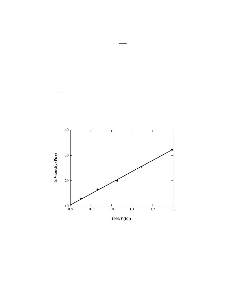
Excerpts from this work may be reproduced by instructors for distribution on a not-for-profit basis for testing or instructional purposes only to
students enrolled in courses for which the textbook has been adopted. Any other reproduction or translation of this work beyond that permitted
by Sections 107 or 108 of the 1976 United States Copyright Act without the permission of the copyright owner is unlawful.
13.13
The viscosity η of a glass varies with temperature according to the relationship
η = A exp
Q
vis
RT
where Q
vis
is the energy of activation for viscous flow, A is a temperature-independent constant, and R and T are,
respectively, the gas constant and the absolute temperature. A plot of ln η versus l/T should be nearly linear, and
with a slope of Q
vis
/R. Using the data in Figure 13.7, (a) make such a plot for the borosilicate glass, and (b)
determine the activation energy between temperatures of 500 and 900°C.
Solution
(a) Below is shown the logarithm viscosity versus reciprocal of temperature plot for the borosilicate glass,
using the data in Figure 13.7. The dashed line has been drawn through the data points corresponding to
temperatures between 500 and 900ºC (as stipulated in the problem statement).
(b) The activation energy, Q
vis
, may be computed according to

Excerpts from this work may be reproduced by instructors for distribution on a not-for-profit basis for testing or instructional purposes only to
students enrolled in courses for which the textbook has been adopted. Any other reproduction or translation of this work beyond that permitted
by Sections 107 or 108 of the 1976 United States Copyright Act without the permission of the copyright owner is unlawful.
Q
vis
= R
∆ ln η
∆
1
T
= R
ln
η
1
− ln η
2
1
T
1
−
1
T
2
where R is the gas constant, and
∆ ln η
∆
1
T
is the slope of the dashed line that has been constructed. Taking 1/T
1
and
1/T
2
as 0.8
× 10
-3
and 1.3
× 10
-3
K
-1
, respectively, then the corresponding values of ln
η
1
and ln
η
2
are 10.59 and
32.50. Therefore,
Q
vis
= R
ln
η
1
− ln η
2
1
T
1
−
1
T
2
= (8.31 J/mol − K)
10.59
− 32.50
0.8
× 10
−3
K
−1
− 1.3 × 10
−3
K
−1
= 364,000 J/mol

Excerpts from this work may be reproduced by instructors for distribution on a not-for-profit basis for testing or instructional purposes only to
students enrolled in courses for which the textbook has been adopted. Any other reproduction or translation of this work beyond that permitted
by Sections 107 or 108 of the 1976 United States Copyright Act without the permission of the copyright owner is unlawful.
13.14
For many viscous materials, the viscosity η may be defined in terms of the expression
η =
σ
d
ε/dt
where σ and dε/dt are, respectively, the tensile stress and the strain rate. A cylindrical specimen of a soda-lime
glass of diameter 5 mm (0.2 in.) and length 100 mm (4 in.) is subjected to a tensile force of 1 N (0.224 lb
f
) along its
axis. If its deformation is to be less than 1 mm (0.04 in.) over a week’s time, using Figure 13.7, determine the
maximum temperature to which the specimen may be heated.
Solution
This problem calls for us to determine the maximum temperature to which a cylindrical specimen of soda-
lime glass may be heated in order that its deformation be less than 1 mm over a week's time. According to Equation
6.1
σ =
F
A
0
=
1 N
π
5
× 10
−3
m
2
2
= 5.09
× 10
4
Pa
Also,
d
ε
dt
=
d
∆l
l
0
dt
=
1 mm /100 mm
(1 wk)(7 days / week)(24 h / day)(3600 s / h)
= 1.653
× 10
-8
s
-1
Thus,
η =
σ
d
ε/dt
=
5.09
× 10
4
Pa
1.653
× 10
−8
s
−1
= 3.1
× 10
12
Pa - s
From Figure 13.7, the temperature at which the viscosity of the soda-lime glass is 3.1
× 10
12
Pa-s is about 500
°C
(930
°F).

Excerpts from this work may be reproduced by instructors for distribution on a not-for-profit basis for testing or instructional purposes only to
students enrolled in courses for which the textbook has been adopted. Any other reproduction or translation of this work beyond that permitted
by Sections 107 or 108 of the 1976 United States Copyright Act without the permission of the copyright owner is unlawful.
13.15 (a) Explain why residual thermal stresses are introduced into a glass piece when it is cooled.
(b) Are thermal stresses introduced upon heating? Why or why not?
Solution
(a) Residual thermal stresses are introduced into a glass piece when it is cooled because surface and
interior regions cool at different rates, and, therefore, contract different amounts; since the material will experience
very little, if any deformation, stresses are established.
(b) Yes, thermal stresses will be introduced because of thermal expansion upon heating for the same
reason as for thermal contraction upon cooling.

Excerpts from this work may be reproduced by instructors for distribution on a not-for-profit basis for testing or instructional purposes only to
students enrolled in courses for which the textbook has been adopted. Any other reproduction or translation of this work beyond that permitted
by Sections 107 or 108 of the 1976 United States Copyright Act without the permission of the copyright owner is unlawful.
13.16 Borosilicate glasses and fused silica are resistant to thermal shock. Why is this so?
Solution
Borosilicate glasses and fused silica are resistant to thermal shock because they have relatively low
coefficients of thermal expansion; therefore, upon heating or cooling, the difference in the degree of expansion or
contraction across a cross-section of a ware that is constructed from these materials will be relatively low.

Excerpts from this work may be reproduced by instructors for distribution on a not-for-profit basis for testing or instructional purposes only to
students enrolled in courses for which the textbook has been adopted. Any other reproduction or translation of this work beyond that permitted
by Sections 107 or 108 of the 1976 United States Copyright Act without the permission of the copyright owner is unlawful.
13.17 In your own words, briefly describe what happens as a glass piece is thermally tempered.
Thermal tempering of glasses is described in Section 13.9.

Excerpts from this work may be reproduced by instructors for distribution on a not-for-profit basis for testing or instructional purposes only to
students enrolled in courses for which the textbook has been adopted. Any other reproduction or translation of this work beyond that permitted
by Sections 107 or 108 of the 1976 United States Copyright Act without the permission of the copyright owner is unlawful.
13.18 Glass pieces may also be strengthened by chemical tempering. With this procedure, the glass
surface is put in a state of compression by exchanging some of the cations near the surface with other cations
having a larger diameter. Suggest one type of cation that, by replacing Na
+
, will induce chemical tempering in a
soda–lime glass.
Solution
Chemical tempering will be accomplished by substitution, for Na
+
, another monovalent cation with a
slightly larger diameter. From Table 12.3, both K
+
and Cs
+
fill these criteria, having ionic radii of 0.138 and 0.170
nm, respectively, which are larger than the ionic radius of Na
+
(0.102 nm). In fact, soda-lime glasses are tempered
by a K
+
-Na
+
ion exchange.

Excerpts from this work may be reproduced by instructors for distribution on a not-for-profit basis for testing or instructional purposes only to
students enrolled in courses for which the textbook has been adopted. Any other reproduction or translation of this work beyond that permitted
by Sections 107 or 108 of the 1976 United States Copyright Act without the permission of the copyright owner is unlawful.
Fabrication and Processing of Clay Products
13.19 Cite the two desirable characteristics of clay minerals relative to fabrication processes.
Solution
Two desirable characteristics of clay minerals relative to fabrication processes are (1) they become
hydroplastic (and therefore formable) when mixed with water; and (2) during firing, clays melt over a range of
temperatures, which allows some fusion and bonding of the ware without complete melting and a loss of mechanical
integrity and shape.

Excerpts from this work may be reproduced by instructors for distribution on a not-for-profit basis for testing or instructional purposes only to
students enrolled in courses for which the textbook has been adopted. Any other reproduction or translation of this work beyond that permitted
by Sections 107 or 108 of the 1976 United States Copyright Act without the permission of the copyright owner is unlawful.
13.20 From a molecular perspective, briefly explain the mechanism by which clay minerals become
hydroplastic when water is added.
Solution
Clays become hydroplastic when water is added because the water molecules occupy regions between the
layered molecular sheets; these water molecules essentially eliminate the secondary molecular bonds between
adjacent sheets, and also form a thin film around the clay particles. The net result is that the clay particles are
relatively free to move past one another, which is manifested as the hydroplasticity phenomenon.

Excerpts from this work may be reproduced by instructors for distribution on a not-for-profit basis for testing or instructional purposes only to
students enrolled in courses for which the textbook has been adopted. Any other reproduction or translation of this work beyond that permitted
by Sections 107 or 108 of the 1976 United States Copyright Act without the permission of the copyright owner is unlawful.
13.21 (a) What are the three main components of a whiteware ceramic such as porcelain?
(b) What role does each component play in the forming and firing procedures?
Solution
(a) The three components of a whiteware ceramic are clay, quartz, and a flux.
(b) With regard to the role that each component plays:
Quartz acts as a filler material.
Clay facilitates the forming operation since, when mixed with water, the mass may be made to
become either hydroplastic or form a slip. Also, since clays melt over a range of temperatures, the shape of the piece
being fired will be maintained.
The flux facilitates the formation of a glass having a relatively low melting temperature.

Excerpts from this work may be reproduced by instructors for distribution on a not-for-profit basis for testing or instructional purposes only to
students enrolled in courses for which the textbook has been adopted. Any other reproduction or translation of this work beyond that permitted
by Sections 107 or 108 of the 1976 United States Copyright Act without the permission of the copyright owner is unlawful.
13.22 (a) Why is it so important to control the rate of drying of a ceramic body that has been
hydroplastically formed or slip cast?
(b) Cite three factors that influence the rate of drying, and explain how each affects the rate.
Solution
(a) It is important to control the rate of drying inasmuch as if the rate of drying is too rapid, there will be
nonuniform shrinkage between surface and interior regions, such that warping and/or cracking of the ceramic ware
may result.
(b) Three factors that affect the rate of drying are temperature, humidity, and rate of air flow. The rate of
drying is enhanced by increasing both the temperature and rate of air flow, and by decreasing the humidity of the
air.

Excerpts from this work may be reproduced by instructors for distribution on a not-for-profit basis for testing or instructional purposes only to
students enrolled in courses for which the textbook has been adopted. Any other reproduction or translation of this work beyond that permitted
by Sections 107 or 108 of the 1976 United States Copyright Act without the permission of the copyright owner is unlawful.
13.23 Cite one reason why drying shrinkage is greater for slip cast or hydroplastic products that have
smaller clay particles.
Solution
The reason that drying shrinkage is greater for products having smaller clay particles is because there is
more particle surface area, and, consequently, more water will surround a given volume of particles. The drying
shrinkage will thus be greater as this water is removed, and as the interparticle separation decreases.

Excerpts from this work may be reproduced by instructors for distribution on a not-for-profit basis for testing or instructional purposes only to
students enrolled in courses for which the textbook has been adopted. Any other reproduction or translation of this work beyond that permitted
by Sections 107 or 108 of the 1976 United States Copyright Act without the permission of the copyright owner is unlawful.
13.24 (a) Name three factors that influence the degree to which vitrification occurs in clay-based ceramic
wares.
(b) Explain how density, firing distortion, strength, corrosion resistance, and thermal conductivity are
affected by the extent of vitrification.
Solution
(a) Three factors that influence the degree to which vitrification occurs in clay-based ceramic wares are:
(1) composition (especially the concentration of flux present); (2) the temperature of firing; and (3) the time at the
firing temperature.
(b) Density will increase with degree of vitrification since the total remaining pore volume decreases.
Firing distortion will increase with degree of vitrification since more liquid phase will be present at the
firing temperature.
Strength will also increase with degree of vitrification inasmuch as more of the liquid phase forms, which
fills in a greater fraction of pore volume. Upon cooling, the liquid forms a glass matrix of relatively high strength.
Corrosion resistance normally increases also, especially at service temperatures below that at which the
glass phase begins to soften. The rate of corrosion is dependent on the amount of surface area exposed to the
corrosive medium; hence, decreasing the total surface area by filling in some of the surface pores, diminishes the
corrosion rate.
Thermal conductivity will increase with degree of vitrification. The glass phase has a higher conductivity
than the pores that it has filled.

Excerpts from this work may be reproduced by instructors for distribution on a not-for-profit basis for testing or instructional purposes only to
students enrolled in courses for which the textbook has been adopted. Any other reproduction or translation of this work beyond that permitted
by Sections 107 or 108 of the 1976 United States Copyright Act without the permission of the copyright owner is unlawful.
Powder Pressing
13.25 Some ceramic materials are fabricated by hot isostatic pressing. Cite some of the limitations and
difficulties associated with this technique.
Solution
The principal disadvantage of hot-isostatic pressing is that it is expensive. The pressure is applied on a
pre-formed green piece by a gas. Thus, the process is slow, and the equipment required to supply the gas and
withstand the elevated temperature and pressure is costly.

Excerpts from this work may be reproduced by instructors for distribution on a not-for-profit basis for testing or instructional purposes only to
students enrolled in courses for which the textbook has been adopted. Any other reproduction or translation of this work beyond that permitted
by Sections 107 or 108 of the 1976 United States Copyright Act without the permission of the copyright owner is unlawful.
DESIGN PROBLEM
13.D1 Some of our modern kitchen cookware is made of ceramic materials.
(a) List at least three important characteristics required of a material to be used for this application.
(b) Make a comparison of three ceramic materials as to their relative properties and, in addition, to cost.
(c) On the basis of this comparison, select the material most suitable for the cookware.
Solution
(a) Important characteristics that are required of a ceramic material to be used for kitchen cookware are:
(1) it must have a high resistance to thermal shock (Section 19.5) in order to withstand relatively rapid changes in
temperature; (2) it must have a relatively high thermal conductivity; 3) it must be relatively strong and tough in
order to endure normal kitchen use; and 4) it must be nontoxic.
(b) Possible materials worth considering are a common soda-lime glass, a borosilicate (Pyrex) glass, and a
glass ceramic. These materials and some of their characteristics are discussed in this chapter. Using Equation 17.9
a comparison of the resistance to thermal shock may be made. The student will need to obtain cost information.
(c) It is left to the student to make this determination and justify the decision.
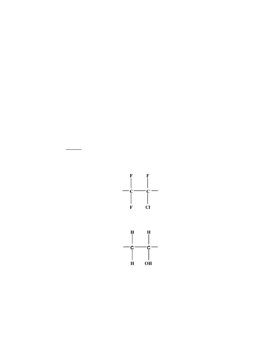
Excerpts from this work may be reproduced by instructors for distribution on a not-for-profit basis for testing or instructional purposes only to
students enrolled in courses for which the textbook has been adopted. Any other reproduction or translation of this work beyond that permitted
by Sections 107 or 108 of the 1976 United States Copyright Act without the permission of the copyright owner is unlawful.
CHAPTER 14
POLYMER STRUCTURES
PROBLEM SOLUTIONS
Hydrocarbon Molecules
Polymer Molecules
The Chemistry of Polymer Molecules
14.1 On the basis of the structures presented in this chapter, sketch repeat unit structures for the following
polymers: (a) polychlorotrifluoroethylene, and (b) poly(vinyl alcohol).
Solution
The repeat unit structures called for are sketched below.
(a) Polychlorotrifluoroethylene
(b) Poly(vinyl alcohol)

Excerpts from this work may be reproduced by instructors for distribution on a not-for-profit basis for testing or instructional purposes only to
students enrolled in courses for which the textbook has been adopted. Any other reproduction or translation of this work beyond that permitted
by Sections 107 or 108 of the 1976 United States Copyright Act without the permission of the copyright owner is unlawful.
Molecular Weight
14.2 Compute repeat unit molecular weights for the following: (a) poly(vinyl chloride), (b) poly(ethylene
terephthalate), (c) polycarbonate, and (d) polydimethylsiloxane.
Solution
(a) For poly(vinyl chloride), each repeat unit consists of two carbons, three hydrogens, and one chlorine
(Table 14.3). If A
C
, A
H
and A
Cl
represent the atomic weights of carbon, hydrogen, and chlorine, respectively, then
m = 2(A
C
) + 3(A
H
) + (A
Cl
)
= (2)(12.01 g/mol) + (3)(1.008 g/mol) + 35.45 g/mol = 62.49 g/mol
(b) For poly(ethylene terephthalate), from Table 14.3, each repeat unit has ten carbons, eight hydrogens,
and four oxygens. Thus,
m = 10(A
C
) + 8(A
H
) + 4(A
O
)
= (10)(12.01 g/mol) + (8)(1.008 g/mol) + (4)(16.00 g/mol) = 192.16 g/mol
(c) For polycarbonate, from Table 14.3, each repeat unit has sixteen carbons, fourteen hydrogens, and
three oxygens. Thus,
m = 16(A
C
) + 14(A
H
) + 3(A
O
)
= (16)(12.01 g/mol) + (14)(1.008 g/mol) + (3)(16.00 g/mol)
= 254.27 g/mol
(d) For polydimethylsiloxane, from Table 14.5, each repeat unit has two carbons, six hydrogens, one
silicon and one oxygen. Thus,
m = 2(A
C
) + 6(A
H
) + (A
Si
) + (A
O
)
= (2)(12.01 g/mol) + (6)(1.008 g/mol) + (28.09 g/mol) + (16.00 g/mol) = 74.16 g/mol

Excerpts from this work may be reproduced by instructors for distribution on a not-for-profit basis for testing or instructional purposes only to
students enrolled in courses for which the textbook has been adopted. Any other reproduction or translation of this work beyond that permitted
by Sections 107 or 108 of the 1976 United States Copyright Act without the permission of the copyright owner is unlawful.
14.3 The number-average molecular weight of a polypropylene is 1,000,000 g/mol. Compute the degree of
polymerization.
Solution
We are asked to compute the degree of polymerization for polypropylene, given that the number-average
molecular weight is 1,000,000 g/mol. The repeat unit molecular weight of polypropylene is just
m = 3(A
C
) + 6(A
H
)
= (3)(12.01 g/mol) + (6)(1.008 g/mol) = 42.08 g/mol
Now it is possible to compute the degree of polymerization using Equation 14.6 as
DP =
M
n
m
=
1, 000, 000 g/mol
42.08 g/mol
= 23, 760

Excerpts from this work may be reproduced by instructors for distribution on a not-for-profit basis for testing or instructional purposes only to
students enrolled in courses for which the textbook has been adopted. Any other reproduction or translation of this work beyond that permitted
by Sections 107 or 108 of the 1976 United States Copyright Act without the permission of the copyright owner is unlawful.
14.4 (a) Compute the repeat unit molecular weight of polystyrene.
(b) Compute the number-average molecular weight for a polystyrene for which the degree of
polymerization is 25,000.
Solution
(a) The repeat unit molecular weight of polystyrene is called for in this portion of the problem. For
polystyrene, from Table 14.3, each repeat unit has eight carbons and eight hydrogens. Thus,
m = 8(A
C
) + 8(A
H
)
= (8)(12.01 g/mol) + (8)(1.008 g/mol) = 104.14 g/mol
(b) We are now asked to compute the number-average molecular weight. Since the degree of
polymerization is 25,000, using Equation 14.6
M
n
= (DP)m = (25, 000)(104.14 g/mol) = 2.60
× 10
6
g/mol

Excerpts from this work may be reproduced by instructors for distribution on a not-for-profit basis for testing or instructional purposes only to
students enrolled in courses for which the textbook has been adopted. Any other reproduction or translation of this work beyond that permitted
by Sections 107 or 108 of the 1976 United States Copyright Act without the permission of the copyright owner is unlawful.
14.5 Below, molecular weight data for a polypropylene material are tabulated. Compute (a) the number-
average molecular weight, (b) the weight-average molecular weight, and (c) the degree of polymerization.
Molecular Weight
Range (g/mol)
x
i
w
i
8,000–16,000
0.05
0.02
16,000–24,000
0.16
0.10
24,000–32,000
0.24
0.20
32,000–40,000
0.28
0.30
40,000–48,000
0.20
0.27
48,000–56,000
0.07
0.11
Solution
(a) From the tabulated data, we are asked to compute
M
n
, the number-average molecular weight. This is
carried out below.
Molecular wt
Range
Mean Mi
xi
xiMi
8,000-16,000
12,000
0.05
600
16,000-24,000
20,000
0.16
3200
24,000-32,000
28,000
0.24
6720
32,000-40,000
36,000
0.28
10,080
40,000-48,000
44,000
0.20
8800
48,000-56,000
52,000
0.07
3640
____________________________
M
n
=
x
i
M
i
∑
= 33, 040 g/mol
(b) From the tabulated data, we are asked to compute
M
w
, the weight-average molecular weight.
Molecular wt.
Range
Mean M
i
w
i
w
i
M
i
8,000-16,000
12,000
0.02
240
16,000-24,000
20,000
0.10
2000
24,000-32,000
28,000
0.20
5600

Excerpts from this work may be reproduced by instructors for distribution on a not-for-profit basis for testing or instructional purposes only to
students enrolled in courses for which the textbook has been adopted. Any other reproduction or translation of this work beyond that permitted
by Sections 107 or 108 of the 1976 United States Copyright Act without the permission of the copyright owner is unlawful.
32,000-40,000
36,000
0.30
10,800
40,000-48,000
44,000
0.27
11,880
48,000-56,000
52,000
0.11
5720
___________________________
M
w
=
w
i
M
i
∑
= 36, 240 g/mol
(c) Now we are asked to compute the degree of polymerization, which is possible using Equation 14.6.
For polypropylene, the repeat unit molecular weight is just
m = 3(A
C
) + 6(A
H
)
= (3)(12.01 g/mol) + (6)(1.008 g/mol) = 42.08 g/mol
And
DP =
M
n
m
=
33, 040 g/mol
42.08 g/mol
= 785

Excerpts from this work may be reproduced by instructors for distribution on a not-for-profit basis for testing or instructional purposes only to
students enrolled in courses for which the textbook has been adopted. Any other reproduction or translation of this work beyond that permitted
by Sections 107 or 108 of the 1976 United States Copyright Act without the permission of the copyright owner is unlawful.
14.6 Molecular weight data for some polymer are tabulated here. Compute (a) the number-average
molecular weight, and (b) the weight-average molecular weight. (c) If it is known that this material's degree of
polymerization is 710, which one of the polymers listed in Table 14.3 is this polymer? Why?
Molecular Weight
Range g/mol
x
i
w
i
15,000–30,000
0.04
0.01
30,000–45,000
0.07
0.04
45,000–60,000
0.16
0.11
60,000–75,000
0.26
0.24
75,000–90,000
0.24
0.27
90,000–105,000
0.12
0.16
105,000–120,000
0.08
0.12
120,000–135,000
0.03
0.05
Solution
(a) From the tabulated data, we are asked to compute
M
n
, the number-average molecular weight. This is
carried out below.
Molecular wt.
Range
Mean M
i
x
i
x
i
M
i
15,000-30,000
22,500
0.04
900
30,000-45,000
37,500
0.07
2625
45,000-60,000
52,500
0.16
8400
60,000-75,000
67,500
0.26
17,550
75,000-90,000
82,500
0.24
19,800
90,000-105,000
97,500
0.12
11,700
105,000-120,000
112,500
0.08
9000
120,000-135,000
127,500
0.03
3825
_________________________
M
n
=
x
i
M
i
∑
= 73,800 g/mol

Excerpts from this work may be reproduced by instructors for distribution on a not-for-profit basis for testing or instructional purposes only to
students enrolled in courses for which the textbook has been adopted. Any other reproduction or translation of this work beyond that permitted
by Sections 107 or 108 of the 1976 United States Copyright Act without the permission of the copyright owner is unlawful.
(b) From the tabulated data, we are asked to compute
M
w
, the weight-average molecular weight. This
determination is performed as follows:
Molecular wt.
Range
Mean M
i
w
i
w
i
M
i
15,000-30,000
22,500
0.01
225
30,000-45,000
37,500
0.04
1500
45,000-60,000
52,500
0.11
5775
60,000-75,000
67,500
0.24
16,200
75,000-90,000
82,500
0.27
22,275
90,000-105,000
97,500
0.16
15,600
105,000-120,000
112,500
0.12
13,500
120,000-135,000
127,500
0.05
6375
_________________________
M
w
=
w
i
M
i
∑
= 81, 450 g/mol
(c) We are now asked if the degree of polymerization is 710, which of the polymers in Table 14.3 is this
material? It is necessary to compute m in Equation 14.6 as
m =
M
n
DP
=
73,800 g/mol
710
= 103.94 g/mol
The repeat unit molecular weights of the polymers listed in Table 14.3 are as follows:
Polyethylene--28.05 g/mol
Poly(vinyl chloride)--62.49 g/mol
Polytetrafluoroethylene--100.02 g/mol
Polypropylene--42.08 g/mol
Polystyrene--104.14 g/mol
Poly(methyl methacrylate)--100.11 g/mol
Phenol-formaldehyde--133.16 g/mol
Nylon 6,6--226.32 g/mol
PET--192.16 g/mol
Polycarbonate--254.27 g/mol
Therefore, polystyrene is the material since its repeat unit molecular weight is closest to that calculated above.

Excerpts from this work may be reproduced by instructors for distribution on a not-for-profit basis for testing or instructional purposes only to
students enrolled in courses for which the textbook has been adopted. Any other reproduction or translation of this work beyond that permitted
by Sections 107 or 108 of the 1976 United States Copyright Act without the permission of the copyright owner is unlawful.
14.7 Is it possible to have a poly(methyl methacrylate) homopolymer with the following molecular weight
data and a of polymerization of 527? Why or why not?
Molecular Weight
Range (g/mol)
w
i
x
i
8,000–20,000
0.02
0.05
20,000–32,000
0.08
0.15
32,000–44,000
0.17
0.21
44,000–56,000
0.29
0.28
56,000–68,000
0.23
0.18
68,000–80,000
0.16
0.10
80,000–92,000
0.05
0.03
Solution
This problem asks if it is possible to have a poly(methyl methacrylate) homopolymer with the given
molecular weight data and a degree of polymerization of 527. The appropriate data are given below along with a
computation of the number-average molecular weight.
Molecular wt.
Range
Mean M
i
x
i
x
i
M
i
8,000-20,000
14,000
0.05
700
20,000-32,000
26,000
0.15
3900
32,000-44,000
38,000
0.21
7980
44,000-56,000
50,000
0.28
14,000
56,000-68,000
62,000
0.18
11,160
68,000-80,000
74,000
0.10
7400
80,000-92,000
86,000
0.03
2580
_________________________
M
n
=
x
i
M
i
∑
= 47, 720 g/mol
For PMMA, from Table 14.3, each repeat unit has five carbons, eight hydrogens, and two oxygens. Thus,
m = 5(A
C
) + 8(A
H
) + 2(A
O
)

Excerpts from this work may be reproduced by instructors for distribution on a not-for-profit basis for testing or instructional purposes only to
students enrolled in courses for which the textbook has been adopted. Any other reproduction or translation of this work beyond that permitted
by Sections 107 or 108 of the 1976 United States Copyright Act without the permission of the copyright owner is unlawful.
= (5)(12.01 g/mol) + (8)(1.008 g/mol) + (2)(16.00 g/mol) = 100.11 g/mol
Now, we will compute the degree of polymerization using Equation 14.6 as
DP =
M
n
m
=
47, 720 g/mol
100.11 g/mol
= 477
Thus, such a homopolymer is not possible since the calculated degree of polymerization is 477 (and not 527).

Excerpts from this work may be reproduced by instructors for distribution on a not-for-profit basis for testing or instructional purposes only to
students enrolled in courses for which the textbook has been adopted. Any other reproduction or translation of this work beyond that permitted
by Sections 107 or 108 of the 1976 United States Copyright Act without the permission of the copyright owner is unlawful.
14.8 High-density polyethylene may be chlorinated by inducing the random substitution of chlorine atoms
for hydrogen.
(a) Determine the concentration of Cl (in wt%) that must be added if this substitution occurs for 5% of all
the original hydrogen atoms.
(b) In what ways does this chlorinated polyethylene differ from poly(vinyl chloride)?
Solution
(a) For chlorinated polyethylene, we are asked to determine the weight percent of chlorine added for 5%
Cl substitution of all original hydrogen atoms. Consider 50 carbon atoms; there are 100 possible side-bonding
sites. Ninety-five are occupied by hydrogen and five are occupied by Cl. Thus, the mass of these 50 carbon atoms,
m
C
, is just
m
C
= 50(A
C
) = (50)(12.01 g/mol) = 600.5 g
Likewise, for hydrogen and chlorine,
m
H
= 95(A
H
) = (95)(1.008 g/mol) = 95.76 g
m
Cl
= 5(A
Cl
) = (5)(35.45 g/mol) = 177.25 g
Thus, the concentration of chlorine, C
Cl
, is determined using a modified form of Equation 4.3 as
C
Cl
=
m
Cl
m
C
+ m
H
+ m
Cl
x 100
=
177.25 g
600.5 g + 95.76 g + 177.25 g
× 100 = 20.3 wt%
(b) Chlorinated polyethylene differs from poly(vinyl chloride), in that, for PVC, (1) 25% of the side-
bonding sites are substituted with Cl, and (2) the substitution is probably much less random.

Excerpts from this work may be reproduced by instructors for distribution on a not-for-profit basis for testing or instructional purposes only to
students enrolled in courses for which the textbook has been adopted. Any other reproduction or translation of this work beyond that permitted
by Sections 107 or 108 of the 1976 United States Copyright Act without the permission of the copyright owner is unlawful.
Molecular Shape
14.9 For a linear polymer molecule, the total chain length L depends on the bond length between chain
atoms d, the total number of bonds in the molecule N, and the angle between adjacent backbone chain atoms
θ, as
follows:
L = Nd sin
θ
2
(14.11)
Furthermore, the average end-to-end distance for a series of polymer molecules r in Figure 14.6 is equal to
r = d
N
(14.12)
A linear polytetrafluoroethylene has a number-average molecular weight of 500,000 g/mol; compute average
values of L and r for this material.
Solution
This problem first of all asks for us to calculate, using Equation 14.11, the average total chain length, L, for
a linear polytetrafluoroethylene polymer having a number-average molecular weight of 500,000 g/mol. It is
necessary to calculate the degree of polymerization, DP, using Equation 14.6. For polytetrafluoroethylene, from
Table 14.3, each repeat unit has two carbons and four flourines. Thus,
m = 2(A
C
) + 4(A
F
)
= (2)(12.01 g/mol) + (4)(19.00 g/mol) = 100.02 g/mol
and
DP =
M
n
m
=
500, 000 g/mol
100.02 g/mol
= 5000
which is the number of repeat units along an average chain. Since there are two carbon atoms per repeat unit, there
are two C—C chain bonds per repeat unit, which means that the total number of chain bonds in the molecule, N, is
just (2)(5000) = 10,000 bonds. Furthermore, assume that for single carbon-carbon bonds, d = 0.154 nm and
θ =
109
° (Section 14.4); therefore, from Equation 14.11
L = Nd sin
θ
2

Excerpts from this work may be reproduced by instructors for distribution on a not-for-profit basis for testing or instructional purposes only to
students enrolled in courses for which the textbook has been adopted. Any other reproduction or translation of this work beyond that permitted
by Sections 107 or 108 of the 1976 United States Copyright Act without the permission of the copyright owner is unlawful.
= (10,000)(0.154 nm) sin
109
°
2
= 1254 nm
It is now possible to calculate the average chain end-to-end distance, r, using Equation 14.12 as
r = d
N = (0.154 nm) 10, 000 = 15.4 nm

Excerpts from this work may be reproduced by instructors for distribution on a not-for-profit basis for testing or instructional purposes only to
students enrolled in courses for which the textbook has been adopted. Any other reproduction or translation of this work beyond that permitted
by Sections 107 or 108 of the 1976 United States Copyright Act without the permission of the copyright owner is unlawful.
14.10 Using the definitions for total chain molecule length, L (Equation 14.11) and average chain end-to-
end distance r (Equation 14.12), for a linear polyethylene determine:
(a) the number-average molecular weight for L = 2500 nm;
(b) the number-average molecular weight for r = 20 nm.
Solution
(a) This portion of the problem asks for us to calculate the number-average molecular weight for a linear
polyethylene for which L in Equation 14.11 is 2500 nm. It is first necessary to compute the value of N using this
equation, where, for the C—C chain bond, d = 0.154 nm, and
θ = 109°. Thus
N =
L
d sin
θ
2
=
2500 nm
(0.154 nm) sin
109
°
2
= 19, 940
Since there are two C—C bonds per polyethylene repeat unit, there is an average of N/2 or 19,940/2 = 9970 repeat
units per chain, which is also the degree of polymerization, DP. In order to compute the value of
M
n
using
Equation 14.6, we must first determine m for polyethylene. Each polyethylene repeat unit consists of two carbon
and four hydrogen atoms, thus
m = 2(A
C
) + 4(A
H
)
= (2)(12.01 g/mol) + (4)(1.008 g/mol) = 28.05 g/mol
Therefore
M
n
= (DP)m = (9970)(28.05 g/mol) = 280, 000 g/mol
(b) Next, we are to determine the number-average molecular weight for r = 20 nm. Solving for N from
Equation 14.12 leads to
N =
r
2
d
2
=
(20 nm)
2
(0.154 nm)
2
= 16, 900

Excerpts from this work may be reproduced by instructors for distribution on a not-for-profit basis for testing or instructional purposes only to
students enrolled in courses for which the textbook has been adopted. Any other reproduction or translation of this work beyond that permitted
by Sections 107 or 108 of the 1976 United States Copyright Act without the permission of the copyright owner is unlawful.
which is the total number of bonds per average molecule. Since there are two C—C bonds per repeat unit, then DP
= N/2 = 16,900/2 = 8450. Now, from Equation 14.6
M
n
= (DP)m = (8450)(28.05 g/mol) = 237, 000 g/mol
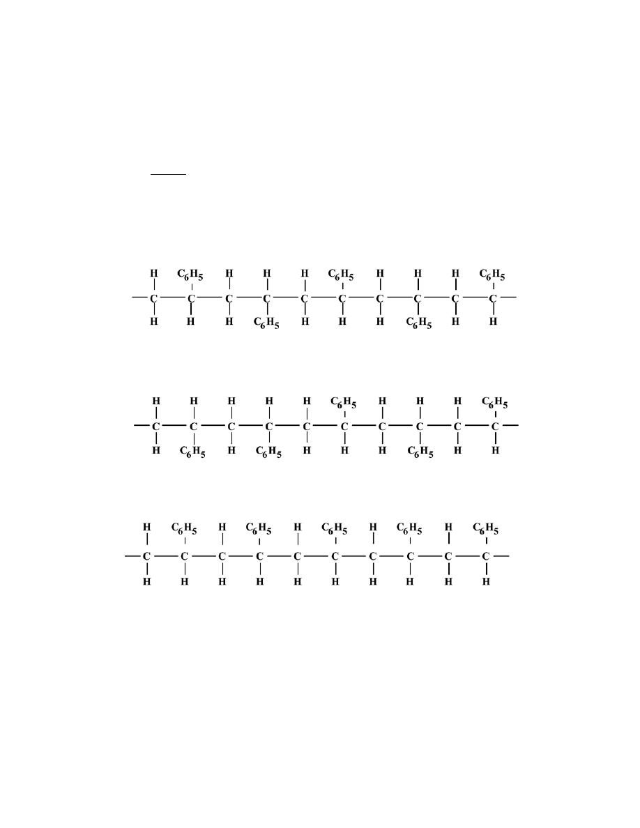
Excerpts from this work may be reproduced by instructors for distribution on a not-for-profit basis for testing or instructional purposes only to
students enrolled in courses for which the textbook has been adopted. Any other reproduction or translation of this work beyond that permitted
by Sections 107 or 108 of the 1976 United States Copyright Act without the permission of the copyright owner is unlawful.
Molecular Configurations
14.11 Sketch portions of a linear polystyrene molecule that are (a) syndiotactic, (b) atactic, and (c)
isotactic. Use two-dimensional schematics per footnote 8 of this chapter.
Solution
We are asked to sketch portions of a linear polystyrene molecule for different configurations (using two-
dimensional schematic sketches).
(a) Syndiotactic polystyrene
(b) Atactic polystyrene
(c) Isotactic polystyrene
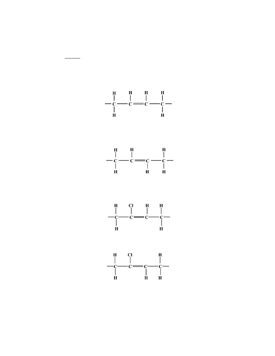
Excerpts from this work may be reproduced by instructors for distribution on a not-for-profit basis for testing or instructional purposes only to
students enrolled in courses for which the textbook has been adopted. Any other reproduction or translation of this work beyond that permitted
by Sections 107 or 108 of the 1976 United States Copyright Act without the permission of the copyright owner is unlawful.
14.12 Sketch cis and trans structures for (a) butadiene, and (b) chloroprene. Use two-dimensional
schematics per footnote 11 of this chapter.
Solution
This problem asks for us to sketch cis and trans structures for butadiene and chloroprene.
(a) The structure for cis polybutadiene (Table 14.5) is
The structure of trans butadiene is
(b) The structure of cis chloroprene (Table 14.5) is
The structure of trans chloroprene is

Excerpts from this work may be reproduced by instructors for distribution on a not-for-profit basis for testing or instructional purposes only to
students enrolled in courses for which the textbook has been adopted. Any other reproduction or translation of this work beyond that permitted
by Sections 107 or 108 of the 1976 United States Copyright Act without the permission of the copyright owner is unlawful.
Thermoplastic and Thermosetting Polymers
14.13 Make comparisons of thermoplastic and thermosetting polymers (a) on the basis of mechanical
characteristics upon heating, and (b) according to possible molecular structures.
Solution
(a) Thermoplastic polymers soften when heated and harden when cooled, whereas thermosetting polymers,
harden upon heating, while further heating will not lead to softening.
(b) Thermoplastic polymers have linear and branched structures, while for thermosetting polymers, the
structures will normally be network or crosslinked.

Excerpts from this work may be reproduced by instructors for distribution on a not-for-profit basis for testing or instructional purposes only to
students enrolled in courses for which the textbook has been adopted. Any other reproduction or translation of this work beyond that permitted
by Sections 107 or 108 of the 1976 United States Copyright Act without the permission of the copyright owner is unlawful.
14.14 (a) Is it possible to grind up and reuse phenol-formaldehyde? Why or why not?
(b) Is it possible to grind up and reuse polypropylene? Why or why not?
Solution
(a) It is not possible to grind up and reuse phenol-formaldehyde because it is a network thermoset polymer
and, therefore, is not amenable to remolding.
(b) Yes, it is possible to grind up and reuse polypropylene since it is a thermoplastic polymer, will soften
when reheated, and, thus, may be remolded.
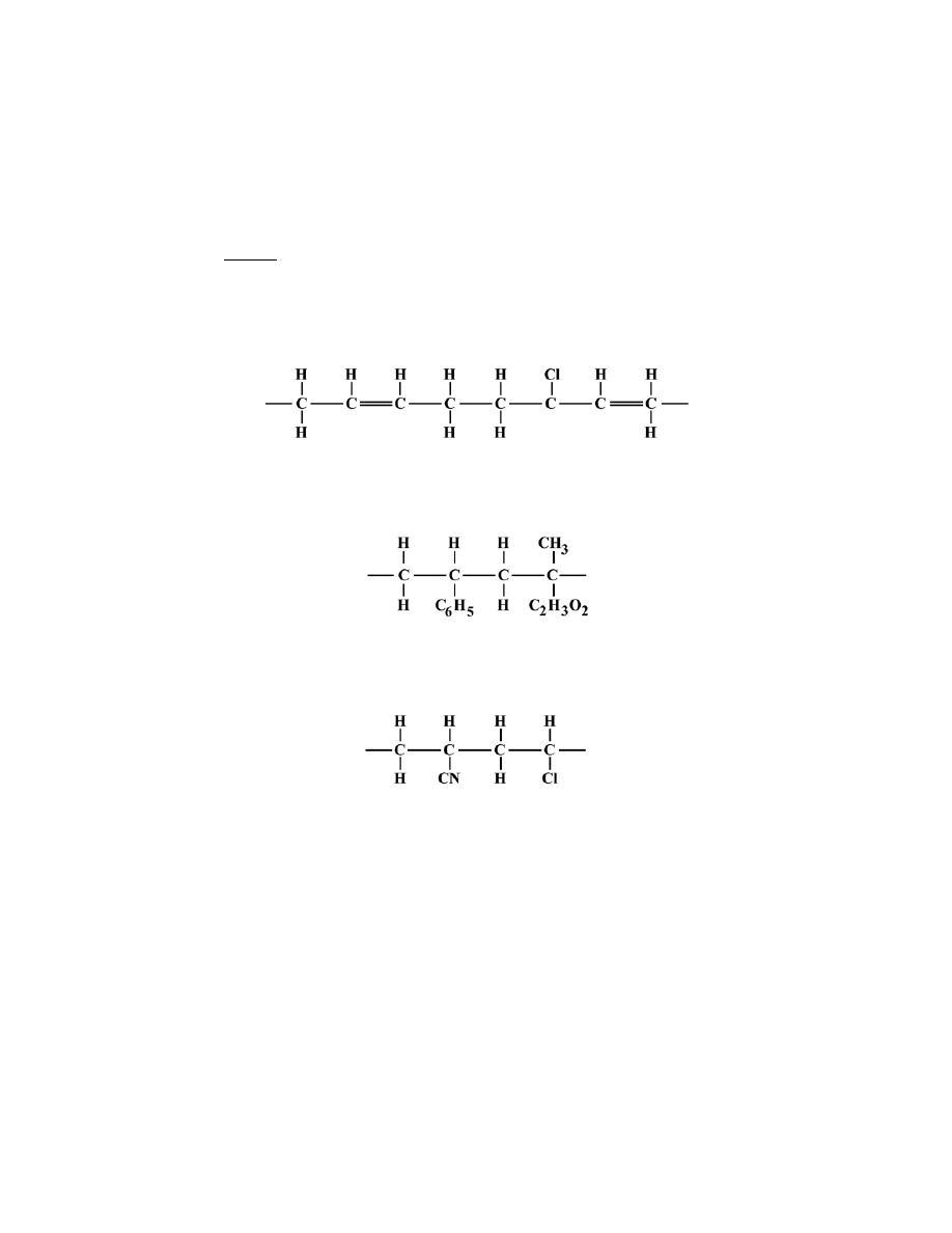
Excerpts from this work may be reproduced by instructors for distribution on a not-for-profit basis for testing or instructional purposes only to
students enrolled in courses for which the textbook has been adopted. Any other reproduction or translation of this work beyond that permitted
by Sections 107 or 108 of the 1976 United States Copyright Act without the permission of the copyright owner is unlawful.
Copolymers
14.15 Sketch the repeat structure for each of the following alternating copolymers: (a) poly(butadiene-
chloroprene), (b) poly(styrene-methyl methacrylate), and (c) poly(acrylonitrile-vinyl chloride).
Solution
This problem asks for sketches of the repeat unit structures for several alternating copolymers.
(a) For poly(butadiene-chloroprene)
(b) For poly(styrene-methyl methacrylate)
(c) For poly(acrylonitrile-vinyl chloride)

Excerpts from this work may be reproduced by instructors for distribution on a not-for-profit basis for testing or instructional purposes only to
students enrolled in courses for which the textbook has been adopted. Any other reproduction or translation of this work beyond that permitted
by Sections 107 or 108 of the 1976 United States Copyright Act without the permission of the copyright owner is unlawful.
14.16 The number-average molecular weight of a poly(styrene-butadiene) alternating copolymer is
1,350,000 g/mol; determine the average number of styrene and butadiene repeat units per molecule.
Solution
Since it is an alternating copolymer, the number of both types of repeat units will be the same. Therefore,
consider them as a single repeat unit, and determine the number-average degree of polymerization. For the styrene
repeat unit, there are eight carbon atoms and eight hydrogen atoms, while the butadiene repeat consists of four
carbon atoms and six hydrogen atoms. Therefore, the styrene-butadiene combined repeat unit weight is just
m = 12(A
C
) + 14(A
H
)
= (12)(12.01 g/mol) + (14)(1.008 g/mol) = 158.23 g/mol
From Equation 14.6, the degree of polymerization is just
DP =
M
n
m
=
1, 350, 000 g/mol
158.23 g/mol
= 8530
Thus, there is an average of 8530 of both repeat unit types per molecule.

Excerpts from this work may be reproduced by instructors for distribution on a not-for-profit basis for testing or instructional purposes only to
students enrolled in courses for which the textbook has been adopted. Any other reproduction or translation of this work beyond that permitted
by Sections 107 or 108 of the 1976 United States Copyright Act without the permission of the copyright owner is unlawful.
14.17 Calculate the number-average molecular weight of a random nitrile rubber [poly(acrylonitrile-
butadiene) copolymer] in which the fraction of butadiene repeat units is 0.30; assume that this concentration
corresponds to a degree of polymerization of 2000.
Solution
This problem asks for us to calculate the number-average molecular weight of a random nitrile rubber
copolymer. For the acrylonitrile repeat unit there are three carbon, one nitrogen, and three hydrogen atoms. Thus,
its repeat unit molecular weight is
m
Ac
= 3(A
C
) + (A
N
) + 3(A
H
)
= (3)(12.01 g/mol) + 14.01 g/mol + (3)(1.008 g/mol) = 53.06 g/mol
The butadiene repeat unit is composed of four carbon and six hydrogen atoms. Thus, its repeat unit molecular
weight is
m
Bu
= 4(A
C
) + 6(A
H
)
= (4)(12.01 g/mol) + (6)(1.008 g/mol) = 54.09 g/mol
From Equation 14.7, the average repeat unit molecular weight is just
m = f
Ac
m
Ac
+ f
Bu
m
Bu
= (0.70)(53.06 g/mol) + (0.30)(54.09 g/mol) = 53.37 g/mol
Since DP = 2000 (as stated in the problem),
M
n
may be computed using Equation 14.6 as
M
n
= m (DP) = (53.37 g/mol)(2000) = 106, 740 g/mol

Excerpts from this work may be reproduced by instructors for distribution on a not-for-profit basis for testing or instructional purposes only to
students enrolled in courses for which the textbook has been adopted. Any other reproduction or translation of this work beyond that permitted
by Sections 107 or 108 of the 1976 United States Copyright Act without the permission of the copyright owner is unlawful.
14.18 An alternating copolymer is known to have a number-average molecular weight of 250,000 g/mol
and a degree of polymerization of 3420. If one of the repeat units is styrene, which of ethylene, propylene,
tetrafluoroethylene, and vinyl chloride is the other repeat unit? Why?
Solution
For an alternating copolymer which has a number-average molecular weight of 250,000 g/mol and a degree
of polymerization of 3420, we are to determine one of the repeat unit types if the other is styrene. It is first
necessary to calculate
m using Equation 14.6 as
m =
M
n
DP
=
250, 000 g/mol
3420
= 73.10 g/mol
Since this is an alternating copolymer we know that chain fraction of each repeat unit type is 0.5; that is f
s
= f
x
=
0.5, f
s
and f
x
being, respectively, the chain fractions of the styrene and unknown repeat units. Also, the repeat unit
molecular weight for styrene is
m
s
= 8(A
C
) + 8(A
H
)
= 8(12.01 g/mol) + 8(1.008 g/mol) = 104.14 g/mol
Now, using Equation 14.7, it is possible to calculate the repeat unit weight of the unknown repeat unit type, m
x
.
Thus
m
x
=
m
− f
s
m
s
f
x
=
73.10 g/mol - (0.5)(104.14 g/mol)
0.5
= 42.06 g/mol
Finally, it is necessary to calculate the repeat unit molecular weights for each of the possible other repeat
unit types. These are calculated below:
m
ethylene
= 2(A
C
) + 4(A
H
) = 2(12.01 g/mol) + 4(1.008 g/mol) = 28.05 g/mol
m
propylene
= 3(A
C
) + 6(A
H
) = 3(12.01 g/mol) + 6(1.008 g/mol) = 42.08 g/mol
m
TFE
= 2(A
C
) + 4(A
F
) = 2(12.01 g/mol) + 4(19.00 g/mol) = 100.02 g/mol
m
VC
= 2(A
C
) + 3(A
H
) + (A
Cl
) = 2(12.01 g/mol) + 3(1.008 g/mol) + 35.45 g/mol = 62.49 g/mol
Therefore, propylene is the other repeat unit type since its m value is almost the same as the calculated m
x
.

Excerpts from this work may be reproduced by instructors for distribution on a not-for-profit basis for testing or instructional purposes only to
students enrolled in courses for which the textbook has been adopted. Any other reproduction or translation of this work beyond that permitted
by Sections 107 or 108 of the 1976 United States Copyright Act without the permission of the copyright owner is unlawful.
14.19 (a) Determine the ratio of butadiene to styrene repeat units in a copolymer having a number-
average molecular weight of 350,000 g/mol and degree of polymerization of 4425.
(b) Which type(s) of copolymer(s) will this copolymer be, considering the following possibilities: random,
alternating, graft, and block? Why?
Solution
(a) This portion of the problem asks us to determine the ratio of butadiene to styrene repeat units in a
copolymer having a weight-average molecular weight of 350,000 g/mol and a degree of polymerization of 4425. It
first becomes necessary to calculate the average repeat unit molecular weight of the copolymer,
m , using Equation
14.6 as
m =
M
n
DP
=
350, 000 g/mol
4425
= 79.10 g/mol
If we designate f
b
as the chain fraction of butadiene repeat units, since the copolymer consists of only two repeat
unit types, the chain fraction of styrene repeat units f
s
is just 1 – f
b
. Now, Equation 14.7 for this copolymer may be
written in the form
m = f
b
m
b
+ f
s
m
s
= f
b
m
b
+ (1
− f
b
)m
s
in which m
b
and m
s
are the repeat unit molecular weights for butadiene and styrene, respectively. These values are
calculated as follows:
m
b
= 4(A
C
) + 6(A
H
) = 4(12.01 g/mol) + 6(1.008 g/mol) = 54.09 g/mol
m
s
= 8(A
C
) + 8(A
H
) = 8(12.01 g/mol) + 8(1.008 g/mol) = 104.14 g/mol
Solving for f
b
in the above expression yields
f
b
=
m
− m
s
m
b
− m
s
=
79.10 g/mol
− 104.14 g/mol
54.09 g/mol
− 104.14 g/mol
= 0.50
Furthermore, f
s
= 1 – f
b
= 1 – 0.50 = 0.50; or the ratio is just

Excerpts from this work may be reproduced by instructors for distribution on a not-for-profit basis for testing or instructional purposes only to
students enrolled in courses for which the textbook has been adopted. Any other reproduction or translation of this work beyond that permitted
by Sections 107 or 108 of the 1976 United States Copyright Act without the permission of the copyright owner is unlawful.
f
b
f
s
=
0.50
0.50
= 1.0
(b) Of the possible copolymers, the only one for which there is a restriction on the ratio of repeat unit types
is alternating; the ratio must be 1:1. Therefore, on the basis of the result in part (a), the possibilities for this
copolymer are not only alternating, but also random, graft, and block.

Excerpts from this work may be reproduced by instructors for distribution on a not-for-profit basis for testing or instructional purposes only to
students enrolled in courses for which the textbook has been adopted. Any other reproduction or translation of this work beyond that permitted
by Sections 107 or 108 of the 1976 United States Copyright Act without the permission of the copyright owner is unlawful.
14.20 Crosslinked copolymers consisting of 60 wt% ethylene and 40 wt% propylene may have elastic
properties similar to those for natural rubber. For a copolymer of this composition, determine the fraction of both
repeat unit types.
Solution
For a copolymer consisting of 60 wt% ethylene and 40 wt% propylene, we are asked to determine the
fraction of both repeat unit types.
In 100 g of this material, there are 60 g of ethylene and 40 g of propylene. The ethylene (C
2
H
4
) molecular
weight is
m(ethylene) = 2(A
C
) + 4(A
H
)
= (2)(12.01 g/mol) + (4)(1.008 g/mol) = 28.05 g/mol
The propylene (C
3
H
6
) molecular weight is
m(propylene) = 3(A
C
) + 6(A
H
)
= (3)(12.01 g/mol) + (6)(1.008 g/mol) = 42.08 g/mol
Therefore, in 100 g of this material, there are
60 g
28.05 g/mol
= 2.14 mol of ethylene
and
40 g
42.08 g/mol
= 0.95 mol of propylene
Thus, the fraction of the ethylene repeat unit, f(ethylene), is just
f (ethylene) =
2.14 mol
2.14 mol
+ 0.95 mol
= 0.69
Likewise,

Excerpts from this work may be reproduced by instructors for distribution on a not-for-profit basis for testing or instructional purposes only to
students enrolled in courses for which the textbook has been adopted. Any other reproduction or translation of this work beyond that permitted
by Sections 107 or 108 of the 1976 United States Copyright Act without the permission of the copyright owner is unlawful.
f (propylene) =
0.95 mol
2.14 mol
+ 0.95 mol
= 0.31

Excerpts from this work may be reproduced by instructors for distribution on a not-for-profit basis for testing or instructional purposes only to
students enrolled in courses for which the textbook has been adopted. Any other reproduction or translation of this work beyond that permitted
by Sections 107 or 108 of the 1976 United States Copyright Act without the permission of the copyright owner is unlawful.
14.21 A random poly(isobutylene-isoprene) copolymer has a number-average molecular weight of
200,000 g/mol and a degree of polymerization of 3000. Compute the fraction of isobutylene and isoprene repeat
units in this copolymer.
Solution
For a random poly(isobutylene-isoprene) copolymer in which
M
n
= 200,000
g/mol and DP = 3000, we are
asked to compute the fractions of isobutylene and isoprene repeat units.
From Table 14.5, the isobutylene repeat unit has four carbon and eight hydrogen atoms. Thus,
m
ib
= (4)(12.01 g/mol) + (8)(1.008 g/mol) = 56.10 g/mol
Also, from Table 14.5, the isoprene repeat unit has five carbon and eight hydrogen atoms, and
m
ip
= (5)(12.01 g/mol) + (8)(1.008 g/mol) = 68.11 g/mol
From Equation 14.7
m = f
ib
m
ib
+ f
ip
m
ip
Now, let x = f
ib
, such that
m = 56.10x + (68.11)(1
− x)
since f
ib
+ f
ip
= 1. Also, from Equation 14.6
DP =
M
n
m
Or
3000 =
200, 000 g/mol
[ 56.10 x
+ 68.11(1 − x)] g/mol
Solving for x leads to x = f
ib
= f(isobutylene) = 0.12. Also,
f(isoprene) = 1 – x = 1 – 0.12 = 0.88

Excerpts from this work may be reproduced by instructors for distribution on a not-for-profit basis for testing or instructional purposes only to
students enrolled in courses for which the textbook has been adopted. Any other reproduction or translation of this work beyond that permitted
by Sections 107 or 108 of the 1976 United States Copyright Act without the permission of the copyright owner is unlawful.
Polymer Crystallinity
14.22 Explain briefly why the tendency of a polymer to crystallize decreases with increasing molecular
weight.
Solution
The tendency of a polymer to crystallize decreases with increasing molecular weight because as the chains
become longer it is more difficult for all regions along adjacent chains to align so as to produce the ordered atomic
array.

Excerpts from this work may be reproduced by instructors for distribution on a not-for-profit basis for testing or instructional purposes only to
students enrolled in courses for which the textbook has been adopted. Any other reproduction or translation of this work beyond that permitted
by Sections 107 or 108 of the 1976 United States Copyright Act without the permission of the copyright owner is unlawful.
14.23 For each of the following pairs of polymers, do the following: (1) state whether or not it is possible
to determine whether one polymer is more likely to crystallize than the other; (2) if it is possible, note which is the
more likely and then cite reason(s) for your choice; and (3) if it is not possible to decide, then state why.
(a) Linear and syndiotactic poly(vinyl chloride); linear and isotactic polystyrene.
(b) Network phenol-formaldehyde; linear and heavily crosslinked cis-isoprene.
(c) Linear polyethylene; lightly branched isotactic polypropylene.
(d) Alternating poly(styrene-ethylene) copolymer; random poly(vinyl chloride-tetrafluoroethylene)
copolymer.
Solution
(a) Yes, for these two polymers it is possible to decide. The linear and syndiotactic poly(vinyl chloride) is
more likely to crystallize; the phenyl side-group for polystyrene is bulkier than the Cl side-group for poly(vinyl
chloride). Syndiotactic and isotactic isomers are equally likely to crystallize.
(b) No, it is not possible to decide for these two polymers. Both heavily crosslinked and network polymers
are not likely to crystallize.
(c) Yes, it is possible to decide for these two polymers. The linear polyethylene is more likely to
crystallize. The repeat unit structure for polypropylene is chemically more complicated than is the repeat unit
structure for polyethylene. Furthermore, branched structures are less likely to crystallize than are linear structures.
(d) Yes, it is possible to decide for these two copolymers. The alternating poly(styrene-ethylene)
copolymer is more likely to crystallize. Alternating copolymers crystallize more easily than do random copolymers.

Excerpts from this work may be reproduced by instructors for distribution on a not-for-profit basis for testing or instructional purposes only to
students enrolled in courses for which the textbook has been adopted. Any other reproduction or translation of this work beyond that permitted
by Sections 107 or 108 of the 1976 United States Copyright Act without the permission of the copyright owner is unlawful.
14.24 The density of totally crystalline polypropylene at room temperature is 0.946 g/cm
3
. Also, at room
temperature the unit cell for this material is monoclinic with lattice parameters
a = 0.666 nm
α = 90°
b = 2.078 nm
β = 99.62°
c = 0.650 nm
γ = 90°
If the volume of a monoclinic unit cell, V
mono
, is a function of these lattice parameters as
V
mono
= abc sin
β
determine the number of repeat units per unit cell.
Solution
For this problem we are given the density of polypropylene (0.946 g/cm
3
), an expression for the volume of
its unit cell, and the lattice parameters, and are asked to determine the number of repeat units per unit cell. This
computation necessitates the use of Equation 3.5, in which we solve for n. Before this can be carried out we must
first calculate V
C
, the unit cell volume, and A the repeat unit molecular weight. For V
C
V
C
= abc sin
β
= (0.666 nm)(2.078 nm)(0.650 nm) sin (99.62
°)
= 0.8869 nm
3
= 8.869
× 10
-22
cm
3
The repeat unit for polypropylene is shown in Table 14.3, from which the value of A may be determined as follows:
A = 3(A
C
) + 6(A
H
)
= 3(12.01 g/mol) + 6(1.008 g/mol)
= 42.08 g/mol
Finally, solving for n from Equation 3.5 leads to

Excerpts from this work may be reproduced by instructors for distribution on a not-for-profit basis for testing or instructional purposes only to
students enrolled in courses for which the textbook has been adopted. Any other reproduction or translation of this work beyond that permitted
by Sections 107 or 108 of the 1976 United States Copyright Act without the permission of the copyright owner is unlawful.
n =
ρV
C
N
A
A
=
(
0.946 g/cm
3
)(
8.869
× 10
-22
cm
3
/unit cell
)(
6.022
× 10
23
repeat units/mol
)
42.08 g/mol
= 12.0 repeat unit/unit cell

Excerpts from this work may be reproduced by instructors for distribution on a not-for-profit basis for testing or instructional purposes only to
students enrolled in courses for which the textbook has been adopted. Any other reproduction or translation of this work beyond that permitted
by Sections 107 or 108 of the 1976 United States Copyright Act without the permission of the copyright owner is unlawful.
14.25 The density and associated percent crystallinity for two polytetrafluoroethylene materials are as
follows:
ρ (g/cm
3
)
crystallinity (%)
2.144
51.3
2.215
74.2
(a) Compute the densities of totally crystalline and totally amorphous polytetrafluoroethylene.
(b) Determine the percent crystallinity of a specimen having a density of 2.26 g/cm
3
.
Solution
(a) We are asked to compute the densities of totally crystalline and totally amorphous
polytetrafluoroethylene (
ρ
c
and
ρ
a
from Equation 14.8). From Equation 14.8 let
C =
% crystallinity
100
, such that
C =
ρ
c
(
ρ
s
− ρ
a
)
ρ
s
(
ρ
c
− ρ
a
)
Rearrangement of this expression leads to
ρ
c
(
C
ρ
s
− ρ
s
)
+
ρ
c
ρ
a
− Cρ
s
ρ
a
= 0
in which
ρ
c
and
ρ
a
are the variables for which solutions are to be found. Since two values of
ρ
s
and C are specified
in the problem statement, two equations may be constructed as follows:
ρ
c
(
C
1
ρ
s1
− ρ
s1
)
+
ρ
c
ρ
a
− C
1
ρ
s1
ρ
a
= 0
ρ
c
(
C
2
ρ
s2
− ρ
s2
)
+
ρ
c
ρ
a
− C
2
ρ
s2
ρ
a
= 0
In which
ρ
s1
= 2.144 g/cm
3
,
ρ
s2
= 2.215 g/cm
3
,
C
1
= 0.513, and C
2
= 0.742. Solving the above two equations for
ρ
a
and
ρ
c
leads to
ρ
a
=
ρ
s1
ρ
s2
(
C
1
− C
2
)
C
1
ρ
s1
− C
2
ρ
s2

Excerpts from this work may be reproduced by instructors for distribution on a not-for-profit basis for testing or instructional purposes only to
students enrolled in courses for which the textbook has been adopted. Any other reproduction or translation of this work beyond that permitted
by Sections 107 or 108 of the 1976 United States Copyright Act without the permission of the copyright owner is unlawful.
=
(
2.144 g/cm
3
)(
2.215 g/cm
3
)(
0.513
− 0.742
)
(0.513)
(
2.144 g/cm
3
)
− (0.742)
(
2.215 g/cm
3
)
= 2.000 g/cm
3
And
ρ
c
=
ρ
s1
ρ
s2
(
C
2
− C
1
)
ρ
s2
(
C
2
− 1
)
− ρ
s1
(
C
1
− 1
)
=
(
2.144 g/cm
3
)(
2.215 g/cm
3
)(
0.742
− 0.513
)
(
2.215 g/cm
3
)(
0.742
− 1
)
−
(
2.144 g/cm
3
)(
0.513
− 1
)
= 2.301 g/cm
3
(b) Now we are to determine the % crystallinity for
ρ
s
= 2.26 g/cm
3
. Again, using Equation 14.8
% crystallinity =
ρ
c
(
ρ
s
− ρ
a
)
ρ
s
(
ρ
c
− ρ
a
)
× 100
=
(
2.301 g/cm
3
)(
2.260 g/cm
3
− 2.000 g/cm
3
)
(
2.260 g/cm
3
)(
2.301 g/cm
3
− 2.000 g/cm
3
)
× 100
= 87.9%

Excerpts from this work may be reproduced by instructors for distribution on a not-for-profit basis for testing or instructional purposes only to
students enrolled in courses for which the textbook has been adopted. Any other reproduction or translation of this work beyond that permitted
by Sections 107 or 108 of the 1976 United States Copyright Act without the permission of the copyright owner is unlawful.
14.26 The density and associated percent crystallinity for two nylon 6,6 materials are as follows:
ρ (g/cm
3
)
crystallinity (%)
1.188
67.3
1.152
43.7
(a) Compute the densities of totally crystalline and totally amorphous nylon 6,6.
(b) Determine the density of a specimen having 55.4% crystallinity.
Solution
(a) We are asked to compute the densities of totally crystalline and totally amorphous nylon 6,6 (
ρ
c and ρa
from Equation 14.8). From Equation 14.8 let
C =
% crystallinity
100
, such that
C =
ρ
c
(
ρ
s
− ρ
a
)
ρ
s
(
ρ
c
− ρ
a
)
Rearrangement of this expression leads to
ρ
c
(
C
ρ
s
− ρ
s
)
+
ρ
c
ρ
a
− C ρ
s
ρ
a
= 0
in which
ρ
c and ρa are the variables for which solutions are to be found. Since two values of ρs and C are specified
in the problem, two equations may be constructed as follows:
ρ
c
(
C
1
ρ
s1
− ρ
s1
)
+ ρ
c
ρ
a
− C
1
ρ
s1
ρ
a
= 0
ρ
c
(
C
2
ρ
s2
− ρ
s2
)
+ ρ
c
ρ
a
− C
2
ρ
s2
ρ
a
= 0
In which
ρ
s1
= 1.188 g/cm
3
,
ρ
s2
= 1.152 g/cm
3
,
C1 = 0.673, and C
2
= 0.437. Solving the above two equations for
ρ
a
and
ρ
c
leads to
ρ
a
=
ρ
s1
ρ
s2
(
C
1
− C
2
)
C
1
ρ
s1
− C
2
ρ
s2

Excerpts from this work may be reproduced by instructors for distribution on a not-for-profit basis for testing or instructional purposes only to
students enrolled in courses for which the textbook has been adopted. Any other reproduction or translation of this work beyond that permitted
by Sections 107 or 108 of the 1976 United States Copyright Act without the permission of the copyright owner is unlawful.
=
(
1.188 g/cm
3
)(
1.152 g/cm
3
)
(
0.673
− 0.437
)
(0.673)
(
1.188 g/cm
3
)
− (0.437)
(
1.152 g/cm
3
)
= 1.091 g/cm
3
And
ρ
c
=
ρ
s1
ρ
s2
(
C
2
− C
1
)
ρ
s2
(
C
2
− 1
)
− ρ
s1
(
C
1
− 1
)
=
(
1.188 g/cm
3
)(
1.152 g/cm
3
)
(
0.437
− 0.673
)
(
1.152 g/cm
3
)
(
0.437
−1
)
−
(
1.188 g/cm
3
)
(
0.673
−1
)
= 1.242 g/cm
3
(b) Now we are asked to determine the density of a specimen having 55.4% crystallinity. Solving for
ρ
s
from Equation 14.8 and substitution for
ρ
a
and
ρ
c
which were computed in part (a) yields
ρ
s
=
−ρ
c
ρ
a
C
(
ρ
c
− ρ
a
)
− ρ
c
=
−
(
1.242 g/cm
3
)(
1.091 g/cm
3
)
(
0.554
)
(
1.242 g/cm
3
− 1.091 g/cm
3
)
− 1.242 g/cm
3
= 1.170 g/cm
3

Excerpts from this work may be reproduced by instructors for distribution on a not-for-profit basis for testing or instructional purposes only to
students enrolled in courses for which the textbook has been adopted. Any other reproduction or translation of this work beyond that permitted
by Sections 107 or 108 of the 1976 United States Copyright Act without the permission of the copyright owner is unlawful.
Diffusion in Polymeric Materials
14.27 Consider the diffusion of water vapor through a polypropylene (PP) sheet 2 mm thick. The
pressures of H2O at the two faces are 1 kPa and 10 kPa, which are maintained constant. Assuming conditions of
steady state, what is the diffusion flux [in [(cm
3
STP)/cm
2
-s] at 298 K?
Solution
This is a permeability problem in which we are asked to compute the diffusion flux of water vapor through
a 2-mm thick sheet of polypropylene. In order to solve this problem it is necessary to employ Equation 14.9. The
permeability coefficient of H
2
O through PP is given in Table 14.6 as 38
× 10
-13
(cm
3
STP)-cm/cm
2
-s-Pa. Thus,
from Equation 14.9
J = P
M
∆P
∆x
= P
M
P
2
− P
1
∆x
and taking P
1
= 1 kPa (1,000 Pa) and P
2
= 10 kPa (10,000 Pa) we get
= 38 × 10
-13
(cm
3
STP)(cm)
cm
2
- s - Pa
10, 000 Pa
−1,000 Pa
0.2 cm
= 1.71 × 10
-7
(cm
3
STP)
cm
2
- s

Excerpts from this work may be reproduced by instructors for distribution on a not-for-profit basis for testing or instructional purposes only to
students enrolled in courses for which the textbook has been adopted. Any other reproduction or translation of this work beyond that permitted
by Sections 107 or 108 of the 1976 United States Copyright Act without the permission of the copyright owner is unlawful.
14.28 Argon diffuses through a high density polyethylene (HDPE) sheet 40 mm thick at a rate of 4.0 × 10
–7
(cm
3
STP)/cm
2
-s at 325 K. The pressures of argon at the two faces are 5000 kPa and 1500 kPa, which are
maintained constant. Assuming conditions of steady state, what is the permeability coefficient at 325 K?
Solution
This problem asks us to compute the permeability coefficient for argon through high density polyethylene
at 325 K given a steady-state permeability situation. It is necessary for us to Equation 14.9 in order to solve this
problem. Rearranging this expression and solving for the permeability coefficient gives
P
M
=
J
∆x
∆P
=
J
∆x
P
2
− P
1
Taking P
1
= 1500 kPa (1,500,000 Pa) and P
2
= 5000 kPa (5,000,000 Pa), the permeability coefficient of Ar through
HDPE is equal to
P
M
=
4.0
× 10
-7
(cm
3
STP)
cm
2
- s
(4 cm)
(5, 000, 000 Pa - 1, 500, 000 Pa)
= 4.57 × 10
-13
(cm
3
STP)(cm)
cm
2
- s - Pa
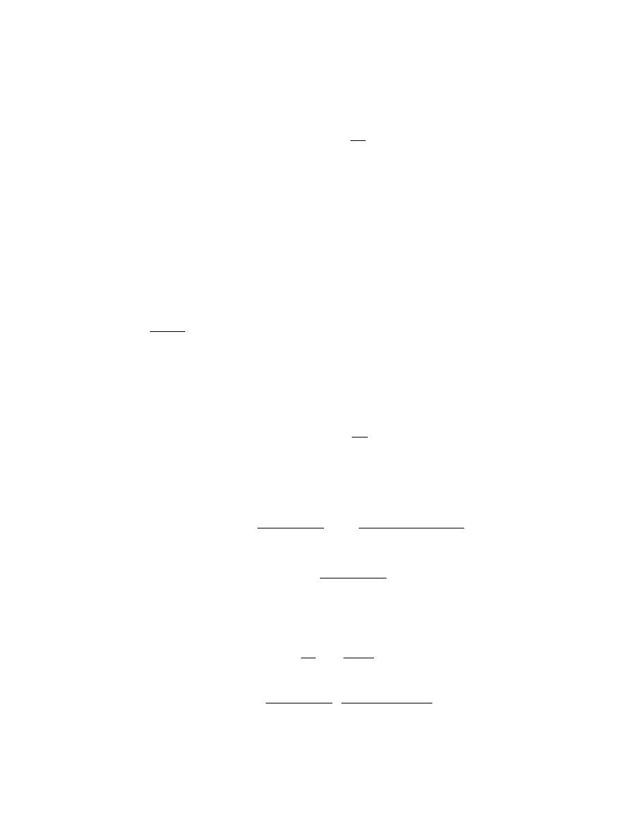
Excerpts from this work may be reproduced by instructors for distribution on a not-for-profit basis for testing or instructional purposes only to
students enrolled in courses for which the textbook has been adopted. Any other reproduction or translation of this work beyond that permitted
by Sections 107 or 108 of the 1976 United States Copyright Act without the permission of the copyright owner is unlawful.
14.29 The permeability coefficient of a type of small gas molecule in a polymer is dependent on absolute
temperature according to the following equation:
P
M
= P
M
0
exp
−
Q
p
RT
where
P
M
0
and Q
p
are constants for a given gas-polymer pair. Consider the diffusion of hydrogen through a
poly(dimethyl siloxane) (PDMSO) sheet 20 mm thick. The hydrogen pressures at the two faces are 10 kPa and 1
kPa, which are maintained constant. Compute the diffusion flux [in (cm
3
STP)/cm
2
–s]
at 350 K. For this diffusion
system
P
M
0
= 1.45 × 10
−8
(cm
3
STP)(cm)/cm
2
- s - Pa
Q
p
= 13.7 kJ/mol
Also, assume a condition of steady state diffusion
Solution
This problem asks that we compute the diffusion flux at 350 K for hydrogen in poly(dimethyl siloxane)
(PDMSO). It is first necessary to compute the value of the permeability coefficient at 350 K. The temperature
dependence of P
M
is given in the problem statement, as follows:
P
M
= P
M
0
exp
−
Q
p
RT
And, incorporating values provided for the constants P
M
0
and Q
p
, we get
P
M
= 1.45
× 10
-8
(cm
3
STP)(cm)
cm
2
- s - Pa
exp −
13, 700 J/mol
(8.31 J/mol - K)(350 K)
= 1.31 × 10
−10
(cm
3
STP)(cm)
cm
2
- s - Pa
And, using Equation 14.9, the diffusion flux is equal to
J = P
M
∆P
∆x
= P
M
P
2
− P
1
∆x
= 1.31 × 10
-10
(cm
3
STP)(cm)
cm
2
- s - Pa
10, 000 Pa - 1, 000 Pa
2.0 cm

Excerpts from this work may be reproduced by instructors for distribution on a not-for-profit basis for testing or instructional purposes only to
students enrolled in courses for which the textbook has been adopted. Any other reproduction or translation of this work beyond that permitted
by Sections 107 or 108 of the 1976 United States Copyright Act without the permission of the copyright owner is unlawful.
= 5.90 × 10
-7
(cm
3
STP)
cm
2
- s

Excerpts from this work may be reproduced by instructors for distribution on a not-for-profit basis for testing or instructional purposes only to
students enrolled in courses for which the textbook has been adopted. Any other reproduction or translation of this work beyond that permitted
by Sections 107 or 108 of the 1976 United States Copyright Act without the permission of the copyright owner is unlawful.
CHAPTER 15
CHARACTERISTICS, APPLICATIONS, AND PROCESSING OF POLYMERS
PROBLEM SOLUTIONS
Stress-Strain Behavior
15.1 From the stress–strain data for poly(methyl methacrylate) shown in Figure 15.3, determine the
modulus of elasticity and tensile strength at room temperature [20°C (68°F)], and compare these values with those
given in Table 15.1.
Solution
From Figure 15.3, the elastic modulus is the slope in the elastic linear region of the 20
°C curve, which is
E =
∆ (stress)
∆ (strain)
=
30 MPa
− 0 MPa
9
× 10
−3
− 0
= 3.3 GPa (483,000 psi)
The value range cited in Table 15.1 is 2.24 to 3.24 GPa (325,000 to 470,000 psi). Thus, the plotted value is a little
on the high side.
The tensile strength corresponds to the stress at which the curve ends, which is 52 MPa (7500 psi). This
value lies within the range cited in Table 15.1—48.3 to 72.4 MPa (7000 to 10,500 psi).

Excerpts from this work may be reproduced by instructors for distribution on a not-for-profit basis for testing or instructional purposes only to
students enrolled in courses for which the textbook has been adopted. Any other reproduction or translation of this work beyond that permitted
by Sections 107 or 108 of the 1976 United States Copyright Act without the permission of the copyright owner is unlawful.
15.2 Compute the elastic moduli for the following polymers, whose stress-strain behaviors may be
observed in the “Tensile Tests” module of Virtual Materials Science and Engineering (VMSE): (a) high-density
polyethylene, (b) nylon, and (c) phenol-formaldehyde (bakelite). How do these values compare with those presented
in Table 15.1 for the same polymers?
Solution
The elastic modulus is the slope in the linear elastic region (Equation 6.10) as
E =
∆ σ
∆ ε
=
σ
2
− σ
1
ε
2
− ε
1
Since all the stress-strain curves pass through the origin, we make take
σ
1
= 0 and
ε
1
= 0. Determinations of
σ
2
and
ε
2
are possible by moving the cursor to some arbitrary point in the linear region of the curve and then reading
corresponding values in the “Stress” and “Strain” windows that are located below the plot.
(a) For high-density polyethylene, we selected
σ
2
= 6.0 MPa with its corresponding
ε
2
= 0.0152.
Therefore,
E =
σ
2
− σ
1
ε
2
− ε
1
=
6.0 MPa
− 0 MPa
0.0152
− 0
= 395 MPa = 0.395 GPa
The elastic modulus (average) for high-density polyethylene given in Table 15.1 is 1.08 GPa, which is
significantly higher than this value.
(b) For nylon, we selected
σ
2
= 24.3 MPa with its corresponding
ε
2
= 0.0085. Therefore,
E =
σ
2
− σ
1
ε
2
− ε
1
=
24.3 MPa
− 0 MPa
0.0085
− 0
= 2860 MPa = 2.86 GPa
The elastic modulus range for nylon 6,6 given in Table 15.1 is 1.58 GPa to 3.80 GPa; therefore, the value
for the VMSE nylon lies within this range.

Excerpts from this work may be reproduced by instructors for distribution on a not-for-profit basis for testing or instructional purposes only to
students enrolled in courses for which the textbook has been adopted. Any other reproduction or translation of this work beyond that permitted
by Sections 107 or 108 of the 1976 United States Copyright Act without the permission of the copyright owner is unlawful.
(c) For phenol-formaldehyde (bakelite), we selected
σ
2
= 33.0 MPa with its corresponding
ε
2
= 0.0068.
Therefore,
E =
σ
2
− σ
1
ε
2
− ε
1
=
33.0 MPa
− 0 MPa
0.0068
− 0
= 4850 MPa = 4.85 GPa
The elastic modulus range for the phenol-formaldehyde given in Table 15.1 is 2.76 GPa to 4.83 GPa;
therefore, this value for the VMSE phenol-formaldehyde lies just above the maximum value for this range.

Excerpts from this work may be reproduced by instructors for distribution on a not-for-profit basis for testing or instructional purposes only to
students enrolled in courses for which the textbook has been adopted. Any other reproduction or translation of this work beyond that permitted
by Sections 107 or 108 of the 1976 United States Copyright Act without the permission of the copyright owner is unlawful.
15.3 For the nylon polymer, whose stress strain behavior may be observed in the “Tensile Tests” module
of Virtual Materials Science and Engineering (VMSE), determine the following:
(a) the yield strength, and
(b) the approximate ductility, in percent elongation.
How do these values compare with those for the nylon material presented in Table 15.1?
Solution
(a) The yield strength corresponds to the first maximum (just beyond the initial linear-elastic region) of the
stress-strain curve. This reading in the stress window located below the plot as the curser point is dragged along the
stress-strain curve is 84 MPa.
(b) The approximate percent elongation corresponds to the strain at fracture multiplied by 100 (i.e.,
44.5%) minus the maximum elastic strain (i.e., value of strain at which the linearity of the curve ends multiplied by
100—in this case about 4%); this gives a value of about 40%EL.
For nylon 6,6, the range of values of yield strength presented in Table 15.1 is 44.8 MPa to 82.8 MPa;
therefore, the value for the VMSE nylon lies slightly above the upper value. The ductility range for nylon 6,6 is
15%EL to 300%EL; therefore, our value (40%EL) lies within this range.

Excerpts from this work may be reproduced by instructors for distribution on a not-for-profit basis for testing or instructional purposes only to
students enrolled in courses for which the textbook has been adopted. Any other reproduction or translation of this work beyond that permitted
by Sections 107 or 108 of the 1976 United States Copyright Act without the permission of the copyright owner is unlawful.
15.4 For the phenol-formaldehyde (Bakelite) polymer, whose stress strain behavior may be observed in
the “Tensile Tests” module of Virtual Materials Science and Engineering (VMSE), determine the following:
(a) the tensile strength, and
(b) the approximate ductility, in percent elongation.
How do these values compare with those for the phenol-formaldehyde material presented in Table 15.1?
Solution
(a) The tensile strength corresponds to the stress at which fracture occurs. This reading in the stress
window located below the plot as the curser point is dragged along the stress-strain curve is 52 MPa.
(b) The approximate percent elongation corresponds to the strain at fracture multiplied by 100 (i.e.,
1.29%) minus the maximum elastic strain (i.e., value of strain at which the linearity of the curve ends multiplied by
100—in this case about 1%); this gives a value of about 0.3%EL.
For phenol-formaldehyde, the range of values of tensile strength presented in Table 15.1 is 34.5 MPa to
62.1 MPa; therefore, the value for the VMSE material (52 MPa) lies within this range. The ductility range for
phenol-formaldehyde is 1.5%EL to 2.0%EL; therefore, our value (0.3%EL) lies below the lower limit.

Excerpts from this work may be reproduced by instructors for distribution on a not-for-profit basis for testing or instructional purposes only to
students enrolled in courses for which the textbook has been adopted. Any other reproduction or translation of this work beyond that permitted
by Sections 107 or 108 of the 1976 United States Copyright Act without the permission of the copyright owner is unlawful.
Viscoelastic Deformation
15.5 In your own words, briefly describe the phenomenon of viscoelasticity.
The explanation of viscoelasticity is given in Section 15.4.

Excerpts from this work may be reproduced by instructors for distribution on a not-for-profit basis for testing or instructional purposes only to
students enrolled in courses for which the textbook has been adopted. Any other reproduction or translation of this work beyond that permitted
by Sections 107 or 108 of the 1976 United States Copyright Act without the permission of the copyright owner is unlawful.
15.6 For some viscoelastic polymers that are subjected to stress relaxation tests, the stress decays with
time according to
σ(t) = σ(0) exp −
t
τ
(15.10)
where σ(t) and σ(0) represent the time-dependent and initial (i.e., time = 0) stresses, respectively, and t and τ denote
elapsed time and the relaxation time; τ is a time-independent constant characteristic of the material. A specimen of
some viscoelastic polymer the stress relaxation of which obeys Equation 15.10 was suddenly pulled in tension to a
measured strain of 0.6; the stress necessary to maintain this constant strain was measured as a function of time.
Determine E
r
(10) for this material if the initial stress level was 2.76 MPa (400 psi), which dropped to 1.72 MPa
(250 psi) after 60 s.
Solution
This problem asks for a determination of the relaxation modulus of a viscoelastic material, which behavior
is according to Equation 15.10--i.e.,
σ(t) = σ(0) exp −
t
τ
We want to determine
σ(10), but it is first necessary to compute τ from the data provided in the problem statement.
Thus, solving for
τ from the above expression,
τ =
− t
ln
σ(t)
σ(0)
=
− 60 s
ln
1.72 MPa
2.76 MPa
= 127 s
Therefore,
σ(10) = (2.76 MPa) exp −
10 s
127 s
= 2.55 MPa
Now, using Equation 15.1
E
r
(10) =
σ (10)
ε
0
=
2.55 MPa
0.6
= 4.25 MPa (616 psi)
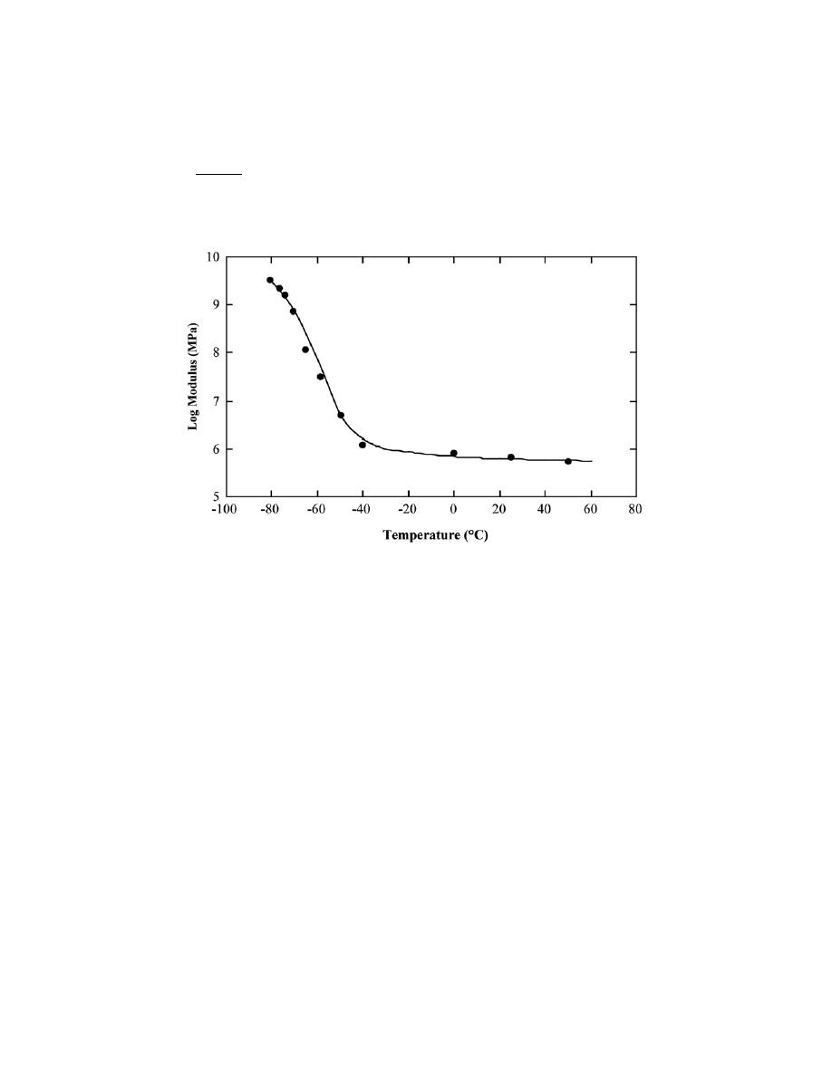
Excerpts from this work may be reproduced by instructors for distribution on a not-for-profit basis for testing or instructional purposes only to
students enrolled in courses for which the textbook has been adopted. Any other reproduction or translation of this work beyond that permitted
by Sections 107 or 108 of the 1976 United States Copyright Act without the permission of the copyright owner is unlawful.
15.7 In Figure 15.28, the logarithm of E
r
(t) versus the logarithm of time is plotted for polyisobutylene at a
variety of temperatures. Make a plot of E
r
(10) versus temperature and then estimate its T
g
.
Solution
Below is plotted the logarithm of E
r
(10) versus temperature.
The glass-transition temperature is that temperature corresponding to the abrupt decrease in log E
r
(10), which for
this polyisobutylene material is about -60
°C.

Excerpts from this work may be reproduced by instructors for distribution on a not-for-profit basis for testing or instructional purposes only to
students enrolled in courses for which the textbook has been adopted. Any other reproduction or translation of this work beyond that permitted
by Sections 107 or 108 of the 1976 United States Copyright Act without the permission of the copyright owner is unlawful.
15.8 On the basis of the curves in Figure 15.5, sketch schematic strain–time plots for the following
polystyrene materials at the specified temperatures:
(a) Amorphous at 120
°C
(b) Crosslinked at 150
°C
(c) Crystalline at 230
°C
(d) Crosslinked at 50
°C
Solution
(a) Amorphous polystyrene at 120
°C behaves a rubbery material (Figure 15.8, curve C); therefore, the
strain-time behavior would be as Figure 15.5c.
(b) Crosslinked polystyrene at 150
°C behaves as a viscoelastic material (Figure 15.8, curve B); therefore,
the strain-time behavior will be as Figure 15.5c.
(c) Crystalline polystyrene at 230
°C behaves as a viscous liquid (Figure 15.8, curve A); therefore, the
strain-time behavior will be as Figure 15.5d.
(d) Crosslinked polystyrene at 50
°C behaves in a glassy manner (Figure 15.8, curve B); therefore, the
strain-time behavior will be as Figure 15.5b.

Excerpts from this work may be reproduced by instructors for distribution on a not-for-profit basis for testing or instructional purposes only to
students enrolled in courses for which the textbook has been adopted. Any other reproduction or translation of this work beyond that permitted
by Sections 107 or 108 of the 1976 United States Copyright Act without the permission of the copyright owner is unlawful.
15.9 (a) Contrast the manner in which stress relaxation and viscoelastic creep tests are conducted.
(b) For each of these tests, cite the experimental parameter of interest and how it is determined.
Solution
(a) Stress relaxation tests are conducted by rapidly straining the material elastically in tension, holding the
strain level constant, and then measuring the stress as a function of time. For viscoelastic creep tests, a stress
(usually tensile) is applied instantaneously and maintained constant while strain is measured as a function of time.
(b) The experimental parameters of interest from the stress relaxation and viscoelastic creep tests are the
relaxation modulus and creep modulus (or creep compliance), respectively. The relaxation modulus is the ratio of
stress measured after 10 s and strain (Equation 15.1); creep modulus is the ratio of stress and strain taken at a
specific time (Equation 15.2).
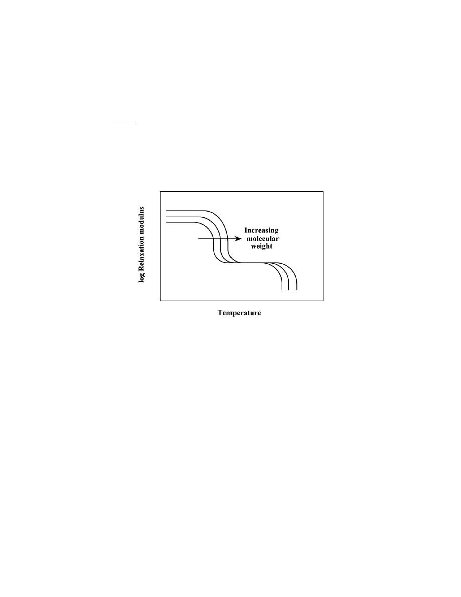
Excerpts from this work may be reproduced by instructors for distribution on a not-for-profit basis for testing or instructional purposes only to
students enrolled in courses for which the textbook has been adopted. Any other reproduction or translation of this work beyond that permitted
by Sections 107 or 108 of the 1976 United States Copyright Act without the permission of the copyright owner is unlawful.
15.10 Make two schematic plots of the logarithm of relaxation modulus versus temperature for an
amorphous polymer (curve C in Figure 15.8).
(a) On one of these plots demonstrate how the behavior changes with increasing molecular weight.
(b) On the other plot, indicate the change in behavior with increasing crosslinking.
Solution
(a) This portion of the problem calls for a plot of log E
r
(10) versus temperature demonstrating how the
behavior changes with increased molecular weight. Such a plot is given below. Increasing molecular weight
increases both glass-transition and melting temperatures.
(b) We are now called upon to make a plot of log E
r
(10) versus temperature demonstrating how the
behavior changes with increased crosslinking. Such a plot is given below. Increasing the degree of crosslinking
will increase the modulus in both glassy and rubbery regions.
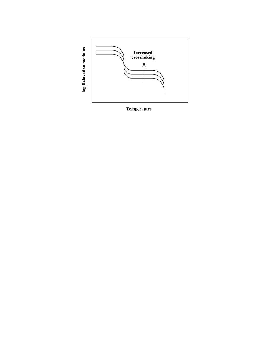
Excerpts from this work may be reproduced by instructors for distribution on a not-for-profit basis for testing or instructional purposes only to
students enrolled in courses for which the textbook has been adopted. Any other reproduction or translation of this work beyond that permitted
by Sections 107 or 108 of the 1976 United States Copyright Act without the permission of the copyright owner is unlawful.
Fracture of Polymers
Miscellaneous Mechanical Considerations
15.11 For thermoplastic polymers, cite five factors that favor brittle fracture.
Solution
For thermoplastic polymers, five factors that favor brittle fracture are as follows: (1) a reduction in
temperature, (2) an increase in strain rate, (3) the presence of a sharp notch, (4) increased specimen thickness, and
(5) modifications of the polymer structure.

Excerpts from this work may be reproduced by instructors for distribution on a not-for-profit basis for testing or instructional purposes only to
students enrolled in courses for which the textbook has been adopted. Any other reproduction or translation of this work beyond that permitted
by Sections 107 or 108 of the 1976 United States Copyright Act without the permission of the copyright owner is unlawful.
15.12 (a) Compare the fatigue limits for polystyrene (Figure 15.11) and the cast iron for which fatigue
data are given in Problem 8.20.
(b) Compare the fatigue strengths at 10
6
cycles for poly(ethylene terephthalate) (PET, Figure 15.11) and
red brass (Figure 8.34).
Solution
(a) The fatigue limits for polystyrene and the cast iron are 10.5 MPa (1500 psi) and 193 MPa (28,000 psi),
respectively.
(b) At 10
6
cycles, the fatigue strengths of PET and red brass are 15 MPa (2175 psi) and 115 MPa (16,700
psi ), respectively.

Excerpts from this work may be reproduced by instructors for distribution on a not-for-profit basis for testing or instructional purposes only to
students enrolled in courses for which the textbook has been adopted. Any other reproduction or translation of this work beyond that permitted
by Sections 107 or 108 of the 1976 United States Copyright Act without the permission of the copyright owner is unlawful.
Deformation of Semicrystalline Polymers
15.13 In your own words, describe the mechanisms by which semicrystalline polymers (a) elastically
deform and (b) plastically deform, and (c) by which elastomers elastically deform.
(a) and (b) The mechanisms by which semicrystalline polymers elastically and plastically deform are
described in Section 15.7.
(c) The explanation of the mechanism by which elastomers elastically deform is provided in Section 15.9.

Excerpts from this work may be reproduced by instructors for distribution on a not-for-profit basis for testing or instructional purposes only to
students enrolled in courses for which the textbook has been adopted. Any other reproduction or translation of this work beyond that permitted
by Sections 107 or 108 of the 1976 United States Copyright Act without the permission of the copyright owner is unlawful.
Factors That Influence the Mechanical Properties of Semicrystalline
Polymers
Deformation of Elastomers
15.14 Briefly explain how each of the following influences the tensile modulus of a semicrystalline
polymer and why:
(a) Molecular weight
(b) Degree of crystallinity
(c) Deformation by drawing
(d) Annealing of an undeformed material
(f) Annealing of a drawn material
Solution
(a) The tensile modulus is not directly influenced by a polymer's molecular weight.
(b) Tensile modulus increases with increasing degree of crystallinity for semicrystalline polymers. This is
due to enhanced secondary interchain bonding which results from adjacent aligned chain segments as percent
crystallinity increases. This enhanced interchain bonding inhibits relative interchain motion.
(c) Deformation by drawing also increases the tensile modulus. The reason for this is that drawing
produces a highly oriented molecular structure, and a relatively high degree of interchain secondary bonding.
(d) When an undeformed semicrystalline polymer is annealed below its melting temperature, the tensile
modulus increases.
(e) A drawn semicrystalline polymer that is annealed experiences a decrease in tensile modulus as a result
of a reduction in chain-induced crystallinity, and a reduction in interchain bonding forces.

Excerpts from this work may be reproduced by instructors for distribution on a not-for-profit basis for testing or instructional purposes only to
students enrolled in courses for which the textbook has been adopted. Any other reproduction or translation of this work beyond that permitted
by Sections 107 or 108 of the 1976 United States Copyright Act without the permission of the copyright owner is unlawful.
15.15 Briefly explain how each of the following influences the tensile or yield strength of a semicrystalline
polymer and why:
(a) Molecular weight
(b) Degree of crystallinity
(c) Deformation by drawing
(d) Annealing of an undeformed material
Solution
(a) The tensile strength of a semicrystalline polymer increases with increasing molecular weight. This
effect is explained by increased chain entanglements at higher molecular weights.
(b) Increasing the degree of crystallinity of a semicrystalline polymer leads to an enhancement of the
tensile strength. Again, this is due to enhanced interchain bonding and forces; in response to applied stresses,
interchain motions are thus inhibited.
(c) Deformation by drawing increases the tensile strength of a semicrystalline polymer. This effect is due
to the highly oriented chain structure that is produced by drawing, which gives rise to higher interchain secondary
bonding forces.
(d) Annealing an undeformed semicrystalline polymer produces an increase in its tensile strength.

Excerpts from this work may be reproduced by instructors for distribution on a not-for-profit basis for testing or instructional purposes only to
students enrolled in courses for which the textbook has been adopted. Any other reproduction or translation of this work beyond that permitted
by Sections 107 or 108 of the 1976 United States Copyright Act without the permission of the copyright owner is unlawful.
15.16 Normal butane and isobutane have boiling temperatures of –0.5 and –12.3°C (31.1 and 9.9°F),
respectively. Briefly explain this behavior on the basis of their molecular structures, as presented in Section 14.2.
Solution
Normal butane has a higher melting temperature as a result of its molecular structure (Section 14.2). There
is more of an opportunity for van der Waals bonds to form between two molecules in close proximity to one another
than for isobutane because of the linear nature of each normal butane molecule.
Excerpts from this work may be reproduced by instructors for distribution on a not-for-profit basis for testing or instructional purposes only to
students enrolled in courses for which the textbook has been adopted. Any other reproduction or translation of this work beyond that permitted
by Sections 107 or 108 of the 1976 United States Copyright Act without the permission of the copyright owner is unlawful.
15.17 The tensile strength and number-average molecular weight for two poly(methyl methacrylate)
materials are as follows:
Tensile Strength
(MPa)
Number-Average
Molecular Weight (g/mol)
107
40,000
170
60,000
Estimate the tensile strength at a number-average molecular weight of 30,000 g/mol.
Solution
This problem gives us the tensile strengths and associated number-average molecular weights for two
poly(methyl methacrylate) materials and then asks that we estimate the tensile strength for
M
n
= 30,000 g/mol.
Equation 15.3 cites the dependence of the tensile strength on
M
n
. Thus, using the data provided in the problem
statement, we may set up two simultaneous equations from which it is possible to solve for the two constants TS
∞
and A. These equations are as follows:
107 MPa = TS
∞
−
A
40, 000 g / mol
170 MPa = TS
∞
−
A
60, 000 g / mol
Thus, the values of the two constants are: TS
∞
= 296 MPa and A = 7.56
× 10
6
MPa-g/mol. Substituting these
values into Equation 15.3 for
M
n
= 30,000 g/mol leads to
TS = TS
∞
−
A
30, 000 g / mol
= 296 MPa
−
7.56
× 10
6
MPa - g / mol
30, 000 g / mol
= 44 MPa
Excerpts from this work may be reproduced by instructors for distribution on a not-for-profit basis for testing or instructional purposes only to
students enrolled in courses for which the textbook has been adopted. Any other reproduction or translation of this work beyond that permitted
by Sections 107 or 108 of the 1976 United States Copyright Act without the permission of the copyright owner is unlawful.
15.18 The tensile strength and number-average molecular weight for two polyethylene materials are as
follows:
Tensile Strength
(MPa)
Number-Average
Molecular Weight (g/mol)
85
12,700
150
28,500
Estimate the number-average molecular weight that is required to give a tensile strength of 195 MPa.
Solution
This problem gives us the tensile strengths and associated number-average molecular weights for two
polyethylene materials and then asks that we estimate the
M
n
that is required for a tensile strength of 195 MPa.
Equation 15.3 cites the dependence of the tensile strength on
M
n
. Thus, using the data provided in the problem
statement, we may set up two simultaneous equations from which it is possible to solve for the two constants TS
∞
and A. These equations are as follows:
85 MPa = TS
∞
−
A
12, 700 g / mol
150 MPa = TS
∞
−
A
28, 500 g / mol
Thus, the values of the two constants are: TS
∞
= 202 MPa and A = 1.489
× 10
6
MPa-g/mol. Solving for
M
n
in
Equation 15.3 and substituting TS = 195 MPa as well as the above values for TS
∞
and A leads to
M
n
=
A
TS
∞
− TS
=
1.489
× 10
6
MPa - g / mol
202 MPa
− 195 MPa
= 213, 000 g/mol

Excerpts from this work may be reproduced by instructors for distribution on a not-for-profit basis for testing or instructional purposes only to
students enrolled in courses for which the textbook has been adopted. Any other reproduction or translation of this work beyond that permitted
by Sections 107 or 108 of the 1976 United States Copyright Act without the permission of the copyright owner is unlawful.
15.19 For each of the following pairs of polymers, do the following: (1) state whether or not it is possible
to decide whether one polymer has a higher tensile modulus than the other; (2) if this is possible, note which has the
higher tensile modulus and then cite the reason(s) for your choice; and (3) if it is not possible to decide, then state
why.
(a) Random acrylonitrile-butadiene copolymer with 10% of possible sites crosslinked; alternating
acrylonitrile-butadiene copolymer with 5% of possible sites crosslinked
(b) Branched and syndiotactic polypropylene with a degree of polymerization of 5000; linear and isotactic
polypropylene with a degree of polymerization of 3000
(c) Branched polyethylene with a number-average molecular weight of 250,000 g/mol; linear and isotactic
poly(vinyl chloride) with a number-average molecular weight of 200,000 g/mol
Solution
For each of four pairs of polymers, we are to do the following: (1) determine whether or not it is possible to decide
which has the higher tensile modulus; (2) if so, note which has the higher tensile modulus and then state the
reasons for this choice; and (3) if it is not possible to decide, then state why.
(a) No, it is not possible. The random acrylonitrile-butadiene copolymer will tend to a lower degree of
crystallinity than the alternating acrylonitrile-butadiene copolymer inasmuch as random copolymers don’t normally
crystallize. On this basis only, the alternating material would have a higher modulus inasmuch as tensile modulus
increases with degree of crystallinity. On the other hand, the random copolymer has a higher degree of crosslinking
(10% versus 5% for the alternating copolymer), and, on this basis only would have the higher tensile modulus—an
increase in crosslinking leads to an increase in E. Thus, this determination is not possible; with regard to degree of
crystallinity the alternating material has the higher E, whereas the random copolymer would have a higher E value
on the basis of degree of crosslinking.
(b) Yes, it is possible. The linear and isotactic polypropylene will have a greater tensile modulus. Linear
polymers are more likely to crystallize that branched ones. The likelihood of crystallization for both syndiotactic
and isotactic polypropylene is about the same, and, therefore, degree is crystallization is not a factor. Furthermore,
tensile modulus is relatively insensitive to degree of polymerization (i.e., molecular weight)—the fact that branched
PP has the higher molecular weight is not important.
(c) No, it is not possible. Linear polymers have higher degrees of crystallization (and higher tensile
moduli) than branched polymers—on this basis, the PVC material should have the higher value of E. On the other
hand, PVC has a more complex repeat unit structure than does polyethylene, which means that, on this basis, the PE
would have a higher degree of crystallinity and also a greater tensile modulus. Also, tensile modulus is relatively
independent of number-average molecular weight. Therefore, this determination is not possible since it is not
possible to determine which of the two materials has the greater degree of crystallinity.

Excerpts from this work may be reproduced by instructors for distribution on a not-for-profit basis for testing or instructional purposes only to
students enrolled in courses for which the textbook has been adopted. Any other reproduction or translation of this work beyond that permitted
by Sections 107 or 108 of the 1976 United States Copyright Act without the permission of the copyright owner is unlawful.
15.20 For each of the following pairs of polymers, do the following: (1) state whether or not it is possible
to decide whether one polymer has a higher tensile strength than the other; (2) if this is possible, note which has the
higher tensile strength and then cite the reason(s) for your choice; and (3) if it is not possible to decide, then state
why.
(a) Syndiotactic polystyrene having a number-average molecular weight of 600,000 g/mol; atactic
polystyrene having a number-average molecular weight of 500,000 g/mol
(b) Random acrylonitrile-butadiene copolymer with 10% of possible sites crosslinked; block acrylonitrile-
butadiene copolymer with 5% of possible sites crosslinked
(c) Network polyester; lightly branched polypropylene
Solution
For each of three pairs of polymers, we are to do the following: (1) determine whether or not it is possible
to decide which has the higher tensile strength; (2) if it is possible, then note which has the higher tensile strength
and then state the reasons for this choice; and (3) if it is not possible to decide, to state why.
(a) Yes it is possible. The syndiotactic polystyrene has the higher tensile strength. Syndiotactic polymers
are more likely to crystallize than atactic ones; the greater the crystallinity, the higher the tensile strength.
Furthermore, the syndiotactic also has a higher molecular weight; increasing molecular weight also enhances the
strength.
(b) No it is not possible. The random acrylonitrile-butadiene copolymer has more crosslinking; increased
crosslinking leads to an increase in strength. However, the block copolymeric material will most likely have a
higher degree of crystallinity; and increasing crystallinity improves the strength.
(c) Yes it is possible. The network polyester will display a greater tensile strength. Relative chain motion
is much more restricted than for the lightly branched polypropylene since there are many more of the strong
covalent bonds for the network structure.
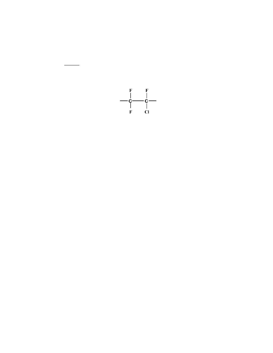
Excerpts from this work may be reproduced by instructors for distribution on a not-for-profit basis for testing or instructional purposes only to
students enrolled in courses for which the textbook has been adopted. Any other reproduction or translation of this work beyond that permitted
by Sections 107 or 108 of the 1976 United States Copyright Act without the permission of the copyright owner is unlawful.
15.21 Would you expect the tensile strength of polychlorotrifluoroethylene to be greater than, the same as,
or less than that of a polytetrafluoroethylene specimen having the same molecular weight and degree of
crystallinity? Why?
Solution
The strength of a polychlorotrifluoroethylene having the repeat unit structure
will be greater than for a polytetrafluoroethylene having the same molecular weight and degree of crystallinity. The
replacement of one fluorine atom within the PTFE repeat unit with a chlorine atom leads to a higher interchain
attraction, and, thus, a stronger polymer. Furthermore, poly(vinyl chloride) is stronger than polyethylene (Table
15.1) for the same reason.
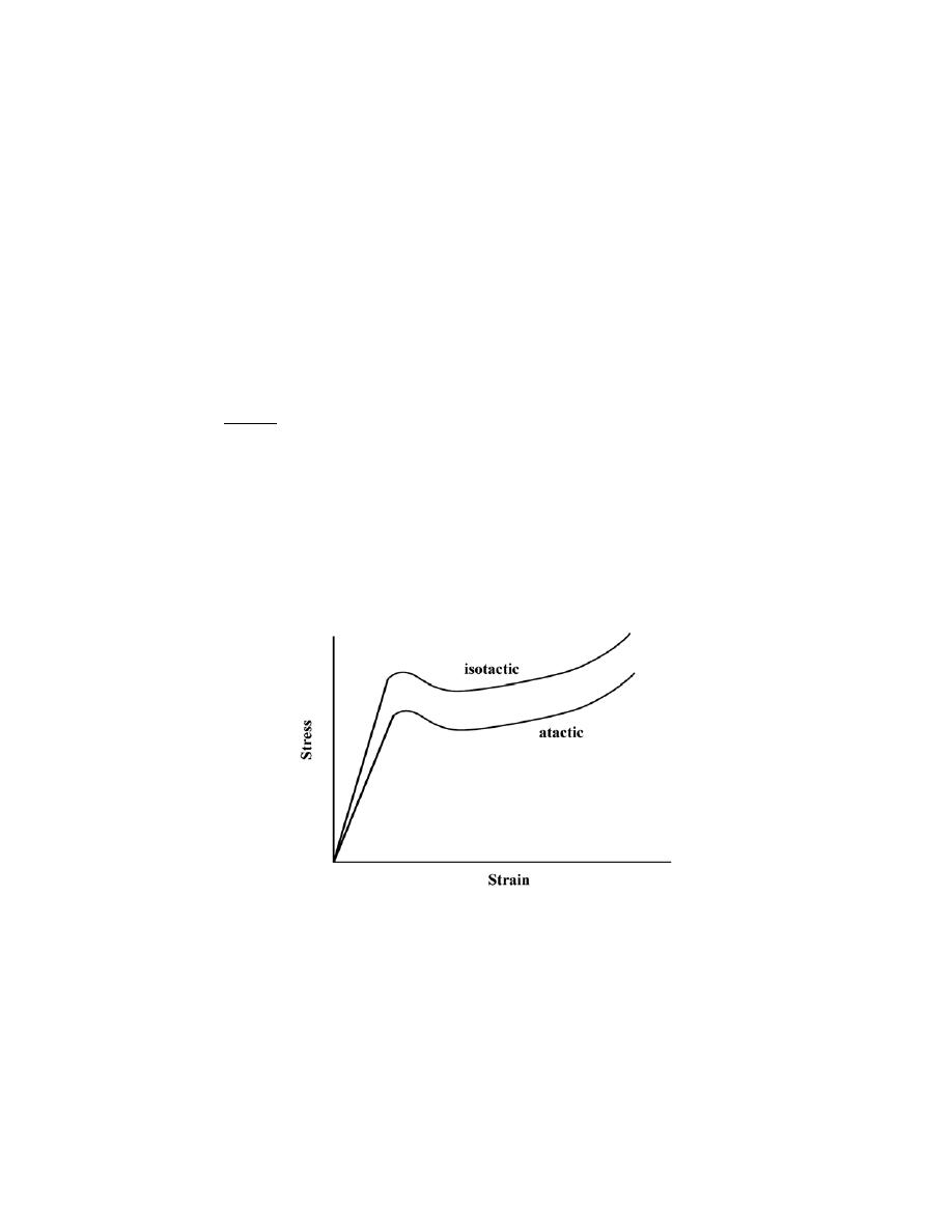
Excerpts from this work may be reproduced by instructors for distribution on a not-for-profit basis for testing or instructional purposes only to
students enrolled in courses for which the textbook has been adopted. Any other reproduction or translation of this work beyond that permitted
by Sections 107 or 108 of the 1976 United States Copyright Act without the permission of the copyright owner is unlawful.
15.22 For each of the following pairs of polymers, plot and label schematic stress–strain curves on the
same graph [i.e., make separate plots for parts (a), (b), and (c)].
(a) Isotactic and linear polypropylene having a weight-average molecular weight of 120,000 g/mol; atactic
and linear polypropylene having a weight-average molecular weight of 100,000 g/mol
(b) Branched poly(vinyl chloride) having a degree of polymerization of 2000; heavily crosslinked
poly(vinyl chloride) having a degree of polymerization of 2000
(c) Poly(styrene-butadiene) random copolymer having a number-average molecular weight of 100,000
g/mol and 10% of the available sites crosslinked and tested at 20
°C; poly(styrene-butadiene) random copolymer
having a number-average molecular weight of 120,000 g/mol and 15% of the available sites crosslinked and tested
at -85
°C. Hint: poly(styrene-butadiene) copolymers may exhibit elastomeric behavior.
Solution
(a) Shown below are the stress-strain curves for the two polypropylene materials. These materials will
display the stress-strain behavior of a normal plastic, curve B in Figure 15.1. However, the isotactic/linear will have
a higher degree of crystallinity (since isotactic are more likely to crystallize than atactic/linear), and therefore, will
have a higher tensile modulus and strength. Furthermore, the isotactic/linear also has a higher molecular weight
which also leads to an increase in strength.
(b) Shown below are the stress-strain curves for the two polyvinyl chloride materials. The branched PVC
will probably display the stress-strain behavior of a plastic, curve B in Figure 15.1. However, the heavily
crosslinked PVC will undoubtedly have a higher tensile modulus, and, also a higher strength, and will most likely
fail in a brittle manner--as curve A, Figure 15.1; these are the typical characteristics of a heavily crosslinked
polymer.
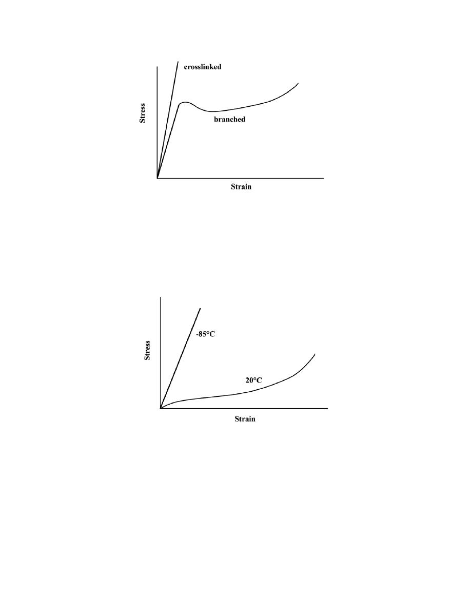
Excerpts from this work may be reproduced by instructors for distribution on a not-for-profit basis for testing or instructional purposes only to
students enrolled in courses for which the textbook has been adopted. Any other reproduction or translation of this work beyond that permitted
by Sections 107 or 108 of the 1976 United States Copyright Act without the permission of the copyright owner is unlawful.
(c) Shown below are the stress-strain curves for the two poly(styrene-butadiene) random copolymers. The
copolymer tested at 20
°C will display elastomeric behavior (curve C of Figure 15.1) inasmuch as it is a random
copolymer that is lightly crosslinked; furthermore, the temperature of testing is above its glass transition
temperature. On the other hand, since -85
°C is below the glass transition temperature of the poly(styrene-
butadiene) copolymer, the stress-strain behavior under these conditions is as curve A of Figure 15.1.

Excerpts from this work may be reproduced by instructors for distribution on a not-for-profit basis for testing or instructional purposes only to
students enrolled in courses for which the textbook has been adopted. Any other reproduction or translation of this work beyond that permitted
by Sections 107 or 108 of the 1976 United States Copyright Act without the permission of the copyright owner is unlawful.
15.23 List the two molecular characteristics that are essential for elastomers.
Solution
Two molecular characteristics essential for elastomers are: (1) they must be amorphous, having chains that
are extensively coiled and kinked in the unstressed state; and (2) there must be some crosslinking.

Excerpts from this work may be reproduced by instructors for distribution on a not-for-profit basis for testing or instructional purposes only to
students enrolled in courses for which the textbook has been adopted. Any other reproduction or translation of this work beyond that permitted
by Sections 107 or 108 of the 1976 United States Copyright Act without the permission of the copyright owner is unlawful.
15.24 Which of the following would you expect to be elastomers and which thermosetting polymers at
room temperature? Justify each choice.
(a) Epoxy having a network structure
(b) Lightly crosslinked poly(styrene-butadiene) random copolymer that has a glass-transition temperature
of -50
°C
(c) Lightly branched and semicrystalline polytetrafluoroethylene that has a glass-transition temperature of
-100
°C
(d) Heavily crosslinked poly(ethylene-propylene) random copolymer that has a glass-transition
temperature of 0
°C
(e) Thermoplastic elastomer that has a glass-transition temperature of 75
°C
Solution
This question asks us to choose from a list of materials those that would be expected to be elastomers and
those that would be thermosetting polymers.
(a) Epoxy having a network structure will be a thermoset polymer since it has a network structure. It
would not be an elastomer since it does not have a crosslinked chain structure.
(b) A lightly crosslinked poly(styrene-butadiene) random copolymer that has a glass-transition temperature
of -50
°C will be an elastomer since it 1) is a random copolymer, 2) is lightly crosslinked, and 3) is being used at a
temperature above its glass transition. All three of these criteria are requisites for an elastomer.
(c) Lightly branched and semicrystalline PTFE would be neither an elastomer nor a thermoset. It is not
crosslinked nor does it have a network structure.
(d) A heavily crosslinked poly(ethylene-propylene) random copolymer would be a thermoset inasmuch as
it is heavily crosslinked.
(e) A thermoplastic elastomer that has a glass-transition temperature of 75
°C is neither an elastomer nor a
thermoset. Since it is a thermoplastic it is not a thermoset. Furthermore, room temperature is below its glass-
transition temperature, and, therefore, it will not display elastomeric behavior.

Excerpts from this work may be reproduced by instructors for distribution on a not-for-profit basis for testing or instructional purposes only to
students enrolled in courses for which the textbook has been adopted. Any other reproduction or translation of this work beyond that permitted
by Sections 107 or 108 of the 1976 United States Copyright Act without the permission of the copyright owner is unlawful.
15.25 Ten kilogram of polybutadiene is vulcanized with 4.8 kg sulfur. What fraction of the possible
crosslink sites is bonded to sulfur crosslinks, assuming that, on the average, 4.5 sulfur atoms participate in each
crosslink?
Solution
This problem asks that we compute the fraction of possible crosslink sites in 10 kg of polybutadiene when
4.8 kg of S is added, assuming that, on the average, 4.5 sulfur atoms participate in each crosslink bond. Given the
butadiene repeat unit in Table 14.5, we may calculate its molecular weight as follows:
A(butadiene) = 4(A
C
) + 6(A
H
)
= (4)(12.01 g/mol) + 6(1.008 g/mol) = 54.09 g/mol
Which means that in 10 kg of butadiene there are
10, 000 g
54.09 g/mol
= 184.9 mol = n
buta
.
For the vulcanization polybutadiene, there are two possible crosslink sites per repeat unit--one for each of
the two carbon atoms that are doubly bonded. Furthermore, each of these crosslinks forms a bridge between two
repeat units. Therefore, we can say that there is the equivalent of one crosslink per repeat unit. Let us now
calculate the number of moles of sulfur (n
sulfur
) that react with the butadiene, by taking the mole ratio of sulfur to
butadiene, and then dividing this ratio by 4.5 atoms per crosslink; this yields the fraction of possible sites that are
crosslinked. Thus
n
sulfur
=
4800 g
32.06 g / mol
= 149.7 mol
And
fraction sites crosslinked =
n
sulfur
n
buta
4.5
=
149.7 mol
184.9 mol
4.5
= 0.180

Excerpts from this work may be reproduced by instructors for distribution on a not-for-profit basis for testing or instructional purposes only to
students enrolled in courses for which the textbook has been adopted. Any other reproduction or translation of this work beyond that permitted
by Sections 107 or 108 of the 1976 United States Copyright Act without the permission of the copyright owner is unlawful.
15.26 Compute the weight percent sulfur that must be added to completely crosslink an alternating
chloroprene-acrylonitrile copolymer, assuming that five sulfur atoms participate in each crosslink.
Solution
For an alternating chloroprene-acrylonitrile copolymer, we are asked to compute the weight percent sulfur
necessary for complete crosslinking, assuming that, on the average, five sulfur atoms participate in each crosslink.
The chloroprene and acrylonitrile repeat units are shown in Table 14.5, from which it may be noted that there are
two possible crosslink sites on each chloroprene repeat unit (one site at each of the two carbon atoms that are
doubly bonded), and no possible sites for acrylonitrile; also, since it is an alternating copolymer, the ratio of
chloroprene to acrylonitrile repeat units is 1:1. Thus, for each pair of combined chloroprene-acrylonitrile repeat
units that crosslink, ten sulfur atoms are required, or, for complete crosslinking, the sulfur-to-(chloroprene-
acrylonitrile) ratio is 5:1.
Now, let us consider as our basis, one mole of the combined chloroprene-acrylonitrile repeat unit. In order
for complete crosslinking, five moles of sulfur are required. Thus, for us to convert this composition to weight
percent, it is necessary to convert moles to mass. The acrylonitrile repeat unit consists of three carbon atoms, three
hydrogen atoms, and one nitrogen atom; the chloroprene repeat unit is composed of four carbons, five hydrogens,
and one chlorine. This gives a molecular weight for the combined repeat unit of
m(chloroprene-acrylonitrile) = 3(A
C
) + 3(A
H
) + A
N
+ 4(A
C
) + 5(A
H
) + A
Cl
= 7(12.01 g/mol) + 8(1.008 g/mol) + 14.007 g/mol + 35.45 g/mol = 141.59 g/mol
Or, in one mole of this combined repeat unit, there are 141.59 g. Furthermore, for complete crosslinking 5.0 mol of
sulfur is required, which amounts to (5.0 mol)(32.06 g/mol) = 160.3 g. Thus, the concentration of S in weight
percent C
S
is just
C
S
=
160.3 g
160.3 g
+ 141.59 g
× 100 = 53.1 wt%

Excerpts from this work may be reproduced by instructors for distribution on a not-for-profit basis for testing or instructional purposes only to
students enrolled in courses for which the textbook has been adopted. Any other reproduction or translation of this work beyond that permitted
by Sections 107 or 108 of the 1976 United States Copyright Act without the permission of the copyright owner is unlawful.
15.27 The vulcanization of polyisoprene is accomplished with sulfur atoms according to Equation 15.4. If
57 wt% sulfur is combined with polyisoprene, how many crosslinks will be associated with each isoprene repeat
unit if it is assumed that, on the average, six sulfur atoms participate in each crosslink?
Solution
This problem asks for us to determine how many crosslinks form per isoprene repeat unit when 57 wt%
sulfur is added. If we arbitrarily consider 100 g of the vulcanized material, 57 g will be sulfur and 43 g will be
polyisoprene. Next, let us find how many moles of sulfur and isoprene correspond to these masses. The atomic
weight of sulfur is 32.06 g/mol, and thus,
# moles S =
57 g
32.06 g / mol
= 1.78 mol
Now, in each isoprene repeat unit there are five carbon atoms and eight hydrogen atoms. Thus, the molecular
weight of a mole of isoprene units is
(5)(12.01 g/mol) + (8)(1.008 g/mol) = 68.11 g/mol
Or, in 43 g of polyisoprene, the number of moles is equal to
# moles isoprene =
43 g
68.11 g / mol
= 0.631 mol
Therefore, the ratio of moles of S to the number of moles of polyisoprene is
1.78 mol
0.631 mol
:1 = 2.82 :1
When all possible sites are crosslinked, the ratio of the number of moles of sulfur to the number of moles of
isoprene is 6:1; this is because there are two crosslink sites per repeat unit and each crosslink is shared between
repeat units on adjacent chains, and there are 6 sulfur atoms per crosslink. Finally, to determine the fraction of sites
that are crosslinked, we just divide the actual crosslinked sulfur/isoprene ratio by the completely crosslinked ratio.
Or,
fraction of repeat unit sites crosslinked =
2.82 /1
6 /1
= 0.470

Excerpts from this work may be reproduced by instructors for distribution on a not-for-profit basis for testing or instructional purposes only to
students enrolled in courses for which the textbook has been adopted. Any other reproduction or translation of this work beyond that permitted
by Sections 107 or 108 of the 1976 United States Copyright Act without the permission of the copyright owner is unlawful.
15.28 For the vulcanization of polyisoprene, compute the weight percent of sulfur that must be added to
ensure that 8% of possible sites will be crosslinked; assume that, on the average, three sulfur atoms are associated
with each crosslink.
Solution
We are asked what weight percent of sulfur must be added to polyisoprene in order to ensure that 8% of
possible sites are crosslinked, assuming that, on the average, three sulfur atoms are associated with each crosslink.
Table 14.5 shows the repeat unit for cis-isoprene. For each of these units there are two possible crosslink sites; one
site is associated with each of the two carbon atoms that are involved in the chain double bond. Since 8% of the
possible sites are crosslinked, for each 100 isoprene repeat units 8 of them are crosslinked; actually there are two
crosslink sites per repeat unit, but each crosslink is shared by two chains. Furthermore, on the average we assume
that each crosslink is composed of 3 sulfur atoms; thus, there must be 3
× 8 or 24 sulfur atoms added for every 100
isoprene repeat units. In terms of moles, it is necessary to add 24 moles of sulfur to 100 moles of isoprene. The
atomic weight of sulfur is 32.06 g/mol, while the molecular weight of isoprene is
A(isoprene) = 5(A
C
) + 8(A
H
)
= (5)(12.01 g/mol) + (8)(1.008 g/mol) = 68.11 g/mol
The mass of sulfur added (m
S
) is
m
S
= (24 mol)(32.06 g/mol) = 769.4 g
While for isoprene
m
ip
= (100 mol)(68.11 g/mol) = 6811 g
Or, the concentration of sulfur in weight percent (Equation 4.3) is just
C
S
=
m
S
m
S
+ m
ip
× 100 =
769.4 g
769.4 g
+ 6811 g
× 100 = 10.1 wt%
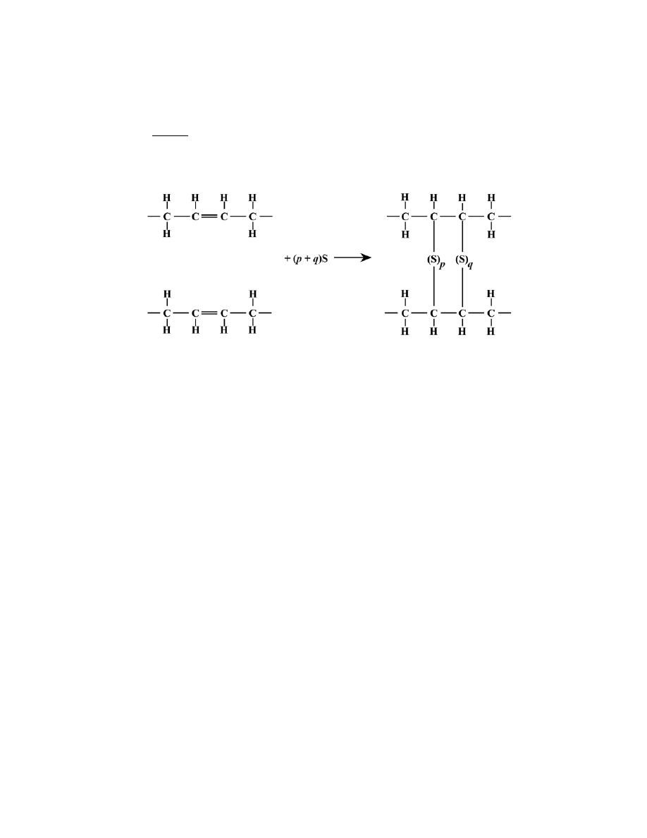
Excerpts from this work may be reproduced by instructors for distribution on a not-for-profit basis for testing or instructional purposes only to
students enrolled in courses for which the textbook has been adopted. Any other reproduction or translation of this work beyond that permitted
by Sections 107 or 108 of the 1976 United States Copyright Act without the permission of the copyright owner is unlawful.
15.29 Demonstrate, in a manner similar to Equation 15.4, how vulcanization may occur in a butadiene
rubber.
Solution
The reaction by which a butadiene rubber may become vulcanized is as follows:

Excerpts from this work may be reproduced by instructors for distribution on a not-for-profit basis for testing or instructional purposes only to
students enrolled in courses for which the textbook has been adopted. Any other reproduction or translation of this work beyond that permitted
by Sections 107 or 108 of the 1976 United States Copyright Act without the permission of the copyright owner is unlawful.
Crystallization
15.30 Determine values for the constants n and k (Equation 10.17) for the crystallization of polypropylene
(Figure 15.17) at 160°C.
Solution
In this problem we are asked to determine the values of the constants n and k (Equation 10.17) for the
crystallization of polypropylene at 160
°C (Figure 15.17). One way to solve this problem is to take two values of
percent recrystallization (which is just 100y, Equation 10.17) and their corresponding time values, then set up two
simultaneous equations, from which n and k may be determined. In order to expedite this process, we will rearrange
and do some algebraic manipulation of Equation 10.17. First of all, we rearrange as follows:
1
− y = exp − kt
n
( )
Now taking natural logarithms
ln (1
− y) = − kt
n
Or
− ln (1 − y) = kt
n
which may also be expressed as
ln
1
1
− y
= kt
n
Now taking natural logarithms again, leads to
ln ln
1
1
− y
= ln k + n ln t
which is the form of the equation that we will now use. From the 160
°C curve of Figure 15.17, let us arbitrarily
choose two percent crystallized values of 20% and 80% (i.e., y
1
= 0.20 and y
2
= 0.80). The corresponding time

Excerpts from this work may be reproduced by instructors for distribution on a not-for-profit basis for testing or instructional purposes only to
students enrolled in courses for which the textbook has been adopted. Any other reproduction or translation of this work beyond that permitted
by Sections 107 or 108 of the 1976 United States Copyright Act without the permission of the copyright owner is unlawful.
values are t
1
= 3400 min and t
2
= 6700 min (realizing that the time axis is scaled logarithmically). Thus, our two
simultaneous equations become
ln ln
1
1
− 0.20
= ln k + n ln (3400)
ln ln
1
1
− 0.80
= ln k + n ln (6700)
from which we obtain the values n = 2.91 and k = 1.182
× 10
-11
.

Excerpts from this work may be reproduced by instructors for distribution on a not-for-profit basis for testing or instructional purposes only to
students enrolled in courses for which the textbook has been adopted. Any other reproduction or translation of this work beyond that permitted
by Sections 107 or 108 of the 1976 United States Copyright Act without the permission of the copyright owner is unlawful.
Melting and Glass Transition Temperatures
15.31 Name the following polymer(s) that would be suitable for the fabrication of cups to contain hot
coffee: polyethylene, polypropylene, poly(vinyl chloride), PET polyester, and polycarbonate. Why?
Solution
This question asks us to name which, of several polymers, would be suitable for the fabrication of cups to
contain hot coffee. At its glass transition temperature, an amorphous polymer begins to soften. The maximum
temperature of hot coffee is probably slightly below 100
°C (212°F). Of the polymers listed, only polystyrene and
polycarbonate have glass transition temperatures of 100
°C or above (Table 15.2), and would be suitable for this
application.

Excerpts from this work may be reproduced by instructors for distribution on a not-for-profit basis for testing or instructional purposes only to
students enrolled in courses for which the textbook has been adopted. Any other reproduction or translation of this work beyond that permitted
by Sections 107 or 108 of the 1976 United States Copyright Act without the permission of the copyright owner is unlawful.
15.32 Of those polymers listed in Table 15.2, which polymer(s) would be best suited for use as ice cube
trays? Why?
Solution
In order for a polymer to be suited for use as an ice cube tray it must have a glass-transition temperature
below 0
°C. Of those polymers listed in Table 15.2 only low-density and high-density polyethylene, PTFE, and
polypropylene satisfy this criterion.
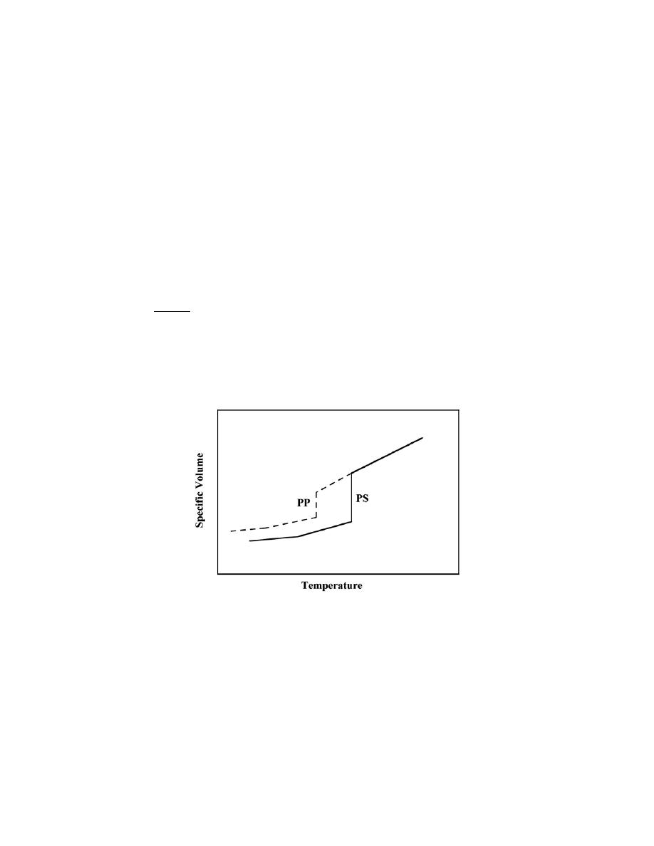
Excerpts from this work may be reproduced by instructors for distribution on a not-for-profit basis for testing or instructional purposes only to
students enrolled in courses for which the textbook has been adopted. Any other reproduction or translation of this work beyond that permitted
by Sections 107 or 108 of the 1976 United States Copyright Act without the permission of the copyright owner is unlawful.
Factors That Influence Melting and Glass Transition Temperatures
15.33 For each of the following pairs of polymers, plot and label schematic specific volume versus
temperature curves on the same graph [i.e., make separate plots for parts (a), (b), and (c)].
(a) Spherulitic polypropylene, of 25% crystallinity, and having a weight-average molecular weight of
75,000 g/mol; spherulitic polystyrene, of 25% crystallinity, and having a weight-average molecular weight of
100,000 g/mol
(b) Graft poly(styrene-butadiene) copolymer with 10% of available sites crosslinked; random poly(styrene-
butadiene) copolymer with 15% of available sites crosslinked
(c) Polyethylene having a density of 0.985 g/cm
3
and a degree of polymerization of 2500; polyethylene
having a density of 0.915 g/cm
3
and a degree of polymerization of 2000
Solution
(a) Shown below are the specific volume-versus-temperature curves for the polypropylene and polystyrene
materials. Since both polymers are 25% crystalline, they will exhibit behavior similar to curve B in Figure 15.18.
However, polystyrene will have higher melting and glass transition temperatures due to the bulkier side group in its
repeat unit structure, and since it has a higher weight-average molecular weight.
(b) Shown below are the specific volume-versus-temperature curves for the graft and random poly(styrene-
butadiene) copolymers. Since these materials are graft and random copolymers, both will be highly noncrystalline,
and, thus, will display the behavior similar to curve A in Figure 15.18. However, since the random has the greater
degree of crosslinking, it will also have the higher glass transition temperature.
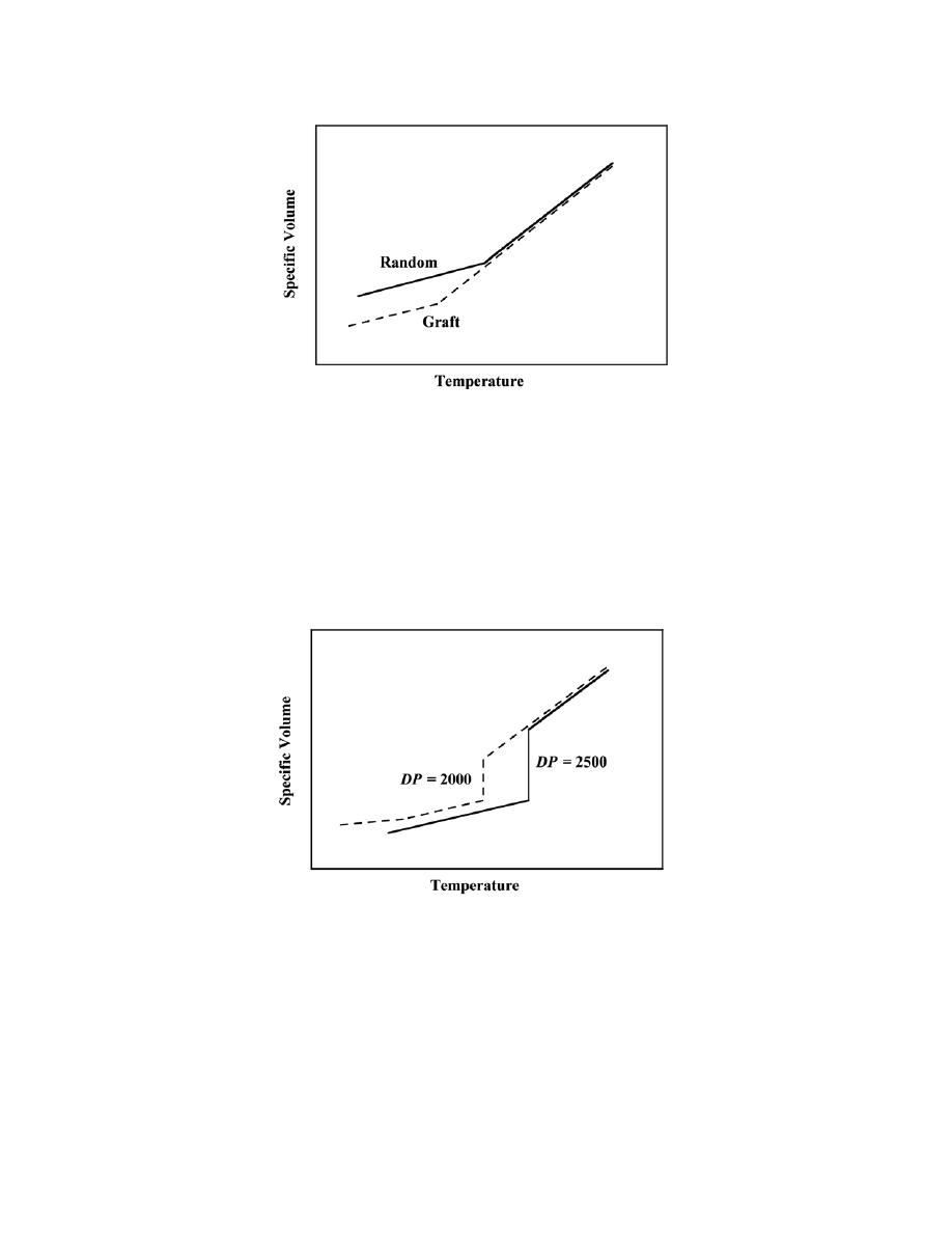
Excerpts from this work may be reproduced by instructors for distribution on a not-for-profit basis for testing or instructional purposes only to
students enrolled in courses for which the textbook has been adopted. Any other reproduction or translation of this work beyond that permitted
by Sections 107 or 108 of the 1976 United States Copyright Act without the permission of the copyright owner is unlawful.
(c) Shown below are the specific volume-versus-temperature curves for the two polyethylene materials.
The polyethylene having a density of 0.985 g/cm
3
will be highly crystalline, and, thus, will exhibit a behavior
similar to curve C in Figure 15.18. On the other hand, the other material, of lower density will have some branching
and also be semicrystalline; thus, its behavior will be similar to curve B of Figure 15.18. In addition, the melting
temperature of the higher density material will be greater since it has less branching and a higher degree of
polymerization.

Excerpts from this work may be reproduced by instructors for distribution on a not-for-profit basis for testing or instructional purposes only to
students enrolled in courses for which the textbook has been adopted. Any other reproduction or translation of this work beyond that permitted
by Sections 107 or 108 of the 1976 United States Copyright Act without the permission of the copyright owner is unlawful.
15.34 For each of the following pairs of polymers, do the following: (1) state whether or not it is possible
to determine whether one polymer has a higher melting temperature than the other; (2) if it is possible, note which
has the higher melting temperature and then cite reason(s) for your choice; and (3) if it is not possible to decide,
then state why.
(a) Isotactic polystyrene that has a density of 1.12 g/cm
3
and a weight-average molecular weight of
150,000 g/mol; syndiotactic polystyrene that has a density of 1.10 g/cm
3
and a weight-average molecular weight of
125,000 g/mol
(b) Linear polyethylene that has a degree of polymerization of 5,000; linear and isotactic polypropylene
that has a degree of polymerization of 6,500
(c) Branched and isotactic polystyrene that has a degree of polymerization of 4,000; linear and isotactic
polypropylene that has a degree of polymerization of 7,500
Solution
(a) Yes, it is possible to determine which of the two polystyrenes has the higher T
m
. The isotactic
polystyrene will have the higher melting temperature because it has a higher density (i.e., less branching) and also
the greater weight-average molecular weight.
(b) Yes, it is possible to determine which polymer has the higher melting temperature. The polypropylene
will have the higher T
m
because it has a bulky phenyl side group in its repeat unit structure, which is absent in the
polyethylene. Furthermore, the polypropylene has a higher degree of polymerization.
(c) No, it is not possible to determine which of the two polymers has the higher melting temperature. The
polystyrene has a bulkier side group than the polypropylene; on the basis of this effect alone, the polystyrene
should have the greater T
m
. However, the polystyrene has more branching and a lower degree of polymerization;
both of these factors lead to a lowering of the melting temperature.
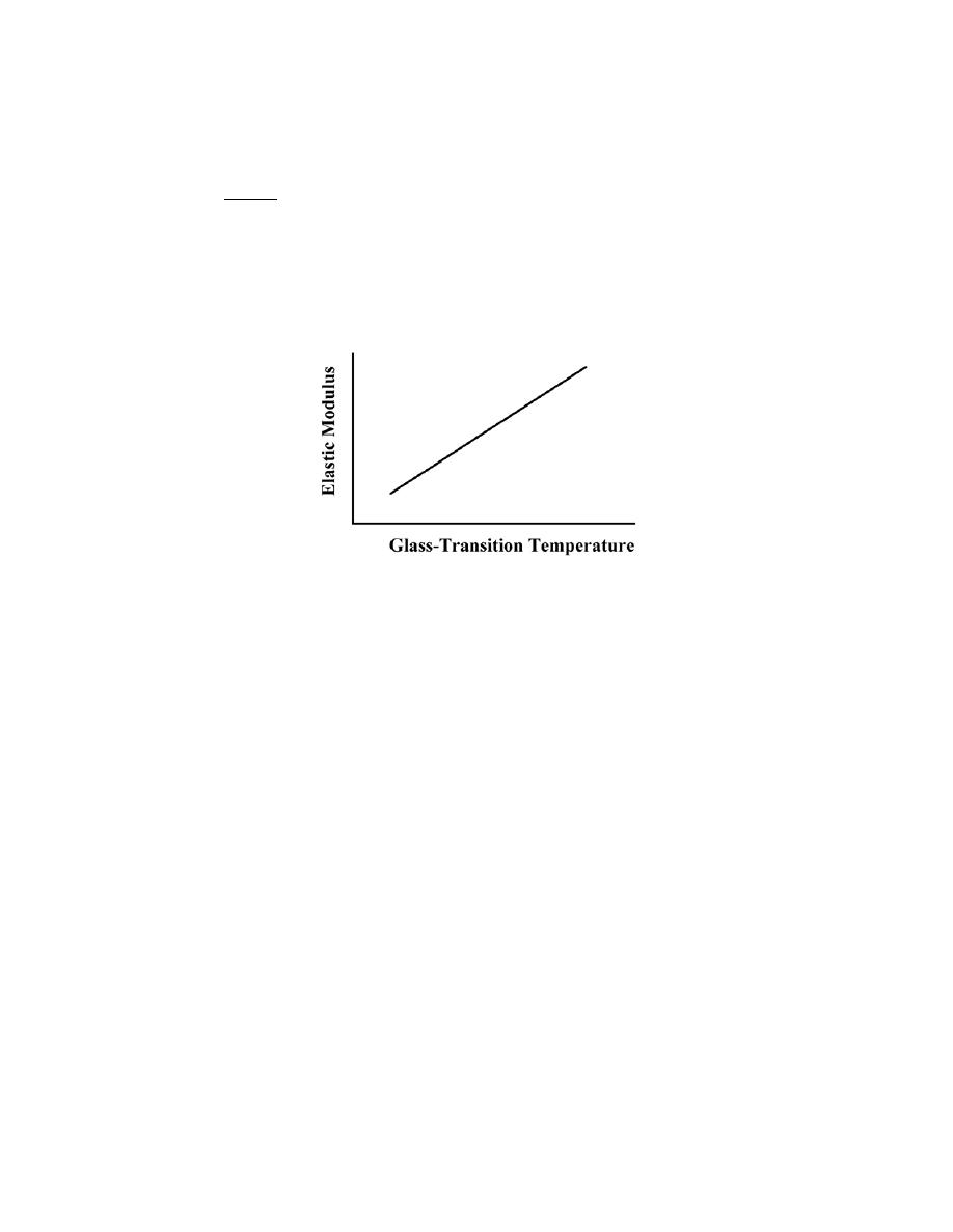
Excerpts from this work may be reproduced by instructors for distribution on a not-for-profit basis for testing or instructional purposes only to
students enrolled in courses for which the textbook has been adopted. Any other reproduction or translation of this work beyond that permitted
by Sections 107 or 108 of the 1976 United States Copyright Act without the permission of the copyright owner is unlawful.
15.35 Make a schematic plot showing how the modulus of elasticity of an amorphous polymer depends on
the glass transition temperature. Assume that molecular weight is held constant.
Solution
For an amorphous polymer, the elastic modulus may be enhanced by increasing the number of crosslinks
(while maintaining the molecular weight constant); this will also enhance the glass transition temperature. Thus,
the modulus-glass transition temperature behavior would appear as

Excerpts from this work may be reproduced by instructors for distribution on a not-for-profit basis for testing or instructional purposes only to
students enrolled in courses for which the textbook has been adopted. Any other reproduction or translation of this work beyond that permitted
by Sections 107 or 108 of the 1976 United States Copyright Act without the permission of the copyright owner is unlawful.
Elastomers
Fibers
Miscellaneous Applications
15.36 Briefly explain the difference in molecular chemistry between silicone polymers and other polymeric
materials.
Solution
The backbone chain of most polymers consists of carbon atoms that are linked together. For the silicone
polymers, this backbone chain is composed of silicon and oxygen atoms that alternate positions.

Excerpts from this work may be reproduced by instructors for distribution on a not-for-profit basis for testing or instructional purposes only to
students enrolled in courses for which the textbook has been adopted. Any other reproduction or translation of this work beyond that permitted
by Sections 107 or 108 of the 1976 United States Copyright Act without the permission of the copyright owner is unlawful.
15.37 List two important characteristics for polymers that are to be used in fiber applications.
Solution
Two important characteristics for polymers that are to be used in fiber applications are: (1) they must have
high molecular weights, and (2) they must have chain configurations/structures that will allow for high degrees of
crystallinity.

Excerpts from this work may be reproduced by instructors for distribution on a not-for-profit basis for testing or instructional purposes only to
students enrolled in courses for which the textbook has been adopted. Any other reproduction or translation of this work beyond that permitted
by Sections 107 or 108 of the 1976 United States Copyright Act without the permission of the copyright owner is unlawful.
15.38 Cite five important characteristics for polymers that are to be used in thin-film applications.
Solution
Five important characteristics for polymers that are to be used in thin-film applications are: (1) low
density; (2) high flexibility; (3) high tensile and tear strengths; (4) resistance to moisture/chemical attack; and (5)
low gas permeability.

Excerpts from this work may be reproduced by instructors for distribution on a not-for-profit basis for testing or instructional purposes only to
students enrolled in courses for which the textbook has been adopted. Any other reproduction or translation of this work beyond that permitted
by Sections 107 or 108 of the 1976 United States Copyright Act without the permission of the copyright owner is unlawful.
Polymerization
15.39 Cite the primary differences between addition and condensation polymerization techniques.
Solution
For addition polymerization, the reactant species have the same chemical composition as the monomer
species in the molecular chain. This is not the case for condensation polymerization, wherein there is a chemical
reaction between two or more monomer species, producing the repeating unit. There is often a low molecular
weight by-product for condensation polymerization; such is not found for addition polymerization.

Excerpts from this work may be reproduced by instructors for distribution on a not-for-profit basis for testing or instructional purposes only to
students enrolled in courses for which the textbook has been adopted. Any other reproduction or translation of this work beyond that permitted
by Sections 107 or 108 of the 1976 United States Copyright Act without the permission of the copyright owner is unlawful.
15.40 (a) How much ethylene glycol must be added to 47.3 kg of terephthalic acid to produce a linear
chain structure of poly(ethylene terephthalate) according to Equation 15.9?
(b) What is the mass of the resulting polymer?
Solution
(a) This problem asks that we determine how much ethylene glycol must be added to 47.3 kg of
terephthalic acid to produce a linear chain structure of poly(ethylene terephthalate) according to Equation 15.9.
Since the chemical formulas are provided in this equation we may calculate the molecular weights of each of these
materials as follows:
MW(ethylene glycol) = 2( A
C
) + 6( A
H
) + 2( A
O
)
= 2 (12.01 g/mol) + 6 (1.008 g/mol) + 2 (16.00 g/mol) = 62.07 g/mol
MW(terephthalic acid) = 8( A
C
) + 6( A
H
) + 4( A
O
)
= 8 (12.01 g/mol) + 6 (1.008 g/mol) + 4 (16.00 g/mol) = 166.13 g/mol
The 47.3 kg mass of terephthalic acid equals 47,300 g or
47, 300 g
166.13 g / mol
= 284.72 mol. Since, according to
Equation 15.9, each mole of terephthalic acid used requires one mole of ethylene glycol, which is equivalent to
(284.72 mol)(62.07 g/mol) = 17,673 g = 17.673 kg.
(b) Now we are asked for the mass of the resulting polymer. Inasmuch as one mole of water is given off
for every repeat unit produced, this corresponds to 284.72 moles or (284.72 mol)(18.02 g/mol) = 5130 g or 5.130 kg
since the molecular weight of water is 18.02 g/mol. The mass of poly(ethylene terephthalate) is just the sum of the
masses of the two reactant materials [as computed in part (a)] minus the mass of water released, or
mass [poly(ethylene terephthalate)] = 47.300 kg + 17.673 kg
− 5.130 kg = 59.843 kg
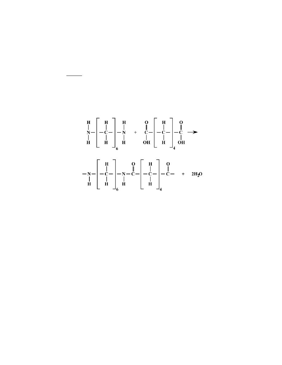
Excerpts from this work may be reproduced by instructors for distribution on a not-for-profit basis for testing or instructional purposes only to
students enrolled in courses for which the textbook has been adopted. Any other reproduction or translation of this work beyond that permitted
by Sections 107 or 108 of the 1976 United States Copyright Act without the permission of the copyright owner is unlawful.
15.41 Nylon 6,6 may be formed by means of a condensation polymerization reaction in which
hexamethylene diamine [NH
2
—(CH
2
)
6
—NH
2
] and adipic acid react with one another with the formation of water
as a byproduct. What masses of hexamethylene diamine and adipic acid are necessary to yield 37.5 kg of completely
linear nylon 6,6? (Note: the chemical equation for this reaction is the answer to Concept Check 15.12.)
Solution
This problem asks for us to calculate the masses of hexamethylene diamine and adipic acid necessary to
yield 37.5 kg of completely linear nylon 6,6. The chemical equation for this reaction is the answer to Concept
Check 15.12, which is as follows:
From this equation we may calculate the molecular weights of these molecules.
MW(adipic) = 6( A
C
) + 10( A
H
) + 4( A
O
)
= 6 (12.01 g/mol) + 10 (1.008 g/mol) + 4 (16.00 g/mol) = 146.14 g/mol
MW(hexamethylene) = 6( A
C
) + 16( A
H
) + 2( A
N
)
= 6 (12.01 g/mol) + 16 (1.008 g/mol) + 2 (14.01 g/mol) = 116.21 g/mol
MW(nylon) = 12( A
C
) + 22( A
H
) + 2( A
N
) + 2( A
O
)

Excerpts from this work may be reproduced by instructors for distribution on a not-for-profit basis for testing or instructional purposes only to
students enrolled in courses for which the textbook has been adopted. Any other reproduction or translation of this work beyond that permitted
by Sections 107 or 108 of the 1976 United States Copyright Act without the permission of the copyright owner is unlawful.
= 12 (12.01 g/mol) + 22 (1.008 g/mol) + 2 (14.01 g/mol) + 2 (16.00 g/mol)
= 226.32 g/mol
The mass of 37.5 kg of nylon 6,6 equals 37,500 g or
m(nylon) =
37, 500 g
226.32 g / mol
= 165.7 mol
Since, according to the chemical equation given above, each mole of nylon 6,6 that is produced requires one mole
each of adipic acid and hexamethylene diamine, with two moles of water as the by-product. The masses
corresponding to 165.7 moles of adipic acid and hexamethylene diamine are as follows:
m(adipic) = (165.7 mol)(146.14 g/mol) = 24, 215 g = 24.215 kg
m(hexamethylene) = (165.7 mol)(116.21 g/mol) = 19, 256 g = 19.256 kg

Excerpts from this work may be reproduced by instructors for distribution on a not-for-profit basis for testing or instructional purposes only to
students enrolled in courses for which the textbook has been adopted. Any other reproduction or translation of this work beyond that permitted
by Sections 107 or 108 of the 1976 United States Copyright Act without the permission of the copyright owner is unlawful.
Polymer Additives
15.42 What is the distinction between dye and pigment colorants?
Solution
The distinction between dye and pigment colorants is that a dye dissolves within and becomes a part of the
polymer structure, whereas a pigment does not dissolve, but remains as a separate phase.

Excerpts from this work may be reproduced by instructors for distribution on a not-for-profit basis for testing or instructional purposes only to
students enrolled in courses for which the textbook has been adopted. Any other reproduction or translation of this work beyond that permitted
by Sections 107 or 108 of the 1976 United States Copyright Act without the permission of the copyright owner is unlawful.
Forming Techniques for Plastics
15.43 Cite four factors that determine what fabrication technique is used to form polymeric materials.
Solution
Four factors that determine what fabrication technique is used to form polymeric materials are: (1) whether
the polymer is thermoplastic or thermosetting; (2) if thermoplastic, the softening temperature; (3) atmospheric
stability; and (4) the geometry and size of the finished product.

Excerpts from this work may be reproduced by instructors for distribution on a not-for-profit basis for testing or instructional purposes only to
students enrolled in courses for which the textbook has been adopted. Any other reproduction or translation of this work beyond that permitted
by Sections 107 or 108 of the 1976 United States Copyright Act without the permission of the copyright owner is unlawful.
15.44 Contrast compression, injection, and transfer molding techniques that are used to form plastic
materials.
Solution
This question requests that we compare polymer molding techniques. For compression molding, both heat
and pressure are applied after the polymer and necessary additives are situated between the mold members. For
transfer molding, the solid materials (normally thermosetting in nature) are first melted in the transfer chamber prior
to being forced into the die. And, for injection molding (normally used for thermoplastic materials), the raw
materials are impelled by a ram through a heating chamber, and finally into the die cavity.

Excerpts from this work may be reproduced by instructors for distribution on a not-for-profit basis for testing or instructional purposes only to
students enrolled in courses for which the textbook has been adopted. Any other reproduction or translation of this work beyond that permitted
by Sections 107 or 108 of the 1976 United States Copyright Act without the permission of the copyright owner is unlawful.
Fabrication of Fibers and Films
15.45 Why must fiber materials that are melt spun and then drawn be thermoplastic? Cite two reasons.
Solution
Fiber materials that are melt spun must be thermoplastic because: (1) In order to be melt spun, they must
be capable of forming a viscous liquid when heated, which is not possible for thermosets. (2) During drawing,
mechanical elongation must be possible; inasmuch as thermosetting materials are, in general, hard and relatively
brittle, they are not easily elongated.

Excerpts from this work may be reproduced by instructors for distribution on a not-for-profit basis for testing or instructional purposes only to
students enrolled in courses for which the textbook has been adopted. Any other reproduction or translation of this work beyond that permitted
by Sections 107 or 108 of the 1976 United States Copyright Act without the permission of the copyright owner is unlawful.
15.46 Which of the following polyethylene thin films would have the better mechanical characteristics: (1)
formed by blowing, or (2) formed by extrusion and then rolled? Why?
Solution
Of the two polymers cited, the one that was formed by extrusion and then rolled would have the higher
strength. Both blown and extruded materials would have roughly comparable strengths; however the rolling
operation would further serve to enhance the strength of the extruded material.

Excerpts from this work may be reproduced by instructors for distribution on a not-for-profit basis for testing or instructional purposes only to
students enrolled in courses for which the textbook has been adopted. Any other reproduction or translation of this work beyond that permitted
by Sections 107 or 108 of the 1976 United States Copyright Act without the permission of the copyright owner is unlawful.
DESIGN QUESTIONS
15.D1 (a) List several advantages and disadvantages of using transparent polymeric materials for eyeglass
lenses.
(b) Cite four properties (in addition to being transparent) that are important for this application.
(c) Note three polymers that may be candidates for eyeglass lenses, and then tabulate values of the
properties noted in part (b) for these three materials.
Solution
(a) Several advantages of using transparent polymeric materials for eyeglass lenses are: they have
relatively low densities, and, therefore, are light in weight; they are relatively easy to grind to have the desired
contours; they are less likely to shatter than are glass lenses; wraparound lenses for protection during sports
activities are possible; and they filter out more ultraviolet radiation than do glass lenses.
The principal disadvantage of these types of lenses is that some are relatively soft and are easily scratched
(although antiscratch coatings may be applied). Plastic lenses are not as mechanically stable as glass, and, therefore,
are not as precise optically.
(b) Some of the properties that are important for polymer lens materials are: they should be relatively hard
in order to resist scratching; they must be impact resistant; they should be shatter resistant; they must have a
relatively high index of refraction such that thin lenses may be ground for very nearsighted people; and they should
absorb significant proportions of all types of ultraviolet radiation, which radiation can do damage to the eye tissues.
(c) Of those polymers discussed in this chapter and Chapter 14, likely lens candidates are polystyrene,
poly(methyl methacrylate), and polycarbonate; these three materials are not easily crystallized, and, therefore, are
normally transparent. Upon consultation of their fracture toughnesses (Table B.5 in Appendix B), polycarbonate is
the most superior of the three.
Commercially, the two plastic lens materials of choice are polycarbonate and allyl diglycol carbonate
(having the trade name CR-39). Polycarbonate is very impact resistant, but not as hard as CR-39. Furthermore, PC
comes in both normal and high refractive-index grades.

Excerpts from this work may be reproduced by instructors for distribution on a not-for-profit basis for testing or instructional purposes only to
students enrolled in courses for which the textbook has been adopted. Any other reproduction or translation of this work beyond that permitted
by Sections 107 or 108 of the 1976 United States Copyright Act without the permission of the copyright owner is unlawful.
15.D2 Write an essay on polymeric materials that are used in the packaging of food products and drinks.
Include a list of the general requisite characteristics of materials that are used for these applications. Now cite a
specific material that is utilized for each of three different container types and the rationale for each choice.
Solution
There are three primary requirements for polymeric materials that are utilized in the packaging of food
products and drinks; these are: (1) sufficient strength, to include tensile, tear, and impact strengths; (2) barrier
protection--that is, being resistant to permeation by oxygen, water vapor, and carbon dioxide; and (3) being
nonreactive with the food/drink contents--such reactions can compromise the integrity of the packaging material, or
they can produce toxic by-products.
With regard to strength, poly(ethylene terephthalate) (PET or PETE) and oriented polypropylene (OPP)
have high tensile strengths, linear low-density polyethylene (LLDPE) and low-density polyethylene (LDPE) have
high tear strengths, while those polymers having the best impact strengths are PET and poly(vinyl chloride) (PVC).
Relative to barrier characteristics, ethylene vinyl alcohol (EVOH) and poly(vinylidene chloride) (PVDC)
copolymers are relatively impermeable to oxygen and carbon dioxide, whereas high-density polyethylene (HDPE),
PVDC, polypropylene, and LDPE are impervious to water vapor.
Most common polymers are relatively nonreactive with food products, and are considered safe; exceptions
are acrylonitrile and plasticizers used in PVC materials.
The aesthetics of packaging polymers are also important in the marketing of food and drink products.
Some will be colored, many are adorned with printing, others need to be transparent and clear, and many need to be
resistant to scuffing.
On the basis of the preceding discussion, examples of polymers that are used for specific applications are
as follows:
PET(E) for soda pop containers;
PVC for beer containers;
LDPE and HDPE films for packaging bread and bakery products.

Excerpts from this work may be reproduced by instructors for distribution on a not-for-profit basis for testing or instructional purposes only to
students enrolled in courses for which the textbook has been adopted. Any other reproduction or translation of this work beyond that permitted
by Sections 107 or 108 of the 1976 United States Copyright Act without the permission of the copyright owner is unlawful.
15.D3 Write an essay on the replacement of metallic automobile components by polymers and composite
materials. Address the following issues: (1) Which automotive components (e.g., crankshaft) now use polymers
and/or composites? (2) Specifically what materials (e.g., high-density polyethylene) are now being used? (3) What
are the reasons for these replacements?
Solution
The primary reasons that the automotive industry has replaced metallic automobile components with
polymer and composite materials are: polymers/composites (1) have lower densities, and afford higher fuel
efficiencies; (2) may be produced at lower costs but with comparable mechanical characteristics; (3) are in many
environments more corrosion resistant; (4) reduce noise, and (5) are thermally insulating and thus reduce the
transference of heat.
These replacements are many and varied. Several are as follows:
Bumper fascia are molded from an elastomer-modified polypropylene.
Overhead consoles are made of poly(phenylene oxide) and recycled polycarbonate.
Rocker arm covers are injection molded of a glass- and mineral-reinforced nylon 6,6 composite.
Torque converter reactors, water outlets, pulleys, and brake pistons, are made from phenolic thermoset
composites that are reinforced with glass fibers.
Air intake manifolds are made of a glass-reinforced nylon 6,6.
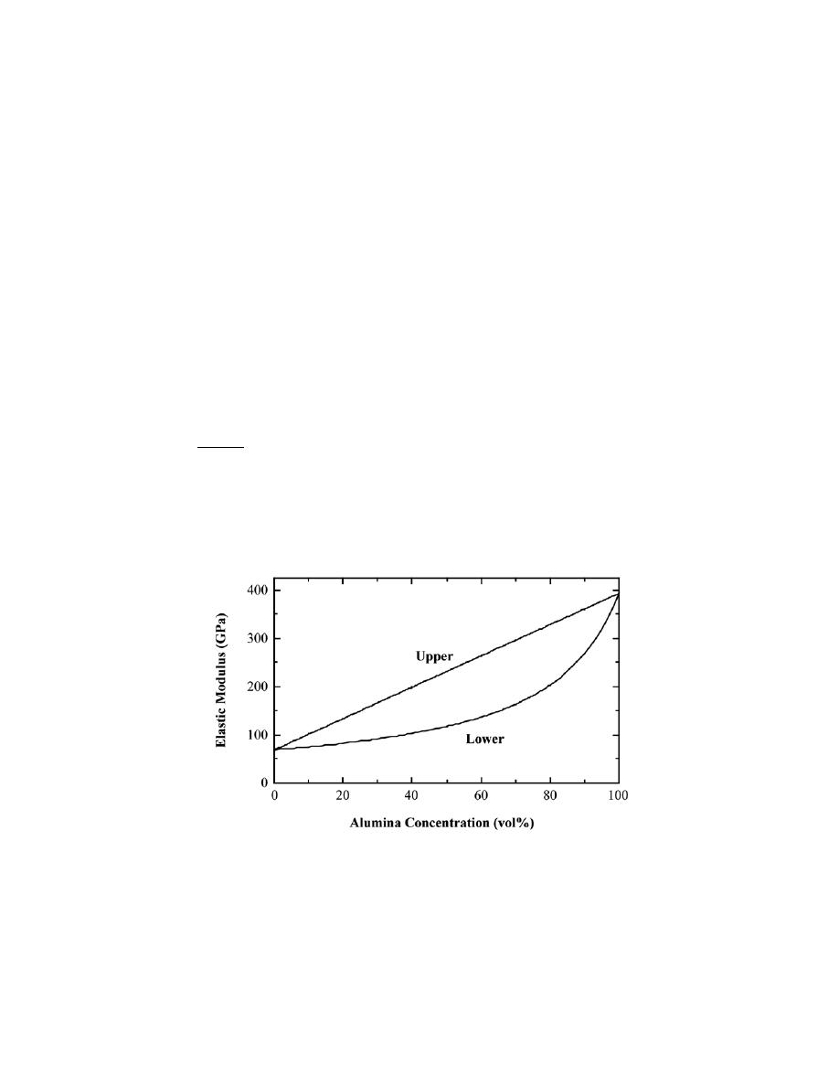
Excerpts from this work may be reproduced by instructors for distribution on a not-for-profit basis for testing or instructional purposes only to
students enrolled in courses for which the textbook has been adopted. Any other reproduction or translation of this work beyond that permitted
by Sections 107 or 108 of the 1976 United States Copyright Act without the permission of the copyright owner is unlawful.
CHAPTER 16
COMPOSITES
PROBLEM SOLUTIONS
Large-Particle Composites
16.1 The mechanical properties of aluminum may be improved by incorporating fine particles of
aluminum oxide (Al
2
O
3
). Given that the moduli of elasticity of these materials are, respectively, 69 GPa (10
× 10
6
psi) and 393 GPa (57
× 10
6
psi), plot modulus of elasticity versus the volume percent of Al
2
O
3
in Al from 0 to 100
vol%, using both upper- and lower-bound expressions.
Solution
The elastic modulus versus the volume percent of Al
2
O
3
is shown below, on which is included both upper
and lower bound curves; these curves were generated using Equations 16.1 and 16.2, respectively, and using the
moduli of elasticity for aluminum and Al
2
O
3
that were given in the problem statement.

Excerpts from this work may be reproduced by instructors for distribution on a not-for-profit basis for testing or instructional purposes only to
students enrolled in courses for which the textbook has been adopted. Any other reproduction or translation of this work beyond that permitted
by Sections 107 or 108 of the 1976 United States Copyright Act without the permission of the copyright owner is unlawful.
16.2 Estimate the maximum and minimum thermal conductivity values for a cermet that contains 85 vol%
titanium carbide (TiC) particles in a cobalt matrix. Assume thermal conductivities of 27 and 69 W/m-K for TiC and
Co, respectively.
Solution
This problem asks for the maximum and minimum thermal conductivity values for a TiC-Co cermet.
Using a modified form of Equation 16.1 the maximum thermal conductivity k
max
is calculated as
k
max
= k
m
V
m
+ k
p
V
p
= k
Co
V
Co
+ k
TiC
V
TiC
= (69 W/m - K)(0.15) + (27 W/m - K)(0.85) = 33.3 W/m - K
Using a modified form of Equation 16.2, the minimum thermal conductivity k
min
will be
k
min
=
k
Co
k
TiC
V
Co
k
TiC
+ V
TiC
k
Co
=
(69 W/m - K)(27 W/m - K)
(0.15)(27 W/m - K)
+ (0.85)(69 W/m - K)
= 29.7 W/m-K

Excerpts from this work may be reproduced by instructors for distribution on a not-for-profit basis for testing or instructional purposes only to
students enrolled in courses for which the textbook has been adopted. Any other reproduction or translation of this work beyond that permitted
by Sections 107 or 108 of the 1976 United States Copyright Act without the permission of the copyright owner is unlawful.
16.3 A large-particle composite consisting of tungsten particles within a copper matrix is to be prepared.
If the volume fractions of tungsten and copper are 0.60 and 0.40, respectively, estimate the upper limit for the
specific stiffness of this composite given the data that follow.
Specific Gravity
Modulus of Elasticity
(GPa)
Copper
8.9
110
Tungsten
19.3
407
Solution
Given the elastic moduli and specific gravities for copper and tungsten we are asked to estimate the upper
limit for specific stiffness when the volume fractions of tungsten and copper are 0.60 and 0.40, respectively. There
are two approaches that may be applied to solve this problem. The first is to estimate both the upper limits of elastic
modulus [E
c
(u)] and specific gravity (
ρ
c
) for the composite, using expressions of the form of Equation 16.1, and
then take their ratio. Using this approach
E
c
(u) = E
Cu
V
Cu
+ E
W
V
W
= (110 GPa)(0.40) + (407 GPa)(0.60)
= 288 GPa
And
ρ
c
=
ρ
Cu
V
Cu
+
ρ
W
V
W
= (8.9)(0.40) + (19.3)(0.60) = 15.14
Therefore
Specific Stiffness =
E
c
(u)
ρ
c
=
288 GPa
15.14
= 19.0 GPa
With the alternate approach, the specific stiffness is calculated, again employing a modification of
Equation 16.1, but using the specific stiffness-volume fraction product for both metals, as follows:

Excerpts from this work may be reproduced by instructors for distribution on a not-for-profit basis for testing or instructional purposes only to
students enrolled in courses for which the textbook has been adopted. Any other reproduction or translation of this work beyond that permitted
by Sections 107 or 108 of the 1976 United States Copyright Act without the permission of the copyright owner is unlawful.
Specific Stiffness =
E
Cu
ρ
Cu
V
Cu
+
E
W
ρ
W
V
W
=
110 GPa
8.9
(0.40) +
407 GPa
19.3
(0.60) = 17.6 GPa

Excerpts from this work may be reproduced by instructors for distribution on a not-for-profit basis for testing or instructional purposes only to
students enrolled in courses for which the textbook has been adopted. Any other reproduction or translation of this work beyond that permitted
by Sections 107 or 108 of the 1976 United States Copyright Act without the permission of the copyright owner is unlawful.
16.4 (a) What is the distinction between cement and concrete?
(b) Cite three important limitations that restrict the use of concrete as a structural material.
(c) Briefly explain three techniques that are utilized to strengthen concrete by reinforcement.
Solution
(a) Concrete consists of an aggregate of particles that are bonded together by a cement.
(b) Three limitations of concrete are: (1) it is a relatively weak and brittle material; (2) it experiences
relatively large thermal expansions (contractions) with changes in temperature; and (3) it may crack when exposed
to freeze-thaw cycles.
(c) Three reinforcement strengthening techniques are: (1) reinforcement with steel wires, rods, etc.; (2)
reinforcement with fine fibers of a high modulus material; and (3) introduction of residual compressive stresses by
prestressing or posttensioning.

Excerpts from this work may be reproduced by instructors for distribution on a not-for-profit basis for testing or instructional purposes only to
students enrolled in courses for which the textbook has been adopted. Any other reproduction or translation of this work beyond that permitted
by Sections 107 or 108 of the 1976 United States Copyright Act without the permission of the copyright owner is unlawful.
Dispersion-Strengthened Composites
16.5 Cite one similarity and two differences between precipitation hardening and dispersion
strengthening.
Solution
The similarity between precipitation hardening and dispersion strengthening is the strengthening
mechanism--i.e., the precipitates/particles effectively hinder dislocation motion.
The two differences are: (1) the hardening/strengthening effect is not retained at elevated temperatures for
precipitation hardening--however, it is retained for dispersion strengthening; and (2) the strength is developed by a
heat treatment for precipitation hardening--such is not the case for dispersion strengthening.

Excerpts from this work may be reproduced by instructors for distribution on a not-for-profit basis for testing or instructional purposes only to
students enrolled in courses for which the textbook has been adopted. Any other reproduction or translation of this work beyond that permitted
by Sections 107 or 108 of the 1976 United States Copyright Act without the permission of the copyright owner is unlawful.
Influence of Fiber Length
16.6 For some glass fiber-epoxy matrix combination, the critical fiber length-fiber diameter ratio is 50.
Using the data in Table 16.4, determine the fiber-matrix bond strength.
Solution
This problem asks that, for a glass fiber-epoxy matrix combination, to determine the fiber-matrix bond
strength if the critical fiber length-fiber diameter ratio is 50. Thus, we are to solve for
τ
c
in Equation 16.3. Since
we are given that
σ
f
∗
= 3.45 GPa from Table 16.4, and that
l
c
d
= 50, then
τ
c
=
σ
f
∗
d
2 l
c
=
(
3.45
× 10
3
MPa
)
1
2
1
50
= 34.5 MPa
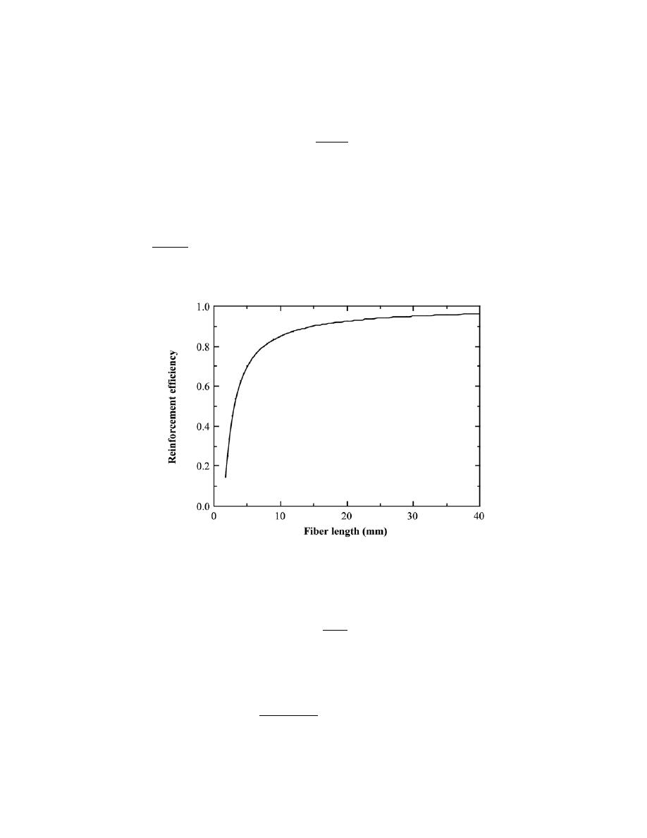
Excerpts from this work may be reproduced by instructors for distribution on a not-for-profit basis for testing or instructional purposes only to
students enrolled in courses for which the textbook has been adopted. Any other reproduction or translation of this work beyond that permitted
by Sections 107 or 108 of the 1976 United States Copyright Act without the permission of the copyright owner is unlawful.
16.7 (a) For a fiber-
reinforced composite, the efficiency of reinforcement η is dependent on fiber length l
according to
η =
l
− 2x
l
where x represents the length of the fiber at each end that does not contribute to the load transfer. Make a plot of η
versus l to l = 40 mm (1.6 in.) assuming that x = 0.75 mm (0.03 in.).
(b) What length is required for a 0.80 efficiency of reinforcement?
Solution
(a) The plot of reinforcement efficiency versus fiber length is given below.
(b) This portion of the problem asks for the length required for a 0.80 efficiency of reinforcement.
Solving for l from the given expression
l =
2x
1
− η
Or, when x = 0.75 mm (0.03 in.) and
η = 0.80, then
l =
(2)(0.75 mm)
1
− 0.80
= 7.5 mm (0.30 in.)

Excerpts from this work may be reproduced by instructors for distribution on a not-for-profit basis for testing or instructional purposes only to
students enrolled in courses for which the textbook has been adopted. Any other reproduction or translation of this work beyond that permitted
by Sections 107 or 108 of the 1976 United States Copyright Act without the permission of the copyright owner is unlawful.
Influence of Fiber Orientation and Concentration
16.8 A continuous and aligned fiber-reinforced composite is to be produced consisting of 30 vol% aramid
fibers and 70 vol% of a polycarbonate matrix; mechanical characteristics of these two materials are as follows:
Modulus of Elasticity
[GPa (psi)]
Tensile Strength [MPa
(psi)]
Aramid fiber
131 (19 × 10
6
)
3600 (520,000)
Polycarbonate
2.4 (3.5 × 10
5
)
65 (9425)
Also, the stress on the polycarbonate matrix when the aramid fibers fail is 45 MPa (6500 psi).
For this composite, compute
(a) the longitudinal tensile strength, and
(b) the longitudinal modulus of elasticity
Solution
This problem calls for us to compute the longitudinal tensile strength and elastic modulus of an aramid
fiber-reinforced polycarbonate composite.
(a) The longitudinal tensile strength is determined using Equation 16.17 as
σ
cl
∗
=
σ
m
'
(
1
− V
f
)
+
σ
f
∗
V
f
= (45 MPa)(0.70) + (3600)(0.30)
= 1100 MPa (160,000 psi)
(b) The longitudinal elastic modulus is computed using Equation 16.10a as
E
cl
= E
m
V
m
+ E
f
V
f
= (2.4 GPa)(0.70) + (131 GPa)(0.30)
= 41 GPa (5.95
× 10
6
psi)

Excerpts from this work may be reproduced by instructors for distribution on a not-for-profit basis for testing or instructional purposes only to
students enrolled in courses for which the textbook has been adopted. Any other reproduction or translation of this work beyond that permitted
by Sections 107 or 108 of the 1976 United States Copyright Act without the permission of the copyright owner is unlawful.
16.9 Is it possible to produce a continuous and oriented aramid fiber-epoxy matrix composite having
longitudinal and transverse moduli of elasticity of 57.1 GPa (8.28
× 10
6
psi) and 4.12 GPa (6
× 10
5
psi),
respectively? Why or why not? Assume that the modulus of elasticity of the epoxy is 2.4 GPa (3.50
× 10
5
psi).
Solution
This problem asks for us to determine if it is possible to produce a continuous and oriented aramid fiber-
epoxy matrix composite having longitudinal and transverse moduli of elasticity of 57.1 GPa and 4.12 GPa,
respectively, given that the modulus of elasticity for the epoxy is 2.4 GPa. Also, from Table 16.4 the value of E for
aramid fibers is 131 GPa. The approach to solving this problem is to calculate values of V
f
for both longitudinal and
transverse cases using the data and Equations 16.10b and 16.16; if the two V
f
values are the same then this
composite is possible.
For the longitudinal modulus E
cl
(using Equation 16.10b),
E
cl
= E
m
(
1
− V
fl
)
+ E
f
V
fl
57.1 GPa = (2.4 GPa)
(
1
− V
fl
)
+ (131 GPa)V
fl
Solving this expression for V
fl
(i.e., the volume fraction of fibers for the longitudinal case) yields V
fl
= 0.425.
Now, repeating this procedure for the transverse modulus E
ct
(using Equation 16.16)
E
ct
=
E
m
E
f
(
1
− V
ft
)
E
f
+ V
ft
E
m
4.12 GPa =
(2.4 GPa)(131 GPa)
(
1
− V
ft
)
(131 GPa)
+ V
ft
(2.4 GPa)
Solving this expression for V
ft
(i.e., the volume fraction of fibers for the transverse case), leads to V
ft
= 0.425.
Thus, since V
fl
and V
ft
are equal, the proposed composite is possible.

Excerpts from this work may be reproduced by instructors for distribution on a not-for-profit basis for testing or instructional purposes only to
students enrolled in courses for which the textbook has been adopted. Any other reproduction or translation of this work beyond that permitted
by Sections 107 or 108 of the 1976 United States Copyright Act without the permission of the copyright owner is unlawful.
16.10 For a continuous and oriented fiber-reinforced composite, the moduli of elasticity in the
longitudinal and transverse directions are 19.7 and 3.66 GPa (2.8
× 10
6
and 5.3
× 10
5
psi), respectively. If the
volume fraction of fibers is 0.25, determine the moduli of elasticity of fiber and matrix phases.
Solution
This problem asks for us to compute the elastic moduli of fiber and matrix phases for a continuous and
oriented fiber-reinforced composite. We can write expressions for the longitudinal and transverse elastic moduli
using Equations 16.10b and 16.16, as
E
cl
= E
m
(
1
− V
f
)
+ E
f
V
f
19.7 GPa = E
m
(1
− 0.25) + E
f
(0.25)
And
E
ct
=
E
m
E
f
(
1
− V
f
)
E
f
+V
f
E
m
3.66 GPa =
E
m
E
f
(1
− 0.25)E
f
+ 0.25E
m
Solving these two expressions simultaneously for E
m
and E
f
leads to
E
m
= 2.79 GPa (4.04
× 10
5
psi)
E
f
= 70.4 GPa (10.2
× 10
6
psi)

Excerpts from this work may be reproduced by instructors for distribution on a not-for-profit basis for testing or instructional purposes only to
students enrolled in courses for which the textbook has been adopted. Any other reproduction or translation of this work beyond that permitted
by Sections 107 or 108 of the 1976 United States Copyright Act without the permission of the copyright owner is unlawful.
16.11 (a) Verify that Equation 16.11, the expression for the fiber load–matrix load ratio (F
f
/F
m
), is valid.
(b) What is the F
f
/F
c
ratio in terms of E
f
, E
m
, and V
f
?
Solution
(a) In order to show that the relationship in Equation 16.11 is valid, we begin with Equation 16.4—i.e.,
F
c
= F
m
+ F
f
which may be manipulated to the form
F
c
F
m
= 1 +
F
f
F
m
or
F
f
F
m
=
F
c
F
m
− 1
For elastic deformation, combining Equations 6.1 and 6.5
σ =
F
A
=
εE
or
F = A
εE
We may write expressions for F
c
and F
m
of the above form as
F
c
= A
c
εE
c
F
m
= A
m
εE
m
which, when substituted into the above expression for F
f
/F
m
, gives
F
f
F
m
=
A
c
εE
c
A
m
εE
m
− 1

Excerpts from this work may be reproduced by instructors for distribution on a not-for-profit basis for testing or instructional purposes only to
students enrolled in courses for which the textbook has been adopted. Any other reproduction or translation of this work beyond that permitted
by Sections 107 or 108 of the 1976 United States Copyright Act without the permission of the copyright owner is unlawful.
But, V
m
= A
m
/A
c
, which, upon rearrangement gives
A
c
A
m
=
1
V
m
which, when substituted into the previous expression leads to
F
f
F
m
=
E
c
E
m
V
m
− 1
Also, from Equation 16.10a, E
c
= E
m
V
m
+ E
f
V
f
, which, when substituted for E
c
into the previous expression, yields
F
f
F
m
=
E
m
V
m
+ E
f
V
f
E
m
V
m
− 1
=
E
m
V
m
+ E
f
V
f
− E
m
V
m
E
m
V
m
=
E
f
V
f
E
m
V
m
the desired result.
(b) This portion of the problem asks that we establish an expression for F
f
/F
c
. We determine this ratio in a
similar manner. Now F
c
= F
f
+ F
m
(Equation 16.4), or division by F
c
leads to
1 =
F
f
F
c
+
F
m
F
c
which, upon rearrangement, gives
F
f
F
c
= 1
−
F
m
F
c
Now, substitution of the expressions in part (a) for F
m
and F
c
that resulted from combining Equations 6.1 and 6.5
results in
F
f
F
c
= 1
−
A
m
εE
m
A
c
εE
c
= 1
−
A
m
E
m
A
c
E
c

Excerpts from this work may be reproduced by instructors for distribution on a not-for-profit basis for testing or instructional purposes only to
students enrolled in courses for which the textbook has been adopted. Any other reproduction or translation of this work beyond that permitted
by Sections 107 or 108 of the 1976 United States Copyright Act without the permission of the copyright owner is unlawful.
Since the volume fraction of fibers is equal to V
m
= A
m
/A
c
, then the above equation may be written in the form
F
f
F
c
= 1
−
V
m
E
m
E
c
And, finally substitution of Equation 16.10(a) for E
c
into the above equation leads to the desired result as follows:
F
f
F
c
= 1
−
V
m
E
m
V
m
E
m
+ V
f
E
f
=
V
m
E
m
+ V
f
E
f
− V
m
E
m
V
m
E
m
+ V
f
E
f
=
V
f
E
f
V
m
E
m
+ V
f
E
f
=
V
f
E
f
(
1
− V
f
)
E
m
+ V
f
E
f

Excerpts from this work may be reproduced by instructors for distribution on a not-for-profit basis for testing or instructional purposes only to
students enrolled in courses for which the textbook has been adopted. Any other reproduction or translation of this work beyond that permitted
by Sections 107 or 108 of the 1976 United States Copyright Act without the permission of the copyright owner is unlawful.
16.12 In an aligned and continuous glass fiber-reinforced nylon 6,6 composite, the fibers are to carry
94% of a load applied in the longitudinal direction.
(a) Using the data provided, determine the volume fraction of fibers that will be required.
(b) What will be the tensile strength of this composite? Assume that the matrix stress at fiber failure is 30
MPa (4350 psi).
Modulus of Elasticity
[GPa (psi)]
Tensile Strength
[MPa (psi)]
Glass fiber
72.5 (10.5 × 10
6
)
3400 (490,000)
Nylon 6,6
3.0 (4.35 × 10
5
)
76 (11,000)
Solution
(a) Given some data for an aligned and continuous glass-fiber-reinforced nylon 6,6 composite, we are
asked to compute the volume fraction of fibers that are required such that the fibers carry 94% of a load applied in
the longitudinal direction. From Equation 16.11
F
f
F
m
=
E
f
V
f
E
m
V
m
=
E
f
V
f
E
m
(
1
− V
f
)
Now, using values for F
f
and F
m
from the problem statement
F
f
F
m
=
0.94
0.06
= 15.67
And when we substitute the given values for E
f
and E
m
into the first equation leads to
F
f
F
m
= 15.67 =
(72.5 GPa)V
f
(3.0 GPa)
(
1
− V
f
)
And, solving for V
f
yields, V
f
= 0.393.
(b) We are now asked for the tensile strength of this composite. From Equation 16.17,
σ
cl
∗
=
σ
m
'
(
1
− V
f
)
+
σ
f
∗
V
f

Excerpts from this work may be reproduced by instructors for distribution on a not-for-profit basis for testing or instructional purposes only to
students enrolled in courses for which the textbook has been adopted. Any other reproduction or translation of this work beyond that permitted
by Sections 107 or 108 of the 1976 United States Copyright Act without the permission of the copyright owner is unlawful.
= (30 MPa)(1
− 0.393) + (3400 MPa)(0.393)
= 1354 MPa (196,400 psi)
since values for
σ
f
∗
(3400 MPa) and
σ
m
'
(30 MPa) are given in the problem statement.

Excerpts from this work may be reproduced by instructors for distribution on a not-for-profit basis for testing or instructional purposes only to
students enrolled in courses for which the textbook has been adopted. Any other reproduction or translation of this work beyond that permitted
by Sections 107 or 108 of the 1976 United States Copyright Act without the permission of the copyright owner is unlawful.
16.13 Assume that the composite described in Problem 16.8 has a cross-sectional area of 320 mm
2
(0.50
in.
2
) and is subjected to a longitudinal load of 44,500 N (10,000 lb
f
).
(a) Calculate the fiber–matrix load ratio.
(b) Calculate the actual loads carried by both fiber and matrix phases.
(c) Compute the magnitude of the stress on each of the fiber and matrix phases.
(d) What strain is experienced by the composite?
Solution
The problem stipulates that the cross-sectional area of a composite, A
c
, is 320 mm
2
(0.50 in.
2
), and the
longitudinal load, F
c
, is 44,500 N (10,000 lbf) for the composite described in Problem 16.8. Also, for this
composite
V
f
= 0.3
V
m
= 0.7
E
f
= 131 GPa
E
m
= 2.4 GPa
(a) First, we are asked to calculate the F
f
/F
m
ratio. According to Equation 16.11
F
f
F
m
=
E
f
V
f
E
m
V
m
=
(131 GPa)(0.30)
(2.4 GPa)(0.70)
= 23.4
Or, F
f
= 23.4F
m
(b) Now, the actual loads carried by both phases are called for. From Equation 16.4
F
f
+ F
m
= F
c
= 44, 500 N
23.4F
m
+ F
m
= 44, 500 N
which leads to
F
m
= 1824 N (410 lb
f
)
F
f
= F
c
− F
m
= 44, 500 N
− 1824 N = 42,676 N (9590 lb
f
)
(c) To compute the stress on each of the phases, it is first necessary to know the cross-sectional areas of
both fiber and matrix. These are determined as

Excerpts from this work may be reproduced by instructors for distribution on a not-for-profit basis for testing or instructional purposes only to
students enrolled in courses for which the textbook has been adopted. Any other reproduction or translation of this work beyond that permitted
by Sections 107 or 108 of the 1976 United States Copyright Act without the permission of the copyright owner is unlawful.
A
f
= V
f
A
c
= (0.30)(320 mm
2
) = 96 mm
2
(0.15 in.
2
)
A
m
= V
m
A
c
= (0.70)(320 mm
2
) = 224 mm
2
(0.35 in.
2
)
Now, the stresses are determined using Equation 6.1 as
σ
f
=
F
f
A
f
=
42, 676 N
(96 mm
2
)(1 m /1000 mm)
2
= 445
×10
6
N/m
2
= 445 MPa (63,930 psi)
σ
m
=
F
m
A
m
=
1824 N
(224 mm
2
)(1 m /1000 mm)
2
= 8.14
× 10
6
N/m
2
= 8.14 MPa (1170 psi)
(d) The strain on the composite is the same as the strain on each of the matrix and fiber phases; applying
Equation 6.5 to both matrix and fiber phases leads to
ε
m
=
σ
m
E
m
=
8.14 MPa
2.4
× 10
3
MPa
= 3.39
× 10
-3
ε
f
=
σ
f
E
f
=
445 MPa
131
× 10
3
MPa
= 3.39
× 10
-3

Excerpts from this work may be reproduced by instructors for distribution on a not-for-profit basis for testing or instructional purposes only to
students enrolled in courses for which the textbook has been adopted. Any other reproduction or translation of this work beyond that permitted
by Sections 107 or 108 of the 1976 United States Copyright Act without the permission of the copyright owner is unlawful.
16.14 A continuous and aligned fiber-reinforced composite having a cross-sectional area of 1130 mm
2
(1.75 in.
2
) is subjected to an external tensile load. If the stresses sustained by the fiber and matrix phases are 156
MPa (22,600 psi) and 2.75 MPa (400 psi), respectively, the force sustained by the fiber phase is 74,000 N (16,600
lb
f
) and the total longitudinal strain is 1.25
× 10
-3
, determine
(a) the force sustained by the matrix phase
(b) the modulus of elasticity of the composite material in the longitudinal direction, and
(c) the moduli of elasticity for fiber and matrix phases.
Solution
(a) For this portion of the problem we are asked to calculate the force sustained by the matrix phase. It is
first necessary to compute the volume fraction of the matrix phase, V
m
. This may be accomplished by first
determining V
f
and then V
m
from V
m
= 1 – V
f
. The value of V
f
may be calculated since, from the definition of stress
(Equation 6.1), and realizing V
f
= A
f
/A
c
as
σ
f
=
F
f
A
f
=
F
f
V
f
A
c
Or, solving for V
f
V
f
=
F
f
σ
f
A
c
=
74, 000 N
(
156
× 10
6
N / m
2
)
(1130 mm
2
)(1 m /1000 mm)
2
= 0.420
Also
V
m
= 1
− V
f
= 1
− 0.420 = 0.580
And, an expression for
σ
m
analogous to the one for
σ
f
above is
σ
m
=
F
m
A
m
=
F
m
V
m
A
c
From which
F
m
= V
m
σ
m
A
c
= (0.580)
(
2.75
× 10
6
N/m
2
)(
1.13
× 10
-3
m
2
)
= 1802 N (406 lb
f
)

Excerpts from this work may be reproduced by instructors for distribution on a not-for-profit basis for testing or instructional purposes only to
students enrolled in courses for which the textbook has been adopted. Any other reproduction or translation of this work beyond that permitted
by Sections 107 or 108 of the 1976 United States Copyright Act without the permission of the copyright owner is unlawful.
(b) We are now asked to calculate the modulus of elasticity in the longitudinal direction. This is possible
realizing that
E
c
=
σ
c
ε
(from Equation 6.5) and that
σ
c
=
F
m
+ F
f
A
c
(from Equation 6.1). Thus
E
c
=
σ
c
ε
=
F
m
+ F
f
A
c
ε
=
F
m
+ F
f
εA
c
=
1802 N
+ 74,000 N
(
1.25
× 10
−3
)
(1130 mm
2
)
(1 m /1000 mm)
2
= 53.7
×10
9
N/m
2
= 53.7 GPa (7.77
× 10
6
psi)
(c) Finally, it is necessary to determine the moduli of elasticity for the fiber and matrix phases. This is
possible assuming Equation 6.5 for the matrix phase—i.e.,
E
m
=
σ
m
ε
m
and, since this is an isostrain state,
ε
m
=
ε
c
= 1.25
× 10
-3
. Thus
E
m
=
σ
m
ε
c
=
2.75
× 10
6
N / m
2
1.25
× 10
−3
= 2.2
× 10
9
N/m
2
= 2.2 GPa (3.2
× 10
5
psi)
The elastic modulus for the fiber phase may be computed in an analogous manner:
E
f
=
σ
f
ε
f
=
σ
f
ε
c
=
156
× 10
6
N / m
2
1.25
× 10
−3
= 1.248
× 10
11
N/m
2
= 124.8 GPa (18.1
× 10
6
psi)

Excerpts from this work may be reproduced by instructors for distribution on a not-for-profit basis for testing or instructional purposes only to
students enrolled in courses for which the textbook has been adopted. Any other reproduction or translation of this work beyond that permitted
by Sections 107 or 108 of the 1976 United States Copyright Act without the permission of the copyright owner is unlawful.
16.15 Compute the longitudinal strength of an aligned carbon fiber-epoxy matrix composite having a 0.25
volume fraction of fibers, assuming the following: (1) an average fiber diameter of 10
× 10
-3
mm (3.94
× 10
-4
in.),
(2) an average fiber length of 5 mm (0.20 in.), (3) a fiber fracture strength of 2.5 GPa (3.625
× 10
5
psi), (4) a fiber-
matrix bond strength of 80 MPa (11,600 psi), (5) a matrix stress at fiber failure of 10.0 MPa (1450 psi), and (6) a
matrix tensile strength of 75 MPa (11,000 psi).
Solution
It is first necessary to compute the value of the critical fiber length using Equation 16.3. If the fiber length
is much greater than l
c
, then we may determine the longitudinal strength using Equation 16.17, otherwise, use of
either Equation 16.18 or Equation 16.19 is necessary. Thus, from Equation 16.3
l
c
=
σ
f
∗
d
2
τ
c
=
(
2.5
× 10
3
MPa
)(
10
× 10
−3
mm
)
2 (80 MPa)
= 0.16 mm
Inasmuch as l >> l
c
(5.0 mm >> 0.16 mm), then use of Equation 16.17 is appropriate. Therefore,
σ
cl
∗
=
σ
m
'
(
1
− V
f
)
+
σ
f
∗
V
f
= (10 MPa)(1 – 0.25) + (2.5
× 10
3
MPa)(0.25)
= 633 MPa (91,700 psi)

Excerpts from this work may be reproduced by instructors for distribution on a not-for-profit basis for testing or instructional purposes only to
students enrolled in courses for which the textbook has been adopted. Any other reproduction or translation of this work beyond that permitted
by Sections 107 or 108 of the 1976 United States Copyright Act without the permission of the copyright owner is unlawful.
16.16 It is desired to produce an aligned carbon fiber-epoxy matrix composite having a longitudinal
tensile strength of 750 MPa (109,000 psi). Calculate the volume fraction of fibers necessary if (1) the average fiber
diameter and length are 1.2
× 10
-2
mm (4.7
× 10
-4
in.) and 1 mm (0.04 in.), respectively; (2) the fiber fracture
strength is 5000 MPa (725,000 psi); (3) the fiber-matrix bond strength is 25 MPa (3625 psi); and (4) the matrix
stress at fiber failure is 10 MPa (1450 psi).
Solution
It is first necessary to compute the value of the critical fiber length using Equation 16.3. If the fiber length
is much greater than l
c
, then we may determine V
f
using Equation 16.17, otherwise, use of either Equation 16.18 or
Equation 16.19 is necessary. Thus,
l
c
=
σ
f
∗
d
2
τ
c
=
(5000 MPa)
(
1.2
× 10
−2
mm
)
2 (25 MPa)
= 1.20 mm
Inasmuch as l < l
c
(1.0 mm < 1.20 mm), then use of Equation 16.19 is required. Therefore,
σ
cd'
∗
=
l
τ
c
d
V
f
+
σ
m
'
(
1
− V
f
)
750 MPa =
(
1.0
× 10
−3
m
)
(25 MPa)
0.012
× 10
−3
m
(
V
f
)
+ (10 MPa)
(
1
− V
f
)
Solving this expression for V
f
leads to V
f
= 0.357.

Excerpts from this work may be reproduced by instructors for distribution on a not-for-profit basis for testing or instructional purposes only to
students enrolled in courses for which the textbook has been adopted. Any other reproduction or translation of this work beyond that permitted
by Sections 107 or 108 of the 1976 United States Copyright Act without the permission of the copyright owner is unlawful.
16.17 Compute the longitudinal tensile strength of an aligned glass fiber-epoxy matrix composite in which
the average fiber diameter and length are 0.010 mm (4
× 10
-4
in.) and 2.5 mm (0.10 in.), respectively, and the
volume fraction of fibers is 0.40. Assume that (1) the fiber-matrix bond strength is 75 MPa (10,900 psi), (2) the
fracture strength of the fibers is 3500 MPa (508,000 psi), and (3) the matrix stress at fiber failure is 8.0 MPa (1160
psi).
Solution
It is first necessary to compute the value of the critical fiber length using Equation 16.3. If the fiber length
is much greater than l
c
, then we may determine
σ
cl
∗
using Equation 16.17, otherwise, use of either Equations 16.18
or 16.19 is necessary. Thus,
l
c
=
σ
f
∗
d
2
τ
c
=
(3500 MPa)(0.010 mm)
2 (75 MPa)
= 0.233 mm (0.0093 in.)
Inasmuch as l > l
c
(2.5 mm > 0.233 mm), but since l is not much greater than l
c
, then use of Equation 16.18 is
necessary. Therefore,
σ
cd
∗
=
σ
f
∗
V
f 1 −
l
c
2 l
+
σ
m
'
(
1
− V
f
)
= (3500 MPa)(0.40) 1
−
0.233 mm
(2)(2.5 mm)
+ (8.0 MPa)(1 − 0.40)
= 1340 MPa (194,400 psi)

Excerpts from this work may be reproduced by instructors for distribution on a not-for-profit basis for testing or instructional purposes only to
students enrolled in courses for which the textbook has been adopted. Any other reproduction or translation of this work beyond that permitted
by Sections 107 or 108 of the 1976 United States Copyright Act without the permission of the copyright owner is unlawful.
16.18 (a) From the moduli of elasticity data in Table 16.2 for glass fiber-reinforced polycarbonate
composites, determine the value of the fiber efficiency parameter for each of 20, 30, and 40 vol% fibers.
(b) Estimate the modulus of elasticity for 50 vol% glass fibers.
Solution
(a) This portion of the problem calls for computation of values of the fiber efficiency parameter. From
Equation 16.20
E
cd
= KE
f
V
f
+ E
m
V
m
Solving this expression for K yields
K =
E
cd
− E
m
V
m
E
f
V
f
=
E
cd
− E
m
(
1
− V
f
)
E
f
V
f
For glass fibers, E
f
= 72.5 GPa (Table 16.4); using the data in Table 16.2, and taking an average of the extreme E
m
values given, E
m
= 2.29 GPa (0.333
× 10
6
psi). And, for V
f
= 0.20
K =
5.93 GPa
− (2.29 GPa)(1 − 0.2)
(72.5 GPa)(0.2)
= 0.283
For V
f
= 0.3
K =
8.62 GPa
− (2.29 GPa)(1 − 0.3)
(72.5 GPa)(0.3)
= 0.323
And, for V
f
= 0.4
K =
11.6 GPa
− (2.29 GPa)(1 − 0.4)
(72.5 GPa)(0.4)
= 0.353
(b) For 50 vol% fibers (V
f
= 0.50), we must assume a value for K. Since it is increasing with V
f
, let us
estimate it to increase by the same amount as going from 0.3 to 0.4—that is, by a value of 0.03. Therefore, let us
assume a value for K of 0.383. Now, from Equation 16.20
E
cd
= KE
f
V
f
+ E
m
V
m

Excerpts from this work may be reproduced by instructors for distribution on a not-for-profit basis for testing or instructional purposes only to
students enrolled in courses for which the textbook has been adopted. Any other reproduction or translation of this work beyond that permitted
by Sections 107 or 108 of the 1976 United States Copyright Act without the permission of the copyright owner is unlawful.
= (0.383)(72.5 GPa)(0.5) + (2.29 GPa)(0.5)
= 15.0 GPa (2.18
× 10
6
psi)

Excerpts from this work may be reproduced by instructors for distribution on a not-for-profit basis for testing or instructional purposes only to
students enrolled in courses for which the textbook has been adopted. Any other reproduction or translation of this work beyond that permitted
by Sections 107 or 108 of the 1976 United States Copyright Act without the permission of the copyright owner is unlawful.
The Fiber Phase
The Matrix Phase
16.19 For a polymer-matrix fiber-reinforced composite,
(a) List three functions of the matrix phase.
(b) Compare the desired mechanical characteristics of matrix and fiber phases.
(c) Cite two reasons why there must be a strong bond between fiber and matrix at their interface.
Solution
(a) For polymer-matrix fiber-reinforced composites, three functions of the polymer-matrix phase are: (1)
to bind the fibers together so that the applied stress is distributed among the fibers; (2) to protect the surface of the
fibers from being damaged; and (3) to separate the fibers and inhibit crack propagation.
(b) The matrix phase must be ductile and is usually relatively soft, whereas the fiber phase must be stiff
and strong.
(c) There must be a strong interfacial bond between fiber and matrix in order to: (1) maximize the stress
transmittance between matrix and fiber phases; and (2) minimize fiber pull-out, and the probability of failure.

Excerpts from this work may be reproduced by instructors for distribution on a not-for-profit basis for testing or instructional purposes only to
students enrolled in courses for which the textbook has been adopted. Any other reproduction or translation of this work beyond that permitted
by Sections 107 or 108 of the 1976 United States Copyright Act without the permission of the copyright owner is unlawful.
16.20 (a) What is the distinction between matrix and dispersed phases in a composite material?
(b) Contrast the mechanical characteristics of matrix and dispersed phases for fiber-reinforced
composites.
Solution
(a) The matrix phase is a continuous phase that surrounds the noncontinuous dispersed phase.
(b) In general, the matrix phase is relatively weak, has a low elastic modulus, but is quite ductile. On the
other hand, the fiber phase is normally quite strong, stiff, and brittle.

Excerpts from this work may be reproduced by instructors for distribution on a not-for-profit basis for testing or instructional purposes only to
students enrolled in courses for which the textbook has been adopted. Any other reproduction or translation of this work beyond that permitted
by Sections 107 or 108 of the 1976 United States Copyright Act without the permission of the copyright owner is unlawful.
Polymer-Matrix Composites
16.21 (a) Calculate and compare the specific longitudinal strengths of the glass-fiber, carbon-fiber, and
aramid-fiber reinforced epoxy composites in Table 16.5 with the following alloys: tempered (315
°C) 440A
martensitic stainless steel, normalized 1020 plain-carbon steel, 2024-T3 aluminum alloy, cold-worked (HO2
temper) C36000 free-cutting brass, rolled AZ31B magnesium alloy, and annealed Ti-6Al-4V titanium alloy.
(b) Compare the specific moduli of the same three fiber-reinforced epoxy composites with the same metal
alloys. Densities (i.e., specific gravities), tensile strengths, and moduli of elasticity for these metal alloys may be
found in Tables B.1, B.4, and B.2, respectively, in Appendix B.
Solution
(a) This portion of the problem calls for us to calculate the specific longitudinal strengths of glass-fiber,
carbon-fiber, and aramid-fiber reinforced epoxy composites, and then to compare these values with the specific
strengths of several metal alloys.
The longitudinal specific strength of the glass-reinforced epoxy material (V
f
= 0.60) in Table 16.5 is just
the ratio of the longitudinal tensile strength and specific gravity as
1020 MPa
2.1
= 486 MPa
For the carbon-fiber reinforced epoxy
1240 MPa
1.6
= 775 MPa
And, for the aramid-fiber reinforced epoxy
1380 MPa
1.4
= 986 MPa
Now, for the metal alloys we use data found in Tables B.1 and B.4 in Appendix B (using the density
values from Table B.1 for the specific gravities). For the 440A tempered martensitic steel
1790 MPa
7.80
= 229 MPa
For the normalized 1020 plain carbon steel, the ratio is

Excerpts from this work may be reproduced by instructors for distribution on a not-for-profit basis for testing or instructional purposes only to
students enrolled in courses for which the textbook has been adopted. Any other reproduction or translation of this work beyond that permitted
by Sections 107 or 108 of the 1976 United States Copyright Act without the permission of the copyright owner is unlawful.
440 MPa
7.85
= 56 MPa
For the 2024-T3 aluminum alloy
485 MPa
2.77
= 175 MPa
For the C36000 brass (cold worked)
400 MPa
8.50
= 47 MPa
For the AZ31B (rolled) magnesium alloy
290 MPa
1.77
= 164 MPa
For the annealed Ti-6Al-4V titanium alloy
900 MPa
4.43
= 203 MPa
(b) The longitudinal specific modulus is just the longitudinal tensile modulus-specific gravity ratio. For
the glass-fiber reinforced epoxy, this ratio is
45 GPa
2.1
= 21.4 GPa
For the carbon-fiber reinforced epoxy
145 GPa
1.6
= 90.6 GPa
And, for the aramid-fiber reinforced epoxy
76 GPa
1.4
= 54.3 GPa

Excerpts from this work may be reproduced by instructors for distribution on a not-for-profit basis for testing or instructional purposes only to
students enrolled in courses for which the textbook has been adopted. Any other reproduction or translation of this work beyond that permitted
by Sections 107 or 108 of the 1976 United States Copyright Act without the permission of the copyright owner is unlawful.
The specific moduli for the metal alloys (Tables B.1 and B.2) are as follows:
For the 440A tempered martensitic steel
200 GPa
7.80
= 25.6 GPa
For the normalized 1020 plain-carbon steel
207 GPa
7.85
= 26.4 GPa
For the 2024-T3 aluminum alloy
72.4 GPa
2.77
= 26.1 GPa
For the cold-worked C36000 brass
97 GPa
8.50
= 11.4 GPa
For the rolled AZ31B magnesium alloy
45 GPa
1.77
= 25.4 GPa
For the Ti-6Al-4V titanium alloy
114 GPa
4.43
= 25.7 GPa

Excerpts from this work may be reproduced by instructors for distribution on a not-for-profit basis for testing or instructional purposes only to
students enrolled in courses for which the textbook has been adopted. Any other reproduction or translation of this work beyond that permitted
by Sections 107 or 108 of the 1976 United States Copyright Act without the permission of the copyright owner is unlawful.
16.22 (a) List four reasons why glass fibers are most commonly used for reinforcement.
(b) Why is the surface perfection of glass fibers so important?
(c) What measures are taken to protect the surface of glass fibers?
Solution
(a) The four reasons why glass fibers are most commonly used for reinforcement are listed at the
beginning of Section 16.8 under "Glass Fiber-Reinforced Polymer (GFRP) Composites."
(b) The surface perfection of glass fibers is important because surface flaws or cracks act as points of
stress concentration, which will dramatically reduce the tensile strength of the material.
(c) Care must be taken not to rub or abrade the surface after the fibers are drawn. As a surface protection,
newly drawn fibers are coated with a protective surface film.

Excerpts from this work may be reproduced by instructors for distribution on a not-for-profit basis for testing or instructional purposes only to
students enrolled in courses for which the textbook has been adopted. Any other reproduction or translation of this work beyond that permitted
by Sections 107 or 108 of the 1976 United States Copyright Act without the permission of the copyright owner is unlawful.
16.23 Cite the distinction between carbon and graphite.
Solution
"Graphite" is crystalline carbon having the structure shown in Figure 12.17, whereas "carbon" will consist
of some noncrystalline material as well as areas of crystal misalignment.

Excerpts from this work may be reproduced by instructors for distribution on a not-for-profit basis for testing or instructional purposes only to
students enrolled in courses for which the textbook has been adopted. Any other reproduction or translation of this work beyond that permitted
by Sections 107 or 108 of the 1976 United States Copyright Act without the permission of the copyright owner is unlawful.
16.24 (a) Cite several reasons why fiberglass-reinforced composites are utilized extensively.
(b) Cite several limitations of this type of composite.
Solution
(a) Reasons why fiberglass-reinforced composites are utilized extensively are: (1) glass fibers are very
inexpensive to produce; (2) these composites have relatively high specific strengths; and (3) they are chemically
inert in a wide variety of environments.
(b) Several limitations of these composites are: (1) care must be exercised in handling the fibers inasmuch
as they are susceptible to surface damage; (2) they are lacking in stiffness in comparison to other fibrous
composites; and (3) they are limited as to maximum temperature use.

Excerpts from this work may be reproduced by instructors for distribution on a not-for-profit basis for testing or instructional purposes only to
students enrolled in courses for which the textbook has been adopted. Any other reproduction or translation of this work beyond that permitted
by Sections 107 or 108 of the 1976 United States Copyright Act without the permission of the copyright owner is unlawful.
Hybrid Composites
16.25 (a) What is a hybrid composite?
(b) List two important advantages of hybrid composites over normal fiber composites.
Solution
(a) A hybrid composite is a composite that is reinforced with two or more different fiber materials in a
single matrix.
(b) Two advantages of hybrid composites are: (1) better overall property combinations, and (2) failure is
not as catastrophic as with single-fiber composites.

Excerpts from this work may be reproduced by instructors for distribution on a not-for-profit basis for testing or instructional purposes only to
students enrolled in courses for which the textbook has been adopted. Any other reproduction or translation of this work beyond that permitted
by Sections 107 or 108 of the 1976 United States Copyright Act without the permission of the copyright owner is unlawful.
16.26 (a) Write an expression for the modulus of elasticity for a hybrid composite in which all fibers of
both types are oriented in the same direction.
(b) Using this expression, compute the longitudinal modulus of elasticity of a hybrid composite consisting
of aramid and glass fibers in volume fractions of 0.30 and 0.40, respectively, within a polyester resin matrix [E
m
=
2.5 GPa (3.6
× 10
5
psi)].
Solution
(a) For a hybrid composite having all fibers aligned in the same direction
E
cl
= E
m
V
m
+ E
f 1
V
f 1
+ E
f 2
V
f 2
in which the subscripts f1 and f2 refer to the two types of fibers.
(b) Now we are asked to compute the longitudinal elastic modulus for a glass- and aramid-fiber hybrid
composite. From Table 16.4, the elastic moduli of aramid and glass fibers are, respectively, 131 GPa (19
× 10
6
psi)
and 72.5 GPa (10.5
× 10
6
psi). Thus, from the previous expression
E
cl
= (2.5 GPa)(1.0
− 0.30 − 0.40) + (131 GPa)(0.30) + (72.5 GPa)(0.40)
= 69.1 GPa (10.0
× 10
6
psi)

Excerpts from this work may be reproduced by instructors for distribution on a not-for-profit basis for testing or instructional purposes only to
students enrolled in courses for which the textbook has been adopted. Any other reproduction or translation of this work beyond that permitted
by Sections 107 or 108 of the 1976 United States Copyright Act without the permission of the copyright owner is unlawful.
16.27 Derive a generalized expression analogous to Equation 16.16 for the transverse modulus of
elasticity of an aligned hybrid composite consisting of two types of continuous fibers.
Solution
This problem asks that we derive a generalized expression analogous to Equation 16.16 for the transverse
modulus of elasticity of an aligned hybrid composite consisting of two types of continuous fibers. Let us denote the
subscripts f1 and f2 for the two fiber types, and m , c, and t subscripts for the matrix, composite, and transverse
direction, respectively. For the isostress state, the expressions analogous to Equations 16.12 and 16.13 are
σ
c
=
σ
m
=
σ
f 1
=
σ
f 2
And
ε
c
=
ε
m
V
m
+
ε
f 1
V
f 1
+
ε
f 2
V
f 2
Since
ε = σ/E (Equation 6.5), making substitutions of the form of this equation into the previous expression yields
σ
E
ct
=
σ
E
m
V
m
+
σ
E
f 1
V
f 1
+
σ
E
f 2
V
f 2
Thus
1
E
ct
=
V
m
E
m
+
V
f 1
E
f 1
+
V
f 2
E
f 2
=
V
m
E
f 1
E
f 2
+ V
f 1
E
m
E
f 2
+ V
f 2
E
m
E
f 1
E
m
E
f 1
E
f 2
And, finally, taking the reciprocal of this equation leads to
E
ct
=
E
m
E
f 1
E
f 2
V
m
E
f 1
E
f 2
+ V
f 1
E
m
E
f 2
+ V
f 2
E
m
E
f 1

Excerpts from this work may be reproduced by instructors for distribution on a not-for-profit basis for testing or instructional purposes only to
students enrolled in courses for which the textbook has been adopted. Any other reproduction or translation of this work beyond that permitted
by Sections 107 or 108 of the 1976 United States Copyright Act without the permission of the copyright owner is unlawful.
Processing of Fiber-Reinforced Composites
16.28 Briefly describe pultrusion, filament winding, and prepreg production fabrication processes; cite
the advantages and disadvantages of each.
Solution
Pultrusion, filament winding, and prepreg fabrication processes are described in Section 16.13.
For pultrusion, the advantages are: the process may be automated, production rates are relatively high, a
wide variety of shapes having constant cross-sections are possible, and very long pieces may be produced. The
chief disadvantage is that shapes are limited to those having a constant cross-section.
For filament winding, the advantages are: the process may be automated, a variety of winding patterns are
possible, and a high degree of control over winding uniformity and orientation is afforded. The chief disadvantage
is that the variety of shapes is somewhat limited.
For prepreg production, the advantages are: resin does not need to be added to the prepreg, the lay-up
arrangement relative to the orientation of individual plies is variable, and the lay-up process may be automated. The
chief disadvantages of this technique are that final curing is necessary after fabrication, and thermoset prepregs must
be stored at subambient temperatures to prevent complete curing.

Excerpts from this work may be reproduced by instructors for distribution on a not-for-profit basis for testing or instructional purposes only to
students enrolled in courses for which the textbook has been adopted. Any other reproduction or translation of this work beyond that permitted
by Sections 107 or 108 of the 1976 United States Copyright Act without the permission of the copyright owner is unlawful.
Laminar Composites
Sandwich Panels
16.29 Briefly describe laminar composites. What is the prime reason for fabricating these materials?
Solution
Laminar composites are a series of sheets or panels, each of which has a preferred high-strength direction.
These sheets are stacked and then cemented together such that the orientation of the high-strength direction varies
from layer to layer.
These composites are constructed in order to have a relatively high strength in virtually all directions
within the plane of the laminate.

Excerpts from this work may be reproduced by instructors for distribution on a not-for-profit basis for testing or instructional purposes only to
students enrolled in courses for which the textbook has been adopted. Any other reproduction or translation of this work beyond that permitted
by Sections 107 or 108 of the 1976 United States Copyright Act without the permission of the copyright owner is unlawful.
16.30 (a) Briefly describe sandwich panels.
(b) What is the prime reason for fabricating these structural composites?
(c) What are the functions of the faces and the core?
Solution
(a) Sandwich panels consist of two outer face sheets of a high-strength material that are separated by a
layer of a less-dense and lower-strength core material.
(b) The prime reason for fabricating these composites is to produce structures having high in-plane
strengths, high shear rigidities, and low densities.
(c) The faces function so as to bear the majority of in-plane tensile and compressive stresses. On the other
hand, the core separates and provides continuous support for the faces, and also resists shear deformations
perpendicular to the faces.

Excerpts from this work may be reproduced by instructors for distribution on a not-for-profit basis for testing or instructional purposes only to
students enrolled in courses for which the textbook has been adopted. Any other reproduction or translation of this work beyond that permitted
by Sections 107 or 108 of the 1976 United States Copyright Act without the permission of the copyright owner is unlawful.
DESIGN PROBLEMS
16.D1 Composite materials are now being utilized extensively in sports equipment.
(a) List at least four different sports implements that are made of, or contain composites.
(b) For one of these implements, write an essay in which you do the following: (1) Cite the materials that
are used for matrix and dispersed phases, and, if possible, the proportions of each phase; (2) note the nature of the
dispersed phase (i.e., continuous fibers); and (3) describe the process by which the implement is fabricated.
Solution
Inasmuch as there are a number of different sports implements that employ composite materials, no attempt
will be made to provide a complete answer for this question. However, a list of this type of sporting equipment
would include skis and ski poles, fishing rods, vaulting poles, golf clubs, hockey sticks, baseball and softball bats,
surfboards and boats, oars and paddles, bicycle components (frames, wheels, handlebars), canoes, and tennis and
racquetball rackets.

Excerpts from this work may be reproduced by instructors for distribution on a not-for-profit basis for testing or instructional purposes only to
students enrolled in courses for which the textbook has been adopted. Any other reproduction or translation of this work beyond that permitted
by Sections 107 or 108 of the 1976 United States Copyright Act without the permission of the copyright owner is unlawful.
Influence of Fiber Orientation and Concentration
16.D2 It is desired to produce an aligned and continuous fiber-reinforced epoxy composite having a
maximum of 50 vol% fibers. In addition, a minimum longitudinal modulus of elasticity of 50 GPa (7.3
× 10
6
psi) is
required, as well as a minimum tensile strength of 1300 MPa (189,000 psi). Of E-glass, carbon (PAN standard
modulus), and aramid fiber materials, which are possible candidates and why? The epoxy has a modulus of
elasticity of 3.1 GPa (4.5
× 10
5
psi) and a tensile strength of 75 MPa (11,000 psi). In addition, assume the following
stress levels on the epoxy matrix at fiber failure: E-glass—70 MPa (10,000 psi); carbon (PAN standard modulus)—30
MPa (4350 psi); and aramid—50 MPa (7250 psi). Other fiber data are contained in Tables B.2 and B.4 in
Appendix B. For aramid and carbon fibers, use average strengths computed from the minimum and maximum
values provided in Table B.4.
Solution
In order to solve this problem, we want to make longitudinal elastic modulus and tensile strength
computations assuming 50 vol% fibers for all three fiber materials, in order to see which meet the stipulated criteria
[i.e., a minimum elastic modulus of 50 GPa (7.3
× 10
6
psi), and a minimum tensile strength of 1300 MPa (189,000
psi)]. Thus, it becomes necessary to use Equations 16.10b and 16.17 with V
m
= 0.5 and V
f
= 0.5, E
m
= 3.1 GPa, and
σ
m
∗
= 75 MPa.
For glass, E
f
= 72.5 GPa and
σ
f
∗
= 3450 MPa. Therefore,
E
cl
= E
m
(
1
− V
f
)
+ E
f
V
f
= (3.1 GPa)(1
− 0.5) + (72.5 GPa)(0.5) = 37.8 GPa (5.48 × 10
6
psi)
Since this is less than the specified minimum (i.e., 50 GPa), glass is not an acceptable candidate.
For carbon (PAN standard-modulus), E
f
= 230 GPa and
σ
f
∗
= 4000 MPa (the average of the range of
values in Table B.4), thus, from Equation 16.10b
E
cl
= (3.1 GPa)(0.5) + (230 GPa)(0.5) = 116.6 GPa (16.9
× 10
6
psi)
which is greater than the specified minimum. In addition, from Equation 16.17
σ
cl
∗
=
σ
m
Õ
(
1
− V
f
)
+
σ
f
∗
V
f

Excerpts from this work may be reproduced by instructors for distribution on a not-for-profit basis for testing or instructional purposes only to
students enrolled in courses for which the textbook has been adopted. Any other reproduction or translation of this work beyond that permitted
by Sections 107 or 108 of the 1976 United States Copyright Act without the permission of the copyright owner is unlawful.
= (30 MPa)(0.5) + (4000 MPa)(0.5) = 2015 MPa (292, 200 psi)
which is also greater than the minimum (1300 MPa). Thus, carbon (PAN standard-modulus) is a candidate.
For aramid, E
f
= 131 GPa and
σ
f
∗
= 3850 MPa (the average of the range of values in Table B.4), thus
(Equation 16.10b)
E
cl
= (3.1 GPa)(0.5) + (131 GPa)(0.5) = 67.1 GPa (9.73
× 10
6
psi)
which value is greater than the minimum. In addition, from Equation 16.17
σ
cl
∗
=
σ
m
’
(
1
− V
f
)
+
σ
f
∗
V
f
= (50 MPa)(0.5) + (3850 MPa)(0.5) = 1950 MPa (283, 600 psi)
which is also greater than the minimum strength value. Therefore, of the three fiber materials, both the carbon
(PAN standard-modulus) and the aramid meet both minimum criteria.

Excerpts from this work may be reproduced by instructors for distribution on a not-for-profit basis for testing or instructional purposes only to
students enrolled in courses for which the textbook has been adopted. Any other reproduction or translation of this work beyond that permitted
by Sections 107 or 108 of the 1976 United States Copyright Act without the permission of the copyright owner is unlawful.
16.D3 It is desired to produce a continuous and oriented carbon fiber-reinforced epoxy having a modulus
of elasticity of at least 83 GPa (12
× 10
6
psi) in the direction of fiber alignment. The maximum permissible specific
gravity is 1.40. Given the following data, is such a composite possible? Why or why not? Assume that composite
specific gravity may be determined using a relationship similar to Equation 16.10a.
SpecificGravity
Modulus of Elasticity
[GPa (psi)]
Carbon fiber
1.80
260 (37 × 10
6
)
Epoxy
1.25
2.4 (3.5 × 10
5
)
Solution
This problem asks us to determine whether or not it is possible to produce a continuous and oriented
carbon fiber-reinforced epoxy having a modulus of elasticity of at least 83 GPa in the direction of fiber alignment,
and a maximum specific gravity of 1.40. We will first calculate the minimum volume fraction of fibers to give the
stipulated elastic modulus, and then the maximum volume fraction of fibers possible to yield the maximum
permissible specific gravity; if there is an overlap of these two fiber volume fractions then such a composite is
possible.
With regard to the elastic modulus, from Equation 16.10b
E
cl
= E
m
(
1
− V
f
)
+ E
f
V
f
83 GPa = (2.4 GPa)
(
1
− V
f
)
+ (260 GPa)(V
f
)
Solving for V
f
yields V
f
= 0.31. Therefore, V
f
> 0.31 to give the minimum desired elastic modulus.
Now, upon consideration of the specific gravity (or density),
ρ, we employ the following modified form of
Equation 16.10b
ρ
c
=
ρ
m
(
1
− V
f
)
+
ρ
f
V
f
1.40 = 1.25
(
1
− V
f
)
+ 1.80
(
V
f
)
And, solving for V
f
from this expression gives V
f
= 0.27. Therefore, it is necessary for V
f
< 0.27 in order to have a
composite specific gravity less than 1.40.

Excerpts from this work may be reproduced by instructors for distribution on a not-for-profit basis for testing or instructional purposes only to
students enrolled in courses for which the textbook has been adopted. Any other reproduction or translation of this work beyond that permitted
by Sections 107 or 108 of the 1976 United States Copyright Act without the permission of the copyright owner is unlawful.
Hence, such a composite is not possible since there is no overlap of the fiber volume fractions as computed
using the two stipulated criteria.

Excerpts from this work may be reproduced by instructors for distribution on a not-for-profit basis for testing or instructional purposes only to
students enrolled in courses for which the textbook has been adopted. Any other reproduction or translation of this work beyond that permitted
by Sections 107 or 108 of the 1976 United States Copyright Act without the permission of the copyright owner is unlawful.
16.D4 It is desired to fabricate a continuous and aligned glass fiber-reinforced polyester having a tensile
strength of at least 1400 MPa (200,000 psi) in the longitudinal direction. The maximum possible specific gravity is
1.65. Using the following data, determine if such a composite is possible. Justify your decision. Assume a value of
15 MPa for the stress on the matrix at fiber failure.
Specific Gravity
Tensile Strength
[MPa (psi)]
Glass fiber
2.50
3500 (5 × 10
5
)
Polyester
1.35
50 (7.25 × 10
3
)
Solution
This problem asks us to determine whether or not it is possible to produce a continuous and oriented glass
fiber-reinforced polyester having a tensile strength of at least 1400 MPa in the longitudinal direction, and a
maximum specific gravity of 1.65. We will first calculate the minimum volume fraction of fibers to give the
stipulated tensile strength, and then the maximum volume fraction of fibers possible to yield the maximum
permissible specific gravity; if there is an overlap of these two fiber volume fractions then such a composite is
possible.
With regard to tensile strength, from Equation 16.17
σ
cl
∗
=
σ
m
'
(
1
− V
f
)
+
σ
f
∗
V
f
1400 MPa = (15 MPa)
(
1
− V
f
)
+ (3500 MPa) (V
f
)
Solving for V
f
yields V
f
= 0.397. Therefore, V
f
> 0.397 to give the minimum desired tensile strength.
Now, upon consideration of the specific gravity (or density),
ρ, we employ the following modified form of
Equation 16.10b:
ρ
c
=
ρ
m
(
1
− V
f
)
+
ρ
f
V
f
1.65 = 1.35
(
1
− V
f
)
+ 2.50 (V
f
)
And, solving for V
f
from this expression gives V
f
= 0.261. Therefore, it is necessary for V
f
< 0.261
in order to have a composite specific gravity less than 1.65.

Excerpts from this work may be reproduced by instructors for distribution on a not-for-profit basis for testing or instructional purposes only to
students enrolled in courses for which the textbook has been adopted. Any other reproduction or translation of this work beyond that permitted
by Sections 107 or 108 of the 1976 United States Copyright Act without the permission of the copyright owner is unlawful.
Hence, such a composite is not possible since there is no overlap of the fiber volume fractions as computed
using the two stipulated criteria.

Excerpts from this work may be reproduced by instructors for distribution on a not-for-profit basis for testing or instructional purposes only to
students enrolled in courses for which the textbook has been adopted. Any other reproduction or translation of this work beyond that permitted
by Sections 107 or 108 of the 1976 United States Copyright Act without the permission of the copyright owner is unlawful.
16.D5 It is necessary to fabricate an aligned and discontinuous carbon fiber-epoxy matrix composite
having a longitudinal tensile strength of 1900 MPa (275,000 psi) using 0.45 volume fraction of fibers. Compute the
required fiber fracture strength assuming that the average fiber diameter and length are 8
× 10
-3
mm (3.1
× 10
-4
in.)
and 3.5 mm (0.14 in.), respectively. The fiber-matrix bond strength is 40 MPa (5800 psi), and the matrix stress at
fiber failure is 12 MPa (1740 psi).
Solution
In this problem, for an aligned and discontinuous carbon fiber-epoxy matrix composite having a
longitudinal tensile strength of 1900 MPa, we are asked to compute the required fiber fracture strength, given the
following: the average fiber diameter (8.0
× 10
-3
mm), the average fiber length (3.5 mm), the volume fraction of
fibers (0.45), the fiber-matrix bond strength (40 MPa), and the matrix stress at fiber failure (12 MPa).
To begin, since the value of
σ
f
∗
is unknown, calculation of the value of l
c
in Equation 16.3 is not possible,
and, therefore, we are not able to decide which of Equations 16.18 and 16.19 to use. Thus, it is necessary to
substitute for l
c
in Equation 16.3 into Equation 16.18, solve for the value of
σ
f
∗
, then, using this value, solve for l
c
from Equation 16.3. If l > l
c
, we use Equation 16.18, otherwise Equation 16.19 must be used. Note: the
σ
f
∗
parameters in Equations 16.18 and 16.3 are the same. Realizing this, and substituting for l
c
in Equation 16.3 into
Equation 16.18 leads to
σ
cd
∗
=
σ
f
∗
V
f
1
−
l
c
2l
+
σ
m
'
(
1
− V
f
)
=
σ
f
∗
V
f
1
−
σ
f
∗
d
4
τ
c
l
+
σ
m
'
(
1
− V
f
)
=
σ
f
∗
V
f
−
σ
f
∗
2
V
f
d
4
τ
c
l
+
σ
m
'
− σ
m
' V
f
This expression is a quadratic equation in which
σ
f
∗
is the unknown. Rearrangement into a more convenient form
leads to
σ
f
∗
2
V
f
d
4
τ
c
l
− σ
f
∗
(V
f
) +
σ
cd
∗
− σ
m
'
(
1
− V
f
)
[
]
= 0
Or
a
σ
f
∗
2
+ b
σ
f
∗
+ c = 0
Excerpts from this work may be reproduced by instructors for distribution on a not-for-profit basis for testing or instructional purposes only to
students enrolled in courses for which the textbook has been adopted. Any other reproduction or translation of this work beyond that permitted
by Sections 107 or 108 of the 1976 United States Copyright Act without the permission of the copyright owner is unlawful.
where
a =
V
f
d
4
τ
c
l
=
(0.45)
(
8
× 10
−6
m
)
(4)(40 MPa)
(
3.5
× 10
−3
m
)
= 6.43
× 10
-6
(MPa)
-1
4.29
× 10
−8
(psi)
−1
[
]
Furthermore,
b =
−V
f
=
− 0.45
And
c =
σ
cd
∗
− σ
m
'
(
1
− V
f
)
= 1900 MPa
− (12 MPa)(1 − 0.45) = 1893.4 MPa (274,043 psi)
Now solving the above quadratic equation for
σ
f
∗
yields
σ
f
∗
=
− b ±
b
2
− 4ac
2a
=
− (− 0.45) ±
(
− 0.45)
2
− (4) 6.43 × 10
−6
(MPa)
−1
[
]
(1893.4 MPa)
(2) 6.43
× 10
−6
(MPa)
−1
[
]
=
0.4500
± 0.3922
1.286
× 10
−5
MPa
0.4500
± 0.3943
8.58
× 10
−8
psi
This yields the two possible roots as
σ
f
∗
(
+) =
0.4500
+ 0.3922
1.286
× 10
−5
MPa = 65, 500 MPa (9.84
× 10
6
psi)
σ
f
∗
(
−) =
0.4500
− 0.3922
1.286
× 10
−5
MPa = 4495 MPa (650,000 psi)

Excerpts from this work may be reproduced by instructors for distribution on a not-for-profit basis for testing or instructional purposes only to
students enrolled in courses for which the textbook has been adopted. Any other reproduction or translation of this work beyond that permitted
by Sections 107 or 108 of the 1976 United States Copyright Act without the permission of the copyright owner is unlawful.
Upon consultation of the magnitudes of
σ
f
∗
for various fibers and whiskers in Table 16.4, only
σ
f
∗
(
−) is
reasonable. Now, using this value, let us calculate the value of l
c
using Equation 16.3 in order to ascertain if use of
Equation 16.18 in the previous treatment was appropriate. Thus
l
c
=
σ
f
∗
d
2
τ
c
=
(4495 MPa)(0.008 mm)
(2)(40 MPa)
= 0.45 mm (0.0173 in.)
Since l > l
c
(3.5 mm > 0.45 mm), our choice of Equation 16.18 was indeed appropriate, and
σ
f
∗
= 4495 MPa
(650,000 psi).

Excerpts from this work may be reproduced by instructors for distribution on a not-for-profit basis for testing or instructional purposes only to
students enrolled in courses for which the textbook has been adopted. Any other reproduction or translation of this work beyond that permitted
by Sections 107 or 108 of the 1976 United States Copyright Act without the permission of the copyright owner is unlawful.
16.D6 A tubular shaft similar to that shown in Figure 16.11 is to be designed that has an outside diameter
of 80 mm (3.15 in.) and a length of 0.75 m (2.46 ft). The mechanical characteristic of prime importance is bending
stiffness in terms of the longitudinal modulus of elasticity. Stiffness is to be specified as maximum allowable
deflection in bending; when subjected to three-point bending as in Figure 12.32, a load of 1000 N (225 lb
f
) is to
produce an elastic deflection of no more than 0.40 mm (0.016 in.) at the midpoint position.
Continuous fibers that are oriented parallel to the tube axis will be used; possible fiber materials are glass, and
carbon in standard-, intermediate-, and high-modulus grades. The matrix material is to be an epoxy resin, and fiber
volume fraction is 0.35.
(a) Decide which of the four fiber materials are possible candidates for this application, and for each
candidate determine the required inside diameter consistent with the above criteria.
(b) For each candidate, determine the required cost, and on this basis, specify the fiber that would be the
least expensive to use.
Elastic modulus, density, and cost data for the fiber and matrix materials are contained in Table 16.6.
Solution
(a) This portion of the problem calls for a determination of which of the four fiber types is suitable for a
tubular shaft, given that the fibers are to be continuous and oriented with a volume fraction of 0.35. Using
Equation 16.10 it is possible to solve for the elastic modulus of the shaft for each of the fiber types. For example,
for glass (using moduli data in Table 16.6)
E
cs
= E
m
(1
− V
f
)
+ E
f
V
f
= (2.4 GPa)(1.00 − 0.35) + (72.5 GPa)(0.35) = 26.9 GPa
This value for E
cs
as well as those computed in a like manner for the three carbon fibers are listed in Table 16.D1.
Table 16.D1 Composite Elastic Modulus for Each of Glass and Three Carbon Fiber Types for V
f
= 0.35
Fiber Type
E
cs
(GPa)
Glass
26.9
Carbon—standard modulus
82.1
Carbon—intermediate modulus
101.3
Carbon—high modulus
141.6

Excerpts from this work may be reproduced by instructors for distribution on a not-for-profit basis for testing or instructional purposes only to
students enrolled in courses for which the textbook has been adopted. Any other reproduction or translation of this work beyond that permitted
by Sections 107 or 108 of the 1976 United States Copyright Act without the permission of the copyright owner is unlawful.
It now becomes necessary to determine, for each fiber type, the inside diameter d
i
. Rearrangement of
Equation 16.23 such that d
i
is the dependent variable leads to
d
i
= d
0
4
−
4FL
3
3
πE∆y
1/4
The d
i
values may be computed by substitution into this expression for E the E
cs
data in Table 16.D1 and the
following
F = 1000 N
L = 0.75 m
∆y = 0.4 mm
d
0
= 80 mm
These d
i
data are tabulated in the first column of Table 16.D2. Thus, all four materials are candidates for this
application, and the inside diameter for each material is given in the first column of this table.
Table 16.D2 Inside Tube Diameter, Total Volume, and Fiber, Matrix, and Total Costs for Three Carbon-Fiber
Epoxy-Matrix Composites
Inside
Total
Fiber
Matrix
Total
Diameter
Volume
Cost
Cost
Cost
Fiber Type
(mm)
(cm
3
)
($)
($)
($)
Glass
70.2
867
1.64
3.86
5.50
Carbon--standard
modulus
77.2
259
9.79
1.15
10.94
Carbon--intermediate
modulus
77.7
214
12.81
0.95
13.76
Carbon--high modulus
78.4
149
23.47
0.66
24.13

Excerpts from this work may be reproduced by instructors for distribution on a not-for-profit basis for testing or instructional purposes only to
students enrolled in courses for which the textbook has been adopted. Any other reproduction or translation of this work beyond that permitted
by Sections 107 or 108 of the 1976 United States Copyright Act without the permission of the copyright owner is unlawful.
(b) Also included in Table 16.D2 is the total volume of material required for the tubular shaft for each
fiber type; Equation 16.24 was utilized for these computations. Since V
f
= 0.35, 35% this volume is fiber and the
other 65% is epoxy matrix. In the manner of Design Example 16.1, the masses and costs of fiber and matrix
materials were determined, as well as the total composite cost. These data are also included in Table 16.D2. Here it
may be noted that the glass fiber yields the least expensive composite, followed by the standard-, intermediate-, and
high-modulus carbon fiber materials.

Excerpts from this work may be reproduced by instructors for distribution on a not-for-profit basis for testing or instructional purposes only to
students enrolled in courses for which the textbook has been adopted. Any other reproduction or translation of this work beyond that permitted
by Sections 107 or 108 of the 1976 United States Copyright Act without the permission of the copyright owner is unlawful.
CHAPTER 17
CORROSION AND DEGRADATION OF MATERIALS
PROBLEM SOLUTIONS
Electrochemical Considerations
17.1 (a) Briefly explain the difference between oxidation and reduction electrochemical reactions.
(b) Which reaction occurs at the anode and which at the cathode?
Solution
(a) Oxidation is the process by which an atom gives up an electron (or electrons) to become a cation.
Reduction is the process by which an atom acquires an extra electron (or electrons) and becomes an anion.
(b) Oxidation occurs at the anode; reduction at the cathode.

Excerpts from this work may be reproduced by instructors for distribution on a not-for-profit basis for testing or instructional purposes only to
students enrolled in courses for which the textbook has been adopted. Any other reproduction or translation of this work beyond that permitted
by Sections 107 or 108 of the 1976 United States Copyright Act without the permission of the copyright owner is unlawful.
17.2 (a) Write the possible oxidation and reduction half-reactions that occur when magnesium is
immersed in each of the following solutions: (i) HCl, (ii) an HCl solution containing dissolved oxygen, (iii) an HCl
solution containing dissolved oxygen and, in addition, Fe
2+
ions.
(b) In which of these solutions would you expect the magnesium to oxidize most rapidly? Why?
Solution
(a) This problem asks that we write possible oxidation and reduction half-reactions for magnesium in
various solutions.
(i) In HCl, possible reactions are
Mg
→ Mg
2+
+ 2e
-
(oxidation)
2H
+
+ 2e
-
→ H
2
(reduction)
(ii) In an HCl solution containing dissolved oxygen, possible reactions are
Mg
→ Mg
2+
+ 2e
-
(oxidation)
4H
+
+ O
2
+ 4e
-
→ 2H
2
O (reduction)
(iii) In an HCl solution containing dissolved oxygen and Fe
2+
ions, possible reactions are
Mg
→ Mg
2+
+ 2e
-
(oxidation)
4H
+
+ O
2
+ 4e
-
→ 2H
2
O (reduction)
Fe
2+
+ 2e
-
→ Fe (reduction)
(b) The magnesium would probably oxidize most rapidly in the HCl solution containing dissolved oxygen
and Fe
2+
ions because there are two reduction reactions that will consume electrons from the oxidation of
magnesium.

Excerpts from this work may be reproduced by instructors for distribution on a not-for-profit basis for testing or instructional purposes only to
students enrolled in courses for which the textbook has been adopted. Any other reproduction or translation of this work beyond that permitted
by Sections 107 or 108 of the 1976 United States Copyright Act without the permission of the copyright owner is unlawful.
17.3 Demonstrate that (a) the value of
ℱ in Equation 17.19 is 96,500 C/mol, and (b) at 25°C (298 K),
RT
nF
ln x
=
0.0592
n
log x
Solution
(a) The Faraday constant
ℱ (represented here as “F”) is just the product of the charge per electron and
Avogadro's number; that is
F = e N
A
=
(
1.602
× 10
-19
C/electron
)(
6.022
× 10
23
electrons/mol
)
= 96,472 C/mol
(b) At 25
°C (298 K),
RT
nF
ln(x) =
(8.31 J / mol - K)(298 K)
(n)(96, 472 C / mol)
(2.303) log (x)
=
0.0592
n
log ( x)
This gives units in volts since a volt is a J/C.
Excerpts from this work may be reproduced by instructors for distribution on a not-for-profit basis for testing or instructional purposes only to
students enrolled in courses for which the textbook has been adopted. Any other reproduction or translation of this work beyond that permitted
by Sections 107 or 108 of the 1976 United States Copyright Act without the permission of the copyright owner is unlawful.
17.4 (a) Compute the voltage at 25°C of an electrochemical cell consisting of pure cadmium immersed in
a 2
× 10
-3
M solution of Cd
2+
ions, and pure iron in a 0.4 M solution of Fe
2+
ions.
(b) Write the spontaneous electrochemical reaction.
Solution
(a) We are asked to compute the voltage of a nonstandard Cd-Fe electrochemical cell. Since iron is lower
in the emf series (Table 17.1), we will begin by assuming that iron is oxidized and cadmium is reduced, as
Fe + Cd
2+
→ Fe
2+
+ Cd
and Equation 17.20 takes the form
∆V = (V
Cd
− V
Fe
)
−
0.0592
2
log
[ Fe
2
+
]
[Cd
2
+
]
=
− 0.403 V − (− 0.440 V)
[
]
−
0.0592
2
log
0.40
2
× 10
−3
= – 0.031 V
since, from Table 17.1, the standard potentials for Cd and Fe are –0.403 and –0.440, respectively.
(b) Since the
∆V is negative, the spontaneous cell direction is just the reverse of that above, or
Fe
2+
+ Cd
→ Fe + Cd
2+

Excerpts from this work may be reproduced by instructors for distribution on a not-for-profit basis for testing or instructional purposes only to
students enrolled in courses for which the textbook has been adopted. Any other reproduction or translation of this work beyond that permitted
by Sections 107 or 108 of the 1976 United States Copyright Act without the permission of the copyright owner is unlawful.
17.5 A Zn/Zn
2+
concentration cell is constructed in which both electrodes are pure zinc. The Zn
2+
concentration for one cell half is 1.0 M , for the other, 10
-2
M . Is a voltage generated between the two cell halves?
If so, what is its magnitude and which electrode will be oxidized? If no voltage is produced, explain this result.
Solution
This problem calls for us to determine whether or not a voltage is generated in a Zn/Zn
2+
concentration
cell, and, if so, its magnitude. Let us label the Zn cell having a 1.0 M Zn
2+
solution as cell 1, and the other as cell 2.
Furthermore, assume that oxidation occurs within cell 2, wherein
[ Zn
2
2
+
]
= 10
-2
M. Hence,
Zn
2
+ Zn
1
2+
→ Zn
2
2+
+ Zn
1
and, employing Equation 17.20 leads to
∆V = −
0.0592
2
log
Zn
2
2
+
[ ]
Zn
1
2
+
[ ]
=
−
0.0592
2
log
10
−2
M
1.0
M
= + 0.0592 V
Therefore, a voltage of 0.0592 V is generated when oxidation occurs in the cell having the Zn
2+
concentration of
10
-2
M.

Excerpts from this work may be reproduced by instructors for distribution on a not-for-profit basis for testing or instructional purposes only to
students enrolled in courses for which the textbook has been adopted. Any other reproduction or translation of this work beyond that permitted
by Sections 107 or 108 of the 1976 United States Copyright Act without the permission of the copyright owner is unlawful.
17.6 An electrochemical cell is composed of pure copper and pure lead electrodes immersed in solutions
of their respective divalent ions. For a 0.6 M concentration of Cu
2+
, the lead electrode is oxidized yielding a cell
potential of 0.507 V. Calculate the concentration of Pb
2+
ions if the temperature is 25°C.
Solution
We are asked to calculate the concentration of Pb
2+
ions in a copper-lead electrochemical cell. The
electrochemical reaction that occurs within this cell is just
Pb + Cu
2+
→ Pb
2+
+ Cu
while
∆V = 0.507 V and [Cu
2+
] = 0.6 M. Thus, Equation 17.20 is written in the form
∆V =
(
V
Cu
− V
Pb
)
−
0.0592
2
log
[ Pb
2
+
]
[Cu
2
+
]
This equation may be rewritten as
−
∆V −
(
V
Cu
− V
Pb
)
0.0296
= log
[ Pb
2
+
]
[Cu
2
+
]
Solving this expression for [Pb
2+
] gives
[Pb
2+
] = [Cu
2+
] exp
− (2.303)
∆V −
(
V
Cu
−V
Pb
)
0.0296
The standard potentials from Table 17.1 are
V
Cu
= +0.340 V and
V
Pb
= – 0.126 V. Therefore,
[Pb
2+
] = (0.6 M ) exp
− (2.303)
0.507 V
−
{
0.340 V
− (−0.126 V)
}
0.0296
= 2.5
× 10
-2
M

Excerpts from this work may be reproduced by instructors for distribution on a not-for-profit basis for testing or instructional purposes only to
students enrolled in courses for which the textbook has been adopted. Any other reproduction or translation of this work beyond that permitted
by Sections 107 or 108 of the 1976 United States Copyright Act without the permission of the copyright owner is unlawful.
17.7 An electrochemical cell is constructed such that on one side a pure nickel electrode is in contact with
a solution containing Ni
2+
ions at a concentration of 3
× 10
-3
M. The other cell half consists of a pure Fe electrode
that is immersed in a solution of Fe
2+
ions having a concentration of 0.1 M. At what temperature will the potential
between the two electrodes be +0.140 V?
Solution
This problem asks for us to calculate the temperature for a nickel-iron electrochemical cell when the
potential between the Ni and Fe electrodes is +0.140 V. On the basis of their relative positions in the standard emf
series (Table 17.1), assume that Fe is oxidized and Ni is reduced. Thus, the electrochemical reaction that occurs
within this cell is just
Ni
2+
+ Fe
→ Ni + Fe
2+
Thus, Equation 17.20 is written in the form
∆V =
(
V
Ni
− V
Fe
)
−
RT
nF
ln
[ Fe
2
+
]
[ Ni
2
+
]
Solving this expression for T gives
T =
−
nF
R
∆V −
(
V
Ni
−V
Fe
)
ln
[ Fe
2
+
]
[ Ni
2
+
]
The standard potentials from Table 17.1 are
V
Fe
= – 0.440 V and
V
Ni
= – 0.250 V. Therefore,
T =
−
(2)(96, 500 C / mol)
8.31 J / mol - K
0.140 V
−
{
−0.250 V − (−0.440 V)
}
ln
0.1 M
3
× 10
−3
M
= 331 K = 58
°C

Excerpts from this work may be reproduced by instructors for distribution on a not-for-profit basis for testing or instructional purposes only to
students enrolled in courses for which the textbook has been adopted. Any other reproduction or translation of this work beyond that permitted
by Sections 107 or 108 of the 1976 United States Copyright Act without the permission of the copyright owner is unlawful.
17.8 For the following pairs of alloys that are coupled in seawater, predict the possibility of corrosion; if
corrosion is probable, note which metal/alloy will corrode.
(a) Aluminum and magnesium
(b) Zinc and a low-carbon steel
(c) Brass (60Cu–40Zn) and Monel (70Ni–30Cu)
(d) Titanium and 304 stainless steel
(e) Cast iron and 316 stainless steel
Solution
This problem asks, for several pairs of alloys that are immersed in seawater, to predict whether or not
corrosion is possible, and if it is possible, to note which alloy will corrode. In order to make these predictions it is
necessary to use the galvanic series, Table 17.2. If both of the alloys in the pair reside within the same set of
brackets in this table, then galvanic corrosion is unlikely. However, if the two alloys do not lie within the same set
of brackets, then that alloy appearing lower in the table will experience corrosion.
(a) For the aluminum-magnesium couple, corrosion is possible, and magnesium will corrode.
(b) For the zinc-low carbon steel couple, corrosion is possible, and zinc will corrode.
(c) For the brass-monel couple, corrosion is unlikely inasmuch as both alloys appear within the same set of
brackets.
(d) For the titanium-304 stainless steel pair, the stainless steel will corrode, inasmuch as it is below
titanium in both its active and passive states.
(e) For the cast iron-316 stainless steel couple, the cast iron will corrode since it is below stainless steel in
both active and passive states.

Excerpts from this work may be reproduced by instructors for distribution on a not-for-profit basis for testing or instructional purposes only to
students enrolled in courses for which the textbook has been adopted. Any other reproduction or translation of this work beyond that permitted
by Sections 107 or 108 of the 1976 United States Copyright Act without the permission of the copyright owner is unlawful.
17.9 (a) From the galvanic series (Table 17.2), cite three metals or alloys that may be used to galvanically
protect 304 stainless steel in the active state.
(b) As Concept Check 17.4(b) notes, galvanic corrosion is prevented by making an electrical contact
between the two metals in the couple and a third metal that is anodic to the other two. Using the galvanic series,
name one metal that could be used to protect a copper–aluminum galvanic couple.
Solution
(a) The following metals and alloys may be used to galvanically protect 304 stainless steel in the active
state: cast iron, iron/steels, aluminum/aluminum alloys, cadmium, zinc, magnesium/magnesium alloys. These
metals/alloys appear below cast iron in the galvanic series. Table 17.2.
(b) Zinc and magnesium may be used to protect a copper-aluminum galvanic couple; these metals are
anodic to aluminum in the galvanic series.

Excerpts from this work may be reproduced by instructors for distribution on a not-for-profit basis for testing or instructional purposes only to
students enrolled in courses for which the textbook has been adopted. Any other reproduction or translation of this work beyond that permitted
by Sections 107 or 108 of the 1976 United States Copyright Act without the permission of the copyright owner is unlawful.
Corrosion Rates
17.10 Demonstrate that the constant K in Equation 17.23 will have values of 534 and 87.6 for the CPR in
units of mpy and mm/yr, respectively.
Solution
This problem is just an exercise in unit conversions. The parameter K in Equation 17.23 must convert the
units of W,
ρ, A, and t, into the unit scheme for the CPR.
For CPR in mpy (mil/yr)
K =
W (mg)(1 g /1000 mg)
ρ
g
cm
3
2.54 cm
in.
3
A(in.
2
)
1 in.
1000 mil
[t(h)]
1 day
24 h
1 yr
365 days
= 534.6
For CPR in mm/yr
K =
W (mg)(1 g /1000 mg)
ρ
g
cm
3
1 cm
10 mm
3
A(cm
2
)
[
]
10 mm
cm
2
t(h)
[ ]
1 day
24 h
1 yr
365 days
= 87.6

Excerpts from this work may be reproduced by instructors for distribution on a not-for-profit basis for testing or instructional purposes only to
students enrolled in courses for which the textbook has been adopted. Any other reproduction or translation of this work beyond that permitted
by Sections 107 or 108 of the 1976 United States Copyright Act without the permission of the copyright owner is unlawful.
17.11 A piece of corroded steel plate was found in a submerged ocean vessel. It was estimated that the
original area of the plate was 10 in.
2
and that approximately 2.6 kg had corroded away during the submersion.
Assuming a corrosion penetration rate of 200 mpy for this alloy in seawater, estimate the time of submersion in
years. The density of steel is 7.9 g/cm
3
.
Solution
This problem calls for us to compute the time of submersion of a steel plate. In order to solve this problem,
we must first rearrange Equation 17.23, as
t =
KW
ρA (CPR)
Thus, using values for the various parameters given in the problem statement
t =
(534)
(
2.6
× 10
6
mg
)
(
7.9 g/cm
3
)(
10 in.
2
)
(200 mpy)
= 8.8
× 10
4
h = 10 yr

Excerpts from this work may be reproduced by instructors for distribution on a not-for-profit basis for testing or instructional purposes only to
students enrolled in courses for which the textbook has been adopted. Any other reproduction or translation of this work beyond that permitted
by Sections 107 or 108 of the 1976 United States Copyright Act without the permission of the copyright owner is unlawful.
17.12 A thick steel sheet of area 400 cm
2
is exposed to air near the ocean. After a one-year period it was
found to experience a weight loss of 375 g due to corrosion. To what rate of corrosion, in both mpy and mm/yr,
does this correspond?
Solution
This problem asks for us to calculate the CPR in both mpy and mm/yr for a thick steel sheet of area 400
cm
2
which experiences a weight loss of 375 g after one year. Employment of Equation 17.23 leads to
CPR(mm/yr) =
KW
ρA t
=
(87.6)(375 g)
(
10
3
mg/g
)
(
7.9 g/cm
3
)(
400 cm
2
)
(24 h/day)(365 day/yr )(1 yr)
= 1.2 mm/yr
Also
CPR(mpy) =
(534)(375 g)
(
10
3
mg/g
)
(
7.9 g/cm
3
)(
400 in.
2
)
(1 in./2.54 cm)
2
(24 h/day)(365 day/yr)(1 yr)
= 46.7 mpy

Excerpts from this work may be reproduced by instructors for distribution on a not-for-profit basis for testing or instructional purposes only to
students enrolled in courses for which the textbook has been adopted. Any other reproduction or translation of this work beyond that permitted
by Sections 107 or 108 of the 1976 United States Copyright Act without the permission of the copyright owner is unlawful.
17.13 (a) Demonstrate that the CPR is related to the corrosion current density i (A/cm
2
) through the
expression
CPR =
KA i
n
ρ
(17.38)
where K is a constant, A is the atomic weight of the metal experiencing corrosion, n is the number of electrons
associated with the ionization of each metal atom, and ρ is the density of the metal.
(b) Calculate the value of the constant K for the CPR in mpy and i in μA/cm
2
(10
–6
A/cm
2
).
Solution
(a) We are to demonstrate that the CPR is related to the corrosion current density, i, in A/cm
2
through the
expression
CPR =
KA i
n
ρ
in which K is a constant, A is the atomic weight, n is the number of electrons ionized per metal atom, and
ρ is the
density of the metal. Possibly the best way to make this demonstration is by using a unit dimensional analysis. The
corrosion rate, r, in Equation 17.24 has the units (SI)
r =
i
nF
=
C/m
2
- s
(unitless)(C / mol)
=
mol
m
2
- s
The units of CPR in Equation 17.23 are length/time, or in the SI scheme, m/s. In order to convert the above
expression to the units of m/s it is necessary to multiply r by the atomic weight A and divide by the density
ρ as
rA
ρ
=
(mol / m
2
- s)(g / mol)
g / m
3
= m/s
Thus, the CPR is proportional to r, and substituting for r from Equation 17.24 into the above expression leads to
CPR = K " r =
K ' A i
nF
ρ
in which K' and K" are constants which will give the appropriate units for CPR. Also, since F (i.e., Faraday’s
constant) is also a constant, this expression will take the form

Excerpts from this work may be reproduced by instructors for distribution on a not-for-profit basis for testing or instructional purposes only to
students enrolled in courses for which the textbook has been adopted. Any other reproduction or translation of this work beyond that permitted
by Sections 107 or 108 of the 1976 United States Copyright Act without the permission of the copyright owner is unlawful.
CPR =
KA i
n
ρ
in which K = K'/F.
(b) Now we will calculate the value of K in order to give the CPR in mpy for i in
µA/cm
2
(10
-6
A/cm
2
). It
should be noted that the units of A (in
µA/cm
2
) are amperes or C/s. Substitution of the units normally used into the
former CPR expression above leads to
CPR = K '
A i
n F
ρ
= K '
(g / mol)(C /s - cm
2
)
(unitless)(C / mol)(g /cm
3
)
= cm/s
Since we want the CPR in mpy and i is given in
µA/cm
2
, and realizing that K = K'/F leads to
K =
1
96, 500 C / mol
10
−6
C
µC
1 in.
2.54 cm
10
3
mil
in.
3.1536
× 10
7
s
yr
= 0.129

Excerpts from this work may be reproduced by instructors for distribution on a not-for-profit basis for testing or instructional purposes only to
students enrolled in courses for which the textbook has been adopted. Any other reproduction or translation of this work beyond that permitted
by Sections 107 or 108 of the 1976 United States Copyright Act without the permission of the copyright owner is unlawful.
17.14 Using the results of Problem 17.13, compute the corrosion penetration rate, in mpy, for the
corrosion of iron in citric acid (to form Fe
2+
ions) if the corrosion current density is 1.15
× 10
-5
A/cm
2
.
Solution
We are asked to compute the CPR in mpy for the corrosion of Fe for a corrosion current density of 1.15
×
10
-5
A/cm
2
(11.5
µA/cm
2
). From Problem 17.13, the value of K in Equation 17.38 is 0.129, and therefore
CPR =
KA i
n
ρ
=
(0.129 )(55.85 g/mol)
(
11.5
µA/cm
2
)
(2)
(
7.9 g/cm
3
)
= 5.24 mpy

Excerpts from this work may be reproduced by instructors for distribution on a not-for-profit basis for testing or instructional purposes only to
students enrolled in courses for which the textbook has been adopted. Any other reproduction or translation of this work beyond that permitted
by Sections 107 or 108 of the 1976 United States Copyright Act without the permission of the copyright owner is unlawful.
Prediction of Corrosion Rates
17.15 (a) Cite the major differences between activation and concentration polarizations.
(b) Under what conditions is activation polarization rate controlling?
(c) Under what conditions is concentration polarization rate controlling?
Solution
(a) Activation polarization is the condition wherein a reaction rate is controlled by one step in a series of
steps that takes place at the slowest rate. For corrosion, activation polarization is possible for both oxidation and
reduction reactions. Concentration polarization occurs when a reaction rate is limited by diffusion in a solution.
For corrosion, concentration polarization is possible only for reduction reactions.
(b) Activation polarization is rate controlling when the reaction rate is low and/or the concentration of
active species in the liquid solution is high.
(c) Concentration polarization is rate controlling when the reaction rate is high and/or the concentration of
active species in the liquid solution is low.

Excerpts from this work may be reproduced by instructors for distribution on a not-for-profit basis for testing or instructional purposes only to
students enrolled in courses for which the textbook has been adopted. Any other reproduction or translation of this work beyond that permitted
by Sections 107 or 108 of the 1976 United States Copyright Act without the permission of the copyright owner is unlawful.
17.16 (a) Describe the phenomenon of dynamic equilibrium as it applies to oxidation and reduction
electrochemical reactions.
(b) What is the exchange current density?
Solution
(a) The phenomenon of dynamic equilibrium is the state wherein oxidation and reduction reactions are
occurring at the same rate such that there is no net observable reaction.
(b) The exchange current density is just the current density which is related to both the rates of oxidation
and reduction (which are equal) according to Equation 17.26 for the dynamic equilibrium state.

Excerpts from this work may be reproduced by instructors for distribution on a not-for-profit basis for testing or instructional purposes only to
students enrolled in courses for which the textbook has been adopted. Any other reproduction or translation of this work beyond that permitted
by Sections 107 or 108 of the 1976 United States Copyright Act without the permission of the copyright owner is unlawful.
17.17 Lead experiences corrosion in an acid solution according to the reaction
Pb + 2H
+
→ Pb
2+
+ H
2
The rates of both oxidation and reduction half-reactions are controlled by activation polarization.
(a) Compute the rate of oxidation of Pb (in mol/cm
2
-s) given the following activation polarization data:
For Lead
For Hydrogen
V
(Pb / Pb
2
+
)
= −0.126 V
V
(H
+
/ H
2
)
= 0 V
i
0
= 2 × 10
–9
A/cm
2
i
0
= 1.0 × 10
–8
A/cm
2
β = +0.12
β = –0.10
(b) Compute the value of the corrosion potential.
Solution
(a) This portion of the problem asks that we compute the rate of oxidation for Pb given that both the
oxidation and reduction reactions are controlled by activation polarization, and also given the polarization data for
both lead oxidation and hydrogen reduction. The first thing necessary is to establish relationships of the form of
Equation 17.25 for the potentials of both oxidation and reduction reactions. Next we will set these expressions
equal to one another, and then solve for the value of i which is really the corrosion current density, i
c
. Finally, the
corrosion rate may be calculated using Equation 17.24. The two potential expressions are as follows:
For hydrogen reduction
V
H
= V
(H + /H 2 )
+
β
H
log
i
i
0H
And for Pb oxidation
V
Pb
= V
(Pb/Pb2+ )
+
β
Pb
log
i
i
0Pb
Setting V
H
= V
Pb
and solving for log i (log i
c
) leads to
log i
c
=
1
β
Pb
− β
H
V
(H
+
/ H 2 )
− V
(Pb / Pb2+ )
− β
H
log i
0H
+ β
Pb
log i
0Pb

Excerpts from this work may be reproduced by instructors for distribution on a not-for-profit basis for testing or instructional purposes only to
students enrolled in courses for which the textbook has been adopted. Any other reproduction or translation of this work beyond that permitted
by Sections 107 or 108 of the 1976 United States Copyright Act without the permission of the copyright owner is unlawful.
And, incorporating values for the various parameters provided in the problem statement leads to
log i
c
=
1
0.12
− (−0.10)
0 − (− 0.126) − (−0.10)
{
log
(
1.0
× 10
−8
)
}
+ (0.12)
{
log
(
2
× 10
−9
)
}
[
]
= –7.809
Or
i
c
= 10
-7.809
= 1.55
× 10
-8
A/cm
2
And from Equation 17.24
r =
i
c
n F
=
1.55
× 10
−8
C /s - cm
2
(2)(96, 500 C / mol)
= 8.03
× 10
-14
mol/cm
2
- s
(b) Now it becomes necessary to compute the value of the corrosion potential, V
c
. This is possible by
using either of the above equations for V
H
or V
Pb
and substituting for i the value determined above for i
c
. Thus
V
c
= V
(H + /H 2 )
+
β
H
log
i
c
i
0H
= 0 + (
− 0.10 V) log
1.55
× 10
−8
A / cm
2
1.0
× 10
−8
A / cm
2
= − 0.019 V

Excerpts from this work may be reproduced by instructors for distribution on a not-for-profit basis for testing or instructional purposes only to
students enrolled in courses for which the textbook has been adopted. Any other reproduction or translation of this work beyond that permitted
by Sections 107 or 108 of the 1976 United States Copyright Act without the permission of the copyright owner is unlawful.
17.18 The corrosion rate is to be determined for some divalent metal M in a solution containing hydrogen
ions. The following corrosion data are known about the metal and solution:
For Metal M
For Hydrogen
V
(M / M
2
+
)
= −0.47 V
V
(H
+
/ H
2
)
= 0 V
i
0
= 5
× 10
–10
A/cm
2
i
0
= 2
× 10
–9
A/cm
2
β = +0.15
β = –0.12
(a) Assuming that activation polarization controls both oxidation and reduction reactions, determine the
rate of corrosion of metal M (in mol/cm
2
-s).
(b) Compute the corrosion potential for this reaction.
Solution
(a) This portion of the problem asks that we compute the rate of oxidation for a divalent metal M given
that both the oxidation and reduction reactions are controlled by activation polarization, and also given the
polarization data for both M oxidation and hydrogen reduction. The first thing necessary is to establish
relationships of the form of Equation 17.25 for the potentials of both oxidation and reduction reactions. Next we
will set these expressions equal to one another, and then solve for the value of i which is really the corrosion current
density, i
c
. Finally, the corrosion rate may be calculated using Equation 17.24. The two potential expressions are
as follows:
For hydrogen reduction
V
H
= V
(H + /H 2 )
+
β
H
log
i
i
0H
And for M oxidation
V
M
= V
(M/M2+ )
+
β
M
log
i
i
0M
Setting V
H
= V
M
and solving for log i (log i
c
) leads to

Excerpts from this work may be reproduced by instructors for distribution on a not-for-profit basis for testing or instructional purposes only to
students enrolled in courses for which the textbook has been adopted. Any other reproduction or translation of this work beyond that permitted
by Sections 107 or 108 of the 1976 United States Copyright Act without the permission of the copyright owner is unlawful.
log i
c
=
1
β
M
− β
H
V
(H
+
/ H 2 )
− V
(M / M2+ )
− β
H
log i
0H
+ β
M
log i
0M
And, incorporating values for the various parameters provided in the problem statement leads to
log i
c
=
1
0.15
− (−0.12)
0 − (−0.47) − (−0.12)
{
log
(
2
×
10
−9
)
}
+ (0.15)
{
log
(
5
×
10
−10
)
}
[
]
= – 7.293
Or
i
c
= 10
-7.293
= 5.09
× 10
-8
A/cm
2
And from Equation 17.24
r =
i
c
n F
=
5.09
× 10
−8
C /s - cm
2
(2)(96, 500 C / mol)
= 2.64
× 10
-13
mol/cm
2
- s
(b) Now it becomes necessary to compute the value of the corrosion potential, V
c
. This is possible by
using either of the above equations for V
H
or V
M
and substituting for i the value determined above for i
c
. Thus
V
c
= V
(H + /H 2 )
+
β
H
log
i
c
i
0H
= 0 + (
−0.12 V) log
5.09
× 10
−8
A / cm
2
2
× 10
−9
A / cm
2
= −0.169 V
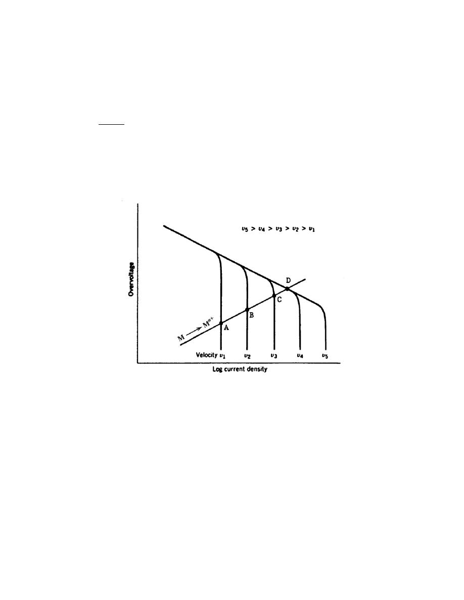
Excerpts from this work may be reproduced by instructors for distribution on a not-for-profit basis for testing or instructional purposes only to
students enrolled in courses for which the textbook has been adopted. Any other reproduction or translation of this work beyond that permitted
by Sections 107 or 108 of the 1976 United States Copyright Act without the permission of the copyright owner is unlawful.
17.19 The influence of increasing solution velocity on the overvoltage-versus-log current density behavior
for a solution that experiences combined activation–concentration polarization is indicated in Figure 17.26. On the
basis of this behavior, make a schematic plot of corrosion rate versus solution velocity for the oxidation of a metal;
assume that the oxidation reaction is controlled by activation polarization.
Solution
This problem asks that we make a schematic plot of corrosion rate versus solution velocity. The reduction
reaction is controlled by combined activation-concentration polarization for which the overvoltage versus logarithm
current density is presented in Figure 17.26. The oxidation of the metal is controlled by activation polarization,
such that the electrode kinetic behavior for the combined reactions would appear schematically as shown below.
Thus, the plot of corrosion rate versus solution velocity would be as
Excerpts from this work may be reproduced by instructors for distribution on a not-for-profit basis for testing or instructional purposes only to
students enrolled in courses for which the textbook has been adopted. Any other reproduction or translation of this work beyond that permitted
by Sections 107 or 108 of the 1976 United States Copyright Act without the permission of the copyright owner is unlawful.
The corrosion rate initially increases with increasing solution velocity (for velocities v
1
, v
2
, and v
3
), corresponding
to intersections in the concentration polarization regions for the reduction reaction. However, for the higher
solution velocities (v
4
and v
5
), the metal oxidation line intersects the reduction reaction curve in the linear activation
polarization region, and, thus, the reaction becomes independent of solution velocity.

Excerpts from this work may be reproduced by instructors for distribution on a not-for-profit basis for testing or instructional purposes only to
students enrolled in courses for which the textbook has been adopted. Any other reproduction or translation of this work beyond that permitted
by Sections 107 or 108 of the 1976 United States Copyright Act without the permission of the copyright owner is unlawful.
Passivity
17.20 Briefly describe the phenomenon of passivity. Name two common types of alloy that passivate.
Solution
Passivity is the loss of chemical reactivity, under particular environmental conditions, of normally active
metals and alloys. Stainless steels and aluminum alloys often passivate.

Excerpts from this work may be reproduced by instructors for distribution on a not-for-profit basis for testing or instructional purposes only to
students enrolled in courses for which the textbook has been adopted. Any other reproduction or translation of this work beyond that permitted
by Sections 107 or 108 of the 1976 United States Copyright Act without the permission of the copyright owner is unlawful.
17.21 Why does chromium in stainless steels make them more corrosion resistant in many environments
than plain carbon steels?
Solution
The chromium in stainless steels causes a very thin and highly adherent surface coating to form over the
surface of the alloy, which protects it from further corrosion. For plain carbon steels, rust, instead of this adherent
coating, forms.

Excerpts from this work may be reproduced by instructors for distribution on a not-for-profit basis for testing or instructional purposes only to
students enrolled in courses for which the textbook has been adopted. Any other reproduction or translation of this work beyond that permitted
by Sections 107 or 108 of the 1976 United States Copyright Act without the permission of the copyright owner is unlawful.
Forms of Corrosion
17.22 For each form of corrosion, other than uniform, do the following:
(a) Describe why, where, and the conditions under which the corrosion occurs.
(b) Cite three measures that may be taken to prevent or control it.
For each of the forms of corrosion, the conditions under which it occurs, and measures that may be taken to
prevent or control it are outlined in Section 17.7.

Excerpts from this work may be reproduced by instructors for distribution on a not-for-profit basis for testing or instructional purposes only to
students enrolled in courses for which the textbook has been adopted. Any other reproduction or translation of this work beyond that permitted
by Sections 107 or 108 of the 1976 United States Copyright Act without the permission of the copyright owner is unlawful.
17.23 Briefly explain why cold-worked metals are more susceptible to corrosion than noncold-worked
metals.
Solution
Cold-worked metals are more susceptible to corrosion than noncold-worked metals because of the
increased dislocation density for the latter. The region in the vicinity of a dislocation that intersects the surface is at
a higher energy state, and, therefore, is more readily attacked by a corrosive solution.

Excerpts from this work may be reproduced by instructors for distribution on a not-for-profit basis for testing or instructional purposes only to
students enrolled in courses for which the textbook has been adopted. Any other reproduction or translation of this work beyond that permitted
by Sections 107 or 108 of the 1976 United States Copyright Act without the permission of the copyright owner is unlawful.
17.24 Briefly explain why, for a small anode-to-cathode area ratio, the corrosion rate will be higher than
for a large ratio.
Solution
For a small anode-to-cathode area ratio, the corrosion rate will be higher than for a large ratio. The reason
for this is that for some given current flow associated with the corrosion reaction, for a small area ratio the current
density at the anode will be greater than for a large ratio. The corrosion rate is proportional to the current density (i)
according to Equation 17.24.

Excerpts from this work may be reproduced by instructors for distribution on a not-for-profit basis for testing or instructional purposes only to
students enrolled in courses for which the textbook has been adopted. Any other reproduction or translation of this work beyond that permitted
by Sections 107 or 108 of the 1976 United States Copyright Act without the permission of the copyright owner is unlawful.
17.25 For a concentration cell, briefly explain why corrosion occurs at that region having the lower
concentration.
Solution
For a concentration cell, corrosion occurs at that region having the lower concentration. In order to explain
this phenomenon let us consider an electrochemical cell consisting of two divalent metal M electrodes each of
which is immersed in a solution containing a different concentration of its M
2+
ion; let us designate the low and
high concentrations of M
2+
as
[ M
L
2
+
]
and
[ M
H
2
+
]
, respectively. Now assuming that reduction and oxidation
reactions occur in the high- and low-concentration solutions, respectively, let us determine the cell potential in terms
of the two [M
2+
]'s; if this potential is positive then we have chosen the solutions in which the reduction and
oxidation reactions appropriately.
Thus, the two half-reactions in the form of Equations 17.16 are
M
H
2+
+ 2e
-
→ M
V
M
M
→ M
L
2+
+ 2e
-
−V
M
Whereas the overall cell reaction is
M
H
2+
+ M
→ M + M
L
2+
From Equation 17.19, this yields a cell potential of
∆V = V
M
− V
M
−
RT
nF
ln
[ M
L
2
+
]
[ M
H
2
+
]
=
−
RT
nF
ln
[ M
L
2
+
]
[ M
H
2
+
]
Inasmuch as
[ M
L
2
+
]
< [M
H
2
+
] then the natural logarithm of the
[ M
2
+
] ratio is negative, which yields a positive
value for
∆V. This means that the electrochemical reaction is spontaneous as written, or that oxidation occurs at the
electrode having the lower M
2+
concentration.

Excerpts from this work may be reproduced by instructors for distribution on a not-for-profit basis for testing or instructional purposes only to
students enrolled in courses for which the textbook has been adopted. Any other reproduction or translation of this work beyond that permitted
by Sections 107 or 108 of the 1976 United States Copyright Act without the permission of the copyright owner is unlawful.
Corrosion Prevention
17.26 (a) What are inhibitors?
(b) What possible mechanisms account for their effectiveness?
Solution
(a) Inhibitors are substances that, when added to a corrosive environment in relatively low concentrations,
decrease the environment's corrosiveness.
(b) Possible mechanisms that account for the effectiveness of inhibitors are: (1) elimination of a
chemically active species in the solution; (2) attachment of inhibitor molecules to the corroding surface so as to
interfere with either the oxidation or reduction reaction; and (3) the formation of a very thin and protective coating
on the corroding surface.

Excerpts from this work may be reproduced by instructors for distribution on a not-for-profit basis for testing or instructional purposes only to
students enrolled in courses for which the textbook has been adopted. Any other reproduction or translation of this work beyond that permitted
by Sections 107 or 108 of the 1976 United States Copyright Act without the permission of the copyright owner is unlawful.
17.27 Briefly describe the two techniques that are used for galvanic protection.
Solution
Descriptions of the two techniques used for galvanic protection are as follows:
(1) A sacrificial anode is electrically coupled to the metal piece to be protected, which anode is also
situated in the corrosion environment. The sacrificial anode is a metal or alloy that is chemically more reactive in
the particular environment. It (the anode) preferentially oxidizes, and, upon giving up electrons to the other metal,
protects it from electrochemical corrosion.
(2) An impressed current from an external dc power source provides excess electrons to the metallic
structure to be protected.

Excerpts from this work may be reproduced by instructors for distribution on a not-for-profit basis for testing or instructional purposes only to
students enrolled in courses for which the textbook has been adopted. Any other reproduction or translation of this work beyond that permitted
by Sections 107 or 108 of the 1976 United States Copyright Act without the permission of the copyright owner is unlawful.
Oxidation
17.28 For each of the metals listed in the table, compute the Pilling–Bedworth ratio. Also, on the basis of
this value, specify whether or not you would expect the oxide scale that forms on the surface to be protective, and
then justify your decision. Density data for both the metal and its oxide are also tabulated.
Metal
Metal Density
(g/cm
3
)
Metal Oxide
Oxide Density
(g/cm
3
)
Zr
6.51
ZrO
2
5.89
Sn
7.30
SnO
2
6.95
Bi
9.80
Bi
2
O
3
8.90
Solution
With this problem we are given, for three metals, their densities, oxide chemical formulas, and oxide
densities, and are asked to compute the Pilling-Bedworth ratios, and then to specify whether or not the oxide scales
that form will be protective. The general form of the equation used to calculate this ratio is Equation 17.32 (or
Equation 17.33). For zirconium, oxidation occurs by the reaction
Zr + O
2
→ ZrO
2
and therefore, from Equation 17.32
P
− B ratio =
A
ZrO
2
ρ
Zr
A
Zr
ρ
ZrO
2
=
(123.22 g/mol)
(
6.51 g/cm
3
)
(91.22 g/mol)
(
5.89 g/cm
3
)
= 1.49
Thus, this would probably be a protective oxide film since the P-B ratio lies between one and two.
The oxidation reaction for Sn is just
Sn + O
2
→ SnO
2
and the P-B ratio is (Equation 17.32)
Excerpts from this work may be reproduced by instructors for distribution on a not-for-profit basis for testing or instructional purposes only to
students enrolled in courses for which the textbook has been adopted. Any other reproduction or translation of this work beyond that permitted
by Sections 107 or 108 of the 1976 United States Copyright Act without the permission of the copyright owner is unlawful.
P
− B ratio =
A
SnO
2
ρ
Sn
A
Sn
ρ
SnO
2
=
(150.71 g/mol)
(
7.30 g/cm
3
)
(118.71 g/mol)
(
6.95 g/cm
3
)
= 1.33
Hence, the film would most likely be protective since the ratio lies between one and two.
Now for Bi, the reaction for its oxidation is
2Bi +
3
2
O
2
→ Bi
2
O
3
and the P-B ratio is (Equation 17.33)
P
− B ratio =
A
Bi
2
O
3
ρ
Bi
(2) A
Bi
ρ
Bi
2
O
3
=
(465.96 g/mol)
(
9.80 g/cm
3
)
(2)(208.98 g/mol)
(
8.90 g/cm
3
)
= 1.23
Thus, the Bi
2
O
3
film would probably be protective since the ratio is between one and two.

Excerpts from this work may be reproduced by instructors for distribution on a not-for-profit basis for testing or instructional purposes only to
students enrolled in courses for which the textbook has been adopted. Any other reproduction or translation of this work beyond that permitted
by Sections 107 or 108 of the 1976 United States Copyright Act without the permission of the copyright owner is unlawful.
17.29 According to Table 17.3, the oxide coating that forms on silver should be nonprotective, and yet Ag
does not oxidize appreciably at room temperature and in air. How do you explain this apparent discrepancy?
Solution
Silver does not oxidize appreciably at room temperature and in air even though, according to Table 17.3,
the oxide coating should be nonprotective. The reason for this is that the oxidation of silver in air is not
thermodynamically favorable; therefore, the lack of a reaction is independent of whether or not a protective scale
forms.

Excerpts from this work may be reproduced by instructors for distribution on a not-for-profit basis for testing or instructional purposes only to
students enrolled in courses for which the textbook has been adopted. Any other reproduction or translation of this work beyond that permitted
by Sections 107 or 108 of the 1976 United States Copyright Act without the permission of the copyright owner is unlawful.
17.30 In the table, weight gain-time data for the oxidation of copper at an elevated temperature are
tabulated.
W (mg/cm
2
)
Time (min)
0.316
15
0.524
50
0.725
100
(a) Determine whether the oxidation kinetics obey a linear, parabolic, or logarithmic rate expression.
(b) Now compute W after a time of 450 min.
Solution
For this problem we are given weight gain-time data for the oxidation of Cu at an elevated temperature.
(a) We are first asked to determine whether the oxidation kinetics obey a parabolic, linear, or logarithmic
rate expression, which expressions are represented by Equations 17.34, 17.35, and 17.36, respectively. One way to
make this determination is by trial and error. Let us assume that the parabolic relationship is valid; that is from
Equation 17.34
W
2
= K
1
t + K
2
which means that we may establish three simultaneous equations using the three sets of given W and t values, then
using two combinations of two pairs of equations, solve for K
1
and K
2
; if K
1
and K
2
have the same values for both
solutions, then the kinetics are parabolic. If the values are not identical then the other kinetic relationships need to
be explored. Thus, the three equations are
(0.316)
2
= 0.100 = 15K
1
+ K
2
(0.524)
2
= 0.275 = 50K
1
+ K
2
(0.725)
2
= 0.526 = 100K
1
+ K
2
From the first two equations K
1
= 5
× 10
-3
and K
2
= 0.025; these same two values are obtained using the last two
equations. Hence, the oxidation rate law is parabolic.
(b) Since a parabolic relationship is valid, this portion of the problem calls for us to determine W after a
total time of 450 min. Again, using Equation 17.34 and the values of K
1
and K
2
W
2
= K
1
t + K
2

Excerpts from this work may be reproduced by instructors for distribution on a not-for-profit basis for testing or instructional purposes only to
students enrolled in courses for which the textbook has been adopted. Any other reproduction or translation of this work beyond that permitted
by Sections 107 or 108 of the 1976 United States Copyright Act without the permission of the copyright owner is unlawful.
= (5
× 10
-3
)(450 min) + 0.025 = 2.28
Or W =
2.28 = 1.51 mg/cm
2
.

Excerpts from this work may be reproduced by instructors for distribution on a not-for-profit basis for testing or instructional purposes only to
students enrolled in courses for which the textbook has been adopted. Any other reproduction or translation of this work beyond that permitted
by Sections 107 or 108 of the 1976 United States Copyright Act without the permission of the copyright owner is unlawful.
17.31 In the table, weight gain–time data for the oxidation of some metal at an elevated temperature are
tabulated.
W (mg/cm
2
)
Time (min)
4.66
20
11.7
50
41.1
135
(a) Determine whether the oxidation kinetics obey a linear, parabolic, or logarithmic rate expression.
(b) Now compute W after a time of 1000 min.
Solution
For this problem we are given weight gain-time data for the oxidation of some metal at an elevated
temperature.
(a) We are first asked to determine whether the oxidation kinetics obey a linear, parabolic, or logarithmic
rate expression, which expressions are described by Equations 17.35, 17.34, and 17.36, respectively. One way to
make this determination is by trial and error. Let us assume that the rate expression is linear, that is from Equation
17.35
W = K
3
t
which means that we may establish three simultaneous equations using the three sets of given W and t values, then
solve for K
3
for each; if K
3
is the same for all three cases, then the rate law is linear. If the values are not the same
then the other kinetic relationships need to be explored. Thus, the three equations are
4.66 = 20 K
3
11.7 = 50 K
3
41.1 = 175K
3
In all three instances the value of K
3
is about equal to 0.234, which means the oxidation rate obeys a linear
expression.
(b) Now we are to calculate W after a time of 1000 min; thus
W = K
3
t = (0.234)(1000 min) = 234 mg/cm
2

Excerpts from this work may be reproduced by instructors for distribution on a not-for-profit basis for testing or instructional purposes only to
students enrolled in courses for which the textbook has been adopted. Any other reproduction or translation of this work beyond that permitted
by Sections 107 or 108 of the 1976 United States Copyright Act without the permission of the copyright owner is unlawful.
17.32 In the table, weight gain–time data for the oxidation of some metal at an elevated temperature are
tabulated.
W (mg/cm
2
)
Time (min)
1.90
25
3.76
75
6.40
250
(a) Determine whether the oxidation kinetics obey a linear, parabolic, or logarithmic rate expression.
(b) Now compute W after a time of 3500 min.
Solution
For this problem we are given weight gain-time data for the oxidation of some metal at an elevated
temperature.
(a) We are first asked to determine whether the oxidation kinetics obey a linear, parabolic, or logarithmic
rate expression, which expressions are described by Equations 17.35, 17.34, and 17.36, respectively. One way to
make this determination is by trial and error. Let us assume that the kinetic rate is parabolic, that is from Equation
17.34
W
2
= K
1
t + K
2
which means that we may establish three simultaneous equations using the three sets of given W and t values, then
using two combinations of two pairs of equations, solve for K
1
and K
2
; if K
1
and K
2
have the same values for both
solutions, then the weight gain-time relationships are parabolic. If the values are not the same then the other kinetic
relationships need to be explored. Thus, the three equations are
(1.90)
2
= 3.610 = 25K
1
+ K
2
(3.67)
2
= 13.47 = 75K
1
+ K
2
(6.40)
2
= 40.96 = 250K
1
+ K
2
From the first two equations K
1
= 0.197 and K
2
= -1.32; while from the second and third equations K
1
= 0.157 and
K
2
= 1.689. Thus, a parabolic rate expression is not obeyed by this reaction.
Let us now investigate linear kinetics in the same manner, using Equation 17.35, W = K
3
t. The three
equations are thus
1.90 = 25K
3
3.67 = 75K
3

Excerpts from this work may be reproduced by instructors for distribution on a not-for-profit basis for testing or instructional purposes only to
students enrolled in courses for which the textbook has been adopted. Any other reproduction or translation of this work beyond that permitted
by Sections 107 or 108 of the 1976 United States Copyright Act without the permission of the copyright owner is unlawful.
6.40 = 250K
3
And three K
3
values may be computed (one for each equation) which are 7.60
× 10
-2
, 4.89
× 10
-2
, and 2.56
× 10
-2
.
Since these K
3
values are all different, a linear rate law is not a possibility, and, by process of elimination, a
logarithmic expression is obeyed.
(b) In order to determine the value of W after 3500 min, it is first necessary that we solve for the K
4
, K
5
,
and K
6
constants of Equation 17.36. One way this may be accomplished is to use an equation solver. In some
instances it is desirable to express Equation 17.36 in exponential form, as
K
5
+ K
6
= 10
W /K
4
For some solvers, using the above expression, the following instructions can be used:
K5 *t1 + K6 = 10^(W1/K4)
K5 *t2 + K6 = 10^(W2/K4)
K5 *t3 + K6 = 10^(W3/K4)
t1 = 25;
W1 = 1.90
t2 = 75;
W2 = 3.67
t3 = 250;
W3 = 6.40
The resulting solutions—i.e., values for the K parameters—are
K
4
= 6.50
K
5
= 0.0342
K
6
= 1.1055
Now solving Equation 17.36 for W at a time of 3500 min
W = K
4
log
(
K
5
t
+ K
6
)
= 6.50 log (0.0342 )(3500 min)
+ 1.1055
[
]
= 13.53 mg/cm
2

Excerpts from this work may be reproduced by instructors for distribution on a not-for-profit basis for testing or instructional purposes only to
students enrolled in courses for which the textbook has been adopted. Any other reproduction or translation of this work beyond that permitted
by Sections 107 or 108 of the 1976 United States Copyright Act without the permission of the copyright owner is unlawful.
DESIGN PROBLEMS
17.D1 A brine solution is used as a cooling medium in a steel heat exchanger. The brine is circulated
within the heat exchanger and contains some dissolved oxygen. Suggest three methods, other than cathodic
protection, for reducing corrosion of the steel by the brine. Explain the rationale for each suggestion.
Solution
Possible methods that may be used to reduce corrosion of the heat exchanger by the brine solution are as
follows:
(1) Reduce the temperature of the brine; normally, the rate of a corrosion reaction increases with
increasing temperature.
(2) Change the composition of the brine; the corrosion rate is often quite dependent on the composition of
the corrosion environment.
(3) Remove as much dissolved oxygen as possible. Under some circumstances, the dissolved oxygen may
form bubbles, which can lead to erosion-corrosion damage.
(4) Minimize the number of bends and/or changes in pipe contours in order to minimize erosion-corrosion.
(5) Add inhibitors.
(6) Avoid connections between different metal alloys.

Excerpts from this work may be reproduced by instructors for distribution on a not-for-profit basis for testing or instructional purposes only to
students enrolled in courses for which the textbook has been adopted. Any other reproduction or translation of this work beyond that permitted
by Sections 107 or 108 of the 1976 United States Copyright Act without the permission of the copyright owner is unlawful.
17.D2 Suggest an appropriate material for each of the following applications, and, if necessary,
recommend corrosion prevention measures that should be taken. Justify your suggestions.
(a) Laboratory bottles to contain relatively dilute solutions of nitric acid
(b) Barrels to contain benzene
(c) Pipe to transport hot alkaline (basic) solutions
(d) Underground tanks to store large quantities of high-purity water
(e) Architectural trim for high-rise buildings
Solution
This question asks that we suggest appropriate materials, and if necessary, recommend corrosion
prevention measures that should be taken for several specific applications. These are as follows:
(a) Laboratory bottles to contain relatively dilute solutions of nitric acid. Probably the best material for
this application would be polytetrafluoroethylene (PTFE). The reasons for this are: (1) it is flexible and will not
easily break if dropped; and (2) PTFE is resistant to this type of acid, as noted in Table 17.4.
(b) Barrels to contain benzene. Poly(ethylene terephthalate) (PET) would be suited for this application,
since it is resistant to degradation by benzene (Table 17.4), and is less expensive than the other two materials listed
in Table 17.4 (see Appendix C).
(c) Pipe to transport hot alkaline (basic) solutions. The best material for this application would probably
be a nickel alloy (Section 13.3). Polymeric materials listed in Table 17.4 would not be suitable inasmuch as the
solutions are hot.
(d) Underground tanks to store large quantities of high-purity water. The outside of the tanks should
probably be some type of low-carbon steel that is cathodically protected (Sections 17.8 and 17.9). Inside the steel
shell should be coated with an inert polymeric material; polytetrafluoroethylene or some other fluorocarbon would
probably be the material of choice (Table 17.4).
(e) Architectural trim for high-rise buildings. The most likely candidate for this application would
probably be an aluminum alloy. Aluminum and its alloys are relatively corrosion resistant in normal atmospheres
(Section 16.8), retain their lustrous appearance, and are relatively inexpensive (Appendix C).

Excerpts from this work may be reproduced by instructors for distribution on a not-for-profit basis for testing or instructional purposes only to
students enrolled in courses for which the textbook has been adopted. Any other reproduction or translation of this work beyond that permitted
by Sections 107 or 108 of the 1976 United States Copyright Act without the permission of the copyright owner is unlawful.
17.D3 Each student (or group of students) is to find a real-life corrosion problem that has not been solved,
conduct a thorough investigation as to the cause(s) and type(s) of corrosion, and, finally, propose possible solutions
for the problem, indicating which of the solutions is best and why. Submit a report that addresses the above issues.
Each student or group of students is to submit their own report on a corrosion problem investigation that
was conducted.

Excerpts from this work may be reproduced by instructors for distribution on a not-for-profit basis for testing or instructional purposes only to
students enrolled in courses for which the textbook has been adopted. Any other reproduction or translation of this work beyond that permitted
by Sections 107 or 108 of the 1976 United States Copyright Act without the permission of the copyright owner is unlawful.
CHAPTER 18
ELECTRICAL PROPERTIES
PROBLEM SOLUTIONS
Ohm’s Law
Electrical Conductivity
18.1 (a) Compute the electrical conductivity of a 5.1-mm (0.2-in.) diameter cylindrical silicon specimen 51
mm (2 in.) long in which a current of 0.1 A passes in an axial direction. A voltage of 12.5 V is measured across two
probes that are separated by 38 mm (1.5 in.).
(b) Compute the resistance over the entire 51 mm (2 in.) of the specimen.
Solution
This problem calls for us to compute the electrical conductivity and resistance of a silicon specimen.
(a) We use Equations 18.3 and 18.4 for the conductivity, as
σ =
1
ρ
=
Il
VA
=
Il
V
π
d
2
2
And, incorporating values for the several parameters provided in the problem statement, leads to
σ =
(0.1 A)
(
38
× 10
−3
m
)
(12.5 V)(
π)
5.1
× 10
−3
m
2
2
= 14.9 (
Ω - m)
-1
(b) The resistance, R, may be computed using Equations 18.2 and 18.4, as
R =
ρl
A
=
l
σA
=
l
σπ
d
2
2

Excerpts from this work may be reproduced by instructors for distribution on a not-for-profit basis for testing or instructional purposes only to
students enrolled in courses for which the textbook has been adopted. Any other reproduction or translation of this work beyond that permitted
by Sections 107 or 108 of the 1976 United States Copyright Act without the permission of the copyright owner is unlawful.
=
51
× 10
−3
m
14.9 (
Ω − m)
−1
[
]
(
π)
5.1
× 10
−3
m
2
2
= 168
Ω
Excerpts from this work may be reproduced by instructors for distribution on a not-for-profit basis for testing or instructional purposes only to
students enrolled in courses for which the textbook has been adopted. Any other reproduction or translation of this work beyond that permitted
by Sections 107 or 108 of the 1976 United States Copyright Act without the permission of the copyright owner is unlawful.
18.2 A copper wire 100 m long must experience a voltage drop of less than 1.5 V when a current of 2.5 A
passes through it. Using the data in Table 18.1, compute the minimum diameter of the wire.
Solution
For this problem, given that a copper wire 100 m long must experience a voltage drop of less than 1.5 V
when a current of 2.5 A passes through it, we are to compute the minimum diameter of the wire. Combining
Equations 18.3 and 18.4 and solving for the cross-sectional area A leads to
A =
Il
ρ
V
=
Il
V
σ
From Table 18.1, for copper
σ = 6.0 × 10
7
(
Ω-m)
-1
. Furthermore, inasmuch as
A =
π
d
2
2
for a cylindrical wire,
then
π
d
2
2
=
Il
V
σ
or
d =
4 Il
πVσ
When values for the several parameters given in the problem statement are incorporated into this expression, we get
d =
(4)(2.5 A)(100 m)
(
π)(1.5 V) 6.0 × 10
7
(
Ω − m)
−1
[
]
= 1.88
× 10
-3
m = 1.88 mm

Excerpts from this work may be reproduced by instructors for distribution on a not-for-profit basis for testing or instructional purposes only to
students enrolled in courses for which the textbook has been adopted. Any other reproduction or translation of this work beyond that permitted
by Sections 107 or 108 of the 1976 United States Copyright Act without the permission of the copyright owner is unlawful.
18.3 An aluminum wire 4 mm in diameter is to offer a resistance of no more than 2.5
Ω. Using the data in
Table 18.1, compute the maximum wire length.
Solution
This problem asks that we compute, for an aluminum wire 4 mm in diameter, the maximum length such
that the resistance will not exceed 2.5
Ω. From Table 18.1 for aluminum, σ = 3.8 × 10
7
(
Ω-m)
-1
. If d is the
diameter then, combining Equations 18.2 and 18.4 leads to
l =
RA
ρ
= R
σA = Rσπ
d
2
2
= (2.5
Ω) 3.8 × 10
7
(
Ω − m)
−1
[
]
(
π)
4
× 10
−3
m
2
2
= 1194 m

Excerpts from this work may be reproduced by instructors for distribution on a not-for-profit basis for testing or instructional purposes only to
students enrolled in courses for which the textbook has been adopted. Any other reproduction or translation of this work beyond that permitted
by Sections 107 or 108 of the 1976 United States Copyright Act without the permission of the copyright owner is unlawful.
18.4 Demonstrate that the two Ohm’s law expressions, Equations 18.1 and 18.5, are equivalent.
Solution
Let us demonstrate, by appropriate substitution and algebraic manipulation, that Equation 18.5 may be
made to take the form of Equation 18.1. Now, Equation 18.5 is just
J =
σE
(In this equation we represent the electric field with an “E”.) But, by definition, J is just the current density, the
current per unit cross-sectional area, or
J
=
I
A
. Also, the electric field is defined by
E
=
V
l
. And, substituting
these expressions into Equation 18.5 leads to
I
A
=
σ
V
l
But, from Equations 18.2 and 18.4
σ =
l
RA
and
I
A
=
l
RA
V
l
Solving for V from this expression gives V = IR, which is just Equation 18.1.

Excerpts from this work may be reproduced by instructors for distribution on a not-for-profit basis for testing or instructional purposes only to
students enrolled in courses for which the textbook has been adopted. Any other reproduction or translation of this work beyond that permitted
by Sections 107 or 108 of the 1976 United States Copyright Act without the permission of the copyright owner is unlawful.
18.5 (a) Using the data in Table 18.1, compute the resistance of a copper wire 3 mm (0.12 in.) in diameter
and 2 m (78.7 in.) long. (b) What would be the current flow if the potential drop across the ends of the wire is 0.05
V? (c) What is the current density? (d) What is the magnitude of the electric field across the ends of the wire?
Solution
(a) In order to compute the resistance of this copper wire it is necessary to employ Equations 18.2 and
18.4. Solving for the resistance in terms of the conductivity,
R =
ρ l
A
=
l
σA
=
l
σπ
d
2
2
From Table 18.1, the conductivity of copper is 6.0
× 10
7
(
Ω-m)
-1
, and
R =
l
σπ
d
2
2
=
2 m
6.0
× 10
7
(
Ω − m)
−1
[
]
(
π)
3
× 10
−3
m
2
2
= 4.7
× 10
-3
Ω
(b) If V = 0.05 V then, from Equation 18.1
I =
V
R
=
0.05 V
4.7
× 10
−3
Ω
= 10.6 A
(c) The current density is just
J =
I
A
=
I
π
d
2
2
=
10.6 A
π
3
× 10
−3
m
2
2
= 1.5
× 10
6
A/m
2
(d) The electric field is just
E =
V
l
=
0.05 V
2 m
= 2.5
× 10
-2
V/m

Excerpts from this work may be reproduced by instructors for distribution on a not-for-profit basis for testing or instructional purposes only to
students enrolled in courses for which the textbook has been adopted. Any other reproduction or translation of this work beyond that permitted
by Sections 107 or 108 of the 1976 United States Copyright Act without the permission of the copyright owner is unlawful.
Electronic and Ionic Conduction
18.6 What is the distinction between electronic and ionic conduction?
Solution
When a current arises from a flow of electrons, the conduction is termed electronic; for ionic conduction,
the current results from the net motion of charged ions.

Excerpts from this work may be reproduced by instructors for distribution on a not-for-profit basis for testing or instructional purposes only to
students enrolled in courses for which the textbook has been adopted. Any other reproduction or translation of this work beyond that permitted
by Sections 107 or 108 of the 1976 United States Copyright Act without the permission of the copyright owner is unlawful.
Energy Band Structures in Solids
18.7 How does the electron structure of an isolated atom differ from that of a solid material?
Solution
For an isolated atom, there exist discrete electron energy states (arranged into shells and subshells); each
state may be occupied by, at most, two electrons, which must have opposite spins. On the other hand, an electron
band structure is found for solid materials; within each band exist closely spaced yet discrete electron states, each
of which may be occupied by, at most, two electrons, having opposite spins. The number of electron states in each
band will equal the total number of corresponding states contributed by all of the atoms in the solid.

Excerpts from this work may be reproduced by instructors for distribution on a not-for-profit basis for testing or instructional purposes only to
students enrolled in courses for which the textbook has been adopted. Any other reproduction or translation of this work beyond that permitted
by Sections 107 or 108 of the 1976 United States Copyright Act without the permission of the copyright owner is unlawful.
Conduction in Terms of Band and Atomic Bonding Models
18.8 In terms of electron energy band structure, discuss reasons for the difference in electrical
conductivity between metals, semiconductors, and insulators.
Solution
For metallic materials, there are vacant electron energy states adjacent to the highest filled state; thus, very
little energy is required to excite large numbers of electrons into conducting states. These electrons are those that
participate in the conduction process, and, because there are so many of them, metals are good electrical conductors.
There are no empty electron states adjacent to and above filled states for semiconductors and insulators, but
rather, an energy band gap across which electrons must be excited in order to participate in the conduction process.
Thermal excitation of electrons will occur, and the number of electrons excited will be less than for metals, and will
depend on the band gap energy. For semiconductors, the band gap is narrower than for insulators; consequently, at
a specific temperature more electrons will be excited for semiconductors, giving rise to higher conductivities.

Excerpts from this work may be reproduced by instructors for distribution on a not-for-profit basis for testing or instructional purposes only to
students enrolled in courses for which the textbook has been adopted. Any other reproduction or translation of this work beyond that permitted
by Sections 107 or 108 of the 1976 United States Copyright Act without the permission of the copyright owner is unlawful.
Electron Mobility
18.9 Briefly tell what is meant by the drift velocity and mobility of a free electron.
Solution
The drift velocity of a free electron is the average electron velocity in the direction of the force imposed by
an electric field.
The mobility is the proportionality constant between the drift velocity and the electric field. It is also a
measure of the frequency of scattering events (and is inversely proportional to the frequency of scattering).

Excerpts from this work may be reproduced by instructors for distribution on a not-for-profit basis for testing or instructional purposes only to
students enrolled in courses for which the textbook has been adopted. Any other reproduction or translation of this work beyond that permitted
by Sections 107 or 108 of the 1976 United States Copyright Act without the permission of the copyright owner is unlawful.
18.10 (a) Calculate the drift velocity of electrons in germanium at room temperature and when the
magnitude of the electric field is 1000 V/m. (b) Under these circumstances, how long does it take an electron to
traverse a 25-mm (1-in.) length of crystal?
Solution
(a) The drift velocity of electrons in Ge may be determined using Equation 18.7. Since the room
temperature mobility of electrons is 0.38 m
2
/V-s (Table 18.3), and the electric field is 1000 V/m (as stipulated in the
problem statement),
v
d
=
µ
e
E
=
(
0.38 m
2
/V - s
)
(1000 V/m) = 380 m/s
(b) The time, t, required to traverse a given length, l (= 25 mm), is just
t =
l
v
d
=
25
× 10
−3
m
380 m /s
= 6.6
× 10
-5
s
Excerpts from this work may be reproduced by instructors for distribution on a not-for-profit basis for testing or instructional purposes only to
students enrolled in courses for which the textbook has been adopted. Any other reproduction or translation of this work beyond that permitted
by Sections 107 or 108 of the 1976 United States Copyright Act without the permission of the copyright owner is unlawful.
18.11 At room temperature the electrical conductivity and the electron mobility for copper are 6.0
× 10
7
(
Ω-m)
-1
and 0.0030 m
2
/V-s, respectively. (a) Compute the number of free electrons per cubic meter for copper at
room temperature. (b) What is the number of free electrons per copper atom? Assume a density of 8.9 g/cm
3
.
Solution
(a) The number of free electrons per cubic meter for copper at room temperature may be computed using
Equation 18.8 as
n =
σ
| e | µ
e
=
6.0
× 10
7
(
Ω − m)
−1
(
1.602
× 10
−19
C
)(
0.003 m
2
/V - s
)
= 1.25
× 10
29
m
-3
(b) In order to calculate the number of free electrons per copper atom, we must first determine the number
of copper atoms per cubic meter, N
Cu
. From Equation 4.2 (and using the atomic weight value for Cu found inside
the front cover—viz. 63.55 g/mol)
N
Cu
=
N
A
′
ρ
A
Cu
=
(
6.022
× 10
23
atoms / mol
)(
8.9 g/cm
3
)(
10
6
cm
3
/ m
3
)
63.55 g/mol
= 8.43
× 10
28
m
-3
(Note: in the above expression, density is represented by
ρ' in order to avoid confusion with resistivity which is
designated by
ρ.) And, finally, the number of free electrons per aluminum atom is just n/N
Cu
n
N
Cul
=
1.25
× 10
29
m
−3
8.43
× 10
28
m
−3
= 1.48

Excerpts from this work may be reproduced by instructors for distribution on a not-for-profit basis for testing or instructional purposes only to
students enrolled in courses for which the textbook has been adopted. Any other reproduction or translation of this work beyond that permitted
by Sections 107 or 108 of the 1976 United States Copyright Act without the permission of the copyright owner is unlawful.
18.12 (a) Calculate the number of free electrons per cubic meter for gold assuming that there are 1.5 free
electrons per gold atom. The electrical conductivity and density for Au are 4.3
× 10
7
(
Ω-m)
-1
and 19.32 g/cm
3
,
respectively. (b) Now compute the electron mobility for Au.
Solution
(a) This portion of the problem asks that we calculate, for gold, the number of free electrons per cubic
meter (n) given that there are 1.5 free electrons per gold atom, that the electrical conductivity is 4.3
× 10
7
(
Ω-m)
-1
,
and that the density
(
ρ
Au
'
)
is 19.32 g/cm
3
. (Note: in this discussion, the density of silver is represented by
ρ
Au
'
in
order to avoid confusion with resistivity which is designated by
ρ.) Since n = 1.5N
Au
, and N
Au
is defined in
Equation 4.2 (and using the atomic weight of Au found inside the front cover—viz 196.97 g/mol), then
n = 1.5N
Au
= 1.5
ρ
Au
'
N
A
A
Au
= 1.5
(
19.32 g/cm
3
)(
6.022
× 10
23
atoms / mol
)
196.97 g/mol
= 8.86
× 10
22
cm
-3
= 8.86
× 10
28
m
-3
(b) Now we are asked to compute the electron mobility,
µ
e
. Using Equation 18.8
µ
e
=
σ
n
| e |
=
4.3
× 10
7
(
Ω − m)
−1
(
8.86
× 10
28
m
−3
)(
1.602
× 10
−19
C
)
= 3.03
× 10
-3
m
2
/V - s

Excerpts from this work may be reproduced by instructors for distribution on a not-for-profit basis for testing or instructional purposes only to
students enrolled in courses for which the textbook has been adopted. Any other reproduction or translation of this work beyond that permitted
by Sections 107 or 108 of the 1976 United States Copyright Act without the permission of the copyright owner is unlawful.
Electrical Resistivity of Metals
18.13 From Figure 18.38, estimate the value of A in Equation 18.11 for zinc as an impurity in copper–zinc
alloys.
Solution
We want to solve for the parameter A in Equation 18.11 using the data in Figure 18.38. From Equation
18.11
A =
ρ
i
c
i
(1
− c
i )
However, the data plotted in Figure 18.38 is the total resistivity,
ρ
total
, and includes both impurity (
ρ
i
) and thermal
(
ρ
t
) contributions (Equation 18.9). The value of
ρ
t
is taken as the resistivity at c
i
= 0 in Figure 18.38, which has a
value of 1.7
× 10
-8
(
Ω-m); this must be subtracted out. Below are tabulated values of A determined at c
i
= 0.10,
0.20, and 0.30, including other data that were used in the computations. (Note: the c
i
values were taken from the
upper horizontal axis of Figure 18.38, since it is graduated in atom percent zinc.)
c
i
1 – c
i
ρ
total
(
Ω-m)
ρ
i
(
Ω-m)
A (
Ω-m)
0.10
0.90
4.0
× 10
-8
2.3
× 10
-8
2.56
× 10
-7
0.20
0.80
5.4
× 10
-8
3.7
× 10
-8
2.31
× 10
-7
0.30
0.70
6.15
× 10
-8
4.45
× 10
-8
2.12
× 10
-7
So, there is a slight decrease of A with increasing c
i
.

Excerpts from this work may be reproduced by instructors for distribution on a not-for-profit basis for testing or instructional purposes only to
students enrolled in courses for which the textbook has been adopted. Any other reproduction or translation of this work beyond that permitted
by Sections 107 or 108 of the 1976 United States Copyright Act without the permission of the copyright owner is unlawful.
18.14 (a) Using the data in Figure 18.8, d
etermine the values of ρ
0
and a from Equation 18.10 for pure
copper. Take the temperature T to be in degrees Celsius. (b) Determine the value of A in Equation 18.11 for nickel
as an impurity in copper, using the data in Figure 18.8. (c) Using the results of parts (a) and (b), estimate the
electrical resistivity of copper containing 1.75 at% Ni at 100°C.
Solution
(a) Perhaps the easiest way to determine the values of
ρ
0
and a in Equation 18.10 for pure copper in
Figure 18.8, is to set up two simultaneous equations using two resistivity values (labeled
ρ
t1
and
ρ
t2
) taken at two
corresponding temperatures (T
1
and T
2
). Thus,
ρ
t1
=
ρ
0
+ aT
1
ρ
t2
=
ρ
0
+ aT
2
And solving these equations simultaneously lead to the following expressions for a and
ρ
0
:
a =
ρ
t1
− ρ
t2
T
1
− T
2
ρ
0
=
ρ
t1
− T
1
ρ
t1
− ρ
t 2
T
1
−T
2
=
ρ
t 2
− T
2
ρ
t1
− ρ
t2
T
1
− T
2
From Figure 18.8, let us take T
1
= –150
°C, T
2
= –50
°C, which gives ρ
t1
= 0.6
× 10
-8
(
Ω-m), and ρ
t2
= 1.25
× 10
-8
(
Ω-m). Therefore
a =
ρ
t1
− ρ
t2
T
1
− T
2
=
(
0.6
× 10
-8
)
−
(
1.25
× 10
-8
)
[
]
Ω - m
(
)
−150°C − (−50°C)
6.5
× 10
-11
(
Ω-m)/°C

Excerpts from this work may be reproduced by instructors for distribution on a not-for-profit basis for testing or instructional purposes only to
students enrolled in courses for which the textbook has been adopted. Any other reproduction or translation of this work beyond that permitted
by Sections 107 or 108 of the 1976 United States Copyright Act without the permission of the copyright owner is unlawful.
and
ρ
0
=
ρ
t1
− T
1
ρ
t1
− ρ
t 2
T
1
−T
2
=
(
0.6
× 10
-8
)
− (−150)
(
0.6
× 10
-8
)
−
(
1.25
× 10
-8
)
[
]
Ω - m
(
)
−150°C − (−50°C)
= 1.58
× 10
-8
(
Ω-m)
(b) For this part of the problem, we want to calculate A from Equation 18.11
ρ
i
= Ac
i
(1
− c
i
)
In Figure 18.8, curves are plotted for three c
i
values (0.0112, 0.0216, and 0.0332). Let us find A for each of these
c
i
's by taking a
ρ
total
from each curve at some temperature (say 0
°C) and then subtracting out ρ
i
for pure copper at
this same temperature (which is 1.7
× 10
-8
Ω-m). Below is tabulated values of A determined from these three c
i
values, and other data that were used in the computations.
c
i
1 – c
i
ρ
total
(
Ω-m)
ρ
i
(
Ω-m)
A (
Ω-m)
0.0112
0.989
3.0
× 10
-8
1.3
× 10
-8
1.17
× 10
-6
0.0216
0.978
4.2
× 10
-8
2.5
× 10
-8
1.18
× 10
-6
0.0332
0.967
5.5
× 10
-8
3.8
× 10
-8
1.18
× 10
-6
The average of these three A values is 1.18
× 10
-6
(
Ω-m).
(c) We use the results of parts (a) and (b) to estimate the electrical resistivity of copper containing 1.75
at% Ni (c
i
= 0.0175) at 100
°C. The total resistivity is just
ρ
total
=
ρ
t
+
ρ
i
Or incorporating the expressions for
ρ
t
and
ρ
i
from Equations 18.10 and 18.11, and the values of
ρ
0
, a, and A
determined above, leads to
ρ
total
= (
ρ
0
+ aT) + Ac
i
(1
− c
i
)

Excerpts from this work may be reproduced by instructors for distribution on a not-for-profit basis for testing or instructional purposes only to
students enrolled in courses for which the textbook has been adopted. Any other reproduction or translation of this work beyond that permitted
by Sections 107 or 108 of the 1976 United States Copyright Act without the permission of the copyright owner is unlawful.
=
{
1.58
× 10
-8
(
Ω - m) +
[
6.5
× 10
-11
(
Ω - m) /°C
]
(100
°C)
}
+
{
[
1.18
× 10
-6
(
Ω - m)
]
(0.0175) (1
− 0.0175)
}
= 4.25
× 10
-8
(
Ω-m)

Excerpts from this work may be reproduced by instructors for distribution on a not-for-profit basis for testing or instructional purposes only to
students enrolled in courses for which the textbook has been adopted. Any other reproduction or translation of this work beyond that permitted
by Sections 107 or 108 of the 1976 United States Copyright Act without the permission of the copyright owner is unlawful.
18.15 Determine the electrical conductivity of a Cu-Ni alloy that has a yield strength of 125 MPa (18,000
psi). You will find Figure 7.16 helpful.
Solution
We are asked to determine the electrical conductivity of a Cu-Ni alloy that has a yield strength of 125 MPa.
From Figure 7.16b, the composition of an alloy having this tensile strength is about 20 wt% Ni. For this
composition, the resistivity is about 27
× 10
-8
Ω-m (Figure 18.9). And since the conductivity is the reciprocal of the
resistivity, Equation 18.4, we have
σ =
1
ρ
=
1
27
× 10
−8
Ω − m
= 3.70
× 10
6
(
Ω - m)
-1
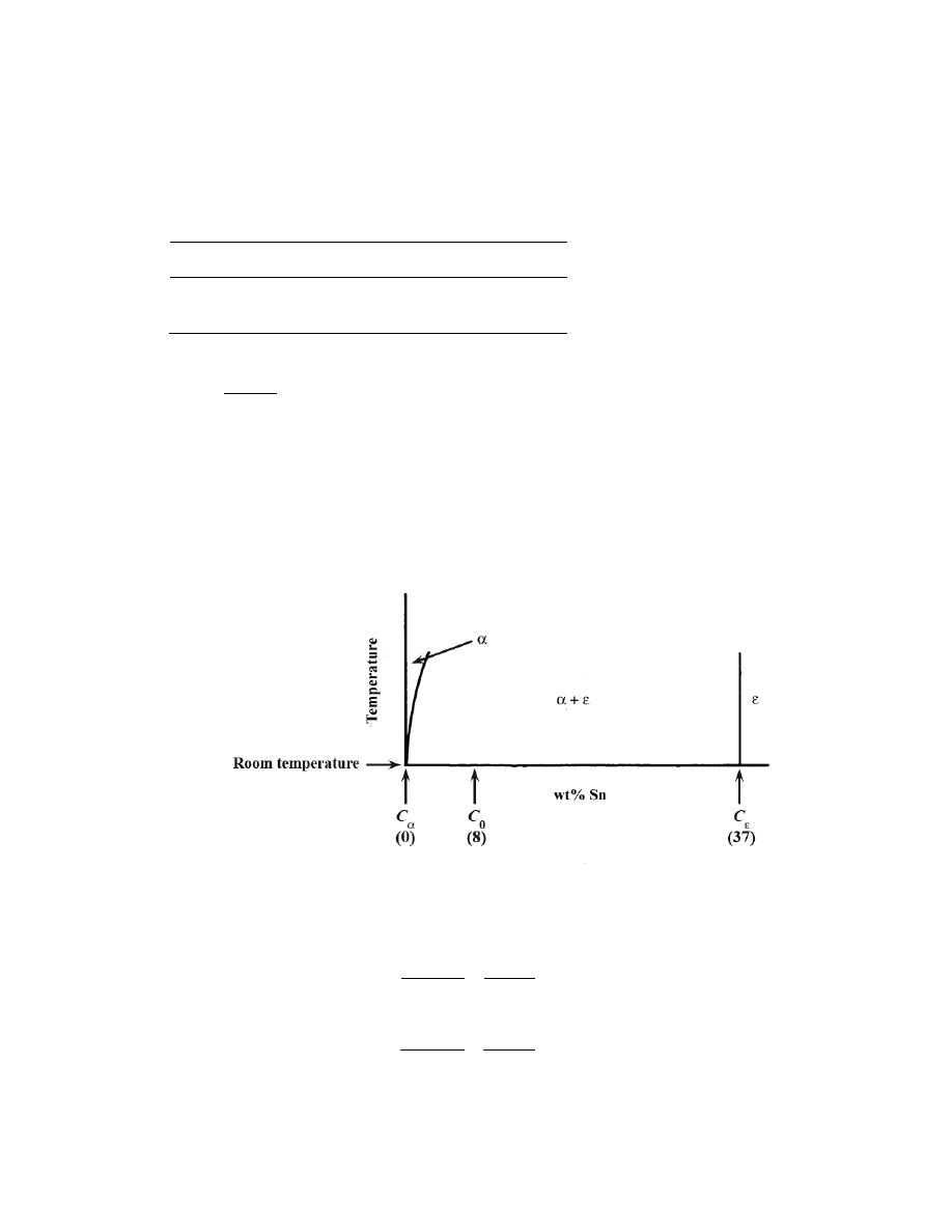
Excerpts from this work may be reproduced by instructors for distribution on a not-for-profit basis for testing or instructional purposes only to
students enrolled in courses for which the textbook has been adopted. Any other reproduction or translation of this work beyond that permitted
by Sections 107 or 108 of the 1976 United States Copyright Act without the permission of the copyright owner is unlawful.
18.16 Tin bronze has a composition of 92 wt% Cu and 8 wt% Sn, and consists of two phases at room
temperature: an
α phase, which is copper containing a very small amount of tin in solid solution, and an ε phase,
which consists of approximately 37 wt% Sn. Compute the room temperature conductivity of this alloy given the
following data:
Phase
Electrical Resistivity
(Ω-m)
Density (g/cm
3
)
α
1.88 × 10
–8
8.94
ε
5.32 × 10
–7
8.25
Solution
This problem asks for us to compute the room-temperature conductivity of a two-phase Cu-Sn alloy which
composition is 92 wt% Cu-8 wt% Sn. It is first necessary for us to determine the volume fractions of the
α and ε
phases, after which the resistivity (and subsequently, the conductivity) may be calculated using Equation 18.12.
Weight fractions of the two phases are first calculated using the phase diagram information provided in the problem.
We may represent a portion of the phase diagram near room temperature as follows:
Applying the lever rule to this situation
W
α
=
Cε − C
0
Cε − C
α
=
37
− 8
37
− 0
= 0.784
Wε =
C
0
− C
α
Cε − C
α
=
8
− 0
37
− 0
= 0.216
Excerpts from this work may be reproduced by instructors for distribution on a not-for-profit basis for testing or instructional purposes only to
students enrolled in courses for which the textbook has been adopted. Any other reproduction or translation of this work beyond that permitted
by Sections 107 or 108 of the 1976 United States Copyright Act without the permission of the copyright owner is unlawful.
We must now convert these mass fractions into volume fractions using the phase densities given in the problem
statement. (Note: in the following expressions, density is represented by
ρ' in order to avoid confusion with
resistivity which is designated by
ρ.) Utilization of Equations 9.6a and 9.6b leads to
V
α
=
W
α
ρ'
α
W
α
ρ'
α
+
Wε
ρ'ε
=
0.784
8.94 g/cm
3
0.784
8.94 g/cm
3
+
0.216
8.25 g/cm
3
= 0.770
Vε =
Wε
ρ'ε
W
α
ρ'
α
+
Wε
ρ'ε
=
0.216
8.25 g/cm
3
0.784
8.94 g/cm
3
+
0.216
8.25 g/cm
3
= 0.230
Now, using Equation 18.12
ρ = ρ
α
V
α
+
ρεVε
=
(
1.88
× 10
-8
Ω - m
)
(0.770) +
(
5.32
× 10
-7
Ω - m
)
(0.230)
= 1.368
× 10
-7
Ω-m

Excerpts from this work may be reproduced by instructors for distribution on a not-for-profit basis for testing or instructional purposes only to
students enrolled in courses for which the textbook has been adopted. Any other reproduction or translation of this work beyond that permitted
by Sections 107 or 108 of the 1976 United States Copyright Act without the permission of the copyright owner is unlawful.
Finally, for the conductivity (Equation 18.4)
σ =
1
ρ
=
1
1.368
× 10
−7
Ω − m
= 7.31
× 10
6
(
Ω - m)
-1

Excerpts from this work may be reproduced by instructors for distribution on a not-for-profit basis for testing or instructional purposes only to
students enrolled in courses for which the textbook has been adopted. Any other reproduction or translation of this work beyond that permitted
by Sections 107 or 108 of the 1976 United States Copyright Act without the permission of the copyright owner is unlawful.
18.17 A cylindrical metal wire 2 mm (0.08 in.) in diameter is required to carry a current of 10 A with a
minimum of 0.03 V drop per foot (300 mm) of wire. Which of the metals and alloys listed in Table 18.1 are possible
candidates?
Solution
We are asked to select which of several metals may be used for a 2 mm diameter wire to carry 10 A, and
have a voltage drop less than 0.03 V per foot (300 mm). Using Equations 18.3 and 18.4, let us determine the
minimum conductivity required, and then select from Table 18.1, those metals that have conductivities greater than
this value. Combining Equations 18.3 and 18.4, the minimum conductivity is just
σ =
1
ρ
=
Il
VA
=
Il
V
π
d
2
2
=
(10 A)
(
300
× 10
−3
m
)
(0.03 V) (
π)
2
× 10
−3
m
2
2
= 3.2
× 10
7
(
Ω - m)
-1
Thus, from Table 18.1, only aluminum, gold, copper, and silver are candidates.

Excerpts from this work may be reproduced by instructors for distribution on a not-for-profit basis for testing or instructional purposes only to
students enrolled in courses for which the textbook has been adopted. Any other reproduction or translation of this work beyond that permitted
by Sections 107 or 108 of the 1976 United States Copyright Act without the permission of the copyright owner is unlawful.
Intrinsic Semiconduction
18.18 (a) Using the data presented in Figure 18.16, determine the number of free electrons per atom for
intrinsic germanium and silicon at room temperature (298 K). The densities for Ge and Si are 5.32 and 2.33 g/cm
3
,
respectively.
(b) Now explain the difference in these free-electron-per-atom values.
Solution
(a) For this part of the problem, we first read, from Figure 18.16, the number of free electrons (i.e., the
intrinsic carrier concentration) at room temperature (298 K). These values are n
i
(Ge) = 5
× 10
19
m
-3
and n
i
(Si) = 7
× 10
16
m
-3
.
Now, the number of atoms per cubic meter for Ge and Si (N
Ge
and N
Si
, respectively) may be determined
using Equation 4.2 which involves the densities (
ρ
Ge
'
and
ρ
Si
'
) and atomic weights (A
Ge
and A
Si
). (Note: here we
use
ρ' to represent density in order to avoid confusion with resistivity, which is designated by ρ. Also, the atomic
weights for Ge and Si, 72.64 and 28.09 g/mol, respectively, are found inside the front cover.) Therefore,
N
Ge
=
N
A
ρ
Ge
'
A
Ge
=
(
6.022
× 10
23
atoms/mol
)(
5.32 g/cm
3
)(
10
6
cm
3
/m
3
)
72.64 g/mol
= 4.41
× 10
28
atoms/m
3
Similarly, for Si
N
Si
=
N
A
ρ
Si
'
A
Si
=
(
6.022
× 10
23
atoms / mol
)(
2.33 g/cm
3
)(
10
6
cm
3
/m
3
)
28.09 g/mol
= 5.00
× 10
28
atoms/m
3
Finally, the ratio of the number of free electrons per atom is calculated by dividing n
i
by N. For Ge

Excerpts from this work may be reproduced by instructors for distribution on a not-for-profit basis for testing or instructional purposes only to
students enrolled in courses for which the textbook has been adopted. Any other reproduction or translation of this work beyond that permitted
by Sections 107 or 108 of the 1976 United States Copyright Act without the permission of the copyright owner is unlawful.
n
i
(Ge)
N
Ge
=
5
× 10
19
electrons / m
3
4.41
× 10
28
atoms / m
3
1.13
× 10
-9
electron/atom
And, for Si
n
i(Si)
N
Si
=
7
× 10
16
electrons / m
3
5.00
× 10
28
atoms / m
3
= 1.40
× 10
-12
electron/atom
(b) The difference is due to the magnitudes of the band gap energies (Table 18.3). The band gap energy at
room temperature for Si (1.11 eV) is larger than for Ge (0.67 eV), and, consequently, the probability of excitation
across the band gap for a valence electron is much smaller for Si.
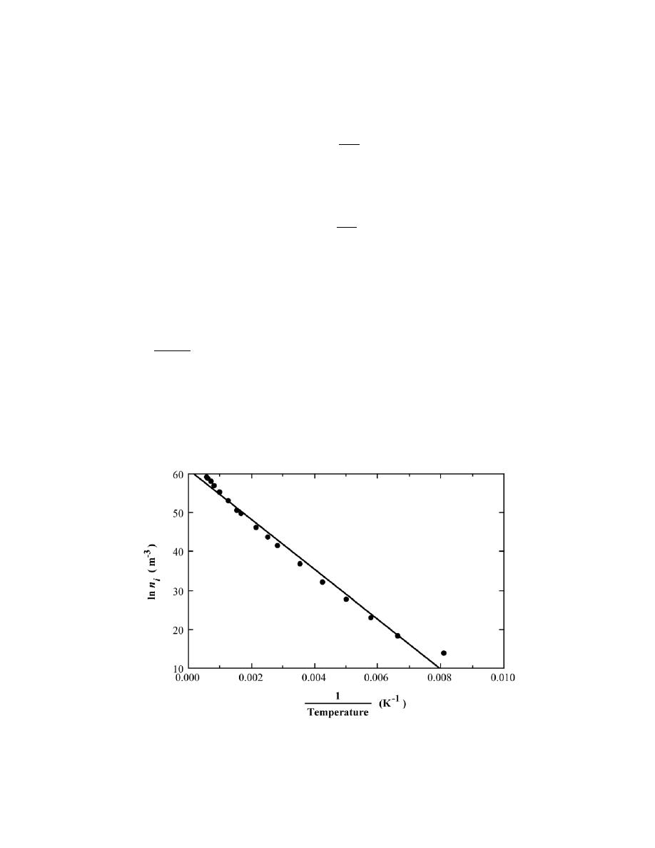
Excerpts from this work may be reproduced by instructors for distribution on a not-for-profit basis for testing or instructional purposes only to
students enrolled in courses for which the textbook has been adopted. Any other reproduction or translation of this work beyond that permitted
by Sections 107 or 108 of the 1976 United States Copyright Act without the permission of the copyright owner is unlawful.
18.19 For intrinsic semiconductors, the intrinsic carrier concentration n
i
depends on temperature as
follows:
n
i
∝ exp −
E
g
2kT
(18.35a)
or taking natural logarithms,
ln n
i
∝ −
E
g
2kT
(18.35b)
Thus, a plot of ln n
i
versus 1/T (K)
–1
should be linear and yield a slope of –E
g
/2k. Using this information and the
data presented in Figure 18.16, determine the band gap energies for silicon and germanium, and compare these
values with those given in Table 18.3.
Solution
This problem asks that we make plots of ln n
i
versus reciprocal temperature for both Si and Ge, using the
data presented in Figure 18.16, and then determine the band gap energy for each material realizing that the slope of
the resulting line is equal to – E
g
/2k.
Below is shown such a plot for Si.
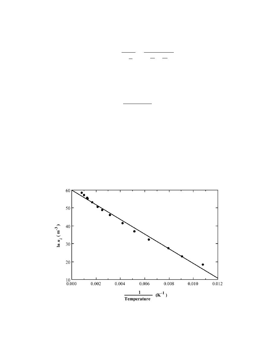
Excerpts from this work may be reproduced by instructors for distribution on a not-for-profit basis for testing or instructional purposes only to
students enrolled in courses for which the textbook has been adopted. Any other reproduction or translation of this work beyond that permitted
by Sections 107 or 108 of the 1976 United States Copyright Act without the permission of the copyright owner is unlawful.
The slope of the line is equal to
Slope =
∆ ln η
i
∆
1
T
=
ln
η
1
− ln η
2
1
T
1
−
1
T
2
Let us take 1/T
1
= 0.001 and 1/T
2
= 0.007; their corresponding ln
η values are ln η
1
= 54.80 and ln
η
2
= 16.00.
Incorporating these values into the above expression leads to a slope of
Slope =
54.80
− 16.00
0.001
− 0.007
= − 6467
This slope leads to an E
g
value of
E
g
= – 2k (Slope)
= − 2
(
8.62 x 10
−5
eV / K
)
(
− 6467) = 1.115 eV
The value cited in Table 18.3 is 1.11 eV.
Now for Ge, an analogous plot is shown below.

Excerpts from this work may be reproduced by instructors for distribution on a not-for-profit basis for testing or instructional purposes only to
students enrolled in courses for which the textbook has been adopted. Any other reproduction or translation of this work beyond that permitted
by Sections 107 or 108 of the 1976 United States Copyright Act without the permission of the copyright owner is unlawful.
We calculate the slope and band gap energy values in the manner outlined above. Let us take 1/T
1
= 0.001 and 1/T
2
= 0.011; their corresponding ln
η values are ln η
1
= 55.56 and ln
η
2
= 14.80. Incorporating these values into the
above expression leads to a slope of
Slope =
55.56ÊÊ
− 14.80
0.001
− 0.011
= − 4076
This slope leads to an E
g
value of
E
g
= – 2k (Slope)
= − 2
(
8.62
× 10
−5
eV / K
)
(
− 4076) = 0.70 eV
This value is in good agreement with the 0.67 eV cited in Table 18.3.

Excerpts from this work may be reproduced by instructors for distribution on a not-for-profit basis for testing or instructional purposes only to
students enrolled in courses for which the textbook has been adopted. Any other reproduction or translation of this work beyond that permitted
by Sections 107 or 108 of the 1976 United States Copyright Act without the permission of the copyright owner is unlawful.
18.20 Briefly explain the presence of the factor 2 in the denominator of Equation 18.35a.
Solution
The factor 2 in Equation 18.35a takes into account the creation of two charge carriers (an electron and a
hole) for each valence-band-to-conduction-band intrinsic excitation; both charge carriers may participate in the
conduction process.

Excerpts from this work may be reproduced by instructors for distribution on a not-for-profit basis for testing or instructional purposes only to
students enrolled in courses for which the textbook has been adopted. Any other reproduction or translation of this work beyond that permitted
by Sections 107 or 108 of the 1976 United States Copyright Act without the permission of the copyright owner is unlawful.
18.21
At room temperature the electrical conductivity of PbTe is 500 (Ω-m)
–1
, whereas the electron and
hole mobilities are 0.16 and 0.075 m
2
/V-s, respectively. Compute the intrinsic carrier concentration for PbTe at
room temperature.
Solution
In this problem we are asked to compute the intrinsic carrier concentration for PbTe at room temperature.
Since the conductivity and both electron and hole mobilities are provided in the problem statement, all we need do
is solve for n and p (i.e., n
i
) using Equation 18.15. Thus,
n
i
=
σ
| e |
(
µ
e
+ µ
h
)
=
500 (
Ω - m)
−1
(
1.602
× 10
−19
C
)(
0.16
+ 0.075
)
m
2
/V - s
= 1.33
× 10
22
m
-3

Excerpts from this work may be reproduced by instructors for distribution on a not-for-profit basis for testing or instructional purposes only to
students enrolled in courses for which the textbook has been adopted. Any other reproduction or translation of this work beyond that permitted
by Sections 107 or 108 of the 1976 United States Copyright Act without the permission of the copyright owner is unlawful.
18.22 Is it possible for compound semiconductors to exhibit intrinsic behavior? Explain your answer.
Solution
Yes, compound semiconductors can exhibit intrinsic behavior. They will be intrinsic even though they are
composed of two different elements as long as the electrical behavior is not influenced by the presence of other
elements.

Excerpts from this work may be reproduced by instructors for distribution on a not-for-profit basis for testing or instructional purposes only to
students enrolled in courses for which the textbook has been adopted. Any other reproduction or translation of this work beyond that permitted
by Sections 107 or 108 of the 1976 United States Copyright Act without the permission of the copyright owner is unlawful.
18.23 For each of the following pairs of semiconductors, decide which will have the smaller band gap
energy, E
g,
and then cite the reason for your choice. (a) ZnS and CdSe, (b) Si and C (diamond), (c) Al
2
O
3
and
ZnTe, (d) InSb and ZnSe, and (e) GaAs and AlP.
Solution
This problem calls for us to decide for each of several pairs of semiconductors, which will have the smaller
band gap energy and then cite a reason for the choice.
(a) Cadmium selenide will have a smaller band gap energy than zinc sulfide. Both are II-VI compounds,
and Cd and Se are both lower vertically in the periodic table (Figure 2.6) than Zn and S. In moving from top to
bottom down the periodic table, E
g
decreases.
(b) Silicon will have a smaller band gap energy than diamond since Si is lower in column IVA of the
periodic table than is C.
(c) Zinc telluride will have a smaller band gap energy that aluminum oxide. There is a greater disparity
between the electronegativities for aluminum and oxygen [1.5 versus 3.5 (Figure 2.7)] than for zinc and tellurium
(1.6 and 2.1). For binary compounds, the larger the difference between the electronegativities of the elements, the
greater the band gap energy.
(d) Indium antimonide will have a smaller band gap energy than zinc selenide. These materials are III-V
and II-VI compounds, respectively; Thus, in the periodic table, In and Sb are closer together horizontally than are
Zn and Se. Furthermore, both In and Sb reside below Zn and Se in the periodic table.
(e) Gallium arsenide will have a smaller band gap energy than aluminum phosphide. Both are III-V
compounds, and Ga and As are both lower vertically in the periodic table than Al and P.

Excerpts from this work may be reproduced by instructors for distribution on a not-for-profit basis for testing or instructional purposes only to
students enrolled in courses for which the textbook has been adopted. Any other reproduction or translation of this work beyond that permitted
by Sections 107 or 108 of the 1976 United States Copyright Act without the permission of the copyright owner is unlawful.
Extrinsic Semiconduction
18.24 Define the following terms as they pertain to semiconducting materials: intrinsic, extrinsic,
compound, elemental. Now provide an example of each.
Solution
These semiconductor terms are defined in the Glossary. Examples are as follows: intrinsic--high purity
(undoped) Si, GaAs, CdS, etc.; extrinsic--P-doped Ge, B-doped Si, S-doped GaP, etc.; compound--GaAs, InP, CdS,
etc.; elemental--Ge and Si.

Excerpts from this work may be reproduced by instructors for distribution on a not-for-profit basis for testing or instructional purposes only to
students enrolled in courses for which the textbook has been adopted. Any other reproduction or translation of this work beyond that permitted
by Sections 107 or 108 of the 1976 United States Copyright Act without the permission of the copyright owner is unlawful.
18.25 An n-type semiconductor is known to have an electron concentration of 3
× 10
18
m
-3
. If the electron
drift velocity is 100 m/s in an electric field of 500 V/m, calculate the conductivity of this material.
Solution
The conductivity of this material may be computed using Equation 18.16. But before this is possible, it is
necessary to calculate the value of
µ
e
from Equation 18.7. Thus, the electron mobility is equal to
µ
e
=
v
d
E
=
100 m/s
500 V/m
= 0.20 m
2
/V
− s
Thus, from Equation 18.16, the conductivity is
σ = n| e |µ
e
=
(
3
× 10
18
m
−3
)(
1.602
× 10
−19
C
)(
0.20 m
2
/V
− s
)
= 0.096 (
Ω-m)
-1

Excerpts from this work may be reproduced by instructors for distribution on a not-for-profit basis for testing or instructional purposes only to
students enrolled in courses for which the textbook has been adopted. Any other reproduction or translation of this work beyond that permitted
by Sections 107 or 108 of the 1976 United States Copyright Act without the permission of the copyright owner is unlawful.
18.26 (a) In your own words, explain how donor impurities in semiconductors give rise to free electrons in
numbers in excess of those generated by valence band–conduction band excitations. (b) Also explain how acceptor
impurities give rise to holes in numbers in excess of those generated by valence band–conduction band excitations.
The explanations called for are found in Section 18.11.

Excerpts from this work may be reproduced by instructors for distribution on a not-for-profit basis for testing or instructional purposes only to
students enrolled in courses for which the textbook has been adopted. Any other reproduction or translation of this work beyond that permitted
by Sections 107 or 108 of the 1976 United States Copyright Act without the permission of the copyright owner is unlawful.
18.27 (a) Explain why no hole is generated by the electron excitation involving a donor impurity atom. (b)
Explain why no free electron is generated by the electron excitation involving an acceptor impurity atom.
Solution
(a) No hole is generated by an electron excitation involving a donor impurity atom because the excitation
comes from a level within the band gap, and thus, no missing electron is created within the normally filled valence
band.
(b) No free electron is generated by an electron excitation involving an acceptor impurity atom because the
electron is excited from the valence band into the impurity level within the band gap; no free electron is introduced
into the conduction band.

Excerpts from this work may be reproduced by instructors for distribution on a not-for-profit basis for testing or instructional purposes only to
students enrolled in courses for which the textbook has been adopted. Any other reproduction or translation of this work beyond that permitted
by Sections 107 or 108 of the 1976 United States Copyright Act without the permission of the copyright owner is unlawful.
18.28 Will each of the following elements act as a donor or an acceptor when added to the indicated
semiconducting material? Assume that the impurity elements are substitutional.
Impurity
Semiconductor
P
Ge
S
AlP
In
CdTe
Al
Si
Cd
GaAs
Sb
ZnSe
Solution
Phosphorus will act as a donor in Ge. Since it (P) is from group VA of the periodic table (Figure 2.6), a P
atom has one more valence electron than a Ge atom.
Sulfur will act as a donor in AlP. Since S is from group VIA of the periodic table, it will substitute for P;
also, an S atom has one more valence electron than a P atom.
Indium will act as a donor in CdTe. Since In is from group IIIA of the periodic table, it will substitute for
Cd; furthermore, an In atom has one more valence electron than a Cd atom.
Aluminum will act as an acceptor in Si. Since it (Al) is from group IIIA of the periodic table (Figure 2.6),
an Al atom has one less valence electron than a Si atom.
Cadmium will act as an acceptor in GaAs. Since Cd is from group IIB of the periodic table, it will
substitute for Ga; furthermore, a Cd atom has one less valence electron than a Ga atom.
Antimony will act as an acceptor in ZnSe. Since Sb is from group VA of the periodic table, it will
substitute for Se; and, an Sb atom has one less valence electron than an Se atom.

Excerpts from this work may be reproduced by instructors for distribution on a not-for-profit basis for testing or instructional purposes only to
students enrolled in courses for which the textbook has been adopted. Any other reproduction or translation of this work beyond that permitted
by Sections 107 or 108 of the 1976 United States Copyright Act without the permission of the copyright owner is unlawful.
18.29 (a) The room-temperature electrical conductivity of a silicon specimen is 5.93
× 10
–3
(Ω-m)
–1
. The
hole concentration is known to be 7.0
× 10
17
m
–3
. Using the electron and hole mobilities for silicon in Table 18.3,
compute the electron concentration. (b) On the basis of the result in part (a), is the specimen intrinsic, n-type
extrinsic, or p-type extrinsic? Why?
Solution
(a) In this problem, for a Si specimen, we are given values for p
(
7.0
× 10
17
m
-3
)
and
σ
[
5.93 × 10
-3
(
Ω-
m)
-1
]
, while values for
µ
h
and
µ
e
(0.05 and 0.14 m
2
/V-s, respectively) are found in Table 18.3. In order to solve
for n we must use Equation 18.13, which, after rearrangement, leads to
n =
σ − p| e | µ
h
| e |
µ
e
=
5.93
× 10
−3
(
Ω − m)
−1
−
(
7.0
× 10
17
m
−3
)(
1.602
× 10
−19
C
)(
0.05 m
2
/ V - s
)
(
1.602
× 10
−19
C
)(
0.14 m
2
/ V - s
)
= 1.44
× 10
16
m
-3
(b) This material is p-type extrinsic since p
(
7.0
× 10
17
m
-3
)
is greater than n
(
1.44
× 10
16
m
-3
)
.

Excerpts from this work may be reproduced by instructors for distribution on a not-for-profit basis for testing or instructional purposes only to
students enrolled in courses for which the textbook has been adopted. Any other reproduction or translation of this work beyond that permitted
by Sections 107 or 108 of the 1976 United States Copyright Act without the permission of the copyright owner is unlawful.
18.30 Germanium to which 5
× 10
22
m
-3
Sb atoms have been added is an extrinsic semiconductor at room
temperature, and virtually all the Sb atoms may be thought of as being ionized (i.e., one charge carrier exists for
each Sb atom). (a) Is this material n-type or p-type? (b) Calculate the electrical conductivity of this material,
assuming electron and hole mobilities of 0.1 and 0.05 m
2
/V-s, respectively.
Solution
(a) (a) This germanium material to which has been added 5
× 10
22
m
-3
Sb atoms is n-type since Sb is a
donor in Ge. (Antimony is from group VA of the periodic table--Ge is from group IVA.)
(b) Since this material is n-type extrinsic, Equation 18.16 is valid. Furthermore, each Sb will donate a
single electron, or the electron concentration is equal to the Sb concentration since all of the Sb atoms are ionized at
room temperature; that is n = 5
× 10
22
m
-3
, and, as given in the problem statement,
µ
e
= 0.1 m
2
/V-s. Thus
σ = n| e |µ
e
=
(
5
× 10
22
m
-3
)(
1.602
× 10
-19
C
)(
0.1 m
2
/V - s
)
= 800 (
Ω-m)
-1

Excerpts from this work may be reproduced by instructors for distribution on a not-for-profit basis for testing or instructional purposes only to
students enrolled in courses for which the textbook has been adopted. Any other reproduction or translation of this work beyond that permitted
by Sections 107 or 108 of the 1976 United States Copyright Act without the permission of the copyright owner is unlawful.
18.31 The following electrical characteristics have been determined for both intrinsic and p-type extrinsic
indium phosphide (InP) at room temperature:
σ (Ω -m)
–1
n (m
–3
)
p (m
–3
)
Intrinsic
2.5 × 10
-6
3.0 × 10
13
3.0 × 10
13
Extrinsic (n-type)
3.6 × 10
-5
4.5 × 10
14
2.0 × 10
12
Calculate electron and hole mobilities.
Solution
In order to solve for the electron and hole mobilities for InP, we must write conductivity expressions for
the two materials, of the form of Equation 18.13—i.e.,
σ = n| e | µ
e
+ p | e |
µ
h
For the intrinsic material
2.5
× 10
-6
(
Ω - m)
-1
=
(
3.0
× 10
13
m
-3
)(
1.602
× 10
-19
C
)
µ
e
+ (
3.0
× 10
13
m
-3
)(
1.602
× 10
-19
C
)
µ
h
which reduces to
0.52 =
µ
e
+
µ
h
Whereas, for the extrinsic InP
3.6
× 10
-5
(
Ω - m)
-1
=
(
4.5
× 10
14
m
-3
)(
1.602
× 10
-19
C
)
µ
e
+
(
2.0
× 10
12
m
-3
)(
1.602
× 10
-19
C
)
µ
h
which may be simplified to
112.4 = 225
µ
e
+
µ
h
Thus, we have two independent expressions with two unknown mobilities. Upon solving these equations
simultaneously, we get
µ
e
= 0.50 m
2
/V-s and
µ
h
= 0.02 m
2
/V-s.

Excerpts from this work may be reproduced by instructors for distribution on a not-for-profit basis for testing or instructional purposes only to
students enrolled in courses for which the textbook has been adopted. Any other reproduction or translation of this work beyond that permitted
by Sections 107 or 108 of the 1976 United States Copyright Act without the permission of the copyright owner is unlawful.
The Temperature Dependence of Carrier Concentration
18.32 Calculate the conductivity of intrinsic silicon at 100°C.
Solution
In order to estimate the electrical conductivity of intrinsic silicon at 100
°C, we must employ Equation
18.15. However, before this is possible, it is necessary to determine values for n
i
,
µ
e
, and
µ
h
. According to Figure
18.16, at 100
°C (373 K), n
i
= 2
× 10
18
m
-3
, whereas from the "<10
20
m
-3
" curves of Figures 18.19a and 18.19b, at
100ºC (373 K),
µ
e
= 0.09 m
2
/V-s and
µ
h
= 0.032 m
2
/V-s (realizing that the mobility axes of these two plot are
scaled logarithmically). Thus, the conductivity at 100
°C is
σ = n
i
| e |
(
µ
e
+
µ
h
)
σ =
(
2
× 10
18
m
−3
)(
1.602
× 10
−19
C
)(
0.09 m
2
/V - s + 0.032 m
2
/ V
− s
)
= 0.039 (Ω - m)
-1

Excerpts from this work may be reproduced by instructors for distribution on a not-for-profit basis for testing or instructional purposes only to
students enrolled in courses for which the textbook has been adopted. Any other reproduction or translation of this work beyond that permitted
by Sections 107 or 108 of the 1976 United States Copyright Act without the permission of the copyright owner is unlawful.
18.33 At temperatures near room temperature, the temperature dependence of the conductivity for
intrinsic germanium is found to equal
σ = CT
−3/ 2
exp
−
E
g
2kT
(18.36)
where C is a temperature-independent constant and T is in Kelvins. Using Equation 18.36, calculate the intrinsic
electrical conductivity of germanium at 150°C.
Solution
It first becomes necessary to solve for C in Equation 18.36 using the room-temperature (298 K)
conductivity [2.2 (
Ω-m)
-1
] (Table 18.3). This is accomplished by taking natural logarithms of both sides of
Equation 18.36 as
ln
σ = ln C −
3
2
ln T
−
E
g
2 kT
and after rearranging and substitution of values for E
g
(0.67 eV, Table 18.3), and the room-temperature
conductivity, we get
ln C = ln
σ +
3
2
ln T +
E
g
2 kT
= ln (2.2) +
3
2
ln (298) +
0.67 eV
(2)
(
8.62
× 10
−5
eV / K
)
(298 K)
= 22.38
Now, again using Equation 18.36, we are able to compute the conductivity at 423 K (150
°C)
ln
σ = ln C −
3
2
ln T
−
E
g
2 kT
= 22.38
−
3
2
ln (423 K)
−
0.67 eV
(2)
(
8.62
× 10
−5
eV / K
)
(423 K)
= 4.12

Excerpts from this work may be reproduced by instructors for distribution on a not-for-profit basis for testing or instructional purposes only to
students enrolled in courses for which the textbook has been adopted. Any other reproduction or translation of this work beyond that permitted
by Sections 107 or 108 of the 1976 United States Copyright Act without the permission of the copyright owner is unlawful.
which leads to
σ = e
4.12
= 61.6 (
Ω-m)
-1
.

Excerpts from this work may be reproduced by instructors for distribution on a not-for-profit basis for testing or instructional purposes only to
students enrolled in courses for which the textbook has been adopted. Any other reproduction or translation of this work beyond that permitted
by Sections 107 or 108 of the 1976 United States Copyright Act without the permission of the copyright owner is unlawful.
18.34 Using Equation 18.36 and the results of Problem 18.33, determine the temperature at which the
electrical conductivity of intrinsic germanium is 22.8 (Ω-m)
–1
.
Solution
This problem asks that we determine the temperature at which the electrical conductivity of intrinsic Ge is
22.8 (
Ω-m)
-1
, using Equation 18.36 and the results of Problem 18.33. First of all, taking logarithms of Equation
18.36
ln
σ = ln C −
3
2
ln T
−
E
g
2 kT
And, from Problem 18.33 the value of ln C was determined to be 22.38. Using this and
σ = 22.8 (Ω-m)
-1
, the above
equation takes the form
ln 22.8
= 22.38 −
3
2
ln T
−
0.67 eV
(2)
(
8.62
× 10
−5
eV / K
)
(T)
In order to solve for T from the above expression it is necessary to use an equation solver. For some solvers, the
following set of instructions may be used:
ln(22.8) = 22.38 –1.5*ln(T) – 0.67/(2*8.62*10^-5*T)
The resulting solution is T = 375, which value is the temperature in K; this corresponds to T(ºC) = 375 – 273 =
102
°C.

Excerpts from this work may be reproduced by instructors for distribution on a not-for-profit basis for testing or instructional purposes only to
students enrolled in courses for which the textbook has been adopted. Any other reproduction or translation of this work beyond that permitted
by Sections 107 or 108 of the 1976 United States Copyright Act without the permission of the copyright owner is unlawful.
18.35 Estimate the temperature at which GaAs has an electrical conductivity of 3.7 3 10
2
3
(V-m)
2
1
assuming the temperature dependence for
σ of Equation 18.36. The data shown in Table 18.3 might prove helpful.
Solution
This problem asks that we estimate the temperature at which GaAs has an electrical conductivity of 3.7
×
10
-3
(
Ω-m)
-1
assuming that the conductivity has a temperature dependence as shown in Equation 18.36. From the
room temperature (298 K) conductivity [10
-6
(
Ω-m)
-1
] and band gap energy (1.42 eV) of Table 18.3 we determine
the value of C (Equation 18.36) by taking natural logarithms of both sides of the equation, and after rearrangement
as follows:
ln C = ln
σ +
3
2
ln T +
E
g
2 kT
= ln 10
−6
(
Ω − m)
−1
[
]
+
3
2
ln (298 K) +
1.42 eV
(2)
(
8.62
× 10
−5
eV / K
)
(298 K)
= 22.37
Now we substitute this value into Equation 18.36 in order to determine the value of T for which
σ = 3.7 × 10
-3
(
Ω-
m)
-1
, thus
ln
σ = ln C −
3
2
ln T
−
E
g
2 kT
ln 3.7
× 10
-3
(
Ω - m)
-1
[
]
= 22.37
−
3
2
ln T
−
1.42 eV
(2)
(
8.62
× 10
−5
eV / K
)
(T)
This equation may be solved for T using an equation solver. For some solvers, the following set of instructions may
be used:
ln(3.7*10^–3) = 22.37 – 1.5*ln(T) – 1.42/(2*8.62*10^–5*T)
The resulting solution is T = 437; this value is the temperature in K which corresponds to T(ºC) = 437 K – 273 =
164
°C.

Excerpts from this work may be reproduced by instructors for distribution on a not-for-profit basis for testing or instructional purposes only to
students enrolled in courses for which the textbook has been adopted. Any other reproduction or translation of this work beyond that permitted
by Sections 107 or 108 of the 1976 United States Copyright Act without the permission of the copyright owner is unlawful.
18.36 Compare the temperature dependence of the conductivity for metals and intrinsic semiconductors.
Briefly explain the difference in behavior.
Solution
For metals, the temperature dependence is described by Equation 18.10 (and converting from resistivity to
conductivity using Equation 18.4), as
σ =
1
ρ
0
+ aT
That is, the electrical conductivity decreases with increasing temperature.
Alternatively, from Equation 18.8, the conductivity of metals is equal to
σ = n| e |µ
e
As the temperature rises, n will remain virtually constant, whereas the mobility (
µ
e
) will decrease, because the
thermal scattering of free electrons will become more efficient. Since |e| is independent of temperature, the net
result will be diminishment in the magnitude of
σ.
For intrinsic semiconductors, the temperature-dependence of conductivity is just the opposite of that for
metals—i.e, conductivity increases with rising temperature. One explanation is as follows: Equation 18.15
describes the conductivity; i.e.,
σ = n| e |
(
µ
e
+
µ
h
)
= p | e |
(
µ
e
+
µ
h
)
= n
i
| e |
(
µ
e
+
µ
h
)
Both n and p increase dramatically with rising temperature (Figure 18.16), since more thermal energy becomes
available for valence band-conduction band electron excitations. The magnitudes of
µ
e
and
µ
h
will diminish
somewhat with increasing temperature (per the upper curves of Figures 18.19a and 18.19b), as a consequence of the
thermal scattering of electrons and holes. However, this reduction of
µ
e
and
µ
h
will be overwhelmed by the
increase in n and p, with the net result is that
σ increases with temperature.
An alternative explanation is as follows: for an intrinsic semiconductor the temperature dependence is
represented by an equation of the form of Equation 18.36. This expression contains two terms that involve
temperature—a preexponential one (in this case T
-3/2
) and the other in the exponential. With rising temperature the
preexponential term decreases, while the exp (–E
g
/2kT) parameter increases. With regard to relative magnitudes,

Excerpts from this work may be reproduced by instructors for distribution on a not-for-profit basis for testing or instructional purposes only to
students enrolled in courses for which the textbook has been adopted. Any other reproduction or translation of this work beyond that permitted
by Sections 107 or 108 of the 1976 United States Copyright Act without the permission of the copyright owner is unlawful.
the exponential term increases much more rapidly than the preexponential one, such that the electrical conductivity
of an intrinsic semiconductor increases with rising temperature.

Excerpts from this work may be reproduced by instructors for distribution on a not-for-profit basis for testing or instructional purposes only to
students enrolled in courses for which the textbook has been adopted. Any other reproduction or translation of this work beyond that permitted
by Sections 107 or 108 of the 1976 United States Copyright Act without the permission of the copyright owner is unlawful.
Factors That Affect Carrier Mobility
18.37 Calculate the room-temperature electrical conductivity of silicon that has been doped with 5
× 10
22
m
–3
of boron atoms.
Solution
This problems asks that we determine the room-temperature electrical conductivity of silicon that has been
doped with 5
× 10
22
m
-3
of boron atoms. Inasmuch as B is a group IIIA element in the periodic table (Figure 2.6) it
acts as an acceptor in silicon. Thus, this material is p-type extrinsic, and it is necessary to use Equation 18.17, with
p = 5
× 10
22
m
-3
since at room temperature all of the B acceptor impurities are ionized. The hole mobility, from
Figure 18.18 at an impurity concentration of 5
× 10
22
m
-3
, is 0.028 m
2
/V-s. Therefore, the conductivity is equal to
σ = p | e | µ
h
=
(
5
× 10
22
m
−3
)(
1.602
× 10
−19
C
)(
0.028 m
2
/ V
− s
)
= 224 (Ω − m)
−1

Excerpts from this work may be reproduced by instructors for distribution on a not-for-profit basis for testing or instructional purposes only to
students enrolled in courses for which the textbook has been adopted. Any other reproduction or translation of this work beyond that permitted
by Sections 107 or 108 of the 1976 United States Copyright Act without the permission of the copyright owner is unlawful.
18.38 Calculate the room-temperature electrical conductivity of silicon that has been doped with 2 × 10
23
m
–3
of arsenic atoms.
Solution
Here we are asked to calculate the room-temperature electrical conductivity of silicon that has been doped
with 2
× 10
23
m
-3
of arsenic atoms. Inasmuch as As is a group VA element in the periodic table (Figure 2.6) it acts
as a donor in silicon. Thus, this material is n-type extrinsic, and it is necessary to use Equation 18.16, with n = 2
×
10
23
m
-3
since at room temperature all of the As donor impurities are ionized. The electron mobility, from Figure
18.18 at an impurity concentration of 2
× 10
23
m
-3
, is 0.05 m
2
/V-s. Therefore, the conductivity is equal to
σ = n | e | µ
e
=
(
2
× 10
23
m
−3
)(
1.602
× 10
−19
C
)(
0.05 m
2
/ V
− s
)
= 1600 (Ω − m)
−1

Excerpts from this work may be reproduced by instructors for distribution on a not-for-profit basis for testing or instructional purposes only to
students enrolled in courses for which the textbook has been adopted. Any other reproduction or translation of this work beyond that permitted
by Sections 107 or 108 of the 1976 United States Copyright Act without the permission of the copyright owner is unlawful.
18.39 Estimate the electrical conductivity, at 125°C, of silicon that has been doped with 10
23
m
–3
of
aluminum atoms.
Solution
In this problem we are to estimate the electrical conductivity, at 125
°C, of silicon that has been doped with
10
23
m
-3
of aluminum atoms. Inasmuch as Al is a group IIIA element in the periodic table (Figure 2.6) it acts as an
acceptor in silicon. Thus, this material is p-type extrinsic, and it is necessary to use Equation 18.17; p in this
expression is 10
23
m
-3
since at 125
°C all of the Al acceptor impurities are ionized. The hole mobility is determined
using Figure 18.19b. From the 10
23
m
-3
impurity concentration curve and at 125
°C (398 K), µ
h
= 0.017 m
2
/V-s.
Therefore, the conductivity is equal to
σ = p | e | µ
h
=
(
10
23
m
−3
)(
1.602
× 10
−19
C
)(
0.017 m
2
/ V
− s
)
= 272 (Ω − m)
−1

Excerpts from this work may be reproduced by instructors for distribution on a not-for-profit basis for testing or instructional purposes only to
students enrolled in courses for which the textbook has been adopted. Any other reproduction or translation of this work beyond that permitted
by Sections 107 or 108 of the 1976 United States Copyright Act without the permission of the copyright owner is unlawful.
18.40 Estimate the electrical conductivity, at 85°C, of silicon that has been doped with 10
20
m
–3
of
phosphorus atoms.
Solution
In this problem we are to estimate the electrical conductivity, at 85
°C, of silicon that has been doped with
10
20
m
-3
of phosphorus atoms. Inasmuch as P is a group VA element in the periodic table (Figure 2.6) it acts as a
donor in silicon. Thus, this material is n-type extrinsic, and it is necessary to use Equation 18.16; n in this
expression is 10
20
m
-3
since at 85
°C all of the P donor impurities are ionized. The electron mobility is determined
using Figure 18.19a. From the <10
20
m
-3
impurity concentration curve and at 85
°C (358 K,) µ
e
= 0.1 m
2
/V-s.
Therefore, the conductivity is equal to
σ = n | e | µ
e
=
(
10
20
m
−3
)(
1.602
× 10
−19
C
)(
0.1 m
2
/ V
− s
)
= 1.6 (Ω − m)
−1
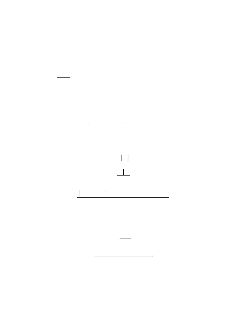
Excerpts from this work may be reproduced by instructors for distribution on a not-for-profit basis for testing or instructional purposes only to
students enrolled in courses for which the textbook has been adopted. Any other reproduction or translation of this work beyond that permitted
by Sections 107 or 108 of the 1976 United States Copyright Act without the permission of the copyright owner is unlawful.
The Hall Effect
18.41 Some hypothetical metal is known to have an electrical resistivity of 4
× 10
-8
(
Ω-m). Through a
specimen of this metal that is 25 mm thick is passed a current of 30 A; when a magnetic field of 0.75 tesla is
simultaneously imposed in a direction perpendicular to that of the current, a Hall voltage of -1.26
× 10
-7
V is
measured. Compute (a) the electron mobility for this metal, and (b) the number of free electrons per cubic meter.
Solution
(a) This portion of the problem calls for us to determine the electron mobility for some hypothetical metal
using the Hall effect. This metal has an electrical resistivity of 4
× 10
-8
(
Ω-m), while the specimen thickness is 25
mm, I
x
= 30 A and B
z
= 0.75 tesla; under these circumstances a Hall voltage of –1.26
× 10
-7
V is measured. It is
first necessary to convert resistivity to conductivity (Equation 18.4). Thus
σ =
1
ρ
=
1
4
× 10
−8
(
Ω − m)
= 2.5
× 10
7
(
Ω - m)
-1
The electron mobility may be determined using Equation 18.20b; and upon incorporation of Equation 18.18, we
have
µ
e
= R
H
σ
=
V
H
d
σ
I
x
B
z
=
−1.26 × 10
−7
V
(
)
(
25
× 10
−3
m
)
2.5
× 10
7
(
Ω − m)
−1
[
]
(30 A)(0.75 tesla)
= 0.0035 m
2
/V - s
(b) Now we are to calculate the number of free electrons per cubic meter. From Equation 18.8 we have
n =
σ
| e |
µ
e
=
2.5
× 10
7
(
Ω - m)
−1
(
1.602
× 10
−19
C
)(
0.0035 m
2
/V - s
)
= 4.46
× 10
28
m
-3
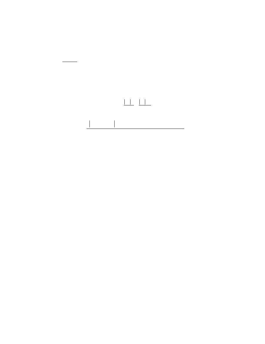
Excerpts from this work may be reproduced by instructors for distribution on a not-for-profit basis for testing or instructional purposes only to
students enrolled in courses for which the textbook has been adopted. Any other reproduction or translation of this work beyond that permitted
by Sections 107 or 108 of the 1976 United States Copyright Act without the permission of the copyright owner is unlawful.
18.42 Some metal alloy is known to have electrical conductivity and electron mobility values of 1.5
× 10
7
(
Ω-m)
-1
and 0.0020 m
2
/V-s, respectively. Through a specimen of this alloy that is 35 mm thick is passed a current of
45 A. What magnetic field would need to be imposed to yield a Hall voltage of -1.0
× 10
-7
V?
Solution
In this problem we are asked to determine the magnetic field required to produce a Hall voltage of -1.0
×
10
-7
V, given that
σ = 1.5 × 10
7
(
Ω-m)
-1
,
µ
e
= 0.0020 m
2
/V-s, I
x
= 45 A, and d = 35 mm. Combining Equations
18.18 and 18.20b, and after solving for B
z
, we get
B
z
=
V
H
d
I
x
R
H
=
V
H
σd
I
x
µ
e
=
−1.0 × 10
−7
V
(
)
1.5
× 10
7
(
Ω − m)
−1
[
]
(
35
× 10
−3
m
)
(45 A)
(
0.0020 m
2
/ V - s
)
= 0.58 tesla

Excerpts from this work may be reproduced by instructors for distribution on a not-for-profit basis for testing or instructional purposes only to
students enrolled in courses for which the textbook has been adopted. Any other reproduction or translation of this work beyond that permitted
by Sections 107 or 108 of the 1976 United States Copyright Act without the permission of the copyright owner is unlawful.
Semiconducting Devices
18.43 Briefly describe electron and hole motions in a p–n junction for forward and reverse biases; then
explain how these lead to rectification.
The explanations called for are found in Section 18.15.

Excerpts from this work may be reproduced by instructors for distribution on a not-for-profit basis for testing or instructional purposes only to
students enrolled in courses for which the textbook has been adopted. Any other reproduction or translation of this work beyond that permitted
by Sections 107 or 108 of the 1976 United States Copyright Act without the permission of the copyright owner is unlawful.
18.44 How is the energy in the reaction described by Equation 18.21 dissipated?
Solution
The energy generated by the electron-hole annihilation reaction, Equation 18.21, is dissipated as heat.

Excerpts from this work may be reproduced by instructors for distribution on a not-for-profit basis for testing or instructional purposes only to
students enrolled in courses for which the textbook has been adopted. Any other reproduction or translation of this work beyond that permitted
by Sections 107 or 108 of the 1976 United States Copyright Act without the permission of the copyright owner is unlawful.
18.45 What are the two functions that a transistor may perform in an electronic circuit?
Solution
In an electronic circuit, a transistor may be used to (1) amplify an electrical signal, and (2) act as a
switching device in computers.

Excerpts from this work may be reproduced by instructors for distribution on a not-for-profit basis for testing or instructional purposes only to
students enrolled in courses for which the textbook has been adopted. Any other reproduction or translation of this work beyond that permitted
by Sections 107 or 108 of the 1976 United States Copyright Act without the permission of the copyright owner is unlawful.
18.46 Cite the differences in operation and application for junction transistors and MOSFETs.
The differences in operation and application for junction transistors and MOSFETs are described in
Section 18.15.

Excerpts from this work may be reproduced by instructors for distribution on a not-for-profit basis for testing or instructional purposes only to
students enrolled in courses for which the textbook has been adopted. Any other reproduction or translation of this work beyond that permitted
by Sections 107 or 108 of the 1976 United States Copyright Act without the permission of the copyright owner is unlawful.
Conduction in Ionic Materials
18.47 We noted in Section 12.5 (Figure 12.22) that in FeO (wüstite), the iron ions can exist in both Fe
2+
and Fe
3+
states. The number of each of these ion types depends on temperature and the ambient oxygen pressure.
Furthermore, we also noted that in order to retain electroneutrality, one Fe
2+
vacancy will be created for every two
Fe
3+
ions that are formed; consequently, in order to reflect the existence of these vacancies the formula for wüstite
is often represented as Fe
(1 – x)
O where x is some small fraction less than unity.
In this nonstoichiometric Fe
(1 – x)
O material, conduction is electronic, and, in fact, it behaves as a p-type
semiconductor. That is, the Fe
3+
ions act as electron acceptors, and it is relatively easy to excite an electron from
the valence band into an Fe
3+
acceptor state, with the formation of a hole. Determine the electrical conductivity of a
specimen of wüstite that has a hole mobility of 1.0 × 10
–5
m
2
/V-s and for which the value of x is 0.060. Assume that
the acceptor states are saturated (i.e., one hole exists for every Fe
3+
ion). Wüstite has the sodium chloride crystal
structure with a unit cell edge length of 0.437 nm.
Solution
We are asked in this problem to determine the electrical conductivity for the nonstoichiometric Fe
(1 - x)
O,
given x = 0.060 and that the hole mobility is 1.0
× 10
-5
m
2
/V-s. It is first necessary to compute the number of
vacancies per cubic meter for this material. For this determination let us use as our basis 10 unit cells. For the
sodium chloride crystal structure there are four cations and four anions per unit cell. Thus, in ten unit cells of FeO
there will normally be forty O
2-
and forty Fe
2+
ions. However, when x = 0.06, (0.06)(40) = 2.4 of the Fe
2+
sites
will be vacant. (Furthermore, there will be 4.8 Fe
3+
ions in these ten unit cells inasmuch as two Fe
3+
ions are
created for every vacancy). Therefore, each unit cell will, on the average contain 0.24 vacancies. Now, the number
of vacancies per cubic meter is just the number of vacancies per unit cell divided by the unit cell volume; this
volume is just the unit cell edge length (0.437 nm) cubed. Thus
# vacancies
m
3
=
0.24 vacancies / unit cell
(
0.437
× 10
−9
m
)
3
= 2.88
× 10
27
vacancies/m
3
Inasmuch as it is assumed that the vacancies are saturated, the number of holes (p) is also 2.88
× 10
27
m
-3
. It is
now possible, using Equation 18.17, to compute the electrical conductivity of this material as
σ = p| e |µ
h
=
(
2.88
× 10
27
m
-3
)(
1.602
× 10
-19
C
)(
1.0
× 10
-5
m
2
/V - s
)
= 4613 (
Ω - m)
-1

Excerpts from this work may be reproduced by instructors for distribution on a not-for-profit basis for testing or instructional purposes only to
students enrolled in courses for which the textbook has been adopted. Any other reproduction or translation of this work beyond that permitted
by Sections 107 or 108 of the 1976 United States Copyright Act without the permission of the copyright owner is unlawful.
18.48 At temperatures between 775
°C (1048 K) and 1100°C (1373 K), the activation energy and
preexponential for the diffusion coefficient of Fe
2+
in FeO are 102,000 J/mol and 7.3
× 10
-8
m
2
/s, respectively.
Compute the mobility for an Fe
2+
ion at 1000
°C (1273 K).
Solution
For this problem, we are given, for FeO, the activation energy (102,000 J/mol) and preexponential (7.3
×
10
-8
m
2
/s) for the diffusion coefficient of Fe
2+
and are asked to compute the mobility for a Fe
2+
ion at 1273 K. The
mobility,
µ
Fe
2+
, may be computed using Equation 18.23; however, this expression also includes the diffusion
coefficient D
Fe
2+
, which is determined using Equation 5.8 as
D
Fe
2+
= D
0
exp
−
Q
d
RT
=
(
7.3
× 10
-8
m
2
/s
)
exp
−
102, 000 J / mol
(8.31 J/mol - K)(1273 K)
= 4.74
× 10
-12
m
2
/s
Now solving for
µ
Fe
2+
yields
µ
Fe
2
+
=
n
Fe
2
+
e D
Fe
2
+
kT
=
(2 )
(
1.602
× 10
−19
C / atom
)(
4.74
× 10
−12
m
2
/s
)
(
1.38
× 10
−23
J/atom - K
)
(1273 K)
= 8.64
× 10
-11
m
2
/V - s
(Note: the value of n
Fe2+
is two, inasmuch as two electrons are involved in the ionization of Fe to Fe
2+
.)
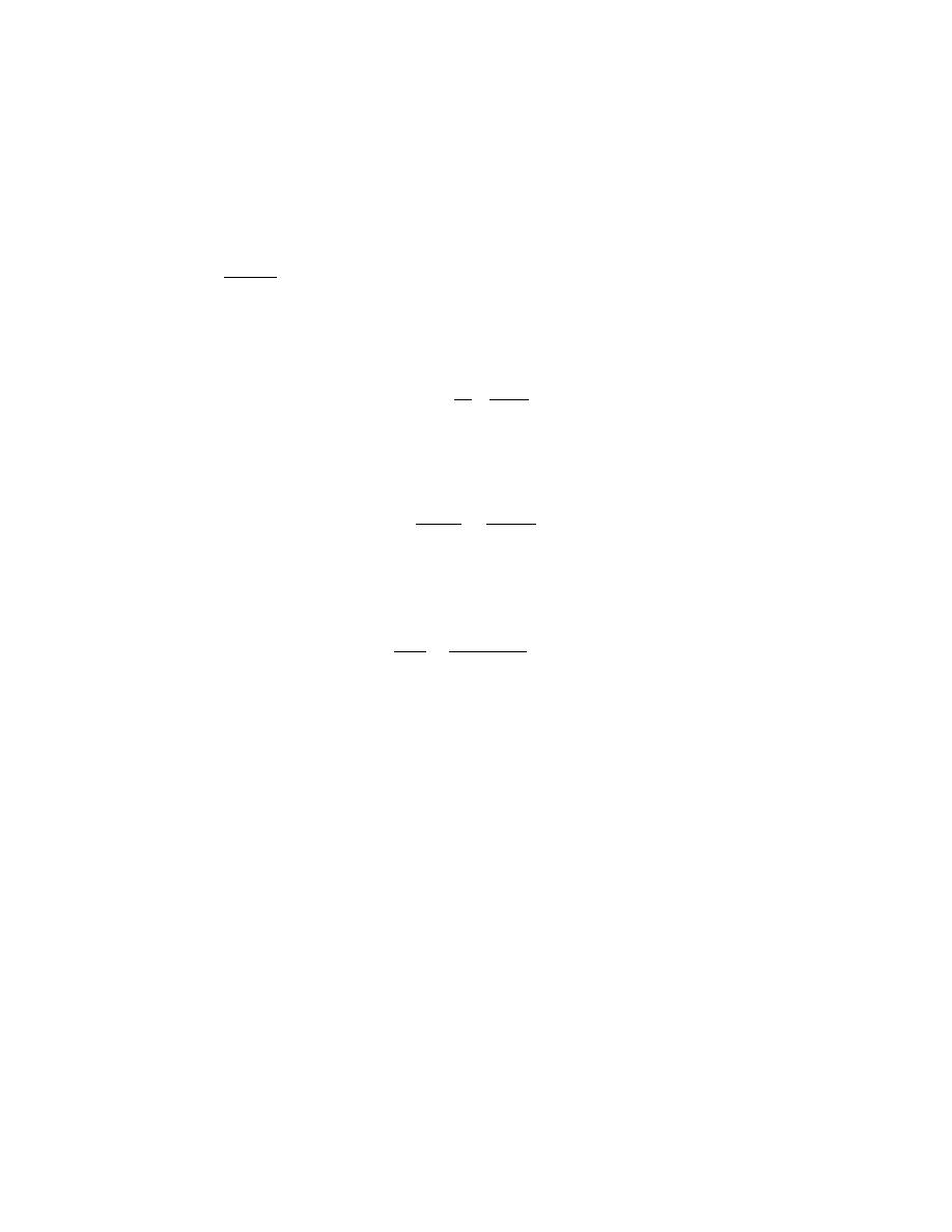
Excerpts from this work may be reproduced by instructors for distribution on a not-for-profit basis for testing or instructional purposes only to
students enrolled in courses for which the textbook has been adopted. Any other reproduction or translation of this work beyond that permitted
by Sections 107 or 108 of the 1976 United States Copyright Act without the permission of the copyright owner is unlawful.
Capacitance
18.49 A parallel-plate capacitor using a dielectric material having an
ε
r
of 2.5 has a plate spacing of 1
mm (0.04 in.). If another material having a dielectric constant of 4.0 is used and the capacitance is to be
unchanged, what must be the new spacing between the plates?
Solution
We want to compute the plate spacing of a parallel-plate capacitor as the dielectric constant is increased
form 2.5 to 4.0, while maintaining the capacitance constant. Combining Equations 18.26 and 18.27 yields
C
=
εA
l
=
ε
r
ε
0
A
l
Now, let us use the subscripts 1 and 2 to denote the initial and final states, respectively. Since C
1
= C
2
, then
ε
r1
ε
0
A
l
1
=
ε
r2
ε
0
A
l
2
And, solving for l
2
l
2
=
ε
r2
l
1
ε
r1
=
(4.0)(1 mm)
2.5
= 1.6 mm

Excerpts from this work may be reproduced by instructors for distribution on a not-for-profit basis for testing or instructional purposes only to
students enrolled in courses for which the textbook has been adopted. Any other reproduction or translation of this work beyond that permitted
by Sections 107 or 108 of the 1976 United States Copyright Act without the permission of the copyright owner is unlawful.
18.50 A parallel-plate capacitor with dimensions of 100 mm by 25 mm and a plate separation of 3 mm
must have a minimum capacitance of 38 pF (3.8
× 10
-11
F) when an ac potential of 500 V is applied at a frequency
of 1 MHz. Which of those materials listed in Table 18.5 are possible candidates? Why?
Solution
This problem asks for us to ascertain which of the materials listed in Table 18.5 are candidates for a
parallel-plate capacitor that has dimensions of 100 mm by 25 mm, a plate separation of 3 mm so as to have a
minimum capacitance of 3.8
× 10
-11
F, when an ac potential of 500 V is applied at 1 MHz. Upon combining
Equations 18.26 and 18.27 and solving for the dielectric constant
ε
r
we get
ε
r
=
ε
ε
0
=
l C
ε
0
A
=
(
3
× 10
−3
m
)(
3.8
× 10
−11
F
)
(
8.85
× 10
−12
F / m
)(
100
× 10
−3
m
)(
25
× 10
−3
m
)
= 5.15
Thus, the minimum value of
ε
r
to achieve the desired capacitance is 5.15 at 1 MHz. Of those materials listed in the
table, titanate ceramics, mica, steatite, soda-lime glass, and porcelain are candidates.

Excerpts from this work may be reproduced by instructors for distribution on a not-for-profit basis for testing or instructional purposes only to
students enrolled in courses for which the textbook has been adopted. Any other reproduction or translation of this work beyond that permitted
by Sections 107 or 108 of the 1976 United States Copyright Act without the permission of the copyright owner is unlawful.
18.51 Consider a parallel-plate capacitor having an area of 2500 mm
2
and a plate separation of 2 mm,
and with a material of dielectric constant 4.0 positioned between the plates. (a) What is the capacitance of this
capacitor? (b) Compute the electric field that must be applied for 8.0
× 10
-9
C to be stored on each plate.
Solution
In this problem we are given, for a parallel-plate capacitor, its area (2500 mm
2
), the plate separation (2
mm), and that a material having an
ε
r
of 4.0 is positioned between the plates.
(a) We are first asked to compute the capacitance. Combining Equations 18.26 and 18.27, and solving for
C yields
C =
εA
l
=
ε
r
ε
0
A
l
=
(4.0)
(
8.85
× 10
−12
F / m
)(
2500 mm
2
)(
1 m
2
/10
6
mm
2
)
2
× 10
−3
m
= 4.43
× 10
-11
F = 44.3 pF
(b) Now we are asked to compute the electric field that must be applied in order that 8
× 10
-9
C be stored
on each plate. First we need to solve for V in Equation 18.24 as
V =
Q
C
=
8
× 10
−9
C
4.43
× 10
−11
F
= 181 V
The electric field E may now be determined using Equation 18.6; thus
E =
V
l
=
181 V
2
× 10
−3
m
= 9.1
× 10
4
V/m

Excerpts from this work may be reproduced by instructors for distribution on a not-for-profit basis for testing or instructional purposes only to
students enrolled in courses for which the textbook has been adopted. Any other reproduction or translation of this work beyond that permitted
by Sections 107 or 108 of the 1976 United States Copyright Act without the permission of the copyright owner is unlawful.
18.52 In your own words, explain the mechanism by which charge storing capacity is increased by the
insertion of a dielectric material within the plates of a capacitor.
This explanation is found in Section 18.19.
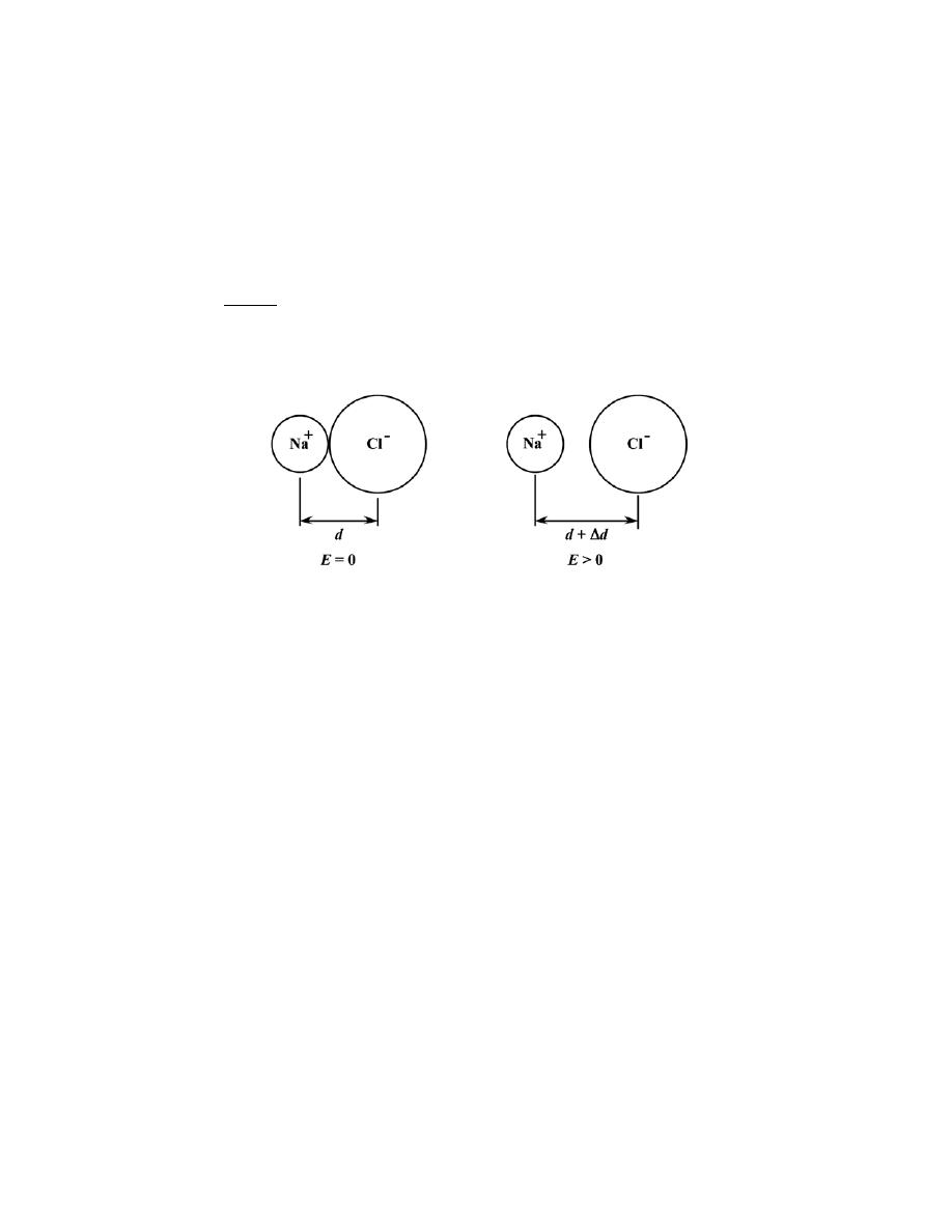
Excerpts from this work may be reproduced by instructors for distribution on a not-for-profit basis for testing or instructional purposes only to
students enrolled in courses for which the textbook has been adopted. Any other reproduction or translation of this work beyond that permitted
by Sections 107 or 108 of the 1976 United States Copyright Act without the permission of the copyright owner is unlawful.
Field Vectors and Polarization
Types of Polarization
18.53 For NaCl, the ionic radii for Na
+
and Cl
-
ions are 0.102 and 0.181 nm, respectively. If an
externally applied electric field produces a 5% expansion of the lattice, compute the dipole moment for each Na
+
–
Cl
-
pair. Assume that this material is completely unpolarized in the absence of an electric field.
Solution
Shown below are the relative positions of Na
+
and Cl
-
ions, without and with an electric field present.
Now,
d = r
Na
+
+ r
Cl-
= 0.102 nm + 0.181 nm = 0.283 nm
and
∆d = 0.05 d = (0.05)(0.283 nm) = 0.0142 nm = 1.42 × 10
-11
m
From Equation 18.28, the dipole moment, p, is just
p = q
∆d
=
(
1.602
× 10
-19
C
)(
1.42
× 10
-11
m
)
= 2.26
× 10
-30
C-m

Excerpts from this work may be reproduced by instructors for distribution on a not-for-profit basis for testing or instructional purposes only to
students enrolled in courses for which the textbook has been adopted. Any other reproduction or translation of this work beyond that permitted
by Sections 107 or 108 of the 1976 United States Copyright Act without the permission of the copyright owner is unlawful.
18.54 The polarization P of a dielectric material positioned within a parallel-plate capacitor is to be 1.0
×
10
-6
C/m
2
.
(a) What must be the dielectric constant if an electric field of 5
× 10
4
V/m is applied?
(b) What will be the dielectric displacement D?
Solution
(a) In order to solve for the dielectric constant in this problem, we must employ Equation 18.32, in which
the polarization and the electric field are given. Solving for
ε
r
from this expression gives
ε
r
=
P
ε
0
E
+ 1
=
1.0
× 10
−6
C / m
2
(
8.85
× 10
−12
F / m
)(
5
× 10
4
V / m
)
+ 1
= 3.26
(b) The dielectric displacement may be determined using Equation 18.31, as
D =
ε
0
E + P
=
(
8.85
× 10
-12
F/m
)(
5
× 10
4
V/m
)
+ 1.0
× 10
-6
C/m
2
= 1.44
× 10
-6
C/m
2

Excerpts from this work may be reproduced by instructors for distribution on a not-for-profit basis for testing or instructional purposes only to
students enrolled in courses for which the textbook has been adopted. Any other reproduction or translation of this work beyond that permitted
by Sections 107 or 108 of the 1976 United States Copyright Act without the permission of the copyright owner is unlawful.
18.55 A charge of 3.5
× 10
-11
C is to be stored on each plate of a parallel-plate capacitor having an area of
160 mm
2
(0.25 in.
2
) and a plate separation of 3.5 mm (0.14 in.).
(a) What voltage is required if a material having a dielectric constant of 5.0 is positioned within the
plates?
(b) What voltage would be required if a vacuum were used?
(c) What are the capacitances for parts (a) and (b)?
(d) Compute the dielectric displacement for part (a).
(e) Compute the polarization for part (a).
Solution
(a) We want to solve for the voltage when Q = 3.5
× 10
-11
C, A = 160 mm
2
, l = 3.5 mm, and
ε
r
= 5.0.
Combining Equations 18.24, 18.26, and 18.27 yields
C =
Q
V
=
ε
A
l
= ε
r
ε
0
A
l
Or
Q
V
=
ε
r
ε
0
A
l
And, solving for V, and incorporating values provided in the problem statement, leads to
V =
Q l
ε
r
ε
0
A
=
(
3.5
× 10
−11
C
)(
3.5
× 10
−3
m
)
(5.0)
(
8.85
× 10
−12
F / m
)(
160 mm
2
)(
1 m
2
/10
6
mm
2
)
= 17.3 V
(b) For this same capacitor, if a vacuum is used
V =
Q l
ε
0
A
=
(
3.5
× 10
−11
C
)(
3.5
× 10
−3
m
)
(
8.85
× 10
−12
F / m
)(
160
× 10
−6
m
2
)

Excerpts from this work may be reproduced by instructors for distribution on a not-for-profit basis for testing or instructional purposes only to
students enrolled in courses for which the textbook has been adopted. Any other reproduction or translation of this work beyond that permitted
by Sections 107 or 108 of the 1976 United States Copyright Act without the permission of the copyright owner is unlawful.
= 86.5 V
(c) The capacitance for part (a) is just
C =
Q
V
=
3.5
× 10
−11
C
17.3 V
= 2.0
× 10
-12
F
While for part (b)
C =
Q
V
=
3.5
× 10
−11
C
86.5 V
= 4.0
× 10
-13
F
(d) The dielectric displacement may be computed by combining Equations 18.31, 18.32 and 18.6, as
D =
ε
0
E + P =
ε
0
E +
ε
0
(
ε
r
− 1)E = ε
0
ε
rE =
ε
0
ε
r
V
l
And incorporating values for
ε
r
and l provided in the problem statement, as well as the value of V computed in part
(a)
D =
(
8.85
× 10
−12
F / m
)
(5.0)(17.3 V)
3.5
× 10
−3
m
= 2.2
× 10
-7
C/m
2
(e) The polarization is determined using Equations 18.32 and 18.6 as
P =
ε
0
(
ε
r
− 1)E = ε
0
(
ε
r
− 1)
V
l
=
(
8.85
× 10
−12
F / m
)
(5.0
− 1)(17.3 V)
3.5
× 10
−3
m
= 1.75
× 10
-7
C/m
2

Excerpts from this work may be reproduced by instructors for distribution on a not-for-profit basis for testing or instructional purposes only to
students enrolled in courses for which the textbook has been adopted. Any other reproduction or translation of this work beyond that permitted
by Sections 107 or 108 of the 1976 United States Copyright Act without the permission of the copyright owner is unlawful.
18.56 (a) For each of the three types of polarization, briefly describe the mechanism by which dipoles are
induced and/or oriented by the action of an applied electric field. (b) For solid lead titanate (PbTiO
3
), gaseous
neon, diamond, solid KCl, and liquid NH
3
what kind(s) of polarization is (are) possible? Why?
Solution
(a) For electronic polarization, the electric field causes a net displacement of the center of the negatively
charged electron cloud relative to the positive nucleus. With ionic polarization, the cations and anions are displaced
in opposite directions as a result of the application of an electric field. Orientation polarization is found in
substances that possess permanent dipole moments; these dipole moments become aligned in the direction of the
electric field.
(b) Electronic, ionic, and orientation polarizations would be observed in lead titanate. The lead, titanium,
and oxygen would undoubtedly be largely ionic in character. Furthermore, orientation polarization is also possible
inasmuch as permanent dipole moments may be induced in the same manner as for BaTiO
3
as shown in Figure
18.35.
Only electronic polarization is to be found in gaseous neon; being an inert gas, its atoms will not be
ionized nor possess permanent dipole moments.
Only electronic polarization is to be found in solid diamond; this material does not have molecules with
permanent dipole moments, nor is it an ionic material.
Both electronic and ionic polarizations will be found in solid KCl, since it is strongly ionic. In all
probability, no permanent dipole moments will be found in this material.
Both electronic and orientation polarizations are found in liquid NH
3
. The NH
3
molecules have permanent
dipole moments that are easily oriented in the liquid state.

Excerpts from this work may be reproduced by instructors for distribution on a not-for-profit basis for testing or instructional purposes only to
students enrolled in courses for which the textbook has been adopted. Any other reproduction or translation of this work beyond that permitted
by Sections 107 or 108 of the 1976 United States Copyright Act without the permission of the copyright owner is unlawful.
18.57 (a) Compute the magnitude of the dipole moment associated with each unit cell of BaTiO
3
, as
illustrated in Figure 18.35.
(b) Compute the maximum polarization that is possible for this material.
Solution
(a) This portion of the problem asks that we compute the magnitude of the dipole moment associated with
each unit cell of BaTiO
3
, which is illustrated in Figure 18.35. The dipole moment p is defined by Equation 18.28 as
p = qd in which q is the magnitude of each dipole charge, and d is the distance of separation between the charges.
Each Ti
4+
ion has four units of charge associated with it, and thus q = (4)(1.602
× 10
-19
C) = 6.41
× 10
-19
C.
Furthermore, d is the distance the Ti
4+
ion has been displaced from the center of the unit cell, which is just 0.006
nm + 0.006 nm = 0.012 nm [Figure 18.35(b)]. Hence
p = qd =
(
6.41
× 10
-19
C
)(
0.012
× 10
-9
m
)
= 7.69
× 10
-30
C-m
(b) Now it becomes necessary to compute the maximum polarization that is possible for this material. The
maximum polarization will exist when the dipole moments of all unit cells are aligned in the same direction.
Furthermore, it is computed by dividing the above value of p by the volume of each unit cell, which is equal to the
product of three unit cell edge lengths, as shown in Figure 18.35. Thus
P =
p
V
C
=
7.69
× 10
−30
C
− m
(
0.403
× 10
−9
m
)(
0.398
× 10
−9
m
)(
0.398
× 10
−9
m
)
= 0.121 C/m
2

Excerpts from this work may be reproduced by instructors for distribution on a not-for-profit basis for testing or instructional purposes only to
students enrolled in courses for which the textbook has been adopted. Any other reproduction or translation of this work beyond that permitted
by Sections 107 or 108 of the 1976 United States Copyright Act without the permission of the copyright owner is unlawful.
Frequency Dependence of the Dielectric Constant
18.58 The dielectric constant for a soda–lime glass measured at very high frequencies (on the order of
10
15
Hz) is approximately 2.3. What fraction of the dielectric constant at relatively low frequencies (1 MHz) is
attributed to ionic polarization? Neglect any orientation polarization contributions.
Solution
For this soda-lime glass, in order to compute the fraction of the dielectric constant at low frequencies that is
attributed to ionic polarization, we must determine the
ε
r
within this low-frequency regime; such is tabulated in
Table 18.5, and at 1 MHz its value is 6.9. Thus, this fraction is just
fraction =
ε
r
(low)
− ε
r
(high)
ε
r
(low)
=
6.9
− 2.3
6.9
= 0.67

Excerpts from this work may be reproduced by instructors for distribution on a not-for-profit basis for testing or instructional purposes only to
students enrolled in courses for which the textbook has been adopted. Any other reproduction or translation of this work beyond that permitted
by Sections 107 or 108 of the 1976 United States Copyright Act without the permission of the copyright owner is unlawful.
Ferroelectricity
18.59 Briefly explain why the ferroelectric behavior of BaTiO
3
ceases above its ferroelectric Curie
temperature.
Solution
The ferroelectric behavior of BaTiO
3
ceases above its ferroelectric Curie temperature because the unit cell
transforms from tetragonal geometry to cubic; thus, the Ti
4+
is situated at the center of the cubic unit cell, there is
no charge separation, and no net dipole moment.

Excerpts from this work may be reproduced by instructors for distribution on a not-for-profit basis for testing or instructional purposes only to
students enrolled in courses for which the textbook has been adopted. Any other reproduction or translation of this work beyond that permitted
by Sections 107 or 108 of the 1976 United States Copyright Act without the permission of the copyright owner is unlawful.
DESIGN PROBLEMS
Electrical Resistivity of Metals
18.D1 A 95 wt% Pt-5 wt% Ni alloy is known to have an electrical resistivity of 2.35
× 10
-7
Ω-m at room
temperature (25
°C). Calculate the composition of a platinum-nickel alloy that gives a room-temperature resistivity
of 1.75
× 10
-7
Ω-m. The room-temperature resistivity of pure platinum may be determined from the data in Table
18.1; assume that platinum and nickel form a solid solution.
Solution
This problem asks that we calculate the composition of a platinum-nickel alloy that has a room temperature
resistivity of 1.75
× 10
-7
Ω-m. The first thing to do is, using the 95 Pt-5 Ni resistivity data, determine the impurity
contribution, and, from this result, calculate the constant A in Equation 18.11. Thus,
ρ
total
= 2.35
× 10
-7
(
Ω - m) = ρ
i
+
ρ
t
From Table 18.1, for pure platinum, and using Equation 18.4
ρ
t
=
1
σ
=
1
0.94
× 10
7
(
Ω − m)
−1
= 1.064
× 10
-7
(
Ω - m)
Thus, for the 95 Pt-5 Ni alloy
ρ
i
=
ρ
total
− ρ
t
= 2.35
× 10
-7
− 1.064 × 10
-7
= 1.286
× 10
-7
(
Ω-m)
In the problem statement, the impurity (i.e., nickel) concentration is expressed in weight percent. However,
Equation 18.11 calls for concentration in atom fraction (i.e., atom percent divided by 100). Consequently,
conversion from weight percent to atom fraction is necessary. (Note: we now choose to denote the atom fraction of
nickel as
c
Ni
' , and the weight percents of Ni and Pt by C
Ni
and C
Pt
, respectively.) Using these notations, this
conversion may be accomplished by using a modified form of Equation 4.6a as
c
Ni
' =
C
Ni
'
100
=
C
Ni
A
Pt
C
Ni
A
Pt
+ C
Pt
A
Ni

Excerpts from this work may be reproduced by instructors for distribution on a not-for-profit basis for testing or instructional purposes only to
students enrolled in courses for which the textbook has been adopted. Any other reproduction or translation of this work beyond that permitted
by Sections 107 or 108 of the 1976 United States Copyright Act without the permission of the copyright owner is unlawful.
Here A
Ni
and A
Pt
denote the atomic weights of nickel and platinum (which values are 58.69 and 195.08 g/mol,
respectively). Thus
c
Ni
' =
(5 wt%)(195.08 g / mol)
(5 wt%)(195.08 g / mol)
+ (95 wt%)(58.69 g /mol)
= 0.15
Now, solving for A in Equation 18.11
A =
ρ
i
c
Ni
' 1
− c
Ni
'
=
1.286
× 10
−7
(
Ω − m)
(0.15)(1
− 0.15)
= 1.01
× 10
-6
(
Ω - m)
Now it is possible to compute the
c
Ni
' to give a room temperature resistivity of 1.75
× 10
-7
Ω-m. Again, we must
determine
ρ
i
as
ρ
i
=
ρ
total
− ρ
t
= 1.75
× 10
-7
− 1.286 × 10
-7
= 4.64
× 10
-8
(
Ω - m)
If Equation 18.11 is expanded, then
ρ
i
= A c
Ni
'
− A c
Ni
'
2
Or, rearranging this equation, we have
A c
Ni
'
2
− A c
Ni
'
+ ρ
i
= 0
Now, solving for
c
Ni
' (using the quadratic equation solution)
Excerpts from this work may be reproduced by instructors for distribution on a not-for-profit basis for testing or instructional purposes only to
students enrolled in courses for which the textbook has been adopted. Any other reproduction or translation of this work beyond that permitted
by Sections 107 or 108 of the 1976 United States Copyright Act without the permission of the copyright owner is unlawful.
c
Ni
' =
A
± A
2
− 4 Aρ
i
2 A
Again, from the above
A = 1.01
× 10
-6
(
Ω-m)
ρ
i
= 4.64
× 10
-8
(
Ω-m)
which leads to
c
Ni
' =
1.01
× 10
−6
±
(
1.01
× 10
−6
)
2
− (4)
(
1.01
× 10
−6
)(
4.64
× 10
−8
)
(2)
(
1.01
× 10
−6
)
And, taking the negative root,
c
Ni
' = 0.0483
Or, in terms of atom percent,
C
Ni
Õ
= 100c
Ni
Õ
= (100)(0.0483) = 4.83 at%
While the concentration of platinum is
C
Pt
Õ
= 100 − C
Ni
Õ
= 100.00 − 4.83 = 95.17 at%
Now, converting this composition to weight percent Ni, requires that we use Equation 4.7a as
C
Ni
=
C
Ni
' A
Ni
C
Ni
' A
Ni
+ C
Pt
' A
PT
× 100
=
(4.83 at%)(58.69 g / mol)
(4.83 at%)(58.69 g / mol)
+ (95.17 at%)(195.08 g /mol)
× 100
= 1.50 wt%

Excerpts from this work may be reproduced by instructors for distribution on a not-for-profit basis for testing or instructional purposes only to
students enrolled in courses for which the textbook has been adopted. Any other reproduction or translation of this work beyond that permitted
by Sections 107 or 108 of the 1976 United States Copyright Act without the permission of the copyright owner is unlawful.
18.D2 Using information contained in Figures 18.8 and 18.38, determine the electrical conductivity of an
80 wt% Cu-20 wt% Zn alloy at -150
°C (-240°F).
Solution
This problem asks that we determine the electrical conductivity of an 80 wt% Cu-20 wt% Zn alloy at
–150
°C using information contained in Figures 18.8 and 18.38. In order to solve this problem it is necessary to
employ Equation 18.9 which is of the form
ρ
total
=
ρ
t
+
ρ
i
since it is assumed that the alloy is undeformed. Let us first determine the value of
ρ
i
at room temperature (25
°C)
which value will be independent of temperature. From Figure 18.8, at 25
°C and for pure Cu, ρ
t
(25) = 1.75
× 10
-8
Ω-m. Now, since it is assumed that the curve in Figure 18.38 was generated also at room temperature, we may take
ρ as ρ
total
(25) at 80 wt% Cu-20 wt% Zn which has a value of 5.3
× 10
-8
Ω-m. Thus
ρ
i
=
ρ
total
(25)
− ρ
t
(25)
= 5.3
× 10
-8
Ω - m − 1.75 × 10
-8
Ω - m = 3.55 × 10
-8
Ω - m
Finally, we may determine the resistivity at –150
°C, ρ
total
(–150), by taking the resistivity of pure Cu at –150
°C
from Figure 18.8, which gives us
ρ
t
(–150) = 0.55
× 10
-8
Ω-m. Therefore
ρ
total
(
−150) = ρ
i
+
ρ
t
(
−150)
= 3.55
× 10
-8
Ω - m + 0.55 × 10
-8
Ω - m = 4.10 × 10
-8
Ω - m
And, using Equation 18.4 the conductivity is calculated as
σ =
1
ρ
=
1
4.10
× 10
−8
Ω − m
= 2.44
× 10
7
(
Ω - m)
-1

Excerpts from this work may be reproduced by instructors for distribution on a not-for-profit basis for testing or instructional purposes only to
students enrolled in courses for which the textbook has been adopted. Any other reproduction or translation of this work beyond that permitted
by Sections 107 or 108 of the 1976 United States Copyright Act without the permission of the copyright owner is unlawful.
18.D3 Is it possible to alloy copper with nickel to achieve a minimum tensile strength of 375 MPa (54,400
psi) and yet maintain an electrical conductivity of 2.5
× 10
6
(
Ω-m)
-1
? If not, why? If so, what concentration of
nickel is required? You may want to consult Figure 7.16a.
Solution
To solve this problem, we want to consult Figures 7.16a and 18.9 in order to determine the Ni
concentration ranges over which the tensile strength is greater than 375 MPa (54,500 psi) and the conductivity
exceeds 2.5
× 10
6
(
Ω-m)
-1
.
From Figure 7.16a, a Ni concentration greater than about 30 wt% is necessary for a tensile strength in
excess of 375 MPa. In Figure 18.9 is plotted the resistivity versus the Ni content. Since conductivity is the
reciprocal of resistivity, the resistivity must be less than 40
× 10
-8
Ω-m--i.e.,
1
2.5
× 10
6
(
Ω − m)
−1
. According to
the figure, this will be the case for Ni concentrations less than 32.5 wt%.
Hence, it is possible to prepare an alloy meeting the criteria. The concentration of Ni would have to lie
between about 30 and 32.5 wt%.

Excerpts from this work may be reproduced by instructors for distribution on a not-for-profit basis for testing or instructional purposes only to
students enrolled in courses for which the textbook has been adopted. Any other reproduction or translation of this work beyond that permitted
by Sections 107 or 108 of the 1976 United States Copyright Act without the permission of the copyright owner is unlawful.
Extrinsic Semiconduction
Factors That Affect Carrier Mobility
18.D4 Specify an acceptor impurity type and concentration (in weight percent) that will produce a p-type
silicon material having a room temperature electrical conductivity of 50 (
Ω-m)
-1
.
Solution
First of all, those elements which, when added to silicon render it p-type, lie one group to the left of silicon
in the periodic table; these include the group IIIA elements (Figure 2.6)--i.e., boron, aluminum, gallium, and
indium.
Since this material is extrinsic and p-type, p >> n, and the electrical conductivity is a function of the hole
concentration according to Equation 18.17. Also, the number of holes is about equal to the number of acceptor
impurities, N
a
. That is
p ~ N
a
From Equation 18.17, the conductivity is a function of both the hole concentration (p) and the hole mobility (
µ
h
).
Furthermore, the room-temperature hole mobility is dependent on impurity concentration (Figure 18.18). One way
to solve this problem is to use an iterative approach—i.e., assume some acceptor impurity concentration (which will
also equal the value of p), then determine a "calculated" hole mobility from Equation 18.17—i.e.,
µ
h
=
σ
p | e |
and, finally, compare this mobility with the "measured" value from Figure 18.18, taken at the assumed p (i.e., N
a
)
value.
Let us begin by assuming that N
a
= 10
22
m
-3
. Thus, the "calculated" mobility value is
µ
h
=
σ
p | e |
=
50 (
Ω − m)
−1
(
10
22
m
−3
)(
1.602
× 10
−19
C
)
= 0.0312 m
2
/ V
− s
From Figure 18.18, at an impurity concentration of 10
22
m
-3
the "measured" hole mobility is 0.0362 m
2
/V-s, which
is slightly higher than the "calculated" value.
For our next choice, let us assume a lower impurity concentration, say 5
× 10
21
m
-3
. At this lower
concentration there will be an increase of both "calculated" and "measured" electron mobilities. The "calculated"
value is just
Excerpts from this work may be reproduced by instructors for distribution on a not-for-profit basis for testing or instructional purposes only to
students enrolled in courses for which the textbook has been adopted. Any other reproduction or translation of this work beyond that permitted
by Sections 107 or 108 of the 1976 United States Copyright Act without the permission of the copyright owner is unlawful.
µ
h
=
σ
p | e |
=
50 (
Ω − m)
−1
(
5
× 10
21
m
−3
)(
1.602
× 10
−19
C
)
= 0.0624 m
2
/ V
− s
Whereas, Figure 18.18 yields a "measured"
µ
h
of 0.0394 m
2
/V-s, which is lower than the "calculated" value.
Therefore, the correct impurity concentration will lie somewhere between 5
× 10
21
and 10
22
m
-3
probably closer to
the latter of these two values. At 8.0
× 10
22
m
-3
, both "measured" and "calculated"
µ
h
values are about equal
(0.039 m
2
/V-s).
It next becomes necessary to calculate the concentration of acceptor impurities in atom percent. This
computation first requires the determination of the number of silicon atoms per cubic meter, N
Si
, using Equation
4.2, which is as follows
N
Si
=
N
A
ρ
Si
'
A
Si
=
(
6.022
× 10
23
atoms / mol
)(
2.33 g / cm
3
)(
10
6
cm
3
/ m
3
)
28.09 g / mol
= 5.0
× 10
28
m
-3
(Note: in the above discussion, the density of silicon is represented by
ρ
Si
' in order to avoid confusion with
resistivity, which is designated by
ρ.)
The concentration of acceptor impurities in atom percent
(C
a
' ) is just the ratio of N
a
and (N
a
+ N
Si
)
multiplied by 100 as
C
a
Õ=
N
a
N
a
+ N
Si
× 100
=
8.0
× 10
22
m
−3
(
8.0
× 10
22
m
−3
)
+
(
5.0
× 10
28
m
−3
)
× 100 = 1.6 × 10
-4
at%
Now, conversion to weight percent (C
a
) is possible using Equation 4.7a as
C
a
=
C
a
' A
a
C
a
' A
a
+ C
Si
' A
Si
× 100

Excerpts from this work may be reproduced by instructors for distribution on a not-for-profit basis for testing or instructional purposes only to
students enrolled in courses for which the textbook has been adopted. Any other reproduction or translation of this work beyond that permitted
by Sections 107 or 108 of the 1976 United States Copyright Act without the permission of the copyright owner is unlawful.
where A
a
and A
Si
are the atomic weights of the acceptor and silicon, respectively. Thus, the concentration in weight
percent will depend on the particular acceptor type. For example, for boron
C
B
=
C
B
' A
B
C
B
' A
B
+ C
Si
' A
Si
× 100
=
(
1.6
× 10
−4
at%
)
(10.81 g / mol)
(
1.6
× 10
−4
at%
)
(10.81 g/mol)
+ (99.99984 at%)(28.09 g/mol)
× 100
= 6.16
× 10
-5
wt%
Similar calculations may be carried out for the other possible acceptor impurities which yield
C
Al
= 1.54
× 10
-4
wt%
C
Ga
= 3.97
× 10
-4
wt%
C
In
= 6.54
× 10
-4
wt%

Excerpts from this work may be reproduced by instructors for distribution on a not-for-profit basis for testing or instructional purposes only to
students enrolled in courses for which the textbook has been adopted. Any other reproduction or translation of this work beyond that permitted
by Sections 107 or 108 of the 1976 United States Copyright Act without the permission of the copyright owner is unlawful.
18.D5 One integrated circuit design calls for diffusing boron into very high purity silicon at an elevated
temperature. It is necessary that at a distance 0.2
µm from the surface of the silicon wafer, the room-temperature
electrical conductivity be 1.2
× 10
3
(
Ω-m)
-1
. The concentration of B at the surface of the Si is maintained at a
constant level of 1.0
× 10
25
m
-3
; furthermore, it is assumed that the concentration of B in the original Si material is
negligible, and that at room temperature the boron atoms are saturated. Specify the temperature at which this
diffusion heat treatment is to take place if the treatment time is to be one hour. The diffusion coefficient for the
diffusion of B in Si is a function of temperature as
D(m
2
/s) =
2.4
× 10
-4
exp
−
347 kJ/mol
RT
Solution
This problem asks for us to determine the temperature at which boron is to be diffused into high-purity
silicon in order to achieve a room-temperature electrical conductivity of 1.2
× 10
3
(
Ω-m)
-1
at a distance 0.2
µm
from the surface if the B concentration at the surface is maintained at 1.0
× 10
25
m
-3
. It is first necessary for us to
compute the hole concentration (since B is an acceptor in Si) at this 0.2
µm location.
From Equation 18.17, the conductivity is a function of both the hole concentration (p) and the hole
mobility (
µ
h
). Furthermore, the room-temperature hole mobility is dependent on impurity concentration (Figure
18.18). One way to solve this problem is to use an iterative approach—i.e., assume some boron concentration, N
B
(which will also equal the value of p), then determine a "calculated" hole mobility from Equation 18.17—i.e.,
µ
h
=
σ
p | e |
and then compare this mobility with the "measured" value from Figure 18.18, taken at the assumed p (i.e., N
B
).
Let us begin by assuming that N
B
= 10
23
m
-3
. Thus, the "calculated" mobility value is
µ
h
=
σ
p | e |
=
1.2
× 10
3
(
Ω − m)
−1
(
10
23
m
−3
)(
1.602
× 10
−19
C
)
= 0.075 m
2
/ V
− s
From Figure 18.18, at an impurity concentration of 10
23
m
-3
the "measured" hole mobility is 0.024 m
2
/V-s, which
is lower than the "calculated" value.
For our next choice, let us assume a higher boron concentration, say 10
24
m
-3
. At this higher
concentration there will be a decrease of both "calculated" and "measured" hole mobilities. The "calculated" value
is just
Excerpts from this work may be reproduced by instructors for distribution on a not-for-profit basis for testing or instructional purposes only to
students enrolled in courses for which the textbook has been adopted. Any other reproduction or translation of this work beyond that permitted
by Sections 107 or 108 of the 1976 United States Copyright Act without the permission of the copyright owner is unlawful.
µ
h
=
σ
p | e |
=
1.2
× 10
3
(
Ω − m)
−1
(
10
24
m
−3
)(
1.602
× 10
−19
C
)
= 0.0075 m
2
/ V
− s
Whereas, Figure 18.18 yields a "measured"
µ
h
of 0.01 m
2
/V-s, which is lower than the "calculated" value.
Therefore, the correct impurity concentration will lie somewhere between 10
23
and 10
24
m
-3
. At 6.0
× 10
23
m
-3
,
"measured" and "calculated" values are about equal (0.0125 m
2
/V-s).
With regard to diffusion, the problem is one involving the nonsteady-state diffusion of B into the Si,
wherein we have to solve for temperature. Temperature is incorporated into the diffusion coefficient expression
given in the problem. But we must first employ the solution to Fick's second law for constant surface composition
boundary conditions, Equation 5.5; in this expression C
0
is taken to be zero inasmuch as the problem stipulates that
the initial boron concentration may be neglected. Thus,
C
x
− C
0
C
s
− C
0
= 1
− erf
x
2 Dt
6.0
× 10
23
m
−3
− 0
1.0
× 10
25
m
−3
− 0
= 1
− erf
x
2 Dt
which reduces to
0.9400 = erf
x
2 Dt
In order to solve this expression for a value
x
2
Dt
of it is necessary to interpolate using data in Table 5.1. Thus
z
erf(z)
1.3
0.9340
z
0.9400
1.4
0.9523
z
− 1.3
1.4
− 1.3
=
0.9400
− 0.9340
0.9523
− 0.9340
Excerpts from this work may be reproduced by instructors for distribution on a not-for-profit basis for testing or instructional purposes only to
students enrolled in courses for which the textbook has been adopted. Any other reproduction or translation of this work beyond that permitted
by Sections 107 or 108 of the 1976 United States Copyright Act without the permission of the copyright owner is unlawful.
From which, z = 1.3328; which is to say
1.3328 =
x
2 Dt
Inasmuch as there are 3600 s/h (= t) and x = 0.2
µm (= 2 × 10
-7
m) the above equation becomes
1.3328 =
2
× 10
−7
m
2
(D)(3600 s)
which, when solving for the value of D, leads to
D =
1
3600 s
2
× 10
−7
m
(2)(1.3328)
2
= 1.56 × 10
−18
m
2
/s
Now, equating this value to the expression for D given in the problem gives
D = 1.56
× 10
-18
m
2
/s =
(
2.4
× 10
-4
)
exp
−
347, 000 J/mol
(8.31 J/mol - K)(T)
To solve for T, let us take the natural logarithms of both sides of the above equation; this leads to
ln
(
1.56
× 10
−18
)
= ln
(
2.4
× 10
−4
)
−
347, 000
8.31T
−41.002 = − 8.335 −
4.176
× 10
4
T
which yields a value for T of 1278 K (1005
°C).

Excerpts from this work may be reproduced by instructors for distribution on a not-for-profit basis for testing or instructional purposes only to
students enrolled in courses for which the textbook has been adopted. Any other reproduction or translation of this work beyond that permitted
by Sections 107 or 108 of the 1976 United States Copyright Act without the permission of the copyright owner is unlawful.
Conduction in Ionic Materials
18.D6 Problem 18.47 noted that FeO (wüstite) may behave as a semiconductor by virtue of the
transformation of Fe
2+
to Fe
3+
and the creation of Fe
2+
vacancies; the maintenance of electroneutrality requires
that for every two Fe
3+
ions, one vacancy is formed. The existence of these vacancies is reflected in the chemical
formula of this nonstoichiometric wüstite as Fe
(1 – x)
O, where x is a small number having a value less than unity.
The degree of nonstoichiometry (i.e., the value of x) may be varied by changing temperature and oxygen partial
pressure. Compute the value of x that is required to produce an Fe
(1 – x)
O material having a p-type electrical
conductivity of 2000 (
Ω-m)
-1
; assume that the hole mobility is 1.0
× 10
-5
m
2
/V-s, the crystal structure for FeO is
sodium chloride (with a unit cell edge length of 0.437 nm), and that the acceptor states are saturated.
Solution
This problem asks, for the nonstoichiometric Fe
(1 - x)
O, given the electrical conductivity [2000 (
Ω-m)
-1
]
and hole mobility (1.0
× 10
-5
m
2
/V-s) that we determine the value of x. It is first necessary to compute the number
of holes per unit volume (p) using Equation 18.17. Thus
p =
σ
| e |
µ
h
=
2000 (
Ω − m)
-1
(
1.602
× 10
−19
C
)(
1.0
× 10
−5
m
2
/ V - s
)
= 1.25
× 10
27
holes/m
3
Inasmuch as it is assumed that the acceptor states are saturated, the number of vacancies is also 1.25
× 10
27
m
-3
.
Next, it is possible to compute the number of vacancies per unit cell by taking the product of the number of
vacancies per cubic meter times the volume of a unit cell. This volume is just the unit cell edge length (0.437 nm)
cubed:
# vacancies
unit cell
=
(
1.25
× 10
27
m
−3
)(
0.437
× 10
−9
m
)
3
= 0.10
A unit cell for the sodium chloride structure contains the equivalence of four cations and four anions. Thus, if we
take as a basis for this problem 10 unit cells, there will be one vacancy, 40 O
2-
ions, and 39 iron ions (since one of
the iron sites is vacant). (It should also be noted that since two Fe
3+
ions are created for each vacancy, that of the 39
iron ions, 37 of them are Fe
2+
and 2 of them are Fe
3+
). In order to find the value of (1 – x) in the chemical formula,
we just take the ratio of the number of total Fe ions (39) and the number of total Fe ion sites (40). Thus

Excerpts from this work may be reproduced by instructors for distribution on a not-for-profit basis for testing or instructional purposes only to
students enrolled in courses for which the textbook has been adopted. Any other reproduction or translation of this work beyond that permitted
by Sections 107 or 108 of the 1976 United States Copyright Act without the permission of the copyright owner is unlawful.
(1
− x) =
39
40
= 0.975
Or the formula for this nonstoichiometric material is Fe
0.975
O.

Excerpts from this work may be reproduced by instructors for distribution on a not-for-profit basis for testing or instructional purposes only to
students enrolled in courses for which the textbook has been adopted. Any other reproduction or translation of this work beyond that permitted
by Sections 107 or 108 of the 1976 United States Copyright Act without the permission of the copyright owner is unlawful.
Semiconductor Devices
18.D7 One of the procedures in the production of integrated circuits is the formation of a thin insulating
layer of SiO
2
on the surface of chips (see Figure 18.26). This is accomplished by oxidizing the surface of the silicon
by subjecting it to an oxidizing atmosphere (i.e., gaseous oxygen or water vapor) at an elevated temperature. The
rate of growth of the oxide film is parabolic—that is, the thickness of the oxide layer (x) is a function of time (t)
according to the following equation:
x
2
= Bt
(18.37)
Here the parameter B is dependent on both temperature and the oxidizing atmosphere.
(a) For an atmosphere of O
2
at a pressure of 1 atm, the temperature dependence of B (in units of
μm
2
/h) is
as follows:
B
= 800 exp −
1.24 eV
kT
(18.38a)
where k is Boltmann’s constant (8.62 × 10
–5
eV/atom) and T is in K. Calculate the time required to grow an oxide
layer (in an atmosphere of O
2
) that is 75 nm thick at both 750°C and 900°C.
(b) In an atmosphere of H
2
O (1 atm pressure), the expression for B (again in units of μm
2
/h) is
B
= 215exp −
0.70 eV
kT
(18.38b)
Now calculate the time required to grow an oxide layer that is 75 nm thick (in an atmosphere of H
2
O) at both
750°C and 900°C, and compare these times with those computed in part (a).
Solution
(a) In this portion of the problem we are asked to determine the time required to grow a layer of SiO
2
that is
75 nm (i.e., 0.075
µm) thick on the surface of a silicon chip at 900°C, in an atmosphere of O
2
(oxygen pressure = 1
atm). Thus, using Equation 18.37, it is necessary to solve for the time t. However, before this is possible, we must
calculate the value of B from Equation 18.38a as follows:
B
= 800 exp −
1.24 eV
kT
= (800) exp −
1.24 eV
(8.62
× 10
-5
eV/atom - K)(900 + 273 K)
= 0.00378
µm
2
/h

Excerpts from this work may be reproduced by instructors for distribution on a not-for-profit basis for testing or instructional purposes only to
students enrolled in courses for which the textbook has been adopted. Any other reproduction or translation of this work beyond that permitted
by Sections 107 or 108 of the 1976 United States Copyright Act without the permission of the copyright owner is unlawful.
Now, solving for t from Equation 18.37 using the above value for B and that x = 0.075
µm, we have
t =
x
2
B
=
(0.075
µm)
2
0.00378
µm
2
/ h
= 1.49 h
Repeating the computation for B at 750
°C:
B = (800) exp
−
1.24 eV
(8.62
× 10
-5
eV/atom - K)(750 + 273 K)
= 6.25
× 10
-4
µm
2
/h
And solving for the oxidation time as above
t =
(0.075
µm)
2
6.25
× 10
-4
µm
2
/ h
= 9.0 h
(b) This part of the problem asks for us to compute the heating times to form an oxide layer 75 nm thick at
the same two temperatures (900
°C and 750°C) when the atmosphere is water vapor (1 atm pressure). At 900°C, the
value of B is determined using Equation 18.38b, as follows:
B
= 215 exp −
0.70 eV
kT
= (215) exp −
0.70 eV
(8.62
× 10
-5
eV/atom - K)(900 + 273 K)
= 0.212
µm
2
/h
And computation of the time t from the rearranged form of Equation 18.37, leads to
t =
x
2
B
=
(0.075
µm)
2
0.212
µm
2
/ h
= 0.0265 h = 95.5 s
And at 750
°C, the value of B is

Excerpts from this work may be reproduced by instructors for distribution on a not-for-profit basis for testing or instructional purposes only to
students enrolled in courses for which the textbook has been adopted. Any other reproduction or translation of this work beyond that permitted
by Sections 107 or 108 of the 1976 United States Copyright Act without the permission of the copyright owner is unlawful.
B = (215) exp
−
0.70 eV
(8.62
× 10
-5
eV/atom - K)(750 + 273 K)
= 0.0767 µm
2
/ h
Whereas the time required to grow the 75 nm oxide layer is
t =
x
2
B
=
(0.075
µm)
2
0.0767
µm
2
/ h
= 0.073 h = 264 s
From the above computations, it is very apparent (1) that the 75 nm oxide layer forms more rapidly at 900
°C
(than at 750
°C) in both O
2
and H
2
O gaseous atmospheres, and (2) that the oxide layer formation is more rapid in
water vapor than in oxygen.

Excerpts from this work may be reproduced by instructors for distribution on a not-for-profit basis for testing or instructional purposes only to
students enrolled in courses for which the textbook has been adopted. Any other reproduction or translation of this work beyond that permitted
by Sections 107 or 108 of the 1976 United States Copyright Act without the permission of the copyright owner is unlawful.
18.D8 The base semiconducting material used in virtually all of our modern integrated circuits is silicon.
However, silicon has some limitations and restrictions. Write an essay comparing the properties and applications
(and/or potential applications) of silicon and gallium arsenide.
Solution
We are asked to compare silicon and gallium arsenide semiconductors relative to properties and
applications.
The following are the characteristics and applications for Si: (1) being an elemental semiconductor, it is
cheaper to grow in single-crystalline form; (2) because of its electron band structure, it is best used in transistors;
(3) electronic processes are relatively slow due to the low mobilities for electrons and holes (Table 18.3).
For GaAs: (1) it is much more expensive to produce inasmuch as it is a compound semiconductor; (2)
because of its electron band structure it is best used in light-emitting diodes and semiconducting lasers; (3) its band
gap may be altered by alloying; (4) electronic processes are more rapid than in Si due to the greater mobilities for
electrons and holes; (5) absorption of electromagnetic radiation is greater in GaAs, and therefore, thinner layers are
required for solar cells.

Excerpts from this work may be reproduced by instructors for distribution on a not-for-profit basis for testing or instructional purposes only to
students enrolled in courses for which the textbook has been adopted. Any other reproduction or translation of this work beyond that permitted
by Sections 107 or 108 of the 1976 United States Copyright Act without the permission of the copyright owner is unlawful.
CHAPTER 19
THERMAL PROPERTIES
PROBLEM SOLUTIONS
Heat Capacity
19.1 Estimate the energy required to raise the temperature of 2 kg (4.42 lb
m
) of the following materials
from 20 to 100°C (68 to 212°F): aluminum, steel, soda–lime glass, and high-density polyethylene.
Solution
The energy, E, required to raise the temperature of a given mass of material, m, is the product of the
specific heat, the mass of material, and the temperature change,
∆T, as
E = c
p
m
∆T
The
∆T in this problem is equal to 100°C – 20°C = 80°C (= 80 K), while the mass is 2 kg, and the specific heats are
presented in Table 19.1. Thus,
E(aluminum) = (900 J/kg - K)(2 kg)(80 K) = 1.44
× 10
5
J
E(steel) = (486 J/kg - K)(2 kg)(80 K) = 7.78
× 10
4
J
E(glass) = (840 J/kg - K)(2 kg)(80 K) = 1.34
× 10
5
J
E(HDPE) = (1850 J/kg - K)(2 kg)(80 K) = 2.96
× 10
5
J

Excerpts from this work may be reproduced by instructors for distribution on a not-for-profit basis for testing or instructional purposes only to
students enrolled in courses for which the textbook has been adopted. Any other reproduction or translation of this work beyond that permitted
by Sections 107 or 108 of the 1976 United States Copyright Act without the permission of the copyright owner is unlawful.
19.2 To what temperature would 25 lb
m
of a 1025 steel specimen at 25
°C (77°F) be raised if 125 Btu of
heat is supplied?
Solution
We are asked to determine the temperature to which 25 lb
m
of steel initially at 25
°C would be raised if 125
Btu of heat is supplied. This is accomplished by utilization of a modified form of Equation 19.1 as
∆T =
∆Q
m c
p
in which
∆Q is the amount of heat supplied, m is the mass of the specimen, and c
p
is the specific heat. From Table
19.1, c
p
= 486 J/kg-K for steel, which in Customary U.S. units is just
c
p
= (486 J/kg - K)
2.39
× 10
−4
Btu/lb
m
-
°F
1 J/kg - K
= 0.116 Btu/lb
m
-
°F
Thus
∆T =
125 Btu
(
25 lb
m
)(
0.116 Btu/lb
m
-
°F
)
= 43.1
°F
and
T
f
= T
0
+
∆T = 77°F + 43.1°F = 120.1°F (49°C)

Excerpts from this work may be reproduced by instructors for distribution on a not-for-profit basis for testing or instructional purposes only to
students enrolled in courses for which the textbook has been adopted. Any other reproduction or translation of this work beyond that permitted
by Sections 107 or 108 of the 1976 United States Copyright Act without the permission of the copyright owner is unlawful.
19.3 (a) Determine the room temperature heat capacities at constant pressure for the following materials:
aluminum, silver, tungsten, and 70Cu-30Zn brass. (b) How do these values compare with one another? How do you
explain this?
Solution
(a) This problem asks that we determine the room-temperature heat capacities at constant pressure, C
p
, for
aluminum, silver, tungsten, and 70Cu-30Zn brass. All we need do is multiply the c
p
values in Table 19.1 by the
atomic weights (values are found inside the front cover), taking into account the conversion from grams to
kilograms (for the atomic weights). Thus, for Al
C
p
= (900 J/kg - K)(1 kg/1000 g)(26.98 g/mol) = 24.3 J/mol - K
For Ag
C
p
= (235 J/kg - K)(1 kg/1000 g)(107.87 g/mol) = 25.4 J/mol - K
For W
C
p
= (138 J/kg - K)(1 kg/1000 g)(183.84 g/mol) = 25.4 J/mol - K
For brass it is first necessary to compute the alloy atomic weight (A
ave
) using Equation 4.11a as follows:
A
ave
=
100
C
Cu
A
Cu
+
C
Zn
A
Zn
=
100
70 wt%
63.55 g / mol
+
30 wt%
65.41 g / mol
= 64.09 g/mol
Thus
C
p
= (375 J/kg - K)(1 kg/1000 g)(64.09 g/mol) = 24.0 J/mol - K
(b) These values of C
p
are very close to one another because room temperature is considerably above the
Debye temperature for these metals; therefore, the values of C
p
should be about equal to 3R [(3)(8.31 J/mol-K) =
24.9 J/mol-K], which is indeed the case for all four of these metals.

Excerpts from this work may be reproduced by instructors for distribution on a not-for-profit basis for testing or instructional purposes only to
students enrolled in courses for which the textbook has been adopted. Any other reproduction or translation of this work beyond that permitted
by Sections 107 or 108 of the 1976 United States Copyright Act without the permission of the copyright owner is unlawful.
19.4 For aluminum, the heat capacity at constant volume C
v
at 30 K is 0.81 J/mol-K, and the Debye
temperature is 375 K. Estimate the specific heat (a) at 50 K and (b) at 425 K.
Solution
(a) For aluminum, C
v
at 50
K may be approximated by Equation 19.2, since this temperature is
significantly below the Debye temperature (375 K). The value of C
v
at 30
K is given, and thus, we may compute
the constant A as
A =
C
v
T
3
=
0.81 J / mol - K
(30 K)
3
= 3.00
× 10
-5
J/mol - K
4
Therefore, at 50
K
C
v
= AT
3
=
(
3.00
× 10
-5
J/mol - K
4
)
(50 K)
3
= 3.75 J/mol - K
and
c
v
= (3.75 J/mol - K)(1 mol/26.98 g)(1000 g/kg) = 139 J/kg - K
(b) Since 425
K is above the Debye temperature, a good approximation for C
v
is
C
v
= 3R
= (3)(8.31 J/mol - K) = 24.9 J/mol - K
And, converting this to specific heat
c
v
= (24.9 J/mol - K)(1 mol/26.98 g)(1000 g/kg) = 923 J/kg - K
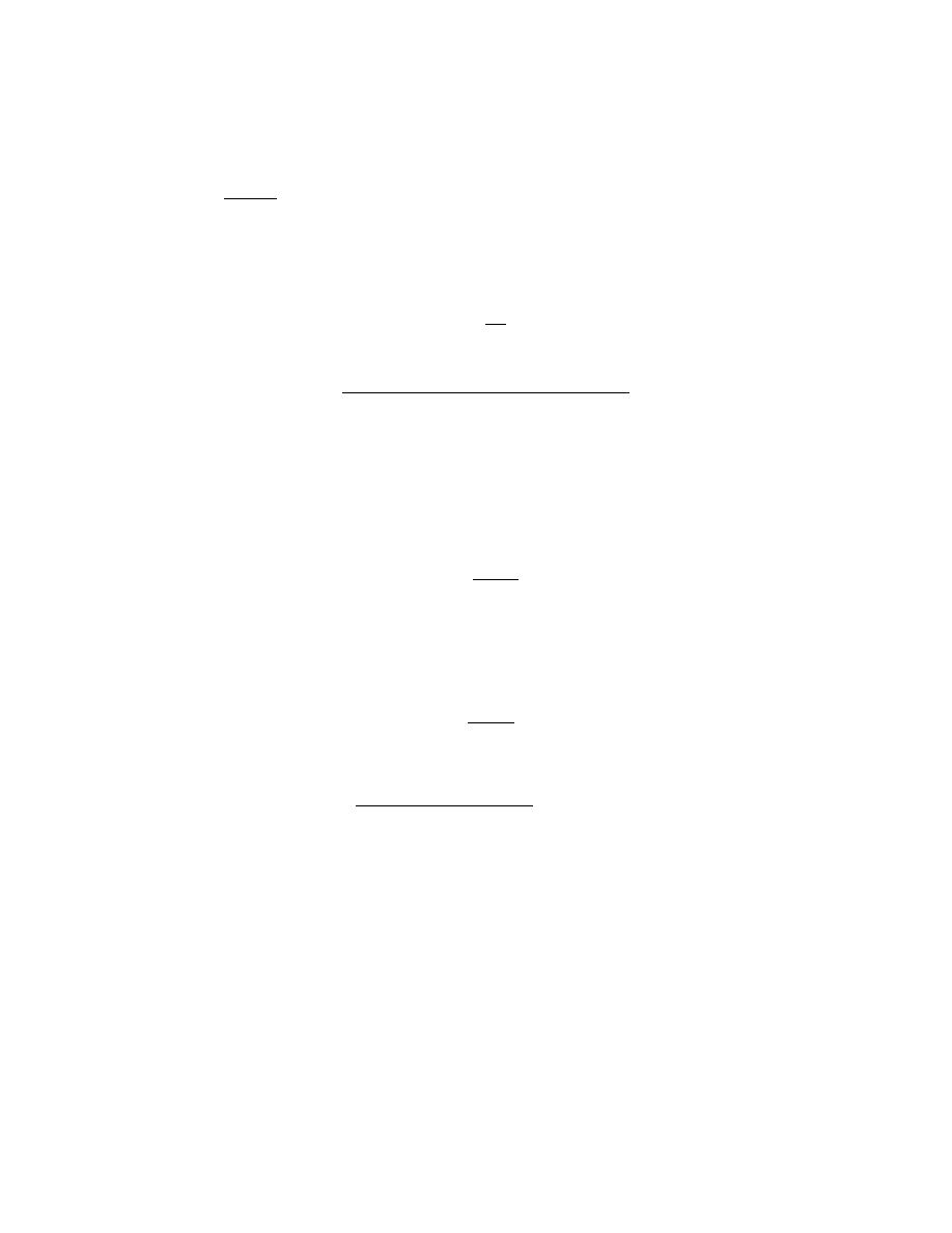
Excerpts from this work may be reproduced by instructors for distribution on a not-for-profit basis for testing or instructional purposes only to
students enrolled in courses for which the textbook has been adopted. Any other reproduction or translation of this work beyond that permitted
by Sections 107 or 108 of the 1976 United States Copyright Act without the permission of the copyright owner is unlawful.
19.5
The constant A in Equation 19.2 is 12π
4
R/5
θ
D
3
, where R is the gas constant and θ
D
is the Debye
temperature (K). Estimate θ
D
for copper, given that the specific heat is 0.78 J/kg-K at 10 K.
Solution
For copper, we want to compute the Debye temperature,
θ
D
, given the expression for A in Equation 19.2
and the heat capacity at 10
K. First of all, let us determine the magnitude of A, as
A =
C
v
T
3
=
(0.78 J/mol - K)(1 kg /1000 g)(63.55 g/mol)
(10 K)
3
= 4.96
× 10
-5
J/mol - K
4
As stipulated in the problem statement
A =
12
π
4
R
5
θ
D
3
Or, solving for
θ
D
θ
D
=
12
π
4
R
5A
1/3
=
(12)(
π)
4
(8.31 J/mol - K)
(5)
(
4.96
× 10
−5
J/mol - K
4
)
1/ 3
= 340 K

Excerpts from this work may be reproduced by instructors for distribution on a not-for-profit basis for testing or instructional purposes only to
students enrolled in courses for which the textbook has been adopted. Any other reproduction or translation of this work beyond that permitted
by Sections 107 or 108 of the 1976 United States Copyright Act without the permission of the copyright owner is unlawful.
19.6 (a) Briefly explain why C
v
rises with increasing temperature at temperatures near 0 K. (b) Briefly
explain why C
v
becomes virtually independent of temperature at temperatures far removed from 0 K.
Solution
(a) The reason that C
v
rises with increasing temperature at temperatures near 0 K is because, in this
temperature range, the allowed vibrational energy levels of the lattice waves are far apart relative to the available
thermal energy, and only a portion of the lattice waves may be excited. As temperature increases, more of the
lattice waves may be excited by the available thermal energy, and, hence, the ability of the solid to absorb energy
(i.e., the magnitude of the heat capacity) increases.
(b) At temperatures far removed from 0 K, C
v
becomes independent of temperature because all of the
lattice waves have been excited and the energy required to produce an incremental temperature change is nearly
constant.

Excerpts from this work may be reproduced by instructors for distribution on a not-for-profit basis for testing or instructional purposes only to
students enrolled in courses for which the textbook has been adopted. Any other reproduction or translation of this work beyond that permitted
by Sections 107 or 108 of the 1976 United States Copyright Act without the permission of the copyright owner is unlawful.
Thermal Expansion
19.7 An aluminum wire 10 m (32.8 ft) long is cooled from 38 to -1°C (100 to 30°F). How much change in
length will it experience?
Solution
In order to determine the change in length of the aluminum wire, we must employ a rearranged form of
Equation 19.3b and using the value of
α
l
taken from Table 19.1 [23.6
× 10
-6
(
°C)
-1
] as
∆l = l
0
α
l
∆T = l
0
α
l
(T
f
− T
0
)
= (10 m) 23.6
× 10
−6
(
°C)
-1
[
]
(
−1°C − 38°C)
=
− 9.2 × 10
-3
m =
− 9.2 mm (−0.36 in.)

Excerpts from this work may be reproduced by instructors for distribution on a not-for-profit basis for testing or instructional purposes only to
students enrolled in courses for which the textbook has been adopted. Any other reproduction or translation of this work beyond that permitted
by Sections 107 or 108 of the 1976 United States Copyright Act without the permission of the copyright owner is unlawful.
19.8 A 0.1 m (3.9 in.) rod of a metal elongates 0.2 mm (0.0079 in.) on heating from 20 to 100°C (68 to
212°F). Determine the value of the linear coefficient of thermal expansion for this material.
Solution
The linear coefficient of thermal expansion for this material may be determined using a rearranged form of
Equation 19.3b as
α
l
=
∆ l
l
0
∆T
=
∆ l
l
0
(T
f
− T
0
)
=
0.2
× 10
−3
m
(0.1 m)(100
°C − 20°C)
= 25.0
× 10
-6
(
°C)
-1

Excerpts from this work may be reproduced by instructors for distribution on a not-for-profit basis for testing or instructional purposes only to
students enrolled in courses for which the textbook has been adopted. Any other reproduction or translation of this work beyond that permitted
by Sections 107 or 108 of the 1976 United States Copyright Act without the permission of the copyright owner is unlawful.
19.9 Briefly explain thermal expansion using the potential energy-versus-interatomic spacing curve.
The phenomenon of thermal expansion using the potential energy-versus-interatomic spacing curve is
explained in Section 19.3.

Excerpts from this work may be reproduced by instructors for distribution on a not-for-profit basis for testing or instructional purposes only to
students enrolled in courses for which the textbook has been adopted. Any other reproduction or translation of this work beyond that permitted
by Sections 107 or 108 of the 1976 United States Copyright Act without the permission of the copyright owner is unlawful.
19.10 Compute the density for nickel at 500°C, given that its room-temperature density is 8.902 g/cm
3
.
Assume that the volume coefficient of thermal expansion, α
v
, is equal to 3α
l
.
Solution
In this problem we are asked to determine the density of nickel at 500
°C. Let us use as the basis for this
determination 1 cm
3
of material at 20
°C, which has a mass of 8.902 g; it is assumed that this mass will remain
constant upon heating to 500
°C. Let us compute the volume expansion of this cubic centimeter of nickel as it is
heated to 500
°C. A volume expansion expression is given in Equation 19.4—viz.,
∆V
V
0
=
α
v
∆T
or
∆V = V
0
α
v
∆T
Also,
α
v
= 3
α
l
, as stipulated in the problem. The value of
α
l
given in Table 19.1 for nickel is 13.3
× 10
-6
(
°C)
-1
.
Therefore, the volume, V, of this specimen of Ni at 500
°C is just
V = V
0
+
∆V = V
0
1
+ α
v
∆T
(
)
= V
0
1
+ 3α
l
∆T
(
)
=
(
1 cm
3
)
1
+ (3) 13.3 × 10
−6
(
°C)
−1
[
]
(500
°C − 20°C)
{
}
= 1.01915 cm
3
Thus, the density is just the 8.902 g divided by this new volume—i.e.,
ρ =
8.902 g
1.01915 cm
3
= 8.735 g/cm
3

Excerpts from this work may be reproduced by instructors for distribution on a not-for-profit basis for testing or instructional purposes only to
students enrolled in courses for which the textbook has been adopted. Any other reproduction or translation of this work beyond that permitted
by Sections 107 or 108 of the 1976 United States Copyright Act without the permission of the copyright owner is unlawful.
19.11 When a metal is heated its density decreases. There are two sources that give rise to this
diminishment of ρ: (1) the thermal expansion of the solid, and (2) the formation of vacancies (Section 4.2). Consider
a specimen of copper at room temperature (20°C) that has a density of 8.940 g/cm
3
. (a) Determine its density upon
heating to 1000°C when only thermal expansion is considered. (b) Repeat the calculation when the introduction of
vacancies is taken into account. Assume that the energy of vacancy formation is 0.90 eV/atom, and that the volume
coefficient of thermal expansion,
α
v
is equal to 3α
l
.
Solution
(a) In this portion of the problem we are asked to determine the density of copper at 1000
°C on the basis
of thermal expansion considerations. The basis for this determination will be 1 cm
3
of material at 20
°C; this
volume of copper has a mass of 8.940 g, which mass is assumed to remain constant upon heating to the 1000
°C.
Let us first compute the volume expansion of this cubic centimeter of copper as it is heated to 1000
°C. According
to Equation 19.4 volume expansion is equal to
∆V
V
0
=
α
v
∆T
where
α
v
, the volume coefficient of thermal expansion, as stipulated in the problem statement, is equal to 3
α
l
. The
value of
α
l
given in Table 19.1 for copper is 17.0
× 10
-6
(
°C)
-1
. Therefore, the volume of this specimen of Cu at
1000
°C (V) is equal to
V = V
0
+
∆V = V
0 +
V
0
α
v
∆T = V
0
(
1
+ α
v
∆T
)
= V
0
(
1
+ 3α
l
∆T
)
= V
0
1
+ 3α
l
(
T
f
− T
0
)
=
(
1 cm
3
)
1
+ (3) 17.0 × 10
−6
(
°C)
−1
[
]
(1000
°C − 20°C)
{
}
= 1.04998 cm
3
Thus, the density is just the 8.940 g divided by this new volume—i.e.,
ρ =
8.940 g
1.04998 cm
3
= 8.514 g/cm
3
(b) Now we are asked to compute the density at 1000
°C taking into consideration the creation of
vacancies which will further lower the density. To begin, this determination requires that we calculate the number

Excerpts from this work may be reproduced by instructors for distribution on a not-for-profit basis for testing or instructional purposes only to
students enrolled in courses for which the textbook has been adopted. Any other reproduction or translation of this work beyond that permitted
by Sections 107 or 108 of the 1976 United States Copyright Act without the permission of the copyright owner is unlawful.
of vacancies using Equation 4.1. But it first becomes necessary to compute the number of Cu atoms per cubic
centimeter (N
Cu
) at 1000
°C using Equation 4.2. Thus,
N
Cu
=
N
A
ρ
Cu
A
Cu
=
(
6.022
× 10
23
atoms / mol
)(
8.514 g/cm
3
)
63.55 g/mol
= 8.07
× 10
22
atoms/cm
3
Now, from Equation 4.1, the total number of vacancies, N
v
, is computed as
N
v
= N
Cu
exp
−
Q
v
kT
=
(
8.07
× 10
22
atoms/cm
3
)
exp
−
0.90 eV / atom
(
8.62
× 10
−5
eV / K
)
(1000
+ 273 K)
= 2.212
× 10
19
vacancies/cm
3
We now want to determine the number of vacancies per unit cell, which is possible if the unit cell volume is
multiplied by N
v
. The unit cell volume (V
C
) may be calculated using Equation 3.5 taking n = 4 inasmuch as Cu has
the FCC crystal structure. Thus, from a rearranged form of Equation 3.5
V
C
=
nA
Cu
ρ
Cu
N
A
=
(4 atoms/unit cell)(63.55 g/mol)
(
8.514 g/cm
3
)(
6.022
× 10
23
atoms / mol
)
= 4.958
× 10
-23
cm
3
/unit cell
Now, the number of vacancies per unit cell, n
v
, is just
n
v
= N
v
V
C
=
(
2.212
× 10
19
vacancies/cm
3
)(
4.958
× 10
-23
cm
3
/unit cell
)

Excerpts from this work may be reproduced by instructors for distribution on a not-for-profit basis for testing or instructional purposes only to
students enrolled in courses for which the textbook has been adopted. Any other reproduction or translation of this work beyond that permitted
by Sections 107 or 108 of the 1976 United States Copyright Act without the permission of the copyright owner is unlawful.
= 0.001097 vacancies/unit cell
What this means is that instead of there being 4.0000 atoms per unit cell, there are only 4.0000 – 0.001097 =
3.998903 atoms per unit cell. And, finally, the density may be computed using Equation 3.5 taking n = 3.998903;
thus
ρ
Cu
=
nA
Cu
V
C
N
A
=
(3.998903 atoms/unit cell)(63.55 g/mol)
(
4.958
× 10
−23
cm
3
/unit cell
)(
6.022
× 10
23
atoms / mol
)
= 8.512 g/cm
3
Thus, the influence of the vacancies is almost insignificant--their presence reduces the density by only 0.002 g/cm
3
(from 8.514 g/cm
3
to 8.512 g/cm
3
).

Excerpts from this work may be reproduced by instructors for distribution on a not-for-profit basis for testing or instructional purposes only to
students enrolled in courses for which the textbook has been adopted. Any other reproduction or translation of this work beyond that permitted
by Sections 107 or 108 of the 1976 United States Copyright Act without the permission of the copyright owner is unlawful.
19.12 The difference between the specific heats at constant pressure and volume is described by the
expression
c
p
− c
v
=
α
v
2
v
0
T
β
(19.10)
where α
v
is the volume coefficient of thermal expansion, v
0
is the specific volume (i.e., volume per unit mass, or the
reciprocal of density), β is the compressibility, and T is the absolute temperature. Compute the values of c
v
at room
temperature (293 K) for copper and nickel using the data in Table 19.1,
assuming that α
v
= 3α
l
and given that the
values of β for Cu and Ni are 8.35 × 10
-12
and 5.51
× 10
-12
(Pa)
-1
, respectively.
Solution
This problem asks that we calculate the values of c
v
for copper and nickel at room temperature using
Equation 19.10, the data in Table 19.1, given that
α
v
= 3
α
l
, and also values of the compressibility. From Equation
19.10
c
v
= c
p
−
α
v
2
v
0
T
β
And, from Table 19.1 and the problem statement
c
p
(Cu) = 386 J/kg-K
c
p
(Ni) = 443 J/kg-K
α
v
(Cu) = (3)[17.0
× 10
-6
(
°C)
-1
] = 5.10
× 10
-5
(
°C)
-1
α
v
(Ni) = (3)[(13.3
× 10
-6
(
°C)
-1
] = 3.99
× 10
-5
(
°C)
-1
β(Cu) = 8.35 × 10
-12
(Pa)
-1
β(Ni) = 5.51 × 10
-12
(Pa)
-1
The specific volume is just the reciprocal of the density; thus, in units of m
3
/kg
v
0
(Cu) =
1
ρ
=
1
8.94 g/cm
3
1000 g
kg
1 m
100 cm
3
= 1.119 × 10
−4
m
3
/kg
v
0
(Ni) =
1
8.90 g/cm
3
1000 g
kg
1 m
100 cm
3
= 1.124 × 10
−4
m
3
/ kg

Excerpts from this work may be reproduced by instructors for distribution on a not-for-profit basis for testing or instructional purposes only to
students enrolled in courses for which the textbook has been adopted. Any other reproduction or translation of this work beyond that permitted
by Sections 107 or 108 of the 1976 United States Copyright Act without the permission of the copyright owner is unlawful.
Therefore, for copper
c
v
(Cu) = c
p
(Cu)
−
α
v
2
(Cu) v
0
(Cu)T
β(Cu)
= 386 J/kg - K
−
5.10
× 10
−5
(
°C)
−1
[
]
2
(
1.119
× 10
−4
m
3
/ kg
)
(293 K)
8.35
× 10
−12
(
N/m
2
)
−1
= 376 J/kg-K
And, also for nickel
c
v
(Ni) = 443 J/kg - K
−
3.99
× 10
−5
(
°C)
−1
[
]
2
(
1.124
× 10
−4
m
3
/ kg
)
(293 K)
5.51
× 10
−12
(
N/m
2
)
−1
= 433 J/kg-K

Excerpts from this work may be reproduced by instructors for distribution on a not-for-profit basis for testing or instructional purposes only to
students enrolled in courses for which the textbook has been adopted. Any other reproduction or translation of this work beyond that permitted
by Sections 107 or 108 of the 1976 United States Copyright Act without the permission of the copyright owner is unlawful.
19.13 To what temperature must a cylindrical rod of tungsten 10.000 mm in diameter and a plate of 316
stainless steel having a circular hole 9.988 mm in diameter have to be heated for the rod to just fit into the hole?
Assume that the initial temperature is 25°C.
Solution
This problem asks for us to determine the temperature to which a cylindrical rod of tungsten 10.000 mm in
diameter must be heated in order for it of just fit into a 9.988 mm diameter circular hole in a plate of 316 stainless
steel, assuming that the initial temperature is 25
°C. This requires the use of Equation 19.3a, which is applied to the
diameters of both the rod and hole. That is
d
f
− d
0
d
0
=
α
l
(
T
f
− T
0
)
Solving this expression for d
f
yields
d
f
= d
0 1 +
α
l
(
T
f
−T
0
)
Now all we need do is to establish expressions for d
f
(316 stainless) and d
f
(W), set them equal to one another, and
solve for T
f
. According to Table 19.1,
α
l
(316 stainless) = 16.0
× 10
-6
(
°C)
-1
and
α
l
(W) = 4.5
× 10
-6
(
°C)
-1
. Thus
d
f
(316 stainless) = d
f
(W)
(9.988 mm) 1
+
{
16.0
× 10
−6
(
°C)
−1
}
(
T
f
− 25°C
)
[
]
= (10.000 mm) 1
+
{
4.5
× 10
−6
(
°C)
−1
}
(
T
f
− 25°C
)
[
]
Now solving for T
f
gives T
f
= 129.5
°C

Excerpts from this work may be reproduced by instructors for distribution on a not-for-profit basis for testing or instructional purposes only to
students enrolled in courses for which the textbook has been adopted. Any other reproduction or translation of this work beyond that permitted
by Sections 107 or 108 of the 1976 United States Copyright Act without the permission of the copyright owner is unlawful.
Thermal Conductivity
19.14 (a) Calculate the heat flux through a sheet of steel 10 mm (0.39 in.) thick if the temperatures at the
two faces are 300 and 100°C (572 and 212°F); assume steady-state heat flow. (b) What is the heat loss per hour if
the area of the sheet is 0.25 m
2
(2.7 ft
2
)? (c) What will be the heat loss per hour if soda–lime glass instead of steel is
used? (d) Calculate the heat loss per hour if steel is used and the thickness is increased to 20 mm (0.79 in.).
Solution
(a) The steady-state heat flux through the plate may be computed using Equation 19.5; the thermal
conductivity for steel, found in Table 19.1, is 51.9 W/m-K. Therefore,
q =
− k
∆T
∆x
=
− (51.9 W/m - K)
(100
+ 273 K) − (300 + 273 K)
10
× 10
−3
m
= 1.04
× 10
6
W/m
2
(b) Let dQ/dt represent the total heat loss such that
dQ
dt
= qAt
where A and t are the cross-sectional area and time, respectively. Thus,
dQ
dt
=
(
1.04
× 10
6
J/s - m
2
)(
0.25 m
2
)
(60 s/min)(60 min/h)
= 9.3
× 10
8
J/h (8.9
× 10
5
Btu/h)
(c) If soda-lime glass is used (k = 1.7 W/m-K, Table 19.1),
dQ
dt
=
− k A t
∆T
∆x
=
− (1.7 J/s - m- K)
(
0.25 m
2
)
(3600 s/h)
− 200 K
10
× 10
−3
m

Excerpts from this work may be reproduced by instructors for distribution on a not-for-profit basis for testing or instructional purposes only to
students enrolled in courses for which the textbook has been adopted. Any other reproduction or translation of this work beyond that permitted
by Sections 107 or 108 of the 1976 United States Copyright Act without the permission of the copyright owner is unlawful.
= 3.06
× 10
7
J/h (2.9
× 10
4
Btu/h)
(d) If the thickness of the steel is increased to 20 mm, then
dQ
dt
=
− k A t
∆T
∆x
= − (51.9 W/m - K)
(
0.25 m
2
)
(3600 s/h)
− 200 K
20
× 10
−3
m
= 4.7
× 10
8
J/h (4.5
× 10
5
Btu/h)

Excerpts from this work may be reproduced by instructors for distribution on a not-for-profit basis for testing or instructional purposes only to
students enrolled in courses for which the textbook has been adopted. Any other reproduction or translation of this work beyond that permitted
by Sections 107 or 108 of the 1976 United States Copyright Act without the permission of the copyright owner is unlawful.
19.15 (a) Would you expect Equation 19.7 to be valid for ceramic and polymeric materials? Why or why
not? (b) Estimate the value for the Wiedemann–Franz constant L
[in Ω-W/(K)
2
] at room temperature (293 K) for
the following nonmetals: silicon (intrinsic), glass-ceramic (Pyroceram), fused silica, polycarbonate, and
polytetrafluoroethylene. Consult Tables B.7 and B.9 in Appendix B.
Solution
(a) Equation 19.7 is not valid for ceramic and polymeric materials since, in the development of this
expression, it is assumed that free electrons are responsible for both electrical and thermal conduction. Such is the
case for most metals. For ceramics and polymers, free electrons are the primary contributors to the electrical
conductivity. However, free electrons do not contribute significantly to the thermal conductivity. For ceramics,
thermal conduction is primarily by means of phonons; for polymers, the energy transfer is made by chain
vibrations, translations, and rotations.
(b) Estimated room-temperature values of L, in
Ω-W/(K)
2
, for the several materials are determined below.
Electrical conductivity values were determined by taking reciprocals of the electrical resistivities given in Table B.9,
Appendix B; thermal conductivities are taken from Table B.7 in the same appendix. (Note: when a range of values
is given in these tables, an average value is used in the computation.)
For intrinsic silicon
L =
k
σT
=
141 W/m - K
1
2500 (
Ω − m)
(293 K)
= 1203
Ω - W/K
2
For Pyroceram glass-ceramic
L =
3.3 W / m - K
1
2
× 10
−14
(
Ω − m)
(293 K)
= 2.3
× 10
12
Ω - W/K
2
For fused silica
L =
1.4 W / m - K
1
10
18
(
Ω − m)
(293 K)
= 4.8
× 10
15
Ω - W/K
2
For polycarbonate

Excerpts from this work may be reproduced by instructors for distribution on a not-for-profit basis for testing or instructional purposes only to
students enrolled in courses for which the textbook has been adopted. Any other reproduction or translation of this work beyond that permitted
by Sections 107 or 108 of the 1976 United States Copyright Act without the permission of the copyright owner is unlawful.
L =
0.20 W / m - K
1
2
× 10
14
(
Ω − m)
(293 K)
= 1.4
× 10
11
Ω - W/K
2
For polytetrafluoroethylene
L =
0.25 W / m - K
1
10
17
(
Ω − m)
(293 K)
= 8.5
× 10
13
Ω - W/K
2

Excerpts from this work may be reproduced by instructors for distribution on a not-for-profit basis for testing or instructional purposes only to
students enrolled in courses for which the textbook has been adopted. Any other reproduction or translation of this work beyond that permitted
by Sections 107 or 108 of the 1976 United States Copyright Act without the permission of the copyright owner is unlawful.
19.16 Briefly explain why the thermal conductivities are higher for crystalline than noncrystalline
ceramics.
Solution
Thermal conductivities are higher for crystalline than for noncrystalline ceramics because, for
noncrystalline, phonon scattering, and thus the resistance to heat transport, is much more effective due to the highly
disordered and irregular atomic structure.

Excerpts from this work may be reproduced by instructors for distribution on a not-for-profit basis for testing or instructional purposes only to
students enrolled in courses for which the textbook has been adopted. Any other reproduction or translation of this work beyond that permitted
by Sections 107 or 108 of the 1976 United States Copyright Act without the permission of the copyright owner is unlawful.
19.17 Briefly explain why metals are typically better thermal conductors than ceramic materials.
Solution
Metals are typically better thermal conductors than are ceramic materials because, for metals, most of the
heat is transported by free electrons (of which there are relatively large numbers). In ceramic materials, the primary
mode of thermal conduction is via phonons, and phonons are more easily scattered than are free electrons.

Excerpts from this work may be reproduced by instructors for distribution on a not-for-profit basis for testing or instructional purposes only to
students enrolled in courses for which the textbook has been adopted. Any other reproduction or translation of this work beyond that permitted
by Sections 107 or 108 of the 1976 United States Copyright Act without the permission of the copyright owner is unlawful.
19.18 (a) Briefly explain why porosity decreases the thermal conductivity of ceramic and polymeric
materials, rendering them more thermally insulative. (b) Briefly explain how the degree of crystallinity affects the
thermal conductivity of polymeric materials and why.
Solution
(a) Porosity decreases the thermal conductivity of ceramic and polymeric materials because the thermal
conductivity of a gas phase that occupies pore space is extremely small relative to that of the solid material.
Furthermore, contributions from gaseous convection are generally insignificant.
(b) Increasing the degree of crystallinity of a semicrystalline polymer enhances its thermal conductivity;
the vibrations, rotations, etc. of the molecular chains are more effective modes of thermal transport when a
crystalline structure prevails.

Excerpts from this work may be reproduced by instructors for distribution on a not-for-profit basis for testing or instructional purposes only to
students enrolled in courses for which the textbook has been adopted. Any other reproduction or translation of this work beyond that permitted
by Sections 107 or 108 of the 1976 United States Copyright Act without the permission of the copyright owner is unlawful.
19.19 For some ceramic materials, why does the thermal conductivity first decrease and then increase
with rising temperature?
Solution
For some ceramic materials, the thermal conductivity first decreases with rising temperature because the
scattering of lattice vibrations increases with temperature. At higher temperatures, the thermal conductivity will
increase for some ceramics that are porous because radiant heat transfer across pores may become important, which
process increases with rising temperature.

Excerpts from this work may be reproduced by instructors for distribution on a not-for-profit basis for testing or instructional purposes only to
students enrolled in courses for which the textbook has been adopted. Any other reproduction or translation of this work beyond that permitted
by Sections 107 or 108 of the 1976 United States Copyright Act without the permission of the copyright owner is unlawful.
19.20 For each of the following pairs of materials, decide which has the larger thermal conductivity.
Justify your choices.
(a) Pure copper; aluminum bronze (95 wt% Cu-5 wt% Al).
(b) Fused silica; quartz.
(c) Linear polyethylene; branched polyethylene.
(d) Random poly(styrene-butadiene) copolymer; alternating poly(styrene-butadiene) copolymer.
Solution
This question asks for us to decide, for each of several pairs of materials, which has the larger thermal
conductivity and why.
(a) Pure copper will have a larger conductivity than aluminum bronze because the impurity atoms in the
latter will lead to a greater degree of free electron scattering.
(b) Quartz will have a larger conductivity than fused silica because fused silica is noncrystalline (whereas
quartz is crystalline) and lattice vibrations are more effectively scattered in noncrystalline materials.
(c) The linear polyethylene will have the larger conductivity than the branched polyethylene because the
former will have the higher degree of crystallinity. Linear polymers have higher degrees of crystallinity than
branched polymers. Since heat transfer is accomplished by molecular chain vibrations, and the coordination of
these vibrations increases with percent crystallinity, the higher the crystallinity, the greater the thermal conductivity.
(d) The alternating poly(styrene-butadiene) copolymer will have a higher crystallinity than the random
copolymer; alternating copolymers crystallize more easily than random ones. The influence of crystallinity on
conductivity is explained in part (c).

Excerpts from this work may be reproduced by instructors for distribution on a not-for-profit basis for testing or instructional purposes only to
students enrolled in courses for which the textbook has been adopted. Any other reproduction or translation of this work beyond that permitted
by Sections 107 or 108 of the 1976 United States Copyright Act without the permission of the copyright owner is unlawful.
19.21 We might think of a porous material as being a composite wherein one of the phases is a pore
phase. Estimate upper and lower limits for the room-temperature thermal conductivity of a magnesium oxide
material having a volume fraction of 0.30 of pores that are filled with still air.
Solution
This problem asks that we treat a porous material as a composite wherein one of the phases is a pore phase,
and that we estimate upper and lower limits for the room-temperature thermal conductivity of a magnesium oxide
material having a 0.30 volume fraction of pores. The upper limit of k
(
k
upper
)
may be determined using Equation
16.1 with thermal conductivity substituted for the elastic modulus, E. From Table 19.1, the value of k for MgO is
37.7 W/m-K, while for still air in the pore phase, k = 0.02 W/m-K (Section 19.4). Thus
k
upper
= V
p
k
air
+ V
MgO
k
MgO
= (0.30)(0.02 W/m-K) + (0.70)(37.7 W/m-K) = 26.4 W/m-K
For the lower limit we employ a modification of Equation 16.2 as
k
lower
=
k
air
k
MgO
V
p
k
MgO
+ V
MgO
k
air
=
(0.02 W/m - K)(37.7 W / m - K)
(0.30)(37.7 W / m - K)
+ (0.70)(0.02 W /m- K)
= 0.067 W/m - K

Excerpts from this work may be reproduced by instructors for distribution on a not-for-profit basis for testing or instructional purposes only to
students enrolled in courses for which the textbook has been adopted. Any other reproduction or translation of this work beyond that permitted
by Sections 107 or 108 of the 1976 United States Copyright Act without the permission of the copyright owner is unlawful.
19.22 Nonsteady-state heat flow may be described by the following partial differential equation:
∂T
∂t
= D
T
∂
2
T
∂x
2
where D
T
is the thermal diffusivity; this expression is the thermal equivalent of Fick’s second law of diffusion
(Equation 5.4b). The thermal diffusivity is defined according to
D
T
=
k
ρc
p
In this expression, k,
ρ, and c
p
represent the thermal conductivity, the mass density, and the specific heat at constant
pressure, respectively.
(a) What are the SI units for D
T
?
(b) Determine values of D
T
for aluminum, steel, aluminum oxide, soda–lime glass, polystyrene, and nylon
6,6 using the data in Table 19.1. Density values are included in Table B.1, Appendix B.
Solution
(a) The units of D
T
are
D
T
=
k (J /s - m - K)
ρ
(
kg / m
3
)
c
p
(J / kg - K)
= m
2
/s
(b) The values of D
T
for the several materials are given below. (Note: values for k and c
p
are taken from
Table 19.1; density values are from Table B.1, Appendix B, and converted to units of kilograms per meter cubed):
For aluminum
D
T
=
k
ρ c
p
=
247 W/m - K
(
2.71
× 10
3
kg/m
3
)
(900 J/kg - K)
= 1.0
× 10
-4
m
2
/s
For steel
D
T
=
51.9 W/m - K
(
7.9
× 10
3
kg/m
3
)
(486 J/kg - K)
= 1.4
× 10
-5
m
2
/s
For aluminum oxide

Excerpts from this work may be reproduced by instructors for distribution on a not-for-profit basis for testing or instructional purposes only to
students enrolled in courses for which the textbook has been adopted. Any other reproduction or translation of this work beyond that permitted
by Sections 107 or 108 of the 1976 United States Copyright Act without the permission of the copyright owner is unlawful.
D
T
=
39 W/m - K
(
4
× 10
3
kg/m
3
)
(775 J/kg - K)
= 1.26
× 10
-5
m
2
/s
For soda-lime glass
D
T
=
1.7 W/m - K
(
2.5
× 10
3
kg/m
3
)
(840 J/kg - K)
= 8.1
× 10
-7
m
2
/s
For polystyrene
D
T
=
0.13 W/m - K
(
1.05
× 10
3
kg/m
3
)
(1170 J/kg - K)
= 1.06
× 10
-7
m
2
/s
For nylon 6,6
D
T
=
0.24 W/m - K
(
1.14
× 10
3
kg/m
3
)
(1670 J/kg - K)
= 1.3
× 10
-7
m
2
/s
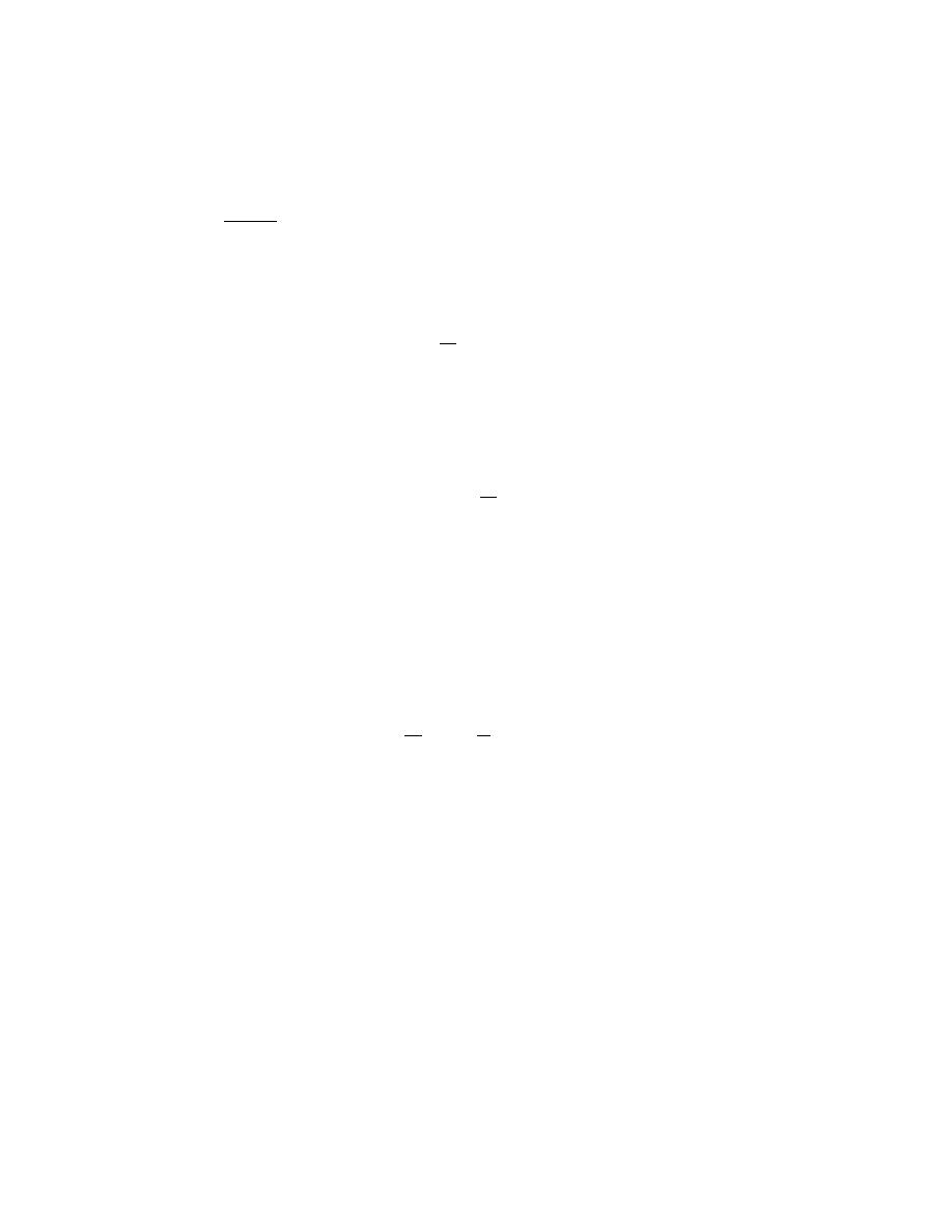
Excerpts from this work may be reproduced by instructors for distribution on a not-for-profit basis for testing or instructional purposes only to
students enrolled in courses for which the textbook has been adopted. Any other reproduction or translation of this work beyond that permitted
by Sections 107 or 108 of the 1976 United States Copyright Act without the permission of the copyright owner is unlawful.
Thermal Stresses
19.23 Beginning with Equation 19.3, show that Equation 19.8 is valid.
Solution
We want to show that Equation 19.8 is valid beginning with Equation 19.3. Upon examination of Equation
19.3b,
∆l
l
0
=
α
l
∆T
it may be noted that the term on the left-hand side is the same expression as that for the definition of engineering
strain (Equation 6.2); that is
ε =
∆l
l
0
Furthermore, elastic stress and strain are related through Hooke's law, Equation 6.5:
σ = Eε
Making appropriate substitutions and algebraic manipulations gives
∆l
l
0
=
ε =
σ
E
=
α
l
∆T
Or, solving for
σ
σ = Eα
l
∆T
which is the form of Equation 19.8.

Excerpts from this work may be reproduced by instructors for distribution on a not-for-profit basis for testing or instructional purposes only to
students enrolled in courses for which the textbook has been adopted. Any other reproduction or translation of this work beyond that permitted
by Sections 107 or 108 of the 1976 United States Copyright Act without the permission of the copyright owner is unlawful.
19.24 (a) Briefly explain why thermal stresses may be introduced into a structure by rapid heating or
cooling. (b) For cooling, what is the nature of the surface stresses? (c) For heating, what is the nature of the
surface stresses?
Solution
(a) Thermal stresses may be introduced into a structure by rapid heating or cooling because temperature
gradients will be established across the cross section due to more rapid temperature changes at the surface than
within the interior; thus, the surface will expand or contract at a different rate than the interior and since this surface
expansion or contraction will be restrained by the interior, stresses will be introduced.
(b) For cooling, the surface stresses will be tensile in nature since the interior contracts to a lesser degree
than the cooler surface.
(c) For heating, the surface stresses will be compressive in nature since the interior expands to a lesser
degree than the hotter surface.

Excerpts from this work may be reproduced by instructors for distribution on a not-for-profit basis for testing or instructional purposes only to
students enrolled in courses for which the textbook has been adopted. Any other reproduction or translation of this work beyond that permitted
by Sections 107 or 108 of the 1976 United States Copyright Act without the permission of the copyright owner is unlawful.
19.25 (a) If a rod of 1025 steel 0.5 m (19.7 in.) long is heated from 20 to 80°C (68 to 176°F) while its ends
are maintained rigid, determine the type and magnitude of stress that develops. Assume that at 20°C the rod is
stress free. (b) What will be the stress magnitude if a rod 1 m (39.4 in.) long is used? (c) If the rod in part (a) is
cooled from 20 to -10°C (68 to 14°F), what type and magnitude of stress will result?
Solution
(a) We are asked to compute the magnitude of the stress within a 1025 steel rod that is heated while its
ends are maintained rigid. To do this we employ Equation 19.8, using a value of 207 GPa for the modulus of
elasticity of steel (Table 6.1), and a value of 12.0
× 10
-6
(
°C)
-1
for
α
l
(Table 19.1). Therefore
σ = Eα
l
(
T
0
− T
f
)
=
(
207
× 10
3
MPa
)
12.0
× 10
−6
(
°C)
−1
[
]
(20
°C − 80°C)
= –150 MPa (–21,800 psi)
The stress will be compressive since its sign is negative.
(b) The stress will be the same [–150 MPa (–21,800 psi )], since stress is independent of bar length.
(c) Upon cooling the indicated amount, the stress becomes
σ = Eα
l
(
T
0
− T
f
)
=
(
207
× 10
3
MPa
)
12.0
× 10
−6
(
°C)
−1
[
]
(20
°C − (−10°C)
[
]
= +74.5 MPa (+10,900 psi)
This stress will be tensile since its sign is positive.

Excerpts from this work may be reproduced by instructors for distribution on a not-for-profit basis for testing or instructional purposes only to
students enrolled in courses for which the textbook has been adopted. Any other reproduction or translation of this work beyond that permitted
by Sections 107 or 108 of the 1976 United States Copyright Act without the permission of the copyright owner is unlawful.
19.26 A copper wire is stretched with a stress of 70 MPa (10,000 psi) at 20°C (68°F). If the length is held
constant, to what temperature must the wire be heated to reduce the stress to 35 MPa (5000 psi)?
Solution
We want to heat the copper wire in order to reduce the stress level from 70 MPa to 35 MPa; in doing so,
we reduce the stress in the wire by 70 MPa – 35 MPa = 35 MPa, which stress will be a compressive one (i.e.,
σ = –
35 MPa). Solving for T
f
from Equation 19.8 [and using values for E and
α
l
of 110 GPa (Table 6.1) and 17.0
× 10
-6
(
°C)
-1
(Table 19.1), respectively] yields
T
f
= T
0
−
σ
E
α
l
= 20
°C −
− 35 MPa
(
110
× 10
3
MPa
)
17.0
× 10
−6
(
°C)
−1
[
]
= 20
°C + 19°C = 39°C (101°F)

Excerpts from this work may be reproduced by instructors for distribution on a not-for-profit basis for testing or instructional purposes only to
students enrolled in courses for which the textbook has been adopted. Any other reproduction or translation of this work beyond that permitted
by Sections 107 or 108 of the 1976 United States Copyright Act without the permission of the copyright owner is unlawful.
19.27 If a cylindrical rod of nickel 100.00 mm long and 8.000 mm in diameter is heated from 20
°C to
200
°C while its ends are maintained rigid, determine its change in diameter. You may want to consult Table 6.1.
Solution
This problem asks for us to determine the change in diameter of a cylindrical nickel rod 100.00 mm long
and 8.000 mm in diameter when it is heated from 20
°C to 200°C while its ends are maintained rigid. There will be
two contributions to the diameter increase of the rod; the first is due to thermal expansion (which will be denoted as
∆d
1
), while the second is from Poisson's lateral expansion as a result of elastic deformation from stresses that are
established from the inability of the rod to elongate as it is heated (denoted as
∆d
2
). The magnitude of
∆d
1
may be
computed using a modified form of Equation 19.3 as
∆d
1
= d
0
α
l
(
T
f
− T
0
)
From Table 19.1 the value of
α
l
for nickel is 13.3
× 10
-6
(
°C)
-1
. Thus,
∆d
1
= (8.000 mm) 13.3
× 10
−6
(
°C)
−1
[
]
(200
°C − 20°C)
= 0.0192 mm
Now,
∆d
2
is related to the transverse strain (
ε
x
) according to a modified form of Equation 6.2 as
∆d
2
d
0
=
ε
x
Also, transverse strain and longitudinal strain (
ε
z
) are related according to Equation 6.8:
ε
x
= − νε
z
where
ν is Poisson’s ratio. Substitution of this expression for ε
x
into the first equation above leads to
∆d
2
d
0
=
− νε
z
Furthermore, the longitudinal strain is related to the modulus of elasticity through Equation 6.5—i.e.,

Excerpts from this work may be reproduced by instructors for distribution on a not-for-profit basis for testing or instructional purposes only to
students enrolled in courses for which the textbook has been adopted. Any other reproduction or translation of this work beyond that permitted
by Sections 107 or 108 of the 1976 United States Copyright Act without the permission of the copyright owner is unlawful.
ε
z
=
σ
E
And, therefore,
∆d
2
d
0
=
− ν
σ
E
Now, from Equation 19.8 stress is equal to
σ = Eα
l
(
T
0
− T
f
)
which, when substituted into the preceding equation leads to
∆d
2
d
0
=
−
νEα
l
(
T
0
− T
f
)
E
=
− να
l
(
T
0
− T
f
)
Solving for
∆d
2
and realizing that, for nickel,
ν = 0.31 (Table 6.1) yields
∆d
2
=
− d
0
να
l
(
T
0
− T
f
)
=
− (8.000 mm)(0.31) 13.3 × 10
−6
(
°C)
−1
[
]
(20
°C − 200°C)
= 0.0059 mm
Finally, the total
∆d is just ∆d
1
+
∆d
2
= 0.0192 mm + 0.0059 mm = 0.0251 mm.

Excerpts from this work may be reproduced by instructors for distribution on a not-for-profit basis for testing or instructional purposes only to
students enrolled in courses for which the textbook has been adopted. Any other reproduction or translation of this work beyond that permitted
by Sections 107 or 108 of the 1976 United States Copyright Act without the permission of the copyright owner is unlawful.
19.28 The two ends of a cylindrical rod of 1025 steel 75.00 mm long and 10.000 mm in diameter are
maintained rigid. If the rod is initially at 25
°C, to what temperature must it be cooled to have a 0.008-mm
reduction in diameter?
Solution
This problem asks for us to determine to what temperature a cylindrical rod of 1025 steel 75.00 mm long
and 10.000 mm in diameter must be cooled from 25
°C in order to have a 0.008 mm reduction in diameter if the rod
ends are maintained rigid. There will be two contributions to the diameter decrease of the rod; the first is due to
thermal contraction (which will be denoted as
∆d
1
), while the second is from Poisson's lateral contraction as a result
of elastic deformation from stresses that are established from the inability of the rod to contract as it is cooled
(denoted as
∆d
2
). The magnitude of
∆d
1
may be computed using a modified form of Equation 19.3b as
∆d
1
= d
0
α
l
(
T
f
− T
0
)
Now,
∆d
2
is related to the transverse strain (
ε
x
) according to a modified form of Equation 6.2 as
∆d
2
d
0
=
ε
x
Also, transverse strain and longitudinal strain (
ε
z
) are related according to Equation 6.8:
ε
x
= − νε
z
where
ν is Poisson’s ratio. Substitution of this expression for ε
x
into the first equation above leads to
∆d
2
d
0
=
− νε
z
Furthermore, the longitudinal strain is related to the modulus of elasticity through Equation 6.5—i.e.,
ε
z
=
σ
E
And, therefore,
∆d
2
d
0
=
− ν
σ
E

Excerpts from this work may be reproduced by instructors for distribution on a not-for-profit basis for testing or instructional purposes only to
students enrolled in courses for which the textbook has been adopted. Any other reproduction or translation of this work beyond that permitted
by Sections 107 or 108 of the 1976 United States Copyright Act without the permission of the copyright owner is unlawful.
Now, from Equation 19.8 stress is equal to
σ = Eα
l
(
T
0
− T
f
)
which, when substituted into the preceding equation leads to
∆d
2
d
0
=
−
νEα
l
(
T
0
− T
f
)
E
=
− να
l
(
T
0
− T
f
)
And, solving for
∆d
2
from this expression
∆d
2
=
− d
0
να
l
(
T
0
− T
f
)
The total
∆d is just ∆d = ∆d
1
+
∆d
2
, and
∆d = d
0
α
l
(
T
f
− T
0
)
+ d
0
να
l
(
T
f
− T
0
)
= d
0
α
l
(
T
f
− T
0
)
(1 +
ν)
The values of
ν and α
l
for 1025 steel are 0.30 and 12.0
× 10
-6
(
°C)
-1
, respectively (Tables 6.1 and 19.1).
Incorporating, into the above equation, these values, as well as those for
∆d, d
0
, and T
0
cited in the problem
statement gives
− (0.008 mm) = (10.000 mm) 12.0 × 10
−6
(
°C)
−1
[
]
(
T
f
− 25°C
)
(1
+ 0.30)
And, finally, solving the above expression for T
f
yields T
f
= – 26.3
°C.

Excerpts from this work may be reproduced by instructors for distribution on a not-for-profit basis for testing or instructional purposes only to
students enrolled in courses for which the textbook has been adopted. Any other reproduction or translation of this work beyond that permitted
by Sections 107 or 108 of the 1976 United States Copyright Act without the permission of the copyright owner is unlawful.
19.29 What measures may be taken to reduce the likelihood of thermal shock of a ceramic piece?
Solution
According to Equation 19.9, the thermal shock resistance of a ceramic piece may be enhanced by
increasing the fracture strength and thermal conductivity, and by decreasing the elastic modulus and linear
coefficient of thermal expansion. Of these parameters,
σ
f
and
α
l
are most amenable to alteration, usually be
changing the composition and/or the microstructure.

Excerpts from this work may be reproduced by instructors for distribution on a not-for-profit basis for testing or instructional purposes only to
students enrolled in courses for which the textbook has been adopted. Any other reproduction or translation of this work beyond that permitted
by Sections 107 or 108 of the 1976 United States Copyright Act without the permission of the copyright owner is unlawful.
DESIGN PROBLEMS
Thermal Expansion
19.D1 Railroad tracks made of 1025 steel are to be laid during the time of year when the temperature
averages 10°C (50°F). If a joint space of 4.6 mm (0.180 in.) is allowed between the standard 11.9-m (39-ft) long
rails, what is the hottest possible temperature that can be tolerated without the introduction of thermal stresses?
Solution
For these railroad tracks, each end is allowed to expand one-half of the joint space distance, or the track
may expand a total of this distance (4.6 mm). Equation 19.3a is used to solve for T
f
, where the value
α
l
for the 1025
steel [12.0
× 10
-6
(
°C)
-1
] is found in Table 19.1. Thus, solving for T
f
from Equation 19.3a leads to
T
f
=
∆ l
α
l
l
0
+ T
0
=
4.6
× 10
−3
m
12.0
× 10
−6
(
°C)
−1
[
]
(11.9 m)
+ 10
°C
= 32.2
°C + 10°C = 42.2°C (108°F)

Excerpts from this work may be reproduced by instructors for distribution on a not-for-profit basis for testing or instructional purposes only to
students enrolled in courses for which the textbook has been adopted. Any other reproduction or translation of this work beyond that permitted
by Sections 107 or 108 of the 1976 United States Copyright Act without the permission of the copyright owner is unlawful.
Thermal Stresses
19.D2 The ends of a cylindrical rod 6.4 mm (0.25 in.) in diameter and 250 mm (10 in.) long are mounted
between rigid supports. The rod is stress free at room temperature [20
°C (68°F)]; and upon cooling to -40°C (-
40
°F), a maximum thermally induced tensile stress of 125 MPa (18,125 psi) is possible. Of which of the following
metals or alloys may the rod be fabricated: aluminum, copper, brass, 1025 steel, and tungsten? Why?
Solution
This is really a materials selection problem in which we must decide for which of the five metals listed, the
stress in the rod will not exceed 125 MPa (18,125 psi), when it is heated while its ends are mounted in rigid
supports. Upon examination of Equation 19.8, it may be noted that all we need do is to compute the E
α
l
∆T product
for each of the candidate materials, and then note for which of them the stress is less than the stipulated maximum.
[The value of
∆T is T
0
– T
f
= 20
°C – (–40°C) = 60°C.] These parameters and their product for each of the alloys
are tabulated below. (Modulus of elasticity values were taken from Table 6.1, while the
α
l
values came from Table
19.1.)
Alloy
α
l
(
°C)
-1
E (MPa)
α
l
E
∆T (MPa)
Aluminum
23.6
× 10
-6
69
× 10
3
98
Copper
17.0
× 10
-6
110
× 10
3
112
Brass
20.0
× 10
-6
97
× 10
3
116
1025 Steel
12.0
× 10
-6
207
× 10
3
149
Tungsten
4.5
× 10
-6
407
× 10
3
110
Thus, aluminum, copper, brass, and tungsten are suitable candidates.

Excerpts from this work may be reproduced by instructors for distribution on a not-for-profit basis for testing or instructional purposes only to
students enrolled in courses for which the textbook has been adopted. Any other reproduction or translation of this work beyond that permitted
by Sections 107 or 108 of the 1976 United States Copyright Act without the permission of the copyright owner is unlawful.
19.D3 (a) What are the units for the thermal shock resistance parameter (TSR)? (b) Rank the following
ceramic materials according to their thermal shock resistance: glass-ceramic (Pyroceram), partially stabilized
zirconia, and borosilicate (Pyrex) glass. Appropriate data may be found in Tables B.2, B.4, B.6, and B.7 of
Appendix B.
Solution
(a) This portion of the problem asks that we cite the units for the thermal shock resistance parameter
(TSR). From Equation 19.9
TSR =
σ
f
(
N / m
2
)
k (W / m - K)
E
(
N / m
2
)
α
l
(
°C)
−1
= W /m
(Note: in reducing units in the above expression, we have assumed that units of temperature in K and
°C are
equivalent)
(b) Now we are asked to rank glass-ceramic (Pyroceram), partially-stabilized zirconia, and borosilicate
(Pyrex) glass as to their thermal shock resistance. Thus, all we need do is calculate, for each, the value of TSR using
Equation 19.9. Values of E,
σ
f
,
α
l
, and k are found, respectively, in Tables B.2, B.4, B.6, and B.7, Appendix B.
(Note: whenever a range for a property value in these tables is cited, the average of the extremes is used.)
For the glass-ceramic
TSR =
σ
f
k
E
α
l
=
(247 MPa)(3.3 W/m - K)
(
120
× 10
3
MPa
)
6.5
× 10
−6
(
°C)
−1
[
]
= 1045 W/m
For partially-stabilized zirconia
TSR =
(1150 MPa)(2.7 W/m - K)
(
205
× 10
3
MPa
)
9.6
× 10
−6
(
°C)
−1
[
]
= 1578 W/m
And, for borosilicate glass
TSR =
(69 MPa)(1.4 W/m - K)
(
70
× 10
3
MPa
)
3.3
× 10
−6
(
°C)
−1
[
]
= 418 W/m

Excerpts from this work may be reproduced by instructors for distribution on a not-for-profit basis for testing or instructional purposes only to
students enrolled in courses for which the textbook has been adopted. Any other reproduction or translation of this work beyond that permitted
by Sections 107 or 108 of the 1976 United States Copyright Act without the permission of the copyright owner is unlawful.
Thus, these materials may be ranked according to their thermal shock resistance from the greatest to the
least as follows: partially-stabilized zirconia, glass-ceramic, and borosilicate glass.

Excerpts from this work may be reproduced by instructors for distribution on a not-for-profit basis for testing or instructional purposes only to
students enrolled in courses for which the textbook has been adopted. Any other reproduction or translation of this work beyond that permitted
by Sections 107 or 108 of the 1976 United States Copyright Act without the permission of the copyright owner is unlawful.
19.D4 Equation 19.9, for the thermal shock resistance of a material, is valid for relatively low rates of
heat transfer. When the rate is high, then, upon cooling of a body, the maximum temperature change allowable
without therm
al shock, ΔT
f
, is approximately
∆T
f
=
σ
f
E
α
l
where σ
f
is the fracture strength. Using the data in Tables B.2, B.4, and B.6 (Appendix B), determine ΔT
f
for a
glass-ceramic (Pyroceram), partially stabilized zirconia, and fused silica.
Solution
We want to compute the maximum temperature change allowable without thermal shock for these three
ceramic materials, which temperature change is a function of the fracture strength, elastic modulus, and linear
coefficient of thermal expansion. These data and the
∆T
f
's are tabulated below. (Values for E,
σ
f
, and
α
l
are taken
from Tables B.2, B.4, B.6 in Appendix B.)
Material
σ
f
(MPa)
E (MPa)
α
l
(
°C)
-1
∆T
f
(
°C)
Glass ceramic
247
120
× 10
3
6.5
× 10
-6
317
Zirconia
1150
205
× 10
3
9.6
× 10
-6
584
Fused silica
104
73
× 10
3
0.4
× 10
-6
3562

Excerpts from this work may be reproduced by instructors for distribution on a not-for-profit basis for testing or instructional purposes only to
students enrolled in courses for which the textbook has been adopted. Any other reproduction or translation of this work beyond that permitted
by Sections 107 or 108 of the 1976 United States Copyright Act without the permission of the copyright owner is unlawful.
CHAPTER 20
MAGNETIC PROPERTIES
PROBLEM SOLUTIONS
Basic Concepts
20.1 A coil of wire 0.20 m long and having 200 turns carries a current of 10 A.
(a) What is the magnitude of the magnetic field strength H?
(b) Compute the flux density B if the coil is in a vacuum.
(c) Compute the flux density inside a bar of titanium that is positioned within the coil. The susceptibility for
titanium is found in Table 20.2.
(d) Compute the magnitude of the magnetization M.
Solution
(a) We may calculate the magnetic field strength generated by this coil using Equation 20.1 as
H =
NI
l
=
(200 turns)(10 A)
0.20 m
= 10, 000 A - turns/m
(b) In a vacuum, the flux density is determined from Equation 20.3. Thus,
B
0
=
µ
0
H
=
(
1.257
× 10
-6
H/m
)
(10,000 A - turns/m) = 1.257
× 10
-2
tesla
(c) When a bar of titanium is positioned within the coil, we must use an expression that is a combination
of Equations 20.5 and 20.6 in order to compute the flux density given the magnetic susceptibility. Inasmuch as
χ
m
= 1.81
× 10
-4
(Table 20.2), then
B =
µ
0
H +
µ
0
M =
µ
0
H +
µ
0
χ
m
H =
µ
0
H
(
1 +
χ
m
)
=
(
1.257
× 10
-6
H/m
)
(10,000 A - turns/m)
(
1 + 1.81
× 10
-4
)

Excerpts from this work may be reproduced by instructors for distribution on a not-for-profit basis for testing or instructional purposes only to
students enrolled in courses for which the textbook has been adopted. Any other reproduction or translation of this work beyond that permitted
by Sections 107 or 108 of the 1976 United States Copyright Act without the permission of the copyright owner is unlawful.
= 1.257 × 10
-2
tesla
which is essentially the same result as part (b). This is to say that the influence of the titanium bar within the coil
makes an imperceptible difference in the magnitude of the B field.
(d) The magnetization is computed from Equation 20.6:
M =
χ
m
H =
(
1.81
× 10
-4
)
(10,000 A - turns/m) = 1.81 A/m

Excerpts from this work may be reproduced by instructors for distribution on a not-for-profit basis for testing or instructional purposes only to
students enrolled in courses for which the textbook has been adopted. Any other reproduction or translation of this work beyond that permitted
by Sections 107 or 108 of the 1976 United States Copyright Act without the permission of the copyright owner is unlawful.
20.2 Demonstrate that the relative permeability and the magnetic susceptibility are related according to
Equation 20.7.
Solution
This problem asks us to show that
χ
m
and
µ
r
are related according to
χ
m
=
µ
r
– 1. We begin with Equation
20.5 and substitute for M using Equation 20.6. Thus,
B =
µ
0
H +
µ
0
M =
µ
0
H +
µ
0
χ
m
H
But B is also defined in Equation 20.2 as
B =
µH
When the above two expressions are set equal to one another as
µH = µ
0
H +
µ
0
χ
m
H
This leads to
µ = µ
0
(
1 +
χ
m
)
If we divide both sides of this expression by
µ
0
, and from the definition of
µ
r
(Equation 20.4), then
µ
µ
0
=
µ
r
= 1 +
χ
m
or, upon rearrangement
χ
m
=
µ
r
−1
which is the desired result.

Excerpts from this work may be reproduced by instructors for distribution on a not-for-profit basis for testing or instructional purposes only to
students enrolled in courses for which the textbook has been adopted. Any other reproduction or translation of this work beyond that permitted
by Sections 107 or 108 of the 1976 United States Copyright Act without the permission of the copyright owner is unlawful.
20.3
It is possible to express the magnetic susceptibility χ
m
in several different units. For the discussion of
this chapter, χ
m
was used to designate the volume susceptibility in SI units, that is, the quantity that gives the
magnetization per unit volume (m
3
) of material when multiplied by H. The mass susceptibility χ
m
(kg) yields the
magnetic moment (or magnetization) per kilogram of material when multiplied by H; and, similarly, the atomic
susceptibility χ
m
(a) gives the magnetization per kilogram-
mole. The latter two quantities are related to χ
m
through
the relationships
χ
m
= χ
m
(kg) × mass density (in kg/m
3
)
χ
m
(a)
= χ
m
(kg) × atomic weight (in kg)]
When using the cgs–emu system, comparable parameters exist, w
hich may be designated by χ′
m
, χ′
m
(g), and χ′
m
(a);
the χ
m
and χ′
m
are related in accordance with Table 20.1. From Table 20.2, χ
m
for silver is –2.38 × 10
–5
; convert
this value into the other five susceptibilities.
Solution
For this problem, we want to convert the volume susceptibility of copper
(
i.e., – 2.38
× 10
-5
)
into other
systems of units.
For the mass susceptibility
χ
m
(kg) =
χ
m
ρ (kg /m
3 )
=
− 2.38 × 10
−5
10.49
× 10
3
kg / m
3
=
− 2.27 × 10
-9
For the atomic susceptibility
χ
m
(a) =
χ
m
(kg)
× atomic weight (in kg)
[
]
=
(
− 2.27 × 10
-9
)
(0.10787 kg/mol) =
− 2.45 × 10
-10
For the cgs-emu susceptibilities,
χ
m
' =
χ
m
4
π
=
− 2.38 × 10
−5
4
π
=
−1.89 × 10
-6
χ
m
' (g) =
χ
m
'
ρ(g /cm
3
)
=
−1.89 × 10
−6
10.49 g/cm
3
=
−1.80 × 10
-7

Excerpts from this work may be reproduced by instructors for distribution on a not-for-profit basis for testing or instructional purposes only to
students enrolled in courses for which the textbook has been adopted. Any other reproduction or translation of this work beyond that permitted
by Sections 107 or 108 of the 1976 United States Copyright Act without the permission of the copyright owner is unlawful.
χ
m
' (a) =
χ
m
' (g)
× atomic weight (in g)
[
]
=
(
−1.80 × 10
-7
)
(107.87 g/mol) =
−1.94 × 10
-5

Excerpts from this work may be reproduced by instructors for distribution on a not-for-profit basis for testing or instructional purposes only to
students enrolled in courses for which the textbook has been adopted. Any other reproduction or translation of this work beyond that permitted
by Sections 107 or 108 of the 1976 United States Copyright Act without the permission of the copyright owner is unlawful.
20.4 (a) Explain the two sources of magnetic moments for electrons.
(b) Do all electrons have a net magnetic moment? Why or why not?
(c) Do all atoms have a net magnetic moment? Why or why not?
Solution
(a) The two sources of magnetic moments for electrons are the electron's orbital motion around the
nucleus, and also, its spin.
(b) Each electron will have a net magnetic moment from spin, and possibly, orbital contributions, which
do not cancel for an isolated atom.
(c) All atoms do not have a net magnetic moment. If an atom has completely filled electron shells or
subshells, there will be a cancellation of both orbital and spin magnetic moments.

Excerpts from this work may be reproduced by instructors for distribution on a not-for-profit basis for testing or instructional purposes only to
students enrolled in courses for which the textbook has been adopted. Any other reproduction or translation of this work beyond that permitted
by Sections 107 or 108 of the 1976 United States Copyright Act without the permission of the copyright owner is unlawful.
Diamagnetism and Paramagnetism
Ferromagnetism
20.5 The magnetic flux density within a bar of some material is 0.435 tesla at an H field of 3.44
× 10
5
A/m.
Compute the following for this material: (a) the magnetic permeability, and (b) the magnetic susceptibility. (c) What
type(s) of magnetism would you suggest is(are) being displayed by this material? Why?
Solution
(a) The magnetic permeability of this material may be determined according to Equation 20.2 as
µ =
B
H
=
0.435 tesla
3.44
× 10
5
A / m
= 1.2645
× 10
-6
H/m
(b) The magnetic susceptibility is calculated using a combined form of Equations 20.4 and 20.7 as
χ
m
=
µ
r
− 1 =
µ
µ
0
− 1
=
1.2645
× 10
−6
H / m
1.257
× 10
−6
H / m
− 1 = 6.0 × 10
-3
(c) This material would display both diamagnetic and paramagnetic behavior. All materials are
diamagnetic, and since
χ
m
is positive and on the order of 10
-3
, there would also be a paramagnetic contribution.

Excerpts from this work may be reproduced by instructors for distribution on a not-for-profit basis for testing or instructional purposes only to
students enrolled in courses for which the textbook has been adopted. Any other reproduction or translation of this work beyond that permitted
by Sections 107 or 108 of the 1976 United States Copyright Act without the permission of the copyright owner is unlawful.
20.6 The magnetization within a bar of some metal alloy is 3.2
× 10
5
A/m at an H field of 50 A/m. Compute
the following: (a) the magnetic susceptibility, (b) the permeability, and (c) the magnetic flux density within this
material. (d) What type(s) of magnetism would you suggest as being displayed by this material? Why?
Solution
(a) This portion of the problem calls for us to compute the magnetic susceptibility within a bar of some
metal alloy when M = 3.2
× 10
5
A/m and H = 50 A/m. This requires that we solve for
χ
m
from Equation 20.6 as
χ
m
=
M
H
=
3.2
× 10
5
A / m
50 A / m
= 6400
(b) In order to calculate the permeability we must employ a combined form of Equations 20.4 and 20.7 as
follows:
µ = µ
r
µ
0
=
(
χ
m
+ 1
)
µ
0
= (6400 + 1)
(
1.257
× 10
-6
H/m
)
= 8.05
× 10
-3
H/m
(c) The magnetic flux density may be determined using Equation 20.2 as
B =
µH =
(
8.05
× 10
-3
H/m
)
(50 A/m) = 0.40 tesla
(d) This metal alloy would exhibit ferromagnetic behavior on the basis of the magnitude of its
χ
m
(6400),
which is considerably larger than the
χ
m
values for diamagnetic and paramagnetic materials listed in Table 20.2.

Excerpts from this work may be reproduced by instructors for distribution on a not-for-profit basis for testing or instructional purposes only to
students enrolled in courses for which the textbook has been adopted. Any other reproduction or translation of this work beyond that permitted
by Sections 107 or 108 of the 1976 United States Copyright Act without the permission of the copyright owner is unlawful.
20.7 Compute (a) the saturation magnetization and (b) the saturation flux density for cobalt, which has a
net magnetic moment per atom of 1.72 Bohr magnetons and a density of 8.90 g/cm
3
.
Solution
(a) The saturation magnetization for Co may be determined in the same manner as was done for Ni in
Example Problem 20.1. Thus, using a modified form of Equation 20.9
M
s
= 1.72
µ
B
N
in which
µ
B
is the Bohr magneton and N is the number of Co atoms per cubic meter. Also, there are 1.72 Bohr
magnetons per Co atom. Now, N (the number of cobalt atoms per cubic meter) is related to the density and atomic
weight of Co, and Avogadro's number according to Equation 20.10 as
N =
ρ
Co
N
A
A
Co
=
(
8.90
× 10
6
g/m
3
)(
6.022
× 10
23
atoms/mol
)
58.93 g/mol
= 9.10
× 10
28
atoms/m
3
Therefore,
M
s
= 1.72
µ
B
N = (1.72 BM/atom)
(
9.27
× 10
-24
A - m
2
/BM
)
(
9.10
× 10
28
atoms/m
3
)
= 1.45
× 10
6
A/m
(b) The saturation flux density is determined according to Equation 20.8. Thus
B
s
=
µ
0
M
s
=
(
1.257
× 10
-6
H/m
)(
1.45
× 10
6
A/m
)
= 1.82 tesla
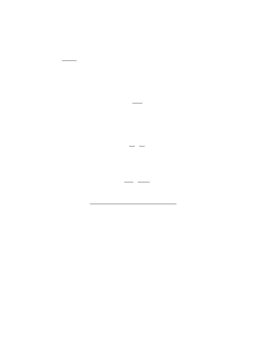
Excerpts from this work may be reproduced by instructors for distribution on a not-for-profit basis for testing or instructional purposes only to
students enrolled in courses for which the textbook has been adopted. Any other reproduction or translation of this work beyond that permitted
by Sections 107 or 108 of the 1976 United States Copyright Act without the permission of the copyright owner is unlawful.
20.8 Confirm that there are 2.2 Bohr magnetons associated with each iron atom, given that the saturation
magnetization is 1.70
× 10
6
A/m, that iron has a BCC crystal structure, and that the unit cell edge length is 0.2866
nm.
Solution
We want to confirm that there are 2.2 Bohr magnetons associated with each iron atom. Therefore, let
n
B
'
be the number of Bohr magnetons per atom, which we will calculate. This is possible using a modified and
rearranged form of Equation 20.9—that is
n
B
' =
M
s
µ
B
N
Now, N is just the number of atoms per cubic meter, which is the number of atoms per unit cell (two for BCC,
Section 3.4) divided by the unit cell volume-- that is,
N =
2
V
C
=
2
a
3
a being the BCC unit cell edge length. Thus
n
B
' =
M
s
N
µ
B
=
M
s
a
3
2
µ
B
=
(1.70
× 10
6
A / m) (0.2866
× 10
−9
m)
3
/ unit cell
[
]
(2 atoms/unit cell)(9.27
× 10
-24
A - m
2
/ BM)
= 2.16 Bohr magnetons/atom
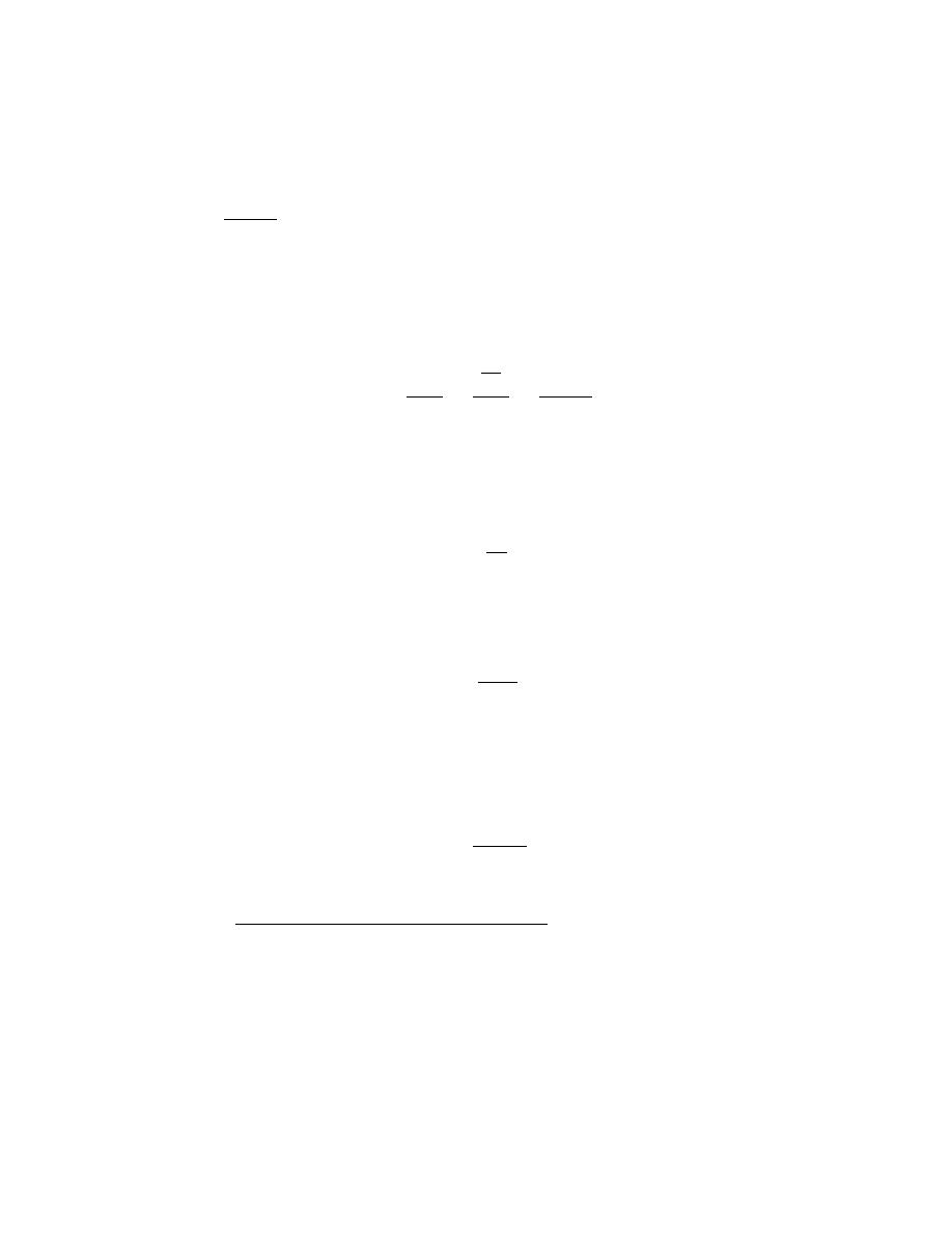
Excerpts from this work may be reproduced by instructors for distribution on a not-for-profit basis for testing or instructional purposes only to
students enrolled in courses for which the textbook has been adopted. Any other reproduction or translation of this work beyond that permitted
by Sections 107 or 108 of the 1976 United States Copyright Act without the permission of the copyright owner is unlawful.
20.9 Assume there exists some hypothetical metal that exhibits ferromagnetic behavior and that has (1) a
simple cubic crystal structure (Figure 3.24), (2) an atomic radius of 0.153 nm, and (3) a saturation flux density of
0.76 tesla. Determine the number of Bohr magnetons per atom for this material.
Solution
We are to determine the number of Bohr magnetons per atom for a hypothetical metal that has a simple
cubic crystal structure, an atomic radius of 0.153 nm, and a saturation flux density of 0.76 tesla. It becomes
necessary to employ Equation 20.8 and a modified form of Equation 20.9 as follows:
n
B =
M
s
µ
B
N
=
B
s
µ
0
µ
B
N
=
B
s
µ
0
µ
B
N
Here n
B
is the number of Bohr magnetons per atom, and N is just the number of atoms per cubic meter, which is the
number of atoms per unit cell [one for simple cubic (Figure 3.23)] divided by the unit cell volume—that is,
N =
1
V
C
which, when substituted into the above equation gives
n
B
=
B
s
V
C
µ
0
µ
B
For the simple cubic crystal structure (Figure 3.23), a = 2r, where r is the atomic radius, and V
C
= a
3
= (2r)
3
.
Substituting this relationship into the above equation yields
n
B
=
B
s (
2r
)3
µ
0
µ
B
=
(0.76 tesla)(8)
(
0.153
× 10
−9
m
)
3
(
1.257
× 10
−6
H / m
)(
9.27
× 10
−24
A - m
2
/ BM
)
= 1.87 Bohr magnetons/atom

Excerpts from this work may be reproduced by instructors for distribution on a not-for-profit basis for testing or instructional purposes only to
students enrolled in courses for which the textbook has been adopted. Any other reproduction or translation of this work beyond that permitted
by Sections 107 or 108 of the 1976 United States Copyright Act without the permission of the copyright owner is unlawful.
20.10 There is associated with each atom in paramagnetic and ferromagnetic materials a net magnetic
moment. Explain why ferromagnetic materials can be permanently magnetized whereas paramagnetic ones cannot.
Solution
Ferromagnetic materials may be permanently magnetized (whereas paramagnetic ones may not) because
of the ability of net spin magnetic moments of adjacent atoms to align with one another. This mutual magnetic
moment alignment in the same direction exists within small volume regions--domains. When a magnetic field is
applied, favorably oriented domains grow at the expense of unfavorably oriented ones, by the motion of domain
walls. When the magnetic field is removed, there remains a net magnetization by virtue of the resistance to
movement of domain walls; even after total removal of the magnetic field, the magnetization of some net domain
volume will be aligned near the direction that the external field was oriented.
For paramagnetic materials, there is no magnetic dipole coupling, and, consequently, domains do not form.
When a magnetic field is removed, the atomic dipoles assume random orientations, and no magnetic moment
remains.

Excerpts from this work may be reproduced by instructors for distribution on a not-for-profit basis for testing or instructional purposes only to
students enrolled in courses for which the textbook has been adopted. Any other reproduction or translation of this work beyond that permitted
by Sections 107 or 108 of the 1976 United States Copyright Act without the permission of the copyright owner is unlawful.
Antiferromagnetism and Ferrimagnetism
20.11 Consult another reference in which Hund’s rule is outlined, and on its basis explain the net
magnetic moments for each of the cations listed in Table 20.4.
Solution
Hund's rule states that the spins of the electrons of a shell will add together in such a way as to yield the
maximum magnetic moment. This means that as electrons fill a shell the spins of the electrons that fill the first half
of the shell are all oriented in the same direction; furthermore, the spins of the electrons that fill the last half of this
same shell will all be aligned and oriented in the opposite direction. For example, consider the iron ions in Table
20.4; from Table 2.2, the electron configuration for the outermost shell for the Fe atom is 3d
6
4s
2
. For the Fe
3+
ion
the outermost shell configuration is 3d
5
, which means that five of the ten possible 3d states are filled with electrons.
According to Hund's rule the spins of all of these electrons are aligned, there will be no cancellation, and therefore,
there are five Bohr magnetons associated with each Fe
3+
ion, as noted in the table. For Fe
2+
the configuration of
the outermost shell is 3d
6
, which means that the spins of five electrons are aligned in one direction, and the spin of a
single electron is aligned in the opposite direction, which cancels the magnetic moment of one of the other five;
thus, this yields a net moment of four Bohr magnetons.
For Mn
2+
the electron configuration is 3d
5
, the same as Fe
3+
, and, therefore it will have the same number
of Bohr magnetons (i.e., five).
For Co
2+
the electron configuration is 3d
7
, which means that the spins of five electrons are in one
direction, and two are in the opposite direction, which gives rise to a net moment of three Bohr magnetons.
For Ni
2+
the electron configuration is 3d
8
which means that the spins of five electrons are in one direction,
and three are in the opposite direction, which gives rise to a net moment of two Bohr magnetons.
For Cu
2+
the electron configuration is 3d
9
which means that the spins of five electrons are in one direction,
and four are in the opposite direction, which gives rise to a net moment of one Bohr magneton.

Excerpts from this work may be reproduced by instructors for distribution on a not-for-profit basis for testing or instructional purposes only to
students enrolled in courses for which the textbook has been adopted. Any other reproduction or translation of this work beyond that permitted
by Sections 107 or 108 of the 1976 United States Copyright Act without the permission of the copyright owner is unlawful.
20.12 Estimate (a) the saturation magnetization, and (b) the saturation flux density of nickel ferrite
[(NiFe
2
O
4
)
8
], which has a unit cell edge length of 0.8337 nm.
Solution
(a) The saturation magnetization of nickel ferrite is computed in the same manner as Example Problem
20.2; from Equation 20.13
M
s
=
n
B
µ
B
a
3
Now, n
B
is just the number of Bohr magnetons per unit cell. The net magnetic moment arises from the Ni
2+
ions,
of which there are eight per unit cell, each of which has a net magnetic moment of two Bohr magnetons (Table
20.4). Thus, n
B
is sixteen. Therefore, from the above equation
M
s
=
(16 BM / unit cell)
(
9.27
× 10
−24
A - m
2
/ BM
)
(
0.8337
× 10
−9
m
)
3
/ unit cell
= 2.56
× 10
5
A/m
(b) This portion of the problem calls for us to compute the saturation flux density. From Equation 20.8
B
s
=
µ
0
M
s
=
(
1.257
× 10
-6
H/m
)(
2.56
× 10
5
A/m
)
= 0.32 tesla
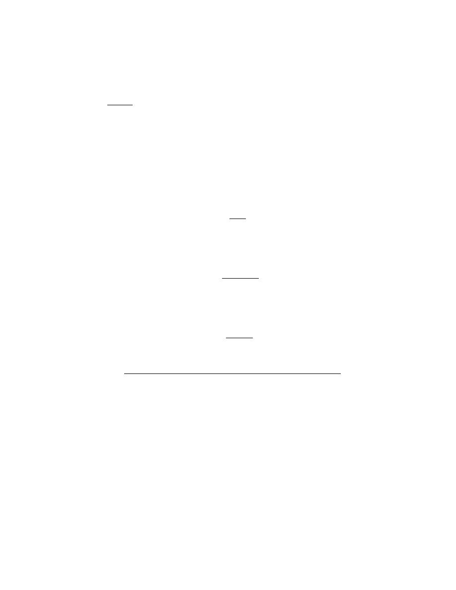
Excerpts from this work may be reproduced by instructors for distribution on a not-for-profit basis for testing or instructional purposes only to
students enrolled in courses for which the textbook has been adopted. Any other reproduction or translation of this work beyond that permitted
by Sections 107 or 108 of the 1976 United States Copyright Act without the permission of the copyright owner is unlawful.
20.13 The chemical formula for manganese ferrite may be written as (MnFe
2
O
4
)
8
because there are eight
formula units per unit cell. If this material has a saturation magnetization of 5.6
× 10
5
A/m and a density of 5.00
g/cm
3
, estimate the number of Bohr magnetons associated with each Mn
2+
ion.
Solution
We want to compute the number of Bohr magnetons per Mn
2+
ion in (MnFe
2
O
4
)
8
. Let n
B
represent the
number of Bohr magnetons per Mn
2+
ion; then, using Equation 20.9, we have
M
s
= n
B
µ
B
N
in which N is the number of Mn
2+
ions per cubic meter of material. But, from Equation 20.10
N =
ρN
A
A
Here A is the molecular weight of MnFe
2
O
4
(230.64 g/mol). Thus, combining the previous two equations
M
s
=
n
B
µ
B
ρN
A
A
or, upon rearrangement (and expressing the density in units of grams per meter cubed),
n
B
=
M
s
A
µ
B
ρN
A
=
(
5.6
× 10
5
A/m
)
(230.64 g/mol)
(
9.27
× 10
−24
A - m
2
/BM
)(
5.00
× 10
6
g/m
3
)(
6.022
× 10
23
ions / mol
)
= 4.6 Bohr magnetons/Mn
2+
ion

Excerpts from this work may be reproduced by instructors for distribution on a not-for-profit basis for testing or instructional purposes only to
students enrolled in courses for which the textbook has been adopted. Any other reproduction or translation of this work beyond that permitted
by Sections 107 or 108 of the 1976 United States Copyright Act without the permission of the copyright owner is unlawful.
20.14 The formula for yttrium iron garnet (Y
3
Fe
5
O
12
) may be written in the form
Y
3
c
Fe
2
a
Fe
3
d
O
12
, where
the superscripts a, c, and d represent different sites on which the Y
3+
and Fe
3+
ions are located. The spin magnetic
moments for the Y
3+
and Fe
3+
ions positioned in the a and c sites are oriented parallel to one another and
antiparallel to the Fe
3+
ions in d sites. Compute the number of Bohr magnetons associated with each Y
3+
ion, given
the following information: (1) each unit cell consists of eight formula (Y
3
Fe
5
O
12
) units; (2) the unit cell is cubic
with an edge length of 1.2376 nm; (3) the saturation magnetization for this material is 1.0 × 10
4
A/m; and (4)
assume that there are 5 Bohr magnetons associated with each Fe
3+
ion.
Solution
For this problem we are given that yttrium iron garnet may be written in the form
Y
3
c
Fe
2
a
Fe
3
d
O
12
where the
superscripts a, c, and d represent different sites on which the Y
3+
and Fe
3+
ions are located, and that the spin
magnetic moments for the ions on a and c sites are oriented parallel to one another and antiparallel to the Fe
3+
ions
on the d sites. We are to determine the number of Bohr magnetons associated with each Y
3+
ion given that each
unit cell consists of eight formula units, the unit cell is cubic with an edge length of 1.2376 nm, the saturation
magnetization for the material is 1.0
× 10
4
A/m, and that there are 5 Bohr magnetons for each Fe
3+
ion.
The first thing to do is to calculate the number of Bohr magnetons per unit cell, which we will denote n
B
.
Solving for n
B
using Equation 20.13, we get
n
B
=
M
s
a
3
µ
B
=
(
1.0
× 10
4
A / m
)(
1.2376
× 10
−9
m
)
3
9.27
× 10
−24
A - m
2
/ BM
= 2.04 Bohr magnetons/unit cell
Now, there are 8 formula units per unit cell or
2.04
8
= 0.255 Bohr magnetons per formula unit. Furthermore, for
each formula unit there are two Fe
3+
ions on a sites and three Fe
3+
on d sites which magnetic moments are aligned
antiparallel. Since there are 5 Bohr magnetons associated with each Fe
3+
ion, the net magnetic moment
contribution per formula unit from the Fe
3+
ions is 5 Bohr magnetons. This contribution is antiparallel to the
contribution from the Y
3+
ions, and since there are three Y
3+
ions per formula unit, then
No. of Bohr magnetons/Y
3+
=
0.255 BM
+ 5 BM
3
= 1.75 BM

Excerpts from this work may be reproduced by instructors for distribution on a not-for-profit basis for testing or instructional purposes only to
students enrolled in courses for which the textbook has been adopted. Any other reproduction or translation of this work beyond that permitted
by Sections 107 or 108 of the 1976 United States Copyright Act without the permission of the copyright owner is unlawful.
The Influence of Temperature on Magnetic Behavior
20.15 Briefly explain why the magnitude of the saturation magnetization decreases with increasing
temperature for ferromagnetic materials, and why ferromagnetic behavior ceases above the Curie temperature.
Solution
For ferromagnetic materials, the saturation magnetization decreases with increasing temperature because
the atomic thermal vibrational motions counteract the coupling forces between the adjacent atomic dipole moments,
causing some magnetic dipole misalignment. Ferromagnetic behavior ceases above the Curie temperature because
the atomic thermal vibrations are sufficiently violent so as to completely destroy the mutual spin coupling forces.

Excerpts from this work may be reproduced by instructors for distribution on a not-for-profit basis for testing or instructional purposes only to
students enrolled in courses for which the textbook has been adopted. Any other reproduction or translation of this work beyond that permitted
by Sections 107 or 108 of the 1976 United States Copyright Act without the permission of the copyright owner is unlawful.
Domains and Hysteresis
20.16 Briefly describe the phenomenon of magnetic hysteresis, and why it occurs for ferromagnetic and
ferrimagnetic materials.
The phenomenon of magnetic hysteresis and an explanation as to why it occurs for ferromagnetic and
ferrimagnetic materials is given in Section 20.7.
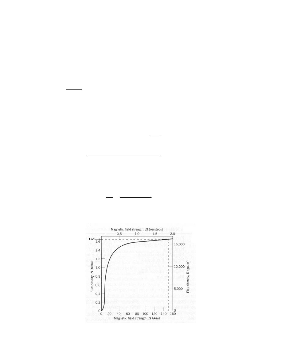
Excerpts from this work may be reproduced by instructors for distribution on a not-for-profit basis for testing or instructional purposes only to
students enrolled in courses for which the textbook has been adopted. Any other reproduction or translation of this work beyond that permitted
by Sections 107 or 108 of the 1976 United States Copyright Act without the permission of the copyright owner is unlawful.
20.17 A coil of wire 0.1 m long and having 15 turns carries a current of 1.0 A.
(a) Compute the flux density if the coil is within a vacuum.
(b) A bar of an iron–silicon alloy, the B-H behavior for which is shown in Figure 20.29, is positioned
within the coil. What is the flux density within this bar?
(c) Suppose that a bar of molybdenum is now situated within the coil. What current must be used to
produce the same B field in the Mo as was produced in the iron–silicon alloy [part (b)] using 1.0 A?
Solution
(a) This portion of the problem asks that we compute the flux density in a coil of wire 0.1 m long, having
15 turns, and carrying a current of 1.0 A, and that is situated in a vacuum. Combining Equations 20.1 and 20.3, and
solving for B yields
B
0
=
µ
0
H =
µ
0
NI
l
=
(
1.257
× 10
−6
H / m
)
(15 turns) (1.0 A)
0.1 m
= 1.89
× 10
-4
tesla
(b) Now we are to compute the flux density with a bar of the iron-silicon alloy, the B-H behavior for
which is shown in Figure 20.29. It is necessary to determine the value of H using Equation 20.1 as
H =
NI
l
=
(15 turns)(1.0 A)
0.1 m
= 150 A - turns/m
Using the curve in Figure 20.29, B = 1.65 tesla at H = 150 A-turns/m, as demonstrated below.

Excerpts from this work may be reproduced by instructors for distribution on a not-for-profit basis for testing or instructional purposes only to
students enrolled in courses for which the textbook has been adopted. Any other reproduction or translation of this work beyond that permitted
by Sections 107 or 108 of the 1976 United States Copyright Act without the permission of the copyright owner is unlawful.
(c) Finally, we are to assume that a bar of Mo is situated within the coil, and to calculate the current that is
necessary to produce the same B field as when the iron-silicon alloy in part (b) was used. Molybdenum is a
paramagnetic material having a
χ
m
of 1.19
× 10
-4
(Table 20.2). Combining Equations 20.2, 20.4, and 20.7 we solve
for H
H =
B
µ
=
B
µ
0
µ
r
=
B
µ
0
(
1
+ χ
m
)
And when Mo is positioned within the coil, then, from the above equation
H =
1.65 tesla
(
1.257
× 10
−6
H / m
)(
1
+ 1.19 x 10
−4
)
= 1.312
× 10
6
A - turns/m
Now, the current may be determined using Equation 20.1:
I =
Hl
N
=
(
1.312
× 10
6
A - turns / m
)
(0.1 m)
15 turns
= 8750 A
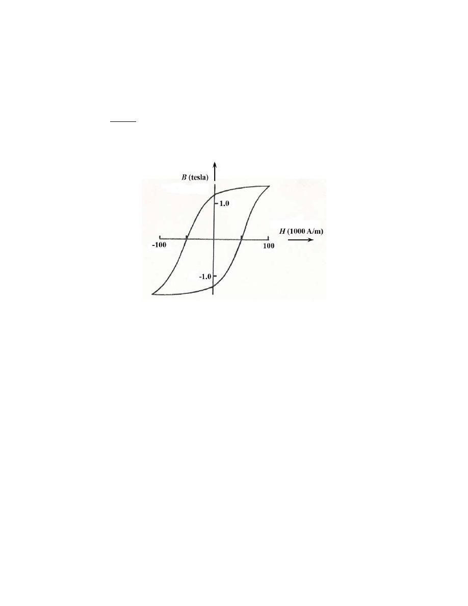
Excerpts from this work may be reproduced by instructors for distribution on a not-for-profit basis for testing or instructional purposes only to
students enrolled in courses for which the textbook has been adopted. Any other reproduction or translation of this work beyond that permitted
by Sections 107 or 108 of the 1976 United States Copyright Act without the permission of the copyright owner is unlawful.
20.18 A ferromagnetic material has a remanence of 1.25 teslas and a coercivity of 50,000 A/m. Saturation
is achieved at a magnetic field intensity of 100,000 A/m, at which the flux density is 1.50 teslas. Using these data,
sketch the entire hysteresis curve in the range H = –100,000 to +100,000 A/m. Be sure to scale and label both
coordinate axes.
Solution
The B versus H curve for this material is shown below.
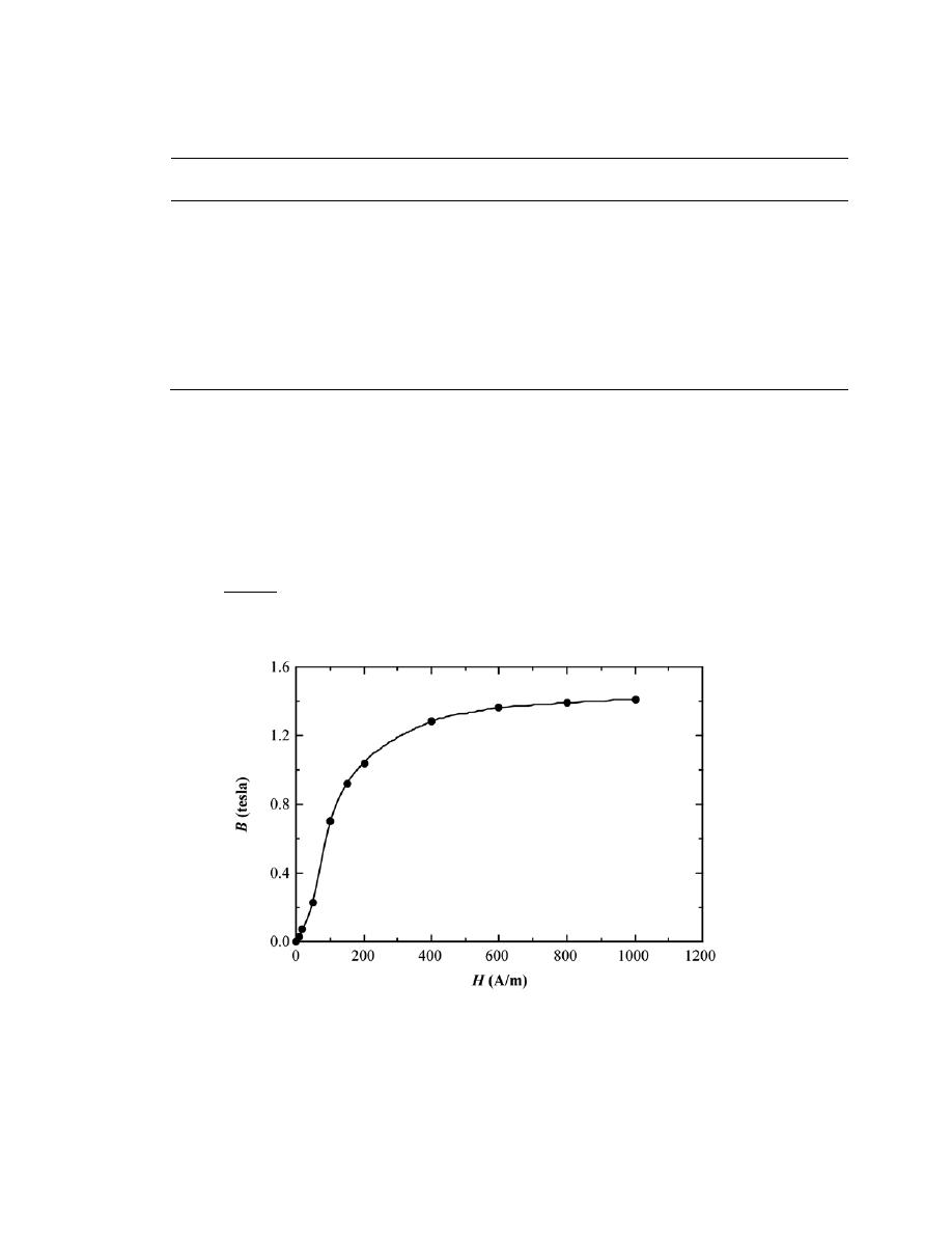
Excerpts from this work may be reproduced by instructors for distribution on a not-for-profit basis for testing or instructional purposes only to
students enrolled in courses for which the textbook has been adopted. Any other reproduction or translation of this work beyond that permitted
by Sections 107 or 108 of the 1976 United States Copyright Act without the permission of the copyright owner is unlawful.
20.19 The following data are for a transformer steel:
B
B
H (A/m)
(teslas)
H (A/m)
(teslas)
0
0
200
1.04
10
0.03
400
1.28
20
0.07
600
1.36
50
0.23
800
1.39
100
0.70
1000
1.41
150
0.92
(a) Construct a graph of B versus H.
(b) What are the values of the initial permeability and initial relative permeability?
(c) What is the value of the maximum permeability?
(d) At about what H field does this maximum permeability occur?
(e) To what magnetic susceptibility does this maximum permeability correspond?
Solution
(a) The B-H data for the transformer steel provided in the problem statement are plotted below.
(b) The first four data points are plotted below.
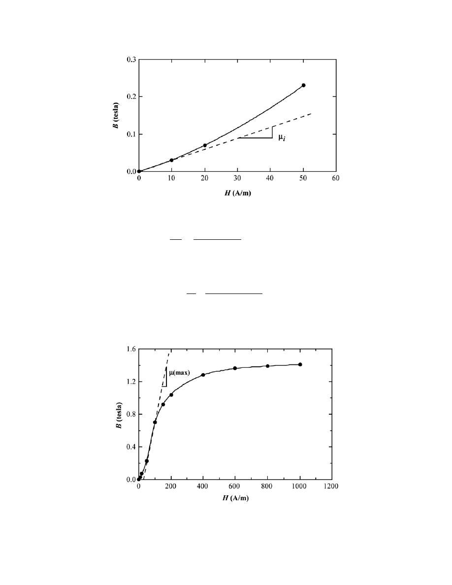
Excerpts from this work may be reproduced by instructors for distribution on a not-for-profit basis for testing or instructional purposes only to
students enrolled in courses for which the textbook has been adopted. Any other reproduction or translation of this work beyond that permitted
by Sections 107 or 108 of the 1976 United States Copyright Act without the permission of the copyright owner is unlawful.
The slope of the initial portion of the curve is
µ
i
(as shown), is
µ
i
=
∆B
∆H
=
(0.15
− 0) tesla
(50
− 0) A /m
= 3.0
× 10
-3
H/m
Also, the initial relative permeability,
µ
ri
, (Equation 20.4) is just
µ
ri
=
µ
i
µ
0
=
3.0
× 10
−3
H / m
1.257
× 10
−6
H / m
= 2387
(c) The maximum permeability is the tangent to the B-H curve having the greatest slope; it is drawn on
the plot below, and designated as
µ(max).

Excerpts from this work may be reproduced by instructors for distribution on a not-for-profit basis for testing or instructional purposes only to
students enrolled in courses for which the textbook has been adopted. Any other reproduction or translation of this work beyond that permitted
by Sections 107 or 108 of the 1976 United States Copyright Act without the permission of the copyright owner is unlawful.
The value of
µ(max) is (modifying Equation 20.2)
µ(max) =
∆B
∆H
=
(1.3
− 0.3) tesla
(160
− 45) A - m
= 8.70
× 10
-3
H/m
(d) The H field at which
µ(max) occurs is approximately 80 A/m [as taken from the plot shown in part
(c)].
(e) We are asked for the maximum susceptibility,
χ(max). Combining modified forms of Equations 20.7
and 20.4 yields
χ(max) = µ
r
(max)
− 1 =
µ (max)
µ
0
− 1
=
8.70
× 10
−3
H / m
1.257
× 10
−6
H / m
− 1 = 6920

Excerpts from this work may be reproduced by instructors for distribution on a not-for-profit basis for testing or instructional purposes only to
students enrolled in courses for which the textbook has been adopted. Any other reproduction or translation of this work beyond that permitted
by Sections 107 or 108 of the 1976 United States Copyright Act without the permission of the copyright owner is unlawful.
20.20 An iron bar magnet having a coercivity of 4000 A/m is to be demagnetized. If the bar is inserted
within a cylindrical wire coil 0.15 m long and having 100 turns, what electric current is required to generate the
necessary magnetic field?
Solution
In order to demagnetize a magnet having a coercivity of 4000 A/m, an H field of 4000 A/m must be
applied in a direction opposite to that of magnetization. According to Equation 20.1
I =
Hl
N
=
(4000 A/m) (0.15 m)
100 turns
= 6 A
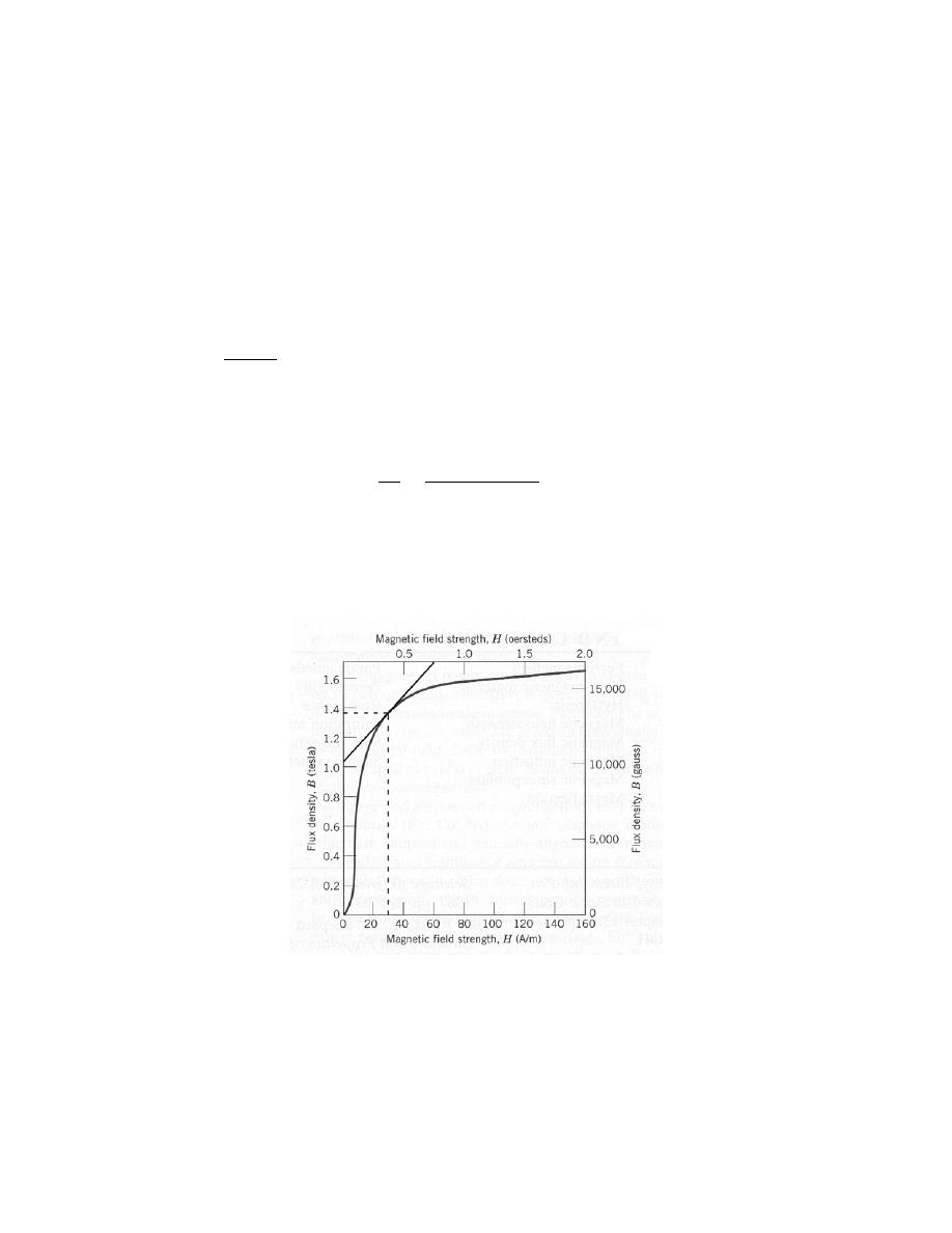
Excerpts from this work may be reproduced by instructors for distribution on a not-for-profit basis for testing or instructional purposes only to
students enrolled in courses for which the textbook has been adopted. Any other reproduction or translation of this work beyond that permitted
by Sections 107 or 108 of the 1976 United States Copyright Act without the permission of the copyright owner is unlawful.
20.21 A bar of an iron–silicon alloy having the B–H behavior shown in Figure 20.29 is inserted within a
coil of wire 0.20 m long and having 60 turns, through which passes a current of 0.1 A.
(a) What is the B field within this bar?
(b) At this magnetic field,
(i) What is the permeability?
(ii) What is the relative permeability?
(iii) What is the susceptibility?
(iv) What is the magnetization?
Solution
(a) We want to determine the magnitude of the B field within an iron-silicon alloy, the B-H behavior for
which is shown in Figure 20.29, when l = 0.20 m, N = 60 turns, and I = 0.1 A. Applying Equation 20.1
H =
NI
l
=
(60 turns) (0.1 A)
0.20 m
= 30 A/m
Below is shown the B-versus-H plot for this material. The B value from the curve corresponding to H = 30 A/m is
about 1.37 tesla.
(b)
(i) The permeability at this field is just
∆B/∆H of the tangent of the B-H curve at H = 30 A/m.
The slope of this line as drawn in the above figure is

Excerpts from this work may be reproduced by instructors for distribution on a not-for-profit basis for testing or instructional purposes only to
students enrolled in courses for which the textbook has been adopted. Any other reproduction or translation of this work beyond that permitted
by Sections 107 or 108 of the 1976 United States Copyright Act without the permission of the copyright owner is unlawful.
µ =
∆B
∆H
=
(1.70
− 1.04) tesla
(60
− 0) A /m
= 1.10
× 10
-2
H/m
(ii) From Equation 20.4, the relative permeability is
µ
r
=
µ
µ
0
=
1.10
× 10
−2
H / m
1.257
× 10
−6
H / m
= 8751
(iii) Using Equation 20.7, the susceptibility is
χ
m
=
µ
r
− 1 = 8751 − 1 = 8750
(iv) The magnetization is determined from Equation 20.6 as
M =
χ
m
H = (8750)(30 A/m) = 2.63
× 10
5
A/m

Excerpts from this work may be reproduced by instructors for distribution on a not-for-profit basis for testing or instructional purposes only to
students enrolled in courses for which the textbook has been adopted. Any other reproduction or translation of this work beyond that permitted
by Sections 107 or 108 of the 1976 United States Copyright Act without the permission of the copyright owner is unlawful.
Magnetic Anisotropy
20.22 Estimate saturation values of H for single-crystal iron in [100], [110], and [111] directions.
Solution
This problem asks for us to estimate saturation values of H for single crystal iron in the [100], [110], and
[111] directions. All we need do is read values of H at the points at which saturation is achieved on the [100],
[110], and [111] curves for iron shown in Figure 20.17. Saturation in the [100] direction is approximately 5400
A/m. Corresponding values in [110] and [111] directions are approximately 40,000 and 47,000 A/m, respectively.

Excerpts from this work may be reproduced by instructors for distribution on a not-for-profit basis for testing or instructional purposes only to
students enrolled in courses for which the textbook has been adopted. Any other reproduction or translation of this work beyond that permitted
by Sections 107 or 108 of the 1976 United States Copyright Act without the permission of the copyright owner is unlawful.
20.23 The energy (per unit volume) required to magnetize a ferromagnetic material to saturation (E
s
) is
defined by the following equation:
E
s
=
µ
0
0
M
s
∫
H dM
That is, E
s
is equal to the product of μ
0
and the area under an M versus H curve, to the point of saturation
referenced to the ordinate (or M) axis—for example, in Figure 20.17 the area between the vertical axis and the
magnetization curve to M
s
. Estimate E
s
values (in J/m
3
) for single-crystal nickel in [100], [110], and [111]
directions.
Solution
In this problem we are asked to estimate the energy required to magnetize single crystals of nickel in [100],
[110], and [111] directions. These energies correspond to the products of
µ
0
and the areas between the vertical axis
of Figure 20.17 and the three curves for single crystal nickel taken to the saturation magnetization. For the [100]
direction this area is about 15.8
× 10
8
A
2
/m
2
. When this value is multiplied by the value of
µ
0
(1.257
× 10
-6
H/m),
we get a value of about 1990 J/m
3
. The corresponding approximate areas for [110] and [111] directions are 9.6
×
10
8
A
2
/m
2
and 3.75
× 10
8
A
2
/m
2
, respectively; when multiplied by
µ
0
the respective energies for [110] and [111]
directions are 1210 and 470 J/m3.

Excerpts from this work may be reproduced by instructors for distribution on a not-for-profit basis for testing or instructional purposes only to
students enrolled in courses for which the textbook has been adopted. Any other reproduction or translation of this work beyond that permitted
by Sections 107 or 108 of the 1976 United States Copyright Act without the permission of the copyright owner is unlawful.
Soft Magnetic Materials
Hard Magnetic Materials
20.24 Cite the differences between hard and soft magnetic materials in terms of both hysteresis behavior
and typical applications.
Solution
Relative to hysteresis behavior, a hard magnetic material has a high remanence, a high coercivity, a high
saturation flux density, high hysteresis energy losses, and a low initial permeability; a soft magnetic material, on the
other hand, has a high initial permeability, a low coercivity, and low hysteresis energy losses.
With regard to applications, hard magnetic materials are utilized for permanent magnets; soft magnetic
materials are used in devices that are subjected to alternating magnetic fields such as transformer cores, generators,
motors, and magnetic amplifier devices.

Excerpts from this work may be reproduced by instructors for distribution on a not-for-profit basis for testing or instructional purposes only to
students enrolled in courses for which the textbook has been adopted. Any other reproduction or translation of this work beyond that permitted
by Sections 107 or 108 of the 1976 United States Copyright Act without the permission of the copyright owner is unlawful.
20.25 Assume that the commercial iron (99.95 wt% Fe) in Table 20.5 just reaches the point of saturation
when inserted within the coil in Problem 20.1. Compute the saturation magnetization.
Solution
We want to determine the saturation magnetization of the 99.95 wt% Fe in Table 20.5, if it just reaches
saturation when inserted within the coil described in Problem 20.1—i.e., l = 0.20 m, N = 200 turns, and A = 10 A. It
is first necessary to compute the H field within this coil using Equation 20.1 as
H
s
=
NI
l
=
(200 turns)(10 A)
0.20 m
= 10, 000 A - turns/m
Now, the saturation magnetization may be determined from a rearranged form of Equation 20.5 as
M
s
=
B
s
− µ
0
H
s
µ
0
The value of B
s
in Table 20.5 is 2.14 tesla; thus,
M
s
=
(2.14 tesla)
−
(
1.257
× 10
−6
H / m
)(
10, 000 A / m
)
1.257
× 10
−6
H / m
= 1.69
× 10
6
A/m
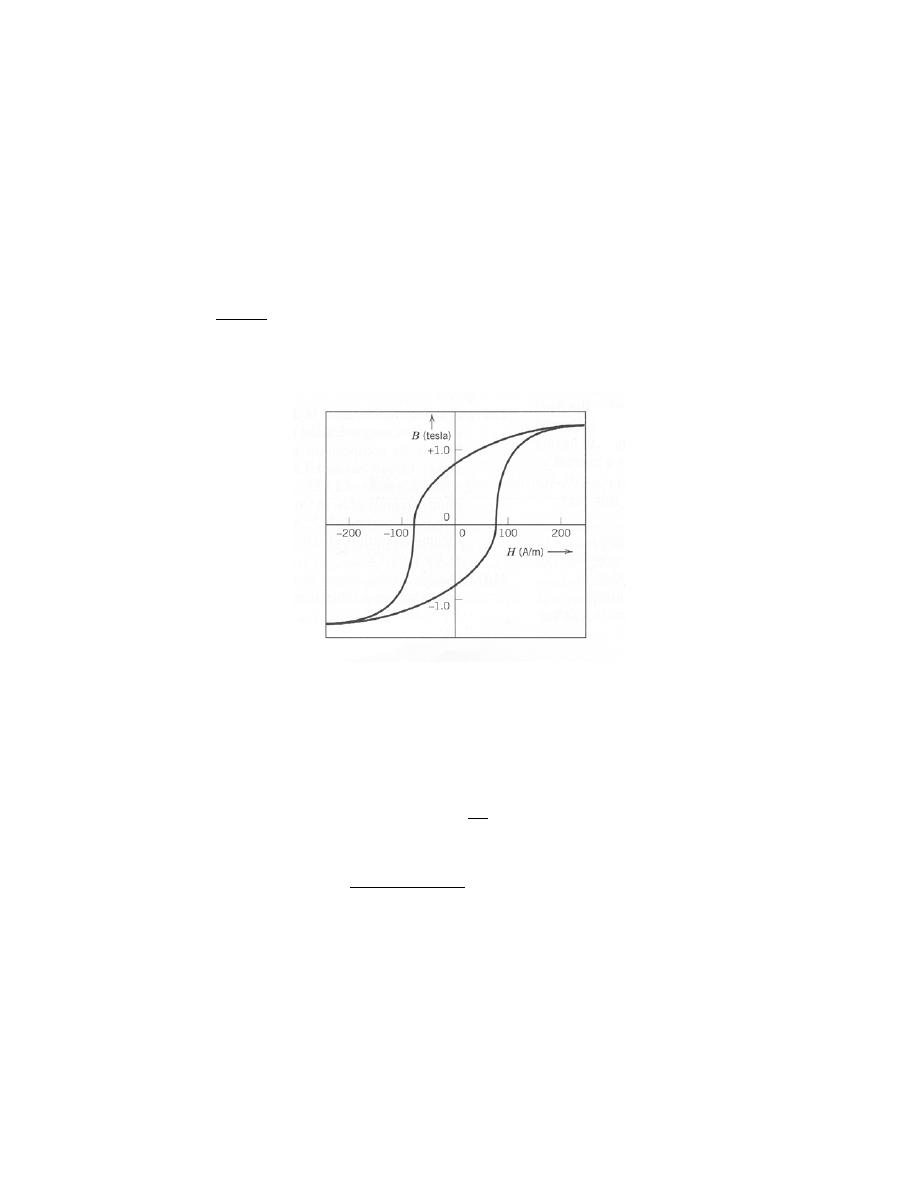
Excerpts from this work may be reproduced by instructors for distribution on a not-for-profit basis for testing or instructional purposes only to
students enrolled in courses for which the textbook has been adopted. Any other reproduction or translation of this work beyond that permitted
by Sections 107 or 108 of the 1976 United States Copyright Act without the permission of the copyright owner is unlawful.
20.26 Figure 20.30 shows the B-versus-H curve for a steel alloy.
(a) What is the saturation flux density?
(b) What is the saturation magnetization?
(c) What is the remanence?
(d) What is the coercivity?
(e) On the basis of data in Tables 20.5 and 20.6, would you classify this material as a soft or hard
magnetic material? Why?
Solution
The B-versus-H curve of Figure 20.30 is shown below.
(a) The saturation flux density for the steel, the B-H behavior for which is shown in Figure 20.30, is 1.3
tesla, the maximum B value shown on the plot.
(b) The saturation magnetization is computed from Equation 20.8 as
M
s
=
B
s
µ
0
=
1.3 tesla
1.257
× 10
−6
H / m
= 1.03
× 10
6
A/m
(c) The remanence, B
r
, is read from this plot as from the hysteresis loop shown in Figure 20.14; its value
is about 0.80 tesla.
(d) The coercivity, H
c
, is read from this plot as from Figure 20.14; the value is about 80 A/m.

Excerpts from this work may be reproduced by instructors for distribution on a not-for-profit basis for testing or instructional purposes only to
students enrolled in courses for which the textbook has been adopted. Any other reproduction or translation of this work beyond that permitted
by Sections 107 or 108 of the 1976 United States Copyright Act without the permission of the copyright owner is unlawful.
(e) On the basis of Tables 20.5 and 20.6, this is most likely a soft magnetic material. The saturation flux
density (1.3 tesla) lies within the range of values cited for soft materials, and the remanence (0.80 tesla) is close to
the values given in Table 20.6 for hard magnetic materials. However, the H
c
(80 A/m) is significantly lower than
for hard magnetic materials. Also, if we estimate the area within the hysteresis curve, we get a value of
approximately 250 J/m
3
, which is in line with the hysteresis loss per cycle for soft magnetic materials.

Excerpts from this work may be reproduced by instructors for distribution on a not-for-profit basis for testing or instructional purposes only to
students enrolled in courses for which the textbook has been adopted. Any other reproduction or translation of this work beyond that permitted
by Sections 107 or 108 of the 1976 United States Copyright Act without the permission of the copyright owner is unlawful.
Magnetic Storage
20.27 Briefly explain the manner in which information is stored magnetically.
The manner in which information is stored magnetically is discussed in Section 20.11.

Excerpts from this work may be reproduced by instructors for distribution on a not-for-profit basis for testing or instructional purposes only to
students enrolled in courses for which the textbook has been adopted. Any other reproduction or translation of this work beyond that permitted
by Sections 107 or 108 of the 1976 United States Copyright Act without the permission of the copyright owner is unlawful.
Superconductivity
20.28 For a superconducting material at a temperature T below the critical temperature T
C
, the critical
field H
C
(T), depends on temperature according to the relationship
H
C
(T) = H
C
(0) 1
−
T
2
T
C
2
(20.14)
where H
C
(0) is the critical field at 0 K.
(a) Using the data in Table 20.7, calculate the critical magnetic fields for tin at 1.5 and 2.5 K..
(b) To what temperature must tin be cooled in a magnetic field of 20,000 A/m for it to be superconductive?
Solution
(a) Given Equation 20.14 and the data in Table 20.7, we are asked to calculate the critical magnetic fields
for tin at 1.5 and 2.5 K. From the table, for Sn, T
C
= 3.72 K and B
C
(0) = 0.0305 tesla. Thus, from Equation 20.2
H
C
(0) =
B
C
(0)
µ
0
=
0.0305 tesla
1.257
× 10
−6
H / m
= 2.43
× 10
4
A/m
Now, solving for H
C
(1.5) and H
C
(2.5) using Equation 20.14 yields
H
C
(T) = H
C
(0) 1
−
T
2
T
C
2
H
C
(1.5) =
(
2.43
× 10
4
A / m
)
1
−
(1.5 K)
2
(3.72 K)
2
= 2.03 × 10
4
A/m
H
C
(2.5) =
(
2.43
× 10
4
A / m
)
1
−
(2.5 K)
2
(3.72 K)
2
= 1.33 × 10
4
A/m
(b) Now we are to determine the temperature to which tin must be cooled in a magnetic field of 20,000
A/m in order for it to be superconductive. All we need do is to solve for T from Equation 20.14—i.e.,

Excerpts from this work may be reproduced by instructors for distribution on a not-for-profit basis for testing or instructional purposes only to
students enrolled in courses for which the textbook has been adopted. Any other reproduction or translation of this work beyond that permitted
by Sections 107 or 108 of the 1976 United States Copyright Act without the permission of the copyright owner is unlawful.
T = T
C
1
−
H
C
(T)
H
C
(0)
And, since the value of H
C
(0) was computed in part (a) (i.e., 24,300 A/m), then
T = (3.72 K) 1
−
20, 000 A/m
24, 300 A/m
= 1.56 K

Excerpts from this work may be reproduced by instructors for distribution on a not-for-profit basis for testing or instructional purposes only to
students enrolled in courses for which the textbook has been adopted. Any other reproduction or translation of this work beyond that permitted
by Sections 107 or 108 of the 1976 United States Copyright Act without the permission of the copyright owner is unlawful.
20.29 Using Equation 20.14, determine which of the superconducting elements in Table 20.7 are
superconducting at 3 K and in a magnetic field of 15,000 A/m.
Solution
We are asked to determine which of the superconducting elements in Table 20.7 are superconducting at 3
K and in a magnetic field of 15,000 A/m. First of all, in order to be superconductive at 3 K within any magnetic
field, the critical temperature must be greater than 3 K. Thus, aluminum, titanium, and tungsten may be eliminated
upon inspection. Now, for each of lead, mercury, and tin it is necessary, using Equation 20.14, to compute the
value of H
C
(3)—also substituting for H
C
(0) from Equation 20.3; if H
C
(3) is greater than 15,000 A/m then the
element will be superconductive. Hence, for Pb
H
C
(2) = H
C
(0) 1
−
T
2
T
C
2
=
B
C
(0)
µ
0
1
−
T
2
T
C
2
=
0.0803 tesla
1.257
× 10
−6
H / m
1
−
(3.0 K)
2
(7.19 K)
2
= 5.28 × 10
4
A/m
Since this value is greater than 15,000 A/m, Pb will be superconductive.
Similarly for Hg
H
C
(3)
=
0.0411 tesla
1.257
× 10
−6
H / m
1
−
(3.0 K)
2
(4.15 K)
2
= 1.56 × 10
4
A/m
Inasmuch as this value is greater than 15,000 A/m, Hg will be superconductive.
As for Sn
H
C
(3)
=
0.0305 tesla
1.257
× 10
−6
H / m
1
−
(3.0 K)
2
(3.72 K)
2
= 8.48 × 10
3
A/m
Therefore, Sn is not superconductive.

Excerpts from this work may be reproduced by instructors for distribution on a not-for-profit basis for testing or instructional purposes only to
students enrolled in courses for which the textbook has been adopted. Any other reproduction or translation of this work beyond that permitted
by Sections 107 or 108 of the 1976 United States Copyright Act without the permission of the copyright owner is unlawful.
20.30 Cite the differences between type I and type II superconductors.
Solution
For type I superconductors, with increasing magnetic field the material is completely diamagnetic and
superconductive below H
C
, while at H
C
conduction becomes normal and complete magnetic flux penetration takes
place. On the other hand, for type II superconductors upon increasing the magnitude of the magnetic field, the
transition from the superconducting to normal conducting states is gradual between lower-critical and upper-critical
fields; so also is magnetic flux penetration gradual. Furthermore, type II generally have higher critical temperatures
and critical magnetic fields.

Excerpts from this work may be reproduced by instructors for distribution on a not-for-profit basis for testing or instructional purposes only to
students enrolled in courses for which the textbook has been adopted. Any other reproduction or translation of this work beyond that permitted
by Sections 107 or 108 of the 1976 United States Copyright Act without the permission of the copyright owner is unlawful.
20.31 Briefly describe the Meissner effect.
Solution
The Meissner effect is a phenomenon found in superconductors wherein, in the superconducting state, the
material is diamagnetic and completely excludes any external magnetic field from its interior. In the normal
conducting state complete magnetic flux penetration of the material occurs.

Excerpts from this work may be reproduced by instructors for distribution on a not-for-profit basis for testing or instructional purposes only to
students enrolled in courses for which the textbook has been adopted. Any other reproduction or translation of this work beyond that permitted
by Sections 107 or 108 of the 1976 United States Copyright Act without the permission of the copyright owner is unlawful.
20.32 Cite the primary limitation of the new superconducting materials that have relatively high critical
temperatures.
Solution
The primary limitation of the new superconducting materials that have relatively high critical temperatures
is that, being ceramics, they are inherently brittle.
Excerpts from this work may be reproduced by instructors for distribution on a not-for-profit basis for testing or instructional purposes only to
students enrolled in courses for which the textbook has been adopted. Any other reproduction or translation of this work beyond that permitted
by Sections 107 or 108 of the 1976 United States Copyright Act without the permission of the copyright owner is unlawful.
DESIGN PROBLEMS
Ferromagnetism
20.D1 A cobalt–nickel alloy is desired that has a saturation magnetization of 1.3 × 10
6
A/m. Specify its
composition in weight percent nickel. Cobalt has an HCP crystal structure with c/a ratio of 1.623, whereas the
maximum solubility of Ni in Co at room temperature is approximately 35 wt%. Assume that the unit cell volume for
this alloy is the same as for pure Co.
Solution
For this problem we are asked to determine the composition of a Co-Ni alloy that will yield a saturation
magnetization of 1.3
× 10
6
A/m. To begin, let us compute the number of Bohr magnetons per unit cell n
B
for this
alloy from an expression that results from combining Equations 20.11 and 20.12. That is
n
B
=
′
N V
C
=
M
s
V
C
µ
B
in which M
s
is the saturation magnetization, V
C
is the unit cell volume, and
µ
B
is the magnitude of the Bohr
magneton. According to Equation 3.S1 (the solution to Problem 3.7), for HCP
V
C
= 6 R
2
c 3
And, as stipulated in the problem statement, c = 1.623a; in addition, for HCP, the unit cell edge length, a, and the
atomic radius, R are related as a = 2R. Making these substitutions into the above equation leads to the following:
V
C
= 6 R
2
c 3
= 6 R
2
(1.623a) 3
= 6 R
2
(1.623)(2R) 3
= 12 R
3
(1.623) 3
From the inside of the front cover of the book, the value of R for Co is given as 0.125 nm (1.25
× 10
-10
m).
Therefore,
V
C
= (12)
(
1.25
× 10
-10
m
)
3
(1.623) 3
= 6.59
× 10
-29
m
3

Excerpts from this work may be reproduced by instructors for distribution on a not-for-profit basis for testing or instructional purposes only to
students enrolled in courses for which the textbook has been adopted. Any other reproduction or translation of this work beyond that permitted
by Sections 107 or 108 of the 1976 United States Copyright Act without the permission of the copyright owner is unlawful.
And, now solving for n
B
from the first equation above, yields
n
B
= =
M
s
V
C
µ
B
=
(
1.3
× 10
6
A / m
)(
6.59
× 10
−29
m
3
/ unit cell
)
9.27
× 10
−24
A - m
2
Bohr magneton
= 9.24
Bohr magneton
unit cell
Inasmuch as there are 1.72 and 0.60 Bohr magnetons for each of Co and Ni (Section 20.4), and, for HCP, there are
6 equivalent atoms per unit cell (Section 3.4), if we represent the fraction of Ni atoms by x, then
n
B
= 9.24 Bohr magnetons/unit cell
=
0.60 Bohr magnetons
Ni atom
6 x Ni atoms
unit cell
+
1.72 Bohr magnetons
Co atom
(6) (1
− x) Co atoms
unit cell
And solving for x, the fraction of Ni atoms , x = 0.161, or 16.1 at% Ni.
In order to convert this composition to weight percent, we employ Equation 4.7 as
C
Ni
=
C
Ni
' A
Ni
C
Ni
' A
Ni
+ C
Co
' A
Co
× 100
=
(16.1 at%)(58.69 g/mol)
(16.1 at%)(58.69 g/mol)
+ (83.9 at%)(58.93 g/mol)
× 100
= 16.0 wt%

Excerpts from this work may be reproduced by instructors for distribution on a not-for-profit basis for testing or instructional purposes only to
students enrolled in courses for which the textbook has been adopted. Any other reproduction or translation of this work beyond that permitted
by Sections 107 or 108 of the 1976 United States Copyright Act without the permission of the copyright owner is unlawful.
Ferrimagnetism
20.D2 Design a cubic mixed-ferrite magnetic material that has a saturation magnetization of 4.6
× 10
5
A/m.
Solution
This problem asks that we design a cubic mixed-ferrite magnetic material that has a saturation
magnetization of 4.6
× 10
5
A/m. From Example Problem 20.2 the saturation magnetization for Fe
3
O
4
is 5.0
× 10
5
A/m. In order to decrease the magnitude of M
s
it is necessary to replace some fraction of the Fe
2+
with another
divalent metal ion that has a smaller magnetic moment. From Table 20.4 it may be noted that Co
2+
, Ni
2+
, and
Cu
2+
, with 3, 2, and 1 Bohr magnetons per ion, respectively, have fewer than the 4 Bohr magnetons/Fe
2+
ion. Let
us first consider Co
2+
(with 3 Bohr magnetons per ion) and employ Equation 20.13 to compute the number of Bohr
magnetons per unit cell (n
B
), assuming that the Co
2+
addition does not change the unit cell edge length (0.839 nm,
Example Problem 20.2). Thus,
n
B
=
M
s
a
3
µ
B
=
(
4.6
× 10
5
A/m
)(
0.839
× 10
−9
m
)
3
/unit cell
9.27
× 10
−24
A - m
2
/Bohr magneton
= 29.31 Bohr magnetons/unit cell
If we let x
Co
represent the fraction of Co
2+
that have substituted for Fe
2+
, then the remaining unsubstituted Fe
2+
fraction is equal to 1 – x
Co
. Furthermore, inasmuch as there are 8 divalent ions per unit cell, we may write the
following expression:
n
B
(Co) = 8 3x
Co
+ 4(1
− x
Co
)
[
]
= 29.31
which leads to x
Co
= 0.336. Thus, if 33.6 at% of the Fe
2+
in Fe
3
O
4
are replaced with Co
2+
, the saturation
magnetization will be decreased to 4.6
× 10
5
A/m.
For the cases of Ni
2+
and Cu
2+
substituting for Fe
2+
, the equivalents of the preceding equation for the
number of Bohr magnetons per unit cell will read as follows:

Excerpts from this work may be reproduced by instructors for distribution on a not-for-profit basis for testing or instructional purposes only to
students enrolled in courses for which the textbook has been adopted. Any other reproduction or translation of this work beyond that permitted
by Sections 107 or 108 of the 1976 United States Copyright Act without the permission of the copyright owner is unlawful.
n
B
(Ni) = 8 2x
Ni
+ 4(1
− x
Ni
)
[
]
= 29.31
n
B
(Cu) = 8 x
Cu
+ 4(1
− x
Cu
)
[
]
= 29.31
with the results that
x
Ni
= 0.168 (or 16.8 at%)
x
Cu
= 0.112 (11.2 at%)
will yield the 4.6
× 10
5
A/m saturation magnetization.

Excerpts from this work may be reproduced by instructors for distribution on a not-for-profit basis for testing or instructional purposes only to
students enrolled in courses for which the textbook has been adopted. Any other reproduction or translation of this work beyond that permitted
by Sections 107 or 108 of the 1976 United States Copyright Act without the permission of the copyright owner is unlawful.
CHAPTER 21
OPTICAL PROPERTIES
Electromagnetic Radiation
21.1 Visible light having a wavelength of 6
× 10
-7
m appears orange. Compute the frequency and energy
of a photon of this light.
Solution
In order to compute the frequency of a photon of orange light, we must use Equation 21.2 as
ν =
c
λ
=
3
× 10
8
m /s
6
× 10
−7
m
= 5
× 10
14
s
-1
Now, for the energy computation, we employ Equation 21.3 as follows:
E =
hc
λ
=
(
6.63
× 10
−34
J - s
)(
3
× 10
8
m /s
)
6
× 10
−7
m
= 3.31
× 10
-19
J (2.07 eV)

Excerpts from this work may be reproduced by instructors for distribution on a not-for-profit basis for testing or instructional purposes only to
students enrolled in courses for which the textbook has been adopted. Any other reproduction or translation of this work beyond that permitted
by Sections 107 or 108 of the 1976 United States Copyright Act without the permission of the copyright owner is unlawful.
Light Interactions with Solids
21.2 Distinguish between materials that are opaque, translucent, and transparent in terms of their
appearance and light transmittance.
Solution
Opaque materials are impervious to light transmission; it is not possible to see through them.
Light is transmitted diffusely through translucent materials (there is some internal light scattering). Objects
are not clearly distinguishable when viewed through a translucent material.
Virtually all of the incident light is transmitted through transparent materials, and one can see clearly
through them.

Excerpts from this work may be reproduced by instructors for distribution on a not-for-profit basis for testing or instructional purposes only to
students enrolled in courses for which the textbook has been adopted. Any other reproduction or translation of this work beyond that permitted
by Sections 107 or 108 of the 1976 United States Copyright Act without the permission of the copyright owner is unlawful.
Atomic and Electronic Interactions
21.3 (a) Briefly describe the phenomenon of electronic polarization by electromagnetic radiation. (b)
What are two consequences of electronic polarization in transparent materials?
Solution
(a) The phenomenon of electronic polarization by electromagnetic radiation is described in Section 21.4.
(b) Two consequences of electronic polarization in transparent materials are absorption and refraction.

Excerpts from this work may be reproduced by instructors for distribution on a not-for-profit basis for testing or instructional purposes only to
students enrolled in courses for which the textbook has been adopted. Any other reproduction or translation of this work beyond that permitted
by Sections 107 or 108 of the 1976 United States Copyright Act without the permission of the copyright owner is unlawful.
Optical Properties of Metals
21.4 Briefly explain why metals are opaque to electromagnetic radiation having photon energies within
the visible region of the spectrum.
Solution
The electron band structures of metals are such that empty and available electron states are adjacent to
filled states. Electron excitations from filled to empty states are possible with the absorption of electromagnetic
radiation having frequencies within the visible spectrum, according to Equation 21.6. The light energy is totally
absorbed or reflected, and, since none is transmitted, the material is opaque.

Excerpts from this work may be reproduced by instructors for distribution on a not-for-profit basis for testing or instructional purposes only to
students enrolled in courses for which the textbook has been adopted. Any other reproduction or translation of this work beyond that permitted
by Sections 107 or 108 of the 1976 United States Copyright Act without the permission of the copyright owner is unlawful.
Refraction
21.5 In ionic materials, how does the size of the component ions affect the extent of electronic
polarization?
Solution
In ionic materials, the larger the size of the component ions the greater the degree of electronic
polarization.

Excerpts from this work may be reproduced by instructors for distribution on a not-for-profit basis for testing or instructional purposes only to
students enrolled in courses for which the textbook has been adopted. Any other reproduction or translation of this work beyond that permitted
by Sections 107 or 108 of the 1976 United States Copyright Act without the permission of the copyright owner is unlawful.
21.6 Can a material have an index of refraction less than unity? Why or why not?
Solution
In order for a material to have an index of refraction less than unity, the velocity of light in the material (v)
would necessarily have to be greater than the velocity of light in a vacuum (Equation 21.7). This is not possible.
Excerpts from this work may be reproduced by instructors for distribution on a not-for-profit basis for testing or instructional purposes only to
students enrolled in courses for which the textbook has been adopted. Any other reproduction or translation of this work beyond that permitted
by Sections 107 or 108 of the 1976 United States Copyright Act without the permission of the copyright owner is unlawful.
21.7 Compute the velocity of light in calcium fluoride (CaF
2
), which has a dielectric constant
∈
r
of 2.056
(at frequencies within the visible range) and a magnetic susceptibility of -1.43
× 10
-5
.
Solution
We want to compute the velocity of light in calcium fluoride given that
ε
r
= 2.056 and
χ
m
= -1.43
× 10
-5
.
The velocity is determined using Equation 21.8; but first, we must calculate the values of
ε and µ for calcium
fluoride. According to Equation 18.27
ε = ε
r
ε
0
= (2.056)
(
8.85
× 10
-12
F/m
)
= 1.82
× 10
-11
F/m
Now, combining Equations 20.4 and 20.7
µ = µ
0
µ
r
= µ
0
(
χ
m
+ 1
)
=
(
1.257
× 10
-6
H/m
)(
1
− 1.43 × 10
-5
)
= 1.257
× 10
-6
H/m
And, finally, from Equation 21.8
v =
1
εµ
=
1
(
1.82
× 10
−11
F / m
)(
1.257
× 10
−6
H / m
)
= 2.09
× 10
8
m/s

Excerpts from this work may be reproduced by instructors for distribution on a not-for-profit basis for testing or instructional purposes only to
students enrolled in courses for which the textbook has been adopted. Any other reproduction or translation of this work beyond that permitted
by Sections 107 or 108 of the 1976 United States Copyright Act without the permission of the copyright owner is unlawful.
21.8 The indices of refraction of fused silica and a soda–lime glass within the visible spectrum are 1.458
and 1.51, respectively. For each of these materials determine the fraction of the relative dielectric constant at 60 Hz
that is due to electronic polarization, using the data of Table 18.5. Neglect any orientation polarization effects.
Solution
The frequencies of visible radiation are on the order of 10
15
Hz (Figure 21.2). At these frequencies only
electronic polarization is operable (Figure 18.34). Thus,
ε
r
from Equation 21.10 is the electronic contribution to
ε
r
;
let us designate it as
ε
r
' . Or, in other words
ε
r
'
= n
2
For fused silica
ε
r
'
(silica) = (1.458)
2
= 2.13
And, for soda-lime glass
ε
r
'
(glass) = (1.51)
2
= 2.28
The fraction of the electronic contribution is just the ratio of
ε
r
'
and
ε
r
, where
ε
r
values are taken from Table 18.5
(4.0 and 6.9 for fused silica and soda-lime glass, respectively). Thus
ε
r
'
(silica)
ε
r
(60 Hz)
=
2.13
4.0
= 0.53
and
ε
r
'
(glass)
ε
r
(60 Hz)
=
2.28
6.9
= 0.33
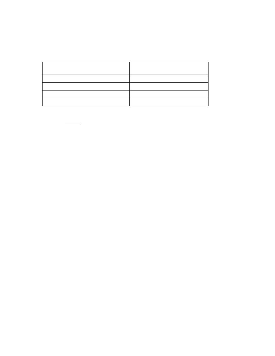
Excerpts from this work may be reproduced by instructors for distribution on a not-for-profit basis for testing or instructional purposes only to
students enrolled in courses for which the textbook has been adopted. Any other reproduction or translation of this work beyond that permitted
by Sections 107 or 108 of the 1976 United States Copyright Act without the permission of the copyright owner is unlawful.
21.9 Using the data in Table 21.1, estimate the dielectric constants for borosilicate glass, periclase
(MgO), poly(methyl methacrylate), and polypropylene, and compare these values with those cited in the table
below. Briefly explain any discrepancies.
Material
Dielectric Constant
(1 MHz)
Borosilicate glass
4.65
Periclase
9.65
Poly(methyl methacrylate)
2.76
Polypropylene
2.30
Solution
This problem asks for us, using data in Table 21.1, to estimate the dielectric constants for borosilicate
glass, periclase (MgO), poly(methyl methacrylate), and polypropylene, and then to compare these values with those
cited in the table provided, and briefly explain any discrepancies. From Equation 21.10
ε
r
= n
2
Thus, for borosilicate glass, since n = 1.47
ε
r
= (1.47)
2
= 2.16
Similarly, for periclase
ε
r
= (1.74)
2
= 3.03
And, for PMMA
ε
r
= (1.49)
2
= 2.22
For polypropylene
ε
r
= (1.49)
2
= 2.22

Excerpts from this work may be reproduced by instructors for distribution on a not-for-profit basis for testing or instructional purposes only to
students enrolled in courses for which the textbook has been adopted. Any other reproduction or translation of this work beyond that permitted
by Sections 107 or 108 of the 1976 United States Copyright Act without the permission of the copyright owner is unlawful.
When we compare the values of
ε
r
for the polymers with those in the table at frequencies of 1 MHz, there is
reasonable agreement (i.e., 2.22 versus 2.76 for PMMA, and 2.22 versus 2.30 for polypropylene). However, for
borosilicate glass and periclase there are some significant discrepancies (i.e., 2.16 versus 4.65 for the borosilicate
glass, and 3.03 versus 9.65 for the periclase). The reason for these discrepancies is that for these two materials an
ionic component to the dielectric constant is present at 1 MHz, but is absent at frequencies within the visible
electromagnetic spectrum, which frequencies are on the order 10
9
MHz (10
15
Hz). These effects may be noted in
Figure 18.34.

Excerpts from this work may be reproduced by instructors for distribution on a not-for-profit basis for testing or instructional purposes only to
students enrolled in courses for which the textbook has been adopted. Any other reproduction or translation of this work beyond that permitted
by Sections 107 or 108 of the 1976 United States Copyright Act without the permission of the copyright owner is unlawful.
21.10 Briefly describe the phenomenon of dispersion in a transparent medium.
Solution
Dispersion in a transparent medium is the phenomenon wherein the index of refraction varies slightly with
the wavelength of the electromagnetic radiation.
Excerpts from this work may be reproduced by instructors for distribution on a not-for-profit basis for testing or instructional purposes only to
students enrolled in courses for which the textbook has been adopted. Any other reproduction or translation of this work beyond that permitted
by Sections 107 or 108 of the 1976 United States Copyright Act without the permission of the copyright owner is unlawful.
Reflection
21.11 It is desired that the reflectivity of light at normal incidence to the surface of a transparent medium
be less than 6.0%. Which of the following materials in Table 21.1 are likely candidates: silica glass, Pyrex glass,
corundum, spinel, polystyrene, and polytetrafluoroethylene? Justify your selection(s).
Solution
For this problem we want to compute the maximum value of n
s
in Equation 21.13 that will give R = 0.060.
Then we are to consult Table 21.1 in order to ascertain which of the materials listed have indices of refraction less
than this maximum value. From Equation 21.13
0.060 =
(
ns − 1
)
2
(
ns +1
)
2
=
n
s
2
− 2 n
s
+ 1
n
s
2
+ 2 n
s
+ 1
or, upon rearrangement
0.94 n
s
2
− 2.12 n
s
+ 0.94 = 0
The value of n
s
is determined by using the quadratic equation solution as follows:
n
s
=
− (−2.12) ± (− 2.12)
2
− (4)(0.94)(0.94)
(2)(0.94)
=
2.12
± 0.98
1.88
The two solutions are: n
s
(+) = 1.65 and n
s
(–) = 0.606. The n
s
(+) solution is the one that is physically reasonable.
Thus, of the materials listed, silica glass, Pyrex glass, polystyrene, and PTFE have indices of refraction less than
1.65, and would be suitable for this application.

Excerpts from this work may be reproduced by instructors for distribution on a not-for-profit basis for testing or instructional purposes only to
students enrolled in courses for which the textbook has been adopted. Any other reproduction or translation of this work beyond that permitted
by Sections 107 or 108 of the 1976 United States Copyright Act without the permission of the copyright owner is unlawful.
21.12 Briefly explain how reflection losses of transparent materials are minimized by thin surface
coatings.
Solution
The thickness and dielectric constant of a thin surface coating are selected such that there is destructive
interference between the light beam that is reflected from the lens-coating interface and the light beam that is
reflected from the coating-air interface; thus, the net intensity of the total reflected beam is very low.

Excerpts from this work may be reproduced by instructors for distribution on a not-for-profit basis for testing or instructional purposes only to
students enrolled in courses for which the textbook has been adopted. Any other reproduction or translation of this work beyond that permitted
by Sections 107 or 108 of the 1976 United States Copyright Act without the permission of the copyright owner is unlawful.
21.13 The index of refraction of corundum (Al
2
O
3
) is anisotropic. Suppose that visible light is passing
from one grain to another of different crystallographic orientation and at normal incidence to the grain boundary.
Calculate the reflectivity at the boundary if the indices of refraction for the two grains are 1.757 and 1.779 in the
direction of light propagation.
Solution
This problem calls for a calculation of the reflectivity between two corundum grains having different
orientations and indices of refraction (1.757 and 1.779) in the direction of light propagation, when the light is at
normal incidence to the grain boundary. We must employ Equation 21.12 since the beam is normal to the grain
boundary. Thus,
R =
n
2
− n
1
n
2
+ n
1
2
=
1.779
− 1.757
1.779
+ 1.757
2
= 3.87
× 10
-5

Excerpts from this work may be reproduced by instructors for distribution on a not-for-profit basis for testing or instructional purposes only to
students enrolled in courses for which the textbook has been adopted. Any other reproduction or translation of this work beyond that permitted
by Sections 107 or 108 of the 1976 United States Copyright Act without the permission of the copyright owner is unlawful.
Absorption
21.14 Zinc telluride has a band gap of 2.26 eV. Over what range of wavelengths of visible light is it
transparent?
Solution
This problem asks us to determine the range of visible light wavelengths over which ZnTe (E
g
= 2.26 eV)
is transparent. Only photons having energies of 2.26 eV or greater are absorbed by valence-band-to-conduction-
band electron transitions. Thus, photons having energies less than 2.26 eV are not absorbed; the minimum photon
energy for visible light is 1.8 eV (Equation 21.16b), which corresponds to a wavelength of 0.7
µm. From Equation
21.3, the wavelength of a photon having an energy of 2.26 eV (i.e., the band-gap energy) is just
λ =
hc
E
=
(
4.13
× 10
−15
eV - s
)(
3
× 10
8
m /s
)
2.26 eV
= 5.5
× 10
-7
m = 0.55
µm
Thus, pure ZnTe is transparent to visible light having wavelengths between 0.55 and 0.7
µm.

Excerpts from this work may be reproduced by instructors for distribution on a not-for-profit basis for testing or instructional purposes only to
students enrolled in courses for which the textbook has been adopted. Any other reproduction or translation of this work beyond that permitted
by Sections 107 or 108 of the 1976 United States Copyright Act without the permission of the copyright owner is unlawful.
21.15
Briefly explain why the magnitude of the absorption coefficient (β in Equation 21.18) depends on
the radiation wavelength.
Solution
The magnitude of the absorption coefficient (
β in Equation 21.18) depends on the radiation wavelength for
intrinsic insulators and semiconducting materials. This is because, for photons having energies less than the band-
gap energy (or in terms of wavelength, when
λ >
h c
E
g
), photon absorption due to valence-band-to-conduction-band
electron transitions are not possible, and, therefore, the value of
β will be relatively small. On the other hand, when
photons having energies equal to or greater than the band gap energy (i.e., when
λ ≤
h c
E
g
) these electron transitions
by the absorption of photons will occur with the result that the magnitude of
β will be relatively large.
In addition, there may be impurity levels that lie within the band gap (Section 21.7) from or to which
electron excitations may occur with the absorption of light radiation at specific wavelengths.

Excerpts from this work may be reproduced by instructors for distribution on a not-for-profit basis for testing or instructional purposes only to
students enrolled in courses for which the textbook has been adopted. Any other reproduction or translation of this work beyond that permitted
by Sections 107 or 108 of the 1976 United States Copyright Act without the permission of the copyright owner is unlawful.
21.16 The fraction of nonreflected radiation that is transmitted through a 10-mm thickness of a
transparent material is 0.90. If the thickness is increased to 20 mm, what fraction of light will be transmitted?
Solution
In this problem we are asked to calculate the fraction of nonreflected light transmitted through a 20-mm
thickness of transparent material, given that the fraction transmitted through a 10-mm thickness is 0.90. From
Equation 21.18, the fraction of nonreflected light transmitted is just
I
T
' / I
0
' . Using this expression we must first
determine the value of
β; this is possible by algebraic manipulation of Equation 21.18. Dividing both sides of the
equation by
I
0
' , and then taking natural logarithms leads to
ln
I
T
'
I
0
'
= −βx
Now solving for
β and also incorporating values for
I
T
' / I
0
' and x provided in the problem statement gives
β = −
1
x
ln
I
T
'
I
0
'
=
−
1
10 mm
ln (0.90) = 1.05 × 10
-2
mm
-1
And computation of
I
T
' / I
0
' when x = 20 mm (Equation 21.18) is as follows:
I
T
'
I
0
'
= exp (
− βx)
= exp
−
(
1.05
× 10
−2
mm
−1
)
(20 mm)
[
]
= 0.81

Excerpts from this work may be reproduced by instructors for distribution on a not-for-profit basis for testing or instructional purposes only to
students enrolled in courses for which the textbook has been adopted. Any other reproduction or translation of this work beyond that permitted
by Sections 107 or 108 of the 1976 United States Copyright Act without the permission of the copyright owner is unlawful.
Transmission
21.17 Derive Equation 21.19, starting from other expressions given in the chapter.
Solution
The problem asks that we derive Equation 21.19, which is
I
T
= I
0
(1
− R)
2
e−
βl
If we examine Figure 21.7, at the front (or left) interface, some of the incident beam having intensity I
0
is reflected.
Since I
R
= I
0
R at this surface, then
I
T
' = I
0
− I
0
R = I
0
(1
− R)
in which
I
T
'
is the intensity of the nonreflected beam at the front surface that is transmitted.
Now there will be absorption of this transmitted beam as it passes through the solid and transparent
medium according to Equation 21.18. Just inside the back (or right) interface, the beam has passed through a
thickness l of this material (x = l) and, therefore, the intensity of the transmitted beam at this point
(I
T
'' ) is just
I
T
'' = I
0
(1
− R)e-
βl
Finally, a second reflection will occur at the back interface as the beam passes out of the medium. The
intensity of the reflected beam
(I
R
'' )
is just
I
R
'' = I
T
'' R
= I
0
R(1
− R)e-
βl
And the intensity of the final transmitted beam (I
T
) becomes
I
T
= I
T
''
− I
R
''
= I
0
(1
− R)e-
βl
− I
0
R(1
− R)e-
βl
= I
0
(1
− R)
2
e-
βl
which is Equation 21.19, the desired expression.

Excerpts from this work may be reproduced by instructors for distribution on a not-for-profit basis for testing or instructional purposes only to
students enrolled in courses for which the textbook has been adopted. Any other reproduction or translation of this work beyond that permitted
by Sections 107 or 108 of the 1976 United States Copyright Act without the permission of the copyright owner is unlawful.
21.18 The transmissivity T of a transparent material 20 mm thick to normally incident light is 0.85. If the
index of refraction of this material is 1.6, compute the thickness of material that will yield a transmissivity of 0.75.
All reflection losses should be considered.
Solution
We are asked to compute the thickness of material to yield a transmissivity of 0.75 given that T is 0.85
when l = 20 mm, n = 1.6, and for normally incident radiation. The first requirement is that we calculate the value of
β for this material using Equations 21.13 and 21.19. The value of R is determined using Equation 21.13 as
R =
(
n
s
− 1
)
2
(
n
s
+1
)
2
=
(1.6
− 1)
2
(1.6
+ 1)
2
= 5.33
× 10
-2
Now, it is necessary to compute the value of
β using Equation 21.19. Dividing both sides of Equation 21.19 by I
0
(1
– R)
2
leads to
I
T
I
0
(1
− R)
2
= e
-
βl
And taking the natural logarithms of both sides of this expression gives
ln
I
T
I
0
(1
− R)
2
= −βl
and solving for
β we get
β = −
1
l
ln
I
T
I
0
(1
− R)
2
Since the transmissivity is T is equal to I
T
/I
0
, then the above equation takes the form
β = −
1
l
ln
T
(1
− R)
2

Excerpts from this work may be reproduced by instructors for distribution on a not-for-profit basis for testing or instructional purposes only to
students enrolled in courses for which the textbook has been adopted. Any other reproduction or translation of this work beyond that permitted
by Sections 107 or 108 of the 1976 United States Copyright Act without the permission of the copyright owner is unlawful.
Using values for l and T provided in the problem statement, as well as the value of R determined above, we solve
for
β as
β = −
1
20 mm
ln
0.85
(
1
− 5.33 × 10
−2
)
2
= 2.65 × 10
-3
mm
-1
Now, solving for l when T = 0.75 using the rearranged form of Equation 21.19 above
l =
−
1
β
ln
T
(1
− R)
2
=
−
1
2.65
× 10
−3
mm
−1
ln
0.75
(
1
− 5.33 × 10
−2
)
2
= 67.3 mm

Excerpts from this work may be reproduced by instructors for distribution on a not-for-profit basis for testing or instructional purposes only to
students enrolled in courses for which the textbook has been adopted. Any other reproduction or translation of this work beyond that permitted
by Sections 107 or 108 of the 1976 United States Copyright Act without the permission of the copyright owner is unlawful.
Color
21.19 Briefly explain what determines the characteristic color of (a) a metal and (b) a transparent
nonmetal.
Solution
(a) The characteristic color of a metal is determined by the distribution of wavelengths of the nonabsorbed
light radiation that is reflected.
(b) The characteristic color of a transparent nonmetal is determined by the distribution of wavelengths of
the nonabsorbed light radiation that is transmitted through the material.

Excerpts from this work may be reproduced by instructors for distribution on a not-for-profit basis for testing or instructional purposes only to
students enrolled in courses for which the textbook has been adopted. Any other reproduction or translation of this work beyond that permitted
by Sections 107 or 108 of the 1976 United States Copyright Act without the permission of the copyright owner is unlawful.
21.20 Briefly explain why some transparent materials appear colored while others are colorless.
Solution
For a transparent material that appears colorless, any absorption within its interior is the same for all visible
wavelengths. On the other hand, if there is any selective absorption of visible light (usually by electron excitations),
the material will appear colored, its color being dependent on the frequency distribution of the transmitted light
beam.

Excerpts from this work may be reproduced by instructors for distribution on a not-for-profit basis for testing or instructional purposes only to
students enrolled in courses for which the textbook has been adopted. Any other reproduction or translation of this work beyond that permitted
by Sections 107 or 108 of the 1976 United States Copyright Act without the permission of the copyright owner is unlawful.
Opacity and Translucency in Insulators
21.21 Briefly describe the three absorption mechanisms in nonmetallic materials.
The three absorption mechanisms in nonmetallic materials involve electronic polarization, electron
transitions, and scattering. Electronic polarization is described in Section 21.4; absorption by electron transitions is
discussed in Sections 21.4 and 21.7; and scattering is discussed in Section 21.10.

Excerpts from this work may be reproduced by instructors for distribution on a not-for-profit basis for testing or instructional purposes only to
students enrolled in courses for which the textbook has been adopted. Any other reproduction or translation of this work beyond that permitted
by Sections 107 or 108 of the 1976 United States Copyright Act without the permission of the copyright owner is unlawful.
21.22 Briefly explain why amorphous polymers are transparent, while predominantly crystalline polymers
appear opaque or, at best, translucent.
Solution
Amorphous polymers are normally transparent because there is no scattering of a light beam within the
material. However, for semicrystalline polymers, visible light will be scattered at boundaries between amorphous
and crystalline regions since they have different indices of refraction. This leads to translucency or, for extensive
scattering, opacity, except for semicrystalline polymers having very small crystallites.

Excerpts from this work may be reproduced by instructors for distribution on a not-for-profit basis for testing or instructional purposes only to
students enrolled in courses for which the textbook has been adopted. Any other reproduction or translation of this work beyond that permitted
by Sections 107 or 108 of the 1976 United States Copyright Act without the permission of the copyright owner is unlawful.
Luminescence
Photoconductivity
Lasers
21.23 (a) In your own words describe briefly the phenomenon of luminescence.
(b) What is the distinction between fluorescence and phosphorescence?
Solution
(a) The phenomenon of luminescence is described in Section 21.11.
(b) The feature that distinguishes fluorescence from phosphorescence is the magnitude of the time interval
between photon absorption and reemission events. Fluorescence is for delay times less than a second;
phosphorescence occurs for longer times.

Excerpts from this work may be reproduced by instructors for distribution on a not-for-profit basis for testing or instructional purposes only to
students enrolled in courses for which the textbook has been adopted. Any other reproduction or translation of this work beyond that permitted
by Sections 107 or 108 of the 1976 United States Copyright Act without the permission of the copyright owner is unlawful.
21.24 In your own words, briefly describe the phenomenon of photoconductivity.
The phenomenon of photoconductivity is explained in Section 21.12.

Excerpts from this work may be reproduced by instructors for distribution on a not-for-profit basis for testing or instructional purposes only to
students enrolled in courses for which the textbook has been adopted. Any other reproduction or translation of this work beyond that permitted
by Sections 107 or 108 of the 1976 United States Copyright Act without the permission of the copyright owner is unlawful.
21.25 Briefly explain the operation of a photographic lightmeter.
Solution
A photographic light meter is used to measure the intensity of incident light radiation. Each photon of
incident light induces a valence-band-to-conduction band electron transition in which both electrons and holes are
produced, as depicted in Figure 21.5a. The magnitude of the photoinduced current resulting from these transitions
is registered, which is proportional to the numbers of electrons and holes, and thus, the number of incident photons,
or, equivalently, the intensity of the incident light radiation.

Excerpts from this work may be reproduced by instructors for distribution on a not-for-profit basis for testing or instructional purposes only to
students enrolled in courses for which the textbook has been adopted. Any other reproduction or translation of this work beyond that permitted
by Sections 107 or 108 of the 1976 United States Copyright Act without the permission of the copyright owner is unlawful.
21.26 In your own words, describe how a ruby laser operates.
Section 21.13 contains a description of the operation of a ruby laser.

Excerpts from this work may be reproduced by instructors for distribution on a not-for-profit basis for testing or instructional purposes only to
students enrolled in courses for which the textbook has been adopted. Any other reproduction or translation of this work beyond that permitted
by Sections 107 or 108 of the 1976 United States Copyright Act without the permission of the copyright owner is unlawful.
21.27 Compute the difference in energy between metastable and ground electron states for the ruby laser.
Solution
This problem asks for the difference in energy between metastable and ground electron states for a ruby
laser. The wavelength of the radiation emitted by an electron transition from the metastable to ground state is cited
as 0.6943
µm. The difference in energy between these states, ∆E, may be determined from a combined form of
Equations 21.6 and 21.2, as
∆E = hν =
hc
λ
=
(
4.13
× 10
−15
eV - s
)(
3
× 10
8
m /s
)
6.943
× 10
−7
m
= 1.78 eV

Excerpts from this work may be reproduced by instructors for distribution on a not-for-profit basis for testing or instructional purposes only to
students enrolled in courses for which the textbook has been adopted. Any other reproduction or translation of this work beyond that permitted
by Sections 107 or 108 of the 1976 United States Copyright Act without the permission of the copyright owner is unlawful.
Optical Fibers in Communications
21.28 At the end of Section 21.14 it was noted that the intensity of light absorbed while passing through a
16-kilometer length of optical fiber glass is equivalent to the light intensity absorbed through for a 25-mm thickness
of ordinary window glass. Calculate the absorption coefficient β of the optical fiber glass if the value of β for the
window glass is 5
× 10
–4
mm
–1
.
Solution
This problem asks for us to determine the value of the absorption coefficient for optical fiber glass given
that
β for window glass is 5 × 10
-4
mm
-1
; furthermore, the intensity of nonabsorbed light transmitted through a
25-mm thickness of window glass is equivalent to the nonabsorbed light transmitted through a 16-km length of the
optical fiber material. Using Equation 21.18, it is first necessary to compute the fraction of light transmitted
through the window glass—i.e.,
I
T
'
I
0
'
. Thus
I
T
'
I
0
'
= e
−βx
= e
− (5 × 10
−4
mm
−1
)(25 mm)
= 0.9876
Now, solving for
β from Equation 21.18 leads to
β = −
1
x
ln
I
T
'
I
0
'
And substitution into this expression the above value for
I
T
'
I
0
'
(0.9876) as well as parameters for the optical fiber
glass—x = 16 km = 16
× 103 m = 16 × 106 mm—yields
β = −
1
16
×10
6
mm
ln (0.9876)
= 7.80 × 10
−10
mm
−1

Excerpts from this work may be reproduced by instructors for distribution on a not-for-profit basis for testing or instructional purposes only to
students enrolled in courses for which the textbook has been adopted. Any other reproduction or translation of this work beyond that permitted
by Sections 107 or 108 of the 1976 United States Copyright Act without the permission of the copyright owner is unlawful.
DESIGN PROBLEM
Atomic and Electronic Interactions
21.D1 Gallium arsenide (GaAs) and gallium phosphide (GaP) are compound semiconductors that have
room-temperature band gap energies of 1.42 and 2.25 eV, respectively, and form solid solutions in all proportions.
Furthermore, the band gap of the alloy increases approximately linearly with GaP additions (in mol%). Alloys of
these two materials are used for light-emitting diodes wherein light is generated by conduction band-to-valence
band electron transitions. Determine the composition of a GaAs–GaP alloy that will emit orange light having a
wavelength of 0.60 μm.
Solution
This problem stipulates that GaAs and GaP have room-temperature band gap energies of 1.42 and 2.25
eV, respectively, that they form solid solutions in all proportions, that alloys of these two semiconductors are used
for light-emitting diodes wherein light is generated by conduction band-to-valence band electron transitions, and
that the band gap of a GaAs-GaP alloy increases approximately linearly with GaP additions (in mol%). We are
asked to determine the composition of an alloy that will emit red light having a wavelength of 0.60
µm. It first
becomes necessary to compute the band-gap energy corresponding to this wavelength of light using Equation 21.3
as
E
g
=
hc
λ
=
(
4.13
× 10
−15
eV - s
)(
3
× 10
8
m /s
)
0.60
× 10
−6
m
= 2.065 eV
Realizing that at 0 mol% GaP, E
g
= 1.42 eV, while at 100 mol% GaP, E
g
= 2.25 eV, it is possible to set up the
relationship
100 mol%
− C
GaP
100 mol%
− 0 mol%
=
2.25 eV
− 2.065 eV
2.25 eV
− 1.42 eV
Solving for C
GaP
, the composition of GaP, we get C
GaP
= 77.7 mol%.