
Seventh Lecture Moving Coil Instruments
1
Moving Coil Instruments
There are two types of moving coil instruments namely, permanent magnet moving coil type
which can only be used for direct current, voltage measurements and the dynamometer type
which can be used on either direct or alternating current, voltage measurements.
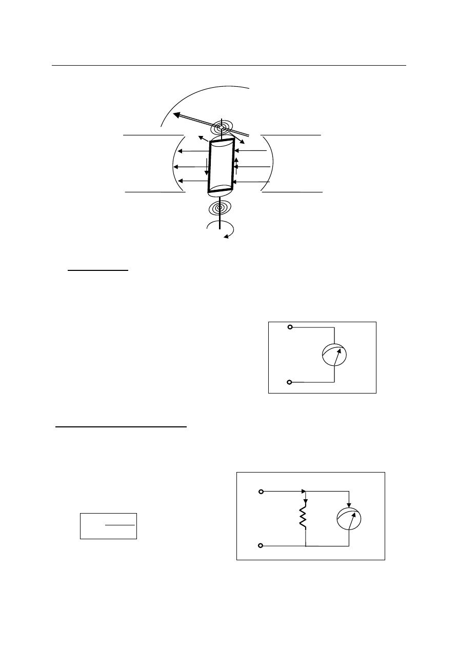
Permanent Magnet Moving Coil Mechanism (PMMC)
In PMMC meter or (D’Arsonval) meter or galvanometer all are the same instrument, a
coil of fine wire is suspended in a magnetic field produced by permanent magnet. According to
the fundamental law of electromagnetic force, the coil will rotate in the magnetic field when it
carries an electric current by electromagnetic (EM) torque effect. A pointer which attached the
movable coil will deflect according to the amount of current to be measured which applied to the
coil. The (EM) torque is counterbalance by the mechanical torque of control springs attached to
the movable coil also. When the torques are balanced the moving coil will stopped and its angular
deflection represent the amount of electrical current to be measured against a fixed reference,
called a scale. If the permanent magnet field is uniform and the spring linear, then the pointer
deflection is also linear.
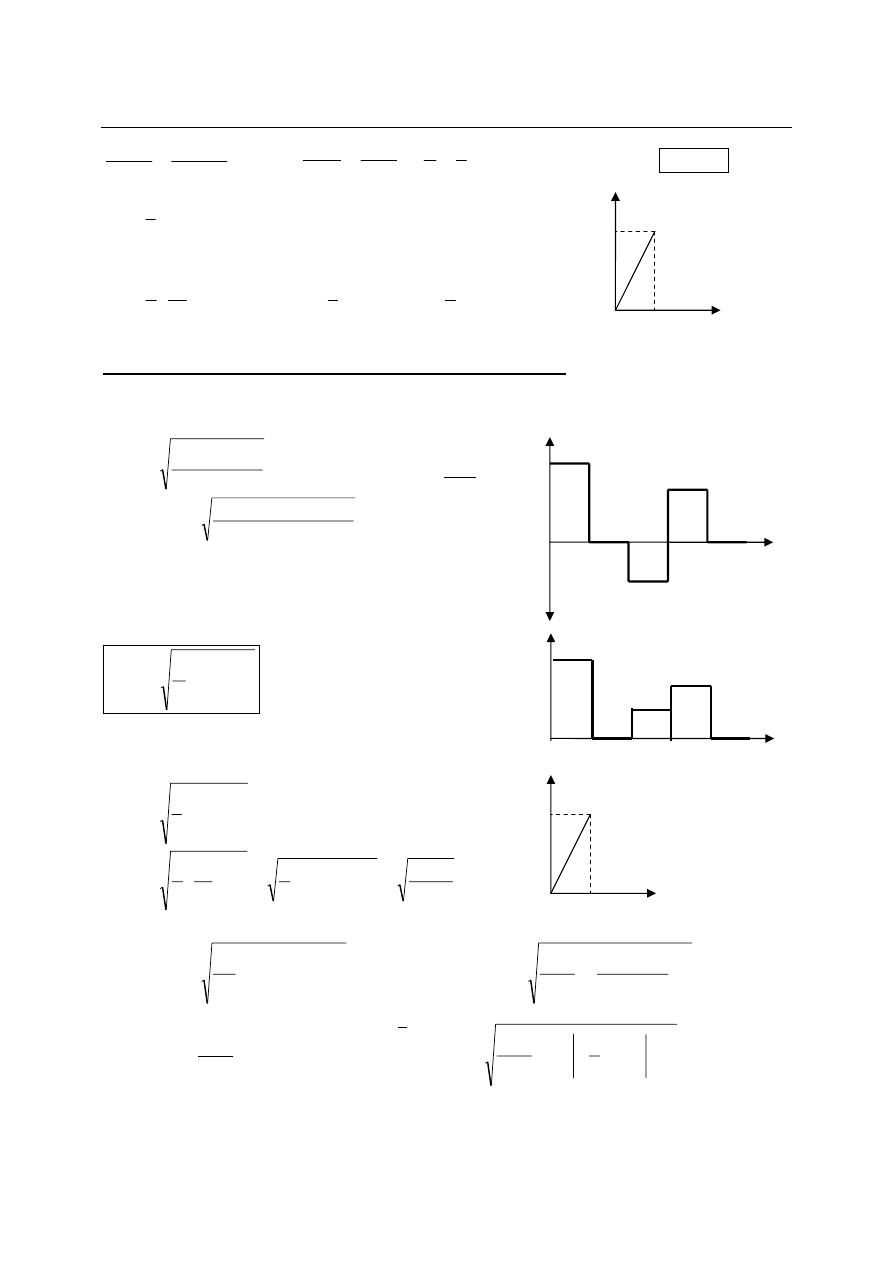
Mathematical Representation of PMMC Mechanism
Assume there are (N) turns of wire and the coil is (L) in long by (W) in wide. The force
(F) acting perpendicular to both the direction of the current flow and the direction of magnetic
field is given by:
L
I
B
N
F
⋅
⋅
⋅
=
where N: turns of wire on the coil I: current in the movable coil
B: flux density in the air gap L: vertical length of the coil
Electromagnetic torque is equal to the multiplication of force with distance to the point of
suspension
2
1
W
NBIL
T
I
=
in one side of cylinder
2
2
W
NBIL
T
I
=
in the other side of cylinder
The total torque for the two cylinder sides
NBIA
NBILW
W
NBIL
T
I
=
=
⎟
⎠
⎞
⎜
⎝
⎛
=
2
2
where A: effective coil area
This torque will cause the coil to rotate until an equilibrium position is reached at an angle θ with
its original orientation. At this position
Electromagnetic torque = control spring torque
T
I
= Ts
Since Ts = Kθ
So
I
K
NBA
=
θ
where
K
NBA
C
=
Thus
CI
=
θ
The angular deflection proportional linearly with applied current
Seventh Lecture Moving Coil Instruments
2
1-
D.c Ammeter:
An Ammeter is always connected in series with a circuit branch and measures the current
flowing in it. Most d.c ammeters employ a d’Arsonval movement, an ideal ammeter
would be capable of performing the measurement without changing or distributing the
current in the branch but real ammeters would possess some internal resistance.
Extension of Ammeter Range:
Since the coil winding in PMMC meter is small and light, they can carry only small
currents (μA-1mA). Measurement of large current requires a shunt external resistor to
connect with the meter movement, so only a fraction of the total current will passes
through the meter.
Vsh
Vm
=
IshRsh
Rm
=
Im
Im
−
=
T
I
Ish
Im
Im
−
=
T
I
Rm
Rsh
S
N
B
B
F
F
pointer
I
I
L
W
Rm
Im
+
-
Rm
Im
+
_
Rsh
Ish
I
range
=I
T
Seventh Lecture Moving Coil Instruments
3
Example:
If PMMC meter have internal resistance of 10Ω and full scale range of 1mA.
Assume we wish to increase the meter range to 1A.
Sol.
So we must connect shunt resistance with the PMMC meter of
Im
Im
−
=
T
I
Rm
Rsh
Ω
=
×
−
⋅
×
=
−
−
01001
.
0
10
1
1
10
10
1
3
3
Rsh
a) Direct D.c Ammeter Method (Ayrton Shunt):
The current range of d.c ammeter can be further extended by a number of shunts selected
by a range switch; such ammeter is called a multirange ammeter.
Im
Im
−
=
∗
∗
Ir
Rm
Rsh
b) Indirect D.C Ammeter Method:
∗
∗
+
=
r
R
Rm
Ir
Im
Where R=Ra+ Rb+ Rc
And r = parallel resistors
branch with the meter
Rm
Im
+
_
Rsh1
Ish1
I
range1
Rsh2
Rsh3
Ish2
Ish3
I
range3
I
range2
Rm
Im
+
_
Ra
Ir1
Ir2
Ir3
Rb
Rc
Seventh Lecture Moving Coil Instruments
4
Example (1):
Design a multirange ammeter by using direct method to give the following ranges 10mA,
100mA, 1A, 10A, and 100A. If d’Arsonval meter have internal resistance of 10Ω and full
scale current of 1mA.
Sol:
Rm=10Ω Im=1mA
Im
Im
−
=
∗
∗
Ir
Rm
Rsh
(
)
Ω
=
×
−
⋅
×
=
−
−
11
.
1
10
1
10
10
10
1
1
3
3
Rsh
(
)
Ω
=
×
−
⋅
×
=
−
−
101
.
0
10
10
100
10
10
1
2
3
3
Rsh
Ω
=
×
−
⋅
×
=
−
−
0101
.
0
10
10
1
10
10
1
3
3
3
Rsh
Ω
=
×
−
⋅
×
=
−
−
0011
.
0
10
1
10
10
10
1
4
3
3
Rsh
Ω
=
×
−
⋅
×
=
−
−
00011
.
0
10
1
100
10
10
1
5
3
3
Rsh
Example (2):
Design an Ayrton shunt by indirect method to provide an ammeter with current ranges
1A, 5A, and 10A, if PMMC meter have internal resistance of 50Ω and full scale current of 1mA.
Sol.:
Rm=50Ω I
FSD
=Im=1mA
∗
∗
+
=
r
R
Rm
Ir
Im
Where R=Ra+ Rb+ Rc
And r = parallel resistors
branch with the meter
1-
For 1A Range:
R
R
Rm
I
+
=
Im
1
+
Rm
Im
_
Rsh1
10mA
Rsh2
Rsh3
1A
100mA
Rsh4
Rsh5
10Ω
100A
1mA
Rm
Im
+
_
Ra
1A
5A
10A
Rb
Rc
Seventh Lecture Moving Coil Instruments
5
R
R
mA
A
+
=
50
1
1
R=0.05005Ω
2-
For 5A Range:
Rc
Rb
R
Rm
I
+
+
=
Im
2
r =Rb+Rc
Rc
Rb
mA
A
+
+
=
05005
.
0
50
1
5
Rb+Rc= 0.01001Ω
Ra=R-(Rb+Rc)
Ra=0.05-0.01001=0.04004 Ω
3-
For 10A Range:
Rc
R
Rm
I
+
=
Im
3
r =Rc
Rc
mA
A
05005
.
0
50
1
10
+
=
Rc=5.005x10
-3
Ω
Rb=0.01001-5.005x10
-3
= 5.005x10
-3
Ω
2-
D.C Voltmeter:
A voltmeter is always connect in parallel with the element being measured, and measures
the voltage between the points across which its’ connected. Most d.c voltmeter employ PMMC
meter with series resistor as shown. The series resistance should be much larger than the
impedance of the circuit being measured, and they are usually much larger than Rm.
Rm
V
Rs
Rm
R
Rs
range
T
−
=
−
=
Im
Im=I
FSD
The ohm/volt sensitivity of a voltmeter
Is given by:
rating
V
I
V
Rm
S
FSD
FSD
v
Ω
=
=
=
1
V
I
V
Rs
Rm
S
Range
Range
Range
Ω
=
=
+
=
1
So the internal resistance of voltmeter or the input resistance of voltmeter is
Rv= V
FSD
x sensitivity
Example:
We have a micro ammeter and we wish to adapted it so as to measure 1volt full scale, the meter
has internal resistance of 100Ω and I
FSD
of 100μA.
Rm
Im
+
_
Rs
V
Range
Seventh Lecture Moving Coil Instruments
6
Sol.:
Rm
V
Rs
−
=
Im
Ω
=
Ω
=
−
=
K
Rs
9
.
9
9900
100
0001
.
0
1
So we connect with PMMC meter a series resistance of 9.9KΩ to convert it to voltmeter
Extension of Voltmeter Range:
Voltage range of d.c voltmeter can be further extended by a number of series resistance
selected by a range switch; such a voltmeter is called multirange voltmeter.
a) Direct D.c Voltmeter Method:
In this method each series resistance of multirange voltmeter is connected in direct with
PMMC meter to give the desired range.
Rm
V
Rs
−
=
∗
∗
Im
b) Indirect D.c Voltmeter Method:
In this method one or more series resistances of multirange voltmeter is connected with
PMMC meter to give the desired range.
Rm
V
Rs
−
=
Im
1
1
Im
1
2
2
V
V
Rs
−
=
Im
2
3
3
V
V
Rs
−
=
Example (1):
A basic d’Arsonval movement with internal resistance of 100Ω and half scale current
deflection of 0.5 mA is to be converted by indirect method into a multirange d.c voltmeter with
voltages ranges of 10V, 50V, 250V, and 500V.
Sol:
I
FSD
= I
HSD
x 2
I
FSD
= 0.5mA x 2 =1mA
Rm
V
Rs
−
=
Im
1
1
Ω
=
−
=
K
mA
Rs
9
.
9
100
1
10
1
Rm
Im
+
_
Rs1
V1
V2
V3
o/p of voltmeter
Rs2
Rs3
Rm
Im
+
_
Rs1
V1
V2
V3
O/P
Rs2
Rs3
Seventh Lecture Moving Coil Instruments
7
Im
1
2
2
V
V
Rs
−
=
Ω
=
×
−
=
−
K
Rs
40
10
1
10
50
2
3
Ω
=
×
−
=
−
K
Rs
200
10
1
50
250
3
3
Ω
=
×
−
=
−
K
Rs
250
10
1
250
500
4
3
Example (2):
Design d.c voltmeter by using direct method with d’Arsonval meter of 100Ω and full
scale deflection of 100μA to give the following ranges: 10mV, 1V, and 100V.
Sol:
Rm
V
Rs
−
=
∗
∗
Im
Rm
V
Rs
−
=
Im
1
1
Ω
=
−
=
0
100
100
10
1
A
mV
Rs
μ
Ω
=
−
×
=
−
K
Rs
9
.
9
100
10
100
1
2
6
Ω
=
−
×
=
−
K
Rs
9
.
99
100
10
100
100
3
6
3-
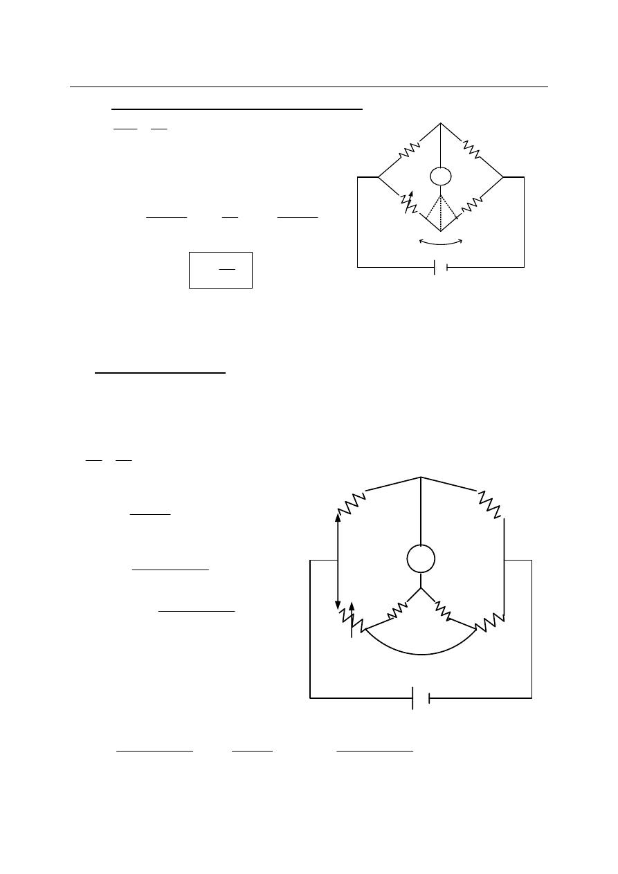
Ohmmeter and Resistance measurement:
When a current of 1A flows through a circuit which has an impressed voltage of 1volt, the
circuit has a resistance of 1Ω.
I
V
R
=
There are several methods used to measure unknown resistance:
a) Indirect method by ammeter and voltmeter.
This method is inaccurate unless the ammeter has a small resistance and voltmeter have a
high resistance.
Rm
Im
+
_
Rs1
10V
50V
250V
O/P
Rs2
Rs3
Rs4
500V
Rm
Im
+
_
Rs1
100mV
1V
100V
o/p of voltmeter
Rs2
Rs3
Seventh Lecture Moving Coil Instruments
8
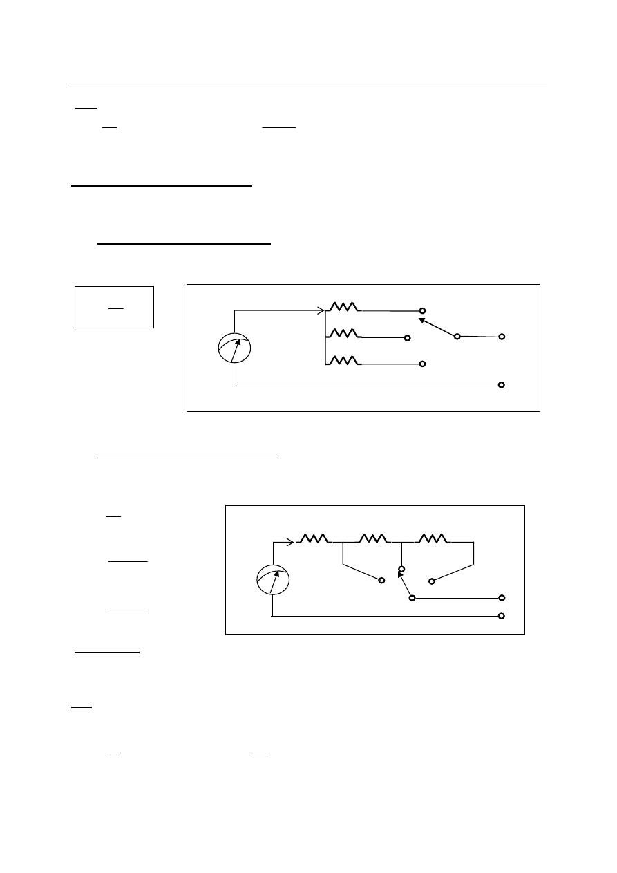
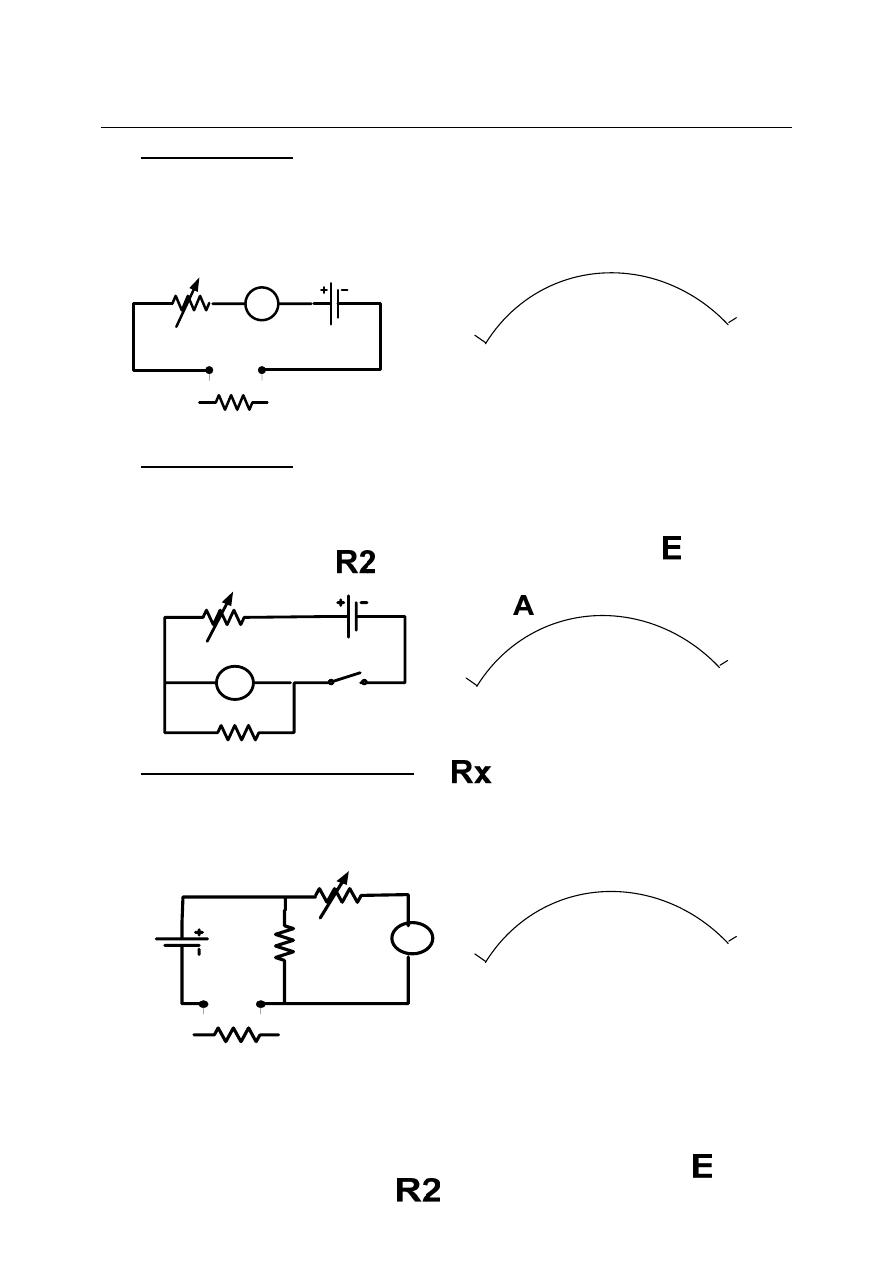
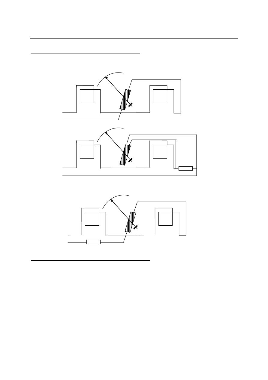
b) Series Ohmmeter:
Rx is the unknown resistor to be measured, R2 is variable adjusted resistance so that
the pointer read zero at short circuit test. The scale of series ohmmeter is nonlinear with
zero at the right and infinity at extreme left. Series ohmmeter is the most generally used
meter for resistance measurement.
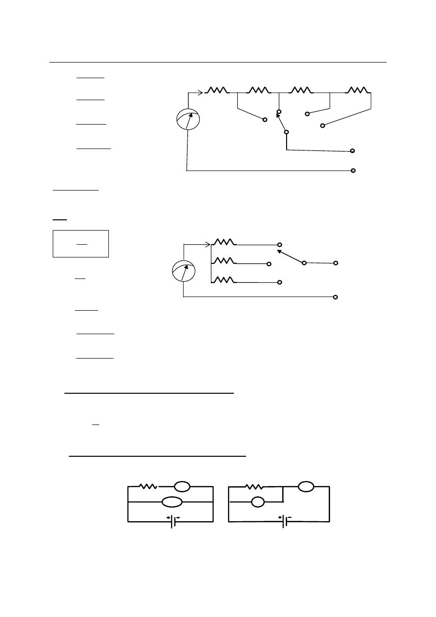
c) Shunt Ohmmeter:
Shunt ohmmeter are used to measure very low resistance values. The unknown
resistance Rx is now shunted across the meter, so portion of current will pass across this
resistor and drop the meter deflection proportionately. The switch is necessary in shunt
ohmmeter to disconnect the battery when the instrument is not used. The scale of shunt
ohmmeter is nonlinear with zero at the left and infinity at extreme right.
d) Voltage Divider (potentiometer):
The meter of voltage divider is voltmeter that reads voltage drop across Rs which
dependent on Rx. This meter will read from right to left like series ohmmeter with more
uniform calibration.
∞
0
∞
0
∞
0
Eighth Lecture A.c Measuring Instruments
1
A.c Measuring Instrument
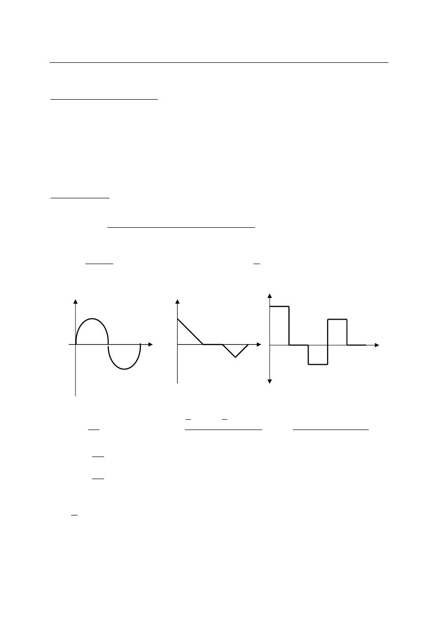
Review on Alternating Signal:
The instantaneous values of electrical signals can be graphed as they vary with time. Such
graphs are known as the waveforms of the signal. If the value of waveform remains constant with
time, the signal is referred to as direct (d.c) signal; such as the voltage of a battery. If a signal is
time varying and has positive and negative instantaneous values, the waveform is known as
alternating (a.c) waveform. If the variation of a.c signal is continuously repeated then the signal
is known as periodic waveform.
The frequency of a.c signal is defined as the number of cycles traversed in one second. Thus
the time duration of one cycle per second for a.c signal is known as the period (T). Where the
complete variation of a.c signal before repeated itself is represent one cycle.
Average Values:
It is found by dividing the area under the curve of the waveform in one period (T) by the
time of the period.
Average value= Algebraic sum of the areas under the curve
Length of the curve
T
areas
Av
∑
=
…………….. (1) or
∫
=
T
dt
t
f
T
Av
0
)
(
1
…………….. (2)
∫
=
π
θ
θ
π
2
0
2
1
d
VmSin
Av
( )
9
3
4
2
1
6
3
2
1
−
×
×
+
×
×
=
Av
( )
10
2
3
2
2
2
4
×
+
×
−
+
×
=
Av
(
)
π
θ
π
2
0
2
↑
−
=
Cos
Vm
Av
( )
0
1
1
2
=
−
−
=
π
Vm
Av
The average value for the figure below by using equation (2) is:
∫
=
T
dt
t
f
T
Av
0
)
(
1
we use the tangent equation for (xo,yo)=(0,0), and (x
1
,y
1
)=(3,6) to find the
function of f(t)
2
4
6
8
10
-2
3
4
V
t
t
7 9
5
3
6
-3
V
2Π
Π
0
θ
Vm
V
Eighth Lecture A.c Measuring Instruments
2
1
2
1
2
1
1
x
x
y
y
x
x
y
y
−
−
=
−
−
→
x
y
x
y
x
y
2
2
3
6
0
3
0
6
0
0
=
⇒⇒
=
=
⇒
−
−
=
−
−
t
t
f
2
)
(
=
( )
∫
=
3
0
2
3
1
dt
t
Av
⎟
⎟
⎠
⎞
⎜
⎜
⎝
⎛
↑
=
3
0
2
2
3
2 t
Av
( ) ( )
(
)
3
3
9
0
3
3
1
2
2
=
=
−
=
Av
Root Mean Square Value(effective value of a.c signal):
The r.m.s value of a waveform refers to its power capability. It is refer to the effective
value of a.c signal because the r.m.s value equal to the value of a d.c signal which would deliver
the same power if it replaced with a.c signal.
T
V
area
s
m
r
∑
=
2
)
(
.
.
( for square waveform only)
1-
10
2
9
2
4
2
16
.
.
×
+
×
+
×
=
s
m
r
In general form the r.m.s value has the following aqua.
r.m.s= √Average f(t)
2
dt
t
f
T
s
m
r
T
∫
=
0
2
)
(
1
.
.
2-
If f(t) = 2t then its r.m.s value is:
( )
∫
=
3
0
2
2
3
1
.
.
dt
t
s
m
r
( ) ( )
(
)
46
.
3
9
27
4
0
3
9
4
3
3
4
.
.
3
3
3
0
3
=
×
=
−
=
⎟
⎟
⎠
⎞
⎜
⎜
⎝
⎛
↑
=
t
s
m
r
3-
If f(t) = Vm Sinθdθ
∫
=
π
θ
θ
π
2
0
2
2
2
1
.
.
d
Sin
Vm
s
m
r
∫
−
=
π
θ
θ
π
2
0
2
2
2
1
2
.
.
d
Cos
Vm
s
m
r
2
1
2
0
2
0
2
2
4
.
.
⎪⎭
⎪
⎬
⎫
⎪⎩
⎪
⎨
⎧
⎥
⎥
⎦
⎤
⎢
⎢
⎣
⎡
−
=
∫
∫
π
π
θ
θ
θ
π
d
Cos
d
Vm
s
m
r
⎥
⎥
⎦
⎤
⎢
⎢
⎣
⎡
−
=
π
π
θ
θ
π
2
0
2
0
2
2
2
1
4
.
.
Sin
Vm
s
m
r
3
6
(3,6)
(0,0)
f(t)
t
2
4
6
8
10
-2
3
4
V
t
2
4
6
8
10
9
16
V
2
t
4
3
6
(3,6)
(0,0)
f(t)
t
Eighth Lecture A.c Measuring Instruments
3
[
]
2
2
0
2
4
.
.
2
2
Vm
Vm
Vm
s
m
r
=
=
−
=
π
π
average
s
m
r
FormFactor
.
.
=
for Sine wave F.F=1.11 (F.W.R)
F.F=1.57 (H.W.R)
s
m
r
PeakValue
r
CrestFacto
.
.
=
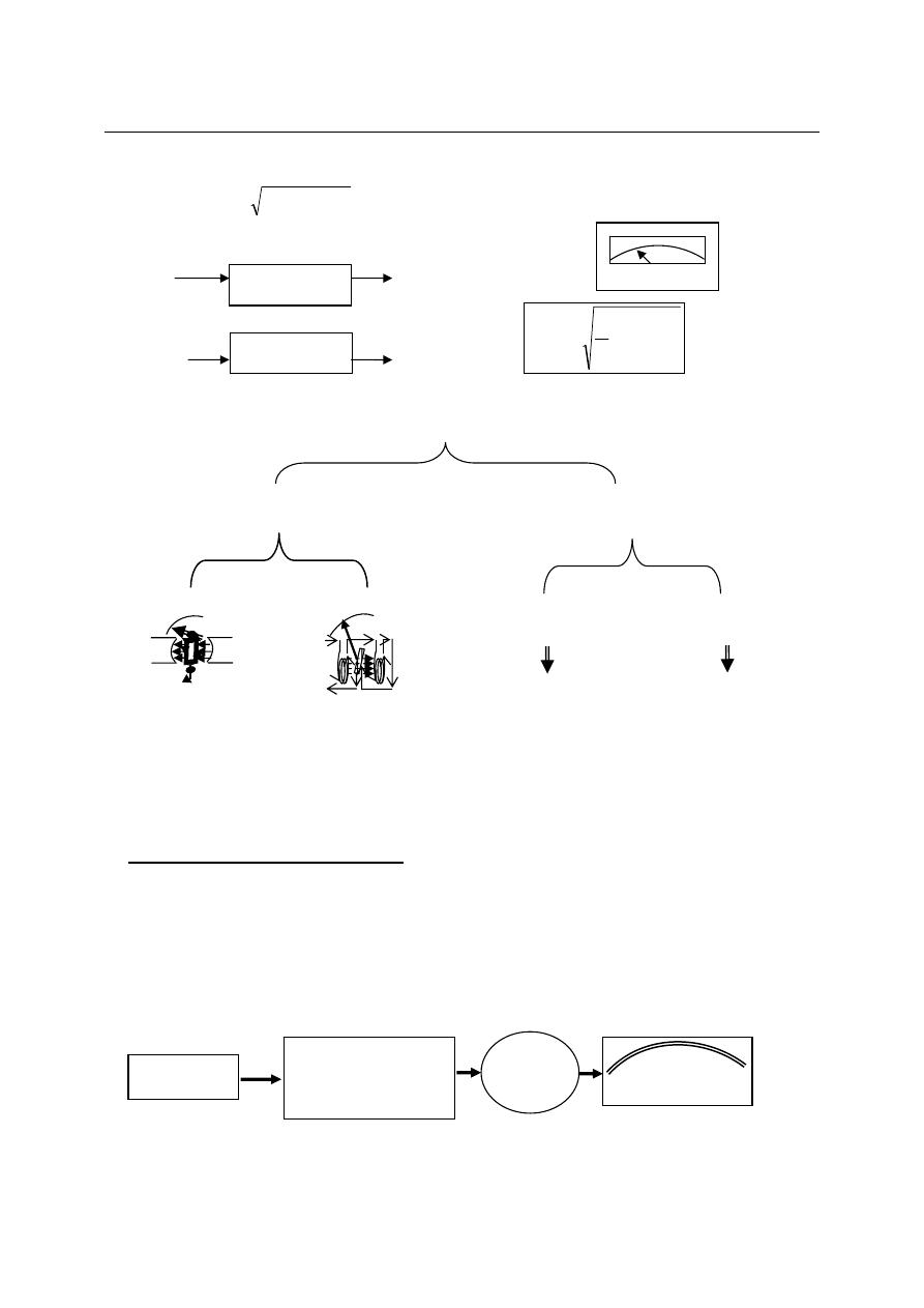
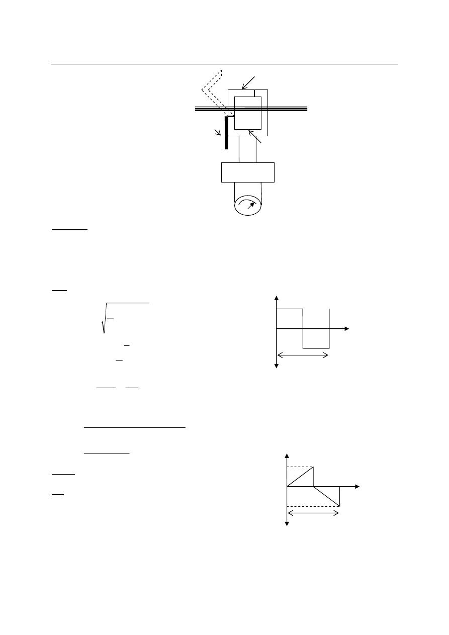
Dynamometer:
This instrument is suitable for the measurement of direct and alternating current, voltage
and power. The deflecting torque in dynamometer is relies by the interaction of magnetic field
produced by a pair of fixed air cored coils and a third air cored coil capable of angular movement
and suspended within the fixed coil.
A
i
B
N
T
m
i
=
,
f
i
B
α
thus
⇒⇒
A
i
i
T
f
m
i
α
so
2
i
T
i
α
θ α average i
2
, since
2
)
(
.
.
t
averagef
s
m
r
=
2Π
Π
0
θ
Vm
V
Fixed
coil
Fixed
coil
moving
coil
pointer
Non linear scale
FSD
0
N
N
N
S
S
S
FSD
0
i
i
N
N
N
S
S
S
i
i
FSD
0
Eighth Lecture A.c Measuring Instruments
4
The output scale is calibrated to give the r.m.s value of a.c signal by taking the square roots of
the inside measured value.
O/P scale =
2
)
(
.
.
i
average
s
m
r
=
, for example if (average i
2
) = 16 inside the measuring device,
the output scale of the device will indicate (4)
dt
t
f
T
s
m
r
T
∫
=
0
2
)
(
1
.
.
1-
Average Responding a.c Meter:
O/P (r.m.s) = Av x F.F
sine wave
F.F
sine wave
(F.W.R) = 1.11
(measured) F.F
sine wave
(H.W.R) = 1.57
O/P (r.m.s) = Av x F.F
true
F.F
true
= The form factor of any input signal
(true) (sine, square, or any thing)
4
dynamometer
dynamometer
d.c
d.c
a.c
r.m.s
Meters
d.c meters
measure d.c or Av values
a.c meters
measure r.m.s values
PMMC
dynamometer
Average Responding
a.c meter
True Responding
a.c meter
Rectifier + PMMC
dynamometer
T α i
2
B varied
non linear
scale
θα average i
2
T α i
B constant
linear scale
θα i
Rectifier circuit
To remove the negative
part
PMMC
Measure
Av.
Scale calibrated by
O/P=Av x F.F
sine
a.c i/p
signal
Eighth Lecture A.c Measuring Instruments
5
2-
True Responding a.c Meter (Dynamometer):
O/P (r.m.s) = Av x F.F
true
F.F
true
= The form factor of any input signal
(true) = (measured)
Example:
What will be the out put of the following meters, if an average responding a.c meter of half-
wave rectifier read (4.71v), and true form factor of input waveform is (1.414).
Sol:
Av
s
m
r
measured
×
= 57
.
1
.
.
for average responding a.c meter of half wave rectifier
Av
×
= 57
.
1
71
.
4
V
Av
3
57
.
1
71
.
4
=
=
⇒
1. D’Arsonval meter read Av = 3V
2. HWR+PMMC (Average responding of halve wave rectifier) meter = 4.71V
3. FWR+PMMC (Average responding of full wave rectifier) meter = 1.11 x 3 = 3.33V
4. Dynamometer =F.F
(true)
x Av
r.m.s
(true)
= 1.414 x 3 = 4.242V
Exercise: What will be the o/p of the following meters?
I/P a.c
signal
Dynamometer
O/P
r.m.s
F.W.R
+
PMMC
meter
D’Arsonval
meter
H.W.R
+
PMMC
meter
Dynamo.
meter
1
2
3
4
F.W.R
+
PMMC
meter
D’Arsonval
meter
H.W.R
+
PMMC
meter
Dynamo.
meter
1
2
3
4
R
E=10V
Eighth Lecture A.c Measuring Instruments
6
Dynamometer As Ammeter And Voltmeter:
For small current measurement (5mA to 100mA), fixed and moving coils are connect in
series. While larger current measurement (up to 20A) , the moving coil is shunted by a small
resistance.
To convert such an instrument to a voltmeter only a rather big series resistance is connected with
the moving coil.
Clamp on Meters
(Average Responding A.C meter)
:
One application of average responding a.c meters is the clamp on meter which is used to
measured a.c current, voltage in a wire with out having to break the circuit being measured.
The meter having use the transformer principle to detect the current. That is, the clamp on device
of the meter serves as the core of a transformer. The current carrying wire is the primary winding
of the transformer, while the secondary winding is in the meter. The alternating current in the
primary is coupled to the secondary winding by the core, and after being rectified the current is
sensed by a d’Arsonval meter.
Fixed
Fixed
moving
Rs
Fixed
Fixed
moving
Fixed
Fixed
moving
Rsh
Eighth Lecture A.c Measuring Instruments
7
Example:
The symmetrical square wave voltage is applied to an average responding a.c voltmeter with a
scale calibrated in term of the r.m.s value of a sine wave. Calculate:
1. The form factor of square wave voltage.
2. The error in the meter indication.
Sol:
Vm
dt
t
V
T
Vrms
T
o
True
=
=
∫
2
)
(
)
(
1
Vm
dt
t
V
T
Vaverage
T
o
True
=
=
∫
2
)
(
)
(
2
1
.
.
)
(
=
=
=
Vm
Vm
Vav
Vrms
F
F
True
Vm
Vm
Av
Vrms
measured
11
.
1
11
.
1
.
11
.
1
)
(
=
×
=
×
=
%
100
)
(
)
(
)
(
×
−
=
True
measured
True
Vrms
Vrms
Vrms
Error
%
100
11
.
1
×
−
=
Vm
Vm
Vm
Error
Exer.:
Repeat the above example for saw tooth waveform shown
Sol:
V(t)=25t
Vav.=50V
Vrms
(True)
=57.75V
Vrms
(Measured)
=55.5V
F.F
(True)
=1.154
Error=0.0389%
Rectifier
PMMC
Secondary
Winding
Current carrying
conductor
Core
As primary
winding
Mechanism
For opening
clamp on meter
T
-Vm
Vm
t
V(t)
4Sec
-100
100
t
V(t)
Ninth Lecture Bridges and Their Application
1
Bridges and Their Application
Bridge circuit are extensively used for measuring component values, such as resistance,
inductance, capacitance, and other circuit parameters directly derived from component values
such as frequency, phase angle, and temperature. Bridge accuracy measurements are very high
because their circuit merely compares the value of an unknown component to that of an
accurately known component (a standard).
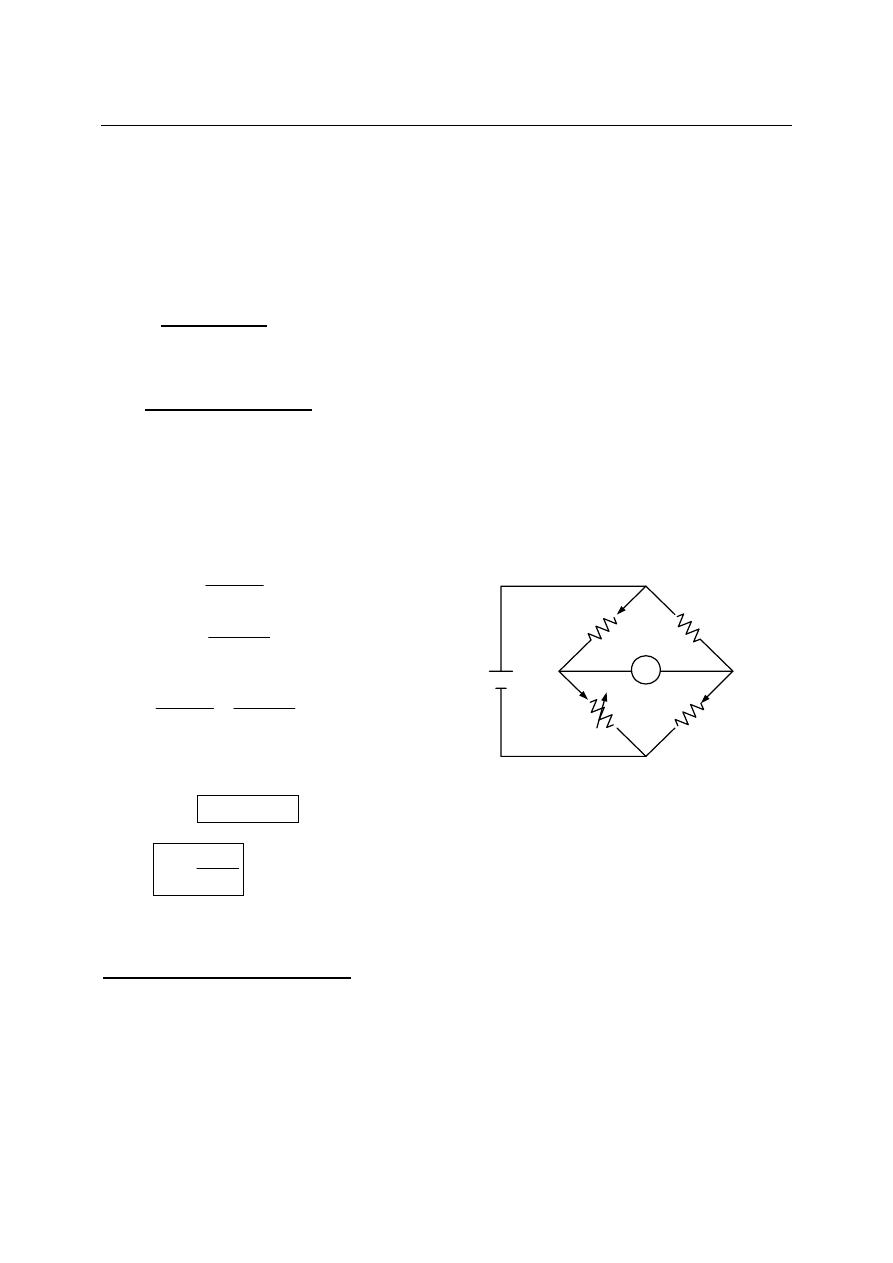
1- D.c Bridges:
The basic d.c bridges consist of four resistive arms with a source of emf (a battery) and a
null detector usually galvanometer or other sensitive current meter. D.c bridges are generally
used for the measurement of resistance values.
a) Wheatstone Bridge:
This is the best and commonest method of measuring medium resistance values in the
range of 1Ω to the low megohm. The current through the galvanometer depends on potential
difference between point (c) and (d). The bridge is said to be balance when potential
difference across the galvanometer is zero volts, so there is no current through the
galvanometer (Ig=0). This condition occurs when Vca=Vda or Vcb=Vdb hence the
bridge is balance when
2
1 V
V
=
…….. (1) Since
0
=
g
I
so by voltage divider rule
3
1
1
1
R
R
R
E
V
+
=
….. (2) and
4
2
2
2
R
R
R
E
V
+
=
….. (3)
Substitute equations (2) & (3) in equ. (1)
4
2
2
3
1
1
R
R
R
R
R
R
+
=
+
Thus
3
2
4
1
R
R
R
R
=
is the balance equation for Wheatstone bridge
So, if three of resistance values are known, the fourth unknown ones can be determined.
1
2
3
4
R
R
R
R
=
R
3
are called the standard arm of the bridge and resistors R
2
and R
1
are called the ratio
arms.
Thevenin Equivalent Circuit:
To determine whether or not the galvanometer has the required sensitivity to detect an
unbalance condition, it is necessary to calculate the galvanometer current for small unbalance
condition. The solution is approached by converting the Wheatstone bridge to its thevenin
equivalent. Since we are interested in the current through the galvanometer, the thevenin
equivalent circuit is determined by looking into galvanometer terminals (c) and (d).
R
1
R
3
R
2
R
4
G
E
a
b
c
d
I
1
I
2
I
3
I
4
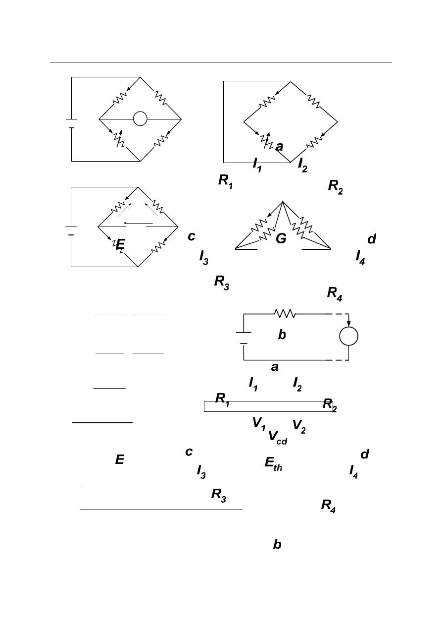
Ninth Lecture Bridges and Their Application
2
when
0
=
E
4
2
4
2
3
1
3
1
R
R
R
R
R
R
R
R
Rth
+
+
+
=
2
1
V
V
E
th
−
=
0
≠
E
4
2
2
3
1
1
R
R
ER
R
R
ER
E
th
+
−
+
=
Rg
Rth
E
Ig
th
+
=
and galvanometer deflection (d) is: d = Ig x current sensitivity (mm/μA)
b) Kelvin Bridge:
Kelvin bridge is a modification of the Wheatstone bridge and provides greatly increased
accuracy in the measurement of low value resistance, generally below (1Ω). It is eliminate
errors due to contact and leads resistance. (Ry) represent the resistance of the connecting
lead from R
3
to R
4
. Two galvanometer connections are possible, to point (m) or to point
(n).
1-
If the galvanometer connect to point (m) then
y
x
R
R
R
+
=
4
therefore unknown resistance will be higher than its actual value by R
y
2-
If the galvanometer connect to point (n) then
y
R
R
R
+
=
3
4
therefore unknown resistance will be lower than its actual value by R
y
a
R
1
R
3
R
2
R
4
c
d
R
th
E
th
R
th
G
c
d
R
g
I
g
Ninth Lecture Bridges and Their Application
3
3-
If the galvanometer connect to point (p) such that
2
1
R
R
R
R
mp
np
=
………. (1)
At balance condition
(
) (
)
mp
np
x
R
R
R
R
R
R
+
=
+
3
1
2
…….. (2)
Substituting equ.(1) in to equ.(2) we obtain
⎥
⎦
⎤
⎢
⎣
⎡
⎟⎟
⎠
⎞
⎜⎜
⎝
⎛
+
+
=
⎟⎟
⎠
⎞
⎜⎜
⎝
⎛
+
+
y
y
x
R
R
R
R
R
R
R
R
R
R
R
R
2
1
2
3
2
1
2
1
1
This reduces to
3
2
1
R
R
R
R
x
=
So the effect of the resistance of the connecting lead from point (m) to point (n) has be
eliminated by connecting the galvanometer to the intermediate position (p).
c) Kelvin Double Bridge:
Kelvin double bridge is used for measuring very low resistance values from approximately
(1Ω to as low as 1x10
-5
Ω). The term double bridge is used because the circuit contains a second
set of ratio arms labelled Ra and Rb. If the galvanometer is connect to point (p) to eliminates
the effect of (yoke resistance Ry).
2
1
R
R
R
R
b
a
=
At balance
b
V
V
V
+
=
3
2
………. (1)
2
1
2
2
R
R
R
E
V
+
=
……….. (2)
3
3
3
R
I
V
=
and
b
b
b
R
I
V
=
….. (3)
(
)
y
y
b
R
Rb
Ra
R
I
I
+
+
=
3
………… (4)
(
)
(
)
⎥
⎥
⎦
⎤
⎢
⎢
⎣
⎡
+
+
+
+
+
=
4
3
3
R
R
Rb
Ra
R
Rb
Ra
R
I
E
y
y
… (5)
Sub.equ. (5) in to equ. (2) and equ. (4)
into equ.(3) then substitute the result in
equ.(1), we get
(
)
(
)
⎥
⎥
⎦
⎤
⎢
⎢
⎣
⎡
+
+
+
+
+
4
3
3
R
R
Rb
Ra
R
Rb
Ra
R
I
y
y
2
1
2
R
R
R
+
3
3
R
I
=
(
)
y
y
R
Rb
Ra
R
I
+
+
+
3
b
R
R
1
R
3
R
2
R
4
G
E
n
p
m
R
y
R
1
R
3
R
2
R
4
G
E
n
p
m
R
y
L
K
O
R
a
R
b
I
2
I
3
I
b
Ninth Lecture Bridges and Their Application
4
⎥
⎦
⎤
⎢
⎣
⎡
−
−
+
+
+
+
=
Rb
Ra
R
R
R
Rb
Ra
Rb
R
R
R
R
R
y
y
x
1
1
2
1
2
1
3
⎥
⎦
⎤
⎢
⎣
⎡
−
+
+
+
=
Rb
Ra
R
R
R
Rb
Ra
Rb
R
R
R
R
R
y
y
x
2
1
2
1
3
This is the balanced equation
If
2
1
R
R
R
R
b
a
=
then
2
1
3
R
R
R
R
x
=
2-
Ac Bridge and Their Application:
The ac bridge is a natural outgrowth of the dc bridge and in its basic form consists of four
bridge arms, a source of excitation, and a null ac detector. For measurements at low
frequencies, the power line may serve as the source of excitation; but at higher frequencies an
oscillator generally supplies the excitation voltage. The null ac detector in its cheapest
effective form consists of a pair of headphones or may be oscilloscope.
The balance condition is reached when
the detector response is zero or indicates
null. Then V
AC
= 0 and V
Z1
= V
Z2
3
1
1
1
Z
Z
Z
Vin
V
Z
+
=
4
2
2
2
Z
Z
Z
Vin
V
Z
+
=
thus
3
2
4
1
Z
Z
Z
Z
=
is the balance equation
Or
3
2
4
1
Y
Y
Y
Y
=
The balance equation can be written in complex form as:
(
)(
) (
)
(
)
3
3
2
2
4
4
1
1
θ
θ
θ
θ
∠
∠
=
∠
∠
Z
Z
Z
Z
And
(
)
(
)
3
2
3
2
4
1
4
1
θ
θ
θ
θ
+
∠
=
+
∠
Z
Z
Z
Z
So two conditions must be met simultaneously when balancing an ac bridge
1-
3
2
4
1
Z
Z
Z
Z
=
2-
4
2
4
1
θ
θ
θ
θ
∠
+
∠
=
∠
+
∠
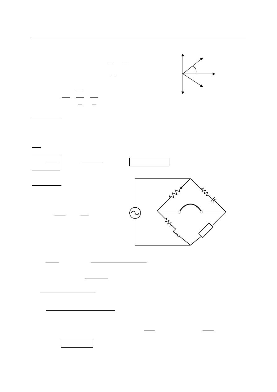
Review on Ac Impedance:
a) In series connection
Impedance = resistance ± j reactance
jXL
R
Z
L
+
=
and
L
j
R
Z
L
ω
+
=
jXC
R
Z
C
−
=
and
C
j
R
Z
C
ω
1
−
=
Conversion from polar to rectangular
θ
∠
Z
in polar form R= Z Cosθ X= Z Sinθ become
jX
R
Z
±
=
Conversion from rectangular to polar
jX
R
Z
±
=
in rectangular form
2
2
X
R
Z
+
=
R
X
1
tan
−
=
θ
R
X
=
θ
tan
Z
1
Z
3
Z
2
Z
4
V
in
A
B
C
D
i
1
i
2
i
3
i
4
Z
Z
Z
Z
R
jXL
-jXC
Z
L
Ninth Lecture Bridges and Their Application
5
b)
In parallel connection
Admittance = conductance ± j susceptance
L
L
jB
G
Y
−
=
and
L
j
R
Y
L
ω
1
1 −
=
C
C
jB
G
Y
+
=
and
C
j
R
Y
C
ω
+
=
1
RC
R
C
R
Xc
G
B
C
ω
ω
θ
=
=
=
=
1
1
1
tan
Example (1):
The impedance of the basic a.c bridge are given as follows:
o
80
100
1
∠
=
Z
(inductive impedance)
Ω
250
2
=
Z
o
30
400
3
∠
=
Z
(inductive impedance)
unknown
Z
=
4
Sol:
1
3
2
4
Z
Z
Z
Z
=
Ω
k
Z
1
100
400
250
4
=
×
=
1
3
2
4
θ
θ
θ
θ
−
+
=
o
50
80
30
0
4
−
=
−
+
=
θ
o
50
1000
4
−
∠
=
Z
(capacitive impedance)
Example (2):
For the following bridge find Zx?
The balance equation
3
2
4
1
Z
Z
Z
Z
=
Ω
450
1
=
= R
Z
C
j
R
C
j
R
Z
ω
ω
−
=
+
=
1
2
600
300
2
j
Z
−
=
L
j
R
Z
ω
+
=
3
100
200
3
j
Z
+
=
unknown
Z
Z
x
=
=
4
1
3
2
4
Z
Z
Z
Z
=
(
)(
)
200
6
.
266
450
100
200
600
300
4
j
j
j
Z
−
=
+
−
=
Ω
6
.
266
=
R
F
F
C
μ
π
79
.
0
200
2
1
=
×
=
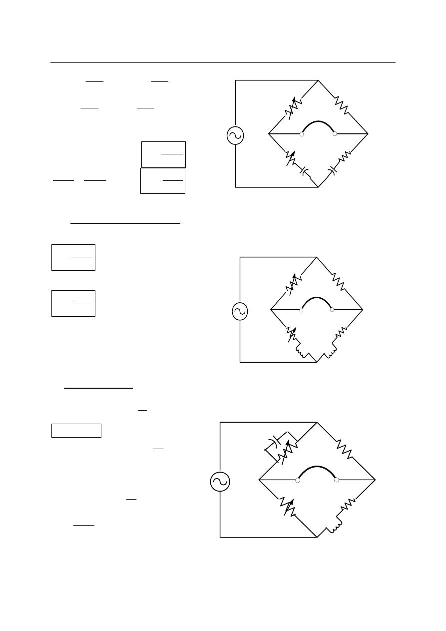
a) Comparison Bridges:
A.c comparison bridges are used to measure unknown inductance or capacitance by
comparing it with a known inductance or capacitance.
1-
Capacitive Comparison Bridge:
In capacitive comparison bridge R1 & R2 are ratio arms, Rs in series with Cs are
standard known arm, and Cx represent unknown capacitance with its leakage resistance Rx.
1
1
R
Z
=
2
2
R
Z
=
s
s
C
j
R
Z
ω
−
=
3
x
x
C
j
R
Z
ω
−
=
4
At balance
3
2
4
1
Z
Z
Z
Z
=
G
jB
C
-jB
L
Y
C
Y
L
Z
1
Z
3
Z
2
V
in
A
B
C
D
Z
x
Z
1V
1KHz
30
0
45
0
0.
26
5
F
20
0
15
.9
m
H
Ninth Lecture Bridges and Their Application
6
⎟⎟
⎠
⎞
⎜⎜
⎝
⎛
−
=
⎟⎟
⎠
⎞
⎜⎜
⎝
⎛
−
s
s
x
x
C
j
R
R
C
j
R
R
ω
ω
2
1
s
s
x
x
C
jR
R
R
C
jR
R
R
ω
ω
2
2
1
1
−
=
−
By equating the real term with the real
and imaginary term with imaginary we get:
s
x
R
R
R
R
2
1
=
1
2
R
R
R
R
s
x
=
s
x
C
jR
C
jR
ω
ω
2
1
−
=
−
2
1
R
C
R
C
s
x
=
We can note that the bridge is independent
on frequency of applied source.
2- Inductive Comparison Bridge:
The unknown inductance is determined by comparing it with a known standard inductor.
At balance we get
1
2
R
R
R
R
s
x
=
represent resistive balance equation
1
2
R
L
R
L
s
x
=
inductive balance equation
b) Maxwell bridge:
This bridge measure unknown inductance in terms of a known capacitance, at balance:
3
2
4
1
Z
Z
Z
Z
=
1
1
1
Y
Z
=
thus
1
3
2
4
Y
Z
Z
Z
=
where
2
2
R
Z
=
3
3
R
Z
=
1
1
1
1
C
j
R
Y
ω
+
=
x
x
L
j
R
Z
ω
+
=
4
So
⎟⎟
⎠
⎞
⎜⎜
⎝
⎛
+
=
+
1
1
3
2
1
C
j
R
R
R
L
j
R
x
x
ω
ω
1
3
2
R
R
R
R
x
=
1
3
2
C
R
R
L
x
=
Z
1
Z
3
Z
2
V
in
A
B
C
D
Z
4
C
x
C
s
R
x
R
s
R
2
R
1
Z
1
Z
3
Z
2
V
in
A
B
C
D
Z
4
L
x
L
s
R
x
R
s
R
2
R
1
Y
1
Z
3
Z
2
V
in
A
B
C
D
Z
4
L
x
R
x
R
2
R
1
C
1
R
3
Ninth Lecture Bridges and Their Application
7
Maxwell bridge is limited to the measurement of medium quality factor (Q) coil with range
between 1<Q≤10
Q
C
R
R
XC
G
B
R
L
c
=
=
=
=
=
=
1
1
1
1
1
1
4
4
4
1
1
1
tan
tan
ω
ω
θ
θ
c) Hay Bridge:
Hay bridge convening for measuring high Q coils
1
1
1
C
j
R
Z
ω
−
=
2
2
R
Z
=
3
3
R
Z
=
x
x
L
j
R
Z
ω
+
=
4
At balance
3
2
4
1
Z
Z
Z
Z
=
(
)
3
2
1
1
R
R
L
j
R
C
j
R
x
x
=
+
⎟⎟
⎠
⎞
⎜⎜
⎝
⎛
−
ω
ω
3
2
1
1
1
1
R
R
L
R
j
C
jR
C
L
R
R
x
x
x
x
=
+
−
+
ω
ω
Separating the real and imaginary terms
3
2
1
1
R
R
C
L
R
R
x
x
=
+
….. (1)
x
x
L
R
C
R
1
1
ω
ω
=
…… … (2)
Solving equ.(1) and (2) yields
2
1
2
1
2
3
2
1
2
1
2
1
R
C
R
R
R
C
R
x
ω
ω
+
=
2
1
2
1
2
1
3
2
1
R
C
C
R
R
L
x
ω
+
=
4
1
θ
θ
−
=
because
zero
=
= 3
2
θ
θ
Q
R
C
R
C
R
XC
R
L
=
=
=
=
=
=
1
1
1
1
1
1
4
4
4
1
1
1
tan
tan
ω
ω
ω
θ
θ
Thus
1
1
1
C
R
Q
ω
=
…….. (3)
Submitted equ.(3) in to equ. (2) yield
2
1
3
2
1
1
⎟⎟
⎠
⎞
⎜⎜
⎝
⎛
+
=
Q
C
R
R
L
x
For Q> 10, then
1
1
2
<<
⎟⎟
⎠
⎞
⎜⎜
⎝
⎛
Q
and can be neglected, then
1
3
2
C
R
R
L
x
=
Z
1
Z
3
Z
2
V
in
A
B
C
D
Z
4
L
x
R
x
R
2
R
1
C
1
R
3
Ninth Lecture Bridges and Their Application
8
d) Schering Bridge:
Schering bridge used extensively for capacitive measurement, (C3) is standard high mica
capacitor for general measurement work, or (C3) may be an air capacitor for insulation
measurements. The balance condition require that
3
2
4
1
θ
θ
θ
θ
+
=
+
but
90
4
1
−
=
+
θ
θ
Thus
3
2
θ
θ
+
must equal (-90) to get balance
At balance
1
3
2
4
Y
Z
Z
Z
=
1
1
1
1
C
j
R
Y
ω
+
=
2
2
R
Z
=
3
3
C
j
Z
ω
−
=
x
x
C
j
R
Z
ω
−
=
4
⎟⎟
⎠
⎞
⎜⎜
⎝
⎛
+
⎟⎟
⎠
⎞
⎜⎜
⎝
⎛ −
=
−
1
1
3
2
1
C
j
R
C
j
R
C
j
R
x
x
ω
ω
ω
1
3
2
2
1
2
R
C
jR
C
C
R
C
j
R
x
x
ω
ω
−
=
−
3
1
2
C
C
R
R
x
=
…… (1)
2
1
3
R
R
C
C
x
=
…… (2)
The power factor (pf):
x
x
c
Z
R
Cos
pf
=
=
θ
The dissipation factor (D):
x
x
x
x
c
C
R
Q
XC
R
Cot
D
ω
θ
=
=
=
=
1
…… (3)
Substitute equs. (1) & (2) into (3), we get
1
1
C
R
D
ω
=
e) Wien Bridge:
This bridge is used to measured
unknown frequency
1
1
1
C
j
R
Z
ω
−
=
2
2
R
Z
=
3
3
3
1
C
j
R
Y
ω
+
=
4
4
R
Z
=
3
2
4
1
Y
Z
Z
Z
=
3
4
1
2
Y
Z
Z
Z
=
⎟⎟
⎠
⎞
⎜⎜
⎝
⎛
+
⎟⎟
⎠
⎞
⎜⎜
⎝
⎛
−
=
3
3
4
1
1
2
1
C
j
R
R
C
j
R
R
ω
ω
1
3
4
3
4
1
2
C
C
R
R
R
R
R
+
=
Dividing by R
4
we get
1
3
3
1
4
2
C
C
R
R
R
R
+
=
……. (1)
V
in
Z
3
Z
2
A
B
C
D
Z
4
C
x
R
x
R
2
C
1
C
3
Y
1
R
1
Ninth Lecture Bridges and Their Application
9
Equating the imaginary terms, yield
3
1
4
4
1
3
R
C
R
R
R
C
ω
ω
=
Since
F
π
ω
2
=
Thus
3
1
3
1
2
1
R
R
C
C
F
π
=
if
3
1
R
R
=
and
3
1
C
C
=
then
2
4
2
=
R
R
in equ.(1)
And
RC
F
π
2
1
=
this is the general equation for Wien bridge
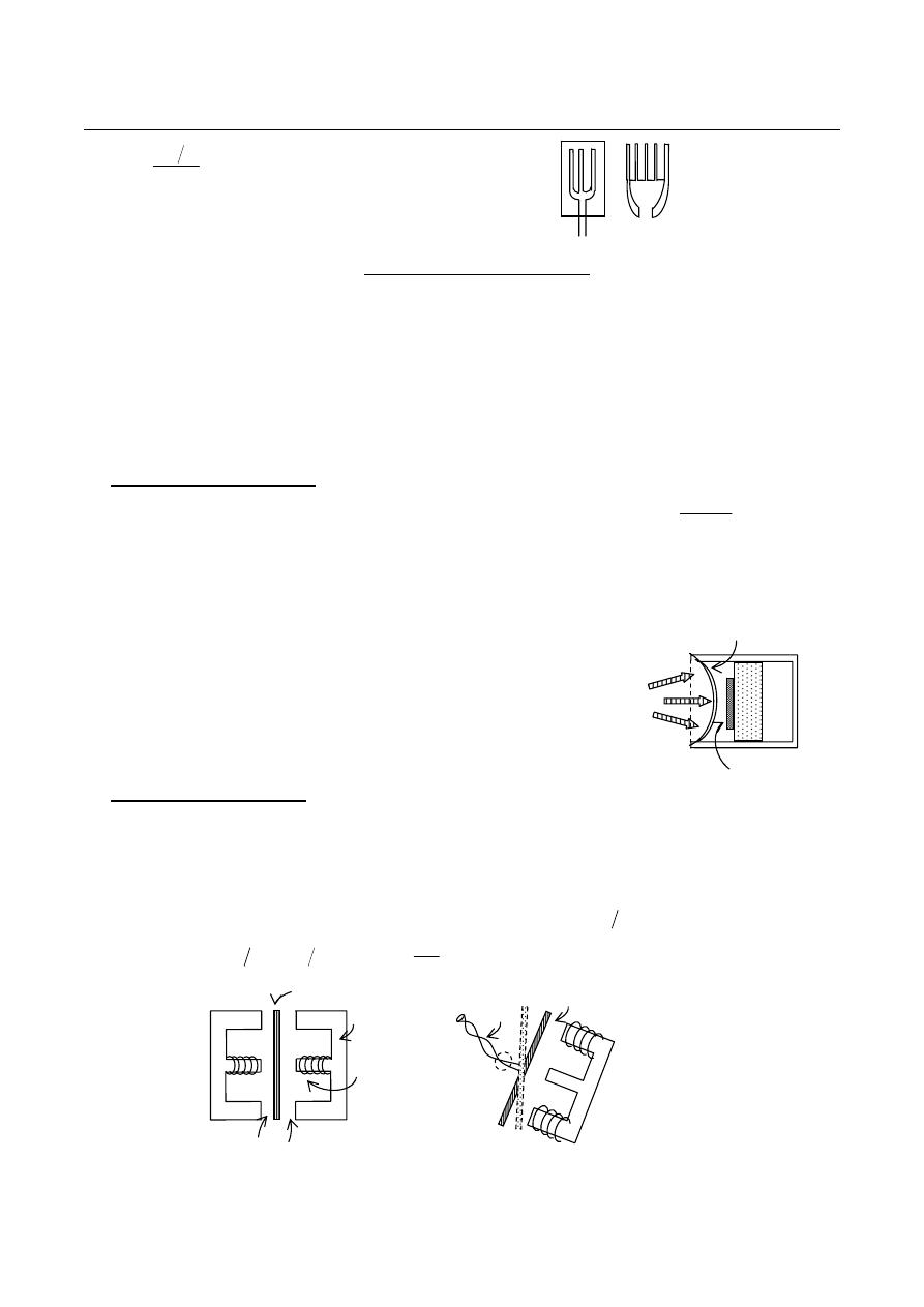
Variable Resistors:
The variable resistance usually have three leads, two fixed and one movable. If the contacts
are made to only
two leads of the resistor (stationary lead and moving lead), the variable
resistance is being employed as
a rheostat which limit the current flowing in circuit branches.
If all
three contacts are used in a circuit, it is termed a potentiometer or pot and often used as
voltage dividers to control or vary voltage across a circuit branch.
Lo
a
d
Load
V
in
Z
2
A
B
C
D
Z
4
R
2
C
3
Y
3
R
3
C
1
R
1
R
4
Z
1
Tenth Lecture Oscilloscope
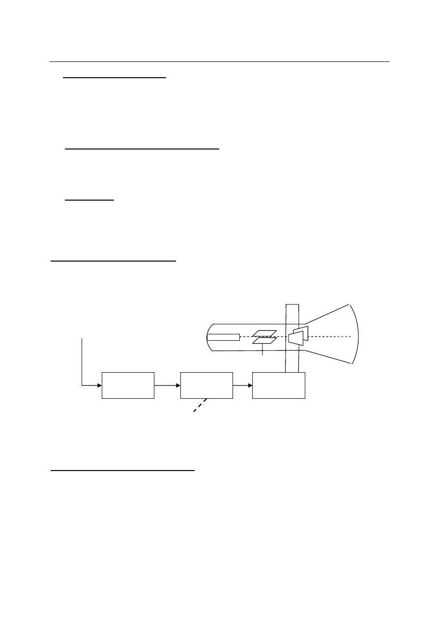
1
Oscilloscope
The cathode ray oscilloscope (CRO) is a device that allows the amplitude of electrical
signals, whether they are voltage, current; power, etc., to be displayed primarily as a function of
time. The oscilloscope depends on the movement of an electron beam, which is then made visible
by allowing the beam to impinge on a phosphor surface, which produces a visible spot
Oscilloscope Block Diagram:
General oscilloscope consists of the following parts:
1. Cathode ray tube (CRT)
2. Vertical deflection stage
3. Horizontal deflection stage
4. Power supply
The Cathode Ray Tube (CRT):
Cathode ray tube is the heart of oscilloscope which generates the electron beam,
accelerates the beam to high velocity, deflects the beam to create the image, and contains the
phosphor screen where the electron beam eventually become visible. There are two standard type
of CRT electromagnetic and electrostatic. Each CRT contains:
a)
One or more electron guns.
b)
Electrostatic deflection plates.
c)
Phosphoresce screen.
Vertical
Amplifier
Delay
Line
H.V
supply
L.V
supply
Trigger
Circuit
Time Base
Generator
Horizontal
Amplifier
To CRT
To All
Circuits
Time/Div
Volt /Div
Electron Gun
H
H
V
V
Screen
CRT
Vin
General Purpose Oscilloscope
Tenth Lecture Oscilloscope
2
A gun consists of a heated cathode, control grid, and three anodes.
A
heated cathode emits electrons, which are accelerated to the first accelerating anode,
through a small hole in the control grid. The amount of cathode current, which governs the
intensity of the spot, can be controlled with the control grid. The preaccelerating anode is a
hollow cylinder that is at potential a few hundred volts more positive than the cathode so that the
electron beam will be accelerated in the electric field. A focusing anode is mounted just a head of
the preaccelerating anode and is also a cylinder. Following the focusing anode is the accelerating
anode, which gives the electron beam its last addition of energy before its journey to the
deflecting plates. The focusing and accelerating anodes form an electrostatic lens, which bring
the electron beam into spot focus on the screen. Three controls are associated with the operating
voltages of the CRT; intensity, focus, and astigmatism
1-
The intensity control varies the potential between the cathode and the control grid
and simply adjusts the beam current in the tube.
2-
The focus control adjusts the focal length of the electrostatic lens.
3-
The astigmatism control adjusts the potential between the deflection plates and
the first accelerating electrode and is used to produce a round spot.
The electrostatic deflection system consists of two sets of plates for each electron gun. The
vertical plates move the beam up and down, while horizontal plates move it right and left. The
two sets of plates are physically separated to prevent interaction of the field. The position of the
spot at any instant is a resultant of potentials on the two set of plates at that instant.
The
viewing
screen is created by phosphor coating inside front of the tube. When
electron beam strikes the screen of CRT with considerable energy, the phosphor absorbs the
kinetic energy of bombarding electrons and reemits energy at a lower frequency range in visible
spectrum. Thus a spot of light is produced in outside front of the screen. In addition to light, heat
as well as secondary electrons of low energy is generating. Aquadag coating of graphite material
is cover the inside surface of CRT nearly up the screen to remove these secondary electrons.
The property of some crystalline materials such as phosphor or zinc oxide to emit light when
stimulates by radiation is called fluorescence.
Phosphorescence refers to the property of material to continue light emission even after the
source of excitation is cut off.
Persistence is the length of time that the intensity of spot is taken to decrease to 10% of its
original brightness.
Finally, the working parts of a CRT are enclosed in a high vacuum glass envelope to
permit the electron beam moves freely from one end to other with out collision.
cathode
gride
Preaccelerating
anode
Accelerating
anode
heater
Focusing
anode
Intensity
control
focusing
control
Astigmatism
control
Electron
beam
-
1500V
+300V
+ +
-
Tenth Lecture Oscilloscope
3
Graticules is a set of horizontal and vertical lines permanently scribed on CRT face to allow
easily measured the waveform values.
Electrostatic Deflection Equations:
Vin where Vin : input voltage to channel A or B of CRO
⇓
Av
Vin
Ed
.
=
Ed: deflection voltage (potential)
⇓
0
=
= Ez
Ex
Єy
d
Ed
−
=
…… (1) Єy: electrical field in Y direction
⇓ Єx= Єz=0
e
fy
−
=
.Єy Fy: force generate by electrical field effect
⇓ e: electron charge (1.6x10
-19
C)
0
=
= fz
fx
e
m
fy
ay
=
ay: acceleration in Y direction ,
0
=
= az
ax
⇓ m
e
: electron mass (9.1x10
-31
Kg)
t
cons
Vox
Vx
tan
=
=
0
=
Vz
ayt
Voy
Vy
+
=
Since
0
=
Voy
Vy: velocity in Y direction at any time
e
e
m
e
t
m
fy
ayt
Vy
−
=
=
=
Єy t
Voy: initial velocity in Y direction
⇓
2
2
1
ayt
Voy
Yo
Y
+
+
=
Since
0
=
Yo
0
=
Voy
Y: distance in Y direction
L
D
l
Ed
Ea
d
θ
Av
Vin
X
fy
Єy
e
e
P
l/2
l/2
y
(0,0)
Electron
gun
Screen
+
-
Vox
e
e
Y
X
Z
-X
-Y
Tenth Lecture Oscilloscope
4
e
m
e
ayt
Y
2
1
2
1
2
−
=
=
Єy
2
t Yo: initial distance in Y direction
e
m
e
Y
2
1
−
=
Єy
2
t …………. (2) Relation of Y with time
axt
Vox
Vx
+
=
Since
0
=
ax
Vox
Vx
=
Vx: velocity in X direction
⇓
2
2
1
axt
Voxt
Xo
X
+
+
=
Since
0
=
Xo
0
2
1
2
=
axt
Voxt
X
=
…….. (3) Relation of X with time
Vox
X
t
=
………… (4)
Substitute equ. (4) into equ.(2) give
e
m
e
Y
2
1
−
=
Єy
2
2
Vox
X
…….. (5) The parabolic equation of electron beam
eEa
mVox
=
2
2
1
where (Ea) is the acceleration voltage (potential)
m
eEa
Vox
2
=
………….. (6)
By substituting equs.(6) & (1) into equ.(5) we get
2
.
4
1
X
Ea
Ed
d
Y
⎟
⎠
⎞
⎜
⎝
⎛
=
…..…. (7)
⇐ Relation of Y with X
When the electrons leaves the region of deflecting plates, the deflecting force no longer exist, and
the electrons travels in a straight line toward point P. The slope of parabolic curve at distance
(x=l)
is:
2
tan
mVox
el
dx
dy
−
=
=
θ
Єy
Or
l
Ea
Ed
d
⎟
⎠
⎞
⎜
⎝
⎛
=
2
1
tan
θ
…….. (8)
The deflection on the screen (D) is
θ
tan
L
D
=
……….…… (9)
Substitute equ.(9) into (8) give
dEa
lLEd
D
2
=
…….…….. (10)
♣ The deflection sensitivity (S) of CRT is:
Ed
D
S
=
……………. (11)
L
D
x
y =
♣ The deflection factor (G) of CRT is:
lL
dEa
D
Ed
S
G
2
1
=
=
=
…… (12)
y
x
D
L
θ
By similarity
Eleventh Lecture Oscilloscope (2)
1
Post Deflection Acceleration:
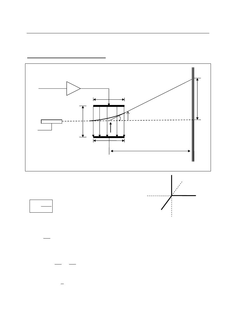
The amount of light given off by the phosphor depends on the amount of energy that is
transferred to the phosphor by the electron beam. For fast oscilloscope (of high frequency
response greater than 100MHz), the velocity of electron beam must be great to respond to fast
occurring events; otherwise, the light output will be drop off. This is done by increasing the
acceleration potential but it will be difficult to deflected the fast electron beam by the deflection
plates because this would required a higher deflection voltage and a higher deflection current to
charge the capacitance of the plates.
Modern CRTs use a two step acceleration to eliminate this problem. First, the electron
beam is accelerated to a relatively low velocity through a potential of a few thousand volts. The
beam is then deflected and after deflection is further accelerated to the desired final velocity.
The deflection sensitivity of the CRT depends on the acceleration voltage before the deflection
plates, which is usually regulated and does not depends on the post acceleration voltage after the
deflection plates.
Vertical deflection system:
The vertical deflection system provides an amplified signal of the proper level to derive
the vertical deflection plates with out introducing any appreciable distortion into the system. This
system is consists of the following elements:
1-
Input coupling selector.
2-
Input attenuator.
3-
Preamplifier.
4-
Main vertical amplifier.
5-
Delay line.
Electron Gun
H
H
V
V
Screen
CRT
+25 KV
Post deflection
Accelerating voltage
Coupling
Selector
Delay Line
Vin
to Trigger
Circuit
Screen
Vertical Deflection System
Input
Attenuator
Vertical
Amplifier
Vertical
Amplifier
a.c
d.c
GND
Eleventh Lecture Oscilloscope (2)
2
1- Input Coupling Selector:
Its purpose is to allow the oscilloscope more flexibility in the display of certain types of
signals. For example, an input signal may be a d.c signal, an a.c signal, or a.c component
superimposed on a d.c component. There are three positions switch in the coupling selector
(d.c, a.c, and GND). If an a.c position is chosen, the capacitor appears as an open circuit to
the d.c components and hence block them from entering. While the GND position ground the
internal circuitry of the amplifier to remove any stored charge and recenter the electron beam.
2- 4- Input Attenuators And Amplifiers:
The combine operation of the attenuator, preamplifier and main amplifier together make up
the amplifying portion of the system.
The function of the attenuator is to reduce the amplitude of the input signal by a selected
factor and verse varies amplifier function.
5- Delay Line:
Since part of the input signal is picked off and fed to the horizontal deflection system to
initiate a sweep waveform that is synchronized with the leading edge of the input signal. So the
purpose of delay is to delay the vertical amplified signal from reaching the vertical plates until
the horizontal signal reach the horizontal plates to begin together at the same time on CRT
screen.
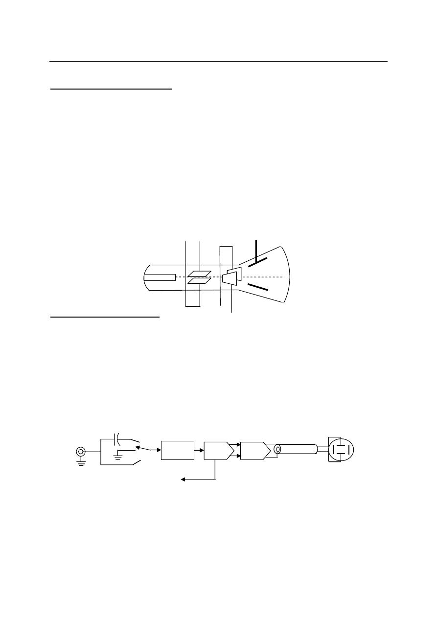
Horizontal Deflection System:
The horizontal deflection system of OSC consist of :
1- Trigger circuit.
2- Time base generator.
3- Horizontal amplifier.
Trigger and Time Base Generator:
The most common application of an oscilloscope is the display of voltage variation versus
time. To generate this type of display a saw tooth waveform is applied to horizontal plates. The
electron beam being bent towards the more positive plate and deflected the luminous spot from
left to right of the screen at constant velocity whilst the return or fly back is at a speed in excess
of the maximum writing speed and hence invisible. The saw tooth or time base signal must be
repetitively applied to the horizontal plates so that; the beam can retrace the same path rapidly
enough to make the moving spot of light appear to be a solid line.
Trigger
Circuit
Time Base
Generator
Horizontal
Amplifier
Time/Div
Electron Gun
H
H
V
V
Screen
CRT
Horizontal Deflection System
From Vertical
Amplifier

Eleventh Lecture Oscilloscope (2)
3
To synchronous the time base signal applied to (X-plates) with input voltage to be
measured which applied to vertical or (Y-plates) a triggering circuit is used. This circuit is
sensitive to the level of voltage applied to it, so that when a predetermined level of voltage is
reached a pulse is passed from the trigger circuit to initiate one sweep of the time base. In a
practical oscilloscope the time base will be adjustable from the front panel control of scope.
Horizontal Amplifier:
The horizontal amplifier is used to amplify the sweep waveform to the required level of
horizontal plates operation.

Twelveth Lecture Transducers
1
Transducers
The input quantity for most instrumentation system is nonelectrical. In order to use electrical
methods and techniques for measurement, manipulation, or control the nonelectrical quantity is
converted into an electrical signal by a device called electrical transducer.
Transducers are broadly defined as devices that convert energy or information from one form
to another. This energy may be electrical, mechanical, chemical, optical (radiant), or thermal. Such as,
for example, mechanical force or displacement, liner and angular velocity heat, light intensity,
humidity, temperature variation, sound time, pressure, all are converted into electrical energy by
means of electrical transducers.
Transducers may be classified according to their application, method of energy conversion,
nature of output signal, and so on.
1- Primary and Secondary Transducers:
Transducers, on the basis of methods of applications, may be classified into primary and
secondary transducers. Transducer that converts energy from any form to electrical form is called
primary transducer, such as a photovoltaic cell, while transducer that converts energy from any
form to another form but not electrical energy or signal is called secondary transducer, such as
displacement transducer (which converts force or pressure to displacement).
2- Active and Passive Transducers:
Transducers, on the basis of methods of energy conversion used, may be classified into active
and passive transducers.
Active (self generating) transducers develop their output in the form of electrical voltage or current
without any source of electrical excitation, such as thermocouples, tacho generator.
While, if the transducer is capable of producing an output signal only when it is in connection
with electrical power source is called passive transducers, such as a potentiometer, thermistor (thermal
resistance). Passive transducer producing a variation in some electrical parameter, such as a resistance,
capacitance, inductance and so on, which can be measured as voltage or current variation in the circuit.
3- Analog and Digital Transducers:
Transducers, on the basis of nature of output signal, may be classified into analog and digital
transducer.
Analog transducer converts input signal into output signal, which is a continuous function of
time, while digital transducer converts input signal into output signal in a discrete forms.
Strain Gauges
The strain gauge is an example of a primary passive analog transducer that converts force or
small displacement into a change of resistance. Since many other quantities such as torque,
pressure, weight, and tension also involve force or displacement effects, they can also be measured
by strain gauges.
Strain gauges are so named because when they undergo a strain (defined to be a fractional change
in linear dimension tension or compression caused by an applied force); they also undergo a
change in electrical resistance. The strain takes the form of a lengthening of the special wire from
which the gauge is constructed. The change in resistance is proportional to the applied strain and is
measured with a specially adopted Wheatstone bridge.
The gauge factor (k) is given by:
l
l
R
R
k
Δ
Δ
=
, where
A
l
R
δ
=
and
(
)
2
4 d
l
R
Π
=
δ
since the strain
( )
l
l
Δ
=
σ
thus
Twelveth Lecture Transducers
2
σ
R
R
k
Δ
=
and
σ
kR
R
=
Δ
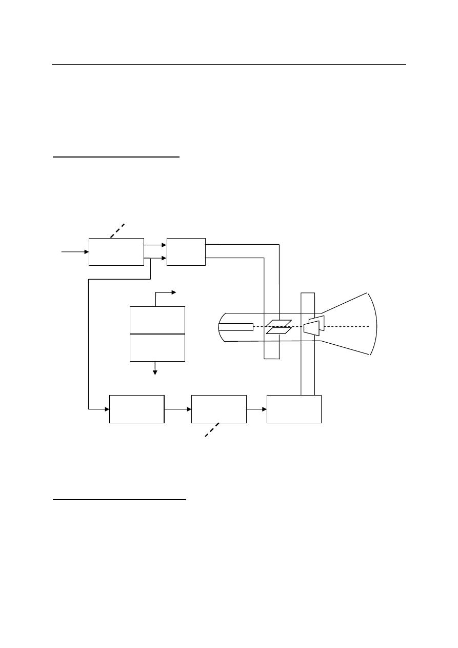
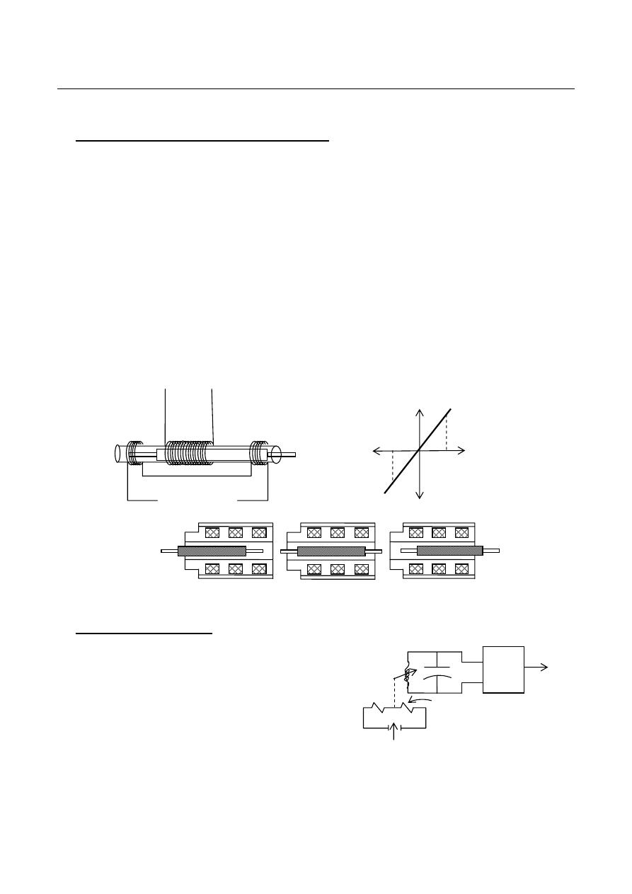
Displacement transducers
The mechanical elements that are used to convert the applied force into a displacement are
called force summing devices. The force summing members generally used the following:
a) Diaphragm, flat or corrugated b) Bellows c) Bourdon tube, circular or twisted
d) Straight tube e) Mass cantilever, single or double suspension f) Pivot torque
The displacement created by the action of the force summing device is converted into a change of
some electrical parameter and measured by one of the following electrical principle:
1) Capacitive 2) Inductive 3) Differential transformer 4) Photoelectrical
5) Potentiometer 6) Ionization 7) Oscillation 8) Piezoelectric 9) Velocity
1- Capacitive Transducer:
The capacitance of a parallel plate capacitor is given by
d
A
C
r
o
ε
ε
=
, where
12
10
85
.
8
−
×
=
o
ε
F/m and
=
r
ε
relative dielectric constant
A force applied to a diaphragm that function as one plate of a simple capacitor, change the distance
between the diaphragm and static plate.
The resulting change in capacitance could be measured with
an ac bridge, but it is usually measured with an oscillator circuit.
The transducer as a part of oscillator circuit will causes
a change in oscillator frequency which proportional
to the applied force.
2- Inductive Transducer:
In the inductive transducer the measurement of force is accomplished by the change in the
inductance ratio of a pair of coils or by the change of inductance in a single coil. The ferromagnetic
armature is displaced by the force being measured, varying the reluctance of the magnetic circuit. The
air gap is varied by a change in position of the armature; the resulting change in inductance is a
measure of applied force.
force→displacement→air gap change→permaebility(μ) →
A
l
μ
=
ℜ
→
→
ℜ
=
ℜ
=
Φ
NI
mmf
→
i
N
L
∂
Φ
∂
=
Deflected
diaphragm
Static plate
Pressure
Diaphragm
or mass
air gaps
E-core
Coil
winding
Double coil
Bourdon
tube
armature
Single coil
Twelveth Lecture Transducers
3
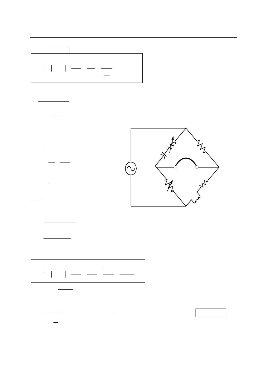
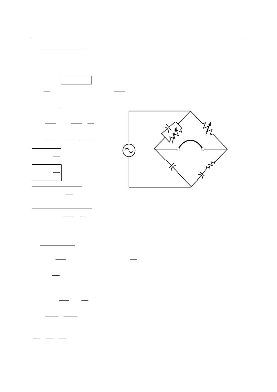
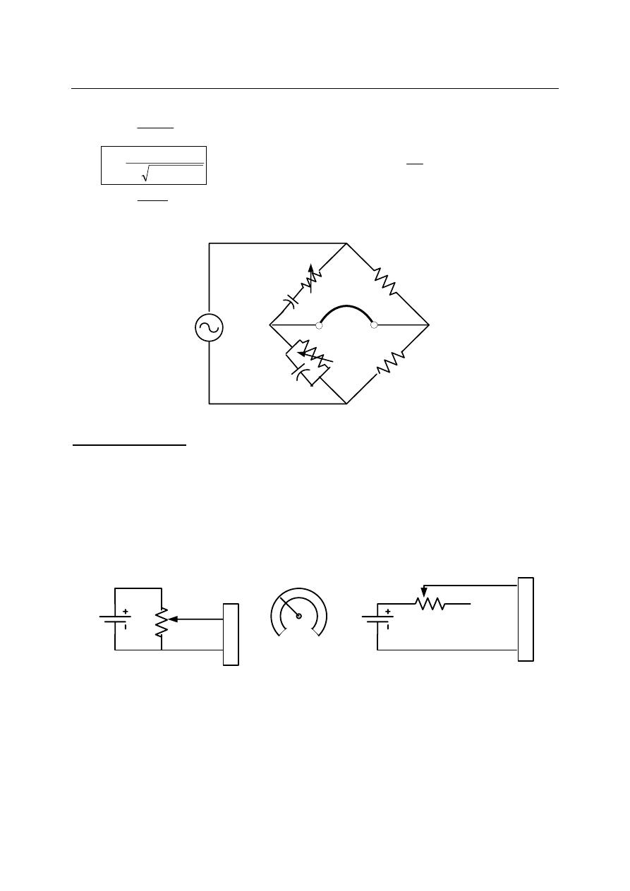
3- Linear Variable Differential Transformer:
It is produces an electrical signal that is linearly proportional to mechanical displacement. The
displacements detectable by LVDTs are relatively large compared to those detectable by strain gauges.
LVDT consists of a single primary winding and two secondary windings which are placed on
either side of the primary. The secondary windings have an equal number of turns but they are
connected in series opposition so that the emf induced in the coil oppose each other. The position of the
moveable core determines the flux linkage between the ac excited primary winding and each of the two
secondary winding.
a)
With the core in the centre, or reference position, the induced emfs in the secondaries are equal,
and since they oppose each other, the output voltage will be zero.
b)
When the core is forced to move to the left, more flux links the left hand coil than the right hand
coil, the induced emf of the left coil is therefore larger than the induced emf of the right coil. The
magnitude of the output voltage is than equal to the difference between the two secondary voltages,
and it is in phase with the voltage of the left hand coil.
c)
Similarly, when the core is force to move to the right, more flux links the right hand coil than the
left hand coil and the result output is now in phase with the emf of the right hand coil, while its
magnitude again equals the difference between the two induced emfs.
4- Oscillator Transducer:
This class of oscillator uses the force summing member to change
the capacitance or inductance in an (LC) oscillator circuit, which
change the frequency of the circuit in proportional to the applied
force.
Oscillator
C
L
Force summing
member
Pressure
FM o/p
Mechanical
linkage
Core at 0
Core at A
Core at B
Primary
wind
C
t A
Secondary
winding (1)
Secondary
winding (2)
Vo=V1-V2
Ac supply
voltage
B
A
0
Vo
+
_
Phase of
coil (2)
Phase of
coil (1)
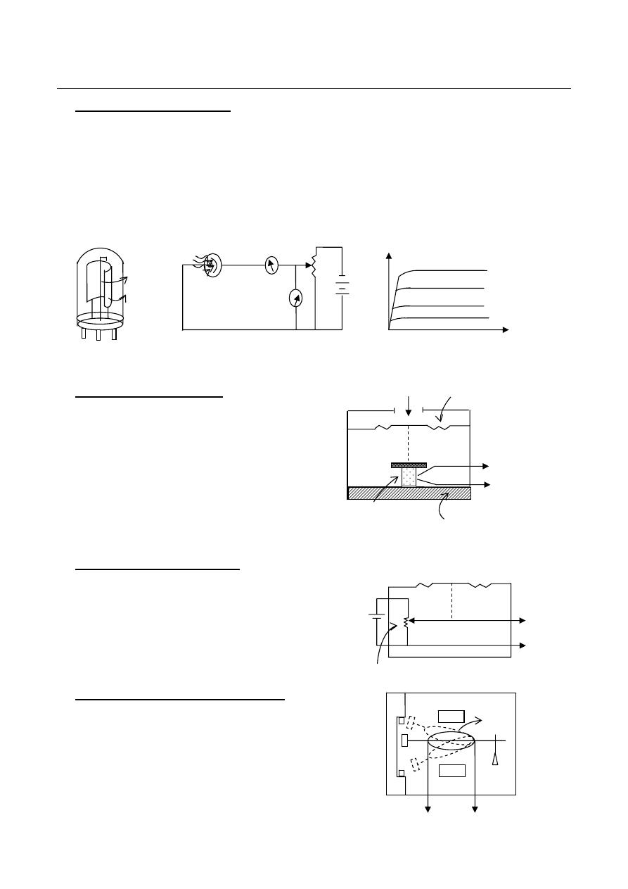
Twelveth Lecture Transducers
4
Vo
Force summing member
pressure
crystal
base
Vo
Force summing member
Potentiometer
Vo
N
S
Moving coil
5- Photoelectric Transducer:
The photoelectric transducer makes use of the properties of photo emissive cell or phototube. The
phototube is a radiant energy device that controls its electron emission when exposed to incident light.
The large semicircular element is the photosensitive cathode and the thin wire down the centre of the
tube is the anode. Both elements are place in a high vacuum glass envelope. When a constant voltage is
applied between cathode and anode, the current is directly proportional to the amount of light falling on
the cathode. The output current is extremely small in (μA) and for a voltage approximately above 20V,
the output current is nearly independent of the applied anode voltage but depends entirely on the
amount of the incident light.
6- Piezoelectric transducer:
A symmetrical crystalline material, such as quartz,
Rochelle salt, and barium titanate, produce an emf
when they are placed under stress. This property is used
in piezoelectric transducer.
When a crystal is placed between a solid base and the
force summing member, an externally applied force,
entering the transducer through its pressure port,
applies pressure to the top of a crystal; this will produce
a small emf proportional to the applied force or pressure.
7- Potentiometric Transducer:
A Potentiometric transducer is an electromechanical device
containing a resistance element that is contacted by a
movable slider. Motion of the slider results in a resistance
change that may be linear, logarithmic, exponential, and so
on, depending on the manner in which the resistance wire is
wound.
8- Velocity Transducer (Tachometer):
The velocity transducer essentially consists of a moving coil
suspended in the magnetic field of a permanent magnet. A
voltage is generated by the motion of the coil in the field which
is proportional to the velocity of the moving coil. It is used for
velocity measurement.
Anode
cathode
Ia
(μA)
Va
(volt)
0.8
0.6
0.4
0.2
Light flux(lumen)
20 40 60 100 120
10
5
15
20
μA
volt
light
phototube
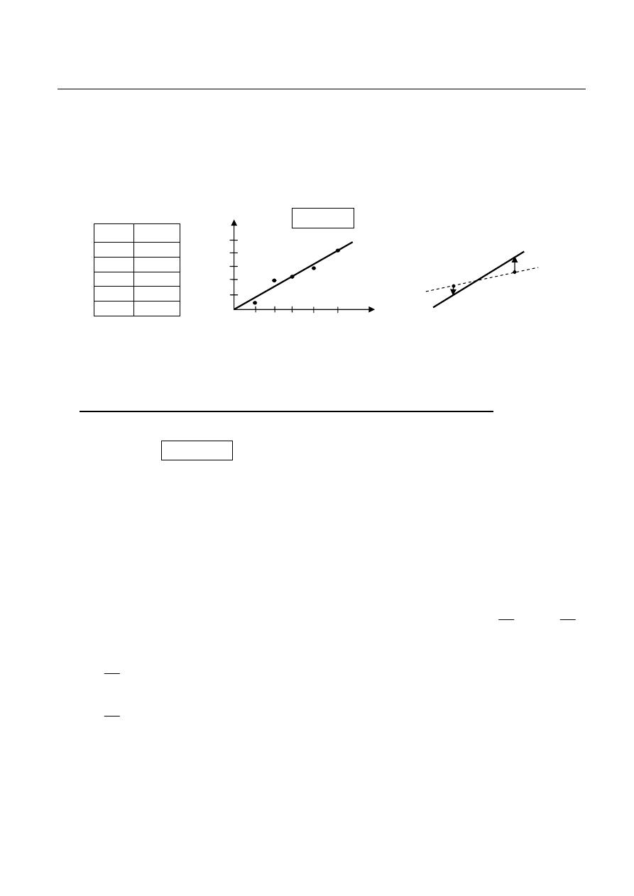
Thirteenth Lecture Curve Fitting and Approximation by LSA
1
Curve Fitting and Approximation by
Least Square Approximations Method
Suppose we wish to fit a curve to an approximate set of data such as from the determination of
the effects of temperature on resistance, we want to suitably determine the constants (a) and (b) in the
equation relating resistance R and temperature T, we shall assume that the error of reading the
temperature is negligible, so that all the errors are in the resistance measurements, and use vertical
distance.
We want to minimize the deviations of the points from the line (errors). The deviations are measured by
the distances from the point to the line. The deviation could be minimizing by making their sum
minimum, but this is not an adequate criterion.
1- Fitting linear curves by Least Square Approximations (LSA) method:
Let (Yi) represent an experimental value, and let (y
i
) represent the theoretical value which get by
this equation
b
aX
y
i
i
+
=
where (X
i
) is a particular value of the variable assumed free from
error. We wish to determine the best values for (a) and (b), so that (y
i
) predict the function values that
correspond to x-values.
Since error= measured- theoretical thus
i
i
i
y
Y
e
−
=
Least squares method criterion requires that the sum of errors in the reading (S) must be minimized, so
min
2
2
4
2
3
2
2
2
1
=
+
⋅
⋅
⋅
+
+
+
+
=
N
e
e
e
e
e
S
where N is the number of the measured points
(
)
(
)
∑
∑
∑
=
=
=
=
−
−
=
−
=
=
N
i
N
i
N
i
i
i
i
i
i
b
aX
Y
y
Y
e
S
1
1
1
2
2
2
min which reach the minimum by proper
choice of parameters (a) and (b). When S be a minimum, the two partial derivatives
⎟
⎠
⎞
⎜
⎝
⎛
∂
∂
a
S and
⎟
⎠
⎞
⎜
⎝
⎛
∂
∂
b
S
will be zero. Thus
(
)(
)
0
2
1
=
−
−
−
=
⎟
⎠
⎞
⎜
⎝
⎛
∂
∂
∑
=
N
i
i
i
i
X
b
aX
Y
a
S
………… (1)
(
)( )
0
1
2
1
=
−
−
−
=
⎟
⎠
⎞
⎜
⎝
⎛
∂
∂
∑
=
N
i
i
i
b
aX
Y
b
S
…………... (2)
Dividing each of these equations by (-2) and expanding the summation, we get
(
)
∑
∑
∑
∑
=
=
=
=
=
−
−
=
−
−
N
i
N
i
i
N
i
i
i
i
N
i
i
i
i
i
X
b
X
a
X
Y
bX
aX
X
Y
1
1
1
2
1
2
0
T(C
o
) R(Ω)
20.5 765
32.7 826
51.0 873
73.2 942
95.7 1032
Xi
R (Ω)
T (C
o
)
R=aT+b
Yi
+
e
-e
Thirteenth Lecture Curve Fitting and Approximation by LSA
2
(
)
∑
∑
∑
∑
=
=
=
=
=
−
−
=
−
−
N
i
N
i
N
i
N
i
i
i
i
i
b
X
a
Y
b
aX
Y
1
1
1
1
0 note that:
∑
=
=
N
i
Nb
b
1
The normalized equations
∑
∑
∑
=
=
=
=
+
N
i
N
i
N
i
i
i
i
i
X
Y
X
b
X
a
1
1
1
2
………. (1)
∑
∑
=
=
=
+
N
i
i
N
i
i
Y
bN
X
a
1
1
………………. (2)
Solving these equations simultaneously gives the values for the slope and intercept (a) and (b).
For the data of previous example, we find that
N=5 ∑T
i
= ∑X
i
=273.1 ∑T
i
2
=18607.27 ∑R
i
=∑Y
i
=4438 ∑T
i
R
i
=∑Y
i
X
i
=2549325
The normalized equations are then
18607.27 a + 273.1 b = 254932.5 ……. (1)
273.1 a + 5 b = 4438 …………………. (2)
By solving these equations we obtain a=3.395 , b=702.17
And hence the equation R=aT+b will be R= 3.39T + 702.17
To find R at T=70 is R(70)=3.39x70+702.17=939.3 Ω
The measured and theoretical values are then
T(C
o
)
20.5 32.7 51.0 73.2 95.7
R
measured
765 826 873 942 1032
R
theoretical
772 813 875 950 1026
Exercise:
Find the theoretical values for linear equation (y) from the given data
Xi 6 8 10 12 14 16 18 20 22 24
Yi 3.8 3.7 4 3.9 4.3 4.2 4.2 4.4 4.5 4.5
yi
a=0.0445 b=3.48
2- Fitting nonlinear curves by Least Square Approximations method:
In many cases, of course, data from experimental test are not linear, so we need to fit other function
than a first degree polynomial, popular forms that are tried are the exponential forms such as
b
ax
y
=
or
bX
ae
y
=
The exponential forms are usually linearized by taking logarithms before determining the
parameters, so for the first equ.
X
b
a
y
ln
ln
ln
+
=
, then let ln y=z , ln a= A, ln X=w
Thus z=A+bw is a linear equation

Thirteenth Lecture Curve Fitting and Approximation by LSA
3
Solving this equation to find the values of (A) and (b) then find the value of (a)
i
i
i
z
Z
e
−
=
(
)
(
)
∑
∑
∑
=
=
=
=
−
−
=
−
=
=
N
i
N
i
N
i
i
i
i
i
i
bw
A
Z
z
Z
e
S
1
1
1
2
2
2
min
(
)( )
0
1
2
1
=
−
−
−
=
⎟
⎠
⎞
⎜
⎝
⎛
∂
∂
∑
=
N
i
i
i
bw
A
Z
A
S
…….. (1)
(
)(
)
0
2
1
=
−
−
−
=
⎟
⎠
⎞
⎜
⎝
⎛
∂
∂
∑
=
N
i
i
i
i
w
bw
A
Z
b
S
.…. (2)
Dividing each of these equations by (-2) and expanding the summation, we get
(
)
∑
∑
∑
∑
=
=
=
=
=
−
−
=
−
−
N
i
N
i
N
i
i
N
i
i
i
i
w
b
A
Z
bw
A
Z
1
1
1
1
0 ………. (1)
(
)
∑
∑
∑
∑
=
=
=
=
=
−
−
=
−
−
N
i
N
i
i
N
i
i
i
i
N
i
i
i
i
i
w
b
w
A
w
Z
bw
Aw
w
Z
1
1
2
1
1
2
0 …………… (2)
The normalized equations
∑
∑
∑
=
=
=
=
+
N
i
N
i
N
i
i
i
i
i
w
Z
w
A
w
b
1
1
1
2
………. (1)
∑
∑
=
=
=
+
N
i
i
N
i
i
Z
AN
w
b
1
1
………………. (2)
Solving these equations simultaneously gives the values of (A) and( b) and by taking the inverse ln of
(A) we can get the value of (a).
Home work:
Derive the normalized equations for
bX
ae
y
=
Example:
The
results
obtained for some experimental measurement is:
Xi
1 2 3 4
Yi 7 11 17 27
The variable is varied according the function
bX
ae
y
=
fit the curve by LSA method.
Sol:
Taking the logarithms for above equ.
ln y= ln a + bx ln e , since ln e =1 , so ln y= ln a + bx , let ln y=z , ln a =A thus
z=A+bx , by deriving this equation the normalized equations will be
Thirteenth Lecture Curve Fitting and Approximation by LSA
4
∑
∑
∑
=
=
=
=
+
N
i
N
i
N
i
i
i
i
i
x
Z
x
A
x
b
1
1
1
2
…………… (1)
∑
∑
=
=
=
+
N
i
i
N
i
i
Z
AN
x
b
1
1
………. (2)
N=4, ∑xi=10 , ∑xi
2
=30 , ∑Zi=10.471, ∑Zixi=28.42
30 b+ 10 A =28.42 …….. (1)
10 b + 4 A =10.471 ….. (2)
Solving these equs.
b
b
A
5
.
2
61775
.
2
4
10
471
.
10
−
=
−
=
[
]
42
.
28
5
.
2
61775
.
2
10
30
=
−
+
b
b
→→→→
42
.
28
25
1775
.
26
30
=
−
+
b
b
4485
.
0
=
b
4965
.
1
=
A
466
.
4
ln
1
=
=
−
A
a
, thus
x
z
448
.
0
4965
.
1
+
=
and
X
e
y
448
.
0
466
.
4
=
Xi 1
2
3
4
Yi 7
11 17 27
lnYi 1.946 2.397 2.833 3.295
yi 6.99 10.94
17.12
26.8