2
nd
Lec. M.Community Descriptive Statistics (Summarization of data)
Learning objectives
At the end of the lecture the student will be able to :
1. Calculate and interpret the following measures of central location:
-arithmetic mean
-median
-mode
-geometric mean
2. Choose and apply the appropriate measure of central location.
3. Calculate and interpret the following measures of dispersion:
- range
-interquartile range
-variance
-standard deviation
-coefficient of variation
4. Choose and apply the appropriate measure of dispersion
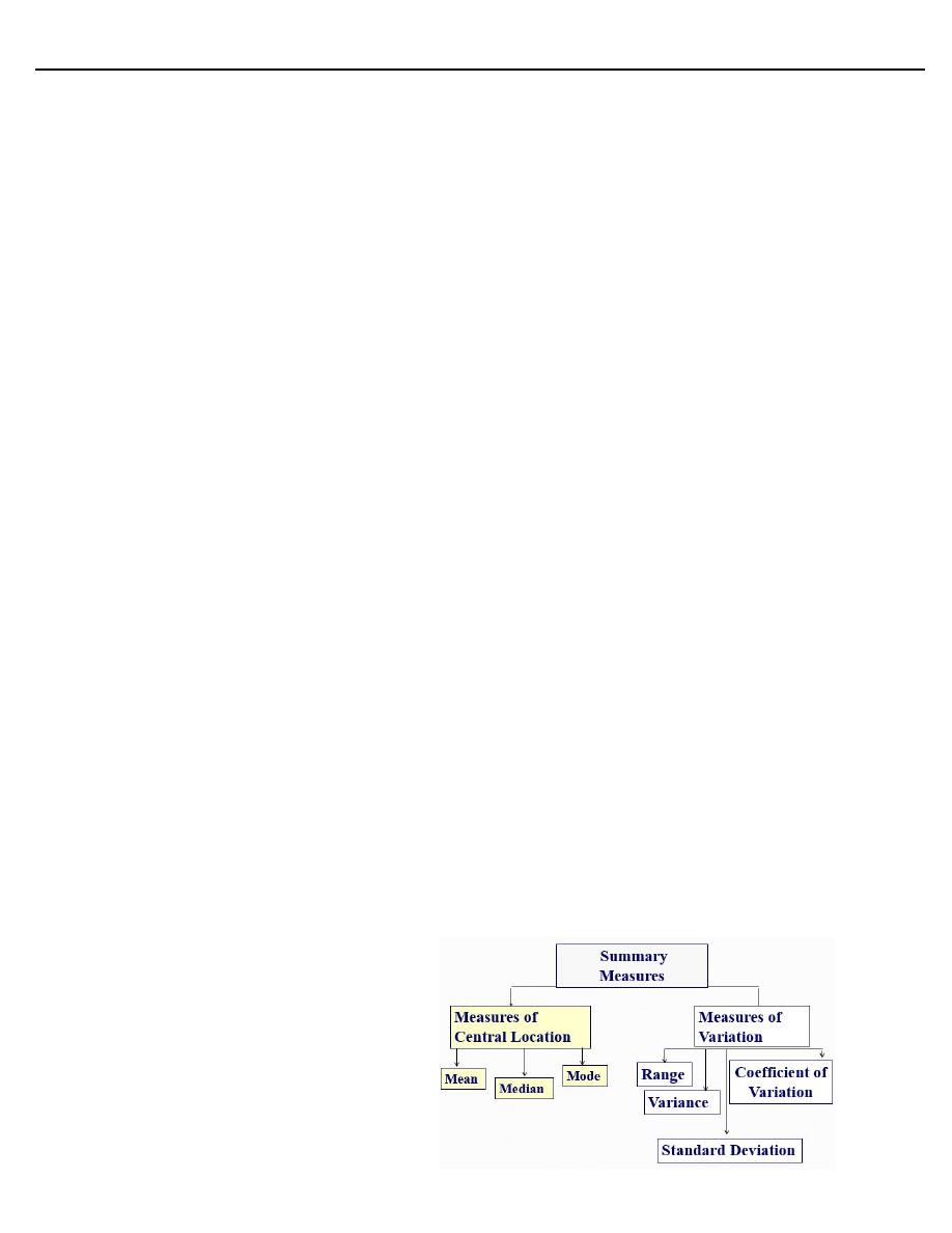
Summarization of Data (Measures of Central Location and Dispersion)
▪ Two types of summary measures are used when describing data ( distribution):
1. Measures of Central location
2. Measures Variability or spread
Important Summary Measures
Measures of Central Location
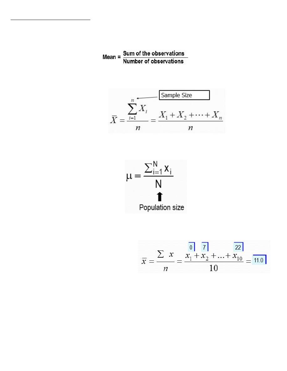
1. The mean (arithmetic mean):
The mean is the average of all the data values in a distribution
Mean (Arithmetic Mean)
Sample mean
Population mean
The Mean
Example : The reported time on the Internet
of 10 adults are 0, 7, 12, 5, 33, 14, 8, 0, 9, 22
hours. Find the mean time on the Internet.
Properties of the mean:
A. The most commonly used measure of central location
B. Uses every value (uses all observations)
C. Influenced by extreme values (high or low)
D. For each set of data there is only one mean.
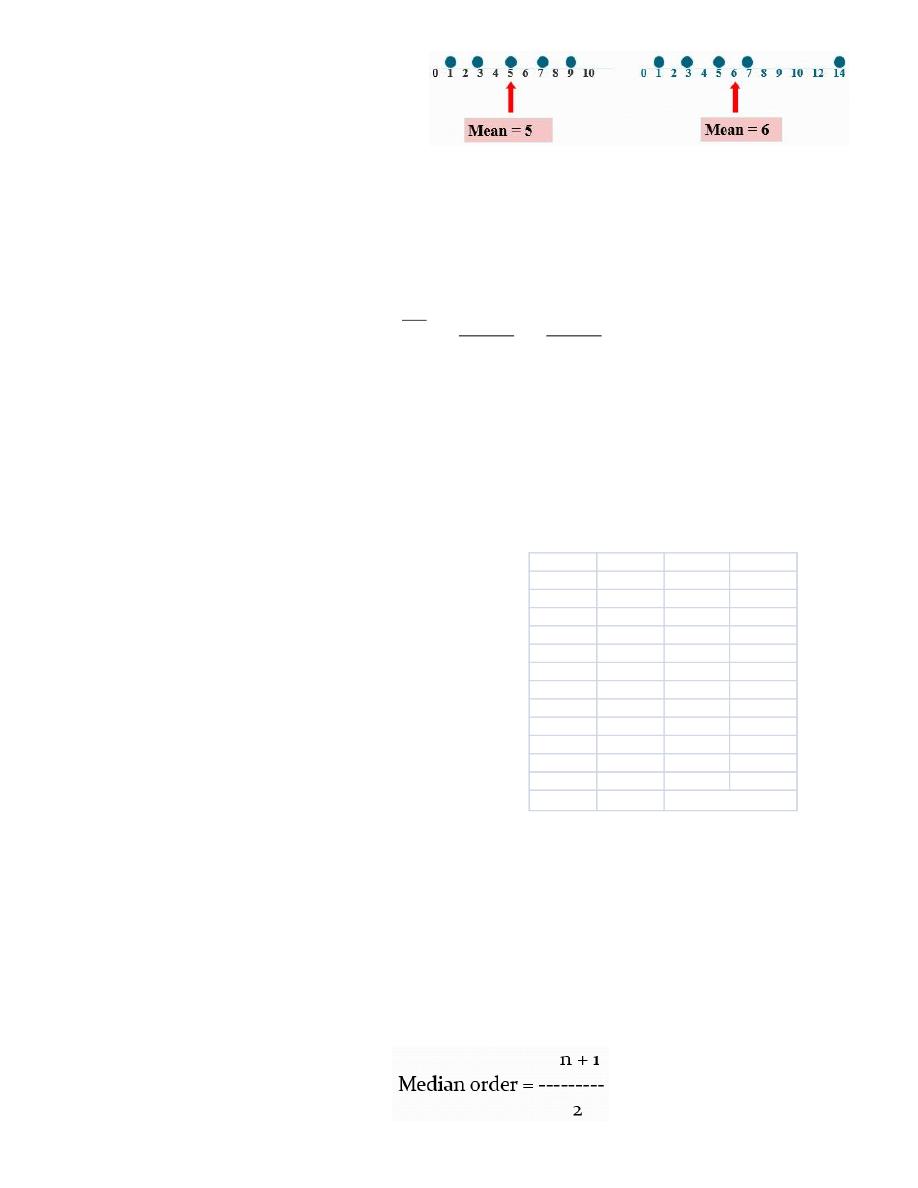
• Affected by extreme values (outliers)
The Mean of Grouped Data
➢ The mean of a sample of data organized in a frequency distribution is computed by the
following formula:
➢ Where:
• ΣXf, the X value is the class midpoint and the f value is the class frequency
• Σf is the sum of the frequencies
• n is the sample size
Example of mean calculation
Calculation of the mean weight of infants.
2. The Median
The Median is the “middle” value when the observations are arranged in ascending or descending
order.
Steps for finding the median
1. Arrange observations in ascending or descending order
2. Find the position of the median (order of the median):
n
Xf
f
Xf
X
=
=
freq f
mid point x
f x
3.6 -
9
3.7
33.3
3.8 -
25
3.9
97.5
4.0 -
42
4.1
172.2
4.2 -
61
4.3
262.3
4.4 -
77
4.5
346.5
4.6 -
86
4.7
404.2
4.8 -
67
4.9
328.3
5.0 -
26
5.1
132.6
5.2-
5
5.3
26.5
5.4 - 5.6
2
5.5
11.0
400
1814.4
Mean =
f x / f = 1981.6/400 = 4.95
fx/
∑
f
1814.4/400=4.536
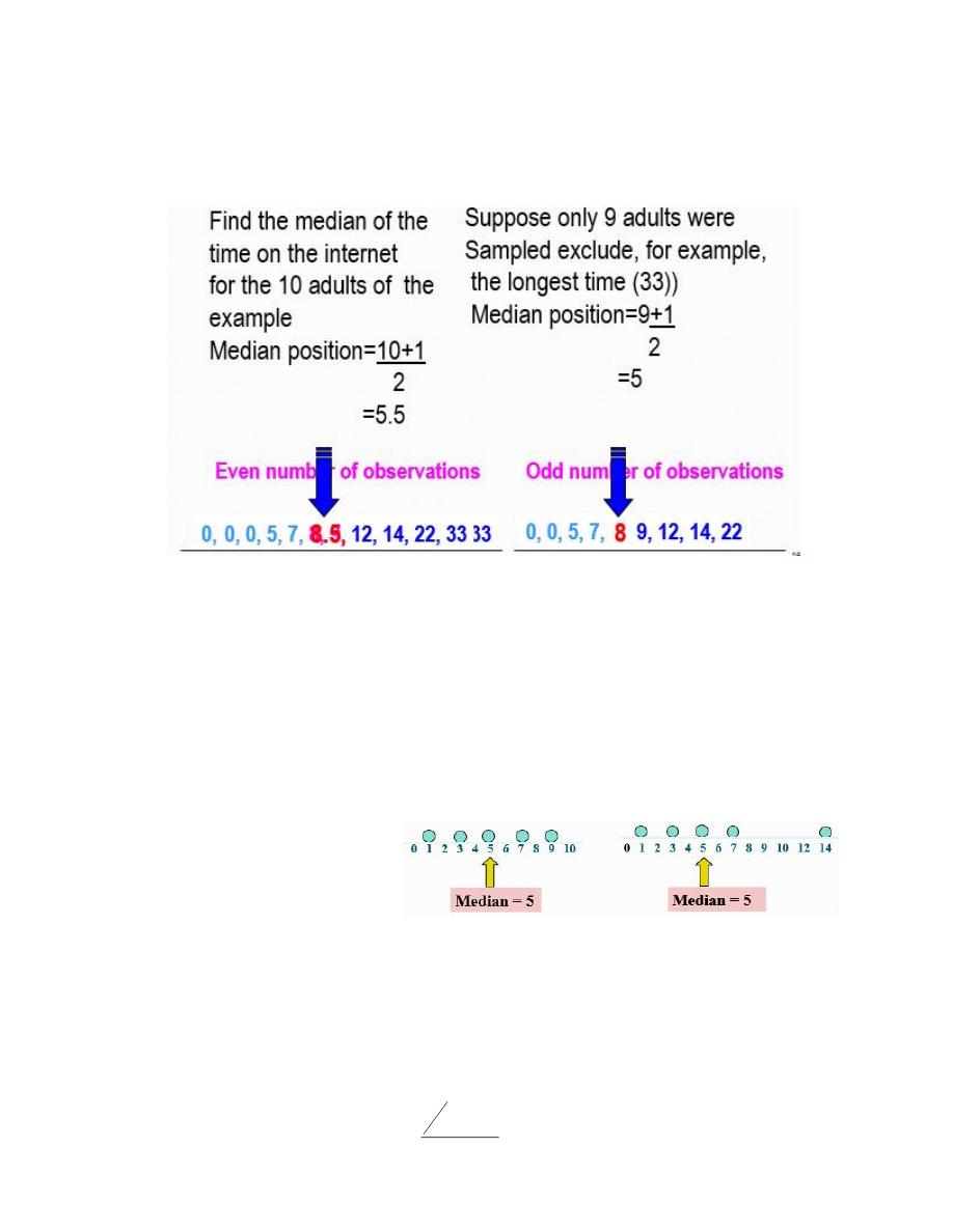
If n is odd, the median is the middle number
If n is even, the median is the average of the two middle numbers
Example
Properties of the median:
A. It divides the observations into two equal halves (50% of the observations above and 50%
below the median)
B. It is not affected by extreme values
C. For each set of data there is only one median.
Not affected by extreme values.
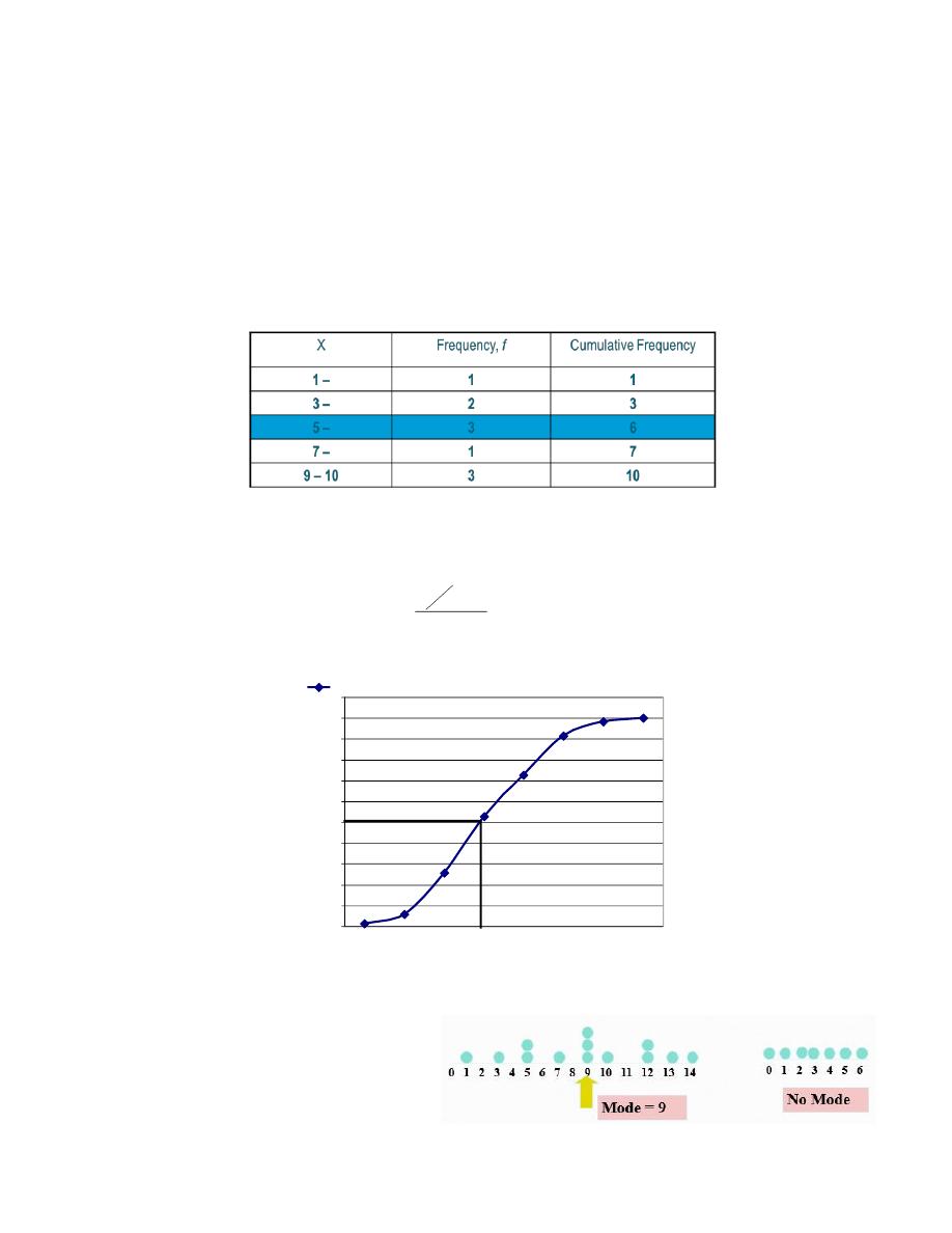
The Median of Grouped Data
➢ The median of a sample of data organized in a frequency distribution is computed by the
following formula:
w
f
CF
n
L
Median
.
2
−
+
=
➢ Where:
• L is the lower limit of the median class
• n is the sample size
• CF is the cumulative frequency preceding the median class
• f is the frequency of the median class
• w is the width of the class interval.
Example
The median class is 5 – 6, since it contains the 5th value (n+1/2=5.5).
From the table, L = 5, n = 10, f = 3, i = 2, & CF = 3.
Thus, the median
3. The Mode
➢ The mode is the most frequently
occurring value.
➢ It is the value that has the highest
frequency.
0%
10%
20%
30%
40%
50%
60%
70%
80%
90%
100%
110%
8.5
9.5
10.5
11.5
12.5
13.5
14.5
15.5
c.r.f.%
33
.
6
)
2
)(
3
3
2
10
(
5
=
−
+
=
Properties of the mode
➢ Not affected by extreme values
➢ Used for both quantitative and categorical data
➢ There may be no mode
➢ There may be one mode (unimodal), two modes (bimodal) , or three modes (trimodal) …….etc
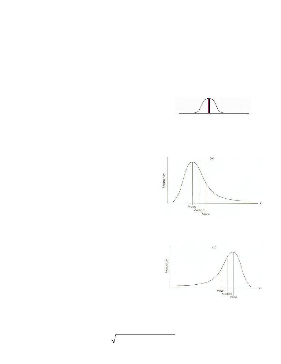
Relationship among Mean, Median, and Mode
If a distribution is symmetrical, the mean, median and
mode coincide
• If a distribution is non symmetrical, and skewed to the left or to the right, the three measures
differ.
Right Skewed Distribution
Positively skewed: Mean and Median are to the
right of the Mode
Mode < Median < Mean
Left Skewed Distribution
Negatively skewed: Mean and Median are to the
left of the Mode
Mean < Median < Mode
The Geometric Mean
Definition: The geometric mean (GM) of a set of n numbers is defined as the nth root of the
product of n numbers. The formula for the geometric mean is given by:
n
n
X
X
X
X
GM
)
)...(
)(
)(
(
3
2
1
=
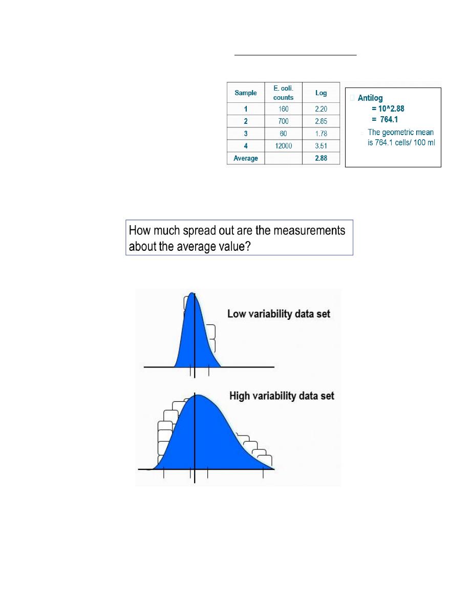
Geometric mean is also defined as the antilog of the mean of the logs x
i
The geometric mean
Take the logarithm of each score
Average the log values (mean of the logs)
Calculate the antilog
Measures of variation
Measures of central location fail to answer the the following question:
Observe two hypothetical data sets
n
X
X
X
anti
ean
Geometricm
n
log
...
log
log
log
2
1
+
+
+
=
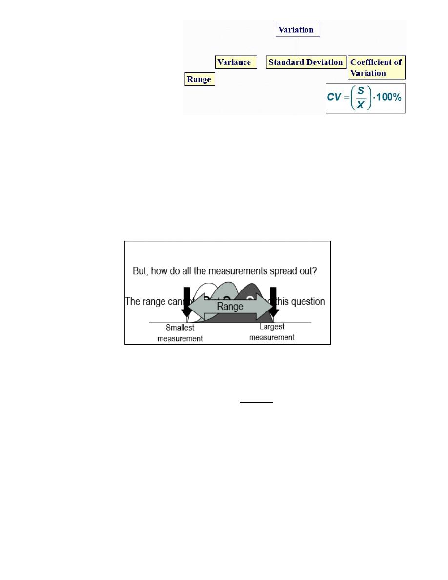
Measures of Variation
1.The range
A. The range of a set of measurements is the difference between the largest and smallest
measurements.
B. Its major advantage is that it is easy to calculate.
C. Its major limitation is its failure to provide information on the spread of the values between
the two end points.
2.Interquartile Range (IQR)
Interquartile Range (IQR)= Q
3
− Q
1
The quartiles are the three numbers that divide the ordered data into four equally sized groups.
Q
1
has 25% of the data below it.
Q
2
has 50% of the data below it. (Median)
Q
3
has 75% of the data below it.
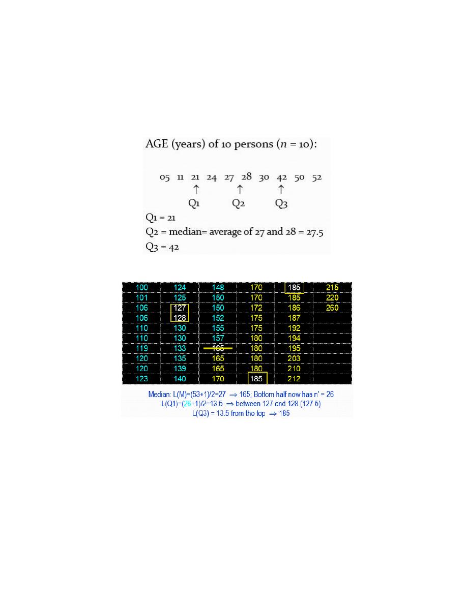
Calculation of the Quartiles
Order the data.
Find the median (also called Q
2
)
The “median” of the lower half of the data = Q
1
The “median” of the upper half of the data = Q
3
Example:
Example: weight data n = 53
Calculation of Interquartile Range (IQR)
Q
1
= 127.5
Median = 165
Q
3
= 185
Interquartile Range (IQR)= Q
3
− Q
1
= 185 – 127.5= 57.5
IQR gives the spread of middle 50% of the data points
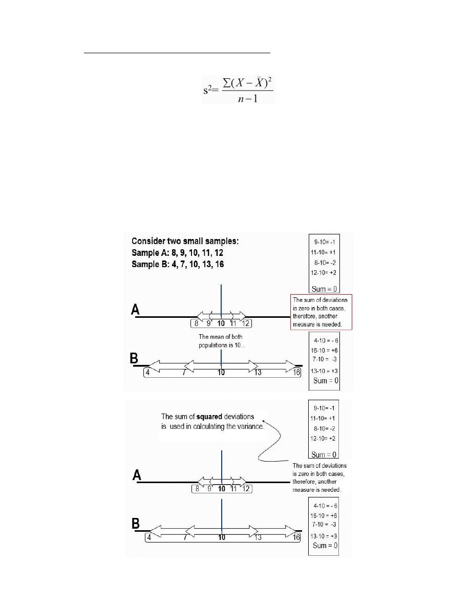
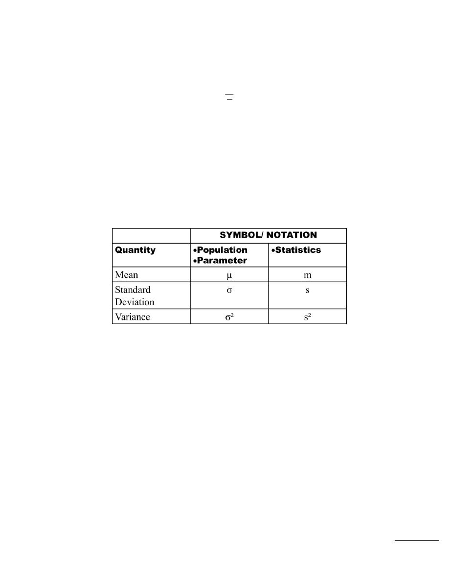
3.The Variance ( S
2
)
Variance is the Average squared deviation from the mean (i.e. the average squared distance from the
Mean)
Calculation of the Variance
Calculate the mean
Find the deviation of each value (Subtract each observation from the mean)
Square the deviations
Sum the squared deviations: this is called the sum of squares (SS)
Divide the SS by n-1
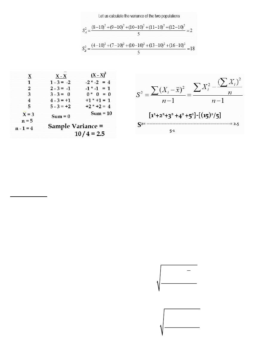
Variance Example
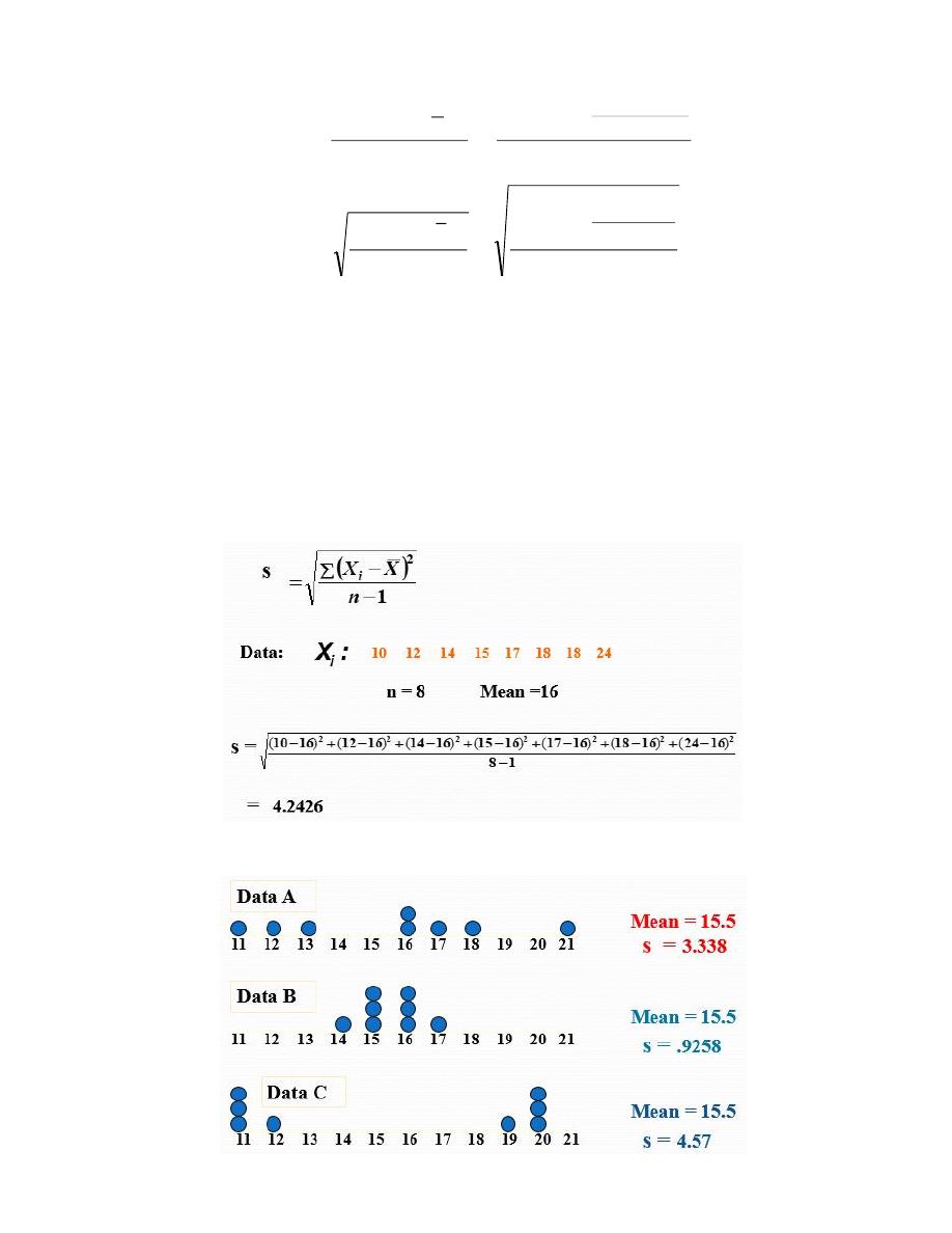
4.Standard Deviation (S or SD)
➢ The standard deviation is the average variability (distance) from the Mean
➢ It is the square root of variance
SD Properties:
A. It is the most important measure of variation
B. It has the same units as the original data
Calculation of Standard Deviation
Calculate the Variance
Take the square root
Sample standard deviation:
Population standard deviation:
(
)
2
1
1
n
i
i
X
X
S
n
=
−
=
−
(
)
2
1
N
i
i
X
N
=
−
=
Variance and standard deviation
Interpreting Standard Deviation
⚫ The standard deviation can be used to
– compare the variability of several distributions
– make a statement about the general shape of a distribution.
Example
Comparing Standard Deviations
1
)
(
1
)
(
2
2
2
2
−
−
=
−
−
=
n
n
X
X
n
x
X
S
i
i
i
1
)
(
1
)
(
2
2
2
−
−
=
−
−
=
n
n
X
X
n
x
X
S
i
i
i
5.The coefficient of variation
The coefficient of variation is the standard deviation divided by the mean value.
It is a measure of relative variation rather than absolute variation as standard deviation
Choosing Summary Statistics
Use the mean and standard deviation for reasonably symmetric distributions that are free of
outliers.
Use the median and IQR when data are skewed or when outliers are present.
Terminology
Thank You
100
=
x
s
CV