
The concepts of
probability

LEARNING OBJECTIVES
At the end of the lecture the student should:
1. Be able to understand the b
asic
concepts of probability
.
2. know and apply laws of Probability.
3. know the characteristics of the normal
distribution .
2

4.
5.
know the
Standard Normal
Distribution curve (z distribution) and
understand what is meant by a z score.
be able to perform normal calculations,
both finding areas under the curve and
percentages where the area under the
curve is given.
3

Definitions
•
•
•
Probability
is a numerical measure of
the likelihood that an event will occur.
An
experiment
is any process that
generates well-defined
outcomes
.
Sample space,
S
,
is the set of all
possible outcomes of an experiment.

Definitions
•
•
An
event
,
A
,
is an outcome or set of
outcomes that are of interest to the
experimenter (An event A is a subset
of the sample space.
The
probability of an event A, P(A),
is a
measure of the likelihood that an event
A
will occur.

Example – Tossing a Coin
•
•
S = {H, T}
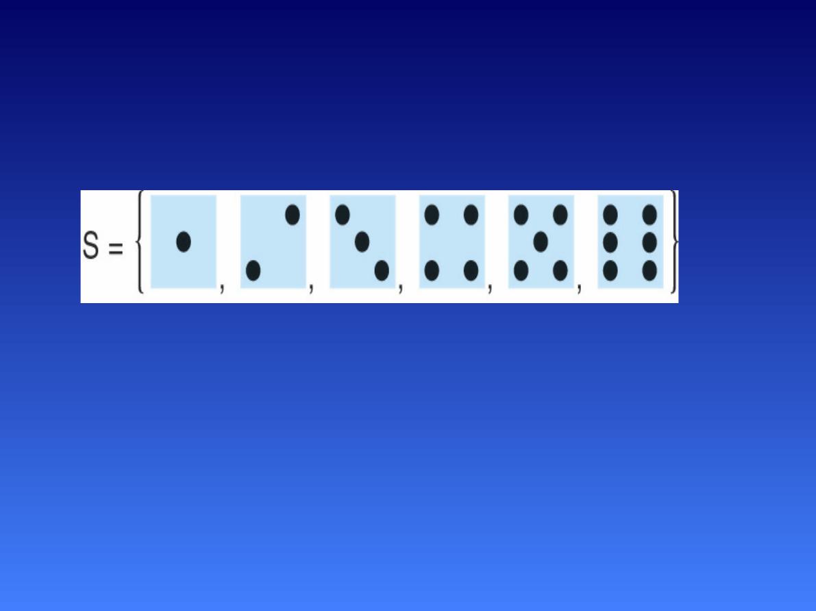
Example – Tossing a Dice
•
•
•
S = {1, 2, 3, 4, 5, 6}
A = {roll an even number}
A = {2, 4, 6}

•
•
•
Calcula on of Probability
In classical probability each outcome is
equally likely
In these cases, if there are
N
outcomes in
S then the probability of any one outcome
is 1/
N.
If A is any event and
n
A
is the number of
outcomes in A, then
A
P A
n
N

Example – Tossing a Dice
•
•
•
S = {1, 2, 3, 4, 5, 6}.
The 6 outcomes are equally likely, i.e., P(1)
= P(2) = P(3) = P(4) = P(5) = P(6) = 1/6.
A = {roll an even number} = {2, 4, 6}.
3
P A
0 .5
6

Empirical probability
•
•
It is simply the relative frequency that
some event is observed to happen (or
fail)
Number of times an event occurred
divided by the number of trials

Relative Frequency Example
•
•
•
•
•
•
•
•
#Children Freq Relative. frequency
0 40 -
1 80 80/215= 0.37
2 50 -
3 30 -
4 10 -
5 5 -
sum 215

Basic Concepts of
Probability
•
•
•
Probability values are always assigned
on a scale from 0 to 1.
A probability near 0 indicates an event
is very unlikely to occur.
A probability near 1 indicates an event
is almost certain to occur.

Basic Concepts of
Probability
•
•
A probability of 0.5 indicates the
occurrence of the event is just as
likely as it is unlikely.
The sum of the probabilities of all
outcomes is 1.

Laws of Probability

1.Law of Addition
Probability of one event
or
another
If A and B are mutually exclusive
events( A&B can't occur at the same
time) , then
P(A
or
B) = P(A) + P(B) – P(A and B)
P(A
or
B) = P(A) + P(B)

Mutually exclusive events:
Occurrence of one event precludes the
occurrence of the other event
Independent events:
Occurrence of
one event does not affect the
occurrence or non occurrence of the
other event

2.Law of Multiplication
What is the probability that both A and B
occur together?
P(A
and
B) = P(A) x P(B)

Probability Distribution
•
•
X
Probability Distribution is defined as
the distribution of all possible
outcomes of a particular event.
Examples of probability distributions
are:
the binomial distribution (only two
statistically independent outcomes
are possible on each attempt) .

X
X
The normal distribution
other distributions exist (such as the
Poisson, t, F, chi-square, etc.) that
are used to make statistical
inferences.

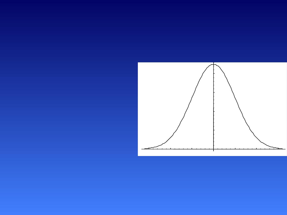
The Normal Distribution Curve
•
•
The characteristics of the Normal
distribution curve
The normal curve is
bell-shaped
and
has a single peak at the exact center
of the distribution.
The arithmetic mean, median, and
mode of the distribution are equal and
located at the peak.

•
•
•
•
The normal probability distribution is
symmetrical about its mean ( half the
observations are above the mean, &
half below the mean.
It is determined by two quantities the
mean & the standard deviation
The random variable has an infinite
theoretical range (Tails don’t touch X
axis)
The total area under the curve is equal
to
1

•
•
•
68% of the area under the curve is
between the mean ±1 SD.
95% of the area under the curve is
between mean±1.96 SD.
99% of the area under the curve is
between mean±2.58 SD.
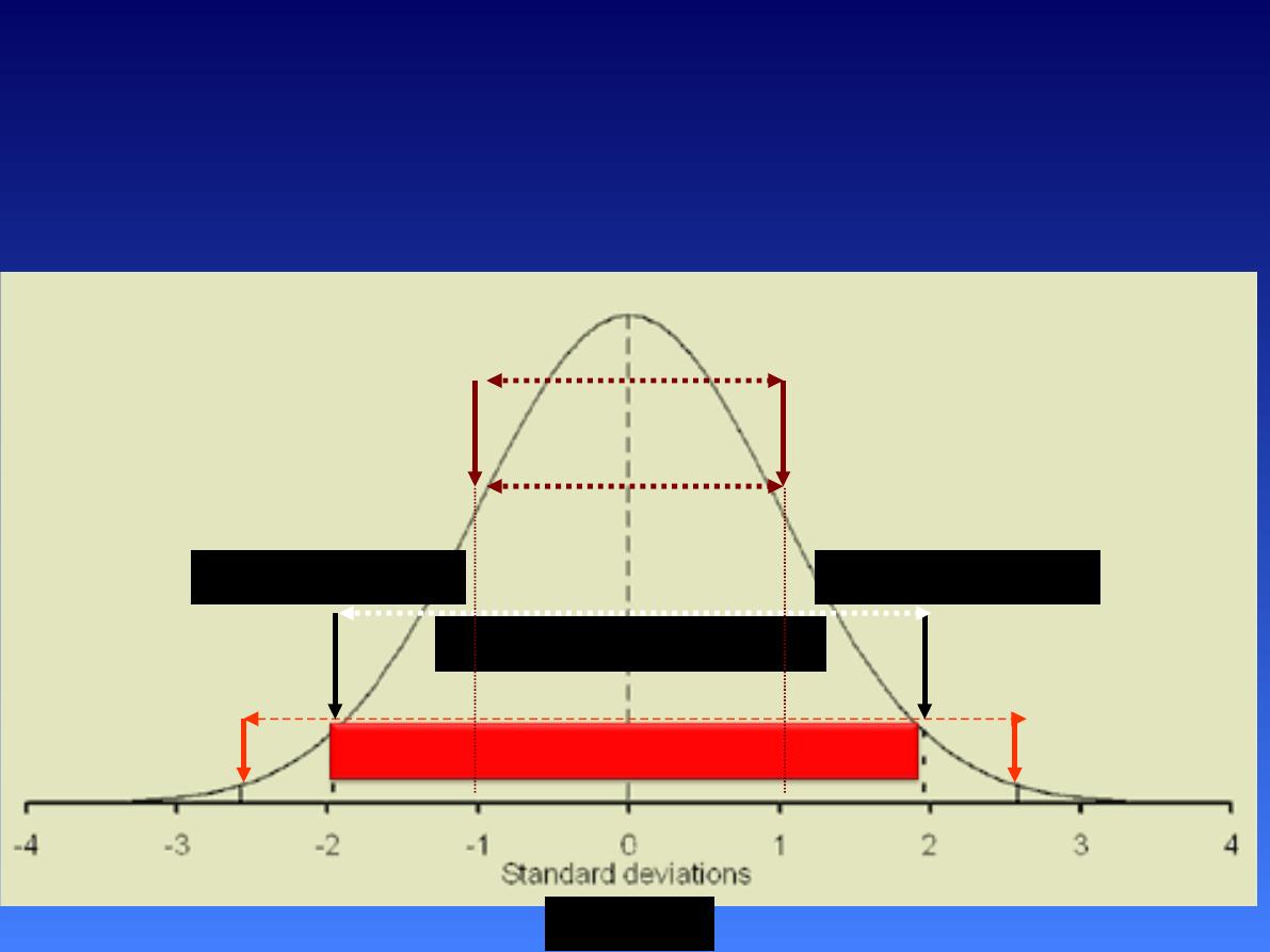
The Normal Distribution
Mean-2.58 SD
Mean+2.58 SD
95% of the area
Mean +1.96 SD
Mean -1.96 SD
99% of the area
68% interval
Mean
Mean -1 SD
Mean +1 SD

Why the Normal Distribution
is Important
•
The normal distribution is a very
important probability distribution in
statistics Because:
Many types of data that are of interest
have a normal distributions (height of
adults, weight of children , intelligence)

•
•
Means of any distribution has a
Normal distribution (Central Limit
Theorem) . Sampling distribution of
means becomes normal as N
increases, regardless of shape of
original distribution
Binomial becomes normal as N
increases.
Standard Normal Distribution
curve (z distribution)
• A normal distribu on
with a mean of 0 and
a standard devia on
of 1 is called the
standard normal
distribu on.
-3
-2
-1
1
2
3

•
•
Any normal distribution can be
converted to the standard normal
distribution using the
Z statistic
.
Z value (score):
The distance between
a selected value, designated
X,
and the
mean , divided by the standard
deviation.
sd
x
x
z
i

Z-Scores
•
•
A
z score
is often called the
standardized value or Standard Normal
Deviate (SND)
.It represents the number
of standard deviation a data value x is
away from the mean and in which
direction.
A data value less than the sample mean
will have a z-score less than zero (has a
minus sign).

•
•
•
A data value greater than the sample
mean will have a z‐score greater than zero
(has a posi ve sign).
A data value equal to the sample mean
will have a z‐score of zero.
Formula:
s
x
x
z
i

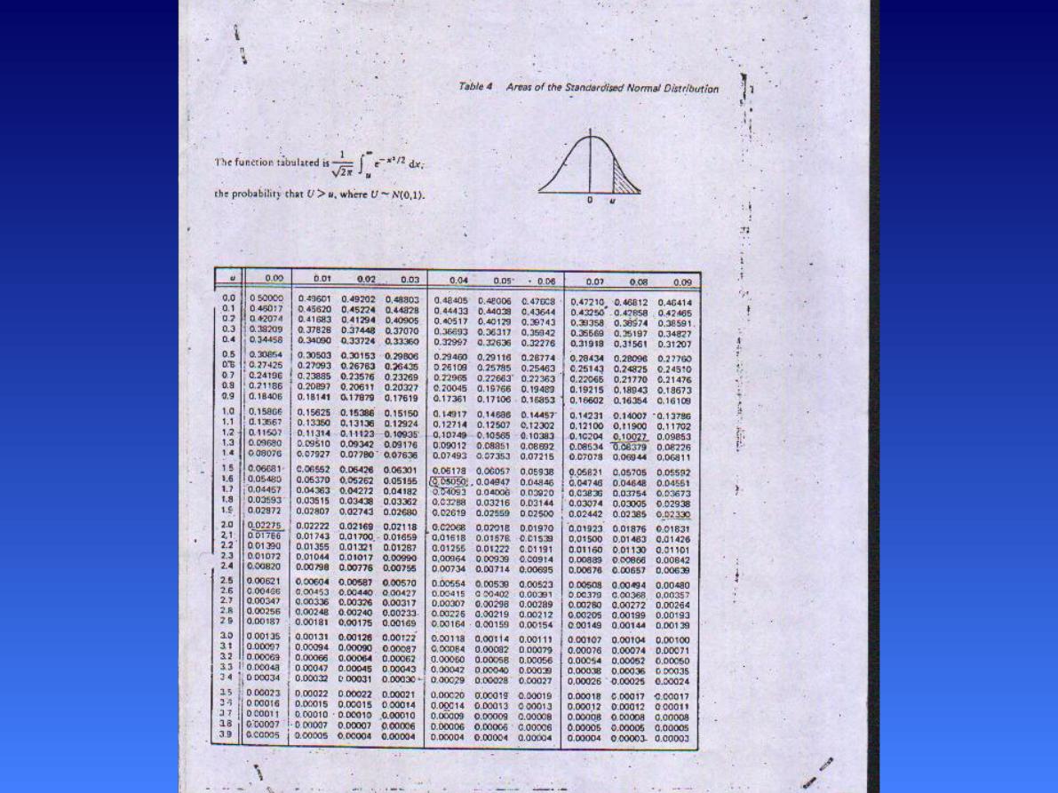
z-Scores (cont)
•
•
The formula changes a “raw” score (x)
to a standardized score (Z).
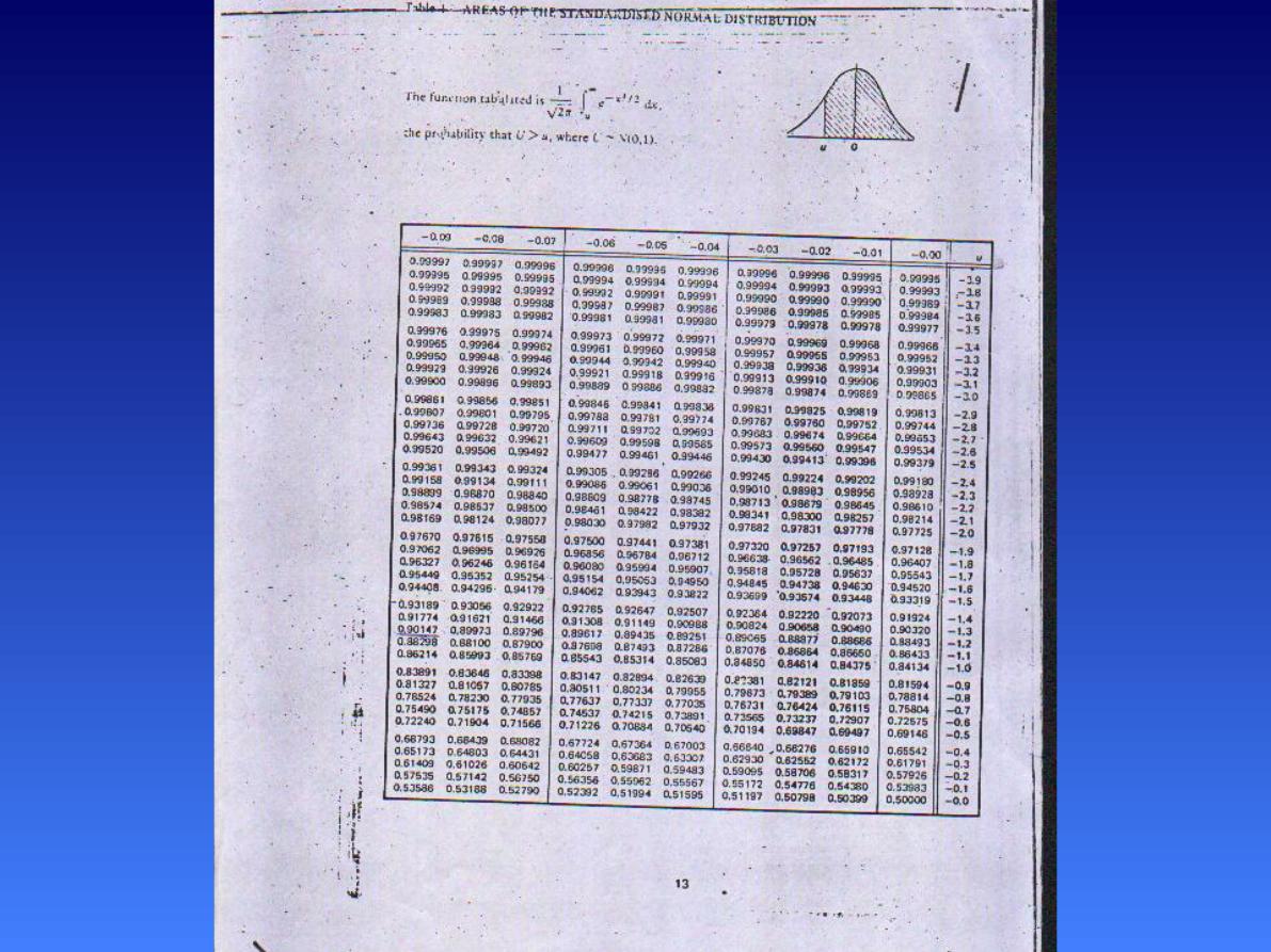
The Z-score can be used to determine
an area under the curve which is
known as a probability by using the
standard distribution table

Example Z Score
•
•
Calculate the Z score for blood pressure
of 140 if the sample mean is 110 and the
standard deviation is 10
Z = 140 – 110 / 10 = 3

Using the Normal Curve: Z
Scores
•
•
•
•
Procedure:
First calculate the Z score(Convert raw
score to Z score), taking careful note
of the sign of the score.
Draw a normal curve
-Indicate where Z score falls
- Shade area in which you are
interested (you are trying to find).
Use the standard distribution table

1-Determine the percentage above
or below a Z score
•
•
1.
2.
Example:
After an exam, you learn that the
mean for the class is 60, with a
standard deviation of 10. Suppose
your exam score is 70.
What is your Z-score?
What percentage of students have a
score below your score? Above?
To solve:
•
•
Available information:
X
i
= 70
= 60
S = 10
Formula:Z = (X
i
– ) / S
= (70 – 60) /10
= +1.0

•
•
•
•
The Z-score of +1.0 is exactly 1 sd
above the mean.
From the table the probability above z
+1.0 = 0.1587
(% of marks above 70= 15.87%)
Therefore the probability below z +1.0
= 1-0.1587 =0.8413.
(% of marks below 70= 84.13%).
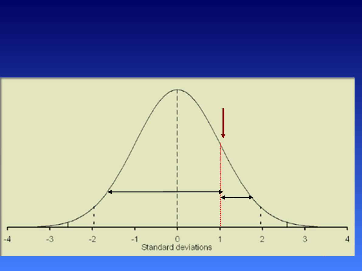
The Standard Normal
Distribution
60
Z=
+1
p= 0.1587
p= 0 .8413.
70

What if your mark is 55%?
1.
2.
Calculate the Z-score.
What percentage of students have a
score below your score? Above?

Answer:
•
•
Z = (55 – 60) /10 = -0.5
Area above Z=-0.5 = 0.6915
(% of marks above 55= 69.15%)
The area below Z = 1-0.6915=0.3085
(% of marks below 55=30.85%)
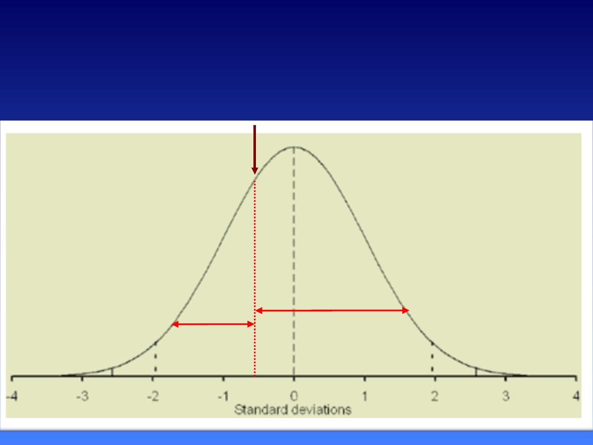
The Standard Normal
Distribution
60
Z=
-0.5
55
P=0.3085
P= 0.6915

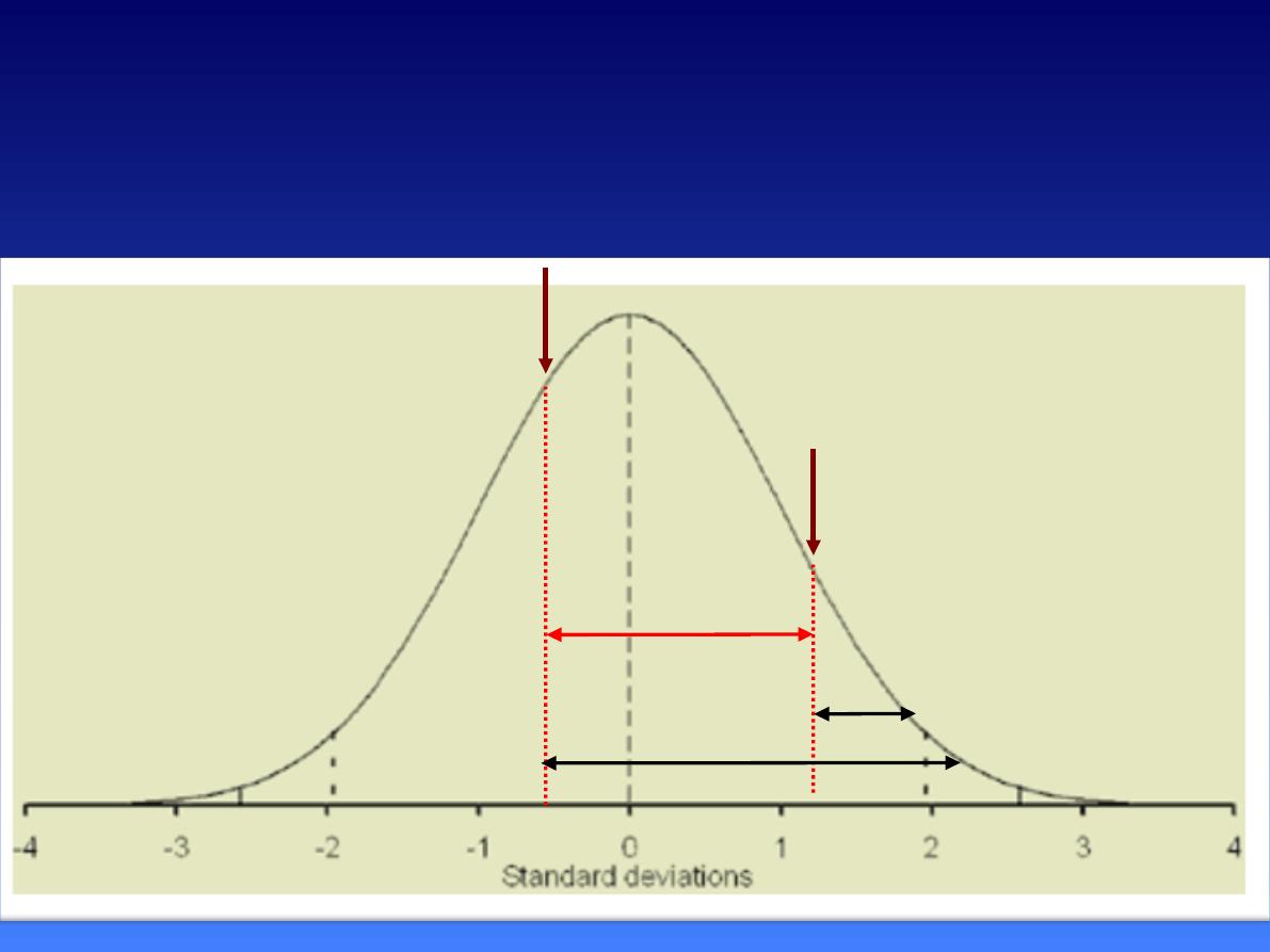
2-Determine the percentage between 2
Z scores
•
•
Suppose your score is 72 and your
classmate has 55.
What is the probability of someone
having a mark between your score and
your classmate’s?

Answer:
•
•
•
•
Z for 72 = (72 – 60) /10 = +1.2
The area above Z 1.2 =0.1151
Z for 55% = (55 – 60) /10 = -0.5
The area above Z -0.5= 0.6915
The area between Z = 1.2 and Z = -0.5
would be 0.6915 -0 .1151 = 0.5764

• The probability of having a mark
between 72 and 55 for this distribution
is p =0 .5764 or 57.64%
44
The Standard Normal
Distribution
60
Z=
-0.5
Z=
+1.2
55
72
P=
0.5764
P=
0.6915
P=
0 .1151

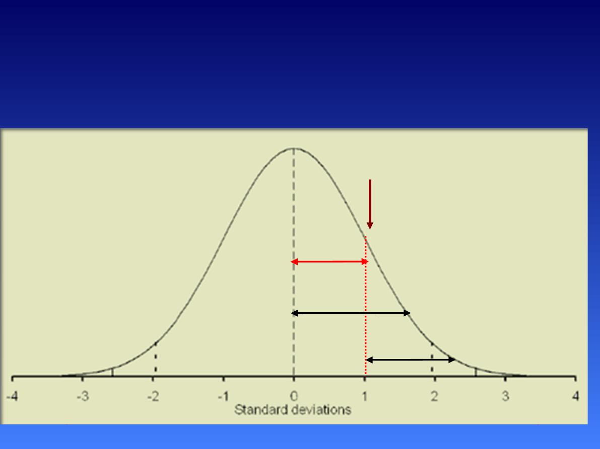
3-Determine the percentage of
scores between the mean and
particular z score
•
•
What is the probability of having a
mark between 60% and 70%?
The area above Z score 1=0.1587
0.5-0.1587=0.3413
There is a 0.3413 probability (or
34.13% chance) of having a mark
between 60 and 70.
The Standard Normal
Distribution
60
Z=
+1
p= 0.1587
70
p= 0.5
p= 0.3413

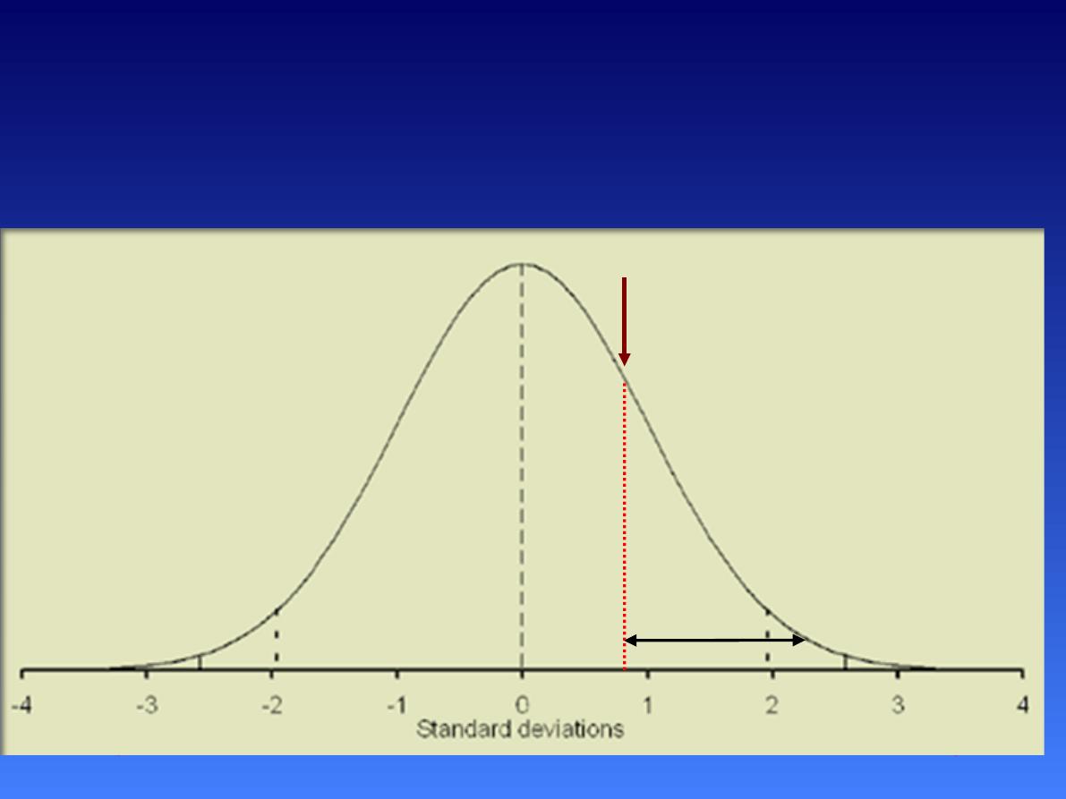
•
•
4‐ Steps for determining a Z score or
raw score from percentage
(propor on)
If, instead, we are given a propor on and
asked to find the original value of
x
corresponding to it?
Draw normal curve ,shade approxima on
area for percentage desired
The Standard Normal
Distribution
100
Z=
+0.84
p= 0.2
116.8

•
•
•
We have to use the Table backwards!
What propor on are we interested in?
Look inside the body of the Table for the
value closest to this “propor on. That will
give us a
z
score. Then the original value
of
x
is simply
.
zsd
x
x

example
•
•
•
For a normal distribution with mean of
100 and standard deviation of 20, find the
score that cuts the upper 20% .
From the table Z=0.84
0.84=
x-
100/20
X=20*0.84+100=116.8

52
Chapter 7 Probability
Thank You