

The Binomial Distribution

Binomial Experiment
!
The binomial experiment can result in only
one of two possible outcomes.
!
Typical cases where the binomial experim
ent applies:
"
A coin flipped results in heads or tails
"
A sick person improves or dies
"
A pregnant woman gives birth to male or female
baby
December 4, 2011

Binomial Experiment
!
Characteristics of a Binomial Experiment:
1. The experiment consists of n identical trials (n is
finite and fixed).
2. There are only two possible outcomes on each tr
ial,
may be labeled as
“success”
and
“failure
”
3. The probability of success stays the same for
each trial. The probability of success is denote
d by p.
4. The trials are independent.

!
Definitions
"
Binomial Random Variable:
The binomial random variable is the number of su
ccesses in
n
trials of the binomial experiment.
“By definition, this is a discrete random variable”.
"
The Binomial probability distribution:
The Binomial probability distribution
is the discre
te probability distribution of the number of succe
sses in a series of n trials, each of which yields
success with probability p.
#
n : the number of trials
#
X or r : the number of observed successes
#
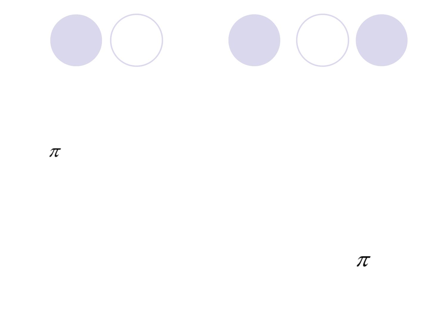
or p: the probability of success of an event on e
ach trial
!
Note:
#
Since success and failure are two mutually exclu
sive events
#
The probability of failure on each trial is 1-
The BINOMIAL DISTRIBUTION
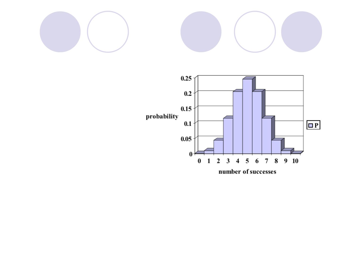
Binomial Distribution
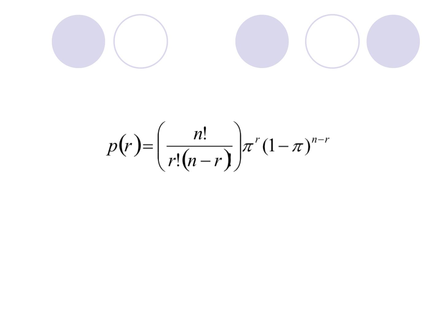
Calculating the Binomial Probability
The binomial probability P(r) is calculated as:
Where r = 0, 1, 2, ..., or n.

The
factorial
notation “
!
”.
The n! = n × (n − 1) × (n − 2) × · · · × 3 × 2
× 1
!
For example: 5! = 5 × 4 × 3 × 2 × 1 = 120
!
Note that 0! = 1, by definition.

EXAMPLE
!
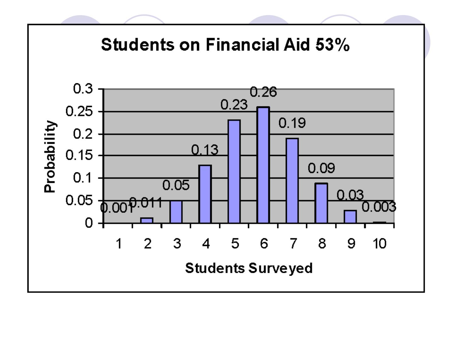
At a college, 53% of students receive financi
al aid. In a random group of 9 students, what
is the probability that exactly 5 of them receiv
e financial aid?
!
p=0.53
(the probability of success for each trial)
!
n=9
(number of trials )
!
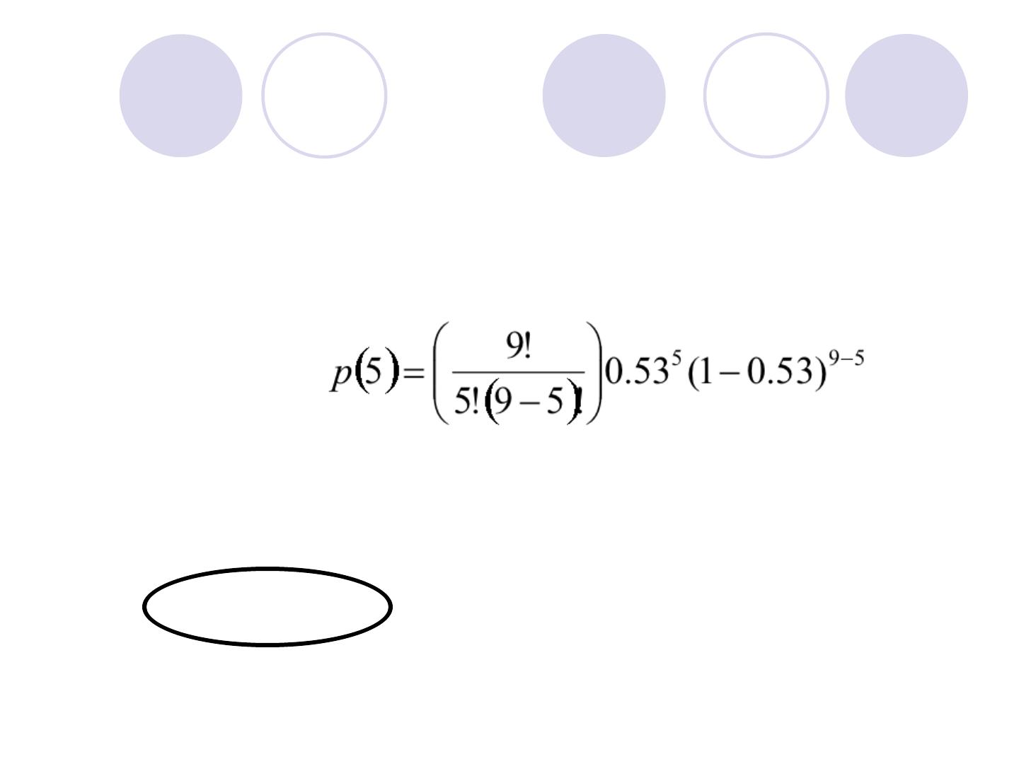
The probability of getting 5 successes (r=5)
EXAMPLE
about 26%

!
P(r=0) = 0 .001
!
P(r=1) = 0.011
!
P(r=2) = 0 .05
!
P(r=3) = 0.13
!
P(r=4) = 0.23
!
P(r=5) = 0 .26
!
P(r=6) = 0.19
!
P(r=7) = 0.09
!
P(r=8) = 0.03
!
P(r=9) = 0.003

!
Draw a diagram of the binomial distribution
for the class of students in the Example
Binomial mean and standard deviation
!
The center and
spread of the
binomial distribution
are defined by the
mean µ and standard
deviation σ
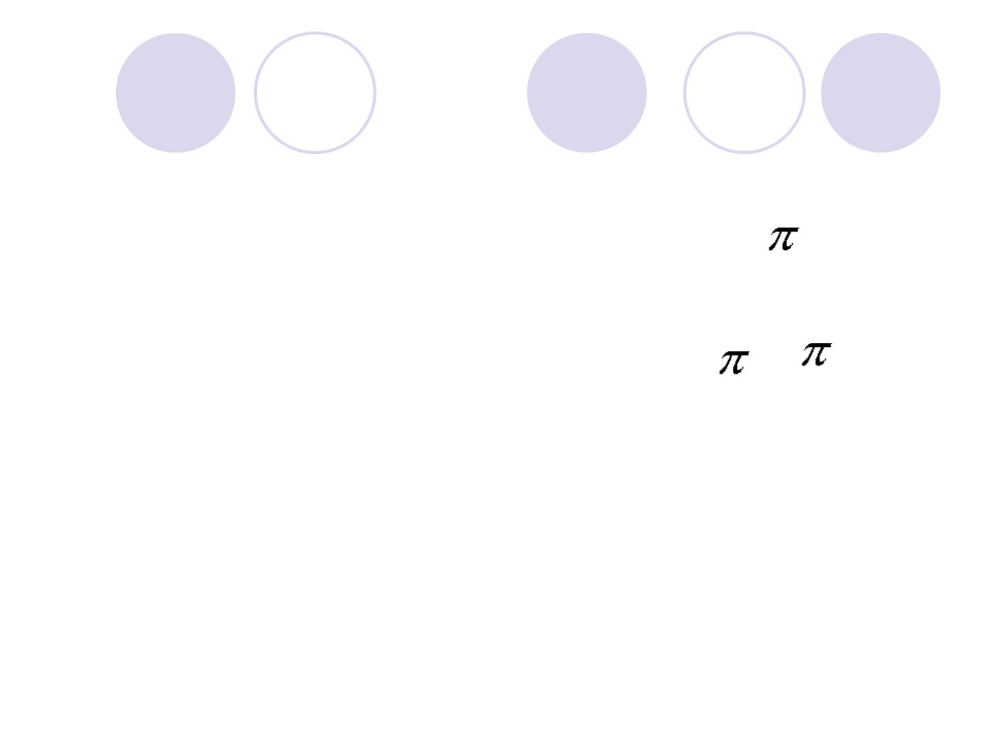
µ = n
!
= √n (1- )
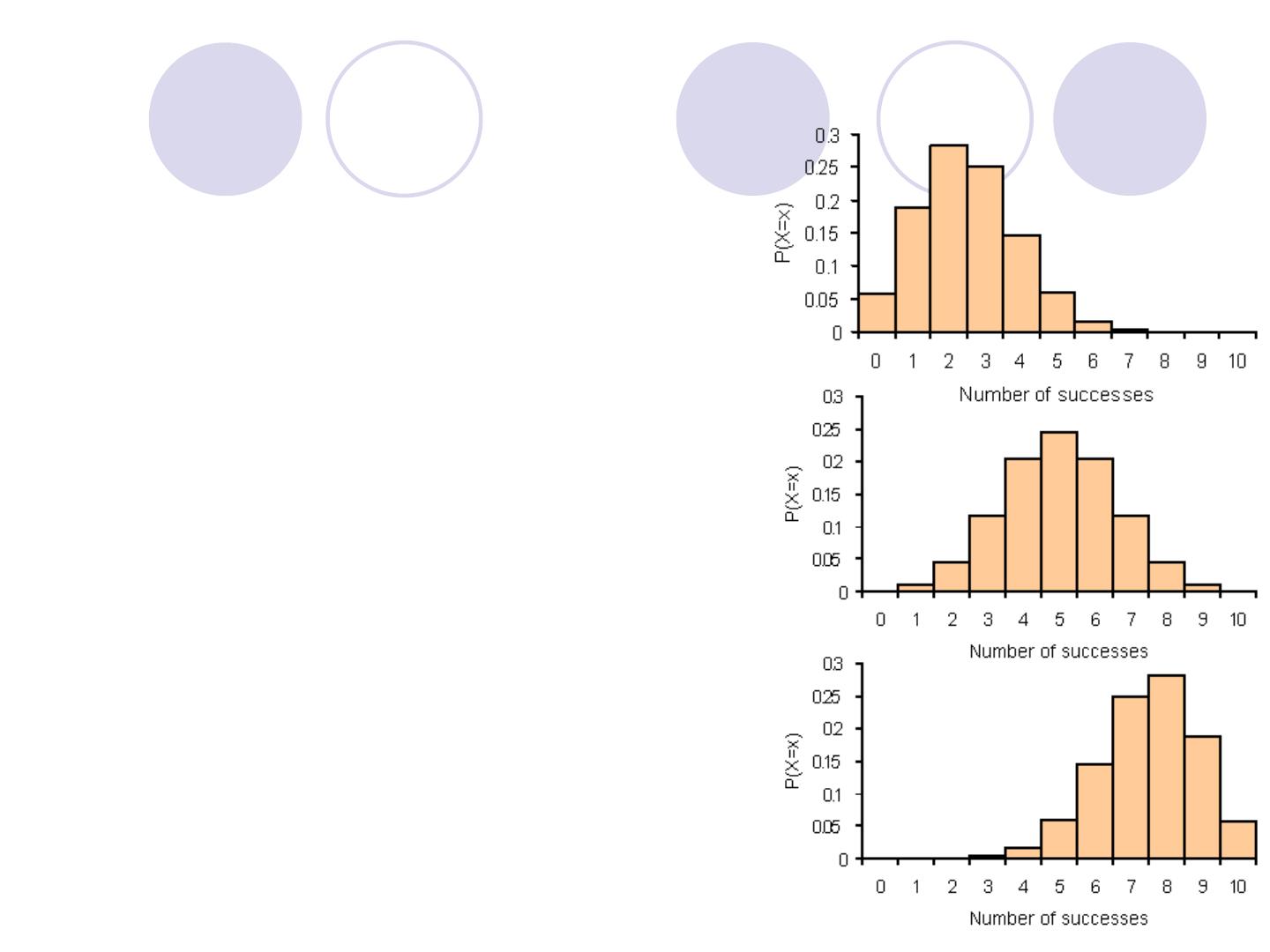
Effect of changing p when
n is fixed.
a) n = 10, p = 0.25
b) n = 10, p = 0.5
c) n = 10, p = 0.75
For small samples, binomial
distributions are skewed wh
en p is different from 0.5.
a)
b)
c)
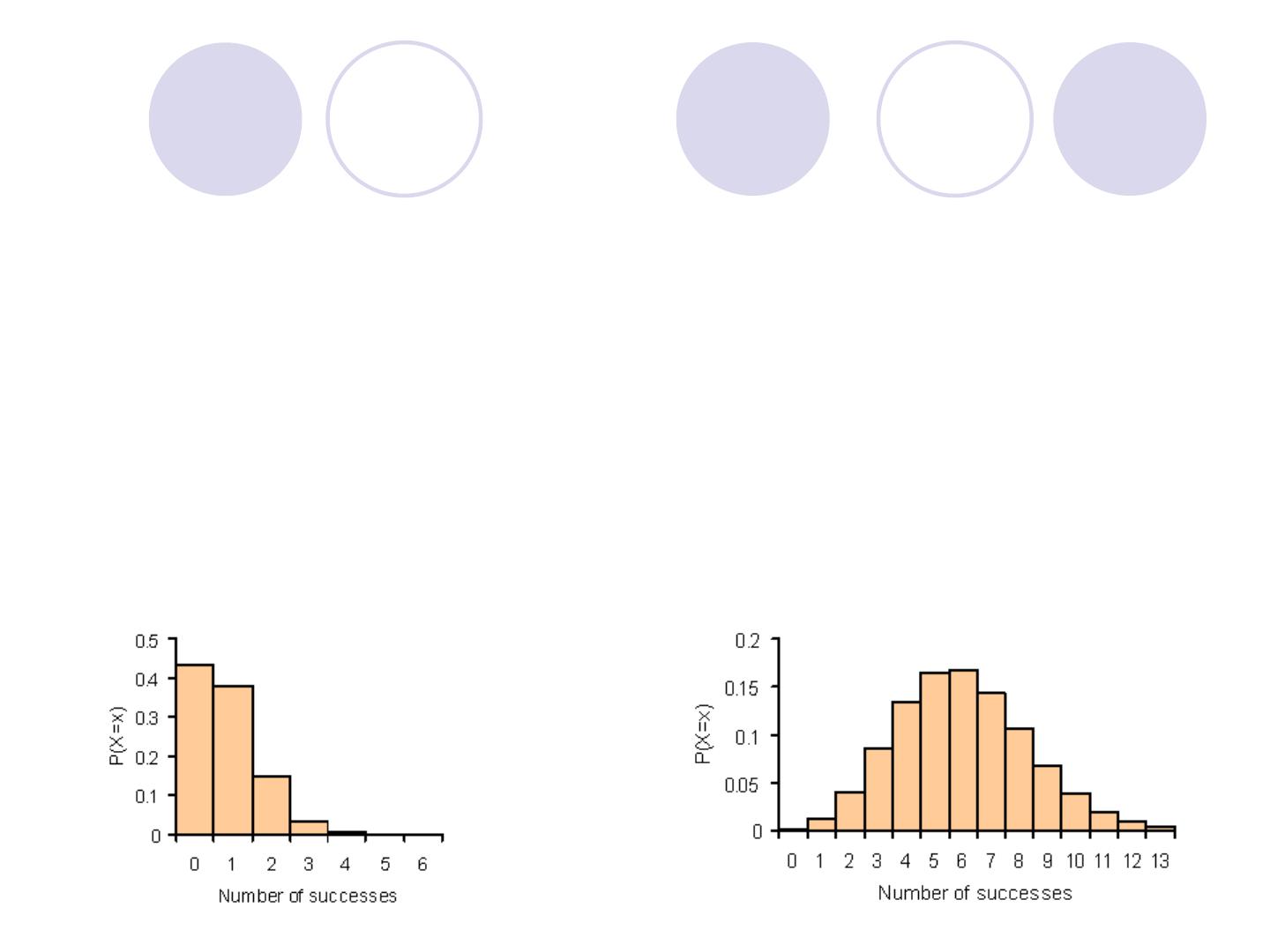
p = .08
n = 10
p = .08
n = 75
µ = 10*0.08 = 0.8
µ = 75*0.08 = 6
σ = √(10*0.08*0.92) = 0.86
σ =
√(75*0.08*0.92) = 3.35
Effect of changing n when p is fixed.
a.
n=10 , p=0.08
b.
N=75 , p=0.08

The Normal Approximation to the Bino
mial Distribution
!
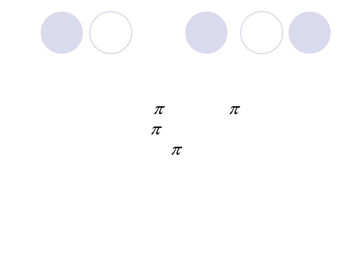
The normal distribution provides a close a
pproximation to the Binomial distribution w
hen :
1.
n (number of trials) is relatively large (As n
increases, a binomial distribution gets clos
er and closer to a normal distribution).
2.
And when p (success probability) is close t
o 0.5.
The Normal Approximation to the Bino
mial Distribution
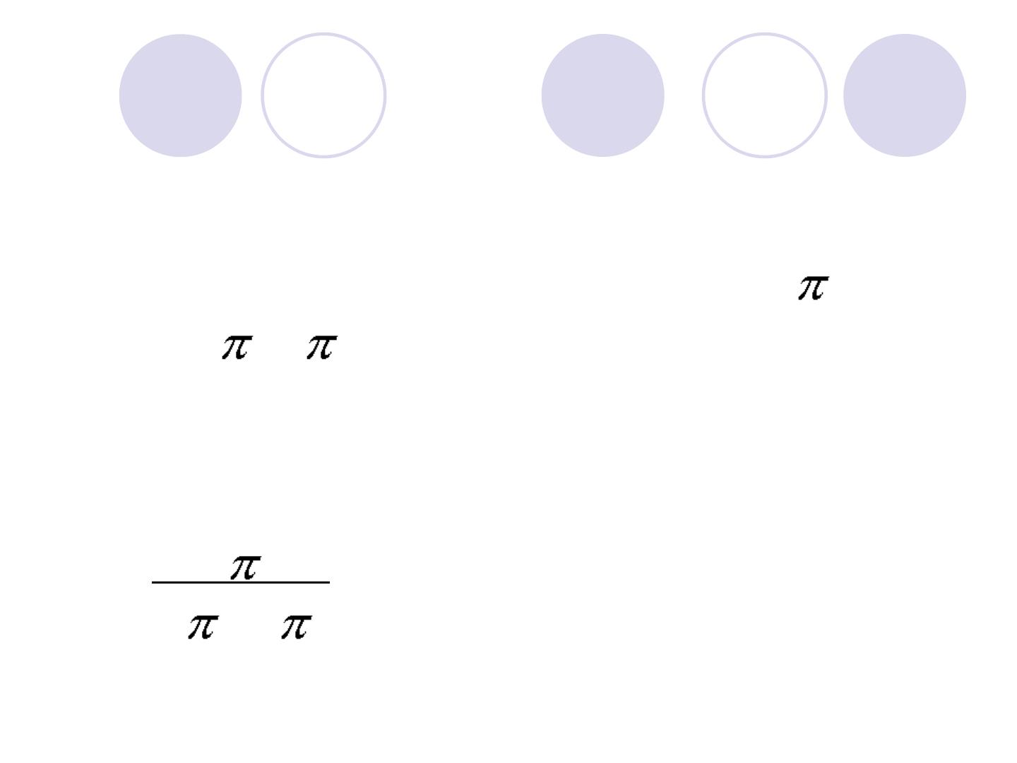
Various rules of thumb may be used to decid
e whether n is large enough. One rule is th
at both n and n(1- ) are both greater tha
n 5. n
" 5
n(1- )
" 5
The Normal Approximation to the Bino
mial Distribution
!
If the assumptions are satisfied, the Binomial
random variable X can be approximated by n
ormal distribution with mean
µ = n
!
!
=
√n (1- )
!
In probability calculations, the continuity corr
ection must be used.
z = r– n____
√n (1- )
Sample proportions
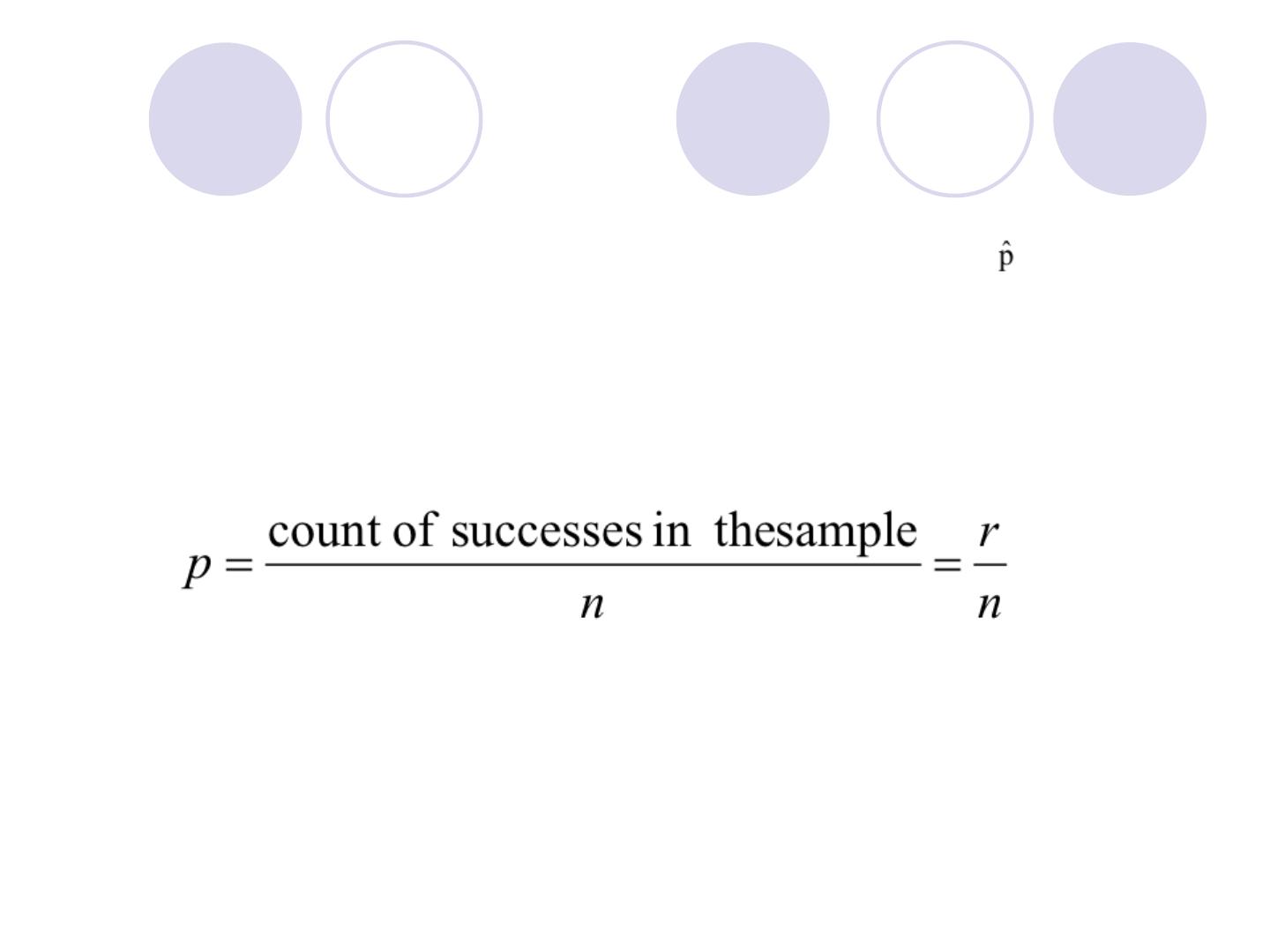
The proportion of “successes” can be more infor
mative than the count.
The sample proportion of successes is:
Z = (p-π) /√ π(1-π)/n
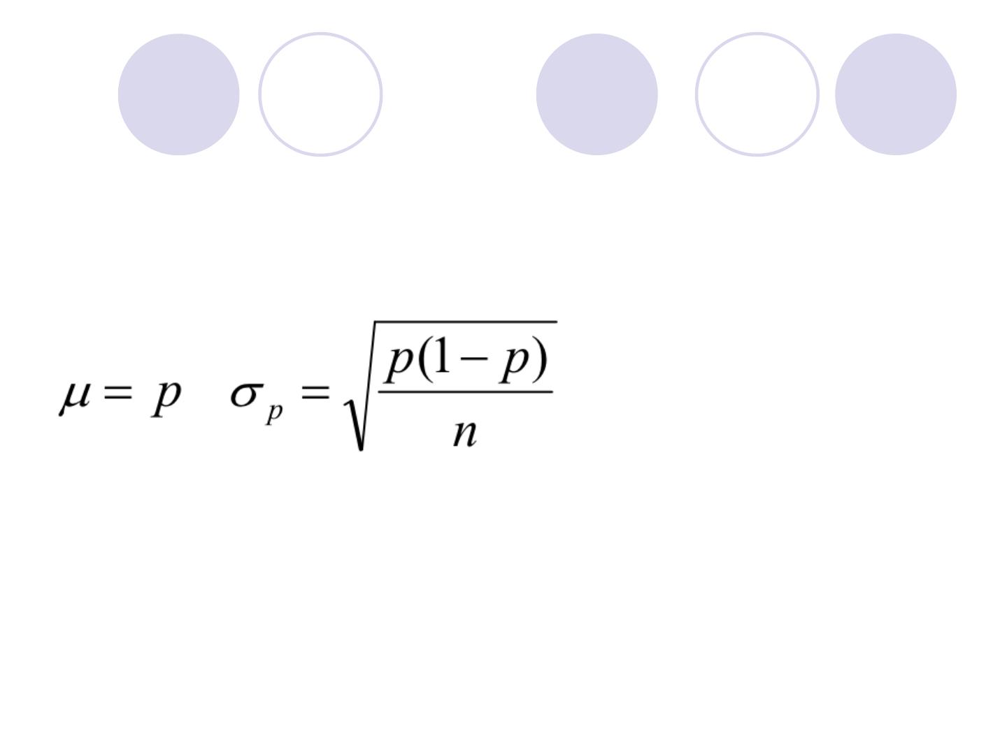
The mean and the standard deviation of
the sample proportion

Example
!
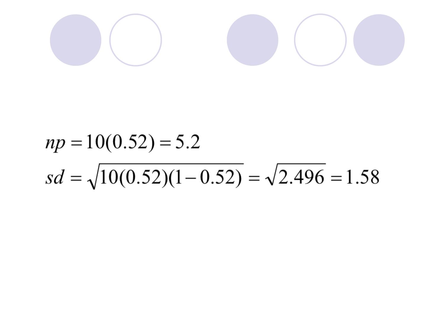
In families of 10 children the proportion of
boys is 0.52. what is the probability of havi
ng a family with 8 boys or more?.

!
we will consider 7.5 +(values above 8) tim
es, and use it to calculate a z-score
z = 7.5 – (10x0.52) = 1.46
1.58
therefore P(r >7.5) = P(z >1.46)
= 0.0722
there is a 7.22% chance of having a family w
ith 8 boys or more.

!
Example: suppose in a certain human population the
proportion of color blindness is 8% (π=0.08). if we ra
ndomly select 150 individuals from this population, w
hat is the probability that the proportion of color blind
ness in the sample will be greater than 0.15 (p=0.15)?
!
Z = p-π / π(1-π)/n = (0.15-0.08) / √0.08(1-0.08)/150
!
!
= 3.15 from z-table
!
Probability = 0.0008.
!