Intro of digital image processing
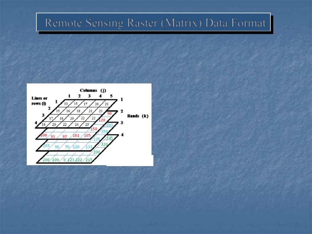
Remote Sensing Raster (Matrix) Data Format
Digital number of column 5,
row 4 at band 2 is expressed
as BV
5,4,2
= 105.
120 150 100 120 103
176 166 155
85 150
85
80
70
77 135
103
90
70 120 133
20
50
50
90
90
76
66
55
45 120
80
80
60
70 150
100
93
97 101 105
210 250 250 190 245
156 166 155 415 220
180 180 160 170 200
200
0 123 222 215
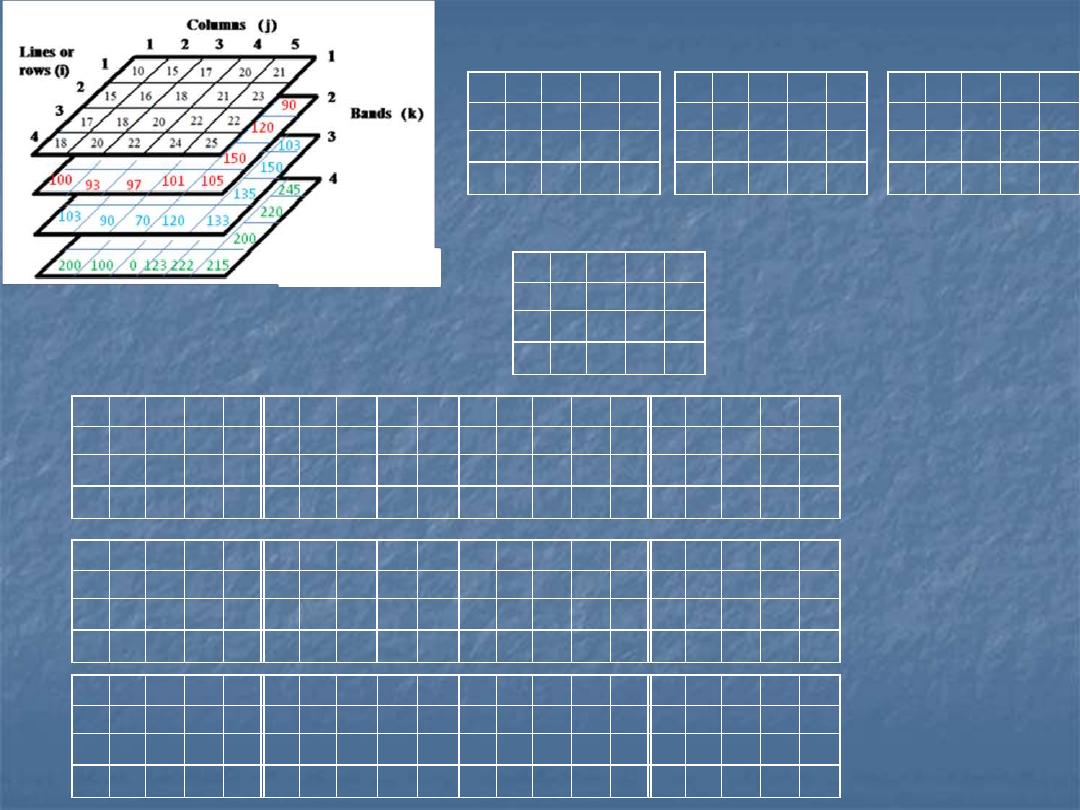
Band 2
Band 3
Band 4
1,1,2 2,1,2 3,1,2 4,1,2 5,1,2
1,2,2 2,2,2 3,2,2 4,2,2 5,2,2
1,3,2 2,3,2 3,3,2 4,3,2 5,3,2
1,4,2 2,4,2 3,4,2 4,4,2 5,4,2
Matrix notation for band 2
10
15
17
20
21
15
16
18
21
23
17
18
20
22
22
18
20
22
24
25
20
50
50
90
90
76
66
55
45 120
80
80
60
70 150
100
93
97 101 105
120 150 100 120 103
176 166 155
85 150
85
80
70
77 135
103
90
70 120 133
210 250 250 190 245
156 166 155 415 220
180 180 160 170 200
200
0 123 222 215
BIL
10
15
17
20
21
20
50
50
90
90
120 150 100 120 103
210 250 250 190 245
15
16
18
21
23
76
66
55
45 120
176 166 155
85 150
156 166 155 415 220
17
18
20
22
22
80
80
60
70 150
85
80
70
77 135
180 180 160 170 200
18
20
22
24
25
100
93
97 101 105
103
90
70 120 133
200
0 123 222 215
BSQ
10
20
120
210
15
15
76
176
156
16
17
80
85
180
18
18
100
103
200
20
50
150
250
17
50
66
166
166
18
55
80
80
180
20
60
93
90
0
22
97
100
250
20
90
120
155
155
21
45
85
70
160
22
70
77
70
123
24
101
120
190
21
90
103
245
415
23
120
150
220
170
22
150
135
200
222
25
105
133
215
BIP
What is image processing
Is enhancing an image or extracting
information or features from an image
Computerized routines for information
extraction (eg, pattern recognition,
classification) from remotely sensed
images to obtain categories of information
about specific features.
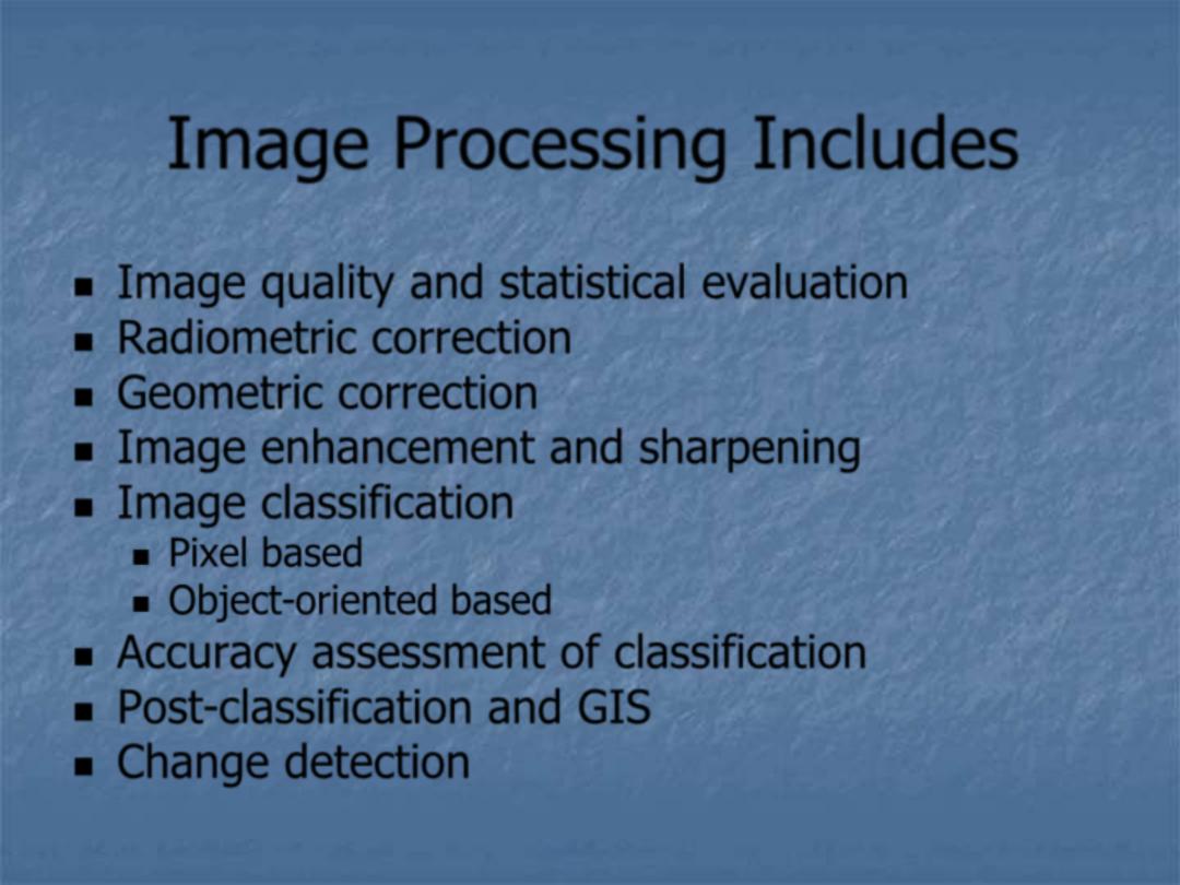
Image Processing Includes
Image quality and statistical evaluation
Radiometric correction
Geometric correction
Image enhancement and sharpening
Image classification
Pixel based
Object-oriented based
Accuracy assessment of classification
Post-classification and GIS
Change detection
GEO5083: Remote Sensing Image Processing and Analysis, spring 2013
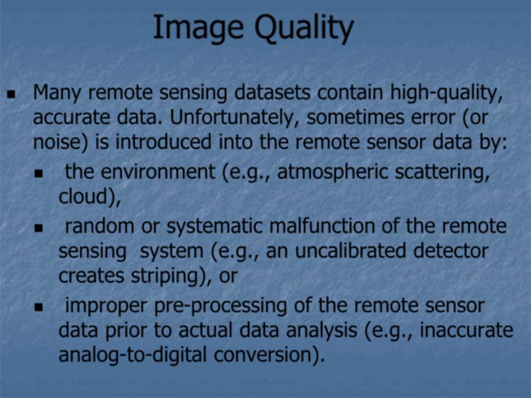
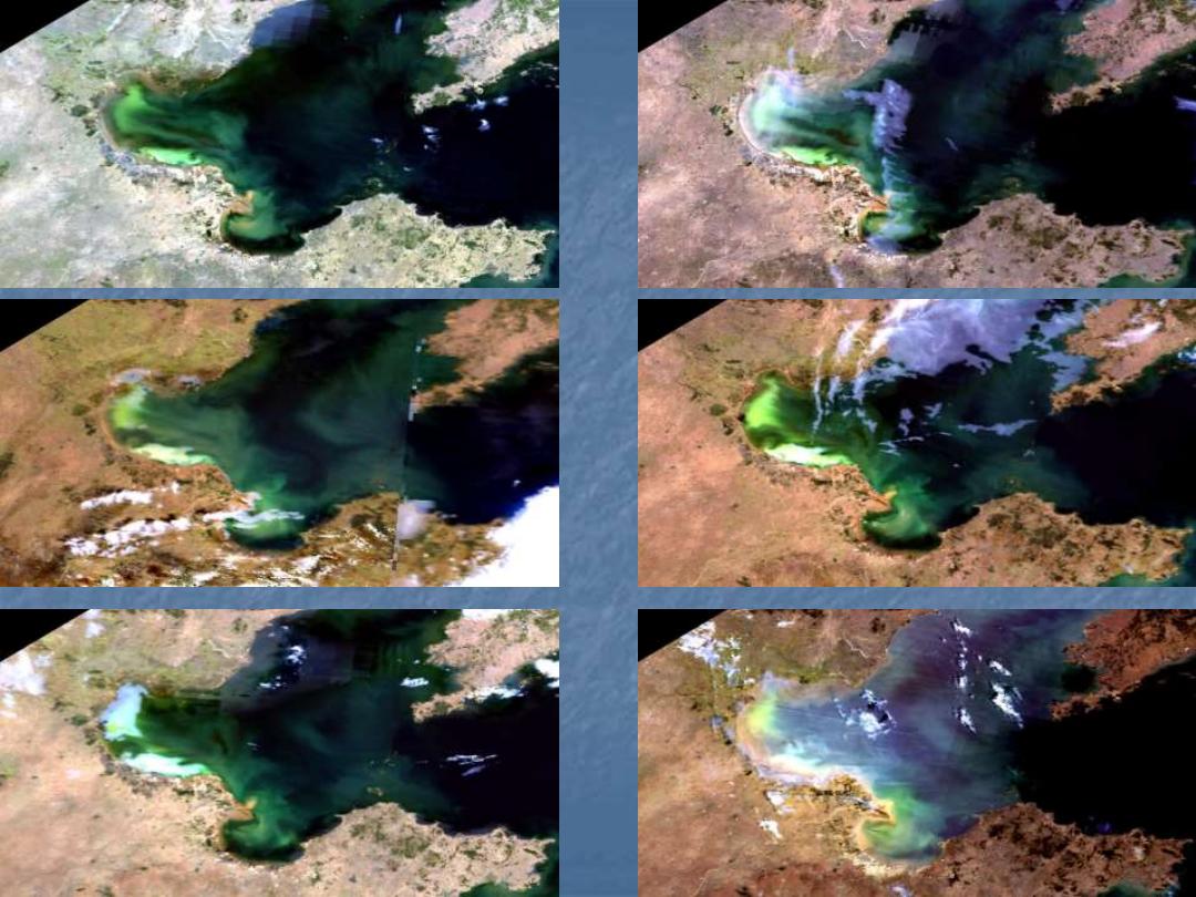
Image Quality
Many remote sensing datasets contain high-quality,
accurate data. Unfortunately, sometimes error (or
noise) is introduced into the remote sensor data by:
the environment
(e.g., atmospheric scattering,
cloud),
random or systematic malfunction
of the remote
sensing system (e.g., an uncalibrated detector
creates striping), or
improper pre-processing
of the remote sensor
data prior to actual data analysis (e.g., inaccurate
analog-to-digital conversion).
155
154
155
160
162
163
164
MODIS
True
143
Cloud
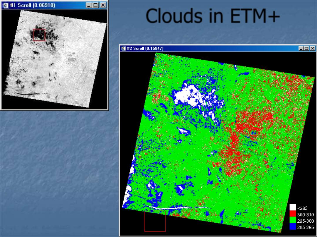
Clouds in ETM+
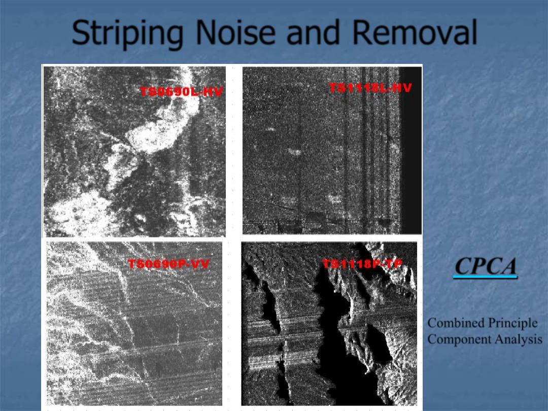
Striping Noise and Removal
CPCA
Combined Principle
Component Analysis
Xie et al. 2004
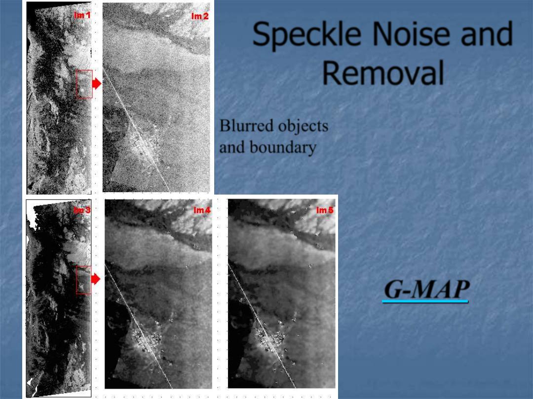
Speckle Noise and
Removal
G-MAP
Blurred objects
and boundary
Gamma Maximum
A Posteriori Filter
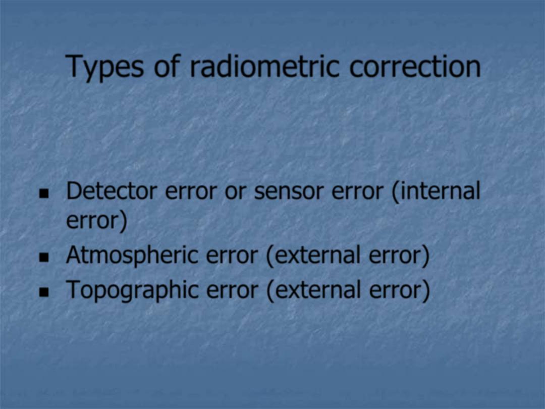
Types of radiometric correction
Detector error or sensor error (internal
error)
Atmospheric error (external error)
Topographic error (external error)
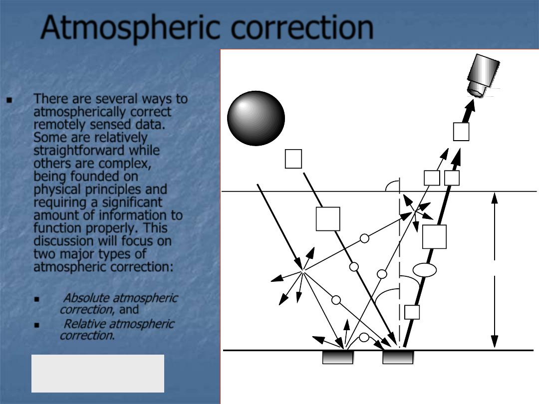
Atmospheric correction
There are several ways to
atmospherically correct
remotely sensed data.
Some are relatively
straightforward while
others are complex,
being founded on
physical principles and
requiring a significant
amount of information to
function properly. This
discussion will focus on
two major types of
atmospheric correction:
Absolute atmospheric
correction
, and
Relative atmospheric
correction
.
Solar
irradiance
Reflectance from
study area,
Various Paths of
Satelli te Received Radiance
Diffuse s ky
irradiance
Total radiance
at the sensor
L
L
L
Reflectance from
neighboring area,
1
2
3
Remote
sens or
detector
Atmosphere
5
4
1,3,5
E
L
90Þ
0
T
v
T
0
0
v
p
T
S
I
n
r
r
E
d
60 miles
or
100km
Scattering, Absorption
Refraction, Reflection
Absolute atmospheric correction
Solar radiation is largely unaffected as it travels through the
vacuum of space. When it interacts with the Earth’s atmosphere,
however, it is selectively
scattered and absorbed
. The sum of
these two forms of energy loss is called
atmospheric attenuation
.
Atmospheric attenuation may 1) make it difficult to relate hand-
held
in situ
spectroradiometer measurements with remote
measurements, 2) make it difficult to extend spectral signatures
through space and time, and (3) have an impact on classification
accuracy within a scene if atmospheric attenuation varies
significantly throughout the image.
The general goal of
absolute radiometric correction
is to turn
the digital brightness values (or DN) recorded by a remote sensing
system into
scaled surface reflectance
values. These
values can
then be compared or used in conjunction with scaled surface
reflectance values obtained anywhere else on the planet.
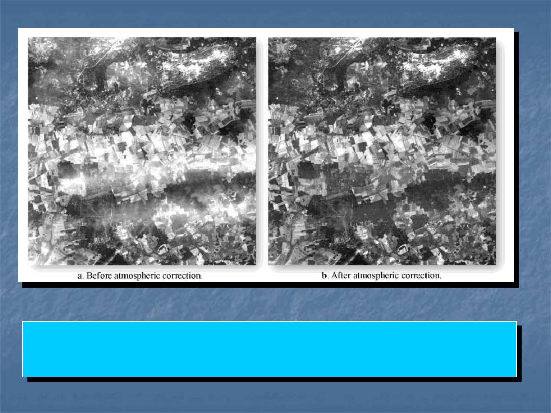
a) Image containing substantial haze prior to atmospheric correction. b) Image after
atmospheric correction using ATCOR (Courtesy Leica Geosystems and DLR, the
German Aerospace Centre).
Topographic correction
Topographic slope and aspect also introduce
radiometric distortion (for example, areas in
shadow)
The goal of a slope-aspect correction is to
remove topographically induced illumination
variation so that two objects having the same
reflectance properties show the same
brightness value (or DN) in the image despite
their different orientation to the Sun’s position
Based on DEM, sun-elevation
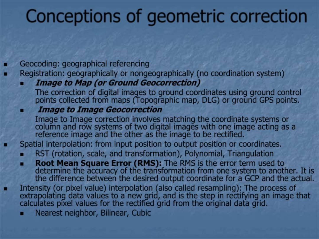
Conceptions of geometric correction
Geocoding:
geographical referencing
Registration:
geographically or nongeographically (no coordination system)
Image to Map (or Ground Geocorrection)
The correction of digital images to ground coordinates using ground control
points collected from maps (Topographic map, DLG) or ground GPS points.
Image to Image Geocorrection
Image to Image correction involves matching the coordinate systems or
column and row systems of two digital images with one image acting as a
reference image and the other as the image to be rectified.
Spatial interpolation:
from input position to output position or coordinates.
RST (rotation, scale, and transformation), Polynomial, Triangulation
Root Mean Square Error (RMS): The RMS is the error term used to
determine the accuracy of the transformation from one system to another. It is
the difference between the desired output coordinate for a GCP and the actual.
Intensity (or pixel value) interpolation (also called resampling):
The process of
extrapolating data values to a new grid, and is the step in rectifying an image that
calculates pixel values for the rectified grid from the original data grid.
Nearest neighbor, Bilinear, Cubic
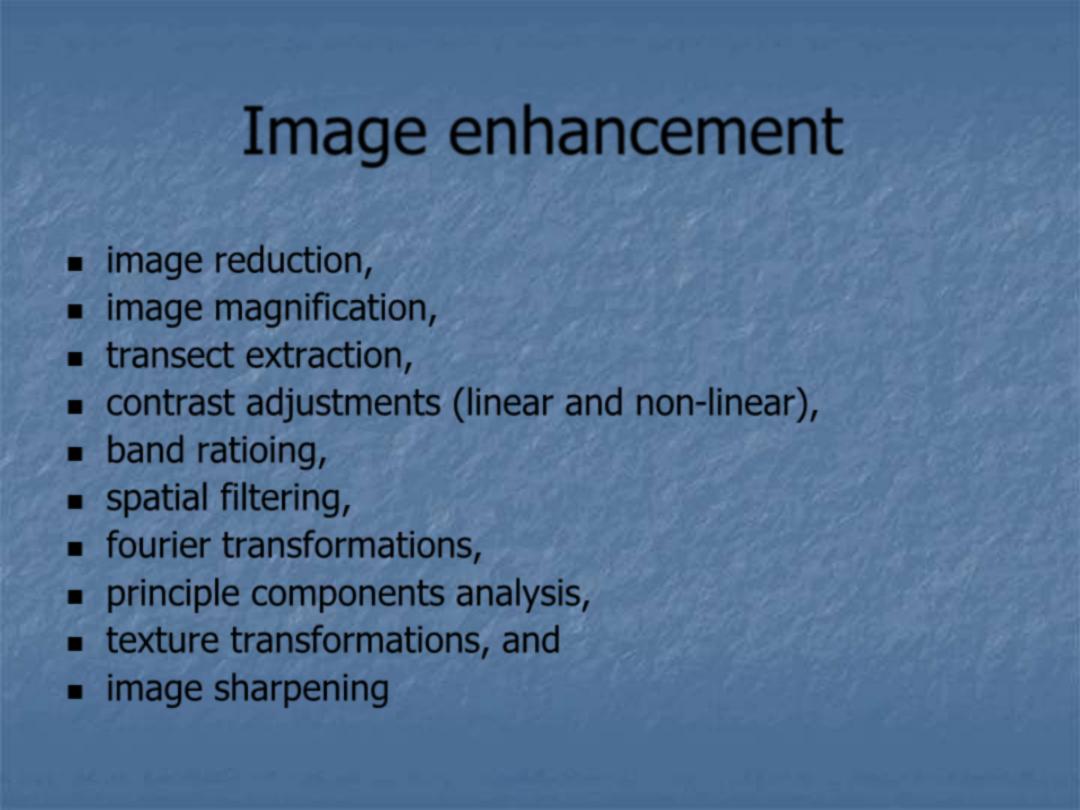
Image enhancement
image reduction,
image magnification,
transect extraction,
contrast adjustments (linear and non-linear),
band ratioing,
spatial filtering,
fourier transformations,
principle components analysis,
texture transformations, and
image sharpening
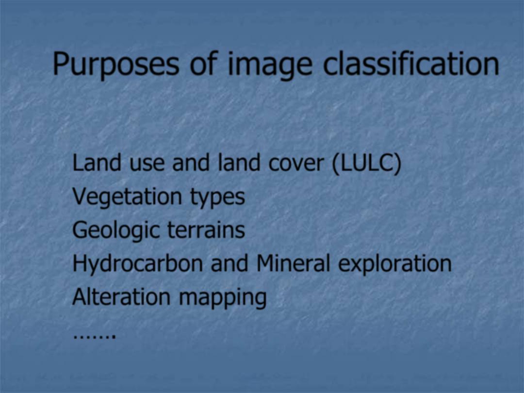
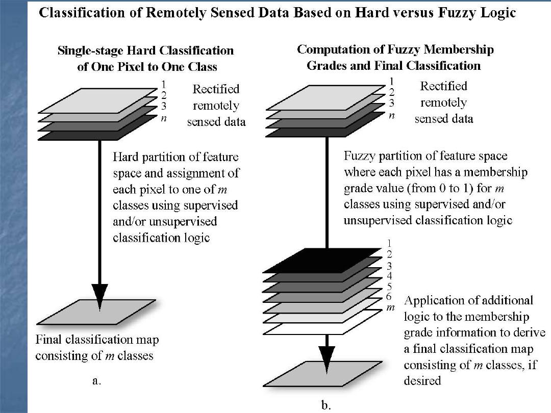
Purposes of image classification
Land use and land cover (LULC)
Vegetation types
Geologic terrains
Hydrocarbon and Mineral exploration
Alteration mapping
…….
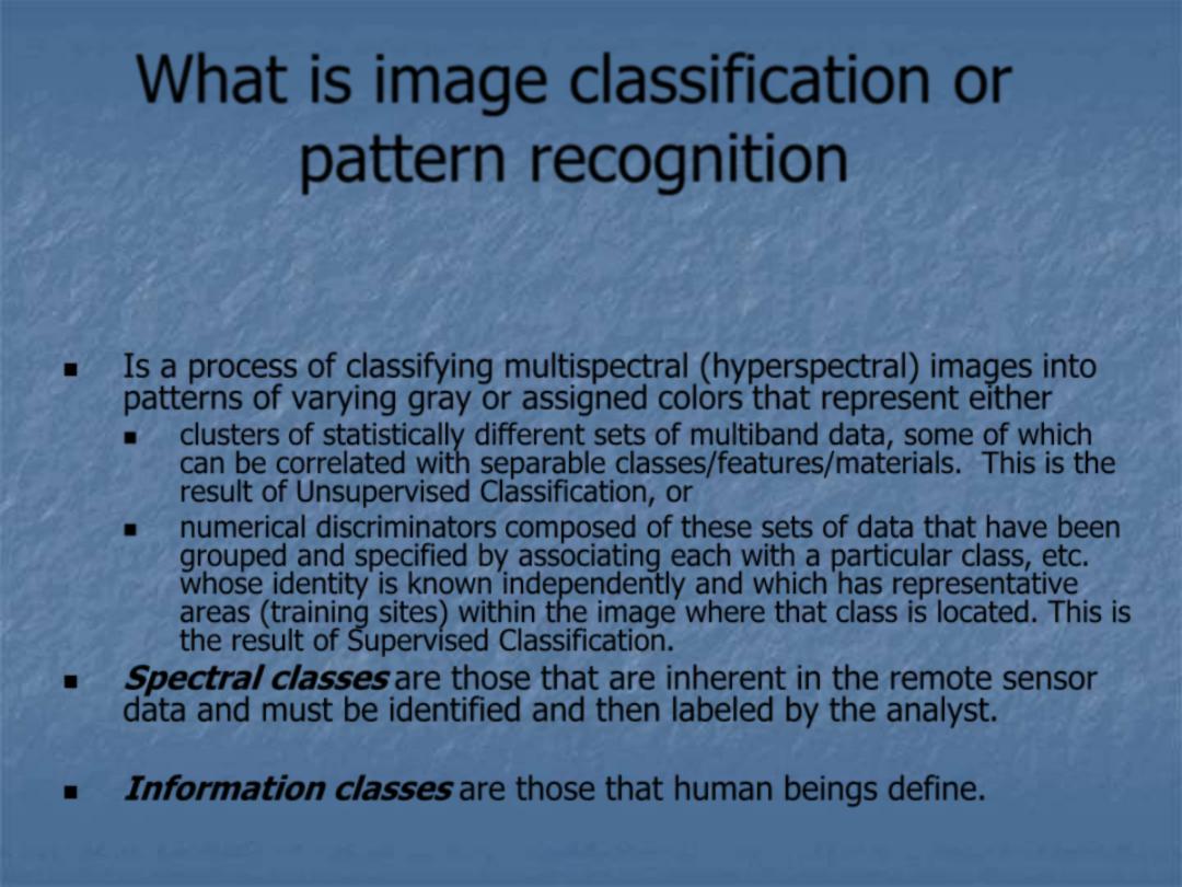
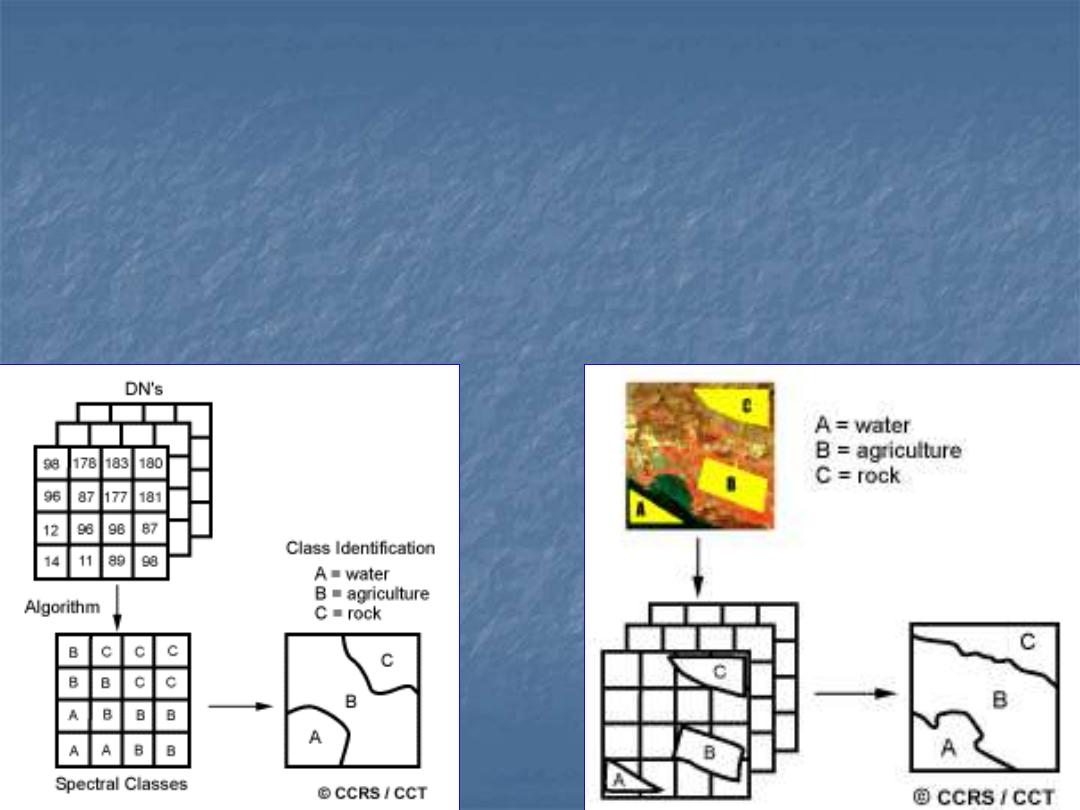
What is image classification or
pattern recognition
Is a process of classifying multispectral (hyperspectral) images into
patterns of varying gray or assigned colors
that represent either
clusters
of statistically different sets of multiband data, some of which
can be correlated with separable classes/features/materials. This is the
result of
Unsupervised Classification
, or
numerical discriminators
composed of these sets of data that have been
grouped and specified by associating each with a particular
class
, etc.
whose identity is known independently and which has representative
areas (training sites) within the image where that class is located. This is
the result of
Supervised Classification
.
Spectral classes
are those that are inherent in the remote sensor
data and must be identified and then labeled by the analyst.
Information classes
are those that human beings define.
supervised classification
. Identify known a priori
through a combination of fieldwork, map
analysis, and personal experience as
training
sites
; the spectral characteristics of these sites are
used to train the classification algorithm for
eventual land-cover mapping of the remainder of
the image. Every pixel both within and outside the
training sites is then evaluated and assigned to the
class of which it has the highest likelihood of
being a member.
unsupervised classification
, The
computer or algorithm automatically
group pixels with similar spectral
characteristics (means, standard
deviations, covariance matrices,
correlation matrices, etc.) into unique
clusters according to some statistically
determined criteria. The analyst then
re-labels and combines the spectral
clusters into information classes.
Unsupervised classification
Uses
statistical techniques
to group n-dimensional data into their natural
spectral clusters, and uses the
iterative procedures
label certain clusters as specific information classes
K-mean and ISODATA
For the first iteration arbitrary
starting values
(i.e., the cluster properties)
have to be selected. These
initial values
can influence the outcome of the
classification.
In general, both methods assign first arbitrary initial cluster values. The
second step classifies each pixel to the closest cluster. In the third step the
new cluster mean vectors are calculated based on all the pixels in one
cluster. The second and third steps are repeated until the "change" between
the iteration is small. The "change" can be defined in several different ways,
either by measuring the distances of the mean cluster vector have changed
from one iteration to another or by the percentage of pixels that have
changed between iterations.
The
ISODATA algorithm has some further refinements
by splitting and
merging of clusters. Clusters are merged if either the number of members
(pixel) in a cluster is less than a certain threshold or if the centers of two
clusters are closer than a certain threshold. Clusters are split into two
different clusters if the cluster standard deviation exceeds a predefined value
and the number of members (pixels) is twice the threshold for the minimum
number of members.
Supervised classification:
training sites selection
Based on known a priori through a combination of fieldwork,
map analysis, and personal experience
on-screen selection
of polygonal training data (ROI),
and/or
on-screen seeding
of training data (ENVI does not have
this, Erdas Imagine does).
The
seed program
begins at a single
x, y
location and evaluates
neighboring pixel values in all bands of interest. Using criteria
specified by the analyst, the seed algorithm expands outward like
an amoeba as long as it finds pixels with spectral characteristics
similar to the original seed pixel. This is a very effective way of
collecting homogeneous training information.
From
spectral library
of field measurements
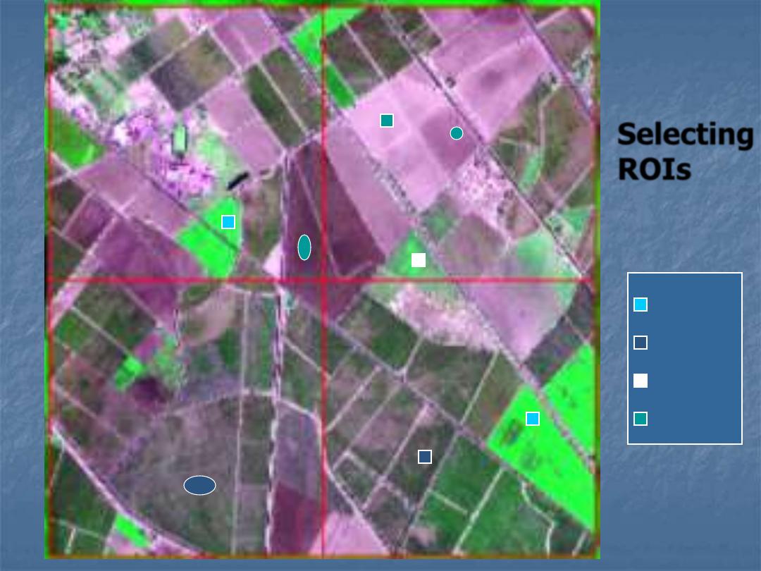
Selecting
ROIs
Alfalfa
Cotton
Grass
Fallow
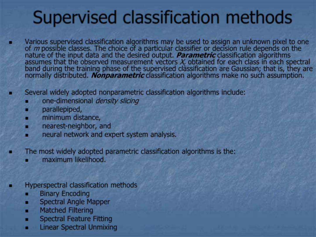
Supervised classification methods
Various supervised classification algorithms may be used to assign an unknown pixel to one
of
m
possible classes. The choice of a particular classifier or decision rule depends on the
nature of the input data and the desired output.
Parametric
classification algorithms
assumes that the observed measurement vectors
X
c
obtained for each class in each spectral
band during the training phase of the supervised classification are
Gaussian
; that is, they are
normally distributed.
Nonparametric
classification algorithms make no such assumption.
Several widely adopted nonparametric classification algorithms include:
one-dimensional
density slicing
parallepiped
,
minimum distance
,
nearest-neighbor
, and
neural network
and
expert system analysis
.
The most widely adopted parametric classification algorithms is the:
maximum likelihood
.
Hyperspectral classification methods
Binary Encoding
Spectral Angle Mapper
Matched Filtering
Spectral Feature Fitting
Linear Spectral Unmixing
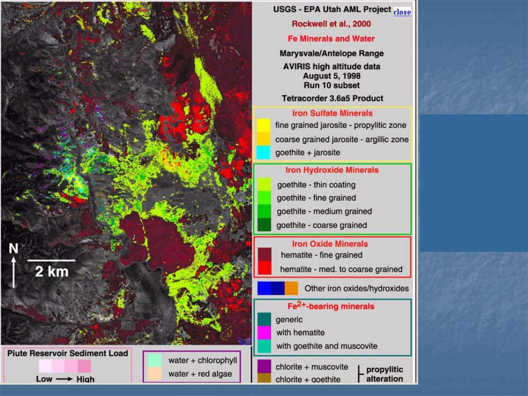
Source: http://popo.jpl.nasa
.gov/html/data.html
Supervised
classification
method:
Spectral Feature
Fitting
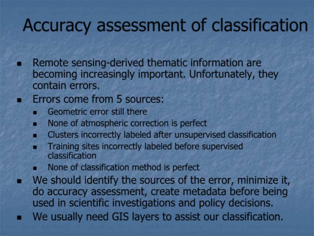
Accuracy assessment of classification
Remote sensing-derived thematic information are
becoming increasingly important. Unfortunately, they
contain errors.
Errors come from 5 sources:
Geometric error still there
None of atmospheric correction is perfect
Clusters incorrectly labeled after unsupervised classification
Training sites incorrectly labeled before supervised
classification
None of classification method is perfect
We should identify the sources of the error, minimize it,
do accuracy assessment, create metadata before being
used in scientific investigations and policy decisions.
We usually need GIS layers to assist our classification.
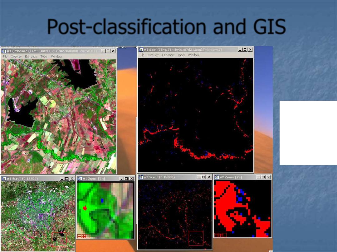
Post-classification and GIS
salt-
and-
pepper
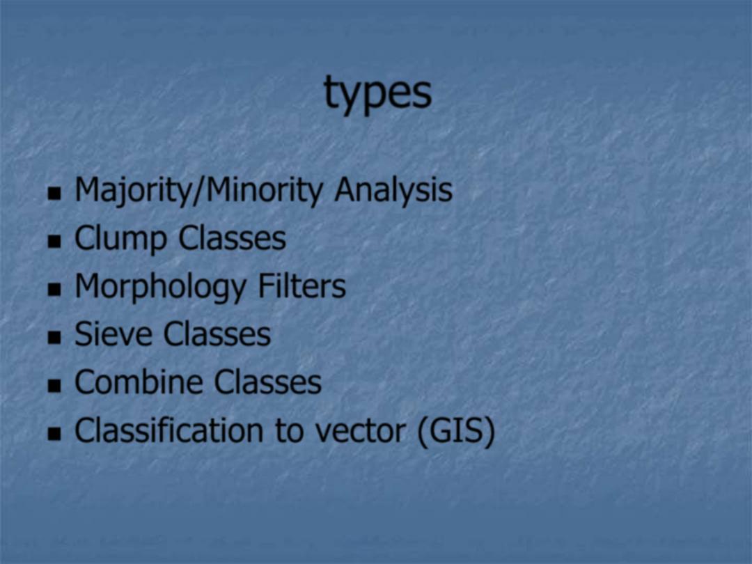
types
Majority/Minority Analysis
Clump Classes
Morphology Filters
Sieve Classes
Combine Classes
Classification to vector (GIS)
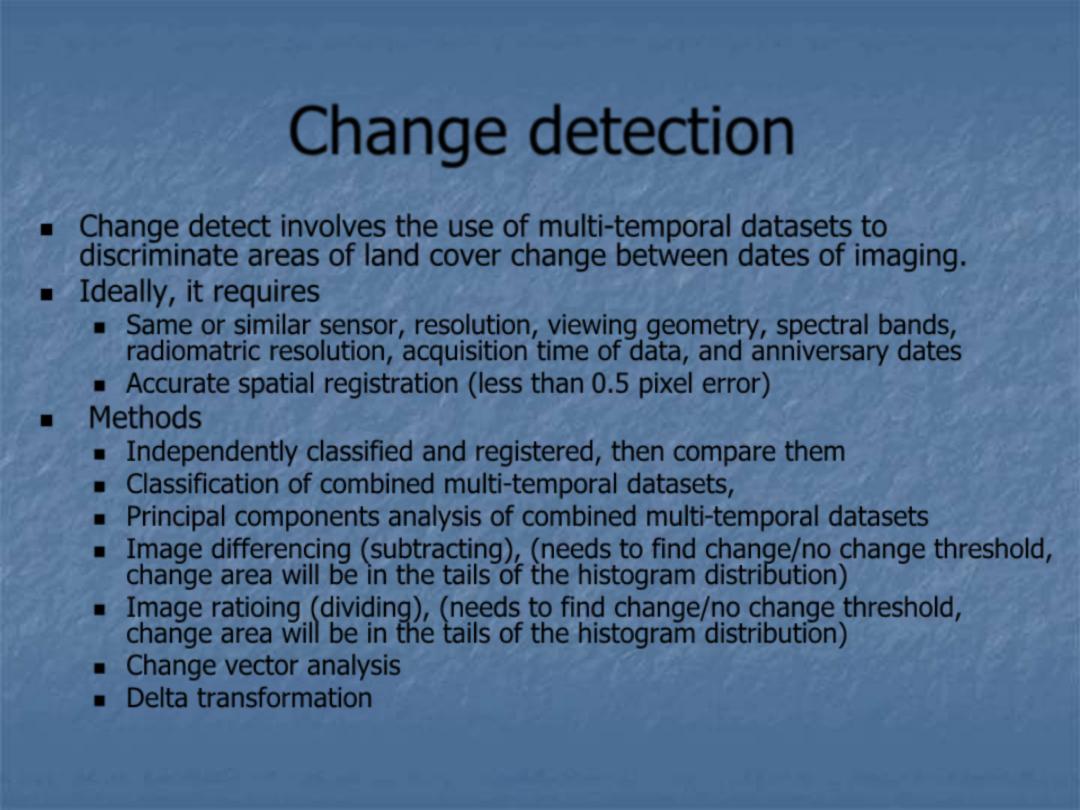
Change detection
Change detect involves the use of multi-temporal datasets to
discriminate areas of land cover change between dates of imaging.
Ideally, it requires
Same or similar sensor, resolution, viewing geometry, spectral bands,
radiomatric resolution, acquisition time of data, and anniversary dates
Accurate spatial registration (less than 0.5 pixel error)
Methods
Independently classified and registered, then compare them
Classification of combined multi-temporal datasets,
Principal components analysis of combined multi-temporal datasets
Image differencing (subtracting), (needs to find change/no change threshold,
change area will be in the tails of the histogram distribution)
Image ratioing (dividing), (needs to find change/no change threshold,
change area will be in the tails of the histogram distribution)
Change vector analysis
Delta transformation
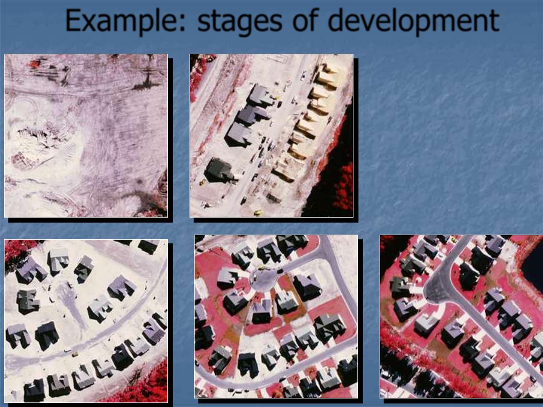
Example: stages of development
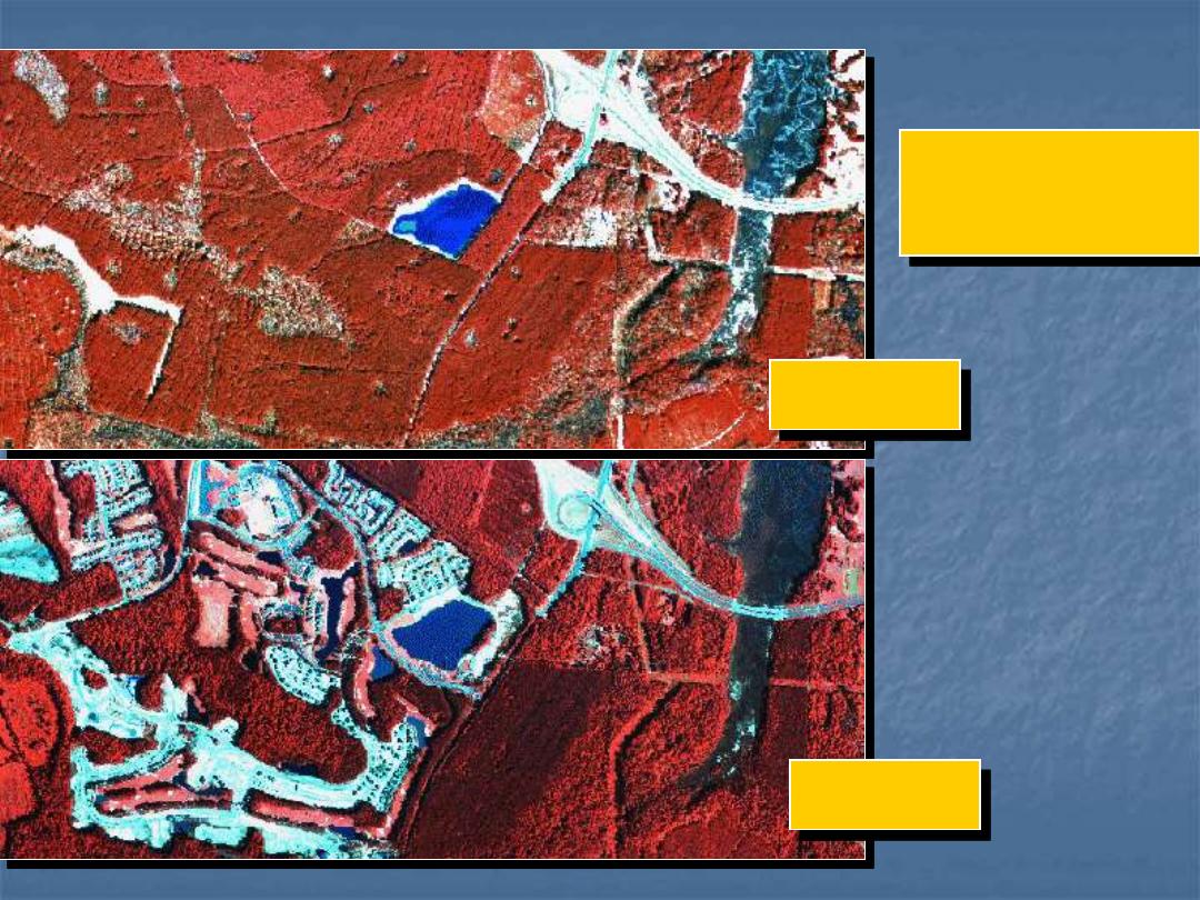
1994
1996
Sun City –
Hilton Head
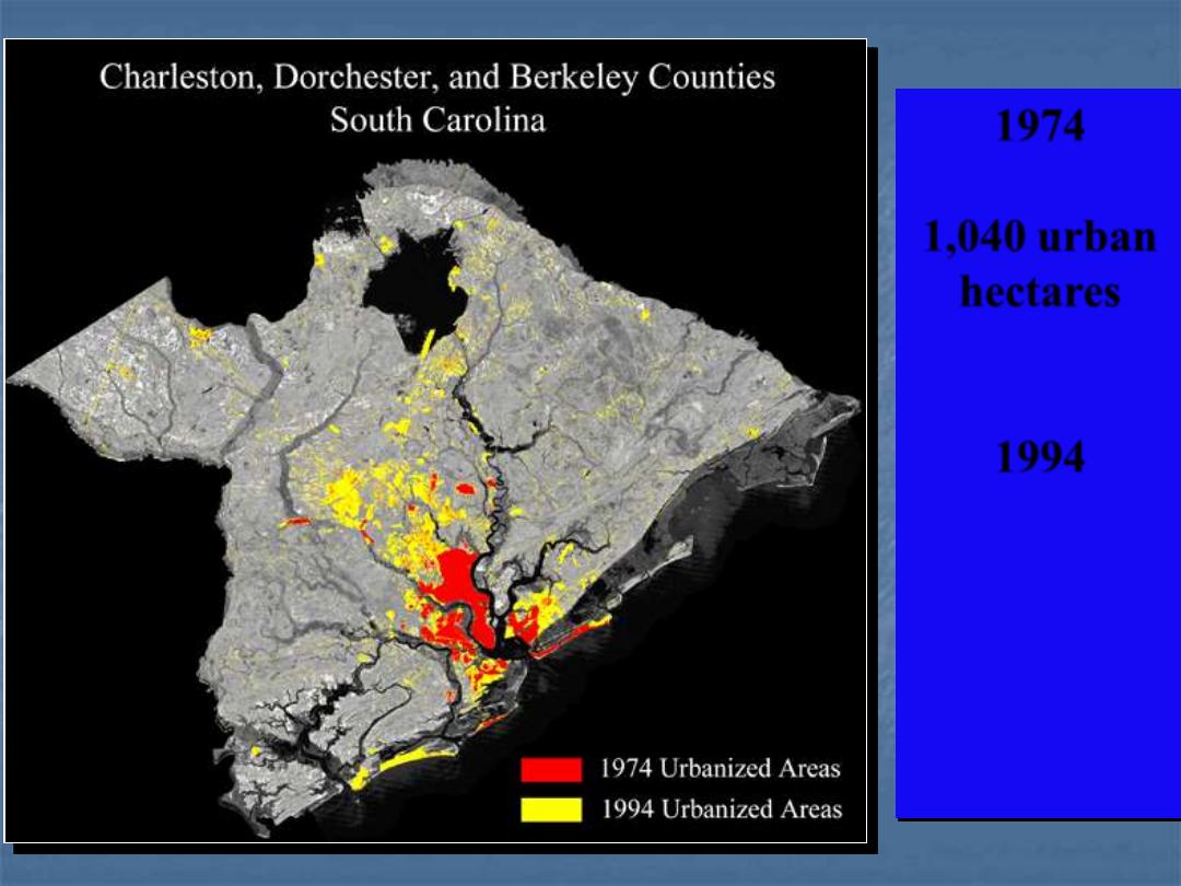
1974
1,040 urban
hectares
1994
3,263 urban
hectares
315%
increase