Statistics

Biostatistics-Lecture 13rd stage-College of MedicineOctober 17th , 2021

By Dr. Muslim N. Saeed
Family & Community Medicine dept.

Learning objective: - To understand the basic statistical principles commonly used in Public Health.- Defining statistics and biostatistics.- Understand the meaning of variables and knowing their types.- Understand the methods of representing data.-

Introduction

"The importance of medical statistics“
Statistics is a fundamental tool for investigation in all biological and medical science. As such, any serious investigator in these fields must have a grasp of the basic principles.
With modern computer facilities there is little need for familiarity with the technical details of statistical calculations. However, a health care professional should understand when such calculations are valid, when they are not and how they should be interpreted.

Statistic is the field of study which can be classified into;

1) Descriptive: Concern with collection, classification, organization and summarization (reduction) of the data.
((They are merely descriptive & used to describe the basic features of the data in a study. They provide simple summaries about the measures make no attempt to draw conclusion)). They can be:
a- Tabular ((tables)).
b- Diagrammatic ((Figures)).
c- Numerical ((Numbers)).
2) Inferential: Concern with drawing conclusions from the data that extend beyond the immediate data alone. The conclusion drawn will influence sub- sequent decision.

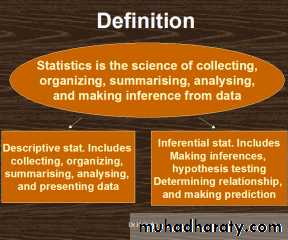
Biostatistics: The statistics that concern with biological& medical aspects.

Uses of Biostatistics:
1) Measure & analyze the health status and health problems in the community.
2) Compare the health status of the community with others.
3) Planning for the health services.
4) Evaluation of the health services & estimation the future needs.
5) For research purposes. "Statistics is vital & central to most medical research".
6) Evaluation of published papers.

 The information about which we are concerned are called data (raw

material of statistics) and these data are a available in form of numbers (values). Two kinds of number are used in statistics;
1) Numbers (values) that result from the process of
counting "Frequencies" e.g. No. of patient admitted
to the hospital per day, No. of teeth……etc.
2) Number (values) that result from measurement e.g.
B.P, Weight, and Height ……etc.
* Sources of data: 1- Experiment. 2- Survey.
3- Routinely kept records.
4) External sources e.g. published reports, Internet.


Quantities; can be classified into:
1) Constants, quantities which are not vary e.g. 3.14 =
this type not need statistical analysis.
2) Variables, quantities which vary (take different values in different person, place, &/or time e.g. WT, HT,
BP..etc; this type need statistical analysis.( Statistics
deals with variables )
 Random variable;
Is the variable that arises as a result of chance factors, so
can't be exactly predicted in advance. e.g. HT, WT,
when a child born, we can't predict exactly his/her HT or
WT at maturity.

Variables are subdivided into;

1) Quantitative (Numerical); can be measured by the usual sense e.g. age, WT, HT….etc. This can be either:
a) Discrete, taking some value in discontinues set of
value (characterized by a gap or interruption, have no
fraction) e.g. No. of teeth, No. of admissions, Number
of children, Number of attacks of asthma per
week….etc..
b) Continuous, taking some value in an infinity divisible
range of value (doesn’t possess a gap or interruption,
have a fraction, we can find another value somewhere
in between) e.g. WT, HT, Serum cholesterol, Blood
sugar….etc.


2) Qualitative (Categorical); can't be measured by the usual sense but must describe in category. This can be either:
a) Nominal, defined by un ordered categories. E.g., color of the eye, blood group, sex, marital state….etc.
(Nominal variable with only two probabilities is called
"dichotomous variable" e.g., life or death, sick or
not ….etc.
b) Ordinal, defined by ordered categories. E.g.,
educational state categorized into primary, secondary
and higher education, Cancer staging I, II, III……etc.

Notes;

I. It is important to be able to distinguish different types of data from one another as we use different techniques to describe and analyses different types.
II. Numerical variables can be converted to Categorical one by using "cut off points".
For example, blood pressure can be turned into a nominal variable by defining "hypertension" as a diastolic blood pressure greater than 90 mmHg, and "normo-tension" as blood pressure less than or equal to 90 mmHg. Height (continuous) can be converted into "short", average" or "tall" (ordinal).
In general it is easier to summarize categorical variables, and so quantitative variables are often converted to categorical ones for descriptive purposes as in make a clinical decision on serum potassium level, one does not need to know the exact serum potassium level (continuous) but whether it is within the normal range (nominal) also It may be easier to think of the proportion of the population who are hypertensive than the distribution of blood pressure.

Methods of presentation of data

A- Numerical presentation
B- Graphical presentation
C- Mathematical presentation

Ordered array: When we arrange our data in order of magnitude from the smallest value to the largest value ((organization of the data)).
Ex; (9, 2, 5, 7, 3, 1) → In ordered array→ (1, 2, 3, 5, 7,9).



Grouped data: A technique used for systematically arranging a collection of observations to indicate the frequency of occurrence of the different values of these observations ((summarization of the data)).






















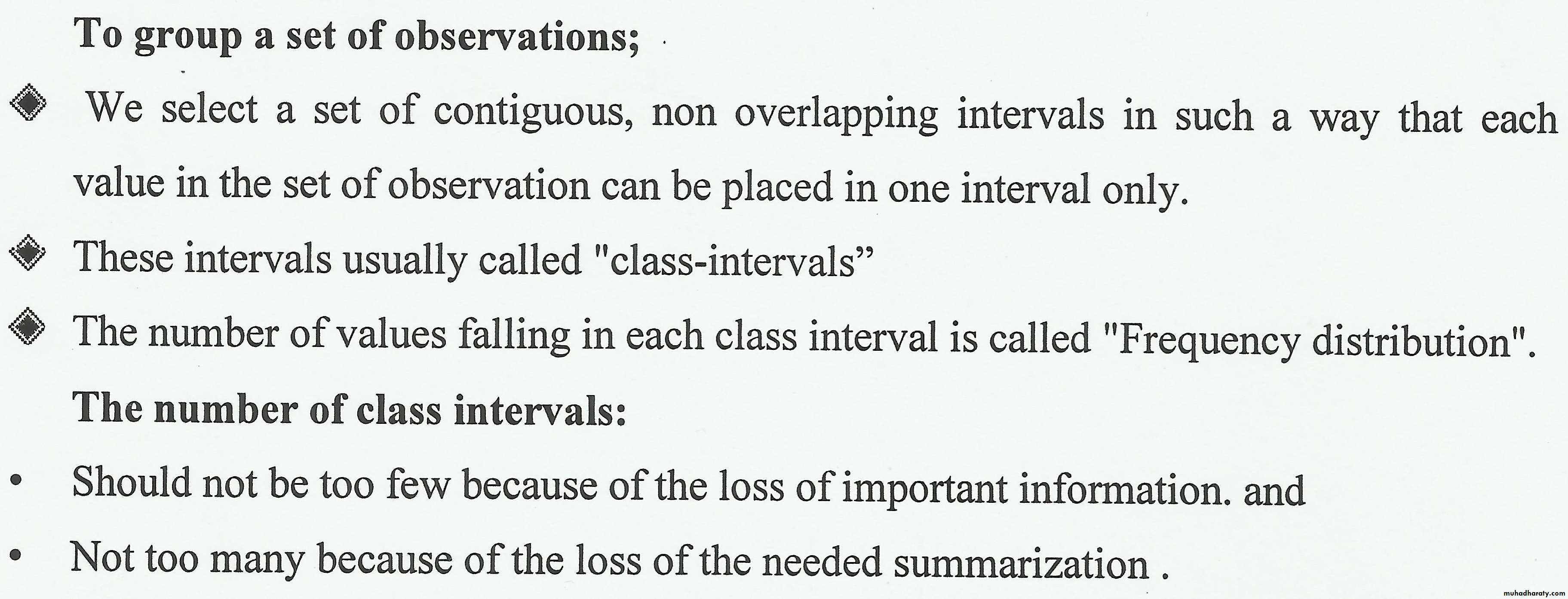
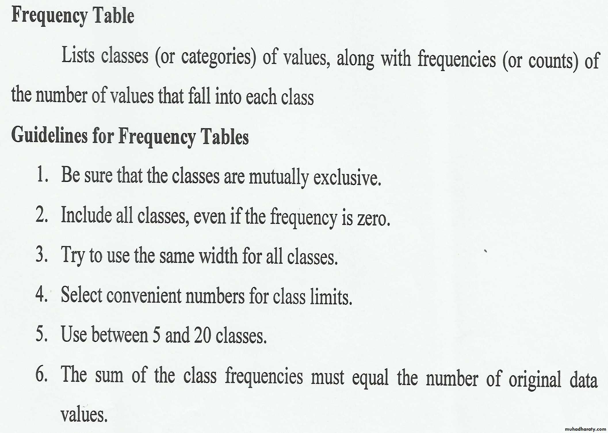
So, to group a set of observations, we select a set of contiguous, non overlapping intervals in such away that each value in the set of observation can be placed in one
interval only, these intervals usually called "class intervals".
The no. of values falling in each class interval
is called "Frequency distribution".

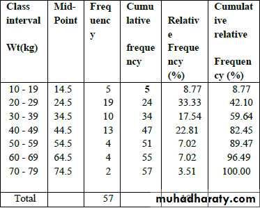
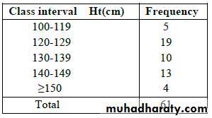
Ex. Frequency distribution of Ht in cm of 61 subjects.

General rules for forming frequency distribution of grouped data.

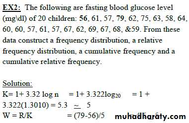
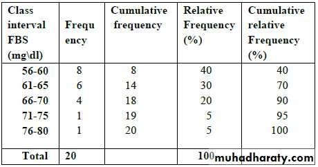
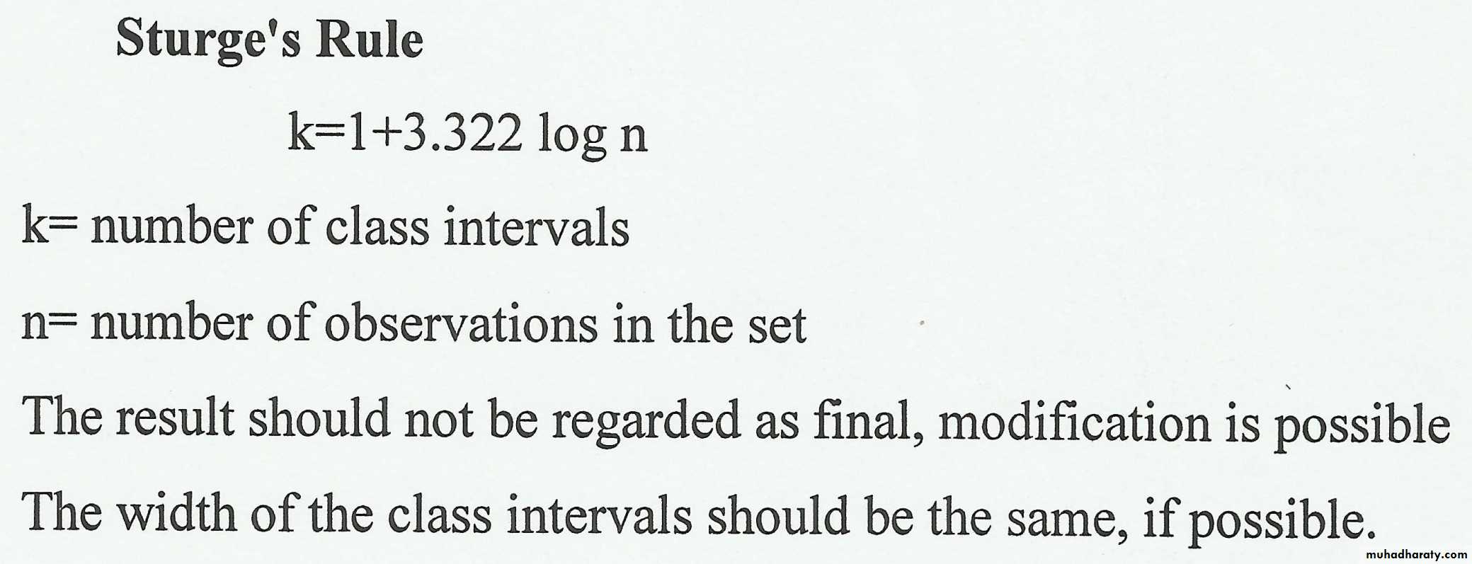
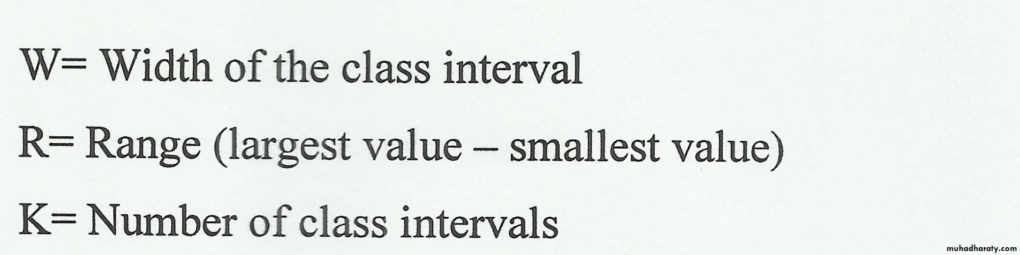
1) Count the number of intervals by using "Sturge's rule":
K = 1+ 3.322 log n (k = no. of class interval, n = sample size).
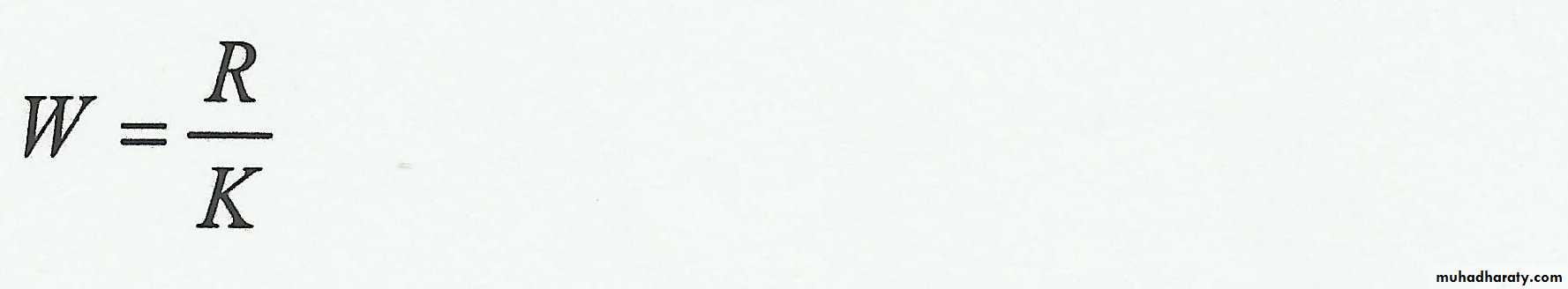
2) Find the width ((W)) of the intervals. The class intervals should be of the same width. W = Range (R) / K ,
R = largest value - smallest one

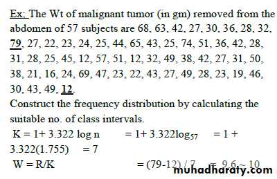
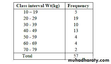
Note. Too few intervals are undesirable because of the

resulting loss of information, and too many intervals will
not meet the objective of summarization.
The Mid-Point of the class interval is obtaining by
computing the mean of the upper & lower limits of the
interval.
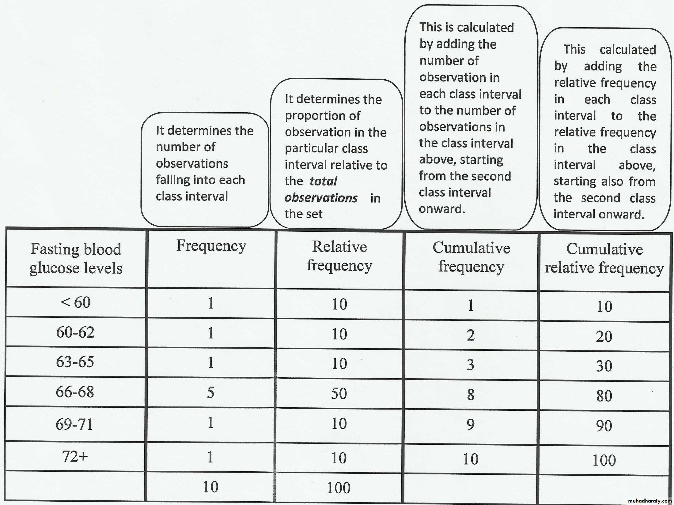
The Cumulative Frequency; is the frequency regarding two or more intervals.
The Relative Frequency; is the proportion of value within each class interval. This is obtained by dividing the class frequency by the total frequency for all classes x100((usually express as percentage)).
The Cumulative Relative Frequency; is the relative
frequency for two or more class intervals ((also usually
express as percentage)).

End