First stage – College of Medicine – University of Mosul
Computer-Lecture 8 / 2015-2016
maha al ani
1
5. Formatting Cells
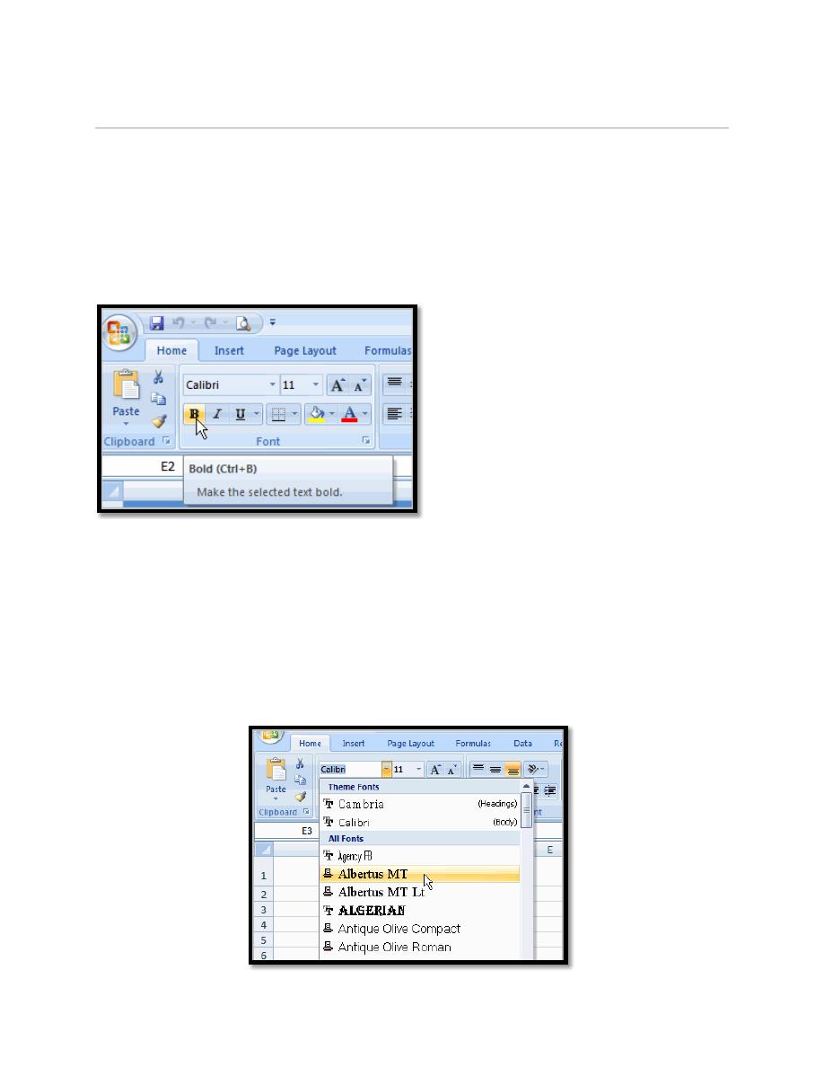
5.1. To Format Text as Bold, Italic and Underlined:
a. Left-click a cell to select it or drag your cursor over the text in the
formula bar to select it.
b. Click the Bold or Italic command.
c. Select the Single Underline or Double Underline option.
5.2. To Change the Font Style
a. Select the cell or cells you want to format.
b. Left-click the drop-down arrow next to the Font Style box on the Home
tab.
c. Select a font style from the list.
First stage – College of Medicine – University of Mosul
Computer-Lecture 8 / 2015-2016
maha al ani
2
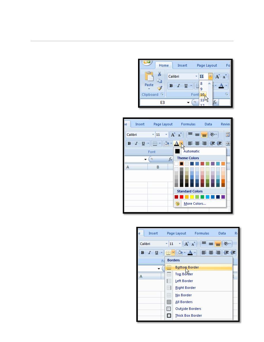
5.3. To Change the Font Size:
a. Select the cell or cells you want to
format.
b. Left-click the drop-down arrow next to
the Font Size box on the Home tab.
c. Select a font size from the list.
5.4. To Change the Text Color:
a. Select the cell or cells you want
to format.
b. Left-click the drop-down arrow
next to the Text Color
command. A color palette will
appear.
c. Select a color from the palette.
5.5. To Add a Border:
a. Select the cell or cells you want to
format.
b. Click the drop-down arrow next to the
Borders command on the Home tab. A
menu will appear with border options.
c. Left-click an option from the list to
select it.
First stage – College of Medicine – University of Mosul
Computer-Lecture 8 / 2015-2016
maha al ani
3
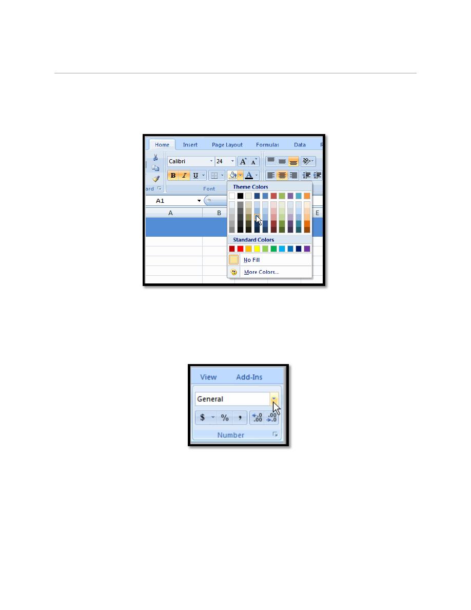
5.6. To add a Fill Color:
a. Select the cell or cells you want to format.
b. Click the Fill command. A color palette will appear.
c. Select a color.
5.7. To Format Numbers and Dates:
a. Select the cell or cells you want to format.
b. Left-click the drop-down arrow next to the Number Format box.
c. Select one of the options for formatting numbers.
6. Working with Cells
6.1. To Copy and Paste Cell Contents:
a. Select the cell or cells you wish to copy.
b. Click the Copy command in the Clipboard group on the Home tab. The border
of the selected cells will change appearance.
c. Select the cell or cells where you want to paste the information.
First stage – College of Medicine – University of Mosul
Computer-Lecture 8 / 2015-2016
maha al ani
4
d. Click the Paste command. The copied information will now appear in the new
cells.
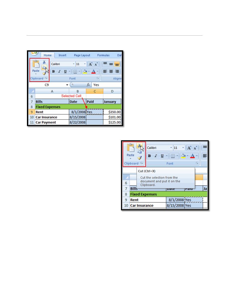
6.2. To Cut and Paste Cell Contents:
a. Select the cell or cells you wish to cut.
b. Click the Cut command in the
Clipboard group on the Home tab. The
border of the selected cells will change
appearance.
c. Select the cell or cells where you want
to paste the information.
d. Click the Paste command. The cut
information will be removed from the
original cells and now appear in the new
cells.
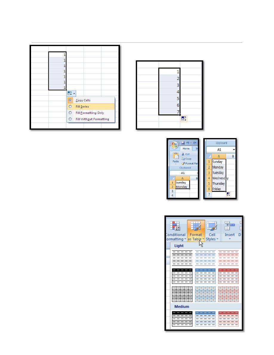
6.3. To Use the Fill Handle to Fill Cells:
a. Position your cursor over the fill handle until the large white cross becomes a
thin, black cross.
b. Left-click your mouse and drag it until all the cells you want to fill are
highlighted.
c. Click the arrow appears after dragging the mouse, the menu appears contains fill
series command.
d. Release the mouse button and all the selected cells are filled.
First stage – College of Medicine – University of Mosul
Computer-Lecture 8 / 2015-2016
maha al ani
5
AutoFill
Enter the months of the year, the days of the week,
multiples of 2 or 3, or other data in a series. You
type one or more entries, and then extend the
series.
7.
Formatting Tables
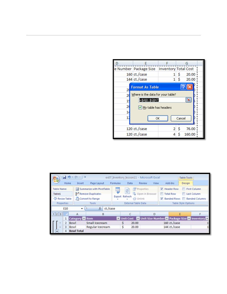
7.1. To format a table:
a.
Select any cell that contains information.
b.
Click the Format as Table command in the
Styles group on the Home tab. A list of predefined
tables will appear.
First stage – College of Medicine – University of Mosul
Computer-Lecture 8 / 2015-2016
maha al ani
6
c.
Left-click a table style to select it.
d.
A dialog box will appear. Excel has automatically selected the cells for your
table. The cells will appear selected in the spreadsheet and the range will appear in
the dialog box.
e.
Change the range listed in the field,
if necessary.
f.
Verify the box is selected to indicate
your table has headings, if it does.
g.
Deselect this box if your table does
not have column headings.
h.
Click OK. The table will appear
formatted in the style you chose.
7.2. To Modify a Table:
Select any cell in the table. The Table Tools Design tab will become active. From
here you can modify the table in many ways.
You can:
a. Select a different table in the Table Styles Options group. Click the More drop-
down arrow to see more table styles.
b. Delete or add a Header Row in the Table Styles Options group.
First stage – College of Medicine – University of Mosul
Computer-Lecture 8 / 2015-2016
maha al ani
7
c. Insert a Total Row in the Table Styles Options group.
d. Remove or add banded rows or columns.
e. Make the first and last columns bold.
f. Name your table in the Properties group.
g. Change the cells that make up the table by clicking Resize Table.
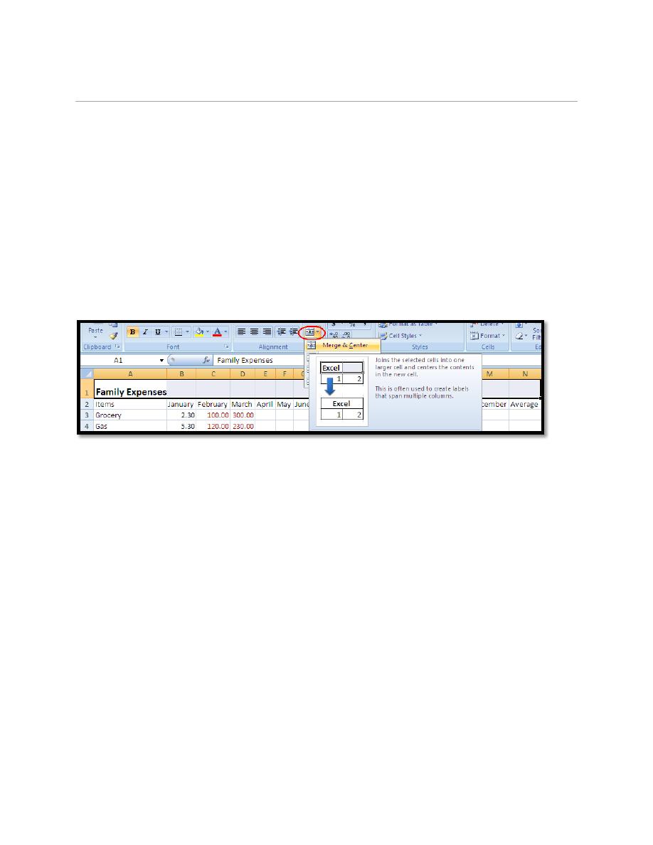
You may want to add a title for an Excel table:
Insert a row above the column heading row.
Type the title in the first cell of the title row.
Highlight the cells you would like to display the table title.
Click on Merge and Center icon.
8. Sorting and Filtering Cells
Sorting lists is a common spreadsheet task that allows you to easily reorder your
data. The most common type of sorting is alphabetical ordering, which you can do
in ascending or descending order.
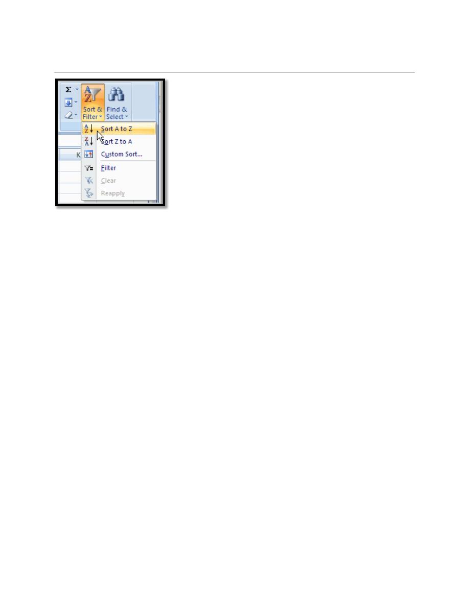
8.1. To Sort in Alphabetical Order:
a. Select a cell in the column you want to sort (In this example, we choose a cell in
column A).
b. Click the Sort & Filter command in the Editing group on the Home tab.
c. Select Sort A to Z. Now the information in the Category column is organized in
alphabetical order.
First stage – College of Medicine – University of Mosul
Computer-Lecture 8 / 2015-2016
maha al ani
8
You can Sort in reverse alphabetical order by choosing Sort Z to A in the list.
8.2. To Sort from Smallest to Largest:
a. Select a cell in the column you want to sort (a column with numbers).
b. Click the Sort & Filter command in the Editing group on the Home tab.
c. Select From Smallest to Largest. Now the information is organized from the
smallest to largest amount.
You can sort in reverse numerical order by choosing From Largest to Smallest in
the list.