
1
1
Q1. A study conducted in Uganda to assess the role of lack of male circumcision on the
risk of HIV acquisition and transmission. 4608 non circumcised males and 908
circumcised males included and followed for 10 years. All were seronegative to HIV at
the start. At the end of the follow up period, 154 among from the first group and 18
among the second group were seropositive to HIV.
• Construct the suitable table
• Calculate the measure of association
• Calculate the measures of Public Health Impact
• Interpret your results
HIV +
HIV −
Total
Cir cum−
154
4,454
4,608
Cir cum+
18
890
908
Total
172
5,344
5,516
§
HIV seroconversion in uncircumcised men
154 seroconversions
4608 men at start of follow-up period
Risk = 154 / 4608 = 0.0334 = 3.34%
§
HIV seroconversion in circumcised men
18 seroconversions
908 men at start of follow-up period
Risk = 18 / 908 = 0.0198 = 1.98%
RR = 3.34 / 1.98 = 1.7
Interpretation: lack of circumcision associated with 1.7 times excess risk of HIV as
compared to circumcised males
AR = Incidence
exposed
-Incidence
non-expose d
=3.34% - 1.98%= 1.36%
Interpretation: There is around 1.4 HIV cases among each 100 uncircumcised males
attributed to lack of circumcision (14 /1000)
AR% = [AR / Incidence
exposed
] x 100
=[1.36%
/
3.34%] X 100
= 40.7%
Interpretation: Around 41% of HIV cases among uncircumcised males are attributed to
lack of circumcision
PAR% = [(I
population
-
I
unexposed
)/ I
population
] x100
I
population
= 162/5516 X100%= 2.94%
PAR% = [(2.94%
-
1.98%) / 2.94%] x100
= 32.7%
Interpretation: if circumcision is applied to all males, around 33% of HIV cases will be
prevented

2
2
Q2) Comparison of impacts of Beta-blockers, ACE inhibitors, spironolactone on all-
cause mortality within one year of hospitalization for congestive heart failure, using
the risk estimates in the Australian (Hunter area) population.
Bet a-
block ers
ACE
inhibitors
Spironolacton
e
Incidence of death am ong unt reat ed
(exposed)
0.29
0.29
0.29
Incidence of death am ong treated
(unexposed)
0.1914
0.2436
0.203
Calculate the attributable risk (AR) and Attributable risk percent (AR%).
Which of the three tested interventions (treatments) conveys the highest protection?
If 100 subjects with congestive heart failure is treated with beta-blockers how many
potential deaths would be prevented?
Beta-blockers ACE inhibitors Spironolactone
Rat e
per 100
person
Rate
per 100
person
Rat e
per 100
person
Incidence of death am ong unt reat ed
(I
exposed
)
0.29
29
0.29
29
0.29
29
Incidence of death am ong treated
(I
unexposed
)
0.1914
19.1
0.2436 24.4
0.203
20.3
Absolute risk reduct ion (att ributable
risk)
0.0986 9.9
0.0464 4.6
0.087
8.7
Att ributable risk percent
34.0
16.0
30.0
Relat ive risk
1.52
1.19
1.43
AR=Ie-Iu
AR%=(AR/Ie)x100
RR=Ie/Iu
By comparing the AR%, one concludes that Beta-blockers provides the highest
protection, followed by spironolactone and the least protective is ACE inhibitors.
Treatment with Beta-blockers would prevent 34% of potential deaths among patients
with congestive heart failure, while ACE inhibitors prevent only 16% of potential
deaths.
If 100 subjects with congestive heart failure is treated with beta-blockers it is
expected to prevent 9.9 deaths.

3
3
Q3) Data collected during the course of a cohort study which compared mortality
amongst cigarette smokers with non-smokers in young adults during a 7-year period.
Smo k ing hab it
Tot al N
Died w ithin 7
year s
Cigarett e smokers
25769
133
Non-smokers
5439
3
Incide nce of deat h in young adult population (during 7 ye ars) = 230 / 100,000 person
What is the risk of dying (during 7 years) for smokers and non-smokers?
Do you agree that smoking is bad for health?
Can you express the magnitude of association between smoking and death?
How many deaths can be prevented among 1000 smokers during the coming 7 years if
they quit smoking now?
How important is smoking as a potential cause of death among young adults?
If smoking was eliminated at the population level, what is the expected benefit, would
you advice a smoking cessation campaign?
Absolut e risk (incidence of de ath) in cigare tt e smokers=516 per 100,000
Absolut e risk (incidence of de ath) in non-smokers=55 per 100,000
Incide nce of deat h in young adult population (during 7 ye ars) = 230 / 100,000 person
Relative risk in cigare tt e smokers =516/ 55=9.4 (the 7 ye ars risk of dying among
smokers is 9.4 t imes higher than that among non-smoke rs). Smoking is indeed bad
for health.
At tribut able risk of cigaret te smoking =516-55=460 per 100,000 (or 4.6 per 1000, for
e ach 1000 smokers who quit smoking we expe ct t o prevent 4.6 pot ent ial deaths
during 7 ye ars).
At tribut able risk % (AR%) = (460/ 516)x100=89%. The proport ion of deat hs in
smokers t hat would be eliminat ed by ce ssat ion of smoking is 89%. Smoking is t he
most important cause of deat h in young adults, sharing responsibility for 89% of
deaths in this group.
Populat ion Att ributable risk % (PAR%) = ((I
population
-I
une xpose d
)/ I
population
)x100
= ((230-55)/ 230)x100=70.1%.
If smoking was eliminat ed from the populat ion of young adult s one can prevent
70.1% of possible deat hs in t his population sect or. A smoking cessation campaign is
a reasonable and advisable approach based on PAR%.

4
4
Q4) A case control study was conducted to assess the effect of two exercise initiatives
on body mass index (BMI). The results from the study are given below
Exercise program
Num ber of
participants
BMI before
exercise
program
BMI aft er
exercise
program
P value for
t he change
in BMI after
exercise
Giving free vouchers for the
gym
17
27+ / -8
23+ / -10
0.09
Having a free personal trainer
20
30+ / -12
24+ / -15
0.02
Note: Mean+/-SD
What measure of effect size is needed to evaluate the impact of exercise on BMI?
Which exercise program is more effective in management of obesity?
The mean difference (since this is a paired design or before-after design, while
difference between two means is used in the independent samples design, such as the
difference between the two types of exercise programs) is the measure of effect size.
The mean difference in BMI for the first type of exercise program (Giving free
vouchers for the gym) = 23-27= -4 kg/m
2
. This program is associated with a mean
reduction in BMI of 4 kg/m2. The observed difference was however not significant
statistically (P > 0.05).
The mean difference in BMI for the second type of exercise program (Having a
free personal trainer) = 24-30= -6 kg/m2. This program is associated with a statistically
significant mean reduction in BMI of 6 kg/m2.
Having a free personal trainer is more effective in lowering BMI than "Giving
free vouchers for the gym".
5
5
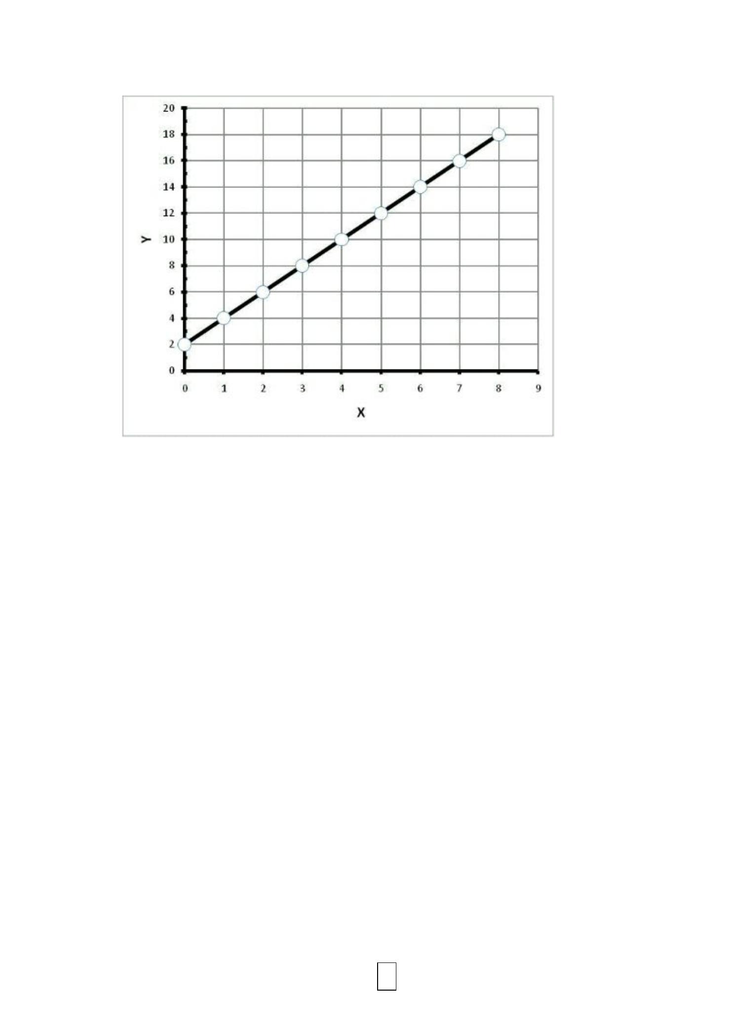
Q5) The above diagram shows the relation between X and Y, which are two
quantitative normally distributed variables measured on an interval/ratio
scale level.
1. Write the linear regression equation model for Y over X.
2. The Pearson Linear Correlation Coefficient between X and Y = _____.
3. Interpret the value of r?
4. If the value of X=12, you can expect the value of Y to be ________.
5. The regression coefficient measured in another occasion (for the same X
and Y variables and the same units of measurements) was 1.5. Is the effect
of X over Y stronger or weaker than the effect size in the current example.

6
6
1. Y=2+2X. (for each one unit increase in variable X, there is an associated increase of
variable Y by 2 units).
2. r=1
3. Very strong (perfect) positive (direct) linear correlation between X and Y.
4. Y=26
5. The effect is weaker, since the linear regression coefficient in the second study,
which is 1.5 is smaller than the present study, which is 2.
7
7
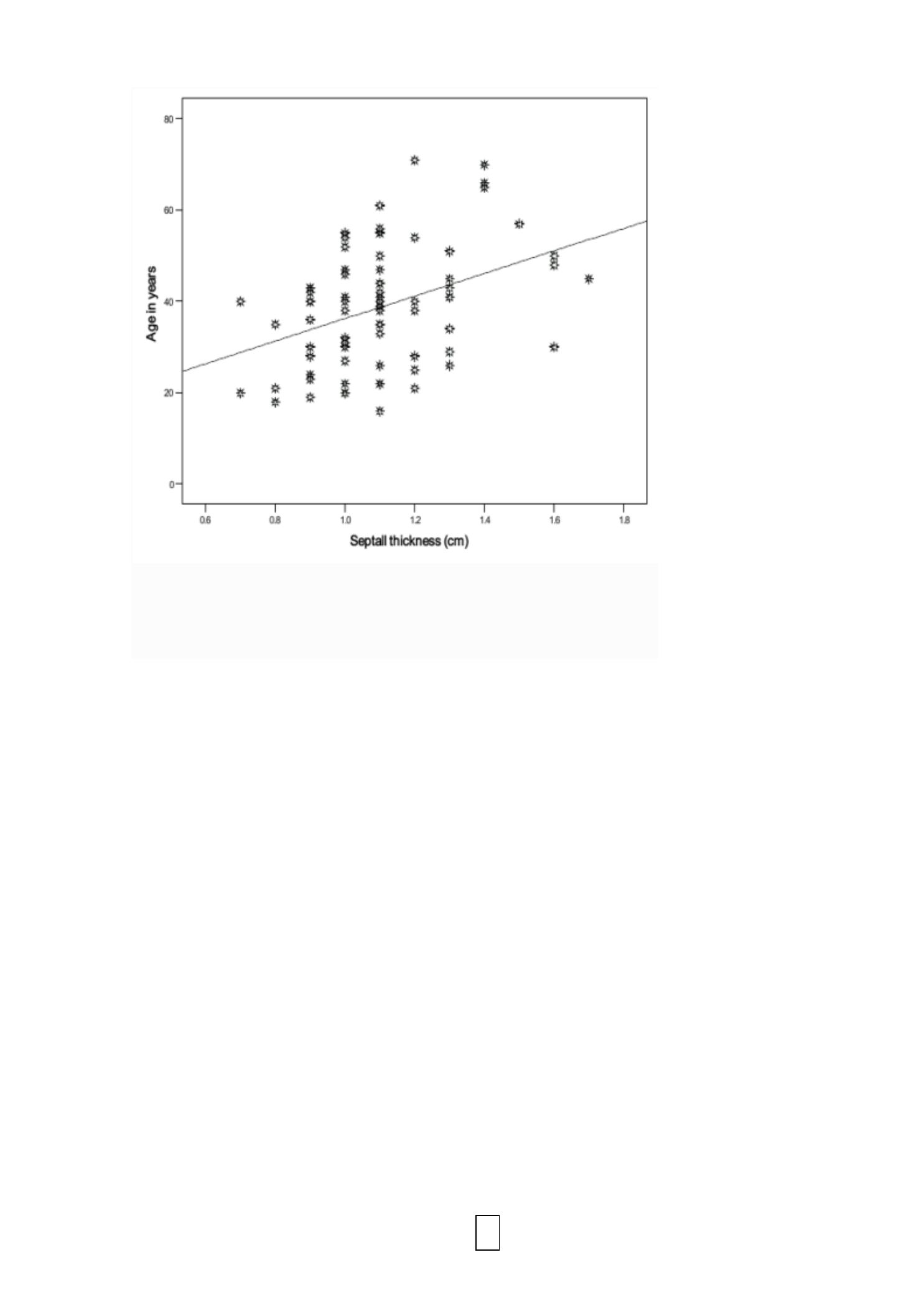
Q6) What do you call this figure? What is the level of measurement for the two
variables shown in the figure? Do you think that the effect of age on cardiac septal
wall thickness is weak, moderate or strong? Septal wall thickness is expected to
decrease with age, is this correct?
This is a scatter diagram
Interval ratio scale
Moderate effect
Incorrect, there is a positive (direct) linear correlation between age and septal wall
thickness.